Dynamical entanglement transition in the probabilistic control of chaos
Abstract
We uncover a dynamical entanglement transition in a monitored quantum system that is heralded by a local order parameter. Classically, chaotic systems can be stochastically controlled onto unstable periodic orbits and exhibit controlled and uncontrolled phases as a function of the rate at which the control is applied. We show that such control transitions persist in open quantum systems where control is implemented with local measurements and unitary feedback. Starting from a simple classical model with a known control transition, we define a quantum model that exhibits a diffusive transition between a chaotic volume-law entangled phase and a disentangled controlled phase. Unlike other entanglement transitions in monitored quantum circuits, this transition can also be probed by correlation functions without resolving individual quantum trajectories.
The dynamics of quantum many-body systems host a range of phenomena usually out of reach to the classical world. Of particular relevance is the ability to locally measure and control systems to enable quantum technological applications such as efficient state preparation [1, 2, 3, 4], quantum error correction [5, 6], and non-destructive measurements [7, 8]. Allowing such nonunitary “hybrid” dynamics in the evolution of many-body states enriches the problem beyond simple, unitary evolution alone. This has recently led to the discovery of phases and phase transitions in the entanglement structure due to the competition between entangling unitary dynamics and projective local measurements [9, 10, 11, 12].
The measurement-induced phase transition (MIPT) in its original formulation entails a fundamental change in the scaling of entanglement from volume- to area-law that is connected to percolation [11, 13, 14], but it has grown past that paradigm and has been studied in numerous contexts [15, 16, 17, 18, 19, 20, 21, 22, 23, 24, 25, 26, 27, 28, 29, 30, 31, 32, 14, 33, 34, 35, 36, 37, 38, 39, 40, 41, 42, 43, 44, 45, 46, 47, 48, 49, 50, 51, 52, 53, 54, 55, 56]. While several incarnations of the transition have been demonstrated, this entanglement transition can only be witnessed by quantities that are non-linear in the density matrix; correlation functions averaged over measurement outcomes are unaffected by the local measurements in the long-time limit. This makes observing the MIPT in experiment a significant challenge requiring either postselection or decoding.
If, on the other hand, we augment each local measurement with control [57, 58] (i.e., unitary feedback conditioned on the measurement outcome), it should be possible to stabilize a dynamical phase transition that is observable in quantities that are linear in the density matrix. In this work, we identify such a control transition in an open quantum many-body system. Unlike previously studied MIPTs, incorporating local feedback into the dynamics leads to a unique control transition visible in both entanglement measures and correlation functions, making it observable using current experimental setups.
The central idea stems from classical dynamical systems, where methods to control chaotic dynamics have been developed. The control protocols can be either deterministic, requiring constant monitoring and perturbation [59], or probabilistic [60, 61]. The latter entails the coupled stochastic action of a chaotic map (with probability ) together with a control map (with probability ). These two coupled maps have the same periodic orbit, unstable for the chaotic map and stable for the control map. Under the stochastic action of the coupled map, the periodic orbit becomes the global attractor at some critical control rate . Prima facie, the control transition in these maps seems to mirror certain aspects of MIPTs, albeit at a purely classical level, with the control map as a classical proxy for quantum measurements. The question then naturally arises of whether we can construct a quantum version of probabilistic control transitions and contrast these with quantum MIPTs.
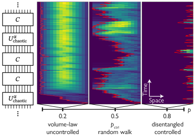
In this paper, starting from a classically chaotic map with a known control transition, we construct a suitable quantum model involving measurements and feedback in which the control transition is enriched by quantum entanglement. The phase transition in the quantum model can be probed by an appropriate local order parameter, and is diffusive with dynamic exponent and correlation length exponent , similar to the classical case. However, the transition is also observed in entanglement and purification measures traditionally used to diagnose MIPTs, which have no analogue in the classical limit. In contrast to the feedback-free MIPTs, the entanglement entropy grows diffusively at the transition before saturating to an area-law value. Many properties of the transition can be understood by tracking the dynamics of an emergent semiclassical domain wall, which undergoes an unbiased random walk at the transition, see Fig. 1.
Model. One of the simplest classical models with a control transition is the Bernoulli map [62]. This map operates on the phase space and is given by
| (1) |
It has a Kolmogorov-Sinai entropy of [62]. In this chaotic map, any rational number such that 2 does not divide undergoes a finite-length periodic orbit. For instance, if , then and ; this is a periodic orbit of length 2. However, since the rational numbers are a set of measure zero in the interval , almost every initial state in the interval undergoes chaotic dynamics. To control this dynamics onto a periodic orbit of our choosing (with points ), we define connected regions such that and , yielding the control map [60]
| (2) |
Note that the points are attractive fixed points of the control map for . We then consider a discrete-time stochastic dynamics in which, at each time step, the chaotic map (1) is applied with probability and the control map is applied with probability . For a critical control rate , there is a phase transition between an uncontrolled phase in which the system never reaches the periodic orbit and a controlled phase in which the system always reaches the orbit. For each value of in Eq. (2), there is a different [61].
To rephrase this model in a manner compatible with quantum mechanics, we map it to a system of qubits as follows. Write the point in base 2 as where . Then, , or in other words, Eq. (1) implements a leftward shift of the bitstring. Then it is natural to define a Hilbert space spanned by computational basis (CB) states . To make the quantum problem more tractable, we truncate the Hilbert space to consist of bitstrings of length . Upon doing this, we immediately encounter a problem: this map appears to be nonunitary (it erases ), and there is an ambiguity as to the value of . The first solution to this problem is simple: let such that the Bernoulli map becomes the translation operator
| (3) |
However, in this formulation, every initial state belongs to a periodic orbit of length at most . In order to have a notion of chaos in the thermodynamic limit , we need the typical orbit length to be exponential in [63, 64, 65]. To accomplish this, we compose the map in Eq. (3) with a scrambling operation on the last few qubits. We consider two options for the scrambling operation: a “classical” and a “quantum” one. The former acts as a permutation on the 8-dimensional space of bitstrings , while the latter is a Haar-random unitary acting on the last two qubits. The chaotic unitary is then defined as
| (4) |
where is the scrambler and or for quantum or classical, respectively. The unitary map is classical in the sense that it maps CB states to CB states—it is a reversible cellular automaton. We choose such that is a chaotic cellular automaton with typical orbit length [see supplemental material (SM)]. In contrast, has no obvious notion of orbits and generates chaotic quantum dynamics in the sense that an initial CB state develops volume-law entanglement in an time owing to the locality of the scrambler (see SM).
We implement the (inherently nonunitary) control map via measurement and feedback. To build it, we choose the period-2 orbit and set in Eq. (2). For this value of , the classical control transition is known to occur at [61]. It is then useful to break up the control map into the multiplication followed by the the addition . The full control operation is
| (5) |
implements the multiplication as follows. projectively measures qubit in the CB and flips it if the outcome is :
| (6) |
where and project the th qubit onto and , respectively, and is the Pauli- operator at site that sets if we measure . Subsequently, completes the multiplication operation. Next, we apply a controlled adder circuit which acts on as
| (7) |
can be built from local unitary operations as described in the SM. Conditioning the addition on the value of determines whether the control map pushes the initial state toward or .
Putting everything together, the quantum model applies with probability and with probability at a given time step. When the chaotic dynamics is generated by , this stochastic dynamics occurs in the space of CB states, and is therefore equivalent to a probabilistic cellular automaton whose properties vary with . The dynamics in this limit is classical, even though the model is phrased quantum mechanically. When is replaced by , the chaotic dynamics becomes entangling, while disentangles the system by pushing it towards the periodic orbit of the underlying classical model. These dynamics can also be formulated as a quantum channel; with additional dephasing, the superoperator that evolves the average density matrix reduces to the Frobenius-Perron evolution operator for classical phase space distributions (see SM).
Classical transition. Our first order of business is to show that the classical control transition survives the above mapping to qubits. To characterize the transition, we first note that the orbit is a two-dimensional subspace spanned by the CB states and . Thus, the control map (2) steers the system’s dynamics onto Néel-ordered antiferromagnetic states. We probe this order using the order parameter
| (8) |
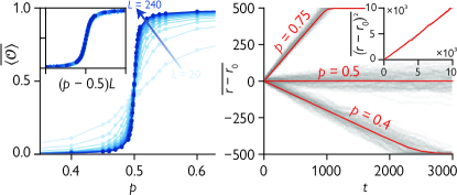
where is the Pauli operator for bit []. The two Néel states maximize , so the controlled phase can be viewed as an ordered phase characterized by in the thermodynamic limit. To probe the transition into the ordered phase in the classical case, we simulate the dynamics of CB states under the stochastic action of and out to time steps for a range of of and . For each and , we calculate at the final time, and average the result over 1000 randomly chosen initial states and circuit instances. We refer to this realization-averaged quantity as . Our results, shown in Fig. 2(left), show that Néel order develops for . Scaling collapse with an ansatz is consistent with a transition point , coinciding with the known result for Eqs. (1) and (2) [61], and with a correlation length critical exponent . Further, the fluctuations of over realizations peak at (not shown), thereby serving as another indicator of the transition.
To further characterize the dynamics at the control phase transition, it is useful to consider the behavior of the “first” (i.e., leftmost) Néel domain wall in the chain, namely the local motif or . The position of the first domain wall (FDW) bounds the distance from a point to the periodic orbit: if the FDW is located on the th bond in the chain, then for . The FDW thus constitutes the boundary between controlled and uncontrolled regions of the qubit chain, see Fig. 1. We simulate the dynamics of the FDW when initialized at and find averaged displacement and mean-squared displacement consistent with a random walk with bias [see Fig. 2(right)]:
| (9) |
Fitting at confirms that , consistent with an unbiased random walk.
Quantum transition. Next, we examine the fate of the control transition when the classical scrambler is replaced by the Haar-random scrambler . Since the hybrid control circuit (2) distributes over superpositions of CB states, a natural hypothesis is that the control transition survives. Then, above some critical , the control circuit drives the system to a disentangled state with as , while below this critical value the system enters a volume-law entangled steady-state with as . Thus, in addition to a control transition, we expect to see an entanglement transition along the lines of those encountered in feedback-free MIPTs, but governed by a distinct universality class.
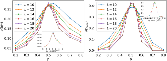
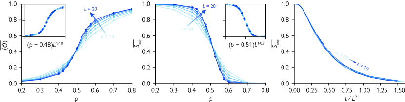
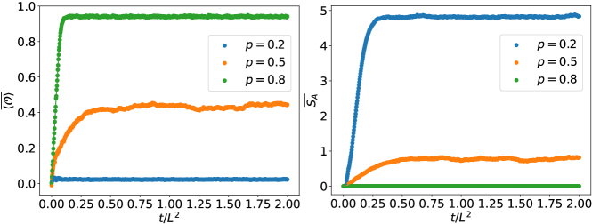
Exact numerical results bear out this simple picture. Fig. 3(left) shows the realization-averaged order parameter as a function of . is measured at time , sufficiently late to ensure that the system reaches a steady state for all values of considered (see SM). Similar to the classical case, there is a clear crossing near . The inset of Fig. 3(left) shows a scaling collapse assuming and , suggesting a control transition near the expected location. In the SM, we show that the fluctuations over realizations of peak at , similarly to the classical transition, and also collapse with .
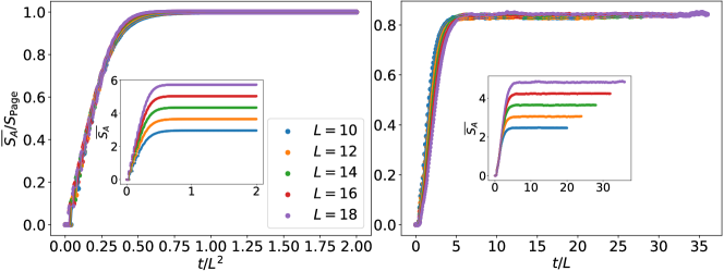
We further investigate the nature of this transition using tools developed for MIPTs. One perspective on MIPTs is that they are purification transitions above which an initially mixed density matrix becomes pure in a finite time [15]. This purification transition can be probed by preparing the system in a maximally entangled state with one ancilla qubit and tracking the ancilla’s entanglement entropy, , as a function of time [66] for varying and . At the purification transition, we expect a crossing of the -vs.- curves for different at times of order . Fig. 3(middle) shows such a crossing near ; the inset shows data collapse assuming and . These data are taken after evolving the system for a time , but the results are insensitive to small variations of this hyperparameter. To characterize the quantum dynamics at the transition, we consider in Fig. 3(right) at . We find that the curves for various nearly collapse upon rescaling with , consistent with the dynamical exponent of the classical transition.
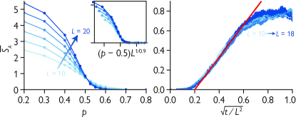
Another perspective on MIPTs is that they constitute a volume-to-area-law transition in the entanglement entropy of a pure state. In Fig. 4, we show that the system’s entanglement entropy is also sensitive to the control transition. We calculate the von-Neumann entanglement entropy of the half-chain, , taking region to be the leftmost sites of the chain. In Fig. 4(left) we show as a function of for different , finding that it increases with for and decreases with for . At the transition, we find that the wavefunction is area-law entangled on average, as indicated by a data collapse (inset) assuming and . In Fig. 4(right), we plot for . The results collapse as a function of (see also Fig. 3) consistent with the classical expectation. In the early-time regime , the realization-averaged entanglement grows diffusively, .
The entanglement properties at the transition can also be understood using the FDW. In the quantum model, the FDW becomes a wavepacket with average position , where is the position of the FDW in the CB state . In the quantum setting, the uncontrolled region to the right of the FDW develops entanglement due to the action of the local scrambler (see Fig. 1). The FDW thus constitutes a front between entangled and disentangled regions, and its dynamics governs that of the half-cut entanglement. At the transition the transport of the FDW is diffusive, so the entanglement dynamics must also be diffusive. Futhermore, since volume-law entanglement can only develop when the FDW “sticks” to the left edge of the chain for at least an time (see SM), which is exponentially unlikely in an unbiased random walk, the average entanglement can be at most area-law at the transition.
Discussion and outlook. In this work, we construct a quantum model that generalizes the stochastic dynamics associated with the probabilistic control of classical chaos. The model exhibits a dynamical entanglement transition reminiscent of MIPTs, but which is also witnessed by a local order parameter. Taken together, our numerical results for the quantum model indicate a diffusive transition at a critical control rate , consistent with both large-system numerics and previous analytical results for the classical version of the transition. The qualitative features of the classical transition are robust to quantum effects, but the entanglement dynamics across the transition has no classical analogue.
A natural question arising from this work is whether other MIPTs can be enriched into control transitions by the addition of feedback (e.g., contingent on what could be learned from the measurement record [55]). If this can be achieved, then the local order parameter for the control transition becomes an indicator for the entanglement transition. An immediate consequence is that measuring the order parameter for the controlled phase becomes sufficient to establish the phase transition experimentally, without requiring postselection onto individual quantum trajectories. We therefore expect that quantum control transitions of the type proposed here can be observed in a variety of noisy intermediate-scale quantum experiments.
Acknowledgements.
Acknowledgements. J.H.W. and S.G. thank Penstock Coffee Shop in Highland Park, NJ where the seeds of this project were germinated. We thank Piotr Sierant for helpful comments on an earlier version of the manuscript. J.H.W. acknowledges illuminating discussions with Michael Buchhold. This work was supported in part by the National Science Foundation under grants DMR-2143635 (T.I.) and OMA-1936351 (S.G.). J.H.P. was supported by the Alfred P. Sloan Foundation through a Sloan Research Fellowship. This work was initiated, performed, and completed at the Aspen Center for Physics, which is supported by National Science Foundation grant PHY-1607611.References
- Foss-Feig et al. [2020] M. Foss-Feig, D. Hayes, J. M. Dreiling, C. Figgatt, J. P. Gaebler, S. A. Moses, J. M. Pino, and A. C. Potter, Holographic quantum algorithms for simulating correlated spin systems (2020).
- Tantivasadakarn et al. [2022] N. Tantivasadakarn, R. Thorngren, A. Vishwanath, and R. Verresen, Long-range entanglement from measuring symmetry-protected topological phases (2022), arXiv:2112.01519 [cond-mat, physics:quant-ph] .
- Lu et al. [2022] T.-C. Lu, L. A. Lessa, I. H. Kim, and T. H. Hsieh, Measurement as a shortcut to long-range entangled quantum matter (2022), arXiv:2206.13527 [cond-mat, physics:quant-ph] .
- Friedman et al. [2022] A. J. Friedman, C. Yin, Y. Hong, and A. Lucas, Locality and error correction in quantum dynamics with measurement (2022), arXiv:2205.14002 .
- Gottesman [2009] D. Gottesman, An Introduction to Quantum Error Correction and Fault-Tolerant Quantum Computation (2009), arXiv:0904.2557 [quant-ph] .
- Nielsen and Chuang [2011] M. A. Nielsen and I. L. Chuang, Quantum Computation and Quantum Information: 10th Anniversary Edition, anniversary edition ed. (Cambridge University Press, Cambridge ; New York, 2011).
- Hurst and Spielman [2019] H. M. Hurst and I. B. Spielman, Measurement-induced dynamics and stabilization of spinor-condensate domain walls, Phys. Rev. A 99, 053612 (2019).
- Hurst et al. [2020] H. M. Hurst, S. Guo, and I. B. Spielman, Feedback induced magnetic phases in binary Bose-Einstein condensates, Phys. Rev. Research 2, 043325 (2020).
- Li et al. [2018] Y. Li, X. Chen, and M. P. A. Fisher, Quantum Zeno effect and the many-body entanglement transition, Phys. Rev. B 98, 205136 (2018).
- Li et al. [2019] Y. Li, X. Chen, and M. P. A. Fisher, Measurement-driven entanglement transition in hybrid quantum circuits, Phys. Rev. B 100, 134306 (2019).
- Skinner et al. [2019] B. Skinner, J. Ruhman, and A. Nahum, Measurement-Induced Phase Transitions in the Dynamics of Entanglement, Phys. Rev. X 9, 031009 (2019).
- Potter and Vasseur [2021] A. C. Potter and R. Vasseur, Entanglement dynamics in hybrid quantum circuits, arXiv:2111.08018 [cond-mat, physics:quant-ph] (2021), arXiv:2111.08018 [cond-mat, physics:quant-ph] .
- Vasseur et al. [2019] R. Vasseur, A. C. Potter, Y.-Z. You, and A. W. W. Ludwig, Entanglement transitions from holographic random tensor networks, Phys. Rev. B 100, 134203 (2019).
- Bao et al. [2020] Y. Bao, S. Choi, and E. Altman, Theory of the phase transition in random unitary circuits with measurements, Phys. Rev. B 101, 104301 (2020).
- Gullans and Huse [2020a] M. J. Gullans and D. A. Huse, Dynamical Purification Phase Transition Induced by Quantum Measurements, Phys. Rev. X 10, 041020 (2020a).
- Jian et al. [2020] C.-M. Jian, Y.-Z. You, R. Vasseur, and A. W. W. Ludwig, Measurement-induced criticality in random quantum circuits, Phys. Rev. B 101, 104302 (2020).
- Li et al. [2021] Y. Li, X. Chen, A. W. W. Ludwig, and M. P. A. Fisher, Conformal invariance and quantum nonlocality in critical hybrid circuits, Phys. Rev. B 104, 104305 (2021).
- Zabalo et al. [2020] A. Zabalo, M. J. Gullans, J. H. Wilson, S. Gopalakrishnan, D. A. Huse, and J. H. Pixley, Critical properties of the measurement-induced transition in random quantum circuits, Phys. Rev. B 101, 060301 (2020), arXiv:1911.00008 .
- Zabalo et al. [2022] A. Zabalo, M. J. Gullans, J. H. Wilson, R. Vasseur, A. W. W. Ludwig, S. Gopalakrishnan, D. A. Huse, and J. H. Pixley, Operator Scaling Dimensions and Multifractality at Measurement-Induced Transitions, Phys. Rev. Lett. 128, 050602 (2022), arXiv:2107.03393 .
- Lavasani et al. [2021a] A. Lavasani, Y. Alavirad, and M. Barkeshli, Measurement-induced topological entanglement transitions in symmetric random quantum circuits, Nat. Phys. 17, 342 (2021a).
- Bao et al. [2021] Y. Bao, S. Choi, and E. Altman, Symmetry enriched phases of quantum circuits, Annals of Physics 435, 168618 (2021).
- Li and Fisher [2021] Y. Li and M. Fisher, Robust decoding in monitored dynamics of open quantum systems with Z2 symmetry, arXiv preprint arXiv:2108.04274 (2021), arXiv:2108.04274 .
- Agrawal et al. [2021] U. Agrawal, A. Zabalo, K. Chen, J. H. Wilson, A. C. Potter, J. H. Pixley, S. Gopalakrishnan, and R. Vasseur, Entanglement and charge-sharpening transitions in U(1) symmetric monitored quantum circuits, arXiv:2107.10279 [cond-mat, physics:quant-ph] (2021), arXiv:2107.10279 [cond-mat, physics:quant-ph] .
- Barratt et al. [2021] F. Barratt, U. Agrawal, S. Gopalakrishnan, D. A. Huse, R. Vasseur, and A. C. Potter, Field theory of charge sharpening in symmetric monitored quantum circuits, arXiv:2111.09336 [cond-mat, physics:quant-ph] (2021), arXiv:2111.09336 [cond-mat, physics:quant-ph] .
- Ippoliti et al. [2021] M. Ippoliti, M. J. Gullans, S. Gopalakrishnan, D. A. Huse, and V. Khemani, Entanglement Phase Transitions in Measurement-Only Dynamics, Phys. Rev. X 11, 011030 (2021).
- Lavasani et al. [2021b] A. Lavasani, Y. Alavirad, and M. Barkeshli, Topological Order and Criticality in ( 2 + 1 ) D Monitored Random Quantum Circuits, Phys. Rev. Lett. 127, 235701 (2021b).
- Van Regemortel et al. [2021] M. Van Regemortel, Z.-P. Cian, A. Seif, H. Dehghani, and M. Hafezi, Entanglement Entropy Scaling Transition under Competing Monitoring Protocols, Phys. Rev. Lett. 126, 123604 (2021).
- Lang and Büchler [2020] N. Lang and H. P. Büchler, Entanglement transition in the projective transverse field Ising model, Phys. Rev. B 102, 094204 (2020).
- Sang and Hsieh [2021] S. Sang and T. H. Hsieh, Measurement-protected quantum phases, Phys. Rev. Research 3, 023200 (2021).
- Choi et al. [2019] S. Choi, Y. Bao, X.-L. Qi, and E. Altman, Quantum Error Correction in Scrambling Dynamics and Measurement Induced Phase Transition, arXiv:1903.05124 [cond-mat, physics:hep-th, physics:quant-ph] (2019), arXiv:1903.05124 [cond-mat, physics:hep-th, physics:quant-ph] .
- Alberton et al. [2021] O. Alberton, M. Buchhold, and S. Diehl, Entanglement Transition in a Monitored Free-Fermion Chain: From Extended Criticality to Area Law, Phys. Rev. Lett. 126, 170602 (2021).
- Szyniszewski et al. [2019] M. Szyniszewski, A. Romito, and H. Schomerus, Entanglement transition from variable-strength weak measurements, Phys. Rev. B 100, 064204 (2019).
- Lunt and Pal [2020] O. Lunt and A. Pal, Measurement-induced entanglement transitions in many-body localized systems, Phys. Rev. Research 2, 043072 (2020).
- Goto and Danshita [2020] S. Goto and I. Danshita, Measurement-induced transitions of the entanglement scaling law in ultracold gases with controllable dissipation, Phys. Rev. A 102, 033316 (2020).
- Tang and Zhu [2020] Q. Tang and W. Zhu, Measurement-induced phase transition: A case study in the nonintegrable model by density-matrix renormalization group calculations, Phys. Rev. Research 2, 013022 (2020).
- Cao et al. [2019] X. Cao, A. Tilloy, and A. De Luca, Entanglement in a fermion chain under continuous monitoring, SciPost Phys. 7, 024 (2019).
- Nahum et al. [2021] A. Nahum, S. Roy, B. Skinner, and J. Ruhman, Measurement and Entanglement Phase Transitions in All-To-All Quantum Circuits, on Quantum Trees, and in Landau-Ginsburg Theory, PRX Quantum 2, 010352 (2021).
- Turkeshi et al. [2020] X. Turkeshi, R. Fazio, and M. Dalmonte, Measurement-induced criticality in ( 2 + 1 ) -dimensional hybrid quantum circuits, Phys. Rev. B 102, 014315 (2020).
- Zhang et al. [2020] L. Zhang, J. A. Reyes, S. Kourtis, C. Chamon, E. R. Mucciolo, and A. E. Ruckenstein, Nonuniversal entanglement level statistics in projection-driven quantum circuits, Phys. Rev. B 101, 235104 (2020).
- Szyniszewski et al. [2020] M. Szyniszewski, A. Romito, and H. Schomerus, Universality of Entanglement Transitions from Stroboscopic to Continuous Measurements, Phys. Rev. Lett. 125, 210602 (2020).
- Fuji and Ashida [2020] Y. Fuji and Y. Ashida, Measurement-induced quantum criticality under continuous monitoring, Phys. Rev. B 102, 054302 (2020).
- Rossini and Vicari [2020] D. Rossini and E. Vicari, Measurement-induced dynamics of many-body systems at quantum criticality, Phys. Rev. B 102, 035119 (2020).
- Vijay [2020] S. Vijay, Measurement-driven phase transition within a volume-law entangled phase, arXiv preprint arXiv:2005.03052 (2020), arXiv:2005.03052 .
- Turkeshi et al. [2021] X. Turkeshi, A. Biella, R. Fazio, M. Dalmonte, and M. Schiró, Measurement-induced entanglement transitions in the quantum Ising chain: From infinite to zero clicks, Phys. Rev. B 103, 224210 (2021).
- Sierant et al. [2022] P. Sierant, G. Chiriacò, F. M. Surace, S. Sharma, X. Turkeshi, M. Dalmonte, R. Fazio, and G. Pagano, Dissipative Floquet dynamics: From steady state to measurement induced criticality in trapped-ion chains, Quantum 6, 638 (2022).
- Sharma et al. [2022] S. Sharma, X. Turkeshi, R. Fazio, and M. Dalmonte, Measurement-induced criticality in extended and long-range unitary circuits, SciPost Phys. Core 5, 023 (2022).
- Chen [2021] X. Chen, Non-unitary free boson dynamics and the boson sampling problem, arXiv preprint arXiv:2110.12230 (2021), arXiv:2110.12230 .
- Han and Chen [2022] Y. Han and X. Chen, Measurement-induced criticality in Z 2 -symmetric quantum automaton circuits, Phys. Rev. B 105, 064306 (2022).
- Iaconis et al. [2020] J. Iaconis, A. Lucas, and X. Chen, Measurement-induced phase transitions in quantum automaton circuits, Phys. Rev. B 102, 224311 (2020).
- Buchhold et al. [2021] M. Buchhold, Y. Minoguchi, A. Altland, and S. Diehl, Effective Theory for the Measurement-Induced Phase Transition of Dirac Fermions, Phys. Rev. X 11, 041004 (2021).
- Ladewig et al. [2022] B. Ladewig, S. Diehl, and M. Buchhold, Monitored Open Fermion Dynamics: Exploring the Interplay of Measurement, Decoherence and Free Hamiltonian Evolution (2022), arXiv:2203.00027 [cond-mat, physics:quant-ph] .
- Müller et al. [2022] T. Müller, S. Diehl, and M. Buchhold, Measurement-Induced Dark State Phase Transitions in Long-Ranged Fermion Systems, Phys. Rev. Lett. 128, 010605 (2022).
- Altland et al. [2022] A. Altland, M. Buchhold, S. Diehl, and T. Micklitz, Dynamics of measured many-body quantum chaotic systems, Phys. Rev. Research 4, L022066 (2022).
- Willsher et al. [2022] J. Willsher, S.-W. Liu, R. Moessner, and J. Knolle, Measurement-induced phase transition in a chaotic classical many-body system, Phys. Rev. B 106, 024305 (2022).
- Barratt et al. [2022] F. Barratt, U. Agrawal, A. C. Potter, S. Gopalakrishnan, and R. Vasseur, Transitions in the learnability of global charges from local measurements (2022), arXiv:2206.12429 [cond-mat, physics:quant-ph] .
- Côté and Kourtis [2022] J. Côté and S. Kourtis, Entanglement phase transition with spin glass criticality, Phys. Rev. Lett. 128, 240601 (2022).
- McGinley et al. [2021] M. McGinley, S. Roy, and S. A. Parameswaran, Absolutely Stable Spatiotemporal Order in Noisy Quantum Systems (2021), arXiv:2111.02499 [cond-mat, physics:quant-ph] .
- Herasymenko et al. [2021] Y. Herasymenko, I. Gornyi, and Y. Gefen, Measurement-driven navigation in many-body Hilbert space: Active-decision steering (2021), arXiv:2111.09306 [cond-mat, physics:quant-ph] .
- Ott et al. [1990] E. Ott, C. Grebogi, and J. A. Yorke, Controlling chaos, Physical review letters 64, 1196 (1990).
- Antoniou et al. [1996] I. Antoniou, V. Basios, and F. Bosco, Probabilistic control of chaos: The -adic Renyi map under control, Int. J. Bifurcation Chaos 06, 1563 (1996).
- Antoniou et al. [1998] I. Antoniou, V. Basios, and F. Bosco, Absolute Controllability Condition for Probabilistic Control of Chaos, Int. J. Bifurcation Chaos 08, 409 (1998).
- Rényi [1957] A. Rényi, Representations for real numbers and their ergodic properties, Acta Math. Acad. Sci. Hungar 8, 477 (1957).
- Takesue [1989] S. Takesue, Ergodic properties and thermodynamic behavior of elementary reversible cellular automata. i. basic properties, J. Stat. Phys. 56, 371 (1989).
- Gopalakrishnan and Zakirov [2018] S. Gopalakrishnan and B. Zakirov, Facilitated quantum cellular automata as simple models with non-thermal eigenstates and dynamics, Quantum Sci. Technol. 3, 044004 (2018).
- Iadecola and Vijay [2020] T. Iadecola and S. Vijay, Nonergodic quantum dynamics from deformations of classical cellular automata, Phys. Rev. B 102, 180302 (2020).
- Gullans and Huse [2020b] M. J. Gullans and D. A. Huse, Scalable Probes of Measurement-Induced Criticality, Phys. Rev. Lett. 125, 070606 (2020b).
- Antoniou et al. [1997] I. Antoniou, V. Basios, and F. Bosco, Probabilistic control of Chaos: Chaotic maps under control, Computers & Mathematics with Applications 34, 373 (1997).
- Page [1993] D. N. Page, Average entropy of a subsystem, Phys. Rev. Lett. 71, 1291 (1993).
Supplemental Material: Dynamical entanglement transition in the probabilistic control of chaos
S1 Random walker description of -adic map under control
In this section of the supplementary, we provide a short review of the coupled stochastic dynamics pertaining to the probabilistic control of chaos [60, 67, 61]. We will also provide a random walk picture of the -adic map in the presence of the control. The case considered in the main text is the special case and is also known as the Bernoulli map. The -adic Renyi map can be written as,
| (S1) |
The above map has unstable periodic orbits of varying periods for every rational number initialization. On the other hand, the control map is designed such that a given unstable orbit is an attractive fixed point for ,
| (S2) |
The acts within a slice of the phase space defined by the step function containing the periodic orbit; are the points of the periodic orbits which are the attractive fixed points owing to the relations and . The collective stochastic dynamics of this map is the central premise of the classical probabilistic control of chaos. In order to quantify the coupled stochastic dynamics, we use the Frobenius-Perron (FP) operator. The FP operator acts on the ensembles of trajectories described by a probability distribution as . The FP operator for the total coupled dynamics can be written as,
| (S3) |
For the above map, the absolute controllability conditions have been derived in Ref. [61] and the critical rate of control dynamics has been shown to be,
| (S4) |
For the case considered in the main text , we get consistent with our numerical results.
Eq. (S4) can be understood with a relatively simple random walk picture. For this, we can expand a point in phase space in base such that . The operation acts simply on this representation of : . The relevant insight to connect to the random walk is that the control map multiplies by some . If we take , then we have . The addition of in the control map serves to get us on the correct periodic orbit and can be neglected for the rest of the random walk argument (but needs careful consideration in a more rigorous treatment). A periodic orbit will have a repeating decimal expansion for some , and when that pattern first breaks for an irrational number, that would be the “first domain wall”.
It is then a simple matter of tracking how this first domain wall moves around. With probability we apply the -adic map which moves it 1 step to the left in this decimal expansion, and with probability , we apply the control map which moves the domain wall steps to the right in the decimal expansion. Therefore, on average, the bias in the random walk will give us a velocity of the first domain wall
| (S5) |
When this velocity switches from positive to negative, we have our controlled phase, and in fact implies Eq. (S4). Lastly, this gives us explanation for what we see in the main text in Fig. 2.
S2 Cellular automaton formulation of the Bernoulli map
S2.1 Chaotic map: Scrambler and orbits
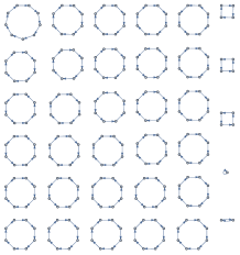
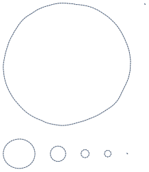
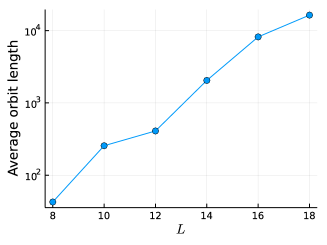
In this section, we provide further details on our implementation of the Bernoulli map. As discussed in the main text, the Bernoulli map cannot simply be given by the translation operator , Eq. (3), because the resulting map has orbits of length at most . The full set of orbits for a system with is shown in Fig. S1 (left). To make the map chaotic, we append a scrambler that acts on the end of the chain corresponding to the least significant bits of the point . The scrambler we use acts on the last three bits and can be represented by the cellular automaton
| (S6) |
The resulting chaotic map, , is a cellular automaton whose typical orbit lengths are exponential in , see Fig. S1 (right). An illustration of the full set of orbits for is shown in Fig. S1 (middle). Note that this scrambler does not preserve the length-two orbit onto which we are attempting to control the system—it allows the system to leave this orbit (by an exponentially small amount in a single time step) once it reaches it. In the context of the control transition, this feature actually slightly simplifies the numerical diagnosis of the transition. However, we could avoid it by replacing with a random automaton that maps . We have verified that the presence and location of the control transition are unaffected by this modification; our use of the scrambler (S6) is a choice of convenience.
S2.2 Control map: Controlled adder
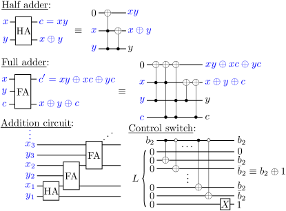
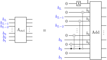
In this section we explain how the controlled adder , Eq. (7) in the main text, is constructed from local unitary gates. The adder consists of a few elementary building blocks, shown in Fig. S2. First, there is a half adder, which, given two bits and , outputs their sum mod 2, , and a carry bit which is set to if and only if . The half adder is built using one Toffoli and one CNOT gate. Next, there is a full adder, which takes in two bits and as well as a carry bit (assumed to be output by a previous addition operation) and outputs the sum and a new carry bit which is if and only if two or more of and are . This can be achieved with three Toffolis and two CNOTs. In order for these operations to be logically reversible (i.e., compatible with a unitary implementation), we need to augment the bits storing logical information (colored in blue in the figure) with input ancilla bits, which provide workspace for the circuit, and output garbage bits, whose values can be erased after performing the operation. The addition circuit is then obtained by forming a staircase of half and full adders, as shown at the bottom left of Fig. S2 suppressing the ancilla and garbage bits for clarity.
To construct the controlled addition circuit we need to prepend to the adder described above with a “control switch” circuit, whose purpose is to determine which binary fraction to add to the input bitstring . As noted in the main text, the fraction to be added is conditioned on the value of ; from Eq. (7), we see that it is given by , where is the logical complement of . This bitstring can be constructed from a register of ancillas initialized in using CNOT gates as shown at the bottom right of Fig. S2. The controlled adder then takes the form shown in Fig. S3.
S3 Krauss operator description
For the description in terms of quantum channels, we use the notation developed in the main text [specifically Eqs. (3-7)].
There are three Krauss operators:
| (S7) | ||||
describes the Bernoulli map applied with probability and represents the control map along with its two outcomes for the measurement: 0 and 1. Unitary control is applied, just as in the main text, when the outcome of measuring bit is 1. These satisfy , and the average density matrix satisfies is progressed from time to via
| (S8) |
Note that this is already distinct from the individual trajectories as we numerically simulate (which are characterized by products of chaotic evolution and the control operation). Entanglement data (ancilla, half-cut, etc.) cannot be directly computed with this expression, that still requires nonlinear observables in the density matrix of individual trajectories.
For purposes of applying the scrambler, we note that the density matrix can be written in tensor form
| (S9) |
where each line represents a qubit (1 to , reading left to right). The average of the Krauss map results reveal a connection between the quantum model and classical probability distributions due to
| (S10) |
where is the Haar measure over dimension 4 unitaries. Furthermore, if we put the density matrix through a dephasing channel to suppress off-diagonal contributions, we can write
| (S11) |
where all and are qubit -states. If we track the time evolution of (indicating an average over Haar distributed and a dephasing channel on ), then we get
| (S12) | ||||
In order to proceed, we want to find an expression for for an operator . We make a few definitions, using Eqs. (S1) and (S2) for notational help. First
| (S13) |
Notably, the inverse map , when it exists, is a set of two possibilities , for which satisfy . This lets us write
and furthermore
To connect this last expression with the classical map, call the operation which we combine with a scrambling operation which with equal probability takes to . In this way, and , and we therefore have
Taken together, we have an equation for the time evolution of probability distributions
| (S14) |
And finally, we need to be careful about taking the thermodynamic limit and relating it back to the Bernoulli map. In both cases the last bit is irrelevant and two bit strings and both will map to the same point in , yet they are summed over above. Therefore, we will identify these points such that where . In this limit, we can write the above expression
where we have lost the scrambler in the thermodynamic limit. Note that this defines the Frobenius-Perron operator (Eq. S3) defined in, for instance, Ref. [60] for and , proving that Krauss evolution of our density matrix is equivalent to classical evolution of probability distribution functions when we average over the Haar unitaries and use a dephasing channel.
S4 Additional data for the quantum model
S4.1 Order parameter and entanglement saturation
In Fig. S4, we plot the dynamics of for and for (averaged, as in the main text, over realizations) out to a time . For all values of we considered ( and are shown as representative values below, at, and above the control transition, respectively), the order parameter and half-cut entanglement entropy have saturated well before the final time in the simulation window. This justifies our use of times of order to probe properties of the steady state.
S4.2 System-size scaling of entanglement dynamics in the uncontrolled phase
In this section, we corroborate two statements made in the main text regarding the system-size dependence of the entanglement dynamics in the uncontrolled phase. The first statement, made below Eq. (4), is that the entanglement generated by the chaotic unitary saturates to a volume-law value in an time. Fig. S5(left) plots the realization-averaged entanglement entropy against at for . When is rescaled by the Page value, , for the entanglement entropy of a random state [68], we find that the dynamics collapse onto a single curve. This indicates that generates volume-law entanglement in an time, as claimed in the main text.
The second statement, made immediately before the Discussion and outlook section, is that volume-law entanglement can only develop at the transition if the FDW “sticks” to the left edge of the chain for at least an time. To simulate this scenario, we consider the realization-averaged dynamics at . Since a randomly chosen CB state has, with high probability, a FDW located near the left end of the chain, the average over realizations at probes what happens when the FDW is initialized near the left edge of the chain. We are then interested in the timescale for entanglement saturation starting from these initial conditions. Fig. S5(right) plots against at for . The rescaled data show a slight rightward drift of the entanglement saturation time as system size increases. This means that the entanglement saturation timescale can be lower-bounded by an value. Here, the low value of is chosen to encourage the FDW to stick to the left edge of the chain. However, at the transition , the dynamics of the FDW becomes an unbiased random walk. Thus, for the FDW to stick to the left edge of the chain for a time of at least requires the random walker to step to the left times, and the probability of this happening is exponentially small in .
S4.3 Fluctuations at the transition
The location of the control transition can also be probed by tracking the fluctuations of observables as a function of and . In Fig. S6, we show the standard deviation over realizations of the observables considered in Fig. 3 of the main text. For both the order parameter and the ancilla entanglement entropy , the fluctuations exhibit pronounced peaks near . For , the peak appears to drift towards and become sharper with increasing system size . For , the peak exhibits less drift in its position but still sharpens with increasing . Both datasets also exhibit a near collapse assuming the respective values of and determined in the main text.