Quantum memory at nonzero temperature in a thermodynamically trivial system

Abstract

Passive error correction protects logical information forever (in the thermodynamic limit) by updating the system based only on local information and few-body interactions. A paradigmatic example is the classical two-dimensional Ising model: a Metropolis-style Gibbs sampler retains the sign of the initial magnetization (a logical bit) for thermodynamically long times in the low-temperature phase. Known models of passive quantum error correction similarly exhibit thermodynamic phase transitions to a low-temperature phase wherein logical qubits are protected by thermally stable topological order. Here, in contrast, we show that constant-rate classical and quantum low-density parity check codes have no thermodynamic phase transitions at nonzero temperature, but nonetheless exhibit ergodicity-breaking dynamical transitions: below a critical nonzero temperature, the mixing time of local Gibbs sampling diverges in the thermodynamic limit. We conjecture that the circuit complexity of preparing extensive-energy states may diverge without crossing any thermodynamic transition. Fault-tolerant passive decoders, inspired by Gibbs samplers, may be amenable to measurement-free quantum error correction and may present a desirable experimental alternative to conventional quantum error correction based on syndrome measurements and active feedback.

1 Introduction

There is a deep relationship between error correction and thermodynamics. Data storage in magnetic devices (e.g. hard disk drives) relies on the fact that there are two stable magnetic configurations in a two-dimensional ferromagnet, such as the Ising model. Whether the spins point up or down determines whether a classical bit of information is 0 or 1. Crucially, the ferromagnetic phase is robust to thermal noise: at low temperatures, errors are passively corrected by the environment! The time until the stored data becomes corrupted is exponentially large in the system size Thomas (1989).

The simplest analogy to the above story for a quantum error-correcting code is the four-dimensional toric code Dennis et al. (2002). Intuitively, it corresponds to “two copies of the 2D Ising model”: since a quantum code must protect against both $X$ (bit-flip) and $Z$ (phase-flip) errors, half of the dimensions of the 4D toric code protect against each. Since the 2D Ising model exhibits a phase transition to ferromagnetism below a nonzero critical temperature Onsager (1944), the 4D toric code also has a nonzero critical temperature below which the thermal state has topological order Alicki et al. (2008). This topological order can protect logical quantum information forever in the thermodynamic limit, even in the presence of thermal noise. In other words, the 4D toric code is a passive quantum memory.

In all known examples of passive quantum error correction, there is a thermodynamic phase transition at nonzero temperature to a topologically ordered phase Alicki et al. (2008); Yoshida (2011); Hastings (2011); Brown et al. (2016); Liu and Lieu (2024). Such transitions are only known to exist in at least four spatial dimensions. Unfortunately, we live in three spatial dimensions. Therefore, many existing attempts to realize quantum error correction in experiment involve active decoding, where explicit measurements and feedback are necessary to protect quantum information. Yet many active decoders require global information about measurement outcomes, so the cost of performing such classical computations will increase as one builds ever-larger quantum computers. In contrast, a passively-decodable system corrects its own errors simply by thermalizing with a cold environment – far simpler, at least in principle, to realize experimentally.

Motivated by the above challenges, this paper addresses the question of whether quantum memory can exist without any thermal phase transitions to a topologically ordered phase. An answer to this question is important, both because it could constrain the space of quantum codes to explore in which passive error correction is even feasible, and because it is important to understand whether the limited nonlocality Xu et al. (2023); Hong et al. (2023) that can be realized in quantum hardware is sufficient to realize passive quantum error correction.

We will prove that a thermodynamic phase transition, at any nonzero temperature, is not necessary for finite-temperature self-correction in classical codes, and that a thermodynamic phase transition to a topologically ordered phase is not necessary for self-correction in quantum codes. Our analysis is of classical and quantum low-density parity-check (LDPC) codes Gallager (1962); Breuckmann and Eberhardt (2021). “Parity check” refers to the multi-bit generalizations of the ferromagnetic interactions in the Ising model; like in the Ising model, the interactions are frustration-free – they can all be satisfied simultaneously if all bits are in the 0 state (all spins up). Furthermore, the Hamiltonian of an LDPC code is $\mathsf{k}$-local – each term in the Hamiltonian only couples $\mathsf{k}=\mathrm{O}(1)$ degrees of freedom in the thermodynamic limit. However, there is no constraint on the physical range of these interactions when the interacting degrees of freedom are embedded in physical (three-dimensional) space. In fact, a typical LDPC code cannot be locally embedded in any finite dimension. The parity checks are “low-density” because they are $\mathsf{k}$-local, and each bit only participates in a finite number of parity checks. In this respect, these models are similarly “few-body” to the simpler Ising model, but can avoid stringent constraints on quantum error correction in few spatial dimensions Bravyi et al. (2010).

The “infinite-dimensionality” of LDPC codes naturally leads to two properties, each of which are critical for our story. Firstly, LDPC codes can be non-redundant – every single parity check is an independent constraint from the others. This is not true in the two-dimensional Ising model, where the product of interactions around a square plaquette is always $+1$. This non-redundancy ensures thermodynamic triviality of the random LDPC codes that we study. Secondly, a random LDPC code typically has rapidly growing energy barriers to small perturbations, implying that the ground states of its corresponding Hamiltonian reside in very deep local minima in the energy landscape. The large energy barriers to escape these local minima ensure that Gibbs sampling Metropolis et al. (1953); Hastings (1970), a specific kind of passive error correction, is capable of trapping the system near its starting state, which enables the eventual decodability of the information.

2 Classical codes

We first describe random classical LDPC codes, demonstrating both the simultaneous thermodynamic triviality and the self-correcting behavior. Informally, a classical LDPC code is a collection of $n$ physical bits $Z_{i}=\pm 1$ and $m$ parity checks of the form $S=\{s_{1},\ldots,s_{\Delta_{C}}\}$, which correspond to subsets of physical bits of size $\Delta_{C}$ in which the bits will interact via the following Hamiltonian:

$$\mathcal{H}=-\sum_{S=1}^{m}\prod_{j=1}^{\Delta_{C}}Z_{s_{j}}\,.$$ (1)

The $2^{k}\geq 2^{n-m}$ ground states of the above Hamiltonian are called logical codewords, generated by $k$ logical bits. Notice that one codeword ($\mathcal{H}=-m$) is the state $Z_{i}=1$ for all $i$. We restrict our focus to codes in which each bit $Z_{i}$ is contained in exactly $\Delta_{B}$ checks, and take $\Delta_{B}<\Delta_{C}.$ It is conventional in the coding literature to organize the data above as follows: letting $\mathbb{F}_{2}=\{0,1\}$, we consider an $\mathbb{F}_{2}$-valued $m\times n$ matrix $H$ such that

$$H_{Si}=\left\{\begin{array}[]{ll}1&\ \text{parity check $S$ contains bit $i$}\\ 0&\ \text{otherwise}\end{array}\right..$$ (2)

Defining the vector $\mathbf{z}\in\mathbb{F}_{2}^{n}$ with entries $z_{i}=\frac{1}{2}(1-Z_{i})$, we can write

$$\mathcal{H}=2|H\mathbf{z}|-m.$$ (3)

where $|\cdots|$ denotes the Hamming weight, or number of 1s, of any $\mathbb{F}_{2}$-valued vector. The code distance

$$d=\min_{\text{codeword }\textbf{x}\neq\mathbf{0}}|\mathbf{x}|$$ (4)

can be interpreted as the minimum number of bit flips to transition between codewords. These parameters are often conveniently packaged using the bracketed notation $[n,k,d]$.

Let us now review some key facts about randomly chosen LDPC codes $H$ subject to the above constraints (formal statements and proofs are relegated to Appendix A.1) Sipser and Spielman (1996); Richardson and Urbanke (2008): (1) almost surely as $n\rightarrow\infty$, for $\Delta_{B}\geq 3$, the rate of the code obeys

$$\frac{k}{n}=\mathfrak{r}=1-\frac{\Delta_{B}}{\Delta_{C}}\,.$$ (5)

In other words, the number of logical bits scales linearly with the system size $n$. (2) There exist O(1) numbers $\gamma,\eta>0$ such that for all $\mathbf{z}$ obeying $0<|\mathbf{z}|\leq\gamma n$, $|H\mathbf{z}|\geq\eta|\mathbf{z}|$. This property is called “linear confinement”: a continuous path of bit flips between codewords will necessarily cross an extensive energy barrier. Since this confinement holds up to $\gamma n$, the code distance must also scale linearly with the system size.

Using these facts and following Yoshida (2011); Freedman and Hastings (2013); Weinstein et al. (2019), we now show that this LDPC code has a trivial free energy in the thermodynamic limit. Observe that since $k=n-m$, $H$ has no left null vectors. Hence, given any $\mathbf{s}\in\mathbb{F}_{2}^{m}$, there are exactly $2^{k}$ candidate states $\mathbf{z}$ satisfying $\mathbf{s}=H\mathbf{z}$. It is then straightforward to evaluate

$$Z(\beta)=\sum_{\mathbf{z}}\mathrm{e}^{-\beta\mathcal{H}(\mathbf{z})}=\sum_{\mathbf{z}}\mathrm{e}^{-\beta(2|H\mathbf{z}|-m)}=2^{k}\sum_{\mathbf{s}}\mathrm{e}^{-\beta(2|\mathbf{s}|-m)}=2^{\mathfrak{r}n}(2\cosh\beta)^{(1-\mathfrak{r})n}.$$ (6)

The free energy density $f(\beta)=-n^{-1}\beta^{-1}\log Z(\beta)$ is clearly an analytic function for $0\leq\beta<\infty$, which means that there is no thermodynamic phase transition. Appendix A.2 provides another derivation of this fact based on generalizing classical Kramers-Wannier duality to generic parity-check codes with redundancy; yet another (quantum Kramers-Wannier) perspective on this result is found in Rakovszky and Khemani (2023).

Let us now study the dynamics of Gibbs sampling for this LDPC code. We consider the discrete-time Metropolis algorithm in which

$$\frac{\mathbf{P}[\mathbf{z}\rightarrow\mathbf{z}^{\prime}]}{\mathbf{P}[\mathbf{z}^{\prime}\rightarrow\mathbf{z}]}=\min\left(1,\mathrm{e}^{-\beta(\mathcal{H}(\mathbf{z}^{\prime})-\mathcal{H}(\mathbf{z}))}\right)\,.$$ (7)

We study $\mathsf{k}$-local dynamics in which $|\mathbf{z}-\mathbf{z}^{\prime}|$ is O(1) when $\mathbf{P}[\mathbf{z}\rightarrow\mathbf{z}^{\prime}]\neq 0$. Suppose that at time $t=0$, we start in the codeword $\mathbf{0}$. To bound the time it takes for the Gibbs sampler to destroy information, it suffices to bound the time it takes for the Gibbs sampler to reach a state $\mathbf{z}_{t}\in E$, where the “bottleneck” set $E$ consists of all $|\mathbf{z}_{t}|=\gamma n/2<d/2$. In thermal equilibrium, we observe that

$$\frac{\pi[E]}{\pi[\mathbf{0}]}\leq\mathrm{e}^{-\beta\eta\gamma n}\,{n\choose\gamma n/2}\lesssim\mathrm{e}^{-(2\beta\eta-\log(2/\gamma)-1)\gamma n/2}\,,$$ (8)

where $\pi$ denotes the Gibbs probability distribution: $\pi(\mathbf{x})=\mathrm{e}^{-\beta\mathcal{H}(\mathbf{x})}/Z(\beta)$. The Markov chain bottleneck theorem then shows that the Gibbs sampler, starting from codeword $\mathbf{0}$, will not reach the set $E$ before a typical time scale $t\gtrsim\mathrm{e}^{\mathrm{O}(n)}$ at low temperature. Below $E$, all states contain less than $d/2$ errors, and so are correctable in principle (under maximum-likelihood decoding). Specific decoders may require additional constraints; e.g., bit-flip can provably correct errors of weight up to $\gamma\eta\Delta_{B}^{-1}n$ for $\Delta_{B}\geq 5$ Sipser and Spielman (1996); these constant offsets do not change the overall behavior and can be accounted for by adjusting the definition of $E$. Since all transitions are equally probable at $T=\infty$ – the system will fully mix after we consider flipping each spin once – we deduce there must be a finite temperature $T_{\mathrm{c}}$ such that for $T<T_{\mathrm{c}}$, the system has (exponentially) slow mixing; our calculation provides a lower bound on $T_{\mathrm{c}}$.

Figure 1: A snapshot of the energy landscape of a typical good classical LDPC code is depicted. Extensively deep minima separate codewords and low-energy configurations consisting of single flipped parity checks. Below a critical temperature, the Gibbs sampler becomes trapped inside its initial minimum and is unable to explore the full state space, preventing the system from reaching thermal equilibrium.

How is it possible to have thermodynamic triviality, while the Gibbs sampler simultaneously protects a codeword? The answer lies in the peculiar energy landscape of these LDPC codes, illustrated in Figure 1. Locally near each codeword, the linear confinement property guarantees a very deep minimum in the energy landscape. If we could restrict $Z(\beta)$ to only count states $\mathbf{x}$ with $|\mathbf{x}|\leq\gamma n$, the Helmholtz free energy would exhibit a phase transition: above a critical temperature, the typical state would have $|\mathbf{x}|/n\rightarrow\gamma$, while below it the typical state is much closer to the codeword $\mathbf{0}$, as guaranteed by (8). In reality however, $Z(\beta)$ counts the whole state space, and when we look beyond the local landscape near a given codeword, we see a “swamp” of many very deep minima, some of which contain other codewords, but far more of which contain “sick” configurations where, e.g., a single parity check is flipped Rakovszky and Khemani (2023, 2024). Indeed, we have seen that there must exist a state with a single flipped parity-check since $H$ has no left null vectors; at the same time, such a state $\mathbf{x}$ obeys $|\mathbf{x}|=\mathrm{O}(n)$, and it too will have an extremely deep energy well where the Gibbs sampler would be stuck. The key point is the conceptual distinction between static equilibrium and dynamical equilibration – the thermodynamic free energy detects all of the exponentially many fake codewords, while the Gibbs sampler is stuck near whichever minimum it starts in.

To have a genuine thermodynamic phase transition, redundancy must be added to the parity checks, such that the sick configurations of Figure 1 gain finite energy density. The energetic suppression of these sick configurations is encapsulated by a closely related property to confinement known as soundness, which stipulates that small energy violations can always be produced by small errors. Note that the LDPC codes we have discussed are confined but not sound due to the low-energy sick configurations. The 2D Ising model, on the other hand, is both confined and sound. The intimate relationship between redundancy and soundness has been studied in the context of locally testable codes (LTCs) Ben-Sasson et al. (2009), in which one can reliably determine whether a state is a codeword by only querying a small number of physical bits. “Good” locally testable codes with constant rate, constant relative distance and constant query complexity ($c^{3}$-LTCs) have recently been found Panteleev and Kalachev (2022); Lin and Hsieh (2022); Dinur et al. (2022a). While redundancy and soundness is a feature of these codes, we have seen that they are unnecessary to have ergodicity-breaking at low temperatures.

3 Quantum codes

We now turn to a summary of analogous results for quantum LDPC codes Breuckmann and Eberhardt (2021) of the Calderbank-Shor-Steane (CSS) type Calderbank and Shor (1996); Steane (1996). We begin with two classical LDPC codes with $M\times N$ parity-check matrices $H_{X}$ and $H_{Z}$ respectively, subject to the orthogonality constraint $H_{X}H_{Z}^{\mathrm{T}}=0$ (here the matrix multiplication uses $\mathbb{F}_{2}$ algebra). For each row of $H_{X}$, we define an $X$-stabilizer which is the product of a Pauli $X$ acting on each qubit in the parity check; for $H_{Z}$, the stabilizers consist of Pauli $Z$s. The orthogonality constraint above ensures that the $X$-type and $Z$-type stabilizers commute, and hence can be simultaneously diagonalized. The $+1$ eigenspace of all stabilizers forms the Hilbert space of logical qubits, or codewords. Logical $X$/$Z$ operators correspond to products of Pauli $X$/$Z$ that commute with all $Z$/$X$-type stabilizers; if we have $K$ of each, then the code stores $K$ logical qubits. The code distance $D$ is the length of the smallest such logical operator. We define a quantum Hamiltonian to be the sum over these stabilizers:

$$\mathcal{H}=-\sum_{\text{$X$-stabilizer }S}\,\prod_{i\in S}X_{i}\;-\sum_{\text{$Z$-stabilizer }S}\,\prod_{i\in S}Z_{i}\,.$$ (9)

It is quite challenging to find a quantum LDPC code of $N$ qubits in which the code distance $D=\mathrm{O}(N)$, although recently some have been found Panteleev and Kalachev (2022); Leverrier and Zémor (2022); Dinur et al. (2022b). To keep the discussion as transparent as possible, we will instead discuss the simplest family of quantum LDPC codes, called hypergraph product (HGP) codes Tillich and Zemor (2014). HGP codes are formed by a graph product of two classical codes, each of which we take to be a good random LDPC code of the kind previously mentioned with parameters $[n,k=\mathrm{O}(n),d=\mathrm{O}(n)]$. The HGP construction is illustrated in Figure 2, while explicit formulas are relegated to Appendix B.1. One can prove the following important facts about such random HGP codes, each of which holds almost surely in the thermodynamic limit: (1) they are constant-rate codes with $N=n^{2}+(n-k)^{2}$, $D=d$, and $K/N=\mathfrak{r}^{2}$, with $\mathfrak{r}$ inherited from the classical LDPC code and given in (5). There are $M=n(n-k)$ checks of both $X$ and $Z$ type, and there are no redundant checks. (2) Like classical LDPC codes, they exhibit linear confinement Leverrier et al. (2015): given any binary string $\mathbf{x}\in\mathbb{F}^{N}_{2}$ corresponding to an $X$-type or $Z$-type error with weight $|\mathbf{x}|\leq\gamma n$, we have $|H_{X}\mathbf{x}|,|H_{Z}\mathbf{x}|\geq\eta|\mathbf{x}|$ for some $\eta=\mathrm{O}(1)$. (3) Every stabilizer involves exactly $\Delta_{B}+\Delta_{C}$ qubits, and each qubit is involved in at most $\Delta_{C}$ $X$-stabilizers and $\Delta_{C}$ $Z$-stabilizers.

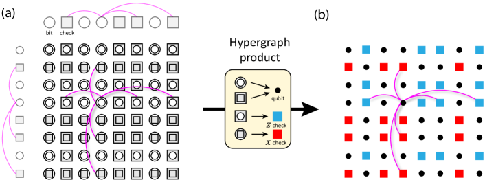
Figure 2: The hypergraph product construction is illustrated. (a) The Euclidean graph product is taken between the Tanner graph of a classical parity-check code and itself, producing four types of vertices. (b) The hypergraph product maps the four types of vertices in the product graph to qubits, $X$-checks and $Z$-checks, thus producing a quantum CSS code. The interactions in the hypergraph product code resemble those of its classical input code (in magenta).

With these facts in hand, it is straightforward to show that there is no finite-temperature thermodynamic phase transition in such models. The proof is exactly analogous to that of the classical models: as the stabilizers mutually commute, we can evaluate the partition function in subspaces of fixed stabilizer eigenvalues, each of which has Hilbert space dimension $2^{K}$. Therefore, since the stabilizers are linearly independent,

$$Z(\beta)=\mathrm{tr}\left(\mathrm{e}^{-\beta\mathcal{H}}\right)=2^{K}\left(2\cosh\beta\right)^{N-K}.$$ (10)

The free energy density $F(\beta)=-N^{-1}\beta^{-1}\log Z$ is again an analytic function for $0\leq\beta<\infty$, so there is no thermodynamic phase transition.

However, once again, Gibbs sampling is exponentially slow below a critical temperature. Since the Hamiltonian $\mathcal{H}$ is a sum of independent $X$-checks and $Z$-checks, our quantum Gibbs sampler will simply measure the set of e.g. $X$-stabilizers containing a given qubit $i$, and with suitable probability analogous to (7), apply Pauli $Z_{i}$ to the state afterwards. We prove in Appendix B.3 that the time it takes to reach a state for which known decoders might fail to decode is $t\gtrsim\mathrm{e}^{\mathrm{O}(\sqrt{N})}$ for $\beta$ above some critical temperature. The proof strategy is similar to the one for classical LDPC codes, but is slightly more involved as for HGP codes we do not have $D\sim N$. We use the fact that errors typically form disconnected clusters, and these clusters rarely conspire to fool an eventual decoder. States with such adversarial clusters are, at low temperature, found in the Gibbs ensemble with probability $\mathrm{e}^{-\mathrm{O}(\sqrt{N})}$, and so it will take us a long time to reach one. This is analogous to Peierls’s argument that the two-dimensional Ising model is ordered at low temperatures because we are unlikely to find long domain walls Peierls (1936). Numerical simulations confirming the slow dynamics are presented in Appendix C.

We understand the existence of this ergodicity-breaking in Gibbs sampling in exactly the same way as illustrated for classical LDPC codes. The quantum LDPC codes have a very complex energy landscape, such that the Gibbs sampler will get stuck in a very deep energy minimum for exponentially long times; in contrast, the thermodynamics is sensitive to the “swamp” of exponentially many deep local minima corresponding to very large errors that flip few parity checks. A thermal phase transition requires redundancy which our HGP codes do not have. Numerical simulations had previously suggested that passive decoding might be possible even above a nonzero critical temperature for topological order Hastings et al. (2014); we stress that in our construction, the model is completely thermodynamically trivial. Nonvanishing energy barriers have been the primary features of Haah’s cubic code Haah (2011) and welded codes Michnicki (2014). Nonetheless, it has been shown that the lifetime of logical information in these codes is finite at any positive temperature due to entropic effects Bravyi and Haah (2013); Siva and Yoshida (2017).

We have shown that passive error correction is possible for quantum LDPC codes. Previous work has shown that such codes have good greedy decoders Leverrier et al. (2015) and that single-shot quantum error correction Bombin (2015); Campbell (2019) – where a single round of noisy syndrome measurement suffices to suppress errors – is achievable Quintavalle et al. (2021); Fawzi et al. (2018); Gu et al. (2023). Passive error correction is arguably even more desirable than single-shot error correction, as the single-shot decoder may nevertheless require global information as part of the decoding, whereas by construction the Gibbs sampling dynamics described above does not. In other words, an autonomous machine can detect and correct quantum errors in a memoryless way. Below a physical error threshold, the logical error rate can be suppressed to arbitrarily low levels by increasing the size of the system. We emphasize that since the quantum LDPC codes have a nonvanishing rate in the thermodynamic limit, the overhead (number of physical qubits per logical qubit) remains constant.

4 Measurement-free quantum error correction

Due to the spatial non-locality of the $\mathsf{k}$-local LDPC codes, it may be challenging to simply “let them thermalize” with a cold environment to build a quantum memory. Nevertheless, let us now explain a very useful and practical alternative, based on “measurement-free quantum error correction” (MFQEC) Ahn et al. (2002); Sarovar and Milburn (2005), in which the user can only apply unitary gates and a specific “reset” dissipative quantum channel to the physical qubits. More formally, given density matrix $\rho$ for the physical qubits, we can only apply $\rho\rightarrow U\rho\,U^{\dagger}$ for unitary $U$, or apply $\rho\rightarrow R_{i}[\rho]$ where channel $R_{i}$ acts on single qubit $i$ as $R_{i}[\rho_{i}]=|0\rangle\langle 0|$; here we defined $Z|0\rangle=|0\rangle$. In addition to these processes, we also have errors occurring in the system, which we take to be independent and few-qubit, albeit occurring at a constant rate per qubit. The strategy behind MFQEC is to introduce ancilla qubits in addition to the $N$ physical qubits of the code. At the beginning of each error correction round, we apply the reset channel such that the state of the system is $|\psi_{\mathrm{total}}\rangle=|\psi_{\mathrm{phys}}\rangle\otimes|\mathbf{0}\rangle_{\mathrm{anc}}$. The role of the ancilla qubits is best understood as storing the measurement outcomes that would have occurred in conventional quantum error correction, which proceeds by measuring all the parity-checks (syndromes) and deducing where errors occurred based on these outcomes. In MFQEC, rather than measuring a stabilizer, we instead apply CNOT gates to encode the parity of the stabilizer into the state of the ancilla qubit (so long as CNOT is applied error-free). Then, we apply gates to the code conditioned on the state of the ancilla – i.e., we error correct based on syndromes. Using Stinespring’s formulation of measurement Stinespring (1955); Friedman et al. (2022) wherein measurement outcomes are stored in auxiliary qubits in Hilbert space such that the measurement process becomes unitary, a round of MFQEC is mathematically equivalent to a round of conventional QEC.

Still, from an experimental perspective, MFQEC can be highly desirable. Once we have a memoryless local decoder, implementing it via MFQEC will only require a constant number of ancilla bits per physical bit to store the measurement outcomes necessary for error correction. For one thing, once the error correction has been applied, we no longer need memory of those measurement outcomes, and so the ancilla qubits can be reset. More importantly, and in contrast to single-shot decoding strategies that use global syndrome information, we only need a finite-depth circuit to implement the passive feedback via MFQEC.

Let us illustrate how to perform MFQEC for our Gibbs sampler, using $\leq 3$-qubit gates, and reset. For simplicity, we focus only on the step that “corrects” $X$ errors on qubit $i$, as the story is analogous for $Z$ errors and other qubits. Let ancilla qubits $a_{1},\ldots,a_{\Delta_{C}}$ store the “measurement outcomes” for the $\Delta_{C}$ $Z$-checks $C_{1},\dots,C_{q}$ containing physical qubit $i$. The first step of MFQEC is to apply the unitary

$$U_{1}=\prod_{q=1}^{\Delta_{C}}\prod_{j\in\mathrm{supp}(C_{q})}\mathsf{CNOT}_{j\rightarrow a_{q}},$$ (11)

where $\mathsf{CNOT}_{i\rightarrow j}=\frac{1+Z_{i}}{2}+\frac{1-Z_{i}}{2}X_{j}$. In the second step, we apply the $\mathsf{SORT}_{\Delta_{C}}$ channel, which shuffles the ancilla qubits such that the zeros are to the left and the ones are to the right. We provide an implementation for $\mathsf{SORT}$ in Appendix D using $\leq 3$-qubit gates and reset. In order to realize a perfect Gibbs sampler, we apply a coherent gate that implements the following controlled-unitary using one additional ancilla qubit $c$, which is again initialized in state $|0\rangle$:

$$U_{2}=\left[\prod_{j=1}^{\Delta_{C}}\mathrm{e}^{\mathrm{i}\theta_{j}\big{(}1-Z_{a_{j}}\big{)}X_{i}Z_{c}/2}\right]X_{c}\,,$$ (12)

where we choose each angle $\theta_{j}$ such that

$$\sin^{2}\left(\sum_{k=j}^{\Delta_{C}}\theta_{k}\right)=\mathrm{e}^{2\beta\min(0,\Delta_{C}-2j)}\,.$$ (13)

With these rotation angles, the cumulative probability of applying $X_{i}$ matches those precisely set by the Metropolis algorithm. In particular, we always apply feedback if doing so reduces the energy, i.e. the number of violated parity checks; however, we also introduce our own errors with a small probability. Once this is done, we apply the reset channel to all ancilla qubits. Tracing out $c$ gives us a reduced density matrix that contains superpositions of modes rotated by $\pm\theta$, which is the same as an incoherent Pauli $X$ error with probability $\sin^{2}\theta$.

Given the Gibbs sampler above, we can readily convert it into a genuine passive decoder in the presence of unwanted errors. If, for example, there are single-qubit incoherent $X$ errors that occur at rate $\gamma$, then we modify (13) to

$$\sin^{2}\left(\sum_{k=j}^{\Delta_{C}}\theta_{k}\right)=\left(\mathrm{e}^{2\beta\min(2j,\Delta_{C})}-1\right)\gamma.$$ (14)

Combining our modified sampler with the intrinsic errors reproduces a perfect Gibbs sampler, which we have seen is a passive quantum memory.

As a practical matter, we expect that our Gibbs sampler can be modified to never introduce unwanted errors, and that the lifetime of logical information should only increase. This also simplifies the circuit above (see Appendix D). More importantly, we note that our protocol is fault-tolerant: it works even if there is noise during the MFQEC process itself. As an explicit example of this, we show in Appendix D that if the overall single-qubit error rates are sufficiently small (but finite), it is possible to Gibbs sample in the presence of errors during the MFQEC circuit.

5 Outlook

We have proved that random classical and quantum LDPC codes are constant-rate quantum memories, in which $N$ physical (qu)bits which undergo local, memoryless, time-reversal-symmetric Gibbs-sampling dynamics at low temperature, thus protecting $\mathrm{O}(N)$ logical (qu)bits for infinite time in the thermodynamic ($N\rightarrow\infty$) limit. This property holds even as the codes are thermodynamically trivial – they have no thermodynamic phase transitions at nonzero temperature. Our result provides a deeper understanding of the surprising connections between statistical physics and error correction: contrary to prior intuition, thermal phase transitions are unnecessary for passive error correction, which can be performed by sampling the thermal Gibbs state, in either classical or quantum codes.

The self-correcting capability of LDPC codes has a number of intriguing implications and connections with other research thrusts in physics. The LDPC codes we described in this paper are arguably the simplest (albeit high-dimensional) examples of models exhibiting dynamical state/Hilbert space shattering in the thermodynamic limit: the system is dynamically trapped in an exponentially small region of the state space, even in the absence of any protecting symmetry or even simply frustration or Hilbert space constraints. Our result thus makes a sharp connection between error-correcting codes and recent models of ergodicity breaking in statistical physics Sala et al. (2020); Khemani et al. (2020); Hart and Nandkishore (2022); Stephen et al. (2024); Stahl et al. (2023); Han et al. (2024).

Since no locally-testable good quantum LDPC codes ($c^{3}$-qLTCs) are known yet, we conjecture that the non-extensive redundancy of our quantum hypergraph product codes is also shared by the existing good (constant-rate $K\sim N$ and linear-distance $D\sim N$) quantum LDPC codes Panteleev and Kalachev (2022); Leverrier and Zémor (2022); Dinur et al. (2022b). If true, our proof immediately generalizes to such models, and implies that circuit complexity of preparing states is not a universal characteristic of a thermodynamic phase – namely, that the circuit depth needed to prepare a state at various energy densities will transition from finite to infinite (in the thermodynamic limit) without crossing any thermal phase transition. After all, such codes have the no-low-energy-trivial-states (NLTS) property Freedman and Hastings (2013); Anshu et al. (2023) – arbitrary eigenstates of a Hamiltonian, up to a finite energy density, are topologically ordered: they cannot be constructed from a product state via a finite-depth circuit. Nonetheless, extensive redundancy is required for phase transitions at nonzero temperature! This conclusion is rather surprising: we currently define two pure states to be in the same phase only when they are related by a finite-depth unitary circuit Chen et al. (2010). The situation for mixed states is less clear, see Sang et al. (2023) for recent developments. Evidently, NLTS would thus reveal two mixed states in the same thermodynamic phase which simultaneously violate the above criterion. A better understanding of such a discrepancy is an interesting problem for the future.

Lastly, let us remark on the relevance of our results for neutral atom quantum computing Saffman et al. (2010); Kaufman and Ni (2021); Cong et al. (2022); Bluvstein et al. (2022); Jenkins et al. (2022); Bluvstein et al. (2023). (1) In this platform, the reset operation can be about 100 times faster than mid-circuit measurement and feedback Lis et al. (2023); Norcia et al. (2023); Huie et al. (2023). The circuit depth needed for MFQEC is a constant-factor $\lesssim 3$ larger than that needed for QEC based on mid-circuit measurement and feedback (at the cost of adding $\mathrm{O}(N)$ extra ancillas), so we expect that a passive decoder would operate faster. The primary disadvantage of the passive decoder – a possibly slow implementation of nonlocal atomic motion – would be just as problematic for the syndrome measurements themselves. (2) HGP codes are well-suited to the hardware capabilities of atom arrays Xu et al. (2023); Hong et al. (2023), in which acousto-optical deflectors can perform row and column permutations nonlocally in space relatively quickly (at least, for near-term system sizes). Hence, spatial nonlocality of the LDPC code is not necessarily prohibitive of its implementation in the absence of a large quantum-repeater network Fowler et al. (2010); Azuma et al. (2023). (3) Neutral atom platforms have increased their number of physical qubits Bluvstein et al. (2023) more rapidly than other platforms, which suggests that the additional ancilla qubit overhead for the fastest passive decoding strategy is less burdensome. Lastly, our numerical simulations suggests that the rigorous bounds on threshold error rates are far more stringent than needed in practice. While a detailed cost-benefit analysis of measurement-free vs. syndrome-based error correction in this platform remains to be performed, and the precise implementation of any optimal (possibly hybrid passive/active) error-correcting protocol remains to be found, we are optimistic that passive decoding of LDPC-based quantum memories is particularly suitable for neutral atom platforms and can play an important role in realizing fault-tolerant quantum computers in the future.

Note added.— In forthcoming work, other authors have independently investigated thermodynamics vs. dynamics in LDPC codes Breuckmann et al. (to appear).

Appendix A Classical LDPC codes

A.1 Linear parity-check codes

A classical linear code $\mathcal{C}$ encodes $k$ logical bits inside $n$ physical bits using a $m\times n$ parity-check matrix with binary $\mathbb{F}_{2}\simeq\mathbb{Z}_{2}$ coefficients (written as $H\in\mathbb{F}_{2}^{m\times n}$). From $H$ we can construct a $k\times n$ generator matrix $G$ which spans the codespace $\ker(H)$, the set of right binary null vectors, or codewords, of $H$. $\ker(H)$ is a binary vector space of dimension $k\geq 0$ – we say that $k$ is the number of logical bits stored in the code. Defining the Hamming weight of a binary vector $\mathbf{x}\in\mathbb{F}^{n}_{2}$ as the number of nonzero entries, and denoting this number with $\absolutevalue{\mathbf{x}}$, we say that the code distance $d$ is defined as

$$d=\min_{\mathbf{x}\in\mathcal{C}\backslash\mathbf{0}}\absolutevalue{\mathbf{x}}\,.$$ (15)

The code parameters are often packaged using the bracketed notation $[n,k,d]$. By the rank-nullity theorem, the parity-check matrix $H$ will have $r$ linearly independent nontrivial left null vectors, where

$$r=m-n+k\geq 0.$$ (16)

If $r=0$, corresponding to a full-rank parity-check matrix $H$, we say that the code is non-redundant, and the equation

$$\mathbf{s}=H\mathbf{e}$$ (17)

has $2^{k}$ solutions $\mathbf{e}$, which differ by logical codewords (alternatively, the solution is unique in $\mathbb{Z}_{2}^{n}/\ker(H)$).

Let $B$ be the vector space of all physical bits, with $|B|=n$, and let $S$ be the vector space of all parity checks with $|S|=m$. One can form a 3-term chain complex

$$B\xlongrightarrow{H}S\xlongrightarrow{M}R\,,$$ (18)

where $R$ denotes the spaces of redundancies, and the boundary maps $H$ and $M$ are the parity-check matrix and the matrix which collects its left null vectors respectively. These left null vectors can be interpreted as parity constraints amongst the checks themselves, commonly referred to as metachecks. $R$ is defined as the vector space of metachecks.

We say that $H$ is $(\Delta_{B},\Delta_{C})$ LDPC (low-density parity-check) if the maximum Hamming weights of its rows and columns are $\Delta_{C},\Delta_{B}=O(1)$ respectively. In other words, every check acts on a constant number of physical bits, and every bit only participates in a constant number of checks. If both $k=\Theta(n)$ (constant rate) and $d=\Theta(n)$ (linear distance), then we say the code is “good”. For most of this paper, our interest is on LDPC codes, although some of the results we derive below are not specific to this case.

Good LDPC codes are often constructed from regular, bipartite expander graphs; such codes are commonly referred to as expander codes Gallager (1962); Sipser and Spielman (1996). We now review some relevant results about expander codes.

Definition A.1 (Bipartite expansion Sipser and Spielman (1996)).

Given a regular bipartite graph $\mathcal{G}=(B\cup C,E)$ with uniform left-right degrees $\Delta_{B},\Delta_{C}=O(1)$, we say that $\mathcal{G}$ is $(\gamma,\delta)$ left-expanding if for any subset $B^{\prime}\subset B$ with volume $\absolutevalue{B^{\prime}}\leq\gamma n$, the size of its boundary $\partial B^{\prime}\subset C$ obeys

$$\absolutevalue{\partial B^{\prime}}\geq(1-\delta)\Delta_{B}\absolutevalue{B^{\prime}}\,.$$ (19)

The definition of right-expansion follows analogously by swapping the roles of $B$ and $C$. If $\mathcal{G}$ is both left and right-expanding, then we simply say it is a $(\gamma,\delta)$ expander.

We can define a $(\Delta_{B},\Delta_{C})$-LDPC expander code $\mathcal{C}_{\mathcal{G}}$ by identifying the left-nodes $B$ with physical bits and the right-nodes $C$ with parity checks. The parity-check matrix $H$ is given by the bipartite adjacency matrix of $\mathcal{G}$. Using the above definition of a bipartite expander, one can immediately derive lower bounds on the code parameters of $\mathcal{C}$.

Theorem A.2 (Constant rate Gallager (1962)).

If $\Delta_{B}<\Delta_{C}$, then the rate of $\mathcal{C}_{\mathcal{G}}$ is at least

$$k/n\geq 1-\Delta_{B}/\Delta_{C}\equiv\mathfrak{r}_{\rm des}\,,$$ (20)

where $\mathfrak{r}_{\rm des}\equiv 1-\Delta_{B}/\Delta_{C}$ is called the design rate.

Proof.

Let $n=\absolutevalue{B}$ and $m=\absolutevalue{C}$ be the number of bits and checks respectively. The number of edges emanating out of all bits and checks must be equal for a bipartite graph, so we have that $n\Delta_{B}=m\Delta_{C}$. Since the rank of $H$ is upper-bounded by the number of rows $m$, by the rank-nullity theorem, we conclude that

$$\frac{k}{n}\geq\frac{n-m}{n}=1-\frac{m}{n}=1-\frac{\Delta_{B}}{\Delta_{C}}=\mathfrak{r}_{\rm des}\,.$$ (21)

∎

Lemma A.3 (Unique neighbor expansion Sipser and Spielman (1996)).

Suppose $G$ is left-expanding with $\delta<1/2$. Then for any subset of bits $B^{\prime}\subset B$ with size $\absolutevalue{B^{\prime}}\leq\gamma n$, the number of unique neighbors $\partial_{u}B^{\prime}\subset\partial B^{\prime}\subset C$, checks which have only one edge connecting to $B^{\prime}$, is at least

$$\absolutevalue{\partial_{u}B^{\prime}}\geq\Delta_{B}(1-2\delta)\absolutevalue{B^{\prime}}\,.$$ (22)

Proof.

Since $\mathcal{G}$ is regular, the number of edges emanating out of $B^{\prime}$ is $\Delta_{B}B^{\prime}$. Since $\mathcal{G}$ is also left-expanding with $\delta<1/2$, from (19) we have $\absolutevalue{\partial B^{\prime}}\geq(1-\delta)\Delta_{B}\absolutevalue{B^{\prime}}$ for $\absolutevalue{B^{\prime}}\leq\gamma n$. Each of the neighboring checks in $\partial B^{\prime}$ must be connected by at least one edge from the definition of being a neighbor, so the number of remaining edges is $\Delta_{B}B^{\prime}-(1-\delta)\Delta_{B}\absolutevalue{B^{\prime}}=\delta\Delta_{B}\absolutevalue{B^{\prime}}$. By the pigeon-hole principle, the number of neighboring checks connected by only one edge is at least $\absolutevalue{\partial_{u}B^{\prime}}\geq(1-\delta)\Delta_{B}\absolutevalue{B^{\prime}}-\delta\Delta_{B}\absolutevalue{B^{\prime}}=\Delta_{B}(1-2\delta)\absolutevalue{B^{\prime}}>0$. ∎

We see that if $\mathcal{G}$ exhibits sufficient expansion $(\delta<1/2)$, then large subsets of bits will be connected to large amounts of unique checks. The above notion of unique neighbor expansion immediately gives us a confinement property Quintavalle et al. (2021), which loosely speaking, says that small errors produce small syndromes. We can quantify the confinement of expander codes as follows.

Corollary A.4 (Linear confinement).

Suppose $\mathcal{G}$ is left-expanding with $\delta<1/2$. Then for any error $\mathbf{e}$ with weight $\absolutevalue{\mathbf{e}}\leq\gamma n$, the weight of its syndrome $\mathbf{s}(\mathbf{e})=H\mathbf{e}$ is at least

$$\absolutevalue{\mathbf{s}(\mathbf{e})}\geq\Delta_{B}(1-2\delta)\absolutevalue{\mathbf{e}}\,.$$ (23)

We note that the linear confinement property of expander codes has a physical interpretation in terms of macroscopic energy barriers between codeword states of the corresponding Hamiltonian. We can also use Lemma A.3 to derive a lower bound on the code distance.

Theorem A.5 (Linear distance Sipser and Spielman (1996)).

If $G$ is left-expanding with $\delta<1/2$, then the code distance of $\mathcal{C}_{\mathcal{G}}$ is at least

$$d\geq 2\gamma(1-\delta)n\,.$$ (24)

Proof.

We will prove by contradiction that the weight of any nonzero codeword must be at least $2\gamma(1-\delta)n$. Suppose we have a codeword $\mathbf{x}\neq\mathbf{0}$ whose nonzero support is the set $\mathrm{supp}(\mathbf{x})=B^{\prime}\subset B$ with $\absolutevalue{B^{\prime}}<2\gamma(1-\delta)n$. If $\absolutevalue{B^{\prime}}\leq\gamma n$ then Lemma A.3 tells us that we have at least $\absolutevalue{\partial_{u}B^{\prime}}\geq\Delta_{B}(1-2\delta)\absolutevalue{B^{\prime}}$ unique neighbors, and hence unsatisfied checks, and so it is impossible for $\mathbf{x}$ to be a codeword. Now assume $\absolutevalue{B^{\prime}}>\gamma n$. Partition $B^{\prime}$ into a subset $S\subset B^{\prime}$ of size $\absolutevalue{S}=\gamma n$ and its complement $\bar{S}\equiv B^{\prime}\,\backslash\,S\subset B^{\prime}$ of size $\absolutevalue{\bar{S}}<\gamma(1-2\delta)n$. Lemma A.3 tells us that $S$ has at least $\absolutevalue{\partial_{u}S}\geq\Delta_{B}(1-2\delta)\absolutevalue{S}=\gamma\Delta_{B}(1-2\delta)n$ unsatisfied checks. On the other hand, there are at most $\Delta_{B}\absolutevalue{\bar{S}}<\gamma\Delta_{B}(1-2\delta)n\leq\absolutevalue{\partial_{u}S}$ edges emanating out of the complement $\bar{S}$. So there are not enough edges in $\bar{S}$ to pair up all of the unsatisfied checks of $S$. As a consequence, $\mathbf{x}$ will violate at least one check, which contradicts the assumption that $\mathbf{x}$ is a codeword. Thus we require $\absolutevalue{\mathbf{x}}\geq 2\gamma(1-\delta)n$ for all nonzero codewords $\mathbf{x}\in\ker(H)$, and so by definition, the code distance satisfies (24). ∎

Now that we have reviewed how bipartite expander graphs can lead to good LDPC codes, the problem boils down to constructing bipartite graphs with the required expansion properties. Explicit constructions with $\delta<1/2$ are notoriously difficult; see, however, Capalbo et al. (2002). Nonetheless, if one randomly constructs a bipartite graph using probabilistic methods, it will often exhibit the required expansion with high probability. We focus on regular ensembles, where the target degree distributions are singular around $\Delta_{B},\Delta_{C}$; we call such an ensemble the $(\Delta_{B},\Delta_{C})$-LDPC ensemble. The success of the random construction can be quantified by the following result.

Theorem A.6 (Random expansion; Theorem 8.7 of Richardson and Urbanke (2008)).

Let $\mathcal{G}$ be chosen uniformly at random from the $(\Delta_{B},\Delta_{C})$-LDPC ensemble with fixed $n$ and $\Delta_{B}>1/\delta$. Let $\gamma_{\rm max}>0$ be the solution of the equation

$$\frac{\Delta_{B}-1}{\Delta_{B}}h_{2}(\gamma_{\rm max})-\frac{1}{\Delta_{C}}h_{2}\big{(}\Delta_{C}\gamma_{\rm max}(1-\delta)\big{)}-\Delta_{C}\gamma_{\rm max}(1-\delta)\,h_{2}\left(\frac{1}{\Delta_{C}(1-\delta)}\right)=0\,,$$ (25)

where $h_{2}(x)\equiv-x\log x-(1-x)\log(1-x)$ is the binary entropy function. Then for $0<\gamma<\gamma_{\rm max}$ and $\alpha\equiv\Delta_{B}\delta-1$,

$$\mathbf{P}\left\{\text{$\mathcal{G}$ \emph{is a} $(\gamma,\delta)$ \emph{left-expander}}\right\}=1-O(n^{-\alpha})\,.$$ (26)

The analogy for right-expansion follows from switching the roles of $B\leftrightarrow C$.

As a consequence, simply constructing a random parity-check matrix $H$ with target column and row weights $3\leq\Delta_{B}<\Delta_{C}$ will result in a good LDPC code with probability 1 in the thermodynamic limit $n\rightarrow\infty$. We note that in practice, the code distances associated with these codes are often much higher than the theoretical guarantees. Theorem A.2 provides a lower bound on the rate of the code. The next result shows that the random construction produces codes whose rate is within $O(1/n)$ of the lower bound with high probability:

Lemma A.7 (Rate approaches design rate; Lemma 3.27 of Richardson and Urbanke (2008)).

Let $\mathcal{C}$ be chosen uniformly at random from the $(\Delta_{B},\Delta_{C})$-LDPC ensemble with fixed $n$ and $2\leq\Delta_{B}<\Delta_{C}$. Let $\mathfrak{r}_{\rm des}=1-\Delta_{B}/\Delta_{C}$ denote the design rate. Then the actual rate $\mathfrak{r}\equiv k/n$ satisfies

$$\mathbf{P}\left\{n\mathfrak{r}=n\mathfrak{r}_{\rm des}+\nu\right\}=1-o_{n}(1)\,,$$ (27)

where $\nu=1$ if $\Delta_{B}$ is even and $\nu=0$ otherwise.

The extra constant $\nu=0,1$ comes from the fact that when $\Delta_{B}$ is even, there is an automatic redundancy coming from the constraint that the sum of all checks (mod 2) is zero. Lemma A.7 asserts that all other checks are linearly independent with high probability.

An interesting property of non-redundant codes is that all $2^{m}=2^{n-k}$ syndromes have a corresponding physical error up to the action of a codeword. To see this fact, first note that $H$ has full rank because all its rows are linearly independent. Because row and column ranks are equal, we can thus select $m=n-k$ linearly independent columns of $H$ to form a new, invertible $m\times m$ matrix $\tilde{H}$. For any syndrome $\mathbf{s}$, a corresponding error $\mathbf{e}(\mathbf{s})$ can be computed using $\mathbf{e}(\mathbf{s})=\tilde{H}^{-1}\mathbf{s}$. As a consequence, there exists error vectors which correspond to a single flipped parity check (excitation). Nonetheless, from the expansion properties of the underlying Tanner graph, we can show that such low-energy excitations necessarily have extended support, as formalized in the following Corollary.

Corollary A.8 (Extended low-energy excitations).

Suppose we have a $(\Delta_{B},\Delta_{C})$-LDPC code $\mathcal{C}$ whose Tanner graph $\mathcal{G}$ is left-expanding with $\delta<1/2$. Then for any nonzero syndrome $\mathbf{s}\neq\mathbf{0}$ with weight $\absolutevalue{\mathbf{s}}<\Delta_{B}(1-2\delta)$, its corresponding errors $\mathbf{e}(\mathbf{s})$ have weight at least

$$\absolutevalue{\mathbf{e}(\mathbf{s})}\geq 2\gamma(1-\delta)n\,.$$ (28)

Moreover, if we have $\delta\leq 1/4$, then the above cutoff on the syndrome weight can be increased to $\absolutevalue{\mathbf{s}}<\Delta_{B}$.

Proof.

We will prove (28) by contradiction. Suppose we have a syndrome $\mathbf{s}$ with weight $\absolutevalue{\mathbf{s}}<\Delta_{B}(1-2\delta)$. First we will assume that the weights of its corresponding errors satisfy $\absolutevalue{\mathbf{e}}<\gamma n$. Since $\delta<1/2$, Corollary A.4 tells us that the syndrome weight is lower-bounded by $\absolutevalue{\mathbf{s}}\geq\Delta_{B}(1-2\delta)\absolutevalue{\mathbf{e}}$. For a nonzero syndrome, we must have $\absolutevalue{\mathbf{e}}\geq 1$, and so we arrive at $\absolutevalue{\mathbf{s}}\geq\Delta_{B}(1-2\delta)$, a contradiction. Now assume $\gamma n\leq\absolutevalue{\mathbf{e}}<2\gamma(1-\delta)n$. Following the linear distance proof of Theorem A.5, we partition $\mathrm{supp}(\mathbf{e})=S\sqcup\bar{S}$ with $\absolutevalue{S}=\gamma n$ and $\absolutevalue{\bar{S}}<\gamma(1-2\delta)n$. Lemma A.3 tells us that $S$ has at least $\absolutevalue{\partial_{u}S}\geq\Delta_{B}(1-2\delta)\absolutevalue{S}=\gamma\Delta_{B}(1-2\delta)n$ unique neighbors. On the other hand, we also know that $\bar{S}$ has at most $\Delta_{B}\absolutevalue{\bar{S}}\leq\gamma\Delta_{B}(1-2\delta)n-\Delta_{B}$ emanating edges. Consequently, the syndrome weight is at least $\absolutevalue{\mathbf{s}}\geq\Delta_{B}\geq\Delta_{B}(1-2\delta)$, a contradiction. Thus, for syndromes with weight $\absolutevalue{\mathbf{s}}<\Delta_{B}(1-2\delta)$, we must require (28). Finally, if $\delta<1/4$, then we have $\absolutevalue{\mathbf{s}}\geq 2\Delta_{B}(1-2\delta)\geq\Delta_{B}$. ∎

As a consequence of Theorem A.6, Lemma A.7 and Cor. A.8, a random LDPC code with $\Delta_{C}>\Delta_{B}\geq 5$ will, with high probability, contain extended low-energy excitations associated with low-weight syndromes $\absolutevalue{\mathbf{s}}<\Delta_{B}$. Since Cor. A.8 holds for all valid error configurations $\mathbf{e}$ satisfying $\mathbf{s}=H\mathbf{e}$, we can also conclude that these low-energy excitations are necessarily far (in Hamming distance) from all codewords. We hence refer to such low-energy states as non-decodable states. By linearity, we can employ the confinement property (Corollary A.4) to say that the energy barriers for each of these minima are also macroscopic. As we will see in the next section, the lack of redundant checks in random LDPC codes also has crucial implications on the thermodynamics of their corresponding Hamiltonians.

A.2 Thermodynamics and Kramers-Wannier duality

As was recently emphasized in Rakovszky and Khemani (2023), and as is well-known in the classical coding literature itself, there exists a Kramers-Wannier-dual code $\mathcal{C}_{\rm KW}$ for any classical linear code $\mathcal{C}$. The KW-dual code is found by looking at the co-chain complex associated with (18); its parity-check matrix is given by $M^{\mathsf{T}}$.

Using the parity-check matrix $H$, we can define a Hamiltonian $\mathcal{H}$ acting on a system of $n$ spins $z_{i}=\pm 1$ by associating each row of $H$ as a multi-spin interaction:

$$\mathcal{H}(z)=-\sum_{c\in S}\prod_{i:H_{ci}=1}z_{i}\,.$$ (29)

The thermodynamic partition function of a code is then defined as

$$Z_{H}(\beta)=\sum_{z\in\{\pm 1\}^{n}}\mathrm{e}^{-\beta\mathcal{H}(z)}$$ (30)

The subscript $H$ reminds us that the classical state space of the partition function is the output space of $H$: $\mathbb{F}_{2}^{n}$, the set of all physical bit strings – this notation will shortly justify itself.

We now show that the thermodynamic partition function of the KW-dual code is identical (in terms of analytic behavior) to that of the original code, at a modified temperature. The following theorem generalizes the classic self-duality of the two-dimensional Ising model on a square lattice with periodic boundary conditions Kramers and Wannier (1941). While we think it quite elegant in its own right, it also has crucial implications for the thermodynamics of LDPC codes.

Theorem A.9 (Generalized Kramers-Wannier duality).

The thermodynamic partition function $Z_{H}(\beta)$ for a code and that of its KW-dual $Z_{M}(\beta)$ are related by

$$Z_{H}(\beta) =2^{n}\left(\cosh\beta\right)^{m}\mathrm{e}^{-\beta^{\prime}r}\sum_{q\in\mathbb{Z}_{2}^{R}}\exp[\beta^{\prime}\sum_{c\in S}\prod_{i:M^{\mathsf{T}}_{ci}=1}q_{i}\Bigg{]}=2^{n}\left(\cosh\beta\right)^{m}\mathrm{e}^{-\beta^{\prime}r}\times Z_{M}(\beta^{\prime})\,,$$ (31)

where

$$\mathrm{e}^{-2\beta^{\prime}}=\tanh\beta\,.$$ (32)

Proof.

Borrowing notation from (18), we write the corresponding partition function as

$$Z_{H}(\beta)=\sum_{z\in\mathbb{Z}_{2}^{B}}\exp[\beta\sum_{c\in S}\prod_{i:H_{ci}=1}z_{i}\Bigg{]}=\sum_{z\in\mathbb{Z}_{2}^{B}}\sum_{s\in\mathbb{Z}_{2}^{S}}\prod_{c\in S}\mathrm{e}^{\beta s_{c}}\,\frac{1}{2}\Bigg{(}1+s_{c}\prod_{i:H_{ci}=1}z_{i}\Bigg{)}\,,$$ (33)

where $h_{c}=\mathbb{F}^{n}_{2}$ is the $c$th row of $H$, and $\beta$ is the usual inverse temperature. We now perform the sum over the physical spins $z_{i}=\pm 1$, noticing that terms only vanish if there is an even number of $z_{i}$ terms for all $i$. The combinations of syndromes $s_{c}$ that survive are either (1) $s_{c}=1$ or (2) those which cannot be expressed in the form $\mathbf{s}=H\mathbf{e}$; namely, the set of all $s_{c}$ we wish to consider are precisely the left null vectors of $H$. Hence we may write

$$Z_{H}(\beta) =2^{n-m}\sum_{s\in\mathbb{Z}^{S}_{2}}\prod_{c\in S}e^{\beta s_{c}}\times\prod_{\bm{\ell}\in M}\Bigg{(}1+\prod_{c:\bm{\ell}_{c}=1}s_{c}\Bigg{)}=2^{n-m}\sum_{\mathbf{q}\in\mathbb{F}^{R}_{2}}\sum_{s\in\mathbb{Z}^{S}_{2}}\prod_{c\in S}e^{\beta s_{c}}\times\prod_{c:(M^{\mathsf{T}}\mathbf{q})_{c}=1}s_{c}$$

$$=2^{n-m}\sum_{\mathbf{q}\in\mathbb{F}^{R}_{2}}\Bigg{(}\prod_{c:(M^{\mathsf{T}}\mathbf{q})_{c}=0}\sum_{s_{c}=\pm 1}e^{\beta s_{c}}\Bigg{)}\Bigg{(}\prod_{c:(M^{\mathsf{T}}\mathbf{q})_{c}=1}\sum_{s_{c}=\pm 1}s_{c}e^{\beta s_{c}}\Bigg{)}=2^{n-m}\sum_{\mathbf{q}\in\mathbb{F}^{R}_{2}}\left(2\cosh{\beta}\right)^{m-\absolutevalue{M^{\mathsf{T}}\mathbf{q}}}\left(2\sinh{\beta}\right)^{\absolutevalue{M^{\mathsf{T}}\mathbf{q}}}$$

$$=2^{n}\left(\cosh{\beta}\right)^{m}\sum_{\mathbf{q}\in\mathbb{F}^{R}_{2}}\left(\tanh{\beta}\right)^{\absolutevalue{M^{\mathsf{T}}\mathbf{q}}}=2^{n}\left(\cosh{\beta}\right)^{m}\sum_{q\in\mathbb{Z}^{R}_{2}}\exp\left[-\frac{1}{2}\log\left(\frac{1}{\tanh{\beta}}\right)\sum_{c\in S}\Bigg{(}1-\prod_{i:M^{\mathsf{T}}_{ci}=1}q_{i}\Bigg{)}\right]$$ (34)

where in the second equality in the last line we switched from $\{0,1\}$ (“$\mathbb{F}_{2}$-valued”) to $\{1,-1\}$ (“$\mathbb{Z}_{2}$-valued”) coefficients in the sum over redundancies. Now defining $\beta^{\prime}$ using (32), we arrive at (31). ∎

We see that our original partition function is related to one where the “spins” are the redundancies $q$, the “Hamiltonian” is given by the (transposed) metacheck matrix $M^{\mathsf{T}}$, and the inverse temperature is given by (32). By far, the most important implications of this theorem for the present paper are the following two corollaries.

Corollary A.10.

Let $\mathcal{C}$ be a linear code chosen uniformly at random from the $(\Delta_{B},\Delta_{C})$-LDPC ensemble with $2\leq\Delta_{B}<\Delta_{C}$, and let its corresponding Hamiltonian be given by (29). As $n\rightarrow\infty$, there is almost surely no thermodynamic phase transition; namely, the free energy density

$$f_{H}(\beta)=\lim_{n\rightarrow\infty}\left[-\frac{1}{n\beta}\log Z_{H}(\beta)\right]$$ (35)

exists and is smooth for $0<\beta<\infty$.

Proof.

This result follows immediately from Lemma A.7, which asserts that as $n\rightarrow\infty$, the probability that a random LDPC code has either $r=0$ or $r=1$ redundant checks approaches 1. As a consequence, for a random LDPC code, we use (31) to find that almost surely

$$f_{H}(\beta)=-\frac{1}{\beta}\left[\log 2+\frac{\Delta_{B}}{\Delta_{C}}\log\left(\cosh\beta\right)\right]\equiv f_{r=0}(\beta)\,.$$ (36)

Clearly this function is smooth in the desired domain. ∎

Corollary A.11 (Extensive redundancy needed for phase transition Yoshida (2011); Freedman and Hastings (2013); Weinstein et al. (2019)).

For Hamiltonians (29) of any linear code, if there is a phase transition in $Z_{H}(\beta)$ as $n\rightarrow\infty$, then $r=\Omega(n)$.

Proof.

We evaluate the free energy density (35), using (31), to obtain

$$f_{H}(\beta)=f_{r=0}(\beta)-\frac{1}{\beta}\lim_{n\rightarrow\infty}\left[\frac{r}{n}+\frac{1}{n}\log Z_{M}(\beta^{\prime}(\beta))\right]\,.$$ (37)

Any non-analytic contribution to $f_{H}(\beta)$ must come from $Z_{M}(\beta^{\prime})$. Since the sum in $Z_{M}(\beta^{\prime})$ (31) involves $2^{r}$ terms of bounded magnitude, and $\beta^{\prime}$ is a smooth function of $\beta$ (32), the limit vanishes unless $r=\Omega(n)$. We conclude that $r=\Omega(n)$ is necessary for any phase transition. ∎

There is a physically intuitive picture for why a low or non-redundant code does not exhibit a phase transition. Consider the low-energy landscape of such a code. This landscape is dominated by basins surrounding not only codewords but also non-decodable low-energy states corresponding to the extended excitations from Cor. A.8. These non-decodable basins “dilute” the Gibbs probability measure and prevent its condensation around codewords. The abrupt condensation of the typical states in the ensemble near codewords is necessary to have a phase transition; indeed this is precisely the ferromagnetic transition of the 2D Ising model. Without redundancy, the low-energy non-decodable (sick) states provably prevent such condensation – there is a crossover upon lowering the temperature in which the Gibbs measure favors being increasingly close to codewords or the sick states, until at $\beta=\infty$ we find only the true codewords.

A.3 Lower bound on the classical mixing time

We now prove that LDPC codes with sufficient underlying expansion, despite having no redundant checks and consequently no thermodynamic phase transition, exhibit exponentially slow dynamics under a local Gibbs sampler (e.g. Metropolis). The idea will be to use the confinement property of expander codes to show the existence of a macroscopic energy barrier between codewords. One can then show that the average time for a local Gibbs sampler to reach states on this energy barrier grows exponentially with the system size.

Theorem A.12 (Slow classical Gibbs sampling).

Let $\mathcal{C}$ be a $(\Delta_{B},\Delta_{C})$-LDPC code of length $n$ whose Tanner graph is a $(\gamma=\Omega(1),\delta<1/2)$ left-expander, and let $Z(\beta)$ be the corresponding thermal partition function according to (30). Then there exists a critical inverse temperature

$$\beta_{c}\leq\frac{1+\log\left(2/\gamma\right)}{2\Delta_{B}(1-2\delta)}\,,$$ (38)

above which the average hitting time of a local Gibbs sampler to a state with $d/2$ errors obeys

$$t_{\rm hit}\geq\mathrm{e}^{\alpha n}$$ (39)

for some constant $\alpha(\beta)>0$ independent of $n$.

Proof.

Let $H$ denote the parity-check matrix and $\mathcal{H}$ its corresponding Hamiltonian according to (29). Since $\delta<1/2$, Corollary A.4 tells us that we have linear confinement of errors: for any error $\mathbf{e}\in\mathbb{F}^{n}_{2}$ such that $\absolutevalue{\mathbf{e}}\leq\gamma n$, the weight of its syndrome $\absolutevalue{\mathbf{s}(\mathbf{e})}=|H\mathbf{e}|\geq\eta\absolutevalue{\mathbf{e}}$ where $\eta=\Delta_{B}(1-2\delta)$. Theorem A.5 also tells us that the Hamming distance of all nonzero codewords is at least $d\geq 2\gamma(1-\delta)n>\gamma n$. Choose the bottleneck set $E$ to be the cut set of states with $\absolutevalue{\mathbf{x}}=\gamma n/2$. Note that a local Gibbs sampler must traverse $E$ in order to reach a state with at least $d/2$ errors. Since $\mathcal{C}$ is a linear code, without loss of generality, we can start in the ground state corresponding to the $\mathbf{0}$ codeword.

We begin by rewriting the code’s Hamiltonian (29) in the form

$$\mathcal{H}(\mathbf{x})=-m+2\absolutevalue{H\mathbf{x}}$$ (40)

for states $\mathbf{x}\in\mathbb{F}^{n}_{2}$. From the confinement property (Corollary A.4), we know that the energy landscape of (40) around $\mathbf{x}=\mathbf{0}$ is comprised of a deep potential well with an energy barrier of height at least $\mathcal{H}(\mathbf{x}\in E)\geq\gamma\eta n-m$. Now recall that any local Gibbs sampler must satisfy the detailed balance condition

$$\frac{\mathbf{P}_{t}[\mathbf{x}_{1}\rightarrow\mathbf{x}_{2}]}{\mathbf{P}_{t}[\mathbf{x}_{2}\rightarrow\mathbf{x}_{1}]}=\frac{\pi[\mathbf{x}_{2}]}{\pi[\mathbf{x}_{1}]}=\exp[\beta\left(\mathcal{H}(\mathbf{x}_{1})-\mathcal{H}(\mathbf{x}_{2})\right)\big{]}\,,$$ (41)

where $\pi[\mathbf{x}]$ is the equilibrium (Gibbs) probability of $\mathbf{x}$. Importantly, because the code distance obeys $d>\gamma n$ (Theorem A.5), we know that the local sampler must traverse the bottleneck set $E$ in order to reach the other ground states. We then bound the transition probability from our codeword state $\mathbf{0}$ to any state on $E$: after any time $t$ of Gibbs sampler evolution:

$$\mathbf{P}_{t}[\mathbf{0}\rightarrow E] =\sum_{\mathbf{x}\in E}\mathbf{P}_{t}[\mathbf{0}\rightarrow\mathbf{x}]\leq\sum_{\mathbf{x}\in E}\mathrm{e}^{-\beta[\mathcal{H}(\mathbf{x})-\mathcal{H}(\mathbf{0})]}$$

$$\leq{n\choose\gamma n/2}\,\mathrm{e}^{-\beta\eta\gamma n}\leq\left(\frac{2\mathrm{e}n}{\gamma n}\right)^{\gamma n/2}\mathrm{e}^{-\beta\eta\gamma n}\leq\exp\left[\frac{1}{2}\gamma n\left(1+\log(2/\gamma)-2\beta\eta\right)\right]\,,$$ (42)

where we used the detailed balance condition (41) in the second inequality and the fact that $\mathbf{P}_{t}(\mathbf{x}\rightarrow\mathbf{0})\leq 1$. Inverting the above expression for the transition probability gives us a lower bound on the average hitting time of the bottleneck set:

$$t_{\rm hit}[\mathbf{0}\rightarrow E]\geq\exp\left[\frac{1}{2}\gamma n\left(2\beta\eta-1-\log(2/\gamma)\right)\right]\,.$$ (43)

Thus, the average hitting time will be exponentially long in the system size as long as

$$\beta>\frac{1+\log(2/\gamma)}{2\eta}\,,$$ (44)

which completes the proof. ∎

By the Markov chain bottleneck theorem, our hitting time bound is also a lower bound for the mixing time. Combining Theorem A.6, Corollary A.11 and Theorem A.12, and using the simple fact that if $\beta=0$ the Gibbs sampler is a random walk on the hypercube $\mathbb{F}_{2}^{n}$ (which does not mix slowly Levin et al. ), we obtain the following Corollary.

Corollary A.13 (Typical classical LDPC memory).

If $\Delta_{C}>\Delta_{B}\geq 3$, then a code chosen uniformly at random from the $(\Delta_{B},\Delta_{C})$-LDPC ensemble at fixed $n$ has, with probability one (as $n\rightarrow\infty$): (1) a dynamical phase transition corresponding to a non-analyticity in $\log t_{\mathrm{mix}}(\beta)$, the mixing time of the Metropolis Gibbs sampler, as a function of $\beta$; (2) no thermodynamic phase transition (non-analyticity in $\log Z(\beta)$).

The physical interpretation of Corollary A.13 is rather interesting: a typical classical LDPC code gives rise to a problem which is thermodynamically trivial (no nonzero temperature phase transitions) and yet exhibits dynamical ergodicity breaking – the Gibbs sampler gets stuck near codewords (or near a non-decodable low-energy state) for exponentially long times in system size.

We also emphasize that Corollary A.13 implies that the thermal Gibbs sampler can be justifiably called a thermal/passive memory. While it is true that a typical system will not be found in a codeword state after finite time due to a nonzero density of small errors, it is the case that one can use standard decoders such as bit flip Sipser and Spielman (1996) or belief propagation Kschischang et al. (2001) to decode the LDPC code at any time before the hitting time of Theorem A.12 and obtain the exact ground state (codeword). From the error correction perspective therefore, these thermal systems serve as excellent memories of the stored information, which can be efficiently decoded.

Appendix B Quantum LDPC codes

We now turn our attention to the study of quantum LDPC codes. To the extent possible, our presentation and results will closely mirror the classical story above. A nice physics perspective on such codes can be found in Rakovszky and Khemani (2023, 2024).

B.1 CSS codes and the hypergraph product

A quantum stabilizer code is a $2^{K}$-dimensional subspace of $N$ qubits which is the simultaneous $+1$ eigenspace of a commuting set of Pauli operators, a generalization of parity checks to qubits Gottesman (1997). A Calderbank-Shor-Steane (CSS) code is a particular instance of a stabilizer code in which the checks are strictly $X$-type or $Z$-type Paulis Calderbank and Shor (1996); Steane (1996). CSS codes can be defined by two classical binary linear codes $\mathcal{C}_{X}$ and $\mathcal{C}_{Z}$ whose parity-check matrices satisfy the orthogonality condition $H_{X}H^{\mathsf{T}}_{Z}=0$, corresponding to the commutativity of the checks. This orthogonality condition induces a 5-term chain complex

$$R_{X}\xlongrightarrow{M^{\mathsf{T}}_{X}}S_{X}\xlongrightarrow{H^{\mathsf{T}}_{X}}Q\xlongrightarrow{H_{Z}}S_{Z}\xlongrightarrow{M_{Z}}R_{Z}\,,$$ (45)

where $Q$ is the space of physical qubits, and $S$ and $R$ are the spaces of syndromes and redundancies respectively for the subscript Pauli type. This 5-term chain complex was previously used in the context of single-shot error correction Campbell (2019). For CSS codes, the generalized Kramers-Wannier duality from Sec. A.2 becomes trivial from a thermodynamics standpoint because reversing the direction of the arrows in (45) simply switches the roles of $X$ and $Z$. Due to error digitization in stabilizer codes, decoding for CSS codes can be done independently on $\mathcal{C}_{X}$ (for $Z$ errors) and $\mathcal{C}_{Z}$ (for $X$ errors). We say a CSS code is LDPC if and only if both $\mathcal{C}_{X}$ and $\mathcal{C}_{Z}$ are LDPC codes.

The easiness of obtaining good classical LDPC codes ironically causes a considerable challenge for their quantum counterparts. Because a random classical LDPC code has a large distance with high probability (recall Appendix A.1), choosing a random LDPC code for $\mathcal{C}_{X}$ will typically result in any orthogonal $\mathcal{C}_{Z}$ to have large weight, and thus be non-LDPC.

The hypergraph product (HGP) was the first quantum LDPC construction to achieve codes with constant rate $K=\Theta(N)$ while maintaining a polynomial scaling of the code distance $D=\Theta(\sqrt{N})$ Tillich and Zemor (2014). The construction takes in two arbitrary classical input codes, described by the 3-term chain (18), and takes their homological tensor product to form a 5-term chain, from which the corresponding CSS code can be identified using (45). The $X$ and $Z$-type parity-check matrices are given by

$$H_{X} =\left(\begin{array}[]{c|c}H_{1}\otimes\mathds{1}_{n_{2}}&\;\mathds{1}_{m_{1}}\otimes H^{\mathsf{T}}_{2}\end{array}\right)$$ (46b)

$$H_{Z} =\left(\begin{array}[]{c|c}\mathds{1}_{n_{1}}\otimes H_{2}&\;H^{\mathsf{T}}_{1}\otimes\mathds{1}_{m_{2}}\end{array}\right)\,,$$ (46d)

from which one can straightforwardly verify $H_{X}H^{\mathsf{T}}_{Z}=2H_{1}\otimes H^{\mathsf{T}}_{2}=0$ over $\mathbb{F}_{2}$. Geometrically, the Tanner graph of the HGP code resembles a Euclidean graph product of those of its input classical codes (see Fig. 2). The quantum code parameters are given by

$$N =n_{1}n_{2}+m_{1}m_{2}$$ (47a)

$$K =k_{1}k_{2}+k^{\mathsf{T}}_{1}k^{\mathsf{T}}_{2}$$ (47b)

$$D =\min\left(d_{1},d_{2},d^{\mathsf{T}}_{1},d^{\mathsf{T}}_{2}\right)\,,$$ (47c)

where the transpose superscript denotes the parameters of the respective transpose codes. Logical $X$ ($Z$) operators resemble codewords of the input classical codes traversing in the horizontal (vertical) direction.

The relative simplicity of the HGP construction leads to the quantum code inheriting many properties of its classical input codes. For ease of notation, we use the same input code (twice) to form the HGP code. If the classical input code is a $(\Delta_{B},\Delta_{C})$ LDPC code, then the associated HGP code is $(\max(\Delta_{B},\Delta_{C}),\Delta_{B}+\Delta_{C})$ LDPC: each physical qubit participates in at most $\max(\Delta_{B},\Delta_{C})$ $X$-checks and likewise $Z$-checks, and each check acts on at most $\Delta_{B}+\Delta_{C}$ physical qubits. If the input classical code is an expander code, then the resulting HGP code is called a quantum expander code. We define the $(\Delta_{B},\Delta_{C})$-HGP ensemble as the collection of CSS codes produced from the hypergraph product of the $(\Delta_{B},\Delta_{C})$-LDPC ensemble.

Corollary B.1 (Quantum code distance).

Suppose $\mathcal{C}$ is a $(\Delta_{B},\Delta_{C})$-LDPC code whose underlying Tanner graph $\mathcal{G}$ is a $(\gamma,\delta)$ expander with $\gamma=\Omega(1)$ and $\delta<1/2$. Then the quantum code $\mathcal{Q}_{\mathcal{C}}$, defined as the hypergraph product of $\mathcal{C}$ with itself, has a minimum distance

$$D\geq 2\gamma(1-\delta)\times\min(n,m)=\Theta\left(\sqrt{N}\right)\,.$$ (48)

Proof.

Since $\mathcal{G}$ is left-expanding with $\delta<1/2$, Theorem A.5 tells us that the minimum distance of $\mathcal{C}$ is $d\geq 2\gamma(1-\delta)n$. At the same time, $\mathcal{G}$ is also right-expanding with $\delta<1/2$, so we have $d^{\mathsf{T}}\geq 2\gamma(1-\delta)m$ by swapping the roles of bits and checks. (48) then follows from (47c). ∎

When analyzing operator weights (for e.g. confinement) in CSS codes, we need to be a bit careful because of quantum degeneracy: operators differing by stabilizer elements act equivalently on the codespace. In other words, for any operator $O$, we can construct its corresponding orbit $O+\mathcal{C}^{\perp}_{X}+\mathcal{C}^{\perp}_{Z}$ under the stabilizer group. As a consequence, we can arbitrarily grow the weight of an error by attaching stabilizers without affecting its syndrome. In order to discount such possibilities in our counting, we define equivalence classes of errors and focus on minimal-weight elements for each class:

Definition B.2 (Reduced error).

For a given $X$ error $\mathbf{e}_{X}\in\mathbb{F}^{N}_{2}$, define its reduced weight as

$$\absolutevalue{\mathbf{e}_{X}}_{\rm red}=\min_{\mathbf{e}^{\prime}\in(\mathbf{e}_{X}+\mathcal{C}^{\perp}_{X})}\absolutevalue{\mathbf{e}^{\prime}}\,,$$ (49)

where $\mathbf{e}_{X}+\mathcal{C}^{\perp}_{X}$ is an equivalence class of errors for $\mathbf{e}_{X}$. The analogy for $Z$ errors follows by switching $X\leftrightarrow Z$. An equivalent error that achieves the reduced weight is called a reduced error.

Importantly, in order for an error to effect an undesired logical operation, its reduced weight must grow to the code distance. For ease of notation, we henceforth drop the Pauli subscript on errors $\mathbf{e}$ and implicitly assume $X$- or $Z$-type. The notion of confinement has also been extended to HGP codes, which we recite below.

Corollary B.3 (HGP confinement; Corollary 9 of Leverrier et al. (2015)).

Suppose $\mathcal{C}$ is a $(\Delta_{B},\Delta_{C})$-LDPC code whose underlying Tanner graph $\mathcal{G}$ is a $(\gamma,\delta)$ expander with $\gamma=\Omega(1)$ and $\delta<1/6$. Let $\mathcal{Q}_{\mathcal{C}}$ be the quantum code defined as the hypergraph product of $\mathcal{C}$ with itself. Then any error $\mathbf{e}$ with reduced weight $\absolutevalue{\mathbf{e}}_{\rm red}<\min(\gamma n,\gamma m)$ has a corresponding syndrome $\mathbf{s}(\mathbf{e})$ with weight at least

$$\absolutevalue{\mathbf{s}(\mathbf{e})}\geq\frac{1}{3}\absolutevalue{\mathbf{e}}_{\rm red}\,.$$ (50)

We emphasize that the condition on the expansion ($\delta<1/6$) of the parent classical code, where HGP confinement has been proven, is stricter than that for classical LDPC codes ($\delta<1/2$; Corollary A.4).

B.2 Thermodynamics

We first obtain the following quantum generalization of Corollary A.10: like in the classical setting, the hypergraph product of a randomly chosen classical LDPC code with itself gives a quantum code with trivial thermodynamics:

Theorem B.4.

Let $\mathcal{G}$ be chosen uniformly at random from the ($\Delta_{B},\Delta_{C})$-LDPC ensemble of expander graphs, with $\Delta_{C}>\Delta_{B}\geq 2$ and $\Delta_{B}$ odd, and let $\mathcal{C}\equiv\mathcal{C}_{\mathcal{G}}$ be the associated classical LDPC code. Let $\mathcal{Q}_{\mathcal{C}}$ be the CSS code formed out of the hypergraph product of $\mathcal{C}$ with itself. Then with probability (27) approaching 1 as $n\rightarrow\infty$, the thermodynamic partition function

$$Z(\beta)=\mathrm{tr}\left(\mathrm{e}^{-\beta H}\right)=2^{k^{2}}(2\cosh\beta)^{2n(n-k)}.$$ (51)

Proof.

Lemma A.7 tells us that with high probability (27), the classical code will be non-redundant. Our goal is to show that this non-redundancy neatly carries to the quantum CSS code, leading to trivial thermodynamics.

To prove this fact, it is sufficient to show that up to the action of each logical operator, we may uniquely specify a state in Hilbert space by the simultaneous eigenvalue of every stabilizer check (chosen independently). This fact in turn follows the non-redundancy of the code. After all, the only linearly independent (in the $\mathbb{F}_{2}$-sense) Pauli strings are those corresponding to logical operations, which necessarily commute with $\mathcal{H}$ and imply degeneracy of the spectrum. Thus, we can easily perform the trace in $Z(\beta)$ in this stabilizer eigenbasis. Since the eigenvalues of all check operators may be chosen independently due to the non-redundancy of the code, (51) follows from the fact that a non-redundant HGP has $k^{2}$ logical bits, and that there are $n(n-k)$ $X$-type checks and $Z$-type checks. ∎

B.3 Lower bound on the quantum mixing time

We now prove the analogue of Theorem A.12 for HGP product codes whose parent LDPC codes exhibit sufficient underlying expansion. Unlike the scenario for classical LDPC codes, we need to be more careful in our analysis of HGP codes since the energy barrier is only $\mathrm{O}(\sqrt{N})$. Random states drawn from the Gibbs ensemble at any nonzero temperature will have $\mathrm{O}(N)$ errors on average, but the errors will typically form disconnected clusters and rarely conspire in an adversarial manner. Our strategy will be to employ a Peierls-like argument to show that adversarial clusters of errors, below a cutoff given by the expansion, are thermodynamically unfavorable at sufficiently low temperatures. The probability of encountering one of these adversarial clusters then provides a lower bound on the mixing time.

We first need to precisely define what we mean by an error cluster. We say that two qubits are connected if and only if they share at least one check. This notion of connectivity can be captured by the adjacency graph of a code.

Definition B.5 (Adjacency graph).

The adjacency graph $\mathcal{G}_{A}$ of a length-$N$ code $\mathcal{C}$ is defined as a simple graph of $N$ vertices where an edge connects two vertices if and only if the corresponding bits in $\mathcal{C}$ share a parity check.

The adjacency graph can be obtained by treating the parity-check matrix as a (hyper)edge-vertex incidence matrix. This graph has been used in the past to prove locality bounds in both classical and quantum codes Bravyi and Terhal (2009); Bravyi et al. (2010); Baspin and Krishna (2022). Importantly, irreducible logical operators, in the sense that they cannot be decomposed into products of smaller ones, must have support on connected subgraphs of $\mathcal{G}_{A}$. We now define the notion of a $(s,\ell)$-cluster, introduced in Kovalev and Pryadko (2013), which will characterize the adversarial error clusters that could fool an eventual maximum-likelihood decoder.

Definition B.6 ($(s,\ell)$-cluster).

A $(s,\ell)$-cluster is a connected subgraph of $\mathcal{G}_{A}$ containing $s$ vertices, on which there are $\ell$ errors.

We now introduce a definition of non-decodable state, which is a state that could possibly trick a maximum-likelihood decoder, in the worst case. In particular, the following definition will ensure that if we start with a codeword, any logical error necessarily will have passed through a non-decodable state.

Definition B.7 (Non-decodable state).

We define a non-decodable state to be one with at least one $(s,\ell)$-cluster with size $s\geq D$ and $\ell\geq s/2$ errors.

We are now ready to bound the mixing time of the Gibbs sampler. The idea will be to use the linear confinement property (Corollary B.3) to show that the rate of producing large non-decodable clusters is exponentially suppressed below a critical temperature.

Theorem B.8 (Slow quantum Gibbs sampling).

Let $\mathcal{C}$ be a $(\Delta_{B},\Delta_{C})$-LDPC code of length $n$ whose Tanner graph is a $(\gamma=\Omega(1),\delta<1/6)$ expander, and for simplicity assume $\Delta_{B}<\Delta_{C}$ and $n>m=\Theta(n)$. Let $\mathcal{Q}_{\mathcal{C}}$ be a quantum CSS code of length $N=\Theta(n^{2})$ defined as the hypergraph product of $\mathcal{C}$ with itself with associated parity-check matrices $H_{X}$ and $H_{Z}$. Let

$$z\equiv\Delta_{C}\left(\Delta_{B}+\Delta_{C}-1\right)\,.$$ (52)

Then as $N\rightarrow\infty$, there exists a critical inverse temperature

$$\beta_{\rm c}\leq 3\log(2z)$$ (53)

such that for all $\beta>\beta_{\mathrm{c}}$, the mixing time of Gibbs sampling is bounded by

$$t_{\rm mix}\geq\mathrm{e}^{\alpha\sqrt{N}}$$ (54)

for some constant $\alpha(\beta)>0$ independent of $N$.

Proof.

Since $\mathcal{Q}_{C}$ is a CSS code, we focus on $X$ errors since the analysis for $Z$ errors follows analogously. Without loss of generality, we bound the time it takes to degrade information stored near codeword $\mathbf{0}$.

Let $\mathcal{G}_{A}$ be the adjacency graph associated with $H_{Z}$ according to Def. B.5. Recall that $H_{Z}$ is $(\Delta_{C},\Delta_{B}+\Delta_{C})$-LDPC, and so $\mathcal{G}_{A}$ has maximum degree $z=\Delta_{C}(\Delta_{B}+\Delta_{C}-1)$. Since $\delta<1/2$, Corollary B.1 tells us that the quantum code distance obeys $D\geq 2\gamma(1-\delta)m$. Furthermore, since $\delta<1/6$, Corollary B.3 tells us that all errors with reduced weight $\absolutevalue{\mathbf{e}}_{\rm red}\leq\gamma m$ have syndrome weight $\absolutevalue{\mathbf{s}(\mathbf{e})}\geq\frac{1}{3}\absolutevalue{\mathbf{e}}_{\rm red}$. We emphasize that disconnected error clusters on $\mathcal{G}_{A}$ have independent confinement.

Let’s determine what we should choose for our bottleneck set $E$. From Def. B.7, we know that a non-decodable state must contain at least one $(s\geq D,\ell\geq s/2)$-cluster. We accordingly choose our bottleneck set $E$ be the cut set of states that contain exactly one $(s=\gamma m,\ell\geq fs)$-cluster and no larger, with $f\leq\frac{1}{2}(1-1/s)$. Note that any local trajectory through state space to a non-decodable state must pass through some $\mathbf{x}_{t}\in E$ at some time $t$. The “no larger” condition also automatically implies that our cluster has an error-free perimeter, since a $(s,\ell)$-cluster with an error on its perimeter can always be enlarged to a $(s+1,\ell+1)$-cluster.

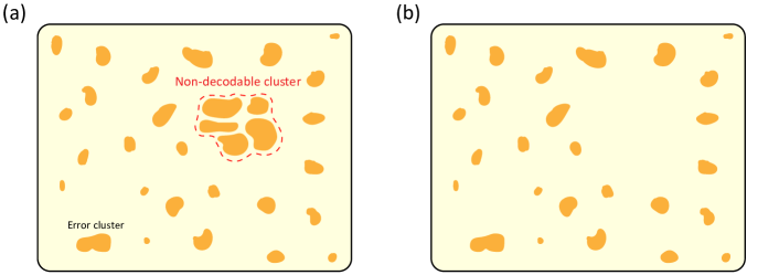
Figure 3: (a) An example of a bottleneck state $\mathbf{x}\in E$ is depicted with the non-decodable cluster highlighted. (b) The partner state $\mathbf{y}(\mathbf{x})\in A$ with this cluster removed. The Gibbs sampler will take a very long time to reach states containing non-decodable clusters at low temperature.

Now that we know that the Gibbs sampler must traverse $E$, we can proceed to bound the hitting time to $E$. Starting in a suitably chosen ensemble of initial decodable states close to codeword $\mathbf{0}$, which are drawn from a set (introduced below) $A$. The idea will be to show tht the transition probability from $A$ to $E$ is exponentially small, which ensures that our Gibbs sampler is unlikely to stray far (in terms of decodability) from the initial codeword state.

We now define our decodable set $A$. Suppose we have a state $\mathbf{x}\in E$. There will, by construction, exist a decodable partner state $\mathbf{y}(\mathbf{x})$ consisting of $\mathbf{x}$ but with the $(s,\ell)$-cluster removed, see Fig. 3. As such, we deduce that $\mathbf{y}(\mathbf{x})$ is a decodable state close to codeword $\mathbf{0}$. We define the set

$$A\equiv\{\mathbf{y}^{\prime}\in\mathbb{F}_{2}^{N}\;:\;\exists\;\mathbf{x}\in E\text{ such that }\mathbf{y}^{\prime}=\mathbf{y}(\mathbf{x})\}.$$ (55)

Notice that all states in $A$ are, by definition, decodable since $\mathbf{x}\in E$ (by definition of $E$) had exactly one dangerous cluster. Let us now upper bound the relative degeneracy $g(E,A)\equiv|E|/|A|$ by estimating the number of possible clusters. For any of the $N$ sites, it can participate in no more than $z^{\gamma m}$ connected subgraphs of size $\gamma m$. There can also be no more than $2^{\gamma m}$ configurations of errors in these subgraphs: each site could have an error or not. As a result, we have $g(E,A)\leq N\times(2z)^{\gamma m}$.

By our definition of $\mathcal{G}_{A}$, any term in $\mathcal{H}(\mathbf{x})$ only couples $x_{i}$ and $x_{j}$ if $i\sim j$ are connected by an edge in $\mathcal{G}_{A}$. Therefore, by construction, we deduce that

$$\mathcal{H}(\mathbf{x})=\mathcal{H}(\mathbf{y}(\mathbf{x}))+\mathcal{H}_{\text{cluster}}\,,$$ (56)

where $\mathcal{H}_{\mathrm{cluster}}$ can be bounded using linear confinement:

$$\mathcal{H}_{\text{cluster}}\geq\frac{2}{3}f\gamma m\,.$$ (57)

We can accordingly bound the equilibrium probability ratio of $E$ and $A$ as

$$\frac{\pi[E]}{\pi[A]} \leq\frac{1}{\pi[A]}\sum_{\mathbf{x}\in E}\pi[\mathbf{x}]\leq\frac{1}{\pi[A]}\sum_{\mathbf{x}\in E}\pi[\mathbf{y}(\mathbf{x})]\,\mathrm{e}^{-\frac{2}{3}\beta f\gamma m}$$

$$\leq g(E,A)\times\mathrm{e}^{-\frac{2}{3}\beta f\gamma m}$$

$$\leq N\times\exp\left[-\gamma m\left(\frac{2}{3}\beta f-\log(2z)\right)\right]\,,$$ (58)

where in the first line we used (56) and (57); in the second line we noted that the sum over all $\mathbf{y}(\mathbf{x})$ can count each element of $A$ at most $g(E,A)$ times, and in the third line we used our bound on $g(E,A)$. We can now bound the transition probability from $A$ to $E$ at any time $t$ in terms of a ratio of their equilibrium probabilities:

$$\mathbf{P}_{t}[A\rightarrow E] \equiv\sum_{\mathbf{y}\in A}\mathbf{P}_{t}[\mathbf{y}\rightarrow E]\frac{\pi[\mathbf{y}]}{\pi[A]}=\sum_{\mathbf{x}\in E}\sum_{\mathbf{y}\in A}\mathbf{P}_{t}[\mathbf{y}\rightarrow\mathbf{x}]\,\frac{\pi[\mathbf{y}]}{\pi[A]}$$

$$=\frac{1}{\pi[A]}\sum_{\mathbf{x}\in E}\sum_{\mathbf{y}\in A}\mathbf{P}_{t}[\mathbf{x}\rightarrow\mathbf{y}]\,\pi[\mathbf{x}]=\frac{1}{\pi[A]}\sum_{\mathbf{x}\in E}\mathbf{P}_{t}[\mathbf{x}\rightarrow A]\,\pi[\mathbf{x}]$$

$$\leq\frac{\pi[E]}{\pi[A]}\leq N\times\exp\left[-\gamma m\left(\frac{2}{3}\beta f-\log(2z)\right)\right]\,.$$ (59)

In the second line we used detailed balance (41) and summed over states in $A$; in the third line we bounded $\mathbf{P}_{t}[\mathbf{x}\rightarrow A]\leq 1$ and used (B.3). Inverting the above transition probability gives us a lower bound on the expected hitting time:

$$t_{\rm hit}[A\rightarrow E]\geq N^{-1}\times\exp\left[\gamma m\left(\frac{2}{3}\beta f-\log(2z)\right)\right]\,.$$ (60)

Thus, the hitting time will be exponentially long in the polynomial system size $m=\Theta\big{(}\sqrt{N}\big{)}$ as long as

$$\beta>\frac{3}{2f}\log(2z)=3\left(1+\frac{1}{\gamma m-1}\right)\log(2z)\,.$$ (61)

Crucially, none of the above steps required counting any (reduced) error clusters of size greater than $\gamma m$, and so we never left the linear confinement regime. By the Markov chain bottleneck theorem, we conclude that (60) is a lower bound on the mixing time if $\beta>\beta_{\mathrm{c}}$ in the thermodynamic limit, wherein $m,n\rightarrow\infty$. ∎

The Peierls argument for the 2D Ising model demonstrates that, below a critical temperature, domain walls are locally unfavorable and hence are globally suppressed. In the same spirit, we have shown that local thermal fluctuations below a certain temperature under the HGP Hamiltonian are unlikely to produce adversarial error clusters which would cause eventual maximum-likelihood decoding to fail. However, unlike the full Peierls argument, which would examine adversarial clusters of all sizes, we only focus on clusters of sizes near the code distance. For local Gibbs sampling, this restriction gives rise to a dynamical bottleneck which prevents ergodicity. Since the dynamics of $X$ and $Z$ errors are equivalent, the thermal Gibbs sampler achieves a thermal/passive quantum memory – encoded quantum information survives for a time which is exponentially long in the (polynomial) system size.

Combining Theorem A.6, Theorem B.4 and Theorem B.8, we obtain the following Corollary.

Corollary B.9 (Typical quantum LDPC memory).

If $\Delta_{C}>\Delta_{B}\geq 7$, then the quantum CSS code produced from the hypergraph product of a classical code chosen uniformly from the $(\Delta_{B},\Delta_{C})$-LDPC ensemble at fixed $n$ has, with probability one (as $n\rightarrow\infty$): (1) a dynamical phase transition corresponding to a non-analyticity in $\log t_{\mathrm{mix}}(\beta)$, the mixing time of the Metropolis Gibbs sampler, as a function of $\beta$; (2) no thermodynamic phase transition (non-analyticity in $\log Z(\beta)$).

Lastly, we note that Theorem B.8 can be straightforwardly adapted to the classical LDPC setting to obtain an alternative bound on the classical critical temperature, as formalized in the following Corollary.

Corollary B.10 (Alternative classical mixing time bound to Theorem A.12).

Let $\mathcal{C}$ be a $(\Delta_{B},\Delta_{C})$-LDPC code of length $n$ whose Tanner graph is a $(\gamma=\Omega(1),\delta<1/2)$ left-expander. Let

$$z\equiv\Delta_{B}\left(\Delta_{C}-1\right)\,.$$ (62)

Then as $n\rightarrow\infty$, there exists a critical inverse temperature

$$\beta_{\rm c}\leq\frac{\log(2z)}{\Delta_{B}(1-2\delta)}$$ (63)

such that for all $\beta>\beta_{\rm c}$, the mixing time of Gibbs sampling is bounded by

$$t_{\rm mix}\geq\mathrm{e}^{\alpha n}$$ (64)

for some constant $\alpha(\beta)>0$ independent of $n$.

Appendix C Numerical simulations

In this appendix, we conduct numerical simulations of passive error correction on both the classical and quantum LDPC codes previously discussed. For the classical codes, we randomly sample from the $(4,5)$-LDPC ensemble using the configuration model: we initialize $n$ bits and $\frac{5}{4}n$ checks and pair up their emanating edges according to a random permutation. For the quantum codes, we randomly sample from the $(7,8)$-HGP ensemble by constructing $(7,8)$-LDPC codes using the configuration model and taking the hypergraph product to produce $(8,15)$-LDPC quantum CSS codes. Since the $X$ and $Z$ sectors of the HGP are identical, we focus only on decoding of $X$ errors. All of our sampled codes have no check redundancies. In both classical and quantum simulations, we begin in the $\mathbf{0}$ codeword. We then simulate thermal equilibration at a chosen temperature by performing $\Delta t=100$ Monte Carlo sweeps of the Metropolis algorithm, where each sweep updates all sites exactly once. After the Monte Carlo sweeps, we feed the error syndrome into a belief-propagation decoder Kschischang et al. (2001) and verify if the output codeword is $\mathbf{0}$. For HGP codes, the presence of small loops in their Tanner graphs prevents the convergence of belief propagation (BP), and so we also perform ordered-statistics post-processing Panteleev and Kalachev (2021). We use open source software to implement belief propagation Roffe (2022) and ordered-statistics decoding (BP+OSD) Roffe et al. (2020). In particular, we perform a maximum of 10 iterations of minimum-sum BP with the additional use of OSD-0 for quantum decoding. We sweep from low to high temperatures and terminate the simulation if we fail to decode all Monte Carlo samples at a given temperature. For comparison, we also simulate thermal equilibration for the 2D surface code with minimum-weight perfect-matching (MWPM) decoding, using the open-source software PyMatching Higgott and Gidney (2023).

The simulation results are showcased in Fig. 4. We observe evidence of dynamical transitions for both classical and quantum LDPC codes from (i) the suppression of logical errors with increasing system size and (ii) the asymptotic behavior of the logical error rate with increasing equilibration time. For the classical $(4,5)$-LDPC ensemble, we observe this transition near $T_{\mathrm{c}}=1/\beta_{\mathrm{c}}\approx 1.2$, consistent with our lower bounds of $T_{\rm c}\geq 0.17$ from Theorem A.12 and $T_{\rm c}\geq 0.38$ from Corollary B.10. For the quantum $(7,8)$-HGP ensemble, we observe a transition around $T\approx 1.1$, consistent with our lower bound of $T_{\rm c}\geq 0.063$ from Theorem B.8. In contrast, for the 2D surface code, we observe that the logical error probability is independent of system size. Indeed we should expect such behavior since at any nonzero temperature there is a finite density of anyons, which can diffuse freely to form an extensive error string in constant time Brown et al. (2016).

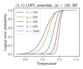
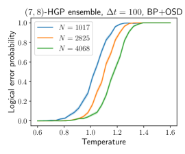
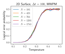
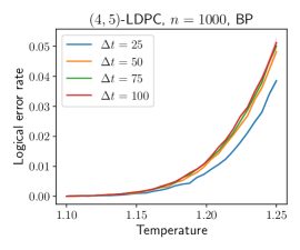
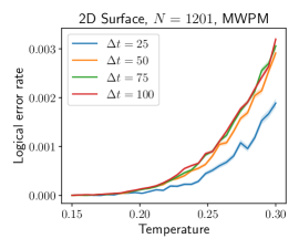
Figure 4: Top: The logical block error probability as a function of temperature is plotted. We set $\Delta t=100$ and sample several codes from the $(4,5)$-LDPC ensemble, $(7,8)$-HGP ensemble and 2D surface code family. Bottom: The logical block error rate (normalized by $\Delta t$) as a function of temperature is plotted near the observed transition point. We examine one particular code from each of the aforementioned ensembles and vary the equilibration time. Error bands (shaded) denote the standard error.

Appendix D Open quantum system dynamics

This appendix contains details of our discussion of MFQEC and passive error correction.

D.1 Lindblad dynamics

Our goal is to prepare a stationary Gibbs state

$$\sigma\propto\mathrm{e}^{-\beta\mathcal{H}},$$ (65)

where

$$\mathcal{H}=-\sum_{\text{stabilizer }a}S_{a}$$ (66)

and as in the main text, the stabilizers $\{S_{a}\}$ are a set of mutually commuting Pauli strings, i.e., $S_{a}^{2}=\mathds{1}$ and $[S_{a},S_{b}]=0$ for all $a$, $b$. In this appendix, we assume that each $S_{a}$ is independent (in the sense that one cannot be built out of a product of any others), as was the case for the non-redundant codes described above. The Gibbs state is diagonal in a basis that consists of eigenvectors of all Pauli strings $\{S_{a}\}$, which we can denote as $\sigma=\sum_{s}\sigma_{s}|s\rangle\langle s|$. Notice that with this choice, there remain $2^{K}$ possible $s$ for each set of stabilizer eigenvalues, and we will be a little lazy and omit that explicit notation.

Let’s start with ideal circuits without any errors. We choose a Lindbladian of Davies form Davies (1979):

$$\partial_{t}\rho=\mathcal{L}(\rho)=\sum_{ss^{\prime}}L_{ss^{\prime}}\left(|s\rangle\langle s^{\prime}|\rho|s^{\prime}\rangle\langle s|-\frac{1}{2}\{|s^{\prime}\rangle\langle s^{\prime}|,\rho\}\right)\,,$$ (67)

where the coefficients $L_{ss^{\prime}}$ are positive and satisfy $L_{ss^{\prime}}=\mathrm{e}^{-\beta\left(\mathcal{H}_{s}-\mathcal{H}_{s^{\prime}}\right)}L_{s^{\prime}s}$. We also want the dynamics to be local, which means all the jump operators only act on finite numbers of qubits. Consider an operator $P$, which can be a Pauli operator on a single qubit or a Pauli string on multiple qubits. If there exists some stabilizers that anticommute with $P$: $\mathcal{A}_{P}\equiv\{a\,|\,S_{a}P+PS_{a}=0\}$ and $\mathcal{A}_{P}\neq\emptyset$, we can choose jump operators that consist of $P$ and projections:

$$P(\mathbf{n})=P\Pi_{P}(\mathbf{n})\equiv P\left[\prod_{a\in\mathcal{A}_{P}}\frac{1}{2}(I+n_{a}S_{a})\right]\,,$$ (68)

where $\mathbf{n}\equiv\{n_{a}\}_{a\in\mathcal{A}_{P}}$ and $n_{a}\in\{-1,+1\}$, which defines the projector $\Pi_{P}(\mathbf{n})$. Note that $P=\sum_{\mathbf{n}}P(\mathbf{n})$. Since we have an LDPC CSS code, any local operator $P$ is only involved in a finite number of stabilizers, and each stabilizer has support on a finite number of Pauli operators, so the jump operator $P(\mathbf{n})$ is also $\mathsf{k}$-local. A $\mathsf{k}$-local Lindbladian with stationary state $\sigma$ can then be found explicitly Guo et al. (to appear):

$$\mathcal{L}(\rho)=\sum_{P,\mathbf{n}}\gamma_{P(\mathbf{n})}\mathcal{L}_{P(\mathbf{n})}(\rho)=\sum_{P,\mathbf{n}}\gamma_{P(\mathbf{n})}\left(P(\mathbf{n})\rho P(\mathbf{n})^{\dagger}-\frac{1}{2}\{\Pi_{P}(\mathbf{n}),\rho\}\right)\,,$$ (69)

with

$$\gamma_{P(\mathbf{n})}=\mathrm{e}^{-2\beta\sum_{a\in\mathcal{A}_{P}}n_{a}}\gamma_{P(\mathbf{-n})}$$ (70)

correspoding to “Gibbs sampling” dynamics that protects the Gibbs mixed state.

We now show that the dynamics above can be effectively implemented using ancilla qubits and quantum gates. If we want to implement the dynamics $\mathcal{L}_{P(\mathbf{n})}$, we need an ancilla qubit that is initialied as $\ket{0}$ for each $a\in\mathcal{A}_{P}$. The ancilla qubits can store information about the physical qubits, which can then be used to apply feedback. For each stabilizer $S_{a}=\prod_{i}P_{i}$ that anticommutes with $P$, where $P_{i}$ is a Pauli operator on qubit $i$, we apply gates $\prod_{i}\mathrm{e}^{\mathrm{i}\frac{\pi}{4}(I_{i}-P_{i})(I_{a}-X_{a})}$ to extract syndromes, where $I_{a}$ and $X_{a}$ are operators on the ancilla qubits for $S_{a}$. After applying gates for each stabilizers, we apply gate

$$U_{\mathrm{feedback}}=\exp\left[\mathrm{i}\frac{\pi}{2}(I-P)\prod_{a}\frac{I_{a}+n_{a}Z_{a}}{2}\right]$$ (71)

as the feedback. The last step is to reset all ancilla qubits to $\ket{0}$.

Neglecting the time it takes to apply the gates above, the dynamics we implemented in the previous paragraph on physical and ancilla qubits can be converted into an effective Lindbladian acting only on the original physical qubits. After tracing out ancilla qubits, we find that

$$\mathcal{L}_{P(\mathbf{n})}^{\prime}(\rho)=P(\mathbf{n})\rho P(\mathbf{n})^{\dagger}-\frac{1}{2}\{\Pi_{P}(\mathbf{n}),\rho\}+\sum_{\mathbf{m}\neq\mathbf{n}}\Pi_{P}(\mathbf{m})\rho\Pi_{P}(\mathbf{m})-\frac{1}{2}\{\Pi_{P}(\mathbf{m}),\rho\}\,.$$ (72)

Since the projector $\Pi_{P}(\mathbf{m})$ commutes with $\sigma$, the additional dynamics we implemented other than $\mathcal{L}_{P(\mathbf{n})}$ will not affect the stationarity of $\sigma$, so we can effectively implement $\mathcal{L}_{P(\mathbf{n})}$ with the above process.

Ultimately, using this Lindbladian picture, we can predict the rates at which we should correct for errors in the MFQEC circuit; the only difference in this mathematical framework is that we apply this feedback effectively instantaneously and at a continuous rate for each qubit.

For the whole dynamics $\mathcal{L}$ in (69), instead of implementing only $\mathcal{L}_{P(\mathbf{n})}$ at a time, we can implement $\sum_{\mathbf{n}}\gamma_{P(\mathbf{n})}\mathcal{L}_{P(\mathbf{n})}$ together: for each operator $P$, in time interval $\text{d}t$, we apply gates that extract syndromes with probability

$$p_{\text{syndrome}}\propto\text{d}t\,\max_{\{\mathbf{m}\}}\left(\gamma_{P(\mathbf{m})}\right),$$ (73)

then apply $U_{\mathrm{feedback}}$ for $P(\mathbf{n})$ with probability

$$p_{P(\mathbf{n})}=\frac{\gamma_{P(\mathbf{n})}}{\max_{\{\mathbf{m}\}}\left(\gamma_{P(\mathbf{m})}\right)}.$$ (74)

The Lindbladian thus becomes

$$\mathcal{L}^{\prime}(\rho) =\sum_{P}\max_{\{\mathbf{m}\}}\left(\gamma_{P(\mathbf{m})}\right)\sum_{\mathbf{n}}\mathcal{L}^{\mathrm{ideal}}_{P(\mathbf{n})}(\rho)$$

$$=\sum_{P}\max_{\{\mathbf{m}\}}\left(\gamma_{P(\mathbf{m})}\right)\sum_{\mathbf{n}}\left(p_{P(\mathbf{n})}P(\mathbf{n})\rho P(\mathbf{n})^{\dagger}+\left(1-p_{P(\mathbf{n})}\right)\Pi_{P}(\mathbf{n})\rho\Pi_{P}(\mathbf{n})-\frac{1}{2}\{\Pi_{P}(\mathbf{n}),\rho\}\right)\,,$$ (75)

which is similar to $\mathcal{L}$ in (69), differing only in terms that don’t affect the stationarity of $\sigma$.

Fig. 5 shows two examples of such dynamics. There are three stabilizers: $S_{1}=Z_{1}Z_{2}Z_{3}Z_{4}$, $S_{2}=Z_{3}Z_{4}$ and $S_{3}=Z_{4}Z_{5}$. In the first example, consider Pauli operator $X_{3}$ that act on $q_{3}$, there are two stabilizers that anticommute with $X_{3}$, so jump operators related to $X_{3}$ would be $X_{3}(n_{1},n_{2})=\frac{1}{4}X_{3}(I+n_{1}S_{1})(I+n_{2}S_{2})$. The first dashed box in Fig. 5 together with gates applied on $a_{1}$ and $a_{2}$ show how to implement $\mathcal{L}_{X_{3}(-1,-1)}$. Similarly, the second box and all other gates outside the boxes show how to implement $\mathcal{L}_{X_{4}(1,-1,-1)}$. The channel $R$ resets the ancilla qubits to $\ket{0}$, and is implemented as follows:

$$R_{i}[\rho]=\mathrm{tr}_{i}\rho\otimes|0\rangle\langle 0|_{i}.$$ (76)

[row sep=0.7cm,between origins] $\ket{q_{1}}$ & 5
$\ket{q_{2}}$ 4
$\ket{q_{3}}$ 4 [6,steps=1,style=dashed,rounded corners, inner sep=2pt,background,label style=label position=below,anchor=north,yshift=-0.2cm]$X_{3}$
$\ket{q_{4}}$ 4 [5,steps=2,style=dashed,rounded corners, inner sep=2pt,background,label style=label position=below,anchor=north,yshift=-0.2cm]$X_{4}$
$\ket{q_{5}}$ 3
$\ket{a_{1}}=|{0}\rangle$ -3 X -2 R
$\ket{a_{2}}=|{0}\rangle$ -1 -1 R
$\ket{a_{3}}=|{0}\rangle$ -1 R

Figure 5: Two examples of how to implement dynamics in (69). There are three stabilizers: $S_{1}=Z_{1}Z_{2}Z_{3}Z_{4}$, $S_{2}=Z_{3}Z_{4}$ and $S_{3}=Z_{4}Z_{5}$ so we need three ancilla qubits to extract syndromes by the CNOT gates outside the dashed boxes. The gates in the boxes apply $X_{3}$ and $X_{4}$ according to different syndromes. The reset channel $R$ forces ancilla qubits to their initial state $\ket{0}$.

D.2 Fault tolerance

Now let us relate the Gibbs sampling dynamics above to quantum error correction. For simplicity, we focus on correcting for single-qubit Pauli errors, with generic correction strategies described in Guo et al. (to appear). If $Q$ is a Pauli string acting on O(1) sites, then adding such an error modifies our Lindbladian to:

$$\mathcal{L}(\rho)\to\mathcal{L}(\rho)+g\left(Q\,\rho\,Q-\rho\right)\,,$$ (77)

where $g>0$ is the rate of the Pauli error, and $Q$ is a single-qubit Pauli that doesn’t commute with some of the stabilizers. Since $Q=\sum_{\mathbf{n}}Q(\mathbf{n})$, we have

$$g\left(Q\,\rho\,Q-\rho\right)=g\sum_{\mathbf{m},\mathbf{n}}\left(Q(\mathbf{m})\,\rho\,Q(\mathbf{n})^{\dagger}-\frac{1}{2}\{Q(\mathbf{n})^{\dagger}Q(\mathbf{m}),\rho\}\right)\,.$$ (78)

Because

$$Q(\mathbf{m})\,\sigma\,Q(\mathbf{n})^{\dagger}-\frac{1}{2}\{Q(\mathbf{n})^{\dagger}Q(\mathbf{m}),\sigma\}=\delta_{\mathbf{m}\mathbf{n}}\left(Q\Pi_{Q}(\mathbf{n})\,\sigma\,\Pi_{Q}(\mathbf{n})Q-\frac{1}{2}\{\Pi_{Q}(\mathbf{n}),\sigma\}\right),$$ (79)

when $\mathbf{m}\neq\mathbf{n}$, this part of error doesn’t affect stationarity and doesn’t need to be corrected. For the remaining terms that do have $\mathbf{m}=\mathbf{n}$, this part is in the same form as (69) with different coefficients. We can just increase these coefficients until the ratios between the coefficients are also the same as (69) so the stationarity of $\sigma$ still holds and the error is effectively corrected. As an example, one way to correct the error in (77) is to increase the coefficient $\gamma_{Q(\mathbf{n})}$ by

$$\delta\gamma_{Q(\mathbf{n})}=\text{sgn}\left(-\sum n\right)\left(\mathrm{e}^{-2\beta\sum n}-1\right)g\,.$$ (80)

So far, we assumed all the gates we apply are perfect. We will now assume that the system is subject to incoherent Pauli errors for each possible qubit (physical and ancilla). For all the CNOT-like gates, the corresponding errors are equivalent to applying random Pauli strings on both sides of the gates. For the reset operations, the errors would lead to the wrong initial states of the ancilla qubits, which is also equivalent to applying Pauli gates to the correct initial states. We can move all the Pauli errors to the right-hand side of these gates and then implement a modified dynamics. For example, suppose we wish to implement the process $\mathcal{L}_{P(\mathbf{n})}$ described above, which in general contained unitary operations corresponding to gates of the form $\prod_{i}\mathrm{e}^{\mathrm{i}\frac{\pi}{4}(I_{i}-P_{i})(I_{a}-X_{a})}$. These gates become

$$\prod_{i}\mathrm{e}^{\mathrm{i}\frac{\pi}{4}(I_{i}-P_{i})(I_{a}-X_{a})}\rightarrow\prod_{i}Z_{\mathrm{error}}\mathrm{e}^{\mathrm{i}\frac{\pi}{4}(I_{i}-P_{i})(I_{a}-X_{a})}Z_{\mathrm{error}}=\prod_{i}\mathrm{e}^{\mathrm{i}\frac{\pi}{4}(I_{i}\pm P_{i})(I_{a}\pm X_{a})},$$ (81)

where the $\pm$ signs at the end correspond to whether or not the error commuted or anticommuted with the $P_{i}$ or $X_{a}$. We can handle other errors analogously: $\mathrm{e}^{\mathrm{i}\frac{\pi}{2}(I-P)\prod_{a}\frac{1}{2}(I_{a}+n_{a}Z_{a})}\rightarrow\mathrm{e}^{\mathrm{i}\frac{\pi}{2}(I\pm P)\prod_{a}\frac{1}{2}(I_{a}\pm n_{a}Z_{a})}$ after moving all the Pauli errors to the right, which is equivalent to implementing $\mathcal{L}_{P(\mathbf{n}^{\prime})}$ with $\mathbf{n}^{\prime}\neq\mathbf{n}$ and then applying the Pauli errors. Recall that $\mathcal{L}_{P(\mathbf{n})}$ was defined in (69). Putting all of this together, we find that our Lindbladian $\mathcal{L}_{P(\mathbf{n})}$ is modified to

$$\mathcal{L}_{P(\mathbf{n})}(\rho) \rightarrow\sum_{Q_{e},\mathbf{n}^{\prime}}p(Q_{e},\mathbf{n}^{\prime}|P(\mathbf{n}))\left(Q_{e}P(\mathbf{n}^{\prime})\rho P(\mathbf{n}^{\prime})^{\dagger}Q_{e}-\frac{1}{2}\{\Pi_{P}(\mathbf{n}^{\prime}),\rho\}\right)$$

$$\rightarrow\mathcal{L}_{P(\mathbf{n})}^{\mathrm{ideal}}(\rho)+\sum_{Q_{e},\mathbf{m}}\delta p_{Q_{e}P(\mathbf{m}),P(\mathbf{n})}\mathcal{L}_{Q_{e}P(\mathbf{m})}(\rho),$$ (82)

where in the first line, $Q_{e}$ are the Pauli operations (including $I$, or having no error) that have been moved to the right and $p(Q_{e},\mathbf{n}^{\prime}|P(\mathbf{n}))$ is the probability of having Pauli “error” $Q_{e}$ and applying $P(\mathbf{n}^{\prime})$ when the “apparent” syndrome measurements returned $\mathbf{n}$. In the second line, we rewrite the expression to emphasize that when $p(Q_{e},\mathbf{n}^{\prime}|P(\mathbf{n}))$ is small (i.e. the gates are high fidelity), the Lindbladian is quite close to the “ideal case”. As the ancilla qubit feedback only corrects for single qubit errors, we emphasize that $Q_{e}$ will contain only single qubit terms once we trace out the state of the ancilla qubits (as is appropriate, once they are reset during MFQEC).

In the presence of errors throughout our circuit, it is useful to expand the sum over $\mathbf{n}$ above to incorporate all of the $X$ or $Z$ type stabilizers that act on a given site (not just the ones that anticommute with Pauli $P$). After all, the error $Q_{e}$ may be a $Z$ type error if we intended to correct an $X$ type error. So the most generic type of Lindbladian modeling our MFQEC protocol takes the form of

$$\mathcal{L}=\sum_{P,\mathbf{n}}\gamma_{P(\mathbf{n})}\mathcal{L}^{\mathrm{ideal+error}}_{P(\mathbf{n})}+\sum_{P,\mathbf{n}}\delta\gamma_{Q_{e}P(\mathbf{n})}\mathcal{L}_{Q_{e}P(\mathbf{n})}(\rho)$$ (83)

where $\mathcal{L}^{\mathrm{ideal+error}}_{P(\mathbf{n})}$ includes the physical qubit errors discussed in (77), and

$$\delta\gamma_{Q_{e}P(\mathbf{n})}=\sum_{Q^{\prime}P(\mathbf{n}^{\prime})}\delta p_{Q_{e}P(\mathbf{m}),Q^{\prime}(\mathbf{n^{\prime}})}\cdot\gamma_{Q^{\prime}(\mathbf{n}^{\prime})}.$$ (84)

We will consider an ideal protocol where we apply $Y$ errors deliberately at some rate, to ensure that all $\gamma_{P(\mathbf{n})}>0$, which will shortly prove convenient. Our goal is to show that $\mathcal{L}$ is an exact Gibbs sampler, which will be satisfied so long as the detailed balance condition Guo et al. (to appear)

$$(\gamma+\delta\gamma)_{P(\mathbf{n}_{\mathrm{acomm}},\mathbf{n}_{\mathrm{comm}})}=(\gamma+\delta\gamma)_{P(-\mathbf{n}_{\mathrm{acomm}},\mathbf{n}_{\mathrm{comm}})}\mathrm{e}^{-2\beta\sum_{\text{acomm }a}n_{a}}.$$ (85)

Here $\mathbf{n}_{\mathrm{acomm/comm}}$ denote the stabilizer values of the anticommuting/commuting stabilizers that act on the same site as single-qubit Pauli $P$. (85) is clearly solved if

$$(\gamma+\delta\gamma)_{P(\mathbf{n}_{\mathrm{acomm}},\mathbf{n}_{\mathrm{comm}})}=\gamma_{0}\times\max\left(1,\mathrm{e}^{-2\beta\sum_{\text{acomm }a}n_{a}}\right)=\gamma^{\mathrm{Gibbs}}_{P(\mathbf{n}_{\mathrm{acomm}},\mathbf{n}_{\mathrm{comm}})}$$ (86)

where $\gamma_{0}>0$ is some fixed positive constant. Since $\gamma^{\mathrm{Gibbs}}$ is positive, we deduce that there exists a finite, $N$-independent value of $\gamma_{0}$ such that for sufficiently small error rate $\delta p$, (86) admits a solution for which all of the rates $\gamma_{P(\mathbf{n})}>0$, because for sufficiently small $\delta p$, the matrix $(I+\delta p)^{-1}$ is invertible and has bounded matrix elements.

D.3 Sort channel implementation

The Gibbs sampler that we described in the main text requires a non-unitary $\mathsf{SORT}$ channel to work. Here we provide an explicit implementation for this channel. It can be efficiently realized with sorting networks Knuth (1997); Bundala and Závodný (2013); Codish et al. (2014); Harder (2022), which are circuits constructed using a 2-input binary comparator as a primitive: see Fig. 6 for a circuit depiction and Table 1 for an optimal gate-cost analysis. The use of native Toffoli (CCNOT) gates in Rydberg systems Shi (2018); Yin et al. (2020) would allow one to bypass the two-qubit gate decomposition and significantly reduce the overhead.

[column sep=0.3em] & [1em][open]1 [1em][open]2 [1em] [1em][open]4 [1em][1em][1em]
[open]0 [open]2 [open]1 [open]4 [open]1
[open]1 [open]0 [open]0 [open]4 [open]2 [open]0
[open]0 [open]0 [open]4 [open]2 [open]1
[open]1 [open]2 [open]0 [open]0 [open]0
[open]0 [open]2 [open]1 [open]0 [open]0 [open]1
[open]1[2,steps=1,style=dashed,rounded corners,fill=blue!10, inner xsep=2pt,background,label style=label position=below,anchor=north,yshift=-0.2cm]Comparator [open]0 [open]0 [open]0 [open]0
[open]0 [open]0 [open]0                   $a$ & 2 1 $\min(a,b)$
$b$ 1 $\max(a,b)$
$\ket{0}$ 0 R

Figure 6: Left: An optimal sorting network for 8 inputs is depicted using 19 comparators with a circuit depth of 6 Batcher (1968). Right: The 2-input comparator gadget (boxed in the left circuit) is shown, which sorts the binary inputs $a,b$ using an ancilla, a CNOT gate and a Fredkin (CSWAP) gate. The Fredkin gate can be decomposed into 7 CNOT gates and single-qubit rotations M. Q. Cruz and Murta (2024).

$n_{\rm in}$	3	4	5	6	7	8	9	10	11	12
Depth	3	3	5	5	6	6	7	7	8	8
Size	3	5	9	12	16	19	25	29	35	39
2-qubit gates	24	40	72	96	128	152	200	232	280	312

Table 1: The depth and size (number of comparators) of optimal sorting networks for a range of inputs is tabulated. The number of 2-qubit gates ($8\times$ size) upon gate decomposition is also shown.

As a concrete example, let us now compare passive vs. active quantum error correction for the smallest (guaranteed) self-correcting HGP code, again focusing on the case for $X$ errors as the $Z$ error discussion is analogous. To keep the discussion a little bit simpler, we focus on just a simple-majority “greedy decoder”, which we expect will perform at least as well as the Gibbs sampler (which sometimes introduces errors). We draw a random classical code from the regular $(7,8)$-LDPC ensemble which exhibits $\delta<1/6$ expansion with high probability (Theorem A.6). We then take the hypergraph product of this classical code with itself to obtain a $(8,15)$-LDPC quantum CSS code. Since the check weight is 15, the syndrome extraction circuit to couple measure/ancilla qubits with physical qubits via two-qubit gates has depth at least 15. At this point, the procedures for active and passive error correction differ. For active error correction, we would now simply measure all ancilla qubits in the computational basis and feed the results into a classical decoding algorithm. The output of this decoding algorithm then allows us to undo the error or alternatively track the Pauli frame of the code in software. For passive error correction, we essentially need to run the decoding algorithm as a quantum circuit itself. Since each physical qubit participates in no more than 8 checks, according to Table 1, we need to run a depth-6 sorting network on 8 ancilla qubits per physical qubit. Each comparator contains a Fredkin gate (Fig. 6), which can be further decomposed into 2 CNOTs and a Toffoli. With the ability to perform native Toffoli gates, our ancilla sorting circuit will thus have depth 24; we note that further parallelization may reduce this depth. After sorting, we then apply a CNOT gate between the 4th ancilla qubit from the right (control) and the physical qubit (target), which implements the majority vote. The total circuit depth for passive decoding after syndrome extraction is hence 25, assuming native Toffoli gates. Using a direct majority-vote circuit, rather than sorting, may further reduce the gate cost Kheirandish et al. (2020); e.g. a 5-input majority voter would use 50 2-qubit gates instead of 72 for the sorting network.

For disconnected physical qubits that do not share any checks, we run simultaneous decoding in parallel. To run this entire decoding step in one round, we can introduce 14 additional ancilla qubits per syndrome qubit to which we copy the syndrome values via CNOT gates, thus enabling simultaneous decoding on all physical qubits. The copying of each measurement outcome to many different ancillas will add at most circuit depth 14.

We note that additional overhead will be required if we wanted to implement the full Gibbs sampler.

References

- Thomas (1989) Lawrence E. Thomas, “Bound on the mass gap for finite volume stochastic ising models at low temperature,” Communications in Mathematical Physics 126, 1–11 (1989).
- Dennis et al. (2002) Eric Dennis, Alexei Kitaev, Andrew Landahl, and John Preskill, “Topological quantum memory,” Journal of Mathematical Physics 43, 4452–4505 (2002).
- Onsager (1944) Lars Onsager, “Crystal statistics. i. a two-dimensional model with an order-disorder transition,” Phys. Rev. 65, 117–149 (1944).
- Alicki et al. (2008) R. Alicki, M. Horodecki, P. Horodecki, and R. Horodecki, “On thermal stability of topological qubit in kitaev’s 4d model,” (2008), arXiv:0811.0033 [quant-ph] .
- Yoshida (2011) Beni Yoshida, “Feasibility of self-correcting quantum memory and thermal stability of topological order,” Annals of Physics 326, 2566–2633 (2011).
- Hastings (2011) Matthew B. Hastings, “Topological order at nonzero temperature,” Physical Review Letters 107 (2011), 10.1103/physrevlett.107.210501.
- Brown et al. (2016) Benjamin J. Brown, Daniel Loss, Jiannis K. Pachos, Chris N. Self, and James R. Wootton, “Quantum memories at finite temperature,” Reviews of Modern Physics 88 (2016), 10.1103/revmodphys.88.045005.
- Liu and Lieu (2024) Yu-Jie Liu and Simon Lieu, “Dissipative phase transitions and passive error correction,” Phys. Rev. A 109, 022422 (2024).
- Xu et al. (2023) Qian Xu, J. Pablo Bonilla Ataides, Christopher A. Pattison, Nithin Raveendran, Dolev Bluvstein, Jonathan Wurtz, Bane Vasic, Mikhail D. Lukin, Liang Jiang, and Hengyun Zhou, “Constant-overhead fault-tolerant quantum computation with reconfigurable atom arrays,” (2023), arXiv:2308.08648 [quant-ph] .
- Hong et al. (2023) Yifan Hong, Matteo Marinelli, Adam M. Kaufman, and Andrew Lucas, “Long-range-enhanced surface codes,” (2023), arXiv:2309.11719 [quant-ph] .
- Gallager (1962) R. Gallager, “Low-density parity-check codes,” IRE Transactions on Information Theory 8, 21–28 (1962).
- Breuckmann and Eberhardt (2021) Nikolas P. Breuckmann and Jens Niklas Eberhardt, “Quantum low-density parity-check codes,” PRX Quantum 2 (2021), 10.1103/prxquantum.2.040101.
- Bravyi et al. (2010) Sergey Bravyi, David Poulin, and Barbara Terhal, “Tradeoffs for reliable quantum information storage in 2d systems,” Physical Review Letters 104 (2010), 10.1103/physrevlett.104.050503.
- Metropolis et al. (1953) Nicholas Metropolis, Arianna W. Rosenbluth, Marshall N. Rosenbluth, Augusta H. Teller, and Edward Teller, “Equation of State Calculations by Fast Computing Machines,” The Journal of Chemical Physics 21, 1087–1092 (1953), https://pubs.aip.org/aip/jcp/article-pdf/21/6/1087/18802390/1087_1_online.pdf .
- Hastings (1970) W. K. Hastings, “Monte Carlo sampling methods using Markov chains and their applications,” Biometrika 57, 97–109 (1970), https://academic.oup.com/biomet/article-pdf/57/1/97/23940249/57-1-97.pdf .
- Sipser and Spielman (1996) M. Sipser and D.A. Spielman, “Expander codes,” IEEE Transactions on Information Theory 42, 1710–1722 (1996).
- Richardson and Urbanke (2008) Tom Richardson and Ruediger Urbanke, Modern coding theory (Cambridge University Press, 2008).
- Freedman and Hastings (2013) M. H. Freedman and M. B. Hastings, “Quantum systems on non--hyperfinite complexes: A generalization of classical statistical mechanics on expander graphs,” (2013), arXiv:1301.1363 [quant-ph] .
- Weinstein et al. (2019) Zack Weinstein, Gerardo Ortiz, and Zohar Nussinov, “Universality classes of stabilizer code hamiltonians,” Physical Review Letters 123 (2019), 10.1103/physrevlett.123.230503.
- Rakovszky and Khemani (2023) Tibor Rakovszky and Vedika Khemani, “The Physics of (good) LDPC Codes I. Gauging and dualities,” (2023), arXiv:2310.16032 [quant-ph] .
- Rakovszky and Khemani (2024) Tibor Rakovszky and Vedika Khemani, “The Physics of (good) LDPC Codes II. Product constructions,” (2024), arXiv:2402.16831 [quant-ph] .
- Ben-Sasson et al. (2009) Eli Ben-Sasson, Venkatesan Guruswami, Tali Kaufman, Madhu Sudan, and Michael Viderman, “Locally testable codes require redundant testers,” in 2009 24th Annual IEEE Conference on Computational Complexity (2009) pp. 52–61.
- Panteleev and Kalachev (2022) Pavel Panteleev and Gleb Kalachev, “Asymptotically good quantum and locally testable classical ldpc codes,” in Proceedings of the 54th Annual ACM SIGACT Symposium on Theory of Computing, STOC 2022 (Association for Computing Machinery, New York, NY, USA, 2022) p. 375–388.
- Lin and Hsieh (2022) Ting-Chun Lin and Min-Hsiu Hsieh, “-locally testable codes from lossless expanders,” (2022), arXiv:2201.11369 [cs.IT] .
- Dinur et al. (2022a) Irit Dinur, Shai Evra, Ron Livne, Alexander Lubotzky, and Shahar Mozes, “Good locally testable codes,” (2022a), arXiv:2207.11929 [cs.IT] .
- Calderbank and Shor (1996) A. R. Calderbank and Peter W. Shor, “Good quantum error-correcting codes exist,” Physical Review A 54, 1098–1105 (1996).
- Steane (1996) Andrew Steane, “Multiple-particle interference and quantum error correction,” Proceedings of the Royal Society of London. Series A: Mathematical, Physical and Engineering Sciences 452, 2551–2577 (1996).
- Leverrier and Zémor (2022) Anthony Leverrier and Gilles Zémor, “Quantum tanner codes,” (2022), arXiv:2202.13641 [quant-ph] .
- Dinur et al. (2022b) Irit Dinur, Min-Hsiu Hsieh, Ting-Chun Lin, and Thomas Vidick, “Good quantum ldpc codes with linear time decoders,” (2022b), arXiv:2206.07750 [quant-ph] .
- Tillich and Zemor (2014) Jean-Pierre Tillich and Gilles Zemor, “Quantum LDPC codes with positive rate and minimum distance proportional to the square root of the blocklength,” IEEE Transactions on Information Theory 60, 1193–1202 (2014).
- Leverrier et al. (2015) Anthony Leverrier, Jean-Pierre Tillich, and Gilles Zémor, “Quantum expander codes,” in 2015 IEEE 56th Annual Symposium on Foundations of Computer Science (IEEE, 2015).
- Peierls (1936) R. Peierls, “On ising’s model of ferromagnetism,” Mathematical Proceedings of the Cambridge Philosophical Society 32, 477–481 (1936).
- Hastings et al. (2014) Matthew B. Hastings, Grant H. Watson, and Roger G. Melko, “Self-correcting quantum memories beyond the percolation threshold,” Phys. Rev. Lett. 112, 070501 (2014).
- Haah (2011) Jeongwan Haah, “Local stabilizer codes in three dimensions without string logical operators,” Phys. Rev. A 83, 042330 (2011).
- Michnicki (2014) Kamil P. Michnicki, “3d topological quantum memory with a power-law energy barrier,” Phys. Rev. Lett. 113, 130501 (2014).
- Bravyi and Haah (2013) Sergey Bravyi and Jeongwan Haah, “Quantum self-correction in the 3d cubic code model,” Phys. Rev. Lett. 111, 200501 (2013).
- Siva and Yoshida (2017) Karthik Siva and Beni Yoshida, “Topological order and memory time in marginally-self-correcting quantum memory,” Physical Review A 95 (2017), 10.1103/physreva.95.032324.
- Bombin (2015) Héctor Bombin, “Single-shot fault-tolerant quantum error correction,” Physical Review X 5 (2015), 10.1103/physrevx.5.031043.
- Campbell (2019) Earl T Campbell, “A theory of single-shot error correction for adversarial noise,” Quantum Science and Technology 4, 025006 (2019).
- Quintavalle et al. (2021) Armanda O. Quintavalle, Michael Vasmer, Joschka Roffe, and Earl T. Campbell, “Single-shot error correction of three-dimensional homological product codes,” PRX Quantum 2, 020340 (2021).
- Fawzi et al. (2018) Omar Fawzi, Antoine Grospellier, and Anthony Leverrier, “Constant overhead quantum fault-tolerance with quantum expander codes,” in 2018 IEEE 59th Annual Symposium on Foundations of Computer Science (FOCS) (IEEE, 2018).
- Gu et al. (2023) Shouzhen Gu, Eugene Tang, Libor Caha, Shin Ho Choe, Zhiyang He, and Aleksander Kubica, “Single-shot decoding of good quantum LDPC codes,” (2023), arXiv:2306.12470 [quant-ph] .
- Ahn et al. (2002) Charlene Ahn, Andrew C. Doherty, and Andrew J. Landahl, “Continuous quantum error correction via quantum feedback control,” Phys. Rev. A 65, 042301 (2002).
- Sarovar and Milburn (2005) Mohan Sarovar and G. J. Milburn, “Continuous quantum error correction by cooling,” Phys. Rev. A 72, 012306 (2005).
- Stinespring (1955) W. Forrest Stinespring, “Positive functions on c*-algebras,” Proceedings of the American Mathematical Society 6, 211–216 (1955).
- Friedman et al. (2022) Aaron J. Friedman, Chao Yin, Yifan Hong, and Andrew Lucas, “Locality and error correction in quantum dynamics with measurement,” (2022), arXiv:2206.09929 [quant-ph] .
- Sala et al. (2020) Pablo Sala, Tibor Rakovszky, Ruben Verresen, Michael Knap, and Frank Pollmann, “Ergodicity breaking arising from hilbert space fragmentation in dipole-conserving hamiltonians,” Phys. Rev. X 10, 011047 (2020).
- Khemani et al. (2020) Vedika Khemani, Michael Hermele, and Rahul Nandkishore, “Localization from hilbert space shattering: From theory to physical realizations,” Phys. Rev. B 101, 174204 (2020).
- Hart and Nandkishore (2022) Oliver Hart and Rahul Nandkishore, “Hilbert space shattering and dynamical freezing in the quantum ising model,” Physical Review B 106 (2022), 10.1103/physrevb.106.214426.
- Stephen et al. (2024) David T. Stephen, Oliver Hart, and Rahul M. Nandkishore, “Ergodicity breaking provably robust to arbitrary perturbations,” Physical Review Letters 132 (2024), 10.1103/physrevlett.132.040401.
- Stahl et al. (2023) Charles Stahl, Rahul Nandkishore, and Oliver Hart, “Topologically stable ergodicity breaking from emergent higher-form symmetries in generalized quantum loop models,” (2023), arXiv:2304.04792 [cond-mat.stat-mech] .
- Han et al. (2024) Yiqiu Han, Xiao Chen, and Ethan Lake, “Exponentially slow thermalization and the robustness of Hilbert space fragmentation,” (2024), arXiv:2401.11294 [quant-ph] .
- Anshu et al. (2023) Anurag Anshu, Nikolas P. Breuckmann, and Chinmay Nirkhe, “Nlts hamiltonians from good quantum codes,” in Proceedings of the 55th Annual ACM Symposium on Theory of Computing, STOC ’23 (ACM, 2023).
- Chen et al. (2010) Xie Chen, Zheng-Cheng Gu, and Xiao-Gang Wen, “Local unitary transformation, long-range quantum entanglement, wave function renormalization, and topological order,” Phys. Rev. B 82, 155138 (2010).
- Sang et al. (2023) Shengqi Sang, Yijian Zou, and Timothy H. Hsieh, “Mixed-state quantum phases: Renormalization and quantum error correction,” (2023), arXiv:2310.08639 [quant-ph] .
- Saffman et al. (2010) M. Saffman, T. G. Walker, and K. Mølmer, “Quantum information with Rydberg atoms,” Rev. Mod. Phys. 82, 2313–2363 (2010).
- Kaufman and Ni (2021) Adam M Kaufman and Kang-Kuen Ni, “Quantum science with optical tweezer arrays of ultracold atoms and molecules,” Nature Physics 17, 1324–1333 (2021).
- Cong et al. (2022) Iris Cong, Harry Levine, Alexander Keesling, Dolev Bluvstein, Sheng-Tao Wang, and Mikhail D Lukin, “Hardware-efficient, fault-tolerant quantum computation with rydberg atoms,” Physical Review X 12, 021049 (2022).
- Bluvstein et al. (2022) Dolev Bluvstein, Harry Levine, Giulia Semeghini, Tout T Wang, Sepehr Ebadi, Marcin Kalinowski, Alexander Keesling, Nishad Maskara, Hannes Pichler, Markus Greiner, et al., “A quantum processor based on coherent transport of entangled atom arrays,” Nature 604, 451–456 (2022).
- Jenkins et al. (2022) Alec Jenkins, Joanna W. Lis, Aruku Senoo, William F. McGrew, and Adam M. Kaufman, “Ytterbium nuclear-spin qubits in an optical tweezer array,” Phys. Rev. X 12, 021027 (2022).
- Bluvstein et al. (2023) Dolev Bluvstein, Simon J. Evered, Alexandra A. Geim, Sophie H. Li, Hengyun Zhou, Tom Manovitz, Sepehr Ebadi, Madelyn Cain, Marcin Kalinowski, Dominik Hangleiter, J. Pablo Bonilla Ataides, Nishad Maskara, Iris Cong, Xun Gao, Pedro Sales Rodriguez, Thomas Karolyshyn, Giulia Semeghini, Michael J. Gullans, Markus Greiner, Vladan Vuletić, and Mikhail D. Lukin, “Logical quantum processor based on reconfigurable atom arrays,” Nature 626, 58–65 (2023).
- Lis et al. (2023) Joanna W. Lis, Aruku Senoo, William F. McGrew, Felix Rönchen, Alec Jenkins, and Adam M. Kaufman, “Midcircuit operations using the omg architecture in neutral atom arrays,” Phys. Rev. X 13, 041035 (2023).
- Norcia et al. (2023) M. A. Norcia, W. B. Cairncross, K. Barnes, P. Battaglino, A. Brown, M. O. Brown, K. Cassella, C.-A. Chen, R. Coxe, D. Crow, J. Epstein, C. Griger, A. M. W. Jones, H. Kim, J. M. Kindem, J. King, S. S. Kondov, K. Kotru, J. Lauigan, M. Li, M. Lu, E. Megidish, J. Marjanovic, M. McDonald, T. Mittiga, J. A. Muniz, S. Narayanaswami, C. Nishiguchi, R. Notermans, T. Paule, K. A. Pawlak, L. S. Peng, A. Ryou, A. Smull, D. Stack, M. Stone, A. Sucich, M. Urbanek, R. J. M. van de Veerdonk, Z. Vendeiro, T. Wilkason, T.-Y. Wu, X. Xie, X. Zhang, and B. J. Bloom, “Midcircuit qubit measurement and rearrangement in a atomic array,” Phys. Rev. X 13, 041034 (2023).
- Huie et al. (2023) William Huie, Lintao Li, Neville Chen, Xiye Hu, Zhubing Jia, Won Kyu Calvin Sun, and Jacob P. Covey, “Repetitive readout and real-time control of nuclear spin qubits in atoms,” PRX Quantum 4, 030337 (2023).
- Fowler et al. (2010) Austin G. Fowler, David S. Wang, Charles D. Hill, Thaddeus D. Ladd, Rodney Van Meter, and Lloyd C. L. Hollenberg, “Surface code quantum communication,” Physical Review Letters 104 (2010), 10.1103/physrevlett.104.180503.
- Azuma et al. (2023) Koji Azuma, Sophia E. Economou, David Elkouss, Paul Hilaire, Liang Jiang, Hoi-Kwong Lo, and Ilan Tzitrin, “Quantum repeaters: From quantum networks to the quantum internet,” Reviews of Modern Physics 95 (2023), 10.1103/revmodphys.95.045006.
- Breuckmann et al. (to appear) Nikolas P. Breuckmann, Vedika Khemani, Benedikt Placke, and Tibor Rakovszky, “Thermodynamics and dynamics of good ldpc codes: Extensive energy barriers and glassiness,” (to appear).
- Capalbo et al. (2002) Michael Capalbo, Omer Reingold, Salil Vadhan, and Avi Wigderson, “Randomness conductors and constant-degree lossless expanders,” in Proceedings of the Thiry-Fourth Annual ACM Symposium on Theory of Computing, STOC ’02 (Association for Computing Machinery, New York, NY, USA, 2002) p. 659–668.
- Kramers and Wannier (1941) H. A. Kramers and G. H. Wannier, “Statistics of the two-dimensional ferromagnet. part i,” Phys. Rev. 60, 252–262 (1941).
- (70) D.A. Levin, Y. Peres, and E.L. Wilmer, Markov Chains and Mixing Times (American Mathematical Soc.).
- Mackay and Neal (1996) D. J. C. Mackay and Radford M. Neal, “Near shannon limit performance of low density parity check codes,” Electronics Letters 33, 457–458 (1996).
- Kschischang et al. (2001) F.R. Kschischang, B.J. Frey, and H.-A. Loeliger, “Factor graphs and the sum-product algorithm,” IEEE Transactions on Information Theory 47, 498–519 (2001).
- Gottesman (1997) Daniel Gottesman, “Stabilizer codes and quantum error correction,” (1997), arXiv:quant-ph/9705052 [quant-ph] .
- Bravyi and Terhal (2009) Sergey Bravyi and Barbara Terhal, “A no-go theorem for a two-dimensional self-correcting quantum memory based on stabilizer codes,” New Journal of Physics 11, 043029 (2009).
- Baspin and Krishna (2022) Nouédyn Baspin and Anirudh Krishna, “Connectivity constrains quantum codes,” Quantum 6, 711 (2022).
- Kovalev and Pryadko (2013) Alexey A. Kovalev and Leonid P. Pryadko, “Fault tolerance of quantum low-density parity check codes with sublinear distance scaling,” Physical Review A 87 (2013), 10.1103/physreva.87.020304.
- Panteleev and Kalachev (2021) Pavel Panteleev and Gleb Kalachev, “Degenerate quantum ldpc codes with good finite length performance,” Quantum 5, 585 (2021).
- Roffe (2022) Joschka Roffe, “LDPC: Python tools for low density parity check codes,” (2022).
- Roffe et al. (2020) Joschka Roffe, David R. White, Simon Burton, and Earl Campbell, “Decoding across the quantum low-density parity-check code landscape,” Physical Review Research 2 (2020), 10.1103/physrevresearch.2.043423.
- Higgott and Gidney (2023) Oscar Higgott and Craig Gidney, “Sparse blossom: correcting a million errors per core second with minimum-weight matching,” arXiv preprint arXiv:2303.15933 (2023).
- Davies (1979) E.B. Davies, “Generators of dynamical semigroups,” Journal of Functional Analysis 34, 421–432 (1979).
- Guo et al. (to appear) J. Guo, O. Hart, C-F. Chen, A. J. Friedman, and A. Lucas, “Designing open quantum systems with known steady state: Davies generators and beyond,” (to appear).
- Knuth (1997) Donald E. Knuth, The art of computer programming, volume 1 (3rd ed.): fundamental algorithms (Addison Wesley Longman Publishing Co., Inc., USA, 1997).
- Bundala and Závodný (2013) Daniel Bundala and Jakub Závodný, “Optimal sorting networks,” (2013), arXiv:1310.6271 [cs.DM] .
- Codish et al. (2014) Michael Codish, Luis Cruz-Filipe, Michael Frank, and Peter Schneider-Kamp, “Twenty-five comparators is optimal when sorting nine inputs (and twenty-nine for ten),” in 2014 IEEE 26th International Conference on Tools with Artificial Intelligence (IEEE, 2014).
- Harder (2022) Jannis Harder, “An answer to the bose-nelson sorting problem for 11 and 12 channels,” (2022), arXiv:2012.04400 [cs.DS] .
- Shi (2018) Xiao-Feng Shi, “Deutsch, toffoli, and cnot gates via rydberg blockade of neutral atoms,” Phys. Rev. Appl. 9, 051001 (2018).
- Yin et al. (2020) Hong-Da Yin, Xiao-Xuan Li, Gang-Cheng Wang, and Xiao-Qiang Shao, “One-step implementation of toffoli gate for neutral atoms based on unconventional rydberg pumping,” Optics Express 28, 35576 (2020).
- Batcher (1968) K. E. Batcher, “Sorting networks and their applications,” in Proceedings of the April 30–May 2, 1968, Spring Joint Computer Conference, AFIPS ’68 (Spring) (Association for Computing Machinery, New York, NY, USA, 1968) p. 307–314.
- M. Q. Cruz and Murta (2024) Pedro M. Q. Cruz and Bruno Murta, “Shallow unitary decompositions of quantum fredkin and toffoli gates for connectivity-aware equivalent circuit averaging,” APL Quantum 1 (2024), 10.1063/5.0187026.
- Kheirandish et al. (2020) Davar Kheirandish, Majid Haghparast, Midia Reshadi, and Mehdi Hosseinzadeh, “Efficient designs of reversible majority voters,” Journal of Electronic Testing 36, 757 – 770 (2020).