Entanglement patterns of quantum chaotic Hamiltonians with a scalar U(1) charge

Abstract

Our current understanding of quantum chaos hinges on the random matrix behavior (RMT) of typical states in quantum many-body systems, particularly eigenstates and their energy level statistics. Although RMT has been remarkably successful in describing ‘coarse’ features of quantum states in chaotic regimes, it fails to capture their ‘finer’ features, particularly those arising from spatial locality and symmetries. Here, we show that we can accurately describe the behavior of eigenstate ensembles in physical systems by using RMT ensembles with constraints that capture the key features of the physical system. We demonstrate our approach on local spin Hamiltonians with a scalar U(1) charge. By constructing constrained RMT ensembles that account for two local scalar charges playing the role of energy and magnetization, we describe the patterns of entanglement of mid-spectrum eigenstates at all lengthscales and beyond their average behavior, analytically and numerically. When defining the correspondence between quantum chaos and RMT, our work clarifies that RMT ensembles must be constrained to account for all the features of the underlying Hamiltonian, particularly spatial locality and symmetries.

Introduction.—Understanding how statistical mechanics emerges in isolated quantum systems has been a long-standing challenge [1, 2, 3, 4]. The fundamental difficulty in addressing this challenge has been defining a rigorous notion of chaos in quantum regimes governed by linear unitary evolution. However, valuable insights into our understanding of quantum chaos come from random matrix theory (RMT), which has been remarkably successful in describing ‘coarse’ features of quantum states in chaotic regimes. In particular, the widely accepted expectation is that the eigenstates and eigenvalues of chaotic systems exhibit universal behavior described by RMT. This expectation applies to eigenspectrum properties, such as the level spacing statistics [5, 6, 7] or the spectral form factor [8, 9, 10], and to eigenstate properties, such as the thermal-like behavior of local observables [11, 12, 13, 14] and volume-law behavior of the entanglement entropy (EE) [15, 16, 17, 18, 19].

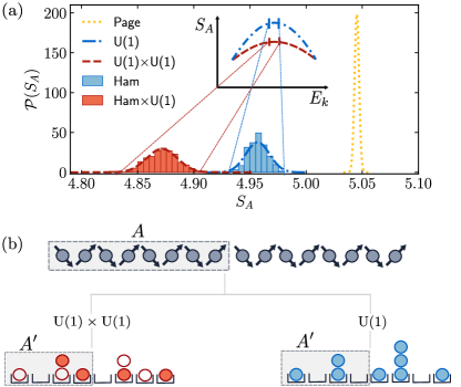
Figure 1: (a) Histograms of half-system entanglement entropy (EE) of mid-spectrum eigenstates for Hamiltonian systems with a scalar U(1) charge (left, red) and for a Hamiltonian system without additional symmetries (right, blue). The lines indicate the EE distribution of pure random states without constraints (dotted), random states with a U(1) constraint (dashed-dotted), and random states with two U(1) constraints (dashed). (b) Schematics showing the coarse-graining procedure used to generate RMT ensembles that capture the entanglement patterns of a spin chain Hamiltonian of spin-$1/2$ qubits, shown for $L=16$. In particular, we consider a chain of $L^{\prime}=L/\lambda$ qudits with local Hilbert space dimension $d^{\prime}=d^{\lambda}$, with $\lambda=2$, and consider random states within a fixed symmetry sector for each U(1) charge. Parameters used in the histograms: $L=16$, $J=1$, $\Delta=J/2$, $J_{2}=0.6$, $h_{x}=0$ (Ham$\times$U(1)), and $h_{x}=0.75$, $J_{2}=0$ (Ham), see Eqs.(Entanglement patterns of quantum chaotic Hamiltonians with a scalar U(1) charge) and (8).

While RMT captures ‘coarse’ features of quantum states in chaotic regimes, it fails to describe their ‘fine’ features. In particular, eigenstates of physical Hamiltonians encode correlations, whereas RMT ensembles do not. In fact, the correlations encoded in a single eigenstate is sufficient to reconstruct the entire Hamiltonian, so long as the Hamiltonian is local [20, 15]. Many recent works have aimed to capture structure in quantum states that goes beyond RMT. For example, Refs. [21, 22, 23, 24, 25, 26, 27] showed that matrix elements of local operators evaluated in the eigenbasis of the Hamiltonian remain correlated up to a particular energy scale related to the so-called Thouless time [8, 28, 29, 9, 10]. These works clarified that correlations are related to an emergent “light cone” in the growth of out-of-time ordered commutators in spatially local systems [25, 26, 27]. Other works have identified systematic deviations between the EE of mid-spectrum Hamiltonian eigenstates and pure random states [30, 31, 32, 33, 17, 34].

Despite all these works, notions of quantum chaos that systematically incorporate additional structure beyond RMT are lacking. The perspective that we take in this letter is to systematically construct RMT ensembles that capture increasingly finer features of typical quantum states of physical Hamiltonians by imprinting additional structure on quantum states, such as spatial locality and symmetries. An initial step in this direction was done in our recent work [35] where we showed that the EE of mid-spectrum eigenstates of local Hamiltonian systems (in the absence of any additional structure) is not described by plain RMT but, instead, by a constrained RMT ensemble that accounts for a U(1) scalar charge [35]—energy in local systems plays the role of the scalar charge. Similar arguments were put forward by Huang [31, 32] to justify deviations from the maximal EE of eigenstates in local Hamiltonian systems.

More generally, here we demonstrate that we can accurately describe the entanglement patterns of eigenstates of physical systems—including their fluctuations—by appropriately constraining the RMT distribution, focusing on Hamiltonian systems with an additional U(1) scalar charge, see Fig.1. Systems with a U(1) scalar charge arise in models of experimental interest, such as magnetic systems, and systems with particle number conservation, such as interacting Fermi and Bose gases [36, 37]. By systematically constructing RMT ensembles that account for conservation of energy and magnetization (or particle number), we accurately describe the ensemble properties of eigenstates beyond their average behavior, both analytically and numerically. Specifically, using this approach, we describe the entanglement patterns of mid-spectrum eigenstates, including their fluctuations, at all lengthscales (Figs.1 and 2).

Ensembles without any constraints.—We consider ensemble properties of eigenstates and pure random states through the lens of EE,

$$S_{A}=-\text{Tr}[\rho_{A}\log(\rho_{A})],$$ (1)

in the context of spin chains comprised of $L$ qudits with local Hilbert space dimension $d$. In Eq.(1), $\rho_{A}={\rm Tr}_{B}[|\Psi\rangle\langle\Psi|]$ is the reduced density matrix of the state $|\Psi\rangle$ when the system is bipartitioned into two subsystems of length $L_{A}=fL$ and $L_{B}=(1-f)L$, each of which has Hilbert space dimension $d_{A}=d^{L_{A}}$ and $d_{B}=d^{L_{B}}$. An ensemble of quantum states $\{|\Psi\rangle\}$ produces a distribution $\mathcal{P}(S_{A})$ of EE, which we aim to describe at the level of higher moments.

For example, in the absence of any structure, the distribution of EE of pure random states $|\Psi\rangle$ drawn from the full Hilbert space $\in{\cal H}$ depends only on subsystem dimensions through the parameters $(f,L)$. In particular, the average EE, $\mu=\langle S_{A}\rangle$, in the asymptotic limit ($L\gg 1$) is given by

$$\mu(L,f)\approx Lf\log d-\frac{1}{2}\delta_{f,1/2},$$ (2)

which was first conjectured by Page [38] and later proven analytically by others [39, 40, 41]. The first term in the RHS of Eq.(2) is the volume-law term which scales with subsytem size $L_{A}=fL$, whereas the second term gives rise to the ‘half-qubit’ shift correction for half-subsystems. The variance of EE for pure random states, $\sigma^{2}_{P}\approx d^{-L(1+|1-2f|)}$, is exponentially small in subsystem size, implying that the EE is typical and a single pure random state will have the Page entropy.

Ensembles constrained by one scalar charge.—Energy conservation in local Hamiltonian systems adds structure into eigenstates which is not described by plain RMT. Although there are subtle differences between energy conservation and U(1) charge conservation, namely, the energy operator is sum of $k$-local terms (typically, $k=2$ or $3$) with a continuously distributed eigenspectrum, we expect that such microscopic differences are washed away when computing the EE for large enough subsystems ($d_{A}\gg 1$). Such arguments were discussed in more detail in our work [35].

For systems with a local scalar charge and a local Hilbert space dimension of $d=2$, it is convenient to think of $0\leq M\leq L$ as an integer particle number, and each site only able to accommodate a maximum of one particle. The Hilbert space ${\mathcal{H}(M)}$ of states with fixed charge $M$ decomposes as a direct sum of tensor products, ${\cal H}(M)=\bigoplus_{M_{A}}{\cal H}_{A}(M_{A})\otimes{\cal H}_{B}(M-M_{A})$, where $M_{A}$ is within the range ${\rm max}(0,M-L_{B})\leq M_{A}\leq{\rm min}(M,L_{A})$. The Hilbert space dimension of ${\cal H}_{A}(M_{A})$ is $d_{A,M_{A}}=\binom{L_{A}}{M_{A}}$, the Hilbert space dimension of ${\cal H}_{\rm B}(M-M_{A})$ is $d_{B,M-M_{A}}=\binom{L-L_{A}}{M-M_{A}}$, and the total Hilbert space dimension is $\sum_{M_{A}}d_{A,M_{A}}d_{B,M-M_{A}}=d_{M}=\binom{L}{M}$. A random state with fixed total charge $|\Psi_{M}\rangle\in{\cal H}(M)$ can be expressed as a superposition of orthonormal basis states, $|\Psi_{M}\rangle=\sum_{M_{A}}\psi_{\alpha,\beta}^{(M_{A})}|M_{A},\alpha\rangle\otimes|M-M_{A},\beta\rangle$, with $\psi^{(M_{A})}_{\alpha,\beta}$ uncorrelated random numbers up to normalization. The index $\alpha$ ($\beta$) labels the basis states in subsystem $A$ ($B$) with a total charge $M_{A}$ ($M-M_{A}$).

The reduced density matrix of subsystem $A$ is block diagonal, $\rho_{A|M}=\sum_{M_{A}}p_{M_{A}}\rho_{A|M_{A}}$, and the factors $p_{M_{A}}\geq 0$ are the (classical) probability distribution of finding $M_{A}$ particles in $A$. The entanglement entropy can be written as

$$S(\rho_{A|M})=\sum_{M_{A}}p_{M_{A}}S(\rho_{A|M_{A}})-p_{M_{A}}\log p_{M_{A}},$$ (3)

where the second term on the RHS is the Shannon entropy of the number distribution $p_{M_{A}}$, which captures particle number correlations between the two subsystems, and the first term captures quantum correlations between configurations with a fixed particle number.

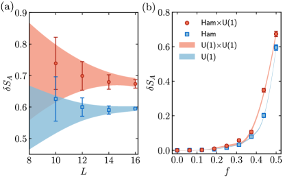
Figure 2: (a) Finite-size scaling of the EE distribution as a function of $L$ for fixed $f=1/2$. The data is shown relative to the maximum entropy, $\delta S_{A}=Lf\log(2)-S_{A}$. The red points indicate the average EE, and the bars indicate the standard deviation of EE. (b) Distribution of EE for mid-spectrum eigenstates as a function of $f$ for fixed $L=16$. The shaded region in panels (a) and (b) are obtained from sampling pure random states with a U(1) constraint (blue) and a U(1)$\times$U(1) constraint (red) in coarse-grained systems of size $L^{\prime}=[4,6,8]$, see Fig.1(b). Parameters used in panels (a) and (b): (red) $J=1$, $\Delta=J/2$, $J_{2}=0.6$, $h_{x}=0$ and (blue) $J_{2}=0$, $h_{x}=0.75$. For small values of $f$, the standard deviation bars are hidden behind the data points.

The first few moments of the EE distribution produced by the ensemble $|\Psi\rangle\in{\cal H}(M)$ was first computed by Bianchi and Dona [41], see details in the Supplement. In particular, the mean entanglement entropy for ‘mid-spectrum’ states (i.e., $M/L=1/2$) in the asymptotic limit is given by

$$\mu_{M}(L,f)=Lf\log(d)+\frac{f+\log(1-f)}{2}-\frac{1}{2}\delta_{f,1/2}.$$ (4)

Interestingly, in addition to the volume-law term and the half-qubit shift, Eq.(4) also exhibits a finite shift in the mean EE entropy relative to the Page result [38]. The variance of EE scales exponentially with system size, $\sigma_{M}\sim\sqrt{L}/d^{L}$, thus a typical pure random state in ${\cal H}(M)$ will have the EE in Eq.(4). We emphasize that the difference between the typical EE of random states in ${\cal H}(M)$ and ${\cal H}$ is significant on the exponentially small scale set by $\sigma_{M}$, see dotted and dashed-dotted lines in Fig.1(a).

We note that if random vectors are real valued (i.e., GOE distributed), which describes states in systems with time-reversal symmetry, the mean EE is not affected at the level of $O(1)$ corrections, but the standard deviation increases by a factor of $\sqrt{2}$ [42, 39]. This is true both for constrained and unconstrained ensembles (see Supplement).

Ensembles constrained by two commuting scalar charges.—We now consider quantum state ensembles constrained by an additional U(1) charge, which is more descriptive of typical quantum states in systems that conserve energy and magnetization. Unlike the U(1) case, there is a technical difficulty in constructing random state ensembles that have two scalar constraints if the local Hilbert space dimension is $d=2$: the symmetry operators for both charges cannot be simultaneously expressed as a sum of single site terms, thus defining a suitable basis to describe the states is challenging. To address this, we use a ‘coarse-graining’ picture in which we increase the local Hilbert space dimension as $d\rightarrow d^{\lambda}$, and decrease the system size as $L\rightarrow L/\lambda$, while keeping the total Hilbert space dimension constant. By ‘enlarging’ the local Hilbert space dimension, we can express the symmetry operators for both U(1) charges in terms of local operators only. Similarly to the energy-conserving-only case, we argue that the entanglement patterns computed for large enough subsystems are insensitive to the coarse-graining procedure—and, in fact, we find that the entanglement patterns are also insensitive when the subsystem is not so large.

For systems constrained by two scalar U(1) charges and a local Hilbert space dimension of $d=2$, we use $\lambda=2$ and define the random states ensemble, $|\Psi_{M,N}\rangle=\sum_{M_{A},N_{A}}\psi_{\alpha,\beta}^{(M_{A},N_{A})}|M_{A},N_{A};\alpha\rangle\otimes\\ |M-M_{A},N-N_{A};\beta\rangle$, with local Hilbert space dimension $d^{\prime}=4$. The numbers $N$ and $M$ represent the quantum numbers of each scalar charge, and each site can accommodate one particle of each flavor, see Fig.1(b). The index $\alpha$ ($\beta$) labels basis states with $M_{A}$ and $N_{A}$ ($M-M_{A}$ and $N-N_{A}$) particles in $A$ ($B$). In this case, the EE of $\rho_{A}$ can be expressed as

$$S(\rho_{A|M,N})=\sum_{M_{A},N_{A}}p_{M_{A},N_{A}}S(\rho_{A|M_{A},N_{A}})$$ (5)

$$-p_{M_{A},N_{A}}\log p_{M_{A},N_{A}},$$

where each term has the same physical meaning as those in Eq.(3). When states are drawn randomly from ${\cal H}(M,N)$, the resulting distribution is computed along the same lines as in the U(1) case, and the details are discussed in the Supplement. We find that the mean EE for mid-spectrum states ($M/L=1/2$ and $N/L=1/2$) in the asymptotic limit is given by,

$$\mu_{M,N}(L,f)=Lf\log(d)+f+\log(1-f)-\frac{1}{2}\delta_{f,1/2}.$$ (6)

In particular, the mean EE is shifted twice the value found in Eq.(4) relative to the Page mean. Note that the mean EE does not change if we rescale $L\rightarrow L/\lambda$ and $d\rightarrow d^{\lambda}$, so long as $f$ remains constant. The variance of EE is exponentially small in systems size, $\sigma_{M,N}\sim L/d^{L}$ (see Supplement). We note that the ratio $\sigma_{M,N}/\sigma_{M}\sim L^{1/4}$; this leads to $\sigma_{M,N}$ being twice as large than $\sigma_{M}$ when $L=16$, as shown in Fig.1(a). Having described the three reference RMT ensembles, we now compare these with ensembles of eigenstates of Hamiltonian systems with and without U(1) symmetry.

Model Hamiltonian.—We consider the spin-1/2 Hamiltonian:

$$H=\sum_{\ell}J\left(X_{\ell}X_{\ell+1}+Y_{\ell}Y_{\ell+1}\right) +\Delta Z_{\ell}Z_{\ell+1}$$

$$+J_{2}Z_{\ell}Z_{\ell+1}Z_{\ell+2},$$ (7)

where $(X_{\ell},Y_{\ell},Z_{\ell})$ are the Pauli matrices. The Hamiltonian (Entanglement patterns of quantum chaotic Hamiltonians with a scalar U(1) charge) has two scalar charges, energy and total magnetization $S_{z}=\sum_{\ell}Z_{\ell}$, both of which are commuting, $[H,S_{z}]=0$. The Hamiltonian (Entanglement patterns of quantum chaotic Hamiltonians with a scalar U(1) charge) also has multiple point symmetries, which we explicitly break. In particular, we use open boundary conditions to break translation symmetry, and we include boundary fields $h_{1}=Z_{1}/4$ and $h_{L}=-Z_{L}/4$ to break inversion symmetry. When $J_{2}=0$, the Hamiltonian (Entanglement patterns of quantum chaotic Hamiltonians with a scalar U(1) charge) becomes the integrable XXZ chain. A finite value of $J_{2}$, instead, breaks integrability. We first consider the parameters $J=1$, $\Delta=J/2$, and $J_{2}=0.6$, which we find to be the values in which eigenstates are most random.

For comparison, we also consider the Hamiltonian

$$H^{\prime}=H+\sum_{\ell}h_{x}X_{\ell},$$ (8)

with an additional transverse field which breaks both U(1) symmetry and integrability. When breaking U(1) symmetry, we use the parameters $h_{x}=0.75$ and $J_{2}=0$.

We now analyze the EE distribution of mid-spectrum eigenstates at half-filling as a function of $L$ and $f$. In Fig. 2(a), we show the EE distribution of mid-spectrum eigenstates as a function of $L$ for fixed $f=1/2$, both for the Hamiltonian (Entanglement patterns of quantum chaotic Hamiltonians with a scalar U(1) charge) with U(1) symmetry (circles) and for the Hamiltonian (8) without U(1) symmetry (squares). Each data point represents the average EE of eigenstates relative to the maximum entanglement entropy $L_{A}\log(2)$, and the bars indicate their standard deviation. The shaded blue area indicates the regions limited by $\mu_{M}\pm\sigma_{M}$ for the RMT ensemble $|\Psi\rangle\in{\cal H}(M)$ using real-valued vectors, and the shaded red area indicates the region limited by $\mu_{M,N}\pm\sigma_{M,N}$ for the ensemble $|\Psi\rangle\in{\cal H}(M,N)$ also using real-valued vectors (the boundaries are interpolated smoothly between the accessible $L$ values). We obtain the eigenstate distributions by choosing an energy window, $W=20,50,100,600$ of eigenstates for $L=10,12,14,16$ around the peak density-of-states. The entanglement bipartition is placed in the center of the chain to prevent edge effects from the open boundary conditions. For the first and second moments of the EE distribution, we find excellent quantitative agreement between the eigenstate distribution and the corresponding constrained RMT ensemble. This applies both for the Hamiltonian with a U(1) scalar charge and the Hamiltonian without additional structure.

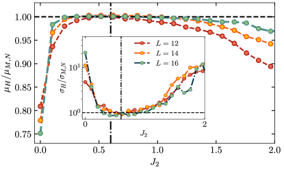
Figure 3: Finite-size scaling of the average EE of mid-spectrum eigenstates relative to the RMT prediction $\mu_{M,N}$ plotted as a function of the integrability breaking parameter $J_{2}$. The inset shows the standard deviation of EE of mid-spectrum eigenstates relative to the RMT prediction $\sigma_{M,N}$. Excellent agreement with the constrained RMT ensemble (at the level of the first two moments) is found only in a small pocket of model parameters centered around $J_{2}\approx 0.6$. Parameters used: $J=1$, $\Delta=J/2$, $h_{x}=0$, $f=1/2$.

For subsystems with $f<1/2$, we also find that the entanglement patterns of mid-spectrum eigenstates are described remarkably well by the constrained RMT ensembles. This is shown in Fig. 2(b) for fixed $L=16$, using the same number of eigenstates as in panel(a).

Whereas previous works have made important steps in highlighting deviations from maximal entropy of eigenstates in Hamiltonian systems with a U(1) charge[19, 43], with deviations qualitatively captured by the ensemble $|\Psi\rangle\in{\cal H}(M)$, clear differences between the eigenstate and the U(1)-constrained RMT ensembles are visible when both ensembles are compared on the microscopic scale given by the entropy fluctuations $\sigma_{M}$. In particular, we find that the typical EE of eigenstates in Hamiltonian systems with a U(1) charge is several standard deviations away from the U(1)-constrained RMT ensemble, as shown in Figs.1 and 2. Overall, the presence of two local charges—energy and magnetization—effectively constrains the available phase space, leading to quantitatively distinct patterns of entanglement at the level of first and second moments.

Maximally chaotic systems.—In Figs. 1 and 2, we set the next nearest-neighbor term $J_{2}=0.6$, which we found to be the value where eigenstates are most random. In Ref. [35], we conjectured the existence of ‘maximally chaotic’ Hamiltonians at fined tuned regions of parameter space where the distance to the appropriately constrained RMT ensembles is minimal. The model used in Ref. [35] was the Mixed Field Ising Model, with the higher moments of the EE minimizing and agreeing with RMT ensembles in small pockets of parameter space. We reach the same conclusion in a completely different model, as shown in Fig. 3. For instance, by tuning $J_{2}$ away from $J_{2}=0.6$ [vertical dashed line], we find systematic deviations from the constrained RMT ensembles that persist in the thermodynamic limit. In particular, eigenstates and constrained RMT states exhibit the same patterns of entanglement at the level of first and second moments when $J_{2}\approx 0.6$. As we depart from $J_{2}\approx 0.6$, there is a decrease in the average entanglement and an increase in their fluctuations that persist in the thermodynamic limit.

Discussion.—Our work shows that constrained RMT ensembles can describe increasingly finer features of eigenstates in physical systems, with key system properties captured by appropriate constraints. This sharpens our understanding of quantum chaos and its connection with RMT. This also shows the need to characterize new classes of constrained RMT ensembles to understand the universal properties of eigenstates in physical systems with additional symmetries. An interesting direction for future research is describing the fine features of EE in the presence of non-abelian symmetries [44, 45]. On a different front, our work strengthens our claim in Ref. [35], suggesting a notion of ‘maximal chaos’ in local physical systems in fined-tuned pockets of parameter space. In particular, ensembles of eigenstates are indistinguishable from appropriately-constrained RMT ensembles at the level of subsystem entropies only in small pockets of parameter space. An interesting question is, what conditions are required to maximize chaos in local systems, and what are the dynamical signatures of these ‘maximally chaotic’ Hamiltonians?

Acknowledgements.—We thank Vedika Khemani and Cheryne Jonay for previous collaborations and feedback on the present work, as well as Nick Hunter-Jones and Sam Garratt for helpful discussions. JFRN acknowledges the hospitality of the Aspen Center for Physics, which is supported by National Science Foundation grant PHY-2210452, and where this work was initiated. The numerical simulations in this work were conducted with the advanced computing resources provided by Texas A&M High Performance Research Computing.

This Supplementary Material discusses the analytical and numerical details of the results presented in the main text. Section S1 discusses the entanglement entropy (EE) distributions generated by constrained and unconstrained random matrix theory (RMT) ensembles. Section II focuses on the statistical analysis of the numerical data.

S1 Entanglement entropy distribution for ensembles of pure random states

In this section, we consider the statistical properties of the EE for various RMT ensembles, both constrained and unconstrained. We start by discussing the case of pure random states without constraints, and then discuss the cases with U(1) and U(1)$\times$U(1) constraints. In all cases, we discuss the exact analytical results as well as the asymptotic behavior, which were discussed in the main text. We finally discuss differences between ensembles drawn from complex valued distributions (GUE) and real valued distributions (GOE).

S1.1 Pure random states without constraints

The first few moments of the EE distribution was first computed analytically in Refs. [39, 40]. In the following, we summarize the key results. Suppose that a system of size $L$ is partitioned into regions $A$ and $B$ of size $L_{A}$ and $L_{B}=L-L_{A}$, with Hilbert space dimensions $d_{A}=d^{L_{A}}$ and $d_{B}=d^{L_{B}}$, respectively. We assume without loss of generality that $L_{A}\leq L_{B}$. A pure state $\ket{\psi}$ on the full Hilbert space $\mathcal{H}=\mathcal{H}_{A}\otimes\mathcal{H}_{B}$ can be expressed as

$$\ket{\psi}=\sum_{\alpha=1}^{d_{A}}\sum_{\beta=1}^{d_{B}}\psi_{\alpha,\beta}\ket{\alpha}\otimes\ket{\beta},$$ (S1)

where $|\alpha\rangle$ ($|\beta\rangle$) are basis states of subsystem $A$ ($B$), and the coefficients $\psi_{\alpha,\beta}$ represent entries of a rectangular matrix of dimension $d_{A}\times d_{B}$. Tracing out the degrees of freedom of subsystem $B$, the reduced density matrix can be written as

$$\rho_{A} =\sum_{\alpha,\alpha^{\prime}=1}^{d_{A}}\left[\sum_{\beta=1}^{d_{B}}\psi_{\alpha,\beta}\psi^{*}_{\alpha^{\prime},\beta}\right]\ket{\alpha}\bra{\alpha^{\prime}}.$$ (S2)

The EE of $\rho_{A}$, $S(\rho_{A})=-{\rm Tr}[\rho_{A}\log\rho_{A}]$ is obtained from the eigenspectrum $\{\lambda_{\alpha}\}$ of $\rho_{A}$, specifically, $S_{A}=-\sum_{\alpha}\lambda_{\alpha}\log(\lambda_{\alpha})$.

Let us now consider coefficients $\psi_{\alpha,\beta}$ which are independently and identically distributed complex (GUE) Gaussian variables drawn from the distribution $\mathcal{P}(\psi)=\exp\{-\text{Tr}[\psi^{{\dagger}}\psi]\}$. This generates a distribution of EE ${\cal P}(S_{A})$ with average $\mu=\langle S_{A}\rangle$ given by[39, 40]

$$\mu=\Psi(d_{A}d_{B}+1)-\Psi(d_{B}+1)-\frac{d_{A}-1}{2d_{B}},$$ (S3)

where $\Psi(x)=\Gamma(x)^{\prime}/\Gamma(x)$ is the digamma function, defined as the logarithmic derivative of the Gamma function. When $L_{A}>L_{B}$, one needs to swap $d_{A}\leftrightarrow d_{B}$. The second moment of the EE distribution, $\sigma=\langle S_{A}^{2}\rangle-\langle S_{A}\rangle^{2}$, is given by:

$$\sigma^{2} =\frac{d_{A}+d_{B}}{d_{A}d_{B}+1}\Psi^{\prime}(d_{B}+1)-\Psi^{\prime}(d_{A}d_{B}+1)$$

$$-\frac{(d_{A}-1)(d_{A}+2d_{B}-1)}{4d_{B}^{2}(d_{A}d_{B}+1)},$$ (S4)

where $\Psi^{\prime}(x)=d\Psi(x)/dx=d^{2}[\log(\Gamma(x))]/dx^{2}$ is the first derivative of the digamma function (i.e., the first polygamma function).

S1.1.1 Asymptotic limit: unconstrained states

We now consider $\mu$ and $\sigma$ in the thermodynamic limit $L\gg 1$. Assuming $f=L_{A}/L$ to be a finite fraction of the system, and $d_{A},d_{B}\gg 1$, we can approximate $\Gamma(x\gg 1)\approx\log x$ and $\Gamma^{\prime}(x)\approx 1/x$. In addition, the second term in Eq.(S3), $(d_{A}-1)/2d_{B}$ is finite only if $L_{A}=L_{B}$. In this case, the first moment (S3) takes the form,

$$\mu\approx Lf\log d-\frac{1}{2}\delta_{f,1/2}.$$ (S5)

The first term in Eq.(S5) is the volume law term proportional to $L_{A}$, and the second term is the so-called Page correction, which is exponentially small for $f<1/2$. The variance of the distribution ${\cal P}(S_{A})$ scales as

$$\sigma^{2}\approx\frac{1}{d_{B}^{2}}=d^{-L(1+|1-2f|)},$$ (S6)

which is exponentially small in subsystem size. This implies that the EE is typical and a single pure random state will have the Page entropy.

S1.2 Pure random states with a scalar U(1) constraint

The statistical properties of EE for pure random states constrained to a U(1) symmetry sector was first derived by Bianchi and Dona [41]. An excellent review is presented in Ref. [19]. Here we quote the main results which are relevant to our work.

Let us consider a chain of $L$ sites and a total number of $M$ particles, with $0\leq M\leq L$, and each site able to accommodate a maximum of one particle. When the system is partitioned into two subsystems of sizes $L_{A}$ and $L_{B}$, the Hilbert space factors out as

$$\mathcal{H}(M)=\bigoplus_{M_{A}={\rm max}(0,M-L_{B})}^{{\rm min}(M,L_{A})}\mathcal{H}_{A}(M_{A})\otimes\mathcal{H}_{B}(M-M_{A}).$$ (S7)

The total Hilbert space dimension of each $M$ particle sector is $d_{M}=\binom{L}{M}$, and the Hilbert space dimensions of each subsystem are $d_{M_{A}}=\binom{L_{A}}{M_{A}}$ and $d_{M_{B}}=\binom{L-L_{A}}{M-M_{A}}$.

We now consider random states $|\Psi_{M}\rangle\in{\cal H}(M)$,

$$|\Psi_{M}\rangle=\sum_{M_{A}}\sum_{\alpha,\beta}\psi_{\alpha,\beta}^{(M_{A})}|M_{A},\alpha\rangle\otimes|M-M_{A},\beta\rangle,$$ (S8)

with coefficients $\psi_{\alpha,\beta}^{(M_{A})}$ which are independently and identically distributed complex (GUE) Gaussian variables. The reduced density matrix of subsystem $A$ is block diagonal, $\rho_{A|M}=\sum_{M_{A}}p_{M_{A}}\rho_{A|M_{A}}$, and the factors $p_{M_{A}}\geq 0$ are the (classical) probabilities of finding $M_{A}$ particles in $A$, $p_{M_{A}}=\frac{d_{M_{A}}d_{M_{B}}}{d_{M}}$.

The EE can be written as

$$S(\rho_{A|M})=\sum_{M_{A}}p_{M_{A}}S(\rho_{A|M_{A}})-p_{M_{A}}\log p_{M_{A}},$$ (S9)

where the second term on the RHS is the Shannon entropy of the number distribution $p_{M_{A}}$, which captures particle number correlations between the two halves, while the first term is the Page entropy for the block with $M_{A}$ particles in subsystem $A$.

The first moment of EE, $\mu_{M}=\langle S_{A}\rangle_{M}$, is given by[41]

$$\mu_{M}= \sum_{M_{A}}p_{M_{A}}\phi_{M_{A}},$$ (S10)

$$\phi_{M_{A}}= \Psi(d_{M}+1)-\Psi(\max(d_{M_{A}},d_{M_{B}})+1)$$

$$-\min\left(\frac{d_{M_{A}}-1}{2d_{M_{B}}},\frac{d_{M_{B}}-1}{2d_{M_{A}}}\right).$$ (S11)

In other words, the mean EE of states in a given U(1) symmetry sector is the Page entropy for all random blocks $\rho_{A|M_{A}}$ averaged with $p_{M_{A}}$.

The variance of the entanglement distribution for complex random states restricted to a symmetry sector $M$ is given by:

$$\sigma_{M}^{2}=\frac{1}{d_{M}+1}\bigg{[}\sum_{M_{A}}p_{M_{A}}\left(\phi_{M_{A}}^{2}+\chi_{M_{A}}\right)-\langle S_{A}\rangle_{M}^{2}\bigg{]},$$ (S12)

where $p_{M_{A}}$, and $\phi_{M}$ are defined in the previous equations, and $\chi_{M}$ for $d_{A}\leq d_{B}$ takes the form,

$$\chi_{M_{A}}=\begin{cases}(d_{M_{A}}+d_{M_{B}})\Psi^{\prime}(d_{M_{B}}+1)-(d_{M}+1)\Psi^{\prime}(d_{M}+1)-\frac{(d_{M_{A}}-1)(d_{M_{A}}+2d_{M_{B}}-1)}{4d^{2}_{M_{B}}},\quad\text{if $d_{M_{A}}\leq d_{M_{B}}$}\\ (d_{M_{A}}+d_{M_{B}})\Psi^{\prime}(d_{M_{A}}+1)-(d_{M}+1)\Psi^{\prime}(d_{M}+1)-\frac{(d_{M_{B}}-1)(d_{M_{B}}+2d_{M_{A}}-1)}{4d^{2}_{M_{A}}},\quad\text{if $d_{M_{A}}>d_{M_{B}}$}.\end{cases}$$ (S13)

S1.2.1 Asymptotic limit: U(1) constraint

We now consider the thermodynamic limit $L\gg 1$, and define the particle density $m=M/L$, the subsystem density $m_{A}=M_{A}/L$, and the subsystem fraction $f=L_{A}/L$. In this case, the average value of $m_{A}$ is $\bar{m}_{A}=fm$. Assuming $d_{A},d_{B}\gg 1$, we can replace the Gamma functions by $\Gamma(x\gg 1)\approx\log x$, and use the Stirling’s approximation to approximate the binomial coefficients,

$$\log\binom{L}{M} \approx-L[m\log(m)+(1-m)\log(1-m)]$$

$$+\frac{1}{2}\log\left[\frac{L}{M(L-M)}\right]+\frac{1}{2}\log(2\pi).$$ (S14)

Using these approximations, the terms $p_{M_{A}}$ and $\phi_{M_{A}}$ in Eq.(S10) can be expressed in powers of $(m_{A}-\bar{m}_{A})$ around $\bar{m}_{A}$ in order to compute $\mu_{M}$ up to O(1) terms. The probability distribution of $m_{A}$ is Gaussian-distributed,

$$p_{m_{A}}=$$

$$\sqrt{\frac{2\pi L}{m(1-m)f(1-f)}}\exp\bigg{[}-\frac{L}{2}\frac{(m_{A}-fm)^{2}}{m(1-m)f(1-f)}\bigg{]},$$ (S15)

peaked at $\bar{m}_{A}=f{m}$, and has a standard deviation given by $\sigma_{m_{A}}=\sqrt{m(1-m)f(1-f)/L}$.

Using $\Gamma(x\gg 1)\approx\log x$, the term $\phi_{M_{A}}$ in Eq.(S11) can first be approximated as

$$\phi_{M_{A}}=\log\left(\frac{d_{M}}{d_{M_{B}}}\right)-\frac{1}{2}\delta_{f,1/2}\delta_{m,1/2}.$$ (S16)

Using Stirling’s approximation, $\phi_{M_{A}}$ is found to be

$$\phi_{M_{A}}\approx-L[m\log(m)+(1-m)\log(1-m)] +L[m_{B}\log(m_{B})+(1-f-m_{B})\log(1-f-m_{B})-(1-f)\log(1-f)]$$

$$+\frac{1}{2}\log\bigg{[}\frac{m_{B}(1-f-m_{B})}{m(1-m)(1-f)}\bigg{]}-\frac{1}{2}\delta_{f,1/2}\delta_{m,1/2}.$$ (S17)

The last step is integrating $\phi_{m_{A}}$ using the Gaussian distribution $p_{m_{A}}$. In this work, we primarily focus on mid-spectrum states, thus, we set $m=1/2$. In this case, the mean EE up to O(1) terms is given by

$$\mu_{M}(L,f)=Lf\log(d)+\frac{f+\log(1-f)}{2}-\frac{1}{2}\delta_{f,1/2}.$$ (S18)

The same procedure can be applied to the standard deviation $\sigma_{M}$ in Eq.(S12). We note that the term in brackets in Eq.(S12) is O(1), thus the system size dependence of $\sigma_{M}^{2}$ is dominated by the term $d_{M}$ in the denominator. The value of $\sigma_{M}^{2}$ can then be approximated as

$$\sigma_{M}^{2}\approx\frac{1}{d_{M}}\sim\frac{\sqrt{L}}{2^{L}},$$ (S19)

where the numerical prefactor of $\sigma_{M}^{2}$ depends on $f$. Unlike that Page variance $\sigma^{2}$ in Eq.(S6), however, here we note that $\sigma_{M}^{2}$ is a factor $\sqrt{L}$ larger than $\sigma^{2}$. This is because $d_{M}={L\choose M}$ is a factor $\sqrt{L}$ smaller than $d^{L}$ in the asymptotic limit.

S1.3 Pure random states with two scalar U(1)$\times$U(1) constraints.

We now discuss the distribution of EE of pure random states with a U(1)$\times$ U(1) constraint, defined by a Hilbert space, $\mathcal{H}(M,N)$ with a fixed number of particles $M$ and $N$. Let us consider a system of $L$ sites with a local Hilbert space dimension $d=4$, with the local basis states spanned by either an empty site, a site occupied by particle-$1(2)$ or occupied by both particles [see Fig. (1)(b) in the main text]. The Hilbert space dimension of a symmetry sector with $(M,N)$ particles is

$$d_{M,N}=\binom{L}{M}\binom{L}{N},$$ (S20)

with $\sum_{M,N=0}^{L}\binom{L}{M}\binom{L}{N}=4^{L}$ by Vandermonde’s identity. We next bipartition the system into $A$ and $B$ subregions of size $L_{A}$ and $L_{B}=L-L_{A}$. In this case, the Hilbert space of the $(M,N)$ symmetry sector decomposed as

$$\mathcal{H}(M,N)=$$

$$\bigoplus_{M_{A},N_{A}} \mathcal{H}_{A}(M_{A},N_{A})\otimes\mathcal{H}_{B}(M-M_{A},N-N_{A}),$$ (S21)

where the Hilbert space dimension of subsystem $A$ with $(M_{A},N_{A})$ particles is given by $d_{M_{A},N_{A}}=\binom{L_{A}}{M_{A}}\binom{L_{A}}{N_{A}}$, and the Hilbert space dimension of subsystem $B$ with $(M_{B},N_{B})$ particles is given by $d_{M_{B},N_{B}}=\binom{L-L_{A}}{M-M_{A}}\binom{L-L_{A}}{N-N_{A}}$.

Let us consider a state $\ket{\Psi}\in\mathcal{H}(M,N)$

$$\ket{\psi}=\sum_{M_{A},N_{A}}\sum_{\alpha,\beta}\psi^{(M_{A},N_{A})}_{\alpha,\beta} \ket{M_{A},N_{A},\alpha}$$

$$\otimes\ket{M-M_{A},N-N_{A},\beta},$$ (S22)

with the coefficients $\psi_{\alpha,\beta}^{(M_{A},N_{A})}$ independently and identically distributed complex (GUE) Gaussian variables. Here $|M_{A},N_{A},\alpha\rangle$ ($|M_{B},N_{B},\beta\rangle$) are basis states of subsystem $A$ ($B$) with $(M_{A},N_{A})$ [($M_{B},N_{B}$)] particles. The reduced density matrix of the above state over subsystem $A$ is of block diagonal form, namely,

$$\rho_{A}=\sum_{M_{A},N_{A}}p_{M_{A},N_{A}}\rho_{A|M_{A},N_{A}}.$$ (S23)

The values $p_{M_{A},N_{A}}$ come from normalizing the reduced density matrix within in each $(M_{A},N_{A})$ sector and satisfy $\sum_{M_{A},N_{A}}p_{M_{A},N_{A}}=1$. The factors $p_{M_{A},N_{A}}$ are interpreted as the classical probability of finding $M_{A}$ and $N_{A}$ particles over the subregion $A$. Moreover, the entanglement entropy becomes

$$S(\rho_{A})=\sum_{M_{A},N_{A}}p_{M_{A},N_{A}} S(\rho_{A|M_{A},N_{A}})$$

$$-p_{M_{A},N_{A}}\log(p_{M_{A},N_{A}}),$$ (S24)

where the second term is the Shannon entropy which captures classical correlations between particles of the subsystems, while the first term captures quantum correlations. Importantly, since the two $U(1)$ charges commute, we assume that $p_{M_{A},N_{A}}=p_{M_{A}}p_{N_{A}}$ are independent probabilities for each flavor. In addition, each block $\rho_{A|M_{A},N_{A}}$ with $(M_{A},N_{A})$ particles is assumed to be a random matrix. In this case, $S(\rho_{A|M_{A},N_{A}})$ is the Page entropy (S3) for pure random strained constrained to $(M_{A},N_{A})$ particles in subsystem $A$. Thus, the average EE $\mu_{M,N}=\langle S_{A}\rangle_{M,N}$ for pure random states in the $(M,N)$ symmetry sector is the Page entropy for each block $\rho_{A|M_{A},N_{A}}$ averaged with the distribution $p_{M_{A},N_{A}}$,

$$\mu_{M,N} =\sum_{M_{A},N_{A}}\frac{d_{M_{A},N_{A}}d_{M_{B},N_{B}}}{d_{M,N}}\phi_{M_{A},N_{A}}$$ (S25)

$$\phi_{M_{A},N_{A}} =\Psi(d_{M,N}+1)-\Psi(\max(d_{M_{A},N_{A}},d_{M_{B},N_{B}})+1)$$

$$-\min\bigg{[}\frac{d_{M_{A},N_{A}}-1}{2d_{M_{B},N_{B}}},\frac{d_{M_{B},N_{B}}-1}{2d_{M_{A},N_{A}}}\bigg{]},$$

with $\Psi(z)=\Gamma^{\prime}(z)/\Gamma(z)$ the Digamma function, and $d_{A(B)}$ defined above. The variance of the entanglement distribution for complex random states restricted to a symmetry sector $(M,N)$ is given by:

$$\sigma_{M,N}^{2} =\frac{1}{d_{M,N}+1}\bigg{[}\sum_{M_{A},N_{A}}p_{M_{A},N_{A}}\left(\phi_{M_{A},N_{A}}^{2}+\chi_{M_{A},N_{A}}\right)$$

$$-\langle S_{A}\rangle_{M,N}^{2}\bigg{]},$$ (S26)

where $p_{M_{A},N_{A}}=\frac{d_{M_{A},N_{A}}d_{M_{B},N_{B}}}{d_{M,N}}$, and $\phi_{M_{A},N_{A}}$ are defined in the previous equations, and $\chi_{M_{A},N_{A}}$ takes the form,

$$\chi_{M_{A},N_{A}}=\begin{cases}(d_{M_{A},N_{A}}+d_{M_{B},N_{B}})\Psi^{\prime}(d_{M_{B},N_{B}}+1)-(d_{M,N}+1)\Psi^{\prime}(d_{M,N}+1)-\frac{(d_{M_{A},N_{A}}-1)(d_{M_{A},N_{A}}+2d_{M_{B},N_{B}}-1)}{4d^{2}_{M_{B},N_{B}}},\\ \\ (d_{M_{A},N_{A}}+d_{M_{B},N_{B}})\Psi^{\prime}(d_{M_{A},N_{A}}+1)-(d_{M,N}+1)\Psi^{\prime}(d_{M,N}+1)-\frac{(d_{M_{B},N_{B}}-1)(d_{M_{B},N_{B}}+2d_{M_{A},N_{A}}-1)}{4d^{2}_{M_{A},N_{A}}}.\end{cases}$$ (S27)

Where case 1: $d_{M_{A},N_{A}}\leq d_{M_{B},N_{B}}$, and case 2: $d_{M_{A},N_{A}}>d_{M_{B},N_{B}}$.

S1.3.1 Asymptotic limit: U(1)$\times$U(1) constraint

We now consider the asymptotic limit $L\gg 1$, and define the particle densities $m=M/L$, $n=N/L$, $m_{A}=M_{A}/L$, $n_{A}=N_{A}/L$, and the subsystem fraction as $f=L_{A}/L$. In this case, the average value of $m_{A}$ and $n_{A}$ is $\bar{m}_{A}=fm$ and $\bar{n}_{A}=fn$. Because $d_{A},d_{B}\gg 1$, we can also replace the Gamma functions by $\Gamma(x\gg 1)\approx\log x$, and use the Stirling’s approximation in Eq.(S14) to approximate the binomial coefficients. For each symmetry sector, the probability distributions acquire a Gaussian form like in Eq.(S1.2.1). In addition, the asymptotic form of the term $\phi_{M_{A},N_{A}}$ is

$$\phi_{M_{A},N_{A}}=\log\left(\frac{d_{M}}{d_{M_{B}}}\frac{d_{N}}{d_{N_{B}}}\right)-\frac{d_{M_{A}}d_{N_{A}}-1}{2d_{M}d_{N}}.$$ (S28)

Putting everything together into the expression for $\mu_{M,N}$, we obtain

$$\mu_{M,N}=\sum_{M_{A},N_{A}}p_{M_{A}}p_{N_{A}}\left[\log\left(\frac{d_{M}}{d_{M_{B}}}\frac{d_{N}}{d_{N_{B}}}\right)-\right.$$ (S29)

$$\left.\frac{d_{M_{A}}d_{N_{A}}-1}{2d_{M}d_{N}}\right]$$

Because we assume the distributions $p_{M_{A}}$ and $p_{N_{A}}$ to be independent, the average entanglement entropy separates into two equivalent expressions

$$\langle S_{A}\rangle_{M,N}=\sum_{M_{A}}p_{M_{A}}\log\left(\frac{d_{M}}{d_{M_{B}}}\right)+\sum_{N_{A}}p_{N_{A}}\log\left(\frac{d_{N}}{d_{N_{B}}}\right)$$ (S30)

$$-\frac{1}{2}\delta_{f,1/2}\delta_{m,1/2}\delta_{n,1/2},$$

after using $\sum_{M_{A}}p_{M_{A}}=1$, and $\sum_{M_{B}}p_{M_{B}}=1$. Each of the sums can be solved in exactly the same way as described in the previous section.

When evaluating for pure random states with $m=n=1/2$, the average EE in the asymptotic limit is

$$\mu_{M,N}\approx Lf\log(d)+f+\log(1-f)-\frac{1}{2}\delta_{f,1/2}.$$ (S31)

In this case, we find twice the EE shift (relative to the Page value) compared to that found in Eq.(S18).

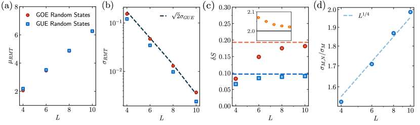
Figure S1: (a) System-size dependence of the average entanglement entropy of pure random states drawn from a GUE (blue) and GOE (red) distribution in the presence of a U(1)$\times$U(1) constraint. In the asymptotic limit, both are converging to the same result. (b) Numerical data for the standard deviations of the entanglement entropy using the same random pure states generated in panel (a). The dotted line shows that the standard deviation of EE of real random states is a factor $\sqrt{2}$ larger than that of complex random states [35]. (c) The deviation from maximal EE, $S_{max}=L\log(2)-0.5$ at $f=1/2$ for both U(1)$\times$U(1) (red) and U(1) (blue) constraints. The U(1)$\times$U(1) case converges to $|f+\log(1-f)|=0.19$, which is two times larger than $|(f+\log(1-f))/2|=0.096$ for the U(1) constraint. Inset: The ratio of the red and blue points showing convergence to the value 2. (d) Standard deviation of EE for pure random states with a U(1)$\times$U(1) constraint relative to that of pure random states with a U(1) constraint. Parameters used: The number of random states for $L=4,6,8,10$ are $10^{6},10^{6},10^{5},10^{4}$.

In the main text, we argue that, in the case of systems with two local scalar charges and Hilbert space dimension $d=2$, one can ‘coarse-grain’ the system as $L^{\prime}=L/\lambda$ and $d^{\prime}=d^{\lambda}$ and, effectively, one obtains the same entanglement patterns as in the unrescaled system. We note that Eq.(S31) is invariant to rescaling. In particular, the volume law term remains invariant upon rescaling, $(L/\lambda)f\log(d^{\lambda})=Lf\log(d)$, and the same occurs for the O(1) terms so long as the subsystem fraction $f$ remains constant. Finally, we comment on the standard deviation of the EE in a system with a U(1)$\times$U(1) charge in the case of half-filling. Similarly to the U(1) case, the variance scales with the inverse of the Hilbert space size of the symmetry sector $(M,N)$, thus

$$\sigma_{M,N}^{2}\approx\frac{1}{d_{M,N}}\sim\frac{L}{d^{L}},$$ (S32)

Unlike the variance $\sigma_{M}^{2}$ in Eq.(S19), however, here we note that $\sigma_{M,N}^{2}$ is a factor ${L}$ larger than $d^{L}$ due to the midspectrum symmetry sector $d_{M,N}$ being a factor $1/L$ smaller than the dimension of the full Hilbert space. As such, we find that that $\sigma_{M,N}/\sigma_{M}\sim L^{1/4}$, see Fig.S1(d).

S2 Numerical Methods.

This section gives details on the numerical procedures used to analyze the numerical data in the main text. First, we go over constructing random pure states drawn from either a GOE or GUE ensemble and discuss how the second moment changes depending on which random matrix ensemble is used. Second, we discuss how to pick a proper window size of infinite temperature states before finite-temperature state become relevant.

S2.1 Random Pure State Entanglement

In Fig. (S1), we numerically compare the first two moments of the entanglement distribution for different system sizes using the random states in Eq. (S1.3) where the $\psi_{\alpha,\beta}^{(M_{A},N_{A})}$ are drawn either from a GUE or GOE ensemble. While exact expressions for the first moments differ between GUE and GOE, they are asymptotically the same in the thermodynamic limit [39, 46, 42]. Fig. S1(a) confirms that there is little difference between the average entanglement values. Figure S1(b) also shows that the standard deviation of $\sigma_{M,N}$(GUE) is a factor $\sqrt{2}$ larger than $\sigma_{M,N}$(GOE) (shown by the blue dashed line). The additional prefactor is due to averaging over both the real and complex parts of the GUE ensemble.

In Fig. S1 (c) we isolate the $O(1)$ correction to the average EE for both a single and two scalar charges using pure random states. Specifically, we compute EE relative to the Page entanglement entropy, $S_{A}\log(2)-0.5$. We find that, as the system size grows in size, the difference approaches either $|f+\log(1-f)|$ for two scalar charges (red) or $|f+\log(1-f)|/2$ for a single charge (blue). The variance of the EE distribution are exponentially small [see above], but the standard deviation has a polynomial scaling with system size relative to $\sigma$, see Eq.(S1.1), which we illustrate in Fig. S1(d).

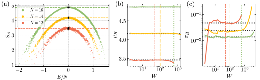
Figure S2: (a) Eigenstate entanglement entropy of the Hamiltonian with two U(1) charges. The black points are the eigenstates used in averaging for that system size. The dashed horizontal lines are the average values from random pure states. (b) Mean and (c) standard deviation of the entanglement distribution as a function of the window size, $W$. Shown with vertical lines is the number $W=50,100,600$ used in averaging in the main-text. Black horizontal lines are the average entanglement from pure random state averages. Parameters in all panels: $J=1$, $\Delta=J/2$, $J_{2}=0.62$, $J_{x}=0$ for $f=1/2$.

S2.2 Window Size Dependence on Distribution Moments

For the Hamiltonian in Eq.(Entanglement patterns of quantum chaotic Hamiltonians with a scalar U(1) charge) of the main text, when computing the first two moments of the EE distribution for mid-spectrum eigenstates, it is necessary to take a finite energy window $\Delta E$ in which to take samples of $S_{A}$, see Fig. S2(a). If the energy window is too small, then a statistically small number of states will be available for sampling, thus leading to large error bars. On the other hand, if the window is too large, then finite-energy eigenstates with low entanglement will skew the distribution and increase its variance, see Figs.S2(c). Because of typicality, we argue only a few eigenstates are necessary to quantify the mean and standard deviation. In Fig. S2 (a) we plot the eigenstate entanglement of the full spectrum for different system sizes, highlighting the set of eigenstates used to construct the microcanonical average [indicated with vertical lines in (b) and (c)].

References

- Deutsch [1991] J. M. Deutsch, Quantum statistical mechanics in a closed system, Physical Review A 43, 2046 (1991).
- Srednicki [1994] M. Srednicki, Chaos and quantum thermalization, Physical Review E 50, 888 (1994).
- Rigol et al. [2008] M. Rigol, V. Dunjko, and M. Olshanii, Thermalization and its mechanism for generic isolated quantum systems, Nature 452, 854 (2008).
- Nandkishore and Huse [2015] R. Nandkishore and D. A. Huse, Many-body localization and thermalization in quantum statistical mechanics, Annu. Rev. Condens. Matter Phys. 6, 15 (2015).
- Atas et al. [2013a] Y. Y. Atas, E. Bogomolny, O. Giraud, and G. Roux, Distribution of the ratio of consecutive level spacings in random matrix ensembles, Phys. Rev. Lett. 110, 084101 (2013a).
- Atas et al. [2013b] Y. Atas, E. Bogomolny, O. Giraud, P. Vivo, and E. Vivo, Joint probability densities of level spacing ratios in random matrices, Journal of Physics A: Mathematical and Theoretical 46, 355204 (2013b).
- Oganesyan and Huse [2007] V. Oganesyan and D. A. Huse, Localization of interacting fermions at high temperature, Physical Review B 75, 155111 (2007).
- Bertini et al. [2018] B. Bertini, P. Kos, and T. Prosen, Exact spectral form factor in a minimal model of many-body quantum chaos, Phys. Rev. Lett. 121, 264101 (2018).
- Chan et al. [2018a] A. Chan, A. De Luca, and J. Chalker, Spectral statistics in spatially extended chaotic quantum many-body systems, Physical Review Letters 121, 060601 (2018a).
- Friedman et al. [2019] A. J. Friedman, A. Chan, A. De Luca, and J. T. Chalker, Spectral statistics and many-body quantum chaos with conserved charge, Phys. Rev. Lett. 123, 210603 (2019).
- Srednicki [1999] M. Srednicki, The approach to thermal equilibrium in quantized chaotic systems, Journal of Physics A: Mathematical and General 32, 1163 (1999).
- D’Alessio et al. [2016] L. D’Alessio, Y. Kafri, A. Polkovnikov, and M. Rigol, From quantum chaos and eigenstate thermalization to statistical mechanics and thermodynamics, Advances in Physics 65, 239 (2016).
- Deutsch [2018] J. M. Deutsch, Eigenstate thermalization hypothesis, Reports on Progress in Physics 81, 082001 (2018).
- Dymarsky et al. [2018] A. Dymarsky, N. Lashkari, and H. Liu, Subsystem ETH, Physical Review E 97, 012140 (2018).
- Garrison and Grover [2018] J. R. Garrison and T. Grover, Does a single eigenstate encode the full hamiltonian?, Phys. Rev. X 8, 021026 (2018).
- Lu and Grover [2019] T.-C. Lu and T. Grover, Renyi entropy of chaotic eigenstates, Phys. Rev. E 99, 032111 (2019).
- Vidmar and Rigol [2017] L. Vidmar and M. Rigol, Entanglement entropy of eigenstates of quantum chaotic hamiltonians, Phys. Rev. Lett. 119, 220603 (2017).
- Murthy and Srednicki [2019] C. Murthy and M. Srednicki, Structure of chaotic eigenstates and their entanglement entropy, Phys. Rev. E 100, 022131 (2019).
- Bianchi et al. [2022] E. Bianchi, L. Hackl, M. Kieburg, M. Rigol, and L. Vidmar, Volume-law entanglement entropy of typical pure quantum states, PRX Quantum 3, 030201 (2022).
- Qi and Ranard [2019] X.-L. Qi and D. Ranard, Determining a local hamiltonian from a single eigenstate, Quantum 3, 159 (2019).
- Garratt and Chalker [2021] S. J. Garratt and J. T. Chalker, Local pairing of feynman histories in many-body floquet models, Phys. Rev. X 11, 021051 (2021).
- Dymarsky [2022] A. Dymarsky, Bound on eigenstate thermalization from transport, Phys. Rev. Lett. 128, 190601 (2022).
- Wang et al. [2022] J. Wang, M. H. Lamann, J. Richter, R. Steinigeweg, A. Dymarsky, and J. Gemmer, Eigenstate thermalization hypothesis and its deviations from random-matrix theory beyond the thermalization time, Phys. Rev. Lett. 128, 180601 (2022).
- Richter et al. [2020] J. Richter, A. Dymarsky, R. Steinigeweg, and J. Gemmer, Eigenstate thermalization hypothesis beyond standard indicators: Emergence of random-matrix behavior at small frequencies, Phys. Rev. E 102, 042127 (2020).
- Brenes et al. [2021] M. Brenes, S. Pappalardi, M. T. Mitchison, J. Goold, and A. Silva, Out-of-time-order correlations and the fine structure of eigenstate thermalization, Phys. Rev. E 104, 034120 (2021).
- Foini and Kurchan [2019] L. Foini and J. Kurchan, Eigenstate thermalization hypothesis and out of time order correlators, Phys. Rev. E 99, 042139 (2019).
- Chan et al. [2019] A. Chan, A. De Luca, and J. T. Chalker, Eigenstate correlations, thermalization, and the butterfly effect, Phys. Rev. Lett. 122, 220601 (2019).
- Gharibyan et al. [2018] H. Gharibyan, M. Hanada, S. H. Shenker, and M. Tezuka, Onset of random matrix behavior in scrambling systems, Journal of High Energy Physics 2018, 1 (2018).
- Chan et al. [2018b] A. Chan, A. De Luca, and J. T. Chalker, Solution of a minimal model for many-body quantum chaos, Physical Review X 8, 041019 (2018b).
- Haque et al. [2022] M. Haque, P. A. McClarty, and I. M. Khaymovich, Entanglement of midspectrum eigenstates of chaotic many-body systems: Reasons for deviation from random ensembles, Phys. Rev. E 105, 014109 (2022).
- Huang [2019] Y. Huang, Universal eigenstate entanglement of chaotic local hamiltonians, Nuclear Physics B 938, 594 (2019).
- Huang [2021] Y. Huang, Universal entanglement of mid-spectrum eigenstates of chaotic local hamiltonians, Nuclear Physics B 966, 115373 (2021).
- Huang [2022] Y. Huang, Deviation from maximal entanglement for mid-spectrum eigenstates of local hamiltonians, arXiv:2202.01173 (2022).
- Kliczkowski et al. [2023] M. Kliczkowski, R. Swietek, L. Vidmar, and M. Rigol, Average entanglement entropy of midspectrum eigenstates of quantum-chaotic interacting hamiltonians, Phys. Rev. E 107, 064119 (2023).
- Rodriguez-Nieva et al. [2023] J. F. Rodriguez-Nieva, C. Jonay, and V. Khemani, Quantifying quantum chaos through microcanonical distributions of entanglement, arXiv:2305.11940 (2023).
- Trotzky et al. [2012] S. Trotzky, Y.-A. Chen, A. Flesch, I. P. McCulloch, U. Schollwöck, J. Eisert, and I. Bloch, Probing the relaxation towards equilibrium in an isolated strongly correlated one-dimensional bose gas, Nature physics 8, 325 (2012).
- Tang et al. [2018] Y. Tang, W. Kao, K.-Y. Li, S. Seo, K. Mallayya, M. Rigol, S. Gopalakrishnan, and B. L. Lev, Thermalization near integrability in a dipolar quantum newton’s cradle, Phys. Rev. X 8, 021030 (2018).
- Page [1993] D. N. Page, Average entropy of a subsystem, Phys. Rev. Lett. 71, 1291 (1993).
- Vivo et al. [2016] P. Vivo, M. P. Pato, and G. Oshanin, Random pure states: Quantifying bipartite entanglement beyond the linear statistics, Phys. Rev. E 93, 052106 (2016).
- Wei [2017] L. Wei, Proof of vivo-pato-oshanin’s conjecture on the fluctuation of von neumann entropy, Phys. Rev. E 96, 022106 (2017).
- Bianchi and Donà [2019] E. Bianchi and P. Donà, Typical entanglement entropy in the presence of a center: Page curve and its variance, Phys. Rev. D 100, 105010 (2019).
- Kumar and Pandey [2011] S. Kumar and A. Pandey, Entanglement in random pure states: spectral density and average von neumann entropy, Journal of Physics A: Mathematical and Theoretical 44, 445301 (2011).
- Cheng et al. [2023] Y. Cheng, R. Patil, Y. Zhang, M. Rigol, and L. Hackl, Typical entanglement entropy in systems with particle-number conservation (2023), arXiv:2310.19862 [quant-ph] .
- Murthy et al. [2023] C. Murthy, A. Babakhani, F. Iniguez, M. Srednicki, and N. Yunger Halpern, Non-abelian eigenstate thermalization hypothesis, Phys. Rev. Lett. 130, 140402 (2023).
- Patil et al. [2023] R. Patil, L. Hackl, G. R. Fagan, and M. Rigol, Average pure-state entanglement entropy in spin systems with su(2) symmetry, Phys. Rev. B 108, 245101 (2023).
- Vivo [2010] P. Vivo, Entangled random pure states with orthogonal symmetry: exact results, Journal of Physics A: Mathematical and Theoretical 43, 405206 (2010).
SUPPLEMENTARY MATERIAL