Quantum nonlinear optics on the edge of small lattice fractional quantum Hall fluids

Abstract

We study the quantum dynamics of the edge modes of lattice fractional quantum Hall liquids in response to time-dependent external potentials. We show that the nonlinear chiral Luttinger liquid theory provides a quantitatively accurate description even for the small lattice geometries away from the continuum limit that are available in state-of-the-art experiments. Experimentally accessible signatures of the quantized value of the bulk transverse Hall conductivity are identified both in the linear and the non-linear response to an external excitation. The strong nonlinearity induced by the open boundaries is responsible for sizable quantum blockade effects, leading to the generation of nonclassical states of the edge modes.

Introduction —

Since their first observation more than $40$ years ago in solid-state systems [1], fractional quantum Hall (FQH) liquids have been attracting continuous experimental and theoretical attention due to the remarkable interplay between topology and strong correlations, featuring a robust quantization of the transverse Hall conductivity [2], collective excitations exhibiting fractional charge and exchange statistics in the bulk of the fluid [3, 4, 5] and gapless chiral modes on its edge [6, 7, 8, 9, 10, 11, 12]. At low energies, these latter are well described in terms of an effective one-dimensional chiral Luttinger liquid ($\chi$LL ) theory [10] and provide a powerful probe of the topological properties of the fluid [13, 14, 15, 12, 16, 17, 18, 19, 20].

Beyond electronic systems, a strong experimental attention is presently being devoted to the realization of FQH liquids in synthetic matter systems such as ultra-cold atoms under synthetic magnetic fields [21, 22, 23, 24] or strongly interacting photons in nonlinear topological photonic devices [25, 26, 27]. First experimental observations of small FQH clouds have been recently reported in both the atomic [28, 29, 30] and photonic [31, 32] contexts. Concurrently, a number of theoretical studies have proposed protocols that exploit the new manipulation and diagnostic tools that are available for these systems to obtain insight on both the bulk [33, 34, 35, 36, 37] and the edge [38, 39, 40] physics of FQH fluids from new points of view.

In state-of-the-art lattice setups [29, 32] however, the lattice size and the particle number are typically small, the spatial confinement provided by open boundaries is far from being smooth, and the magnetic field too large for a continuum description to be accurate. One may therefore be concerned that the basic FQH physics is distorted and the topological features washed out.

In this Letter we show that the $\chi$LL nature of the FQH edge excitations is robust and unambiguously visible even in small lattice systems containing a few particles. In particular, we show that the edge excitations generated in response to a time-dependent external potential give access to the quantized Hall conductivity of the FQH bulk. Turning the small spatial size and the open boundaries of state-of-the-art systems into an advantage, we anticipate that the non-linearity of the $\chi$LL induced by the spatial confinement  [41, 42, 43, 44, 45] mediates efficient three-wave mixing process between Luttinger quanta in the discrete chiral edge modes around the fluid. This extends to the FQH edge quantum blockade effects which are well-known in electronic [46], photonic [47, 48, 49, 50], and opto-mechanical [51, 52] systems and opens a path towards the generation and control of nonclassical states of the edge modes.

Model —

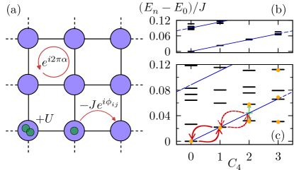
Figure 1: (a) Scheme of the model under consideration. (b-c) Numerically calculated spectrum of the many-body eigenstates for $N=4$ atoms with $\alpha=0.15$ in a (b) $12\times 12$ and (c) $10\times 10$ square lattice (black horizontal lines). In panel (b) the confinement is dominated by a harmonic potential $V_{h}(\mathbf{r})=\omega_{h}^{2}\,(\mathbf{r}-\mathbf{r}_{0})^{2}/2$ of strength $\omega_{h}=0.14J$ around the lattice center $\mathbf{r}_{0}$. In panel (c), the only trapping comes from the open boundaries. Comparison with the linear dispersion of a $\chi$LL theory (blue dashed line) highlights the stronger anharmonicity of the open boundary case of (c): here, the nonlinearity-induced splitting of the $l=2$ manifold is indicated by the green arrows, while the blockade effect is illustrated by the red full/dashed arrows indicating the resonant/detuned transitions. Orange points show the eigenenergies obtained from the diagonalization of the nonlinear $\chi$LL Hamiltonian Eq. (2). The effective parameters $\Omega,\Gamma$ are estimated from the energy of the first excited state and the splitting between the two second excited states, respectively.

We consider the set-up sketched in Fig. 1(a), namely a system of $N$ bosonic particles moving in a $M\times M$ two-dimensional square lattice with open boundaries and lattice spacing $a$, pierced by a uniform and orthogonal (synthetic) magnetic field $B$. We describe the system with the Hofstadter-Bose-Hubbard Hamiltonian [53, 54, 55, 56]

$$\hat{H}_{\text{HBH}}=-J\sum_{\braket{ij}}\left(e^{i\phi_{ij}}\hat{a}_{j}^{{\dagger}}\hat{a}^{{\vphantom{\dagger}}}_{i}+{\rm h.c.}\right)+\frac{U}{2}\sum_{i}\hat{a}_{i}^{{\dagger}}\hat{a}_{i}^{{\dagger}}\hat{a}^{{\vphantom{\dagger}}}_{i}\hat{a}^{{\vphantom{\dagger}}}_{i}$$ (1)

where $\hat{a}^{\vphantom{\dagger}}_{i}$ ($\hat{a}^{\dagger}_{i})$ are the destruction (creation) operators for a particle at site $i$. Both the on-site interaction energy $U$ and the hopping strength $J>0$ are taken uniform in the lattice, and we restrict to the $U\gg J$ hard-core limit. The hopping phase $\phi_{ij}$ from site $i$ to $j$ is related to the magnetic vector potential through $\phi_{ij}=\frac{q}{\hbar}\int_{\mathbf{r}_{i}}^{\mathbf{r}_{j}}\mathbf{A}\cdot d\mathbf{r}$ [57] and gives a gauge-invariant phase $\alpha=2\pi\phi/\phi_{0}$ for hopping around a plaquette. Here, $\phi=Ba^{2}$ is the magnetic flux piercing a plaquette and $\phi_{0}=h/q$ is the flux quantum. Calculations for the eigenstates, the matrix elements, and the dynamics in response to external perturbations are numerically performed by exact diagonalization methods.

This model is known to host a variety of FQH states [55, 58, 59, 60, 61]. In this Letter, we will focus on the simplest Laughlin $\nu=1/2$-like [3] state that correspond to the ground state in the region $0.1\lesssim\alpha\lesssim 0.2$ (see the transparency window in Fig. 2(a-d) [62]). The finite extension of the FQH region is allowed by the flexibility in the value of the density at the center offered by the density-depleted region at the boundary [56, 36, 63, 62].

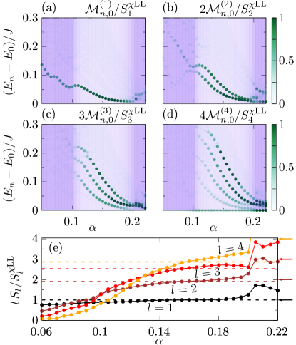
Figure 2: Magnetic field dependence of the excited state eigenenergies in the different $l=1,\ldots,4$ (a-d) sectors. Points are coloured according to the normalized matrix element $l\mathcal{M}_{n,0}^{(l)}/S_{l}$. The purple background transparency is proportional to the overlap of the ground state with a discretized Laughlin state [62]: minimal purple opacity represents maximal overlap.(e) Normalized static structure factor (full lines) compared to the $\chi$LL prediction in the thermodynamic limit (lateral arrows) and a finite-size calculation for a $N=4$ system in the continuum (horizontal dashed lines). Same parameters as in Fig. 1(c).

Nonlinear chiral Luttinger liquid —

In the angular momentum basis labeled by the angular momentum $l>0$, the effective one-dimensional nonlinear $\chi$LL  theory [64, 65, 44] of the edge dynamics of a anharmonically trapped FQH fluid has the form

$$\hat{H}=\!\sum_{l>0}\Omega\,l\,\hat{b}_{l}^{\dagger}\hat{b}_{l}^{\vphantom{\dagger}}\,+\!\sum_{l,l^{\prime}>0}\Gamma\sqrt{ll^{\prime}(l+l^{\prime})}\left[\hat{b}_{l+l^{\prime}}^{\dagger}\hat{b}_{l}^{\vphantom{\dagger}}\hat{b}_{l^{\prime}}^{\vphantom{\dagger}}\!+\!\textrm{h.c.}\right]$$ (2)

where $\hat{b}_{l}$ ($\hat{b}_{l}^{\dagger}$) are the bosonic destruction (creation) operators of Luttinger quanta in the $l$ mode. The first term describes the chiral angular velocity $\Omega$ of edge excitations, as determined by the spatial confinement. On top of this, the anharmonicity of the confinement gives the second term describing scattering processes between Luttinger quanta mediated by a nonlinear term of strength $\Gamma\geq 0$ [44]. Higher-order contributions to the phonon dispersion can be safely neglected as they are irrelevant for the low-energy processes considered in this work [44, 45].

If the trapping is purely harmonic ($\Gamma=0$), the theory reduces to the standard chiral Luttinger liquid [66], where the excitations are non-interacting and have a perfectly linear dispersion. As such, the eigenstates collapse on the $\omega_{l}=\Omega l$ line [blue line in Fig.1(b,c)] and, at each $l$, have a high degeneracy given by the number $P_{l}$ of inequivalent integer partitions of $l$ [10], that is $P_{1}=1,\,P_{2}=2,\,P_{3}=3,\,P_{4}=5,\,\ldots$. Under a generic confinement potential, the massive degeneracy of the eigenstates at a given $l$ is lifted by the nonlinearity in (2).

Spectrum of edge excitations —

In a square lattice the full rotational symmetry is not present; a proper choice of the gauge $\phi_{ij}$ [38] ensures that the discrete rotation operator $e^{i\hat{L}_{z}\frac{\pi}{4}}$ commutes with the system’s Hamiltonian Eq. (1), so that the angular momentum is conserved modulo $4$. Examples of numerically computed excited state spectra are plotted in Fig. 1(b,c) as a function of the reduced angular momentum $C_{4}$. The reduced rotation symmetry makes the $C_{4}$-dependent spectrum to get folded with a period $4$. In Fig. 1(b) the trapping is dominated by an additional harmonic confinement, so that the spectrum is almost linear and resembles the standard $\chi$LL prediction (blue dashed line) with minor splittings and corrections due to the residual anharmonicity. In Fig. 1(c), the only confinement is the one due to the open boundaries: its intrinsic anharmonicity is responsible for marked nonlinear effects and the wide splitting of the multiplets at given $l$. The numerical eigenenergies are in remarkable quantitative agreement with those of the nonlinear $\chi$LL theory Eq. (2), which is is equivalent to a free fermionic theory [45].

This physics is specially visible in the simplest $l=2$ manifold. From the form of (2), it is immediate to recognize that the effect of the nonlinearity is to coherently convert a pair of $l=1$ Luttinger quanta into a single $l=2$ Luttinger quantum and viceversa, so that the eigenstates are non-classical superpositions of the $\hat{b}_{2}^{\dagger}|0\rangle$ and $(\hat{b}_{1}^{\dagger})^{2}|0\rangle$ Fock states above the ground state $|0\rangle$. In analogy with the biexciton Feshbach blockade effect proposed in the optical context in [67], the anharmonicity of the resulting spectrum leads to a marked blockade effect indicated by the red arrows in the level scheme of Fig. 1(c): an external excitation that is resonant with the $l=1$ mode at linear regime will not be able to inject a second quantum, as the corresponding eigenstates are shifted away in energy. A similar analysis holds for the higher $l\geq 3$ multiplets, yet is made less straightforward by the intertwining of the edge-modes splittings with bulk modes, and is further complicated by the folding effect.

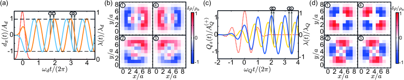
Figure 3: (a) Time evolution of the dipole moment $d_{x}(t)$ (blue solid line) and $d_{y}(t)$ (orange solid line). The pulsed excitation temporal profile $\lambda(t)$ is shown as a red dotted line. (b) Snapshots of the normalized density variation $\delta\rho/\rho_{\rm n}$ at the different time instants indicated in (a). We used $N=3$, $M=9$, $\alpha=0.15$, $\lambda_{d}=10^{-4}J/a$, $\tau J/\hbar=50$ and $\rho_{\rm n}=4\lambda_{d}/(aJ)$. The dipole frequency is $\hbar\omega_{d}/J\approx 0.027$. (c) Time evolution of the real ${\rm Re}[Q_{z}(t)]$ (yellow solid line) and imaginary ${\rm Im}[Q_{z}(t)]$ (blue solid line) parts of the quadrupole moment. The pulsed excitation temporal profile $\lambda(t)$ is shown as a red dotted line. (d) Snapshots of the normalized density variation $\delta\rho/\rho_{\rm n}$ at the different time instants indicated in (c). We used $N=3$, $M=9$, $\alpha=0.15$, $\lambda_{Q}=10^{-5}J/a^{2}$, $\tau J/\hbar=160$ and $\rho_{\rm n}=50\lambda_{Q}/(a^{2}J)$. The quadrupole frequency is $\hbar\omega_{Q}/J\approx 0.035$.

Linear response —

We now proceed with a study of the response of the fluid to external perturbations, starting from the linear regime of a weak excitation. We consider an external potential of angular momentum $l$ and amplitude $\lambda(t)$ of the form $\hat{U}(t)=\sum_{i}U(\mathbf{r}_{i},t)\hat{a}_{i}^{\dagger}\hat{a}_{i}$ with $U(\mathbf{r},t)=\text{Re}\left[z^{l}\lambda(t)\right]$ in terms of the shorthand $z=x+iy$. Beyond their straightforward realization in synthetic matter systems  [68, 44, 40], such potentials can nowadays be implemented also for neutral edge excitations in electronic FQH systems [69]. As a consequence of the transverse Hall response, the component of the force oriented along the azimuthal direction will induce a flow in the radial direction and, thus, a spatially periodic modulation of the density along the edge. Within the $\chi$LL theory [10, 44], the strength of this response is expected to be proportional to the quantized transverse conductivity and thus to the filling factor $\nu$ [62].

Each excited state $\ket{C_{4},n}$ (i.e. the $n$-th excited state at angular momentum $C_{4}$) will give a peak in the response to the external potential located at frequency $\hbar\omega_{C_{4},n}=E_{C_{4},n}-E_{0,0}$ ($E_{0,0}$ being the ground-state energy) with a strength determined by the matrix element $\mathcal{M}_{n,0}^{(l)}=\left|\Braket{C_{4},n\left missing}{\sum\nolimits_{i}z_{i}^{l}\hat{n}_{i}}{0,0}\right|^{2}$ with $C_{4}=l\pmod{4}$. The frequencies and the strengths of the peaks for the lowest $l=1\ldots 4$ excitation channels are summarized in Fig. 2(a-d). In spite of the reduced rotational symmetry, the matrix element weight is concentrated in those eigenstates that result from the splitting of the corresponding multiplet at $l$ in the nonlinear $\chi$LL theory and, as first remarked in [40], excitations to eigenstates folded by Bragg scattering processes have a negligible matrix element. Moreover, the fact that the number of visible $l=4$ states does not match the number of partitions $P_{l=4}=5$ confirms the presence of uncoupled dark edge eigenstates [62] first predicted by the fermionized theory of [45] and here numerically highlighted also in the lattice geometry.

Summing over all the low-energy eigenstates at a given $C_{4}=l\pmod{4}$ that are illustrated in Fig. 2(a-d) provides the numerical value for the structure factor of the edge dynamics $S_{l}=\sum_{n}\mathcal{M}_{n,0}^{(l)}$ that we display in Fig. 2(e). Here, the exact diagonalization results for the lattice geometry (full circles) are compared to the numerical ones for a $N=4$ Laughlin state in a continuum geometry [44] (horizontal dashed lines) [62] and to the $\chi$LL prediction in the thermodynamic limit $S^{\chi LL}_{l}=\nu lR_{\text{cl}}^{2l}$ (lateral arrows). In this last expression, the classical radius $R_{\text{cl}}=\sqrt{2N/\nu}\,l_{B}$ of the FQH cloud accounts for the chosen $r^{l}$ radial dependence of the applied potential and $l_{B}=a/\sqrt{2\pi\alpha}$ is the usual magnetic length.

For sufficiently small $l$, a clear plateau is visible in the region around $\alpha\sim 0.15$ of good overlap with the discrete Laughlin state highlighted in Fig.2(a-d). The height of the plateaus relative to the $l=1$ and $l=2$ modes are in perfect quantitative agreement with the $\chi$LL prediction. For $l>2$ the corrections due to the small number of particles induce sizeable deviations between the $N=4$ lattice numerics and $\chi$LL predictions, while still remaining in quantitative agreement with numerical results for a $N=4$ Laughlin state [62]. This suggests that the observed deviations for the higher multipole excitations are not a consequence of the lattice discretization but of the small particle number.

Measuring the transverse conductivity —

These numerical results provide evidence of the validity of the $\chi$LL theory also in small lattice FQH fluids and suggest that the quantization of the transverse conductivity can be experimentally assessed from a measurement of the response of the fluid to external potentials. Fig. 3(a) illustrate this idea for the $l=1$ dipole case. The single dipole mode can be efficiently excited by means of a spatially uniform and temporally pulsed force, $U(\mathbf{r},t)=\lambda(t)x$ with $\lambda(t)=\lambda_{d}\exp\left[-(t/\tau)^{2}\right]$. A few snapshots of the spatial profile of the density perturbation generated in the fluid at different times are shown in Fig. 3(b). After the end of the perturbation, the $x,y$ components of the dipole moment [blue and yellow lines in Fig. 3(a)] keep oscillating in quadrature at the natural frequency $\hbar\omega_{d}=E_{1,0}-E_{0,0}$ according to $d_{x}(t)=\Braket{\sum\nolimits_{i}x_{i}\hat{n}_{i}}(t)\simeq-A_{d}\sin\left(\omega_{d}t\right)$ and a corresponding formula for $y$. The amplitude $A_{d}=\frac{S_{1}}{2\hbar}\,\widetilde{\lambda}(\omega_{d})$ is the same for the $x,y$ components, proportional to $S_{1}$ and the Fourier component at $\omega_{d}$ of the excitation pulse. From a measurement of $d_{x}(t)$, it is then possible to estimate the structure factor $S_{1}$ and thus the transverse conductivity.

Application of a similar protocol to the higher $l>1$ modes requires isolating the several eigenstates forming the higher multiplets. The quadrupole $l=2$ case is illustrated in Fig.3(c). The two excited states can be separately addressed using a rotating saddle-shaped pulse of the form $U(\mathbf{r},t)=\lambda_{Q}\,\text{Re}\left[z^{2}\lambda(t)\right]$ with a long oscillating pulse $\lambda(t)=e^{-(t/\tau)^{2}}\,e^{-i\omega t}$ [red dotted line in Fig. 3(c)] on resonance with each natural oscillation frequency $\hbar\omega_{Q}=E_{2,0(/1)}-E_{0,0}$. At the end of the excitation pulse, the complex-valued quadrupole moment $Q_{z}(t)=\braket{\sum_{i}(x_{i}^{2}-y_{i}^{2})\hat{n}_{i}}+i\braket{\sum_{i}(2x_{i}y_{i})\hat{n}_{i}}$ keeps oscillating at the selected bare frequency $\omega_{Q}$ as $Q_{z}(t)\simeq A_{Q}^{(+)}e^{i\omega_{Q}t}+A_{Q}^{(-)}e^{-i\omega_{Q}t}$. Here, the counter-rotating terms proportional to $A_{Q}^{(-)}$ stem from the reduced four-fold rotational symmetry of the lattice which enhances (reduces) the quadrupole moment when the density perturbation is along the cartesian (diagonal) directions [Fig. 3(d)]. $A_{Q}^{(+)}$ can be extracted from the amplitude of the real and imaginary parts of $Q_{z}(t)$ and gives direct information on the matrix element $\mathcal{M}_{n,0}^{(2)}=(A_{Q}^{(+)}/\lambda_{Q})(2\hbar/(\sqrt{\pi}\tau))$. Upon summing over both quadrupole modes, the static factor $S_{2}$ provides an estimate of the transverse conductivity, to be compared to the quantized value expected from $\chi$LL theory, Fig. 2(e).

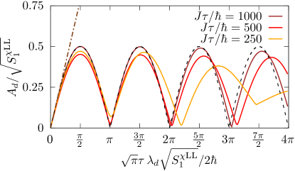
Figure 4: Amplitude of the dipole oscillations under the effect of a monochromatic excitation of different durations $\tau$ as indicated in the legend (solid red, brown, yellow lines) as a function of the (normalized) excitation strength $\lambda_{d}$. Dashed black line shows the theoretical form (3) of the Rabi oscillations. Same parameters as in Fig. 3.

The brown dotted line is the linear regime prediction.

Quantum nonlinear dynamics —

The $\chi$LL theory becomes even richer when one goes beyond the linear response regime and considers excitations that are strong enough to induce nonlinear effects. These are mediated by the new interaction terms that appear in the Hamiltonian Eq. (2) as a consequence of the anharmonic trapping potential. As a simple yet most illustrative example, we consider a quantum blockade effect for edge modes. Let us consider a periodically oscillating potential $U(\mathbf{r},t)=\lambda(t)\cos(\omega_{d}t)x$, resonant with the dipole transition at frequency $\omega_{d}$, with a Gaussian envelope of duration $\tau$ and sizable peak amplitude $\lambda_{d}$. Given the strong anharmonicity of the excitation spectrum highlighted in Fig.1(c), this perturbation is able to efficiently excite the $l=1$ excited state but remains well detuned from all two-excitation states in the higher $l=2$ manifold which therefore remain empty. As a consequence, the dynamics recovers the one of a resonantly-driven two-level system as first noticed in [40], yet with the key advantage of the much stronger nonlinearity due to open boundaries. At the end of the excitation sequence, each dipole component $d_{x,y}$ oscillates at the fast frequency $\omega_{d}$, with an amplitude $A_{d}$. This is determined by the coherent transfer between the ground- and excited- state during the excitation sequence [70], at a Rabi frequency roughly proportional to the perturbation strength $\lambda_{d}$. As one can see in Fig. 4, the Rabi oscillations are cleanest and closest to the theoretical prediction

$$A_{d}=\frac{\sqrt{S_{1}}}{2}\sin\left(\sqrt{\pi}\tau\,\frac{\lambda_{d}\sqrt{S_{1}}}{2\hbar}\right)$$ (3)

for longer-excitation times $\tau$, when the narrower spectrum of the excitation pulse makes the blockade effect on the $l=2$ manifold more effective. As typical in cavity quantum optics, a small system size is beneficial to the blockade effect, as it makes the dynamics faster by reinforcing the nonlinear splitting, and thus helps taming decoherence effects. Interestingly, the dependence of the Rabi oscillation frequency in Eq. (3) on the structure factor offers an alternative way to assess the quantized transverse conductivity of the FQH fluid.

Looking closer at the quantum state generated by the excitation sequence, we note that after a $2\pi$ (or multiple) pulse, the system is brought back to the ground state by the Rabi oscillation, while after a $\pi$ pulse the system is instead fully transferred in its $l=1$ excited state. In a quantum optical language [71] this corresponds to the generation of a very non-classical Fock state with a single Luttinger quantum of excitation in the FQH edge, analogous to a single photon wavepacket in quantum optics. As another remarkable quantum effect, the spectral splitting of the $l=2$ response due to the nonlinear interaction terms of the $\chi$LL theory can be used to convert an $l=2$ Luttinger quantum into a pair of $l=1$ quanta so to obtain a source of correlated Luttinger pairs for quantum optical experiments on FQH edge modes.

Conclusions —

In this work we have shown that the edge dynamics of small lattice fractional quantum Hall fluids [29, 32] is well captured by a nonlinear generalization of chiral Luttinger liquid theory [65, 44]. The response to time-dependent external potentials carries evidence of a quantized value of the transverse conductivity in the bulk. Turning the small spatial size and the open boundaries of state-of-the-art systems [31, 29, 32, 30] into an advantage, we have moved the first steps into quantum nonlinear optics of FQH edge modes: thanks to the intrinsic nonlinearity stemming from spatial confinement, quantum blockade effects set in and lead to the generation of nonclassical states of the edge modes. Future theoretical work will deal with more complex quantum optical effects, such as the generation of entangled $\chi$LL pairs [72], solitonic and bunched excitations of the fractional quantum Hall edge [73, 74, 75] and exploitation of the edge as a information channel between localized impurities [76, 77].

Acknowledgements —

We are thankful to E. Macaluso for continuous collaboration in the first ground-breaking steps of this work, N. Goldman, J. Kwan and the M. Greiner group for insightful discussions. A.N. acknowledges financial support from Fondazione Angelo dalla Riccia, LoCoMacro 805252 from the European Research Council and LPTMS for warm hospitality. D.D.B. acknowledges funding from the European Union - NextGeneration EU, ”Integrated infrastructure initiative in Photonic and Quantum Sciences” - I-PHOQS [IR0000016, ID D2B8D520, CUP B53C22001750006]. M.R. acknowledges support from the Deutsche Forschungsgemeinschaft (DFG) via project Grant No. 277101999 within the CRC network TR 183 (B01) and under Germany’s Excellence Strategy – Cluster of Excellence Matter and Light for Quantum Computing (ML4Q) EXC 2004/1 – 390534769. I.C. acknowledges financial support from the European Union H2020-FETFLAG-2018-2020 project “PhoQuS” (n.820392), from the Provincia Autonoma di Trento, from the Q@TN initiative, and from the PNRR MUR project PE0000023-NQSTI. This work is part of HQI initiative (www.hqi.fr) and is supported by France 2030 under the French National Research Agency award number “ANR-22-PNCQ-0002”.

Supplemental Material for
Quantum nonlinear optics on the edge of small lattice fractional quantum Hall fluids

I Wen’s matrix elements

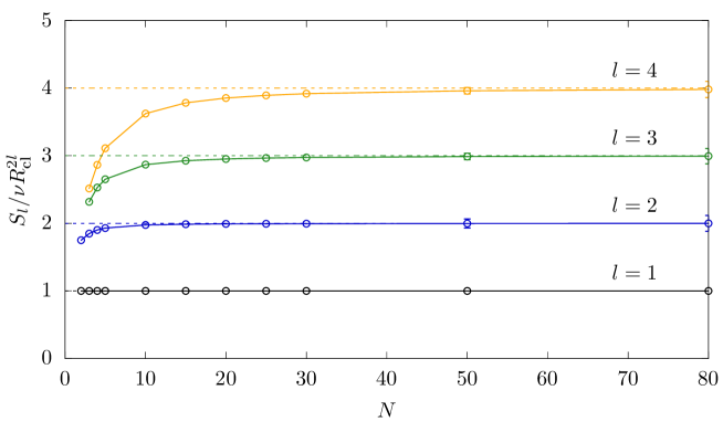
Figure 5: Low-energy static structure factor $S_{l}$ (see Eq. (5)) for a continuum Laughlin state as a function of the number of particles $N$. Our results are normalized to the expected result $S_{l}^{\text{$\chi$LL~{}}}$ (see Eq. (9) per contributing state $l$, $S_{l}^{\text{$\chi$LL~{}}}/l=\nu R_{\text{cl}}^{2l}$. The points are the results of Monte-Carlo simulations, while the dashed lines highlight the expected limit $l$.

In this section we review the theory for the static structure factor of the relevant observable $\sum_{i=1}^{N}z_{i}^{l}$ in the case of a $N$-particle Laughlin state in the continuum, in the thermodynamic limit $(N\gg 1)$. In this case the system is fully rotationally symmetric; the angular momentum is a good quantum number, and we can label the system’s eigenstates as $\ket{l,n}$, with $l$ being the angular momentum with respect to the one of the Laughlin ground state. Here $n$ is the additional quantum number which enumerates the system’s eigenstates at fixed $l$. We are interested in the matrix elements

$$S_{l}=\sum_{n}\left|\Braket{l,n\left missing}{\sum_{i=1}^{N}z_{i}^{l}\,}{0}\right|^{2}.$$ (4)

These matrix elements can be conveniently rewritten as

$$S_{l}=\sum_{n}\left|\int r^{l}e^{il\theta}\Braket{l,n\left missing}{\hat{\rho}(\mathbf{r})}{0}d^{2}\mathbf{r}\right|^{2}.$$ (5)

Since the bulk is incompressible, the only contributions can come from a thin layer at the system’s edge, close to system’s classical radius $R_{\text{cl}}=\sqrt{2N/\nu}l_{B}$, $l_{B}$ being the magnetic length; in the large particle number ($N\gg 1$) limit the previous expression can be approximated by

$$S_{l}\approx R_{\text{cl}}^{2l}\sum_{n}\left|\Braket{l,n\left missing}{\widetilde{\rho}_{l}}{0}\right|^{2}.$$ (6)

where $\widetilde{\rho}_{l}=\int e^{il\theta}\widetilde{\rho}(\theta)d\theta$ is the angular Fourier transform of a one-dimensional effective density $\widetilde{\rho}(\theta)=\int\hat{\rho}(\mathbf{r})rdr$. Following Wen’s bosonization we can replace the full $\widetilde{\rho}_{l}$ operators with bosonic fields

$$\widetilde{\rho}_{l}=\sqrt{\nu l}\,\hat{b}^{\dagger}_{l},$$ (7)

where $\left[\hat{b}_{l}^{\vphantom{\dagger}},\hat{b}_{l^{\prime}}^{\dagger}\right]=\delta_{l,l^{\prime}}$, and see the excited states $\ket{l,n}$ as being generated by the current algebra through

$$\ket{l,n}=\prod_{l^{\prime}\in\boldsymbol{\lambda_{l}}}\frac{b^{\dagger}_{l^{\prime}}}{\sqrt{n_{l^{\prime}}!}}\ket{0}$$ (8)

where $\boldsymbol{\lambda}_{l}$ is an integer partition with angular momentum $l$ and $n_{l^{\prime}}$ the multiplicity with which $l^{\prime}$ appears in $\boldsymbol{\lambda}_{l}$. The only state contributing to the summation in Eq. (6) is therefore $\ket{l,n}=\hat{b}^{\dagger}_{l}\ket{0}$, and we get

$$S_{l}\approx\nu l\,R_{\text{cl}}^{2l}.$$ (9)

Some numerical Monte-Carlo results obtained as detailed in [44, 45] for the edge-excitations on top of a bosonic $\nu=1/2$ state are shown as a function of the number of bosons $N$ for $l=1,\ldots,4$ in Fig. 5.

Notice that at $l=1$ the result is filling-fraction-independent and compatible with Kohn’s theorem, as we will detail in the next section, and the numerical result for a translationally invariant system in Fig. 5 indeed exactly matches the result of Eq. (9); however it should also be noticed that there is no a-priori reason for our lattice system to obey Kohn’s theorem and the result we show for $l=1$ has to be understood as a signature of fractional quantum Hall physics.

II Kohn’s theorem

In this section we briefly review the content of Kohn’s theorem [78]. The system one considers is a collection of $N$ quantum particles moving in two-dimensions under the influence of a perpendicular magnetic field, $B$, under the influence of internal forces alone and at most an external harmonic potential

$$H=\sum_{i=1}^{N}\frac{(\mathbf{p}_{i}-q\mathbf{A}(\mathbf{r}_{i}))^{2}}{2M}+\sum_{i=1}^{N}\frac{1}{2}M\omega^{2}\mathbf{r}_{i}^{2}+\sum_{1\leq i<j\leq N}V(\mathbf{r}_{i}-\mathbf{r}_{j}).$$ (10)

We here use the symmetric gauge, $\mathbf{A}(\mathbf{r})=\frac{B}{2}(-y,x,0)$. The motion of the center of mass can be decoupled from the one of the $N-1$ remaining relative coordinates; the former is ruled by a simple Hamiltonian: introducing the center of mass variable $\mathbf{R}=\frac{1}{N}\sum_{i}\mathbf{r}_{i}$ and its canonically conjugate momentum $\mathbf{P}=\sum_{i}\mathbf{p}_{i}$ one can separate the Hamiltonian $H=H_{\text{rel}}+H_{\text{CM}}$ into two parts, a part $H_{\text{rel}}$ which only depends on the $N-1$ relative coordinates and a second part $H_{\text{CM}}$ which instead depends only on the center of mass coordinates

$$H_{\text{CM}}=\frac{\mathbf{P}^{2}}{2M^{\prime}}-\frac{\omega_{c}}{2}L_{z}+\frac{1}{2}M^{\prime}\Omega^{2}\mathbf{R}^{2},$$ (11)

where $L_{z}=(\mathbf{R}\times\mathbf{P})\cdot\hat{z}$ is the center of mass angular momentum. Here we introduced the cyclotron frequency $\omega_{c}=\frac{qB}{M}$, the total mass $M^{\prime}=NM$ and an effective oscillator frequency $\Omega=\sqrt{\omega^{2}+\omega_{c}^{2}/4}$. The eigenfunctions are those of a harmonic oscillator; introducing radial $R$ and azimuthal $\theta$ coordinates for the center of mass position, these eigenfunctions can be written as

$$\Phi_{n,m}^{(\text{CM})}(R,\theta)=\frac{1}{\sqrt{\pi\frac{\Gamma\left(n+\frac{|m|+m}{2}+1\right)}{\Gamma\left(n-\frac{|m|-m}{2}+1\right)}\,l_{\text{CM}}^{2}}}\,\left(\frac{R}{l_{\text{CM}}}\right)^{|m|}e^{im\theta}\,L_{n-\frac{|m|-m}{2}}^{(|m|)}\left(\frac{R^{2}}{l_{\text{CM}}^{2}}\right)\,e^{-\frac{R^{2}}{2l_{\text{CM}}^{2}}},$$ (12)

where $\Gamma(n)$ is Euler’s Gamma function, $L_{n}^{(\alpha)}(x)$ are associated Laguerre polynomials and we introduced a center of mass unit of length $l_{CM}=\sqrt{\frac{\hbar}{M^{\prime}\Omega}}$. These wavefunctions diagonalize the center of mass angular momentum, $L_{z}\Phi_{n,m}^{(\text{CM})}=m\,\Phi_{n,m}^{(\text{CM})}$, as well as the center of mass Hamiltonian Eq. (11), with eigenvalue

$$E_{n,m}^{(\text{CM})}=\frac{\hbar\Omega}{2}\,\left[4\left(n+\frac{m+1}{2}\right)-\frac{\omega_{c}}{\Omega}\,m\right].$$ (13)

In terms of the principal quantum number $n\in\mathbb{N}$, the angular momentum quantum number $m$ must satisfy $m\geq-n$. For any value of $\omega$, the ground state can be seen to correspond to $n=0$, $m=0$.

When the cyclotron frequency is much larger than the harmonic confinement one, $\omega_{c}\gg\omega$, the energies reduce to Landau level ones $E_{n,m}^{(\text{CM})}\simeq\hbar\omega_{c}\,\left(n+\frac{1}{2}\right)$, independent of the angular momentum quantum number $m$. This center of mass separation is relevant for the evaluation of the matrix elements of certain observables, such a

$$U= \sum_{i}z_{i}=NR\,e^{+i\theta}$$ (14)

$$U^{*}= \sum_{i}z_{i}^{*}=NR\,e^{-i\theta}$$

since they only depend on the center of mass variables and not on the $N-1$ relative coordinates. In particular, $U$ couples the ground state only to $n=0$, $m=1$. This can be seen to be a low-energy excitation, since it does not change the Landau level quantum number $n$. $U^{*}$ on the other hand couples the ground state only to $n=1$, $m=-1$; it therefore represents an high-energy excitation (whose cost is set by the cyclotron energy $\hbar\omega_{c}$). This result is known as the Kohn’s cyclotron’s resonance [78]. It is not difficult to show that

$$\bra{\Phi_{0,1}^{(\text{CM})}}U\ket{\Phi_{0,0}^{(\text{CM})}}=N\,l_{\text{CM}}\xrightarrow[\omega_{c}\gg\omega]{}\sqrt{2N}\,l_{B}$$ (15)

where $l_{B}=\sqrt{\frac{\hbar}{M\omega_{c}}}$. Since this single state is contributing at low-energies (in the limit $\omega_{c}\gg\omega$), we get

$$S_{1}=|\bra{\Phi_{0,1}^{(\text{CM})}}U\ket{\Phi_{0,0}^{(\text{CM})}}|^{2}=2N\,l_{B}^{2},$$ (16)

which is the same result Eq. (9) obtained in the previous section in the case in which the angular momentum carried by $\sum_{i}z_{i}^{l}$ is $l=1$. Notice also that information on the relative motion will start to matter for any $l>1$.

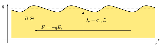
Figure 6: Schematic depiction of a quantum Hall system with an edge. The yellow region represents the incompressible quantum Hall fluid, whose edge (the black curly line) is deformed with respect to its ground-state position (the dashed black line). A force is applied along the $\hat{x}$ direction and a current flows proportionally to the applied force in the $\hat{y}$ direction due to the presence of a strong perpendicular magnetic field.

III $\chi$LL commutation relations

In this section we want to give an alternative heuristic derivation of the commutation relations of the density operators of a $\chi$LL , which highlights the connection with the transverse conductivity of the bulk and does not rely on a specific form for the edge Hamiltonian.

We consider a quantum Hall region infinite in the $\hat{x}$ direction and semi-infinite in the $\hat{y}$ direction, as we schematically depict in Fig. 6. The magnetic field is along the $\hat{z}$ direction. If we apply a constant force in the $\hat{x}$ direction, by imposing an external potential $U=qE_{x}x$, a quantized current flows in the bulk $J_{y}=\sigma_{xy}E_{x}$ perpendicularly to the edge.

Since charge is conserved, a continuity equation $\partial_{t}\rho=-\boldsymbol{\nabla}\cdot\boldsymbol{J}/q$ must hold. For the present discussion, we only focus on the effect of this transverse current and not on the charge dynamics once the edge is reached (i.e. we neglect the chiral motion along the boundary caused by the sample confinement) by dropping the $\hat{x}$ contribution to the current; more explicitly, $\partial_{t}\rho\simeq-\partial_{y}J_{y}/q$. We now integrate this equation along the $\hat{y}$ direction, from the bulk region (where the density has not changed because of the bulk’s incompressibility and $J_{y}^{\text{bulk}}=\sigma_{xy}E_{x}$) to the outside of the sample (where both the density and the current vanish)

$$\frac{\partial}{\partial t}\int dy\rho(x,y)=-\frac{1}{q}\int dy\frac{\partial J_{y}}{\partial y}=\frac{1}{q}J_{y}^{\text{bulk}}=\frac{\sigma_{xy}}{q^{2}}\frac{\partial U}{\partial x}.$$ (17)

On the other hand, the left hand side of the expression can be rewritten by subtracting off the equilibrium density and $\int dy\left[\rho(x,y)-\rho_{0}(y)\right]=\delta\rho(x)$ can be seen as an effective edge density.

From a more microscopic perspective, $U$ couples to the system’s density $\hat{\rho}=\hat{\Psi}^{\dagger}\hat{\Psi}^{\vphantom{\dagger}}$ through an interaction Hamiltonian

$$\hat{H}=\int dx\,dy\,U(x)(\hat{\rho}-\rho_{0})=\int dx\,U(x)\int dy(\hat{\rho}-\rho_{0})=\int dx\,U(x)\delta\hat{\rho},$$ (18)

and Eq. (17) can be seen as the expectation value of a Heisenberg equation of motion $\frac{\partial}{\partial t}\delta\hat{\rho}(x)=\frac{\sigma_{xy}}{q^{2}}\frac{\partial U}{\partial x}$. In order for this to be compatible with the Hamiltonian Eq. (18), we need

$$\frac{i}{\hbar}\left[\hat{H},\delta\hat{\rho}(x)\right]=\frac{\partial}{\partial t}\delta\hat{\rho}(x)=\frac{\sigma_{xy}}{q^{2}}\frac{\partial U}{\partial x},$$ (19)

or

$$\frac{i}{\hbar}\int dy\,U(y)\left[\delta\hat{\rho}(y),\delta\hat{\rho}(x)\right]=\frac{\sigma_{xy}}{q^{2}}\frac{\partial U}{\partial x}.$$ (20)

If we assume $\left[\delta\hat{\rho}(y),\delta\hat{\rho}(x)\right]=\alpha\delta^{\prime}(y-x)$, we get $\alpha=i\frac{\hbar\sigma_{xy}}{q^{2}}$ or

$$\begin{split}\left[\delta\hat{\rho}(y),\delta\hat{\rho}(x)\right]=&i\frac{\sigma_{xy}}{\hbar q^{2}}\delta^{\prime}(y-x)\\ =&i\frac{\nu}{2\pi}\delta^{\prime}(y-x)\end{split}$$ (21)

which indeed does coincide with the famous $\chi$LL liquid commutation relations derived by Wen [6, 7, 8, 11, 10]. This highlights the connection between the non-Fermi-liquid commutator Eq. (21) (which in turn is responsible for the static structure factor value in Eq. (9)) and the bulk’s transverse conductivity.

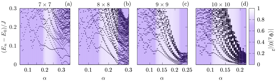
Figure 7: Energy levels $E_{n}$ (with respect to the system’s ground state energy $E_{0}$) as a function of the magnetic flux per plaquette $\alpha$, for $N=4$ hard-core bosons moving in a (a) $7\times 7$, (b) $8\times 8$, (c) $9\times 9$, (d) $10\times 10$ square lattice. The purple background transparency is regulated according to the (squared) overlap of the ground state $\ket{0}$ with the discretized Laughlin state of Eq. (22), $\ket{\Psi_{L}}$. In order for the data point not to disappear when the overlap drops, when the squared overlap drops below $0.7$ the transparency is kept constant.

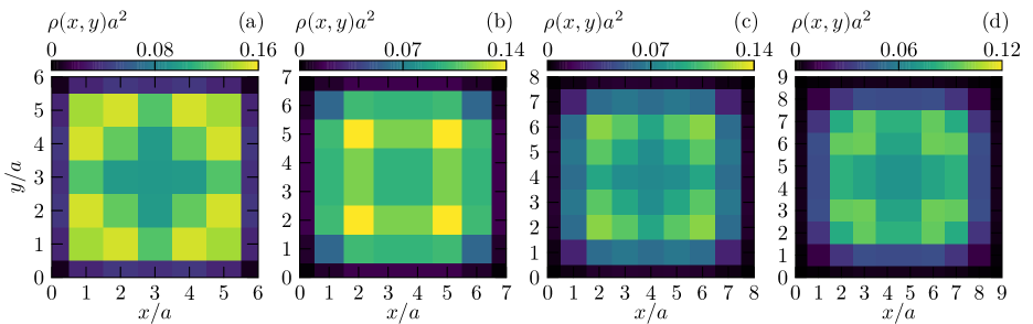
Figure 8: Ground state densities of the $N=4$ hard-core boson system in lattices with different sizes, for some selected values of the magnetic flux per plaquette $\alpha$ which correspond to a ground state in the Laughlin phase. In particular, the four panels correspond to (a) $7\times 7$ lattice with $\alpha=0.22$, (b) $8\times 8$ lattice with $\alpha=0.21$, (c) $9\times 9$ lattice with $\alpha=0.17$ and (d) $10\times 10$ lattice with $\alpha=0.15$. The particular values of $\alpha$ have been chosen so as to (approximately) maximize the overlap (see Fig. 10) of the given state with the discretized Laughlin wavefunction in Eq. (22).

IV Lattice-size effects

In this section we analyze how the number of lattice sites influences the energy spectra and the structure factors.

In Fig. 7 we show the excitation spectra for $N=4$ particles on a $M\times M$ lattice, for $M=7,\ldots,10$. The background transparency is regulated according to the overlap of the ground state with a discretized bosonic Laughlin wavefunction

$$\Psi_{L}=\prod_{1\leq i<j\leq N}(z_{i}-z_{j})^{1/\nu}\,e^{-\frac{1}{4l_{B}^{2}}\sum_{i=1}^{N}|z_{i}|^{2}}.$$ (22)

Here $\nu=1/2$ is the (robust) filling fraction associated to the particular incompressible phase, while $z_{i}=x_{i}+iy_{i}$ take values on the square lattice. A large region in which the ground state has a large overlap with this model-wavefunction can be seen (see also Fig. 10). It can also be seen from Fig. 7 that as the size of the lattice is increased (from the leftmost panel to the rightmost), the edge-excitation velocity decreases, as can be expected from the atoms avoiding the occupation of the boundary lattice sites (see Fig 8).

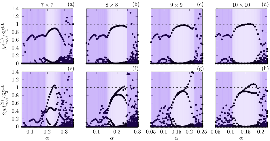
Figure 9: Matrix elements $\mathcal{M}_{n,0}^{(l)}=\left|\Braket{n}{\sum_{i}z_{i}^{l}\hat{n}_{i}}{0}\right|^{2}$ as a function of the magnetic flux per plaquette $\alpha$, for $N=4$ hard-core bosons, moving in a (a,e) $7\times 7$, (b,f) $8\times 8$, (c,g) $9\times 9$, (d,h) $10\times 10$ square lattice. The top (a-d) (/bottom (e-h)) panels are for $l=1$ (/$l=2$). The purple background transparency is regulated according to the (squared) overlap of the ground state $\ket{0}$ with the discretized Laughlin state of Eq. (22), $\ket{\Psi_{L}}$. In order for the data point not to disappear when the overlap drops, when the squared overlap drops below $0.7$ the transparency is kept constant. The static structure factor per state $S_{l}^{\text{$\chi$LL~{}}}/l$ given by Eq. (4) is shown as black dashed lines.

In Fig. 9 we then plot the matrix elements $\mathcal{M}_{n,0}^{(l)}$ for $l=1,2$; since in the Laughlin region only $l$ modes have large matrix-elements, we normalize the results to the integrated structure factor per state in the continuum, $S^{\text{$\chi$LL~{}}}_{l}/l=\nu R_{\text{cl}}^{2l}$, $R_{\text{cl}}=\sqrt{2N/\nu}l_{B}$ being the classical radius and $l_{B}$ the magnetic length. This result can be obtained from a $\chi$LL description of the edge excitations of a Laughlin ground state in the continuum, as we explicitly showed in the first section. With such a normalization, summing over the $l$ non-vanishing matrix elements should therefore give $l$, provided the geometric factor $R_{\text{cl}}^{2l}$ is not strongly affected by the shape of the square boundary. As the system size is increased, it can be seen in Fig. 9(a-d) that the dipole matrix element ($l=1$) does indeed approach the expected result $S^{\text{$\chi$LL~{}}}_{1}=\nu R_{\text{cl}}^{2}$; panels(e-h) show instead what happens for the quadrupole matrix elements: in the Laughlin region (highlighted by the purple transparency) as the number of lattice sites is increased two states only (full circles) contribute to the structure factor $S^{\text{$\chi$LL~{}}}_{2}$; it can also be seen how their magnitude approaches $S^{\text{$\chi$LL~{}}}_{2}/2=\nu R_{\text{cl}}^{4}$, hinting to the correctness of the sum rule Eq. (6). We will show in greater detail in the next section (in particular in Fig. 12) how $S^{\text{$\chi$LL~{}}}_{2}$ changes as a function of the magnetic flux per plaquette $\alpha$, for various lattice sizes and number of particles.

Finally, in Fig. 10 we plot the overlaps of a few selected eigenstates with discretized model fractional quantum Hall wavefunctions for the gapless edge excitations of a Laughlin liquid, for different system sizes. In particular, the ground state, with symmetry eigenvalue $C_{4}$, which we label $\ket{C_{4},0}$, is compared to the discretized Laughlin wavefunction of Eq. (22); a good agreement (black curves) for the squared overlaps ($|\Braket{\Psi_{L}}{C_{4},0}|^{2}$ up to $\sim 0.9$) can be seen over a wide range of synthetic magnetic flux per plaquette $\alpha$, for various lattice sizes. The lowest lying excitation $\ket{C_{4}^{\prime},0}$, where $C_{4}^{\prime}=C_{4}+1\pmod{4}$, is compared instead to the edge excitation

$$\Psi_{d}=\sum_{i}z_{i}\prod_{1\leq i<j\leq N}(z_{i}-z_{j})^{1/\nu}\,e^{-\frac{1}{4l_{B}^{2}}\sum_{i=1}^{N}|z_{i}|^{2}}.$$ (23)

Again, a good agreement (red curves) can be found in the same region of $\alpha$, although this window is slightly narrower.

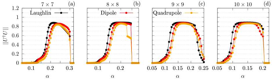
Figure 10: Overlaps between selected numerical eigenstates and model fractional quantum Hall wavefunctions for the Laughlin state Eq. 22 and its edge excitations Eq. (23), Eq. (24), for a $N=4$ system of hard-core bosons moving on (a) $7\times 7$, (b) $8\times 8$, (c) $9\times 9$ and (d) $10\times 10$ lattices, as a function of the synthetic magnetic flux per plaquette.

Finally, the two quadrupolar modes $\ket{C_{4}^{\prime\prime},0}$ and $\ket{C_{4}^{\prime\prime},1}$ can be compared to discretized quadrupolar excitations of a Laughlin state

$$\begin{split}\Psi_{q}&=\left(\sum_{i}z_{i}\right)^{2}\prod_{1\leq i<j\leq N}(z_{i}-z_{j})^{1/\nu}\,e^{-\frac{1}{4l_{B}^{2}}\sum_{i=1}^{N}|z_{i}|^{2}}\\ \Psi_{q}^{\prime}&=\sum_{i}z_{i}^{2}\prod_{1\leq i<j\leq N}(z_{i}-z_{j})^{1/\nu}\,e^{-\frac{1}{4l_{B}^{2}}\sum_{i=1}^{N}|z_{i}|^{2}}.\end{split}$$ (24)

These two states $\ket{\Psi_{q}}$ and $\ket{\Psi_{q}^{\prime}}$ are linearly independent but not orthonormal: we therefore orthonormalize them with a standard Gram-Schmidt procedure; moreover, it does not make sense to compare the two separately to the two quadrupolar states $\ket{C_{4}^{\prime\prime},0}$ and $\ket{C_{4}^{\prime\prime},1}$: in principle we can however expect these to be a mixture of $\ket{\Psi_{q}}$ and $\ket{\Psi_{q}^{\prime}}$ which minimizes the particular Hamiltonian, provided mixing with states outside of this manifold is small. We test this idea by defining a matrix of overlaps

$$U=\begin{pmatrix}\braket{\Psi_{q}}{C_{4}^{\prime\prime},0}&\braket{\Psi_{q}^{\prime}}{C_{4}^{\prime\prime},0}\\ \braket{\Psi_{q}}{C_{4}^{\prime\prime},1}&\braket{\Psi_{q}^{\prime}}{C_{4}^{\prime\prime},1}\end{pmatrix}$$ (25)

and testing whether it defines an unitary matrix (i.e. a “rotation” between two otherwise equivalent bases) by computing an Hilbert-Schmidt norm of $U^{\dagger}U^{\vphantom{\dagger}}$

$$||U^{\dagger}U^{\vphantom{\dagger}}||=\sqrt{\frac{1}{d}\sum_{i,j=1}^{d}\left|(U^{\dagger}U^{\vphantom{\dagger}})_{i,j}\right|^{2}},$$ (26)

where $d$ is the dimension of the subspace under consideration; in this case, $d=2$. Ideally, $U^{\dagger}U^{\vphantom{\dagger}}=\mathbb{1}$ and the normalization in Eq. (26) has been chosen so that $||\mathbb{1}||=1$. Notice finally that when $d=1$, Eq. (26) reduces to the squared overlap used in the two previous cases with the ground- and dipole- states. Again, a good agreement (yellow curve) can be seen in the relevant region of $\alpha$ in Fig. 10, with $||U^{\dagger}U^{\vphantom{\dagger}}||\approx 0.9$.

Although these overlaps can be expected to drop to zero in the thermodynamic limit  ($N,L\rightarrow\infty$), the fact that they are significantly close to $1$ in a limited window of fluxes per plaquette for the lattice sizes we analysed supports our interpretation of them being the edge modes of a Laughlin state. Let us finally stress that the fact that we expect these overlaps to drop does not mean that our conclusions will be altered: on the contrary, Eq. (6) is a thermodynamic limit statement and a consequence of dealing with a Laughlin topological order , and not of exactly having model Laughlin-like wavefunctions for the ground state and its excitation.

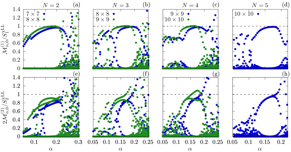
Figure 11: Matrix elements $\mathcal{M}_{n,0}^{(l)}=\left|\Braket{n}{\sum_{i}z_{i}^{l}\hat{n}_{i}}{0}\right|^{2}$ as a function of the magnetic flux per plaquette $\alpha$, for (a,e) $N=2$ (b,f) $N=3$, (c,g) $N=4$ and (d,h) $N=5$ hard-core bosons, for different lattice sizes. The top (a-d) (/bottom (e-h)) panels are for $l=1$ (/$l=2$). The static structure factor per state $S_{l}^{\text{$\chi$LL~{}}}/l$ given by Eq. (4) is shown as black dashed lines.

V Scaling with the number of particles

In this section we briefly show and discuss the results for the matrix elements $\mathcal{M}_{n,0}^{(l)}$ for different number of particles.

In particular, in Fig. 11 the results in the $l=1,2$ cases are shown as a function of the synthetic magnetic flux per plaquette $\alpha$, for different lattice sizes. In the top panels (a-d) we show the results for $\mathcal{M}_{n,0}^{(1)}$. It can be seen that a single state has a significantly non-zero matrix element in the region of $\alpha$ in which the ground state is a Laughlin state. Only this state, which we identify with the dipole excitation of Eq. (23), contributes to the integrated structure factor of Eq. (4); indeed it can be seen that in the Laughlin region the value of this matrix element collapses to the static structure factor curve Eq. (9) (black dashed line), for every $N$ and $L$ displayed here.

In the bottom panels (e-h) we instead show the results for $\mathcal{M}_{n,0}^{(2)}$. It can be seen that only two states contribute significantly to the static structure factor Eq. (4); we interpret these two states as the quadrupole modes of a Laughlin state, Eq. (24). The matrix elements have been compared to the expected static structure factor per state, $S_{l}^{\text{$\chi$LL~{}}}/l$ (black dashed line); as we already discussed in the previous section, it is important to notice that there is no a priori reason why the two matrix elements should be equally contributing to $S_{l}^{\text{$\chi$LL~{}}}$: in principle only one of them could be carrying all the spectral weight (see for example Eq. (6), Eq. (7) and Eq. (8) above). It can however be seen, at least qualitatively, that as the number of particles is increased, the expected value of $S_{l}^{\text{$\chi$LL~{}}}$ is reached.

We also performed a more quantitative test. In particular, in Fig. 12 we show the integrated dynamic structure factor, namely $S_{l}=\sum_{n}\mathcal{M}_{n,0}^{(l)}$. In the $l=1$ case (panels (a-d)) a good agreement with the prediction for $S_{l}^{\text{$\chi$LL~{}}}$ given by Wen’s theory (black dashed line), Eq. (9), can be seen. In the $l=2$ case (panels e-h)), even though the integrated structure factor $S_{l}$ deviates from this prediction, as the number of particles is increased the plateau that $S_{l}$ exhibits gets closer to $S_{l}^{\text{$\chi$LL~{}}}$. Furthermore, this finite size correction is compatible with the results (red dotted dashed line) that we obtained for a Laughlin state in the continuum (see Fig. 5).

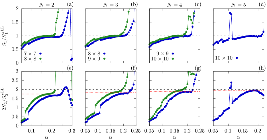
Figure 12: Static structure factors $S_{l}=\sum_{n}\mathcal{M}_{n,0}^{(l)}$ as a function of the magnetic flux per plaquette $\alpha$, normalized to the static structure factor per contributing state $S_{l}^{\text{$\chi$LL~{}}}/l$ given by Eq. (9); in the various panels, different system sizes are shown: (a,e) $N=2$ (b,f) $N=3$, (c,g) $N=4$ and (d,h) $N=5$. The expected static structure factor given by Eq. (9) is shown as black dashed lines. The top (a-d) (/bottom (e-h)) panels are for $l=1$ (/$l=2$). In the $l=2$ cases (panels (e-h)), the red dashed-dotted lines are the results for the static structure factor Eq. (5) for a continuum state (see also Fig. 5).

VI Effect of additional harmonic confinement

In this section we analyse the effect of an additional harmonic confinement which does not spoil the fourfold rotational symmetry of the lattice; namely, we add to the Harper-Hofstadter Hamiltonian an additional potential term

$$\hat{U}_{\text{conf}}=\sum_{i,j}U_{\text{h}}a^{2}\left(\left(i-\frac{M-1}{2}\right)^{2}+\left(j-\frac{M-1}{2}\right)^{2}\right)\hat{n}_{ij}.$$ (27)

We study the energies and matrix elements $\mathcal{M}_{n,0}^{(l)}$ as a function of $U_{\text{h}}$ in Fig. 13.

In the absence of the harmonic confinement, when plotted against the fourfold discrete rotation symmetry eigenvalue $C_{4}$, the level structure cannot be easily interpreted visually (see Fig. 13(a)) due to the competing energy-scales of bulk and edge excitations. However, a weak harmonic confinement isolates in each symmetry sector a low-lying group of states with the counting predicted by the edge-mode theory for a Laughlin state (see Fig. 13(f)). The degeneracy is slightly shifted by perturbations of Wen’s Hamiltonian, leading to a weakly non-linear $\chi$LL  [65, 44, 45].

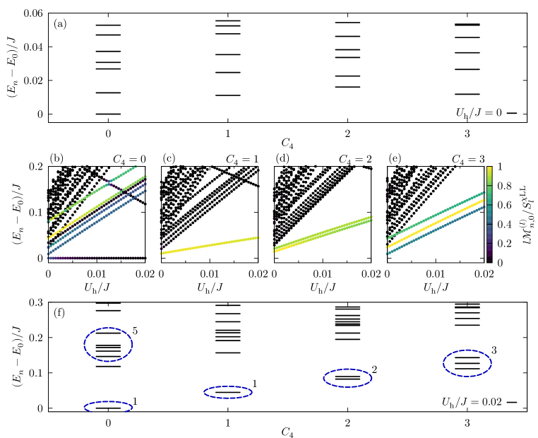
Figure 13: (a) Energy levels (with respect to the ground state one) of a system of $N=4$ hard-core bosons moving on a $10\times 10$ lattice, at $\alpha=0.18$. The energies are plotted against the fourfold discrete rotation symmetry eigenvalue $C_{4}$.
(b-e) Energy levels (with respect to the ground state one) for the same system, as a function of the harmonic confinement strength $U_{\text{h}}$ (see Eq. (27); the various panels refer to the different $C_{4}$ values: (b) $C_{4}=0$ (c) $C_{4}=1$ (d) $C_{4}=2$ and (e) $C_{4}=3$. The points are coloured according to the value of the matrix elements $\mathcal{M}_{n,0}^{(l)}=\left|\braket{n\left missing}{\sum_{i}z_{i}^{l}\hat{n}_{i}}{0}\right|^{2}$, for $l=C_{4}\pmod{4}$, i.e. (b) $l=4$, (c) $l=1$, (d) $l=2$ and (e) $l=3$.
(f) Energy levels (with respect to the ground state one) plotted against the symmetry eigenvalue $C_{4}$ for the same system, in the presence of an additional harmonic confinement with strength $U_{h}/J=0.02$. Dashed-blue ellipses highlight the now well isolated group of edge modes with the counting predicted for a Laughlin ground state [38, 40].

In the mid panels, Fig. 13(b-e), we show that the ground state in the absence of the harmonic confinement Eq. (27) is adiabatically connected to the ground state in its presence, which is unambigously identified to be a Laughlin topological order by the edge-mode counting seen in Fig. 13(f). Furthermore, the lowest lying states at $l=1$ and $l=2$ can be seen to be connected with the low-lying edge excitations highlighted in Fig. 13(f). This supports the results we previously exhibited in Fig. 10 for the overlaps with the discretized model wavefunctions for the Laughlin state of Eq. (22) and its edge excitations Eq. (23) and Eq. (24).

The points in Fig. 13(b-e) are also coloured according to the matrix elements $\mathcal{M}_{n,0}^{(l)}=\left|\braket{n\left missing}{\sum_{i}z_{i}^{l}\hat{n}_{i}}{0}\right|^{2}$; it is worth highlighting some features. First of all in the $C_{4}=3$ plot in Fig. 13 (panel (e)) it can be seen that the $3$ states that carry non-zero weight for the $l=3$ excitation are those that at large $U_{\text{h}}$ can be identified with the $3$ edge excitations of a continuum Laughlin liquid at the same angular momentum variation with respect to the ground state; at small $U_{\text{h}}$ these states cross with other levels, but they do not mix with them. Secondly, for $N=4$ particles, also the counting of edge modes in the $C_{4}=4\equiv 0\pmod{4}$ symmetry sector shown Fig. 13(b) is expected to show the thermodynamic-limit counting [10, 80] (i.e. a group of $5$ states). For the parameters we used however this is not so clear. Indeed in Fig. 13(b) it can be seen that around $U_{\text{h}}/J=0.01$ there is a low-lying group of $5$ states which couple to the density operator in the same way a non-harmonically confined Laughlin state does [44, 45] - namely only $4$ states couple to it while the fifth one is dark; however, as $U_{\text{h}}$ is further increased there is a level crossing (for which we lack an intuitive understanding) at around $U_{\text{h}}/J\approx 0.12$, mixing in this subspace. This makes the interpretation of the low-lying group of $5$ states at $U_{\text{h}}/J=0.02$ (seen both in Fig. 13(b) and (f)) a bit ambiguous. A well isolated group of $5$ states can indeed be obtained (in the region $0.005\lesssim U_{\text{h}}/J\lesssim 0.015$) by slightly increasing the size of the lattice, as we show in Fig. 14. Also in this case it can be seen that one of the five edge states is dark (which may be difficult to spot at a fast glance because “hidden” below the green coloured points), analogously to the weakly non-linear Luttinger liquid [44, 45].

It is crucial here to notice that, even though removing the harmonic confinement (as $U_{\text{h}}$ is decreased) introduces many level crossings of the edge-modes, the eigenvectors do not mix; even though the energetic structure of the $\chi$LL is lost, the eigenvectors survive these strong perturbations which do not close the bulk many-body gap. Roughly speaking, since the topological order does not change, the structure of the edge theory must still be the same - and carry the information of the quantized transverse Hall current.

As a final minor comment, notice in Fig. 13(b) that $\mathcal{M}_{0,0}^{(4)}$ is non-zero when $U_{\text{h}}\simeq 0$, as can also be seen in Fig. 2 of the main text. For the parameters of Fig. 13(b), at $U_{h}=0$, $4\mathcal{M}_{0,0}^{(4)}/S_{4}^{\text{$\chi$LL~{}}}\simeq 0.38$. This non-zero transition matrix element is allowed by the reduced four-fold symmetry of the lattice. We notice here however that $\mathcal{M}_{0,0}^{(4)}$ goes to zero as the strength of the harmonic confinement is increased, approaching thus the value expected in the continuum from angular momentum conservation.

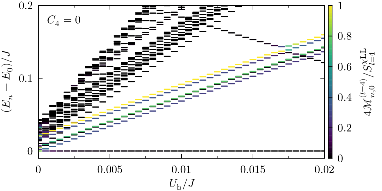
Figure 14: Same as Fig. 13(b), but for an $11\times 11$ lattice.

VII Dipolar excitation

VII.1 Perturbation theory

In this section we explicitly derive the system’s dipole response to a dipolar pulsed excitation

$$\hat{V}(t)=\lambda(t)\sum_{i}x_{i}\hat{n}_{i};$$ (28)

we consider the pulse to have a Gaussian temporal profile $\lambda(t)=\lambda_{d}\exp(-t^{2}/\tau^{2})$. We monitor the time evolution of the system’s dipole moment

$$\hat{O}=\sum_{i}x_{i}\hat{n}_{i}.$$ (29)

We consider our system to start in the ground state $\ket{0}$.

To first order in perturbation theory we get

$$\braket{\hat{O}}(t)\simeq-\frac{2}{\hbar}\,\sum_{n}\text{Im}\left[\int_{-\infty}^{t}dt^{\prime}\,\lambda(t^{\prime})e^{-i\omega_{n,0}(t^{\prime}-t)}|\braket{n}{\hat{O}}{0}|^{2}\right]$$ (30)

where $\omega_{n,0}=(E_{n}-E_{0})/\hbar$ is the energy of the excited state $\ket{n}$. Here we used the fact that $\bra{0}\hat{O}\ket{0}=0$.

In the Laughlin phase, at low energies a single mode alone contributes to the summation; namely the low-energy “dipole” edge mode (see Fig. 1(a) in the main text). We define $\omega_{d}$ to be the frequency of such a transition. Moreover, $|\braket{n}{\hat{O}}{0}|^{2}=\left|\left<n\left|\sum_{i}\frac{x_{i}+iy_{i}}{2}\,\hat{n}_{i}\right|0\right>\right|^{2}=S_{1}/4$. The first equality is a consequence of the lattice fourfold rotational symmetry; the second one comes from the fact that the only contribution to the dipolar static structure factor is exhausted by this single matrix element (see Fig. 1(b,c) in the main text).

If $t\gg\tau$ we can replace the upper integration limit in Eq. (30) with $t\rightarrow\infty$, obtaining

$$\braket{\hat{O}}(t)\simeq-\frac{S_{1}}{2\hbar}\,\text{Im}\left[\widetilde{\lambda}(\omega_{d})e^{i\omega_{d}t}\right]$$ (31)

where we defined the Fourier transform $\widetilde{\lambda}(\omega_{d})=\int_{-\infty}^{\infty}dt^{\prime}\,\lambda(t^{\prime})e^{-i\omega_{d}t^{\prime}}=\lambda_{d}\tau\sqrt{\pi}\,\exp\left[-\left(\frac{\omega_{d}\tau}{2}\right)^{2}\right]$ of the pulsed excitation $\lambda(t)$. This is the equation we quoted in the main text.

To conclude this section, let us notice that in order to control the strength of the perturbation $\tau$ cannot be chosen to be too large, otherwise the pulse becomes adiabatic with respect to the edge modes, as testified by the Fourier factor $\propto\tau\exp\left[-\left(\frac{\omega_{d}\tau}{2}\right)^{2}\right]$. This problem can be easily circumvented in principle by resonantly shaking the lattice with $\lambda(t)=\lambda_{d}\exp(-t^{2}/\tau^{2})\cos(\Omega t)$, $\Omega\approx\omega_{d}$. Then, by neglecting the off-resonant term $\widetilde{\lambda}(\omega_{d}+\Omega)$, one obtains

$$\braket{\hat{O}}(t)\simeq-\frac{S_{1}}{4\hbar}\,\text{Im}\left[\widetilde{\lambda}(\omega_{d}-\Omega)e^{i\omega_{d}t}\right].$$ (32)

Notice that all these results are valid only within the scope of linear perturbation theory. Non-linear effects are discussed in the next section in a two-level approximation.

VII.2 Rabi oscillations

Thanks to the strong non-linearity imposed by the hard-wall condition, contrary to standard chiral Luttinger liquid (or in the presence of weak non-linearities) - the spectrum of the edge modes is not linearly dispersing with the excitation momentum. Highly non-linear behaviour can be seen in Fig. 1 in the main text. The idea is to exploit this non-linearity in order for the system to perform Rabi oscillations between the ground state and the dipole mode as if these two levels constituted an isolated two-level system. In this section we give some mathematical details on the performed calculations.

In Heisenberg’s representation $\ket{\widetilde{\psi}}=e^{i\hat{H}t/\hbar}\ket{\psi}$, Schrödinger equation reads

$$i\hbar\frac{\partial\ket{\widetilde{\psi}}}{\partial t}=\widetilde{V}\ket{\widetilde{\psi}},$$ (33)

where $\widetilde{V}=e^{i\hat{H}t/\hbar}\hat{V}e^{-i\hat{H}t/\hbar}$ is the excitation operator, $\hat{V}=\lambda(t)\hat{O}$. The observable we excite is again dipolar, $\hat{O}=\sum_{i}x_{i}\hat{n}_{i}$. As we briefly commented at the end of the previous section, we resonantly shake the lattice

$$\lambda(t)=\lambda_{d}e^{-t^{2}/\tau^{2}}\,\cos(\Omega t).$$ (34)

If the spectrum of edge modes is linearly dispersing with the momentum, as one would expect for smooth edges in the thermodynamic limit where the chiral Luttinger liquid description is expected to be valid, long excitations of this kind will not only drive a transition from the Laughlin ground state to its dipole moment, but also higher order excitations which on the long run drive the system out of these two levels. However, as we already anticipated, strong non-linearities imposed by the hard-wall confinement together with the small lattices analysed here make these higher-order transitions off-resonant. We can therefore effectively describe the dynamics as being restricted to two levels, and we can expand $\ket{\widetilde{\psi}}=\widetilde{c}_{0}\ket{0}+\widetilde{c}_{1}\ket{1}$: the two states represent the ground state and the lowest-lying dipole state respectively, see Fig. 1 in the main text. Taking the scalar products of Eq. (33) with $\ket{0}$ and $\ket{1}$ we get

$$\begin{cases}i\hbar\frac{\partial\widetilde{c}_{0}}{\partial t}=\widetilde{c}_{1}\bra{0}\widetilde{V}\ket{1}\\ i\hbar\frac{\partial\widetilde{c}_{1}}{\partial t}=\widetilde{c}_{0}\bra{1}\widetilde{V}\ket{0}.\end{cases}$$ (35)

Here, we used the fact that $\bra{0}\hat{O}\ket{0}=\bra{1}\hat{O}\ket{1}=0$ by symmetry. On the other hand, $\bra{1}\hat{O}\ket{0}\equiv d_{x}=|d_{x}|e^{i\alpha}$ is non-zero. The phase can be absorbed into the wavefunction amplitudes by defining $b_{0}=\widetilde{c}_{0}e^{i\alpha/2}$, $b_{1}=\widetilde{c}_{1}e^{-i\alpha/2}$.

Since $\Omega\approx\omega_{d}$ we can neglect fast terms, obtaining

$$\begin{cases}i\frac{\partial{b}_{0}}{\partial t}=\Omega_{R}\,{b}_{1}(t)\,e^{i(\Omega-\omega_{d})t}e^{-t^{2}/\tau^{2}}\\ i\frac{\partial{b}_{1}}{\partial t}=\Omega_{R}\,{b}_{0}(t)\,e^{i(\omega_{d}-\Omega)t}e^{-t^{2}/\tau^{2}}.\end{cases}$$ (36)

Here we defined an effective Rabi frequency

$$\Omega_{R}=\frac{\lambda_{d}|d_{x}|}{2\hbar}.$$ (37)

For simplicity we consider the driving to be resonant, namely $\Omega=\omega_{d}$. The solutions with initial conditions $b_{0}(t\ll\tau)=1$ and $b_{1}(t\ll\tau)=0$ read

$$\begin{cases}{b}_{0}(t)=\cos\left(\Lambda(t)\right)\\ {b}_{1}(t)=-i\sin\left(\Lambda(t)\right)\end{cases} \qquad\Lambda(t)=\frac{1}{2}\sqrt{\pi}\tau\,\Omega_{R}\left(1+\text{erf}\left(\frac{t}{\tau}\right)\right).$$ (38)

We can finally write down the time evolution of the dipole moment

$$\braket{\hat{O}}(t) =2\text{Re}\bigl{(}b_{0}(t)b_{1}^{*}(t)e^{i\omega_{d}t}|d_{x}|\bigr{)}=-|d_{x}|\sin(2\Lambda(t))\,\sin(\omega_{d}t).$$ (39)

As we explained in the previous section, $|d_{x}|=\sqrt{S_{1}}/2=|d|/2$. Therefore, at large times $t\gg\tau$ (since $\text{erf}(t/\tau)\rightarrow 1$) we can write

$$\braket{\hat{O}}(t\gg\tau)=-\frac{|d|}{2}\sin\left(\sqrt{\pi}\tau\,\frac{\lambda_{d}|d|}{2\hbar}\right)\,\sin(\omega_{d}t)$$ (40)

which is the result we quoted in the main text. Notice that the dipole oscillates as a pure sine-wave with an amplitude $\frac{|d|}{2}\sin\left(\sqrt{\pi}\tau\,\frac{\lambda_{d}|d|}{2\hbar}\right)$: this can be interpreted as the system performing Rabi oscillations with frequency $\Omega_{R}=\frac{\lambda_{d}|d|}{\hbar}$, driven over an effective time-window $T=\sqrt{\pi}\tau$.

Notice finally that when $\lambda_{d}|d|\tau/\hbar\ll 1$ it correctly recovers the perturbative result obtained in the previous section, Eq. (32). On the other hand, the strong anharmonicity due to the confinement allows one to dynamically get larger dipole response

$$|\braket{\hat{O}}|\approx\frac{|d|}{2}$$ (41)

provided one can perform a $\pi/2$ pulse which drives the system from its many-body ground state $\ket{0}$ to the coherent and equal superposition $(\ket{0}+\ket{1})/\sqrt{2}$; this in practice is limited by the pulse duration $\sqrt{\pi}\tau$, which is limited by the coherence time of the experiment.

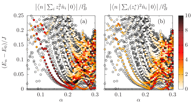
Figure 15: Energies (with respect to the ground state one) for a system of $N=3$ bosons on a $9\times 9$ lattice, as a function of the magnetic field per plaquette $\alpha$. The points have been coloured according to the value of (a) $\mathcal{M}_{n,0}^{(2)}=\left|\braket{n\left missing}{\sum_{i}z_{i}^{2}\hat{n}_{i}}{0}\right|^{2}$ and (b) $\left|\braket{n\left missing}{\sum_{i}(z_{i}^{*})^{2}\hat{n}_{i}}{0}\right|^{2}$.

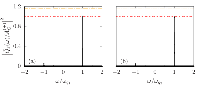
Figure 16: Square modulus of the Fourier transform $\tilde{Q}_{z}(\omega)$ of the quadrupole response $Q_{z}(t)$ at long times (after the pulsed excitation has been turned off), as a function of the frequency $\omega$ (normalized to the relevant quadrupolar frequencies (a) $\omega_{q_{1}}$ and (b) $\omega_{q_{2}}$. In both cases, two narrow peaks at $\pm 1$ can be seen: Wen’s sum rule Eq. (9) can be studied by analysing the positive frequency peaks in the two cases. The yellow horizontal line is the linear perturbation theory prediction (see Eq. (48)); the red one instead is the non-linear two-level system prediction (see Eq. (49)).

VIII Quadrupolar excitation

VIII.1 Perturbation theory

Since the non-linearities introduced by the hard-wall confinement strongly split the two quadrupolar edge-modes (see Fig. 1(c) in the main text), the quadrupolar static structure factor is most easily measured by separately addressing the two transitions so as to measure the two transition matrix elements. In this section, we label these two states as $\ket{q_{1}}$ and $\ket{q_{2}}$.

We consider the ground state to be excited by a rotating saddle potential

$$\hat{V}=\lambda_{Q}\left(\hat{O}_{x^{2}-y^{2}}\cos(\Omega t)+\hat{O}_{xy}\sin(\Omega t)\right)e^{-t^{2}/\tau^{2}},$$ (42)

where

$$\hat{O}_{x^{2}-y^{2}} =\sum_{i}(x_{i}^{2}-y_{i}^{2})\,\hat{n}_{i}$$ (43)

$$\hat{O}_{xy} =\sum_{i}2x_{i}y_{i}\,\hat{n}_{i}.$$ (44)

The perturbation can be rewritten in terms of the complex combination $z_{i}=x_{i}+iy_{i}$ as

$$\hat{V}=\frac{1}{2}\lambda_{Q}\left(\hat{O}_{z^{2}}^{\vphantom{\dagger}}e^{-i\Omega t}+\hat{O}_{z^{2}}^{\dagger}e^{+i\Omega t}\right)e^{-t^{2}/\tau^{2}}$$ (45)

with $\hat{O}_{z^{2}}=\sum_{i}z_{i}^{2}\,\hat{n}_{i}=\hat{O}_{x^{2}-y^{2}}+i\hat{O}_{xy}$.

If the system was fully rotationally symmetric, due to angular momentum conservation we would have $\braket{q_{1}}{\hat{O}_{z^{2}}^{\dagger}}{0}=\braket{q_{2}}{\hat{O}_{z^{2}}^{\dagger}}{0}=0$. However, our system has only fourfold rotational symmetry. As a consequence, these matrix elements do not vanish, even though we find them to be significantly smaller (by a factor $\sim 10$). We show a comparison in Fig. 15. The purpose of the modulation at frequency $\Omega$ is to make transitions driven by $\hat{O}_{z^{2}}^{\dagger}$ from $\ket{0}$ to the quadrupole modes $\{\ket{q_{1}},\ket{q_{2}}\}$ small; this allows one to focus instead on the transitions driven by $\hat{O}_{z^{2}}^{\vphantom{\dagger}}$, of which we want to reconstruct the static structure factor.

Using linear-order perturbation theory we write

$$Q_{z}(t)\simeq\frac{i}{\hbar}\int_{-\infty}^{t}\braket{\widetilde{V}(t^{\prime})\widetilde{O}_{z^{2}}(t)-\widetilde{O}_{z^{2}}(t)\widetilde{V}(t^{\prime})}\,dt^{\prime}$$ (46)

where the tilde denotes Heisenberg representation with respect to $\hat{H}$ and we defined $Q_{z}(t)=\braket{\hat{O}_{z^{2}}}(t)$. Notice that $\hat{O}_{z^{2}}(t)=\hat{O}_{x^{2}-y^{2}}+i\hat{O}_{xy}$ is a complex linear combination of two physical observables.

Neglecting off-resonant terms in Eq. (46) we obtain

$$Q_{z}(t)=\frac{i}{2\hbar}\int_{-\infty}^{t}dt^{\prime}\lambda(t^{\prime})\sum_{n}\left(e^{i\omega_{n,0}t}e^{i(\Omega-\omega_{n,0})t^{\prime}}|\braket{n}{\hat{O}_{z^{2}}^{\vphantom{\dagger}}}{0}|^{2}-e^{-i\omega_{n,0}t}e^{-i(\Omega-\omega_{n,0})t^{\prime}}\braket{0}{\hat{O}_{z^{2}}^{\vphantom{\dagger}}}{n}\braket{n}{\hat{O}_{z^{2}}^{\vphantom{\dagger}}}{0}\right).$$ (47)

For large enough $\tau$ and $\Omega\simeq\omega_{q}$ only one of the quadrupole modes $\ket{q}$ will be excited. For $t\gg\tau$ we write

$$Q_{z}(t\gg\tau)=\frac{i}{2\hbar}\left(e^{i\omega_{q}t}\widetilde{\lambda}(\omega_{q}-\Omega)|\braket{q}{\hat{O}_{z^{2}}^{\vphantom{\dagger}}}{0}|^{2}-e^{-i\omega_{q}t}\widetilde{\lambda}^{*}(\omega_{q}-\Omega)\braket{0}{\hat{O}_{z^{2}}^{\vphantom{\dagger}}}{q}\braket{q}{\hat{O}_{z^{2}}^{\vphantom{\dagger}}}{0}\right).$$ (48)

By resolving the two frequencies, for example through Fourier analysis, the relevant amplitude $|\braket{q}{\hat{O}_{z^{2}}^{\vphantom{\dagger}}}{0}|^{2}$ can be extracted; once this is done for the first quadrupole mode $\ket{q_{1}}$, the same can be done for the second one, $\ket{q_{2}}$ and one can reconstruct the static structure factor and match it with Wen’s prediction.

We show the discrete Fourier transforms (taken only for $t\gtrsim\tau$) of $Q_{z}(t)$ for the two quadrupolar transitions in Fig. 16. Frequencies are measured in units of the relevant transition frequency $\omega_{q}$. Peaks at $\omega/\omega_{q}=\pm 1$ can be seen; as expected, the one at negative frequency, which emerges because of the reduced rotational symmetry of the lattice, can be seen to be smaller than the relevant one at positive frequency. The peak-amplitude of the latter is compared with the amplitude that we obtain from the perturbation theory result (yellow-dashed line) and with the non-linear two-level system result Eq. (49). It can be seen that the latter compares successfully with the numerical results and can be used to estimate the relevant matrix element $|\braket{q}{\hat{O}_{z^{2}}}{0}|^{2}$.

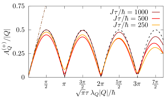
Figure 17: Positive frequency amplitude of $Q_{z}(t\gg\tau)$ as a function of the pulse angle $\Omega_{R}T$ ($T=\sqrt{\pi}\tau$), for different values of the pulse duration $\tau$. The resonant two-level Rabi oscillation prediction (see Eq. (49)) is shown as a black-dashed line, and the linear approximation (see Eq. (48)) is shown as a dash-dotted brown line.

VIII.2 Rabi oscillations

Analogously to the dipolar-excitation case, due to the strong non-linearities imposed by the lattice the ground-state to quadrupole transition can form an isolated two-level manifold within the exponentially large set of many-body states. The quantitative analysis is the same as in the case of the dipolar excitation, with the additional complication of the reduced rotational symmetry of the lattice. We find, for a resonant excitation ($\Omega=\omega_{q}$)

$$Q_{z}(t\gg\tau)=i\,\underbrace{\frac{\left|Q\right|}{2}\sin\left(\sqrt{\pi}\tau\,\frac{\lambda_{Q}\left|Q\right|}{\hbar}\right)}_{A_{Q}^{(+)}}\,e^{i\omega_{q}t}-i\underbrace{\frac{Q^{\prime}e^{i\alpha}}{2}\sin\left(\sqrt{\pi}\tau\,\frac{\lambda_{Q}\left|Q\right|}{\hbar}\right)}_{A_{Q}^{(-)}}\,e^{-i\omega_{q}t}$$ (49)

where $Q=\braket{q}{\hat{O}_{z^{2}}^{\vphantom{\dagger}}}{0}$, $Q^{\prime}=\braket{0}{\hat{O}_{z^{2}}^{\vphantom{\dagger}}}{q}$ and $\alpha=\arg\left(Q\right)$. To linear order in perturbation theory, this result reduces to the perturbative one given in Eq. (48).

We compare the numerical amplitude of the peak at positive frequency, $A_{Q}^{(+)}$, with the above result Eq. (49) in Fig. 17, for the case of the lower quadrupolar transition. It can be seen that for long-enough pulses the predictions nicely match the analytical result.

References

- Tsui et al. [1982] D. C. Tsui, H. L. Stormer, and A. C. Gossard, Two-Dimensional Magnetotransport in the Extreme Quantum Limit, Phys. Rev. Lett. 48, 1559 (1982) .
- von Klitzing et al. [2020] K. von Klitzing, T. Chakraborty, P. Kim, V. Madhavan, X. Dai, J. McIver, Y. Tokura, L. Savary, D. Smirnova, A. M. Rey, C. Felser, J. Gooth, and X. Qi, 40 years of the quantum Hall effect, Nature Reviews Physics 2, 397 (2020) .
- Laughlin [1983] R. B. Laughlin, Anomalous Quantum Hall Effect: An Incompressible Quantum Fluid with Fractionally Charged Excitations, Phys. Rev. Lett. 50, 1395 (1983) .
- Arovas et al. [1984] D. Arovas, J. R. Schrieffer, and F. Wilczek, Fractional Statistics and the Quantum Hall Effect, Phys. Rev. Lett. 53, 722 (1984) .
- Nayak et al. [2008] C. Nayak, S. H. Simon, A. Stern, M. Freedman, and S. D. Sarma, Non-Abelian anyons and topological quantum computation, Reviews of Modern Physics 80, 1083 (2008) .
- Wen [1990a] X. G. Wen, Electrodynamical properties of gapless edge excitations in the fractional quantum Hall states, Phys. Rev. Lett. 64, 2206 (1990a) .
- Wen [1990b] X. G. Wen, Chiral Luttinger liquid and the edge excitations in the fractional quantum Hall states, Phys. Rev. B 41, 12838 (1990b) .
- Wen [1991a] X. G. Wen, Gapless boundary excitations in the quantum Hall states and in the chiral spin states, Phys. Rev. B 43, 11025 (1991a) .
- Wen [1991b] X.-G. Wen, Edge transport properties of the fractional quantum Hall states and weak-impurity scattering of a one-dimensional charge-density wave, Phys. Rev. B 44, 5708 (1991b) .
- Wen [1995] X.-G. Wen, Topological orders and edge excitations in fractional quantum Hall states, Adv. Phys. 44, 405 (1995) .
- Wen [1992] X.-G. Wen, Theory of the Edge States in Fractional Quantum Hall Effects, International Journal of Modern Physics B 06, 1711 (1992) .
- Chang [2003] A. M. Chang, Chiral Luttinger liquids at the fractional quantum Hall edge, Rev. Mod. Phys. 75, 1449 (2003) .
- Wen [2019] X.-G. Wen, Choreographed entanglement dances: Topological states of quantum matter, Science 363, eaal3099 (2019) .
- de-Picciotto et al. [1997] R. de-Picciotto, M. Reznikov, M. Heiblum, V. Umansky, G. Bunin, and D. Mahalu, Direct observation of a fractional charge, Nature (London) 389, 162 (1997) .
- Chang et al. [1996] A. M. Chang, L. N. Pfeiffer, and K. W. West, Observation of Chiral Luttinger Behavior in Electron Tunneling into Fractional Quantum Hall Edges, Phys. Rev. Lett. 77, 2538 (1996) .
- Banerjee et al. [2018] M. Banerjee, M. Heiblum, V. Umansky, D. E. Feldman, Y. Oreg, and A. Stern, Observation of half-integer thermal Hall conductance, Nature (London) 559, 205 (2018) .
- Aharon Melcer et al. [2023] R. Aharon Melcer, S. Konyzheva, M. Heiblum, and V. Umansky, Direct Determination of the Topological Thermal Conductance via Local Power Measurement, Nature Physics (2023), https://doi.org/10.1038/s41567-022-01885-5 .
- Nakamura et al. [2020] J. Nakamura, S. Liang, G. C. Gardner, and M. J. Manfra, Direct observation of anyonic braiding statistics, Nature Physics 16, 931 (2020) .
- Bartolomei et al. [2020] H. Bartolomei, M. Kumar, R. Bisognin, A. Marguerite, J. M. Berroir, E. Bocquillon, B. Plaçais, A. Cavanna, Q. Dong, U. Gennser, Y. Jin, and G. Fève, Fractional statistics in anyon collisions, Science 368, 173 (2020) .
- Nakamura et al. [2023] J. Nakamura, S. Liang, G. C. Gardner, and M. J. Manfra, Fabry-Pérot Interferometry at the Fractional Quantum Hall State, Phys. Rev. X 13, 041012 (2023) .
- Cooper [2008] N. Cooper, Rapidly rotating atomic gases, Advances in Physics 57, 539 (2008) .
- Bloch et al. [2008] I. Bloch, J. Dalibard, and W. Zwerger, Many-body physics with ultracold gases, Rev. Mod. Phys. 80, 885 (2008) .
- Cooper et al. [2019] N. R. Cooper, J. Dalibard, and I. B. Spielman, Topological bands for ultracold atoms, Rev. Mod. Phys. 91, 015005 (2019) .
- Goldman et al. [2014] N. Goldman, G. Juzeliū nas, P. Öhberg, and I. B. Spielman, Light-induced gauge fields for ultracold atoms, Reports on Progress in Physics 77, 126401 (2014) .
- Carusotto et al. [2020] I. Carusotto, A. Houck, A. Kollár, P. Roushan, D. Schuster, and J. Simon, Photonic materials in circuit quantum electrodynamics, Nature Physics 16, 268 (2020) .
- Carusotto and Ciuti [2013] I. Carusotto and C. Ciuti, Quantum fluids of light, Rev. Mod. Phys. 85, 299 (2013) .
- Ozawa et al. [2019] T. Ozawa, H. M. Price, A. Amo, N. Goldman, M. Hafezi, L. Lu, M. C. Rechtsman, D. Schuster, J. Simon, O. Zilberberg, and I. Carusotto, Topological photonics, Rev. Mod. Phys. 91, 015006 (2019) .
- Gemelke et al. [2010] N. Gemelke, E. Sarajlic, and S. Chu, Rotating Few-body Atomic Systems in the Fractional Quantum Hall Regime, (2010).
- Léonard et al. [2023] J. Léonard, S. Kim, J. Kwan, P. Segura, F. Grusdt, C. Repellin, N. Goldman, and M. Greiner, Realization of a fractional quantum Hall state with ultracold atoms, Nature 619, 495–499 (2023) .
- Lunt et al. [2024] P. Lunt, P. Hill, J. Reiter, P. M. Preiss, M. Gałka, and S. Jochim, Realization of a Laughlin state of two rapidly rotating fermions, arXiv:2402.14814 [cond-mat.quant-gas] (2024).
- Clark et al. [2020] L. W. Clark, N. Schine, C. Baum, N. Jia, and J. Simon, Observation of Laughlin states made of light, Nature (London) 582, 41 (2020) .
- Wang et al. [2024] C. Wang, F.-M. Liu, M.-C. Chen, H. Chen, X.-H. Zhao, C. Ying, Z.-X. Shang, J.-W. Wang, Y.-H. Huo, C.-Z. Peng, X. Zhu, C.-Y. Lu, and J.-W. Pan, Realization of fractional quantum Hall state with interacting photons, arXiv:2401.17022 [quant-ph] (2024).
- Tran et al. [2017] D. T. Tran, A. Dauphin, A. G. Grushin, P. Zoller, and N. Goldman, Probing topology by “heating”: Quantized circular dichroism in ultracold atoms, Science Advances 3 (2017), 10.1126/sciadv.1701207 .
- Račiūnas et al. [2018] M. Račiūnas, F. N. Ünal, E. Anisimovas, and A. Eckardt, Creating, probing, and manipulating fractionally charged excitations of fractional Chern insulators in optical lattices, Phys. Rev. A 98, 063621 (2018) .
- Repellin and Goldman [2019] C. Repellin and N. Goldman, Detecting Fractional Chern Insulators through Circular Dichroism, Phys. Rev. Lett. 122, 166801 (2019) .
- Macaluso et al. [2020] E. Macaluso, T. Comparin, R. O. Umucal ılar, M. Gerster, S. Montangero, M. Rizzi, and I. Carusotto, Charge and statistics of lattice quasiholes from density measurements: A tree tensor network study, Phys. Rev. Res. 2, 013145 (2020) .
- Umucalılar [2023] R. O. Umucalılar, Bulk density signatures of a lattice quasihole with very few particles, Phys. Rev. A 108, L061302 (2023) .
- Kjäll and Moore [2012] J. A. Kjäll and J. E. Moore, Edge excitations of bosonic fractional quantum Hall phases in optical lattices, Phys. Rev. B 85, 235137 (2012) .
- Luo et al. [2013] W.-W. Luo, W.-C. Chen, Y.-F. Wang, and C.-D. Gong, Edge excitations in fractional Chern insulators, Phys. Rev. B 88, 161109 (2013) .
- Binanti et al. [2023] F. Binanti, N. Goldman, and C. Repellin, Edge mode spectroscopy of fractional Chern insulators, arXiv:2306.01624 [cond-mat.quant-gas] (2023).
- Fern and Simon [2017] R. Fern and S. H. Simon, Quantum Hall edges with hard confinement: Exact solution beyond Luttinger liquid, Phys. Rev. B 95, 201108 (2017) .
- Macaluso and Carusotto [2017] E. Macaluso and I. Carusotto, Hard-wall confinement of a fractional quantum Hall liquid, Phys. Rev. A 96, 043607 (2017) .
- Macaluso and Carusotto [2018] E. Macaluso and I. Carusotto, Ring-shaped fractional quantum Hall liquids with hard-wall potentials, Phys. Rev. A 98, 013605 (2018) .
- Nardin and Carusotto [2023a] A. Nardin and I. Carusotto, Linear and nonlinear edge dynamics of trapped fractional quantum Hall droplets, Phys. Rev. A 107, 033320 (2023a) .
- Nardin and Carusotto [2023b] A. Nardin and I. Carusotto, Refermionized theory of the edge modes of a fractional quantum Hall cloud, arXiv:2305.00291 [cond-mat.str-el] (2023b).
- Kastner [1992] M. A. Kastner, The single-electron transistor, Rev. Mod. Phys. 64, 849 (1992) .
- Imamoḡlu et al. [1997] A. Imamoḡlu, H. Schmidt, G. Woods, and M. Deutsch, Strongly Interacting Photons in a Nonlinear Cavity, Phys. Rev. Lett. 79, 1467 (1997) .
- Verger et al. [2006] A. Verger, C. Ciuti, and I. Carusotto, Polariton quantum blockade in a photonic dot, Phys. Rev. B 73, 193306 (2006) .
- Birnbaum et al. [2005] K. M. Birnbaum, A. Boca, R. Miller, A. D. Boozer, T. E. Northup, and H. J. Kimble, Photon blockade in an optical cavity with one trapped atom, Nature 436, 87 (2005) .
- Lang et al. [2011] C. Lang, D. Bozyigit, C. Eichler, L. Steffen, J. M. Fink, A. A. Abdumalikov, M. Baur, S. Filipp, M. P. da Silva, A. Blais, and A. Wallraff, Observation of Resonant Photon Blockade at Microwave Frequencies Using Correlation Function Measurements, Phys. Rev. Lett. 106, 243601 (2011) .
- Rabl [2011] P. Rabl, Photon Blockade Effect in Optomechanical Systems, Phys. Rev. Lett. 107, 063601 (2011) .
- Nunnenkamp et al. [2011] A. Nunnenkamp, K. Børkje, and S. M. Girvin, Single-Photon Optomechanics, Phys. Rev. Lett. 107, 063602 (2011) .
- Sørensen et al. [2005a] A. S. Sørensen, E. Demler, and M. D. Lukin, Fractional Quantum Hall States of Atoms in Optical Lattices, Phys. Rev. Lett. 94, 086803 (2005a) .
- Sørensen et al. [2005b] A. S. Sørensen, E. Demler, and M. D. Lukin, Fractional Quantum Hall States of Atoms in Optical Lattices, Phys. Rev. Lett. 94, 086803 (2005b) .
- Hafezi et al. [2007] M. Hafezi, A. S. Sørensen, E. Demler, and M. D. Lukin, Fractional quantum Hall effect in optical lattices, Phys. Rev. A 76, 023613 (2007) .
- Gerster et al. [2017] M. Gerster, M. Rizzi, P. Silvi, M. Dalmonte, and S. Montangero, Fractional quantum Hall effect in the interacting Hofstadter model via tensor networks, Phys. Rev. B 96, 195123 (2017) .
- Hofstadter [1976] D. R. Hofstadter, Energy levels and wave functions of Bloch electrons in rational and irrational magnetic fields, Phys. Rev. B 14, 2239 (1976) .
- Palm et al. [2021] F. A. Palm, M. Buser, J. Léonard, M. Aidelsburger, U. Schollwöck, and F. Grusdt, Bosonic Pfaffian state in the Hofstadter-Bose-Hubbard model, Phys. Rev. B 103, L161101 (2021) .
- Möller and Cooper [2009] G. Möller and N. R. Cooper, Composite Fermion Theory for Bosonic Quantum Hall States on Lattices, Phys. Rev. Lett. 103, 105303 (2009) .
- Möller and Cooper [2015] G. Möller and N. R. Cooper, Fractional Chern Insulators in Harper-Hofstadter Bands with Higher Chern Number, Phys. Rev. Lett. 115, 126401 (2015) .
- Boesl et al. [2022] J. Boesl, R. Dilip, F. Pollmann, and M. Knap, Characterizing fractional topological phases of lattice bosons near the first Mott lobe, Physical Review B 105 (2022), 10.1103/physrevb.105.075135 .
- Note [1] See Supplemental Material for a derivation of the structure factor value in the thermodynamic limit, a brief derivation of Kohn’s theorem, the link between the structure factor and the transverse conductivity in the bulk, additional numerical results (different lattice sizes and particle numbers, as well as the overlaps with discretized model wavefunctions and an analysis of the energy levels and relevant matrix elements as a function of an additional harmonic confinement) and for the explicit calculations for the relevant observables time-evolution, both for the dipolar and quadrupolar excitations and in the perturbative/non-linear regimes.
- Repellin et al. [2020] C. Repellin, J. Léonard, and N. Goldman, Fractional Chern insulators of few bosons in a box: Hall plateaus from center-of-mass drifts and density profiles, Phys. Rev. A 102, 063316 (2020) .
- Imambekov et al. [2012] A. Imambekov, T. L. Schmidt, and L. I. Glazman, One-dimensional quantum liquids: Beyond the Luttinger liquid paradigm, Rev. Mod. Phys. 84, 1253 (2012) .
- Fern et al. [2018] R. Fern, R. Bondesan, and S. H. Simon, Effective edge state dynamics in the fractional quantum Hall effect, Phys. Rev. B 98, 155321 (2018) .
- Cazalilla [2003] M. A. Cazalilla, Surface modes of ultracold atomic clouds with a very large number of vortices, Phys. Rev. A 67, 063613 (2003) .
- Carusotto et al. [2010] I. Carusotto, T. Volz, and A. Imamoğlu, Feshbach blockade: Single-photon nonlinear optics using resonantly enhanced cavity polariton scattering from biexciton states, Europhysics Letters 90, 37001 (2010) .
- Goldman et al. [2012] N. Goldman, J. Beugnon, and F. Gerbier, Detecting Chiral Edge States in the Hofstadter Optical Lattice, Phys. Rev. Lett. 108, 255303 (2012) .
- Kamiyama et al. [2022] A. Kamiyama, M. Matsuura, J. N. Moore, T. Mano, N. Shibata, and G. Yusa, Real-time and space visualization of excitations of the =1 /3 fractional quantum Hall edge, Physical Review Research 4, L012040 (2022) .
- Cohen-Tannoudji et al. [1998] C. Cohen-Tannoudji, J. Dupont-Roc, and G. Grynberg, Atom-Photon Interactions: Basic Processes and Applications (Wiley, 1998).
- Haroche and Raimond [2013] S. Haroche and J.-M. Raimond, Exploring the quantum: atoms, cavities, and photons, first published in paperback ed., Oxford graduate texts (Oxford University Press, Oxford, 2013).
- Anwar et al. [2021] A. Anwar, C. Perumangatt, F. Steinlechner, T. Jennewein, and A. Ling, Entangled photon-pair sources based on three-wave mixing in bulk crystals, Review of Scientific Instruments 92, 041101 (2021) .
- Bettelheim et al. [2006] E. Bettelheim, A. G. Abanov, and P. Wiegmann, Nonlinear Quantum Shock Waves in Fractional Quantum Hall Edge States, Phys. Rev. Lett. 97, 246401 (2006) .
- Wiegmann [2012] P. Wiegmann, Nonlinear Hydrodynamics and Fractionally Quantized Solitons at the Fractional Quantum Hall Edge, Phys. Rev. Lett. 108, 206810 (2012) .
- Mahmoodian et al. [2020] S. Mahmoodian, G. Calajó, D. E. Chang, K. Hammerer, and A. S. Sørensen, Dynamics of Many-Body Photon Bound States in Chiral Waveguide QED, Phys. Rev. X 10, 031011 (2020) .
- Wagner et al. [2019] G. Wagner, D. X. Nguyen, D. L. Kovrizhin, and S. H. Simon, Interaction Effects and Charge Quantization in Single-Particle Quantum Dot Emitters, Phys. Rev. Lett. 122, 127701 (2019) .
- De Bernardis et al. [2023] D. De Bernardis, F. S. Piccioli, P. Rabl, and I. Carusotto, Chiral Quantum Optics in the Bulk of Photonic Quantum Hall Systems, PRX Quantum 4, 030306 (2023) .
- Kohn [1961] W. Kohn, Cyclotron Resonance and de Haas-van Alphen Oscillations of an Interacting Electron Gas, Phys. Rev. 123, 1242 (1961) .
- Note [2] Namely, it does not rely on the assumption of dealing with a Laughlin wavefunction, but rather on having a single chiral edge-mode satisfying Eq. (21\@@italiccorr).
- Halperin and Jain [2020] B. I. Halperin and J. K. Jain, Fractional Quantum Hall Effects (WORLD SCIENTIFIC, 2020).