Bondi-Hoyle-Lyttleton accretion onto a rotating black hole with ultralight scalar hair

Abstract

We present a numerical study of relativistic Bondi-Hoyle-Lyttleton (BHL) accretion onto an asymptotically flat black hole with synchronized hair. The hair is sourced by an ultralight, complex scalar field, minimally coupled to Einstein’s gravity. Our simulations consider a supersonic flow parametrized by the asymptotic values of the fluid quantities and a sample of hairy black holes with different masses, angular momenta, and amount of scalar hair. For all models, steady-state BHL accretion solutions are attained that are characterized by the presence of a shock-cone and a stagnation point downstream. For the models of the sample with the largest component of scalar field, the shock-cone envelops fully the black hole, transitioning into a bow-shock, and the stagnation points move further away downstream. Analytical expressions for the mass accretion rates are obtained after fitting the numerical results, which can be used to analyze black-hole formation scenarios in the presence of ultralight scalar fields. The formation of a shock-cone leads to regions where sound waves can be trapped and resonant oscillations excited. We measure the frequencies of such quasi-periodic oscillations and point out a possible association with quasi-periodic oscillations in the X-ray light curve of Sgr A* and microquasars.

1 Introduction

Active galactic nuclei (AGNs) are powered by the accretion of gas onto their central supermassive black holes (SMBHs) and emit intense electromagnetic radiation in a broad range of frequencies. Observations of the plasma moving around regions close to the horizon of SMBHs are now possible thanks to the Event Horizon Telescope (EHT), which recently imaged the black hole at the center of the galaxy M87 [1] and of the Milky Way [2]. Black holes are one of the most exciting outcomes of relativistic astrophysics and general relativity. From a mathematical point of view, there are no restrictions on the black hole’s mass. On the other hand, astronomical observations clearly indicate the evidence for astrophysical black holes in two mass windows only: the stellar-mass range ($4\,M_{\odot}\lesssim M_{\rm BH}\lesssim 80\,M_{\odot}$) [3, 4] and the supermassive range ($10^{6}\,M_{\odot}\lesssim M_{\rm BH}\lesssim 10^{9}\,M_{\odot}$) [5, 6, 1]. However, the LIGO-Virgo-KAGRA scientific collaboration (LVK) has reported the detection of gravitational-wave transient GW190521[7], an intermediate-mass black hole of $150\,M_{\odot}$ resulting from the merger of two black holes of masses $85\,M_{\odot}$ and $66\,M_{\odot}$. The nature of this source remains somewhat uncertain (see e.g., [8, 9, 10, 11, 12] for alternative interpretations). In addition, explaining the masses of SMBHs is still an important open problem in astrophysics. One approach to this problem assumes that the large masses of SMBHs are the result of matter accretion onto black hole seeds [13, 14, 15]. Therefore, understanding the details of matter accretion onto black holes is of great relevance on a series of timely problem in gravitational-wave astronomy.

When considering the dynamics of gas around a point mass, one of the most used models was developed by Bondi, Hoyle and Lyttleton (BHL) [16, 17, 18]. The BHL model assumes accretion onto a central compact object moving in a homogeneous distribution of gas and has been widely employed in different astrophysical scenarios, via numerical studies in the Newtonian regime [19, 20, 21, 22, 23, 24, 25, 26, 27, 28, 29, 30]. A historical overview of the development and numerical modeling of BHL accretion studies can be found in [31, 32]. The validity of a Newtonian approach breaks down when the accreting object is a black hole or a neutron star, as general relativistic effects become important, especially when capturing the flow dynamics close to the black hole horizon (see, e.g., Ref. [33], where a Newtonian and relativistic treatment of mass accretion in a common-envelope scenario are contrasted). This motivated the first numerical works dedicated to studying the morphological patterns in the vicinity of a black hole as well as to compute the associated accretion rates of mass and momentum [34, 35, 36, 37, 38]. Subsequently, many simulations have investigated the BHL mechanism in the context of relativistic astrophysics [39, 40, 41, 42], becoming increasingly realistic (and more complex) by including magnetic fields [43, 44, 45], radiative terms [46], density and velocity gradients [47, 48], and small rigid bodies around the black hole [49]. More recently, the role of BHL accretion in the common envelope phase in the evolution of binary systems has also been investigated by [33].

If SMBHs result from accretion onto black-hole seeds, a key question is to determine the interplay between baryons and dark matter in this scenario [13, 50, 51, 52, 53, 54]. In this respect, scalar fields have been proposed to play the role of dark matter, first at galactic scale [55, 56] and then at cosmic scale [57, 58]. Scalar fields interacting with gravity could therefore play a role in understanding the physics associated with black holes, in particular its potential impact on SMBH formation.

Scalar field accretion onto black holes has been already explored in different works. In the context of the ultra-light scalar fields proposed as constituents of dark matter halos, it has been shown that the accretion rate would be small over the lifetime of a typical halo, and hence the central SMBHs could coexist with scalar-field halos [59]. The study of scalar-field accretion has also been carried out on the spacetime background of boson stars [60] and black holes [61, 62, 63] using “Scri” ($\mathcal{I}$)-fixing conformal compactification, that is, including future null infinity $\mathcal{I}^{+}$ in the numerical simulations. In the former case, the scalar field shows quasi-normal mode oscillations only for boson star configurations that are compact enough, where no signs of tail decay were found. In the latter, an extremely high dispersion rate of the scalar field density was found.

The possible existence of equilibrium configurations between ultralight scalar fields and black holes in general relativity has also been addressed in the literature. In [64, 65] it was shown that a massive scalar field surrounding a Schwarzschild black hole can survive for arbitrarily long times, as quasi-bound states, forming scalar “wigs”. Moreover, in the context of the nonlinear evolution of massless scalar fields (also accounting for the evolution of the spacetime), Ref. [66] showed that scalar fields are allowed to survive outside black holes and may eventually have lifetimes consistent with cosmological timescales. Further studies have confirmed the existence of such long-lived states [67, 68, 69, 70]. In addition to the idea that scalar fields can survive for long timescales around black holes, Ref. [71] showed that the gravitational radiation emitted by a Schwarzschild black hole when a massive scalar field is accreted exhibits a distinctive signature, a wiggly tail, in the late-time behavior of the signal.

Eventually, true equilibrium states between ultralight scalar fields and black holes in general relativity were found [72, 73]. A new family of solutions of the Einstein-Klein-Gordon field equations, where the scalar field is complex, massive, and minimally coupled to general relativity, was derived in Ref. [72], to which we will hereafter refer to as “hairy black holes” (HBHs). These solutions describe asymptotically flat rotating black holes with scalar hair that are regular outside of the event horizon and have the following properties:

• are supported by rotation and have no static limit

• have a conserved continuous Noether charge $q$ measuring the scalar hair

• have a Kerr limit when $q=0$

• have a solitonic limit when $q=1$

For more details on the construction of the solutions and their different properties see [73]. The stability of these hairy Kerr black holes was discussed in [74, 75]. In particular, it was shown through numerical analysis that the superradiant instability appears for those solutions [74], but the corresponding timescale increases with the black-hole mass and can be larger than the age of the Universe for sufficiently (super)massive black holes [75]. Therefore, these HBHs provide an interesting model to study the interplay between the accretion of baryonic matter and dark matter in the context of SMBH-formation modeling.

There exist studies aimed at assessing the astrophysical relevance of the aforementioned HBHs [72, 73]. For instance, Ref. [76] investigated the shadow produced by HBHs using backward ray tracing; see also [77, 78]. The extension to electrically charged black holes (Kerr-Newman solution) with scalar hair can be found in [79]. Properties of geodesic motion and its relation to quasi-periodic oscillations (QPOs) have been considered in [80], while the X-ray spectroscopy has been addressed in [81]. More recently, HBHs have been used to build relativistic stationary models of magnetized tori in the test-fluid limit [82, 83].

In this paper, we initiate a program to numerically model relativistic BHL accretion onto an asymptotically flat rotating HBH [72]. In this first investigation, we assume the test-fluid approximation and neglect the evolution of the gravitational field and of the scalar field, concentrating only on the dynamics of the fluid. The simulations have revealed that the morphology of the flow past HBHs is similar to that found for BHL accretion onto a Kerr black hole and that also in this case an upstream bow-shock and a downstream shock-cone can be produced and whose properties depend on the relative strength of the scalar field over the central black hole. At the same time, the phenomenology of the flow is also richer because of the increased possibility of trapping pressure modes in the cavities that are produced, either by the fluid or by the scalar field, and that can in principle be observed in terms of QPOs.

The organization of the paper is the following: in Sec. 2 we briefly describe the theory associated with our specific family of HBHs as well as the sample of (four) configurations we consider. In Sec. 3 we present the mathematical framework for the general-relativistic hydrodynamics equations and the numerical setup used. Section 4 discusses the accretion dynamics and morphology, along with the mass and angular momentum accretion rates for all HBHs models of our study. Moreover, in Sec. 5 we show an astrophysical application of our model by measuring frequencies of oscillation of resonant cavities of our system and comparing them with the QPO frequencies observed in Sgr A* and several microquasar sources. Finally, Sec. 6 summarizes our conclusions. Throughout the paper, Greek indices run from 0 to 3 while Latin ones run from 1 to 3. Additionally, equations are written in geometrized units where $G=c=1$.

2 Rotating Black Holes with Scalar Hair

Model	$M_{\rm ADM}$	$J_{\rm ADM}$	$a_{\rm ADM}$	$a_{\rm BH}$	$p_{\rm EH}$	$q_{\rm EH}$	$p$	$q$	$\Omega_{\rm EH}$	$r_{\rm EH}$	$M_{\phi}/M_{\rm BH}$
HBH-a	$0.415$	$0.172$	$0.999$	$0.971$	$0.947$	$0.872$	$0.053$	$0.128$	$0.975$	$0.200$	$0.06$
HBH-b	$0.933$	$0.739$	$0.849$	$2.075$	$0.251$	$0.154$	$0.749$	$0.846$	$0.820$	$0.100$	$2.98$
HBH-c	$0.539$	$0.495$	$1.704$	$0.617$	$0.091$	$0.003$	$0.909$	$0.997$	$0.980$	$0.101$	$9.99$
HBH-d	$0.975$	$0.850$	$0.894$	$5.519$	$0.018$	$0.002$	$0.982$	$0.998$	$0.680$	$0.040$	$54.56$

Table 1: Spacetime properties corresponding to our HBH solutions: reported are the ADM mass $M_{\rm ADM}$ and total angular momentum and $J_{\rm ADM}$, together with the fractions of energy $(p$) and angular momentum ($q$) measured at the event horizon (subscript ${\rm EH}$) and in the exterior scalar field. Thus $p_{\rm EH}:=M_{\rm BH}/M_{\rm ADM}$, $q_{\rm EH}:=J_{\rm BH}/J$, $p:=M_{\phi}/M_{\rm ADM}=1-p_{\rm EH}$, and $q:=J_{\phi}/J_{\rm ADM}=1-q_{\rm EH}$. For convenience we redefine the dimensionless spin parameters as $a_{\rm ADM}:=J_{\rm ADM}/M_{\rm ADM}^{2}$ and $a_{\rm BH}:=J_{\rm BH}/M_{\rm BH}^{2}$. The black-hole mass and angular momentum, $M_{\rm BH}$ and $J_{\rm BH}$, are computed as Komar surface integrals; the scalar field mass and angular momentum, $M_{\phi}$ and $J_{\phi}$, are computed as volume integrals over the corresponding Komar densities. The last three columns provide the angular velocity and the event-horizon radial coordinate of the HBH, $\Omega_{\rm EH}$, $r_{\rm EH}$, as well as the mass ratio between scalar field and black hole, which we will take as an ordering parameter to measure the relative strength of the scalar-field hair.

A HBH can be envisaged as a BH whose horizon is surrounded by, and in synchronous rotation with, a scalar field cloud that decays exponentially fast. The geometry and scalar field profile of HBHs read [72]

$$ds^{2} = -e^{2{\cal F}_{0}}Ndt^{2}+e^{2{\cal F}_{1}}\left(\frac{dr^{2}}{N}+r^{2}d\theta^{2}\right)$$ (2.1)

$$+e^{2{\cal F}_{2}}r^{2}\sin^{2}\theta\left(d\varphi-{\cal W}dt\right)^{2}\,,$$

where

$$N := 1-\frac{r_{\rm EH}}{r}\,,$$ (2.2)

$$\Psi := \phi(r,\theta)e^{i(m\varphi-\omega t)}\,.$$ (2.3)

Here, $r_{\rm EH}$ marks the radial location of the event horizon, $\omega$ is the scalar field frequency, which is assumed to be positive, $m=\pm 1,\pm 2,...$ is the azimuthal harmonic index, which for the solutions herein is always $m=1$, ${\cal F}_{0},{\cal F}_{1},{\cal F}_{2},{\cal W}$ and $\phi(r,\theta)$ are unknown functions of $(r,\theta)$, which satisfy the asymptotically flat spacetime condition

$$\lim\limits_{r\to\infty}{\cal F}_{i}=1\ ,\qquad\lim\limits_{r\to\infty}{\cal W}=0\ ,\qquad\lim\limits_{r\to\infty}{\cal\phi}=0\,.$$ (2.4)

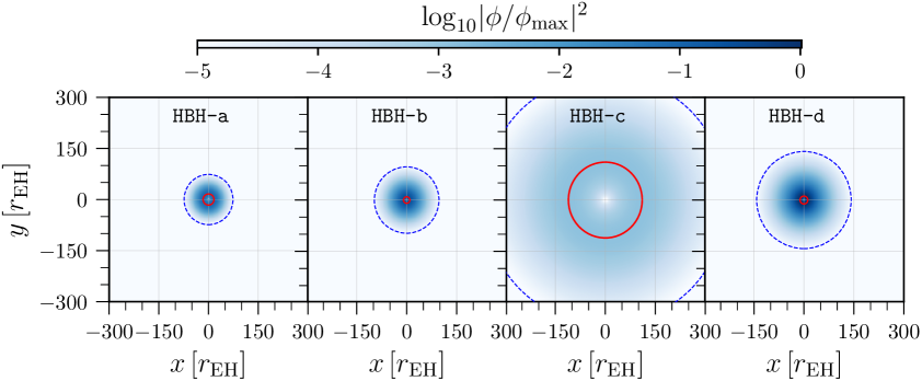
Figure 1: Two-dimensional distribution in the equatorial plane of the ultralight scalar hair density around the black hole (the three-dimensional morphology is that of a torus of scalar hair). The red circles show the location of the maximum amplitude, $\phi_{\rm max}$.

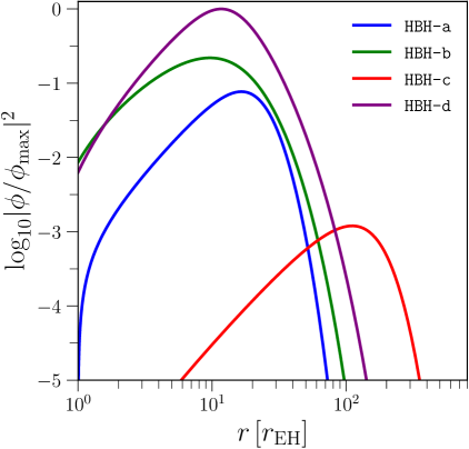
Figure 2: One-dimensional radial profiles of normalised scalar field amplitude, where $\phi_{\rm max}=3.2\times 10^{-1}$ is the maximum amplitude for model HBH-d.

The complex scalar field $\Psi=\Psi^{R}+i\Psi^{I}$, where $\Psi^{R}$ is its real part and $\Psi^{I}$ the imaginary one, respectively, is assumed to be minimally coupled to gravity. In this way, the Einstein–Klein-Gordon (EKG) evolution equations can be obtained by performing the variation of the action with respect to the metric and the complex scalar field. The action ${\cal S}$ and the energy-momentum tensor $T_{\sigma\lambda}$ of this system can be written as follows

$${\cal S} = \int d^{4}x\sqrt{-g}\left[\frac{R}{16\pi}-\frac{1}{2}g^{\sigma\lambda}(\partial_{\sigma}\Psi^{*}\partial_{\lambda}\Psi+\partial_{\sigma}\Psi\partial_{\lambda}\Psi^{*})\right.$$ (2.5)

$$\left.-\mu^{2}\Psi^{*}\Psi\right]\,,$$

$$T_{\sigma\lambda} := \partial_{\sigma}\Psi^{*}\partial_{\lambda}\Psi+\partial_{\sigma}\Psi\partial_{\lambda}\Psi^{*}$$ (2.6)

$$- g_{\sigma\lambda}\left[\frac{1}{2}g^{\gamma\delta}\left(\partial_{\gamma}\Psi^{*}\partial_{\delta}\Psi+\partial_{\gamma}\Psi\partial_{\delta}\Psi^{*}\right)+\mu^{2}\Psi^{*}\Psi\right]\,,$$

where $\Psi^{*}$ is the complex conjugate of $\Psi$, $g$ is the determinant associated with the components of the 4-metric $g_{\sigma\lambda}$, $R$ is the Ricci scalar, and $\mu$ is the mass of the scalar field.

The HBH solutions of the EKG equations employed in our numerical simulations are the same as in [72, 73, 76]. Specifically, we consider four illustrative solutions for hairy black holes. The corresponding scalar field masses and angular momenta are in the range $M_{\phi}\in[0.022,0.957]$ and $J_{\phi}\in[0.022,0.848]$, where the physical quantities are displayed in units of the scalar field mass $\mu$. Some relevant physical parameters of the HBHs used in our simulations are summarized in Tab. 1. As it can be seen from this table, the relative contribution of the scalar field to the mass and angular momentum is much higher for the last solutions (HBH-c,d), which are therefore hairier, whereas the first ones (HBH-a,b) are closer to Kerr. It is worth mentioning that in this work we focus on the impact of changing $M_{\phi}/M_{\rm BH}$ rather than studying the other degrees of freedom of the problem, such as the spin of the black hole or the adiabatic index of the gas. The impact of these different parameters will be the subject of future studies.

The numerical domain employed to construct the HBH solutions is $r\in[1.1\,r_{\rm EH},200\,M_{\rm BH}]$ and $\theta\in[0,\pi]$ (see also Sec. 4 for a description of the hydrodynamical grid). Additionally, since the numerical simulations of BHL accretion will be performed in the equatorial plane, $\theta=\pi/2$, we specialize the HBH solutions to this plane. Figure 1 shows the two-dimensional morphology of the normalized scalar field around the black hole (left panels, in Cartesian coordinates), where the red circle marks the location of the maximum amplitude of the scalar field. Correspondingly, Fig. 2 reports the radial distribution of the normalized scalar field amplitude. In each solution, the scalar field has a different mass, angular velocity, strength, and distribution in order to have a self-consistent solution, satisfying the constraints of the EKG system.

3 Problem setup

The general relativistic hydrodynamics equations in the $3+1$ spacetime decomposition are written in a conservative form following the Valencia formulation [84]

$$\partial_{t}(\sqrt{\tilde{\gamma}}\,\boldsymbol{U})+\partial_{i}(\sqrt{\tilde{\gamma}}\,\boldsymbol{F}^{i})=\sqrt{\tilde{\gamma}}\,\boldsymbol{S}\,,$$ (3.1)

where for the equatorial case $i,j=r,\phi$, and the conserved variables $\boldsymbol{U}$ and fluxes $\boldsymbol{F}^{i}$ are respectively

$$\boldsymbol{U}=\left[\begin{array}[]{c}D\\ S_{j}\\ \tau\end{array}\right]\,,\ \qquad\boldsymbol{F}^{i}=\left[\begin{array}[]{c}\mathcal{V}^{i}D\\ \alpha W^{i}_{j}-\beta^{i}S_{j}\\ \alpha(S^{i}-v^{i}D)-\beta^{i}\tau\end{array}\right]\,,$$ (3.8)

where $\mathcal{V}^{i}:=\alpha v^{i}-\beta^{i}$ are the components of the transport velocity, and $W^{ij}:=S^{i}v^{j}+p\tilde{\gamma}^{ij}$ are the spatial components of the stress-energy tensor, $\alpha$, $\tilde{\gamma}$, and $\beta^{i}$ are the lapse function, the determinant of the 3-metric, and the shift vector components, respectively. The conserved quantities in the Eulerian frame are given by the following relations

$$D := \Gamma\rho,$$ (3.9)

$$S_{j} := \rho h\Gamma^{2}v_{j},$$ (3.10)

$$\tau := \rho h\Gamma^{2}-p-D,$$ (3.11)

where $\Gamma:=\alpha u^{0}$ is the Lorentz factor with respect to the Eulerian observer, $\rho$ is the rest-mass density, $h=1+\epsilon+p/\rho$ is the specific enthalpy, $p$ is the fluid pressure and $\epsilon$ the specific internal energy. It is worth mentioning that the fluid corresponds to a perfect one which we model with an ideal gas equation of state. Finally, the sources $\boldsymbol{S}$ in the right-hand-side of equation (3.1) are

$$\boldsymbol{S}=\left[\begin{array}[]{c}0\\ \frac{1}{2}\alpha W^{ik}\partial_{j}\tilde{\gamma}_{ik}+S_{i}\partial_{j}\beta^{i}-U\partial_{j}\alpha\\ \frac{1}{2}W^{ik}\beta^{j}\partial_{j}\tilde{\gamma}_{ik}+W_{i}^{j}\partial_{j}\beta^{i}-S^{j}\partial_{j}\alpha\end{array}\right]\,.$$ (3.15)

A well-known feature of the above equations is that after every time step it is mandatory to compute the primitive variables ($\rho,\,\Gamma v^{i},\,p$) in order to compute the numerical fluxes, through some implicit procedure. In this work, we are using the method “1DW" to recover the Lorentz factor in order to avoid superluminal velocities, as prescribed in the BHAC code [85, 86, 87].

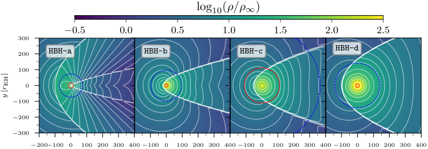
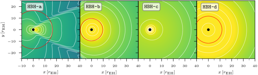
Figure 3: Two-dimensional distributions (colormap) and isocontours (grey lines) of the rest-mass density normalized by its initial value $\rho_{\infty}$ and at the end of the numerical evolution $t=10000\,M_{\rm BH}$ for the four HBHs considered here. Red solid circles mark the location of the maximum scalar field $\phi_{\rm max}$, while the blue dashed circles mark the outer edge of the torus of scalar hair so that the two circles provide a view of the torus size. The top and bottom rows report respectively large- and small-scales views of portions of the computational domain so that the different parts of the dynamics can be appreciated.

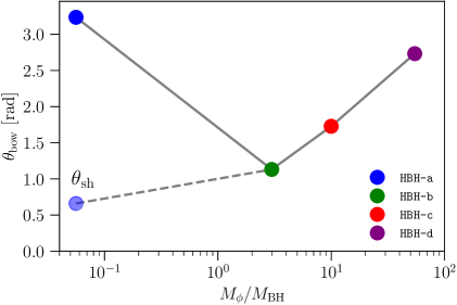
Figure 4: Bow-shock opening angle $\theta_{\rm bow}$ shown as a function the relative weight of the scalar field via the mass ratio $M_{\phi}/M_{\rm BH}$ for the four HBHs considered. In the case of model HBH-a we also report the (downstream) shock-cone opening angle $\theta_{\rm sh}$ that shows a monotonic behaviour in terms of $M_{\phi}/M_{\rm BH}$.

As customary in these simulations, the black hole is placed at the center of the computational domain, which is then filled by accreting gas modeled has having a uniform density and moving along the positive $x$-direction. Since the coordinates used in the code are spherical, the velocity-field components are

$$v^{r} = \phantom{-}v_{\infty}{\cal H}_{1}\cos\varphi+v_{\infty}{\cal H}_{2}\sin\varphi\,,$$ (3.16)

$$v^{\varphi} = -v_{\infty}{\cal H}_{3}\sin\varphi+v_{\infty}{\cal H}_{4}\cos\varphi\,,$$ (3.17)

where ${\cal H}_{i}$ are functions written in terms of the metric components and $v_{\infty}$ is the asymptotic velocity of the fluid (see Refs. [38, 40, 42, 88, 48] for more details). On the other hand, the pressure of the gas is constructed from the definition of the sound speed for an ideal gas, that is, $c^{2}_{\rm s}=p\gamma(\gamma-1)/[p\gamma-\rho(\gamma-1)]$ [32]. Based on this, and using the ideal-gas equation of state $p=\rho\epsilon(\gamma-1)$, the initial pressure of the gas is set to

$$p_{\rm ini}=\frac{c^{2}_{\rm s,\infty}\rho_{\infty}(\gamma-1)}{\gamma(\gamma-1)-c^{2}_{\rm s,\infty}\gamma}\,,$$ (3.18)

where the adiabatic index $\gamma$, the speed of sound at infinity $c_{\rm s,\infty}$, the asymptotic rest-mass density $\rho_{\infty}$ and the asymptotic velocity $v_{\infty}$ are free parameters. Specifically, in this work we use $\gamma=5/3$, $\rho_{\infty}=10^{-8}$, $c_{\rm s,\infty}=0.1$ and $v_{\infty}=0.5$. As a result, the gas is supersonic, with Newtonian Mach number at infinity ${\cal M}:=v_{\infty}/c_{\rm s,\infty}=5$.

All simulations reported in this work were carried out in two spatial dimensions using the BHAC code [85, 86, 87], employing spherical coordinates $(r,\varphi)$ on the equatorial plane and a logarithmic radial coordinate $R:={\rm log}(r)$. The numerical grid over which the hydrodynamical equations are solved covers the spherical-polar coordinates domain $r/r_{\rm EH}\in[1.1,1000]$ and $\varphi\in[0,2\pi]$; hence, the hydrodynamical grid always includes the grid over which the HBH solutions are computed. In the intermediate region, e.g., for $200\lesssim r/M_{\rm BH}\lesssim 1000$, we simply employ the Kerr solution in Boyer-Lindquist coordinates, since the differences of the HBH solutions are very small at these distances. In the left hemisphere (i.e., for $x<0$) we inject gas with constant velocity and density at the outer radius, using the same prescription as the initial conditions. On the other hand, in the right hemisphere (i.e., for $x\geq 0$), we impose an outflow boundary at the inner and outer radii for $x>0$. Periodic boundary conditions are imposed in the $\varphi$ direction. For the simulations we use an adaptive mesh refinement algorithm [89], with three levels of refinement, where the coarse grid resolution corresponds to $\Delta R=3.56\times 10^{-3}$ for the logarithmic radial coordinate and $\Delta\varphi/\pi=3.9\times 10^{-3}$ for the angular one. Additionally, we use the finite-volume method to solve the general relativistic hydrodynamics equations (3.1), with the particular choices of the HLLE (Harten, Lax, van Leer, and Einfeldt) flux formula [90, 91] and the minmod slope limiter to compute the fluxes and reconstruct the primitive variables at cell interfaces, respectively [32]. The time update in all simulations is performed using a third-order Runge-Kutta time integrator.

4 Results

The morphology of the accreting gas after the simulations have reached a steady-state is shown in the different panels of Fig. 3 for all HBHs of our sample. The figure displays with a colormap and isocontours the two-dimensional distribution of the rest-mass density at $t=10000\,M_{\rm BH}$ and normalised to its asymptotic value. The morphology of the various configurations exhibits the typical behavior of relativistic BHL accretion onto a moving black hole. More specifically, and as first learnt in simulations involving Kerr black holes (see, e.g., Refs. [38, 39, 40, 47, 33]), when a supersonic gas moves past an HBH, a shock-cone appears downstream, in the proximity of the black hole. This shock-cone is clearly visible not only in Fig. 3, but also in the left panels of Fig. 5, which displays instead the distribution of the Mach number. Each panel in Fig. 3 reports with red solid circles the location of the maximum scalar field $\phi_{\rm max}$, while with blue dashed circles the outer edge of the torus of scalar hair, which is defined as the radius where the normalized scalar field density is five orders of magnitudes smaller than $\phi_{\rm max}$. Hence the region between the two circles can be taken as an indication of the size of the torus of scalar hair.

Despite these common features, each HBH solution interacts with the inflowing plasma developing different gas patterns. Such differences can be observed in the shock-cones temperature profiles, velocity fields (see streamlines in Fig. 5), and opening angles $\theta_{\rm sh}$. The latter are plotted in Fig. 4 and are measured as follows. We compute the normalized rest-mass density as a function of the $\varphi$ coordinate at $r=200\,r_{\rm EH}$ and then mark the opening angle as the angle at which the density gradient in the angular direction, $\partial_{\varphi}\rho$, diverges; the opening angles for the different HBH models are listed in Table 2. As shown in Fig. 4 and reported in Table 2, the opening angle overall increases as the “hairiness" of the black hole is also increased. In the case of model HBH-a the figure also reports the (downstream) shock-cone opening angle $\theta_{\rm sh}$ that shows a monotonic behaviour in terms of $M_{\phi}/M_{\rm BH}$. An intuitive explanation of this behaviour comes when considering that as the contribution in mass and angular momentum of the scalar hair becomes comparable to that of the black hole, the “local” curvature will be less severely modified by the black hole and hence the impact of the black hole on the incoming flow, namely the shock-cone, will be smaller.

The HBH solution HBH-a corresponds to the least hairy black hole of our set and is thus more Kerr-like. In this case, two shock fronts develop in the flow: first, a broad and strong bow-shock appears upstream of the black hole with an opening angle $\varphi_{\rm bow}\sim\pi~{}{\rm rad}$; second, a narrow and weak shock-cone forms downstream, similar to what is observed for pure Kerr black holes. When considering more hairy black holes, on the other hand, the trailing shock-cone starts enveloping entirely the black hole as the amount of scalar hair increases (see the transition from model HBH-b to model HBH-d), transforming itself into a leading bow-shock. The explanation for this different flow morphology has to be found again in the fact that the curvature, especially near the black hole, becomes less severe as the strength of the scalar field is increased, so that the impact of the black hole on the incoming flow is less and less marked. As a result, the second downstream shock weakens up to disappearing, as can be seen in the various panels of Fig. 3.

Additionally, the different HBH solutions explored in our simulations have different accretion properties, which can be characterized in terms of several quantities. The first one is the so-called accretion radius, defined as [32]

$$r_{\rm acc}:=\frac{M_{\rm BH}}{c^{2}_{s,\infty}+v^{2}_{\infty}}\,,$$ (4.1)

and which marks the transition of the flow from subsonic to supersonic velocities. The accretion radius can also be interpreted as marking the spherical region within which gravity dominates and so it is expected to decrease as the amount of the scalar hair is increased [cf., Table 2]. Other important quantities are the accretion rates of rest-mass $\dot{M}$ and linear momentum $\dot{P}^{i}$, which are computed as [34]

$$\dot{M} := \int_{0}^{2\pi}\alpha\sqrt{\tilde{\gamma}}D(v^{r}-\beta^{r}/\alpha)d\varphi\,,$$ (4.2)

$$\dot{P}^{r} := -\int_{\partial V}\alpha\sqrt{\tilde{\gamma}}T^{rj}d\Sigma_{j}+\int_{V}\alpha\sqrt{\tilde{\gamma}}S^{r}dV\,,$$ (4.3)

where the inward fluxes are measured at the event horizon of each HBH solution. The volume and surface integrals were calculated at volume $V$ and surface $\partial V$ defined by the sphere with radius $2r_{\rm EH}$. In the case of spherical accretion onto nonrotating black holes, $\dot{M}$ and $\dot{P}^{i}$ can be computed analytically to be [34, 32]

$$\dot{M}_{\rm ref} = 4\pi\lambda\rho_{\infty}M_{\rm BH}^{1/2}r^{3/2}_{\rm acc}\,,$$ (4.4)

$$\dot{P}_{\rm ref} = \dot{M}_{\rm ref}\frac{v_{\infty}}{\sqrt{1-v^{2}_{\infty}}}\,,$$ (4.5)

where

$$\lambda:=\left(\frac{1}{2}\right)^{(\gamma+1)/(2(\gamma-1))}\left(\frac{5-3\gamma}{4}\right)^{-(5-3\gamma)/(2(\gamma-1))}\,,$$ (4.6)

with $\lambda\sim 1/4$ when $\gamma=5/3$. We will use expressions (4.4) and (4.5) as reference values against which we normalize the accretion rates in our set of HBH spacetimes and report them in Table 2.

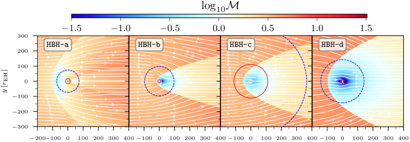
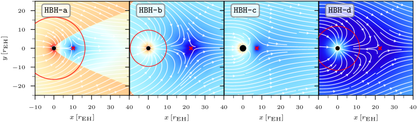
Figure 5: The same as in Fig. 3 but for the Newtonian Mach number ${\cal M}$. In addition, shown with white lines are the fluid streamlines, while a red cross is used to mark the position of the stagnation point.

However, before discussing such quantitative properties of the accretion flow, it is useful to return to the more general morphological properties. To this scope, we note that the motion of the gas can be best followed through the streamlines plotted in white in the various panels of Fig. 5, which also reports with a colormap the Mach number in the steady-state configuration of the flow at $t=10000\,M$. Starting from a constant velocity flow in the positive $x$-direction with $v_{\infty}=0.5$ (note that the streamlines are parallel), we observe that the bulk of the flow close to the black hole is accreted, while the flow further away is hardly perturbed by the presence of the black hole and escapes in its motion. The gas that is captured experiences a sharp transition from a supersonic flow to a subsonic one as it is braked by the black hole and subsequently accreted. The Mach number reaches particularly small values for solutions where the mass and spin of the scalar field dominate over those of the black hole, namely for model HBH-d. Interestingly, as the scalar hair of the black hole increases, the velocity distribution becomes more and more spherically symmetric, as can be appreciated when contrasting models HBH-a and HBH-d.

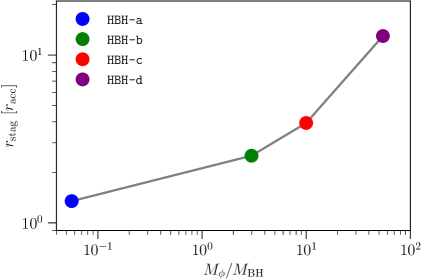
Figure 6: Radial position of the stagnation point in units of the accretion radius and shown as a function the relative weight of the scalar field via the mass ratio $M_{\phi}/M_{\rm BH}$.

Figure 5 also reveals that there are streamlines converging into a single point downstream of the black hole and inside the shock-cone. At such a point, which is identified in the figure with a red cross and is commonly referred to as the “stagnation point” $r_{\rm stag}$, the velocity is zero and the fluid is in unstable equilibrium, so that any perturbation can either push the fluid into the black hole or away from it, in the downstream flow. Figure 6 reports the location of the stagnation point as a function of the mass ratio $M_{\phi}/M_{\rm BH}$ for our four HBH models when expressed in terms of the accretion radius $r_{\rm acc}$. Also in this case, it is apparent that the hairier the solution the larger the stagnation radius and hence the more extended the low-velocity (subsonic) region. This is also clear in the various panels of Fig. 5, where different shades in the colormap characterize models HBH-a and HBH-d. As for other quantities, Table 2 reports the mean value and the standard deviation of $r_{\rm stag}$ for every HBH of our sample, measured from the saturation time (defined below) up to the end of each numerical simulation.

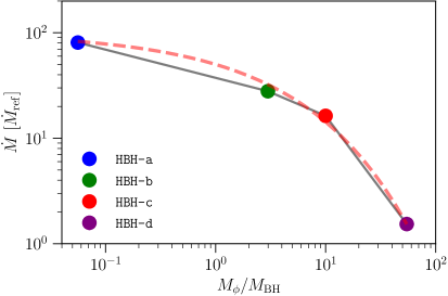
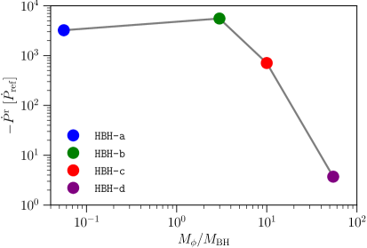
Figure 7: Accretion rates of rest-mass (top panel) and of the radial momentum (bottom panel); both quantities are normalized by the corresponding quantities ($\dot{M}_{\rm ref}$, $\dot{P}_{\rm ref}$) in the case of spherical accretion onto a nonrotating black hole and refer to values attained when the flow has reached a steady-state. The red dashed line shows the fit given by expression (4.7).

In Fig. 7 we show the rest-mass and radial-momentum accretion rates normalized by their reference values, $\dot{M}_{\rm ref}$ and $\dot{P}_{\rm ref}$, as a function of the mass ratio $M_{\phi}/M_{\rm BH}$. The values reported correspond to the steady-state flow solution after the equilibrium time $\tau_{\rm eq}$ has been achieved. The latter is defined as the time when the accretion process starts reaching a stationary state (i.e., when ${\ddot{M}}\leq 10^{-4}/M$) and clearly varies with the amount of scalar hair, becoming significantly smaller as the amount of scalar field is increased (see Table 2). Note that rest-mass accretion rates decrease for hairier solutions, which have a shallower gravitational potential and thus reduce the accretion efficiency. However, HBHs have quite generically mass-accretion rates that are larger than their corresponding hairless counterparts. Similarly, the radial-momentum accretion rate also decreases from model HBH-a to model HBH-d, which is consistent with the fact that the amount of matter able to transfer linear momentum decreases with the increase of scalar field. Also for this quantity, HBHs have quite generically momentum-accretion rates that are three or even four orders of magnitude larger than pure Kerr black holes.

Once the system reaches a steady-state it is possible to compute semi-analytical relations for the mass accretion rates as a function of the scalar-field-to-black-hole mass ratio. Fits to our numerical results in the steady-state regime are given by

$$\log_{10}\left(\frac{\dot{M}}{\dot{M}_{\rm ref}}\right) = 2-0.3\left(\frac{M_{\phi}}{M_{\rm BH}}\right)^{0.45}\,.$$ (4.7)

The expression above, which is shown in the top panel of Fig. 7 with a dashed line, can be used to explore, for instance, progenitor initial masses and spins of binary black hole gravitational-wave events [92, 93, 94] when accounting for the possible effects a surrounding ultralight scalar field might have. Efforts along these lines, albeit without the inclusion of bosonic clouds, have been reported recently in connection with the nature of the transient event GW190521. Using Newtonian [10, 95] and relativistic accretion models [33, 9] three possible scenarios for the origin of the progenitor have been discussed, namely involving primordial black holes, stellar-mass black holes formed by direct collapse, and intermediate-mass black holes resulting from the collapse of Pop III stars. Taking into account the potential contribution of ultralight scalar field dark matter is relevant to further assess those models.

Model	$r_{\rm acc}$	$\dot{M}_{\rm ref}$	$\dot{P}_{\rm ref}$	$\langle\dot{M}\rangle$	$\langle\dot{P}^{r}\rangle$	$r_{\rm stag}$	$\theta_{\rm bow}$	$\tau_{\rm eq}$
	$[M_{\rm BH}]$			$[\dot{M}_{\rm ref}]$	$[\dot{P}_{\rm ref}]$	$[r_{\rm acc}]$	$[{\rm rad}]$	$[M_{\rm ADM}]$
HBH-a	$1.51$	$3.66\times 10^{-8}$	$2.11\times 10^{-8}$	$9.01\times 10^{1}$	$-3.59\times 10^{3}$	$1.35$	$3.24$	$88$
HBH-b	$0.90$	$1.30\times 10^{-8}$	$7.50\times 10^{-9}$	$4.43\times 10^{2}$	$-8.79\times 10^{4}$	$2.51$	$1.13$	$24$
HBH-c	$0.19$	$5.70\times 10^{-10}$	$3.29\times 10^{-10}$	$1.97\times 10^{3}$	$-8.55\times 10^{4}$	$3.94$	$1.73$	$5$
HBH-d	$0.07$	$7.30\times 10^{-11}$	$4.21\times 10^{-11}$	$4.74\times 10^{3}$	$-1.15\times 10^{4}$	$12.99$	$2.73$	$6$

Table 2: Summary of the quantities measured numerically results for all of the HBHs explored in this work. Reported are the accretion radius $r_{\rm acc}$, the rest-mass and radial-momentum accretion rates $\dot{M}$ and $\dot{P}^{r}$ expressed in terms of the corresponding quantities $\dot{M}_{\rm ref}$ and $\dot{P}_{\rm ref}$ for spherical accretion onto a nonrotating black hole, the position of the stagnation $r_{\rm stag}$ point in $r_{\rm acc}$ units, the opening angle of the bow-shock $\theta_{\rm bow}$, and the equilibrium time $\tau_{\rm eq}$ needed for the flow to reach steady-state.

5 Application to QPOs in Sgr A* and microquasars

As an astrophysical application of the results on BHL-accretion past HBHs reported above and to find potential associations with the QPOs observed in Sgr A* and in microquasars, we consider the frequency spectrum of the fluid oscillations that arise within the shock-cone and that are related to the stagnation point. We recall that the association of QPOs with oscillations of the shock-cone in the downstream part of a BHL flow was first reported in Ref. [39]. In essence, it was noted that the shock-cone acts as a cavity trapping pressure perturbations and exciting specific $p$-modes (see Ref. [96, 97, 98] for a similar process taking place in accretion disks around black holes in general relativity). For black-hole spacetimes without scalar hair, it was found that the frequencies of these modes depend on the black-hole spin and on the properties of the flow, and scale linearly with the inverse of the black-hole mass [39]. Here, we investigate how much the presence of the scalar field in our HBH spacetimes modifies the mode frequencies of the shock-cone vibrations and the additional resonant cavities that emerge because of the presence of a scalar field.

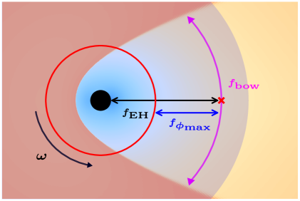
Figure 8: Schematic diagram of the resonant cavities produced in a BHL flow onto a HBH where a $p$-mode can be trapped. The first cavity is formed between the stagnation point (red cross) and the event horizon, with an associated frequency $f_{\rm EH}$ (black arrows). The second one is between the stagnation point and the position of the maximum of the scalar field amplitude (red solid line) with frequency in this cavity is $f_{\phi_{\rm max}}$ (blue arrows), while the scalar field orbital frequency is $\omega$. The third cavity is that enclosed by the bow-shock where $p$-modes travel transversally to the shock-cone with frequency $f_{\rm bow}$ (magenta arrows). Finally, in the case of model HBH-a (and of a Kerr black hole) another cavity is present in the downstream shock-cone with $p$-modes trapped at frequency $f_{\rm sh}$. The color map shows the rest-mass density of the gas and the ultralight scalar hair distribution (grey-shaded area).

Figure 8 provides a schematic diagram of the possible resonant cavities that can be formed around the stagnation point, and where pressure perturbations can propagate a distance $L$ with velocity $c_{s}$. To cover all of these possibilities, we define a generic resonant $p$-mode frequency as $f_{i}:=c_{s,i}/L_{i}$, where $i$ is not an integer and is used to indicate the different resonant cavities that can be produced in the flow (see Table 3). The first cavity is then formed between the stagnation point (red cross) and the event horizon, with an associated frequency $f_{\rm EH}$ (black arrows). The second one is between the stagnation point and the position of the maximum of the scalar field amplitude (red solid line) whose rotation frequency is $\omega$; the $p$-mode oscillations in this cavity have a frequency $f_{\phi_{\rm max}}$ (blue arrows). The third cavity is that enclosed by the upstream bow-shock and in this region sound waves travel transversally to the shock with frequency $f_{\rm bow}$ (red arrows). Finally, in the case of model HBH-a (and of a Kerr black hole) another cavity is present in the downstream shock-cone with $p$-modes trapped at frequency $f_{\rm sh}$.

The resonant frequencies expected on the basis of the measured values of $L_{i}$ and $c_{s,i}$ are reported for each HBH in Table 3 and in units of $1/M_{\rm ADM}$. Note that the frequencies at the shock-cone are different for each HBH model because, on the one hand, the opening angle increases with the mass ratio $M_{\rm SF}/M_{\rm BH}$ (see Fig. 4) and, on the other hand, the sound speed also changes when the gas moves from supersonic to subsonic velocities. Similarly, the frequency $f_{\rm EH}$ is also different for each HBH since the position of the stagnation point changes as a function of $M_{\phi}/M_{\rm BH}$ (see Fig. 6).

The predictions for the expected frequencies can be compared with the power spectral density (PSD) as obtained after performing a Fourier transform of the rest-mass density measured at the stagnation point of each HBH model. Furthermore, to increase the robustness of our results, we also compute the PSDs in ten detectors located around the stagnation point and compute the mean and the corresponding standard deviation of the measured frequencies. Figure 9 shows the mean PSD (colored solid lines) and the standard deviation for each HBH spacetime (colored shaded regions). In addition, the grey line and shaded region in the top panel for model HBH-a corresponds to a Kerr black hole with spin $a_{\star}=15/16\ (\Omega_{\rm EH}=0.35)$, which we use as a reference

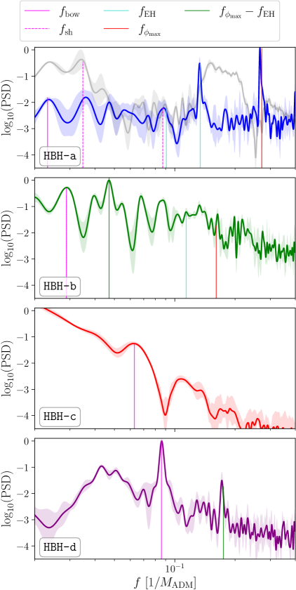
Figure 9: Power spectral densities (PSD) of the rest-mass density evolution measured at the stagnation point. Each panel refers to a different HBH, with colored solid lines showing the PSDs and the corresponding shaded regions indicating the standard deviation. The grey line and area reports the PSD for a Kerr black hole with spin $a_{\star}=15/16$. The expected values of the representative frequencies are reported with colored vertical lines (see also Table 3).

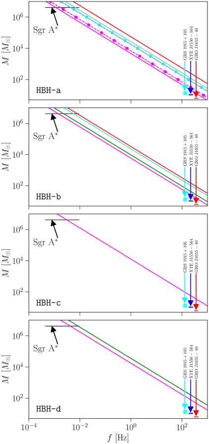
Figure 10: The four panels report the QPO frequencies for the four HBHs considered and black-hole masses in the range $M/M_{\odot}\in[1,\,10^{7}]$. The colored lines correspond to the vertical lines shown in Fig. 9, while the filled markers in the top panel refer to the QPO frequencies for a Kerr black hole. Also reported are the observed QPO frequencies for Sgr A* $(f/{\rm mHz}\in{\rm[0.434,\,10]})$, GRO J1655-40 $(f/{\rm mHz}\in{\rm[300,\,450]}$), XTE J1550-564 at 184 Hz and 276 Hz, and for GRS 1915+105 $(f/{\rm mHz}\in{\rm[113,\,168]})$.

For all models, we identify several peaks in the spectrum and use vertical lines to report the predicted resonant frequencies described above. Starting from the reference pure-Kerr black hole, it is possible to recognize in the PSD the low-frequency $p$-mode in the shock-cone $f_{\rm sh}$ (together with overtones at $2f_{\rm sh}$, $3f_{\rm sh}$, and $5f_{\rm sh}$) and the high-frequency resonance between the accretion radius and the event horizon $f_{\rm EH}$. When passing to the HBH solutions, it is possible to recognise for model HBH-a the peaks corresponding to the $p$-mode frequencies in the cavity produced by the (upstream) bow-shock $f_{\rm bow}$, the mode at $f_{\rm sh}$ trapped in the (downstream) shock-cone (present only for model HBH-a), the mode at $f_{\rm EH}$ in the cavity between the event horizon and the stagnation point, and the mode at $f_{\phi_{\rm max}}$ in the cavity between the stagnation point and the maximum of the scalar field. For model HBH-b we can clearly identify the main peaks with frequencies at $f_{\rm bow}$, $f_{\rm EH}$, and $f_{\phi_{\rm max}}$, but also some minor peaks which are related to combinations of the main frequencies, e.g., $(f_{\rm bow}+f_{\rm EH})/2$, $3f_{\rm bow}$, and $(f_{\phi_{\rm max}}+f_{\rm EH})/2$ (not reported in the panel). On the other hand, for model HBH-c we can only identify clearly the main low-frequency mode at $f_{\rm bow}$, while subdominant peaks appear at the first two overtones, $2f_{\rm bow}$ and $3f_{\rm bow}$. Finally, for model HBH-d the two dominant peaks coincide with the trapped $p$-mode at $f_{\rm bow}$ and with the combination of frequencies $f_{\phi_{\rm max}}-f_{\rm EH}$; this model has the largest shock-cone opening angle and the observed low-frequency peak corresponds interestingly to $f_{\rm bow}/2$.

${\rm Model}$	$f_{\rm bow}$	$f_{\rm sh}$	$f_{\rm EH}$	$f_{\phi_{\rm max}}$
HBH-a	$0.023$	$0.087$	$0.134$	$0.272$
HBH-b	$0.029$	$-$	$0.114$	$0.161$
HBH-c	$0.063$	$-$	$0.554$	$0.020$
HBH-d	$0.086$	$-$	$0.343$	$0.518$
Kerr	$-$	$0.035$	$0.091$	$-$

Table 3: Resonance frequencies produced in the various cavities illustrated in Fig. 8. The last row reports the frequencies for a Kerr black hole with $a_{\star}=15/16$; all frequencies are in units of $1/M_{\rm ADM}$.

Overall, the discussion above shows that the presence of and ultralight scalar-field does leave an imprint in the QPO frequencies of the accreting HBH. Since each model has different frequencies, those could be used to potentially distinguish between a black hole with a light amount of hair (Kerr-like) from a hairier black hole (boson-star-like). Going further, and notwithstanding the speculative nature of these considerations, we could compare the resonant frequencies of our HBH models with observational measurements of QPO frequencies in actual astronomical sources to see the role scalar fields might play to fit the data. To do so, we use the QPOs observed in the X-ray lightcurve of Sgr A* [99] and of three microquasars, namely GRO J1655-40, XTE J1550-564, and GRS 1915+105 [101]. Figure 10 shows the main QPO frequencies we identify in our models, using the same color coding as in Fig. 9, as a function of the black hole mass.

Unfortunately, the outcome of this comparison is not conclusive for the case of Sgr A* since the range of QPO frequencies is so large that all of our HBH models can explain the observed frequencies as due to either to $p$-mode oscillations trapped in the bow-shock or to radial oscillations between the stagnation point and the event horizon. We should also note that the QPOs of a Kerr black hole are also compatible with the observed frequencies, e.g., for a $M\sim 10\,M_{\odot}$ Kerr black hole the frequency is $\sim 100\,$Hz, (see also the results from [39]). On the other hand, for the three microquasar sources considered, no HBH or Kerr black hole can explain the observed QPO frequencies. The only exception is model HBH-a, for which the low-frequency QPO $f_{\rm bow}$ is low enough to be close to the frequency observed for GRO J1655-40.

6 Summary

We have studied relativistic BHL accretion onto an illustrative sample of the hairy black-hole solutions reported by [72, 73]. The hair has been assumed to be composed of an ultralight, complex scalar field, minimally coupled to Einstein’s gravity. We have considered four solutions, describing HBHs with different amounts of hair, ranging from Kerr-like to boson star-like. Through numerical simulations using the BHAC code, we have explored the dynamics and flow morphology of a $\gamma=5/3$ ideal gas moving supersonically past the four HBHs and searched for signatures in the observable quantities that may provide evidence of a deviation from the dynamics expected from Kerr back holes.

The simulations have revealed that the morphology of the flow past HBHs is fairly similar to that found when studying relativistic BHL accretion onto a Kerr black hole [38, 39, 40, 47, 33]. More specifically, all simulations lead to a steady-state morphology characterized by the formation of a bow-shock cone in the upstream part of the flow, where the gas becomes subsonic, along with the presence of a stagnation point where the flow velocity vanishes. However, as the amount of hair around the black hole increases, so does the opening angle of the bow-shock-cone, while the stagnation point moves further downstream and away from the black hole. Both of these effects can be clearly associated to the presence of the scalar field that distorts the spacetime near the black hole and reduces locally the curvature. The weakening of the gravitational influence of the black hole as a result of the increase of the scalar-hair strength has an additional manifestation in the so-called shock-cone that develops for BHL onto black holes in general relativity and hence without scalar hair [38, 39]. This very specific signature that is very robust in hairless black holes is recovered in our analysis only in the less hairy of the HBHs (HBH-a) and is absent (or is very weak) as the amount of scalar hair is increased and the overall compactness of the spacetime decreased (the gravitational well is distributed over a larger volume).

Our simulations have also allowed to compute the rest-mass and linear-momentum accretion rates, finding that they attain stationary values after a (model-dependent) equilibration time is reached. A semi-analytical fit for the rest-mass accretion rate in terms of the mass ratio $M_{\phi}/M_{\rm BH}$ has been found, which could potentially be used to analyze different black-hole formation scenarios in the presence of ultralight scalar-field dark matter.

Finally, we have explored how the modifications in the spacetime affect one of the most intriguing aspects of BHL accretion onto black holes, namely the presence of quasi-periodic oscillations corresponding to resonant waves trapped in the cavities that are produced in the flow. The existence of such QPOs, which was first pointed out in Ref. [39] in the case of a Kerr black hole, has been confirmed also in the case of the HBHs considered here, where they appear with a much richer phenomenology. This is because BHL accretion onto HBHs leads to the formation of a number of resonant cavities, namely: in the upstream bow-shock and, for weak scalar fields, in the downstream shock-cone, but also between the stagnation point and the event horizon, and between the stagnation point and the position of the maximum of the scalar field amplitude. We have computed such frequencies and have compared them with the QPOs observed in the X-ray light curve of Sgr A* and three microquasars. Although the results of this comparison are not conclusive, possibly because the galactic centre is a highly complex and dynamical system with extremely low accretion rates and with inflow geometries that are not necessarily those of classical disc accretion, we argue that further work along these lines and the measurement of QPOs in other supermassive black holes might help establish a possible observational fingerprint for ultralight scalar field dark matter.

In summary, the results presented here provide a first quantitative description of the BHL gas dynamics past HBHs, where the gravitational field is produced by the combined presence of a black hole and a scalar hair. In an astrophysical context, this study can help associate specific features in the evolution of the gas to different system components, i.e., either the black hole, the scalar field, or the combination of the two through their gravitational interaction.

References

- Event Horizon Telescope Collaboration et al. [2019] Event Horizon Telescope Collaboration, K. Akiyama, A. Alberdi, W. Alef, K. Asada, R. Azulay, A.-K. Baczko, D. Ball, M. Baloković, J. Barrett, et al., Astrophys. J. Lett. 875, L1 (2019).
- Event Horizon Telescope Collaboration et al. [2022] Event Horizon Telescope Collaboration, K. Akiyama, A. Alberdi, W. Alef, J. C. Algaba, R. Anantua, K. Asada, R. Azulay, U. Bach, A.-K. Baczko, et al., Astrophys. J. Lett. 930, L12 (2022).
- Remillard and McClintock [2006] R. A. Remillard and J. E. McClintock, Ann. Rev. Astron. Astroph. 44, 49 (2006), arXiv:astro-ph/0606352.
- Abbott et al. [2016] B. P. Abbott, R. Abbott, T. D. Abbott, M. R. Abernathy, F. Acernese, K. Ackley, C. Adams, T. Adams, P. Addesso, R. X. Adhikari, et al., Phys. Rev. Lett. 116, 061102 (2016), 1602.03837.
- Ferrarese and Ford [2005] L. Ferrarese and H. Ford, Space Science Reviews 116, 523 (2005), astro-ph/0411247.
- Kormendy and Ho [2013] J. Kormendy and L. C. Ho, Annual Review of Astronomy and Astrophysics 51, 511 (2013), 1304.7762.
- The LIGO Scientific Collaboration and the Virgo Collaboration [2020] The LIGO Scientific Collaboration and the Virgo Collaboration, Phys. Rev. Lett. 125, 101102 (2020), 2009.01075.
- Bustillo et al. [2021] J. C. Bustillo, N. Sanchis-Gual, A. Torres-Forné, J. A. Font, A. Vajpeyi, R. Smith, C. Herdeiro, E. Radu, and S. H. W. Leong, Phys. Rev. Lett. 126, 081101 (2021), 2009.05376.
- Cruz-Osorio et al. [2021] A. Cruz-Osorio, F. D. Lora-Clavijo, and C. Herdeiro, Journal of Cosmology and Astroparticle Physics 2021, arXiv:2101.01705 (2021), 2101.01705, URL https://doi.org/10.1088/1475-7516/2021/07/032.
- De Luca et al. [2021a] V. De Luca, V. Desjacques, G. Franciolini, P. Pani, and A. Riotto, Phys. Rev. Lett. 126, 051101 (2021a), 2009.01728.
- Shibata et al. [2021] M. Shibata, K. Kiuchi, S. Fujibayashi, and Y. Sekiguchi, Phys. Rev. D 103, 063037 (2021), 2101.05440.
- Gamba et al. [2022] R. Gamba, M. Breschi, G. Carullo, S. Albanesi, P. Rettegno, S. Bernuzzi, and A. Nagar, Nature Astronomy (2022), 2106.05575.
- Lightman and Shapiro [1977] A. P. Lightman and S. L. Shapiro, Astrophys. J. 211, 244 (1977).
- Begelman et al. [2006] M. C. Begelman, M. Volonteri, and M. J. Rees, Mon. Not. R. Astron. Soc. 370, 289 (2006), astro-ph/0602363.
- Volonteri [2010] M. Volonteri, Astronomy and Astrophysics Reviews 18, 279 (2010), 1003.4404.
- Hoyle and Lyttleton [1939] F. Hoyle and R. A. Lyttleton, in Proceedings of the Cambridge Philosophical Society (1939), vol. 35, p. 405.
- Bondi and Hoyle [1944] H. Bondi and F. Hoyle, Mon. Not. R. Astron. Soc. 104, 273 (1944).
- Bondi [1952] H. Bondi, Mon. Not. R. Astron. Soc. 112, 195 (1952).
- Hunt [1971] R. Hunt, Mon. Not. R. Astron. Soc. 154, 141 (1971).
- Matsuda et al. [1987] T. Matsuda, M. Inoue, and K. Sawada, Mon. Not. Roy. Astr. Soc. 226, 785 (1987).
- Fryxell and Taam [1988] B. A. Fryxell and R. E. Taam, Astrophys. J. 335, 862 (1988).
- Sawada et al. [1989] K. Sawada, T. Matsuda, U. Anzer, G. Boerner, and M. Livio, Astron. and Astrophys. 221, 263 (1989).
- Livio et al. [1991] M. Livio, N. Soker, T. Matsuda, and U. Anzer, Mon. Not. Roy. Astr. Soc. 253, 633 (1991).
- Ruffert and Melia [1994] M. Ruffert and F. Melia, Astron. Astrophys. 288, L29 (1994).
- Ruffert and Arnett [1994] M. Ruffert and D. Arnett, Astrophys. J. 427, 351 (1994).
- Ruffert [1997] M. Ruffert, Astron. Astrophys. 317, 793 (1997), arXiv:astro-ph/9605072.
- Foglizzo and Ruffert [1999] T. Foglizzo and M. Ruffert, Astron. Astrophys. 347, 901 (1999).
- Foglizzo et al. [2005] T. Foglizzo, P. Galletti, and M. Ruffert, Astron. Astrophys. 435, 397 (2005), arXiv:astro-ph/0502168.
- El Mellah and Casse [2015] I. El Mellah and F. Casse, Mon. Not. Roy. Astron. Soc. 454, 2657 (2015), 1509.07700.
- Beckmann et al. [2018] R. S. Beckmann, A. Slyz, and J. Devriendt, Mon. Not. Roy. Astron. Soc. 478, 995 (2018), 1803.03014.
- Edgar [2004] R. Edgar, New Astronomy Review 48, 843 (2004), arXiv:astro-ph/0406166.
- Rezzolla and Zanotti [2013] L. Rezzolla and O. Zanotti, Relativistic Hydrodynamics (Oxford University Press, Oxford, UK, 2013), ISBN 9780198528906.
- Cruz-Osorio and Rezzolla [2020] A. Cruz-Osorio and L. Rezzolla, Astrophys. J. 894, 147 (2020), 2004.13782.
- Petrich et al. [1989] L. I. Petrich, S. L. Shapiro, R. F. Stark, and S. A. Teukolsky, Astrophys. J. 336, 313 (1989).
- Font and Ibáñez [1998a] J. A. Font and J. M. Ibáñez, Astrophys. J. 494, 297 (1998a).
- Font and Ibáñez [1998b] J. A. Font and J. M. Ibáñez, Mon. Not. R. Astron. Soc. 298, 835 (1998b).
- Font et al. [1998] J. A. Font, J. M. Ibáñez, and P. Papadopoulos, Astrophys. J. 507, L67 (1998).
- Font et al. [1999] J. A. Font, J. M. Ibáñez, and P. Papadopoulos, Mon. Not. R. Astron. Soc. 305, 920 (1999), arXiv:astro-ph/9810344.
- Dönmez et al. [2011] O. Dönmez, O. Zanotti, and L. Rezzolla, Mon. Not. R. Astron. Soc. 412, 1659 (2011), 1010.1739.
- Cruz-Osorio et al. [2012] A. Cruz-Osorio, F. D. Lora-Clavijo, and F. S. Guzmán, Mon. Not. R. Astron. Soc. 426, 732 (2012), 1210.6588.
- Lora-Clavijo and Guzmán [2013] F. D. Lora-Clavijo and F. S. Guzmán, Mon. Not. R. Astron. Soc. 429, 3144 (2013), 1212.2139.
- Cruz-Osorio et al. [2013] A. Cruz-Osorio, F. D. Lora-Clavijo, and F. S. Guzmán, in American Institute of Physics Conference Series, edited by L. A. Urenña-López, R. Becerril-Bárcenas, and R. Linares-Romero (2013), vol. 1548 of American Institute of Physics Conference Series, pp. 323–327, 1307.4108, URL https://ui.adsabs.harvard.edu/abs/2013AIPC.1548..323C.
- Penner [2011] A. J. Penner, Mon. Not. R. Astron. Soc. p. 490 (2011), 1011.2976.
- Kaaz et al. [2022] N. Kaaz, A. Murguia-Berthier, K. Chatterjee, M. Liska, and A. Tchekhovskoy, arXiv e-prints arXiv:2201.11753 (2022), 2201.11753.
- Gracia-Linares and Guzmán [2023] M. Gracia-Linares and F. S. Guzmán, arXiv e-prints arXiv:2301.04307 (2023), 2301.04307.
- Zanotti et al. [2011] O. Zanotti, C. Roedig, L. Rezzolla, and L. Del Zanna, Mon. Not. R. Astron. Soc. 417, 2899 (2011), 1105.5615.
- Lora-Clavijo et al. [2015a] F. D. Lora-Clavijo, A. Cruz-Osorio, and E. Moreno Méndez, Astrophys. J., Supp. 219, 30 (2015a), 1506.08713.
- Cruz-Osorio and Lora-Clavijo [2016] A. Cruz-Osorio and F. D. Lora-Clavijo, Mon. Not. R. Astron. Soc. 460, 3193 (2016), 1605.04176.
- Cruz-Osorio et al. [2017] A. Cruz-Osorio, F. J. Sanchez-Salcedo, and F. D. Lora-Clavijo, Mon. Not. Roy. Astron. Soc. 471, 3127 (2017), 1707.05548, URL https://doi.org/10.1093/mnras/stx1815.
- Read and Gilmore [2003] J. I. Read and G. Gilmore, Mon. Not. R. Astron. Soc. 339, 949 (2003), astro-ph/0210658.
- King and Pringle [2006] A. R. King and J. E. Pringle, Mon. Not. R. Astron. Soc. 373, L90 (2006), astro-ph/0609598.
- Guzmán and Lora-Clavijo [2011a] F. S. Guzmán and F. D. Lora-Clavijo, Mon. Not. R. Astron. Soc. 415, 225 (2011a), 1103.5497.
- Guzmán and Lora-Clavijo [2011b] F. S. Guzmán and F. D. Lora-Clavijo, Mon. Not. R. Astron. Soc. 416, 3083 (2011b), 1106.3521.
- Lora-Clavijo et al. [2014] F. D. Lora-Clavijo, M. Gracia-Linares, and F. S. Guzmán, Mon. Not. R. Astron. Soc. 443, 2242 (2014), 1406.7233, URL https://ui.adsabs.harvard.edu/abs/2014MNRAS.443.2242L.
- Matos and Guzman [2000] T. Matos and F. S. Guzman, Class. Quant. Grav. 17, L9 (2000), gr-qc/9810028.
- Matos et al. [2000] T. Matos, F. S. Guzman, and D. Nunez, Phys. Rev. D62, 061301 (2000), astro-ph/0003398.
- Sahni and Wang [2000] V. Sahni and L.-M. Wang, Phys. Rev. D62, 103517 (2000), astro-ph/9910097.
- Matos and Urena-Lopez [2000] T. Matos and L. A. Urena-Lopez, Class. Quant. Grav. 17, L75 (2000), astro-ph/0004332.
- Urena-Lopez and Liddle [2002] L. A. Urena-Lopez and A. R. Liddle, Phys. Rev. D66, 083005 (2002), astro-ph/0207493.
- Lora-Clavijo et al. [2010] F. D. Lora-Clavijo, A. Cruz-Osorio, and F. S. Guzman, Phys. Rev. D82, 023005 (2010), 1007.1162, URL https://doi.org/10.1103/PhysRevD.82.023005.
- Cruz-Osorio et al. [2011] A. Cruz-Osorio, F. S. Guzman, and F. D. Lora-Clavijo, Journal of Cosmology and Astroparticle Physics 1106, 029 (2011), 1008.0027, URL https://iopscience.iop.org/article/10.1088/1475-7516/2011/06/029.
- Cruz-Osorio et al. [2010a] A. Cruz-Osorio, F. D. Lora-Clavijo, and F. S. Guzmán, in American Institute of Physics Conference Series, edited by H. A. Morales-Tecotl, L. A. Urena-Lopez, R. Linares-Romero, and H. H. Garcia-Compean (2010a), vol. 1256 of American Institute of Physics Conference Series, pp. 311–317, URL https://doi.org/10.1063/1.3473871.
- Cruz-Osorio et al. [2010b] A. Cruz-Osorio, A. Gonzalez-Juarez, F. S. Guzman, and F. D. Lora-Clavijo, Rev. Mex. Fis. 56, 456 (2010b), arXiv:1007.3776, URL https://rmf.smf.mx/ojs/index.php/rmf/article/view/3788.
- Barranco and Bernal [2011] J. Barranco and A. Bernal, Phys. Rev. D 83, 043525 (2011), 1001.1769.
- Barranco et al. [2012] J. Barranco, A. Bernal, J. C. Degollado, A. Diez-Tejedor, M. Megevand, M. Alcubierre, D. Núñez, and O. Sarbach, Phys. Rev. Lett. 109, 081102 (2012), URL https://link.aps.org/doi/10.1103/PhysRevLett.109.081102.
- Guzman and Lora-Clavijo [2012] F. S. Guzman and F. D. Lora-Clavijo, Phys. Rev. D85, 024036 (2012), 1201.3598.
- Witek et al. [2013] H. Witek, V. Cardoso, A. Ishibashi, and U. Sperhake, Phys. Rev. D 87, 043513 (2013), 1212.0551.
- Sanchis-Gual et al. [2015] N. Sanchis-Gual, J. C. Degollado, P. J. Montero, and J. A. Font, Phys. Rev. D 91, 043005 (2015), 1412.8304.
- Barranco et al. [2017] J. Barranco, A. Bernal, J. C. Degollado, A. Diez-Tejedor, M. Megevand, D. Núñez, and O. Sarbach, Phys. Rev. D 96, 024049 (2017), URL https://link.aps.org/doi/10.1103/PhysRevD.96.024049.
- Aguilar-Nieto et al. [2022] A. Aguilar-Nieto, V. Jaramillo, J. Barranco, A. Bernal, J. C. Degollado, and D. Núñez, arXiv e-prints arXiv:2211.10456 (2022), 2211.10456.
- Degollado and Herdeiro [2014] J. C. Degollado and C. A. R. Herdeiro, Phys. Rev. D 90, 065019 (2014), 1408.2589.
- Herdeiro and Radu [2014] C. A. R. Herdeiro and E. Radu, Phys. Rev. Lett. 112, 221101 (2014), URL https://link.aps.org/doi/10.1103/PhysRevLett.112.221101.
- Herdeiro and Radu [2015] C. Herdeiro and E. Radu, Classical and Quantum Gravity 32, 144001 (2015).
- Ganchev and Santos [2018] B. Ganchev and J. E. Santos, Phys. Rev. Lett. 120, 171101 (2018), 1711.08464.
- Degollado et al. [2018] J. C. Degollado, C. A. R. Herdeiro, and E. Radu, Physics Letters B 781, 651 (2018), 1802.07266.
- Cunha et al. [2015] P. V. P. Cunha, C. A. R. Herdeiro, E. Radu, and H. F. Rúnarsson, Phys. Rev. Lett. 115, 211102 (2015), 1509.00021, URL https://link.aps.org/doi/10.1103/PhysRevLett.115.211102.
- Cunha et al. [2016] P. Cunha, J. Grover, C. Herdeiro, E. Radu, H. Runarsson, and A. Wittig, Phys. Rev. D 94, 104023 (2016), 1609.01340.
- Cunha et al. [2019] P. V. Cunha, C. A. Herdeiro, and E. Radu, Universe 5, 220 (2019), 1909.08039.
- Delgado et al. [2016] J. F. M. Delgado, C. A. R. Herdeiro, E. Radu, and H. Rúnarsson, Physics Letters B 761, 234 (2016), 1608.00631.
- Franchini et al. [2017] N. Franchini, P. Pani, A. Maselli, L. Gualtieri, C. A. R. Herdeiro, E. Radu, and V. Ferrari, Phys. Rev. D95, 124025 (2017), 1612.00038.
- Ni et al. [2016] Y. Ni, M. Zhou, A. Cardenas-Avendano, C. Bambi, C. A. R. Herdeiro, and E. Radu, Journal of Cosmology and Astroparticle Physics 07, 049 (2016), 1606.04654.
- Gimeno-Soler et al. [2019] S. Gimeno-Soler, J. A. Font, C. Herdeiro, and E. Radu, Phys. Rev. D 99, 043002 (2019), 1811.11492.
- Gimeno-Soler et al. [2021] S. Gimeno-Soler, J. A. Font, C. Herdeiro, and E. Radu, Phys. Rev. D 104, 103008 (2021), 2106.15425.
- Banyuls et al. [1997] F. Banyuls, J. A. Font, J. M. Ibáñez, J. M. Martí, and J. A. Miralles, Astrophys. J. 476, 221 (1997).
- Porth et al. [2017] O. Porth, H. Olivares, Y. Mizuno, Z. Younsi, L. Rezzolla, M. Moscibrodzka, H. Falcke, and M. Kramer, Computational Astrophysics and Cosmology 4, 1 (2017), 1611.09720.
- Olivares Sánchez et al. [2018] H. Olivares Sánchez, O. Porth, and Y. Mizuno, J. Phys. Conf. Ser. 1031, 012008 (2018), ISSN 1742-6588, URL http://stacks.iop.org/1742-6596/1031/i=1/a=012008?key=crossref.f3a1d22bc66dbcfa7943b00d4b6047f9.
- Olivares et al. [2019] H. Olivares, O. Porth, J. Davelaar, E. R. Most, C. M. Fromm, Y. Mizuno, Z. Younsi, and L. Rezzolla, Astron. Astrophys. 629, A61 (2019), ISSN 0004-6361, URL https://www.aanda.org/10.1051/0004-6361/201935559.
- Lora-Clavijo et al. [2015b] F. D. Lora-Clavijo, A. Cruz-Osorio, and F. S. Guzmán, Astrophys. J., Supp. 218, 24 (2015b), 1408.5846.
- Löhner [1987] R. Löhner, Computer Methods in Applied Mechanics and Engineering 61, 323 (1987).
- Harten et al. [1983] A. Harten, P. D. Lax, and B. van Leer, SIAM Rev. 25, 35 (1983).
- Einfeldt [1988] B. Einfeldt, SIAM J. Numer. Anal. 25, 294 (1988).
- Abbott et al. [2019] B. P. Abbott, R. Abbott, T. D. Abbott, S. Abraham, F. Acernese, K. Ackley, C. Adams, R. X. Adhikari, V. B. Adya, C. Affeldt, et al., Physical Review X 9, 031040 (2019), 1811.12907.
- Abbott et al. [2021] R. Abbott, T. D. Abbott, S. Abraham, F. Acernese, K. Ackley, A. Adams, C. Adams, R. X. Adhikari, V. B. Adya, C. Affeldt, et al., Physical Review X 11, 021053 (2021), 2010.14527.
- The LIGO Scientific Collaboration et al. [2021] The LIGO Scientific Collaboration, the Virgo Collaboration, the KAGRA Collaboration, R. Abbott, T. D. Abbott, F. Acernese, K. Ackley, C. Adams, N. Adhikari, R. X. Adhikari, et al., arXiv e-prints arXiv:2111.03606 (2021), 2111.03606.
- De Luca et al. [2021b] V. De Luca, G. Franciolini, P. Pani, and A. Riotto, Journal of Cosmology and Astroparticle Physics 2021, 003 (2021b), 2102.03809.
- Rezzolla et al. [2003a] L. Rezzolla, S. Yoshida, T. J. Maccarone, and O. Zanotti, Mon. Not. R. Astron. Soc. 344, L37 (2003a), arXiv:astro-ph/0307487.
- Rezzolla et al. [2003b] L. Rezzolla, S. Yoshida, and O. Zanotti, Mon. Not. R. Astron. Soc. 344, 978 (2003b), arXiv:astro-ph/0307488.
- Zanotti et al. [2005] O. Zanotti, J. A. Font, L. Rezzolla, and P. J. Montero, Mon. Not. R. Astron. Soc. 356, 1371 (2005), arXiv:astro-ph/0411116.
- Török [2005] G. Török, Astron. Astrophys. 440, 1 (2005), arXiv:astro-ph/0412500.
- Schnittman and Rezzolla [2006] J. D. Schnittman and L. Rezzolla, Astrophys. J. 637, L113 (2006), arXiv:astro-ph/0506702.
- Orosz et al. [2002] J. A. Orosz, P. J. Groot, M. van der Klis, J. E. McClintock, M. R. Garcia, P. Zhao, R. K. Jain, C. D. Bailyn, and R. A. Remillard, Astrophys. J. 568, 845 (2002), astro-ph/0112101.