Stability of electrically charged stars, regular black holes, quasiblack holes, and quasinonblack holes

Abstract

The stability of a class of electrically charged fluid spheres under radial perturbations is studied. Among these spheres there are regular stars, overcharged tension stars, regular black holes, quasiblack holes, and quasinonblack holes, all of which have a Reissner-Nordström exterior. We formulate the dynamical perturbed equations by following the Chandrasekhar approach and investigate the stability against radial perturbations through numerical methods. It is found that (i) under certain conditions that depend on the adiabatic index of the radial perturbation, there are stable charged stars and stable tension stars; (ii) also depending on the adiabatic index there are stable regular black holes; (iii) quasiblack hole configurations formed by, e.g., charging regular pressure stars or by discharging regular tension stars, can be stable against radial perturbations for reasonable values of the adiabatic index; (iv) quasinonblack holes are unstable against radial perturbations.

I Introduction

Solutions representing stars in general relativity are extremely important as they can test general relativity itself in extreme conditions. Besides the gravitational field and matter one can put some charge and electromagnetic fields into the solutions, which allows the stars to be more compact. An electrically charged spherically symmetric solution was given by Guilfoyle Guilfoyle1999 by first, giving a generalized ansatz of Weyl in which a relation between the metric functions and the electric potential is assumed, see LemosZanchin2009 for generalized Weyl’s ansätze, second, providing an electric version of the constant density condition of the Schwarzschild interior solution, and third, using the junction conditions, performing a smooth matching to an electrovacuum Reissner-Nordström spacetime. Other electric stars, like Bonnor stars where charged density equals energy density have been found lemoszanchin2008 . One of the main aspects to seek in these solutions is to test for their compactness, since then full general relativistic effects arise. There are bounds on the compactness of stars, in the case of electrically charged stars these bounds were found in AndreassonQ yielding a generalization of the Buchdahl bound for neutral general relativistic stars. Interestingly, it has been shown that the most compact stars provided in Guilfoyle’s solution saturate this bound LemosZanchin2015 . Now, the most extreme compactness configuration is a quasiblack hole, a star on the verge of becoming a black hole but never being one. Quasiblack holes have been found in LemosWeinberg2004 for stars with matter in which the charged density equals the energy density, which have been in turn compared with their gravitational magnetic monopole analogues lzjmp , have had their generic properties studied lemoszaslavskii1 ; lemoszaslavskii2 , and have also been discovered to exist in the most compact stars of Guilfoyle’s solution LemosZanchin2010 , a review on these objects is in lemoszaslavskii2020 .

Solutions representing black holes in general relativity are also extremely important as they can also test general relativity itself in extreme conditions. In general relativity, static vacuum solutions are the Schwarzschild black hole which has an event horizon and a singularity, and the electrically charged Reissner-Nordström black hole which has Cauchy and event horizons and a singularity. Regular black holes, i.e., black holes without singularities, can be built in general relativity in several ways and from several types of matter, for instance regular black holes with phantom matter were found in bron , and the matter energy conditions for regular black holes were studied in zaslav . Moreover, a particular class of regular black holes with a de Sitter core and a massless electric coat at the matter boundary was found in LemosZanchin2011 ; Uchikata:2012zs , a quasinormal mode analysis of regular black holes was performed in flachilemos , and a stability analysis was done in masaoz . Now, the most extreme noncompact regular black hole is a quasinonblack hole, a regular black hole on the verge of becoming a star but never being one. Quasinonblack holes have been found in lemosluz2021 .

All these configurations, namely, stars, regular black holes, quasiblack holes, and quasinonblack holes were discovered to exist LemosZanchin2017 within Guilfoyle’s solution. By studying the full parameter space of this solution, which can be put in the form $\frac{q^{2}}{R^{2}}\times\frac{r_{0}}{R}$, where $q$ is the total electric charge, $r_{0}$ is the radius of the object, and $R$ is a constant with the dimension of length related to the effective energy density, it was shown in LemosZanchin2017 that there are many different types of compact objects such as Schwarzschild and Reissner-Nordström black holes, Schwarzschild stars corresponding to the Schwarzschild interior solution, electrically charged stars, Bonnor stars, tension charged stars, regular charged black holes with a phantom and a de Sitter core, quasiblack holes, quasinonblack holes, among other singular compact objects. Interesting to note that all these configurations also exist in another exact solution of electrically charged static thin shells lemosluz2021 .

The stability of a solution is always an important issue, and here it is no exception, it is important to perform a stability analysis on the whole set of solutions reveled in Guilfoyle’s solution LemosZanchin2017 . To make the analysis one can use the method developed by Chandrasekhar Chandre1964b that can be extended to electrically charged objects as has been done in some works. Stettner Stettner1973 considered the effect of a charged surface distribution on the stability of a spherically symmetric fluid with constant energy density and found that such a model is more stable than the corresponding uncharged configuration. Omote and Sato Omote1974 developed the perturbation equations to arbitrary charged fluid distributions and showed explicitly that Bonnor stars are neutrally stable. Glazer Glazer1976 ; Glazer1979 also worked with arbitrary charged fluid distributions, confirmed the stable neutrality of Bonnor stars, and showed that stability of a homogeneous configuration increases by adding electric charge. De Felice and collaborators Felice1999 stipulated a power law for the electric charged function and Anninos and Rothman Anninos2001 further considered a hyperbolic tangent function to give a stability analysis of concrete examples. Posada and Chirenti PosadaChirenti2019 studied the radial stability of ultra compact Schwarzschild stars beyond the Buchdahl limit.

The aim of this work is to do a stability analysis of the Schwarzschild stars, electrically charged stars, Bonnor stars, tension charged stars, regular charged black holes with a phantom core, regular charged black holes with a de Sitter core, quasiblack holes, and quasinonblack holes, contained in Guilfoyle’s solution. The stability analysis is done against small radial adiabatic perturbations, and since radial oscillations of the solutions do not generate gravitational waves, the analysis is reduced to an eigenvalue problem, where the oscillation frequencies are essentially the eigenvalues of the perturbation equation. The methods employed here stem and are adapted from all the works on perturbation analysis of electrically charged stars that we mentioned. A remark should perhaps be made at this point. The stability analysis performed is only a stability of the matter interior solution against radial perturbations taking into account the boundary conditions at the junction to the exterior. This means, that if for a certain interior solution stability against radial perturbations follows, it is possible that other types of perturbations, like nonspherical perturbations, scalar, vector, and tensorial linear perturbations, and also generic nonlinear perturbations, might give rise to instabilities. On the other hand, if for a given interior solution instability against radial perturbations follows, then the solution is certainly unstable. In addition, some of the solutions displayed by us have a Reissner-Nordström exterior which is outside its own gravitational radius, other solutions also displayed have a Reissner-Nordström exterior which is outside its own Cauchy horizon radius. A stability analysis for the electrovacuum exterior region is not performed, but it is known that a Reissner-Nordström exterior region outside its own gravitational radius is stable against any type of perturbation, which include radial perturbations, while a Reissner-Nordström exterior region containing a Cauchy horizon might be unstable to all sorts of perturbations. So, for full stability one has take into account all possible sources of perturbations that might arise in the full solution, namely, in the interior and in the exterior regions. In brief, the upshot is that stability of the solution against radial perturbations is a necessary but not a sufficient condition for the solution to be stable. Our stability analysis is concerned with radial perturbations of the interior solution alone. When we refer to a solution being stable or unstable, although it might not be explicitly stated, it is to mean specifically that the solution is stable or unstable against this type of radial perturbations studied. In summary, we perform a radial stability perturbation analysis to a great variety of different objects that span a range going from different sorts of star solutions to different sorts of black hole solutions.

The present work is organized as follows. In Sec. II, the basic equations describing a spherically symmetric electrically charged fluid are presented, a perturbation analysis due to radial oscillations of the configurations is thoroughly given with the displaying of the master perturbation equation, and in addition the numerical methods used to analyze this master perturbation equation are stated. In Sec. III we describe all the electrically charged solutions, namely, Schwarzschild and Reissner-Nordström black holes, Schwarzschild stars, electrically charged stars, Bonnor stars, tension charged stars, regular charged black holes with a phantom core, regular charged black holes with a de Sitter core, quasiblack holes, quasinonblack holes, among other singular compact objects, which are contained in Guilfoyle’s solution. In Sec. IV we study carefully and thoroughly the stability of all the interesting solutions against adiabatic radial perturbations, in particular the stability of quasiblack hole and quasinonblack hole configurations. In Sec. V we conclude. In the Appendices A-E we perform some calculations and give some results that are used in the main text.

II Charged fluid spacetimes, perturbation equations in static spherical geometries, and numerical schemes

II.1 Basic equations

The spacetimes and the matter we consider are described by the Einstein-Maxwell equations with electrically charged matter, namely,

$$G_{\mu\nu}=8\pi T_{\mu\nu},$$ (1)

$$\nabla_{\nu}F^{\mu\nu}=4\pi J^{\mu},$$ (2)

where Greek indices range from $0$ to $3$, $0$ corresponding to a timelike coordinate $t$, and $1,2,3$ to spatial coordinates, $G_{\mu\nu}$ is the Einstein tensor, $T_{\mu\nu}$ is the energy-momentum tensor, $\nabla_{\mu}$ represents the covariant derivative, $F_{\mu\nu}$ is the Faraday-Maxwell electromagnetic tensor, and $J^{\mu}$ is the charge current density. The Einstein tensor $G_{\mu\nu}$ is a function of the metric $g_{\mu\nu}$ and its first two derivatives, and since it is a long expression we do not write it explicitly. The energy-momentum tensor $T_{\mu\nu}$ has two contributions, one contribution from the matter distribution denoted by $M_{\mu\nu}$ and the other contribution from the electromagnetic field denoted by $E_{\mu\nu}$, so that

$$T_{\mu\nu}=M_{\mu\nu}+E_{\mu\nu}\,.$$ (3)

The contribution from the matter is

$$M_{\mu\nu}=\left(\rho+p\right)u_{\mu}u_{\nu}+pg_{\mu\nu},$$ (4)

i.e., it is a perfect fluid contribution, with $\rho$ being the fluid matter energy density, $p$ being the isotropic fluid pressure, and $u_{\mu}$ being the fluid’s four-velocity. The contribution from the electromagnetic fluid $E_{\mu\nu}$ is

$$E_{\mu\nu}=\frac{1}{4\pi}\left(F_{\mu}^{\gamma}F_{\nu\gamma}-\frac{1}{4}g_{\mu\nu}F_{\gamma\beta}F^{\gamma\beta}\right)\,.$$ (5)

The Faraday-Maxwell tensor $F_{\mu\nu}$ is defined in terms of a vector potential $\mathcal{A}_{\mu}$ by

$$F_{\mu\nu}=\nabla_{\mu}\mathcal{A}_{\nu}-\nabla_{\nu}\mathcal{A}_{\mu}\,.$$ (6)

In turn this implies that $F_{\mu\nu}$ obeys the internal Maxwell equations $F_{[\mu\nu;\rho]}=0$, with all the three indices being antisymmetrized. For a charged fluid, the current density is expressed as

$$J^{\mu}=\rho_{e}u^{\mu},$$ (7)

with $\rho_{e}$ standing for the electric charge density. The constant of gravitation and the speed of light are set to one. Note that the system of equations given in Eqs. (1)-(7) is consistent, see Appendix A.

II.2 General spherical equations

We consider a static and spherically symmetric spacetime with line element in Schwarzschild coordinates $(t,r,\theta,\varphi)$ given by

$$ds^{2}=-B\left(r\right)dt^{2}+A\left(r\right)dr^{2}+r^{2}d\Omega^{2}\,,$$ (8)

where the metric potentials $B\left(r\right)$ and $A\left(r\right)$ depend only upon the radial coordinate $r$, and $d\Omega^{2}=d\theta^{2}+\sin^{2}\theta d\varphi^{2}$ is the line element over the unit sphere. The matter is composed of an isotropic electrically charged perfect fluid with energy density $\rho(r)$, pressure $p(r)$, electric charge density $\rho_{e}(r)$, and velocity flow $u^{\mu}(r)$, with

$$u^{\mu}=-B^{-\frac{1}{2}}\left(r\right)\delta_{t}^{\mu}\,,$$ (9)

where $\delta_{\mu}^{\nu}$ stands for the Kronecker delta. The electromagnetic field is described by the vector potential $\mathcal{A}_{\mu}(r)$ written as

$$\mathcal{A}_{\mu}=-\phi\left(r\right)\delta_{\mu}^{t}\,,$$ (10)

where $\phi\left(r\right)$ is the scalar electric potential.

The Einstein-Maxwell equations given by Eqs. (1) and (2) together with Eqs. (3)-(7) and the corresponding definitions, yield a set of three differential equations. A combination of the components $tt$ and $rr$ of these equations provides two equations, namely,

$$\frac{A^{\prime}(r)}{A(r)}+\frac{B^{\prime}(r)}{B(r)}=8\pi rA(r)\Big{(}\rho\left(r\right)+p\left(r\right)\Big{)},$$ (11)

$$\left(\frac{r}{A(r)}\right)^{\prime}=1-8\pi r^{2}\left(\rho\left(r\right)+\frac{Q^{2}(r)}{8\pi r^{4}}\right),$$ (12)

where a prime denotes derivative with respect to the radial coordinate $r$. In analogy to the Reissner-Nordström spacetime metric one often writes the metric function $A(r)$ as $\frac{1}{A(r)}=1-\frac{2{M}(r)}{r}+\frac{Q^{2}(r)}{r^{2}}$, where ${M}$ is the mass function, i.e., the mass inside a surface of radius $r$, and $Q(r)$ is the electric charge function, i.e., the electric charge inside a surface of radius $r$. In this case, instead of Eq. (12) one has ${M}^{\prime}(r)=4\pi r^{2}\left(\rho\left(r\right)+\frac{Q^{2}(r)}{8\pi r^{4}}\right)+\frac{1}{2}\left(\frac{Q^{2}(r)}{r}\right)^{\prime}$, which integrates to $M(r)=\int_{0}^{r}4\pi\,r^{2}\left(\rho(r)+\frac{Q^{2}(r)}{8\pi\,r^{4}}\right)dr+\frac{Q^{2}(r)}{2\,r}$. The electric charge function $Q(r)$ obeys $Q^{\prime}(r)=4\pi\rho_{e}{r}^{2}\sqrt{A\left({r}\right)}$ which can be integrated to $Q\left(r\right)=4\pi\int_{0}^{r}\rho_{e}{r}^{2}\sqrt{A\left({r}\right)}dr$. One can thus trade $\rho_{e}(r)$ with $Q(r)$ and vice versa, noting that here and throughout we prefer to use $Q(r)$. The third Einstein-Maxwell equation could be taken as its $\theta\theta$ component, but it is more useful to take it from the contracted Bianchi identities, or equivalently the energy-momentum conservation equation, $\nabla_{\mu}T^{\mu\nu}=0$, which gives

$$2p^{\prime}(r)+\frac{B^{\prime}(r)}{B(r)}\Big{(}\rho(r)+p(r)\Big{)}-\frac{Q(r)Q^{\prime}(r)}{2\pi r^{4}}=0\,.$$ (13)

The electric charge inside a surface within radius $r$, $Q(r)$, is given by the only nontrivial Maxwell equation, i.e.,

$$Q\left(r\right)=\frac{r^{2}\phi^{\prime}\left(r\right)}{\sqrt{A\left(r\right)B\left(r\right)}}\,.$$ (14)

The present problem is then formulated in terms of four equations, Eqs. (11)-(14), for six functions, namely, $A(r)$, $B(r)$, $\rho\left(r\right)$, $p\left(r\right)$, $\phi(r)$, and $Q(r)$. Thus, to solve the system two further relations for the functions must be given.

II.3 Radial perturbations of the fluid configurations

II.3.1 Lagrangian and Eulerian perturbations

We now derive the equations governing small perturbations in a static spherically symmetric general relativistic spacetime coupled to an electrically charged perfect fluid. The equations of motion for the perturbations are important as they allow to calculate the normal modes of oscillation and their frequencies, and thus permit to find stability criteria for the equilibrium static configuration. We use the method developed by Chandrasekhar for radial perturbations in stellar equilibrium configurations in general relativity and adapt it to electrically charged fluid spacetimes.

One can consider that at the radius $r$ the physical quantity $f(r,t)$ suffers an Eulerian change, denoted by $\delta f(r,t)$, so that

$$f(r,t)=f_{i}(r)+\delta f(r,t)\,,$$ (15)

where $f_{i}(r)$ is the initial value of $f$, i.e., the value of $f$ in the static unperturbed equilibrium configuration. There is another possible description for the perturbations. Any fluid element at $r$ is displaced to $r+\xi(r,t)$ in the perturbed state with $\xi$ being the Lagrangian displacement of the fluid element. This Lagrangian displacement quantity $\xi$ connects the fluid element in the unperturbed configuration to the corresponding element in the perturbed configuration, and in order for the displacement $\xi$ to be a perturbation, it has to be small, so one imposes $\big{|}\xi\big{|}\ll r$. Due to this displacement, any physical quantity $f(r,t)$ has a Lagrangian change $\Delta f(r,t)$ when measured by an observer that moves with the perturbation, so that

$$f(r+\xi,t)=f_{i}(r)+\Delta f(r,t).$$ (16)

This Lagrangian change is called Lie dragging of the quantity $f$ in general relativity. Comparing Eqs. (15) and (16), the Eulerian perturbations $\delta f(r,t)$ and the Lagrangian perturbations $\Delta f(r,t)$ are related in first order by

$$\Delta f(r,t)=f_{i}^{\prime}(r)\xi(r,t)+\delta f(r,t)\,,$$ (17)

since in Eq. (16) one can write $f(r+\xi,t)$ as a first order expansion in $\xi(r,t)$, namely, $f(r+\xi,t)=f(r,t)+f_{i}^{\prime}(r)\xi(r,t)$, where again a prime means derivative with respect to $r$.

II.3.2 The perturbation equations

Now we consider general radial perturbations in equilibrium charged fluid spacetimes, i.e., we consider perturbations in the quantities $B(r)$, $A(r)$, $\rho(r)$, $p(r)$, $\phi(r)$, and $Q(r)$, which were presented in the preceding section and are by assumption solutions of the Einstein-Maxwell equations. Since we are considering radial displacements alone, there is a small non-zero radial fluid flow that causes the spacetime metric and fluid variables to depend on time maintaining its spherical symmetry. Thus, the Eulerian perturbations can be written as

$$\begin{array}[]{lcl}B(r,t)&=&B_{i}(r)+\delta B(r,t),\\ A(r,t)&=&A_{i}(r)+\delta A(r,t),\\ \rho(r,t)&=&\rho_{i}(r)+\delta\rho(r,t),\\ p(r,t)&=&p_{i}(r)+\delta p(r,t),\\ \phi(r,t)&=&\phi_{i}(r)+\delta\phi(r,t),\\ Q(r,t)&=&Q_{i}(r)+\delta Q(r,t),\end{array}$$ (18)

where again the subscript $i$ denotes the initial value of the corresponding quantity. Due to the perturbation, the fluid’s four-velocity acquires a radial component and can be expressed in the form $u^{\mu}=(u^{t},u^{r},0,0)$, where $u^{t}=\dfrac{dt}{d\tau}$ and $u^{r}=\dfrac{dr}{d\tau}$, $\tau$ being the proper time of the fluid element. Thus, the components $u^{t}$ and $u^{r}$ are given up to first order by

$$u^{t}=B_{i}^{-\frac{1}{2}}\left(1-\dfrac{\delta B}{2B_{i}}\right)\,,\quad u^{r}=\dot{\xi}B_{i}^{-\frac{1}{2}},$$ (19)

where a dot indicates partial derivative with respect to the coordinates $t$, and so the radial velocity $\dot{\xi}\equiv\frac{\partial\xi}{\partial t}$ is the time variation of the displacement of a fluid element relative to its equilibrium position.

The combination of the $tt$ and $rr$ components of the Einstein equations given in Eqs. (11) and (12) when perturbed yield the following two equations which link the perturbations $\delta A$, $\delta B$, $\delta\rho$, $\delta p$, and $\delta Q$,

$$8\pi r^{2}\delta\rho+\dfrac{2Q_{i}\delta Q}{r^{2}}-\left(\dfrac{r\delta A}{A_{i}^{2}}\right)^{\prime}=0,$$ (20)

$$\begin{split}8\pi r^{2}\delta p&-\dfrac{2Q_{i}\delta Q}{r^{2}}+\dfrac{\delta A}{A_{i}^{2}}\\ &-\frac{r}{A_{i}}\left[\left(\dfrac{\delta B}{B_{i}}\right)^{\prime}-\dfrac{B_{i}^{\prime}}{B_{i}}\frac{\delta A}{A_{i}}\right]=0\,.\end{split}$$ (21)

The other Einstein equation, i.e., $\nabla_{\mu}T^{\mu\nu}=0$ given in Eq. (13), when perturbed gives the following equation

$$\begin{split}\dfrac{A_{i}}{B_{i}}&\left(\rho_{i}+p_{i}\right)\ddot{\xi}+\delta p^{\prime}+(\rho_{i}+p_{i})\left(\dfrac{\delta B}{2B_{i}}\right)^{\prime}\\ &+(\delta\rho+\delta p)\dfrac{B_{i}^{\prime}}{2B_{i}}-\dfrac{Q_{i}^{\prime}\delta Q}{4\pi r^{4}}-\dfrac{Q_{i}\delta Q^{\prime}}{4\pi r^{4}}=0\,.\end{split}$$ (22)

The $rt$ component of the Einstein equation, which in the static case is devoid of content, when perturbed yields

$$8\pi(\rho_{i}+p_{i})A_{i}\dot{\xi}+\dfrac{(\delta A)\,\dot{}}{rA_{i}}=0\,.$$ (23)

We still need to deal with the perturbed quantities introduced into the Maxwell equations. The perturbed Maxwell equations furnish now two differential equations for the perturbed electromagnetic potential $\delta\phi$ and for the perturbed electric charge $\delta Q$. One of the perturbed equations is found by perturbing the static equation given in Eq. (14), the other equation is the $r$ component in the Maxwell equations. After some manipulation, the two equations imply in

$$\delta Q+Q_{i}^{\prime}\xi=0\,,$$ (24)

We have six unknowns, namely, $\delta A$, $\delta B$, $\delta\rho$, $\delta p$, $\delta Q$, and $\xi$, and five equations, Eqs. (20)-(24). Thus, we still need a relation, which is going to be a relation between the perturbed pressure and the perturbed density. The new natural equation is to impose the condition that the matter is perturbed adiabatically, and so one has

$$\gamma=\dfrac{\rho_{i}+p_{i}}{p_{i}}\dfrac{\Delta p}{\Delta\rho},$$ (25)

where $\gamma$ is the adiabatic index, and $\Delta\rho$ and $\Delta p$ are the Lagrangian perturbations of the energy density and the pressure, respectively. So, Eqs. (20)-(25) form the set of equations that will give a differential equation for $\xi$.

We have now to manipulate Eqs. (20)-(25) to obtain a set of equations in useful form. The result is the following set of six equations, see Appendix B,

$$\delta A=-A_{i}\left(\dfrac{A_{i}^{\prime}}{A_{i}}+\dfrac{B_{i}^{\prime}}{B_{i}}\right)\xi\,,$$ (26)

$$\begin{split}\left(\dfrac{\delta B}{B_{i}}\right)^{\prime}=8\pi A_{i}&\Big{(}2rp_{i}^{\prime}-\left(\rho_{i}+p_{i}\right)\Big{)}\xi\\ &+8\pi A_{i}r\delta p-\dfrac{2A_{i}Q_{i}Q_{i}^{\prime}\xi}{r^{3}}\,,\end{split}$$ (27)

$$\delta\rho=-\rho_{i}^{\prime}\xi-\left(\rho_{i}+p_{i}\right)\dfrac{B_{i}^{{\frac{1}{2}}}}{r^{2}}\left(r^{2}B_{i}^{-{\frac{1}{2}}}\xi\right)^{\prime}\,,$$ (28)

$$\delta p=-p_{i}^{\prime}\xi-\gamma\dfrac{p_{i}B_{i}^{{\frac{1}{2}}}}{r^{2}}\left(r^{2}B_{i}^{-{\frac{1}{2}}}\xi\right)^{\prime}\,,$$ (29)

$$\begin{split}\dfrac{A_{i}}{B_{i}}&\left(\rho_{i}+p_{i}\right)\ddot{\xi}+\delta p^{\prime}+(\rho_{i}+p_{i})\left(\dfrac{\delta B}{2B_{i}}\right)^{\prime}\\ &+(\delta\rho+\delta p)\dfrac{B_{i}^{\prime}}{2B_{i}}-\dfrac{Q_{i}^{\prime}\delta Q}{4\pi r^{4}}-\dfrac{Q_{i}\delta Q^{\prime}}{4\pi r^{4}}=0,\end{split}$$ (30)

$$\delta Q=-Q_{i}^{\prime}\xi\,.$$ (31)

So there are six equations for six unknowns.

II.3.3 Pulsation equation, boundary conditions, and stability criteria for the equilibrium configuration

For the analysis of the stability or instability of the equilibrium state of the fluid configurations, the equation of motion given in Eq. (30) governing the perturbations in $\xi$ can be rewritten in a more useful form taking into account $\delta A$ in Eq. (26), $\delta B$ in Eq. (27), $\delta\rho$ in Eq. (28), $\delta p$ in Eq. (29), and $\delta Q$ in Eq. (31), where all quantities are expressed in terms of $\xi$ and the unperturbed variables. Considering that all perturbations have a harmonic time dependence of the form $e^{i\omega t}$, where $\omega$ is the oscillation frequency, then Eq. (30) together with all other equations becomes

$$\left[\gamma\dfrac{p}{r^{2}}B^{{\frac{3}{2}}}A^{{\frac{1}{2}}}\left(r^{2}B^{-{\frac{1}{2}}}\xi\right)^{\prime}\right]^{\prime}$$

$$-\Bigg{[}8\pi A(\rho+p)\left(p+\dfrac{Q^{2}}{8\pi r^{4}}\right)-\dfrac{1}{(\rho+p)}\left(\dfrac{QQ^{\prime}}{4\pi r^{4}}-p^{\prime}\right)^{2}$$

$$+\dfrac{4}{r}p^{\prime}-\omega^{2}(\rho+p)\dfrac{A}{B}\Bigg{]}BA^{{\frac{1}{2}}}\xi=0\,,$$ (32)

where we have dropped the subscript $i$ which is irrelevant from now onward. This is the modified Chandrasekhar radial pulsation equation Chandre1964b with the inclusion of electric charge. It serves to study the radial stability of the system. This pulsation equation, Eq. (32), has also been found in Omote1974 ; Glazer1976 ; Glazer1979 ; Felice1999 ; Anninos2001 , although Felice1999 has a term in $Q^{\prime\prime}$ incorrect.

One still needs to provide boundary conditions for Eq. (32). One boundary condition is given at the origin $r=0$, namely,

$$\xi(r=0)=0\,,$$ (33)

which means that the fluid does not have radial motion at the center. In fact $\xi(r=0)$ only needs to be finite but we adopt without loss of generality Eq. (33). The other boundary condition is given at the surface of the star $r_{0}$, namely, $\Delta p(r=r_{0})=0$, i.e., the Lagrangian perturbation of the pressure is zero, the pressure does not change when the boundary is moved, it continues to be zero. In other words, this condition expresses the fact that a fluid element located at surface of the unperturbed configuration is displaced to the perturbed surface. Now, $\Delta p(r)$ can be taken directly from its Eulerian perturbation $\delta p(r)$ using $\Delta p=\delta p+p_{i}^{\prime}\xi$, which together with Eq. (29) yields $\Delta p=-\gamma\dfrac{pB^{\frac{1}{2}}}{r^{2}}\left(r^{2}B^{-\frac{1}{2}}\xi\right)^{\prime}$ and this can then be evaluated at $r_{0}$ so that $\Delta p(r=r_{0})=0$. This then means that

$$\left(r^{2}B^{-\frac{1}{2}}\xi\right)^{\prime}(r=r_{0})=0\,,$$ (34)

which is the second boundary condition.

The criteria for stability can now be established. Equation (32), together with the boundary conditions Eqs. (33) and (34), is an $\omega^{2}$ eigenvalue problem. Then, if $\omega^{2}>0$ the system oscillates and it is stable, if $\omega^{2}=0$ then the system stays static and there is neutral stability, and if $\omega^{2}<0$ the system expands or collapses exponentially and is unstable. We now turn to the formal implementation of these stability criteria.

II.3.4 The pulsation equation in a convenient Sturm-Liouville form

To implement the stability analysis and understand the various possibilities related to stability or instability it is important to rewrite Eq. (32) in a convenient Sturm-Liouville (SL) form. Thus, appropriate manipulation of Eq. (32) leads to the following second order ordinary homogeneous differential equation,

$$F(r)\zeta^{\prime\prime}(r)+G(r)\zeta^{\prime}(r)+\left[H(r)+\omega^{2}W(r)\right]\zeta(r)=0,$$ (35)

where

$$\zeta(r)=r^{2}B^{-\frac{1}{2}}\xi(r),$$ (36)

and the coefficients $F(r)$, $G(r)$, $H(r)$, and $W(r)$ are given by

$$F(r)=\dfrac{\gamma pB^{\frac{3}{2}}A^{\frac{1}{2}}}{r^{2}},$$ (37)

$$G(r)=\dfrac{dF(r)}{dr},$$ (38)

$$\begin{split}H(r)=&\dfrac{B^{\frac{3}{2}}A^{\frac{1}{2}}}{r^{2}}\left[\dfrac{1}{(\rho+p)}\left(\dfrac{QQ^{\prime}}{4\pi r^{4}}-p^{\prime}\right)^{2}\right.\\ &\left.-\dfrac{4p^{\prime}}{r}-8\pi A(\rho+p)\left(p+\dfrac{Q^{2}}{8\pi r^{4}}\right)\right],\end{split}$$ (39)

$$W(r)=\dfrac{(\rho+p)B^{\frac{1}{2}}A^{\frac{3}{2}}}{r^{2}}.$$ (40)

The boundary conditions given in Eqs. (33) and (34) are now

$$\zeta(r=0)=0\,,$$ (41)

and

$$\zeta^{\prime}(r=r_{0})=0\,,$$ (42)

respectively. Depending on whether $F$ is positive or negative and whether $W$ is positive or negative one can state various theorems that indicate the stability character of the solution, see Appendix C for the details concerning the theorems.

II.3.5 Importance of the adiabatic index

The coefficient $\gamma$ is defined in Eq. (25) and is an important quantity for the stability analysis of compact objects undergoing adiabatic perturbations, see indeed the pulsation equation given by Eq. (32) or Eq. (35).

For a classical ideal gas the adiabatic index $\gamma$ is of the order of unity. It may assume very large values in the case of liquids, and in the case of noncompressible fluids $\gamma$ can be taken as equal to infinity. The adiabatic index can be a function of the energy density and pressure so that when these change within the fluid, the adiabatic index can also change. For the study of radial perturbations on static and spherically symmetric configurations, such as stars, positive constant values for $\gamma$, $\gamma>0$, are assumed throughout the configurations, a procedure we follow here. For a fluid supported by tension, i.e., negative pressure, one has that $\frac{\Delta p}{\Delta\rho}$ is negative and so from the definition of $\gamma$ one has that it is negative, $\gamma<0$. Situations with negative $\gamma$ will appear in our analysis.

II.3.6 Numerical methods

In order to solve the perturbation equation, being an eigenvalue SL problem, we use numerical methods, namely, the shooting method, borrowing analysis and results from PressBook1992 ; KongZettl1996 ; Moller1999 ; ZettlBook , and the Chebyshev finite difference method borrwing analysis and results from Elgendi1969 ; Boyd19892013 ; Elbar2003 ; TMM2013 ; jansen17 . For a detailed analysis of these methods see Appendix D.

III Electrically charged spheres: Guilfoyle’s solution

III.1 The analytical solutions

Now we turn to the specific electrically charged spacetimes containing charged fluids that we will analyze.

The interior region solution, for which the radius is interior to the boundary radius $r_{0}$, $r\leq r_{0}$, is composed of an electrically charged fluid. We have seen that in order to find solutions for an electrically charged fluid there are four equations, Eqs. (11)-(14), for six functions, namely, $A(r)$, $B(r)$, $\rho\left(r\right)$, $p\left(r\right)$, $\phi(r)$, and $Q(r)$, and so to solve the system two further relations for the functions must be given. Guilfoyle Guilfoyle1999 gave two further relations with physical content and mathematical motivation that make the whole set of six equations self contained. The first relation is an assumption with respect to the effective energy density defined as $\rho\left(r\right)+\dfrac{Q^{2}(r)}{8\pi r^{4}}$, and one assumes that a generalized Schwarzschild condition is obeyed, namely

$$8\pi\rho\left(r\right)+\frac{Q^{2}\left(r\right)}{r^{4}}=\frac{3}{R^{2}}\,,$$ (43)

where $R$ is a new constant parameter. The additional relation is the assumption that the metric potential $B(r)$ and the electric potential $\phi(r)$ are related through a generalized Weyl condition, namely

$$B(r)=a\phi^{2}(r)\,,$$ (44)

where $a$ is an arbitrary constant that we call the Guilfoyle parameter. With Eqs. (11)-(14), and these two new equations, Eqs. (43) and (44), there is a closed system of equations for the six unknowns $A(r)$, $B(r)$, $\rho\left(r\right)$, $p\left(r\right)$, $\phi(r)$, and $Q(r)$ that can be solved exactly. The interior region solution is then given by explicit forms for the functions $A(r)$, $B(r)$, $\rho(r)$, $p(r)$, $\phi(r)$, and $Q(r)$. The metric function $A(r)$ is given by

$$A(r)=\left(1-\frac{r^{2}}{R^{2}}\right)^{-1}.$$ (45)

The metric function $B(r)$ is given by

$$B(r)=\left[\dfrac{(2-a)^{2}}{a^{2}}F^{2}(r)\right]^{\frac{a}{a-2}}\,,$$ (46)

where $F(r)$ is defined as $F(r)=k_{0}\sqrt{1-\dfrac{r^{2}}{R^{2}}}-k_{1}$, and the integration constants $k_{0}$ and $k_{1}$, are found using the junction conditions for a smooth matching to an exterior Reissner-Nordström spacetime. They are given by $k_{0}=\dfrac{R^{2}}{r_{0}^{2}}\left(\dfrac{m}{r_{0}}-\dfrac{q^{2}}{r_{0}^{2}}\right)\left(1-\dfrac{r_{0}^{2}}{R^{2}}\right)^{\hskip-4.26773pt-\frac{1}{a}}$, and $k_{1}=k_{0}\sqrt{1-\dfrac{r_{0}^{2}}{R^{2}}}\left[1-\dfrac{a}{2-a}\dfrac{r_{0}^{2}}{R^{2}}\left(\dfrac{m}{r_{0}}-\dfrac{q^{2}}{r_{0}^{2}}\right)^{\!\!-1}\right]$, with $m$ and $q$ being the spacetime mass and electric charge of the exterior Reissner-Nordström spacetime, respectively. The perfect fluid quantities, namely the energy density and the pressure, are

$$8\pi\rho\left(r\right)=\frac{3}{R^{2}}-\dfrac{a}{(2-a)^{2}}\dfrac{k_{0}^{2}}{R^{4}}\dfrac{r^{2}}{F^{2}(r)},$$ (47)

$$\begin{array}[]{ccl}8\pi p\left(r\right)&=&-\dfrac{1}{R^{2}}+\dfrac{a}{(2-a)^{2}}\dfrac{k_{0}^{2}}{R^{4}}\dfrac{r^{2}}{F^{2}(r)}+\\ \\ &&+\dfrac{2a}{2-a}\dfrac{k_{0}}{R^{2}}\dfrac{\sqrt{1-\frac{r^{2}}{R^{2}}}}{F(r)}\,,\end{array}$$ (48)

respectively. The electric potential can be obtained from the relation $\phi(r)=\epsilon\sqrt{\dfrac{B(r)}{a}}$, see Eq. (44), where $\epsilon=\pm 1$, and so is given by

$$\phi(r)=\dfrac{\epsilon}{\sqrt{a}}\left[\dfrac{(2-a)^{2}}{a^{2}}F^{2}(r)\right]^{\frac{a}{2(a-2)}}\,.$$ (49)

The electric charge density $\rho_{e}(r)$ can be written as $4\pi\rho_{e}(r)=\dfrac{k_{0}}{R^{2}}\dfrac{Q(r)}{rF(r)}\left(1+\dfrac{3R^{2}F(r)}{k_{0}r^{2}}\sqrt{1-\frac{r^{2}}{R^{2}}}\right)$ where $Q(r)$ is given by

$$Q(r)=\dfrac{\epsilon\sqrt{a}}{2-a}\dfrac{k_{0}}{R^{2}}\dfrac{r^{3}}{F(r)}.$$ (50)

If one prefers to work with the mass ${M}(r)$ already defined and given by ${M}(r)=\int_{0}^{r}4\pi\,r^{2}\left(\rho(r)+\frac{Q^{2}(r)}{8\pi\,r^{4}}\right)dr+\frac{Q^{2}(r)}{2\,r}$, then one obtains ${M}(r)=\dfrac{r^{3}}{2R^{2}}+\dfrac{a}{2(2-a)^{2}}\dfrac{k_{0}^{2}}{R^{4}}\dfrac{r^{5}}{F^{2}(r)}$. We stick to $A(r)$ given in Eq. (45) instead of ${M}(r)$.

The exterior region solution, i.e., the region outside the distribution of the electrically charged fluid, with $r\geq r_{0}$, is empty of matter, it is a vacuum solution, and so the solution of the Einstein-Maxwell equations is given by the Reissner-Nordström solution,

$$A(r)=\left(1-\frac{2m}{r}+\frac{q^{2}}{r^{2}}\right)^{-1},$$ (51)

$$B(r)=\frac{1}{A(r)}=1-\frac{2m}{r}+\frac{q^{2}}{r^{2}},$$ (52)

with $\rho(r)=0$, $p(r)=0$, such that $m$ is a constant defining the mass of the exterior spacetime, and

$$\phi(r)=\frac{q}{r}-\frac{q}{r_{0}}+\frac{\epsilon}{\sqrt{a}}\sqrt{1-\dfrac{r_{0}^{2}}{R^{2}}}\,,$$ (53)

with $\rho_{e}(r)=0$, such that $q$ is a constant defining the total electric charge, and the constant of integration was adjusted such that the electric potential is a continuous function through the boundary $r=r_{0}$. This exterior spacetime has two important intrinsic radii, namely, the gravitational and the Cauchy radii, which are given in terms of $m$ and $q$ through the relations $r_{+}=m+\sqrt{m^{2}-q^{2}}$ and $r_{-}=m-\sqrt{m^{2}-q^{2}}$, respectively. These radii are real, and so physically relevant, when $q\leq m$, i.e., for undercharged and extremally charged exterior spacetimes, and are imaginary, and so of no interest when $q>m$, i.e., for overcharged exterior spacetimes. Moreover, in $q\leq m$ cases, when $r_{0}\geq r_{+}$ one has that $r_{+}$ is simply the gravitational radius, whereas when $r_{0}<r_{+}$ one has that $r_{+}$ is also an event horizon radius. In the same manner in $q\leq m$ cases, when $r_{0}\geq r_{-}$ one has that $r_{-}$ is simply the Cauchy radius, whereas when $r_{0}<r_{-}$ one has that $r_{-}$ is also a Cauchy horizon radius.

At the interface, in between the interior and the exterior regions, there is a smooth boundary. By imposing smooth boundary conditions of metric functions $A(r)$ and $B(r)$ at the surface $r=r_{0}$, one obtains a relation between $m$, $q$, $r_{0}$, and $R$, and another relation between $a$, $q$, $r_{0}$, and $R$. These relations are given by

$$m=\dfrac{r_{0}}{2}\left(\dfrac{r_{0}^{2}}{R^{2}}+\dfrac{q^{2}}{r_{0}^{2}}\right),$$ (54)

$$a=\dfrac{r_{0}^{2}}{4q^{2}}\left(\dfrac{r_{0}^{2}}{R^{2}}-\dfrac{q^{2}}{r_{0}^{2}}\right)^{2}\left(1-\dfrac{r_{0}^{2}}{R^{2}}\right)^{-1}.$$ (55)

Thus, there are only three free parameters in the model. These are chosen to be $r_{0}$, $q^{2}$, and $R$. The other important parameters of the model are then written in terms of these three, see LemosZanchin2017 .

III.2 Plethora of the solutions: Stars, regular black holes, quasiblack holes, and quasinonblack holes

The full spectrum of Guilfoyle’s solution was found in LemosZanchin2017 . Drawing on that work, we show in Fig. 2 the relevant regions in the space of the solutions defined by the parameters $\frac{q^{2}}{R^{2}}\times\frac{r_{0}}{R}$, i.e., the space defined by the electric charge $q$ and the radius of the configuration $r_{0}$, both quantities in units of the radius $R$. The abscissa $\frac{q^{2}}{R^{2}}$ runs from zero to infinity, and the ordinate $\frac{r_{0}}{R}$ possesses the remarkable feature that it has a finite range, $0\leq\frac{r_{0}}{R}\leq 1$, and so all the possible configurations are displayed within this range. Recall that $R$ is an intrinsic radius, defined as the square root of the inverse of the effective energy density. This means that giving $R$ as the unit of measure, a move along the configurations in the space of the solutions in the figure can be seen as a change of the parameters $q$ and $r_{0}$ in relation to $R$, and so in relation to the defined constant effective energy density. To emphasize this point we refer to the figure, and note that moving vertically in it along $\frac{r_{0}}{R}$, can be interpreted as increasing the radius of the configurations for the given fixed effective energy density, and in doing so, the mass also increases, up to the point where either a singular configuration appears or an event horizon and consequently a black hole appears in the space of solutions. This way of seeing stars, namely, constant density and with the radius of the configuration increasing, was the way envisaged by Michell and Laplace when they discussed dark stars two hundred and fifty years ago. Nowadays, the discussion hinges often instead on the quotient $\frac{r_{0}}{r_{+}}$, and so by decreasing $r_{0}$ maintaining the gravitational radius $r_{+}$ constant, one gets a sequence of ever more compact objects. But here, in our context, $\frac{r_{0}}{r_{+}}$, has drawbacks. One is that there are cases in which $r_{+}$ does not exist, and another is that there are cases where, although $r_{+}$ exists, $r_{0}$ is less than the Cauchy horizon radius $r_{-}$, so clearly outside the scope of $\frac{r_{0}}{r_{+}}$. Definitely, $R$ is a universal gauge for the full spectrum of the solutions and so the quotient $\frac{r_{0}}{R}$ that we use is the perfect parameter to deal with.

The regions, lines, and points described below are referred to Fig. 2, and when required one refers to Fig. 2, which is a blow up of a specific region of Fig. 2. The figures will be important in the understanding of the stability analysis. We will start the description with the vertical axis $\frac{q^{2}}{R^{2}}=0$ and then move counterclockwise, as faithfully as possible, along the regions, lines, and points, up to the very starting vertical axis.

Line $\dfrac{q^{2}}{R^{2}}=0$ is the vertical axis and corresponds to the interior Schwarzschild solutions, i.e., Schwarzschild stars. These are solutions for a zero electrically charged incompressible perfect fluid in static spherically symmetric spacetimes. The lower endpoint in the limit, $\frac{r_{0}}{R}=0$, gives the Minkowski spacetime. This is a line of interest for the stability problem.

Point $B$ represents the Buchdahl bound, for which $r_{0}=\frac{9}{4}m$, i.e., $r_{0}=\frac{9}{8}r_{+}$, and also obeys $\frac{q^{2}}{R^{2}}=0$, and for which the uncharged stars present an infinite central pressure. This is a point of interest for the stability problem, as a limiting point.

Region (a) contains normal stars, i.e., regular undercharged stars, so $m^{2}>q^{2}$, with positive energy density $\rho(r)>0$, positive pressure $p(r)>0$, and positive enthalpy $h(r)$, $h(r)=\rho(r)+p(r)>0$. This is a region of interest for the stability problem.

Line $C_{0}$ obeys the equation $a\left(\frac{r_{0}}{R},\frac{q^{2}}{R^{2}}\right)=1$. The pressure of all objects on this line is zero, and they are all extremally charged objects with $\rho(r)=\rho_{e}(r)$ and with $m^{2}=q^{2}$, i.e., $r_{-}=r_{+}$, and such that $r_{0}<r_{-}=r_{+}$. On this line, the solutions are regular and are called Bonnor stars. This is a line of interest for the stability problem.

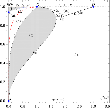
Figure 1: All electrically charged solutions in a $\frac{q^{2}}{R^{2}}\times\frac{r_{0}}{R}$ space. The regions, lines, and points shown in the plot are explained in detail in the text. White regions consist of regular solutions and gray regions consist of singular solutions.

Figure 2: A blow up of the previous figure to show region (e2).

Region (b) contains regular overcharged stars, so $m^{2}<q^{2}$. These are all tension stars for which $\rho(r)>0$ and $p(r)<0$, and that also satisfy the positive enthalpy condition $h(r)=\rho(r)+p(r)>0$. This is a region of interest for the stability problem.

Point $Q$ from the left is extraordinarily interesting. It represents quasiblack holes, which we abbreviate as QBHs from now onward, and these obey $\frac{r_{0}}{R}=1$ and $\frac{q^{2}}{R^{2}}=1$. It is a degenerated point since at $Q$ there exist many solutions with different physical and geometrical properties which depend on the path followed to approach $Q$. The solution may be a pressure quasiblack hole if the point is reached from region (a), a pressureless quasiblack hole if the point is reached by following the line $C_{0}$, a tension quasiblack hole, if the point $Q$ is reached from region (b). We study below in detail these quasiblack hole limits. This is a point of high interest for the stability problem, as a limiting point, indeed, to find the stability character of this point from the left is one of the main motivations of the whole work.

Line $C_{1}$ obeys the equation $a\left(\frac{r_{0}}{R},\frac{q^{2}}{R^{2}}\right)=0$. It contains singular objects. This is a line of no interest for the stability problem.

Region (c) contains singular overcharged objects, so $m^{2}<q^{2}$. These are weird objects having the curvature scalars and the fluid quantities diverging at some radius inside the matter distribution. This is a region of no interest for the stability problem.

Line $C_{2}$ obeys the equation $a\left(\frac{r_{0}}{R},\frac{q^{2}}{R^{2}}\right)=1$. The pressure of all objects on this line is zero, and they are all extremely charged singular black holes with $m^{2}=q^{2}$, i.e., $r_{-}=r_{+}$, and such that $r_{0}<r_{-}=r_{+}$. On this line, the solutions are singular as the energy density and the charge density, which obey $\rho(r)=\rho_{e}(r)$, diverge at $r=0$. This line $C_{2}$ has an elbow at $\frac{q^{2}}{R^{2}}=\frac{27}{16}=1.6875$. Line $C_{0}$ together with line $C_{2}$ form a closed curved in the parameter with equation $a\left(\frac{r_{0}}{R},\frac{q^{2}}{R^{2}}\right)=1$. This is a line of interest for the stability problem as it is a division line to regular black holes.

Line $\dfrac{r_{0}}{R}=\dfrac{r_{-}}{R}=0$ is the horizontal axis. It is a limiting line on which some of the quantities such as the mass diverge. The solutions belonging to this line are not compact objects, they correspond to Kasner spacetimes. This is a line of no special interest for the stability problem.

Point $S$ is the origin of the two axis, it obeys $\frac{q^{2}}{R^{2}}=0$ and $\frac{r_{0}}{R}=0$. It represents different spacetimes depending on the path followed to get there. For instance, it gives the Schwarzschild black hole if the limit is taken by choosing the ratio $\frac{q^{2}}{r_{0}}$ as a fixed finite number. This point is of no special interest for the stability analysis.

Region (d1) contains regular black holes with a central core of charged phantom matter for which $h(r)=\rho(r)+p(r)<0$ up to the boundary radius $r_{0}$ with the radius of the object $r_{0}$ being inside the Cauchy horizon, i.e., $r_{0}<r_{-}=m-\sqrt{m^{2}-q^{2}}$. The energy density $\rho(r)$ is negative for a range of the radial coordinate $r$ inside the matter core, while the pressure $p(r)$ is negative everywhere in the matter region. Regular black holes are always interesting, so despite this negativity of the energy density, they count as interesting solutions. This is a region of interest for the stability problem.

Line $C_{31}$ is drawn from two conditions, the first is that $h(r_{0})=\rho(r_{0})=0$, which in turn implies $\frac{q^{2}}{R^{2}}=\frac{3r_{0}^{4}}{R^{4}}$, and the second is that it verifies that $h(r)$ has finite negative values for all $r$ inside the region of matter distribution. A segment of this line separates region (d1) from region (d2), the other segment of this line separates region (d1) from region (e1). This latter segment coincides with a segment of the line $C_{32}$. This conjoint segment will then be called $C_{31}C_{32}$. This is a line of interest for the stability problem.

Region (d2) contains regular black holes with a central core of charged phantom matter for which the enthalpy $h(r)=\rho(r)+p(r)<0$ close to the center and changes sign toward the surface at radius $r_{0}$, with $r_{0}$ being inside the Cauchy horizon, i.e., $r_{0}<r_{-}=m-\sqrt{m^{2}-q^{2}}$, so that all the matter is fully inside the Cauchy horizon. The energy density is positive and finite at the center, changes to negative values at some $r<r_{0}$ and changes back to positive values close to the surface. This kind of configurations was not separated in LemosZanchin2017 where region (d) is now the region (d1) plus the region (d2). It turns out that the sign change of the enthalpy inside the matter core turns the region (d2) different from region (d1) regarding the stability analysis. This region is a region of interest for the stability problem.

Line $C_{32}$ is drawn by the condition that the solution has $\rho(r)=0$ for some $r$ inside the matter distribution region and $\rho(r)\geq 0$ for all $r$. A segment of this line separates region (d2) from region (e1), the other segment of this line separates region (d1) from region (e1). This is a line of interest for the stability problem.

Region (e1) contains regular black holes with charged phantom matter for which $h(r)=\rho(r)+p(r)>0$ from some radius $r$ up to the boundary radius $r_{0}$ with the radius of the object $r_{0}$ being inside the Cauchy horizon, i.e., $r_{0}<r_{-}=m-\sqrt{m^{2}-q^{2}}$, so that all the matter is fully inside the Cauchy horizon. In this region the energy density is positive, $\rho(r)>0$, for all $0\leq r\leq r_{0}$. Regular black holes are always interesting, and these having positive energy density are certainly interesting solutions. This is a region of interest for the stability problem.

Line $C_{33}$ is drawn by using the condition that the solution has vanishing central enthalpy density, i.e., $h(r=0)=\rho(r=0)+p(r=0)=0$, and it also happens that the configurations on this curve have an enthalpy density $h(r)=\rho(r)+p(r)$ which is positive for all $r$ in the interval $0<r\leq r_{0}$. This line is not explicitly shown in LemosZanchin2017 . Line $C_{33}$ separates region (e1) from region (e2), and is shown in Fig. 2 which is a blow of this zone of Fig. 2. This is a line of interest for the stability problem.

Region (e2) contains regular black holes with a central core of charged matter for which $h(r)=\rho(r)+p(r)>0$ up to the boundary radius $r_{0}$, with $r_{0}$ being inside the Cauchy horizon, i.e., $r_{0}<r_{-}=m-\sqrt{m^{2}-q^{2}}$, so that the all the matter is fully inside the Cauchy horizon. This region has positive energy $\rho(r)>0$ and negative pressure $p(r)<0$. This kind of configurations was not shown in LemosZanchin2017 where region (e) is the region (e1) plus the region (e2). It turns out that regarding the stability analysis the kind of configurations in (e1) needs to be treated separately from objects of region (e2). The region (e2) is shown in Fig. 2 which is a blow of this zone of Fig. 2. This is a region of interest for the stability problem.

Line $\dfrac{r_{0}}{R}=\dfrac{r_{-}}{R}=1$ is the semi-infinite line with $\frac{r_{0}}{R}=1$ and $1<\frac{q^{2}}{R^{2}}<\infty$ in Fig. 2. On this line, the object has a boundary surface $r_{0}$ of the matter that coincides with the de Sitter horizon of the inner metric and with the inner horizon of the Reissner-Nordström exterior metric, the matching being on a lightlike surface. There are two distinguished points on this line, the point $Q$ at $\frac{q^{2}}{R^{2}}=1$, and the point $D$ at $\frac{q^{2}}{R^{2}}=3$, both containing configurations with special properties. The segment of this line in the interval $1<\frac{q^{2}}{R^{2}}<3$ is the top boundary of region (e2), and the $\frac{q^{2}}{R^{2}}>3$ line is part of the top boundary of region (d1). On this line, the metric coefficient $B(r)$ takes the simple form $B(r)=\frac{1}{4}\left(\frac{q^{2}}{R^{2}}-1\right)^{2}\left(1-\frac{r^{2}}{R^{2}}\right)$. After a time reparameterization of the form $\frac{1}{4}\left(\frac{q^{2}}{R^{2}}-1\right)^{2}dt^{2}\to dt^{2}$ the metric potentials turn into a de Sitter metric, i.e., $B(r)=A^{-1}(r)=\left(1-\frac{r^{2}}{R^{2}}\right)$. In the interior region, i.e., for $0\leq\frac{r}{R}<\frac{r_{0}}{R}$, the energy density and pressure for the configurations in this line are given by $8\pi\,\rho(r)=\frac{3}{R^{2}}$ and $8\pi\,p(r)=-\frac{3}{R^{2}}$, so that the equation of state is a de Sitter one, $\rho=-p$, and with the charge density tending to a Dirac delta function centered at the boundary surface $r=r_{0}$. At the boundary $r_{0}$, where here $r_{0}=r_{-}=R$, the energy density jumps from the value $8\pi\,\rho(r)=\frac{3}{R^{2}}$ to the value $8\pi\,\rho(r_{0})=\frac{3}{R^{2}}-\frac{q^{2}}{R^{4}}$, and the pressure jumps from the value $8\pi\,p(r)=-\frac{3}{R^{2}}$ to zero value, $8\pi\,p(r_{0})=0$. Therefore, the enthalpy is zero throughout the matter region, $\rho(r)+p(r)=0$, except at the boundary surface, since there generically the energy density is nonzero, $\rho(r_{0})\neq 0$, and the pressure is zero, $p(r_{0})=0$. There is an exception: at the point $\frac{q^{2}}{R^{2}}=3$, point $D$, the energy density is zero, $\rho(r_{0})=0$, and since the pressure is also zero, the enthalpy is zero, so that the enthalpy is zero throughout the matter region up to and including the boundary $r_{0}$, making point $D$ a special point. This is a line of interest for the stability problem.

Point $D$ is a special and very interesting point. It represents a regular de Sitter black hole with an electric charge coat at the boundary. This boundary is a lightlike surface at $r_{0}=r_{-}$. The interior solution is pure de Sitter. For $0\leq\frac{r}{R}<\frac{r_{0}}{R}$, the energy density is given by $8\pi\,\rho(r)=\frac{3}{R^{2}}$ and the pressure by $8\pi\,p(r)=-\frac{3}{R^{2}}$, so that $\rho+p=0$, i.e., a cosmological constant equation of state is verified in this region. For $\frac{r}{R}=\frac{r_{0}}{R}$, i.e., $r=r_{0}$, the energy density is given by $8\pi\,\rho(r_{0})=0$ and the pressure by $8\pi\,p(r)=0$, so that obviously $\rho+p=0$ in this surface, a feature that does not happen for the other black holes on the line $r_{0}=r_{-}=R$. Thus, from the interior up to the boundary itself, the enthalpy is zero, $\rho+p=0$. This solution is one of the regular black holes found in LemosZanchin2011 . Point $D$ has physical interest in itself and surely is of interest for the stability problem.

Point $Q$ from the right is also extraordinarily interesting. It represents quasinonblack holes, which we abbreviate as QNBHs from now onward. It is degenerated since there exist many solutions with different physical and geometrical properties for the same parameters, $\frac{r_{0}}{R}=1$ and $\frac{q^{2}}{R^{2}}=1$, depending on the path followed from the right to approach that point. The solutions have different characteristics depending if point $Q$ is reached from regions (d2), (e1), or (e2). All these differences will be reflected in the stability analysis. We study in detail below the QNBH limits. Point $Q$ from the right is a point of high interest for the stability problem, as a limiting point.

Line $\dfrac{r_{0}}{R}=\dfrac{r_{+}}{R}=1$ is the segment of the line $\frac{r_{0}}{R}=1$ with the electric charge in the interval $0<\frac{q^{2}}{R^{2}}<1$. It contains singular objects. This is a line of no special interest for the stability problem.

Region (f) contains singular undercharged solutions, so $m^{2}>q^{2}$. These are all objects for which the energy density and the pressure diverge at some $r$ inside the matter distribution. This is a region of no interest for the stability problem.

Line $C_{4}$ is the Buchdahl-Andréasson bound line characterized by the central pressure of any object lying on this line being infinite. One of the endpoints of this line is point $B$, the Buchdahl bound point. This is a line of interest for the stability problem, as a limiting line.

The description ends here, as the next line would be the vertical axis that we have already described.

III.3 The quasiblack hole and quasinonblack hole limits

III.3.1 The five distinct quasiblack holes and quasinonblack holes

As pointed out in LemosZanchin2010 , the solutions we are treating admit QBHs. This happens when the mass $m$ approaches the electric charge $q$, $m^{2}\rightarrow q^{2}$, and the boundary radius $r_{0}$ approaches the gravitational radius $r_{+}$, $r_{0}\to r_{+}$, or equivalently $\frac{q^{2}}{R^{2}}\to 1$ and $\frac{r_{0}}{R}\to 1$, so that one reaches the point $Q$ of Fig. 2. As also pointed out in LemosZanchin2017 , the point $Q$ is a degenerate point which represents several different kinds of objects. However, one has to distinguish when $Q$ is approached from the left, which can give rise to QBHs, from when $Q$ is approached from the right, which can give rise to QNBHS. QNBHs have their own properties distinct from the properties of QBHs, as found in lemosluz2021 .

QBHs are obtained by compressing star-like configurations with radius $r_{0}$ quasistatically to the gravitational radius $r_{+}$, $r_{0}\to r_{+}$. In this limiting process one arrives at point $Q$ from the left, i.e., from the region of the parameter space for which $\frac{q^{2}}{R^{2}}<1$, and also leads to $r_{0}\to r_{+}\to r_{-}$. The result is a starlike configuration on the verge of being an extremely charged Reissner-Nordström black hole, but instead becoming an extremely charged Reissner-Nordström QBH.

QNBHs are obtained by decompressing regular black hole configurations for which the radius $r_{0}$ is smaller than the inner radius $r_{-}$, $r_{0}<r_{-}$, up to the radius $r_{-}$, $r_{0}\to r_{-}$. In this limiting process one arrives at point $Q$ from the right, i.e., from the region of the parameter space for which $\frac{q^{2}}{R^{2}}>1$, and leads to $r_{0}\to r_{-}\to r_{+}$. The result is a regular black hole on the verge of not being an extremely charged regular Reissner-Nordström black hole, but instead becoming an extremely charged Reissner-Nordström QNBH.

From the analysis of the liming procedure on the several different classes of regular objects just performed, one finds conclusively that QBH and QNBH configurations may be obtained. This can also be confirmed by direct inspection of Fig. 2. We now enumerate and describe the five types that are obtained in the limiting procedure, with three types being QBHs and two types being QNBHs.

(i) QBHs from regular undercharged pressure stars: These arise from region (a), with the parameter $a$ in the range $1<a<8$ approximately, below the line $C_{4}$ and above the line $C_{0}$ in Fig. 2. These QBHs form from distributions of charged matter for which the electric repulsion is less than the gravitational attraction and there is matter pressure, $p>0$. The resulting objects are pressure QBHs, with $m^{2}=q^{2}$. They are nonsingular, no curvature invariant diverges for the whole spacetime. In the figure this case corresponds to taking the limit to the point $Q$ from region (a), which means $a>1$ and $\frac{q^{2}}{R^{2}}<\frac{r_{0}^{4}}{R^{4}}\leq 1$ with the equality holding just at $Q$. These configurations satisfy all the energy conditions and the causality condition as long as $1<a<\frac{4}{3}$. This type of QBHs has been investigated in detail in LemosZanchin2010 .

(ii) QBHs from extremal charged dust stars: These arise from line $C_{0}$ in Fig. 2, have $a=1$, which means $\frac{q^{2}}{R^{2}}=\frac{r_{0}^{2}}{R^{2}}\left(2-\frac{r_{0}^{2}}{R^{2}}-2\sqrt{1-\frac{r_{0}^{2}}{R^{2}}}\right)$. These configurations follow from distributions of extremal charged dust, for which the electric repulsion counterpoises the gravitational attraction and there is no matter pressure, $p=0$. The resulting objects are extremal QBHs, with with $m^{2}=q^{2}$. They are nonsingular, no curvature invariant diverges for the whole spacetime. In the figure, this case corresponds to taking the limit to the point $Q$ along the curve $C_{0}$. This type of QBHs has been investigated in LemosWeinberg2004 , see also lemoszanchin2008 .

(iii) QBHs from overcharged tension stars: These arise from region (b), with $0<a<1$ and $\frac{q^{2}}{R^{2}}<\frac{r_{0}^{4}}{R^{4}}$, between lines $C_{0}$ and $C_{1}$ in Fig. 2. These configurations follow from distributions of charged matter, for which the electric repulsion is greater than the gravitational attraction and there is matter tension, $p<0$. The resulting objects are tension QBHs, with $m^{2}=q^{2}$. They are nonsingular, no curvature invariant diverges for the whole spacetime. This type of QBHs has been investigated in LemosZanchin2010 .

(iv) QNBHs from regular phantom black holes: These arise from regions (d2) and (e1), with $1<a<4$, and $\frac{q^{2}}{R^{2}}\geq 1$, in Fig. 2. These configurations follow from regular electrically charged black holes, for which the matter is phantom, i.e., $\rho+p<0$ everywhere. The resulting objects are regular phantom QNBHs, with $m^{2}=q^{2}$. In the figure this case corresponds to taking the limit to the point $Q$ from regions (d2) and (e1). This type of QNBHs has not been investigated, see lemosluz2021 for an example of QNBHs.

(v) QNBHs from regular normal black holes: These arise from region (e2), with $a>4$ approximately in Fig. 2 which is a zoom of Fig. 2 to see this region. These configurations follow from regular electrically charged regular black holes, for which the matter is normal, i.e., $\rho+p>0$ everywhere, with the pressure being negative. The resulting objects are regular tension QNBHs, with $m^{2}=q^{2}$. In the Fig. 2 this case corresponds to taking the limit to the point $Q$ from region (e2). This type of QNBHs has not been investigated, see lemosluz2021 for an example of QNBHs.

III.3.2 Taking the limits to obtains quasiblack holes and quasinonblack holes

The Guilfoyle parameter $a$, which by Eq. (55) is a function of $\frac{q^{2}}{R^{2}}$ and $\frac{r_{0}}{R}$ by Eq. (55), is not well defined in the limit to the point $Q$. In fact, the parameter $a$ may assume any value there, depending on the path followed in the parameter space to reach that point. To see this we write $\frac{q^{2}}{R^{2}}=\left(1\pm 2\sqrt{\varepsilon}\right)\frac{r_{0}^{4}}{R^{4}}$ and $\frac{r_{0}^{2}}{R^{2}}=1-\delta$, where $\varepsilon$ and $\delta$ are small nonnegative parameters. Upon substituting these expansions into Eq. (55) one gets $a=\frac{\varepsilon}{\delta}$ up to the correct order. Thus, clearly, in the limits $\varepsilon\to 0$ and $\delta\to 0$ the parameter $a(\frac{q^{2}}{R^{2}},\frac{r_{0}}{R})$ is not a well defined function. It follows that, by parameterizing the problem in terms of $\frac{q^{2}}{R^{2}}$ and $\frac{r_{0}}{R}$, it is difficult to keep control of the values of $a$ during numerical calculations when approaching the point $Q$. This control is necessary to analyze the stability conditions of the QBH and QNBH limits within each region of Fig. 2 near the point $Q$.

In order to avoid such a lack of control, we should choose a particular relation between $\varepsilon$ and $\delta$, $\varepsilon=\varepsilon(\delta)$, and in doing so a specific path has been chosen in the parameter space. This is equivalent to choose a specific relation between the two independent parameters $\frac{q^{2}}{R^{2}}$ and $\frac{r_{0}}{R}$ and letting $a$ as a free parameter, as it was done in LemosZanchin2010 . To follow this rationale, we need to write $\frac{q^{2}}{R^{2}}$ as a function of $a$ and $\frac{r_{0}}{R}$, which can be done by means of Eq. (55). To proceed, we write

$$\frac{r_{0}^{2}}{R^{2}}=1-\delta,$$ (56)

with $\delta$ being a small positive number and with Eq. (56) being valid in first order in $\delta$, i.e., in a region close to the point $Q$. With this assumption, the leading terms in the expression for $\frac{q^{2}}{R^{2}}$ obtained from Eq. (55) may be written as $\frac{q^{2}}{R^{2}}=1\pm 2\sqrt{a\,\delta}+2\left(a-1\right)\delta$, or equivalently $\frac{q^{2}}{R^{2}}=\left[1\pm 2\sqrt{a\,\delta}+\left(2a-1\right)\delta\right]\frac{r_{0}^{2}}{R^{2}}$. Since $\delta$ is small and arbitrary, for finite $a$ we may write $a\,\delta\equiv\varepsilon$, i.e., Eq. (55) together with Eq. (56) leads to

$$\frac{q^{2}}{R^{2}}=\left[1\pm 2\sqrt{\varepsilon}+\left(2a-1\right)\frac{\varepsilon}{a}\right]\frac{r_{0}^{2}}{R^{2}},$$ (57)

where $\varepsilon$ is a small nonnegative parameter given in terms of $a$ and $\delta$ by

$$\varepsilon=a\delta.$$ (58)

This relation means that the point $Q$ is approached by following straight lines in the parameter space, with the $\pm$ signs indicating if one reaches that point from the right side or from the left side. Since each constant $a$ defines a curve in the parameter space, and all the curves for different values of $a$ reach the point $Q$, the parameter $a$ is the appropriate parameter to be used as a free parameter for the present analysis. Hence, from now on we choose as free parameters $a$ and $\frac{r_{0}}{R}$, instead of $\frac{q^{2}}{R^{2}}$ and $\frac{r_{0}}{R}$, with intervals $0<a<\infty$ and $0\leq\frac{r_{0}}{R}\leq 1$. Moreover, on one hand, the minus sign in Eq. (57) indicates paths approaching the point $Q$ from the left, i.e, with $\frac{q^{2}}{R^{2}}<1$, which contains star configurations in regions (a) and (b), and other singular objects in regions (c) and (f). In this case, the limits $\varepsilon\to 0$ and $\delta\to 0$ take the radius of the object under consideration, be it a star or a singular configuration, to the limit of the gravitational radius, i.e., almost to a black hole which is the QBH limit LemosWeinberg2004 . On the other hand, the plus sign in Eq. (57) indicates paths approaching the point $Q$ from the right, i.e., with $\frac{q^{2}}{R^{2}}>1$, which corresponds to other singular objects in the region (c), and black hole configurations in the regions (d2), (e1), and (e2). In this case, the limits $\varepsilon\to 0$ and $\delta\to 0$ take the boundary matter in region (c) to the limit of the gravitational radius, i.e., almost to a black hole which is the QBH limit [6], and take the boundary matter in the regions (d2), (e1), and (e2) to the Cauchy horizon radius which is equal to the event horizon radius, i.e., to the QNBH limit lemosluz2021 . Then, we rewrite the relevant equations of the model in terms of $a$ and $\frac{r_{0}}{R}$ up to first order in $\varepsilon$ and, at the end, take the limit $\frac{r_{0}}{R}\to 1-\frac{\delta}{2}$, with $\delta$ related to $\varepsilon$ through Eq. (58). For instance, one finds that, at the lowest orders in $\varepsilon$, Eq. (54) implies in $\frac{m}{r_{0}}=1\pm\sqrt{\varepsilon}+\left(a-1\right)\frac{\varepsilon}{a}$ which, together with Eq. (57), gives $\frac{m^{2}}{q^{2}}=1+\frac{a-1}{a}\varepsilon$. Notice then that one gets $\frac{m^{2}}{q^{2}}<1$ for $0<a<1$ as expected, and $\frac{m^{2}}{q^{2}}\geq 1$ for $a\geq 1$ as also expected. Using the same procedure one also finds that the constants $k_{0}$ and $k_{1}$ that appear in the expressions for the metric functions, matter functions, and electric functions are $k_{0}=\mp a^{\frac{1}{a}}\varepsilon^{\frac{a-2}{2a}}$, and $k_{1}=\pm\frac{\sqrt{a}\,k_{0}}{2-a}=-\frac{a^{\frac{a+2}{2a}}}{2-a}\varepsilon^{\frac{a-2}{2a}}$. All equalities are approximate equalities, correct up to the first order in the expansion.

We now find the expressions for the metric potentials, the matter functions, the electric potential, and the electric charge, when the configurations approach the QBH or the QNBH limits. Taking the expansions given in Eqs. (56)-(58) and the approximations for $k_{0}$ and $k_{1}$ presented in the last paragraph into the corresponding equations for the metric potentials, Eqs. (45)-(46), we find

$$A(r)=\left(1-\dfrac{r^{2}}{r_{0}^{2}}\left[1-\dfrac{\varepsilon}{a}\right]\right)^{-1},$$ (59)

$$B(r)=\left(1\mp\dfrac{2-a}{\sqrt{a\,}}\sqrt{1-\dfrac{r^{2}}{r_{0}^{2}}}\right)^{\!\!\frac{2a}{a-2}}\!\!\!\dfrac{\varepsilon}{a}\,,$$ (60)

where we have written $R$, $m$, and $q$ in terms of $a$, $r_{0}$, and $\varepsilon$. All equalities are valid up to first order. Now, taking the expansions given in Eqs. (56)-(58) into the corresponding equations for the fluid quantities, namely, the energy density and the pressure, Eqs. (47)-(48), one finds

$$\!\!\!8\pi\rho(r) = \dfrac{3}{r_{0}^{2}}-\dfrac{r^{2}}{r_{0}^{4}\,}\left(\frac{2-a}{\sqrt{a\,}}\,\sqrt{1-\dfrac{r^{2}}{r_{0}^{2}}}\mp 1\right)^{\hskip-4.26773pt-2},$$ (61)

$$8\pi p(r) \!=\! -\frac{1}{r_{0}^{2}}+\frac{r^{2}}{r_{0}^{4}\,}\left(\frac{2-a}{\sqrt{a\,}}\,\sqrt{1-\dfrac{r^{2}}{r_{0}^{2}}}\mp 1\right)^{\hskip-4.26773pt-2}$$ (62)

$$+\dfrac{2\,\sqrt{a\,}}{r_{0}^{2}}\sqrt{1-\dfrac{r^{2}}{r_{0}^{2}}}\,\left(\frac{2-a}{\sqrt{a}}\sqrt{1-\dfrac{r^{2}}{r_{0}^{2}}}\mp 1\right)^{\hskip-4.26773pt-1}.$$

These are the zeroth order approximations for $\rho(r)$ and $p(r)$ in which $\frac{r_{0}^{2}}{R^{2}}=1$ and, as a consequence, $m^{2}=q^{2}=r_{0}^{2}$.

Taking the expansions into the corresponding equation for the electric potential of the interior region, Eq. (49), one finds

$$\phi(r)=\epsilon\left(1\mp\dfrac{2-a}{\sqrt{a\,}}\sqrt{1-\dfrac{r^{2}}{r_{0}^{2}}}\right)^{\!\!\frac{a}{a-2}}\!\!\!\dfrac{\sqrt{\varepsilon}}{a}\,.$$ (63)

Taking the expansions given in Eqs. (56)-(58) into the corresponding equation for the electric charge of the interior region, Eq. (50), one finds

$$Q(r)=\dfrac{\epsilon r^{3}}{r_{0}^{2}}\left(\frac{2-a}{\sqrt{a\,}}\,\sqrt{1-\dfrac{r^{2}}{r_{0}^{2}}}\mp 1\right)^{\hskip-4.26773pt-1}.$$ (64)

that is also a zeroth order approximation such that $r_{0}=R$,

Similarly, the approximated expressions of all quantities related to the exterior solution are obtained. The corresponding limits for the metric potentials of the exterior region solution, with $r\geq r_{0}$, can be obtained. The potential $A(r)$ in Eq. (51) is then

$$\hskip-5.69046ptA(r)\hskip-4.26773pt=\hskip-4.26773pt\left[\left(1\hskip-1.42271pt-\hskip-1.42271pt\dfrac{r_{0}}{r}\left[1\pm\sqrt{\varepsilon}\right]\right)^{\!\!2}\hskip-1.42271pt-\hskip-1.42271pt\dfrac{r_{0}}{r}\left(2\hskip-1.42271pt-\hskip-1.42271pt\dfrac{r_{0}}{r}\right)\dfrac{a-1}{a}\varepsilon\right]^{-1}\hskip-8.5359pt,$$ (65)

and the potential $B(r)=\dfrac{1}{A(r)}$ in Eq. (52) is then

$$\hskip-8.5359ptB(r)=\left(1-\dfrac{r_{0}}{r}\left[1\pm\sqrt{\varepsilon}\right]\right)^{\!\!2}-\dfrac{r_{0}}{r}\left(2-\dfrac{r_{0}}{r}\right)\dfrac{a-1}{a}\varepsilon.$$ (66)

Taking the expansions into the corresponding equation for the electric potential of the exterior region, Eq. (53), one finds

$$\phi(r)=\epsilon\left(\dfrac{r_{0}}{r}-1\right)\left(1\pm\sqrt{\varepsilon}\right)+\epsilon\dfrac{\sqrt{\varepsilon}}{a},$$ (67)

where the integration constant has been adjusted so that the function in (67) equals the function for the interior electric potential given in (63) at the boundary.

The approximate relations given in this section hold for both QBH and QNBH cases, with the lower sign in $\pm$ or $\mp$ holding for QBH configurations while the upper sign holds for QNBH configurations. QBHs occur for $a>1$ with $\frac{q^{2}}{R^{2}}=1-2\sqrt{\varepsilon}$ and for $0<a\leq 1$ with $\frac{q^{2}}{R^{2}}=1-2\sqrt{\varepsilon\,}$. QNBHs occur for $a>1$ with $\frac{q^{2}}{R^{2}}=1+2\sqrt{\varepsilon\,}$. The relations given in Eqs. (61), (62), and (64) are the zeroth order approximations in $\sqrt{\varepsilon\,}$. The other relations are first order approximations in $\sqrt{\varepsilon\,}$.

III.4 Summary of the plethora of solutions

Within the electrically charged spherically symmetric solutions presented here, there are many solutions of interest, either because they may represent actual objects within the physical universe, or they have in themselves interesting physical features, like a rich causal behavior, relevant matter characteristics, or some other important aspect. Almost all these solutions have a core of electrically charged matter and a Reissner-Nordström exterior, excluding some degenerate cases that we have mentioned.

A sketch of all solutions that naturally appeared within the class studied is given in Table 1. A concise description of these solutions is now given. With respect to objects that can be classified as stars, i.e., star solutions, there is a list that we should refer to. There are the interior Schwarzschild solutions, i.e., Schwarzschild stars, the first member of this family being a black hole, and the last member of the family being the Schwarzschild star saturating the Buchdahl bound. There are also uncharged singular star solutions. There are undercharged stars, the last members of this family are stars saturating the Buchdahl-Andréasson bound. There are also undercharged singular star solutions. There are extremally charged objects, i.e., the Bonnor stars, the exterior being an extremely Reissner-Nordström spacetime. There are tension overcharged stars. There are QBHs that appear in distinct forms, namely, pressure QBHs, pressureles QBHs, and tension QBHs. There are also singular overcharged objects and singular extremely charged objects. There are Kasner like objects, which are highly singular. With respect to objects that can be classified as regular black holes there is the following list. There are regular black holes with negative energy densities, regular black holes with a central core of charged phantom matter, regular tension black holes with positive enthalpy density, and there is a regular de Sitter black hole with an electric charge coat at the boundary. There are QNBHs. There is also a number of nonregular black holes. All these different solutions are found within the class of the Guilfoyle solution presented above.

The stability of an object and of a solution is an important feature that it must possess in order to be considered of relevance in the set of natural objects. Thus, we now turn to the stability problem of these objects.

Configurations	Features	Location in the parameter space
Schwarzschild stars	uncharged, regular	Line $\frac{q^{2}}{R^{2}}=0$, $0<\frac{r_{0}}{R}<\frac{2\sqrt{2}}{3}$
Buchdahl limit	singular Schwarzschild star	Point $B$: $\frac{q^{2}}{R^{2}}=0$, $\frac{r_{0}}{R}=\frac{2\sqrt{2}}{3}$
Undercharged stars	regular, $q^{2}<m^{2}$	Region ($a$)
Buchdahl-Andréasson limit	singular undercharged star	Line $C_{4}$
Undercharged stars	singular, $q^{2}<m^{2}$	Region ($f$)
Extremely charged stars	regular, $q^{2}=m^{2}$	Line $C_{0}$
Overcharged tension stars	regular, $q^{2}>m^{2}$, $-1<\frac{p}{\rho}<0$	Region ($b$)
Overcharged tension stars	singular, $q^{2}>m^{2}$	Line $C_{1}$ and region ($c$)
Extremely charged stars	singular, $q^{2}=m^{2}$	Line $C_{2}$
Regular phantom black holes	$q^{2}<m^{2}$, phantom matter: $\frac{p}{\rho}<-1$	Regions ($d_{1}$) and ($d_{2}$), and line $C_{31}$
Regular phantom black holes	$q^{2}<m^{2}$, phantom matter: $-1<\frac{p}{\rho}<0$, $\rho<0$	Region ($e_{1}$) and line $C_{32}$
Regular tension black holes	$q^{2}<m^{2}$, $-1<\frac{p}{\rho}<0$, $\rho>0$	Region ($e_{2}$)
Regular de Sitter black hole	$q^{2}<m^{2}$, $\frac{p}{\rho}=-1$, $\rho>0$	Point $D$: $\frac{q^{2}}{R^{2}}=3$, $\frac{r_{0}}{R}=1$
Regular pressure quasiblack holes	$q^{2}=m^{2}$, regular pressure core: $\frac{p}{\rho}>0$	Point Q from region ($a$)
Singular quasiblack holes	$q^{2}=m^{2}$, singular pressure core: $\frac{p}{\rho}>0$	Point Q from region ($f$) and line $C_{4}$
Regular quasiblack holes	$q^{2}=m^{2}$, regular pressureless core: $\frac{p}{\rho}=0$	Point Q from line $C_{0}$
Regular tension quasiblack holes	$q^{2}=m^{2}$, regular tension core: $-1<\frac{p}{\rho}<0$	Point Q from region ($b$)
Singular quasiblack holes	$q^{2}=m^{2}$, singular tension core: $-1<\frac{p}{\rho}<0$	Point Q from line $C_{1}$ and region ($c$)
Singular quasiblack holes	$q^{2}=m^{2}$, singular pressureless core: $\frac{p}{\rho}=0$	Point Q from line $C_{2}$
Regular quasinonblack holes	$q^{2}=m^{2}$, phantom matter: $\frac{p}{\rho}<-1$	Point Q from region ($d_{2}$)
Regular quasinonblack holes	$q^{2}<m^{2}$, phantom matter: $-1<\frac{p}{\rho}<0$, $\rho<0$	Point Q from region ($e_{1}$) and line $C_{32}$
Regular tension quasinonblack holes	$q^{2}<m^{2}$, $-1<\frac{p}{\rho}<0$, $\rho>0$	Point Q from region ($e_{2}$)
Kasner spacetimes		Line $\frac{r_{0}}{R}=0$, $\frac{q^{2}}{R^{2}}>0$

Table 1: The plethora of solutions.

IV Stability analysis of the electric charged spheres: Results for regular stars, regular black holes, quasiblack holes, and quasinonblack holes

IV.1 The stability of regular stars

IV.1.1 Zero electric charged stars: $\frac{q^{2}}{R^{2}}=0$, i.e., Schwarzschild stars

The Schwarzschild star solutions, composed of a Schwarzschild interior and a Schwarzschild exterior vacuum solution, are given by $\frac{q^{2}}{R^{2}}=0$ with variable $\frac{r_{0}}{R}$. The expressions for the metric potentials, the fluid quantities, and the electric quantities, are obtainable from Guilfoyle’s solution, see LemosZanchin2017 . In Fig. 2 these Schwarzschild stars correspond to the vertical axis.

In this case, the energy density and the pressure are positive functions everywhere inside the matter. Thus, one finds that the enthalpy $h(r)=\rho(r)+p(r)>0$ and, as a consequence, assuming that the adiabatic index obeys $\gamma>0$, the coefficients $F(r)$ and $W(r)$ that appear in Eq. (35) are both positive functions, and so in the SL problem this leads to the case (A) of the theorem given in Appendix C. Therefore, stable solutions to radial perturbations are found for positive adiabatic indices such that $\gamma>\gamma_{\rm cr}$, where $\gamma_{\rm cr}$ is the critical value, the minimum value of $\gamma$ for which the solution is stable, see Chandre1964b . We note here, in passing, that for numerical analysis the frequency $\omega$ is normalized as $\omega R$. From this section onward, including all the figures dealing with stability, we drop $R$ to simplify notation.

In Fig. 3 we show the numerical results for the critical adiabatic index $\gamma_{\rm cr}$ as a function of the normalized radius of the star $\frac{r_{0}}{R}$ for zero electric charge, $\frac{q^{2}}{R^{2}}=0$. The vertical axis bounds the plot on the left. The vertical dotted line on the right in the plot is the Buchdahl bound AndreassonQ , see also LemosZanchin2015 , which is represented by point $B$ in Fig. 2. In the plot there is the white region that represents the range of the parameter $\frac{r_{0}}{R}$ where regular

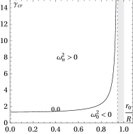
Figure 3: Stability of zero charge stars, i.e., Schwarzschild stars. These stars are on the vertical line $\frac{q^{2}}{R^{2}}=0$ of Fig. 2. The critical adiabatic index $\gamma_{\rm cr}$, which gives the $\gamma$ for which $\omega_{0}^{2}=0$, is shown as a function of the radius $\frac{r_{0}}{R}$. The region above the line is stable to radial perturbations, the region below the line is unstable. It is seen that $\gamma_{\rm cr}$ starts at $\frac{4}{3}$, and as the star gets more compact the $\gamma_{\rm cr}$ gets higher and higher. The light gray region corresponds to stars that are not regular and are beyond the Buchdahl limit.

Schwarzschild stars are found, and the light gray region that contains Schwarzschild stars that are singular. The solid line drawn is for the vanishing fundamental oscillation frequency squared, i.e., for $\omega_{0}^{2}=0$, which means that $\omega_{0}^{2}$ changes sign across this curve. All configurations represented by points located above the $\omega_{0}^{2}=0$ line are stable stars, i.e., all $\omega_{n}^{2}$ are positive, all configurations represented by points located below the $\omega_{0}^{2}=0$ line are unstable stars. The solid line starts at $\frac{r_{0}}{R}=0$ and extends to point $B$, the Buchdahl limit, given by $\frac{r_{0}}{R}=\frac{2\sqrt{2}}{3}=0.943$, where this last equality is approximate, and where $\gamma_{\rm cr}$ diverges. Let us comment in more detail on these configurations and their stability. The limit $\frac{r_{0}}{R}=0$ for zero charge stars means that there is no star. Indeed, for $R$ fixed, taking the limit of $r_{0}$ going to zero means that the mass of the stars goes to zero sufficiently fast so that in the $r_{0}=0$ limit there is no mass and so no star. But since $R$ is fixed, and so the effective density is fixed, although there is no mass, no star, and no gravity, there is a fluid, and this means that the spacetime is that of a fluid composed of test fluid elements in Minkowski spacetime. In this case to be stable the lowest $\gamma_{\rm cr}$ is the $\gamma_{\rm cr}$ for a fluid in the laboratory, with no gravity, and it is $\gamma_{\rm cr}=\frac{4}{3}=1.33$, where this last equality is approximate. It is worth noting that such an interpretation can be given only after the stability analysis is made, because only then it is possible to understand that in this limit there is a test fluid in a Minkowski spacetime rather than pure empty Minkowski spacetime. At the other end of the plot, at the point $B$ in Fig. 2, i.e., for $\frac{r_{0}}{R}=\frac{2\sqrt{2}}{3}=0.943$, where this latter value is an approximate value, it can be taken to mean that for some $R$ fixed, and since $R$ is the inverse of the effective density, for some fixed effective density, there is a sufficiently high $r_{0}$ that makes the star relatively large but compact. It is is indeed a Schwarzschild star at the Buchdahl limit. In this case to be stable a very high $\gamma_{\rm cr}$ is necessary, in the limit $\gamma_{\rm cr}$ has to be infinite to provide a stable star against radial perturbations. Since in this picture we are fixing $R$ and so the effective density of the star, it is the way of considering a compact star as Michell and Laplace have done, namely, the density of the star is given and fixed, the star has relatively large mass and large radius, but is in all measures compact.

In Fig. 4 we show the numerical results for the critical adiabatic index $\gamma_{\rm cr}$ as a function of the normalized radius $\frac{r_{0}}{r_{+}}$ for zero electric charge, namely, $\frac{q^{2}}{R^{2}}=0$. It is interesting to show this new plot of $\gamma_{\rm cr}$ as a function of $\frac{r_{0}}{r_{+}}$ as some features are highlighted and complementary to the plot of Fig. 3, noting that $\frac{r_{0}}{r_{+}}$ and $\frac{r_{0}}{R}$ are convertible from one to the other.

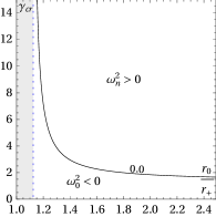
Figure 4: Stability of zero charge stars, i.e., Schwarzschild stars. These stars are on the vertical line $\frac{q^{2}}{R^{2}}=0$ of Fig. 2. The critical adiabatic index $\gamma_{\rm cr}$, which gives the $\gamma$ for which $\omega_{0}^{2}=0$, is shown as a function of the radius $\frac{r_{0}}{r_{+}}$. The region above the line is stable against radial perturbations, the region below the line is unstable. It is seen that for a Schwarzschild star at the Buchdahl limit $\gamma_{\rm cr}$ is unlimited and then decreases up to $\frac{4}{3}$. The light gray region corresponds to stars that are not regular and are beyond the Buchdahl limit.

The vertical dotted line on the left in the plot is the Buchdahl bound AndreassonQ , see also LemosZanchin2015 , which is represented by point $B$ in Fig. 2. On the right the plot extends to infinity. In the plot there is the light gray region that contains singular Schwarzschild stars, and the white region that represents the range of parameter $\frac{r_{0}}{r_{+}}$ where regular Schwarzschild stars are found. The solid line drawn is for the vanishing fundamental oscillation frequency squared, i.e., for $\omega_{0}^{2}=0$, which means that $\omega_{0}^{2}$ changes sign across such a curve. All configurations represented by points located above the $\omega_{0}^{2}=0$ line are stable stars, i.e., all $\omega_{n}^{2}$ are positive, all configurations represented by points located below the $\omega_{0}^{2}=0$ line are unstable stars. The solid line starts at $\frac{r_{0}}{r_{+}}=\frac{9}{8}$ that corresponds to Buchdahl bound, and extends to $\frac{r_{0}}{r_{+}}$ infinitely large. Let us comment in more detail on these configurations and their stability. The limit $\frac{r_{0}}{r_{+}}=\frac{9}{8}$ means that the radius of the star is very compact, indeed it is a Schwarzschild star at the Buchdahl limit, almost at the $r_{0}=r_{+}$ QBH limit. In this case to be stable a very high $\gamma_{\rm cr}$ is necessary, in the limit $\gamma_{\rm cr}$ has to be infinite to provide a stable star against radial perturbations. Since in this picture we are fixing $r_{+}$, and so the spacetime mass, it is the way of considering a compact star as it is nowadays usually done, as for instance in the work of Chandrasekhar Chandre1964b . With the parameter $\frac{r_{0}}{r_{+}}$ one gets the compactness of the star immediately. At the other end, for $\frac{r_{0}}{r_{+}}$ indefinitely large, one has that the radius of the star is very large compared with $r_{+}$ and so the star is extremely disperse. In the limit that $r_{0}$ is infinite there is a fluid made of test fluid elements in a Minkowski background. In this case to be stable the lowest $\gamma_{\rm cr}$ is the $\gamma_{\rm cr}$ for a fluid in the laboratory, with no gravity, and it is $\gamma_{\rm cr}=\frac{4}{3}=1.33$, where this last equality is approximate. Again, this interpretation can be given only after the stability analysis is made, because only then it is possible to understand that in this limit there is a test fluid in a Minkowski spacetime rather than pure empty Minkowski spacetime.

In Table 2 we give details of the numerical results for the stability of the Schwarzschild stars, i.e., zero charged stars. The behavior of $\gamma_{\rm cr}$ as a function of the radius $\frac{r_{0}}{R}$ and $\frac{r_{0}}{r_{+}}$, for $\frac{q^{2}}{R^{2}}=0$, is displayed.

$\frac{r_{0}}{R}$	$\frac{r_{0}}{r_{+}}$	$\gamma_{\rm cr}$	$\gamma_{\rm ch}(1)$ Chandre1964b	$\gamma_{\rm pc}$ PosadaChirenti2019
0.342	8.549	1.39406	1.3940	1.394010
0.500	4.000	1.48957	1.4890	1.489546
0.707	2.000	1.84347	1.8375	1.843456
0.819	1.490	2.55434	2.5204	2.554324
0.907	1.217	6.12566	5.5802	6.125634

Table 2: The critical adiabatic index $\gamma_{\rm cr}$ for the radial perturbations of zero charged stars, $\frac{q^{2}}{R^{2}}=0$, i.e., Schwarzschild stars, with different radii $\frac{r_{0}}{R}$ and $\frac{r_{0}}{r_{+}}$. For not so large $\frac{r_{0}}{R}$, our results are in good agreement with the values $\gamma_{\rm ch}$ found by Chandrasekhar Chandre1964b for various values of the parameter $0.00<\frac{r_{0}}{R}<0.819$, and for all $\frac{r_{0}}{R}$ our results are in good agreement with the values $\gamma_{\rm pc}$ found in PosadaChirenti2019 . These zero charged stars are in the vertical axis $\frac{q^{2}}{R^{2}}=0$ of Fig. 2.

The values of the critical adiabatic index $\gamma_{\rm cr}$ are obtained from the shooting and the pseudospectral methods, and are in agreement to each other up to six decimal places. Our results are in good agreement with the values of the critical adiabatic index $\gamma_{\rm ch}$ calculated in Chandre1964b , see the fourth column of the table, and are in very good agreement with the values of the critical adiabatic index $\gamma_{\rm pc}$ calculated in PosadaChirenti2019 , see the fifth column of the table. Note, however, that there is a difference between the critical $\gamma_{\rm ch}$ calculated by Chandrasekhar Chandre1964b and the critical $\gamma_{\rm pc}$ calculated in PosadaChirenti2019 and by us as $\frac{r_{0}}{R}$ approaches from below $\frac{r_{0}}{R}=\frac{2\sqrt{2}}{3}=0.943$, with the latter number being approximate, and as $\frac{r_{0}}{r_{+}}$ approaches from above $\frac{r_{0}}{r_{+}}=\frac{9}{8}=1.125$, i.e., the Buchdahl point $B$ in Fig. 2. This difference may be explained by the fact that the trial functions used by Chandrasekhar do not approximate the true eigenfunctions in the limit of large $\frac{r_{0}}{R}$ PosadaChirenti2019 .

IV.1.2 Undercharged pressure stars: $0<q^{2}<m^{2}$

Undercharged pressure stars are stars with $0<q^{2}<m^{2}$ and also obey $0<\frac{q^{2}}{R^{2}}<1$. These configurations belong to region (a) between lines $C_{0}$ and $C_{4}$ in Fig. 2.

In this case, the energy density and the pressure are positive functions everywhere inside the matter. Thus, one finds $h(r)=\rho(r)+p(r)>0$ and, as a consequence, assuming $\gamma>0$ the coefficients $F(r)$ and $W(r)$ that appear in Eq. (35) are both positive functions, and so in the SL problem this leads to the case (A) of the theorem given in Appendix C. Therefore, similarly to the case of the zero charged Schwarzschild stars, stable solutions to radial perturbations are found for positive adiabatic indices such that $\gamma>\gamma_{\rm cr}$.

In Fig. 5 we show the numerical results for the critical adiabatic index $\gamma_{\rm cr}$ as a function of the radius $\frac{r_{0}}{R}$ for four values of the electric charge, namely, $\frac{q^{2}}{R^{2}}=0.1$, $\frac{q^{2}}{R^{2}}=0.3$, $\frac{q^{2}}{R^{2}}=0.6$, and $\frac{q^{2}}{R^{2}}=0.8$, as indicated in the figure. In each plot the light gray region on the left side contains solutions that are overcharged stars, so require a different analysis. The white region represents the range of the parameter $\frac{r_{0}}{R}$ where regular undercharged stars are found.

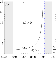
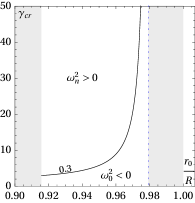
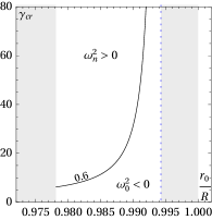
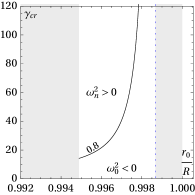
Figure 5: Stability of regular undercharged pressure stars. These stars are stars with $0<q^{2}<m^{2}$, also obey $0<\frac{q^{2}}{R^{2}}<1$, and belong to region (a) between lines $C_{0}$ and $C_{4}$ in Fig. 2. The critical adiabatic index $\gamma_{\rm cr}$ for four values of the electric charge parameter $\frac{q^{2}}{R^{2}}=0.1$, $\frac{q^{2}}{R^{2}}=0.3$, $\frac{q^{2}}{R^{2}}=0.6$, and $\frac{q^{2}}{R^{2}}=0.8$, is shown as a function of the radius $\frac{r_{0}}{R}$. In each of the four plots, the line starts at a minimum radius $\frac{r_{0}}{R}$ which correspond to a value $\gamma_{\rm cr}$ at some point on the curve $C_{0}$, and extends to relatively large values as $\frac{r_{0}}{R}$ grows and approaches the line $C_{4}$. The light gray region on the left side of each plot corresponds to stars that are not undercharged, and the light gray region on the right side of each plot corresponds to stars that are not regular and are beyond the Buchdahl-Andréasson limit.

The vertical dotted line on the right side of each of the four plots indicates the Buchdahl-Andréasson bound AndreassonQ , see also LemosZanchin2015 , which is represented by the curve $C_{4}$ in Fig. 2. The light gray region on the right side contains solutions for singular undercharged stars, i.e., undercharged configurations with higher radii, namely, the ones whose values of $\frac{r_{0}}{R}$ are on or above the curve $C_{4}$, i.e., in the region (f) in Fig. 2. Since they are singular undercharged star solutions they are of little interest in general and in particular for the stability analysis. The solid curved line in each of the four plots is for the vanishing fundamental oscillation frequency squared, i.e., for $\omega_{0}^{2}=0$, which means that $\omega_{0}^{2}$ changes sign across such a curve. All configurations represented by points located above the $\omega_{0}^{2}=0$ line are stable stars, i.e., all $\omega_{n}^{2}$ are positive, all configurations represented by points located below the $\omega_{0}^{2}=0$ line are unstable stars. Each solid curved line starts at some radius $\frac{r_{0}}{R}$ that corresponds to a point just outside the curve $C_{0}$ with a relatively low $\gamma_{\rm cr}$ and extends to some point $\frac{r_{0}}{R}$ on the curve $C_{4}$ at the Buchdahl-Andréasson bound where $\gamma_{\rm cr}$ diverges. For instance, the range of radii $\frac{r_{0}}{R}$ corresponding to regular undercharged stars for the case $\frac{q^{2}}{R^{2}}=0.3$ is from $\frac{r_{0}}{R}=0.915703$ to $\frac{r_{0}}{R}=0.979269$, where the numbers are approximate values, as can be confirmed from the top right panel of Fig. 5. Note that, for a fixed finite adiabatic index $\gamma$, the undercharged pressure stars are stable configurations against radial perturbations for relatively small radius, i.e., small $\frac{r_{0}}{R}$ which, since $R$ is a constant with the meaning of inverse effective energy density, means a normal star far from the Buchdahl-Andréasson bound and so far from forming a horizon. At the Buchdahl-Andréasson bound, these stars are unstable as they need an infinite $\gamma_{\rm cr}$.

In Fig. 6 we show the numerical results for the critical adiabatic index $\gamma_{\rm cr}$ but now as a function of the radius $\frac{r_{0}}{r_{+}}$, instead of $\frac{r_{0}}{R}$.

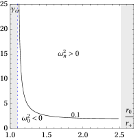
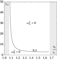
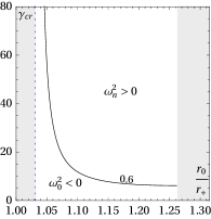
Figure 6: Stability of regular undercharged pressure stars. These stars are stars with $0<q^{2}<m^{2}$ and also obey $0<\frac{q^{2}}{R^{2}}<1$ and belong to region (a) between lines $C_{0}$ and $C_{4}$ in Fig. 2. The critical adiabatic index $\gamma_{\rm cr}$ for four values of the electric charge parameter $\frac{q^{2}}{R^{2}}=0.1$, $\frac{q^{2}}{R^{2}}=0.3$, $\frac{q^{2}}{R^{2}}=0.6$, and $\frac{q^{2}}{R^{2}}=0.8$, is shown as a function of the radius $\frac{r_{0}}{r_{+}}$. In each of the four plots, the line starts on the right at some radius $\frac{r_{0}}{r_{+}}$ on the line $C_{4}$ which corresponds to the Buchdahl-Andréasson bound and where $\gamma_{\rm cr}$ diverges, and extends to some $\frac{r_{0}}{r_{+}}$ on the line $C_{0}$ and where $\gamma_{\rm cr}$ has some positive given value. The light gray region on the left side of each plot corresponds to stars that are not regular and are beyond the Buchdahl-Andréasson limit, and the light gray region on the right side of each plot corresponds to stars that are not undercharged.

The radius $\frac{r_{0}}{r_{+}}$ helps in a better understanding of the compactness of the star, i.e., in the relation between the star radius $r_{0}$ and its gravitational radius $r_{+}$, which is now the quantity kept constant, rather than $R$. The critical adiabatic index $\gamma_{\rm cr}$ is shown for the same four values of the electric charge, namely, $\frac{q^{2}}{R^{2}}=0.1$, $\frac{q^{2}}{R^{2}}=0.3$, $\frac{q^{2}}{R^{2}}=0.6$, and $\frac{q^{2}}{R^{2}}=0.8$, as indicated in the figure. In each plot, the light gray region on the left side contains solutions for singular undercharged stars, i.e., undercharged configurations with small radii, namely, configurations for which the values of $\frac{r_{0}}{r_{+}}$ are on or above the curve $C_{4}$ in the region (f) of Fig. 2, and since they represent singular solutions, they are of little interest. The vertical dotted line in the left side of each of the four plots indicates the Buchdahl-Andréasson bound AndreassonQ , see also LemosZanchin2015 , which is represented by the curve $C_{4}$ in Fig. 2. The white region represents the range of the parameter $\frac{r_{0}}{r_{+}}$ where regular undercharged stars are found. The light gray region on the right side contains solutions that are overcharged stars, so require a different analysis. The solid curved line in each of the four plots is for the vanishing fundamental oscillation frequency squared, i.e., for $\omega_{0}^{2}=0$, which means that $\omega_{0}^{2}$ changes sign across such a curve. All configurations represented by points located above the $\omega_{0}^{2}=0$ line are stable stars, i.e., all $\omega_{n}^{2}$ are positive, all configurations represented by points located below the $\omega_{0}^{2}=0$ line are unstable stars. The solid curved line starts from the left at the curve $C_{4}$ at the Buchdahl-Andréasson bound where the stars are very compact and $\gamma_{\rm cr}$ diverges and extends to the right at some minimum for $\frac{r_{0}}{r_{+}}$ relatively large, that corresponds to a point on the curve $C_{0}$ where the stars are not anymore undercharged. Stability of stars with $\frac{r_{0}}{r_{+}}$ approaching the curve $C_{4}$, i.e., the Buchdahl-Andréasson bound occurs just for arbitrarily large values of the adiabatic index. For a fixed adiabatic index, the undercharged pressure stars are stable configurations against radial perturbations for relatively large radius, i.e., large $\frac{r_{0}}{r_{+}}$.

In Table 3 we give details of the numerical results for the stability of an undercharged star. The behavior of $\gamma_{\rm cr}$ as a function of the radius $\frac{r_{0}}{R}$ and $\frac{r_{0}}{r_{+}}$, for $\frac{q^{2}}{R^{2}}=0.3$, is displayed. The values of the critical adiabatic index $\gamma_{\rm cr}$ are obtained from the shooting and the pseudospectral methods, and are in agreement to each other up to six decimal places.

$\frac{r_{0}}{R}$	$\frac{r_{0}}{r_{+}}$	$\gamma_{\rm cr}$
$0.915704$	1.66855	$2.95794$
$0.924784$	1.39611	$3.32947$
$0.933863$	1.30128	$3.86695$
$0.942943$	1.23458	$4.70936$
$0.952022$	1.18179	$6.20193$
$0.961102$	1.13763	$9.47855$
$0.970181$	1.09943	$21.1295$
$0.979261$	1.06562	$440359$

Table 3: The critical adiabatic index $\gamma_{\rm cr}$ for the radial perturbations of undercharged stars with $\frac{q^{2}}{R^{2}}=0.3$ and for various values of the parameter $\frac{r_{0}}{R}$ and the compactness ratio $\frac{r_{0}}{r_{+}}$. These undercharged stars are in the region (a) of Fig. 2.

We have calculated the zero mode frequencies squared $\omega_{0}^{2}$ and the first mode frequencies squared $\omega_{1}^{2}$ for these $\frac{q^{2}}{R^{2}}=0.3$ stars with $\gamma=4$. We find that a star with $\frac{r_{0}}{R}=0.933863$ and so $\frac{r_{0}}{r_{+}}=1.3012$ has $\omega_{0}^{2}=2.34262\times 10^{-3}$, $\omega_{1}^{2}=0.541388$, and $\gamma_{\rm cr}=3.86695$, so $\gamma=4$ being above $\gamma_{\rm cr}$ this star is stable to radial perturbations, while a star with $\frac{r_{0}}{R}=0.942943$ and so $\frac{r_{0}}{r_{+}}=1.23458$ has $\omega_{0}^{2}=-0.01355012$, $\omega_{1}^{2}=0.628574$, and $\gamma_{\rm cr}=4.70936$, so $\gamma=4$ being below $\gamma_{\rm cr}$ this star is unstable. The solutions for these undercharged pressure stars having radii extending from approximately $\frac{r_{0}}{R}=0.915703$ to approximately $\frac{r_{0}}{R}=0.979269$, in the $\gamma=4$ adiabatic index case have $\omega_{0}^{2}$ positive in the range $0.915703\leq\frac{r_{0}}{R}\leq 0.942943$, where the values given are approximate values, and $\omega_{0}^{2}$ negative in the range $0.942943\leq\frac{r_{0}}{R}\leq 0.979269$, where the values given are approximate values, as it can be seen in more detail in Appendix E.

Undercharged stars that are singular, are stars with $q^{2}<m^{2}$ and also are above the Buchdahl-Andréasson curve $C_{4}$. These configurations belong to region (f), the region between the horizontal line $r_{0}=r_{+}=R$ and the line $C_{4}$ in Fig. 2. They are of no interest for the stability problem since the curvature scalars and the fluid quantities diverge at some radius inside the matter distribution.

IV.1.3 Extremally charged dust stars

Extremely charged dust stars or Bonnor stars lemoszanchin2008 are configurations that have charge density equal to mass density, $\rho_{e}=\rho$, the pressure is zero, obey $q^{2}=m^{2}$ and also obey $0<\frac{q^{2}}{R^{2}}<1$. These configurations are on the line $C_{0}$ in Fig. 2.

In this case, the energy density is positive and since the pressure is zero everywhere inside the matter one has $h(r)=\rho(r)+p(r)>0$. We can analyze the stability in this case directly, without having to resort to the theorem in Appendix C. Indeed, from Eqs. (35)-(40) one finds that since $\rho_{e}=\rho$ and $p=0$, one has $F(r)=0$, $G(r)=0$, and $H(r)=0$, and so Eq. (35) reduces to $\omega^{2}W(r)\zeta(r)=0$, i.e.,

$$\omega^{2}\rho(r)A^{\frac{3}{2}}(r)\xi(r)=0\,,$$ (68)

where we have used Eqs. (35) and (36). One can find Eq. (68) directly from Eq. (32). For generic $\rho(r)$, $A(r)$, and $\xi(r)$, the solution is

$$\omega^{2}=0\,.$$ (69)

Thus, extremely charged dust stars have a neutral stability against radial perturbations. If displaced in a spherically symmetric way they stay put or increase or decrease their radius homothetically and uniformly. An extremely charge dust star by itself neither expands nor collapses. Note, however, that for a nongeneric $A(r)$, namely, $A(r)=0$, for some $r$, than $\omega^{2}$ can be anything, we return to this case later.

Numerically, the behavior of this type of solutions against small radial perturbations can be displayed through the region (a) when the parameters of the stars in that region are very close to the line $C_{0}$. With an adiabatic index $\gamma=4$ and $\frac{q^{2}}{R^{2}}=0.3$ in the region (a), the frequencies are very close to zero for $\frac{r_{0}}{R}=0.915704$, i.e., near the line $C_{0}$, see also Appendix E. This implies that along the line $C_{0}$, the square frequencies for the fundamental and the first excited modes are very close to zero or vanish as Eq. (69) implies. This case has also been worked out in Omote1974 ; Glazer1976 .

IV.1.4 Overcharged tension stars

Overcharged regular tension stars are stars with $m^{2}<q^{2}$ and also obey $\frac{q^{2}}{R^{2}}<1$. These configurations belong to region (b), the region between lines $C_{0}$ and $C_{1}$ in Fig. 2.

In this case, the energy density is positive and the pressure is negative, it is a tension. The enthalpy density $h(r)=\rho(r)+p(r)$ is always greater than zero and, as a consequence, the function $W(r)$ that appears in Eq. (35) is positive. However, the sign of the function $F(r)$ depends on the product $\gamma p(r)$. Therefore, if $\gamma$ is assumed to be positive, the SL problem falls into the case (B) of the theorem summarized in Appendix C. The corresponding theorem implies that for a positive function $W(r)$ and a negative function $F(r)$, the sequence of eigenvalues is bounded from above, with fundamental frequency $\omega_{0}^{2}$ being the largest among all of them, i.e., $\cdots<\omega_{2}^{2}<\omega_{1}^{2}<\omega_{0}^{2}<\infty$. Hence, if the restriction $\gamma>\gamma_{\rm cr}>0$ is fulfilled, $\omega_{0}^{2}$ will be positive but the largest excited modes would have negative square frequencies and the configurations will be unstable against radial perturbations, see Appendix E for more details. Let us give physical arguments for the instability of these configurations when one considers $\gamma$ positive. Equation (25) can be cast as $\Delta p=c_{s}^{2}\Delta\rho$, where $c_{s}^{2}$ is the sound speed squared defined as $c_{s}^{2}=\dfrac{\gamma p}{\rho+p}$. In the interior region of tension stars the conditions $p<0$ and $\rho+p>0$ hold, implying that for $\gamma>0$ one has $c_{s}^{2}=\frac{\Delta p}{\Delta\rho}<0$, which means that when the density increases the tension increases and conversely when the density decreases the tension decreases. Then, when perturbing the system, if the fluid is compressed, and so the density increases, so also the tension grows, favoring the system to get even more compressed in a runaway process. Conversely, when perturbing the system, if the fluid is expanded, and so the density decreases, so also the tension diminishes, favoring the system to get even more expanded in a runaway process. This implies that, once started, the perturbed configuration never stops its process of compression or expansion, indicating an instability of the system. Another way of seeing this is that for $\gamma>0$, the sound speed squared obeys $c_{s}^{2}<0$, the sound speed is imaginary, and so there is no propagation of the perturbation and no possibility for stability. This leads to the conclusion that for tension stars, i.e., stars supported by negative pressure, one should assume that the radial perturbations are governed by a negative $\gamma$, and ask whether there are stable configurations for overcharged tension stars when $\gamma<0$ or not. If the adiabatic index $\gamma$ is negative, the coefficients $F(r)$ and $W(r)$ that appear in Eq. (35) are both positive functions, and so in the SL problem this leads to the case (A) of the theorem given in Appendix C. In this case the stable solutions are found for negative adiabatic index such that $\gamma<\gamma_{\rm cr}$, where negative $\gamma_{\rm cr}$ is the critical, i.e., maximum negative number, value of $\gamma$, or in terms of absolute value which makes things clearer, one has $|\gamma|>|\gamma_{\rm cr}|$ for stability. Let us give physical arguments for the possible stability of these configurations when one considers $\gamma$ negative. Equation (25), as we have already seen, can be cast as $\Delta p=c_{s}^{2}\Delta\rho$, where $c_{s}^{2}$ is the sound speed squared defined as $c_{s}^{2}=\dfrac{\gamma p}{\rho+p}$. In the interior region of tension stars the conditions $p<0$ and $\rho+p>0$ hold, implying that for $\gamma<0$ one has $c_{s}^{2}>0$. Moreover, now if the density increases the tension decreases, and conversely if the density decreases the tension increases. Then, when perturbing the system radially, if the fluid is compressed, and so the density increases, so the tension diminishes favoring the system to get less compressed in a possible stable process. Conversely, when perturbing the system radially, if the fluid is expanded, and so the density decreases, so the tension grows, favoring the system to get less expanded in a possible stable process. This implies that, once started, the perturbed configuration can return to the original configuration, the process of compression and expansion can be halted, indicating stability of the system. Another way of seeing this is that for $\gamma<0$, the sound speed squared obeys $c_{s}^{2}>0$, the sound speed is real, and so there is propagation of the perturbation and possibility for stability.

In Fig. 7, we show the numerical results for the critical adiabatic index $\gamma_{\rm cr}$, negative here, as a function of the radius $\frac{r_{0}}{R}$ for four values of $\frac{q^{2}}{R^{2}}$, namely, $\frac{q^{2}}{R^{2}}=0.06$, $\frac{q^{2}}{R^{2}}=0.32$, $\frac{q^{2}}{R^{2}}=0.60$, and $\frac{q^{2}}{R^{2}}=0.82$, i.e., for overcharged stars. In each plot, the light gray region on the left side is for solutions that are singular overcharged stars, i.e., stars beyond the curve $C_{1}$ of Fig. 2.

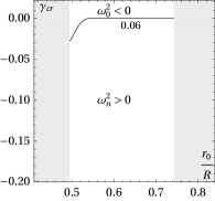
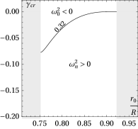
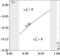
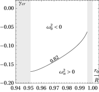
Figure 7: Stability of regular overcharged tension stars. These stars are stars with $m^{2}<q^{2}$ and also obey $0<\frac{q^{2}}{R^{2}}<1$ and belong to region (b) between lines $C_{0}$ and $C_{1}$ in Fig. 2. The critical adiabatic index $\gamma_{\rm cr}$ for four values of the electric charge parameter $\frac{q^{2}}{R^{2}}=0.06$, $\frac{q^{2}}{R^{2}}=0.32$, $\frac{q^{2}}{R^{2}}=0.60$, and $\frac{q^{2}}{R^{2}}=0.82$, is shown as a function of the radius $\frac{r_{0}}{R}$. In each of the four plots, the line starts at a minimum radius $\frac{r_{0}}{R}$ which correspond to a negative value $\gamma_{\rm cr}$ at some point on the curve $C_{1}$, and extends to some negative value as $\frac{r_{0}}{R}$ grows and approaches the line $C_{0}$. The light gray region on the left side of each plot corresponds to stars that are overcharged and singular, beyond the curve $C_{1}$, and the light gray region on the right side of each plot corresponds to stars that are not overcharged, beyond the curve $C_{0}$.

The white region represents the range of the parameter $\frac{r_{0}}{R}$ where regular overcharged stars are found. The light gray region on the right side contains solutions that are not overcharged, i.e., stars beyond the curve $C_{0}$, and do not belong here. The solid curved line in each of the four plots is for the vanishing fundamental oscillation frequency squared, i.e., for $\omega_{0}^{2}=0$, which means that $\omega_{0}^{2}$ changes sign across such a curve. All configurations represented by points located below the $\omega_{0}^{2}=0$ line are stable stars, i.e., all $\omega_{n}^{2}$ are positive, all configurations represented by points located above the $\omega_{0}^{2}=0$ line are unstable stars. Each solid curved line starts at some radius $\frac{r_{0}}{R}$ that corresponds to a point on the curve $C_{1}$ and corresponds to the first nonsingular overcharged stars on the curve, and extends to some point $\frac{r_{0}}{R}$ on the curve $C_{0}$ where the solutions have charge density equal to mass density. Along the solid line, from left to right as $\frac{r_{0}}{R}$ increases, the stars get more mass, and so need less tension to support the interior against expansion. For overcharged stars there is no gravitational radius $r_{+}$ and it means there is no possibility of interchanging $\frac{r_{0}}{R}$ with $\frac{r_{0}}{r_{+}}$. One could think in plotting the critical adiabatic index $\gamma_{\rm cr}$ as a function of $\frac{r_{0}}{m}$ instead, where $m$ is the spacetime mass, but there is no gain in it clearly, the only difference would be a reverse of the sign in the slope of the curve.

In Table 4 we give details of the numerical results for the stability of overcharged stars. The behavior of $\gamma_{\rm cr}$ as a function of the radius $\frac{r_{0}}{R}$ for $\frac{q^{2}}{R^{2}}=0.6$, is displayed. The values of the critical adiabatic index $\gamma_{\rm cr}$ are obtained from the shooting and pseudospectral methods, and are in agreement to each other to six decimal places. We have calculated the zero mode frequencies squared $\omega_{0}^{2}$ and the first mode frequencies squared $\omega_{1}^{2}$ for these $\frac{q^{2}}{R^{2}}=0.6$ stars with $\gamma=-0.06$. We find that for a star with $\frac{r_{0}}{R}=0.936112$ one has $\omega_{0}^{2}=-1.69590\times 10^{-3}$, and $|\gamma_{\rm cr}|=0.0623795$, so $|\gamma|=0.06$ being below $|\gamma_{\rm cr}|$ means that this star is unstable against radial perturbations, while for a star with $\frac{r_{0}}{R}=0.950112$ one has $\omega_{0}^{2}=5.03598\times 10^{-3}$, $\omega_{1}^{2}=0.0529323$, and $|\gamma_{\rm cr}|=0.0483227$, so $|\gamma|=0.06$ being above $|\gamma_{\rm cr}|$ means that this star is unstable.

$\frac{r_{0}}{R}$	$\gamma_{\rm cr}$
0.880113	-0.125874
0.894113	-0.113132
0.908113	-0.0952036
0.922113	-0.0779790
0.936112	-0.0623795
0.950112	-0.0483227
0.964112	-0.0352687
0.978111	-0.0220528

Table 4: The critical adiabatic index $\gamma_{\rm cr}$ for the radial perturbations of overcharged stars with $\frac{q^{2}}{R^{2}}=0.6$ and for various values of the parameter $\frac{r_{0}}{R}$. These overcharged stars are in the region (b) of Fig. 2.

The solutions for these overcharged tension stars having radii extending from approximately $\frac{r_{0}}{R}=0.880113$ to approximately $\frac{r_{0}}{R}=0.978111$ in the $\gamma=-0.06$ adiabatic index case, have $\omega_{0}^{2}$ negative approximately in the range $0.880113\leq\frac{r_{0}}{R}\leq 0.938387$, and $\omega_{0}^{2}$ positive approximately in the range $0.938387\leq\frac{r_{0}}{R}\leq 0.978111$. Thus, stars with larger $\frac{r_{0}}{R}$, i.e., overcharged stars with more mass and less electric charge, and thus less tension, are stable to radial perturbations. Moreover, for $\frac{r_{0}}{R}$ close to the line $C_{0}$ in the region (b) of Fig. 2, one has that the corresponding stars tend to electrically charged dust stars with $m^{2}=q^{2}$, the tension on these tension stars being very small. One finds numerically that $\omega_{0}^{2}$ as well as all other higher tones tend to zero and so in the limit these stars are neutrally stable, as we have discussed in the undercharged case and have found the exact stability solutions in the charge density equal energy density case. Some more detail is given in Appendix E. An interesting case needing further investigation occurs when $\frac{r_{0}}{R}\to 1$ and $\frac{q^{2}}{R^{2}}\to 1$ for the solutions in the region (b), see below.

Overcharged stars that are singular are stars with $m^{2}<q^{2}$ and also obey $\frac{q^{2}}{R^{2}}<\frac{27}{16}=1.6875$. These configurations belong to region (c), the region between lines $C_{1}$ and $C_{2}$ in Fig. 2. They are of no interest for the stability problem since the curvature scalars and the fluid quantities diverge at some radius inside the matter distribution.

IV.2 The stability of regular black holes

IV.2.1 Regular black holes with negative energy densities

Regular black holes with negative energy densities are also phantom regular black holes with no singularities, for which the electric charge obeys $\frac{q^{2}}{R^{2}}>0$, and the radius $r_{0}$ is inside the Cauchy horizon, $r_{0}<r_{-}$. These configurations belong to region (d1), i.e., to the right of lines $C_{2}$ and below the line $C_{31}$ plus $C_{31}C_{32}$ in Fig. 2.

In this case, the energy density $\rho(r)$ is negative for a range of the radial coordinate $r$ inside the matter and the pressure $p(r)$ is always negative. The enthalpy density $h(r)=\rho(r)+p(r)$ is everywhere less than zero, and as a consequence, assuming $\gamma>0$ the coefficients $F(r)$ and $W(r)$ that appear in Eq. (35) are both positive functions, and so in the SL problem this leads to the case (A) of the theorem given in Appendix C. Therefore stable solutions to radial perturbations of these regular black holes are found for positive adiabatic indices such that $\gamma>\gamma_{\rm cr}$.

In Fig. 8, we show the numerical results for the critical adiabatic index $\gamma_{\rm cr}$ as a function of the radius $\frac{r_{0}}{R}$ for four values of the electric charge, namely, $\frac{q^{2}}{R^{2}}=0.1$, $\frac{q^{2}}{R^{2}}=0.6$, $\frac{q^{2}}{R^{2}}=1.1$, and $\frac{q^{2}}{R^{2}}=1.6875$, as indicated in the figure, with the value $\frac{q^{2}}{R^{2}}=\frac{27}{16}=1.6875$ being the value of the elbow in curve $C_{2}$ of Fig. 2.

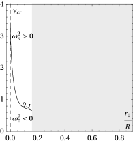
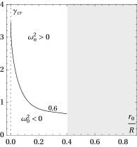
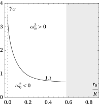
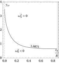
Figure 8: Stability of regular black holes with negative energy density. These regular black holes belong to region (d1) to the right of line $C_{2}$ and to the left of the vertical line $\frac{q^{2}}{R^{2}}=\frac{27}{16}=1.6875$ in Fig. 2. The critical adiabatic index $\gamma_{\rm cr}$ for four values of the electric charge parameter $\frac{q^{2}}{R^{2}}=0.1$, $\frac{q^{2}}{R^{2}}=0.6$, $\frac{q^{2}}{R^{2}}=1.1$, and $\frac{q^{2}}{R^{2}}=\frac{27}{16}=1.6875$, is shown as a function of the radius $\frac{r_{0}}{R}$. In each of the four plots, the line starts just above $\frac{r_{0}}{R}=0$ for some $\gamma_{\rm cr}$ and extends to some value as $\frac{r_{0}}{R}$ grows and approaches the line $C_{2}$. In each of the four plots, the adiabatic index $\gamma_{\rm cr}$ decreases up to some radius $\frac{r_{0}}{R}$ where, although not discernible in the plots, it starts to grow again slightly, the reason for this behavior being not clear. The light gray region on the right side of each plot corresponds to objects beyond the curve $C_{2}$, that are overcharged and singular, and are not black hole configurations.

In each plot the left part is the axis $\frac{r_{0}}{R}=0$. The white region represents the range of the parameter $\frac{r_{0}}{R}$ where regular black holes are found. The light gray region on the right side of each plot contains solutions of singular charged stars, i.e., overcharged configurations with higher radii, namely, the ones whose values of $\frac{r_{0}}{R}$ are on or above the curve $C_{2}$ of mass equal to charge, i.e., in the region (c) in Fig. 2, and so are of no interest. The solid curved line in each of the four plots is for the vanishing fundamental oscillation frequency squared, i.e., for $\omega_{0}^{2}=0$, which means that $\omega_{0}^{2}$ changes sign across such a curve. All configurations represented by points located above the $\omega_{0}^{2}=0$ line are stable regular black holes, i.e., all $\omega_{n}^{2}$ are positive, all configurations represented by points located below the $\omega_{0}^{2}=0$ line are unstable regular black holes. Each solid curved line starts just above $\frac{r_{0}}{R}=0$ and extends to some point $\frac{r_{0}}{R}$ on the curve $C_{2}$. One sees that the critical adiabatic index $\gamma_{\rm cr}$ on each line of the four different $\frac{q^{2}}{R^{2}}$, starts at approximately the same value for $\frac{r_{0}}{R}$ very small, and then decreases for larger $\frac{r_{0}}{R}$. One can make some further remarks for all the four plots with the numbers given meaning approximate rather than exact numbers. In each of the four plots the critical adiabatic index decreases to a minimum value close to $\gamma_{\rm cr}=0.66$ for relatively large $\frac{r_{0}}{R}$, and then grows again, although only a little not visible in the plots, to approximately $\gamma_{\rm cr}=0.6667$ when $\frac{r_{0}}{R}$ approaches the line $C_{2}$, i.e., the line $m^{2}=q^{2}$. For a fixed adiabatic index $\gamma$ above about $\gamma_{\rm cr}=3.5$, all regular black holes are stable to radial perturbations. In each of the four plots, the line starts immediately after $\frac{r_{0}}{R}=0$ for some $\gamma_{\rm cr}$ and decreases up to some radius $\frac{r_{0}}{R}$ where it starts to grow again slightly. We have not been able to give a heuristic explanation for the reason of this change of stability in each of the four plots. For fixed adiabatic index $\gamma$ in the range $\gamma<0.6$ all regular black holes are unstable. In the limit $\frac{r_{0}}{R}=0$, the mass diverges, the metric turns into a Kasner metric, and the stability problem set here does not apply.

In Table 5, we give details of the numerical results for the stability of regular black holes with negative energy densities. The behavior of $\gamma_{\rm cr}$ as a function of the radius $\frac{r_{0}}{R}$, for $\frac{q^{2}}{R^{2}}=\frac{27}{16}=1.6875$, is displayed. The values of the critical adiabatic index $\gamma_{\rm cr}$ are obtained from the shooting and the pseudospectral methods, and are in agreement to each other up to six decimal places.

$\frac{r_{0}}{R}$	$\gamma_{\rm cr}$
0.0186989	2.59470
0.139572	1.30905
0.260445	0.916685
0.381318	0.766649
0.502191	0.701179
0.623064	0.670727
0.743937	0.659659
0.864810	0.666663

Table 5: The critical adiabatic index $\gamma_{\rm cr}$ for the radial perturbations of regular black holes with negative energy densities with $\frac{q^{2}}{R^{2}}=\frac{27}{16}=1.6875$ and for various values of the parameter $\frac{r_{0}}{R}$. These regular black holes are in the left part of region (d1) of Fig. 2.

We have calculated the zero mode frequencies squared $\omega_{0}^{2}$ and the first mode frequencies squared $\omega_{1}^{2}$ for these $\frac{q^{2}}{R^{2}}=\frac{27}{16}$ regular black holes with negative energy densities for the adiabatic index $\gamma=4$. We find that all these regular black holes are stable, all eigenfrequencies squared are positive. The solutions for these regular black holes have radii extending from above $\frac{r_{0}}{R}=0$ to approximately $\frac{r_{0}}{R}=0.866025$. Note that as $\frac{r_{0}}{R}$ increases the value of $\gamma_{\rm cr}$ decreases up to approximately $\frac{r_{0}}{R}=0.66$ where it increases again. All this can be seen in more detail in Appendix E.

In Fig. 9, we show the numerical results for the critical adiabatic index $\gamma_{\rm cr}$ as a function of the radius

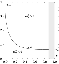
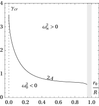
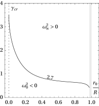
Figure 9: Stability of regular black holes with negative energy density, continuation from the previous figure. These regular black holes belong to region (d1) to the right of the vertical line $\frac{q^{2}}{R^{2}}=\frac{27}{16}=1.6875$, below the line $C_{31}$ plus $C_{31}C_{32}$, and to the left of the vertical line $\frac{q^{2}}{R^{2}}=3.0$ in Fig. 2. The critical adiabatic index $\gamma_{\rm cr}$ for four values of the electric charge parameter $\frac{q^{2}}{R^{2}}=1.8$, $\frac{q^{2}}{R^{2}}=2.4$, $\frac{q^{2}}{R^{2}}=2.7$, and $\frac{q^{2}}{R^{2}}=3.0$, is shown as a function of the radius $\frac{r_{0}}{R}$. In each of the four plots, the line starts just above $\frac{r_{0}}{R}=0$ for some $\gamma_{\rm cr}$ and extends to some value as $\frac{r_{0}}{R}$ grows and approaches the line $C_{31}$ plus $C_{31}C_{32}$. The adiabatic index $\gamma_{\rm cr}$ decreases up to some large $\frac{r_{0}}{R}$ and it decays abruptly for large $\frac{r_{0}}{R}$ being even zero when $\frac{q^{2}}{R^{2}}=3.0$, which is consistent since in this case the regular black hole is made of a pure de Sitter interior, and the de Sitter solution is stable against radial perturbations. The light gray region on the right side of each plot corresponds to different regular black holes, beyond the line $C_{31}$ plus $C_{31}C_{32}$.

$\frac{r_{0}}{R}$ for four values of the electric charge, namely, $\frac{q^{2}}{R^{2}}=1.8$, $\frac{q^{2}}{R^{2}}=2.4$, $\frac{q^{2}}{R^{2}}=2.7$, and $\frac{q^{2}}{R^{2}}=3.0$, as indicated in the figure. In each plot the left part is the axis $\frac{r_{0}}{R}=0$. The white region represents the range of the parameter $\frac{r_{0}}{R}$ where regular black holes are found. The light gray region on the right side contains solutions that do not belong here, the solutions correspond to different regular black holes, namely, the ones whose values of $\frac{r_{0}}{R}$ are on or above the curve $C_{31}$ plus $C_{31}C_{32}$, i.e., in the regions (d2), (e1), and (e2) in Fig. 2, with (e2) only appearing explicitly in Fig. 2. The solid curved line in each of the four plots is for the vanishing fundamental oscillation frequency squared, i.e., for $\omega_{0}^{2}=0$, which means that $\omega_{0}^{2}$ changes sign across such a curve. All configurations represented by points located above the $\omega_{0}^{2}=0$ line are stable regular black holes, i.e., all $\omega_{n}^{2}$ are positive, all configurations represented by points located below the $\omega_{0}^{2}=0$ line are unstable regular black holes. Each solid curved line starts just above $\frac{r_{0}}{R}=0$ and extends to some point $\frac{r_{0}}{R}$ on the curve $C_{31}$ plus $C_{31}C_{32}$. The four plots fall within the range $\frac{q^{2}}{R^{2}}>\frac{27}{16}$, so are to the right of the elbow in curve $C_{2}$. In all the four cases, for a fixed adiabatic index $\gamma$ above about $\gamma_{\rm cr}=3.5$, all regular black holes are stable against radial perturbations. For a fixed adiabatic index $\gamma$ below about $\gamma_{\rm cr}=3.5$, there are stable regular black holes for $\frac{r_{0}}{R}$ greater than some value. For small $\frac{r_{0}}{R}$ the behavior of $\gamma_{\rm cr}$ is practically the same for each of the four plots. For large $\frac{r_{0}}{R}$ the decrease in $\gamma_{\rm cr}$ is very rapid, abrupt in some cases, when the radius $\frac{r_{0}}{R}$ approaches the curve $C_{31}$ plus $C_{31}C_{32}$. In the case $\frac{q^{2}}{R^{2}}=3.0$ and in the limit $\frac{r_{0}}{R}=1$, the critical adiabatic index indeed vanishes, and the regular black hole is stable independently of the $\gamma$, it is absolutely stable to these perturbations. This is because this case is of a regular black hole made of an interior which is purely de Sitter up to the boundary which is at the Cauchy horizon radius, $r_{0}=r_{-}$, where, in turn, there is a massless electric coat LemosZanchin2011 , and as it is known the de Sitter solution is stable.

In Table 6, we give details of the numerical

$\frac{r_{0}}{R}$	$\gamma_{\rm cr}$
0.0186989	2.71551
0.158885	1.42949
0.299070	1.00152
0.439256	0.817217
0.579442	0.723642
0.719628	0.667765
0.859813	0.616897
0.999999	0.000367

Table 6: The critical adiabatic index $\gamma_{\rm cr}$ for the radial perturbations of regular black holes with negative energy densities with $\frac{q^{2}}{R^{2}}=3$ and for various values of the parameter $\frac{r_{0}}{R}$. These regular black holes are in a part of region (d1) of Fig. 2.

results for the stability of regular black holes with negative energy densities. The behavior of $\gamma_{\rm cr}$ as a function of the radius $\frac{r_{0}}{R}$, for $\frac{q^{2}}{R^{2}}=3$, is displayed. The values of the critical adiabatic index $\gamma_{\rm cr}$ are obtained from the shooting and the pseudospectral methods, and are in agreement to each other up to six decimal places. The solutions for these regular black holes have radii extending from above $\frac{r_{0}}{R}=0$ to $\frac{r_{0}}{R}=1$. Note that as $\frac{r_{0}}{R}$ increases the $\gamma_{\rm cr}$ decreases up to zero when $\frac{r_{0}}{R}$ is equal to one, so that this regular black hole is stable for this type of perturbations.

In Fig. 10, we show the numerical results for the

Figure 10: Stability of regular black holes with negative energy density, continuation from the previous figures, i.e., Figs. 8 and 9. These regular black holes belong to region (d1) to the right of the vertical line $\frac{q^{2}}{R^{2}}=3$ and have as upper boundary the line $r_{0}=r_{-}=R$ in Fig. 2. The critical adiabatic index $\gamma_{\rm cr}$ for four values of the electric charge parameter $\frac{q^{2}}{R^{2}}=3.1$, $\frac{q^{2}}{R^{2}}=5.0$, $\frac{q^{2}}{R^{2}}=10$, and $\frac{q^{2}}{R^{2}}=20$, is shown as a function of the radius $\frac{r_{0}}{R}$. In each of the four plots, the line starts just above $\frac{r_{0}}{R}=0$ for some $\gamma_{\rm cr}$ and extends to some value as $\frac{r_{0}}{R}$ grows and approaches the line $r_{0}=r_{-}=R$. The adiabatic index $\gamma_{\rm cr}$ decreases up to some large $\frac{r_{0}}{R}$ and in the last three plots it starts to grow for large $\frac{r_{0}}{R}$ reaching a finite value at the $\frac{r_{0}}{R}=1$.

critical adiabatic index $\gamma_{\rm cr}$ as a function of the radius $\frac{r_{0}}{R}$ for four values of the electric charge, namely, $\frac{q^{2}}{R^{2}}=3.1$, $\frac{q^{2}}{R^{2}}=5$, $\frac{q^{2}}{R^{2}}=10$, and $\frac{q^{2}}{R^{2}}=20$, as indicated in the figure. In each plot the left part is the axis $\frac{r_{0}}{R}=0$. The white region represents the range of the parameter $\frac{r_{0}}{R}$ where regular black holes are found, all situated in the region (d1) in Fig. 2. The right part is the axis $\frac{r_{0}}{R}=1$. The solid curved line in each of the four plots is for the vanishing fundamental oscillation frequency squared, i.e., for $\omega_{0}^{2}=0$, which means that $\omega_{0}^{2}$ changes sign across such a curve. All configurations represented by points located above the $\omega_{0}^{2}=0$ line are stable regular black holes, i.e., all $\omega_{n}^{2}$ are positive, all configurations represented by points located below the $\omega_{0}^{2}=0$ line are unstable regular black holes. Each solid curved line starts just above $\frac{r_{0}}{R}=0$ and extends to a point on the line $\frac{r_{0}}{R}=\frac{r_{-}}{R}=1$. The limit $\frac{r_{0}}{R}\to 1$ with $\frac{q^{2}}{R^{2}}>3$ gives the top boundary of region (d1) of Fig. 2. For small $\frac{r_{0}}{R}$ the behavior of $\gamma_{\rm cr}$ is practically the same for each of the four plots, it starts at about $\gamma_{\rm cr}=3.5$. For large $\frac{r_{0}}{R}$ and $\frac{q2}{R^{2}}$ a little larger than $3$, $\frac{q2}{R^{2}}=3.1$ in the plot, $\gamma_{\rm cr}$ decreases to some value greater than zero when $\frac{r_{0}}{R}\to 1$. For large $\frac{r_{0}}{R}$ and $\frac{q2}{R^{2}}$ relatively large, as is shown in the plots for $\frac{q^{2}}{R^{2}}=5$, $\frac{q^{2}}{R^{2}}=10$, and $\frac{q^{2}}{R^{2}}=20$, the increase in $\gamma_{\rm cr}$ is very rapid, even abrupt, when the radius $\frac{r_{0}}{R}$ approaches $\frac{r_{0}}{R}=1$. In this limit, the regular black holes are stable against radial perturbations for positive adiabatic indices larger than some $\gamma_{\rm cr}$. This $\gamma_{\rm cr}$ increases with the electric charge, starting from $\gamma_{\rm cr}=0$ at $\frac{q2}{R^{2}}=3$, and diverges in the limit $\frac{q^{2}}{R^{2}}\to\infty$.

In Table 7, we give details of the numerical

$\frac{r_{0}}{R}$	$\gamma_{\rm cr}$
0.0186989	2.81135
0.158885	1.62442
0.299070	1.16791
0.439256	0.941473
0.579442	0.813839
0.719628	0.729194
0.859813	0.656414
0.999999	1.86624

Table 7: The critical adiabatic index $\gamma_{\rm cr}$ for the radial perturbations of regular black holes with negative energy densities with $\frac{q^{2}}{R^{2}}=5$ and for various values of the parameter $\frac{r_{0}}{R}$. These regular black holes are in right part of region (d1) of Fig. 2.

results for the stability of regular black holes with negative energy densities. The behavior of $\gamma_{\rm cr}$ as a function of the radius $\frac{r_{0}}{R}$, for $\frac{q^{2}}{R^{2}}=5$, is displayed. The values of the critical adiabatic index $\gamma_{\rm cr}$ are obtained from the shooting and the pseudospectral methods, and are in agreement to each other up to six decimal places. The solutions for these regular black holes have boundary radii extending from above $\frac{r_{0}}{R}=0$ to approximately $\frac{r_{0}}{R}=1$. Note that as $\frac{r_{0}}{R}$ increases the index $\gamma_{\rm cr}$ decreases to a minimum at some $\frac{r_{0}}{R}$ close to $\frac{r_{0}}{R}=1$, and then increases with $\frac{r_{0}}{R}$ up to a finite value in the limit $\frac{r_{0}}{R}\to 1$. The change of behavior of $\gamma_{\rm cr}$ in comparison to the region for smaller electric charges occurs exactly at $\frac{q^{2}}{R^{2}}=3$. Such a change is not visible in the case of $\frac{q^{2}}{R^{2}}=3.1$, whose $\gamma_{\rm cr}$ curve is shown in the top left panel of Fig. 10, because the turning point is very close to the boundary line.

IV.2.2 Regular black holes with a phantom matter core

Regular black holes with a phantom matter core have no singularities and the radius $r_{0}$ is inside the Cauchy horizon, $r_{0}<r_{-}$. These configurations belong to regions (d2) and (e1) above the curve $C_{31}$ plus $C_{31}C_{32}$ in Fig. 2 and below the line $C_{33}$ of Fig. 2, with Fig. 2 being an enlargement of Fig. 2 in that region of interest.

In the region (d2) the energy density is positive and finite at the center of the distribution of matter, changes to negative values at some $r<r_{0}$, and changes back to positive values close to the surface, the pressure is negative and, in modulus is larger than the energy density at the center of the distribution, and it goes to zero at the surface $r_{0}$. In the region (e1) the energy density is positive everywhere inside matter and the pressure is negative. Thus, for a finite region inside the matter one finds $\rho+p<0$. As a consequence, the coefficient $F(r)$ is a negative function on the whole interval $0\leq r\leq r_{0}$ if $\gamma$ is a positive number, and is a positive function on the whole interval $0\leq r\leq r_{0}$ if $\gamma$ is a negative number. The coefficient $W(r)$ is a negative function in $0\leq r\leq r_{d}$, for some $r_{d}$, and it is positive in $r_{d}\leq r\leq r_{0}$. This case falls into case (D) of the theorem in the Appendix C, and the behavior of the eigenvalues of the SL problem is tortuous. The upshot is that there are no stable configurations against radial perturbations for regular black holes with a phantom matter core, as it can be seen in more detail in Appendix E.

IV.2.3 Regular tension black holes with positive enthalpy density

Regular tension black holes with positive enthalpy density are not phantom and obey $r_{0}<r_{-}$. These configurations belong to region (e2), above the curve $C_{33}$ of Fig. 2 which is an enlargement of Fig. 2 to precisely see this region.

In this case, the energy density is positive everywhere inside the matter and the pressure is negative, i.e., the matter is constrained from bursting by tension. The enthalpy density is always positive $h(r)=\rho(r)+p(r)>0$. Since $h(r)>0$ one has that the coefficient $W(r)$ is a positive function. Thus, the SL problem falls into the case (A) of the theorem of Appendix C only if the adiabatic index is a negative number. In this case the stable solutions to radial perturbations are found for $\gamma<\gamma_{\rm cr}$ where $\gamma_{\rm cr}$ here is a negative number, so in absolute values $|\gamma|>|\gamma_{\rm cr}|$.

In Fig. 11 we show the numerical results for the critical adiabatic index $\gamma_{\rm cr}$ as a function of the radius for four values of the electric charge, namely, $\frac{q^{2}}{R^{2}}=1.1$, $\frac{q^{2}}{R^{2}}=2.2$, $\frac{q^{2}}{R^{2}}=2.8$, and $\frac{q^{2}}{R^{2}}=2.99$, as indicated in the figure.

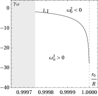
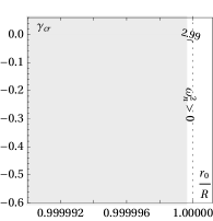
Figure 11: Stability of regular tension black holes with positive enthalpy density. These regular black holes belong to region (e2), above the curve $C_{33}$ of Fig. 2 which is an enlargement of Fig. 2. The critical adiabatic index $\gamma_{\rm cr}$ for four values of the electric charge parameter $\frac{q^{2}}{R^{2}}=1.1$, $\frac{q^{2}}{R^{2}}=2.2$, $\frac{q^{2}}{R^{2}}=2.8$, and $\frac{q^{2}}{R^{2}}=2.99$, is shown as a function of the radius $\frac{r_{0}}{R}$. In each of the four plots, the line starts at a minimum radius $\frac{r_{0}}{R}$ on the curve $C_{33}$ for which $\gamma_{\rm cr}$ is negative and for larger $\frac{r_{0}}{R}$, $\gamma_{\rm cr}$ becomes more negative up to the line $\frac{r_{0}}{R}=1$. The light gray region on the left side of each plot corresponds to other different regular tension black holes.

In each plot the light gray region on the left side contains solutions that are regular black holes but not of this kind, they are solutions below line $C_{33}$. The white region represents the range of the parameter $\frac{r_{0}}{R}$ where regular tension black holes with positive enthalpy density are found. The vertical line $\frac{r_{0}}{R}=1$ on the right side marks the end of the plots. The solid curved line in each of the four plots is for the vanishing fundamental oscillation frequency squared, i.e., for $\omega_{0}^{2}=0$, which means that $\omega_{0}^{2}$ changes sign across such a curve. All configurations represented by points located below the $\omega_{0}^{2}=0$ line are stable regular black holes against radial perturbations, i.e., all $\omega_{n}^{2}$ are positive, all configurations represented by points located above the $\omega_{0}^{2}=0$ line are unstable regular black holes. Each solid curved line starts at some $\frac{r_{0}}{R}$ and extends to $\frac{r_{0}}{R}=1$. The behavior of the critical adiabatic index $\gamma_{\rm cr}$ is such that it decreases slowly for relatively small radius, but then it decreases very fast when $\frac{r_{0}}{R}$ is near 1. So, in modulus, $|\gamma_{\rm cr}|$ is small for relatively low $\frac{r_{0}}{R}$ close to the curve $C_{33}$, and the maximum values of $|\gamma_{\rm cr}|$ in modulus are obtained for $\frac{r_{0}}{R}=1$, when $r_{0}$ is also equal to $r_{-}$. Note also that, for a fixed negative adiabatic index, the regular black hole configurations are stable for relatively small radius, but are unstable for large radius. In the $\frac{q^{2}}{R^{2}}$ near 1 case, of which $\frac{q^{2}}{R^{2}}=1.1$ shown is an example, for $\frac{r_{0}}{R}$ close to 1 stability is only achieved for large values of the adiabatic index $\gamma_{\rm cr}$, near $\gamma_{\rm cr}=-29$. In the $\frac{q^{2}}{R^{2}}$ far from 1 case, of which $\frac{q^{2}}{R^{2}}=2.8$ shown is an example, for $\frac{r_{0}}{R}$ close to 1 stability is now achieved for relatively small values of the adiabatic index $\gamma_{\rm cr}$, near $\gamma_{\rm cr}=-0.34$. In the limit $\frac{q^{2}}{R^{2}}\to 3$, i.e., approaching point $D$ of Figs. 2 and 2, of which $\frac{q^{2}}{R^{2}}=2.99$ is the closest value the numerical methods furnish good results, stability is achieved for all values of the adiabatic index $\gamma_{\rm cr}<0$, since $\gamma_{\rm cr}\to 0$. The limit $\frac{r_{0}}{R}=1$ with the electric charge in the interval $1<\frac{q^{2}}{R^{2}}<3$ gives the top boundary of region (e2) of Fig. 2. As seen in Fig. 11, in this limit, the regular tension black holes with positive enthalpy are stable against radial perturbations for negative adiabatic indices smaller than $\gamma_{\rm cr}$. The critical adiabatic index decreases in modulus with the electric charge, starting from arbitrarily large negative values close to $\frac{q^{2}}{R^{2}}=1$, i.e., at the QNBH configuration, and reaching $\gamma_{\rm cr}=0$ at $\frac{q2}{R^{2}}=3$, i.e., at the de Sitter regular black hole mentioned already.

In Table 8,

$\frac{r_{0}}{R}$	$\gamma_{\rm cr}$
0.998379	-0.327587
0.998610	-0.368522
0.998842	-0.416910
0.999073	-0.475289
0.999305	-0.549655
0.999536	-0.651395
0.999768	-0.819164
0.999999	-2.02034

Table 8: The critical adiabatic index $\gamma_{\rm cr}$ for the radial perturbations of regular black holes with positive enthalpy density with $\frac{q^{2}}{R^{2}}=2.2$ and for various values of the parameter $\frac{r_{0}}{R}$. These regular black holes are in region (e2) of Fig. 2 which is an enlargement of Fig. 2.

we give details of the numerical results for the stability of regular black holes with positive enthalpy density. The behavior of $\gamma_{\rm cr}$ as a function of the radius $\frac{r_{0}}{R}$, for $\frac{q^{2}}{R^{2}}=2.2$, is displayed. The values of the critical adiabatic index $\gamma_{\rm cr}$ are obtained from the shooting and the pseudospectral methods, and are in agreement to each other up to six decimal places. The solutions for these regular black holes are in the region (e2) of Fig. 2 and have boundary radii extending from relatively high $\frac{r_{0}}{R}$ up to $\frac{r_{0}}{R}=1$. Note that as $\frac{r_{0}}{R}$ increases the index $\gamma_{\rm cr}$ decreases negatively, i.e, its modulus $|\gamma_{\rm cr}|$ increases up to a maximum finite value. So the regular black holes in this region can be stable to radial perturbations.

IV.2.4 Regular de Sitter black hole: $r_{0}=r_{-}$ and $\frac{q^{2}}{R^{2}}=3$

Point $D$ in Fig. 2 is a special configuration, a pure de Sitter interior solution that obeys the equation of state $p(r)=-\rho(r)$ up to the lightlike surface boundary $r_{0}=r_{-}$, where there is a coat of electric charge, and where both the energy density and the pressure drop to zero. The solution is a regular black hole with a de Sitter interior and a lightlike boundary, and is a particular case of the regular black holes studied in LemosZanchin2011 .

This regular de Sitter black hole is stable, it has $\gamma_{\rm cr}=0$. The vanishing of $\gamma_{\rm cr}$ when approaching the point $D$ can be seen in the bottom right panel of Fig. 9, where the curve for $\gamma_{\rm cr}$ was drawn by taking $\frac{q^{2}}{R^{2}}=3.0$. The same behavior is verified in the top left panel of Fig. 10, where the curve for $\gamma_{\rm cr}$ was drawn by taking $\frac{q^{2}}{R^{2}}=3.1$, as well as in the bottom right panel of Fig. 11, where the curve for $\gamma_{\rm cr}$ was drawn by taking $\frac{q^{2}}{R^{2}}=2.99$. Our analysis confirms the previous studies on the stability of regular black holes with a de Sitter core inferred in Uchikata:2012zs . Moreover, we give a definite answer, that this de Sitter regular black hole is stable against radial perturbations.

IV.3 The stability of quasiblack holes and quasinonblack holes

IV.3.1 Quasiblack holes from regular undercharged pressure stars

QBHs from regular undercharged pressure stars are obtained by approaching the point $Q$ from region (a) of Fig. 2, obey $q^{2}=m^{2}$ and also obey $\frac{q^{2}}{R^{2}}=1$.

The resulting objects are pressure QBHs that satisfy all the energy conditions and, as long as the parameter $a$ obeys $1<a<\frac{4}{3}$, they also satisfy the causality condition LemosZanchin2010 .

In Fig. 12 we show the numerical results for the

Figure 12: Stability of QBHs from regular undercharged pressure stars. These QBHs come from approaching point Q from region (a) in Fig. 2. The critical adiabatic index $\gamma_{\rm cr}$ for four values of the parameter $a$, namely, $a=1.001$, $a=1.100$, $a=1.200$, and $a=\frac{4}{3}=1.333$, is shown as a function of the radius $\frac{r_{0}}{R}$. Each line starts at $\frac{r_{0}}{R}=0.9999$ and ends at $\frac{r_{0}}{R}=0.9999999$. The limit $\frac{r_{0}}{R}=1$ represents QBH configurations. The critical adiabatic index $\gamma_{\rm cr}$ diverges in this limit.

critical adiabatic index $\gamma_{\rm cr}$ as a function of the radius $\frac{r_{0}}{R}$ for four values of the parameter $a$, namely, $a=1.001$, $a=1.100$, $a=1.200$, and $a=\frac{4}{3}=1.333$, as indicated in the figure. The solid curved line in each of the four plots is for the vanishing fundamental oscillation frequency squared, i.e., for $\omega_{0}^{2}=0$, which means that $\omega_{0}^{2}$ changes sign across such a curve. All configurations represented by points located above the $\omega_{0}^{2}=0$ line are stable pressure stars, i.e., all $\omega_{n}^{2}$ are positive, all configurations represented by points located below the $\omega_{0}^{2}=0$ line are unstable pressure stars. For $\frac{r_{0}}{R}$ close to 1, i.e., on the QBH limit, one finds that to be stable to radial perturbations the adiabatic index has to be arbitrarily large. Thus, the QBH configurations which are obtained by approaching the point $Q$ from region (a) are unstable unless $\gamma$ assumes arbitrarily large values.

In Table 9 we give details of the numerical results

$a$	$\frac{q^{2}}{R^{2}}$	$\frac{m}{R}$	$\gamma_{\rm cr}$
1.001	0.999105	0.999552	3859.97
1.100	0.999062	0.999531	4329.59
1.200	0.999020	0.999510	4865.11
1.333	0.998967	0.999484	5689.66

Table 9: The critical adiabatic index $\gamma_{\rm cr}$ for radial perturbations of undercharged pressure stars, i.e., stars in region (a) of Fig. 2, for four values of the parameter $a$ close to the QBH configuration, i.e., for $\frac{r_{0}}{R}=0.9999999$. In the QBH limit, $\frac{r_{0}}{R}=1$, $\gamma_{\rm cr}$ diverges.

for the stability of QBHs from regular undercharged pressure stars. The behavior of $\gamma_{\rm cr}$ as a function of $a$, $\frac{q^{2}}{R^{2}}$, and $\frac{m}{R}$ is given for the configuration approaching the QBH limit. One sees that $\gamma_{\rm cr}$ is high and in the limit diverges.

IV.3.2 Quasiblack holes from extremal dust stars

QBHs from extremal dust stars are obtained by approaching the point $Q$ along the curve $C_{0}$ of Fig. 2, obey $a=1$, $q^{2}=m^{2}$, and also obey $\frac{q^{2}}{R^{2}}=1$.

The resulting objects have charge density equal to mass density, $\rho_{e}=\rho$, the pressure is zero and satisfy all the energy conditions and the causality condition lemosluz2021 , see also LemosZanchin2010 . These are extremal dust QBHs.

As we have seen in Eq. (68) the condition for stability of the stars along the $C_{0}$ curve is $\omega^{2}\rho(r)A^{\frac{3}{2}}(r)\xi(r)=0$. This means that for nonzero $A$ one has $\omega^{2}=0$ and the corresponding stars are neutrally stable. Now, for a QBH $A$ is zero at one radius, the gravitational radius $r_{+}$, which obeys $A(r_{+})=0$. So $A(r_{+})$ is zero at $r_{+}$ and nonzero for all other points. So $\omega^{2}=0$ for all radii except conceivably at $r_{+}$. But by continuity we must infer that $\omega^{2}=0$ for all radii. This result confirms what is otherwise known, namely, that these QBHs from extremal dust stars are topological objects lzjmp , and so stable to perturbations, in particular are neutrally stable against radial perturbations which is a remarkable result.

IV.3.3 Quasiblack holes from overcharged tension stars

QBHs from regular overcharged tension stars are obtained by approaching the point $Q$ from region (b) of Fig. 2, obey $0<a<1$, $q^{2}=m^{2}$, and also obey $\frac{q^{2}}{R^{2}}=1$.

The resulting objects are tension QBHs and satisfy all the energy conditions.

In Fig. 13 we show the numerical results for the critical adiabatic index $\gamma_{\rm cr}$ as a function of the radius $\frac{r_{0}}{R}$ for four values of the parameter $a$, namely, $a=0.06$, $a=0.24$, $a=0.60$, and $a=0.98$, as indicated in the figure. The solid curved line in each of the four plots is for the vanishing fundamental oscillation frequency squared, i.e., for $\omega_{0}^{2}=0$, which means that $\omega_{0}^{2}$ changes sign across such a curve. All configurations represented by points located below the $\omega_{0}^{2}=0$ line are stable tension stars, i.e., all $\omega_{n}^{2}$ are positive, all configurations represented by points located above the $\omega_{0}^{2}=0$ line are unstable tension stars. For $\frac{r_{0}}{R}$ close to 1, one sees that to be stable to radial perturbations the critical adiabatic index, $\gamma_{\rm cr}$, is negative, and has an almost constant value. In the limit of $\frac{r_{0}}{R}=1$, with $0<a<1$, i.e., at the QBH limit from tension stars, all $|\gamma_{\rm cr}|$ are finite. Thus, the QBH configurations which are obtained by approaching the point $Q$ from region (b) are stable to radial perturbations for a sufficiently moderate $|\gamma_{\rm cr}|$.

Figure 13: Stability of QBHs from regular overcharged tension stars. These QBHs come from approaching point $Q$ from region (b) in Fig. 2. The critical adiabatic index $\gamma_{\rm cr}$ for four values of the parameter $a$, namely, $a=0.06$, $a=0.24$, $a=0.60$, and $a=0.98$, is shown as a function of the radius $\frac{r_{0}}{R}$. Each line starts at $\frac{r_{0}}{R}=0.9999$ and end sat $\frac{r_{0}}{R}=0.9999999$. The limit $\frac{r_{0}}{R}=1$ represents QBH configurations. The critical adiabatic index $\gamma_{\rm cr}$ is negative and for a sufficiently high $|\gamma_{\rm cr}|$ these QBHs are stable against radial perturbations.

In Table 10 we give details of the numerical results for

$a$	$\frac{q^{2}}{R^{2}}$	$\frac{m}{R}$	$\gamma_{\rm cr}$
0.06	0.999781	0.999890	-0.165394
0.24	0.999562	0.999781	-0.135874
0.60	0.999307	0.999653	-0.113167
0.98	0.999115	0.999557	-0.0975539

Table 10: The critical adiabatic index $\gamma_{\rm cr}$ for radial perturbations of overcharged tension stars, i.e., stars in region (b) of of Fig. 2, for four values of the parameter $a$ close to the QBH configuration, i.e., for $\frac{r_{0}}{R}=0.9999999$. In the QBH limit, $\frac{r_{0}}{R}=1$, $\gamma_{\rm cr}$ is negative and finite, and the object is stable against radial perturbations for sufficiently high negative adiabatic index.

the stability of QBHs from regular overcharged tension stars. The behavior of $\gamma_{\rm cr}$ as a function of $a$, $\frac{q^{2}}{R^{2}}$, and $\frac{m}{R}$ is given, i.e., for the configurations approaching the QBH limit. One sees that $\gamma_{\rm cr}$ is negative and finite at the limit.

IV.3.4 Quasinonblack holes from regular black holes

QNBHs from regular black holes are obtained by approaching the point $Q$ from region (d2) and (e1) of Fig. 2 and (e2) of Fig. 2, this latter being an amplification of Fig. 2 in order that region (e2) pops out. Now, all regular black holes from region (d2) and (e1) are unstable, so we do not need to treat their approach to point $Q$. On the other hand, some black holes from region (e2) are stable to radial perturbations, so it is of great interest to treat their approach to point $Q$. These QNBHs obey $a>4$, $q^{2}<m^{2}$, and also obey $\frac{q^{2}}{R^{2}}=1$.

The resulting objects are tension QNBHs, which have an additional important property, namely, they satisfy the dominant and weak energy conditions.

In Fig. 14, we show the numerical results for the

Figure 14: Stability of QNBHs from regular black holes. These QNBHs come from approaching point Q from region (e2) in Fig. 2 which is an ampliation of Fig. 2. The critical adiabatic index $\gamma_{\rm cr}$ for four values of the Guilfoyle parameter, $a=5$, $a=15$, $a=25$, and $a=40$, is shown as a function of the radius $\frac{r_{0}}{R}$. Each line starts at $\frac{r_{0}}{R}=0.9999$ and ends at $\frac{r_{0}}{R}=0.9999999$. The limit $\frac{r_{0}}{R}=1$ represents QNBH configurations, and in this limit $|\gamma_{\rm cr}|$ is high, of the order of $400$, so QNBHs with higher $\gamma$ are stable against radial perturbations for high $|\gamma_{\rm cr}|$.

critical adiabatic index $\gamma_{\rm cr}$ as a function of the radius $\frac{r_{0}}{R}$ for four values of the parameter $a$, namely, $a=5$, $a=15$, $a=25$, and $a=40$, as indicated in the figure. The solid curved line in each of the four plots is for the vanishing fundamental oscillation frequency squared, i.e., for $\omega_{0}^{2}=0$, which means that $\omega_{0}^{2}$ changes sign across such a curve. All configurations represented by points located below the $\omega_{0}^{2}=0$ line are stable regular black holes, i.e., all $\omega_{n}^{2}$ are positive, all configurations represented by points located above the $\omega_{0}^{2}=0$ line are unstable regular black holes. For $\frac{r_{0}}{R}$ close to 1, one sees that to be stable to radial perturbations, the critical adiabatic index, $\gamma_{\rm cr}$, has to be negative, and that in the QNBH limit $|\gamma_{\rm cr}|$ assumes arbitrarily large values, and so the objects are effectively unstable to radial perturbations in this limit.

In Table 11, we give details of the numerical results for the stability of QNBHs from regular black holes. The behavior of $\gamma_{\rm cr}$ as a function of $a$, $\frac{q^{2}}{R^{2}}$, and $\frac{m}{R}$ is given, i.e., for the configurations approaching the QNBH limit.

$a$	$\frac{q^{2}}{R^{2}}$	$\frac{m}{R}$	$\gamma_{\rm cr}$
5	1.00200	1.00100	-119.107
15	1.00347	1.00174	-164.433
25	1.00448	1.00224	-172.479
40	1.00567	1.00284	-173.115

Table 11: The critical adiabatic index $\gamma_{\rm cr}$ for radial perturbations of regular black holes, i.e., black holes in region (e2) of Fig. 2, for four values of the parameter $a$ close to the QNBH configuration, i.e., for $\frac{r_{0}}{R}=0.9999999$. In the QBH limit, $\frac{r_{0}}{R}=1$, $\gamma_{\rm cr}$ diverges.

V Conclusions

V.1 Main results

We have studied the stability of several types of electrically charged objects in general relativity, namely, the stability to radial perturbations for stars, regular black holes, QBHs, and QNBHs has been performed.

We have combined the theorems regarding the eigenvalues of the SL problem to find that the stability of these compact objects depend on the sign of the pressure $p(r)$ and on the sign of the enthalpy density $h(r)=\rho(r)+p(r)$, which in turn have implications to the sign of the adiabatic index $\gamma$. Using all this and two powerful numerical methods we were able to discover that there are objects that can be stable against radial perturbations, in which case we have determined the critical adiabatic index $\gamma_{\rm cr}$, and there are objects that are always unstable. The index $\gamma_{\rm cr}$, when it exists, is such that objects with an adiabatic index $\gamma$ in modulus higher than $\gamma_{\rm cr}$ in modulus are stable against radial perturbations.

Zero charge stars are the best objects to start the analysis because they are the simplest and one can have a solid ground of direct comparison with Chandrasekhar’s analysis. We have found that stars with small radius, and thus smaller mass, and so do not have too much gravitation, are stable configurations against radial perturbations for adiabatic indices with moderate values. These stars are far from the Buchdahl limit. Stars with large radius, and thus bigger mass, have too much gravitation, and are generically unstable configurations. These stars are near the Buchdahl limit. Our results for these zero charge stars conform qualitatively and quantitatively with Chandrasekhar’s results.

Undercharged stars are supported by pressure. Stars with small radius, and thus smaller mass, and so do not have too much gravitation, are stable configurations against radial perturbations for adiabatic indices with moderate values. These stars are far from the Buchdahl-Andréasson limit. Stars with large radius, and thus bigger mass, have too much gravitation, and so are unstable configurations. These stars are near the Buchdahl-Andréasson limit.

Extremal charged stars are made of dust and, with small or large radius, are neutrally stable. By itself the star neither expands nor collapses.

Overcharged stars are supported by tension and the matter perturbations are characterized by a negative adiabatic index. Stars with small radius, and thus smaller mass, are strongly repelled by the electric charge, and so are essentially unstable. Stars with large radius, and thus higher mass, have enough gravitation counterbalancing the electric repulsion, and so are stable against radial perturbations for adiabatic indices with moderate values in modulus.

Regular black holes with negative energy density and with phantom matter can be stable against radial perturbations if the adiabatic index is sufficiently high, i.e., higher than $\gamma_{\rm cr}$ and as such are of interest. These regular black holes have a rich structure in the stability analysis.

Regular black holes with positive energy density at the center and with phantom matter are unstable for any values of the adiabatic indices.

Regular black holes with positive enthalpy, and so not phantom black holes, are stable for radial perturbations with negative adiabatic index with sufficiently high values in modulus, i.e., for $|\gamma|\geq|\gamma_{\rm cr}|$.

QBHs stability was one of the main motivations of this work. We have found that the results in the case of QBHs configurations depend on how the QBH limit is reached because this type of solution is degenerate. The results yield that the QBHs from undercharged stars are unstable, unless the adiabatic index is arbitrarily large, QBHs from extremal stars seem to be stable against radial perturbations, and QBHS from overcharged stars are stable for reasonable negative adiabatic indices. QNBHSs are a recently new type of object, and we have been able to perform a stability analyses, which indicates that they are stable against radial perturbations for reasonable negative adiabatic indices.

V.2 Summary tables

In Tables 12 and 13 we give a summary of the results about the stability of stars, regular black holes, QBHs, and QNBHs.

In Table 12 (a), i.e., top part, we show the various intervals numerically found for which there is stability for stars and regular black holes. The table is set as follows. The first column represents the type of studied object. The second column yields the interval of $\frac{r_{0}}{R}$ for which there is stability, in case there is neutral stability for any $\frac{r_{0}}{R}$ in the interval $0\leq\frac{r_{0}}{R}\leq 1$ it is written the word neutral and in case there is no stability in the interval $0\leq\frac{r_{0}}{R}\leq 1$ it is written the word no, noting that the equalities should be read as numerically found, i.e, they are approximate equalities. The third column indicates the value of $\frac{q^{2}}{R^{2}}$ used to calculate the interval of $\frac{r_{0}}{R}$ when there is stability, and in the case of regular black holes with a phantom matter core for which there is no stability, the interval of values of $\frac{q^{2}}{R^{2}}$ where this region exists is indicated. The fourth column gives the value of the adiabatic index $\gamma$ used in the numerical calculation. In Table 12 (b), i.e., bottom part, we present again stability for stars and regular black holes but now in qualitative terms giving the general features. The table is set as the one before with respect to the rows. The first column represents the type of object studied. The second column yields whether there is stability or not with the words yes, neutral, or no, for $\frac{q^{2}}{R^{2}}$ and $\gamma$ without showing the intervals of $\frac{r_{0}}{R}$. The third column indicates the interval of $\frac{q^{2}}{R^{2}}$ for which there are stable solutions, with the regular black holes with negative energy densities showing that we can find regions of stability for $\frac{q^{2}}{R^{2}}>0$. The fourth column gives the sign of the adiabatic index $\gamma$, either positive or negative, which gives stability, without giving numerical values.

In Table 13, we present the stability of QBHs and QNBHs in qualitative terms giving the general features. The table is set as follows. The first column represents the type of studied object. The second column expresses whether there is stability or not with the words yes, neutral, or no. The third column indicates the interval of the parameter $a$ for which there are stability solutions, in the case of QBHs from regular undercharged pressure stars there are no stable solutions for $a>1$. The fourth column gives the sign of the adiabatic index $\gamma$, either positive or negative, which gives stability, without giving numerical values.

Configurations	Stability	$\frac{q^{2}}{R^{2}}$	$\gamma$
Undercharged pressure stars	$0.915703\leq\frac{r_{0}}{R}\leq 0.942943$	$0.3$	$4$
Extremally charged dust stars	neutral	$0$ – $1$	all
Overcharged tension stars	$0.938387\leq\frac{r_{0}}{R}\leq 0.978111$	$0.6$	$-0.06$
Regular black holes with negative energy densities	$0\leq\frac{r_{0}}{R}\leq 0.866025$	$1.6875$	$4$
Regular black holes with a phantom matter core	no	$1$ – $3$	all
Regular tension black holes with positive enthalpy density	$0.998842\leq\frac{r_{0}}{R}\leq 0.999999$	$2.2$	$-0.4$
Regular de Sitter black hole	$\frac{r_{0}}{R}=\frac{r_{-}}{R}=1$	$3$	all
Configurations	Stability	$\frac{q^{2}}{R^{2}}$	$\gamma$
Undercharged pressure stars	yes	$0$ – $1$	positive
Extremally charged dust stars	neutral	$0$ – $1$	all
Overcharged tension stars	yes	$0$ – $1$	negative
Regular black holes with negative energy densities	yes	$\neq 0$	positive
Regular black holes with a phantom matter core	no	$1$ – $3$	all
Regular tension black holes with positive enthalpy density	yes	$1$ – $3$	negative
Regular de Sitter black hole	yes	$3$	all

Table 12: Summary of the results on the stability of stars and regular black holes: (a) Specific results, (b) Generic results.

Configurations	Stability	$a$	$\gamma$
QBHs from regular undercharged pressure stars	no	$>1$	$<\infty$
QBHs from extremal dust stars	neutral	$1$	all
QBHs from overcharged tension stars	yes	$0$ – $1$	negative
QNBHs from regular black holes	yes	$>4$	negative

Table 13: Summary of the results on the stability of QBHs and QNBHs.

Appendix A Consistency of the Einstein-Maxwell-electric matter system of equations

The Einstein-Maxwell equations with electrically charged matter presented in Sec. II, specifically, in Sec. II.1, Eqs. (1)-(7), is a consistent system of equations. We now show this consistency. To be self-contained and for ease of referencing the equations in the deduction of the consistency we repeat the full set of equations.

The two Einstein-Maxwell equations with electrically charged matter are

$$G_{\mu\nu}=8\pi T_{\mu\nu},$$ (70)

$$\nabla_{\nu}F^{\mu\nu}=4\pi J^{\mu},$$ (71)

where $G_{\mu\nu}$ is the Einstein tensor, $T_{\mu\nu}$ is the energy-momentum tensor, $\nabla_{\mu}$ represents the covariant derivative, $F_{\mu\nu}$ is the Faraday-Maxwell electromagnetic tensor, $J^{\mu}$ is the charge current density, and Greek indices range from $0$ to $3$, $0$ corresponding to a timelike coordinate $t$, and $1,2,3$ to spatial coordinates. The Einstein tensor $G_{\mu\nu}$ is a function of the metric $g_{\mu\nu}$ and its first two derivatives, not needed to be written explicitly here. There are two distinct contributions to the energy-momentum tensor $T_{\mu\nu}$. One contribution comes from the matter and its energy-momentum tensor is denoted by $M_{\mu\nu}$. The other contribution comes from the electromagnetic field and its energy-momentum tensor is denoted by $E_{\mu\nu}$. So, $T_{\mu\nu}$ can be written as

$$T_{\mu\nu}=M_{\mu\nu}+E_{\mu\nu}\,.$$ (72)

The matter energy-momentum tensor $M_{\mu\nu}$ is assumed to be a perfect fluid energy-momentum tensor, so that

$$M_{\mu\nu}=\left(\rho+p\right)u_{\mu}u_{\nu}+pg_{\mu\nu},$$ (73)

where $\rho$ is the fluid matter energy density, $p$ is the isotropic fluid pressure, and $u_{\mu}$ is the fluid’s four-velocity. The electromagnetic energy-momentum tensor $E_{\mu\nu}$ has the expression

$$E_{\mu\nu}=\frac{1}{4\pi}\left({F_{\mu}}^{\gamma}F_{\nu\gamma}-\frac{1}{4}g_{\mu\nu}F_{\gamma\beta}F^{\gamma\beta}\right)\,.$$ (74)

The covariant derivative $\nabla_{\mu}$ is defined through the Levi-Civita connection. The Faraday-Maxwell tensor $F_{\mu\nu}$ is defined in terms of a vector potential $\mathcal{A}_{\mu}$ by

$$F_{\mu\nu}=\nabla_{\mu}\mathcal{A}_{\nu}-\nabla_{\nu}\mathcal{A}_{\mu}\,.$$ (75)

With this definition one can see that $F_{\mu\nu}$ obeys the internal Maxwell equations $F_{[\mu\nu;\rho]}=0$, with all the three indices being antisymmetrized. The current density of an electrically charged fluis has the expression

$$J^{\mu}=\rho_{e}u^{\mu},$$ (76)

where $\rho_{e}$ is the electric charge density.

To show that the system of equations given in Eqs. (70)-(76) is consistent we start by using the contracted Bianchi identities $\nabla_{\nu}G^{\mu\nu}=0$. This amounts to $\nabla_{\nu}T^{\mu\nu}=0$, with $T^{\mu\nu}=M^{\mu\nu}+E^{\mu\nu}$, see Eq. (72). Now, $\nabla_{\nu}M^{\mu\nu}=[\nabla_{\nu}(\rho+p)]u^{\mu}u^{\nu}+(\rho+p)[(\nabla_{\nu}u^{\mu})u^{\nu}+u^{\mu}(\nabla_{\nu}u^{\nu})]+(\nabla_{\nu}p)g^{\mu\nu}$ and $\nabla_{\nu}E^{\mu\nu}=-J_{\nu}F^{\mu\nu}$ where in the latter equation full use of all the Maxwell equations has been made. Then, we cross $\nabla_{\nu}T^{\mu\nu}=0$ with $u_{\mu}$. Crossing $\nabla_{\nu}M^{\mu\nu}$ with $u_{\mu}$, and using $u_{\mu}u^{\mu}=-1$ and so $u_{\mu}\nabla_{\nu}u^{\mu}=0$, one obtains $u_{\mu}\nabla_{\nu}M^{\mu\nu}=u^{\nu}\nabla_{\nu}\rho+(\rho+p)\nabla_{\nu}u^{\nu}$. Crossing $\nabla_{\nu}E^{\mu\nu}$ with $u_{\mu}$, one obtains $u_{\mu}\nabla_{\nu}E^{\mu\nu}=-u_{\mu}J_{\nu}F^{\mu\nu}=0$ since $u_{\mu}J_{\nu}$ is symmetric in $\mu\nu$ and $F^{\mu\nu}$ antisymmetric. So $u_{\mu}\nabla_{\nu}T^{\mu\nu}=0$ implies $\nabla_{\nu}(\rho u^{\nu})+p\nabla_{\nu}u^{\nu}=0$, which is the energy conservation equation for the matter, and when $p=0$ turns into the continuity equation, i.e., $\nabla_{\nu}(\rho u^{\nu})=0$. Now we use the projection tensor $P_{\rho\sigma}=g_{\rho\sigma}+u_{\rho}u_{\sigma}$ to act on $\nabla_{\nu}T^{\mu\nu}=0$. First, we have $P_{\rho\mu}\nabla_{\nu}M^{\mu\nu}=P_{\rho\mu}(\rho+p)(\nabla_{\nu}u^{\mu})u^{\nu}+P_{\rho\mu}(\nabla_{\nu}p)g^{\mu\nu}$, i.e., $P_{\rho\mu}\nabla_{\nu}M^{\mu\nu}=(\rho+p)u^{\nu}(\nabla_{\nu}u_{\rho})+\nabla_{\rho}p+u_{\rho}u^{\nu}(\nabla_{\nu}p)$, where we have used that $P_{\rho\mu}u^{\mu}u^{\nu}=(g_{\rho\mu}+u_{\rho}u_{\mu})u^{\mu}u^{\nu}=u_{\rho}u^{\nu}-u_{\rho}u^{\nu}=0$, and $P_{\rho\mu}(\rho+p)u^{\mu}(\nabla_{\nu}u^{\nu})=(g_{\rho\mu}+u_{\rho}u_{\mu})(\rho+p)u^{\mu}(\nabla_{\nu}u^{\nu})=(\rho+p)[u_{\rho}(\nabla_{\nu}u^{\nu})-u_{\rho}(\nabla_{\nu}u^{\nu})]=0$, and the other identities. Second, we have $P_{\rho\mu}\nabla_{\nu}E^{\mu\nu}=-P_{\rho\mu}J_{\nu}F^{\mu\nu}=-J_{\nu}{F_{\rho}}^{\nu}$, where we again used $u_{\mu}J_{\nu}$ is symmetric in $\mu\nu$ and $F^{\mu\nu}$ antisymmetric. Thus, $P_{\rho\mu}\nabla_{\nu}T^{\mu\nu}=0$ implies that $(\rho+p)u^{\nu}(\nabla_{\nu}u_{\rho})+\nabla_{\rho}p+u^{\nu}(\nabla_{\nu}p)u_{\rho}-J_{\nu}{F_{\rho}}^{\nu}=0$, which is the relativistic Euler equation with a Lorentz force term as it should. Also, clearly, one has from Eq. (71) that $\nabla_{\mu}J^{\mu}=0$, which is the continuity equation for the electric current. So the whole setup presented in Sec. II, specifically, in Sec. II.1 is consistent.

Appendix B Derivation of the full set of the dynamical perturbation equations

Here we give the derivation of the full set of perturbation equations of Sec. II, specifically, of Sec. II.3.2. So we have to derive Eqs. (26)-(31).

We proceed as follows. Integrating Eq. (23) we arrive at $\delta A=-8\pi r(\rho_{i}+p_{i})A_{i}^{2}\xi$ which upon using the $tt$ component of the Einstein-Maxwell equations yields $\delta A=-A_{i}\left(\dfrac{A_{i}^{\prime}}{A_{i}}+\dfrac{B_{i}^{\prime}}{B_{i}}\right)\xi$, which is Eq. (26). From Eqs. (20) and (21), and with the help of Eq. (24), we can find an expression for the perturbation $\delta B$ as $\left(\dfrac{\delta B}{B_{i}}\right)^{\prime}=8\pi A_{i}\left[2rp_{i}^{\prime}-\left(\rho_{i}+p_{i}\right)\right]\xi\ +8\pi A_{i}r\delta p-\dfrac{2A_{i}Q_{i}Q_{i}^{\prime}\xi}{r^{3}}$, which is Eq. (27). From Eq. (20) and the equation resulting from the integration of Eq. (23), we can find an expression for the perturbations $\delta\rho$, namely, $\delta\rho=-\rho_{i}^{\prime}\xi-(\rho_{i}+p_{i})\dfrac{B_{i}^{\frac{1}{2}}}{r^{2}}\left(r^{2}B_{i}^{-{\frac{1}{2}}}\xi\right)^{\prime}$, which is Eq. (28). The Lagrangian perturbation $\Delta\rho$ is obtained by using relation (28) and the fact that the Lagrangian and the Eulerian perturbations are linked by the relationship given in Eq. (17), resulting in $\Delta\rho=-(\rho_{i}+p_{i})\dfrac{B_{i}^{{\frac{1}{2}}}}{r^{2}}\left(r^{2}B_{i}^{-{\frac{1}{2}}}\xi\right)^{\prime}$. Using the definition for $\gamma$ given in Eq. (25) and the equation for $\Delta\rho$ just derived, one gets $\Delta p=-\gamma\dfrac{p_{i}B_{i}^{{\frac{1}{2}}}}{r^{2}}\left(r^{2}B_{i}^{-{\frac{1}{2}}}\xi\right)^{\prime}$, or, in terms of the Eulerian perturbation, $\delta p=-p_{i}^{\prime}\xi-\gamma\dfrac{p_{i}B_{i}^{{\frac{1}{2}}}}{r^{2}}\left(r^{2}B_{i}^{-{\frac{1}{2}}}\xi\right)^{\prime}$, which is Eq. (29). The equation of motion for $\xi$, Eq. (30), is simply Eq. (22) written more appropriately to the perturbation problem. The equation for the perturbed charge, Eq. (31), is essentially Eq. (24), and it is worth noting that it implies directly that $\Delta Q=0$, i.e., the electric charge is conserved when a Lagrangian perturbation is performed, a fact that comes out directly from the conservation of electric charge, i.e., $\nabla_{\mu}J^{\mu}=0$.

Appendix C Sturm-Liouville problem

Here we comment on the Sturm-Liouville problem, see Sec. II, sepcifically, Sec. II.3.4.

Standard manipulation of the perturbation equation for the electrically charged fluid under study, Eq. (32), leads to a second order ordinary homogeneous differential equation for the displacement $\zeta$, Eq. (35), which is again displayed here as

$$F(r)\zeta^{\prime\prime}(r)+F^{\prime}(r)\zeta^{\prime}(r)+\left[H(r)+\omega^{2}W(r)\right]\zeta(r)=0,$$ (77)

where we have used $\zeta(r)=r^{2}B_{i}^{-{\frac{1}{2}}}\xi(r)$. The coefficients $F(r)$, $H(r)$, and $W(r)$ are given by

$$F(r)=\dfrac{\gamma p_{i}B_{i}^{{\frac{3}{2}}}A_{i}^{{\frac{1}{2}}}}{r^{2}},$$ (78)

$$\begin{split}H(r)=&\dfrac{B_{i}^{{\frac{3}{2}}}A_{i}^{{\frac{1}{2}}}}{r^{2}}\left[\dfrac{1}{(\rho_{i}+p_{i})}\left(\dfrac{Q_{i}Q_{i}^{\prime}}{4\pi r^{4}}-p_{i}^{\prime}\right)^{2}\right.\\ &\left.-\dfrac{4p_{i}^{\prime}}{r}-8\pi A_{i}(\rho_{i}+p_{i})\left(p_{i}+\dfrac{Q_{i}^{2}}{8\pi r^{4}}\right)\right],\end{split}$$ (79)

$$W(r)=\dfrac{(\rho_{i}+p_{i})B_{i}^{{\frac{1}{2}}}A_{i}^{{\frac{3}{2}}}}{r^{2}}.$$ (80)

Equation (77) defines a homogeneous Sturm-Liouville problem or SL problem for short.

Here we state some known theorems regarding the eigenvalues of the SL problem that are important for our work, see e.g. KongZettl1996 ; Moller1999 ; ZettlBook . Consider the differential equation

$$(F\zeta^{\prime})^{\prime}+H\zeta+\lambda W\zeta=0,\,\,\textrm{in}\,\,I=(a,\,b)\,,$$ (81)

with $-\infty<a<b<\infty$ and the boundary conditions

$$\alpha_{1}\zeta(a)+\alpha_{2}F(a)\zeta^{\prime}(a)=0,$$ (82)

$$\beta_{1}\zeta(b)+\beta_{2}F(b)\zeta^{\prime}(b)=0,$$ (83)

where $\alpha_{1}$ and $\alpha_{2}$ are not both zero, similarly for $\beta_{1}$ and $\beta_{2}$, and with the coefficients satisfying

$$F,\,H,\,W:\,(a,\,b)\rightarrow\mathbb{R},\,\,\,\frac{1}{F},\,H,\,W\,\in\,L(I,\,\mathbb{R})\,,$$ (84)

where $\mathbb{R}$ denotes the set of real numbers, and $L(I,\,\mathbb{R})$ denotes the space of real valued Lebesgue integrable functions in $I$. Let (81)-(83) hold in $I$, and take the following considerations KongZettl1996 ; Moller1999 ; ZettlBook :

• Assume that $W>0$ and $F>0$ almost everywhere in $I$. Then, the boundary value problem (81)-(83) has only real and simple eigenvalues. There are an infinite but countable number of eigenvalues that are bounded from below and can be ordered to satisfy the inequalities

  $$-\infty<\lambda_{0}<\lambda_{1}<\lambda_{2}<\lambda_{3}<\cdots,$$ (85)

  with $\lambda_{n}\rightarrow\infty$ as $n\rightarrow\infty$. If $\zeta_{n}$ is an eigenfunction of $\lambda_{n}$, then $\zeta_{n}$ has exactly $n$ zeros in the open interval $(a,\,b)$.

• Assume that $W>0$ and $F<0$ almost everywhere in $I$. Then, the boundary value problem (81)-(83) has only real and simple eigenvalues. There are an infinite but countable number of eigenvalues that are bounded from above and can be ordered to satisfy the inequalities

  $$\cdots<\lambda_{-2}<\lambda_{-1}<\lambda_{0}<\infty,$$ (86)

  with $\lambda_{-n}\rightarrow-\infty$ as $n\rightarrow\infty$.

• Assume that $W>0$ and that $F$ changes sign in $I$. Then, the boundary value problem (81)-(83) has only real and simple eigenvalues. There are an infinite but countable number of eigenvalues that are unbounded from below and from above and can be ordered to satisfy

  $$\cdots<\lambda_{-2}<\lambda_{-1}<\lambda_{0}<\lambda_{1}<\lambda_{2}<\cdots,$$ (87)

  with $\lambda_{n}\rightarrow\infty$ as $n\rightarrow\infty$, and $\lambda_{n}\rightarrow-\infty$ as $n\rightarrow-\infty$. If $\zeta_{n}$ is an eigenfunction of $\lambda_{n}$, then $\zeta_{n}$ has exactly $|n|$ zeros in the open interval $(a,\,b)$. And $\lambda_{0}$ is chosen as the first nonnegative eigenvalue in (87).

• Assume that $F>0$ and $W$ that changes sign in $I$. Then, the boundary value problem(81)-(83) has only real and simple eigenvalues. There are an infinite but countable number of eigenvalues that are unbounded from below and from above and can be ordered to satisfy

  $$\cdots<\lambda_{-2}<\lambda_{-1}<\lambda_{0}<\lambda_{1}<\lambda_{2}<\cdots,$$ (88)

  with $\lambda_{n}\rightarrow\infty$ as $n\rightarrow\infty$, and $\lambda_{n}\rightarrow-\infty$ as $n\rightarrow-\infty$.

The above theorems may be applied to the stability problems considered in the main text by noting that the finite interval $[a,b]$ translates into the interval $[0,r_{0}]$ in the radial coordinate $r$, where $r_{0}$ is the radius of the boundary of the matter.

Appendix D Numerical methods

D.1 Shooting method

The pulsation equation, being an eigenvalue SL problem, can be solved using the shooting method PressBook1992 ; KongZettl1996 ; Moller1999 ; ZettlBook . This is one of the methods mentioned in Sec. II, specifically, Sec. II.3.6. This method is implemented to find the eigenvalues of the equation which in this case are the normal frequencies of the normal modes. The shooting method is based on the reduction of a boundary value problem to the solution of an initial value problem. In concrete, the idea of the method is to solve the differential pulsation equation given in Eq. (32) by performing its integration from the center at $r=0$ toward the surface at $r_{0}$ using a Runge-Kutta integration with an adaptive stepsize for a succession of trial values of $\omega^{2}$, see, e.g.,  PressBook1992 .

To apply in practice this method it is advisable to transform Eq. (32) into two first order differential equations. For that we have to return to the full set of perturbed equations given in Eqs. (26)-(31). To simplify the whole scheme, we substitute $\xi$ for a dimensionless variable $\chi(r)$ defined by $\chi(r)=\dfrac{\xi(r)}{r}$. Then, using Eq. (29) for $\delta p$ and recalling that the Lagrangian variation is $\Delta p=\delta p+p^{\prime}\xi$ we can write from the very same Eq. (29) $\chi^{\prime}$ as

$$\chi^{\prime}=-\dfrac{3\chi}{r}-\dfrac{\Delta p}{\gamma\,r\,p}+\dfrac{\chi}{(\rho+p)}\left(\dfrac{QQ^{\prime}}{4\pi r^{4}}-p^{\prime}\right),$$ (89)

where Eq. (13) was also used to eliminate $B^{\prime}$ in terms of the fluid quantities. Now, using $\Delta p=\delta p+p^{\prime}\xi$ in Eq. (30) one has the following equation for $\Delta p^{\prime}$

$$\begin{array}[]{ccl}\Delta p^{\prime}&=&\omega^{2}r\dfrac{A}{B}(\rho+p)\chi-8\pi rA(\rho+p)p\chi\\ \\ &&-4p^{\prime}\chi+\dfrac{r}{(\rho+p)}\left(\dfrac{QQ^{\prime}}{4\pi r^{4}}-p^{\prime}\right)^{2}\chi\\ \\ &&-(\rho+p)\dfrac{AQ^{2}\chi}{r^{3}}-4\pi rA(\rho+p)\Delta p\\ \\ &&-\dfrac{\Delta p}{(\rho+p)}\left(\dfrac{QQ^{\prime}}{4\pi r^{4}}-p^{\prime}\right)\,,\end{array}$$ (90)

where Eqs. (26)-(31) have also been used. For a given $\omega^{2}$, Equations (89) and (90) form a first order differential system of two equations for the two unknowns $\chi$ and $\Delta p$.

To guarantee a regular solution the imposition of regular boundary conditions is mandatory. Since $\xi(r)=\chi(r)r$, the boundary condition $\xi(r=0)=0$, turns into $\chi(r=0)\times 0=0$, which is automatically satisfied if $\chi(r=0)$ is finite. One can choose any finite number and we choose

$$\chi(r=0)=1\,.$$ (91)

In many concrete problems one has that at $r=0$, $p^{\prime}=0$ and $Q^{\prime}=0$. Imposing also that $\chi^{\prime}(r)=0$ at $r=0$, which one can always do, one finds from Eq. (89) that Eq. (91) is then equivalent to $\Delta p(r=0)=-3\,\gamma\,p$ at $r=0$, which is a helping equation to start the numerical calculations. The boundary condition at the boundary $r=r_{0}$ is the same as before, i.e.,

$$\Delta p(r=r_{0})=0\,.$$ (92)

With the two boundary conditions of Eqs (91) and (92), Eqs (89) and (90) form a first order differential system of two equations that can be now solved numerically for the two unknowns $\chi$ and $\Delta p$, when the correct $\omega^{2}$ is found. We note that in the uncharged case, for specific neutron star models, this strategy has been employed in Vaeth1992 ; Gondek1997 . We use Fortran 77 to implement the shooting method, see, e.g., PressBook1992 .

D.2 Chebyshev finite difference method

The pulsation equation, as an eigenvalue SL problem, can be solved using other methods besides the shooting method. The other method that we use here is the Chebyshev finite difference method Elgendi1969 ; Boyd19892013 ; Elbar2003 ; TMM2013 ; jansen17 which is an instance of generic pseudospectral methods. This is the other method mentioned in Sec. II, specifically, Sec. II.3.6.

The pseudospectral methods are powerful tools which represent an efficient discretization technique for obtaining approximate numerical solutions of differential, integral, and integro-differential equations Elgendi1969 . The basic idea is considering that the unknown solution $\zeta(r)$ of the Sturm-Liouville (SL) boundary value problem, as given in Eq. (35) can be approximated as a sum of a finite set of known basis functions. The basic functions to choose are important because they depend on the properties of the system under study Boyd19892013 . A good choice is the Chebyshev functions of the first kind defined by

$$T_{n}(x)=\cos(n\,\arccos{x}),$$ (93)

with $n$ running over the natural numbers, as these present excellent properties to approximate smooth functions. The Chebyshev functions are a well-known family of orthogonal polynomials in the interval $x\in[-1,\,1]$, which can be rescaled and shifted to any other interval. Given this property, it is convenient to map the domain of the radial coordinate $r$ of our problem to the domain of these polynomials, i.e., we want to rescale the interval $[0,\,r_{0}]$ to $[-1,\,1]$. For this we do $r=\frac{1}{2}\,(x+1)r_{0}$. i.e.,

$$x=\dfrac{2r}{r_{0}}-1\,,$$ (94)

and so $r\in[0,\,r_{0}]$ is mapped into $x\in[-1,\,1]$.

The formal solution to the perturbation problem can be put in the form of an infinite sum of Chebyshev functions

$$\zeta(x)=\sum_{n=0}^{\infty}a_{n}T_{n}(x)\,,$$ (95)

where the $a_{n}$ are given by $a_{n}=\int_{-1}^{1}\zeta(x)T_{n}(x)dx$. To solve it numerically one has to approximate the infinite sum in Eq. (95) by a finite sum $\zeta_{N}(x)$ defined up to a number $N$. So

$$\zeta_{N}(x)=\sum_{n=0}^{N}\theta_{n}\,a_{n}T_{n}(x),$$ (96)

where now the $a_{n}$ are given by $a_{n}=\int_{-1}^{1}\theta_{n}\,\zeta_{N}(x)T_{n}(x)dx$ and in these truncated Chebyshev sums it is understood that the first and the last terms in the series are multiplied by the factor $\frac{1}{2}$, so that the auxiliary variable $\theta_{n}$ was created so that $\theta_{0}=\theta_{N}=\frac{1}{2}$ and the other $\theta_{n}$ are given by $\theta_{n}=1$. This numerical approach further requires the definition of a grid which is a discretization of the domain in which the problem is to be solved. This means that the continuous independent variable $x$ is replaced by a discrete set of points called Chebyshev-Gauss-Lobatto points, and are such that

$$x_{k}=\cos\left(\dfrac{k\pi}{N}\right),\quad k=0,\,1,\,2,...,N.$$ (97)

Thus, at each $x_{k}$ we can write from Eq. (96)

$$\zeta_{N}(x_{k})=\sum_{n=0}^{N}\theta_{n}\,a_{n}T_{n}(x_{k}),$$ (98)

where now $\displaystyle{a_{n}=\dfrac{2}{N}\sum_{k=0}^{N}\theta_{n}\,\zeta_{N}(x_{k})T_{n}(x_{k})}$. The derivatives of $\zeta(x)$ that enter into the problem are then expanded as a linear combination from the values of the function $\zeta_{N}(x)$ at the Chebyshev-Gauss-Lobatto points $\zeta_{N}(x_{k})$. Thus, the calculation process to obtain the value of the $m$-th order derivative of $\zeta_{N}(x)$ at a given grid point $x_{k}$ reduces to a matrix operation given by

$$\zeta_{N}^{(m)}(x_{k})=\sum_{j=0}^{N}C_{kj}^{(m)}\zeta_{N}(x_{j})\,,$$ (99)

where the first and second of the coefficients $C_{kj}^{(m)}$ are given by

$$C_{kj}^{(1)}=\dfrac{4\theta_{j}}{N}\sum_{n=0}^{N}\sum_{\begin{subarray}{c}l=0\\ (n+l)\,\textrm{odd}\end{subarray}}^{n-1}\dfrac{n\theta_{n}}{\alpha_{l}}T_{n}(x_{j})T_{l}(x_{k})$$ (100)

$$C_{kj}^{(2)}=\dfrac{2\theta_{j}}{N}\sum_{n=0}^{N}\sum_{\begin{subarray}{c}l=0\\ (n+l)\,\textrm{even}\end{subarray}}^{n-2}\dfrac{n(n^{2}-l^{2})\theta_{n}}{\alpha_{l}}T_{n}(x_{j})T_{l}(x_{k})$$ (101)

where the subscripts $j,\,k$ run from $0$ to $N$, $\theta_{0}=\theta_{N}=\frac{1}{2}$, $\theta_{n}=1$ for $n=1,...,N-1$, $\alpha_{0}=2$, $\alpha_{l}=1$ for $l=1,...,N-1$, see Elbar2003 . The general expressions for the derivatives $\zeta_{N}^{(m)}$ can be found in TMM2013 .

This procedure allows us to discretize the initial differential problem into a system of algebraic equations that the set of the expansion coefficients must satisfy. Since the pulsation equation, see Eq. (35), is linear, these algebraic equations can be cast as a matrix equation generically of the form of a generalized eigenvalue problem,

$$(\mathbf{F}+\omega^{2}\,\mathbf{W})\,\mathbf{Z}=0\,,$$ (102)

where, $(\mathbf{F})_{kl}=F(x_{k})\,C_{kl}^{(2)}+G(x_{k})\,C_{kl}^{(1)}+H(x_{k})\,\delta_{kl}$, $(\mathbf{W})_{kl}=W(x_{k})\,\delta_{kl}$ are two purely numerical square matrices constructed from the coefficients of Eq. (35), and $(\mathbf{Z})_{k}=\zeta_{N}(x_{k})$ is the vector with the unknown values of the eigenfunction at the $N+1$ grid points. The last two rows of the coefficients matrix of the algebraic system are replaced by a suitable formulation of the boundary conditions in terms of the polynomial approximation and its derivatives TMM2013 . This can be solved numerically using, for instance, Mathematica’s built-in function Eigenvalues, or Eigensystem to get the eigenfunctions as well, see jansen17 for an application. We use Mathematica packages to implement the Chebyshev method.

Appendix E More tables and comments

To complete the text on regular undercharged stars, i.e., stars with $0<q^{2}<m^{2}$, see Sec. IV.1.2, we present the Table 14 for stars with $\frac{q^{2}}{R^{2}}=0.3$, which completes Table 3. The two first columns of Table 14 are also given in Table 3, whereas columns third and fourth are new and give the fundamental frequency squared $\omega_{0}^{2}$ and the first overtone frequency squared $\omega_{1}^{2}$ for a matter fluid with $\gamma=4$.

$\frac{r_{0}}{R}$	$\gamma_{\rm cr}$	$\omega_{0}^{2}$	$\omega_{1}^{2}$
$0.915704$	$2.95794$	$1.64116\times 10^{-6}$	$4.35847\times 10^{-5}$
$0.924784$	$3.32947$	$7.72620\times 10^{-3}$	$0.334711$
$0.933863$	$3.86695$	$2.34262\times 10^{-3}$	$0.541389$
$0.942943$	$4.70936$	$-0.0135501$	$0.628574$
$0.952022$	$6.20193$	$-0.0371488$	$0.602781$
$0.961102$	$9.47855$	$-0.0650874$	$0.469199$
$0.970181$	$21.1295$	$-0.0924624$	$0.237346$
$0.979261$	$440359$	$-0.111286$	$3.17674\times 10^{-6}$

Table 14: For regular undercharged stars, $0<q^{2}<m^{2}$, with $\frac{q^{2}}{R^{2}}=0.3$, in columns one and two, several $\frac{r_{0}}{R}$ are given along with their own $\gamma_{\rm cr}$. In columns three and four, the eigenfrequencies $\omega_{0}^{2}$ and $\omega_{1}^{2}$ are given for $\gamma=4$. The transition from stability to instability of the star goes when $\omega_{0}^{2}$ goes from positive to negative.

One clearly sees from the table that there is a change from stability to instability when $\frac{r_{0}}{R}$ goes from $\frac{r_{0}}{R}=0.933863$ to $\frac{r_{0}}{R}=0.942943$. One also sees that for small relative radii, $\frac{r_{0}}{R}$, the stars are electrically charged stars with very small pressure, they are near the curve $C_{0}$ of electrically charged dust stars, and both $\omega_{0}^{2}$ and $\omega_{1}^{2}$ take values close to zero, as it should be from our discussion in the main text.

To complete the text on regular overcharged tension stars, i.e., stars with $m^{2}<q^{2}$, see Sec. IV.1.4, we present the Tables 15 and 16. Table 15, for stars with $\frac{q^{2}}{R^{2}}=0.6$, presents in the first column the radii $\frac{r_{0}}{R}$ for regular overcharged stars.

$\frac{r_{0}}{R}$	$\gamma_{\rm cr}$	$\omega_{0}^{2}$	$\omega_{1}^{2}$
0.880113	1.65801	-1.32771	-13.2864
0.894113	1.73187	-0.974978	-10.7426
0.908113	1.84207	-0.650766	-8.07796
0.922113	2.00277	-0.387085	-5.60955
0.936112	2.24897	-0.193301	-3.49922
0.950112	2.66600	-0.0687836	-1.83197
0.964112	3.51731	$-7.57518\times 10^{-3}$	-0.652796
0.978111	6.16196	$2.88863\times 10^{-6}$	$-7.18147\times 10^{-5}$

Table 15: For regular overcharged tension stars, $m^{2}<q^{2}$, with $\frac{q^{2}}{R^{2}}=0.6$, in columns one and two, several $\frac{r_{0}}{R}$ are given along with their own $\gamma_{\rm cr}$. In columns three and four, the eigenfrequencies $\omega_{0}^{2}$ and $\omega_{1}^{2}$ are given for $\gamma=4$. There are no stable solutions for $\gamma=4$ and indeed for any positive finite $\gamma$, the eigenfrequencies have a tower of negative values.

The solutions for these overcharged stars have radii extending from approximately $\frac{r_{0}}{R}=0.880112$ to approximately $\frac{r_{0}}{R}=0.978113$. The endpoints for the radius $\frac{r_{0}}{R}$ shown in the first column of the table represent the minimum and the maximum values where the numerical methods are in agreement to six decimal places. In the second column of the table the $\gamma_{\rm cr}$ corresponding to the given $\frac{r_{0}}{R}$ radius of the star is shown, where $\gamma_{\rm cr}$ is the $\gamma$ for which $\omega_{0}^{2}$ is zero. The third and fourth columns give the fundamental frequency squared $\omega_{0}^{2}$ and the first excited frequency squared $\omega_{1}^{2}$ for each $\frac{r_{0}}{R}$ considering that the $\gamma$ of the fluid has the value $\gamma=4$. The two eigenvalues start to be negative for small $\frac{r_{0}}{R}$ and become less negative for larger $\frac{r_{0}}{R}$. Indeed, $\omega_{0}^{2}$ is negative in the approximate range $0.880112\leq\frac{r_{0}}{R}\leq 0.964112$ where $\gamma>\gamma_{\rm cr}$, and turns up positive for approximately $0.964112\leq\frac{r_{0}}{R}\leq 0.978111$ with $\gamma<\gamma_{\rm cr}$. But $\omega_{1}^{2}$ still remains negative. This behavior suggests that all overcharged tension stars, configurations belonging to the region (b) between the lines $C_{0}$ and $C_{1}$ of Fig. 2, are dynamical unstable against small radial perturbation for positive $\gamma$, unless $\gamma=\infty$. As explained in the main text this is expected on physical grounds for stars that are held up by tension rather than pressure. In Table 16 for stars with $\frac{q^{2}}{R^{2}}=0.6$ the two first columns for $\frac{r_{0}}{R}$ and $\gamma_{\rm cr}$ are also given in Table 4. The values of the critical adiabatic index $\gamma_{\rm cr}$ only depend on the pair $\frac{q^{2}}{R^{2}}$ and $\frac{r_{0}}{R}$, and $\gamma_{\rm cr}$ decreases in negative value when $\frac{r_{0}}{R}$ grows.

$\frac{r_{0}}{R}$	$\gamma_{\rm cr}$	$\omega_{0}^{2}$	$\omega_{1}^{2}$
0.880113	-0.125874	-0.112415	0.107096
0.894113	-0.113132	-0.0799539	0.118102
0.908113	-0.0952036	-0.0446134	0.119851
0.922113	-0.0779790	-0.0179504	0.106768
0.936112	-0.0623795	-$1.69590\times 10^{-3}$	0.0827208
0.950112	-0.0483227	$5.03599\times 10^{-3}$	0.0529323
0.964112	-0.0352687	$4.47316\times 10^{-3}$	0.0231310
0.978111	-0.0220528	$9.30989\times 10^{-7}$	$3.26101\times 10^{-6}$

Table 16: For regular overcharged tension stars, $m^{2}<q^{2}$, with $\frac{q^{2}}{R^{2}}=0.6$, in columns one and two, several $\frac{r_{0}}{R}$ are given along with their own $\gamma_{\rm cr}$, which has negative values. In columns three and four, the eigenfrequencies $\omega_{0}^{2}$ and $\omega_{1}^{2}$ are given for $\gamma=-0.06$. The transition from instability to stability of these stars goes when $\omega_{0}^{2}$ goes from negative to positive.

Columns third and fourth are new and give the fundamental frequency squared $\omega_{0}^{2}$ and the first overtone frequency squared $\omega_{1}^{2}$, respectively, for a matter fluid with $\gamma=-0.06$. The fundamental frequency squared $\omega_{0}^{2}$ has negative values for small $\frac{r_{0}}{R}$ where $|\gamma|<|\gamma_{\rm cr}|$, and it has positive values for large $\frac{r_{0}}{R}$ where $|\gamma|>|\gamma_{\rm cr}|$. For large relative radii, $\frac{r_{0}}{R}$, i.e., for stars that are almost electrically charged dust stars with very small tension, and so they are near the curve $C_{0}$, it is clear from the table that both $\omega_{0}^{2}$ and $\omega_{1}^{2}$ take values close to zero, as it should be from our discussion in the main text. One clearly sees from the table that there is a change from instability to stability when $\frac{r_{0}}{R}$ goes from approximately $\frac{r_{0}}{R}=0.936112$ to approximately $\frac{r_{0}}{R}=0.950112$, which means that stars with more mass and less electric charge, and so less tension, become stable against radial perturbations.

To complete the text on regular black holes with negative energy densities, see Sec. IV.2.1, we present the Table 17 for regular black holes with

$\frac{r_{0}}{R}$	$\gamma_{\rm cr}$	$\omega_{0}^{2}$	$\omega_{1}^{2}$
0.0186989	2.59470	$8.6867\times 10^{9}$	$3.31562\times 10^{10}$
0.139572	1.30905	206173	696030
0.260445	0.916685	9970.58	32291.6
0.381318	0.766649	1569.94	5123.63
0.502191	0.701179	378.774	1268.46
0.623064	0.670727	106.670	364.258
0.743937	0.659659	25.9222	87.7674
0.864810	0.666663	$6.86986\times 10^{-3}$	$2.18738\times 10^{-2}$

Table 17: For regular black holes with negative energy densities with $\frac{q^{2}}{R^{2}}=\frac{27}{16}=1.6875$, in columns one and two, several $\frac{r_{0}}{R}$ are given along with their own $\gamma_{\rm cr}$. In columns three and four, the eigenfrequencies $\omega_{0}^{2}$ and $\omega_{1}^{2}$ are given for $\gamma=4$. All systems are stable against radial perturbations, there are no negative frequency squares. The systems with $\frac{r_{0}}{R}=0.864810$, approximately, are neutrally stable, indeed they are systems with mass equal to charge or almost.

$\frac{q^{2}}{R^{2}}=\frac{27}{16}=1.6875$, which completes Table 5. The two first columns of Table 17 are also given in Table 5, whereas columns third and fourth are new and give the fundamental frequency squared $\omega_{0}^{2}$ and the first overtone frequency squared $\omega_{1}^{2}$ for a matter fluid with $\gamma=4$. The values of the critical adiabatic index $\gamma_{\rm cr}$ are obtained respectively from the pseudospectral and the shooting methods, and are in agreement to each other up to six decimal places. The radii of these regular black holes extend from just above $\frac{r_{0}}{R}=0$ to approximately $\frac{r_{0}}{R}=0.866025$. The critical adiabatic index $\gamma_{\rm cr}$ decreases with growing $\frac{r_{0}}{R}$, and for $\frac{r_{0}}{R}$ larger, $\gamma_{\rm cr}$ rises again, the heuristic physical reason for this behavior is not clear. All eigenfrequencies are positive, i.e., $\omega_{0}^{2}$ and $\omega_{1}^{2}$ are positive, and so all these regular black holes with $\gamma=4$ are stable against radial perturbations. In addition, when $\frac{r_{0}}{R}$ is large enough to yield an object with mass equal to charge, i.e., when it is near $C_{2}$, the two frequencies become zero and the system is neutrally stable. This latter behavior possibly holds for any $\gamma$.

To complete the text on regular black holes with a phantom matter core, see Sec. IV.2.2, we present the Table 18 which gives some more detail for such regular black holes. Regular black holes with a central core made by a charged fluid of phantom matter are configurations whose parameters belong to the regions (d2) and (e1) above the curve $C_{31}$ plus $C_{31}C_{32}$, and below the line $C_{33}$ of Figs. 2 and 2, in the region (d2), the energy density is positive and finite at the center of the distribution of matter and changes to negative values close to the surface, and in the region (e1), the energy density is positive everywhere inside matter and the pressure is negative.

$\frac{r_{0}}{R}$	$\frac{q^{2}}{R^{2}}$	$\gamma$	$\omega_{0}^{2(+)}$	$\omega_{0}^{2(-)}$	$\omega_{1}^{2(+)}$	$\omega_{1}^{2(-)}$
0.910	1.8	0.60	6.11397	-3.89608	27.9524	-6.23978
0.940	2.0	0.65	1.51244	-7.81232	29.9170	-96.1171
0.970	2.5	0.55	2.95108	-44.2682	42.4200	-516.103

$\frac{r_{0}}{R}$	$\frac{q^{2}}{R^{2}}$	$\gamma$	$\omega_{0}^{2(+)}$	$\omega_{0}^{2(-)}$	$\omega_{1}^{2(+)}$	$\omega_{1}^{2(-)}$
0.910	1.8	-0.50	11.2388	-15.0966	65.4825	-36.5027
0.940	2.0	-0.45	13.3861	-25.7676	75.5721	-57.0211
0.970	2.5	-0.30	42.9441	-19.185	300.872	-43.2299

Table 18: The top table shows for some values of $\frac{r_{0}}{R}$, $\frac{q^{2}}{R^{2}}$, and $\gamma$ positive, that $\omega_{0}^{2}$ and $\omega_{1}^{2}$ are degenerated, i.e., there is one positive and one negative corresponding eigenvalue. The bottom table shows for the same values of $\frac{r_{0}}{R}$, $\frac{q^{2}}{R^{2}}$, and $\gamma$ negative, that $\omega_{0}^{2}$ and $\omega_{1}^{2}$ are degenerated, i.e., there is one positive and one negative corresponding eigenvalue.

In both regions, the pressure is larger in absolute value than the energy density at the center of the distribution, and it goes to zero at the surface $r_{0}$. Thus, for a finite region inside the matter one finds $\rho+p<0$. As a consequence, the coefficient $W(r)$ in the SL problem is a negative function in $0\leq r\leq r_{d}$ for some $r_{d}<r_{0}$, and it is positive in $r_{d}\leq r\leq r_{0}$, while the coefficient $F(r)$ is a negative function on the whole interval $0\leq r\leq r_{0}$ if $\gamma$ is a positive number, or conversely the coefficient $F(r)$ is a positive function on the whole interval $0\leq r\leq r_{0}$ if $\gamma$ is a negative number. As pointed out in Appendix C, case (D), in such a case the behavior of the eigenvalues of the SL problem is as follows. There are two simple ground states $\omega_{0}^{2(+)}>0$ and $\omega_{0}^{2(-)}<0$, where the frequencies of excited states accumulate at, from above and from below, respectively, i.e., there are exactly one positive eigenvalue $\omega_{n}^{2(+)}$ and one negative eigenvalue $\omega_{n}^{2(-)}$ associated to which there exist respectively two branches of eigenvalues each one within the corresponding intervals $(\omega_{0}^{2(+)},\,\infty)$ and $(-\infty,\,\omega_{0}^{2(-)})$, i.e., the eigenvalues of the SL problem for regular black holes with a phantom matter central core belonging to regions (d2) and (e1) are unbounded from below and above. Thus, in these regions the solutions are unstable due to the double valued, negative and positive, of the squared frequencies for the same adiabatic index. In the table, these results are presented. For some values of $\frac{r_{0}}{R}$, $\frac{q^{2}}{R^{2}}$, and $\gamma$ positive and negative, it is shown that $\omega_{0}^{2}$ and $\omega_{1}^{2}$ are degenerated, i.e., there exist one positive and one negative corresponding eigenvalues.

To complete the text on regular black holes with positive enthalpy density, see Sec. IV.2.3, we present some more detail for such regular black holes. In Fig. 15

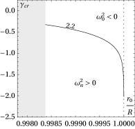
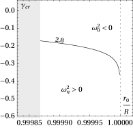
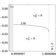
Figure 15: adiabatic index $\gamma_{\rm cr}$ as a function of the radius for four values of the electric charge, namely, $\frac{q^{2}}{R^{2}}=1.1$, $\frac{q^{2}}{R^{2}}=2.2$, $\frac{q^{2}}{R^{2}}=2.8$, and $\frac{q^{2}}{R^{2}}=2.99$, as indicated in the figure. Stability of regular tension black holes with positive enthalpy density. These regular black holes belong to region (e2), above the curve $C_{33}$ of Fig. 2 which is an enlargement of Fig. 2. The critical adiabatic index $\gamma_{\rm cr}$ for four values of the electric charge parameter $\frac{q^{2}}{R^{2}}=1.1$, $\frac{q^{2}}{R^{2}}=2.2$, $\frac{q^{2}}{R^{2}}=2.8$, and $\frac{q^{2}}{R^{2}}=2.99$, is shown as a function of the radius $\frac{r_{0}}{R}$. In each of the four plots, the line starts at a minimum radius $\frac{r_{0}}{R}$ on the curve $C_{33}$ for which $\gamma_{\rm cr}$ is negative and for larger $\frac{r_{0}}{R}$, $\gamma_{\rm cr}$ becomes more negative up to the line $\frac{r_{0}}{R}=1$. The light gray region on the left side of each plot corresponds to objects that are not regular tension black holes with positive enthalpy density configurations. The difference of this figure to Fig. 11, is that here the range of $\frac{r_{0}}{R}$ is widened in each plot.

we show the numerical results for the critical adiabatic index $\gamma_{\rm cr}$ as a function of the radius for four values of the electric charge, namely, $\frac{q^{2}}{R^{2}}=1.1$, $\frac{q^{2}}{R^{2}}=2.2$, $\frac{q^{2}}{R^{2}}=2.8$, and $\frac{q^{2}}{R^{2}}=2.99$, as indicated in the figure. The difference of this figure to Fig. 11, is that here in Fig. 15 the range of $\frac{r_{0}}{R}$ is widened in each plot to get a good portion of the plotted line, whereas in Fig. 11 the range of $\frac{r_{0}}{R}$ is fixed so that one sees clearly by a comparison between the four plots themselves the range of the validity of the solutions in the axis $\frac{r_{0}}{R}$.

References

- (1) B. S. Guilfoyle, “Interior Weyl-type solutions of the Einstein-Maxwell field equations”, Gen. Relativ. Gravit. 31, 1645 (1999); arXiv:gr-qc/9906089.
- (2) J. P. S. Lemos and V. T. Zanchin, “Electrically charged fluids with pressure in Newtonian gravitation and general relativity in spacetime dimensions: Theorems and results for Weyl type systems”, Phys. Rev. D 80, 024010 (2009); arXiv:0905.3553 [gr-qc].
- (3) J. P. S. Lemos and V. T. Zanchin, “Bonnor stars in spacetime dimensions”, Phys. Rev. D 77, 064003 (2008); arXiv:0802.0530 [gr-qc].
- (4) H. Andréasson, “Sharp bounds on the critical stability radius for relativistic charged spheres”, Commun. Math. Phys. 288, 715 (2009); arXiv:0804.1882 [gr-qc].
- (5) J. P. S. Lemos and V. T. Zanchin, “Sharp bounds on the radius of relativistic charged spheres: Guilfoyle’s stars saturate the Buchdahl-Andréasson bound”, Classical Quantum Gravity 32, 135009 (2015); arXiv:1505.03863 [gr-qc].
- (6) J. P. S. Lemos and E. J. Weinberg, “Quasiblack holes from extremal charged dust”, Phys. Rev. D 69, 104004 (2004); arXiv:gr-qc/0311051.
- (7) J. P. S. Lemos and V. T. Zanchin, “Gravitational magnetic monopoles and Majumdar-Papapetrou stars”, J. Math. Phys, 47, 042504 (2006); arXiv:gr-qc/0603101.
- (8) J. P. S. Lemos and O. B. Zaslavskii, “Quasiblack holes: Definition and general properties”, Phys. Rev. D 76, 084030 (2007); arXiv:0707.1094 [gr-qc].
- (9) J. P. S. Lemos and O. B. Zaslavskii, “Quasiblack holes with pressure: General exact results”, Phys. Rev. D 82, 024029 (2010); arXiv:1004.4651 [gr-qc].
- (10) J. P. S. Lemos and V. T. Zanchin, “Quasiblack holes with pressure: Relativistic charged spheres as the frozen stars”, Phys. Rev. D 81, 124016 (2010); arXiv:1004.3574 [gr-qc].
- (11) J. P. S. Lemos and O. B. Zaslavskii, “Compact objects in general relativity: From Buchdahl stars to quasiblack holes”, Int. J. Mod. Phys. D 29, 2041019 (2020); arXiv:2007.00665 [gr-qc].
- (12) J. P. S. Lemos and V. T. Zanchin, “Regular black holes: Guilfoyle’s electrically charged solutions with a perfect fluid phantom core”, Phys. Rev. D 93, 124012 (2016); arXiv:1603.07359 [gr-qc].
- (13) K. A. Bronnikov and J. C. Fabris, “Regular phantom black holes”, Phys. Rev. Lett. 96, 251101 (2006); arXiv:gr-qc/0511109.
- (14) O. B. Zaslavskii, “Regular black holes and energy conditions”, Phys. Lett. B 688, 278 (2010); arXiv:1004.2362 [gr-qc].
- (15) J. P. S. Lemos and V. T. Zanchin, “Regular black holes: Electrically charged solutions, Reissner-Nordström outside a de Sitter core”, Phys. Rev. D 83, 124005 (2011); arXiv:1104.4790 [gr-qc].
- (16) N. Uchikata, S. Yoshida, and T. Futamase, “New solutions of charged regular black holes and their stability”, Phys. Rev. D 86, 084025 (2012); arXiv:1209.3567 [gr-qc].
- (17) A. Flachi and J. P. S. Lemos, “Quasinormal modes of regular black holes”, Phys. Rev. D 87, 024034 (2013); arXiv:1211.6212 [gr-qc].
- (18) A. D. D. Masa, E. S. de Oliveira, and V. T. Zanchin, “Stability of regular black holes and other compact objects with a charged de Sitter core and a surface matter layer”, Phys. Rev. D 103, 104051 (2021); arXiv:2009.10948 [gr-qc].
- (19) J. P. S. Lemos and P. Luz, “All fundamental electrically charged thin shells in general relativity: From star shells to tension shell black holes, regular black holes, and beyond”, Phys. Rev. D 103, 104046 (2021); arXiv:2103.15832 [gr-qc].
- (20) J. P. S. Lemos and V. T. Zanchin, “Plethora of relativistic charged spheres: The full spectrum of Guilfoyle’s static, electrically charged spherical solutions”, Phys. Rev. D 95, 104040 (2017); arXiv:1704.07840 [gr-qc].
- (21) S. Chandrasekhar, “The dynamical instability of gaseous masses approaching the Schwarzschild limit in general relativity”, Astrophys. J. 140, 417 (1964).
- (22) R. Stettner, “On the stability of homogeneous, spherically symmetric, charged fluids in relativity”, Ann. Phys. 80, 212 (1973).
- (23) M. Omote and H. Sato, “A criterion for the stability of a charged sphere in general relativity”, Gen. Relativ. Gravit. 5, 387 (1974).
- (24) I. Glazer, “General relativistic pulsation equation for charged fluids”, Ann. Phys. 101, 594 (1976); Ann. Phys. 115, 498 (1978).
- (25) I. Glazer, “Stability analysis of the charged homogeneous model”, Astrophys. J. 230, 899 (1979).
- (26) F. de Felice, S. Liu, and Y. Yu, “Relativistic charged spheres: II. Regularity and stability”, Classical Quantum Gravity 16, 2669 (1999); arXiv:gr-qc/9905099.
- (27) P. Anninos and T. Rothman, “Instability of extremal relativistic charged spheres”, Phys. Rev. D 65, 024003 (2001); arXiv:gr-qc/0108082.
- (28) C. Posada and C. Chirenti, “On the radial stability of ultra-compact Schwarzschild stars beyond the Buchdahl limit”, Classical Quantum Gravity 36, 065004 (2019); arXiv:1811.09589 [gr-qc].
- (29) W. H. Press, S. A. Teukolsky, W. T. Vetterling, and B. P. Flannery, Numerical Recipes in Fortran 77: the Art of Scientific Computing (Cambridge University Press, Cambridge, 1992).
- (30) Q. Kong and A. Zettl, “Eigenvalues of regular Sturm-Liouville problems”, J. Differ. Equ. 131, 1 (1996).
- (31) M. Möller, “On the unboundedness below of the Sturm-Liouville operator”, Proc. Roy. Soc. Edinb. A 129, 1011 (1999).
- (32) A. Zettl, Sturm-Liouville Theory (American Mathematical Society, Providence, 2005).
- (33) H. M. Väeth and G. Chanmugam, “Radial oscillations of neutron stars and strange stars”, Astron. Astrophys. 260, 250 (1992).
- (34) D. Gondek, P. Haensel, and J. L. Zdunik, “Radial pulsations and stability of protoneutron stars”, Astron. Astrophys. 325, 217 (1997); arXiv:astro-ph/9705157.
- (35) S. E. El-gendi, “Chebyshev solution of differential, integral and integro-differential equations”, Comp. J. 12, 282 (1969).
- (36) J. P. Boyd, Chebyshev and Fourier spectral methods (Springer, Berlin 1989, second edition Dover 2013).
- (37) E. M. E. Elbarbary and M. El-Kady, “Chebyshev finite difference approximation for the boundary value problems”, Appl. Math. Comput. 139, 513 (2003).
- (38) A. H. S. Taher, A. Malek, and S. H. M. Masuleh, “Chebyshev differentiation matrices for efficient computation of the eigenvalues of fourth order Sturm-Liouville problems”, Appl. Math. Model. 37, 4634 (2013).
- (39) A. Jansen, “Overdamped modes in Schwarzschild-de Sitter and a Mathematica package for the numerical computation of quasinormal modes”, Eur. Phys. J. Plus 132, 546 (2017); arXiv:1709.09178 [gr-qc].