GW190521 as a dynamical capture of two nonspinning black holes

Abstract

Gravitational waves from $\sim 90$ black holes binary systems have currently been detected by the LIGO [1] and Virgo [2] experiments, and their progenitors’ properties inferred [3]. This allowed the scientific community to draw conclusions on the formation channels of black holes in binaries, informing population models and – at times – defying our understanding of black hole astrophysics. The most challenging event detected so far is the short duration gravitational-wave transient GW190521 [4, 5]. We analyze this signal under the hypothesis that it was generated by the merger of two nonspinning black holes on hyperbolic orbits. The best configuration matching the data corresponds to two black holes of source frame masses of $81^{+62}_{-25}M_{\odot}$ and $52^{+32}_{-32}M_{\odot}$ undergoing two encounters and then merging into an intermediate-mass black hole. We find that the hyperbolic merger hypothesis is favored with respect to a quasi-circular merger with precessing spins with Bayes’ factors larger than 4300 to 1, although this number will be reduced by the currently uncertain prior odds. Our results suggest that GW190521 might be the first gravitational-wave detection from the dynamical capture of two stellar-mass nonspinning black holes.

Theoretisch-Physikalisches Institut, Friedrich-Schiller-Universität Jena, Jena, 07743,Germany

Dipartimento di Fisica “Enrico Fermi”, Università di Pisa, Pisa, 56127, Italy

INFN sezione di Pisa, Pisa, 56127, Italy

Dipartimento di Fisica, Università di Torino, Torino, 10125, Italy

INFN sezione di Torino, Torino, 10125, Italy

Institut des Hautes Etudes Scientifiques, 35 Route de Chartres, Bures-sur-Yvette, 91440, France

Niels Bohr International Academy, Niels Bohr Institute, Blegdamsvej 17, 2100 Copenhagen, Denmark

1 Introduction

The gravitational-wave (GW) transient GW190521 is compatible with the quasi-circular merger of two heavy ($m_{1}\simeq 85M_{\odot}$, $m_{2}\simeq 66M_{\odot}$) black holes (BHs) resulting in an ${\simeq}150M_{\odot}$ intermediate-mass BH (IMBH) [4, 5]. The estimated BH component masses fall in a mass gap ${\simeq}65-120M_{\odot}$ for BHs formed directly from stellar collapse, and challenge standard scenarios on BHs formation[5, 6, 7, 8, 9, 10, 11, 12], suggesting the possibility of a progenitors formation through repeated mergers [13, 14]. The short duration ($\sim 0.1$ s) of GW190521 and the absence of a premerger signal, identified also by unmodeled (or weakly modeled) analyses[1], are critical aspects for the choice of waveform templates in matched filtering analyses and thus for the interpretation of the source. For example, under the hypothesis of a quasi-circular merger, matching the signal morphology requires fairly large in-plane components of the individual BH spins and results in a (weak) statistical evidence for orbital-plane precession. High orbital eccentricities are also compatible with the burst-like morphology of GW190521, but best-matching eccentric merger waveforms still require spin precession[15, 16]. Spin precessing binary black hole (BBH) mergers are known to be degenerate with head-on collisions[17]. However, a head-on BBH is disfavored with respect to a boson-star head on collision with a log Bayes’ factor of $-6.1$[18]. Other proposed interpretations involve a high-mass black hole-disk system [19] or an intermediate mass ratio inspiral[20] (see also[21]), and indicate that the origin of GW190521 is still unsettled.

In this Letter we analyse GW190521 within the scenario of a binary black hole (BBH) dynamical capture and compare this hypothesis to that of a quasi-circular merger. Dynamical captures have a phenomenology radically different from quasi-circular mergers[22, 23, 24]. The close passage and capture of the two objects in hyperbolic orbits naturally accounts for the short-duration, burst-like waveform morphology of GW190521 even in the absence of spins. Moreover, possibile explanations of the high component masses rely on second-generation BHs, stellar mergers in young star clusters and BH mergers in active galactic nuclei disks[6, 25, 26, 7, 8, 9, 10, 11, 12], for which dynamical captures are possible. While no observational evidence for GWs from dynamical captures existed prior to our work, such events are not incompatible with the current detection rates [27, 28], although these rates would require corrections to take into account the large masses of GW190521[29].

2 Phenomenology of hyperbolic mergers

A significant progress in constructing waveform templates for black hole binaries on hyperbolic orbits has been recently made within the effective-one-body (EOB) approach[30, 31]. The EOB method[32] is a powerful analytical formalism that suitably resums post-Newtonian (PN) results[33, 34] (obtained via a perturbative expansion of Einstein’s field equations in powers of $v/c$, with $v$ the typical speed of the system) in the weak-field, small-velocity regime and makes them reliable and predictive also when the field is strong and velocities are comparable to $c$, i.e. up to merger and ringdown. This framework can be extended to fully account for the dynamical capture phenomenology, and delivers complete waveform templates from hyperbolic mergers[30, 31]. The method is a generalization of the quasi-circular, spin-aligned waveform model TEOBResumS[35] to deal with arbitrarily eccentric orbits, from eccentric inspirals to hyperbolic mergers. For simplicity, however, the EOB analytical waveform for hyperbolic mergers does not contain next-to-quasi-circular corrections informed by numerical relativity (NR) simulations and it is completed by a NR-informed quasi-circular ringdown[35]. The reason for this choice is that, although some NR simulations are available[36, 37, 38, 22, 23, 39, 40], a systematic coverage of the BBH parameter space for hyperbolic orbits is currently missing.

Although the model can be extended to include aligned spins and subdominant multipoles in the waveforms, here we focus on nonspinning BBHs and use only the dominant $\ell=m=2$ quadrupole mode, which has been more extensively tested , and was shown to be more than 97$\%$ faithful to NR (see Methods). The inclusion of spins is expected to modify the most likely values of the parameters correlated with the spins, such as the mass ratio, but not e.g. the total mass of the binary. The evidence of the analysis, too, is expected to vary due to the different prior volume explored. However, since the nonspinning model is contained within the spinning one, point estimates such as the maximum likelihood should not decrease with the addition of spin interactions.

The EOB relative motion is described using mass-reduced phase-space variables $(r,\varphi,p_{\varphi},p_{r_{*}})$, related to the physical ones by [in geometric units $G=c=1$] $r=R/M$ (relative separation), $\varphi$ (orbital phase), $p_{r_{*}}\equiv P_{R_{*}}/\mu$ (radial momentum), $p_{\varphi}\equiv P_{\varphi}/(\mu M)$ (angular momentum) and $t\equiv T/M$ (time), where $\mu\equiv m_{1}m_{2}/M$ and $M\equiv m_{1}+m_{2}$. The EOB Hamiltonian is $\hat{H}\equiv H/\mu\equiv\nu^{-1}\sqrt{1+2\nu(\hat{H}_{\rm eff}-1)}$, with $\nu\equiv\mu/M$ and $\hat{H}_{\rm eff}$ is the effective Hamiltonian[35, 30, 31]. For nonspinning binaries, the configuration space can be characterized by the mass ratio $q=m_{1}/m_{2}\geq 1$, the initial energy $E_{0}/M$ and the initial reduced orbital angular momentum ${p_{\varphi}^{0}}$ [31]. Similarly to the motion of a test particle moving around a Schwarzschild BH, the EOB behavior of a hyperbolic encounter is characterized by the EOB potential energy $E_{\rm EOB}\equiv M\sqrt{1+2\nu(\hat{W}_{\rm eff}-1)}$, where $\hat{W}_{\rm eff}=\sqrt{A(r)(1+p_{\varphi}^{2}/r^{2})}$ is the effective potential energy. Here, $A(r)\equiv P^{1}_{5}[A_{\rm 5PN}(r)]$ is the Padé resummed EOB radial potential, where $A_{\rm 5PN}(r)=1-2/r+\nu a(\nu,r)$ indicates its Taylor-expanded form, that reduces to the Schwarzschild case in the test-particle limit, $\nu=0$. The function $a(\nu,r)$ incorporates high-order corrections up to 5PN and it is additionally informed by NR simulations[35, 30]. The solution $\partial_{r}W_{\rm eff}=\partial_{r}^{2}W_{\rm eff}=0$ defines last stable orbit (LSO) parameters $(r_{\rm LSO},p_{\varphi}^{\rm LSO})$. When $p_{\varphi}>p_{\varphi}^{\rm LSO}$, $W_{\rm eff}$ has both a maximum and a minimum and, depending on $E_{0}/M$, bound as well as unbound configurations are present. In the absence of radiation reaction, unbound configurations are defined by the condition $E_{0}/M>1$. We define $E_{\rm min}/M\equiv\nu\hat{H}(r_{0},q,p_{\varphi},p_{r}=0)$ the energy corresponding to the initial separation and $E_{\rm max}/M=\max_{r}\left[\nu\hat{H}(r,q,p_{\varphi},p_{r}=0)\right]$. For a given $p_{\varphi}$, the values $(E_{\rm max},E_{\rm min})$ correspond respectively to unstable and stable circular orbits, analogously to Schwarzschild geodesics. When $E_{0}>E_{\rm max}$ the objects fall directly onto each other without forming metastable configurations (e.g., for head-on collisions, corresponding to $p_{\varphi}=0$). When $1<E_{0}/M\leq E_{\rm max}/M$, the phenomenology changes from direct plunge, to on up to many close passages before merger, to zoom-whirl behavior or even scattering[36, 38, 39].

In the presence of radiation reaction, the qualitative picture remains unchanged (as also observed in NR simulations[23]), although the threshold between the two qualitative behaviors is not simply set by $E_{\rm max}$, but it is also affected by GW losses. The latter are taken into account through the azimuthal and radial radiation reaction forces $({\cal F}_{\varphi},{\cal F}_{r})$ described in detail in[30, 31]. The dynamics of each configuration can be characterized by counting the number of peaks of the orbital frequency $\Omega(t)\equiv\dot{\varphi}$, each peak corresponding to a periastron passage[31]. Figure 1 illustrates the $(E_{0}/M,{p_{\varphi}^{0}})$ parameter space, defined using the peaks of $\Omega(t)$, of a nonspinning binary with $q=1.27$, corresponding to the best-matching mass ratio for the GW190521 analysis. The different colors indicate the number of encounters. Although the two dark blue areas, above and below the magenta zone, possess a single peak in $\Omega$, they correspond to different phenomenologies. The dark-blue region above the magenta area corresponds to a direct capture scenario, that eventually leads to a ringdown phase. The dark-blue region below the magenta area corresponds to a scattering scenario. The single-burst waveform morphology is obtained for $(E_{0}/M,{p_{\varphi}^{0}})$ within the blue capture region as well as the upper boundary of the magenta region, until a distinct second burst of GWs does not appear before the one corresponding to the final merger. The single burst phenomenology also occurs in the white region $E_{0}>E_{\rm max}$ in Fig. 1, where there exist systems with low values of ${p_{\varphi}^{0}}$ and large initial energies. Waveforms emitted by such binaries are dominated by the ringdown.

3 Results

We analyze GW190521 under the hypothesis that it was generated by a dynamical capture of two nonspinning BHs. We use two different priors for the initial energy of the binary: an “unconstrained” prior (UE₀) and a “constrained” prior CE₀ (see Methods). The results of the analysis corresponding to the UE₀ and CE₀ priors are summarized in the second and third columns of Table 1 respectively. The consistency of the two measurements confirms the robustness of our modeling choices. Focusing on global fitting quantities we find, respectively for the UE₀ (CE₀) priors, maximum likelihood values $\log({\cal L})_{\rm max}=123.2\,(123.0)$, and Bayesian evidences $\log{\cal B}^{\rm signal}_{\rm noise}=84.0\pm 0.18\,(83.3\pm 0.18)$, while the recovered matched-filter signal-to-noise ratio (SNR) is equal to 15.2 (15.4). Employing the standard cosmology [41], we find component masses in the source frame $(m_{1},m_{2})=(85^{+88}_{-22},59^{+18}_{-37})M_{\odot}$ for the UE₀ case and $(m_{1},m_{2})=(81^{+62}_{-25},52^{+32}_{-32})M_{\odot}$ in the CE₀ case. Figure 2 illustrates the $(E_{0},{p_{\varphi}^{0}})$ parameter space selected by the analysis, with colors highlighting configurations with different number of encounters $N$. The figure shows that, despite GW190521 consisting of a single GW burst around the analyzed time, many of the configurations selected, and in particular the most probable ones, correspond to two encounters.

The phenomenology corresponding to the set of maximum likelihood parameters selected by the analysis are shown in Fig. 3. The EOB relative trajectory (top panel) is complemented by the corresponding waveform templates projected onto the three detectors and compared to the whitened LIGO-Virgo data around the time of GW190521. Thicker lines highlight the last part of the dynamics, which exactly covers the portion of the signal displayed in the bottom panel. The magnitude of the first GW burst predicted by the EOB analysis (not shown in the plot) is comparable to the detector noise and would occur outside the analysis window. However, we find that such first burst is not a robust feature across samples, occurring at different times and smaller amplitudes for different points and not occuring at all for others (see Fig. 2). Given this consideration and the small amplitude of such first burst, we do not expect an extension of the analysis segment to impact our main conclusions.

In order to compare the hyperbolic capture with the quasi-circular merger hypothesis, we perform a new quasi-circular analysis with the precessing surrogate model NRSur7dq4[42] and with the quasi-circular precessing flavor of TEOBResumS, TEOBResumSP [43, 44]. To minimize systematic effects, we consistently use the bajes pipeline[45] with the same settings discussed above for all the runs. The prior distributions for the mass parameters and the extrinsic parameters are also identical to the ones used in the hyperbolic capture analysis with TEOBResumS, while the prior on the spin components is chosen to be uniform in the spin magnitudes and isotropic in the angles[4]. When including higher modes we disable phase marginalization.

In Table 1 we quote maximum likelihood and matched-filter SNR values obtained from the full unmarginalised posterior. The quasi-circular precessing analyses with bajes and NRSur7dq4 are in agreement with those obtained by LVK[4], confirming the reliability of the infrastructure adopted for the inference. The maximum SNR recovered via our pipeline is lower by $0.7$ than the one extracted from the public LVK samples. We attribute this discrepancy to differences in data-processing between pipelines, small differences in the prior boundaries and the sampling itself. The use of consistent settings in our new runs with the model used by the LVK excludes that such discrepancies affect the comparison against the non-circular analysis.

The TEOBResumSP analyses display consistency with the NR surrogate. When PE is performed with the dominant $(2,2)$ mode, it yields $\log\mathcal{L}_{\rm max}=106.0$, $\rm{SNR}_{\rm max}=14.7$ and $\log\mathcal{B}^{\rm signal}_{\rm noise}=72.95\pm 0.08$. This indicates that the observed increases in these statistics when employing the dynamical capture model are not driven by subtle differences between waveform families (EOB and NR surrogate).

4 Discussion

Despite the different hypotheses on the coalescence process, our results on the component masses are in good agreement with the ones obtained from a quasi-circular model. This confirms that an IMBH is formed at the end of the coalescence also in the hyperbolic merger scenario. The consistency on the total mass is not surprising, given that the dominant contribution to this parameter comes from the determination of the ringdown frequency [4]. However, the dynamical capture model is able to fit GW data better than the quasi-circular scenario despite having four less degrees of freedom, with a 16 e-fold increase in the maximum likelihood value. For comparison, the distribution of $\log\mathcal{L}$ of the quasi-circular analysis spans a $\sim 26$ e-folds range and has median $\sim 9$ e-folds smaller than its maximum value. If we assume this difference to be representative of the statistical uncertainty $\sigma$ on the likelihood, we find that our result lies about $3\sigma$ from the median of the quasi-circular analysis and $2\sigma$ from its maximum value. Under the dynamical capture assumption, we obtain a matched-filter SNR $\rho=15.4$, larger by almost a unity with respect to the same value obtained using quasi-circular waveforms. Similarly to the $\log\mathcal{L}$, the maximum SNR of the hyperbolic analysis lies about $1\sigma$ from the corresponding value of the quasi-circular analysis and $2\sigma$ from its median.

The fit improvement registered by these two indicators is confirmed by the Bayesian evidences, keeping into account the full correlation structure of the parameter space, which imply odds ${\gtrsim}4315{:}1$ in favor of the dynamical encounter scenario against the quasi-circular scenario. This number is expected to be an optimistic estimate of the posterior odds, due to the prior odds disfavouring a dynamical capture scenario compared to a quasi-circular binary. However, estimates of prior odds are currently not reliable due to orders of magnitudes uncertainties on dynamical capture rates in this mass range [29] and, as such, we do not attempt to quantify them directly. Given our (conservative) Bayes factor, we estimate that the capture interpretation is favored with respect to a quasi-circular stellar-collapse scenario[6] so long as the rates of such events is larger than $5\times 10^{-3}\rm{Gpc}^{-3}\rm{yr}^{-1}$. This number is computed by imposing that the posterior odds are lager than one, i.e. that $4315\times R^{\rm dc}/R^{\rm qc}>1$, where $R^{\rm dc}$ is the rate of dynamical capture events and $R^{\rm qc}=23.9$ Gpc^-3 yr^-1 as estimated by LVK[6]. Notably, the Bayes’ factors receive a penalty disfavouring the quasi-circular hypothesis due to the larger dimensionality of this model which is not phase marginalized and includes precessing spins degrees of freedom, although the latter are only weakly measurable. Additionally, some railing against the prior can be observed for the $E_{0}/M$ and the UE₀ $p_{\varphi}^{0}$ posterior samples, which might affect the estimation of the dynamical capture evidence. However, the choice of prior bounds in this analysis was dictated either by physical boundaries, and hence cannot be relaxed, or by considerations on computational cost and model validity in a region – that of head-on mergers – which was shown to have little support for the phenomenology observed[18]. In light of the above caveats, the Bayesian evidences alone represent useful, but not decisive proof in favor of the capture scenario.

Nonetheless, these two results combined constitute data-driven indicators that the interpretation of GW190521 within the dynamical capture scenario seems preferred over a quasi-circular spin-precessing merger[1, 21]. No other analysis shows such large improvements in evidence and log-likelihood with respect to the equal-mass, quasi-circular scenario[15, 16, 18]. At the same time, the absolute values of evidence and maximum likelihood estimated in some studies[21] are almost as large as those obtained in this work. These values were however obtained with a model which is less NR-faithful in the quasi-circular case than the NRSur7dq4 model considered in this work. Although a direct comparison is not possible given the different PE infrastructure, sampler, models and priors explored, this fact highlights the necessity of exploring multiple hypothesis and model selection to understand such short GW transients. Our findings are consistent with the fact that burst-like waveforms from highly eccentric or head-on BBH collision may be confused with mildly precessing quasi-circular binaries[17] and viceversa. In the supplementary material we confirm this degeneracy to a certain extent, but we show that the preference we obtain for the non-circular model is incompatible with the true signal being a quasi-circular merger embedded in gaussian noise. Regarding other possible scenarios, a quantitative comparison is currently not possible since they have not been analyzed with full Bayesian studies and/or complete waveform templates[18, 15, 19].

While our analysis selects a two-encounters merger as best-fitting capture scenario (Fig. 3), the orbital dynamics of these encounters is rather sensitive to changes in both the conservative and nonconservative part of the dynamics[31], as also evident from Fig. 11 of[31]. Going beyond the conservative assumptions behind our analysis, future work will explore the impact of spin and of higher waveform multipoles, as well as consider systematic comparisons between our (improved[46]) EOB model and a larger number of NR simulations. The inclusion of additional, physically motivated, degrees of freedom (e.g., BH spins) is expected to further shed light on the nature of GW190521.

5 Methods

5.1 Waveform model validation

The EOB analytical model employed in this analysis, TEOBResumS [30, 31] , generates waveforms and scattering angles that are faithful to NR simulations of nonspinning BBH along eccentric and scattering orbits[39, 30, 31]. The model is directly validated in the regime of interest by comparisons against new NR data targeted at GW190521. The simulations parameters are chosen to be compatible with the ones obtained by our hyperbolic analysis. Additionally, we compare against 46 selected nonspinning, highly eccentric NR simulations[47], to validate the model in a similar regime. Crucially, for all configurations considered, the quasi-circular ringdown provides a reliable approximation of the final stage of the coalescence, and the model is more than $97\%$ faithful to NR. This is not surprising, and can be attributed to the circularization of the system during the last phases of the coalescence. Such results ensure the reliability of our model in extracting astrophysical properties from GW signals. Head-on collisions, conversely, are not well approximated by our model. Finally, reliability of this EOB approach in describing dynamical captures is further verified in the test-mass limit of a body captured by a Schwarzschild BH, using the waveforms computed numerically using black hole perturbation theory[48, 49]. These results are summarized in the Supplementary Material; further details and more in-depth comparisons will also be presented in a future work (Andrade et. al., in preparation).

5.2 GW190521 analysis

The publicly released GW190521 data are analyzed around time $t_{\rm GPS}=1242442968$, with an $8\,$s time-window and in the range of frequencies $[11,512]\,$Hz using the bajes pipeline [45]. We employ the power-spectral-density estimate and calibration envelopes publicly available from the GW Open Science Center [50]. The Bayesian analysis uses the dynesty sampler [51] with 2048 live points. We use a uniform prior in the mass components $(m_{1},m_{2})$ exploring the ranges of chirp mass $\mathcal{M}_{c}\in[30,200]\,M_{\odot}$ and mass ratio $q\in[1,8]$. The luminosity distance is sampled assuming a volumetric prior in the range $[1,10]\,$Gpc. We analytically marginalize over the coalescence phase, and sample the coalescence time in $t_{s}\in[-2,2]\,$s with respect to the central GPS time.

The key quantities to sample the configuration space of hyperbolic mergers are $(E_{0}/M,{p_{\varphi}^{0}})$. The initial angular momentum is uniformly sampled within ${p_{\varphi}^{0}}\in[3.5,5]$, and further imposing ${p_{\varphi}^{0}}\geq p_{\varphi}^{\rm LSO}$ for any $q$. The initial energy is uniformly sampled in the interval $E_{0}/M\in[1.0002,1.025]$ but with two different additional constraints that result in two different prior choices: (${\rm UE_{0}}$) Unconstrained prior: $E_{0}\geq E_{\rm min}$; (${\rm CE_{0}}$) Constrained prior: $E_{\rm min}\leq E_{0}\leq E_{\rm max}$. The ${\rm UE_{0}}$ prior spans a larger portion of the parameter space, notably including direct capture, although the dynamic remains far from the head-on collision case. The ${\rm CE_{0}}$ prior is contained in the first, and restricts the parameter space to systems closer to stable configurations, for which the orbital dynamics substantially contributes to the waveform and the ringdown description is expected to be more accurate.

Data Availability Data is available onn Zenodo, with DOI 10.5281/zenodo.7081337.

Code Availability The eccentric waveform model used in this work, TEOBResumS, is publicly available at: https://bitbucket.org/eob_ihes/teobresums/ and results presented in this paper have been obtained with the version tagged ${\tt eccentric.v0\_a6c\_c3\_circularized}$. Similarly, TEOBResumSP is publicly availabe at the same address, and results presented here have been obtained with the version having git hash ${\tt 56f20ad}$.

Acknowledgments We are grateful to T. Damour, J. A. Font and T. Andrade for discussions. We are also grateful to D. Chiaramello for collaboration at the beginning of the project. We also thank B. Daszuta, F. Zappa, W. Cook and D. Radice for supporting the development of the GR-Athena++ code and for help with the NR simulations presented in the Supplementary Material. R.G. acknowledges support from the Deutsche Forschungsgemeinschaft (DFG) under Grant No. 406116891 within the Research Training Group RTG 2522/1. M.B., S.B. acknowledge support by the EU H2020 under ERC Starting Grant, no. BinGraSp-714626. M.B. acknowledges partial support from the Deutsche Forschungsgemeinschaft (DFG) under Grant No. 406116891 within the Research Training Group RTG 2522/1. G.C. acknowledges support by the Della Riccia Foundation under an Early Career Scientist Fellowship, and funding from the European Union’s Horizon 2020 research and innovation program under the Marie Sklodowska-Curie grant agreement No. 847523 ‘INTERACTIONS’, from the Villum Investigator program supported by VILLUM FONDEN (grant no. 37766) and the DNRF Chair, by the Danish Research Foundation. Computations were performed on the national HPE Apollo Hawk at the High Performance Computing Center Stuttgart (HLRS), on the ARA cluster at Friedrich Schiller University Jena and on the Tullio sever at INFN Turin. The ARA cluster is funded in part by DFG grants INST 275/334-1 FUGG and INST275/363-1 FUGG and by the ERC Starting Grant, grant agreement no. BinGraSp-714626. The authors acknowledge HLRS for funding this project by providing access to the supercomputer HPE Apollo Hawk under the grant number INTRHYGUE/44215. We thank E. Ferrari for speed-up coding work on Tullio.
This research has made use of data, software and/or web tools obtained from the Gravitational Wave Open Science Center (https://www.gw-openscience.org), a service of LIGO Laboratory, the LIGO Scientific Collaboration and the Virgo Collaboration. LIGO is funded by the U.S. National Science Foundation. Virgo is funded by the French Centre National de Recherche Scientifique (CNRS), the Italian Istituto Nazionale della Fisica Nucleare (INFN) and the Dutch Nikhef, with contributions by Polish and Hungarian institutes.

Author contributions S.B and A.N. contributed to the origination of the idea. A.N., P.R., R.G., and S.B. developed and tested the waveform model. R.G., M.B., and G.C. performed the analyses and S.A. carried out Numerical Relativity simulations. R.G. produced all the figures. All authors worked out collaboratively the general details of the project. All authors helped edit the manuscript.

Competing interests The authors declare no competing interests.

Reference	This paper					LVK[4]	Gayathri et al.[15]	Romero-Shaw et al.[16]
Waveform	TEOBResumS[30, 31]	TEOBResumS[30, 31]	TEOBResumSP[44]	NRSur7dq4[42]	NRSur7dq4[42]	NRSur7dq4[42]	NR[47]	SEOBNRE[52]
$E_{0}$ prior	Unconstrained (${\rm UE_{0}}$)	Constrained (${\rm CE_{0}}$)	–	–	–	–	–
Multipoles	$(\ell,|m|)=(2,2)$	$(\ell,|m|)=(2,2)$	$(\ell,|m|)=(2,2)$	$(\ell,|m|)=(2,2)$	$\ell\leq 4$	$\ell\leq 4$	–	–
$m_{1}$ [$M_{\odot}$]	$85^{+88}_{-22}$	$81^{+62}_{-25}$	$90^{+19}_{-14}$	$102^{+35}_{-23}$	$84^{+17}_{-12}$	$85^{+21}_{-14}$	$102^{+7}_{-11}$	$92_{-16}^{+26}$
$m_{2}$ [$M_{\odot}$]	$59^{+18}_{-37}$	$52^{+32}_{-32}$	$66^{+10}_{-8}$	$64^{+19}_{-25}$	$71^{+16}_{-18}$	$66^{+17}_{-18}$	$102^{+7}_{-11}$	$69_{-19}^{+18}$
$M_{\rm source}$ [$M_{\odot}$]	$151^{+73}_{-51}$	$130^{+75}_{-43}$	$156^{+25}_{-15}$	$164^{+40}_{-23}$	$153^{+29}_{-19}$	$150^{+29}_{-17}$	–	–
$m_{2}/m_{1}\leq 1$	$0.69^{+0.27}_{-0.52}$	$0.63^{+0.31}_{-0.43}$	$0.73^{+0.21}_{-0.15}$	$0.62^{+0.32}_{-0.30}$	$0.86^{+0.12}_{-0.30}$	$0.79^{+0.19}_{-0.29}$	–	–
$\chi_{\rm eff}$	–	–	$-0.05^{+0.09}_{-0.12}$	$0.01^{+0.24}_{-0.26}$	$-0.03^{+0.25}_{-0.26}$	$0.08^{+0.27}_{-0.36}$	$0$	$0.0_{-0.2}^{+0.2}$
$\chi_{\rm p}$	–	–	$0.72^{+0.16}_{-0.22}$	$0.71^{+0.22}_{-0.36}$	$0.79^{+0.16}_{-0.40}$	$0.68^{+0.25}_{-0.37}$	0.7	–
$e$	–	–	–	–	–	–	$0.67$	$0.11$
$E^{0}/M$	$1.014^{+0.009}_{-0.012}$	$1.014^{+0.010}_{-0.012}$	–	–	–	–	–	–
${p_{\varphi}^{0}}$	$4.18^{+0.50}_{-0.62}$	$4.24^{+0.57}_{-0.37}$	–	–	–	–	–	–
$D_{L}$ [Gpc]	$4.7^{+4.8}_{-2.7}$	$6.1^{+3.3}_{-3.7}$	$4.5^{+1.2}_{-1.2}$	$3.9^{+2.3}_{-1.9}$	$4.8^{+2.3}_{-2.2}$	$5.3^{+2.4}_{-2.6}$	$1.84^{+1.07}_{-0.054}$	$4.1^{+1.8}_{-1.8}$
SNRmax	$15.2$	$15.4$	$14.7$	$14.7$	$14.6$	$15.4$	–	–
$\log({\cal L})_{\rm max}$	$123.2$	$123.0$	$106.0$	$107.0$	$105.6$	–	–	–
$\log{\cal B}^{\rm signal}_{\rm noise}$	$84.00\pm 0.18$	$83.30\pm 0.18$	$72.95\pm 0.08$	$74.76\pm 0.11$	$74.86\pm 0.11$	–	–	–

Table 1: Source parameters of GW190521. We indicate the mass of the heavier (lighter) object with $m_{1}$ ($m_{2}$), $M_{\rm source}$ is the total mass in the frame of the source, $\chi_{\rm eff}$ is the effective spin along the orbital angular momentum, while $\chi_{\rm p}$ is the effective precessing spin[4]. The second and third columns report our new results, obtained with the hyperbolic capture model[31] with the two different prior choices on the energy. The fourth, fifth and sixth columns report the results obtained in this work with the quasi-circular models TEOBResumSP and NRSur7dq4. For reference, the remaining columns report results of other analyses[4, 15, 16]. We employ the standard cosmology of Planck[41] to compute source frame masses. Median values and $90\%$ credible intervals are quoted and natural logarithms are reported. The SNR values correspond to the matched-filter estimates.

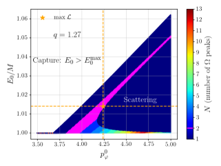
Figure 1: Number of encounters as a function of the initial energy and angular momentum. Parameter space for nonspinning hyperbolic encounters predicted using the TEOBResumS EOB model and fixing $q\equiv m_{1}/m_{2}=1.27$. Here $({p_{\varphi}^{0}},E_{0})$ are the EOB initial angular momentum and energy, while $E_{\rm max}^{0}$ is the value corresponding to unstable circular orbit. For $E_{0}<E_{0}^{\rm max}$, each color labels the number of peaks (i.e. of periastron passages) $N$ of the EOB orbital frequency $\Omega$. The orange star labels the maximum likelihood values $(\bar{p}_{\varphi}^{0},\bar{E}_{0})$ corresponding to the constrained analysis, see Table 1.

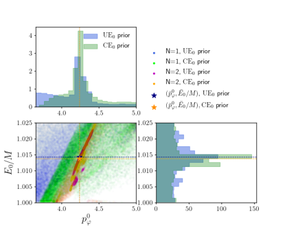
Figure 2: Energy-momentum marginalized two dimensional posterior. Marginalized two-dimensional posterior distributions of the initial energy $E_{0}$ and initial angular momentum ${p_{\varphi}^{0}}$ for the constrained (${\rm CE_{0}}$) and unconstrained (${\rm UE_{0}}$) energy prior choices. The colors highlight the different waveform phenomenologies, with $N=1$ (blue and green) or $N=2$ (magenta and orange) peaks in the orbital frequency. The maximum likelihood values $(\bar{p}_{\varphi}^{0},\bar{E}_{0})$ are highlighted with red (${\rm UE_{0}}$ prior) and dark-orange (${\rm CE_{0}}$ prior) stars.

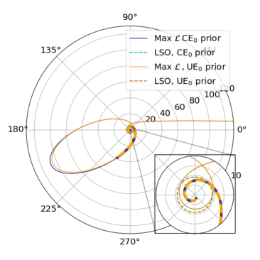
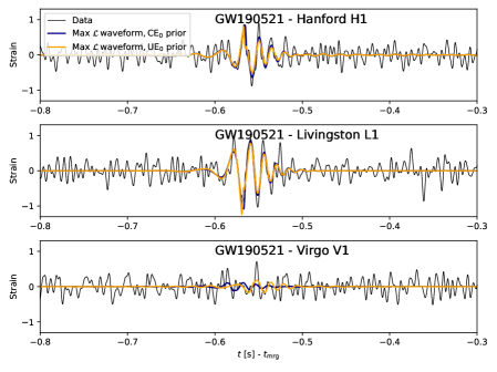
Figure 3: Maximum likelihood configurations with the two different energy priors, ${\rm UE_{0}}$ (orange) and ${\rm CE_{0}}$ (blue). Top: the $(r,\varphi)$ EOB relative orbit. Bottom: the waveform templates projected onto the three detectors compared to the whitened LIGO-Virgo data around the time of GW190521. The most probable last stable orbits (LSO) are highlighted with gold (${\rm UE_{0}}$ prior) and cyan (${\rm CE_{0}}$ prior) dashed lines and are located, respectively, at $\bar{r}_{\rm LSO}=4.54$ and $\bar{r}_{\rm LSO}=4.52$. Corresponding mass ratios are $\bar{q}=1.04$ and $\bar{q}=1.27$. The inset highlights the first close encounter, that is then followed by a highly eccentric orbit that eventually ends up with a plunge and merger phase. The part of the trajectory from $\sim(t_{\rm GPS}-0.8$ s$)$ to merger, which contributes to the second GW burst, is highlighted with thicker lines in the plot. Note that the GW bursts corresponding to the first encounter occur ${\sim}4$ s before the GW190521 time, their magnitude is comparable to the detector noise and are outside the segment of data analyzed.

Supplemental Material

5.3 Validation of the dynamical capture model

The EOB[32]^,Buonanno:2000ef,Damour:2000we,Damour:2001tu,Damour:2015isa waveform model TEOBResumS employed in our study is based on an highly accurate approximant for quasi-circular binaries Nagar:2018zoe, Nagar:2019wds, Nagar:2020pcj, Riemenschneider:2021ppj. The eccentric model has been extensively tested in previous works[30, 49] via mismatch and waveform phasing comparisons. In detail, the model has been compared to:

1. 28 equal-mass mildly eccentric NR simulations[30] from the Simulating eXtreme Spacetimes (SXS) collaborationChu:2009md,Lovelace:2010ne,Lovelace:2011nu,Buchman:2012dw, Hemberger:2013hsa, Scheel:2014ina,Blackman:2015pia, Lovelace:2014twa,Mroue:2013xna,Kumar:2015tha,Chu:2015kft, Boyle:2019kee,SXS:catalog. The comparison involved either time-domain phasing analysis or EOB/NR unfaithfulness computations. For completeness, this second analysis is repeated here with the implementation of the model employed in the analysis, and illustrated in Fig. 1. The model shows robust mismatches well below the $3\%$ threshold for system with masses ranging from $20M_{\odot}$ to $200M_{\odot}$ with the Advanced LIGO design sensitivity curveaLIGODesign_PSD.

2. 10 equal-mass scattering simulations from[39] used to check the scattering angle, but for which waveforms are not available[31].

3. 111 waveforms generated by a nonspinning test particle along planar geodesics in Kerr spacetime with eccentricities up to 0.9 and dimensionless Kerr spin magnitude up to $\hat{a}=0.9$. The analysis was also extended to nongeodesic motion considering the transition from inspiral to plunge driven by the EOB radiation reaction force considered in this work. Dynamical capture scenarios on a Schwarzschild spacetime were also considered. The accuracy of the fluxes has been studied in Sec. IV of Albanesi et al.[49], while the waveform has been analyzed in Sec. V. In particular, the analytical/numerical comparisons for the non-geodesics configurations can be found in Fig. 13 and Fig. 14 therein.

These tests demonstrate the goodness of our model in a regime which is, in principle, different from the one explored here, where an almost equal-mass system undergoes a dynamical capture. Notably, however, some important insight can be extrapolated from this information. Firstly, we observe that although the use of a circular ringdown is an approximation, the tests against test-mass waveforms from dynamical encounters show a good performance for the configurations that circularize during the last encounter, i.e. those selected by the parameter estimation, see in particular Fig. 14 of[49]. The region where the circular ringdown performs less well is the direct-capture and head-on scenario (also expected on physical grounds). However, these configurations are also excluded from the parameter estimation by their smaller likelihood values. Secondly, the comparison with eccentric comparable mass data proves that the radiation reaction employed is highly accurate in that regime. Finally, the EOB/NR comparisons of the scattering angle of relativistic equal-mass BBH is a strong test of the dynamics (of both the conservative and dissipative sector), that probes the model in a very challenging physical scenario[31].

To further corroborate these observations in the regime of direct interest for this publication, we produced six equal-mass, nonspinning simulations of highly eccentric systems or dynamical captures using the NR code ${\tt GR-Athena++}$ Daszuta:2021ecf, see Table 1. Three simulations reproduce configurations of Gold and Bruegmann [23] ($\tt{gb42\_N256}$, $\tt{gb48\_N256}$ and $\tt{gb50\_N256}$); the three remaining ones are instead completely new configurations ($\tt{Hq1\_a5}$, $\tt{Hq1\_b5}$ and $\tt{Hq1\_c5}$) with initial conditions chosen to target the parameter space selected by our GW190521 analysis. In order to compare NR and EOB waveforms, one needs consistent initial energy, angular momentum and separation. While the first two quantities are in principle gauge-invariant, to get the latter we need to convert from Arnowitt-Deser-Misner (ADM) coordinates to EOB coordinates using a 2PN-accurate transformation [32]Bini:2012ji. However, the existence of NR junk radiation, resolution effects as well as the finite PN order of the ADM to EOB transformation can cause small differences between the NR and EOB initial data. While small variations in the energy and angular can significantly change the phenomenology of the waveform, as shown in Fig. 2 of[31], small inaccuracies in the initial separation are not relevant as long as the bodies are initially far enough. In this scenario, the effect of the radiation reaction is negligible at the beginning of the evolution, and small shifts in initial separation correspond to global constant time shifts. As such, in order to estimate the “optimal” values of $(\hat{E}_{0},\hat{p}_{\varphi}^{0})$, we first additionally minimized the mismatch on the initial energy and angular momentum over a small interval around the values extracted from the procedure described above, allowing a relative error up to $1\%$ in energy and up to $6\%$ in angular momentum. This procedure was performed only for a single reference value of total mass ($M=250M_{\odot}$, i.e. the detector frame mass of GW190521), using the expression:

$$\bar{\mathcal{F}}=1-\max_{t_{0},\phi_{0},\hat{E}_{0},\hat{p}_{\varphi}^{0}}\frac{(h^{\rm NR},h^{\rm EOB})}{\sqrt{(h^{\rm NR},h^{\rm NR})(h^{\rm EOB},h^{\rm EOB})}}\,,$$ (S1)

where $(\cdot,\cdot)$ denotes the usual noise weighted inner product

$$(a,b)=4\Re\int_{f_{0}}^{f_{max}}\frac{\tilde{a}(f)\tilde{b}(f)}{S_{n}(f)}df\,,$$

and $S_{n}$ is the power spectral density (PSD) of the detector, in this case chosen to be GW190521 Hanford’s PSD. The initial conditions found with this procedure are then employed to compute $\bar{\mathcal{F}}$ for all values of the total mass $M$ considered using the standard definition of mismatch (the same as above, without varying the initial energy and angular momentum). We considered frequencies between $11$ and $512$ Hz and total masses $M\in[100,300]M_{\odot}$. We found mismatches between $0.2\%$ and $3\%$. Details about the simulations are listed in Table 1, while the results of the computation can be seen in Fig. 2. The corresponding time-domain EOB/NR phase comparisons of the $\ell=m=2$ waveform are shown in Fig. 3. Let us recall that we use the following multipolar decomposition of the strain waveform

$$h_{+}-ih_{\times}=D_{L}^{-1}\sum_{\ell=2}^{\rm\ell_{\rm max}}\sum_{m=-\ell}^{\ell}h_{{\ell m}}\,{}_{-2}Y_{\ell m}\ ,$$ (S2)

where $D_{L}$ is the luminosity distance and ${}_{-2}Y_{\ell m}$ are the $s=-2$ spin-weighted spherical harmonics. Focusing only on the $\ell=m=2$ dominant mode, the waveform is decomposed in amplitude and phase as $h_{22}(t)=A(t)e^{-i\phi(t)}$. For each configuration in Fig. 3 we compare the real part of the EOB and NR waveform and explicitly show the phase difference $\Delta\phi^{\rm EOBNR}\equiv\phi^{\rm EOB}-\phi^{\rm NR}$ and the relative amplitude difference $\Delta A^{\rm EOBNR}/A^{\rm NR}\equiv|A^{\rm EOB}-A^{\rm NR}|/A^{\rm NR}$. Note that the NR-informed quasi-circular ringdown[35] delivers rather faithful representation of the NR phasing, while the amplitude might be underestimated. This is consistent with the findings in the test-particle limit[49].

During the development of this work, the RIT group released the data of the large number of NR simulations of highly eccentric BBH systems[47] used in the analysis of GW190521 of[15]. Figure 4 shows the unfaithfulness of our model computed against all such simulations with initial eccentricity larger than $0.5$, zero spins, $q\leq 8$ and initial angular momentum and energy consistent with our priors ($p_{\varphi}\geq 3.4$ at initial separation $r\sim 20$). Notably, the 46 simulations selected display typical EOB/NR mismatches below $3\%$, with about half of them more than $99\%$ faithful to NR.

Additional detailed EOB/NR comparisons considering a larger number of simulations, an improved EOB modelNagar:2021xnh,Hopper:2022rwo, a wider parameter space as well as higher modes and spin effects will be presented in a future work (Andrade et. al).

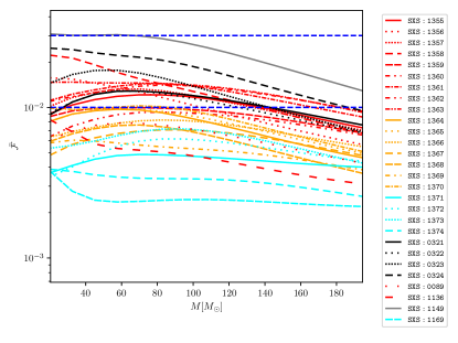
SUPPLEMENTARY FIGURE 1: EOB/NR unfaithfulness for mildly eccentric systems. Comparison between 28 mildly eccentric NR simulations from the SXS catalog[SXS:catalog] and the eccentric TEOBResumS. These mismatches improve and extend those computed in previous work[30].

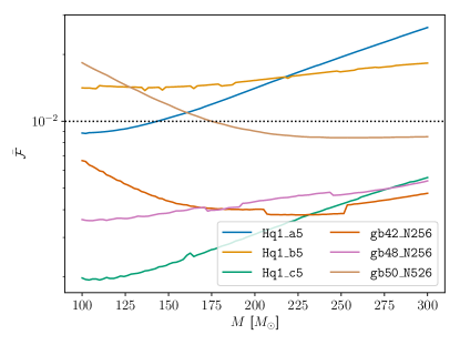
SUPPLEMENTARY FIGURE 2: EOB/NR unfaithfulness for highly eccentric and capture configurations. Comparison between the NR simulations of Table 1, produced for this work, and the eccentric TEOBResumS. We consider frequencies between $11$ and $512$ Hz, use the Hanford PSD of GW190521 and compute $\bar{\mathcal{F}}$ for systems with masses $M\in[100,300]M_{\odot}$.

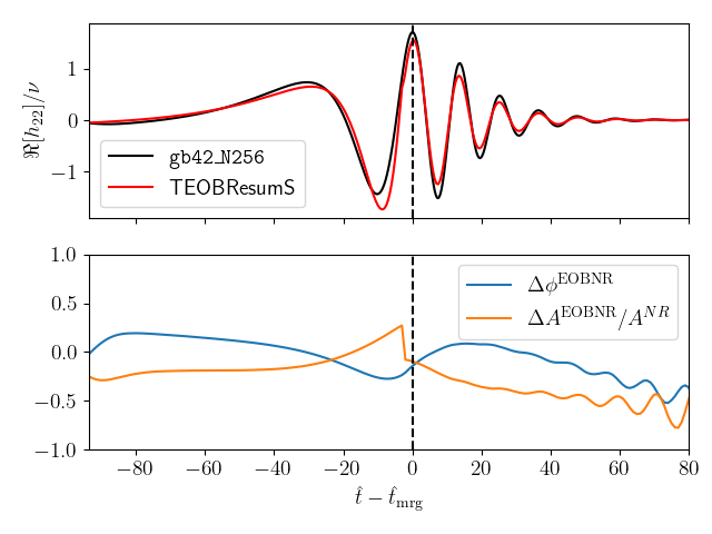
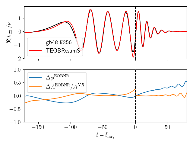
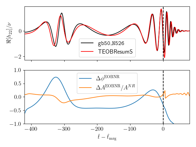
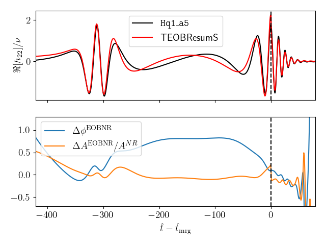
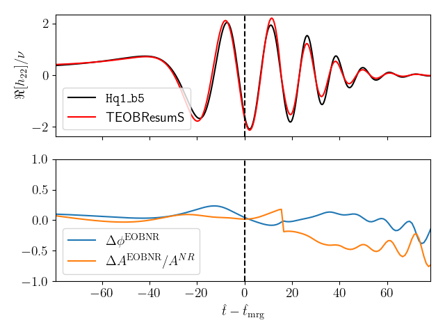
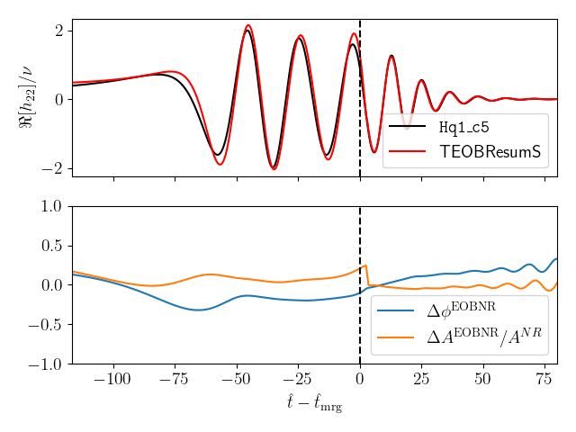
SUPPLEMENTARY FIGURE 3: Time-domain EOB/NR phasing comparison. Comparing the Numerical Relativity waveforms of Table 1 to the analytical ones obtained using the eccentric TEOBResumS. For each configuration, the top panel displays the amplitude and the real part of the dominant multipole $h_{22}$, while the bottom panel shows the phase difference $\Delta\phi^{\rm EOBNR}=\phi^{\rm EOB}-\phi^{\rm NR}$ and the relative amplitude difference $\Delta A^{\rm EOBNR}/A^{\rm NR}=(A^{\rm EOB}-A^{\rm NR})/A^{\rm NR}$. Despite the lack of NQC corrections or of an hyperbolic-NR-informed ringdown, TEOBResumS quantitatively captures the NR waveform for any configuration.

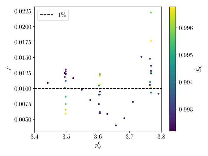
SUPPLEMENTARY FIGURE 4: EOB/NR unfaithfulness for the highly eccentric NR waveforms from the RIT catalog. We compare 46 nonspinning highly eccentric datasets from RIT[47] with the eccentric TEOBResumS model. We select only those systems whose best matching EOB initial conditions, estimated via Eq. (S1), fall inside the posterior samples. We consider frequencies between $11$ and $512$ Hz, use the Hanford PSD of GW190521 and compute $\bar{\mathcal{F}}$ with fixed total mass $M=250M_{\odot}$.

ID	$\hat{r}_{0}^{\rm EOB}$	$\hat{E}^{\rm EOB}$	$\hat{p}_{\varphi}^{\rm EOB}$	$\hat{E}^{\rm EOB}_{\rm opt}$	$\hat{p}_{\varphi\;\rm opt}^{\rm EOB}$	$\Delta E/E[\%]$	$\Delta p_{\varphi}/p_{\varphi}[\%]$
$\tt Hq1\_a5$	$100.000$	$1.003$	$3.970$	$1.005$	$3.987$	$-0.132$	$-0.440$
$\tt Hq1\_b5$	$100.000$	$1.008$	$3.970$	$1.010$	$4.049$	$-0.192$	$-2.000$
$\tt Hq1\_c5$	$100.000$	$1.007$	$3.970$	$1.015$	$4.181$	$-0.799$	$-5.323$
$\tt gb42\_N256$	$20.842$	$0.994$	$3.305$	$0.994$	$3.238$	$0.018$	$2.033$
$\tt gb48\_N256$	$20.869$	$0.994$	$3.671$	$0.997$	$3.762$	$-0.267$	$-2.476$
$\tt gb50\_N526$	$20.878$	$0.994$	$3.784$	$0.993$	$3.771$	$0.131$	$0.342$

SUPPLEMENTARY TABLE 1: EOB initial data to match NR simulations. The values correspond to the equal-mass, nonspinning NR data of Figs. 2 and 3. The first column of the table reports the configuration label. The quantities $\hat{r}_{0}^{\rm EOB}$,$\hat{E}^{\rm EOB}$ and $\hat{p}_{\varphi}^{\rm EOB}$ are the initial EOB radial separation, initial energy and initial angular momentum obtained by mapping the initial position and momenta of the punctures into EOB coordinates via the 2PN coordinate transformation between ADM and EOB coordinates[Bini:2012ji]. The quantities $\hat{E}^{\rm EOB}_{\rm opt}$ and $\hat{p}_{\varphi\;\rm opt}^{\rm EOB}{}$, instead, are the corresponding values which minimize the EOB/NR mismatch at $M=250M_{\odot}$. The last two columns report the corresponding relative differences.

5.4 Injection-recovery studies

To better understand the increase in $\log(\mathcal{L})_{\rm max}$ and Bayes’ factor observed in the main text we perform two additional ”injection-recovery” studies:

1. Using the NRSur7dq4 waveform model, we simulate a quasicircular signal with the maximum likelihood parameters recovered from GW190521 into gaussian noise generated with the PSD estimated close to the event, and recover it with both NRSur7dq4 and ${\tt TEOBResumS}$

2. We perform a self-consistency test: we simulate and recover a signal with the hyperbolic model employed in the main text, ${\tt TEOBResumS}$, with parameters similar to GW190521.

In all cases we adopt the same PE settings and priors as the ones used in the analysis shown in the main paper.

Our results for the first injection-recovery test are reported in Table 2. Both the maximum likelihood and the Bayes Factor recovered with NRSur7dq4 are slightly larger than those obtained with ${\tt TEOBResumS}$. On the one hand, this indicates that the significant increase in Bayes Factor and likelihood we observe in our analyses is not obtained when the real signal is generated by a precessing, quasi circular source. On the other hand, it also shows how short-lived precessing signals can be matched reasonably well also by dynamical-capture waveform models, i.e. the symmetric scenario with respect to the one discussed in[18]. Note that, due to the specific noise realization, at times the injected parameters lie just outside the $90\%$ credible levels even when the recovery is performed with the surrogate.

Table 3, instead, displays the injected and recovered parameters obtained from our second injection-recovery test. All the recovered parameters lie, as expected, well within the $90\%$ intervals. This indicates that our inference framework (including the model implementation) behaves correctly, and is able to recover the simulated parameters in spite of the complicated structure of the $(E,p_{\varphi})$ parameter space.

	Injected (NRSur7dq4)	NRSur7dq4	TEOBResumS
$m_{1}$ [$M_{\odot}$]	$135$	$155^{+19}_{-19}$	$145^{+21}_{-20}$
$m_{2}$ [$M_{\odot}$]	$125$	$89^{+36}_{-34}$	$88^{+28}_{-36}$
$M$ [$M_{\odot}$]	$260$	$244^{+38}_{-36}$	$232^{+15}_{-20}$
$m_{1}^{\rm source}$ [$M_{\odot}$]	$90.01$	$92^{+19}_{-20}$	$72^{+26}_{-14}$
$m_{2}^{\rm source}$ [$M_{\odot}$]	$83.397$	$52^{+21}_{-18}$	$43^{+17}_{-16}$
$M_{\rm source}$ [$M_{\odot}$]	$173.40$	$141^{+31}_{-21}$	$115^{+29}_{-16}$
$m_{2}/m_{1}\leq 1$	$0.92$	$0.57^{+0.28}_{-0.23}$	$0.61^{+0.31}_{-0.29}$
$\chi_{\rm eff}$	$-0.29$	$-0.18^{+0.43}_{-0.41}$	–
$\chi_{\rm p}$	$0.79$	$0.51^{+0.33}_{-0.38}$	–
$E^{0}/M$	–	–	$1.010^{+0.013}_{-0.009}$
${p_{\varphi}^{0}}$	–	–	$4.08^{+0.32}_{-0.27}$
$D_{L}$ [Mpc]	$2935$	$4390^{+3370}_{-2060}$	$6950^{+2590}_{-3290}$
$\log({\cal L})_{\rm max}$	–	$56.70$	$52.84$
$\log{\cal B}^{\rm signal}_{\rm noise}$	–	$29.65$	$28.43$

SUPPLEMENTARY TABLE 2: First injection-recovery study. Results of our ${\tt NRSur7dq4}-{\tt NRSur7dq4}$ and ${\tt NRSur7dq4}-{\tt TEOBResumS}$ injection-recovery studies in GW190521 gaussian noise. Posteriors are expressed, as is standard, via their median and $90\%$ credible intervals. Notably, the $\log({\cal L})_{\rm max}$ and $\log{\cal B}^{\rm signal}_{\rm noise}$ recovered with the NR surrogate are higher than those obtained with the hyperbolic model.

	Injected (TEOBResumS)	TEOBResumS
$m_{1}^{\rm source}$ [$M_{\odot}$]	$81$	$93^{+22}_{-14}$
$m_{2}^{\rm source}$ [$M_{\odot}$]	$71$	$60^{+14}_{-18}$
$M_{\rm source}$ [$M_{\odot}$]	$152$	$153^{+16}_{-10}$
$m_{2}/m_{1}\leq 1$	$0.88$	$0.64^{+0.25}_{-0.27}$
$E^{0}/M$	$1.012$	$1.010^{+0.007}_{-0.008}$
${p_{\varphi}^{0}}$	$4.21$	$4.04^{+0.27}_{-0.29}$
$D_{L}$ [Mpc]	$3000$	$2400^{+790}_{-930}$
$\log({\cal L})_{\rm max}$	–	$316.84$
$\log{\cal B}^{\rm signal}_{\rm noise}$	–	$282.44$

SUPPLEMENTARY TABLE 3: Second injection-recovery study. Results of our ${\tt TEOBResumS}-{\tt TEOBResumS}$ injection-recovery experiment in GW190521 gaussian noise. Posteriors are expressed, as is standard, via their median and $90\%$ credible intervals. The injected true values all fall within the $90\%$ intervals.

plain supp.bbl

References

- [1] Aasi, J. et al. Advanced LIGO. Class. Quant. Grav. 32, 074001 (2015). 1411.4547.
- [2] Acernese, F. et al. Advanced Virgo: a second-generation interferometric gravitational wave detector. Class. Quant. Grav. 32, 024001 (2015). 1408.3978.
- [3] Abbott, R. et al. GWTC-3: Compact Binary Coalescences Observed by LIGO and Virgo During the Second Part of the Third Observing Run (2021). 2111.03606.
- [4] Abbott, R. et al. GW190521: A Binary Black Hole Merger with a Total Mass of 150 M. Phys. Rev. Lett. 125, 101102 (2020). 2009.01075.
- [5] Abbott, R. et al. Properties and astrophysical implications of the 150 Msun binary black hole merger GW190521. Astrophys. J. Lett. 900, L13 (2020). 2009.01190.
- [6] Abbott, R. et al. Population Properties of Compact Objects from the Second LIGO-Virgo Gravitational-Wave Transient Catalog. Astrophys. J. Lett. 913, L7 (2021). 2010.14533.
- [7] González, E. et al. Intermediate-mass Black Holes from High Massive-star Binary Fractions in Young Star Clusters. Astrophys. J. Lett. 908, L29 (2021). 2012.10497.
- [8] Belczynski, K. The most ordinary formation of the most unusual double black hole merger. Astrophys. J. Lett. 905, L15 (2020). 2009.13526.
- [9] Mapelli, M. et al. Hierarchical black hole mergers in young, globular and nuclear star clusters: the effect of metallicity, spin and cluster properties. Mon. Not. R. Astron. Soc. 505, 339–358 (2021). 2103.05016.
- [10] Sedda, M. A. et al. Breaching the limit: formation of GW190521-like and IMBH mergers in young massive clusters (2021). 2105.07003.
- [11] Tagawa, H., Haiman, Z., Bartos, I., Kocsis, B. & Omukai, K. Signatures of Hierarchical Mergers in Black Hole Spin and Mass distribution (2021). 2104.09510.
- [12] Dall’Amico, M. et al. GW190521 formation via three-body encounters in young massive star clusters (2021). 2105.12757.
- [13] Fragione, G., Loeb, A. & Rasio, F. A. On the Origin of GW190521-like Events from Repeated Black Hole Mergers in Star Clusters. Astrophys. J. Lett. 902, L26 (2020). 2009.05065.
- [14] Fragione, G., Kocsis, B., Rasio, F. A. & Silk, J. Repeated mergers, mass-gap black holes, and formation of intermediate-mass black holes in nuclear star clusters. arXiv e-prints arXiv:2107.04639 (2021). 2107.04639.
- [15] Gayathri, V. et al. Eccentricity estimate for black hole mergers with numerical relativity simulations. Nature Astron. 6, 344–349 (2022). 2009.05461.
- [16] Romero-Shaw, I. M., Lasky, P. D., Thrane, E. & Bustillo, J. C. GW190521: orbital eccentricity and signatures of dynamical formation in a binary black hole merger signal. Astrophys. J. Lett. 903, L5 (2020). 2009.04771.
- [17] Bustillo, J. C., Sanchis-Gual, N., Torres-Forné, A. & Font, J. A. Confusing Head-On Collisions with Precessing Intermediate-Mass Binary Black Hole Mergers. Phys. Rev. Lett. 126, 201101 (2021). 2009.01066.
- [18] Bustillo, J. C. et al. GW190521 as a Merger of Proca Stars: A Potential New Vector Boson of eV. Phys. Rev. Lett. 126, 081101 (2021). 2009.05376.
- [19] Shibata, M., Kiuchi, K., Fujibayashi, S. & Sekiguchi, Y. Alternative possibility of GW190521: Gravitational waves from high-mass black hole-disk systems. Phys. Rev. D 103, 063037 (2021). 2101.05440.
- [20] Nitz, A. H. & Capano, C. D. GW190521 may be an intermediate mass ratio inspiral. Astrophys. J. Lett. 907, L9 (2021). 2010.12558.
- [21] Estellés, H. et al. A detailed analysis of GW190521 with phenomenological waveform models (2021). 2105.06360.
- [22] East, W. E., McWilliams, S. T., Levin, J. & Pretorius, F. Observing complete gravitational wave signals from dynamical capture binaries. Phys. Rev. D87, 043004 (2013). 1212.0837.
- [23] Gold, R. & Brügmann, B. Eccentric black hole mergers and zoom-whirl behavior from elliptic inspirals to hyperbolic encounters. Phys. Rev. D88, 064051 (2013). 1209.4085.
- [24] Loutrel, N. Repeated Bursts: Gravitational Waves from Highly Eccentric Binaries (2020). 2009.11332.
- [25] Rasskazov, A. & Kocsis, B. The rate of stellar mass black hole scattering in galactic nuclei. Astrophys. J. 881, 20 (2019). 1902.03242.
- [26] Tagawa, H., Haiman, Z. & Kocsis, B. Formation and Evolution of Compact Object Binaries in AGN Disks. Astrophys. J. 898, 25 (2020). 1912.08218.
- [27] Rodriguez, C. L. et al. Post-Newtonian Dynamics in Dense Star Clusters: Formation, Masses, and Merger Rates of Highly-Eccentric Black Hole Binaries. Phys. Rev. D 98, 123005 (2018). 1811.04926.
- [28] Mukherjee, S., Mitra, S. & Chatterjee, S. Detectability of hyperbolic encounters of compact stars with ground-based gravitational waves detectors (2020). 2010.00916.
- [29] Mandel, I. & Broekgaarden, F. S. Rates of Compact Object Coalescences (2021). 2107.14239.
- [30] Chiaramello, D. & Nagar, A. Faithful analytical effective-one-body waveform model for spin-aligned, moderately eccentric, coalescing black hole binaries. Phys. Rev. D 101, 101501 (2020). 2001.11736.
- [31] Nagar, A., Rettegno, P., Gamba, R. & Bernuzzi, S. Effective-one-body waveforms from dynamical captures in black hole binaries. Phys. Rev. D 103, 064013 (2021). 2009.12857.
- [32] Buonanno, A. & Damour, T. Effective one-body approach to general relativistic two-body dynamics. Phys. Rev. D59, 084006 (1999). gr-qc/9811091.
- [33] Blanchet, L. Gravitational Radiation from Post-Newtonian Sources and Inspiralling Compact Binaries. Living Rev. Relativity 17, 2 (2014). 1310.1528.
- [34] Schaefer, G. & Jaranowski, P. Hamiltonian formulation of general relativity and post-Newtonian dynamics of compact binaries. Living Rev. Rel. 21, 7 (2018). 1805.07240.
- [35] Nagar, A., Riemenschneider, G., Pratten, G., Rettegno, P. & Messina, F. Multipolar effective one body waveform model for spin-aligned black hole binaries. Phys. Rev. D 102, 024077 (2020). 2001.09082.
- [36] Pretorius, F. & Khurana, D. Black hole mergers and unstable circular orbits. Class.Quant.Grav. 24, S83–S108 (2007). gr-qc/0702084.
- [37] Healy, J., Levin, J. & Shoemaker, D. Zoom-Whirl Orbits in Black Hole Binaries. Phys.Rev.Lett. 103, 131101 (2009). 0907.0671.
- [38] Sperhake, U. et al. Cross section, final spin and zoom-whirl behavior in high-energy black hole collisions. Phys.Rev.Lett. 103, 131102 (2009). 0907.1252.
- [39] Damour, T. et al. Strong-Field Scattering of Two Black Holes: Numerics Versus Analytics (2014). 1402.7307.
- [40] Hopper, S., Nagar, A. & Rettegno, P. Strong-field scattering of two spinning black holes: Numerics versus Analytics (2022). 2204.10299.
- [41] Aghanim, N. et al. Planck 2018 results. VI. Cosmological parameters. Astron. Astrophys. 641, A6 (2020). 1807.06209.
- [42] Varma, V. et al. Surrogate models for precessing binary black hole simulations with unequal masses. Phys. Rev. Research. 1, 033015 (2019). 1905.09300.
- [43] Akcay, S., Gamba, R. & Bernuzzi, S. A hybrid post-Newtonian – effective-one-body scheme for spin-precessing compact-binary waveforms. Phys. Rev. D 103, 024014 (2021). 2005.05338.
- [44] Gamba, R., Akçay, S., Bernuzzi, S. & Williams, J. Effective-one-body waveforms for precessing coalescing compact binaries with post-Newtonian twist. Phys. Rev. D 106, 024020 (2022). 2111.03675.
- [45] Breschi, M., Gamba, R. & Bernuzzi, S. Bayesian inference of multimessenger astrophysical data: Methods and applications to gravitational waves. Phys. Rev. D 104, 042001 (2021). 2102.00017.
- [46] Nagar, A., Bonino, A. & Rettegno, P. Effective one-body multipolar waveform model for spin-aligned, quasicircular, eccentric, hyperbolic black hole binaries. Phys. Rev. D 103, 104021 (2021). 2101.08624.
- [47] Healy, J. & Lousto, C. O. The Fourth RIT binary black hole simulations catalog: Extension to Eccentric Orbits (2022). 2202.00018.
- [48] Harms, E., Bernuzzi, S., Nagar, A. & Zenginoglu, A. A new gravitational wave generation algorithm for particle perturbations of the Kerr spacetime. Class.Quant.Grav. 31, 245004 (2014). 1406.5983.
- [49] Albanesi, S., Nagar, A. & Bernuzzi, S. Effective one-body model for extreme-mass-ratio spinning binaries on eccentric equatorial orbits: Testing radiation reaction and waveform. Phys. Rev. D 104, 024067 (2021). 2104.10559.
- [50] Abbott, R. et al. Open data from the first and second observing runs of Advanced LIGO and Advanced Virgo (2019). 1912.11716.
- [51] Speagle, J. S. dynesty: a dynamic nested sampling package for estimating bayesian posteriors and evidences. Monthly Notices of the Royal Astronomical Society 493, 3132?3158 (2020). URL http://dx.doi.org/10.1093/mnras/staa278.
- [52] Cao, Z. & Han, W.-B. Waveform model for an eccentric binary black hole based on the effective-one-body-numerical-relativity formalism. Phys. Rev. D96, 044028 (2017). 1708.00166.