Strong-field scattering of two spinning black holes: Numerics versus Analytics

Abstract

We present new Numerical Relativity calculations of the scattering angle $\chi$ between two, equal-mass, black holes on hyperbolic-like orbits. We build upon previous work considering, for the first time, spinning black holes, with equal spins either aligned or antialigned with the orbital angular momentum. We detail the numerical techniques used in the computation of $\chi$. Special care is taken in estimating error uncertainties on the quantities computed. The numerical values are compared with analytical predictions obtained using a new, state-of-the-art, effective one body model valid on generic orbits that incorporates post-Newtonian analytic information up to 5PN in the nonspinning, conservative sector and that has been additionally informed by Numerical Relativity simulations of quasi-circular coalescing black hole binaries. Our results indicate that the spin sector of the analytic model should be improved further in order to achieve satisfactory consistency with the most relativistic spinning configurations.

I Introduction

Motivated by recent observational hints for eccentric and hyperbolic binary black hole (BBH) mergers in some LIGO-Virgo events Abbott et al. (2020); Gayathri et al. (2020); Gamba et al. (2021) and by future prospect of detecting binary sources on generic orbits with LISA Amaro-Seoane et al. (2017); Babak et al. (2017); Gair et al. (2017), the analytical relativity community is intensifying the efforts in building up accurate gravitational-wave (GW) models for noncircularized coalescing compact binaries Hinder et al. (2017); Hinderer and Babak (2017); Chiaramello and Nagar (2020); Loutrel (2020); Nagar et al. (2021a); Islam et al. (2021); Nagar et al. (2021b); Nagar and Rettegno (2021); Albanesi et al. (2021); Liu et al. (2021); Yun et al. (2021); Tucker and Will (2021); Setyawati and Ohme (2021); Khalil et al. (2021); Ramos-Buades et al. (2021); Placidi et al. (2021). The effective-one-body (EOB) framework Buonanno and Damour (1999, 2000); Damour et al. (2000); Damour (2001); Damour et al. (2015) offers a theoretically complete method for a unified description of different classes of astrophysical binaries, from the comparable masses to the intermediate and extreme mass-ratio regimes, and for incorporating the fast motion and ringdown dynamics.

Among the noncircular configurations, the case of hyperbolic scattering and hyperbolic capture is the one computationally more challenging. On the analytical side, after the pioneering work of Ref. East et al. (2013), Ref. Nagar et al. (2021a) gave a comprehensive treatment of the phenomenon within the EOB model, constructing a complete waveform, through merger and ringdown, that was used in the analysis of GW190521 Gamba et al. (2021). The above-mentioned model was then improved in Refs. Nagar et al. (2021b); Nagar and Rettegno (2021). At a more fundamental level, the calculation of the gravitational scattering angle has received more and more attention in recent years in the context of the formulation of an EOB model making use of the post-Minkowskian approximation Damour (2016, 2018, 2020a); Bern et al. (2019); Damour (2020b); Kälin et al. (2020); Bini et al. (2021a, b); Bern et al. (2021); Dlapa et al. (2021a, b); Manohar et al. (2022); Khalil et al. (2022); Buonanno et al. (2022).

On the Numerical Relativity (NR) side, after the pioneering work of Gold and Bruegmann Gold and Brügmann (2013) on elliptic inspirals and hyperbolic encounters, Ref. Damour et al. (2014) presented the first, and so far only, computation of the scattering angle $\chi$ from equal-mass nonspinning black holes (BHs) on hyperbolic-like orbits. Scattering configurations were also considered in Ref. Nelson et al. (2019), although the focus of the paper was on the spin-up of the two BHs induced by the close encounter and no calculation of $\chi$ was reported. In this paper we extend the parameter space explored in Ref. Damour et al. (2014), presenting the computation of the scattering angle for 32 new equal-mass, equal-spin (with spin aligned with the orbital angular momentum) configurations. Of these 32 dataset, only 5 are nonspinning. In Ref. Damour et al. (2014) the initial energy of the configurations was constant and the starting angular momentum varied. Here, for each value of the spin, we (approximately) fix the initial angular momentum and progressively increase the energy. Similarly to Ref. Damour et al. (2014), the numerical scattering angles are compared with the analytical calculation obtained using the state-of-the-art TEOBResumS model for generic configurations of Ref. Nagar and Rettegno (2021).

This paper is organized as follows. In Sec. II we describe our NR simulations, focusing in particular on the computation of the scattering angle from the extrapolation of the puncture trajectories and on the calculation of the energy and angular momentum losses during the process. The calculation of the scattering angle is reported in Sec. III, where it is also compared with the EOB predictions. Our conclusions are collected in Sec. IV.

We use geometrized units with $c=G=1$.

II Numerical Relativity: scattering angle, waveforms and fluxes

We report here the results of a large number of NR simulation performed at the beginning of 2016 and never published since. They were done using the November 2015 (Sommerville) release of the the Einstein Toolkit Loffler et al. (2012); Ein . As such, the techniques used here are similar to those behind the results of Ref. Damour et al. (2014), and thus the current paper should be seen as a complement to the information reported there.

Table 1: Initial data for the NR simulations. From left to right the columns report: configuration number; dimensionless spin; $(p_{x},p_{y})$ in-plane components of the momentum $\vec{p}_{1}$ of the $m_{1}$ BH located at $x=X=50M$ (note that $\vec{p_{2}}=-\vec{p}_{1}$); initial ADM energy, initial ADM total angular momentum and initial ADM orbital angular momentum.

$\#$	$S_{i}/m_{i}^{2}$	$p_{x}/M$	$p_{y}/M$	$E_{\rm ADM}/M$	$J_{\rm ADM}/M^{2}$	$J_{\rm ADM}^{\rm orb}/M^{2}$
1	0	$-0.05942506$	0.01151993	1.00457189170793	1.15198647944995	1.15198647944995
2	0	$-0.09423272$	0.01151978	1.0148091006975	1.15195577447483	1.15195577447483
3	0	$-0.10755541$	0.01151963	1.01992105354885	1.15192562845173	1.15192562845173
4	0	$-0.11943931$	0.01151938	1.02502400428497	1.15187555184956	1.15187555184956
5	0	$-0.14030562$	0.01151787	1.03513920185028	1.15157506725085	1.15157506725085
s1	0.6	$-0.11576611$	0.01216040	1.07665374989219	1.6179219954769	1.28364059145275
s2	0.6	$-0.12796939$	0.01215992	1.08202144718546	1.61779453645181	1.28353946693697
s3	0.6	$-0.13914499$	0.01215957	1.08740041845793	1.6177018945377	1.2834659659142
s4	0.6	$-0.14952098$	0.01215909	1.09276714425576	1.61757391942674	1.28336443194187
s5	0.6	$-0.16845199$	0.01215769	1.10345914737548	1.61720025417128	1.28306797025159
s6	0.6	$-0.20127763$	0.01215111	1.12448714803832	1.61545155902268	1.28160813445288
s7	0.6	$-0.22973878$	0.01214243	1.14529304319858	1.61314401406252	1.27974086738477
s8	0.4	$-0.11133090$	0.01177667	1.04267905040057	1.41285715786028	1.20385461971527
s9	0.4	$-0.12329970$	0.01177641	1.04789622892359	1.41291760105672	1.20390612161046
s10	0.4	$-0.13424207$	0.01177617	1.05311363730914	1.41279793409858	1.20380415686506
s11	0.4	$-0.14439149$	0.01177592	1.05833035249639	1.41273744727074	1.20375261779282
s12	0.4	$-0.16289572$	0.01177552	1.0687733648426	1.41264358611283	1.20367264142158
s13	0.4	$-0.17958219$	0.01177309	1.07902769262705	1.41205766742487	1.20317339709575
s14	0.4	$-0.19493661$	0.01177061	1.08927474892939	1.41146428986134	1.2026677972783
s15	0.2	$-0.09514373$	0.01158044	1.02015292937479	1.26517182375897	1.16411976115842
s16	0.2	$-0.12037734$	0.01158021	1.03043668219383	1.26512069418535	1.16407271541655
s17	0.2	$-0.14130345$	0.01157971	1.04069639252575	1.2650121280105	1.16397282066142
s18	0.2	$-0.15961623$	0.01157844	1.05088513370079	1.26473486730472	1.16371770537942
s19	$-0.2$	$-0.12027829$	$0.01258520$	1.03041733634713	1.16402900625683	1.26507319082773
s20	$-0.2$	$-0.14121083$	$0.01258398$	1.04062105981093	1.16380431415062	1.26482899419842
s21	$-0.2$	$-0.15948828$	$0.01257917$	1.05052233902211	1.16291434885511	1.263861774971
s22	$-0.4$	$-0.12308769$	0.01382007	1.04783052701748	1.20370366381241	1.41267999433539
s23	$-0.4$	$-0.14420487$	0.01381917	1.0582400621434	1.20354723275444	1.41249640510764
s24	$-0.4$	$-0.16269187$	0.01381569	1.06844864874712	1.20294134980541	1.41178533414662
s25	$-0.6$	$-0.12761312$	0.01532347	1.08180243941042	1.28301992700588	1.61713969966367
s26	$-0.6$	$-0.16815583$	0.01531961	1.10316051991281	1.28237359478648	1.61632505176213
s27	$-0.6$	$-0.20054310$	0.01527546	1.12155004323926	1.27499394723474	1.60702362099378

II.1 Initial data

The initial data of the Bowen-York form for the two BHs is provided by the TwoPunctures Ansorg et al. (2004) thorn in the Einstein Toolkit. While the thorn takes as input gauge dependent quantities such as initial separation and momenta, we will eventually need gauge-invariant quantities [namely Arnowitt-Deser-Misner (ADM) energy and angular momentum] to provide meaningful comparisons with the EOB results, following the same rational of Ref. Damour et al. (2014). To have this, we proceeded as follows. The BHs start on the $x$-axis with initial positions designated by $\pm X$ and initial momenta in the plane $(p_{x},p_{y})$. The ADM orbital angular momentum is given by

$$J_{\rm ADM}=2X|p_{y}|.$$ (1)

For all simulations we use $X=50M$, while $(p_{x},p_{y},E_{\rm ADM},J_{\rm ADM})$ are listed in Table 1. For each run, we chose a doublet of $(E_{\rm ADM},J_{\rm ADM})$. In particular, we keep the same value of $p_{y}$ for a given spin and then we determine $p_{x}$ through the iterative procedure to obtain the target value of $E_{\rm ADM}$. That procedure is a root-finding routine wherein we solved for the initial data repeatedly until we had the correct input quantities corresponding to those gauge invariant quantities.

Note that, although the data in Table 1 are those actually used to start the simulations, these are not the quantities of interest to compare the NR with the EOB scattering angle. To this aim we will need to subtract from the initial ADM quantities the energy and angular momentum losses due to the junk radiation, analogously to what done in Ref. Damour et al. (2014). We shall come back to this below.

II.2 Mesh refinement and boundary conditions

A major challenge of scattering simulations is the need for a very large grid. Our BHs start $100M$ apart and end even more widely separated. The large final separation is partly due to a desire for an accurate angle of deflection. Additionally, we must run our simulations long enough for radiation from the encounter to reach the extraction spheres. We ran our simulations on very large computational domains. They were all performed in cubes with $(x,y,z)$ coordinates, each running from $-5033M$ to $5033M$. In order to accommodate such a large grid we used 13 layers of box-in-box mesh refinement implemented by the Carpet thorn Schnetter et al. (2004); Car . The outer 6 layers were static, while the inner 7 layers tracked the punctures. We used radiative boundary conditions although we note that our grid was specifically designed to be large enough so reflections off the outer boundary did not have time to return and interfere with either the punctures or wave extraction.

II.3 Calculation of the deflection angle through extrapolation of the BHs trajectories

Let us focus first on the description of the procedure adopted to the computation of the deflection angle, which is our main observable of interest. Since we are limited to a finite-size grid, the deflection angle is obtained by extrapolating the puncture trajectories to infinity. For any given run, we perform the following steps:

1. We write the relative motion of the puncture tracks as $(x,y)=(x_{1},y_{1})-(x_{2},y_{2})$. Since the BH spins will always be either aligned or anti-aligned with the orbital angular momentum, the BHs are never out the $(x,y)$ plane.

2. Convert the relative motion to standard polar coordinates $(r,\theta)=(\sqrt{x^{2}+y^{2}},\arctan(y/x))$.

3. Truncate the $(r,\theta)$ data at both the beginning and the end of the simulations. This way we have incoming and outgoing legs representing the motion before and after the strong field interaction. We denote these data sets as $(r_{\rm in},\theta_{\rm in})$ and $(r_{\rm out},\theta_{\rm out})$, respectively. In practice, we find that a separation of $r=25M$ is a reasonable cutoff for the strong field.

4. Perform a least-squares fit on the incoming and outgoing legs to find power series representations of $\theta_{\rm in}$ and $\theta_{\rm out}$ in $1/r$. We repeat this fit for a range of polynomial orders. We have experimented with several different maximum polynomial orders and find that cubic and higher orders give consistent results in the final answer.

5. Extrapolate each of the incoming and outgoing angles to infinite separation by taking the $1/r\to 0$ limits of the the fits (i.e., take the constant terms in the polynomials), providing $\theta_{\rm in}^{\infty}$ and $\theta_{\rm out}^{\infty}$. We choose the extrapolated angles from 4th-order polynomials (noting that polynomials of 3rd-6th order give consistent results within our uncertainty ranges).

6. Make (conservative) estimates for the errors in $\theta_{\rm in}^{\infty}$ and $\theta_{\rm out}^{\infty}$. To find the error in $\theta_{\rm in}^{\infty}$ (e.g.) we first perform our least-squares fit using 1st-4th order polynomials. We then perform the extrapolation for each polynomial and take the error to be the range of the results.

7. Report the final angle of deflection (in degrees) as $\chi=\theta_{\rm out}^{\infty}-\theta_{\rm in}^{\infty}-180$. We take the final error in $\chi$ to be the norm of the errors in $\theta_{\rm ins}^{\infty}$ and $\theta_{\rm out}^{\infty}$.

The numerical results for the scattering angles, $\chi^{\rm NR}$, are reported in the ninth column of Table 2 (nonspinning configurations) and in the tenth column of Table 3 (spinning configurations). The values come with error bars, that range from a few $\%$’s to well below $1\%$, depending on the dataset. The total uncertainty estimate is rather conservative and it is done as follows. Each configuration is simulated at two different resolutions and for each one we compute the scattering angle with the procedure mentioned above. The finite-difference uncertainty is thus obtained by simply taking the difference between the angles obtained with the two resolution. To this value, we additionally add, in quadrature, the uncertainty related to the extrapolation procedure mentioned above. Note that for each value of the spin we considered configurations at (approximately) constant orbital angular momentum and we increased progressively the energy. Configuration #s7 of Table 3 is rather extreme and close to the zoom-whirl behavior, since we obtain $\chi^{\rm NR}=371.5(9.9)$ rad. We performed multiple simulations with only slightly more energy, each leading to capture.

Table 2: Comparison between EOB and NR scattering angle for equal-mass, nonspinning configurations. The initial angular momentum is kept approximately constant, while the initial energy is progressively raised. From left to right the columns report: the ordering number; the minimum EOB distance $r_{\rm min}^{\rm EOB}$; the initial energy $\hat{E}^{\rm NR}_{\rm in}=E^{\rm NR}_{\rm in}/M$; the initial orbital angular momentum $\hat{J}^{\rm NR}_{\rm in,orb}=J^{\rm NR}_{\rm in,orb}/M^{2}$; the NR and EOB radiated energies, $(\Delta\hat{E}^{\rm NR},\Delta\hat{E}^{\rm EOB})$; the NR and EOB radiated angular momentum, $(\Delta\hat{J}^{\rm NR},\Delta\hat{J}^{\rm EOB})$; the NR and EOB scattering angles $(\chi^{\rm NR},\chi^{\rm EOB})$ and their fractional difference $\hat{\Delta}\chi^{\rm NREOB}\equiv|\chi^{\rm NR}-\chi^{\rm EOB}|/\chi^{\rm NR}$.

$\#$	$r_{\rm min}^{\rm EOB}$	$\hat{E}^{\rm NR}_{\rm in}$	$\hat{J}^{\rm NR}_{\rm in,orb}$	$\Delta\hat{E}^{\rm NR}$	$\Delta\hat{E}^{\rm EOB}$	$\Delta\hat{J}^{\rm NR}$	$\Delta\hat{J}^{\rm EOB}$	$\chi^{\rm NR}$ [deg]	$\chi^{\rm EOB}$[deg]	$\hat{\Delta}\chi^{\rm NREOB}[\%]$
1	6.70	1.0045678(42)	1.1520071(73)	0.001625(16)	0.0014	0.034511(71)	0.0278	201.9(4.8)	200.5173	0.69
2	5.02	1.0147923(76)	1.151918(16)	0.004925(30)	0.0042	0.069504(39)	0.0549	195.9(1.3)	194.5465	0.71
3	4.46	1.0198847(82)	1.151895(11)	0.00793(34)	0.0068	0.09456(70)	0.0757	207.03(99)	207.0698	0.02
4	3.97	1.024959(12)	1.151845(12)	0.01194(27)	0.0109	0.1252(10)	0.1055	225.54(87)	229.0237	1.54
5	3.13	1.035031(27)	1.1515366(78)	0.0281(11)	0.0306	0.2220(64)	0.2283	307.13(88)	345.9284	12.63

Table 3: Comparison between EOB and NR scattering angle for equal-mass, equal-spin BBHs. The column entries are the same of Table 2, with the addition of the spin parameter $a/M$. For each dimensionless spin value of $S_{1,2}/m_{1,2}^{2}$, the initial angular momentum is almost constant while the energy is changed. When TEOBResumS predicts a plunge instead of a scattering, the EOB quantities cannot be meaningfully compared and are hence substituted by dots. This happens for the most energetic systems.

$\#$	$S_{i}/m_{i}^{2}$	$r_{\rm min}^{\rm EOB}$	$\hat{E}^{\rm NR}_{\rm in}$	$\hat{J}^{\rm NR}_{\rm in,orb}$	$\Delta\hat{E}^{\rm NR}$	$\Delta\hat{E}^{\rm EOB}$	$\Delta\hat{J}^{\rm NR}$	$\Delta\hat{J}^{\rm EOB}$	$\chi^{\rm NR}$ [deg]	$\chi^{\rm EOB}$[deg]	$\hat{\Delta}\chi^{\rm NREOB}[\%]$
s1	0.6	3.25	1.076631(25)	1.283562(22)	0.004530(90)	0.009	0.06944(42)	0.0835	153.1(1.3)	157.2555	2.70
s2	0.6	3.09	1.081965(13)	1.283473(27)	0.00636(16)	0.0109	0.08527(37)	0.0954	155.6(1.1)	165.6316	6.43
s3	0.6	2.94	1.087309(15)	1.2834073(65)	0.008449(88)	0.0134	0.10285(95)	0.1103	159.9(1.1)	175.4255	9.73
s4	0.6	2.79	1.092679(90)	1.283300(23)	0.01098(18)	0.0169	0.1223(16)	0.1301	165.6(1.1)	187.5039	13.22
s5	0.6	2.51	1.10326(12)	1.283004(13)	0.0178(11)	0.0305	0.1666(24)	0.1992	181.36(91)	227.0854	25.21
s6	0.6	$\cdots$	1.124160(89)	1.281608(41)	0.0410(24)	$\cdots$	0.282(12)	$\cdots$	234.0(1.4)	$\cdots$	$\cdots$
s7	0.6	$\cdots$	1.14467(26)	1.279741(39)	0.084(11)	$\cdots$	0.442(35)	$\cdots$	371.5(9.9)	$\cdots$	$\cdots$
s8	0.4	3.88	1.042630(24)	1.2038568(74)	0.00501(12)	0.0076	0.07063(42)	0.0745	163.4(1.2)	164.5544	0.69
s9	0.4	3.62	1.047832(16)	1.2038078(17)	0.00693(11)	0.0097	0.08809(66)	0.0888	168.0(1.0)	174.4029	3.78
s10	0.4	3.38	1.053050(62)	1.203739(10)	0.00957(14)	0.0125	0.1080(11)	0.106	174.95(91)	186.3945	6.54
s11	0.4	3.16	1.058213(92)	1.2036948(54)	0.01291(13)	0.0162	0.1303(33)	0.1272	183.92(79)	200.9462	9.26
s12	0.4	2.74	1.068602(39)	1.20361881(22)	0.02088(32)	0.0287	0.1834(46)	0.1942	209.12(92)	246.5841	17.92
s13	0.4	$\cdots$	1.078749(45)	1.2031336(88)	0.0359(25)	$\cdots$	0.2495(83)	$\cdots$	248.76(85)	$\cdots$	$\cdots$
s14	0.4	$\cdots$	1.088934(80)	1.2026022(50)	0.0571(60)	$\cdots$	0.345(26)	$\cdots$	322.6(2.5)	$\cdots$	$\cdots$
s15	0.2	4.86	1.0201378(96)	1.1640845(68)	0.003958(93)	0.0041	0.059581(34)	0.0518	175.7(1.4)	171.7437	2.25
s16	0.2	4.02	1.030376(18)	1.164026(11)	0.00877(15)	0.0086	0.09980(80)	0.085	189.30(91)	191.8992	1.37
s17	0.2	3.35	1.040580(25)	1.1639250(95)	0.01649(32)	0.0176	0.1558(33)	0.1421	218.89(83)	232.1026	6.04
s18	0.2	2.77	1.050656(99)	1.163691(10)	0.0326(20)	0.04	0.2379(99)	0.2649	276.65(65)	334.3757	20.87
s19	$-0.2$	4.4	1.0303638(21)	1.2650314(44)	0.006533(51)	0.0085	0.08797(20)	0.0912	177.67(70)	188.4583	6.07
s20	$-0.2$	3.55	1.040516(17)	1.2647776(59)	0.014385(25)	0.0215	0.147468(20)	0.1813	212.4(3.6)	252.3961	18.83
s21	$-0.2$	$\cdots$	1.050347(27)	1.2638274(88)	0.031533(42)	$\cdots$	0.248076(70)	$\cdots$	292.9(2.0)	$\cdots$	$\cdots$
s22	$-0.4$	4.13	1.047768(19)	1.4126441(60)	0.004003(88)	0.014	0.06741(25)	0.1363	148.01(77)	183.1852	23.76
s23	$-0.4$	3.35	1.058124(25)	1.412432(10)	0.007071(36)	0.0346	0.085915(12)	0.2739	168.9(2.7)	268.3712	58.91
s24	$-0.4$	$\cdots$	1.068236(32)	1.411707(16)	0.017072(47)	$\cdots$	0.165944(20)	$\cdots$	206.6(3.4)	$\cdots$	$\cdots$
s25	$-0.6$	3.25	1.081701(28)	1.6170091(50)	0.002527(38)	0.0494	0.0538724(65)	0.3844	125.5(3.3)	266.2012	112.15
s26	$-0.6$	$\cdots$	1.102951(38)	1.616151(26)	0.010602(56)	$\cdots$	0.1400586(54)	$\cdots$	160.5(2.6)	$\cdots$	$\cdots$
s27	$-0.6$	$\cdots$	1.121146(67)	1.606899(38)	0.043455(89)	$\cdots$	0.346465(94)	$\cdots$	271.5(3.0)	$\cdots$	$\cdots$

II.4 Gravitational waveforms and fluxes

The other quantities of interest are the gravitational waveform and the fluxes. The control of the energy fluxes is needed to meaningfully match the NR results with the EOB ones, i.e. to start the EOB evolution consistently with the NR simulations. We computed the Weyl scalar $\psi_{4}$ at 10 radii, ranging from 260$M$ to 500$M$, evenly spaced in $1/r$. The Weyl scalar was decomposed into spin-weighted spherical harmonics including all harmonics up to $\ell=8$. In order to find $\psi_{4}$ at infinity, we extrapolated each of these multipoles using the SimulationTools Hinder and Wardell Mathematica  package. From $\psi_{4}$ we computed the strain, and out of it the total energy and angular momentum radiated during the evolution. The total losses $(\Delta E^{\rm NR},\Delta J^{\rm NR})$ reported in Tables 2 and 3 are obtained including all multipoles up to $\ell=8$. Note that the resulting finite-radius values of $(\Delta E^{\rm NR},\Delta J^{\rm NR})$ are then extrapolated to null infinity. Analogously to the case of the scattering angle, we give a conservative estimate of the uncertainty due to finite-difference error by computing the fluxes for the two different resolutions available and then taking the difference.

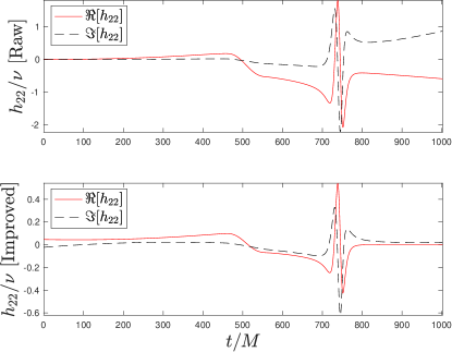
Figure 1: Obtaining the strain $h_{22}$ from $\psi^{4}_{22}$ using double integration in the time-domain, Eq. (3), demonstrated on the waveform from configuration $\#4$ of Table 2. Top panel: direct double integration in the time-domain, that highlights the presence of an unphysical global drift on both the real and imaginary parts. Bottom panel: improved waveform obtained removing a global straight line fitted to the data after each time-domain integration.

In this respect, it is worth mentioning that there is an especially delicate (and in fact dominant) source of uncertainty in the calculation of the angular momentum flux that we do not consider in our error bars. This comes from the recovery of the strain from the Weyl scalar $\psi_{4}$, a procedure that needs two time-integrations and thus the determination of two, arbitrary, integration constants. This turns out to be a complicated procedure for our simulations and we have investigated it briefly only for the $\ell=m=2$ mode. We use the following convention for the metric strain

$$h_{+}-ih_{\times}={\cal D}_{L}^{-1}\sum_{\ell=2}^{\rm\ell_{\rm max}}\sum_{\ell=-m}^{m}h_{\ell m}{}_{-2}Y_{\ell m}\ ,$$ (2)

where ${\cal D}_{L}$ is the luminosity distance and ${}_{-2}Y_{\ell m}$ are the $s=-2$ spin-weighted spherical harmonics. The usual relation between the strain modes and the $\psi^{4}$ modes is given by $\ddot{h}_{\ell m}={\cal D}_{L}\psi^{4}_{\ell m}$. The $\ell=m=2$ strain mode is thus obtained as

$$h_{22}=\int_{0}^{t}dt^{\prime}\int_{0}^{t^{\prime}}dt^{\prime\prime}{\cal D}_{L}\psi^{4}_{22}.$$ (3)

It is well known that the application of this formula on numerical waveforms extracted at finite radius may give unphysical features, with global drifts that might be nonlinear and difficult to subtract Berti et al. (2007). For quasi-circular binaries, performing the integration in the frequency domain typically gives a robust result Reisswig and Pollney (2011). The scattering, or hyperbolic encounter, setup doesn’t seem to have been explored so far in the literature. Notably Ref. Gold and Brügmann (2013) only explicitly shows $\psi^{4}_{\ell m}$ waveforms and did not attempt to compute the metric strain. Figure 1 refers to configuration $\#4$ of Table 2. The top panel of the figure shows the result of the direct integration of $\psi^{4}_{22}$: both the real and imaginary part of the waveform exhibit a quasi-linear, global, unphysical drift. Subtracting it by just removing a linear regression doesn’t seem to work. By contrast, in the bottom panel of the figure we show an improved waveform that is obtained by subtracting a global linear fit after each integration. The interval where the fit is performed is $[900,1000]$ for the real part and $[2,1000]$ for the imaginary part. Although the waveform looks qualitatively correct, the fact that the global quadratic behavior of the imaginary part is still indicating that some systematics is present. In general, this is not surprising since the main aim of our simulations was the computation of the angle from the puncture tracks, and not specifically the computation of the waveforms. It is likely that different grid setup, resolution, extraction radii could be useful to reduce the waveform uncertainties. Despite this, there are a few considerations that is still worth making using the current data. First, one notes that the waveform as a sort of bump around $t=400M$, that is prominent in the real part while it is absent in the imaginary part. That feature is related to the initial burst of junk radiation that is present in $\psi^{4}_{22}$ at approximately the same time. Second, as already mentioned above, differences in the strain will reflect on the computation of the losses $(\Delta J^{\rm NR},\Delta E^{\rm NR})$ listed in Tables 2-3. Focusing only on the (dominant) $\ell=m=2$ waveform mode we computed the losses using either the raw waveform, getting $(\Delta J^{\rm NR}_{22},\Delta E^{\rm NR}_{22})=(0.011571,0.12165)$, or the improved waveform, obtaining $(\Delta J^{\rm NR}_{22},\Delta E^{\rm NR}_{22})=(0.011566,0.11922)$. If the fractional difference for $\Delta E^{\rm NR}_{22}$ is negligible, for $(\Delta J^{\rm NR}_{22}$ we get a $2\%$, that might be even slightly larger because of the behavior of the precursor. In conclusion, our analysis shows that the calculation of $\Delta J^{\rm NR}$ could be overestimated by a few percents due to the double integration procedure. This specific analysis, as well as discussion of waveforms, is not within the scopes of this analysis and it is thus postponed to future work.

III EOB/NR comparisons

Reference Damour et al. (2014) pioneered the EOB/NR comparison of the scattering angle using several flavors of a (now outdated) EOB model. It is worth stressing that at the time a model incorporating radiation reaction along generic orbits was not available, so that it was possible instead to use the NR losses using a formula proposed in Ref. Bini and Damour (2012) that neglects quadratic effects in the radiation reaction and only relies on the knowledge of the EOB Hamiltonian. More recently, the progressive development of faithful EOB models valid for generic, non-quasi-circular, configurations Nagar et al. (2021a, b), and in particular the use of a consistent radiation reaction force, has revived the interest for scattering configurations so to test the model in an extreme regime. In particular, Ref. Nagar et al. (2021b) showed that an EOB model informed by quasi-circular NR simulations yields values of the scattering angle that are more consistent, also in strong field, with the NR computations of Ref. Damour et al. (2014). This EOB/NR agreement was improved further in Ref. Nagar and Rettegno (2021), that proposed an improved version of the TEOBResumS model for spin-aligned binaries on generic orbits crucially incorporating high-order (nonspinning) PN information Bini et al. (2019, 2020a, 2020b, 2020c) within the EOB potentials. In particular, Table V of Ref. Nagar and Rettegno (2021) reports what is currently the best agreement between EOB and NR scattering angles, with a fractional difference $\sim 3.8$ % for the most relativistic configuration computed numerically, reaching an EOB impact parameter $\sim 3.5$.

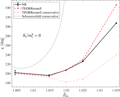
Figure 2: Scattering angle versus initial energy for the nonspinning systems of Table 2 for NR simulations (solid black curve) and TEOBResumS (dashed red line). We also plot the TEOBResumS scattering angle in the case of conservative motion (dashed pink curve) to show the impact of radiation reaction. The same is done for the case of a test particle moving around a Schwarzschild BH (grey line). Note that the the Schwarzschild line is computed using an initial angular momentum $p_{\varphi}^{\rm Schw}$ corresponding to the $\hat{J}^{\rm NR}_{\rm in,orb}$ to the first simulation of Table 2 ($\#1$). We can see that TEOBResumS is consistent with NR simulations for smaller energies but starts to deviate at higher ones.

For our current comparison we thus use the model of Ref. Nagar and Rettegno (2021). In order to ease the discussion, we do not report here any technical detail about the EOB construction, but directly refer the reader to Ref. Nagar and Rettegno (2021). As mentioned above, in order to assure a consistent match between EOB and NR simulations, the EOB dynamics is started with the NR energy and angular momentum $(\hat{E}^{\rm NR}_{in},\hat{J}^{\rm NR}_{\rm in,orb})$ calculated after the junk radiation, following precisely the scheme of Ref. Damour et al. (2014). We fix the EOB initial separation to $r_{0}=10000$; then, we identify $(\hat{E}^{\rm NR}_{in},\hat{J}^{\rm NR}_{\rm in,orb})$ with the initial EOB energy and angular momentum and out of this we determine the initial radial momentum $p_{r_{*}}$. From the evolution we compute the orbital phase $\varphi$ as function of time and we finally obtain $\chi^{\rm EOB}=\varphi-\pi$.

We focus first on the nonspinning configurations, that are reported in Table 2. For completeness, the data are also shown in Fig. 2. The model has an outstanding agreement with the simulated systems for smaller energies, which progressively worsens with the increase of the initial energy. This is to be expected, as high energies imply smaller impact parameters and hence strong-field interactions. We also show in Fig. 2 the scattering angle obtained using only the conservative sector of the EOB dynamics, setting to zero the radiation reaction force. The difference is noticeable, especially as the energy increases, which highlights the importance of the analytical radiation reaction in yielding consistent EOB/NR scattering angles. To orient the reader, we also report in Fig. 2 the scattering angle of a particle moving along the geodesics of the Schwarzschild metric. In this latter case, we identify $p_{\varphi}^{\rm Schw}=\hat{J}^{\rm NR}_{\rm in,orb}/\nu$ and $\hat{E}^{\rm Schw}=\hat{E}_{\rm eff,in}^{\rm NR}$, where the dimensionless effective energy is computed through the EOB relation

$$\hat{E}_{\rm eff}\equiv\frac{E^{2}-m_{1}^{2}-m_{2}^{2}}{2m_{1}m_{2}}.$$ (4)

Finally, we can visualize the energy regime we are exploring by looking at the initial circular Hamiltonians. We remind the reader that the real EOB Hamiltonian is obtained from the effective one through Eq. (4) and reads

$$H_{\rm EOB}=M\sqrt{1+2\nu\left(\hat{H}_{\rm eff}-1\right)}.$$ (5)

while the effective Hamiltonian (per unit of reduced mass) reads

$$\hat{H}_{\rm eff}\equiv\dfrac{H_{\rm eff}}{\mu}=\sqrt{p_{r_{*}}^{2}+A\left(1+p_{\varphi}^{2}u^{2})+Q\right)}\ ,$$ (6)

where $(A,Q)$ are the EOB potentials at 5PN (formal) accuracy as discussed in Ref. Nagar and Rettegno (2021). In the Schwarzschild limit, $Q=0$ and $A=1-2u$. In order to have a meaningful comparison, in Fig. 3 we show the Schwarzschild and TEOBResumS effective Hamiltonians together with the effective initial energies $\hat{E}_{\rm eff,in}^{\rm NR}$.

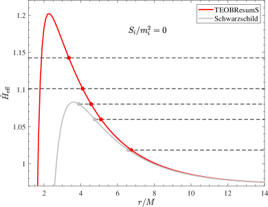
Figure 3: Comparison between the circular TEOBResumS effective Hamiltonian for equal-mass, nonspinning systems (red line) with its Schwarzschild equivalent (grey line). The angular momentum is set to the value of $\hat{J}^{\rm NR}_{\rm in,orb}$ of the first NR simulation of Table 2, so neglecting the (small) differences in initial angular momenta between the various configurations. The dotted horizontal lines correspond to the initial effective energies $\hat{E}_{\rm eff,in}^{\rm NR}$, computed from the $\hat{E}_{\rm in}^{\rm NR}$ of Table 2 using Eq. (4). We can see how these systems scatter within TEOBResumS, since the energies are all lower than the potential barrier, while this is not always the case for the Schwarzschild potential.

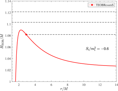
Figure 4: TEOBResumS circular Hamiltonian for equal-mass systems with large, anti-aligned spins ($S_{i}/m_{i}^{2}=-0.6$). The angular momentum is set to the value of $\hat{J}^{\rm NR}_{\rm in,orb}$ of the first NR simulation with the same spin in Table 3 ($\#s25$). The dotted horizontal lines correspond to the initial energies $\hat{E}_{\rm in}^{\rm NR}$ of the last 3 systems in Table 3. Here we note how two of the systems are plunging instead of scattering, because the potential barrier of TEOBResumS is too low.

Spinning configurations are listed in Table 3. One sees that the EOB/NR consistency is of the order of a few percents for the lowest energy configurations and for spins aligned with the orbital angular momentum. By contrast, when the spins are anti-aligned with the orbital angular momentum, the EOB/NR differences are rather large even for the smallest values of the energy. For large energies, while the NR simulations give a scattering, the corresponding EOB dynamics gives a plunge. The same also occurs for the spin-aligned case for the largest values of the energy. Phrasing this phenomenon in a different way, it seems that the EOB gravitational interaction is more attractive than what it is supposed to be. Not that although this is very evident for high energies, the global qualitative behavior is the same for all configurations, with the EOB angle always overestimating the NR prediction. This suggests that the strong-field behavior of the eccentric version of TEOBResumS, and possibly the spin sector of the model, should be improved in some way to better match these configurations. In practical terms, it is instructive to look at the EOB circular Hamiltonian for $S_{i}/m_{i}^{2}=-0.6$, Fig. 4. The three horizontal lines are the energies for the three configurations with the same spin values in Table 3. It is evident from this plot that to have a scattering for configurations $\#s26$ and $\#s27$ the EOB Hamiltonian should peak at a much higher value, yielding a larger potential barrier. The understanding of the modifications needed to the spin-sector of the current TEOBResumS eccentric model is postponed to future work. Let us only mention that it will be interesting to explore the performance of the new description of the spin-orbit sector proposed in the concluding section of Ref. Rettegno et al. (2019), that uses a different gauge choice to incorporate, in simple form, the Hamiltonian of a spinning particle derived in Ref. Barausse et al. (2009).

IV Conclusions

We have performed new numerical computations of the scattering angle $\chi$ of equal-mass BBH encounters. For the first time we have considered spinning BHs, with spins aligned or anti-aligned with the orbital angular momentum. This complements the 10, nonspinning, configurations simulated in Ref. Damour et al. (2014) with other 32 configurations, increasing the NR knowledge of the parameter space of scattering BBHs. Differently from the results of Ref. Damour et al. (2014), that were performed at fixed incoming energy, here we keep the initial angular momentum fixed while the incoming energy is varied. We find that the magnitude of the scattering angle increases with the incoming energy, analogously to the behavior of a test-particle scattering on a Kerr BH. The numerical results are compared with the predictions of the most developed version of the eccentric TEOBResumS model, introduced in Ref. Nagar and Rettegno (2021). For the nonspinning case, the new simulations further confirm the quality of the model also for scattering configurations, as already pointed out in Ref. Nagar and Rettegno (2021). The EOB/NR agreement is $\lesssim 1\%$ in all cases except for configuration $\#5$ of Table 2 where the EOB angle is larger than NR prediction by $\sim 13\%$. This indicates that the EOB dynamics should be improved further, notably by reducing the attractive character of the EOB potential $A$ [e.g. pushing the effective horizon at smaller values of $r$ by suitably tuning the effective 5PN parameter $a_{5}^{c}(\nu)$] so to consistently reduce the magnitude of the scattering angle. This result is a priori not surprising, since the potential $A$ was NR-informed only using quasi-circular NR simulations, i.e. in a rather different physical setup. Nonetheless, the $\simeq 13\%$ difference found in the most relativistic configuration actually indicates that the NR-tuning of $A$, as discussed in Ref. Nagar and Rettegno (2021), is robust and only partially dependent on the specific physical setup chosen to do it (in this case, quasi-circular configurations). By contrast, as far as spins are concerned the EOB/NR differences grow considerably, typically yielding scattering angles that are larger than the NR predictions. This indicates that the global attractive character of the EOB potentials (as obtained from the combined action of orbital and spin-orbital interactions) is too strong and should be weakened. How to do so in practice will hopefully be explored in future work.