Effective one-body model for extreme-mass-ratio spinning binaries on eccentric equatorial orbits: testing radiation reaction and waveform

Abstract

We provide a systematic analysis of the multipolar gravitational waveform, energy and angular momentum fluxes emitted by a nonspinning test particle orbiting a Kerr black hole along equatorial, eccentric orbits. These quantities are computed by solving numerically the Teukolsky equation in the time domain using Teukode and are then used to establish the reliability of a recently introduced prescription to deal with eccentricity-driven effects in the radiation reaction (and waveform) of the effective-one-body (EOB) model. The prescription relies on the idea of incorporating these effects by replacing the quasi-circular Newtonian (or leading-order) prefactors in the EOB-factorized multipolar waveform (and fluxes) with their generic counterparts. To reliably account for strong-field regimes, standard factorization and resummation procedures had to be implemented also for the circular sector of $\ell=7$ and $\ell=8$ waveform multipoles. The comparison between numerical and analytical quantities is carried out over a large portion of the parameter space, notably for orbits close to the separatrix and with high eccentricities. The analytical fluxes agree to $\sim 2\%$ with the numerical data for orbits with moderate eccentricities($e\lesssim 0.3$) and moderate spins (${\hat{a}}\lesssim 0.5$), although this increases up to $\sim 33\%$ for large, positive, black hole spins ($\sim 0.9$) and large eccentricities ($\sim 0.9$). Similar agreement is also found for the waveform. For moderate eccentricities, the EOB fluxes can be used to drive the test-particle dynamics through the nonadiabatic transition from eccentric inspiral to plunge, merger and ringdown. Over this dynamics, we construct a complete EOB waveform, including merger and ringdown, that shows an excellent phasing and amplitude agreement with the numerical one. We also show that the same technique can be applied to hyperbolic encounters. In general, our approach to radiation reaction for eccentric inspirals should be seen as a first step toward EOB modelization of extreme-mass-ratio-inspirals waveforms for LISA.

I Introduction

The gravitational waves (GWs) observed by LIGO and Virgo Acernese et al. (2015); Aasi et al. (2015) are generated by the last stages of the coalescence of compact binary systems with comparable masses Abbott et al. (2021). These systems lose energy and angular momentum due to GW emission, that causes the progressive circularization of the orbit. Therefore, most of the current gravitational wave templates used for the analysis of the signals adopt the quasi-circular approximation. Nonetheless, dynamical captures are possible in dense environments, such as active galactic nuclei and globular clusters, leading to the formation of binaries with nonvanishing eccentricity, as shown in recent population studies Mukherjee et al. (2020); Romero-Shaw et al. (2019). The dynamical capture scenario is also relevant for the analysis of GW190521 Abbott et al. (2020); Romero-Shaw et al. (2020). Other systems where the eccentricity plays a key role are Extreme Mass Ratio Inspirals (EMRIs), binaries where a compact stellar object orbits around a supermassive black hole. Gravitational waves from EMRIs have characteristic frequencies around the mHz, making them one of the most relevant sources for the Laser Interferometer Space Antenna (LISA) Amaro-Seoane (2018). For these reasons, the inclusion of eccentricity in the current theoretical waveform models has drawn interest in the last few years, leading to the realization of many models for bound configurations with, in general, relatively mild eccentricity, such as ENIGMA Huerta et al. (2018), SEOBNRE  Cao and Han (2017); Liu et al. (2019, 2021), NRSur2dq1Ecc Islam et al. (2021), TEOBResumS Chiaramello and Nagar (2020); Nagar et al. (2021a, b) and Refs. Tanay et al. (2016); Moore and Yunes (2019); Boetzel et al. (2019); Tiwari et al. (2019); Tiwari and Gopakumar (2020).

The effective one body approach (EOB) currently represents the most complete, reliable and predictive analytical framework able to deal with inspiraling and coalescing relativistic binaries. By design, the EOB approach is superior to standard post-Newtonian techniques because it structurally incorporates nonperturbative elements (e.g., the existence of a last stable orbit) that allow for a robust computation of observable quantities, like waveforms and fluxes, also in strong field, i.e. even beyond the last stable orbit up to merger. The synergy between the EOB approach and Numerical Relativity (NR) simulations proved highly successful to provide highly accurate waveform templates for coalescing BBHs and BNS as observed by LIGO and Virgo. By contrast, systems with large mass ratios like EMRIs cannot be explored using NR techniques, while they are naturally described within the EOB approach. In addition: (i) the extreme mass ratio limit plays a pivotal role in the EOB development, especially for what concerns waveforms and fluxes, that can be informed/compared with numerical results  Nagar et al. (2007); Damour and Nagar (2007); Bernuzzi and Nagar (2010); Bernuzzi et al. (2011a, b, 2012); Harms et al. (2014); Nagar et al. (2014); Harms et al. (2016a, b); Lukes-Gerakopoulos et al. (2017); Nagar et al. (2019a), and (ii) a fairly large amount of work has been dedicated to calculate analytically gravitational self-force terms and provide comparisons with numerical results Damour (2010); Barack et al. (2010); Akcay et al. (2012); Bini and Damour (2014, 2015); Akcay and van de Meent (2016); Barack et al. (2019).

The EOB relativistic dynamics relies on three building blocks: (i) a Hamiltonian; (ii) a prescription for computing the radiation reaction; (iii) a prescription for computing the waveform. Typically, points (ii) and (iii) are interconnected, because the radiation reaction, i.e. the gravitational wave fluxes of energy and angular momentum, are obtained by summing together resummed waveform multipoles. In this respect, Ref. Chiaramello and Nagar (2020) proposed to incorporate noncircular effects in radiation reaction (and waveform) replacing the quasi-circular Newtonian (pre)factors with their generic counterparts. Recently Nagar et al. (2021b), improvement of this approach allowed to build an EOB eccentric waveform model that is highly faithful with the (tiny) number of eccentric NR simulations publicly available. Nonetheless, a systematic understanding and checking of this Newtonian-improved quantities is missing, despite the preliminary results shown in Ref. Chiaramello and Nagar (2020). Historically, the systems made by a small black hole of mass $\mu$ orbiting a large black hole with mass $M$ such that $\nu\equiv\mu/M\ll 1$ proved a useful laboratory to test and verify ideas or methods within the EOB approach before adopting them in the comparable-mass case Damour et al. (2009). This practice was in particular followed in Ref. Chiaramello and Nagar (2020), that highlighted the excellent agreement between analytical and numerical waveform and fluxes in the test-mass case (see Fig. 1 therein, limited to geodesic motion with $e=0.3$). The purpose of this paper is to systematically extend the analysis of Chiaramello and Nagar (2020) up to large values of the eccentricity, also including the black hole spin. We will thus mainly focus on analytical/numerical flux comparisons of extreme mass ratio binaries: a test-mass object orbits around a Kerr black hole along eccentric equatorial geodesics. The comparisons of the analytical fluxes with the numerical ones obtained from the time-domain (TD) code Teukode Harms et al. (2014) will provide a reliability-test of the radiation reaction. We will also test the reliability of the analytical prescription for the waveform. Our model should be intended as a first step toward the modelization of EMRIs within the EOB framework. An physically more faithful description of EMRIs will certainly need to include high-order noncircular terms beyond the leading order in the radiation reaction as well as results from Gravitational Self-Force theory within the EOB Hamiltonian (i.e., linear in the mass ratio $\nu$ beyond the geodesic dynamics Barack and Pound (2019)). This aim goes beyond the purpose of the present work. As a consequence, most of the work presented in this paper should be considered as an exploratory investigation that will be refined further in the future. In particular, we shall consider an analytical/numerical agreement for instantaneous eccentric fluxes to be good if the fractional differences are around or below the few percents, indicatively $\lesssim 5\%$. For the corresponding averaged fluxes, we expect smaller differences. For what concerns eccentric waveforms, we aim at reaching numerical/analytical fractional differences of a few percents in the amplitude and of a few hundredth of a radian in the phase difference. We will show that this accuracy, considered good within our context, is achieved in a large portion of the parameter space.

The paper is structured as follows. In Sec. II we expose the Hamiltonian formalism used to describe the dynamics of a test-particle around a Kerr black hole and the numerical methods used to perform the simulations. In Sec. III, after a brief introduction of the EOB model, we describe the analytical waveform and fluxes in details and the new improvements introduced to the circular Post-Newtonian (PN) factors. In Sec. IV, we study the phenomenology of the fluxes and we compare the numerical and analytical fluxes to establish the reliability of the radiation reaction. In Sec. V we provide a comparison between numerical and analytical waveforms, also showing the full transition from an eccentric inspiral to plunge, merger and ringdown, as well as waveforms from dynamical captures.

Through this paper, we will use geometrized units $G=c=1$. Moreover, the time and the phase-space variables used in this work are related to the physical ones by $t=T/(GM)$, $r=R/(GM)$, $p_{r}=P_{R}/\mu$ and $p_{\varphi}=P_{\varphi}/(\mu GM)$.

II Numerical waveforms and fluxes

II.1 Equatorial dynamics around a Kerr black hole

For a test-particle orbiting in the equatorial plane of a Kerr black hole of dimensionless spin ${\hat{a}}\equiv J_{\rm BH}/M^{2}$ the EOB Hamilton’s equations for spin-aligned objects reduce to Damour and Nagar (2014a); Harms et al. (2016b)

$$\dot{r} =\left(\frac{A}{B}\right)^{1/2}\frac{\partial{\hat{H}^{\rm eq}_{\rm Kerr}}}{\partial p_{r_{*}}},$$ (1)

$$\dot{\varphi} =\frac{\partial{\hat{H}^{\rm eq}_{\rm Kerr}}}{\partial p_{\varphi}}\equiv\Omega,$$ (2)

$$\dot{p}_{r_{*}} =\left(\frac{A}{B}\right)^{1/2}\left(\hat{{\cal F}}_{r}-\frac{\partial{\hat{H}^{\rm eq}_{\rm Kerr}}}{\partial r}\right),$$ (3)

$$\dot{p}_{\varphi} =\hat{{\cal F}}_{\varphi}.$$ (4)

Here, $\hat{{\cal F}}_{r,\varphi}\equiv{\cal F}_{r,\varphi}/\nu$ are the radial and angular components of the radiation reaction force and ${\hat{H}^{\rm eq}_{\rm Kerr}}$ is the $\mu$-normalized test-particle Hamiltonian Damour and Nagar (2014a), that reads

$${\hat{H}^{\rm eq}_{\rm Kerr}}=\frac{2{\hat{a}}p_{\varphi}}{rr_{c}^{2}}+\sqrt{A\mathinner{\left(r\right)}\mathinner{\left(1+\frac{p_{\varphi}^{2}}{r_{c}^{2}}\right)}+p_{r_{*}}^{2}}.$$ (5)

The metric functions $A(r)$ and $B(r)$ read

$$A(r) =\frac{1+2u_{c}}{1+2u}\left(1-2u_{c}\right)\ ,$$ (6)

$$B(r) =\frac{1}{1-2u+{\hat{a}}^{2}u^{2}}\ ,$$ (7)

where $u=1/r$, $u_{c}=1/r_{c}$, and $r_{c}$ is the centrifugal radius defined as Damour and Nagar (2014a)

$$r_{c}^{2}=r^{2}+{\hat{a}}^{2}+2\frac{{\hat{a}}^{2}}{r}.$$ (8)

Finally, $p_{r_{*}}$ is the conjugate momentum of the tortoise coordinate $r_{*}$, defined as $p_{r_{*}}=\sqrt{A/B}\;p_{r}$. Being planar, the orbit is fully determined by the choice of the eccentricity $e$ and the semilatus rectum $p$. Although it is not possible to provide a gauge invariant definition of $(e,p)$, in the test-particle limit it is natural to define them in analogy with Newtonian mechanics. For bound orbits, we have

$$e=\frac{r_{+}-r_{-}}{r_{+}+r_{-}},\quad\quad p=\frac{2r_{+}r_{-}}{r_{+}+r_{-}},$$ (9)

where $r_{\pm}$ are the two radial turning points, i.e. the apastron, $r_{+}$, and the periastron, $r_{-}$. Using the definitions of eccentricity and semilatus rectum, one finds $r_{\pm}=p/(1\mp e)$. In order to obtain a link between $(e,p)$ and the energy and angular momentum $(\hat{E},p_{\varphi})$, we analytically solve the two-equations system obtained by considering

$$\hat{E}={\hat{H}^{\rm eq}_{\rm Kerr}}|_{p_{r_{*}}=0}=\frac{2{\hat{a}}p_{\varphi}}{rr_{c}^{2}}+\sqrt{A\mathinner{\left(r\right)}\mathinner{\left(1+\frac{p_{\varphi}^{2}}{r_{c}^{2}}\right)}}$$ (10)

evaluated at the two radial turning points $r_{\pm}$, where $p_{r_{*}}=0$ by definition. Then for each pair of initial eccentricity and semilatus rectum $(e_{0},p_{0})$, we obtain the initial energy and angular momentum $(\hat{E}_{0},p_{\varphi}^{0})$. Finally, using the convention that the (cyclic) azimuthal variable $\varphi$ is set to zero at apastron, we have all the initial values needed to compute the evolution of the system through Hamilton’s equations. For geodesic motion, i.e. when $\hat{{\cal F}}_{\varphi}=\hat{{\cal F}}_{r}=0$, the eccentricity and the semilatus rectum (or, equivalently, $\hat{E}$ and $p_{\varphi}$) are constants of motion.

It is important to consider that for a given Kerr background, not all the eccentricity-semilatus rectum pairs produce stable orbits. In fact, in order to have a bound orbits, the Kerr potential (Eq.(2) of O’Shaughnessy (2003)) must have three roots: $(\bar{r},r_{-},r_{+})$. When $r_{-}=\bar{r}$, the bound motion is only marginally allowed, and when the potential has only two roots the particle inevitably plunges toward the event horizon. Therefore, for stable bound orbits we must have $p>p_{s}$, where $p_{s}$ is known as separatrix and depends both on eccentricity and spin. The separatrix can be found as a root of O’Shaughnessy (2003); Stein and Warburton (2020)

$$p_{s}^{2}(p_{s}-6-2e)^{2}+{\hat{a}}^{4}(e-3)^{2}(e+1)^{2}$$ (11)

$$-2{\hat{a}}^{2}(1+e)p_{s}\left[14+2e^{2}+p_{s}(3-e)\right]=0.$$

Note that in the Schwarzchild case, the separatrix is simply given by $p_{s}=6+2e$.

II.2 Waveform and fluxes

From the particle dynamics, we compute waveforms and fluxes at leading order in the mass ratio $\nu$. This is done either numerically, solving the Teukolsky or Regge-Wheeler-Zerilli (RWZ) perturbation equations Regge and Wheeler (1957); Zerilli (1970), or analytically, using suitable resummations of post-Newtonian results as discussed in Sec. III below. To fix conventions, let us remind that the waveform is decomposed in multipoles $h_{\ell m}$ as

$$h_{+}-{\rm i}h_{\times}=D_{L}^{-1}\sum_{{\ell}=2}^{{\ell}_{\rm max}}\sum_{m=-{\ell}}^{{\ell}}h_{\ell m}\,{}_{-2}Y_{\ell m},$$ (12)

where $D_{L}$ is the luminosity distance and ${}_{-2}Y_{\ell m}$ are the spin-weighted spherical harmonics with weight $s=-2$. We will often work with the RWZ-normalized waveform Nagar and Rezzolla (2005) $\Psi_{{\ell m}}=h_{{\ell m}}/\sqrt{(\ell+2)(\ell+1)\ell(\ell-1)}$. The energy and angular momentum fluxes at future null-infinity, $\dot{E}$ and $\dot{J}$, can be computed from the multipolar waveform as

$$\dot{E} =\;\;\,\frac{1}{16\pi}\sum_{{\ell}=2}^{\ell_{\rm max}}\sum_{m=-{\ell}}^{{\ell}}|\dot{h}_{{\ell m}}|^{2},$$ (13a)

$$\dot{J} =-\frac{1}{16\pi}\sum_{{\ell}=2}^{\ell_{\rm max}}\sum_{m=-{\ell}}^{{\ell}}m\Im\left(\dot{h}_{{\ell m}}h_{{\ell m}}^{*}\right)\ .$$ (13b)

We will fix $\ell_{\rm max}=8$, since the contributions of the higher ones is negligible. In fact, even the $\ell=8$ modes have typically contributions $\lesssim 1\%$, and only in some very strong-field regimes their contribution can reach the $2\%$. For example, we anticipate that for $({\hat{a}},e,p)=(0.9,0.9,p_{s}+0.01)$, we get a relative contribution to $\dot{J}$ of $2.2\%$ (the (8,8) mode alone contributes to $2.1\%$). The contribution of the subdominant modes to the fluxes will be discussed in more detail in Sec. IV.3.

II.3 Numerical methods and setup

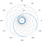
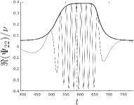
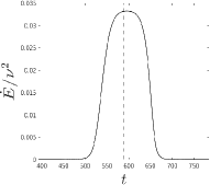
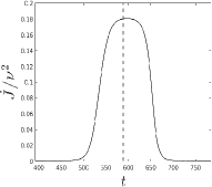
Figure 1: Top panels: a complete radial orbit of the simulation with ${\hat{a}}=0.6$, $e=0.7$ and $p=p_{s}+0.01\simeq 4.858$ and the corresponding real part of the dominant mode of the numerical waveform. The dashed vertical line marks the periastron passage. Bottom panels: energy and angular momentum fluxes summed up to ${\ell}_{\rm max}=8$. Note the zoom-whirl behavior and the periastron precession. Moreover, it is possible to observe the fluxes (and waveform) asymmetry that we will discuss in Sec. IV.

To apply black-hole perturbation theory to our waveform (and flux) calculation, we solve, in the time-domain, the Regge-Wheeler-Zerilli (RWZ) Regge and Wheeler (1957); Zerilli (1970) or Teukolsky equations in the presence of a point-particle source, that is represented by a $\delta$-function. Following a practice introduced long ago Nagar et al. (2004, 2007), the $\delta$-function is approximated by a narrow Gaussian function. In the Schwarzschild background case, we solve the RWZ equations in the time-domain using the RWZhyp code developed long ago Bernuzzi and Nagar (2010); Bernuzzi et al. (2012), that notably employs the hyperboloidal layer method Bernuzzi et al. (2011b) to extract the waveforms at future null infinity, avoiding errors related to the wave extraction at finite radius. In the more general case of a rotating black hole, we use Teukode Harms et al. (2014) to solve the Teukolsky equation in the time-domain. In particular, the code uses horizon-penetrating and hyperboloidal coordinates that allow for the inclusion of the horizon and the future null infinity in the computational domain Zenginoğlu (2008); Zenginoğlu and Tiglio (2009); Zenginoğlu (2011). The 3+1 equation is decomposed exploiting the axisimmetry of the Kerr spacetime obtaining a 2+1 TD equation for each Fourier $m$-mode in the azimuthal direction. Then the wave equation is solved for gravitational perturbations, obtaining the Weyl scalar $\Psi_{4}$, i.e. the contraction of the Weyl scalar with a null-tetrad (the Hawking-Hartle tetrad in our case). Each waveform multipole is then obtained by a double time integration of the Weyl scalar, since at infinity $\ddot{h}_{\ell m}=\Psi_{4}^{\ell m}$, where $\Psi_{4}^{\ell m}$ is the multipolar decomposition of $\Psi_{4}$. Analogously to the RWZhyp code, the formal Dirac $\delta$ functions present in the source term are approximated using narrow Gaussian functions. In our simulations, we use horizon-penetrating, hyperboloidal coordinates with scri-fixing at $S=10$ and resolution of $N_{r}\times N_{\theta}=3600\times 160$, where $(N_{r},N_{\theta})$ are the number of points in the radial and angular directions respectively. From the Hamiltonian dynamics for the particle discussed in Sec. II.1, we compute the waveforms and the fluxes at infinity using the two numerical codes exposed above. Teukode is more general than RWZhyp, but the computational time is also greater. Nonetheless, we will use Teukode also for nonspinning cases, with the only exception of few simulations with large semilatera recta ($p=21,31$). We will explicitly state when results from RWZhyp are presented; otherwise, Teukode is understood. An example of (zoom-whirl) geodesics dynamics (${\cal F}_{r}={\cal F}_{\varphi}=0$) with the corresponding $\ell=m=2$ waveform multipole and fluxes is shown in Fig. 1.

II.4 Comparisons with previous work

Table 1: Averaged numerical fluxes computed with RWZhyp and Teukode compared with results present in the literature, see discussion in the text.

		Teukode (TD)	Teukode (TD)	RWZhyp (TD)	Martel (TD)	Barack (GSF)	Fujita (FD)
		$3600\times 160$	$5400\times 320$
$p=7.50478$	${\langle\dot{E}\rangle}\cdot 10^{4}$	3.16885	3.16888	3.17077	$3.1770$	$3.1691$	$3.16899989184$
$e=0.188917$	${\langle\dot{J}\rangle}\cdot 10^{3}$	5.96731	5.96737	5.96998	$5.9329$	$5.967608$	$5.96755215608$
$p=8.75455$	${\langle\dot{E}\rangle}\cdot 10^{4}$	2.12276	2.12269	2.12718	$2.1484$	$2.1243$	$2.12360313326$
$e=0.764124$	${\langle\dot{J}\rangle}\cdot 10^{3}$	2.77643	2.77635	2.78077	$2.7932$	$2.77746$	$2.77735938996$

Both RWZhyp and Teukode have never been used systematically for eccentric runs before (see however Ref. Chiaramello and Nagar (2020)), therefore we need to test the consistency of our results with published results. To do so, we compare the averaged fluxes along a radial orbit for both Schwarzschild and Kerr backgrounds.

For the nonspinning case, the comparisons are shown in Table 1, where our $\nu$-normalized fluxes averaged over a radial period (see Eq. (38) below) are compared with the classic TD results of Martel Martel (2004), as well as to more recent Gravitation-Self-Force (GSF) calculations of Barack and Sago Barack and Sago (2010) and FD results of Fujita Fujita et al. (2009). Note that we sum the multipoles up to $\ell_{\rm max}=8$, but in the other works $\ell_{\rm max}$ assumes different values. Despite these differences, the agreement with previous computations remains satisfactory, since the higher multipoles are highly subdominants. We can also observe that among the TD codes, Teukode is the most accurate one. Note that the difference between resolutions $3600\times 120$ and $5400\times 320$ is very small. Since in the second case the computational time increases by a factor 6, we will use the former resolution. We have also compared the instantaneous energy and angular momentum fluxes of Teukode and RWZhyp in the cases $(e,p)=(0.3,9),(0.5,11)$, $(0.8,13)$, and we have seen that the relative difference between the two numerical fluxes reaches its maximum at periastron and it is at most of $0.3\%$.

In the presence of black hole spin, we have compared the averaged fluxes for ${\hat{a}}=0.5$ and $e=0.5$ obtained using Teukode with the results of Glampedakis and Kennefick Glampedakis and Kennefick (2002). The comparison, shown in Table 2, highlights the good agreement, with discrepancies below $0.2\%$. Note however that, as above, we fixed ${\ell}_{\rm max}=8$, while Ref. Glampedakis and Kennefick (2002) sums up to ${\ell}_{\rm max}=10-17$ and this affects the comparison. In fact, in the first case reported in Table 2, the ${\ell}=8$ modes have a relative contribution of $\sim 0.25\%$ to the total fluxes, therefore including also the multipoles with ${\ell}>8$ would probably improve the agreement. Note also that when the semilatus rectum is increased, the agreement improves, because the higher modes become less and less relevant. We have also considered a configuration with ${\hat{a}}=0.9$, $e\simeq 0.3731$ and $p\simeq 12.152$, calculated both in Ref. Shibata (1994) and Ref. Glampedakis and Kennefick (2002). In this case, the contribution of the ${\ell}=8$ modes is only of the order of $2\cdot 10^{-5}$ due to the large value of $p$ used, and as a consequence the discrepancy is smaller. Nonetheless, comparing the energy and angular momentum fluxes with the results of Ref. Shibata (1994), we have found, respectively, discrepancies of $1.4\%$ and of $0.8\%$, confirming the $\sim 1\%$ disagreement already found by Ref. Glampedakis and Kennefick (2002). We can thus conclude that our numerical computations of the fluxes along eccentric orbits are consistent with all results already present in the literature. Our numerical approach is then expected to faithfully describe fluxes from eccentric orbits both on Schwarzschild and Kerr spacetimes.

Table 2: Numerical averaged fluxes in Kerr spacetime. We compare the results of Teukode (${\ell}_{\rm max}=8$) with the results obtained by Ref. Glampedakis and Kennefick (2002) (${\ell}_{\rm max}=10-17$). For the last simulation, only ${\langle\dot{E}_{GK}\rangle}$ is reported in Ref. Glampedakis and Kennefick (2002).

${\hat{a}}$	$e$	$p$	${\langle{\dot{E}_{\rm teuk}}\rangle}$	${\langle{\dot{J}_{\rm teuk}}\rangle}$	${\langle\dot{E}_{GK}\rangle}$	${\langle\dot{J}_{GK}\rangle}$
			$\cdot 10^{3}$	$\cdot 10^{2}$	$\cdot 10^{3}$	$\cdot 10^{2}$
0.5	0.5	5.1	4.20753	3.25791	4.21594	3.26383
0.5	0.5	5.5	2.11538	1.89340	2.11797	1.89546
0.5	0.5	6.0	1.19519	1.22870	1.19638	1.22973
0.9	0.3731	12.152	0.023571	0.080743	0.023570	/

II.5 Numerical geodesic simulations

In order to meaningfully cover the parameter space, we run 144 geodesic simulations with Teukode choosing eccentricities $e=(0,0.1,0.3,$ $0.5,0.7,0.9)$ and spins in the range ${\hat{a}}\in[-0.9,0.9]$, typically ${\hat{a}}=(0,\pm 0.2,\pm 0.6,\pm 0.9)$. For each pair of spin and eccentricity $({\hat{a}},e)$, we have chosen three different semilatera recta. The first is $p=p_{s}+0.01$, where $p_{s}=p_{s}(e,{\hat{a}})$ is the separatrix, while the other two are selected according to $p=p_{\rm schw}p_{s}(e,{\hat{a}})/p_{s}(e,0)$, where $p_{\rm schw}$ is 9 or 13. Depending on the value of the semilatus rectum, we will refer to the simulations, respectively, as near, intermediate and distant. The near simulations exhibit a zoom-whirl behavior, while the others generally have eccentric orbits without whirls at periastron. The complete list of the Teukode geodesic simulations with the corresponding averaged fluxes can be found in Appendix D. Hereafter, when we will report a semilatus rectum or a separatrix, we will truncate it to the third decimal.

III Analytical waveforms and fluxes

III.1 Waveform

Let us turn now to the discussion of the factorized and resummed analytical waveforms and fluxes along eccentric orbits. The basic ideas are those introduced in Ref. Damour et al. (2009) for the circular case, that proposed a recipe to factorize and resum the PN-expanded waveform multipoles. A simple procedure to generalize it to the case of eccentric orbits was introduced in Ref. Chiaramello and Nagar (2020), that we review here in detail. Each waveform multipole is factorized as

$$h_{{\ell m}}=h_{{\ell m}}^{(N,\epsilon)}\hat{h}^{(\epsilon)}_{{\ell m}}=h_{{\ell m}}^{(N,\epsilon)}\hat{S}^{(\epsilon)}\hat{h}_{\ell m}^{\rm tail}(\rho_{{\ell m}})^{{\ell}},$$ (14)

where $\epsilon$ denotes the parity of the multipole ($\epsilon=0$ if ${\ell}+m$ is even, $\epsilon=1$ if ${\ell}+m$ is odd), $h_{{\ell m}}^{(N,\epsilon)}$ is the Newtonian contribution and $\hat{h}^{(\epsilon)}_{{\ell m}}$ is the PN correction. The term $\hat{S}^{(\epsilon)}$ is the effective-source term, i.e. the energy if $\epsilon=0$ or the Newton-normalized angular momentum if $\epsilon=1$; $\hat{h}_{\ell m}^{\rm tail}=T_{{\ell m}}e^{i\delta_{{\ell m}}}$ is the tail factor and the $\rho_{{\ell m}}$ are the residual amplitude corrections. While the $S^{(\epsilon)}$ is general because it is computed along the general dynamics, the functions $\hat{h}_{\ell m}^{\rm tail}$ and $\rho_{\ell m}$ correspond to those obtained in the circular case (see Appendix A for more details). Following Ref. Chiaramello and Nagar (2020), the multipolar waveform is generalized to generic orbits (including open orbits Nagar et al. (2021a, b)) by simply replacing the Newtonian quasi-circular prefactor with its general expression. We remark that we are considering the waveform at leading order in $\nu$, therefore we switch off all the subleading $\nu$-dependencies in the factors of Eq. (14), except for the leading Newtonian contribution $O(\nu)$.

The Newtonian contribution of the waveform is obtained from the derivatives of the source multipoles, explicitly

$$h_{{\ell m}}^{(N,\epsilon)}\propto\begin{cases}I_{{\ell m}}^{({\ell})}&{\rm if}\;\;\;\epsilon=0\\ S_{{\ell m}}^{({\ell})}&{\rm if}\;\;\;\epsilon=1\\ \end{cases},$$ (15)

where $I_{{\ell m}}^{({\ell})}$ and $S_{{\ell m}}^{({\ell})}$ are the ${\ell}$th-derivatives of the mass and current source multipoles. For a test-particle orbiting in the equatorial plane of a Kerr black hole, they are given by

$$\begin{split}I_{{\ell m}}&\propto\nu r^{{\ell}}e^{-im\varphi},\\ S_{{\ell m}}&\propto\nu r^{{\ell}+1}\Omega e^{-im\varphi}.\end{split}$$ (16)

For circularized binaries, the derivatives of the radius and the orbital frequency are zero, but in the more general case they are not vanishing. Therefore the waveform can be generalized Chiaramello and Nagar (2020) (at Newtonian level) without neglecting the derivatives of the radius and of the orbital frequency, obtaining a general Newtonian contribution $h_{{\ell m}}^{(N,\epsilon)_{\rm tot}}$ that can be separated in circular and noncircular factors, respectively $h_{\ell m}^{(N,\epsilon)_{c}}$ and $h_{\ell m}^{(N,\epsilon)_{nc}}$. Then the full multipolar waveform can be written as

$$h_{{\ell m}}=h_{{\ell m}}^{(N,\epsilon)_{\rm c}}\hat{h}_{{\ell m}}^{(N,\epsilon)_{\rm nc}}\hat{h}^{(\epsilon)}_{{\ell m}},$$ (17)

where

$$\hat{h}_{{\ell m}}^{(N,0)_{\rm nc}} =\left(h_{{\ell m}}^{(N,0)_{\rm c}}\right)^{-1}I_{{\ell m}}^{({\ell})},$$

$$\hat{h}_{{\ell m}}^{(N,1)_{\rm nc}} =\left(h_{{\ell m}}^{(N,1)_{\rm c}}\right)^{-1}S_{{\ell m}}^{({\ell})},$$

$$h_{{\ell m}}^{(N,\epsilon)_{\rm c}}\;\, =h_{{\ell m}}^{(N,\epsilon)_{\rm tot}}(r,\Omega,\dot{r}=0,\dot{\Omega}=0,...).$$

For the dominant $(2,2)$ mode, the Newtonian noncircular correction reads

$$\hat{h}_{22}^{(N,0)_{\rm nc}}=1-\frac{\ddot{r}}{2r\Omega^{2}}-\frac{\dot{r}^{2}}{2r^{2}\Omega^{2}}+\frac{2\mathrm{i}\dot{r}}{r\Omega}+\frac{\mathrm{i}\dot{\Omega}}{2\Omega^{2}}.$$ (18)

The explicit noncircular corrections for the most relevant subdominant modes can be found in Appendix B.

III.2 Energy and angular momentum fluxes

The radiation reaction forces $({\cal F}_{\varphi},{\cal F}_{r})$ are obtained requiring the equality between the loss of mechanical energy and angular momentum of the system and the energy and angular momentum fluxes carried by the GW at infinity, $\dot{E}$ and $\dot{J}$. Using the angular and radial components of the radiation reaction and the equations of motion, the balance equations read Bini and Damour (2012)

$$\dot{r}{\cal F}_{r}+\Omega{\cal F}_{\varphi}+\dot{E}_{\rm Schott}+\dot{E}=0,$$ (19a)

$${\cal F}_{\varphi}+\dot{J}=0.$$ (19b)

where $\dot{E}_{\rm Schott}$ is the time-derivative of the Schott energy, that represents the interaction of the source with the local field and its orbital average goes to zero. The Schott contribution to the angular momentum, $\dot{J}_{\rm Schott}$, can be gauged away Bini and Damour (2012). In the circular case, ${\cal F}_{r}$ and $\dot{E}_{\rm Schott}$ vanish and we only have the angular component of the radiation reaction, that is typically written as

$$\hat{{\cal F}}_{\varphi}=-\frac{32}{5}\nu r_{\Omega}^{4}\Omega^{5}\hat{f},$$ (20)

where $\hat{f}$ is Newton-normalized flux function, that incorporates all the resummed PN corrections, and

$$r_{\Omega}=r\left(1+{\hat{a}}r^{-3/2}\right)^{2/3}.$$ (21)

The form of $\hat{f}$ is reminded in Appendix A. We recall that the analytic expression we use here relies on several previous works Damour et al. (2009); Nagar and Shah (2016); Messina et al. (2018) and, in particular, it uses resummed multipoles up to $\ell=8$. In Ref. Chiaramello and Nagar (2020), it was proposed to include noncircular effects in the angular component of the radiation reaction by means of the leading, quadrupolar, noncircular factor ${{\hat{f}_{\varphi,22}^{\rm N_{nc}}}}$,

$$\hat{{\cal F}}_{\varphi}=-\frac{32}{5}\nu r_{\Omega}^{4}\Omega^{5}{{\hat{f}_{\varphi,22}^{\rm N_{nc}}}}\hat{f}\equiv{\hat{{\cal F}}_{\varphi}^{\rm old}},\\$$ (22)

that reads

$${\hat{f}_{\varphi,22}^{\rm N_{nc}}}=1 +\frac{3\dot{r}^{4}}{4r^{4}\Omega^{4}}+\frac{3\dot{r}^{3}{\dot{\Omega}}}{4r^{3}\Omega^{5}}+\frac{3\ddot{r}^{2}}{4r^{2}\Omega^{4}}+\frac{3\ddot{r}\dot{r}{\dot{\Omega}}}{8r^{2}\Omega^{5}}$$

$$-\frac{{r^{(3)}}\dot{r}}{2r^{2}\Omega^{4}}+\frac{\dot{r}^{2}{\ddot{\Omega}}}{8r^{2}\Omega^{5}}+\frac{4\dot{r}^{2}}{r^{2}\Omega^{2}}+\frac{\ddot{r}{\ddot{\Omega}}}{8r\Omega^{5}}$$

$$-\frac{2\ddot{r}}{r\Omega^{2}}-\frac{{r^{(3)}}{\dot{\Omega}}}{8r\Omega^{5}}+\frac{3\dot{r}{\dot{\Omega}}}{r\Omega^{3}}+\frac{3{\dot{\Omega}}^{2}}{4\Omega^{4}}-\frac{{\ddot{\Omega}}}{4\Omega^{3}}.$$ (23)

This factor is simply the next-to-quasi-circular part of the Newtonian contribution to the angular momentum flux obtained from the Newtonian quadrupolar waveform $h_{22}^{(N,0)}$. More precisely, one has

$$\dot{J}^{\rm N}_{22}/\nu\equiv-\dfrac{1}{8\pi}\sum_{m=\pm 2}\Im\left(\dot{h}_{2m}^{(N,0)}h_{2m}^{(N,0)*}\right)=\dfrac{32}{5}\nu r^{4}\Omega^{5}{{\hat{f}_{\varphi,22}^{\rm N_{nc}}}},$$ (24)

that, after replacing $r$ with $r_{\Omega}$, changing sign, and considering $\hat{f}$, finally yields Eq. (22). Although this choice was used in previous works Chiaramello and Nagar (2020); Nagar et al. (2021a) it is slightly incorrect, since all subdominant flux multipole are multiplied by the quadrupolar noncircular factor. A more consistent approach was proposed in  Nagar et al. (2021b), where the noncircular correction factor was applied only to the $\ell=m=2$ multipole. The angular radiation reaction in this case is written as

$${\hat{{\cal F}}_{\varphi}^{\rm NP}} =-\frac{32}{5}\nu r_{\Omega}^{4}\Omega^{5}\hat{f}_{{\rm nc}_{22}},$$ (25a)

$$\hat{f}_{{\rm nc}_{22}} \equiv\hat{F}_{22}{{\hat{f}_{\varphi,22}^{\rm N_{nc}}}}+\hat{F}_{21}+\sum_{{\ell}\geq 3}\sum_{m=1}^{{\ell}}\hat{F}_{{\ell m}},$$ (25b)

where $\hat{F}_{\ell m}=F_{\ell m}/F_{22}^{N}$ are the Newton-normalized energy fluxes defined in Eq. (55). In practice, the global factor ${{\hat{f}_{\varphi,22}^{\rm N_{nc}}}}$ of Eq. (22) is now a factor of the ${\ell}=m=2$ multipole and we are neglecting the noncircular corrections of all the subdominant multipoles. A straightforward generalization of Eq. (25) can be obtained considering also the noncircular corrections from the subdominant multipoles:

$$\begin{split}{\hat{{\cal F}}_{\varphi}^{\rm ANP}}=&-\sum_{{\ell}=2}^{6}\sum_{m=1}^{{\ell}}\dot{J}_{{\ell m}}^{(N_{\rm qcirc},\epsilon)}{\hat{f}_{\varphi,{\ell m}}^{\rm N_{nc}}}|\hat{h}_{{\ell m}}^{(\epsilon)}|^{2}\\ &-\sum_{{\ell}=7}^{{\ell}_{\rm max}}\sum_{m=1}^{{\ell}}\dot{J}_{{\ell m}}^{(N_{\rm qcirc},\epsilon)}|\hat{h}_{{\ell m}}^{(\epsilon)}|^{2},\end{split}$$ (26)

where $J_{{\ell m}}^{(N_{\rm qcirc},\epsilon)}\propto\nu r_{\Omega}^{2({\ell}+\epsilon)}\Omega^{2({\ell}+\epsilon)+1}$ is the quasi-circular Newtonian contribution to the angular momentum flux, ${\hat{f}_{\varphi,{\ell m}}^{\rm N_{nc}}}$ is the Newtonian noncircular factor and $\hat{h}_{{\ell m}}^{(\epsilon)}$ is the full PN (circular) correction introduced in Eq. (14). For simplicity, we consider noncircular Newtonian prefactors only up to ${\ell}=6$, since the others contributions are anyway negligible. The noncircular Newtonian Prefactor ${\hat{f}_{\varphi,{\ell m}}^{\rm N_{nc}}}$ for the most relevant subdominant modes can be found in Appendix B.

For the radial component of the radiation reaction, $\hat{{\cal F}}_{r}$, we used the 2PN results of Ref. Bini and Damour (2012) Padé resummed as in  Chiaramello and Nagar (2020)

$$\hat{{\cal F}}_{r}=\frac{32}{3}\nu\frac{p_{r_{*}}}{r^{4}}P^{0}_{2}[\hat{f}_{r}^{\rm BD}],$$ (27)

where $P^{0}_{2}$ is the $(0,2)$ Padé approximant. The explicit expression for the 2PN terms read

$$\hat{f}_{r}^{\rm BD}= \hat{f}_{r}^{\rm N}+\hat{f}_{r}^{\rm 1PN}+\hat{f}_{r}^{\rm 2PN},$$ (28)

where (see also Ref. Nagar et al. (2021b))

$$\hat{f}_{r}^{N}= -\frac{8}{15}+\frac{56}{5}\frac{p_{\varphi}^{2}}{r},$$ (29a)

$$\hat{f}_{r}^{\rm 1PN}= -\frac{1228}{105}p_{r_{*}}^{2}-\frac{1984}{105}\frac{1}{r}-\frac{124}{105}\frac{p_{r_{*}}^{2}p_{\varphi}^{2}}{r}$$

$$+\frac{1252}{105}\frac{p_{\varphi}^{4}}{r^{3}}-\frac{1696}{35}\frac{p_{\varphi}^{2}}{r^{2}},$$ (29b)

$$\hat{f}_{r}^{\rm 2PN}= \frac{323}{315}p_{r_{*}}^{4}+\frac{59554}{2835}{r^{2}}-\frac{1774}{21}\frac{p_{r_{*}}^{2}p_{\varphi}^{2}}{r^{2}}$$

$$-\frac{628}{105}\frac{p_{r_{*}}^{2}p_{\varphi}^{4}}{r^{3}}-\frac{29438}{315}\frac{p_{\varphi}^{2}}{r^{3}}-\frac{461}{315}\frac{p_{r_{*}}^{4}p_{\varphi}^{2}}{r}$$

$$+\frac{20666}{315}\frac{p_{r_{*}}^{2}}{r}-\frac{3229}{315}\frac{p_{\varphi}^{6}}{r^{5}}-\frac{35209}{315}\frac{p_{\varphi}^{4}}{r^{4}}.$$ (29c)

Finally, for the Schott energy we also follow Ref. Chiaramello and Nagar (2020)

$$E_{\rm Schott}=\frac{16}{5}\frac{p_{r_{*}}}{r^{3}}P^{0}_{2}[E_{\rm Schott}^{\rm c}]P^{0}_{2}[E_{\rm Schott}^{\rm nc}],$$ (30)

where the circular and noncircular parts, taken at 2PN accuracy, are also Padé resummed. The two contributions explicitly read

$$E_{\rm Schott}^{\rm c}= 1-\frac{157}{56}\frac{1}{r}-\frac{3421}{756}\frac{1}{r^{2}},$$ (31)

$$E_{\rm Schott}^{\rm nc}= \frac{p_{\varphi}^{2}}{r}-\frac{3}{2}p_{r_{*}}^{2}+\frac{2}{21}\frac{1}{r}-\frac{1}{2}\frac{p_{r_{*}}^{2}p_{\varphi}^{2}}{r}$$

$$+\frac{55}{168}\frac{p_{\varphi}^{4}}{r^{3}}-\frac{575}{168}\frac{p_{\varphi}^{2}}{r^{2}}+\frac{5}{8}p_{r*}^{4}$$

$$-\frac{2143}{5292}\frac{1}{r^{2}}-\frac{61}{48}\frac{p_{r_{*}}^{2}p_{\varphi}^{2}}{r^{2}}-\frac{13}{168}\frac{p_{r_{*}}^{2}p_{\varphi}^{4}}{r^{3}}$$

$$+\frac{370189}{84672}\frac{p_{\varphi}^{2}}{r^{3}}+\frac{3}{8}\frac{p_{r_{*}}^{4}p_{\varphi}^{2}}{r}-\frac{181}{112}\frac{p_{r*}^{2}}{r}$$

$$-\frac{25}{504}\frac{p_{\varphi}^{6}}{r^{5}}-\frac{130223}{28224}\frac{p_{\varphi}^{4}}{r^{4}}.$$ (32)

The functions $({\cal F}_{\varphi},{\cal F}_{r},E_{\rm Schott})$ are then computed along a given eccentric (typically geodesic) dynamics and then, using Eqs. (19), eventually yield expressions for the analytical GW fluxes $(\dot{E},\dot{J})$ at infinity. Given the various possible analytical prescriptions for ${\cal F}_{\varphi}$ that we have discussed so far, we will consider three different possibilities labeled as follows:

1. ${\dot{E}_{\rm NP}}$, ${\dot{J}_{\rm NP}}$ are computed using ${\hat{{\cal F}}_{\varphi}^{\rm NP}}$ from Eq. (25). These are the most relevant fluxes for our purposes since they will eventually be our preferred choice to drive the transition from the eccentric inspiral to plunge, merger and ringdown. Note that this choice is the same implemented for the EOB eccentric model of Ref. Nagar et al. (2021b).

2. ${\dot{E}_{\rm old}}$, ${\dot{J}_{\rm old}}$ are computed using ${\hat{{\cal F}}_{\varphi}^{\rm old}}$ from Eq. (22), i.e. these are fluxes used with the old prescription used in the original EOB eccentric model of Ref. Chiaramello and Nagar (2020) as well as in its extension for hyperbolic motion and dynamical capture Nagar et al. (2021a).

3. ${\dot{E}_{\rm ANP}}$, ${\dot{J}_{\rm ANP}}$ are computed using ${\hat{{\cal F}}_{\varphi}^{\rm ANP}}$ from Eq. (26).

We will compare the analytical fluxes with the numerical ones in order to establish the strong-field reliability of $({\cal F}_{\varphi},{\cal F}_{r})$. When looking at the instantaneous fluxes, that provide direct insights on the quality of these functions, the comparison will also involve $\dot{E}_{\rm Schott}$. By contrast, when considering orbital-averaged fluxes, $E_{\rm Schott}$ does not play any role because its orbital average vanishes, ${\langle\dot{E}_{\rm Schott}\rangle}=0$.

As a final possible analytical choice, one can also compute the fluxes $({\dot{J}_{h_{{\ell m}}}},{\dot{E}_{h_{{\ell m}}}})$ by simply inserting Eq. (17) into Eqs. (13). Although these expressions cannot be conveniently employed to drive the Hamiltonian dynamics, they can serve as additional consistency check of the waveform. They will be explicitly discussed in Fig. 6 below.

III.3 Factorization and resummation of the $\ell=7$ and $\ell=8$ circular amplitudes

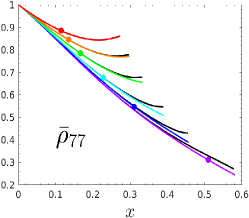
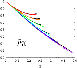
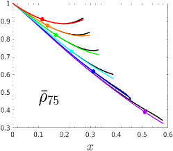
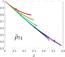
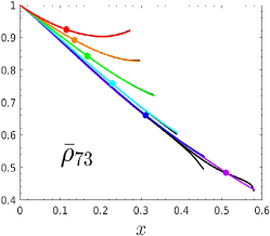
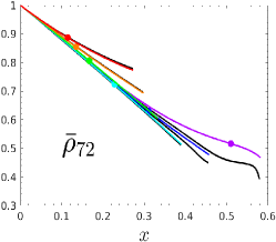
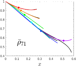
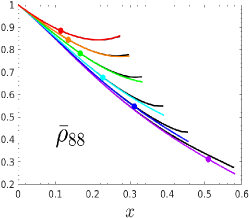
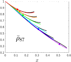
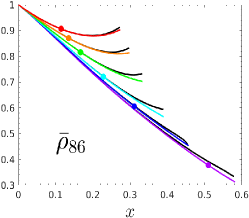
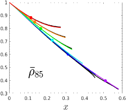
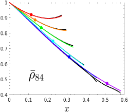
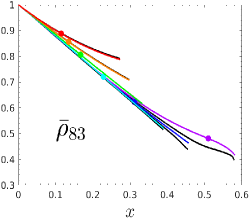
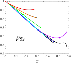
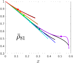
Figure 2: Comparison between the factorized and resummed analytical $\bar{\rho}_{{\ell m}}$ (colored lines) and the corresponding numerical (exact) functions (black lines) for ${\ell}=7,8$ and for values of the spin parameter ${\hat{a}}=(-0.99,-0.5,0,0.5,0.8,0.99)$ (red, orange, green, cyan, blue and purple, respectively). On the $x$-axis we have $x=\Omega^{2/3}$ and the filled circles mark the LSO location. These plots are obtained using 6 PN information for all the modes except for $\bar{\rho}_{73}$ and $\bar{\rho}_{72}$, that employ 8PN information, and for $\bar{\rho}_{71}$ that uses 5PN orders. The Padé approximants used for $\bar{\rho}_{\ell m}^{\rm orb}$ are listed in the second column of Table 3.

Table 3: Padé approximants used for the orbital part of the higher multipoles $\ell=7,8$ and corresponding relative differences $(\rho^{\rm num}_{\ell m}-\bar{\rho}^{\rm analyt}_{\ell m})/\rho^{\rm num}_{\ell m}$ at LSO for different spin values. The largest differences occur for ${\hat{a}}=+0.99$.

$(\ell,m)$	Padé	$-0.99$	$-0.5$	0	+0.5	+0.99
$(7,7)$	$P^{6}_{0}$	$-6\cdot 10^{-6}$	$2\cdot 10^{-5}$	$1\cdot 10^{-4}$	$9\cdot 10^{-4}$	$6\cdot 10^{-2}$
$(7,6)$	$P^{4}_{2}$	$2\cdot 10^{-3}$	$1\cdot 10^{-3}$	$2\cdot 10^{-4}$	$-1\cdot 10^{-3}$	$4\cdot 10^{-2}$
$(7,5)$	$P^{4}_{2}$	$2\cdot 10^{-5}$	$7\cdot 10^{-5}$	$2\cdot 10^{-4}$	$9\cdot 10^{-4}$	$3\cdot 10^{-2}$
$(7,4)$	$P^{4}_{2}$	$2\cdot 10^{-3}$	$1\cdot 10^{-3}$	$4\cdot 10^{-5}$	$-3\cdot 10^{-3}$	$-3\cdot 10^{-2}$
$(7,3)$	$P^{6}_{2}$	$5\cdot 10^{-7}$	$1\cdot 10^{-6}$	$2\cdot 10^{-6}$	$-6\cdot 10^{-5}$	$-4\cdot 10^{-3}$
$(7,2)$	$P^{8}_{0}$	$2\cdot 10^{-3}$	$1\cdot 10^{-3}$	$-4\cdot 10^{-7}$	$-3\cdot 10^{-3}$	$-1\cdot 10^{-1}$
$(7,1)$	$P^{2}_{3}$	$2\cdot 10^{-6}$	$4\cdot 10^{-5}$	$1\cdot 10^{-6}$	$-3\cdot 10^{-4}$	$-5\cdot 10^{-2}$
$(8,8)$	$P^{6}_{0}$	$-7\cdot 10^{-6}$	$2\cdot 10^{-5}$	$1\cdot 10^{-4}$	$9\cdot 10^{-4}$	$5\cdot 10^{-2}$
$(8,7)$	$P^{4}_{2}$	$2\cdot 10^{-3}$	$1\cdot 10^{-3}$	$3\cdot 10^{-4}$	$-9\cdot 10^{-4}$	$5\cdot 10^{-2}$
$(8,6)$	$P^{4}_{2}$	$2\cdot 10^{-5}$	$7\cdot 10^{-5}$	$3\cdot 10^{-4}$	$1\cdot 10^{-3}$	$4\cdot 10^{-2}$
$(8,5)$	$P^{4}_{2}$	$2\cdot 10^{-3}$	$1\cdot 10^{-3}$	$7\cdot 10^{-5}$	$-2\cdot 10^{-3}$	$-2\cdot 10^{-2}$
$(8,4)$	$P^{4}_{2}$	$9\cdot 10^{-6}$	$3\cdot 10^{-5}$	$9\cdot 10^{-5}$	$2\cdot 10^{-4}$	$-4\cdot 10^{-2}$
$(8,3)$	$P^{1}_{5}$	$2\cdot 10^{-3}$	$1\cdot 10^{-3}$	$2\cdot 10^{-6}$	$-2\cdot 10^{-3}$	$-8\cdot 10^{-2}$
$(8,2)$	$P^{5}_{1}$	$2\cdot 10^{-6}$	$1\cdot 10^{-5}$	$7\cdot 10^{-6}$	$-1\cdot 10^{-4}$	$-1\cdot 10^{-1}$
$(8,1)$	$P^{3}_{3}$	$2\cdot 10^{-3}$	$1\cdot 10^{-3}$	$-1\cdot 10^{-6}$	$-2\cdot 10^{-3}$	$-7\cdot 10^{-2}$

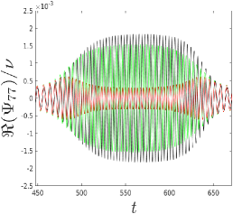
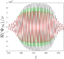
Figure 3: High spin and zoom-whirl behavior: left panel, trajectory for $e=0.3$, ${\hat{a}}=0.9$ and $p=p_{s}+0.01\simeq 2.615$. Middle and right panels: waveform comparison for $(\ell,m)=(7,7)$ and $(7,6)$ multipoles. Black lines: numerical data. Red lines: analytical waveform with the circular $\rho_{\ell m}$ in PN-expanded form at 6 PN. Green lines: analytical waveform with the factorized and resummed $\bar{\rho}_{\ell m}$, always at 6 PN. The resummation is essential to obtain a reasonably good agreement between the analytical and numerical waveforms.

The residual amplitude corrections $\rho_{{\ell m}}$ introduced in Eq. (14) are a crucial building block of any EOB waveform model and need a careful analytical treatment. In fact, although they are originally defined as PN series Damour et al. (2009), they may need additional resummation procedures to improve their strong-field behavior. The various PN truncations of the $\rho_{\ell m}$’s, either in the spinning or nonspinning case, typically oscillate around the function computed numerically solving the Teukolsky equation. A straight Padé approximant is not the most suitable choice, as pointed out in Nagar and Shah (2016); Messina et al. (2018). By contrast, Refs. Nagar and Shah (2016); Messina et al. (2018) suggested a different resummation scheme that: (i) first factorizes out the orbital, spin-independent, part and (ii) resums the orbital and spinning factors using, respectively, a Padé approximant and an inverse Taylor resummation scheme. The choice of the Padé approximant is partly arbitrary and is guided by the comparisons with the numerical results. In Refs. Nagar and Shah (2016); Messina et al. (2018) the resummation scheme was applied to all multipoles up to $\ell=6$. For our flux comparisons, especially in the presence of zoom-whirl orbits, we found it useful to apply the same scheme to the $\ell=7$ and $\ell=8$ modes. Let us recall the main elements of the procedure. As a first step, the orbital part is factorized as follows

$$\rho_{{\ell m}}(x)=\rho_{{\ell m}}^{\rm orb}(x)+\rho_{{\ell m}}^{\rm S}(x)=\rho_{{\ell m}}^{\rm orb}(x)\hat{\rho}_{{\ell m}}^{\rm S}(x),$$ (33)

where $\hat{\rho}_{{\ell m}}^{\rm S}=T_{n}\left[1+\rho_{{\ell m}}^{\rm S}/\rho_{{\ell m}}^{orb}\right]$ and $T_{n}$ indicates the Taylor expansion at the $n$th-PN order. Then a Padé approximant $P^{i}_{j}$ is used for the orbital part and an inverse Taylor scheme for the spin-part:

$$\begin{split}\bar{\rho}_{{\ell m}}^{\rm orb}(x)&=P^{i}_{j}\left(\rho_{{\ell m}}^{\rm orb}(x)\right),\\ \bar{\hat{\rho}}_{{\ell m}}^{\rm S}(x)&=\left(T_{n}\left[\left(\hat{\rho}_{{\ell m}}^{\rm S}(x)\right)^{-1}\right]\right)^{-1}.\end{split}$$ (34)

The final result is given by the product of the two resummed factors

$$\bar{\rho}_{{\ell m}}(x)=\bar{\rho}_{{\ell m}}^{\rm orb}(x)\bar{\rho}_{{\ell m}}^{\rm S}(x).$$ (35)

We extend this approach to $\ell=7$ and $\ell=8$ modes using the PN series of the relativistic amplitude corrections for a test-particle on circular orbits around a Kerr black hole Fujita (2015). We use 6 PN accuracy for almost all the multipoles, the only exceptions are the (7,3) and (7,2) modes where we have used 8 PN information, and the (7,1) mode where we have resummed the series truncated at 5 PN. This choice is motivated by the significantly better agreement with numerical data achieved for high spin. However, these modes are highly subdominant and their contribution to the fluxes is mostly negligible. In fact, the contribution to the angular momentum flux of the modes with ${\ell}=7,8$ and $m\leq 3$ all summed together in the case $({\hat{a}},e,p)=(0.9,0,p_{s}+0.01)$ is $2\cdot 10^{-7}\%$, while in all the other simulations it is even smaller. In practice, all the relevant information in the resummed $\bar{\rho}_{\ell m}$ is at 6 PN. We also mention in passing that for extremal cases with ${\hat{a}}>0.99$, the $\bar{\rho}_{81}$ has a pole in the spin factor, so that one is obliged to use the plain PN series. Nonetheless, in this work we consider spins only up to ${\hat{a}}=0.9$, then we will always use the resummed $\bar{\rho}_{\ell m}$. This problem is not present for any of the other modes. The reliability of the resummation has been tested using circular frequency-domain data obtained by S. Hughes kindly made available to us Taracchini et al. (2013). The comparisons between resummed analytical expressions and numerical data are shown in Fig. 2, while the list of Padé used is reported in Table 3 with the corresponding relative differences at the Last Stable Orbit (LSO). We address the reader to Ref. Messina et al. (2018) for complementary technical details. The resummation is especially relevant for prograde zoom-whirl orbits around fast spinning black holes, as shown in Fig. 3 for the illustrative case $(e,{\hat{a}})=(0.3,0.9)$. In fact, during the circular whirl the amplitude of the nonresummed $\rho_{77}$ at 6 PN becomes unphysically small (red line). This behavior is mostly solved by the resummation procedure exposed above, leading to a better agreement with numerical data (green lines in Fig. 3). Note however that the analytical waveform underestimates the exact result, as typical of prograde orbits around fast spinning black holes. We will discuss this issue in more details in Sec. IV. Finally, note that in Fig. 3 we are not using any PN correction for the residual phase of the tail factor, and this leads to a great phase-difference between numerical and analytical waveforms during the circular whirl. We will address this issue in the next subsection.

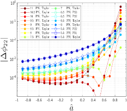
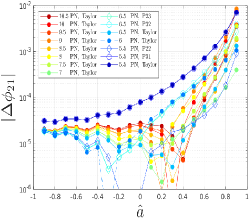
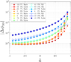
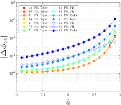
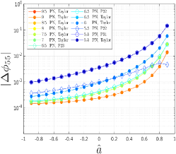
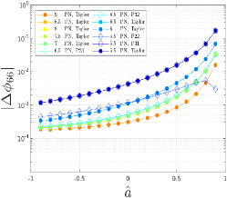
Figure 4: Phase difference between numerical and analytical waveform multipoles for different truncation of the $\delta_{\ell m}$ series (filled markers) and Padé resummations obtained with Eq. (37) (empty markers) for the near circular simulations ($r=r_{\rm LSO}+0.01$). Note the different vertical scale for the (2,1) mode.

III.4 Impact of residual waveform phases $\delta_{\ell m}$

To improve the circular part of the waveform, we have incorporated high-order PN information also in the residual phases $\delta_{\ell m}$ of Eq. (14). In particular, we have exploited various PN truncations of the 11 PN series for a test-particle on circular orbits around a Kerr black hole Fujita (2015). We have also tested the resummation scheme introduced in Damour et al. (2013), where the resummed phases are obtained by factorizing the leading order $\delta_{\ell m}^{\rm LO}$ contribution and then using a Padé approximant $P^{i}_{j}$ for the remaining correcting factor $\hat{\delta}_{\ell m}$, explicitly:

$$\delta_{\ell m} =\delta_{\ell m}^{\rm LO}+\delta_{\ell m}^{\rm NLO}+\dots=\delta_{\ell m}^{\rm LO}\hat{\delta}_{\ell m},$$ (36)

$$\bar{\delta}_{\ell m} =\delta_{\ell m}^{\rm LO}P^{i}_{j}[\hat{\delta}_{\ell m}].$$ (37)

We report in Fig. 4 the phase differences between numerical and analytical circular waveforms, either with the PN-expanded $\delta_{\ell m}$ (at various PN truncations) or with the resummed $\bar{\delta}_{\ell m}$. We consider some of the most relevant modes and only consider radii close to the LSO ($r=r_{\rm LSO}+0.01$). For moderate spins ($\hat{a}\lesssim 0.5$), we see that the analytical/numerical phase agreement of the dominant mode is improved by increasing the PN order of $\delta_{22}$. Nonetheless, when the spin increases, the series beyond 8 PN become unreliable. For the subdominant modes, the PN series at high order are reliable also for ${\hat{a}}\gtrsim 0.5$, even if for $\delta_{21}$ and $\delta_{33}$ some series at lower order give similar (or better) agreements.

Applying the resummation scheme of Eq. (37) at 5.5 PN, we see that the most suitable choice is the Padé $P^{2}_{2}$. The resummation provides a better numerical/analytical agreement than the corresponding Taylor-expanded series at 5.5 PN. Nonetheless, the Taylor expanded $\delta_{22}$ at 6 or 7.5 PN yields comparable, or even better, agreement with numerical waveforms. For prograde orbits with ${\hat{a}}\gtrsim 0.3$, the resummation of the ${\ell}=m$ subdominant modes provides a more faithful description than the Taylor expanded series at 6.5 PN, as shown in Fig. 4. For even higher spins (${\hat{a}}\gtrsim 0.8$), the resummed $\bar{\delta}_{\ell m}$ outperform also the series beyond 7 PN. The hierarchy of the analytical/numerical phase difference is different for the (2,1) mode, but in that case all the phase differences are below $0.01$ radians. A similar argument holds at larger radii, even if for distant simulation is less straightforward to evaluate the goodness of the analytical choice, since the comparisons are affected by the numerical errors.

Note in passing that, while spurious poles are absent in $\ell=m$ and $(2,1)$ modes of the resummed $\delta_{\ell m}$ with Padé $P^{2}_{2}$, they may occasionally appear in some other subdominant modes. Finally, we have also successfully applied the resummation scheme at 6.5 PN accuracy as shown in Fig. 4. By contrast, when working at 7.5 PN, one finds spurious poles even in the $(2,2)$ mulitpole, either with Padé $P^{4}_{2}$ or $P^{3}_{3}$, so that the resummation is not robustly applicable in this case.

Generally speaking, the resummed $\bar{\delta}_{\ell m}$ yield a better phasing agreement with the numerical results. In particular they are more robust than the high-order PN truncations for prograde orbits around fast-spinning black hole. Nonetheless, in order to choose a compromise between accuracy and analytical simplicity, we have decided to consider the series truncated at 7.5 PN as our preferred choice.

For noncircular simulations, the $\delta_{\ell m}$ are relevant during the circular whirl of zoom-whirl orbits, but are less significant for the other eccentric orbits. For higher spins, the analytical choice is more relevant since the separations reached are closer to the light ring and thus the PN series are applied in stronger fields.

IV Fluxes phenomenology and analytical/numerical comparisons

Now that we have clarified the various analytical structures involved, let us turn to discussing the comparisons between analytical and numerical fluxes. The final goal of this procedure is to identify the range of validation of the analytical expressions so that they can consistently used to drive an eccentric inspiral. We do these comparisons in two complementary ways. In Sec. IV.1 we discuss instantaneous fluxes, while in Sec. IV.2 we discuss orbital averaged fluxes so to easily gain a global picture for all values of $(e,\hat{a})$.

IV.1 Instantaneous fluxes

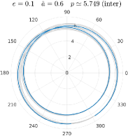
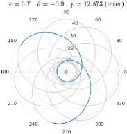
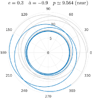
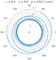
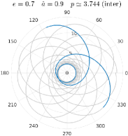
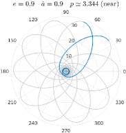
Figure 5: Geodesic equatorial orbits for different ($e$, ${\hat{a}}$, $p$) configurations, including the so-called zoom-whirl behavior (bottom-right panel). We have highlighted one radial orbit for each configuration. The corresponding fluxes and waveforms are shown in Fig. 6 and Fig. 10.

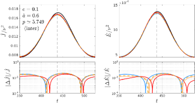
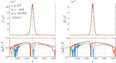
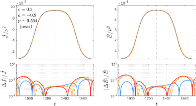
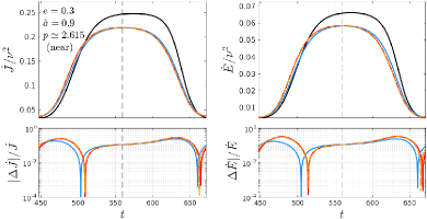
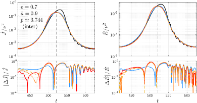
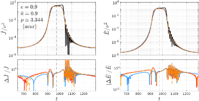
Figure 6: Angular momentum, $\dot{J}$, and energy, $\dot{E}$, fluxes at infinity corresponding to the equatorial orbital dynamics shown in Fig. 5. The top panel of each plot focuses on a time interval around a periastron passage, that is indicated by a vertical dashed line. The numerical fluxes (black) are contrasted with four different analytical fluxes (in color). ${\dot{F}_{\rm NP}}$ (red), ${\dot{F}_{\rm ANP}}$ (dashed orange), ${\dot{F}_{\rm old}}$ (dotted orange), ${\dot{F}_{h_{{\ell m}}}}$ (light blue). The bottom panel of each plot shows the absolute value of the corresponding relative difference.

The phenomenology of the instantaneous GW fluxes of a particle on an eccentric orbit around a Kerr black hole depends on the eccentricity, $e$, semilatus rectum, $p$, and black hole spin, $\hat{a}$. To set the stage of our discussion, let us take a sample of illustrative configurations that survey the different phenomenologies. The selected parameters and trajectories are shown in Fig. 5. We considered both mildly eccentric and highly eccentric configurations, some of these showing the so-called zoom-whirl behavior Glampedakis and Kennefick (2002), involving several revolutions around the central body near periastron (see e.g. bottom right panel of the Fig. 5). In particular, an interesting feature arises from the fact that, when a corotating test-particle gets close to the light ring at high velocity, the QNMs of the central black hole can be excited, producing high-frequency oscillations (usually addressed as wiggles) in the radiated GWs at infinity Kojima and Nakamura (1984). This phenomenon has been recently analyzed in details both using TD and FD codes Rifat et al. (2019); Thornburg et al. (2020). Moreover, the QNM excitation leads to strongly asymmetric fluxes with respect to the periastron passage. The excitations become more relevant when the velocity of the test-particle increases and when the periastron of the orbits gets closer to the light ring. Moreover, the damping time of the QNMs increases significantly for high spins, therefore these excitations are mostly of interest for extremal black holes (${\hat{a}}\gtrsim 0.99$). Nonetheless, QNMs excitations are present also in less extreme cases, as pointed out in Thornburg et al. (2020). These effects are particularly relevant for prograde zoom-whirl orbits with high eccentricity around fast spinning black hole since the periastron can get very close to the light ring. The energy and angular momentum fluxes corresponding to the trajectories of Fig. 5 are shown in Fig. 6. The main aim of the figure is to compare the numerical fluxes (in black) with the different flavors of the analytical fluxes (in color), but we will comment this in detail below. Still, one can clearly see how the QNMs excitations build up when $p$ is changed so to allow the system to pass close to the light ring. This occurs either in the case of extreme eccentricity or in case of zoom-whirl behavior.

The EOB analytical waveform model is not designed to incorporate QNMs-related effects. Despite this, one can achieve a reasonable qualitative and quantitative agreement also when they are present. For each configuration, Fig. 6 contrast the exact, numerical, fluxes with four different analytical approximations:

• ${\hat{{\cal F}}_{\varphi}^{\rm NP}}$ from Eq. (25) that corresponds to the ${\dot{F}_{\rm NP}}$ fluxes. In this case the angular radiation reaction has the noncircular (2,2) Newtonian prefactor ${{\hat{f}_{\varphi,22}^{\rm N_{nc}}}}$ in the (2,2) multipole. This is now the standard prescription in state-of-the-art EOB waveform model Nagar et al. (2021b).

• ${\hat{{\cal F}}_{\varphi}^{\rm old}}$ from Eq. (22) from which we compute the ${\dot{F}_{\rm old}}$ fluxes. In ${\hat{{\cal F}}_{\varphi}^{\rm old}}$, the noncircular (2,2) Newtonian prefactor ${{\hat{f}_{\varphi,22}^{\rm N_{nc}}}}$ is a global factor.

• ${\hat{{\cal F}}_{\varphi}^{\rm ANP}}$ from Eq. (26), that provides the ${\dot{F}_{\rm ANP}}$ fluxes. In this case we consider all the noncircular Newtonian prefactors up to ${\ell}=6$.

• ${\dot{F}_{h_{{\ell m}}}}$, the fluxes obtained directly plugging the analytical waveform $h_{\ell m}$ in Eq. (13) and summing over all multipoles up to $\ell_{\rm max}=8$. These quantities are exhibited as blue lines in the plots.

The various analytical choices offer substantially comparable approximations to the numerical fluxes. In order to establish a preferred one, we need an efficient way to perform analytical/numerical comparisons all over the $(e,p,\hat{a})$ parameter space. We do so in the next section studying the behavior of orbital averaged fluxes.

IV.2 Averaged fluxes

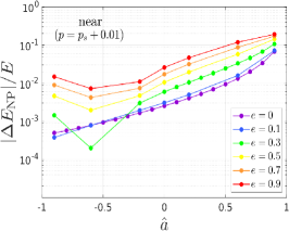
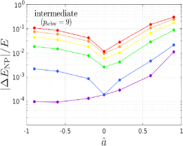
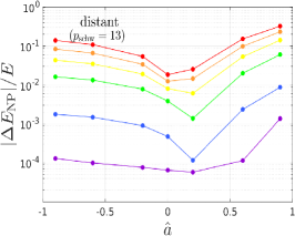
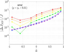
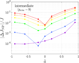
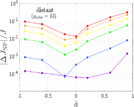
Figure 7: Relative differences between numerical and analytical averaged fluxes plotted against the spin (absolute value, logarithmic scale). We consider ${\dot{F}_{\rm NP}}$, the fluxes with the (2,2) general Newtonian prefactor of Eq. (III.2) in the (2,2) multipole.

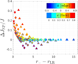
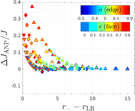
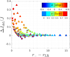
Figure 8: Left panel: relative differences $\Delta J_{\rm NP}/J\equiv({\langle{\dot{J}_{\rm teuk}}\rangle}-{\langle{\dot{J}_{\rm NP}}\rangle})/{\langle{\dot{J}_{\rm teuk}}\rangle}$ for the fluxes with the (2,2) general Newtonian prefactor in the (2,2) multipole plotted against the distance between the light ring and the periastron. The face color of the markers indicates the eccentricity, while the edge color indicates the spin. The shape of the markers is related to the rule used for the semilatus rectum: the reverse triangle indicates the near simulations, the diamond is for the intermediate simulations and the triangle pointing upward indicates the distant simulations. Other two panels: same scheme, but for $J_{\rm ANP}$ and $J_{\rm old}$. See Fig. 21 for analogous plots with ${\dot{J}_{h_{{\ell m}}}}$ and also with the energy fluxes.

In order to systematically and efficiently test the various analytical expressions discussed above, we consider the $\nu$-normalized fluxes averaged over a radial period $T_{r}$

$${\langle\dot{F}\rangle}=\frac{1}{T_{r}}\int_{0}^{T_{r}}\frac{\dot{F}}{\nu^{2}}\,dt,$$ (38)

and we calculate the relative differences between numerical and analytical fluxes. We have considered all the analytical prescriptions discussed in Sec. III.2: ${\dot{F}_{\rm NP}}$, ${\dot{F}_{\rm old}}$, ${\dot{F}_{\rm ANP}}$ and ${\dot{F}_{h_{{\ell m}}}}$. All the values for the relative differences between numerical and analytical averaged fluxes can be found in Appendix D.

Before analyzing the different analytical prescriptions, we discuss some general features of the fluxes over the parameter space. As a priori expected, the analytical/numerical disagreement grows both with spin and eccentricity, since the periastron of prograde orbits can get very close to the light ring for high spin parameters and high eccentricity. In strong fields, the PN series employed in our model lose their reliability, even if strengthened by a proper resummation. In particular, from the relative differences between numerical and ${\dot{F}_{\rm NP}}$ fluxes reported in Fig. 7, it is possible to see that the spin is a relevant source of disagreement regardless of eccentricity. On the other hand, the eccentricity is also crucial for the reliability of the fluxes, both for the lack of noncircular information in the angular radiation reaction beyond the Newtonian order and for the approaching of the periastron to stronger fields for higher eccentricities. The last issue can be easily seen in Fig. 8, where in the first panel we have plotted the same numerical/analytical relative differences of the angular momentum fluxes versus the distance between the light ring and the periastron. In the other two panels of Fig. 8 we have shown the differences for the other radiation reactions of Eq. (26) and Eq. (22). The analogous plots for the other analytical fluxes can be found in Appendix D, but the general features discussed so far are valid for any of them.

In order to decide which radiation reaction adopt to drive the transition from inspiral to plunge (that we shall often address as insplunge in the following), we focus on the three analytical angular momentum fluxes that are strictly linked to an analytical prescription of the radiation reaction: ${\dot{J}_{\rm NP}}$, ${\dot{J}_{\rm old}}$, and ${\dot{J}_{\rm ANP}}$ (see Sec. III.2 for more details). Note that the analytical prescription of $\hat{{\cal F}}_{r}$ is the same in all the radiation reactions tested in this work, then to analyze them it is sufficient to study the angular momentum fluxes. The fluxes computed from the EOB waveform (i.e. ${\dot{J}_{h_{{\ell m}}}}$) are less informative since they are not related to the radiation reaction and we will not discuss them in details.

As a first step, we focus on the two averaged analytical fluxes with only the (2,2) noncircular Newtonian prefactor ${{\hat{f}_{\varphi,22}^{\rm N_{nc}}}}$, i.e. ${\langle{\dot{J}_{\rm old}}\rangle}$ and ${\langle{\dot{J}_{\rm NP}}\rangle}$. These fluxes are computed, respectively, using the angular radiation reactions ${\hat{{\cal F}}_{\varphi}^{\rm old}}$ from Eq. (22) and ${\hat{{\cal F}}_{\varphi}^{\rm NP}}$ from Eq. (25). We start by noting that ${\hat{{\cal F}}_{\varphi}^{\rm NP}}$ is theoretically more consistent than ${\hat{{\cal F}}_{\varphi}^{\rm old}}$ since the former includes the (2,2) noncircular Newtonian prefactor only in the (2,2) multipole, while in the older prescription the noncircular correction is treated as a global factor, and therefore affects even the subdominant modes. Nonetheless, for retrograde orbits ${\langle{\dot{J}_{\rm old}}\rangle}$ has a better numerical/analytical agreement than ${\langle{\dot{J}_{\rm NP}}\rangle}$. In fact, the latter overestimates significantly the numerical fluxes, especially at high eccentricity, as can be seen from Fig. 8. This can be explained by noting that the dominant contribution to the averaged fluxes occurs at periastron, where we have ${{\hat{f}_{\varphi,22}^{\rm N_{nc}}}}<1$. Then, the lack of noncircular corrections in the subdominant multipoles of ${\langle{\dot{J}_{\rm NP}}\rangle}$ leads to an overestimate of the numerical result. On the other hand, in ${\langle{\dot{J}_{\rm old}}\rangle}$ the noncircular correction ${{\hat{f}_{\varphi,22}^{\rm N_{nc}}}}$ is a global factor and thus artificially reduces the contribution of the subdominant modes, fixing the overestimate. Nonetheless, this is an artifact and the old radiation reaction is not solid: adding noncircular information beyond the Newtonian level in the angular radiation reaction would probably improves ${\langle{\dot{J}_{\rm NP}}\rangle}$, but not ${\langle{\dot{J}_{\rm old}}\rangle}$.
In the Schwarzschild case or for prograde orbits, the new prescription is more accurate. In fact, for spins aligned with the orbital angular momentum, the two analytical prescriptions generally underestimate the numerical fluxes, and therefore a global factor that is smaller than $1$ at periastron worsen the numerical/analytical agreement, making the older prescription less accurate.

Let now consider the averaged fluxes ${\langle{\dot{J}_{\rm ANP}}\rangle}$, that are computed using ${\hat{{\cal F}}_{\varphi}^{\rm ANP}}$ from Eq. (26) and thus include all the noncircular corrections up to ${\ell}=6$. Comparing them with the ${\langle{\dot{J}_{\rm NP}}\rangle}$ fluxes, we can see that the ANP prescription is more reliable for retrograde orbits, but produces bigger relative differences with numerical data in the nonspinning case and for prograde orbits. The reason of this behavior is again related to the fact that at periastron we have ${\hat{f}_{\varphi,{\ell m}}^{\rm N_{nc}}}<1$, as discussed above.

Table 4: Averaged analytical fluxes for test-particle on eccentric orbits around a Schwarzschild black hole compared with numerical results, $\Delta J_{\rm NP}/J=({\langle{\dot{J}_{\rm teuk}}\rangle}-{\langle{\dot{J}_{\rm NP}}\rangle})/{\langle{\dot{J}_{\rm teuk}}\rangle}$. For $p\leq 13$, the numerical fluxes in this table are obtained with Teukode and are a subset of the ones shown in Appendix D. The fluxes with greater semilatera recta are computed with RWZhyp.

$e$	$p$	${\langle\dot{J}_{\rm num}\rangle}$	${\langle{\dot{J}_{\rm NP}}\rangle}$	$\Delta J_{\rm NP}/J$
$0.1$	$6.21$	$10.5396$	$10.5076$	$3.0\cdot 10^{-3}$
$0.1$	$9$	$0.85442$	$0.85401$	$4.9\cdot 10^{-4}$
$0.1$	$13$	$0.30867$	$0.30857$	$3.2\cdot 10^{-4}$
$0.1$	$21$	$0.10208$	$0.10207$	$7.9\cdot 10^{-5}$
$0.1$	$31$	$0.04445$	$0.04446$	$-7.0\cdot 10^{-5}$
$0.3$	$6.61$	$8.73092$	$8.67715$	$6.2\cdot 10^{-3}$
$0.3$	$9$	$0.97246$	$0.96998$	$2.6\cdot 10^{-3}$
$0.3$	$13$	$0.33935$	$0.33855$	$2.3\cdot 10^{-3}$
$0.3$	$21$	$0.11055$	$0.11048$	$5.9\cdot 10^{-4}$
$0.3$	$31$	$0.04786$	$0.04789$	$-6.6\cdot 10^{-4}$
$0.5$	$7.01$	$9.22978$	$9.12458$	$1.1\cdot 10^{-2}$
$0.5$	$9$	$1.23262$	$1.22659$	$4.9\cdot 10^{-3}$
$0.5$	$13$	$0.40329$	$0.40085$	$6.0\cdot 10^{-3}$
$0.5$	$21$	$0.12784$	$0.12760$	$1.9\cdot 10^{-3}$
$0.5$	$31$	$0.05479$	$0.05488$	$-1.8\cdot 10^{-3}$
$0.7$	$7.41$	$10.5483$	$10.3521$	$1.9\cdot 10^{-2}$
$0.7$	$9$	$1.69513$	$1.68505$	$5.9\cdot 10^{-3}$
$0.7$	$13$	$0.50634$	$0.50113$	$1.0\cdot 10^{-2}$
$0.7$	$21$	$0.15477$	$0.15408$	$4.4\cdot 10^{-3}$
$0.7$	$31$	$0.06542$	$0.06562$	$-3.1\cdot 10^{-3}$
$0.9$	$7.81$	$12.5209$	$12.1752$	$2.8\cdot 10^{-2}$
$0.9$	$9$	$2.49117$	$2.47585$	$6.1\cdot 10^{-3}$
$0.9$	$13$	$0.65853$	$0.64984$	$1.3\cdot 10^{-2}$
$0.9$	$21$	$0.19258$	$0.19098$	$8.3\cdot 10^{-3}$
$0.9$	$31$	$0.08011$	$0.08041$	$-3.8\cdot 10^{-3}$

As anticipated, the fluxes ${\langle{\dot{J}_{\rm NP}}\rangle}$ are the most accurate in the Schwzarschild case. As can be seen from Table 4, in the nonspinning case this prescription is highly reliable for every configuration, yielding relative differences always below the $3\%$, even for orbits with high eccentricity. Instead, for the other analytical prescriptions, the relative difference can be even $>7\%$, as shown in Table 8 and Table 9. Note that for $p\geq 9$, the accuracy of our analytical model is consistent with the averaged eccentric fluxes at 10 PN computed in Refs. Munna et al. (2020); Munna (2020), but the EOB model remains solid even for smaller semilatera recta thanks to a robust resummation of the PN series.

In conclusion, considering that (i) the old prescription is not theoretically accurate, (ii) the radiation reaction with all the multipoles does not drastically improves the model for moderate eccentricities and moderate spins despite being much more complicated, (iii) the fluxes ${\langle{\dot{J}_{\rm NP}}\rangle}$ are the most faithful in the nonspinning case, we decide to use in our eccentric insplunge simulations the angular radiation reaction ${\hat{{\cal F}}_{\varphi}^{\rm NP}}$ from Eq. (25).

With this choice, the energy and angular momentum fluxes have an agreement of few percents for moderate eccentricities ($e\lesssim 0.3$), even if for prograde orbits the spin reduces the maximum eccentricity up to which the model has good agreement with the numerical results. In the worst case, i.e. the one with ${\hat{a}}=0.9$, $e=0.9$ and ’distant’ semilatus rectum ($p\simeq 5.557$), we get relative differences of the $33\%$ and $31\%$ for the energy and angular momentum fluxes, respectively (see Table 7). Note that the worst case is not a near simulation, since in that case the lack of noncircular information is compensated by the zoom-whirl behavior.

IV.3 Subdominant multipoles

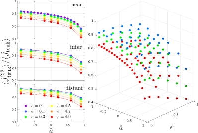
Figure 9: Relative contributions of the ${\ell}=|m|=2$ modes to the total averaged angular momentum flux over the parameter space. In the 3D plot we show all the near (red), intermediate (green) and distant (blue) simulations, while on the left we have separated the three different classes.

Let us finally discuss in some detail the separate contribution of the various subdominant modes to the angular momentum flux. Subdominant modes become more and more relevant for high spins, high eccentricities and for semilatera recta near the separatrix as shown in Fig. 9, where we have plotted the ${\ell}=|m|=2$ relative contribution to the total averaged angular momentum flux. In the distant circular case with ${\hat{a}}=-0.9$, it provides the $92.9\%$ of the total flux; by contrast, for the zoom-whirl orbit with ${\hat{a}}=0.9$ and $e=0.9$, its contribution is only of the $42.6\%$. In the former case, the relative contribution of the ${\ell}=8$ modes summed together is $3.9\cdot 10^{-5}\%$, while in the latter is $2.2\%$. For the complete list of the relative ${\ell}$-contributions to the angular momentum flux, see Appendix E.

The analytical subdominant modes tend to have greater discrepancies with the corresponding numerical multipoles than the dominant one. In the noncircular case, this result is trivial for the fluxes with only the (2,2) noncircular Newtonian prefactor, but holds even if we include the noncircular corrections for each multipole.

V Multipolar waveform

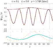
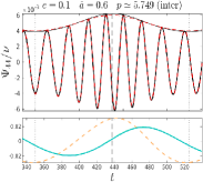
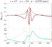
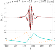
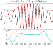
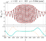
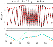
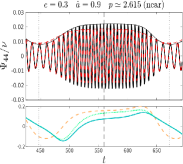
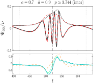
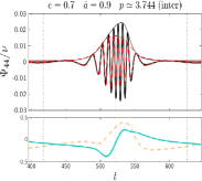
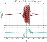
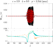
Figure 10: Numerical (black) and EOB (red dashed) ${\ell}=m=2$ and ${\ell}=m=4$ multipoles corresponding to the dynamics shown in Fig. 5. For each multipole, we report the relative amplitude difference (dashed orange) and the phase difference (light blue). We report also the phase differences for the waveform with the residual tail factor at 6 PN (dotted green). The vertical lines mark the periastron and the apastron.

V.1 Geodesic, equatorial motion

Let us turn now to discussing the performance of the analytical multipolar waveform. Reference Chiaramello and Nagar (2020) already pointed out the fairly good analytical/numerical agreement that can be obtained only with the prescription of replacing the quasi-circular Newtonian prefactor by the general one. A systematic multipole by multipole analysis shows that the relative discrepancies increase in the subdominant multipoles, i.e. the $(2,2)$ is in general the most reliable, similarly to what discussed for the subdominant contribution to the fluxes. In particular, in the absence of QNMs excitations, the relative differences between analytical and numerical amplitudes is generally smaller than the analogous ones for the fluxes. Figure 10 highlights the analytical/numerical agreement for the $\ell=m=2$ and $\ell=m=4$ modes obtained from the six illustrative configurations of Fig. 5. For two configurations, we explicitly show in Appendix C the comparison for almost all other multipoles, see Fig. 16 and 17. For each configuration we compare, in the top panel, the real part of the analytical and numerical waveform burst emitted around the periastron. For the zoom-whirl configuration this corresponds to the many GW cycles corresponding to the quasi-circular regime. In the bottom panel we show the analytical/numerical phase difference $\Delta\phi=\phi^{\rm analytical}_{\ell m}-\phi^{\rm numerical}_{\ell m}$ and relative amplitude difference $|A^{\rm analytical}_{\ell m}-A^{\rm numerical}_{\ell m}|/A^{\rm numerical}_{\ell m}$.

In Fig. 10 (as well as 16 and 17), the residual waveform phases $\delta_{\ell m}$ are kept at 7.5 PN accuracy, that is our default choice. Such high-PN accuracy is relevant for circular or zoom-whirl orbits, but it is less important for other eccentric configurations. In particular, for the intermediate configurations considered here they are practically equivalent, except for the high spin case ${\hat{a}}\simeq 0.9$, since the periastron occurs at small values of the radial separation. The periastron is, obviously, where the knowledge of high PN information matters most. To show this fact, we also report in Fig. 10 the phase differences obtained with $\delta_{\ell m}$ at 6 PN accuracy (green dotted online). Finally, note that the phase difference reaches its minimum near periastron. This suggests that in the eccentric case this quantity is dominated by the lack of high-order noncircular information in the waveform beyond the (leading-order) Newtonian level. This last sentence could also be justified noting that the discrepancies in the circular case are much smaller, as shown in Fig. 4.

V.2 Transition from eccentric inspiral, plunge, merger and ringdown

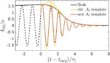
Figure 11: Ringdown modelization: transition from quasi-circular inspiral to plunge, merger and ringdown with $\nu=10^{-3}$ and ${\hat{a}}=0.8$. The time-scale is rescaled using $\tau_{1}=1/\alpha_{1}$. The new fitting template for the amplitude, Eq. (39) accurately reproduces the numerical data, while the standard one, proposed in Ref. Damour and Nagar (2014b), delivers an unphysical local maximum during ringdown.

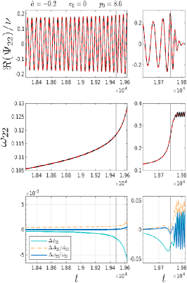
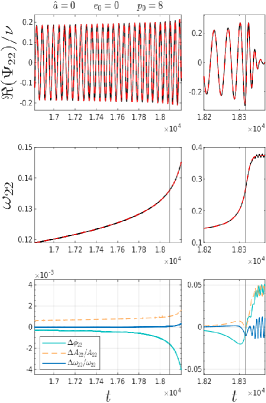
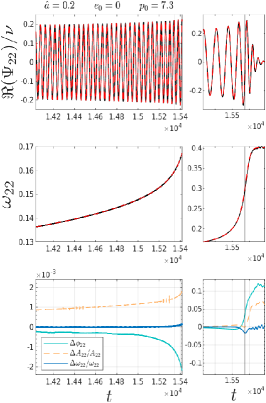
Figure 12: Comparison between numerical (black) and analytical (red) waveforms for the transition from circular inspiral to plunge, merger and ringdown. We report the comparisons for spins ${\hat{a}}=0,\pm 0.2$. The two vertical lines mark the LSO and the merger time. In the last panel of each comparison, we report the relative difference of the amplitude (orange) and frequency (blue) together with the phase difference (light blue) in radians.

Until now we have separately explored the quality of the analytical waveform and fluxes along eccentric geodesic orbit. The final aim of this work is to incorporate these two building blocks together in order to consistently drive an eccentric inspiral. The aim of this section is to discuss the complete resummed analytical waveform, that for simplicity we will call EOB waveform, obtained from an eccentric dynamics driven by the radiation reaction force discussed above. In doing so, we do not limit ourselves to the inspiral, but we proceed to plunge, merger and ringdown, building a suitable model for this latter. In this respect, the results we present here, that should be considered preliminary, complement and generalize previous work within the EOB approach in the extreme-mass-ratio limit Nagar et al. (2007); Damour and Nagar (2007); Yunes et al. (2011); Barausse et al. (2012a).

In particular, the analytical description of the ringdown stems from the effective model introduced in Ref. Damour and Nagar (2014b), that relies on a certain way of fitting NR waveform data. In current EOB models informed by NR simulations, and in particular TEOBResumS Nagar et al. (2019b, 2020), the model is fully informed by spin-aligned NR simulations up to mass ratio $q=18$, but relied on a limited amount of information coming from test-particle waveform data, i.e. only the values of amplitude and frequency at merger time. The reason is that the fitting template for the amplitude proposed in Ref. Damour and Nagar (2014b) and used in TEOBResumS Nagar et al. (2019b, 2020) is not reliable in the test-particle limit when the spin of central black hole is large. This fact is illustrated in Fig. 11. The black curves depict the amplitude (solid) and real part (dashed) of a quasi-circular, numerical waveform corresponding to $\hat{a}=0.8$ and $\nu=10^{-3}$. The yellow curves are the result of fitting the data with the amplitude template of Damour and Nagar (2014b). The unphysical peak in the postmerger is a recurrent feature, that, although practically negligible for small (or negative) values of ${\hat{a}}$ becomes predominant as the black hole spin grows.

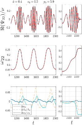
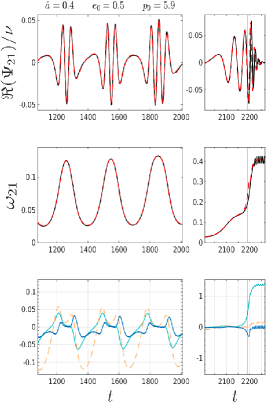
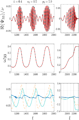
Figure 13: Comparison between numerical (black) and analytical (red dashed) complete waveform generated by a non-geodesic prograde orbit with initial eccentricity $e_{0}=0.5$ and semilatus rectum $p_{0}=5.9$ around a Kerr black hole with ${\hat{a}}=0.4$. The vertical line marks the merger time. In the last panel of each mode, we report the relative difference of the amplitude (orange) and frequency (blue) together with the phase difference (light blue) in radians.

This problem can be fixed increasing the flexibility of the amplitude template. Referring from now on to $\bar{h}$ as the QNM-rescaled ringdown waveform of Ref. Damour and Nagar (2014b) (see Eq. (1) therein) we adopt here the following function to model the amplitude

$$A_{\bar{h}}(\tau)=\left(\frac{c_{1}^{A}}{1+e^{-c_{2}^{A}\tau+c_{3}^{A}}}+c_{4}^{A}\right)^{\frac{1}{c_{5}^{A}}}\ ,$$ (39)

while for the phase we just follow the prescription of  Damour and Nagar (2014b) and use

$$\phi_{\bar{h}}(\tau)=-c_{1}^{\phi}\ln\left(\frac{1+c_{3}^{\phi}e^{-c_{2}^{\phi}\tau}+c_{4}^{\phi}e^{-2c_{2}^{\phi}\tau}}{1+c_{3}^{\phi}+c_{4}^{\phi}}\right),$$ (40)

where $\tau\equiv t-t_{\rm mrg}$. The merger time $t_{\rm mrg}$ is defined as the amplitude peak of the quadrupolar waveform. The only parameters to be fitted on numerical data are $c_{2}^{A}$, $c_{3}^{A}$, $c_{3}^{\phi}$ and $c_{4}^{\phi}$, while the others are determined requiring the correct late-time behavior. Note however that now the amplitude is fitted using two parameters, contrary to Ref. Damour and Nagar (2014b), that could employ a single fitting parameter. The constraints given by the late-time behavior of the ringdown are

$$c_{1}^{A} =\frac{c_{5}^{A}\alpha_{1}}{c_{2}^{A}}(A_{\rm mrg})^{c_{5}^{A}}e^{-c_{3}^{A}}\left(1+e^{c_{3}^{A}}\right)^{2},$$ (41)

$$c_{4}^{A} =(A_{\rm mrg})^{c_{5}^{A}}-\frac{c_{1}^{A}}{1+e^{c_{3}^{A}}},$$ (42)

$$c_{5}^{A} =-\frac{\ddot{A}_{\rm mrg}}{A_{\rm mrg}\alpha_{1}^{2}}+\frac{c_{2}^{A}}{\alpha_{1}}\frac{e^{c_{3}^{A}}-1}{1+e^{c_{3}^{A}}}\ ,$$ (43)

$$c_{2}^{\phi} =\alpha_{21},$$ (44)

$$c_{1}^{\phi} =\dfrac{1+c_{3}^{\phi}+c_{4}^{\phi}}{c_{2}^{\phi}(c_{3}^{\phi}+2c_{4}^{\phi})}\Delta\omega_{\rm mrg},$$ (45)

where $\alpha_{i}$ are the real parts of the QNM complex frequencies $\sigma_{i}\equiv\alpha_{i}+{\rm i}\omega_{i}$ (i.e., the inverse of the damping time), $\alpha_{21}\equiv\alpha_{2}-\alpha_{1}$, $A_{\rm mrg}$ is the amplitude at merger, $\ddot{A}_{\rm mrg}$ its second time-derivative, $\Delta\omega_{\rm mrg}\equiv\omega_{1}-M\omega_{\rm mrg}$ is the difference between the frequency at merger $\omega_{\rm mrg}$ and the imaginary part of the fundamental QNM frequency $\omega_{1}$. The red curves in Fig. 11 illustrate the accuracy of the new template amplitude. In principle, any EOB-based model for coalescing black hole binaries, like TEOBResumS Nagar et al. (2020), should correctly incorporate the test-mass limit. Due to this problem in the original waveform amplitude template, this is not the case of TEOBResumS, although large-mass-ratio waveforms look qualitatively and quantitatively essentially correct because of the inclusion of test-particle-informed fits for $(A_{\rm mrg},\omega_{\rm mrg})$. Still, to guarantee that the NR-informed description of the postmerger-ringdown phase currently incorporated in TEOBResumS is smoothly connected to the test-particle limit, the (multipolar) ringdown model of Ref. Nagar et al. (2019b, 2020) will have to be updated using the new amplitude template described here.

The amplitude and frequency at merger are extracted from numerical data and fitted. For the subdominant modes, the same procedure is followed, but all the quantities have to be evaluated at $t_{\rm peak}^{\ell m}=t_{\rm mrg}+\Delta t_{\ell m}$, where $\Delta t_{\ell m}\geq 0$ is the delay of each peak respect to the dominant mode. The $\Delta t_{\ell m}$ are also extracted from numerical data and are then fitted over the parameter space. To construct a complete ringdown model we have employed 97 numerical insplunge simulations for different values of eccentricity and spin. The global fits of the primary parameters found with the phase and amplitude templates are performed over $({\hat{a}},e)=[-0.6,0.8]\times[0,0.9]$, even if for high positive spins the global fits are reliable only at moderate or low eccentricity. Details about this fit will be presented in a forthcoming work.

In order to smoothly match the insplunge waveform to the postmerger-ringdown description, the analytical waveform is improved using a Next-to-Quasi-Circular (NQC) correction factor, following prescriptions that are standard within the EOB model. The multipolar waveform reads

$$h_{\ell m}=h_{\ell m}^{(N,\epsilon)}\hat{h}^{(\epsilon)}_{\ell m}\hat{h}_{\ell m}^{\rm NQC},$$ (46)

where $h_{\ell m}^{(N,\epsilon)}$ indicates the (general) Newtonian prefactor, $\hat{h}^{(\epsilon)}_{\ell m}$ is the resummed (circular) PN correction and $\hat{h}_{\ell m}^{\rm NQC}$ is the additional correction. To exploit at best the action of NQC corrections, we use here 3 effective parameters in the amplitude and 3 parameters in the phase, so that we have

$$\hat{h}^{\rm NQC}_{\ell m}=\left(1+\sum_{i=1}^{3}a_{i}^{\ell m}n_{i}\right)\exp{\left({\rm i}\sum_{i=1}^{3}b_{i}^{\ell m}n_{i}\right)},$$ (47)

where the functions $n_{i}$ are:

$$n_{1} =\frac{p_{r_{*}}^{2}}{(r\Omega)^{2}},$$ (48a)

$$n_{2} =\frac{\ddot{r}}{r\Omega^{2}},$$ (48b)

$$n_{3} =n_{1}\,p_{r_{*}}^{2},$$ (48c)

$$n_{4} =\frac{p_{r_{*}}}{r\Omega},$$ (48d)

$$n_{5} =n_{4}\,\Omega^{2/3},$$ (48e)

$$n_{6} =n_{5}\,p_{r_{*}}^{2}.$$ (48f)

The only exception is the ${\ell}=m=2$ mode, where we use $n_{5}=n_{4}\,r^{2}\Omega^{2}$. The $a_{i}^{\ell m}$ coefficients are determined imposing continuity conditions between the EOB insplunge waveform $h_{\ell m}^{\rm EOB}$ and the ringdown solution $h_{\ell m}^{\rm rng}$:

$$A_{\ell m}^{\rm EOB}(t_{\rm NQC}) =A_{\ell m}^{\rm rng}(t_{\rm NQC}),$$ (49a)

$$\dot{A}_{\ell m}^{\rm EOB}(t_{\rm NQC}) =\dot{A}_{\ell m}^{\rm rng}(t_{\rm NQC}),$$ (49b)

$$\ddot{A}_{\ell m}^{\rm EOB}(t_{\rm NQC}) =\ddot{A}_{\ell m}^{\rm rng}(t_{\rm NQC}),$$ (49c)

$$\omega_{\ell m}^{\rm EOB}(t_{\rm NQC}) =\omega_{\ell m}^{\rm rng}(t_{\rm NQC}),$$ (49d)

$$\dot{\omega}_{\ell m}^{\rm EOB}(t_{\rm NQC}) =\dot{\omega}_{\ell m}^{\rm rng}(t_{\rm NQC}),$$ (49e)

$$\ddot{\omega}_{\ell m}^{\rm EOB}(t_{\rm NQC}) =\ddot{\omega}_{\ell m}^{\rm rng}(t_{\rm NQC}),$$ (49f)

where $t_{\rm NQC}=t_{\rm peak}^{\ell m}+2$. The merger time $t_{\rm mrg}$ is determined using the peak of the orbital frequency following the same prescription adopted for the comparable mass case in the TEOBResumS model Damour and Nagar (2014a), i.e. using

$$t_{\rm mrg}=t^{\rm peak}_{\Omega_{\rm orb}}-3,$$ (50)

where $\Omega_{\rm orb}$ is obtained from the orbital frequency $\Omega$, see Eq. (2), removing the spin-orbit contribution. It was pointed out long ago in Ref. Harms et al. (2014) that, in the transition from inspiral to plunge, the peak $t_{\Omega_{\rm orb}}^{\rm peak}$, is very close to the peak of the $\ell=m=2$ waveform mode (for any value of the BH spin) and as such it offers an excellent reference point to attach the ringdown part when constructing EOB models. This observation is one of the key features behind the robustness and simplicity of the TEOBResumS waveform model Damour and Nagar (2014a). All the details and further improvements of the whole waveform model will be discussed elsewhere. Here we just want to emphasize that the waveform prescriptions analyzed in this paper are reliable also during the plunge and that it is possible to compute complete EOB waveform incorporating merger and ringdown also in the case of eccentric inspirals. As a showcase, we report three circular configurations with ${\hat{a}}=0,\pm 0.2$ in Fig. 12 and an eccentric case with ${\hat{a}}=0.4$ and $e_{0}=0.5$ in Fig. 13. In this second case we also show modes $(2,1)$ and $(3,3)$ completed through merger and ringdown. However, consider that the post-merger parameters for the $(2,1)$ mode are fitted only over circular data. For the eccentric dynamics we use the angular radiation reaction of Eq. (22).

V.3 Hyperbolic captures

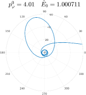
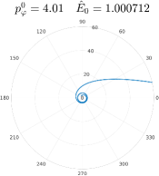
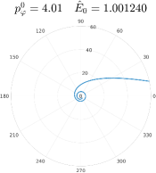
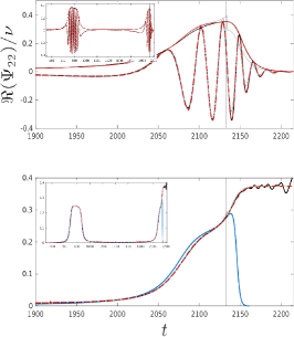
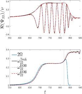
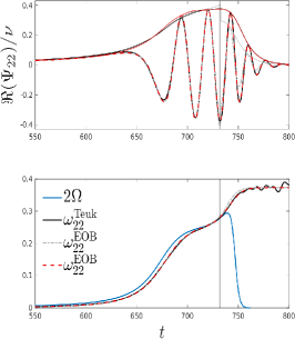
Figure 14: Upper panels: trajectories for nonspinning dynamical captures, with $\nu=10^{-2}$, $p_{\varphi}^{0}=4.01$, and $\hat{E}_{0}=\left(1.000711,1.000712,1.001240\right)$. The trajectories start from $r_{0}=120$, but we show them from $r=60$ in order to highlight the last part. Middle panels: corresponding quadrupolar waveforms. The black line is the numerical result from Teukode, while the red and grey lines are obtained with the EOB model using different prescriptions for the modelization of the ringdown. See text for more details. Bottom panels: frequency comparisons. The vertical lines mark the merger time (i.e. the peak of the $\ell=m=2$ waveform amplitude), that in the hyperbolic case is extracted directly from numerical data.

Recently, TEOBResumS has been generalized so to faithfully model also hyperbolic encounters and dynamical capture black hole binaries Nagar et al. (2021a, b). Nonetheless,the ringdown model used in these cases is the same adopted for quasi-circular waveforms, and it might be attached to the inspiral waveform without NQC corrections Gamba et al. (2021). Despite these simplifications, this model allowed for a robust interpretation of GW190521 Abbott et al. (2020) as the outcome of the dynamical capture of two black holes Gamba et al. (2021).

Since the test-particle limit provides a useful laboratory to test the EOB prescriptions, we will now focus on hyperbolic captures in the test-mass limit to discuss various ringdown implementation and complement the information given in Ref. Gamba et al. (2021). The EOB dynamics and waveforms of this section are obtained with the EOB model exposed above, using the angular radiation reaction of Eq. (22), that is also the one used for the analysis of GW190521 in Ref. Gamba et al. (2021). Nonetheless, the definitions of eccentricity and semilatus rectum provided in Eqs. (9) are no longer valid since the two radial turning points are not defined for unbound motion. Therefore, as in Ref. Nagar et al. (2021a), in this case we provide initial data to the dynamics directly providing the energy $\hat{E}_{0}$ and the angular momentum $p_{\varphi}^{0}$. Practically, we choose $p_{\varphi}^{0}$ and then pick $1<\hat{E}_{0}<\hat{E}^{\rm max}_{0}$, where $\hat{E}^{\rm max}_{0}$ is the square root of the peak of the Schwarzschild effective potential

$$V^{\rm Schw}_{\rm eff}=A(r)(1+p_{\varphi}^{2}u^{2}).$$ (51)

We choose this region of the parameter space because it is the one that yields the most interesting phenomenologies. In fact, for $\hat{E}_{0}>\hat{E}_{0}^{\rm max}$ there is always a direct plunge, while in the other case it is possible to have many close passages before merger. For example, choosing $\nu=10^{-2}$ and starting the dynamics at $r_{0}=120$ with $p_{\varphi}^{0}=4.08$ and $\hat{E}_{0}=1.00002$ leads to 11 close passages before merger.

It is not our aim here to carry out a systematic analysis of the parameter space as done for bound orbits, so we will only focus our discussion on a few, illustrative, cases. Moreover, while in Sec. V.2 we have considered $\nu=10^{-3}$, here we use $\nu=10^{-2}$. This makes the dynamics with multiple encounters shorter and the corresponding numerical waveforms require less computational time. This is not a big deal at the moment, since we want to specifically focus on the ringdown part. We consider three $\nu=10^{-2}$ configurations, with $r_{0}=120$, $p_{\varphi}^{0}=4.01$, and different values of energy: $\hat{E}_{0}=\left(1.000711,1.000712,1.001240\right)$ ($\hat{E}^{\rm max}_{0}\simeq 1.00125$). The first one is a double encounter, while the others are single encounters. The trajectories, the quadrupolar waveforms and the corresponding frequencies are shown in Fig. 14. The black waveform is as usual the numerical result, while on the analytical side we consider two different EOB waveforms colored in grey and red. The former is obtained attaching the circular ringdown to the analytical waveform, similarly to what is done for hyperbolic encounters in Refs. Nagar et al. (2021a, b), but without using NQC corrections as in Ref. Gamba et al. (2021). The primary templates for the phase and the amplitude used in Fig. 14 are the ones described in Sec. V.2. For the red waveform we consider the same templates, but we extract the fit parameters and the numerical quantities discussed in Sec. V.2 directly from the numerical waveforms. A similar use of the numerical data is also done to determine the NQC coefficients $(a_{i},b_{i})$ of Eq. (47). Finally, also the merger time $t_{\rm mrg}$ is taken to be precisely the numerical one, since the simple prescription $t_{\rm mrg}=t^{\rm peak}_{\Omega_{\rm orb}}-3$ used for bound orbits is found to be inaccurate in the hyperbolic case. In future work we plan a systematic campaign of simulations of hyperbolic encounters so to inform suitable analytical representations of both $t_{\rm mrg}$ and the ringdown parameters valid for any configurations, analogously to the case of bound orbits. In any case, as a proof of principle, the improvement introduced in the red waveform by the use of more precise parameters is clearly visible either before and after the merger. These comparisons show that including numerical information in the model from hyperbolic simulations could greatly enhance the analytical descriptions of waveforms emitted by the dynamical capture of two black holes. In particular, a systematic coverage of black hole binaries undergoing dynamical encounters using numerical relativity Gold and Brügmann (2013) will be instrumental to improve the waveform model TEOBResumS for these configurations Nagar et al. (2021a). This is expected to enhance the current analysis of GW190521 under the dynamical capture hypothesis Gamba et al. (2021).

VI Conclusions

In this paper we have analyzed in detail and improved the proposal of Chiaramello and Nagar (2020) for incorporating eccentricity effects within the EOB waveform and radiation reaction. We focused our analysis on the large mass ratio limit. We have tested the performance of the analytical prescription for the fluxes over a significant portion of the parameter space by comparing it with highly accurate waveforms and fluxes obtained solving numerically the Teukolsky equation using Teukode. We have strengthened the PN corrections to the waveform amplitude using a proper resummation of the ${\ell}=7$ and ${\ell}=8$ modes. We have also improved the residual phase of the tail factor introducing 7.5 PN information in the $\delta_{\ell m}$.

The advances introduced in this work provide an analytical EOB prescription for the waveform and fluxes that can be used in the description of EMRIs without the need of solving numerically the computationally-expensive Teukolsky equation. The analytical waveform is accurate over a large portion of the parameter space, as shown in Sec. V. Moreover, the systematic analysis of the fluxes of Sec. IV has shown that the radiation reaction is reliable with errors of the few percents for moderate eccentricities ($e\lesssim 0.3$) and spin-parameters not too high. In Sec. V.2, we have also shown a preliminary work for the complete EOB waveform, from inspiral to ringdown, that we will discuss in more detail in future studies. In Sec. V.3 we have also shown some hyperbolic encounters.

The work presented here should be seen as a first step toward modeling eccentric EMRIs within the EOB formalism, improving on previous work that was limited to quasi-circular configurations Yunes et al. (2011). Two immediate next steps will be considered in future work. (i) The inclusion of Gravitational Self-Force (GSF) results concerning the central EOB potentials, $(A,D,Q)$. Similar approaches have been proposed in other works Barausse et al. (2012b); Antonelli et al. (2020). It could be similarly implemented using using the Hamiltonian of TEOBResumS, that is a mass-ratio deformation of the one of a (spinning) test-particle around a Kerr black hole, where the 5PN resummed potentials are replaced by the corresponding one obtained from GSF knowledge Akcay and van de Meent (2016). Together with the radiation reaction discussed here, this analytical improvement would pave the way to a fully GSF-informed EOB model for eccentric EMRIs on equatorial orbits, analogously to NR-informed EOB models for coalescing black hole binaries. (ii) The fluxes and waveform will have to be improved incorporating additional PN information Mishra et al. (2015) beyond the Newtonian prefactors considered here. This will hopefully allow one to reduce the analytical/numerical differences that we found when eccentricities are large.

A GSF-faithful EOB model can be used to generate a wide bank of EMRI waveforms. It is however unlikely that the efficiency of the waveform generation will be sufficient for direct use in parameter estimation (see in particular discussion in Appendix C of Ref. Nagar et al. (2021b)). Nonetheless, these EOB templates can be used to create a fast and accurate surrogate using machine learning techniques, similarly to what has been done in Ref. Schmidt et al. (2021) for comparable mass binaries (up to mass ratio $q=20$). Such surrogate can then be employed for parameter estimation of EMRIs to be detected by LISA, as a complementary tool to other frameworks Katz et al. (2021); Hughes et al. (2021).

VII Acknowledgement

S. B. acknowledges support by the EU H2020 under ERC Starting Grant, no. BinGraSp-714626. The numerical simulations using Teukode were performed on the Virgo “Tullio” server in Torino, supported by INFN. We are grateful to S. Hughes for the numerical data behind Fig. 2 and to D. Chiaramello for the preliminary work on the analytical model of the ringdown and for the RWZhyp’s simulations used in Table 1 and Table 4.

Appendix A Circular EOB

A.1 Multipolar waveform factorization

In Eq. (14) we have recalled the multipolar factorization of the EOB waveform. Here we briefly expose the factors in more details, without assuming an high mass-ratio. The Newtonian factor for circularized binaries is explicitly given by

$$h_{{\ell m}}^{(N,\epsilon)}=\frac{M\nu}{D_{L}}n_{{\ell m}}^{(\epsilon)}c_{{\ell}+\epsilon}(\nu)x^{\frac{({\ell}+\epsilon)}{2}}Y^{{\ell}-\epsilon,-m}\left(\frac{\pi}{2},\varphi\right),$$ (52)

where $D_{L}$ is the luminosity distance, $x=\Omega^{2/3}$ and the coefficients are given by

$$n_{{\ell m}}^{(0)} =(im)^{{\ell}}\frac{8\pi}{(2{\ell}+1)!!}\sqrt{\frac{({\ell}+1)({\ell}+2)}{{\ell}({\ell}-1)}},$$

$$n_{{\ell m}}^{(1)} =-(im)^{{\ell}}\frac{16\pi i}{(2{\ell}+1)!!}\sqrt{\frac{(2{\ell}+1)({\ell}+2)\left({\ell}^{2}-m^{2}\right)}{(2{\ell}-1)({\ell}+1){\ell}({\ell}-1)}},$$

$$c_{{\ell}+\epsilon} =\left(\frac{m_{2}}{M}\right)^{{\ell}+\epsilon-1}+(-)^{{\ell}+\epsilon}\left(\frac{m_{1}}{M}\right)^{{\ell}+\epsilon-1}\mathrel{\mathop{=}\limits_{\nu\to 0}}\pm 1,$$

The factors of the PN correction $\hat{h}^{(\epsilon)}_{{\ell m}}$ are Damour and Nagar (2014a); Damour et al. (2009):

• the source term $\hat{S}_{\rm eff}^{(\epsilon)}$, whose expression depends on parity:

  $$\hat{S}_{\rm eff}^{(0)} ={\hat{H}^{\rm eq}_{\rm Kerr}},$$ (53a)

  $$\hat{S}_{\rm eff}^{(1)} =\frac{p_{\varphi}}{r_{\Omega}v_{\varphi}}.$$ (53b)

• the leading contribution of the tail factor $T_{{\ell m}}$, generated by the backscattering of the GWs with the Kerr background

  $$T_{{\ell m}}=\frac{\Gamma({\ell}+1-2ik)}{\Gamma\left({\ell}+1\right)}e^{\pi k}e^{2ik\ln\left(2kr_{0}\right)},$$

  where $k=m\Omega$, $r_{0}=2/\sqrt{e}$, and $\Gamma(z)$ is the Euler Gamma function.

• the residual phase of the tail factor $e^{i\delta_{{\ell m}}}$, that takes into account the fact that $T_{{\ell m}}$ includes only the leading contribution. We have analyzed these phases in Sec. III.4.

• the residual relativistic amplitude corrections $\rho_{{\ell m}}$, that are resummed following Refs. Nagar and Shah (2016); Messina et al. (2018). In Sec. III.3 we have extended this resummation scheme to ${\ell}=7$ and ${\ell}=8$.

In order to improve the agreement with numerical data during the plunge, it is useful to replace $x=\Omega^{2/3}$ with $x=r_{\Omega}^{2}\Omega^{2}\equiv v_{\varphi}^{2}$, where the spin-informed radius $r_{\Omega}$ is given by the third Kepler law generalized for circular orbits in Kerr spacetime Bardeen et al. (1972) (see Eq. (21)). The new $x$-parameter is more reliable for noncircular motion and it is used both in the Newtonian prefactors $h_{{\ell m}}^{(N,\epsilon)}$ and in the amplitude corrections $\rho_{\ell m}(x)$.

A.2 Angular radiation reaction

In the circular case, Eq. (19) reduces to

$$\dot{J} =-{\cal F}_{\varphi},$$

$$\dot{E} =\Omega\dot{J}.$$

Decomposing the energy in multipoles, we have

$$\dot{J}=\frac{1}{\Omega}\sum_{{\ell}=2}^{\infty}\sum_{m=1}^{{\ell}}F_{{\ell m}} =\frac{2}{16\pi\Omega}\sum_{{\ell}=2}^{\infty}\sum_{m=1}^{{\ell}}|\dot{h}_{{\ell m}}|^{2}$$

$$=\frac{1}{8\pi}\sum_{{\ell}=2}^{\infty}\sum_{m=1}^{{\ell}}m^{2}\Omega|h_{{\ell m}}|^{2},$$

then factorizing the Newtonian $(2,2)$ contribution, we can write the angular radiation reaction as

$$\hat{{\cal F}}_{\varphi}=-\frac{\dot{J}}{\nu}=-\frac{32}{5}\nu x^{7/2}\hat{f},$$ (54)

where

$$\hat{f} =\sum_{{\ell}=2}^{\infty}\sum_{m=1}^{{\ell}}(F_{22}^{N})^{-1}F_{{\ell m}}=\sum_{{\ell}=2}^{\infty}\sum_{m=1}^{{\ell}}\hat{F}_{\ell m},$$ (55)

$$F_{\ell m} =\frac{1}{8\pi}m^{2}\Omega^{2}|h_{{\ell m}}|^{2},$$ (56)

$$F_{22}^{N} =\frac{32}{5}x^{5}.$$ (57)

Finally, we can use the third Kepler law generalized to Kerr spacetime ($r_{\Omega}^{3}\Omega^{2}=1$) to write Eq. (20).

Appendix B Newtonian noncircular expressions

In Sec. III we have discussed the Newtonian noncircular corrections to the waveform, $\hat{h}_{{\ell m}}^{(N,\epsilon)_{\rm nc}}$, and the noncircular Newtonian prefactors for the angular radiation reaction, ${\hat{f}_{\varphi,{\ell m}}^{\rm N_{nc}}}$. Here we report them explicitly for the $({\ell},m)=(2,2),(2,1),(3,3),(3,2),(4,4)$ multipoles:

$$\hat{h}_{22}^{(N,0)_{\rm nc}}=1 -\frac{\dot{r}^{2}}{2r^{2}\Omega^{2}}-\frac{\ddot{r}}{2r\Omega^{2}}+i\left(\frac{2\dot{r}}{r\Omega}+\frac{{\dot{\Omega}}}{2\Omega^{2}}\right),$$

$$\hat{h}_{21}^{(N,1)_{\rm nc}}=1 -\frac{6\dot{r}^{2}}{r^{2}\Omega^{2}}-\frac{3\ddot{r}}{r\Omega^{2}}-\frac{6\dot{r}{\dot{\Omega}}}{r\Omega^{3}}-\frac{{\ddot{\Omega}}}{\Omega^{3}}+i\left(\frac{6\dot{r}}{r\Omega}+\frac{3{\dot{\Omega}}}{\Omega^{2}}\right),$$

$$\hat{h}_{33}^{(N,0)_{\rm nc}}=1 -\frac{2\dot{r}^{2}}{r^{2}\Omega^{2}}-\frac{\ddot{r}}{r\Omega^{2}}-\frac{\dot{r}{\dot{\Omega}}}{r\Omega^{3}}-\frac{{\ddot{\Omega}}}{9\Omega^{3}}+i\left(-\frac{2\dot{r}^{3}}{9r^{3}\Omega^{3}}-\frac{2\ddot{r}\dot{r}}{3r^{2}\Omega^{3}}-\frac{{r^{(3)}}}{9r\Omega^{3}}+\frac{3\dot{r}}{r\Omega}+\frac{{\dot{\Omega}}}{\Omega^{2}}\right),$$

$$\hat{h}_{32}^{(N,1)_{\rm nc}}=1 -\frac{9\dot{r}^{2}}{r^{2}\Omega^{2}}-\frac{3\ddot{r}}{r\Omega^{2}}-\frac{9\dot{r}{\dot{\Omega}}}{r\Omega^{3}}-\frac{3{\dot{\Omega}}^{2}}{4\Omega^{4}}-\frac{{\ddot{\Omega}}}{\Omega^{3}}+i\left(-\frac{3\dot{r}^{3}}{r^{3}\Omega^{3}}-\frac{9\ddot{r}\dot{r}}{2r^{2}\Omega^{3}}-\frac{9\dot{r}^{2}{\dot{\Omega}}}{2r^{2}\Omega^{4}}-\frac{3\ddot{r}{\dot{\Omega}}}{2r\Omega^{4}}\right.$$

$$\left.-\frac{{r^{(3)}}}{2r\Omega^{3}}-\frac{3\dot{r}{\ddot{\Omega}}}{2r\Omega^{4}}+\frac{6\dot{r}}{r\Omega}-\frac{{\Omega^{(3)}}}{8\Omega^{4}}+\frac{3{\dot{\Omega}}}{\Omega^{2}}\right),$$

$$\hat{h}_{44}^{(N,0)_{\rm nc}}=1 +\frac{3\dot{r}^{4}}{32r^{4}\Omega^{4}}+\frac{9\ddot{r}\dot{r}^{2}}{16r^{3}\Omega^{4}}+\frac{9\ddot{r}^{2}}{64r^{2}\Omega^{4}}+\frac{3{r^{(3)}}\dot{r}}{16r^{2}\Omega^{4}}-\frac{9\dot{r}^{2}}{2r^{2}\Omega^{2}}-\frac{3\ddot{r}}{2r\Omega^{2}}+\frac{{r^{(4)}}}{64r\Omega^{4}}-\frac{3\dot{r}{\dot{\Omega}}}{r\Omega^{3}}-\frac{3{\dot{\Omega}}^{2}}{16\Omega^{4}}$$

$$-\frac{{\ddot{\Omega}}}{4\Omega^{3}}+i\left(-\frac{3\dot{r}^{3}}{2r^{3}\Omega^{3}}-\frac{9\ddot{r}\dot{r}}{4r^{2}\Omega^{3}}-\frac{9\dot{r}^{2}{\dot{\Omega}}}{8r^{2}\Omega^{4}}-\frac{3\ddot{r}{\dot{\Omega}}}{8r\Omega^{4}}-\frac{{r^{(3)}}}{4r\Omega^{3}}-\frac{\dot{r}{\ddot{\Omega}}}{4r\Omega^{4}}+\frac{4\dot{r}}{r\Omega}-\frac{{\Omega^{(3)}}}{64\Omega^{4}}+\frac{3{\dot{\Omega}}}{2\Omega^{2}}\right),$$

$${\hat{f}_{\varphi,22}^{\rm N_{nc}}}=1 +\frac{3\dot{r}^{4}}{4r^{4}\Omega^{4}}+\frac{3\dot{r}^{3}{\dot{\Omega}}}{4r^{3}\Omega^{5}}+\frac{3\ddot{r}^{2}}{4r^{2}\Omega^{4}}+\frac{3\ddot{r}\dot{r}{\dot{\Omega}}}{8r^{2}\Omega^{5}}-\frac{{r^{(3)}}\dot{r}}{2r^{2}\Omega^{4}}+\frac{\dot{r}^{2}{\ddot{\Omega}}}{8r^{2}\Omega^{5}}+\frac{4\dot{r}^{2}}{r^{2}\Omega^{2}}+\frac{\ddot{r}{\ddot{\Omega}}}{8r\Omega^{5}}-\frac{2\ddot{r}}{r\Omega^{2}}$$

$$-\frac{{r^{(3)}}{\dot{\Omega}}}{8r\Omega^{5}}+\frac{3\dot{r}{\dot{\Omega}}}{r\Omega^{3}}+\frac{3{\dot{\Omega}}^{2}}{4\Omega^{4}}-\frac{{\ddot{\Omega}}}{4\Omega^{3}},$$

$${\hat{f}_{\varphi,21}^{\rm N_{nc}}}=1 +\frac{72\dot{r}^{4}}{r^{4}\Omega^{4}}+\frac{144\dot{r}^{3}{\dot{\Omega}}}{r^{3}\Omega^{5}}+\frac{27\ddot{r}^{2}}{r^{2}\Omega^{4}}+\frac{27\ddot{r}\dot{r}{\dot{\Omega}}}{r^{2}\Omega^{5}}-\frac{18{r^{(3)}}\dot{r}}{r^{2}\Omega^{4}}+\frac{126\dot{r}^{2}{\dot{\Omega}}^{2}}{r^{2}\Omega^{6}}-\frac{12\dot{r}^{2}{\ddot{\Omega}}}{r^{2}\Omega^{5}}+\frac{30\dot{r}^{2}}{r^{2}\Omega^{2}}-\frac{18\ddot{r}{\dot{\Omega}}^{2}}{r\Omega^{6}}$$

$$+\frac{21\ddot{r}{\ddot{\Omega}}}{r\Omega^{5}}-\frac{12\ddot{r}}{r\Omega^{2}}-\frac{9{r^{(3)}}{\dot{\Omega}}}{r\Omega^{5}}+\frac{18\dot{r}{\dot{\Omega}}^{3}}{r\Omega^{7}}+\frac{24\dot{r}{\ddot{\Omega}}{\dot{\Omega}}}{r\Omega^{6}}-\frac{6\dot{r}{\Omega^{(3)}}}{r\Omega^{5}}+\frac{30\dot{r}{\dot{\Omega}}}{r\Omega^{3}}+\frac{3{\ddot{\Omega}}{\dot{\Omega}}^{2}}{\Omega^{7}}+\frac{4{\ddot{\Omega}}^{2}}{\Omega^{6}}$$

$$-\frac{3{\Omega^{(3)}}{\dot{\Omega}}}{\Omega^{6}}+\frac{15{\dot{\Omega}}^{2}}{\Omega^{4}}-\frac{5{\ddot{\Omega}}}{\Omega^{3}},$$

$${\hat{f}_{\varphi,33}^{\rm N_{nc}}}=1 +\frac{16\dot{r}^{6}}{81r^{6}\Omega^{6}}+\frac{8\ddot{r}\dot{r}^{4}}{27r^{5}\Omega^{6}}+\frac{8\dot{r}^{5}{\dot{\Omega}}}{27r^{5}\Omega^{7}}+\frac{8\ddot{r}^{2}\dot{r}^{2}}{9r^{4}\Omega^{6}}+\frac{16\ddot{r}\dot{r}^{3}{\dot{\Omega}}}{27r^{4}\Omega^{7}}-\frac{32{r^{(3)}}\dot{r}^{3}}{81r^{4}\Omega^{6}}+\frac{8\dot{r}^{4}{\ddot{\Omega}}}{81r^{4}\Omega^{7}}+\frac{40\dot{r}^{4}}{9r^{4}\Omega^{4}}-\frac{2\ddot{r}^{3}}{9r^{3}\Omega^{6}}$$

$$+\frac{2\ddot{r}^{2}\dot{r}{\dot{\Omega}}}{9r^{3}\Omega^{7}}+\frac{8\ddot{r}{r^{(3)}}\dot{r}}{27r^{3}\Omega^{6}}+\frac{20\ddot{r}\dot{r}^{2}{\ddot{\Omega}}}{81r^{3}\Omega^{7}}-\frac{20\ddot{r}\dot{r}^{2}}{9r^{3}\Omega^{4}}-\frac{4{r^{(3)}}\dot{r}^{2}{\dot{\Omega}}}{27r^{3}\Omega^{7}}-\frac{2{r^{(4)}}\dot{r}^{2}}{27r^{3}\Omega^{6}}+\frac{2\dot{r}^{3}{\Omega^{(3)}}}{243r^{3}\Omega^{7}}+\frac{20\dot{r}^{3}{\dot{\Omega}}}{3r^{3}\Omega^{5}}-\frac{2\ddot{r}^{2}{\ddot{\Omega}}}{81r^{2}\Omega^{7}}$$

$$+\frac{20\ddot{r}^{2}}{9r^{2}\Omega^{4}}+\frac{2\ddot{r}{r^{(3)}}{\dot{\Omega}}}{27r^{2}\Omega^{7}}-\frac{\ddot{r}{r^{(4)}}}{27r^{2}\Omega^{6}}+\frac{2\ddot{r}\dot{r}{\Omega^{(3)}}}{81r^{2}\Omega^{7}}+\frac{4{r^{(3)}}^{2}}{81r^{2}\Omega^{6}}+\frac{4{r^{(3)}}\dot{r}{\ddot{\Omega}}}{243r^{2}\Omega^{7}}-\frac{40{r^{(3)}}\dot{r}}{27r^{2}\Omega^{4}}-\frac{{r^{(4)}}\dot{r}{\dot{\Omega}}}{27r^{2}\Omega^{7}}+\frac{10\dot{r}^{2}{\dot{\Omega}}^{2}}{3r^{2}\Omega^{6}}$$

$$+\frac{6\dot{r}^{2}}{r^{2}\Omega^{2}}-\frac{\ddot{r}{\dot{\Omega}}^{2}}{3r\Omega^{6}}+\frac{2\ddot{r}{\ddot{\Omega}}}{3r\Omega^{5}}-\frac{3\ddot{r}}{r\Omega^{2}}+\frac{{r^{(3)}}{\Omega^{(3)}}}{243r\Omega^{7}}-\frac{2{r^{(3)}}{\dot{\Omega}}}{3r\Omega^{5}}-\frac{{r^{(4)}}{\ddot{\Omega}}}{243r\Omega^{7}}+\frac{{r^{(4)}}}{27r\Omega^{4}}+\frac{\dot{r}{\dot{\Omega}}^{3}}{3r\Omega^{7}}$$

$$+\frac{4\dot{r}{\ddot{\Omega}}{\dot{\Omega}}}{9r\Omega^{6}}-\frac{\dot{r}{\Omega^{(3)}}}{9r\Omega^{5}}+\frac{5\dot{r}{\dot{\Omega}}}{r\Omega^{3}}+\frac{{\ddot{\Omega}}{\dot{\Omega}}^{2}}{27\Omega^{7}}+\frac{4{\ddot{\Omega}}^{2}}{81\Omega^{6}}-\frac{{\Omega^{(3)}}{\dot{\Omega}}}{27\Omega^{6}}+\frac{5{\dot{\Omega}}^{2}}{3\Omega^{4}}-\frac{5{\ddot{\Omega}}}{9\Omega^{3}},$$

$${\hat{f}_{\varphi,32}^{\rm N_{nc}}}=1 +\frac{45\dot{r}^{6}}{2r^{6}\Omega^{6}}+\frac{135{\dot{\Omega}}\dot{r}^{5}}{2r^{5}\Omega^{7}}+\frac{675{\dot{\Omega}}^{2}\dot{r}^{4}}{8r^{4}\Omega^{8}}+\frac{135\dot{r}^{4}}{2r^{4}\Omega^{4}}+\frac{45\ddot{r}\dot{r}^{4}}{2r^{5}\Omega^{6}}+\frac{45{\dot{\Omega}}^{3}\dot{r}^{3}}{2r^{3}\Omega^{9}}-\frac{45{\Omega^{(3)}}\dot{r}^{3}}{8r^{3}\Omega^{7}}+\frac{135{\ddot{\Omega}}{\dot{\Omega}}\dot{r}^{3}}{4r^{3}\Omega^{8}}$$

$$+\frac{135{\dot{\Omega}}\dot{r}^{3}}{r^{3}\Omega^{5}}+\frac{135\ddot{r}{\dot{\Omega}}\dot{r}^{3}}{2r^{4}\Omega^{7}}-\frac{15{r^{(3)}}\dot{r}^{3}}{r^{4}\Omega^{6}}+\frac{15{\ddot{\Omega}}^{2}\dot{r}^{2}}{2r^{2}\Omega^{8}}+\frac{45{\ddot{\Omega}}{\dot{\Omega}}^{2}\dot{r}^{2}}{4r^{2}\Omega^{9}}+\frac{495{\dot{\Omega}}^{2}\dot{r}^{2}}{4r^{2}\Omega^{6}}+\frac{81\ddot{r}{\dot{\Omega}}^{2}\dot{r}^{2}}{4r^{3}\Omega^{8}}-\frac{15{\ddot{\Omega}}\dot{r}^{2}}{r^{2}\Omega^{5}}$$

$$+\frac{27\ddot{r}{\ddot{\Omega}}\dot{r}^{2}}{r^{3}\Omega^{7}}-\frac{9{\Omega^{(4)}}\dot{r}^{2}}{16r^{2}\Omega^{7}}-\frac{45{\Omega^{(3)}}{\dot{\Omega}}\dot{r}^{2}}{16r^{2}\Omega^{8}}-\frac{27{r^{(3)}}{\dot{\Omega}}\dot{r}^{2}}{2r^{3}\Omega^{7}}+\frac{21\dot{r}^{2}}{r^{2}\Omega^{2}}-\frac{27\ddot{r}\dot{r}^{2}}{r^{3}\Omega^{4}}+\frac{135\ddot{r}^{2}\dot{r}^{2}}{4r^{4}\Omega^{6}}-\frac{9{r^{(4)}}\dot{r}^{2}}{4r^{3}\Omega^{6}}$$

$$+\frac{135{\dot{\Omega}}^{3}\dot{r}}{4r\Omega^{7}}+\frac{9\ddot{r}{\dot{\Omega}}^{3}\dot{r}}{4r^{2}\Omega^{9}}-\frac{33{r^{(3)}}{\dot{\Omega}}^{2}\dot{r}}{4r^{2}\Omega^{8}}+\frac{4{r^{(3)}}{\ddot{\Omega}}\dot{r}}{r^{2}\Omega^{7}}+\frac{15{\ddot{\Omega}}{\Omega^{(3)}}\dot{r}}{16r\Omega^{8}}-\frac{15{\Omega^{(3)}}\dot{r}}{4r\Omega^{5}}+\frac{33\ddot{r}{\Omega^{(3)}}\dot{r}}{16r^{2}\Omega^{7}}+\frac{15{\ddot{\Omega}}^{2}{\dot{\Omega}}\dot{r}}{8r\Omega^{9}}$$

$$+\frac{15{\ddot{\Omega}}{\dot{\Omega}}\dot{r}}{2r\Omega^{6}}+\frac{69\ddot{r}{\ddot{\Omega}}{\dot{\Omega}}\dot{r}}{8r^{2}\Omega^{8}}-\frac{9{\Omega^{(4)}}{\dot{\Omega}}\dot{r}}{16r\Omega^{8}}+\frac{21{\dot{\Omega}}\dot{r}}{r\Omega^{3}}-\frac{15\ddot{r}{\dot{\Omega}}\dot{r}}{2r^{2}\Omega^{5}}+\frac{81\ddot{r}^{2}{\dot{\Omega}}\dot{r}}{4r^{3}\Omega^{7}}-\frac{9{r^{(4)}}{\dot{\Omega}}\dot{r}}{4r^{2}\Omega^{7}}-\frac{13{r^{(3)}}\dot{r}}{r^{2}\Omega^{4}}$$

$$+\frac{9\ddot{r}{r^{(3)}}\dot{r}}{r^{3}\Omega^{6}}+\frac{45{\dot{\Omega}}^{4}}{16\Omega^{8}}-\frac{3{r^{(3)}}{\dot{\Omega}}^{3}}{4r\Omega^{9}}+\frac{5{\ddot{\Omega}}^{2}}{2\Omega^{6}}-\frac{3\ddot{r}{\ddot{\Omega}}^{2}}{2r\Omega^{8}}+\frac{5{\Omega^{(3)}}^{2}}{64\Omega^{8}}+\frac{15{\ddot{\Omega}}{\dot{\Omega}}^{2}}{8\Omega^{7}}+\frac{3\ddot{r}{\ddot{\Omega}}{\dot{\Omega}}^{2}}{4r\Omega^{9}}$$

$$-\frac{3{\Omega^{(4)}}{\dot{\Omega}}^{2}}{64\Omega^{9}}+\frac{21{\dot{\Omega}}^{2}}{2\Omega^{4}}-\frac{75\ddot{r}{\dot{\Omega}}^{2}}{4r\Omega^{6}}+\frac{189\ddot{r}^{2}{\dot{\Omega}}^{2}}{16r^{2}\Omega^{8}}-\frac{3{r^{(4)}}{\dot{\Omega}}^{2}}{16r\Omega^{8}}-\frac{7{\ddot{\Omega}}}{2\Omega^{3}}+\frac{15\ddot{r}{\ddot{\Omega}}}{r\Omega^{5}}-\frac{27\ddot{r}^{2}{\ddot{\Omega}}}{4r^{2}\Omega^{7}}$$

$$-\frac{{r^{(4)}}{\ddot{\Omega}}}{4r\Omega^{7}}+\frac{9{r^{(3)}}{\Omega^{(3)}}}{16r\Omega^{7}}-\frac{{\ddot{\Omega}}{\Omega^{(4)}}}{16\Omega^{8}}+\frac{{\Omega^{(4)}}}{16\Omega^{5}}-\frac{3\ddot{r}{\Omega^{(4)}}}{16r\Omega^{7}}-\frac{3{r^{(3)}}{\ddot{\Omega}}{\dot{\Omega}}}{8r\Omega^{8}}+\frac{5{\ddot{\Omega}}{\Omega^{(3)}}{\dot{\Omega}}}{32\Omega^{9}}-\frac{5{\Omega^{(3)}}{\dot{\Omega}}}{2\Omega^{6}}$$

$$+\frac{33\ddot{r}{\Omega^{(3)}}{\dot{\Omega}}}{16r\Omega^{8}}-\frac{15{r^{(3)}}{\dot{\Omega}}}{2r\Omega^{5}}+\frac{9\ddot{r}{r^{(3)}}{\dot{\Omega}}}{2r^{2}\Omega^{7}}-\frac{9\ddot{r}}{r\Omega^{2}}+\frac{81\ddot{r}^{2}}{4r^{2}\Omega^{4}}+\frac{{r^{(4)}}}{4r\Omega^{4}}-\frac{27\ddot{r}^{3}}{4r^{3}\Omega^{6}}+\frac{{r^{(3)}}^{2}}{r^{2}\Omega^{6}}-\frac{3\ddot{r}{r^{(4)}}}{4r^{2}\Omega^{6}},$$

$${\hat{f}_{\varphi,44}^{\rm N_{nc}}}=1 +\frac{45\dot{r}^{8}}{1024r^{8}\Omega^{8}}+\frac{45{\dot{\Omega}}\dot{r}^{7}}{512r^{7}\Omega^{9}}+\frac{45{\ddot{\Omega}}\dot{r}^{6}}{1024r^{6}\Omega^{9}}+\frac{45\dot{r}^{6}}{16r^{6}\Omega^{6}}+\frac{45\ddot{r}\dot{r}^{6}}{256r^{7}\Omega^{8}}+\frac{15{\Omega^{(3)}}\dot{r}^{5}}{2048r^{5}\Omega^{9}}+\frac{405{\dot{\Omega}}\dot{r}^{5}}{64r^{5}\Omega^{7}}$$

$$+\frac{405\ddot{r}{\dot{\Omega}}\dot{r}^{5}}{1024r^{6}\Omega^{9}}-\frac{45{r^{(3)}}\dot{r}^{5}}{256r^{6}\Omega^{8}}+\frac{1215{\dot{\Omega}}^{2}\dot{r}^{4}}{256r^{4}\Omega^{8}}+\frac{135{\ddot{\Omega}}\dot{r}^{4}}{256r^{4}\Omega^{7}}+\frac{225\ddot{r}{\ddot{\Omega}}\dot{r}^{4}}{1024r^{5}\Omega^{9}}+\frac{3{\Omega^{(4)}}\dot{r}^{4}}{8192r^{4}\Omega^{9}}-\frac{75{r^{(3)}}{\dot{\Omega}}\dot{r}^{4}}{1024r^{5}\Omega^{9}}$$

$$+\frac{189\dot{r}^{4}}{16r^{4}\Omega^{4}}+\frac{675\ddot{r}^{2}\dot{r}^{4}}{1024r^{6}\Omega^{8}}-\frac{75{r^{(4)}}\dot{r}^{4}}{1024r^{5}\Omega^{8}}+\frac{225{\dot{\Omega}}^{3}\dot{r}^{3}}{256r^{3}\Omega^{9}}+\frac{15{r^{(3)}}{\ddot{\Omega}}\dot{r}^{3}}{512r^{4}\Omega^{9}}-\frac{45{\Omega^{(3)}}\dot{r}^{3}}{256r^{3}\Omega^{7}}+\frac{165\ddot{r}{\Omega^{(3)}}\dot{r}^{3}}{4096r^{4}\Omega^{9}}$$

$$+\frac{45{\ddot{\Omega}}{\dot{\Omega}}\dot{r}^{3}}{32r^{3}\Omega^{8}}+\frac{315{\dot{\Omega}}\dot{r}^{3}}{16r^{3}\Omega^{5}}+\frac{405\ddot{r}{\dot{\Omega}}\dot{r}^{3}}{128r^{4}\Omega^{7}}+\frac{225\ddot{r}^{2}{\dot{\Omega}}\dot{r}^{3}}{512r^{5}\Omega^{9}}-\frac{105{r^{(4)}}{\dot{\Omega}}\dot{r}^{3}}{2048r^{4}\Omega^{9}}-\frac{45{r^{(3)}}\dot{r}^{3}}{16r^{4}\Omega^{6}}+\frac{75\ddot{r}{r^{(3)}}\dot{r}^{3}}{256r^{5}\Omega^{8}}$$

$$-\frac{3{r^{(5)}}\dot{r}^{3}}{512r^{4}\Omega^{8}}+\frac{25{\ddot{\Omega}}^{2}\dot{r}^{2}}{128r^{2}\Omega^{8}}+\frac{165{\ddot{\Omega}}{\dot{\Omega}}^{2}\dot{r}^{2}}{512r^{2}\Omega^{9}}+\frac{105{\dot{\Omega}}^{2}\dot{r}^{2}}{8r^{2}\Omega^{6}}+\frac{135\ddot{r}{\dot{\Omega}}^{2}\dot{r}^{2}}{128r^{3}\Omega^{8}}-\frac{35{\ddot{\Omega}}\dot{r}^{2}}{32r^{2}\Omega^{5}}+\frac{225\ddot{r}{\ddot{\Omega}}\dot{r}^{2}}{128r^{3}\Omega^{7}}$$

$$+\frac{135\ddot{r}^{2}{\ddot{\Omega}}\dot{r}^{2}}{2048r^{4}\Omega^{9}}-\frac{15{r^{(4)}}{\ddot{\Omega}}\dot{r}^{2}}{2048r^{3}\Omega^{9}}+\frac{45{r^{(3)}}{\Omega^{(3)}}\dot{r}^{2}}{4096r^{3}\Omega^{9}}-\frac{9{\Omega^{(4)}}\dot{r}^{2}}{512r^{2}\Omega^{7}}+\frac{9\ddot{r}{\Omega^{(4)}}\dot{r}^{2}}{4096r^{3}\Omega^{9}}-\frac{15{\Omega^{(3)}}{\dot{\Omega}}\dot{r}^{2}}{256r^{2}\Omega^{8}}-\frac{315{r^{(3)}}{\dot{\Omega}}\dot{r}^{2}}{128r^{3}\Omega^{7}}$$

$$+\frac{135\ddot{r}{r^{(3)}}{\dot{\Omega}}\dot{r}^{2}}{1024r^{4}\Omega^{9}}-\frac{9{r^{(5)}}{\dot{\Omega}}\dot{r}^{2}}{2048r^{3}\Omega^{9}}+\frac{8\dot{r}^{2}}{r^{2}\Omega^{2}}-\frac{63\ddot{r}\dot{r}^{2}}{8r^{3}\Omega^{4}}+\frac{135\ddot{r}^{2}\dot{r}^{2}}{32r^{4}\Omega^{6}}-\frac{15{r^{(4)}}\dot{r}^{2}}{64r^{3}\Omega^{6}}+\frac{15{r^{(3)}}^{2}\dot{r}^{2}}{128r^{4}\Omega^{8}}$$

$$-\frac{45\ddot{r}{r^{(4)}}\dot{r}^{2}}{1024r^{4}\Omega^{8}}+\frac{45{\dot{\Omega}}^{3}\dot{r}}{16r\Omega^{7}}+\frac{45\ddot{r}{\dot{\Omega}}^{3}\dot{r}}{512r^{2}\Omega^{9}}-\frac{75{r^{(3)}}{\dot{\Omega}}^{2}\dot{r}}{128r^{2}\Omega^{8}}+\frac{15{r^{(3)}}{\ddot{\Omega}}\dot{r}}{128r^{2}\Omega^{7}}-\frac{{r^{(5)}}{\ddot{\Omega}}\dot{r}}{1024r^{2}\Omega^{9}}+\frac{5{\ddot{\Omega}}{\Omega^{(3)}}\dot{r}}{256r\Omega^{8}}$$

$$-\frac{5{\Omega^{(3)}}\dot{r}}{16r\Omega^{5}}+\frac{75\ddot{r}{\Omega^{(3)}}\dot{r}}{512r^{2}\Omega^{7}}+\frac{45\ddot{r}^{2}{\Omega^{(3)}}\dot{r}}{8192r^{3}\Omega^{9}}+\frac{5{r^{(4)}}{\Omega^{(3)}}\dot{r}}{16384r^{2}\Omega^{9}}+\frac{3{r^{(3)}}{\Omega^{(4)}}\dot{r}}{4096r^{2}\Omega^{9}}+\frac{5{\ddot{\Omega}}^{2}{\dot{\Omega}}\dot{r}}{128r\Omega^{9}}+\frac{5{\ddot{\Omega}}{\dot{\Omega}}\dot{r}}{8r\Omega^{6}}$$

$$+\frac{15\ddot{r}{\ddot{\Omega}}{\dot{\Omega}}\dot{r}}{32r^{2}\Omega^{8}}-\frac{3{\Omega^{(4)}}{\dot{\Omega}}\dot{r}}{256r\Omega^{8}}+\frac{7{\dot{\Omega}}\dot{r}}{r\Omega^{3}}-\frac{105\ddot{r}{\dot{\Omega}}\dot{r}}{32r^{2}\Omega^{5}}+\frac{405\ddot{r}^{2}{\dot{\Omega}}\dot{r}}{256r^{3}\Omega^{7}}-\frac{135{r^{(4)}}{\dot{\Omega}}\dot{r}}{512r^{2}\Omega^{7}}+\frac{135\ddot{r}^{3}{\dot{\Omega}}\dot{r}}{2048r^{4}\Omega^{9}}$$

$$+\frac{15{r^{(3)}}^{2}{\dot{\Omega}}\dot{r}}{512r^{3}\Omega^{9}}-\frac{21{r^{(3)}}\dot{r}}{8r^{2}\Omega^{4}}+\frac{45\ddot{r}{r^{(3)}}\dot{r}}{32r^{3}\Omega^{6}}+\frac{{r^{(5)}}\dot{r}}{64r^{2}\Omega^{6}}-\frac{45\ddot{r}^{2}{r^{(3)}}\dot{r}}{512r^{4}\Omega^{8}}+\frac{15{r^{(3)}}{r^{(4)}}\dot{r}}{1024r^{3}\Omega^{8}}-\frac{9\ddot{r}{r^{(5)}}\dot{r}}{1024r^{3}\Omega^{8}}$$

$$+\frac{45{\dot{\Omega}}^{4}}{256\Omega^{8}}-\frac{15{r^{(3)}}{\dot{\Omega}}^{3}}{512r\Omega^{9}}+\frac{5{\ddot{\Omega}}^{2}}{32\Omega^{6}}-\frac{5\ddot{r}{\ddot{\Omega}}^{2}}{128r\Omega^{8}}+\frac{5{\Omega^{(3)}}^{2}}{4096\Omega^{8}}+\frac{15{\ddot{\Omega}}{\dot{\Omega}}^{2}}{128\Omega^{7}}+\frac{15\ddot{r}{\ddot{\Omega}}{\dot{\Omega}}^{2}}{512r\Omega^{9}}$$

$$-\frac{3{\Omega^{(4)}}{\dot{\Omega}}^{2}}{4096\Omega^{9}}+\frac{21{\dot{\Omega}}^{2}}{8\Omega^{4}}-\frac{15\ddot{r}{\dot{\Omega}}^{2}}{8r\Omega^{6}}+\frac{225\ddot{r}^{2}{\dot{\Omega}}^{2}}{512r^{2}\Omega^{8}}-\frac{15{r^{(4)}}{\dot{\Omega}}^{2}}{512r\Omega^{8}}-\frac{7{\ddot{\Omega}}}{8\Omega^{3}}+\frac{55\ddot{r}{\ddot{\Omega}}}{32r\Omega^{5}}$$

$$-\frac{255\ddot{r}^{2}{\ddot{\Omega}}}{512r^{2}\Omega^{7}}-\frac{15{r^{(4)}}{\ddot{\Omega}}}{512r\Omega^{7}}+\frac{45\ddot{r}^{3}{\ddot{\Omega}}}{2048r^{3}\Omega^{9}}+\frac{5\ddot{r}{r^{(4)}}{\ddot{\Omega}}}{2048r^{2}\Omega^{9}}+\frac{15{r^{(3)}}{\Omega^{(3)}}}{512r\Omega^{7}}-\frac{15\ddot{r}{r^{(3)}}{\Omega^{(3)}}}{8192r^{2}\Omega^{9}}-\frac{{r^{(5)}}{\Omega^{(3)}}}{16384r\Omega^{9}}$$

$$-\frac{{\ddot{\Omega}}{\Omega^{(4)}}}{1024\Omega^{8}}+\frac{{\Omega^{(4)}}}{256\Omega^{5}}-\frac{3\ddot{r}{\Omega^{(4)}}}{512r\Omega^{7}}+\frac{9\ddot{r}^{2}{\Omega^{(4)}}}{16384r^{2}\Omega^{9}}+\frac{{r^{(4)}}{\Omega^{(4)}}}{16384r\Omega^{9}}+\frac{5{\ddot{\Omega}}{\Omega^{(3)}}{\dot{\Omega}}}{2048\Omega^{9}}-\frac{5{\Omega^{(3)}}{\dot{\Omega}}}{32\Omega^{6}}$$

$$+\frac{15\ddot{r}{\Omega^{(3)}}{\dot{\Omega}}}{256r\Omega^{8}}-\frac{45{r^{(3)}}{\dot{\Omega}}}{32r\Omega^{5}}+\frac{165\ddot{r}{r^{(3)}}{\dot{\Omega}}}{256r^{2}\Omega^{7}}+\frac{3{r^{(5)}}{\dot{\Omega}}}{512r\Omega^{7}}-\frac{45\ddot{r}^{2}{r^{(3)}}{\dot{\Omega}}}{2048r^{3}\Omega^{9}}+\frac{5{r^{(3)}}{r^{(4)}}{\dot{\Omega}}}{2048r^{2}\Omega^{9}}-\frac{3\ddot{r}{r^{(5)}}{\dot{\Omega}}}{2048r^{2}\Omega^{9}}$$

$$-\frac{4\ddot{r}}{r\Omega^{2}}+\frac{147\ddot{r}^{2}}{32r^{2}\Omega^{4}}+\frac{3{r^{(4)}}}{32r\Omega^{4}}-\frac{45\ddot{r}^{3}}{32r^{3}\Omega^{6}}+\frac{5{r^{(3)}}^{2}}{32r^{2}\Omega^{6}}-\frac{5\ddot{r}{r^{(4)}}}{32r^{2}\Omega^{6}}+\frac{405\ddot{r}^{4}}{4096r^{4}\Omega^{8}}$$

$$-\frac{15\ddot{r}{r^{(3)}}^{2}}{512r^{3}\Omega^{8}}+\frac{5{r^{(4)}}^{2}}{4096r^{2}\Omega^{8}}+\frac{45\ddot{r}^{2}{r^{(4)}}}{2048r^{3}\Omega^{8}}-\frac{{r^{(3)}}{r^{(5)}}}{1024r^{2}\Omega^{8}}.$$

Appendix C Waveform multipoles

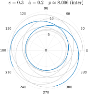
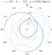
Figure 15: Geodesic equatorial orbits for two different ($e$, ${\hat{a}}$, $p$) configurations. We have highlighted one radial orbit for each configuration. The corresponding waveforms are shown in Fig. 16 and Fig. 17.

Since in the main discussion we have analyzed in detail only the quadrupolar waveform and in Fig. 10 we have shown only the ${\ell}=m=2$ and ${\ell}=m=4$ modes, in this appendix we report almost all the modes up to ${\ell}=8$ for two eccentric cases. The two geodesic dynamics considered are shown in Fig. 15, while the waveform multipoles are reported in Fig. 16 and Fig. 17.

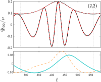
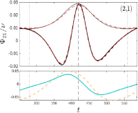
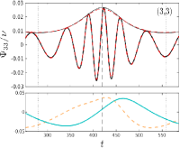
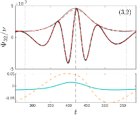
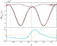
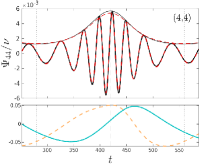
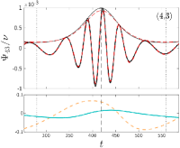
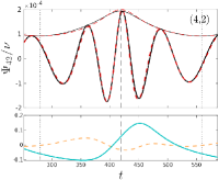
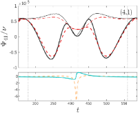
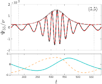
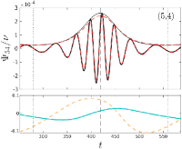
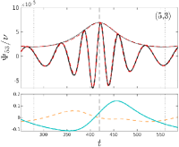
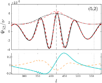
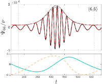
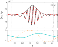
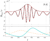
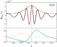
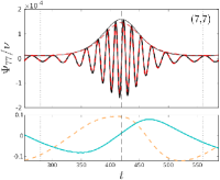
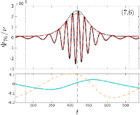
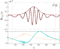
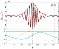
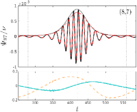
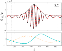
Figure 16: Numerical (black) and EOB (dashed-red) waveform multipoles for the intermediate simulation with $e=0.3$ and ${\hat{a}}=0.2$, whose orbits are shown in Fig. 15. For each multipole, we report the relative amplitude difference (dashed orange) and the phase difference (light blue). The vertical lines mark the periastron and the apastron.

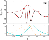
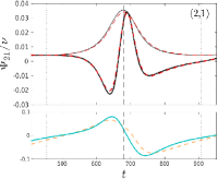
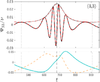
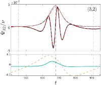
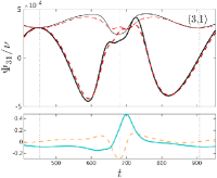
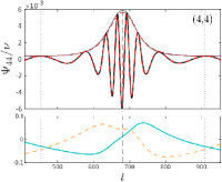
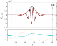
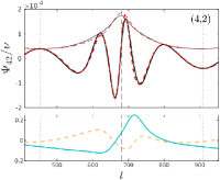
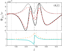
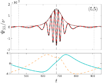
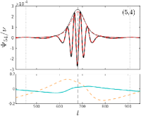
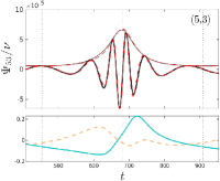
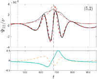
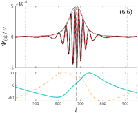
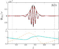
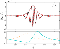
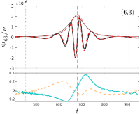
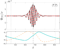
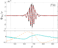
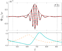
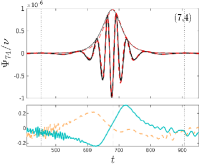
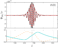
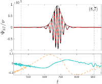
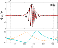
Figure 17: Numerical (black) and EOB (dashed-red) waveform multipoles for the intermediate simulation with $e=0.5$ and ${\hat{a}}=-0.2$, whose orbits are shown in Fig. 15. For each multipole, we report the relative amplitude difference (dashed orange) and the phase difference (light blue). The vertical lines mark the periastron and the apastron.

Appendix D Analytical/numerical fluxes disagreement

In this Appendix we list all the numerical simulations analyzed in this work and we compare the corresponding averaged fluxes. In Table 5, Table 6 and Table 7 we report all the numerical energy and angular momentum averaged fluxes and the corresponding analytical fluxes ${\langle{\dot{F}_{\rm NP}}\rangle}$ computed using the standard radiation reaction ${\hat{{\cal F}}_{\varphi}^{\rm NP}}$ of Eq. (25). The numerical energy fluxes are computed without considering the modes with $m=0$ in order to be coherent with the analytical results. We also recall that these relative differences are plotted against the spin ${\hat{a}}$ in Fig. 7 and against $r_{-}-r_{\rm LR}$ in Fig. 8.

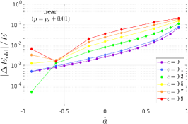
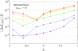
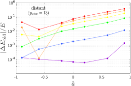
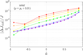
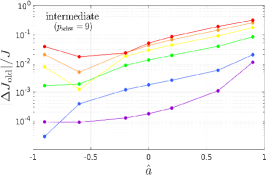
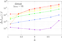
Figure 18: Relative differences between numerical and analytical averaged fluxes plotted against the spin (absolute value, logarithmic scale). Here we consider ${\dot{F}_{\rm old}}$, the fluxes computed with the angular radiation reaction of Eq. (22). The analogous plots for ${\dot{F}_{\rm NP}}$ are shown in Fig. 7.

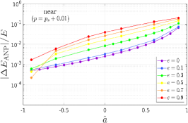
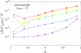
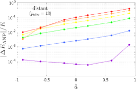
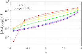
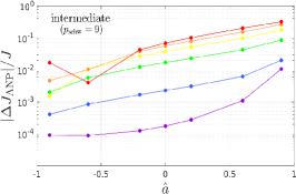
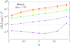
Figure 19: Analogous of Fig. 18 for the ${\dot{F}_{\rm ANP}}$, the fluxes obtained with the angular radiation reaction of Eq. (26).

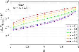
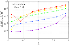
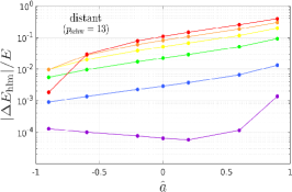
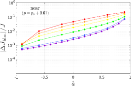
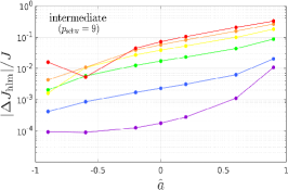
Figure 20: Analogous of Fig. 18 for the fluxes computed using the EOB waveform and Eq. (13).

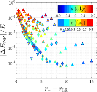
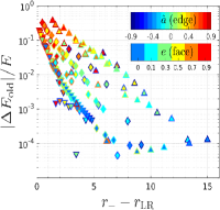
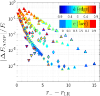
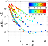
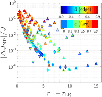
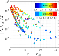
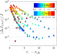
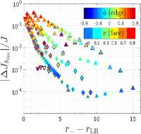
Figure 21: Absolute values of the relative difference between numerical and analytical fluxes averaged along a radial orbits for all the analytical prescriptions studied in this work (see Sec. III.2 for more details). The face color of the markers indicates the eccentricity, while the edge color indicates the spin. The shape of the markers is related to the rule used for the semilatus rectum: the reverse triangle indicates the near simulations ($p=p_{s}+0.01$), the diamond is for the intermediate simulations ( $p=9\;p_{s}(e,{\hat{a}})/p_{s}(e,0)$ ) and the triangle pointing upward indicates the distant simulations ($p=13\;p_{s}(e,{\hat{a}})/p_{s}(e,0)$).

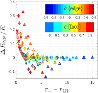
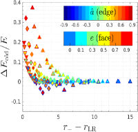
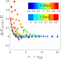
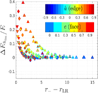
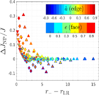
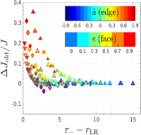
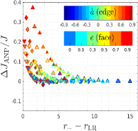
Figure 22: Same relative differences $\Delta F_{\rm analyt}/F=({\langle{\dot{F}_{\rm teuk}}\rangle}-{\langle\dot{F}_{\rm analyt}\rangle})/{\langle{\dot{F}_{\rm teuk}}\rangle}$ of Fig. 21, but without absolute value and logscale.

We also report the analytical/disagreement for the other analytical prescriptions: ${\langle{\dot{F}_{\rm old}}\rangle}$, ${\langle{\dot{F}_{\rm ANP}}\rangle}$, and ${\langle{\dot{F}_{h_{{\ell m}}}}\rangle}$ (see Sec. III.2 for more details). We plot them against the spin ${\hat{a}}$ in Fig. 18, Fig. 19 and Fig. 20 and against $r_{-}-r_{\rm LR}$ in Fig. 21 and Fig. 22. The numerical values of the relative differences between numerical and analytical averaged fluxes obtained adopting the different analytical prescriptions can be found in in Table 8 and Table 9.

Table 5: List of simulations used in our tests with corresponding numerical/analytical averaged fluxes and relative differences. For each eccentricity, there are three blocks of simulations, one for each class of semilatera recta: near, intermediate and distant. The semilatus recta are truncated to the third decimal, see Sec. II.5.

$e$	${\hat{a}}$	$p$	$p_{s}$	${\langle{\dot{E}_{\rm teuk}}\rangle}$	${\langle{\dot{E}_{\rm NP}}\rangle}$	$\Delta E_{\rm NP}/E$	${\langle{\dot{J}_{\rm teuk}}\rangle}$	${\langle{\dot{J}_{\rm NP}}\rangle}$	$\Delta J_{\rm NP}/J$
$0.0$	$-0.9$	$8.727$	$8.717$	$1.732\cdot 10^{-4}$	$1.731\cdot 10^{-4}$	$4.9\cdot 10^{-4}$	$4.309\cdot 10^{-3}$	$4.307\cdot 10^{-3}$	$4.9\cdot 10^{-4}$
$0.0$	$-0.8$	$8.442$	$8.432$	$2.017\cdot 10^{-4}$	$2.016\cdot 10^{-4}$	$5.7\cdot 10^{-4}$	$4.786\cdot 10^{-3}$	$4.783\cdot 10^{-3}$	$5.7\cdot 10^{-4}$
$0.0$	$-0.7$	$8.153$	$8.143$	$2.365\cdot 10^{-4}$	$2.364\cdot 10^{-4}$	$6.7\cdot 10^{-4}$	$5.341\cdot 10^{-3}$	$5.337\cdot 10^{-3}$	$6.7\cdot 10^{-4}$
$0.0$	$-0.6$	$7.861$	$7.851$	$2.794\cdot 10^{-4}$	$2.792\cdot 10^{-4}$	$7.9\cdot 10^{-4}$	$5.991\cdot 10^{-3}$	$5.986\cdot 10^{-3}$	$7.9\cdot 10^{-4}$
$0.0$	$-0.5$	$7.565$	$7.555$	$3.326\cdot 10^{-4}$	$3.323\cdot 10^{-4}$	$9.4\cdot 10^{-4}$	$6.754\cdot 10^{-3}$	$6.748\cdot 10^{-3}$	$9.4\cdot 10^{-4}$
$0.0$	$-0.4$	$7.264$	$7.254$	$3.995\cdot 10^{-4}$	$3.990\cdot 10^{-4}$	$1.1\cdot 10^{-3}$	$7.661\cdot 10^{-3}$	$7.653\cdot 10^{-3}$	$1.1\cdot 10^{-3}$
$0.0$	$-0.3$	$6.959$	$6.949$	$4.843\cdot 10^{-4}$	$4.836\cdot 10^{-4}$	$1.4\cdot 10^{-3}$	$8.745\cdot 10^{-3}$	$8.734\cdot 10^{-3}$	$1.4\cdot 10^{-3}$
$0.0$	$-0.2$	$6.649$	$6.639$	$5.938\cdot 10^{-4}$	$5.928\cdot 10^{-4}$	$1.7\cdot 10^{-3}$	$1.006\cdot 10^{-2}$	$1.004\cdot 10^{-2}$	$1.7\cdot 10^{-3}$
$0.0$	$-0.1$	$6.333$	$6.323$	$7.374\cdot 10^{-4}$	$7.359\cdot 10^{-4}$	$2.0\cdot 10^{-3}$	$1.168\cdot 10^{-2}$	$1.165\cdot 10^{-2}$	$2.0\cdot 10^{-3}$
$0.0$	$0.0$	$6.010$	$6.000$	$9.287\cdot 10^{-4}$	$9.264\cdot 10^{-4}$	$2.5\cdot 10^{-3}$	$1.368\cdot 10^{-2}$	$1.365\cdot 10^{-2}$	$2.5\cdot 10^{-3}$
$0.0$	$0.1$	$5.679$	$5.669$	$1.189\cdot 10^{-3}$	$1.185\cdot 10^{-3}$	$3.2\cdot 10^{-3}$	$1.621\cdot 10^{-2}$	$1.616\cdot 10^{-2}$	$3.2\cdot 10^{-3}$
$0.0$	$0.2$	$5.339$	$5.329$	$1.553\cdot 10^{-3}$	$1.547\cdot 10^{-3}$	$4.0\cdot 10^{-3}$	$1.947\cdot 10^{-2}$	$1.939\cdot 10^{-2}$	$4.0\cdot 10^{-3}$
$0.0$	$0.3$	$4.989$	$4.979$	$2.075\cdot 10^{-3}$	$2.064\cdot 10^{-3}$	$5.2\cdot 10^{-3}$	$2.375\cdot 10^{-2}$	$2.362\cdot 10^{-2}$	$5.2\cdot 10^{-3}$
$0.0$	$0.4$	$4.624$	$4.614$	$2.857\cdot 10^{-3}$	$2.837\cdot 10^{-3}$	$6.9\cdot 10^{-3}$	$2.955\cdot 10^{-2}$	$2.935\cdot 10^{-2}$	$6.9\cdot 10^{-3}$
$0.0$	$0.5$	$4.243$	$4.233$	$4.072\cdot 10^{-3}$	$4.034\cdot 10^{-3}$	$9.4\cdot 10^{-3}$	$3.763\cdot 10^{-2}$	$3.728\cdot 10^{-2}$	$9.4\cdot 10^{-3}$
$0.0$	$0.6$	$3.839$	$3.829$	$6.089\cdot 10^{-3}$	$6.008\cdot 10^{-3}$	$1.3\cdot 10^{-2}$	$4.945\cdot 10^{-2}$	$4.880\cdot 10^{-2}$	$1.3\cdot 10^{-2}$
$0.0$	$0.7$	$3.403$	$3.393$	$9.715\cdot 10^{-3}$	$9.520\cdot 10^{-3}$	$2.0\cdot 10^{-2}$	$6.779\cdot 10^{-2}$	$6.643\cdot 10^{-2}$	$2.0\cdot 10^{-2}$
$0.0$	$0.8$	$2.917$	$2.907$	$1.709\cdot 10^{-2}$	$1.652\cdot 10^{-2}$	$3.3\cdot 10^{-2}$	$9.882\cdot 10^{-2}$	$9.551\cdot 10^{-2}$	$3.3\cdot 10^{-2}$
$0.0$	$0.9$	$2.331$	$2.321$	$3.552\cdot 10^{-2}$	$3.312\cdot 10^{-2}$	$6.7\cdot 10^{-2}$	$1.583\cdot 10^{-1}$	$1.477\cdot 10^{-1}$	$6.7\cdot 10^{-2}$
$0.0$	$-0.9$	$13.076$	$8.717$	$1.837\cdot 10^{-5}$	$1.837\cdot 10^{-5}$	$9.1\cdot 10^{-5}$	$8.520\cdot 10^{-4}$	$8.519\cdot 10^{-4}$	$9.2\cdot 10^{-5}$
$0.0$	$-0.6$	$11.776$	$7.851$	$3.015\cdot 10^{-5}$	$3.015\cdot 10^{-5}$	$8.8\cdot 10^{-5}$	$1.200\cdot 10^{-3}$	$1.200\cdot 10^{-3}$	$8.9\cdot 10^{-5}$
$0.0$	$-0.2$	$9.959$	$6.639$	$6.618\cdot 10^{-5}$	$6.617\cdot 10^{-5}$	$1.3\cdot 10^{-4}$	$2.066\cdot 10^{-3}$	$2.066\cdot 10^{-3}$	$1.3\cdot 10^{-4}$
$0.0$	$0.0$	$9.000$	$6.000$	$1.059\cdot 10^{-4}$	$1.059\cdot 10^{-4}$	$1.8\cdot 10^{-4}$	$2.859\cdot 10^{-3}$	$2.859\cdot 10^{-3}$	$1.8\cdot 10^{-4}$
$0.0$	$0.2$	$7.994$	$5.329$	$1.827\cdot 10^{-4}$	$1.827\cdot 10^{-4}$	$2.8\cdot 10^{-4}$	$4.167\cdot 10^{-3}$	$4.166\cdot 10^{-3}$	$2.8\cdot 10^{-4}$
$0.0$	$0.6$	$5.744$	$3.829$	$8.083\cdot 10^{-4}$	$8.074\cdot 10^{-4}$	$1.1\cdot 10^{-3}$	$1.161\cdot 10^{-2}$	$1.160\cdot 10^{-2}$	$1.1\cdot 10^{-3}$
$0.0$	$0.9$	$3.481$	$2.321$	$6.623\cdot 10^{-3}$	$6.552\cdot 10^{-3}$	$1.1\cdot 10^{-2}$	$4.898\cdot 10^{-2}$	$4.846\cdot 10^{-2}$	$1.1\cdot 10^{-2}$
$0.0$	$-0.9$	$18.888$	$8.717$	$2.702\cdot 10^{-6}$	$2.702\cdot 10^{-6}$	$1.3\cdot 10^{-4}$	$2.194\cdot 10^{-4}$	$2.194\cdot 10^{-4}$	$1.4\cdot 10^{-4}$
$0.0$	$-0.6$	$17.010$	$7.851$	$4.477\cdot 10^{-6}$	$4.476\cdot 10^{-6}$	$9.9\cdot 10^{-5}$	$3.114\cdot 10^{-4}$	$3.114\cdot 10^{-4}$	$1.1\cdot 10^{-4}$
$0.0$	$-0.2$	$14.385$	$6.639$	$1.000\cdot 10^{-5}$	$1.000\cdot 10^{-5}$	$7.6\cdot 10^{-5}$	$5.438\cdot 10^{-4}$	$5.438\cdot 10^{-4}$	$7.6\cdot 10^{-5}$
$0.0$	$0.0$	$13.000$	$6.000$	$1.621\cdot 10^{-5}$	$1.621\cdot 10^{-5}$	$6.5\cdot 10^{-5}$	$7.598\cdot 10^{-4}$	$7.597\cdot 10^{-4}$	$6.2\cdot 10^{-5}$
$0.0$	$0.2$	$11.547$	$5.329$	$2.843\cdot 10^{-5}$	$2.843\cdot 10^{-5}$	$5.8\cdot 10^{-5}$	$1.121\cdot 10^{-3}$	$1.121\cdot 10^{-3}$	$5.8\cdot 10^{-5}$
$0.0$	$0.6$	$8.296$	$3.829$	$1.336\cdot 10^{-4}$	$1.335\cdot 10^{-4}$	$1.1\cdot 10^{-4}$	$3.272\cdot 10^{-3}$	$3.271\cdot 10^{-3}$	$1.1\cdot 10^{-4}$
$0.0$	$0.9$	$5.029$	$2.321$	$1.280\cdot 10^{-3}$	$1.278\cdot 10^{-3}$	$1.4\cdot 10^{-3}$	$1.558\cdot 10^{-2}$	$1.556\cdot 10^{-2}$	$1.4\cdot 10^{-3}$
$0.1$	$-0.9$	$9.014$	$9.004$	$1.870\cdot 10^{-4}$	$1.869\cdot 10^{-4}$	$3.8\cdot 10^{-4}$	$4.505\cdot 10^{-3}$	$4.503\cdot 10^{-3}$	$4.3\cdot 10^{-4}$
$0.1$	$-0.6$	$8.119$	$8.109$	$3.002\cdot 10^{-4}$	$3.000\cdot 10^{-4}$	$7.8\cdot 10^{-4}$	$6.241\cdot 10^{-3}$	$6.236\cdot 10^{-3}$	$8.2\cdot 10^{-4}$
$0.1$	$-0.2$	$6.869$	$6.859$	$6.329\cdot 10^{-4}$	$6.317\cdot 10^{-4}$	$1.9\cdot 10^{-3}$	$1.042\cdot 10^{-2}$	$1.040\cdot 10^{-2}$	$1.9\cdot 10^{-3}$
$0.1$	$0.0$	$6.210$	$6.200$	$9.845\cdot 10^{-4}$	$9.814\cdot 10^{-4}$	$3.1\cdot 10^{-3}$	$1.412\cdot 10^{-2}$	$1.408\cdot 10^{-2}$	$3.0\cdot 10^{-3}$
$0.1$	$0.2$	$5.518$	$5.508$	$1.636\cdot 10^{-3}$	$1.628\cdot 10^{-3}$	$5.0\cdot 10^{-3}$	$2.001\cdot 10^{-2}$	$1.991\cdot 10^{-2}$	$4.9\cdot 10^{-3}$
$0.1$	$0.6$	$3.970$	$3.960$	$6.300\cdot 10^{-3}$	$6.200\cdot 10^{-3}$	$1.6\cdot 10^{-2}$	$5.022\cdot 10^{-2}$	$4.945\cdot 10^{-2}$	$1.6\cdot 10^{-2}$
$0.1$	$0.9$	$2.415$	$2.405$	$3.566\cdot 10^{-2}$	$3.308\cdot 10^{-2}$	$7.2\cdot 10^{-2}$	$1.578\cdot 10^{-1}$	$1.466\cdot 10^{-1}$	$7.1\cdot 10^{-2}$
$0.1$	$-0.9$	$13.070$	$9.004$	$1.897\cdot 10^{-5}$	$1.901\cdot 10^{-5}$	$-2.1\cdot 10^{-3}$	$8.583\cdot 10^{-4}$	$8.593\cdot 10^{-4}$	$-1.2\cdot 10^{-3}$
$0.1$	$-0.6$	$11.772$	$8.109$	$3.112\cdot 10^{-5}$	$3.117\cdot 10^{-5}$	$-1.7\cdot 10^{-3}$	$1.209\cdot 10^{-3}$	$1.210\cdot 10^{-3}$	$-8.1\cdot 10^{-4}$
$0.1$	$-0.2$	$9.957$	$6.859$	$6.825\cdot 10^{-5}$	$6.830\cdot 10^{-5}$	$-8.3\cdot 10^{-4}$	$2.081\cdot 10^{-3}$	$2.081\cdot 10^{-3}$	$-6.0\cdot 10^{-5}$
$0.1$	$0.0$	$9.000$	$6.200$	$1.091\cdot 10^{-4}$	$1.092\cdot 10^{-4}$	$-1.8\cdot 10^{-4}$	$2.878\cdot 10^{-3}$	$2.877\cdot 10^{-3}$	$4.9\cdot 10^{-4}$
$0.1$	$0.2$	$7.996$	$5.508$	$1.882\cdot 10^{-4}$	$1.880\cdot 10^{-4}$	$7.2\cdot 10^{-4}$	$4.194\cdot 10^{-3}$	$4.188\cdot 10^{-3}$	$1.2\cdot 10^{-3}$
$0.1$	$0.6$	$5.749$	$3.960$	$8.299\cdot 10^{-4}$	$8.262\cdot 10^{-4}$	$4.5\cdot 10^{-3}$	$1.167\cdot 10^{-2}$	$1.162\cdot 10^{-2}$	$4.4\cdot 10^{-3}$
$0.1$	$0.9$	$3.491$	$2.405$	$6.735\cdot 10^{-3}$	$6.596\cdot 10^{-3}$	$2.1\cdot 10^{-2}$	$4.903\cdot 10^{-2}$	$4.811\cdot 10^{-2}$	$1.9\cdot 10^{-2}$
$0.1$	$-0.9$	$18.879$	$9.004$	$2.768\cdot 10^{-6}$	$2.773\cdot 10^{-6}$	$-1.8\cdot 10^{-3}$	$2.196\cdot 10^{-4}$	$2.198\cdot 10^{-4}$	$-8.6\cdot 10^{-4}$
$0.1$	$-0.6$	$17.004$	$8.109$	$4.584\cdot 10^{-6}$	$4.590\cdot 10^{-6}$	$-1.5\cdot 10^{-3}$	$3.117\cdot 10^{-4}$	$3.118\cdot 10^{-4}$	$-6.0\cdot 10^{-4}$
$0.1$	$-0.2$	$14.382$	$6.859$	$1.023\cdot 10^{-5}$	$1.024\cdot 10^{-5}$	$-9.1\cdot 10^{-4}$	$5.440\cdot 10^{-4}$	$5.441\cdot 10^{-4}$	$-6.7\cdot 10^{-5}$
$0.1$	$0.0$	$13.000$	$6.200$	$1.657\cdot 10^{-5}$	$1.658\cdot 10^{-5}$	$-4.7\cdot 10^{-4}$	$7.598\cdot 10^{-4}$	$7.596\cdot 10^{-4}$	$3.2\cdot 10^{-4}$
$0.1$	$0.2$	$11.549$	$5.508$	$2.904\cdot 10^{-5}$	$2.904\cdot 10^{-5}$	$1.2\cdot 10^{-4}$	$1.121\cdot 10^{-3}$	$1.120\cdot 10^{-3}$	$8.4\cdot 10^{-4}$
$0.1$	$0.6$	$8.304$	$3.960$	$1.360\cdot 10^{-4}$	$1.357\cdot 10^{-4}$	$2.4\cdot 10^{-3}$	$3.266\cdot 10^{-3}$	$3.257\cdot 10^{-3}$	$2.7\cdot 10^{-3}$
$0.1$	$0.9$	$5.043$	$2.405$	$1.293\cdot 10^{-3}$	$1.281\cdot 10^{-3}$	$8.8\cdot 10^{-3}$	$1.549\cdot 10^{-2}$	$1.537\cdot 10^{-2}$	$7.9\cdot 10^{-3}$

Table 6: Same scheme as Table 5.

$e$	${\hat{a}}$	$p$	$p_{s}$	${\langle{\dot{E}_{\rm teuk}}\rangle}$	${\langle{\dot{E}_{\rm NP}}\rangle}$	$\Delta E_{\rm NP}/E$	${\langle{\dot{J}_{\rm teuk}}\rangle}$	${\langle{\dot{J}_{\rm NP}}\rangle}$	$\Delta J_{\rm NP}/J$
$0.3$	$-0.9$	$9.564$	$9.554$	$2.546\cdot 10^{-4}$	$2.550\cdot 10^{-4}$	$-1.4\cdot 10^{-3}$	$5.324\cdot 10^{-3}$	$5.330\cdot 10^{-3}$	$-1.1\cdot 10^{-3}$
$0.3$	$-0.6$	$8.622$	$8.612$	$4.055\cdot 10^{-4}$	$4.056\cdot 10^{-4}$	$-2.0\cdot 10^{-4}$	$7.339\cdot 10^{-3}$	$7.337\cdot 10^{-3}$	$1.9\cdot 10^{-4}$
$0.3$	$-0.2$	$7.305$	$7.295$	$8.426\cdot 10^{-4}$	$8.400\cdot 10^{-4}$	$3.0\cdot 10^{-3}$	$1.215\cdot 10^{-2}$	$1.211\cdot 10^{-2}$	$3.3\cdot 10^{-3}$
$0.3$	$0.0$	$6.610$	$6.600$	$1.298\cdot 10^{-3}$	$1.291\cdot 10^{-3}$	$5.9\cdot 10^{-3}$	$1.637\cdot 10^{-2}$	$1.627\cdot 10^{-2}$	$6.2\cdot 10^{-3}$
$0.3$	$0.1$	$6.250$	$6.240$	$1.648\cdot 10^{-3}$	$1.635\cdot 10^{-3}$	$7.9\cdot 10^{-3}$	$1.929\cdot 10^{-2}$	$1.913\cdot 10^{-2}$	$8.1\cdot 10^{-3}$
$0.3$	$0.2$	$5.881$	$5.871$	$2.131\cdot 10^{-3}$	$2.109\cdot 10^{-3}$	$1.1\cdot 10^{-2}$	$2.302\cdot 10^{-2}$	$2.278\cdot 10^{-2}$	$1.1\cdot 10^{-2}$
$0.3$	$0.3$	$5.500$	$5.490$	$2.817\cdot 10^{-3}$	$2.777\cdot 10^{-3}$	$1.4\cdot 10^{-2}$	$2.789\cdot 10^{-2}$	$2.750\cdot 10^{-2}$	$1.4\cdot 10^{-2}$
$0.3$	$0.4$	$5.104$	$5.094$	$3.824\cdot 10^{-3}$	$3.754\cdot 10^{-3}$	$1.8\cdot 10^{-2}$	$3.440\cdot 10^{-2}$	$3.378\cdot 10^{-2}$	$1.8\cdot 10^{-2}$
$0.3$	$0.5$	$4.689$	$4.679$	$5.366\cdot 10^{-3}$	$5.235\cdot 10^{-3}$	$2.4\cdot 10^{-2}$	$4.339\cdot 10^{-2}$	$4.236\cdot 10^{-2}$	$2.4\cdot 10^{-2}$
$0.3$	$0.6$	$4.250$	$4.240$	$7.862\cdot 10^{-3}$	$7.602\cdot 10^{-3}$	$3.3\cdot 10^{-2}$	$5.630\cdot 10^{-2}$	$5.451\cdot 10^{-2}$	$3.2\cdot 10^{-2}$
$0.3$	$0.7$	$3.777$	$3.767$	$1.221\cdot 10^{-2}$	$1.165\cdot 10^{-2}$	$4.6\cdot 10^{-2}$	$7.590\cdot 10^{-2}$	$7.256\cdot 10^{-2}$	$4.4\cdot 10^{-2}$
$0.3$	$0.8$	$3.249$	$3.239$	$2.065\cdot 10^{-2}$	$1.926\cdot 10^{-2}$	$6.7\cdot 10^{-2}$	$1.078\cdot 10^{-1}$	$1.009\cdot 10^{-1}$	$6.4\cdot 10^{-2}$
$0.3$	$0.9$	$2.615$	$2.605$	$4.030\cdot 10^{-2}$	$3.602\cdot 10^{-2}$	$1.1\cdot 10^{-1}$	$1.662\cdot 10^{-1}$	$1.495\cdot 10^{-1}$	$1.0\cdot 10^{-1}$
$0.3$	$-0.9$	$13.028$	$9.554$	$2.350\cdot 10^{-5}$	$2.392\cdot 10^{-5}$	$-1.8\cdot 10^{-2}$	$8.995\cdot 10^{-4}$	$9.095\cdot 10^{-4}$	$-1.1\cdot 10^{-2}$
$0.3$	$-0.6$	$11.743$	$8.612$	$3.843\cdot 10^{-5}$	$3.898\cdot 10^{-5}$	$-1.4\cdot 10^{-2}$	$1.265\cdot 10^{-3}$	$1.275\cdot 10^{-3}$	$-7.9\cdot 10^{-3}$
$0.3$	$-0.2$	$9.947$	$7.295$	$8.381\cdot 10^{-5}$	$8.443\cdot 10^{-5}$	$-7.4\cdot 10^{-3}$	$2.174\cdot 10^{-3}$	$2.178\cdot 10^{-3}$	$-1.7\cdot 10^{-3}$
$0.3$	$0.0$	$9.000$	$6.600$	$1.335\cdot 10^{-4}$	$1.338\cdot 10^{-4}$	$-2.5\cdot 10^{-3}$	$3.004\cdot 10^{-3}$	$2.996\cdot 10^{-3}$	$2.6\cdot 10^{-3}$
$0.3$	$0.2$	$8.006$	$5.871$	$2.289\cdot 10^{-4}$	$2.280\cdot 10^{-4}$	$4.1\cdot 10^{-3}$	$4.369\cdot 10^{-3}$	$4.333\cdot 10^{-3}$	$8.2\cdot 10^{-3}$
$0.3$	$0.6$	$5.782$	$4.240$	$9.889\cdot 10^{-4}$	$9.612\cdot 10^{-4}$	$2.8\cdot 10^{-2}$	$1.207\cdot 10^{-2}$	$1.173\cdot 10^{-2}$	$2.8\cdot 10^{-2}$
$0.3$	$0.9$	$3.553$	$2.605$	$7.574\cdot 10^{-3}$	$6.922\cdot 10^{-3}$	$8.6\cdot 10^{-2}$	$4.941\cdot 10^{-2}$	$4.575\cdot 10^{-2}$	$7.4\cdot 10^{-2}$
$0.3$	$-0.9$	$18.818$	$9.554$	$3.231\cdot 10^{-6}$	$3.284\cdot 10^{-6}$	$-1.6\cdot 10^{-2}$	$2.191\cdot 10^{-4}$	$2.211\cdot 10^{-4}$	$-9.0\cdot 10^{-3}$
$0.3$	$-0.6$	$16.962$	$8.612$	$5.333\cdot 10^{-6}$	$5.405\cdot 10^{-6}$	$-1.3\cdot 10^{-2}$	$3.105\cdot 10^{-4}$	$3.124\cdot 10^{-4}$	$-6.3\cdot 10^{-3}$
$0.3$	$-0.2$	$14.368$	$7.295$	$1.184\cdot 10^{-5}$	$1.193\cdot 10^{-5}$	$-7.8\cdot 10^{-3}$	$5.407\cdot 10^{-4}$	$5.413\cdot 10^{-4}$	$-1.2\cdot 10^{-3}$
$0.3$	$0.0$	$13.000$	$6.600$	$1.910\cdot 10^{-5}$	$1.918\cdot 10^{-5}$	$-3.9\cdot 10^{-3}$	$7.540\cdot 10^{-4}$	$7.522\cdot 10^{-4}$	$2.3\cdot 10^{-3}$
$0.3$	$0.2$	$11.564$	$5.871$	$3.331\cdot 10^{-5}$	$3.327\cdot 10^{-5}$	$1.4\cdot 10^{-3}$	$1.110\cdot 10^{-3}$	$1.102\cdot 10^{-3}$	$7.0\cdot 10^{-3}$
$0.3$	$0.6$	$8.352$	$4.240$	$1.533\cdot 10^{-4}$	$1.503\cdot 10^{-4}$	$2.0\cdot 10^{-2}$	$3.211\cdot 10^{-3}$	$3.137\cdot 10^{-3}$	$2.3\cdot 10^{-2}$
$0.3$	$0.9$	$5.132$	$2.605$	$1.389\cdot 10^{-3}$	$1.305\cdot 10^{-3}$	$6.1\cdot 10^{-2}$	$1.489\cdot 10^{-2}$	$1.407\cdot 10^{-2}$	$5.5\cdot 10^{-2}$
$0.5$	$-0.9$	$10.089$	$10.079$	$3.287\cdot 10^{-4}$	$3.302\cdot 10^{-4}$	$-4.6\cdot 10^{-3}$	$5.933\cdot 10^{-3}$	$5.958\cdot 10^{-3}$	$-4.2\cdot 10^{-3}$
$0.5$	$-0.6$	$9.107$	$9.097$	$5.198\cdot 10^{-4}$	$5.208\cdot 10^{-4}$	$-2.0\cdot 10^{-3}$	$8.149\cdot 10^{-3}$	$8.160\cdot 10^{-3}$	$-1.4\cdot 10^{-3}$
$0.5$	$-0.2$	$7.734$	$7.724$	$1.067\cdot 10^{-3}$	$1.062\cdot 10^{-3}$	$4.7\cdot 10^{-3}$	$1.341\cdot 10^{-2}$	$1.334\cdot 10^{-2}$	$5.5\cdot 10^{-3}$
$0.5$	$0.0$	$7.010$	$7.000$	$1.630\cdot 10^{-3}$	$1.613\cdot 10^{-3}$	$1.1\cdot 10^{-2}$	$1.799\cdot 10^{-2}$	$1.779\cdot 10^{-2}$	$1.1\cdot 10^{-2}$
$0.5$	$0.2$	$6.250$	$6.240$	$2.647\cdot 10^{-3}$	$2.595\cdot 10^{-3}$	$2.0\cdot 10^{-2}$	$2.517\cdot 10^{-2}$	$2.466\cdot 10^{-2}$	$2.0\cdot 10^{-2}$
$0.5$	$0.6$	$4.548$	$4.538$	$9.403\cdot 10^{-3}$	$8.859\cdot 10^{-3}$	$5.8\cdot 10^{-2}$	$6.039\cdot 10^{-2}$	$5.693\cdot 10^{-2}$	$5.7\cdot 10^{-2}$
$0.5$	$0.9$	$2.843$	$2.833$	$4.424\cdot 10^{-2}$	$3.792\cdot 10^{-2}$	$1.4\cdot 10^{-1}$	$1.696\cdot 10^{-1}$	$1.463\cdot 10^{-1}$	$1.4\cdot 10^{-1}$
$0.5$	$-0.9$	$12.959$	$10.079$	$3.078\cdot 10^{-5}$	$3.211\cdot 10^{-5}$	$-4.3\cdot 10^{-2}$	$9.314\cdot 10^{-4}$	$9.592\cdot 10^{-4}$	$-3.0\cdot 10^{-2}$
$0.5$	$-0.6$	$11.697$	$9.097$	$5.009\cdot 10^{-5}$	$5.182\cdot 10^{-5}$	$-3.5\cdot 10^{-2}$	$1.309\cdot 10^{-3}$	$1.337\cdot 10^{-3}$	$-2.1\cdot 10^{-2}$
$0.5$	$-0.2$	$9.931$	$7.724$	$1.082\cdot 10^{-4}$	$1.102\cdot 10^{-4}$	$-1.8\cdot 10^{-2}$	$2.243\cdot 10^{-3}$	$2.256\cdot 10^{-3}$	$-5.9\cdot 10^{-3}$
$0.5$	$0.0$	$9.000$	$7.000$	$1.713\cdot 10^{-4}$	$1.723\cdot 10^{-4}$	$-5.8\cdot 10^{-3}$	$3.093\cdot 10^{-3}$	$3.078\cdot 10^{-3}$	$4.9\cdot 10^{-3}$
$0.5$	$0.2$	$8.022$	$6.240$	$2.914\cdot 10^{-4}$	$2.885\cdot 10^{-4}$	$1.0\cdot 10^{-2}$	$4.488\cdot 10^{-3}$	$4.403\cdot 10^{-3}$	$1.9\cdot 10^{-2}$
$0.5$	$0.6$	$5.834$	$4.538$	$1.222\cdot 10^{-3}$	$1.143\cdot 10^{-3}$	$6.4\cdot 10^{-2}$	$1.228\cdot 10^{-2}$	$1.147\cdot 10^{-2}$	$6.6\cdot 10^{-2}$
$0.5$	$0.9$	$3.643$	$2.833$	$8.674\cdot 10^{-3}$	$7.191\cdot 10^{-3}$	$1.7\cdot 10^{-1}$	$4.867\cdot 10^{-2}$	$4.117\cdot 10^{-2}$	$1.5\cdot 10^{-1}$
$0.5$	$-0.9$	$18.718$	$10.079$	$3.808\cdot 10^{-6}$	$3.973\cdot 10^{-6}$	$-4.3\cdot 10^{-2}$	$2.062\cdot 10^{-4}$	$2.115\cdot 10^{-4}$	$-2.6\cdot 10^{-2}$
$0.5$	$-0.6$	$16.895$	$9.097$	$6.255\cdot 10^{-6}$	$6.473\cdot 10^{-6}$	$-3.5\cdot 10^{-2}$	$2.915\cdot 10^{-4}$	$2.968\cdot 10^{-4}$	$-1.8\cdot 10^{-2}$
$0.5$	$-0.2$	$14.345$	$7.724$	$1.377\cdot 10^{-5}$	$1.403\cdot 10^{-5}$	$-1.9\cdot 10^{-2}$	$5.058\cdot 10^{-4}$	$5.077\cdot 10^{-4}$	$-3.7\cdot 10^{-3}$
$0.5$	$0.0$	$13.000$	$7.000$	$2.208\cdot 10^{-5}$	$2.226\cdot 10^{-5}$	$-8.1\cdot 10^{-3}$	$7.038\cdot 10^{-4}$	$6.995\cdot 10^{-4}$	$6.0\cdot 10^{-3}$
$0.5$	$0.2$	$11.588$	$6.240$	$3.822\cdot 10^{-5}$	$3.799\cdot 10^{-5}$	$6.1\cdot 10^{-3}$	$1.033\cdot 10^{-3}$	$1.014\cdot 10^{-3}$	$1.9\cdot 10^{-2}$
$0.5$	$0.6$	$8.427$	$4.538$	$1.715\cdot 10^{-4}$	$1.624\cdot 10^{-4}$	$5.3\cdot 10^{-2}$	$2.960\cdot 10^{-3}$	$2.785\cdot 10^{-3}$	$5.9\cdot 10^{-2}$
$0.5$	$0.9$	$5.262$	$2.833$	$1.467\cdot 10^{-3}$	$1.259\cdot 10^{-3}$	$1.4\cdot 10^{-1}$	$1.343\cdot 10^{-2}$	$1.165\cdot 10^{-2}$	$1.3\cdot 10^{-1}$

Table 7: Same scheme as Table 5

$e$	${\hat{a}}$	$p$	$p_{s}$	${\langle{\dot{E}_{\rm teuk}}\rangle}$	${\langle{\dot{E}_{\rm NP}}\rangle}$	$\Delta E_{\rm NP}/E$	${\langle{\dot{J}_{\rm teuk}}\rangle}$	${\langle{\dot{J}_{\rm NP}}\rangle}$	$\Delta J_{\rm NP}/J$
$0.7$	$-0.9$	$10.595$	$10.585$	$3.364\cdot 10^{-4}$	$3.394\cdot 10^{-4}$	$-8.9\cdot 10^{-3}$	$5.335\cdot 10^{-3}$	$5.381\cdot 10^{-3}$	$-8.8\cdot 10^{-3}$
$0.7$	$-0.6$	$9.580$	$9.570$	$5.294\cdot 10^{-4}$	$5.316\cdot 10^{-4}$	$-4.2\cdot 10^{-3}$	$7.320\cdot 10^{-3}$	$7.346\cdot 10^{-3}$	$-3.6\cdot 10^{-3}$
$0.7$	$-0.2$	$8.160$	$8.150$	$1.077\cdot 10^{-3}$	$1.070\cdot 10^{-3}$	$7.4\cdot 10^{-3}$	$1.203\cdot 10^{-2}$	$1.193\cdot 10^{-2}$	$8.6\cdot 10^{-3}$
$0.7$	$0.0$	$7.410$	$7.400$	$1.637\cdot 10^{-3}$	$1.609\cdot 10^{-3}$	$1.7\cdot 10^{-2}$	$1.613\cdot 10^{-2}$	$1.583\cdot 10^{-2}$	$1.9\cdot 10^{-2}$
$0.7$	$0.2$	$6.622$	$6.612$	$2.641\cdot 10^{-3}$	$2.558\cdot 10^{-3}$	$3.2\cdot 10^{-2}$	$2.255\cdot 10^{-2}$	$2.181\cdot 10^{-2}$	$3.3\cdot 10^{-2}$
$0.7$	$0.6$	$4.858$	$4.848$	$9.173\cdot 10^{-3}$	$8.375\cdot 10^{-3}$	$8.7\cdot 10^{-2}$	$5.390\cdot 10^{-2}$	$4.916\cdot 10^{-2}$	$8.8\cdot 10^{-2}$
$0.7$	$0.9$	$3.088$	$3.078$	$4.151\cdot 10^{-2}$	$3.437\cdot 10^{-2}$	$1.7\cdot 10^{-1}$	$1.504\cdot 10^{-1}$	$1.249\cdot 10^{-1}$	$1.7\cdot 10^{-1}$
$0.7$	$-0.9$	$12.873$	$10.585$	$3.427\cdot 10^{-5}$	$3.680\cdot 10^{-5}$	$-7.4\cdot 10^{-2}$	$8.231\cdot 10^{-4}$	$8.685\cdot 10^{-4}$	$-5.5\cdot 10^{-2}$
$0.7$	$-0.6$	$11.639$	$9.570$	$5.545\cdot 10^{-5}$	$5.871\cdot 10^{-5}$	$-5.9\cdot 10^{-2}$	$1.155\cdot 10^{-3}$	$1.201\cdot 10^{-3}$	$-4.1\cdot 10^{-2}$
$0.7$	$-0.2$	$9.912$	$8.150$	$1.186\cdot 10^{-4}$	$1.222\cdot 10^{-4}$	$-3.0\cdot 10^{-2}$	$1.974\cdot 10^{-3}$	$2.000\cdot 10^{-3}$	$-1.3\cdot 10^{-2}$
$0.7$	$0.0$	$9.000$	$7.400$	$1.865\cdot 10^{-4}$	$1.882\cdot 10^{-4}$	$-9.2\cdot 10^{-3}$	$2.719\cdot 10^{-3}$	$2.702\cdot 10^{-3}$	$5.9\cdot 10^{-3}$
$0.7$	$0.2$	$8.042$	$6.612$	$3.144\cdot 10^{-4}$	$3.089\cdot 10^{-4}$	$1.8\cdot 10^{-2}$	$3.937\cdot 10^{-3}$	$3.817\cdot 10^{-3}$	$3.0\cdot 10^{-2}$
$0.7$	$0.6$	$5.896$	$4.848$	$1.278\cdot 10^{-3}$	$1.143\cdot 10^{-3}$	$1.1\cdot 10^{-1}$	$1.068\cdot 10^{-2}$	$9.517\cdot 10^{-3}$	$1.1\cdot 10^{-1}$
$0.7$	$0.9$	$3.744$	$3.078$	$8.476\cdot 10^{-3}$	$6.396\cdot 10^{-3}$	$2.5\cdot 10^{-1}$	$4.133\cdot 10^{-2}$	$3.186\cdot 10^{-2}$	$2.3\cdot 10^{-1}$
$0.7$	$-0.9$	$18.595$	$10.585$	$3.648\cdot 10^{-6}$	$3.952\cdot 10^{-6}$	$-8.3\cdot 10^{-2}$	$1.578\cdot 10^{-4}$	$1.660\cdot 10^{-4}$	$-5.2\cdot 10^{-2}$
$0.7$	$-0.6$	$16.812$	$9.570$	$5.957\cdot 10^{-6}$	$6.349\cdot 10^{-6}$	$-6.6\cdot 10^{-2}$	$2.225\cdot 10^{-4}$	$2.307\cdot 10^{-4}$	$-3.7\cdot 10^{-2}$
$0.7$	$-0.2$	$14.317$	$8.150$	$1.298\cdot 10^{-5}$	$1.341\cdot 10^{-5}$	$-3.4\cdot 10^{-2}$	$3.846\cdot 10^{-4}$	$3.879\cdot 10^{-4}$	$-8.5\cdot 10^{-3}$
$0.7$	$0.0$	$13.000$	$7.400$	$2.067\cdot 10^{-5}$	$2.093\cdot 10^{-5}$	$-1.2\cdot 10^{-2}$	$5.338\cdot 10^{-4}$	$5.283\cdot 10^{-4}$	$1.0\cdot 10^{-2}$
$0.7$	$0.2$	$11.616$	$6.612$	$3.548\cdot 10^{-5}$	$3.497\cdot 10^{-5}$	$1.5\cdot 10^{-2}$	$7.815\cdot 10^{-4}$	$7.550\cdot 10^{-4}$	$3.4\cdot 10^{-2}$
$0.7$	$0.6$	$8.517$	$4.848$	$1.550\cdot 10^{-4}$	$1.397\cdot 10^{-4}$	$9.9\cdot 10^{-2}$	$2.219\cdot 10^{-3}$	$1.982\cdot 10^{-3}$	$1.1\cdot 10^{-1}$
$0.7$	$0.9$	$5.408$	$3.078$	$1.257\cdot 10^{-3}$	$9.635\cdot 10^{-4}$	$2.3\cdot 10^{-1}$	$9.906\cdot 10^{-3}$	$7.716\cdot 10^{-3}$	$2.2\cdot 10^{-1}$
$0.9$	$-0.9$	$11.084$	$11.074$	$1.439\cdot 10^{-4}$	$1.460\cdot 10^{-4}$	$-1.5\cdot 10^{-2}$	$2.040\cdot 10^{-3}$	$2.071\cdot 10^{-3}$	$-1.5\cdot 10^{-2}$
$0.9$	$-0.6$	$10.042$	$10.032$	$2.261\cdot 10^{-4}$	$2.277\cdot 10^{-4}$	$-7.2\cdot 10^{-3}$	$2.807\cdot 10^{-3}$	$2.826\cdot 10^{-3}$	$-6.7\cdot 10^{-3}$
$0.9$	$-0.2$	$8.582$	$8.572$	$4.594\cdot 10^{-4}$	$4.544\cdot 10^{-4}$	$1.1\cdot 10^{-2}$	$4.643\cdot 10^{-3}$	$4.585\cdot 10^{-3}$	$1.2\cdot 10^{-2}$
$0.9$	$0.0$	$7.810$	$7.800$	$6.979\cdot 10^{-4}$	$6.799\cdot 10^{-4}$	$2.6\cdot 10^{-2}$	$6.253\cdot 10^{-3}$	$6.080\cdot 10^{-3}$	$2.8\cdot 10^{-2}$
$0.9$	$0.2$	$6.999$	$6.989$	$1.126\cdot 10^{-3}$	$1.073\cdot 10^{-3}$	$4.7\cdot 10^{-2}$	$8.798\cdot 10^{-3}$	$8.368\cdot 10^{-3}$	$4.9\cdot 10^{-2}$
$0.9$	$0.6$	$5.177$	$5.167$	$3.935\cdot 10^{-3}$	$3.467\cdot 10^{-3}$	$1.2\cdot 10^{-1}$	$2.155\cdot 10^{-2}$	$1.894\cdot 10^{-2}$	$1.2\cdot 10^{-1}$
$0.9$	$0.9$	$3.344$	$3.334$	$1.877\cdot 10^{-2}$	$1.516\cdot 10^{-2}$	$1.9\cdot 10^{-1}$	$6.525\cdot 10^{-2}$	$5.270\cdot 10^{-2}$	$1.9\cdot 10^{-1}$
$0.9$	$-0.9$	$12.778$	$11.074$	$1.704\cdot 10^{-5}$	$1.883\cdot 10^{-5}$	$-1.0\cdot 10^{-1}$	$3.320\cdot 10^{-4}$	$3.598\cdot 10^{-4}$	$-8.4\cdot 10^{-2}$
$0.9$	$-0.6$	$11.576$	$10.032$	$2.741\cdot 10^{-5}$	$2.969\cdot 10^{-5}$	$-8.3\cdot 10^{-2}$	$4.654\cdot 10^{-4}$	$4.944\cdot 10^{-4}$	$-6.2\cdot 10^{-2}$
$0.9$	$-0.2$	$9.891$	$8.572$	$5.806\cdot 10^{-5}$	$6.043\cdot 10^{-5}$	$-4.1\cdot 10^{-2}$	$7.946\cdot 10^{-4}$	$8.120\cdot 10^{-4}$	$-2.2\cdot 10^{-2}$
$0.9$	$0.0$	$9.000$	$7.800$	$9.068\cdot 10^{-5}$	$9.169\cdot 10^{-5}$	$-1.1\cdot 10^{-2}$	$1.093\cdot 10^{-3}$	$1.087\cdot 10^{-3}$	$6.1\cdot 10^{-3}$
$0.9$	$0.2$	$8.064$	$6.989$	$1.516\cdot 10^{-4}$	$1.475\cdot 10^{-4}$	$2.7\cdot 10^{-2}$	$1.582\cdot 10^{-3}$	$1.515\cdot 10^{-3}$	$4.2\cdot 10^{-2}$
$0.9$	$0.6$	$5.962$	$5.167$	$5.996\cdot 10^{-4}$	$5.120\cdot 10^{-4}$	$1.5\cdot 10^{-1}$	$4.278\cdot 10^{-3}$	$3.633\cdot 10^{-3}$	$1.5\cdot 10^{-1}$
$0.9$	$0.9$	$3.847$	$3.334$	$3.818\cdot 10^{-3}$	$2.678\cdot 10^{-3}$	$3.0\cdot 10^{-1}$	$1.656\cdot 10^{-2}$	$1.184\cdot 10^{-2}$	$2.8\cdot 10^{-1}$
$0.9$	$-0.9$	$18.457$	$11.074$	$1.474\cdot 10^{-6}$	$1.679\cdot 10^{-6}$	$-1.4\cdot 10^{-1}$	$5.209\cdot 10^{-5}$	$5.684\cdot 10^{-5}$	$-9.1\cdot 10^{-2}$
$0.9$	$-0.6$	$16.720$	$10.032$	$2.391\cdot 10^{-6}$	$2.651\cdot 10^{-6}$	$-1.1\cdot 10^{-1}$	$7.330\cdot 10^{-5}$	$7.803\cdot 10^{-5}$	$-6.5\cdot 10^{-2}$
$0.9$	$-0.2$	$14.287$	$8.572$	$5.151\cdot 10^{-6}$	$5.430\cdot 10^{-6}$	$-5.4\cdot 10^{-2}$	$1.262\cdot 10^{-4}$	$1.284\cdot 10^{-4}$	$-1.7\cdot 10^{-2}$
$0.9$	$0.0$	$13.000$	$7.800$	$8.148\cdot 10^{-6}$	$8.299\cdot 10^{-6}$	$-1.8\cdot 10^{-2}$	$1.747\cdot 10^{-4}$	$1.724\cdot 10^{-4}$	$1.3\cdot 10^{-2}$
$0.9$	$0.2$	$11.648$	$6.989$	$1.387\cdot 10^{-5}$	$1.352\cdot 10^{-5}$	$2.5\cdot 10^{-2}$	$2.550\cdot 10^{-4}$	$2.421\cdot 10^{-4}$	$5.1\cdot 10^{-2}$
$0.9$	$0.6$	$8.612$	$5.167$	$5.904\cdot 10^{-5}$	$5.003\cdot 10^{-5}$	$1.5\cdot 10^{-1}$	$7.194\cdot 10^{-4}$	$6.041\cdot 10^{-4}$	$1.6\cdot 10^{-1}$
$0.9$	$0.9$	$5.557$	$3.334$	$4.602\cdot 10^{-4}$	$3.105\cdot 10^{-4}$	$3.3\cdot 10^{-1}$	$3.196\cdot 10^{-3}$	$2.211\cdot 10^{-3}$	$3.1\cdot 10^{-1}$

Table 8: Analytical/numerical relative differences for the energy and angular momentum fluxes: $\Delta F_{\rm analytic}/F=({\langle{\dot{F}_{\rm teuk}}\rangle}-{\langle\dot{F}_{\rm analytic}\rangle})/{\langle{\dot{F}_{\rm teuk}}\rangle}$. We report both the fluxes computed from the radiation reactions and from the EOB waveform for all the eccentric simulations. Black: $\Delta F/F<1\%$, blue: $1\%\leq\Delta F/F<5\%$, red : $5\%\leq\Delta F/F$.

$e$	${\hat{a}}$	$p$	$p_{s}$	$\Delta E_{\rm NP}/E$	$\Delta E_{\rm old}/E$	$\Delta E_{\rm ANP}/E$	$\Delta E_{h_{\ell m}}/E$	$\Delta J_{\rm NP}/J$	$\Delta J_{\rm old}/J$	$\Delta J_{\rm ANP}/J$	$\Delta J_{h_{\ell m}}/J$
$0.1$	$-0.9$	$9.014$	$9.004$	$3.8\cdot 10^{-4}$	$4.9\cdot 10^{-4}$	$5.5\cdot 10^{-4}$	$6.5\cdot 10^{-4}$	$4.3\cdot 10^{-4}$	$5.2\cdot 10^{-4}$	$5.6\cdot 10^{-4}$	$5.9\cdot 10^{-4}$
$0.1$	$-0.6$	$8.119$	$8.109$	$7.8\cdot 10^{-4}$	$9.0\cdot 10^{-4}$	$9.7\cdot 10^{-4}$	$1.1\cdot 10^{-3}$	$8.2\cdot 10^{-4}$	$9.1\cdot 10^{-4}$	$9.6\cdot 10^{-4}$	$1.0\cdot 10^{-3}$
$0.1$	$-0.2$	$6.869$	$6.859$	$1.9\cdot 10^{-3}$	$2.1\cdot 10^{-3}$	$2.1\cdot 10^{-3}$	$2.2\cdot 10^{-3}$	$1.9\cdot 10^{-3}$	$2.0\cdot 10^{-3}$	$2.1\cdot 10^{-3}$	$2.1\cdot 10^{-3}$
$0.1$	$0.0$	$6.210$	$6.200$	$3.1\cdot 10^{-3}$	$3.2\cdot 10^{-3}$	$3.3\cdot 10^{-3}$	$3.4\cdot 10^{-3}$	$3.0\cdot 10^{-3}$	$3.1\cdot 10^{-3}$	$3.2\cdot 10^{-3}$	$3.2\cdot 10^{-3}$
$0.1$	$0.2$	$5.518$	$5.508$	$5.0\cdot 10^{-3}$	$5.1\cdot 10^{-3}$	$5.2\cdot 10^{-3}$	$5.3\cdot 10^{-3}$	$4.9\cdot 10^{-3}$	$5.0\cdot 10^{-3}$	$5.0\cdot 10^{-3}$	$5.1\cdot 10^{-3}$
$0.1$	$0.6$	$3.970$	$3.960$	$\color[rgb]{0.1,0.1,1.0}1.6\cdot 10^{-2}$	$\color[rgb]{0.1,0.1,1.0}1.6\cdot 10^{-2}$	$\color[rgb]{0.1,0.1,1.0}1.6\cdot 10^{-2}$	$\color[rgb]{0.1,0.1,1.0}1.6\cdot 10^{-2}$	$\color[rgb]{0.1,0.1,1.0}1.6\cdot 10^{-2}$	$\color[rgb]{0.1,0.1,1.0}1.6\cdot 10^{-2}$	$\color[rgb]{0.1,0.1,1.0}1.6\cdot 10^{-2}$	$\color[rgb]{0.1,0.1,1.0}1.6\cdot 10^{-2}$
$0.1$	$0.9$	$2.415$	$2.405$	$\color[rgb]{0.9,0,0.1}7.2\cdot 10^{-2}$	$\color[rgb]{0.9,0,0.1}7.2\cdot 10^{-2}$	$\color[rgb]{0.9,0,0.1}7.2\cdot 10^{-2}$	$\color[rgb]{0.9,0,0.1}7.3\cdot 10^{-2}$	$\color[rgb]{0.9,0,0.1}7.1\cdot 10^{-2}$	$\color[rgb]{0.9,0,0.1}7.1\cdot 10^{-2}$	$\color[rgb]{0.9,0,0.1}7.1\cdot 10^{-2}$	$\color[rgb]{0.9,0,0.1}7.1\cdot 10^{-2}$
$0.1$	$-0.9$	$13.070$	$9.004$	$-2.1\cdot 10^{-3}$	$-4.5\cdot 10^{-4}$	$1.9\cdot 10^{-4}$	$4.4\cdot 10^{-4}$	$-1.2\cdot 10^{-3}$	$-2.9\cdot 10^{-5}$	$4.1\cdot 10^{-4}$	$4.1\cdot 10^{-4}$
$0.1$	$-0.6$	$11.772$	$8.109$	$-1.7\cdot 10^{-3}$	$4.5\cdot 10^{-5}$	$7.1\cdot 10^{-4}$	$1.0\cdot 10^{-3}$	$-8.1\cdot 10^{-4}$	$3.9\cdot 10^{-4}$	$8.5\cdot 10^{-4}$	$8.5\cdot 10^{-4}$
$0.1$	$-0.2$	$9.957$	$6.859$	$-8.3\cdot 10^{-4}$	$1.0\cdot 10^{-3}$	$1.7\cdot 10^{-3}$	$2.1\cdot 10^{-3}$	$-6.0\cdot 10^{-5}$	$1.2\cdot 10^{-3}$	$1.7\cdot 10^{-3}$	$1.7\cdot 10^{-3}$
$0.1$	$0.0$	$9.000$	$6.200$	$-1.8\cdot 10^{-4}$	$1.7\cdot 10^{-3}$	$2.5\cdot 10^{-3}$	$2.9\cdot 10^{-3}$	$4.9\cdot 10^{-4}$	$1.8\cdot 10^{-3}$	$2.3\cdot 10^{-3}$	$2.3\cdot 10^{-3}$
$0.1$	$0.2$	$7.996$	$5.508$	$7.2\cdot 10^{-4}$	$2.6\cdot 10^{-3}$	$3.4\cdot 10^{-3}$	$3.9\cdot 10^{-3}$	$1.2\cdot 10^{-3}$	$2.6\cdot 10^{-3}$	$3.1\cdot 10^{-3}$	$3.1\cdot 10^{-3}$
$0.1$	$0.6$	$5.749$	$3.960$	$4.5\cdot 10^{-3}$	$6.4\cdot 10^{-3}$	$7.3\cdot 10^{-3}$	$7.9\cdot 10^{-3}$	$4.4\cdot 10^{-3}$	$5.7\cdot 10^{-3}$	$6.2\cdot 10^{-3}$	$6.3\cdot 10^{-3}$
$0.1$	$0.9$	$3.491$	$2.405$	$\color[rgb]{0.1,0.1,1.0}2.1\cdot 10^{-2}$	$\color[rgb]{0.1,0.1,1.0}2.2\cdot 10^{-2}$	$\color[rgb]{0.1,0.1,1.0}2.3\cdot 10^{-2}$	$\color[rgb]{0.1,0.1,1.0}2.4\cdot 10^{-2}$	$\color[rgb]{0.1,0.1,1.0}1.9\cdot 10^{-2}$	$\color[rgb]{0.1,0.1,1.0}2.0\cdot 10^{-2}$	$\color[rgb]{0.1,0.1,1.0}2.0\cdot 10^{-2}$	$\color[rgb]{0.1,0.1,1.0}2.0\cdot 10^{-2}$
$0.1$	$-0.9$	$18.879$	$9.004$	$-1.8\cdot 10^{-3}$	$1.3\cdot 10^{-4}$	$7.4\cdot 10^{-4}$	$9.0\cdot 10^{-4}$	$-8.6\cdot 10^{-4}$	$4.6\cdot 10^{-4}$	$8.7\cdot 10^{-4}$	$8.7\cdot 10^{-4}$
$0.1$	$-0.6$	$17.004$	$8.109$	$-1.5\cdot 10^{-3}$	$5.2\cdot 10^{-4}$	$1.2\cdot 10^{-3}$	$1.4\cdot 10^{-3}$	$-6.0\cdot 10^{-4}$	$7.9\cdot 10^{-4}$	$1.2\cdot 10^{-3}$	$1.2\cdot 10^{-3}$
$0.1$	$-0.2$	$14.382$	$6.859$	$-9.1\cdot 10^{-4}$	$1.3\cdot 10^{-3}$	$2.0\cdot 10^{-3}$	$2.3\cdot 10^{-3}$	$-6.7\cdot 10^{-5}$	$1.4\cdot 10^{-3}$	$1.9\cdot 10^{-3}$	$1.9\cdot 10^{-3}$
$0.1$	$0.0$	$13.000$	$6.200$	$-4.7\cdot 10^{-4}$	$1.8\cdot 10^{-3}$	$2.6\cdot 10^{-3}$	$2.9\cdot 10^{-3}$	$3.2\cdot 10^{-4}$	$1.9\cdot 10^{-3}$	$2.4\cdot 10^{-3}$	$2.4\cdot 10^{-3}$
$0.1$	$0.2$	$11.549$	$5.508$	$1.2\cdot 10^{-4}$	$2.5\cdot 10^{-3}$	$3.3\cdot 10^{-3}$	$3.7\cdot 10^{-3}$	$8.4\cdot 10^{-4}$	$2.5\cdot 10^{-3}$	$3.0\cdot 10^{-3}$	$3.0\cdot 10^{-3}$
$0.1$	$0.6$	$8.304$	$3.960$	$2.4\cdot 10^{-3}$	$5.0\cdot 10^{-3}$	$5.9\cdot 10^{-3}$	$6.6\cdot 10^{-3}$	$2.7\cdot 10^{-3}$	$4.5\cdot 10^{-3}$	$5.1\cdot 10^{-3}$	$5.1\cdot 10^{-3}$
$0.1$	$0.9$	$5.043$	$2.405$	$8.8\cdot 10^{-3}$	$\color[rgb]{0.1,0.1,1.0}1.1\cdot 10^{-2}$	$\color[rgb]{0.1,0.1,1.0}1.2\cdot 10^{-2}$	$\color[rgb]{0.1,0.1,1.0}1.3\cdot 10^{-2}$	$7.9\cdot 10^{-3}$	$9.5\cdot 10^{-3}$	$\color[rgb]{0.1,0.1,1.0}1.0\cdot 10^{-2}$	$\color[rgb]{0.1,0.1,1.0}1.0\cdot 10^{-2}$
$0.3$	$-0.9$	$9.564$	$9.554$	$-1.4\cdot 10^{-3}$	$-5.0\cdot 10^{-5}$	$6.2\cdot 10^{-4}$	$1.0\cdot 10^{-3}$	$-1.1\cdot 10^{-3}$	$2.1\cdot 10^{-4}$	$8.4\cdot 10^{-4}$	$8.8\cdot 10^{-4}$
$0.3$	$-0.6$	$8.622$	$8.612$	$-2.0\cdot 10^{-4}$	$1.3\cdot 10^{-3}$	$2.0\cdot 10^{-3}$	$2.5\cdot 10^{-3}$	$1.9\cdot 10^{-4}$	$1.5\cdot 10^{-3}$	$2.2\cdot 10^{-3}$	$2.2\cdot 10^{-3}$
$0.3$	$-0.2$	$7.305$	$7.295$	$3.0\cdot 10^{-3}$	$4.6\cdot 10^{-3}$	$5.3\cdot 10^{-3}$	$5.9\cdot 10^{-3}$	$3.3\cdot 10^{-3}$	$4.8\cdot 10^{-3}$	$5.5\cdot 10^{-3}$	$5.5\cdot 10^{-3}$
$0.3$	$0.0$	$6.610$	$6.600$	$5.9\cdot 10^{-3}$	$7.5\cdot 10^{-3}$	$8.3\cdot 10^{-3}$	$9.0\cdot 10^{-3}$	$6.2\cdot 10^{-3}$	$7.6\cdot 10^{-3}$	$8.4\cdot 10^{-3}$	$8.5\cdot 10^{-3}$
$0.3$	$0.1$	$6.250$	$6.240$	$7.9\cdot 10^{-3}$	$9.6\cdot 10^{-3}$	$\color[rgb]{0.1,0.1,1.0}1.0\cdot 10^{-2}$	$\color[rgb]{0.1,0.1,1.0}1.1\cdot 10^{-2}$	$8.1\cdot 10^{-3}$	$9.6\cdot 10^{-3}$	$\color[rgb]{0.1,0.1,1.0}1.0\cdot 10^{-2}$	$\color[rgb]{0.1,0.1,1.0}1.0\cdot 10^{-2}$
$0.3$	$0.2$	$5.881$	$5.871$	$\color[rgb]{0.1,0.1,1.0}1.1\cdot 10^{-2}$	$\color[rgb]{0.1,0.1,1.0}1.2\cdot 10^{-2}$	$\color[rgb]{0.1,0.1,1.0}1.3\cdot 10^{-2}$	$\color[rgb]{0.1,0.1,1.0}1.4\cdot 10^{-2}$	$\color[rgb]{0.1,0.1,1.0}1.1\cdot 10^{-2}$	$\color[rgb]{0.1,0.1,1.0}1.2\cdot 10^{-2}$	$\color[rgb]{0.1,0.1,1.0}1.3\cdot 10^{-2}$	$\color[rgb]{0.1,0.1,1.0}1.3\cdot 10^{-2}$
$0.3$	$0.3$	$5.500$	$5.490$	$\color[rgb]{0.1,0.1,1.0}1.4\cdot 10^{-2}$	$\color[rgb]{0.1,0.1,1.0}1.6\cdot 10^{-2}$	$\color[rgb]{0.1,0.1,1.0}1.6\cdot 10^{-2}$	$\color[rgb]{0.1,0.1,1.0}1.7\cdot 10^{-2}$	$\color[rgb]{0.1,0.1,1.0}1.4\cdot 10^{-2}$	$\color[rgb]{0.1,0.1,1.0}1.5\cdot 10^{-2}$	$\color[rgb]{0.1,0.1,1.0}1.6\cdot 10^{-2}$	$\color[rgb]{0.1,0.1,1.0}1.6\cdot 10^{-2}$
$0.3$	$0.4$	$5.104$	$5.094$	$\color[rgb]{0.1,0.1,1.0}1.8\cdot 10^{-2}$	$\color[rgb]{0.1,0.1,1.0}2.0\cdot 10^{-2}$	$\color[rgb]{0.1,0.1,1.0}2.1\cdot 10^{-2}$	$\color[rgb]{0.1,0.1,1.0}2.2\cdot 10^{-2}$	$\color[rgb]{0.1,0.1,1.0}1.8\cdot 10^{-2}$	$\color[rgb]{0.1,0.1,1.0}1.9\cdot 10^{-2}$	$\color[rgb]{0.1,0.1,1.0}2.0\cdot 10^{-2}$	$\color[rgb]{0.1,0.1,1.0}2.0\cdot 10^{-2}$
$0.3$	$0.5$	$4.689$	$4.679$	$\color[rgb]{0.1,0.1,1.0}2.4\cdot 10^{-2}$	$\color[rgb]{0.1,0.1,1.0}2.6\cdot 10^{-2}$	$\color[rgb]{0.1,0.1,1.0}2.7\cdot 10^{-2}$	$\color[rgb]{0.1,0.1,1.0}2.8\cdot 10^{-2}$	$\color[rgb]{0.1,0.1,1.0}2.4\cdot 10^{-2}$	$\color[rgb]{0.1,0.1,1.0}2.5\cdot 10^{-2}$	$\color[rgb]{0.1,0.1,1.0}2.6\cdot 10^{-2}$	$\color[rgb]{0.1,0.1,1.0}2.6\cdot 10^{-2}$
$0.3$	$0.6$	$4.250$	$4.240$	$\color[rgb]{0.1,0.1,1.0}3.3\cdot 10^{-2}$	$\color[rgb]{0.1,0.1,1.0}3.5\cdot 10^{-2}$	$\color[rgb]{0.1,0.1,1.0}3.6\cdot 10^{-2}$	$\color[rgb]{0.1,0.1,1.0}3.7\cdot 10^{-2}$	$\color[rgb]{0.1,0.1,1.0}3.2\cdot 10^{-2}$	$\color[rgb]{0.1,0.1,1.0}3.3\cdot 10^{-2}$	$\color[rgb]{0.1,0.1,1.0}3.4\cdot 10^{-2}$	$\color[rgb]{0.1,0.1,1.0}3.4\cdot 10^{-2}$
$0.3$	$0.7$	$3.777$	$3.767$	$\color[rgb]{0.1,0.1,1.0}4.6\cdot 10^{-2}$	$\color[rgb]{0.1,0.1,1.0}4.8\cdot 10^{-2}$	$\color[rgb]{0.1,0.1,1.0}4.9\cdot 10^{-2}$	$\color[rgb]{0.1,0.1,1.0}5.0\cdot 10^{-2}$	$\color[rgb]{0.1,0.1,1.0}4.4\cdot 10^{-2}$	$\color[rgb]{0.1,0.1,1.0}4.5\cdot 10^{-2}$	$\color[rgb]{0.1,0.1,1.0}4.6\cdot 10^{-2}$	$\color[rgb]{0.1,0.1,1.0}4.7\cdot 10^{-2}$
$0.3$	$0.8$	$3.249$	$3.239$	$\color[rgb]{0.9,0,0.1}6.7\cdot 10^{-2}$	$\color[rgb]{0.9,0,0.1}6.9\cdot 10^{-2}$	$\color[rgb]{0.9,0,0.1}7.0\cdot 10^{-2}$	$\color[rgb]{0.9,0,0.1}7.1\cdot 10^{-2}$	$\color[rgb]{0.9,0,0.1}6.4\cdot 10^{-2}$	$\color[rgb]{0.9,0,0.1}6.5\cdot 10^{-2}$	$\color[rgb]{0.9,0,0.1}6.6\cdot 10^{-2}$	$\color[rgb]{0.9,0,0.1}6.7\cdot 10^{-2}$
$0.3$	$0.9$	$2.615$	$2.605$	$\color[rgb]{0.9,0,0.1}1.1\cdot 10^{-1}$	$\color[rgb]{0.9,0,0.1}1.1\cdot 10^{-1}$	$\color[rgb]{0.9,0,0.1}1.1\cdot 10^{-1}$	$\color[rgb]{0.9,0,0.1}1.1\cdot 10^{-1}$	$\color[rgb]{0.9,0,0.1}1.0\cdot 10^{-1}$	$\color[rgb]{0.9,0,0.1}1.0\cdot 10^{-1}$	$\color[rgb]{0.9,0,0.1}1.0\cdot 10^{-1}$	$\color[rgb]{0.9,0,0.1}1.0\cdot 10^{-1}$
$0.3$	$-0.9$	$13.028$	$9.554$	$\color[rgb]{0.1,0.1,1.0}-1.8\cdot 10^{-2}$	$-5.2\cdot 10^{-3}$	$-3.6\cdot 10^{-4}$	$1.7\cdot 10^{-3}$	$\color[rgb]{0.1,0.1,1.0}-1.1\cdot 10^{-2}$	$-1.7\cdot 10^{-3}$	$2.0\cdot 10^{-3}$	$2.0\cdot 10^{-3}$
$0.3$	$-0.6$	$11.743$	$8.612$	$\color[rgb]{0.1,0.1,1.0}-1.4\cdot 10^{-2}$	$-1.3\cdot 10^{-3}$	$3.8\cdot 10^{-3}$	$6.1\cdot 10^{-3}$	$-7.9\cdot 10^{-3}$	$1.9\cdot 10^{-3}$	$5.7\cdot 10^{-3}$	$5.7\cdot 10^{-3}$
$0.3$	$-0.2$	$9.947$	$7.295$	$-7.4\cdot 10^{-3}$	$6.1\cdot 10^{-3}$	$\color[rgb]{0.1,0.1,1.0}1.1\cdot 10^{-2}$	$\color[rgb]{0.1,0.1,1.0}1.4\cdot 10^{-2}$	$-1.7\cdot 10^{-3}$	$8.4\cdot 10^{-3}$	$\color[rgb]{0.1,0.1,1.0}1.2\cdot 10^{-2}$	$\color[rgb]{0.1,0.1,1.0}1.3\cdot 10^{-2}$
$0.3$	$0.0$	$9.000$	$6.600$	$-2.5\cdot 10^{-3}$	$\color[rgb]{0.1,0.1,1.0}1.1\cdot 10^{-2}$	$\color[rgb]{0.1,0.1,1.0}1.7\cdot 10^{-2}$	$\color[rgb]{0.1,0.1,1.0}2.0\cdot 10^{-2}$	$2.6\cdot 10^{-3}$	$\color[rgb]{0.1,0.1,1.0}1.3\cdot 10^{-2}$	$\color[rgb]{0.1,0.1,1.0}1.7\cdot 10^{-2}$	$\color[rgb]{0.1,0.1,1.0}1.7\cdot 10^{-2}$
$0.3$	$0.2$	$8.006$	$5.871$	$4.1\cdot 10^{-3}$	$\color[rgb]{0.1,0.1,1.0}1.8\cdot 10^{-2}$	$\color[rgb]{0.1,0.1,1.0}2.4\cdot 10^{-2}$	$\color[rgb]{0.1,0.1,1.0}2.7\cdot 10^{-2}$	$8.2\cdot 10^{-3}$	$\color[rgb]{0.1,0.1,1.0}1.9\cdot 10^{-2}$	$\color[rgb]{0.1,0.1,1.0}2.3\cdot 10^{-2}$	$\color[rgb]{0.1,0.1,1.0}2.3\cdot 10^{-2}$
$0.3$	$0.6$	$5.782$	$4.240$	$\color[rgb]{0.1,0.1,1.0}2.8\cdot 10^{-2}$	$\color[rgb]{0.1,0.1,1.0}4.2\cdot 10^{-2}$	$\color[rgb]{0.1,0.1,1.0}4.8\cdot 10^{-2}$	$\color[rgb]{0.9,0,0.1}5.2\cdot 10^{-2}$	$\color[rgb]{0.1,0.1,1.0}2.8\cdot 10^{-2}$	$\color[rgb]{0.1,0.1,1.0}3.8\cdot 10^{-2}$	$\color[rgb]{0.1,0.1,1.0}4.3\cdot 10^{-2}$	$\color[rgb]{0.1,0.1,1.0}4.3\cdot 10^{-2}$
$0.3$	$0.9$	$3.553$	$2.605$	$\color[rgb]{0.9,0,0.1}8.6\cdot 10^{-2}$	$\color[rgb]{0.9,0,0.1}9.7\cdot 10^{-2}$	$\color[rgb]{0.9,0,0.1}1.0\cdot 10^{-1}$	$\color[rgb]{0.9,0,0.1}1.0\cdot 10^{-1}$	$\color[rgb]{0.9,0,0.1}7.4\cdot 10^{-2}$	$\color[rgb]{0.9,0,0.1}8.1\cdot 10^{-2}$	$\color[rgb]{0.9,0,0.1}8.5\cdot 10^{-2}$	$\color[rgb]{0.9,0,0.1}8.6\cdot 10^{-2}$
$0.3$	$-0.9$	$18.818$	$9.554$	$\color[rgb]{0.1,0.1,1.0}-1.6\cdot 10^{-2}$	$-7.7\cdot 10^{-4}$	$4.2\cdot 10^{-3}$	$5.5\cdot 10^{-3}$	$-9.0\cdot 10^{-3}$	$2.4\cdot 10^{-3}$	$5.9\cdot 10^{-3}$	$6.0\cdot 10^{-3}$
$0.3$	$-0.6$	$16.962$	$8.612$	$\color[rgb]{0.1,0.1,1.0}-1.3\cdot 10^{-2}$	$2.9\cdot 10^{-3}$	$8.2\cdot 10^{-3}$	$9.6\cdot 10^{-3}$	$-6.3\cdot 10^{-3}$	$5.6\cdot 10^{-3}$	$9.4\cdot 10^{-3}$	$9.4\cdot 10^{-3}$
$0.3$	$-0.2$	$14.368$	$7.295$	$-7.8\cdot 10^{-3}$	$9.5\cdot 10^{-3}$	$\color[rgb]{0.1,0.1,1.0}1.5\cdot 10^{-2}$	$\color[rgb]{0.1,0.1,1.0}1.7\cdot 10^{-2}$	$-1.2\cdot 10^{-3}$	$\color[rgb]{0.1,0.1,1.0}1.1\cdot 10^{-2}$	$\color[rgb]{0.1,0.1,1.0}1.6\cdot 10^{-2}$	$\color[rgb]{0.1,0.1,1.0}1.6\cdot 10^{-2}$
$0.3$	$0.0$	$13.000$	$6.600$	$-3.9\cdot 10^{-3}$	$\color[rgb]{0.1,0.1,1.0}1.4\cdot 10^{-2}$	$\color[rgb]{0.1,0.1,1.0}2.0\cdot 10^{-2}$	$\color[rgb]{0.1,0.1,1.0}2.2\cdot 10^{-2}$	$2.3\cdot 10^{-3}$	$\color[rgb]{0.1,0.1,1.0}1.5\cdot 10^{-2}$	$\color[rgb]{0.1,0.1,1.0}2.0\cdot 10^{-2}$	$\color[rgb]{0.1,0.1,1.0}2.0\cdot 10^{-2}$
$0.3$	$0.2$	$11.564$	$5.871$	$1.4\cdot 10^{-3}$	$\color[rgb]{0.1,0.1,1.0}2.0\cdot 10^{-2}$	$\color[rgb]{0.1,0.1,1.0}2.6\cdot 10^{-2}$	$\color[rgb]{0.1,0.1,1.0}2.9\cdot 10^{-2}$	$7.0\cdot 10^{-3}$	$\color[rgb]{0.1,0.1,1.0}2.0\cdot 10^{-2}$	$\color[rgb]{0.1,0.1,1.0}2.5\cdot 10^{-2}$	$\color[rgb]{0.1,0.1,1.0}2.5\cdot 10^{-2}$
$0.3$	$0.6$	$8.352$	$4.240$	$\color[rgb]{0.1,0.1,1.0}2.0\cdot 10^{-2}$	$\color[rgb]{0.1,0.1,1.0}3.9\cdot 10^{-2}$	$\color[rgb]{0.1,0.1,1.0}4.7\cdot 10^{-2}$	$\color[rgb]{0.9,0,0.1}5.1\cdot 10^{-2}$	$\color[rgb]{0.1,0.1,1.0}2.3\cdot 10^{-2}$	$\color[rgb]{0.1,0.1,1.0}3.7\cdot 10^{-2}$	$\color[rgb]{0.1,0.1,1.0}4.2\cdot 10^{-2}$	$\color[rgb]{0.1,0.1,1.0}4.2\cdot 10^{-2}$
$0.3$	$0.9$	$5.132$	$2.605$	$\color[rgb]{0.9,0,0.1}6.1\cdot 10^{-2}$	$\color[rgb]{0.9,0,0.1}7.8\cdot 10^{-2}$	$\color[rgb]{0.9,0,0.1}8.6\cdot 10^{-2}$	$\color[rgb]{0.9,0,0.1}9.2\cdot 10^{-2}$	$\color[rgb]{0.9,0,0.1}5.5\cdot 10^{-2}$	$\color[rgb]{0.9,0,0.1}6.8\cdot 10^{-2}$	$\color[rgb]{0.9,0,0.1}7.3\cdot 10^{-2}$	$\color[rgb]{0.9,0,0.1}7.4\cdot 10^{-2}$
$0.5$	$-0.9$	$10.089$	$10.079$	$-4.6\cdot 10^{-3}$	$-1.2\cdot 10^{-3}$	$4.4\cdot 10^{-4}$	$1.5\cdot 10^{-3}$	$-4.2\cdot 10^{-3}$	$-6.2\cdot 10^{-4}$	$1.1\cdot 10^{-3}$	$1.2\cdot 10^{-3}$
$0.5$	$-0.6$	$9.107$	$9.097$	$-2.0\cdot 10^{-3}$	$1.6\cdot 10^{-3}$	$3.3\cdot 10^{-3}$	$4.5\cdot 10^{-3}$	$-1.4\cdot 10^{-3}$	$2.4\cdot 10^{-3}$	$4.2\cdot 10^{-3}$	$4.4\cdot 10^{-3}$
$0.5$	$-0.2$	$7.734$	$7.724$	$4.7\cdot 10^{-3}$	$8.5\cdot 10^{-3}$	$\color[rgb]{0.1,0.1,1.0}1.0\cdot 10^{-2}$	$\color[rgb]{0.1,0.1,1.0}1.2\cdot 10^{-2}$	$5.5\cdot 10^{-3}$	$9.5\cdot 10^{-3}$	$\color[rgb]{0.1,0.1,1.0}1.1\cdot 10^{-2}$	$\color[rgb]{0.1,0.1,1.0}1.2\cdot 10^{-2}$
$0.5$	$0.0$	$7.010$	$7.000$	$\color[rgb]{0.1,0.1,1.0}1.1\cdot 10^{-2}$	$\color[rgb]{0.1,0.1,1.0}1.4\cdot 10^{-2}$	$\color[rgb]{0.1,0.1,1.0}1.6\cdot 10^{-2}$	$\color[rgb]{0.1,0.1,1.0}1.8\cdot 10^{-2}$	$\color[rgb]{0.1,0.1,1.0}1.1\cdot 10^{-2}$	$\color[rgb]{0.1,0.1,1.0}1.5\cdot 10^{-2}$	$\color[rgb]{0.1,0.1,1.0}1.7\cdot 10^{-2}$	$\color[rgb]{0.1,0.1,1.0}1.8\cdot 10^{-2}$
$0.5$	$0.2$	$6.250$	$6.240$	$\color[rgb]{0.1,0.1,1.0}2.0\cdot 10^{-2}$	$\color[rgb]{0.1,0.1,1.0}2.3\cdot 10^{-2}$	$\color[rgb]{0.1,0.1,1.0}2.5\cdot 10^{-2}$	$\color[rgb]{0.1,0.1,1.0}2.7\cdot 10^{-2}$	$\color[rgb]{0.1,0.1,1.0}2.0\cdot 10^{-2}$	$\color[rgb]{0.1,0.1,1.0}2.4\cdot 10^{-2}$	$\color[rgb]{0.1,0.1,1.0}2.6\cdot 10^{-2}$	$\color[rgb]{0.1,0.1,1.0}2.7\cdot 10^{-2}$
$0.5$	$0.6$	$4.548$	$4.538$	$\color[rgb]{0.9,0,0.1}5.8\cdot 10^{-2}$	$\color[rgb]{0.9,0,0.1}6.2\cdot 10^{-2}$	$\color[rgb]{0.9,0,0.1}6.4\cdot 10^{-2}$	$\color[rgb]{0.9,0,0.1}6.6\cdot 10^{-2}$	$\color[rgb]{0.9,0,0.1}5.7\cdot 10^{-2}$	$\color[rgb]{0.9,0,0.1}6.2\cdot 10^{-2}$	$\color[rgb]{0.9,0,0.1}6.4\cdot 10^{-2}$	$\color[rgb]{0.9,0,0.1}6.4\cdot 10^{-2}$
$0.5$	$0.9$	$2.843$	$2.833$	$\color[rgb]{0.9,0,0.1}1.4\cdot 10^{-1}$	$\color[rgb]{0.9,0,0.1}1.5\cdot 10^{-1}$	$\color[rgb]{0.9,0,0.1}1.5\cdot 10^{-1}$	$\color[rgb]{0.9,0,0.1}1.5\cdot 10^{-1}$	$\color[rgb]{0.9,0,0.1}1.4\cdot 10^{-1}$	$\color[rgb]{0.9,0,0.1}1.4\cdot 10^{-1}$	$\color[rgb]{0.9,0,0.1}1.4\cdot 10^{-1}$	$\color[rgb]{0.9,0,0.1}1.5\cdot 10^{-1}$
$0.5$	$-0.9$	$12.959$	$10.079$	$\color[rgb]{0.1,0.1,1.0}-4.3\cdot 10^{-2}$	$\color[rgb]{0.1,0.1,1.0}-1.6\cdot 10^{-2}$	$-5.4\cdot 10^{-3}$	$-1.8\cdot 10^{-4}$	$\color[rgb]{0.1,0.1,1.0}-3.0\cdot 10^{-2}$	$-7.5\cdot 10^{-3}$	$1.5\cdot 10^{-3}$	$1.6\cdot 10^{-3}$
$0.5$	$-0.6$	$11.697$	$9.097$	$\color[rgb]{0.1,0.1,1.0}-3.5\cdot 10^{-2}$	$-7.1\cdot 10^{-3}$	$4.2\cdot 10^{-3}$	$9.5\cdot 10^{-3}$	$\color[rgb]{0.1,0.1,1.0}-2.1\cdot 10^{-2}$	$1.2\cdot 10^{-3}$	$\color[rgb]{0.1,0.1,1.0}1.0\cdot 10^{-2}$	$\color[rgb]{0.1,0.1,1.0}1.1\cdot 10^{-2}$
$0.5$	$-0.2$	$9.931$	$7.724$	$\color[rgb]{0.1,0.1,1.0}-1.8\cdot 10^{-2}$	$\color[rgb]{0.1,0.1,1.0}1.0\cdot 10^{-2}$	$\color[rgb]{0.1,0.1,1.0}2.2\cdot 10^{-2}$	$\color[rgb]{0.1,0.1,1.0}2.8\cdot 10^{-2}$	$-5.9\cdot 10^{-3}$	$\color[rgb]{0.1,0.1,1.0}1.7\cdot 10^{-2}$	$\color[rgb]{0.1,0.1,1.0}2.7\cdot 10^{-2}$	$\color[rgb]{0.1,0.1,1.0}2.7\cdot 10^{-2}$
$0.5$	$0.0$	$9.000$	$7.000$	$-5.8\cdot 10^{-3}$	$\color[rgb]{0.1,0.1,1.0}2.2\cdot 10^{-2}$	$\color[rgb]{0.1,0.1,1.0}3.4\cdot 10^{-2}$	$\color[rgb]{0.1,0.1,1.0}4.0\cdot 10^{-2}$	$4.9\cdot 10^{-3}$	$\color[rgb]{0.1,0.1,1.0}2.8\cdot 10^{-2}$	$\color[rgb]{0.1,0.1,1.0}3.8\cdot 10^{-2}$	$\color[rgb]{0.1,0.1,1.0}3.8\cdot 10^{-2}$
$0.5$	$0.2$	$8.022$	$6.240$	$1.0\cdot 10^{-2}$	$\color[rgb]{0.1,0.1,1.0}3.8\cdot 10^{-2}$	$\color[rgb]{0.1,0.1,1.0}5.0\cdot 10^{-2}$	$\color[rgb]{0.9,0,0.1}5.6\cdot 10^{-2}$	$\color[rgb]{0.1,0.1,1.0}1.9\cdot 10^{-2}$	$\color[rgb]{0.1,0.1,1.0}4.2\cdot 10^{-2}$	$\color[rgb]{0.9,0,0.1}5.2\cdot 10^{-2}$	$\color[rgb]{0.9,0,0.1}5.3\cdot 10^{-2}$
$0.5$	$0.6$	$5.834$	$4.538$	$\color[rgb]{0.9,0,0.1}6.4\cdot 10^{-2}$	$\color[rgb]{0.9,0,0.1}9.0\cdot 10^{-2}$	$\color[rgb]{0.9,0,0.1}1.0\cdot 10^{-1}$	$\color[rgb]{0.9,0,0.1}1.1\cdot 10^{-1}$	$\color[rgb]{0.9,0,0.1}6.6\cdot 10^{-2}$	$\color[rgb]{0.9,0,0.1}8.8\cdot 10^{-2}$	$\color[rgb]{0.9,0,0.1}9.8\cdot 10^{-2}$	$\color[rgb]{0.9,0,0.1}9.9\cdot 10^{-2}$
$0.5$	$0.9$	$3.643$	$2.833$	$\color[rgb]{0.9,0,0.1}1.7\cdot 10^{-1}$	$\color[rgb]{0.9,0,0.1}1.9\cdot 10^{-1}$	$\color[rgb]{0.9,0,0.1}2.0\cdot 10^{-1}$	$\color[rgb]{0.9,0,0.1}2.0\cdot 10^{-1}$	$\color[rgb]{0.9,0,0.1}1.5\cdot 10^{-1}$	$\color[rgb]{0.9,0,0.1}1.7\cdot 10^{-1}$	$\color[rgb]{0.9,0,0.1}1.8\cdot 10^{-1}$	$\color[rgb]{0.9,0,0.1}1.8\cdot 10^{-1}$

Table 9: Same scheme as Table 8.

$e$	${\hat{a}}$	$p$	$p_{s}$	$\Delta E_{\rm NP}/E$	$\Delta E_{\rm old}/E$	$\Delta E_{\rm ANP}/E$	$\Delta E_{h_{\ell m}}/E$	$\Delta J_{\rm NP}/J$	$\Delta J_{\rm old}/J$	$\Delta J_{\rm ANP}/J$	$\Delta J_{h_{\ell m}}/J$
$0.5$	$-0.9$	$18.718$	$10.079$	$\color[rgb]{0.1,0.1,1.0}-4.3\cdot 10^{-2}$	$-5.6\cdot 10^{-3}$	$6.6\cdot 10^{-3}$	$9.9\cdot 10^{-3}$	$\color[rgb]{0.1,0.1,1.0}-2.6\cdot 10^{-2}$	$3.4\cdot 10^{-3}$	$\color[rgb]{0.1,0.1,1.0}1.3\cdot 10^{-2}$	$\color[rgb]{0.1,0.1,1.0}1.3\cdot 10^{-2}$
$0.5$	$-0.6$	$16.895$	$9.097$	$\color[rgb]{0.1,0.1,1.0}-3.5\cdot 10^{-2}$	$4.0\cdot 10^{-3}$	$\color[rgb]{0.1,0.1,1.0}1.7\cdot 10^{-2}$	$\color[rgb]{0.1,0.1,1.0}2.0\cdot 10^{-2}$	$\color[rgb]{0.1,0.1,1.0}-1.8\cdot 10^{-2}$	$\color[rgb]{0.1,0.1,1.0}1.2\cdot 10^{-2}$	$\color[rgb]{0.1,0.1,1.0}2.2\cdot 10^{-2}$	$\color[rgb]{0.1,0.1,1.0}2.2\cdot 10^{-2}$
$0.5$	$-0.2$	$14.345$	$7.724$	$\color[rgb]{0.1,0.1,1.0}-1.9\cdot 10^{-2}$	$\color[rgb]{0.1,0.1,1.0}2.1\cdot 10^{-2}$	$\color[rgb]{0.1,0.1,1.0}3.5\cdot 10^{-2}$	$\color[rgb]{0.1,0.1,1.0}3.9\cdot 10^{-2}$	$-3.7\cdot 10^{-3}$	$\color[rgb]{0.1,0.1,1.0}2.7\cdot 10^{-2}$	$\color[rgb]{0.1,0.1,1.0}3.8\cdot 10^{-2}$	$\color[rgb]{0.1,0.1,1.0}3.8\cdot 10^{-2}$
$0.5$	$0.0$	$13.000$	$7.000$	$-8.1\cdot 10^{-3}$	$\color[rgb]{0.1,0.1,1.0}3.3\cdot 10^{-2}$	$\color[rgb]{0.1,0.1,1.0}4.7\cdot 10^{-2}$	$\color[rgb]{0.9,0,0.1}5.1\cdot 10^{-2}$	$6.0\cdot 10^{-3}$	$\color[rgb]{0.1,0.1,1.0}3.8\cdot 10^{-2}$	$\color[rgb]{0.1,0.1,1.0}4.9\cdot 10^{-2}$	$\color[rgb]{0.1,0.1,1.0}4.9\cdot 10^{-2}$
$0.5$	$0.2$	$11.588$	$6.240$	$6.1\cdot 10^{-3}$	$\color[rgb]{0.1,0.1,1.0}4.7\cdot 10^{-2}$	$\color[rgb]{0.9,0,0.1}6.2\cdot 10^{-2}$	$\color[rgb]{0.9,0,0.1}6.7\cdot 10^{-2}$	$\color[rgb]{0.1,0.1,1.0}1.9\cdot 10^{-2}$	$\color[rgb]{0.9,0,0.1}5.1\cdot 10^{-2}$	$\color[rgb]{0.9,0,0.1}6.2\cdot 10^{-2}$	$\color[rgb]{0.9,0,0.1}6.2\cdot 10^{-2}$
$0.5$	$0.6$	$8.427$	$4.538$	$\color[rgb]{0.9,0,0.1}5.3\cdot 10^{-2}$	$\color[rgb]{0.9,0,0.1}9.4\cdot 10^{-2}$	$\color[rgb]{0.9,0,0.1}1.1\cdot 10^{-1}$	$\color[rgb]{0.9,0,0.1}1.2\cdot 10^{-1}$	$\color[rgb]{0.9,0,0.1}5.9\cdot 10^{-2}$	$\color[rgb]{0.9,0,0.1}9.1\cdot 10^{-2}$	$\color[rgb]{0.9,0,0.1}1.0\cdot 10^{-1}$	$\color[rgb]{0.9,0,0.1}1.0\cdot 10^{-1}$
$0.5$	$0.9$	$5.262$	$2.833$	$\color[rgb]{0.9,0,0.1}1.4\cdot 10^{-1}$	$\color[rgb]{0.9,0,0.1}1.8\cdot 10^{-1}$	$\color[rgb]{0.9,0,0.1}1.9\cdot 10^{-1}$	$\color[rgb]{0.9,0,0.1}2.0\cdot 10^{-1}$	$\color[rgb]{0.9,0,0.1}1.3\cdot 10^{-1}$	$\color[rgb]{0.9,0,0.1}1.6\cdot 10^{-1}$	$\color[rgb]{0.9,0,0.1}1.7\cdot 10^{-1}$	$\color[rgb]{0.9,0,0.1}1.7\cdot 10^{-1}$
$0.7$	$-0.9$	$10.595$	$10.585$	$-8.9\cdot 10^{-3}$	$-3.1\cdot 10^{-3}$	$-2.2\cdot 10^{-4}$	$2.0\cdot 10^{-3}$	$-8.8\cdot 10^{-3}$	$-2.2\cdot 10^{-3}$	$9.9\cdot 10^{-4}$	$1.3\cdot 10^{-3}$
$0.7$	$-0.6$	$9.580$	$9.570$	$-4.2\cdot 10^{-3}$	$1.8\cdot 10^{-3}$	$4.8\cdot 10^{-3}$	$7.1\cdot 10^{-3}$	$-3.6\cdot 10^{-3}$	$3.1\cdot 10^{-3}$	$6.4\cdot 10^{-3}$	$6.8\cdot 10^{-3}$
$0.7$	$-0.2$	$8.160$	$8.150$	$7.4\cdot 10^{-3}$	$\color[rgb]{0.1,0.1,1.0}1.4\cdot 10^{-2}$	$\color[rgb]{0.1,0.1,1.0}1.7\cdot 10^{-2}$	$\color[rgb]{0.1,0.1,1.0}1.9\cdot 10^{-2}$	$8.6\cdot 10^{-3}$	$\color[rgb]{0.1,0.1,1.0}1.6\cdot 10^{-2}$	$\color[rgb]{0.1,0.1,1.0}1.9\cdot 10^{-2}$	$\color[rgb]{0.1,0.1,1.0}2.0\cdot 10^{-2}$
$0.7$	$0.0$	$7.410$	$7.400$	$\color[rgb]{0.1,0.1,1.0}1.7\cdot 10^{-2}$	$\color[rgb]{0.1,0.1,1.0}2.3\cdot 10^{-2}$	$\color[rgb]{0.1,0.1,1.0}2.7\cdot 10^{-2}$	$\color[rgb]{0.1,0.1,1.0}2.9\cdot 10^{-2}$	$\color[rgb]{0.1,0.1,1.0}1.9\cdot 10^{-2}$	$\color[rgb]{0.1,0.1,1.0}2.6\cdot 10^{-2}$	$\color[rgb]{0.1,0.1,1.0}2.9\cdot 10^{-2}$	$\color[rgb]{0.1,0.1,1.0}3.0\cdot 10^{-2}$
$0.7$	$0.2$	$6.622$	$6.612$	$\color[rgb]{0.1,0.1,1.0}3.2\cdot 10^{-2}$	$\color[rgb]{0.1,0.1,1.0}3.8\cdot 10^{-2}$	$\color[rgb]{0.1,0.1,1.0}4.1\cdot 10^{-2}$	$\color[rgb]{0.1,0.1,1.0}4.4\cdot 10^{-2}$	$\color[rgb]{0.1,0.1,1.0}3.3\cdot 10^{-2}$	$\color[rgb]{0.1,0.1,1.0}4.0\cdot 10^{-2}$	$\color[rgb]{0.1,0.1,1.0}4.4\cdot 10^{-2}$	$\color[rgb]{0.1,0.1,1.0}4.5\cdot 10^{-2}$
$0.7$	$0.6$	$4.858$	$4.848$	$\color[rgb]{0.9,0,0.1}8.7\cdot 10^{-2}$	$\color[rgb]{0.9,0,0.1}9.3\cdot 10^{-2}$	$\color[rgb]{0.9,0,0.1}9.6\cdot 10^{-2}$	$\color[rgb]{0.9,0,0.1}1.0\cdot 10^{-1}$	$\color[rgb]{0.9,0,0.1}8.8\cdot 10^{-2}$	$\color[rgb]{0.9,0,0.1}9.5\cdot 10^{-2}$	$\color[rgb]{0.9,0,0.1}9.8\cdot 10^{-2}$	$\color[rgb]{0.9,0,0.1}1.0\cdot 10^{-1}$
$0.7$	$0.9$	$3.088$	$3.078$	$\color[rgb]{0.9,0,0.1}1.7\cdot 10^{-1}$	$\color[rgb]{0.9,0,0.1}1.8\cdot 10^{-1}$	$\color[rgb]{0.9,0,0.1}1.8\cdot 10^{-1}$	$\color[rgb]{0.9,0,0.1}1.9\cdot 10^{-1}$	$\color[rgb]{0.9,0,0.1}1.7\cdot 10^{-1}$	$\color[rgb]{0.9,0,0.1}1.7\cdot 10^{-1}$	$\color[rgb]{0.9,0,0.1}1.8\cdot 10^{-1}$	$\color[rgb]{0.9,0,0.1}1.8\cdot 10^{-1}$
$0.7$	$-0.9$	$12.873$	$10.585$	$\color[rgb]{0.9,0,0.1}-7.4\cdot 10^{-2}$	$\color[rgb]{0.1,0.1,1.0}-3.4\cdot 10^{-2}$	$\color[rgb]{0.1,0.1,1.0}-1.7\cdot 10^{-2}$	$-7.4\cdot 10^{-3}$	$\color[rgb]{0.9,0,0.1}-5.5\cdot 10^{-2}$	$\color[rgb]{0.1,0.1,1.0}-2.0\cdot 10^{-2}$	$-4.6\cdot 10^{-3}$	$-4.3\cdot 10^{-3}$
$0.7$	$-0.6$	$11.639$	$9.570$	$\color[rgb]{0.9,0,0.1}-5.9\cdot 10^{-2}$	$\color[rgb]{0.1,0.1,1.0}-1.9\cdot 10^{-2}$	$-1.3\cdot 10^{-3}$	$7.9\cdot 10^{-3}$	$\color[rgb]{0.1,0.1,1.0}-4.1\cdot 10^{-2}$	$-4.9\cdot 10^{-3}$	$\color[rgb]{0.1,0.1,1.0}1.0\cdot 10^{-2}$	$\color[rgb]{0.1,0.1,1.0}1.1\cdot 10^{-2}$
$0.7$	$-0.2$	$9.912$	$8.150$	$\color[rgb]{0.1,0.1,1.0}-3.0\cdot 10^{-2}$	$9.9\cdot 10^{-3}$	$\color[rgb]{0.1,0.1,1.0}2.7\cdot 10^{-2}$	$\color[rgb]{0.1,0.1,1.0}3.6\cdot 10^{-2}$	$\color[rgb]{0.1,0.1,1.0}-1.3\cdot 10^{-2}$	$\color[rgb]{0.1,0.1,1.0}2.2\cdot 10^{-2}$	$\color[rgb]{0.1,0.1,1.0}3.8\cdot 10^{-2}$	$\color[rgb]{0.1,0.1,1.0}3.8\cdot 10^{-2}$
$0.7$	$0.0$	$9.000$	$7.400$	$-9.2\cdot 10^{-3}$	$\color[rgb]{0.1,0.1,1.0}3.0\cdot 10^{-2}$	$\color[rgb]{0.1,0.1,1.0}4.7\cdot 10^{-2}$	$\color[rgb]{0.9,0,0.1}5.6\cdot 10^{-2}$	$5.9\cdot 10^{-3}$	$\color[rgb]{0.1,0.1,1.0}4.1\cdot 10^{-2}$	$\color[rgb]{0.9,0,0.1}5.6\cdot 10^{-2}$	$\color[rgb]{0.9,0,0.1}5.7\cdot 10^{-2}$
$0.7$	$0.2$	$8.042$	$6.612$	$\color[rgb]{0.1,0.1,1.0}1.8\cdot 10^{-2}$	$\color[rgb]{0.9,0,0.1}5.5\cdot 10^{-2}$	$\color[rgb]{0.9,0,0.1}7.2\cdot 10^{-2}$	$\color[rgb]{0.9,0,0.1}8.2\cdot 10^{-2}$	$\color[rgb]{0.1,0.1,1.0}3.0\cdot 10^{-2}$	$\color[rgb]{0.9,0,0.1}6.5\cdot 10^{-2}$	$\color[rgb]{0.9,0,0.1}8.0\cdot 10^{-2}$	$\color[rgb]{0.9,0,0.1}8.1\cdot 10^{-2}$
$0.7$	$0.6$	$5.896$	$4.848$	$\color[rgb]{0.9,0,0.1}1.1\cdot 10^{-1}$	$\color[rgb]{0.9,0,0.1}1.4\cdot 10^{-1}$	$\color[rgb]{0.9,0,0.1}1.5\cdot 10^{-1}$	$\color[rgb]{0.9,0,0.1}1.6\cdot 10^{-1}$	$\color[rgb]{0.9,0,0.1}1.1\cdot 10^{-1}$	$\color[rgb]{0.9,0,0.1}1.4\cdot 10^{-1}$	$\color[rgb]{0.9,0,0.1}1.5\cdot 10^{-1}$	$\color[rgb]{0.9,0,0.1}1.6\cdot 10^{-1}$
$0.7$	$0.9$	$3.744$	$3.078$	$\color[rgb]{0.9,0,0.1}2.5\cdot 10^{-1}$	$\color[rgb]{0.9,0,0.1}2.7\cdot 10^{-1}$	$\color[rgb]{0.9,0,0.1}2.8\cdot 10^{-1}$	$\color[rgb]{0.9,0,0.1}2.8\cdot 10^{-1}$	$\color[rgb]{0.9,0,0.1}2.3\cdot 10^{-1}$	$\color[rgb]{0.9,0,0.1}2.5\cdot 10^{-1}$	$\color[rgb]{0.9,0,0.1}2.6\cdot 10^{-1}$	$\color[rgb]{0.9,0,0.1}2.7\cdot 10^{-1}$
$0.7$	$-0.9$	$18.595$	$10.585$	$\color[rgb]{0.9,0,0.1}-8.3\cdot 10^{-2}$	$\color[rgb]{0.1,0.1,1.0}-1.8\cdot 10^{-2}$	$3.3\cdot 10^{-3}$	$9.7\cdot 10^{-3}$	$\color[rgb]{0.9,0,0.1}-5.2\cdot 10^{-2}$	$-4.1\cdot 10^{-4}$	$\color[rgb]{0.1,0.1,1.0}1.6\cdot 10^{-2}$	$\color[rgb]{0.1,0.1,1.0}1.7\cdot 10^{-2}$
$0.7$	$-0.6$	$16.812$	$9.570$	$\color[rgb]{0.9,0,0.1}-6.6\cdot 10^{-2}$	$1.2\cdot 10^{-4}$	$\color[rgb]{0.1,0.1,1.0}2.2\cdot 10^{-2}$	$\color[rgb]{0.1,0.1,1.0}2.8\cdot 10^{-2}$	$\color[rgb]{0.1,0.1,1.0}-3.7\cdot 10^{-2}$	$\color[rgb]{0.1,0.1,1.0}1.6\cdot 10^{-2}$	$\color[rgb]{0.1,0.1,1.0}3.3\cdot 10^{-2}$	$\color[rgb]{0.1,0.1,1.0}3.3\cdot 10^{-2}$
$0.7$	$-0.2$	$14.317$	$8.150$	$\color[rgb]{0.1,0.1,1.0}-3.4\cdot 10^{-2}$	$\color[rgb]{0.1,0.1,1.0}3.2\cdot 10^{-2}$	$\color[rgb]{0.9,0,0.1}5.4\cdot 10^{-2}$	$\color[rgb]{0.9,0,0.1}6.0\cdot 10^{-2}$	$-8.5\cdot 10^{-3}$	$\color[rgb]{0.1,0.1,1.0}4.4\cdot 10^{-2}$	$\color[rgb]{0.9,0,0.1}6.2\cdot 10^{-2}$	$\color[rgb]{0.9,0,0.1}6.3\cdot 10^{-2}$
$0.7$	$0.0$	$13.000$	$7.400$	$\color[rgb]{0.1,0.1,1.0}-1.2\cdot 10^{-2}$	$\color[rgb]{0.9,0,0.1}5.3\cdot 10^{-2}$	$\color[rgb]{0.9,0,0.1}7.5\cdot 10^{-2}$	$\color[rgb]{0.9,0,0.1}8.1\cdot 10^{-2}$	$\color[rgb]{0.1,0.1,1.0}1.0\cdot 10^{-2}$	$\color[rgb]{0.9,0,0.1}6.3\cdot 10^{-2}$	$\color[rgb]{0.9,0,0.1}8.1\cdot 10^{-2}$	$\color[rgb]{0.9,0,0.1}8.2\cdot 10^{-2}$
$0.7$	$0.2$	$11.616$	$6.612$	$\color[rgb]{0.1,0.1,1.0}1.5\cdot 10^{-2}$	$\color[rgb]{0.9,0,0.1}7.9\cdot 10^{-2}$	$\color[rgb]{0.9,0,0.1}1.0\cdot 10^{-1}$	$\color[rgb]{0.9,0,0.1}1.1\cdot 10^{-1}$	$\color[rgb]{0.1,0.1,1.0}3.4\cdot 10^{-2}$	$\color[rgb]{0.9,0,0.1}8.6\cdot 10^{-2}$	$\color[rgb]{0.9,0,0.1}1.0\cdot 10^{-1}$	$\color[rgb]{0.9,0,0.1}1.1\cdot 10^{-1}$
$0.7$	$0.6$	$8.517$	$4.848$	$\color[rgb]{0.9,0,0.1}9.9\cdot 10^{-2}$	$\color[rgb]{0.9,0,0.1}1.6\cdot 10^{-1}$	$\color[rgb]{0.9,0,0.1}1.8\cdot 10^{-1}$	$\color[rgb]{0.9,0,0.1}1.9\cdot 10^{-1}$	$\color[rgb]{0.9,0,0.1}1.1\cdot 10^{-1}$	$\color[rgb]{0.9,0,0.1}1.6\cdot 10^{-1}$	$\color[rgb]{0.9,0,0.1}1.7\cdot 10^{-1}$	$\color[rgb]{0.9,0,0.1}1.7\cdot 10^{-1}$
$0.7$	$0.9$	$5.408$	$3.078$	$\color[rgb]{0.9,0,0.1}2.3\cdot 10^{-1}$	$\color[rgb]{0.9,0,0.1}2.8\cdot 10^{-1}$	$\color[rgb]{0.9,0,0.1}3.0\cdot 10^{-1}$	$\color[rgb]{0.9,0,0.1}3.0\cdot 10^{-1}$	$\color[rgb]{0.9,0,0.1}2.2\cdot 10^{-1}$	$\color[rgb]{0.9,0,0.1}2.6\cdot 10^{-1}$	$\color[rgb]{0.9,0,0.1}2.8\cdot 10^{-1}$	$\color[rgb]{0.9,0,0.1}2.8\cdot 10^{-1}$
$0.9$	$-0.9$	$11.084$	$11.074$	$\color[rgb]{0.1,0.1,1.0}-1.5\cdot 10^{-2}$	$-6.1\cdot 10^{-3}$	$-1.7\cdot 10^{-3}$	$3.2\cdot 10^{-3}$	$\color[rgb]{0.1,0.1,1.0}-1.5\cdot 10^{-2}$	$-5.0\cdot 10^{-3}$	$-3.4\cdot 10^{-5}$	$1.1\cdot 10^{-3}$
$0.9$	$-0.6$	$10.042$	$10.032$	$-7.2\cdot 10^{-3}$	$1.5\cdot 10^{-3}$	$6.0\cdot 10^{-3}$	$\color[rgb]{0.1,0.1,1.0}1.1\cdot 10^{-2}$	$-6.7\cdot 10^{-3}$	$3.4\cdot 10^{-3}$	$8.4\cdot 10^{-3}$	$9.9\cdot 10^{-3}$
$0.9$	$-0.2$	$8.582$	$8.572$	$\color[rgb]{0.1,0.1,1.0}1.1\cdot 10^{-2}$	$\color[rgb]{0.1,0.1,1.0}2.0\cdot 10^{-2}$	$\color[rgb]{0.1,0.1,1.0}2.4\cdot 10^{-2}$	$\color[rgb]{0.1,0.1,1.0}3.1\cdot 10^{-2}$	$\color[rgb]{0.1,0.1,1.0}1.2\cdot 10^{-2}$	$\color[rgb]{0.1,0.1,1.0}2.2\cdot 10^{-2}$	$\color[rgb]{0.1,0.1,1.0}2.8\cdot 10^{-2}$	$\color[rgb]{0.1,0.1,1.0}3.0\cdot 10^{-2}$
$0.9$	$0.0$	$7.810$	$7.800$	$\color[rgb]{0.1,0.1,1.0}2.6\cdot 10^{-2}$	$\color[rgb]{0.1,0.1,1.0}3.4\cdot 10^{-2}$	$\color[rgb]{0.1,0.1,1.0}3.9\cdot 10^{-2}$	$\color[rgb]{0.1,0.1,1.0}4.6\cdot 10^{-2}$	$\color[rgb]{0.1,0.1,1.0}2.8\cdot 10^{-2}$	$\color[rgb]{0.1,0.1,1.0}3.8\cdot 10^{-2}$	$\color[rgb]{0.1,0.1,1.0}4.3\cdot 10^{-2}$	$\color[rgb]{0.1,0.1,1.0}4.5\cdot 10^{-2}$
$0.9$	$0.2$	$6.999$	$6.989$	$\color[rgb]{0.1,0.1,1.0}4.7\cdot 10^{-2}$	$\color[rgb]{0.9,0,0.1}5.5\cdot 10^{-2}$	$\color[rgb]{0.9,0,0.1}6.0\cdot 10^{-2}$	$\color[rgb]{0.9,0,0.1}6.8\cdot 10^{-2}$	$\color[rgb]{0.1,0.1,1.0}4.9\cdot 10^{-2}$	$\color[rgb]{0.9,0,0.1}5.9\cdot 10^{-2}$	$\color[rgb]{0.9,0,0.1}6.4\cdot 10^{-2}$	$\color[rgb]{0.9,0,0.1}6.7\cdot 10^{-2}$
$0.9$	$0.6$	$5.177$	$5.167$	$\color[rgb]{0.9,0,0.1}1.2\cdot 10^{-1}$	$\color[rgb]{0.9,0,0.1}1.3\cdot 10^{-1}$	$\color[rgb]{0.9,0,0.1}1.3\cdot 10^{-1}$	$\color[rgb]{0.9,0,0.1}1.4\cdot 10^{-1}$	$\color[rgb]{0.9,0,0.1}1.2\cdot 10^{-1}$	$\color[rgb]{0.9,0,0.1}1.3\cdot 10^{-1}$	$\color[rgb]{0.9,0,0.1}1.3\cdot 10^{-1}$	$\color[rgb]{0.9,0,0.1}1.4\cdot 10^{-1}$
$0.9$	$0.9$	$3.344$	$3.334$	$\color[rgb]{0.9,0,0.1}1.9\cdot 10^{-1}$	$\color[rgb]{0.9,0,0.1}2.0\cdot 10^{-1}$	$\color[rgb]{0.9,0,0.1}2.0\cdot 10^{-1}$	$\color[rgb]{0.9,0,0.1}2.2\cdot 10^{-1}$	$\color[rgb]{0.9,0,0.1}1.9\cdot 10^{-1}$	$\color[rgb]{0.9,0,0.1}2.0\cdot 10^{-1}$	$\color[rgb]{0.9,0,0.1}2.0\cdot 10^{-1}$	$\color[rgb]{0.9,0,0.1}2.2\cdot 10^{-1}$
$0.9$	$-0.9$	$12.778$	$11.074$	$\color[rgb]{0.9,0,0.1}-1.0\cdot 10^{-1}$	$\color[rgb]{0.9,0,0.1}-5.5\cdot 10^{-2}$	$\color[rgb]{0.1,0.1,1.0}-3.3\cdot 10^{-2}$	$\color[rgb]{0.1,0.1,1.0}-1.8\cdot 10^{-2}$	$\color[rgb]{0.9,0,0.1}-8.4\cdot 10^{-2}$	$\color[rgb]{0.1,0.1,1.0}-3.8\cdot 10^{-2}$	$\color[rgb]{0.1,0.1,1.0}-1.7\cdot 10^{-2}$	$\color[rgb]{0.1,0.1,1.0}-1.6\cdot 10^{-2}$
$0.9$	$-0.6$	$11.576$	$10.032$	$\color[rgb]{0.9,0,0.1}-8.3\cdot 10^{-2}$	$\color[rgb]{0.1,0.1,1.0}-3.4\cdot 10^{-2}$	$\color[rgb]{0.1,0.1,1.0}-1.2\cdot 10^{-2}$	$2.2\cdot 10^{-3}$	$\color[rgb]{0.9,0,0.1}-6.2\cdot 10^{-2}$	$\color[rgb]{0.1,0.1,1.0}-1.7\cdot 10^{-2}$	$4.0\cdot 10^{-3}$	$5.3\cdot 10^{-3}$
$0.9$	$-0.2$	$9.891$	$8.572$	$\color[rgb]{0.1,0.1,1.0}-4.1\cdot 10^{-2}$	$5.9\cdot 10^{-3}$	$\color[rgb]{0.1,0.1,1.0}2.8\cdot 10^{-2}$	$\color[rgb]{0.1,0.1,1.0}4.1\cdot 10^{-2}$	$\color[rgb]{0.1,0.1,1.0}-2.2\cdot 10^{-2}$	$\color[rgb]{0.1,0.1,1.0}2.2\cdot 10^{-2}$	$\color[rgb]{0.1,0.1,1.0}4.3\cdot 10^{-2}$	$\color[rgb]{0.1,0.1,1.0}4.4\cdot 10^{-2}$
$0.9$	$0.0$	$9.000$	$7.800$	$\color[rgb]{0.1,0.1,1.0}-1.1\cdot 10^{-2}$	$\color[rgb]{0.1,0.1,1.0}3.4\cdot 10^{-2}$	$\color[rgb]{0.9,0,0.1}5.5\cdot 10^{-2}$	$\color[rgb]{0.9,0,0.1}6.8\cdot 10^{-2}$	$6.1\cdot 10^{-3}$	$\color[rgb]{0.1,0.1,1.0}4.9\cdot 10^{-2}$	$\color[rgb]{0.9,0,0.1}6.9\cdot 10^{-2}$	$\color[rgb]{0.9,0,0.1}7.1\cdot 10^{-2}$
$0.9$	$0.2$	$8.064$	$6.989$	$\color[rgb]{0.1,0.1,1.0}2.7\cdot 10^{-2}$	$\color[rgb]{0.9,0,0.1}7.0\cdot 10^{-2}$	$\color[rgb]{0.9,0,0.1}9.0\cdot 10^{-2}$	$\color[rgb]{0.9,0,0.1}1.0\cdot 10^{-1}$	$\color[rgb]{0.1,0.1,1.0}4.2\cdot 10^{-2}$	$\color[rgb]{0.9,0,0.1}8.3\cdot 10^{-2}$	$\color[rgb]{0.9,0,0.1}1.0\cdot 10^{-1}$	$\color[rgb]{0.9,0,0.1}1.0\cdot 10^{-1}$
$0.9$	$0.6$	$5.962$	$5.167$	$\color[rgb]{0.9,0,0.1}1.5\cdot 10^{-1}$	$\color[rgb]{0.9,0,0.1}1.8\cdot 10^{-1}$	$\color[rgb]{0.9,0,0.1}2.0\cdot 10^{-1}$	$\color[rgb]{0.9,0,0.1}2.1\cdot 10^{-1}$	$\color[rgb]{0.9,0,0.1}1.5\cdot 10^{-1}$	$\color[rgb]{0.9,0,0.1}1.9\cdot 10^{-1}$	$\color[rgb]{0.9,0,0.1}2.0\cdot 10^{-1}$	$\color[rgb]{0.9,0,0.1}2.1\cdot 10^{-1}$
$0.9$	$0.9$	$3.847$	$3.334$	$\color[rgb]{0.9,0,0.1}3.0\cdot 10^{-1}$	$\color[rgb]{0.9,0,0.1}3.2\cdot 10^{-1}$	$\color[rgb]{0.9,0,0.1}3.3\cdot 10^{-1}$	$\color[rgb]{0.9,0,0.1}3.3\cdot 10^{-1}$	$\color[rgb]{0.9,0,0.1}2.8\cdot 10^{-1}$	$\color[rgb]{0.9,0,0.1}3.1\cdot 10^{-1}$	$\color[rgb]{0.9,0,0.1}3.2\cdot 10^{-1}$	$\color[rgb]{0.9,0,0.1}3.3\cdot 10^{-1}$
$0.9$	$-0.9$	$18.457$	$11.074$	$\color[rgb]{0.9,0,0.1}-1.4\cdot 10^{-1}$	$\color[rgb]{0.1,0.1,1.0}-4.2\cdot 10^{-2}$	$-9.8\cdot 10^{-3}$	$1.8\cdot 10^{-3}$	$\color[rgb]{0.9,0,0.1}-9.1\cdot 10^{-2}$	$\color[rgb]{0.1,0.1,1.0}-1.3\cdot 10^{-2}$	$\color[rgb]{0.1,0.1,1.0}1.3\cdot 10^{-2}$	$\color[rgb]{0.1,0.1,1.0}1.3\cdot 10^{-2}$
$0.9$	$-0.6$	$16.720$	$10.032$	$\color[rgb]{0.9,0,0.1}-1.1\cdot 10^{-1}$	$\color[rgb]{0.1,0.1,1.0}-1.3\cdot 10^{-2}$	$\color[rgb]{0.1,0.1,1.0}1.9\cdot 10^{-2}$	$\color[rgb]{0.1,0.1,1.0}2.9\cdot 10^{-2}$	$\color[rgb]{0.9,0,0.1}-6.5\cdot 10^{-2}$	$\color[rgb]{0.1,0.1,1.0}1.3\cdot 10^{-2}$	$\color[rgb]{0.1,0.1,1.0}3.9\cdot 10^{-2}$	$\color[rgb]{0.1,0.1,1.0}3.9\cdot 10^{-2}$
$0.9$	$-0.2$	$14.287$	$8.572$	$\color[rgb]{0.9,0,0.1}-5.4\cdot 10^{-2}$	$\color[rgb]{0.1,0.1,1.0}3.8\cdot 10^{-2}$	$\color[rgb]{0.9,0,0.1}6.9\cdot 10^{-2}$	$\color[rgb]{0.9,0,0.1}7.8\cdot 10^{-2}$	$\color[rgb]{0.1,0.1,1.0}-1.7\cdot 10^{-2}$	$\color[rgb]{0.9,0,0.1}5.8\cdot 10^{-2}$	$\color[rgb]{0.9,0,0.1}8.4\cdot 10^{-2}$	$\color[rgb]{0.9,0,0.1}8.5\cdot 10^{-2}$
$0.9$	$0.0$	$13.000$	$7.800$	$\color[rgb]{0.1,0.1,1.0}-1.8\cdot 10^{-2}$	$\color[rgb]{0.9,0,0.1}7.0\cdot 10^{-2}$	$\color[rgb]{0.9,0,0.1}1.0\cdot 10^{-1}$	$\color[rgb]{0.9,0,0.1}1.1\cdot 10^{-1}$	$\color[rgb]{0.1,0.1,1.0}1.3\cdot 10^{-2}$	$\color[rgb]{0.9,0,0.1}8.7\cdot 10^{-2}$	$\color[rgb]{0.9,0,0.1}1.1\cdot 10^{-1}$	$\color[rgb]{0.9,0,0.1}1.1\cdot 10^{-1}$
$0.9$	$0.2$	$11.648$	$6.989$	$\color[rgb]{0.1,0.1,1.0}2.5\cdot 10^{-2}$	$\color[rgb]{0.9,0,0.1}1.1\cdot 10^{-1}$	$\color[rgb]{0.9,0,0.1}1.4\cdot 10^{-1}$	$\color[rgb]{0.9,0,0.1}1.5\cdot 10^{-1}$	$\color[rgb]{0.9,0,0.1}5.1\cdot 10^{-2}$	$\color[rgb]{0.9,0,0.1}1.2\cdot 10^{-1}$	$\color[rgb]{0.9,0,0.1}1.5\cdot 10^{-1}$	$\color[rgb]{0.9,0,0.1}1.5\cdot 10^{-1}$
$0.9$	$0.6$	$8.612$	$5.167$	$\color[rgb]{0.9,0,0.1}1.5\cdot 10^{-1}$	$\color[rgb]{0.9,0,0.1}2.2\cdot 10^{-1}$	$\color[rgb]{0.9,0,0.1}2.5\cdot 10^{-1}$	$\color[rgb]{0.9,0,0.1}2.5\cdot 10^{-1}$	$\color[rgb]{0.9,0,0.1}1.6\cdot 10^{-1}$	$\color[rgb]{0.9,0,0.1}2.2\cdot 10^{-1}$	$\color[rgb]{0.9,0,0.1}2.5\cdot 10^{-1}$	$\color[rgb]{0.9,0,0.1}2.5\cdot 10^{-1}$
$0.9$	$0.9$	$5.557$	$3.334$	$\color[rgb]{0.9,0,0.1}3.3\cdot 10^{-1}$	$\color[rgb]{0.9,0,0.1}3.7\cdot 10^{-1}$	$\color[rgb]{0.9,0,0.1}3.9\cdot 10^{-1}$	$\color[rgb]{0.9,0,0.1}3.9\cdot 10^{-1}$	$\color[rgb]{0.9,0,0.1}3.1\cdot 10^{-1}$	$\color[rgb]{0.9,0,0.1}3.5\cdot 10^{-1}$	$\color[rgb]{0.9,0,0.1}3.7\cdot 10^{-1}$	$\color[rgb]{0.9,0,0.1}3.7\cdot 10^{-1}$

Appendix E Contribution of the higher modes to the fluxes

In this appendix we report the contribution of the ${\ell}$-modes for all the simulations that we have performed. As already discussed, increasing the eccentricity and/or the spin, i.e. going in stronger fields, leads to an greater relative contribution of the subdominant modes. We report explicitly the relative ${\ell}$-contributions to the numerical angular momentum flux

$$\delta{\langle\dot{J}\rangle}_{\ell}=\sum_{m=1}^{{\ell}}{\langle\dot{J}^{\rm teuk}_{\ell m}\rangle}/{\langle\dot{J}^{\rm teuk}\rangle}$$ (58)

in Table 10, Table 11 and Table 12. The contributions to the energy fluxes are analogous.

Table 10: Relative contributions of the ${\ell}$-modes for the angular momentum computed from the Teukode’s results. With $\delta{\langle\dot{J}\rangle}_{\ell}$ we indicate the relative contribution to the total angular momentum flux of the ${\ell}$-modes summed together, see Eq. (58). Continue in Table 11 and Table 12.

$e$	${\hat{a}}$	$p$	$p_{s}$	${\langle\dot{J}\rangle}$	$\delta{\langle\dot{J}\rangle}_{2}$	$\delta{\langle\dot{J}\rangle}_{3}$	$\delta{\langle\dot{J}\rangle}_{4}$	$\delta{\langle\dot{J}\rangle}_{5}$	$\delta{\langle\dot{J}\rangle}_{6}$	$\delta{\langle\dot{J}\rangle}_{7}$	$\delta{\langle\dot{J}\rangle}_{8}$
$0.0$	$-0.9$	$8.727$	$8.717$	$4.309\cdot 10^{-3}$	$8.44\cdot 10^{-1}$	$1.27\cdot 10^{-1}$	$2.37\cdot 10^{-2}$	$4.80\cdot 10^{-3}$	$1.01\cdot 10^{-3}$	$2.14\cdot 10^{-4}$	$4.63\cdot 10^{-5}$
$0.0$	$-0.8$	$8.442$	$8.432$	$4.786\cdot 10^{-3}$	$8.39\cdot 10^{-1}$	$1.29\cdot 10^{-1}$	$2.49\cdot 10^{-2}$	$5.16\cdot 10^{-3}$	$1.11\cdot 10^{-3}$	$2.43\cdot 10^{-4}$	$5.37\cdot 10^{-5}$
$0.0$	$-0.7$	$8.153$	$8.143$	$5.341\cdot 10^{-3}$	$8.35\cdot 10^{-1}$	$1.32\cdot 10^{-1}$	$2.61\cdot 10^{-2}$	$5.56\cdot 10^{-3}$	$1.23\cdot 10^{-3}$	$2.76\cdot 10^{-4}$	$6.28\cdot 10^{-5}$
$0.0$	$-0.6$	$7.861$	$7.851$	$5.991\cdot 10^{-3}$	$8.30\cdot 10^{-1}$	$1.35\cdot 10^{-1}$	$2.74\cdot 10^{-2}$	$6.00\cdot 10^{-3}$	$1.36\cdot 10^{-3}$	$3.15\cdot 10^{-4}$	$7.38\cdot 10^{-5}$
$0.0$	$-0.5$	$7.565$	$7.555$	$6.754\cdot 10^{-3}$	$8.25\cdot 10^{-1}$	$1.38\cdot 10^{-1}$	$2.89\cdot 10^{-2}$	$6.51\cdot 10^{-3}$	$1.52\cdot 10^{-3}$	$3.63\cdot 10^{-4}$	$8.74\cdot 10^{-5}$
$0.0$	$-0.4$	$7.264$	$7.254$	$7.661\cdot 10^{-3}$	$8.19\cdot 10^{-1}$	$1.41\cdot 10^{-1}$	$3.04\cdot 10^{-2}$	$7.08\cdot 10^{-3}$	$1.71\cdot 10^{-3}$	$4.19\cdot 10^{-4}$	$1.04\cdot 10^{-4}$
$0.0$	$-0.3$	$6.959$	$6.949$	$8.745\cdot 10^{-3}$	$8.13\cdot 10^{-1}$	$1.45\cdot 10^{-1}$	$3.22\cdot 10^{-2}$	$7.73\cdot 10^{-3}$	$1.92\cdot 10^{-3}$	$4.89\cdot 10^{-4}$	$1.26\cdot 10^{-4}$
$0.0$	$-0.2$	$6.649$	$6.639$	$1.006\cdot 10^{-2}$	$8.06\cdot 10^{-1}$	$1.49\cdot 10^{-1}$	$3.42\cdot 10^{-2}$	$8.48\cdot 10^{-3}$	$2.18\cdot 10^{-3}$	$5.74\cdot 10^{-4}$	$1.53\cdot 10^{-4}$
$0.0$	$-0.1$	$6.333$	$6.323$	$1.168\cdot 10^{-2}$	$7.98\cdot 10^{-1}$	$1.53\cdot 10^{-1}$	$3.64\cdot 10^{-2}$	$9.35\cdot 10^{-3}$	$2.50\cdot 10^{-3}$	$6.80\cdot 10^{-4}$	$1.87\cdot 10^{-4}$
$0.0$	$0.0$	$6.010$	$6.000$	$1.368\cdot 10^{-2}$	$7.90\cdot 10^{-1}$	$1.57\cdot 10^{-1}$	$3.88\cdot 10^{-2}$	$1.04\cdot 10^{-2}$	$2.88\cdot 10^{-3}$	$8.13\cdot 10^{-4}$	$2.33\cdot 10^{-4}$
$0.0$	$0.1$	$5.679$	$5.669$	$1.621\cdot 10^{-2}$	$7.80\cdot 10^{-1}$	$1.62\cdot 10^{-1}$	$4.16\cdot 10^{-2}$	$1.16\cdot 10^{-2}$	$3.34\cdot 10^{-3}$	$9.85\cdot 10^{-4}$	$2.94\cdot 10^{-4}$
$0.0$	$0.2$	$5.339$	$5.329$	$1.947\cdot 10^{-2}$	$7.70\cdot 10^{-1}$	$1.67\cdot 10^{-1}$	$4.48\cdot 10^{-2}$	$1.30\cdot 10^{-2}$	$3.93\cdot 10^{-3}$	$1.21\cdot 10^{-3}$	$3.77\cdot 10^{-4}$
$0.0$	$0.3$	$4.989$	$4.979$	$2.375\cdot 10^{-2}$	$7.57\cdot 10^{-1}$	$1.73\cdot 10^{-1}$	$4.86\cdot 10^{-2}$	$1.48\cdot 10^{-2}$	$4.67\cdot 10^{-3}$	$1.51\cdot 10^{-3}$	$4.94\cdot 10^{-4}$
$0.0$	$0.4$	$4.624$	$4.614$	$2.955\cdot 10^{-2}$	$7.43\cdot 10^{-1}$	$1.79\cdot 10^{-1}$	$5.30\cdot 10^{-2}$	$1.70\cdot 10^{-2}$	$5.65\cdot 10^{-3}$	$1.92\cdot 10^{-3}$	$6.63\cdot 10^{-4}$
$0.0$	$0.5$	$4.243$	$4.233$	$3.763\cdot 10^{-2}$	$7.26\cdot 10^{-1}$	$1.86\cdot 10^{-1}$	$5.83\cdot 10^{-2}$	$1.98\cdot 10^{-2}$	$6.97\cdot 10^{-3}$	$2.51\cdot 10^{-3}$	$9.18\cdot 10^{-4}$
$0.0$	$0.6$	$3.839$	$3.829$	$4.945\cdot 10^{-2}$	$7.04\cdot 10^{-1}$	$1.94\cdot 10^{-1}$	$6.49\cdot 10^{-2}$	$2.35\cdot 10^{-2}$	$8.83\cdot 10^{-3}$	$3.40\cdot 10^{-3}$	$1.32\cdot 10^{-3}$
$0.0$	$0.7$	$3.403$	$3.393$	$6.779\cdot 10^{-2}$	$6.76\cdot 10^{-1}$	$2.04\cdot 10^{-1}$	$7.35\cdot 10^{-2}$	$2.87\cdot 10^{-2}$	$1.16\cdot 10^{-2}$	$4.82\cdot 10^{-3}$	$2.03\cdot 10^{-3}$
$0.0$	$0.8$	$2.917$	$2.907$	$9.882\cdot 10^{-2}$	$6.35\cdot 10^{-1}$	$2.15\cdot 10^{-1}$	$8.56\cdot 10^{-2}$	$3.66\cdot 10^{-2}$	$1.62\cdot 10^{-2}$	$7.39\cdot 10^{-3}$	$3.41\cdot 10^{-3}$
$0.0$	$0.9$	$2.331$	$2.321$	$1.583\cdot 10^{-1}$	$5.66\cdot 10^{-1}$	$2.32\cdot 10^{-1}$	$1.05\cdot 10^{-1}$	$5.11\cdot 10^{-2}$	$2.57\cdot 10^{-2}$	$1.32\cdot 10^{-2}$	$6.92\cdot 10^{-3}$
$0.0$	$-0.9$	$13.076$	$8.717$	$8.520\cdot 10^{-4}$	$9.00\cdot 10^{-1}$	$8.78\cdot 10^{-2}$	$1.06\cdot 10^{-2}$	$1.38\cdot 10^{-3}$	$1.85\cdot 10^{-4}$	$2.53\cdot 10^{-5}$	$3.49\cdot 10^{-6}$
$0.0$	$-0.6$	$11.776$	$7.851$	$1.200\cdot 10^{-3}$	$8.91\cdot 10^{-1}$	$9.49\cdot 10^{-2}$	$1.25\cdot 10^{-2}$	$1.78\cdot 10^{-3}$	$2.61\cdot 10^{-4}$	$3.90\cdot 10^{-5}$	$5.87\cdot 10^{-6}$
$0.0$	$-0.2$	$9.959$	$6.639$	$2.066\cdot 10^{-3}$	$8.74\cdot 10^{-1}$	$1.07\cdot 10^{-1}$	$1.62\cdot 10^{-2}$	$2.65\cdot 10^{-3}$	$4.47\cdot 10^{-4}$	$7.67\cdot 10^{-5}$	$1.33\cdot 10^{-5}$
$0.0$	$0.0$	$9.000$	$6.000$	$2.859\cdot 10^{-3}$	$8.62\cdot 10^{-1}$	$1.15\cdot 10^{-1}$	$1.89\cdot 10^{-2}$	$3.35\cdot 10^{-3}$	$6.13\cdot 10^{-4}$	$1.14\cdot 10^{-4}$	$2.16\cdot 10^{-5}$
$0.0$	$0.2$	$7.994$	$5.329$	$4.167\cdot 10^{-3}$	$8.48\cdot 10^{-1}$	$1.24\cdot 10^{-1}$	$2.24\cdot 10^{-2}$	$4.37\cdot 10^{-3}$	$8.82\cdot 10^{-4}$	$1.81\cdot 10^{-4}$	$3.76\cdot 10^{-5}$
$0.0$	$0.6$	$5.744$	$3.829$	$1.161\cdot 10^{-2}$	$8.01\cdot 10^{-1}$	$1.52\cdot 10^{-1}$	$3.54\cdot 10^{-2}$	$8.89\cdot 10^{-3}$	$2.31\cdot 10^{-3}$	$6.15\cdot 10^{-4}$	$1.65\cdot 10^{-4}$
$0.0$	$0.9$	$3.481$	$2.321$	$4.898\cdot 10^{-2}$	$7.03\cdot 10^{-1}$	$1.95\cdot 10^{-1}$	$6.49\cdot 10^{-2}$	$2.32\cdot 10^{-2}$	$8.62\cdot 10^{-3}$	$3.27\cdot 10^{-3}$	$1.26\cdot 10^{-3}$
$0.0$	$-0.9$	$18.888$	$8.717$	$2.194\cdot 10^{-4}$	$9.31\cdot 10^{-1}$	$6.29\cdot 10^{-2}$	$5.25\cdot 10^{-3}$	$4.70\cdot 10^{-4}$	$4.34\cdot 10^{-5}$	$4.07\cdot 10^{-6}$	$3.85\cdot 10^{-7}$
$0.0$	$-0.6$	$17.010$	$7.851$	$3.114\cdot 10^{-4}$	$9.24\cdot 10^{-1}$	$6.85\cdot 10^{-2}$	$6.28\cdot 10^{-3}$	$6.17\cdot 10^{-4}$	$6.26\cdot 10^{-5}$	$6.45\cdot 10^{-6}$	$6.70\cdot 10^{-7}$
$0.0$	$-0.2$	$14.385$	$6.639$	$5.438\cdot 10^{-4}$	$9.12\cdot 10^{-1}$	$7.83\cdot 10^{-2}$	$8.31\cdot 10^{-3}$	$9.47\cdot 10^{-4}$	$1.11\cdot 10^{-4}$	$1.33\cdot 10^{-5}$	$1.60\cdot 10^{-6}$
$0.0$	$0.0$	$13.000$	$6.000$	$7.598\cdot 10^{-4}$	$9.04\cdot 10^{-1}$	$8.47\cdot 10^{-2}$	$9.81\cdot 10^{-3}$	$1.22\cdot 10^{-3}$	$1.57\cdot 10^{-4}$	$2.05\cdot 10^{-5}$	$2.70\cdot 10^{-6}$
$0.0$	$0.2$	$11.547$	$5.329$	$1.121\cdot 10^{-3}$	$8.94\cdot 10^{-1}$	$9.27\cdot 10^{-2}$	$1.19\cdot 10^{-2}$	$1.64\cdot 10^{-3}$	$2.33\cdot 10^{-4}$	$3.36\cdot 10^{-5}$	$4.91\cdot 10^{-6}$
$0.0$	$0.6$	$8.296$	$3.829$	$3.272\cdot 10^{-3}$	$8.59\cdot 10^{-1}$	$1.17\cdot 10^{-1}$	$1.98\cdot 10^{-2}$	$3.59\cdot 10^{-3}$	$6.73\cdot 10^{-4}$	$1.28\cdot 10^{-4}$	$2.48\cdot 10^{-5}$
$0.0$	$0.9$	$5.029$	$2.321$	$1.558\cdot 10^{-2}$	$7.85\cdot 10^{-1}$	$1.60\cdot 10^{-1}$	$3.98\cdot 10^{-2}$	$1.07\cdot 10^{-2}$	$2.97\cdot 10^{-3}$	$8.43\cdot 10^{-4}$	$2.42\cdot 10^{-4}$
$0.1$	$-0.9$	$9.014$	$9.004$	$4.505\cdot 10^{-3}$	$8.40\cdot 10^{-1}$	$1.29\cdot 10^{-1}$	$2.48\cdot 10^{-2}$	$5.19\cdot 10^{-3}$	$1.13\cdot 10^{-3}$	$2.50\cdot 10^{-4}$	$5.64\cdot 10^{-5}$
$0.1$	$-0.6$	$8.119$	$8.109$	$6.241\cdot 10^{-3}$	$8.26\cdot 10^{-1}$	$1.37\cdot 10^{-1}$	$2.86\cdot 10^{-2}$	$6.46\cdot 10^{-3}$	$1.52\cdot 10^{-3}$	$3.65\cdot 10^{-4}$	$8.90\cdot 10^{-5}$
$0.1$	$-0.2$	$6.869$	$6.859$	$1.042\cdot 10^{-2}$	$8.02\cdot 10^{-1}$	$1.51\cdot 10^{-1}$	$3.55\cdot 10^{-2}$	$9.05\cdot 10^{-3}$	$2.41\cdot 10^{-3}$	$6.54\cdot 10^{-4}$	$1.81\cdot 10^{-4}$
$0.1$	$0.0$	$6.210$	$6.200$	$1.412\cdot 10^{-2}$	$7.85\cdot 10^{-1}$	$1.59\cdot 10^{-1}$	$4.02\cdot 10^{-2}$	$1.10\cdot 10^{-2}$	$3.14\cdot 10^{-3}$	$9.20\cdot 10^{-4}$	$2.73\cdot 10^{-4}$
$0.1$	$0.2$	$5.518$	$5.508$	$2.001\cdot 10^{-2}$	$7.65\cdot 10^{-1}$	$1.69\cdot 10^{-1}$	$4.62\cdot 10^{-2}$	$1.37\cdot 10^{-2}$	$4.26\cdot 10^{-3}$	$1.35\cdot 10^{-3}$	$4.36\cdot 10^{-4}$
$0.1$	$0.6$	$3.970$	$3.960$	$5.022\cdot 10^{-2}$	$7.00\cdot 10^{-1}$	$1.95\cdot 10^{-1}$	$6.63\cdot 10^{-2}$	$2.44\cdot 10^{-2}$	$9.37\cdot 10^{-3}$	$3.69\cdot 10^{-3}$	$1.48\cdot 10^{-3}$
$0.1$	$0.9$	$2.415$	$2.405$	$1.578\cdot 10^{-1}$	$5.63\cdot 10^{-1}$	$2.32\cdot 10^{-1}$	$1.06\cdot 10^{-1}$	$5.19\cdot 10^{-2}$	$2.64\cdot 10^{-2}$	$1.38\cdot 10^{-2}$	$7.32\cdot 10^{-3}$
$0.1$	$-0.9$	$13.070$	$9.004$	$8.583\cdot 10^{-4}$	$8.98\cdot 10^{-1}$	$8.92\cdot 10^{-2}$	$1.11\cdot 10^{-2}$	$1.49\cdot 10^{-3}$	$2.09\cdot 10^{-4}$	$2.99\cdot 10^{-5}$	$4.35\cdot 10^{-6}$
$0.1$	$-0.6$	$11.772$	$8.109$	$1.209\cdot 10^{-3}$	$8.88\cdot 10^{-1}$	$9.63\cdot 10^{-2}$	$1.31\cdot 10^{-2}$	$1.92\cdot 10^{-3}$	$2.93\cdot 10^{-4}$	$4.58\cdot 10^{-5}$	$7.29\cdot 10^{-6}$
$0.1$	$-0.2$	$9.957$	$6.859$	$2.081\cdot 10^{-3}$	$8.71\cdot 10^{-1}$	$1.08\cdot 10^{-1}$	$1.69\cdot 10^{-2}$	$2.84\cdot 10^{-3}$	$4.98\cdot 10^{-4}$	$8.95\cdot 10^{-5}$	$1.63\cdot 10^{-5}$
$0.1$	$0.0$	$9.000$	$6.200$	$2.878\cdot 10^{-3}$	$8.60\cdot 10^{-1}$	$1.16\cdot 10^{-1}$	$1.96\cdot 10^{-2}$	$3.58\cdot 10^{-3}$	$6.81\cdot 10^{-4}$	$1.33\cdot 10^{-4}$	$2.63\cdot 10^{-5}$
$0.1$	$0.2$	$7.996$	$5.508$	$4.194\cdot 10^{-3}$	$8.45\cdot 10^{-1}$	$1.26\cdot 10^{-1}$	$2.32\cdot 10^{-2}$	$4.66\cdot 10^{-3}$	$9.75\cdot 10^{-4}$	$2.09\cdot 10^{-4}$	$4.54\cdot 10^{-5}$
$0.1$	$0.6$	$5.749$	$3.960$	$1.167\cdot 10^{-2}$	$7.98\cdot 10^{-1}$	$1.53\cdot 10^{-1}$	$3.64\cdot 10^{-2}$	$9.38\cdot 10^{-3}$	$2.52\cdot 10^{-3}$	$6.95\cdot 10^{-4}$	$1.95\cdot 10^{-4}$
$0.1$	$0.9$	$3.491$	$2.405$	$4.903\cdot 10^{-2}$	$6.99\cdot 10^{-1}$	$1.96\cdot 10^{-1}$	$6.61\cdot 10^{-2}$	$2.41\cdot 10^{-2}$	$9.15\cdot 10^{-3}$	$3.57\cdot 10^{-3}$	$1.41\cdot 10^{-3}$
$0.1$	$-0.9$	$18.879$	$9.004$	$2.196\cdot 10^{-4}$	$9.30\cdot 10^{-1}$	$6.40\cdot 10^{-2}$	$5.49\cdot 10^{-3}$	$5.10\cdot 10^{-4}$	$4.92\cdot 10^{-5}$	$4.87\cdot 10^{-6}$	$4.89\cdot 10^{-7}$
$0.1$	$-0.6$	$17.004$	$8.109$	$3.117\cdot 10^{-4}$	$9.23\cdot 10^{-1}$	$6.97\cdot 10^{-2}$	$6.56\cdot 10^{-3}$	$6.68\cdot 10^{-4}$	$7.08\cdot 10^{-5}$	$7.67\cdot 10^{-6}$	$8.46\cdot 10^{-7}$
$0.1$	$-0.2$	$14.382$	$6.859$	$5.440\cdot 10^{-4}$	$9.11\cdot 10^{-1}$	$7.95\cdot 10^{-2}$	$8.66\cdot 10^{-3}$	$1.02\cdot 10^{-3}$	$1.25\cdot 10^{-4}$	$1.57\cdot 10^{-5}$	$2.01\cdot 10^{-6}$
$0.1$	$0.0$	$13.000$	$6.200$	$7.598\cdot 10^{-4}$	$9.02\cdot 10^{-1}$	$8.60\cdot 10^{-2}$	$1.02\cdot 10^{-2}$	$1.31\cdot 10^{-3}$	$1.76\cdot 10^{-4}$	$2.41\cdot 10^{-5}$	$3.35\cdot 10^{-6}$
$0.1$	$0.2$	$11.549$	$5.508$	$1.121\cdot 10^{-3}$	$8.92\cdot 10^{-1}$	$9.39\cdot 10^{-2}$	$1.23\cdot 10^{-2}$	$1.75\cdot 10^{-3}$	$2.60\cdot 10^{-4}$	$3.93\cdot 10^{-5}$	$6.06\cdot 10^{-6}$
$0.1$	$0.6$	$8.304$	$3.960$	$3.266\cdot 10^{-3}$	$8.56\cdot 10^{-1}$	$1.19\cdot 10^{-1}$	$2.04\cdot 10^{-2}$	$3.81\cdot 10^{-3}$	$7.41\cdot 10^{-4}$	$1.48\cdot 10^{-4}$	$2.99\cdot 10^{-5}$
$0.1$	$0.9$	$5.043$	$2.405$	$1.549\cdot 10^{-2}$	$7.83\cdot 10^{-1}$	$1.61\cdot 10^{-1}$	$4.08\cdot 10^{-2}$	$1.12\cdot 10^{-2}$	$3.20\cdot 10^{-3}$	$9.38\cdot 10^{-4}$	$2.80\cdot 10^{-4}$

Table 11: Same scheme as Table 10.

$e$	${\hat{a}}$	$p$	$p_{s}$	${\langle\dot{J}\rangle}$	$\delta{\langle\dot{J}\rangle}_{2}$	$\delta{\langle\dot{J}\rangle}_{3}$	$\delta{\langle\dot{J}\rangle}_{4}$	$\delta{\langle\dot{J}\rangle}_{5}$	$\delta{\langle\dot{J}\rangle}_{6}$	$\delta{\langle\dot{J}\rangle}_{7}$	$\delta{\langle\dot{J}\rangle}_{8}$
$0.3$	$-0.9$	$9.564$	$9.554$	$5.324\cdot 10^{-3}$	$8.20\cdot 10^{-1}$	$1.40\cdot 10^{-1}$	$3.04\cdot 10^{-2}$	$7.22\cdot 10^{-3}$	$1.79\cdot 10^{-3}$	$4.58\cdot 10^{-4}$	$1.19\cdot 10^{-4}$
$0.3$	$-0.6$	$8.622$	$8.612$	$7.339\cdot 10^{-3}$	$8.05\cdot 10^{-1}$	$1.48\cdot 10^{-1}$	$3.46\cdot 10^{-2}$	$8.86\cdot 10^{-3}$	$2.37\cdot 10^{-3}$	$6.53\cdot 10^{-4}$	$1.83\cdot 10^{-4}$
$0.3$	$-0.2$	$7.305$	$7.295$	$1.215\cdot 10^{-2}$	$7.79\cdot 10^{-1}$	$1.61\cdot 10^{-1}$	$4.22\cdot 10^{-2}$	$1.21\cdot 10^{-2}$	$3.65\cdot 10^{-3}$	$1.13\cdot 10^{-3}$	$3.55\cdot 10^{-4}$
$0.3$	$0.0$	$6.610$	$6.600$	$1.637\cdot 10^{-2}$	$7.62\cdot 10^{-1}$	$1.69\cdot 10^{-1}$	$4.74\cdot 10^{-2}$	$1.45\cdot 10^{-2}$	$4.68\cdot 10^{-3}$	$1.55\cdot 10^{-3}$	$5.21\cdot 10^{-4}$
$0.3$	$0.1$	$6.250$	$6.240$	$1.929\cdot 10^{-2}$	$7.52\cdot 10^{-1}$	$1.73\cdot 10^{-1}$	$5.04\cdot 10^{-2}$	$1.60\cdot 10^{-2}$	$5.36\cdot 10^{-3}$	$1.84\cdot 10^{-3}$	$6.43\cdot 10^{-4}$
$0.3$	$0.2$	$5.881$	$5.871$	$2.302\cdot 10^{-2}$	$7.41\cdot 10^{-1}$	$1.78\cdot 10^{-1}$	$5.38\cdot 10^{-2}$	$1.78\cdot 10^{-2}$	$6.19\cdot 10^{-3}$	$2.21\cdot 10^{-3}$	$8.06\cdot 10^{-4}$
$0.3$	$0.3$	$5.500$	$5.490$	$2.789\cdot 10^{-2}$	$7.28\cdot 10^{-1}$	$1.83\cdot 10^{-1}$	$5.78\cdot 10^{-2}$	$2.00\cdot 10^{-2}$	$7.24\cdot 10^{-3}$	$2.70\cdot 10^{-3}$	$1.03\cdot 10^{-3}$
$0.3$	$0.4$	$5.104$	$5.094$	$3.440\cdot 10^{-2}$	$7.13\cdot 10^{-1}$	$1.89\cdot 10^{-1}$	$6.24\cdot 10^{-2}$	$2.26\cdot 10^{-2}$	$8.57\cdot 10^{-3}$	$3.35\cdot 10^{-3}$	$1.33\cdot 10^{-3}$
$0.3$	$0.5$	$4.689$	$4.679$	$4.339\cdot 10^{-2}$	$6.94\cdot 10^{-1}$	$1.95\cdot 10^{-1}$	$6.79\cdot 10^{-2}$	$2.59\cdot 10^{-2}$	$1.03\cdot 10^{-2}$	$4.25\cdot 10^{-3}$	$1.78\cdot 10^{-3}$
$0.3$	$0.6$	$4.250$	$4.240$	$5.630\cdot 10^{-2}$	$6.72\cdot 10^{-1}$	$2.03\cdot 10^{-1}$	$7.47\cdot 10^{-2}$	$3.01\cdot 10^{-2}$	$1.27\cdot 10^{-2}$	$5.55\cdot 10^{-3}$	$2.47\cdot 10^{-3}$
$0.3$	$0.7$	$3.777$	$3.767$	$7.590\cdot 10^{-2}$	$6.42\cdot 10^{-1}$	$2.11\cdot 10^{-1}$	$8.33\cdot 10^{-2}$	$3.59\cdot 10^{-2}$	$1.62\cdot 10^{-2}$	$7.55\cdot 10^{-3}$	$3.59\cdot 10^{-3}$
$0.3$	$0.8$	$3.249$	$3.239$	$1.078\cdot 10^{-1}$	$6.01\cdot 10^{-1}$	$2.21\cdot 10^{-1}$	$9.52\cdot 10^{-2}$	$4.44\cdot 10^{-2}$	$2.17\cdot 10^{-2}$	$1.10\cdot 10^{-2}$	$5.64\cdot 10^{-3}$
$0.3$	$0.9$	$2.615$	$2.605$	$1.662\cdot 10^{-1}$	$5.31\cdot 10^{-1}$	$2.34\cdot 10^{-1}$	$1.14\cdot 10^{-1}$	$5.94\cdot 10^{-2}$	$3.23\cdot 10^{-2}$	$1.81\cdot 10^{-2}$	$1.04\cdot 10^{-2}$
$0.3$	$-0.9$	$13.028$	$9.554$	$8.995\cdot 10^{-4}$	$8.83\cdot 10^{-1}$	$9.95\cdot 10^{-2}$	$1.46\cdot 10^{-2}$	$2.37\cdot 10^{-3}$	$4.08\cdot 10^{-4}$	$7.27\cdot 10^{-5}$	$1.32\cdot 10^{-5}$
$0.3$	$-0.6$	$11.743$	$8.612$	$1.265\cdot 10^{-3}$	$8.72\cdot 10^{-1}$	$1.07\cdot 10^{-1}$	$1.70\cdot 10^{-2}$	$3.01\cdot 10^{-3}$	$5.63\cdot 10^{-4}$	$1.09\cdot 10^{-4}$	$2.16\cdot 10^{-5}$
$0.3$	$-0.2$	$9.947$	$7.295$	$2.174\cdot 10^{-3}$	$8.53\cdot 10^{-1}$	$1.19\cdot 10^{-1}$	$2.16\cdot 10^{-2}$	$4.35\cdot 10^{-3}$	$9.26\cdot 10^{-4}$	$2.04\cdot 10^{-4}$	$4.60\cdot 10^{-5}$
$0.3$	$0.0$	$9.000$	$6.600$	$3.004\cdot 10^{-3}$	$8.41\cdot 10^{-1}$	$1.27\cdot 10^{-1}$	$2.49\cdot 10^{-2}$	$5.40\cdot 10^{-3}$	$1.24\cdot 10^{-3}$	$2.95\cdot 10^{-4}$	$7.18\cdot 10^{-5}$
$0.3$	$0.2$	$8.006$	$5.871$	$4.369\cdot 10^{-3}$	$8.25\cdot 10^{-1}$	$1.37\cdot 10^{-1}$	$2.91\cdot 10^{-2}$	$6.90\cdot 10^{-3}$	$1.73\cdot 10^{-3}$	$4.49\cdot 10^{-4}$	$1.19\cdot 10^{-4}$
$0.3$	$0.6$	$5.782$	$4.240$	$1.207\cdot 10^{-2}$	$7.73\cdot 10^{-1}$	$1.64\cdot 10^{-1}$	$4.40\cdot 10^{-2}$	$1.31\cdot 10^{-2}$	$4.13\cdot 10^{-3}$	$1.35\cdot 10^{-3}$	$4.53\cdot 10^{-4}$
$0.3$	$0.9$	$3.553$	$2.605$	$4.941\cdot 10^{-2}$	$6.69\cdot 10^{-1}$	$2.03\cdot 10^{-1}$	$7.51\cdot 10^{-2}$	$3.05\cdot 10^{-2}$	$1.31\cdot 10^{-2}$	$5.81\cdot 10^{-3}$	$2.65\cdot 10^{-3}$
$0.3$	$-0.9$	$18.818$	$9.554$	$2.191\cdot 10^{-4}$	$9.20\cdot 10^{-1}$	$7.19\cdot 10^{-2}$	$7.33\cdot 10^{-3}$	$8.32\cdot 10^{-4}$	$1.00\cdot 10^{-4}$	$1.25\cdot 10^{-5}$	$1.59\cdot 10^{-6}$
$0.3$	$-0.6$	$16.962$	$8.612$	$3.105\cdot 10^{-4}$	$9.12\cdot 10^{-1}$	$7.80\cdot 10^{-2}$	$8.68\cdot 10^{-3}$	$1.08\cdot 10^{-3}$	$1.42\cdot 10^{-4}$	$1.93\cdot 10^{-5}$	$2.68\cdot 10^{-6}$
$0.3$	$-0.2$	$14.368$	$7.295$	$5.407\cdot 10^{-4}$	$8.98\cdot 10^{-1}$	$8.84\cdot 10^{-2}$	$1.13\cdot 10^{-2}$	$1.61\cdot 10^{-3}$	$2.44\cdot 10^{-4}$	$3.82\cdot 10^{-5}$	$6.11\cdot 10^{-6}$
$0.3$	$0.0$	$13.000$	$6.600$	$7.540\cdot 10^{-4}$	$8.89\cdot 10^{-1}$	$9.52\cdot 10^{-2}$	$1.32\cdot 10^{-2}$	$2.05\cdot 10^{-3}$	$3.36\cdot 10^{-4}$	$5.71\cdot 10^{-5}$	$9.94\cdot 10^{-6}$
$0.3$	$0.2$	$11.564$	$5.871$	$1.110\cdot 10^{-3}$	$8.77\cdot 10^{-1}$	$1.03\cdot 10^{-1}$	$1.58\cdot 10^{-2}$	$2.69\cdot 10^{-3}$	$4.86\cdot 10^{-4}$	$9.08\cdot 10^{-5}$	$1.74\cdot 10^{-5}$
$0.3$	$0.6$	$8.352$	$4.240$	$3.211\cdot 10^{-3}$	$8.39\cdot 10^{-1}$	$1.28\cdot 10^{-1}$	$2.54\cdot 10^{-2}$	$5.57\cdot 10^{-3}$	$1.30\cdot 10^{-3}$	$3.12\cdot 10^{-4}$	$7.72\cdot 10^{-5}$
$0.3$	$0.9$	$5.132$	$2.605$	$1.489\cdot 10^{-2}$	$7.61\cdot 10^{-1}$	$1.69\cdot 10^{-1}$	$4.77\cdot 10^{-2}$	$1.49\cdot 10^{-2}$	$4.91\cdot 10^{-3}$	$1.69\cdot 10^{-3}$	$5.92\cdot 10^{-4}$
$0.5$	$-0.9$	$10.089$	$10.079$	$5.933\cdot 10^{-3}$	$7.96\cdot 10^{-1}$	$1.52\cdot 10^{-1}$	$3.74\cdot 10^{-2}$	$1.01\cdot 10^{-2}$	$2.84\cdot 10^{-3}$	$8.19\cdot 10^{-4}$	$2.40\cdot 10^{-4}$
$0.5$	$-0.6$	$9.107$	$9.097$	$8.149\cdot 10^{-3}$	$7.80\cdot 10^{-1}$	$1.60\cdot 10^{-1}$	$4.22\cdot 10^{-2}$	$1.22\cdot 10^{-2}$	$3.68\cdot 10^{-3}$	$1.14\cdot 10^{-3}$	$3.60\cdot 10^{-4}$
$0.5$	$-0.2$	$7.734$	$7.724$	$1.341\cdot 10^{-2}$	$7.52\cdot 10^{-1}$	$1.73\cdot 10^{-1}$	$5.06\cdot 10^{-2}$	$1.63\cdot 10^{-2}$	$5.48\cdot 10^{-3}$	$1.90\cdot 10^{-3}$	$6.68\cdot 10^{-4}$
$0.5$	$0.0$	$7.010$	$7.000$	$1.799\cdot 10^{-2}$	$7.34\cdot 10^{-1}$	$1.80\cdot 10^{-1}$	$5.61\cdot 10^{-2}$	$1.92\cdot 10^{-2}$	$6.89\cdot 10^{-3}$	$2.54\cdot 10^{-3}$	$9.54\cdot 10^{-4}$
$0.5$	$0.2$	$6.250$	$6.240$	$2.517\cdot 10^{-2}$	$7.12\cdot 10^{-1}$	$1.88\cdot 10^{-1}$	$6.30\cdot 10^{-2}$	$2.31\cdot 10^{-2}$	$8.90\cdot 10^{-3}$	$3.53\cdot 10^{-3}$	$1.42\cdot 10^{-3}$
$0.5$	$0.6$	$4.548$	$4.538$	$6.039\cdot 10^{-2}$	$6.39\cdot 10^{-1}$	$2.10\cdot 10^{-1}$	$8.45\cdot 10^{-2}$	$3.71\cdot 10^{-2}$	$1.71\cdot 10^{-2}$	$8.13\cdot 10^{-3}$	$3.94\cdot 10^{-3}$
$0.5$	$0.9$	$2.843$	$2.833$	$1.696\cdot 10^{-1}$	$4.94\cdot 10^{-1}$	$2.37\cdot 10^{-1}$	$1.23\cdot 10^{-1}$	$6.82\cdot 10^{-2}$	$3.94\cdot 10^{-2}$	$2.34\cdot 10^{-2}$	$1.42\cdot 10^{-2}$
$0.5$	$-0.9$	$12.959$	$10.079$	$9.314\cdot 10^{-4}$	$8.58\cdot 10^{-1}$	$1.16\cdot 10^{-1}$	$2.08\cdot 10^{-2}$	$4.15\cdot 10^{-3}$	$8.74\cdot 10^{-4}$	$1.90\cdot 10^{-4}$	$4.23\cdot 10^{-5}$
$0.5$	$-0.6$	$11.697$	$9.097$	$1.309\cdot 10^{-3}$	$8.45\cdot 10^{-1}$	$1.24\cdot 10^{-1}$	$2.40\cdot 10^{-2}$	$5.17\cdot 10^{-3}$	$1.18\cdot 10^{-3}$	$2.77\cdot 10^{-4}$	$6.67\cdot 10^{-5}$
$0.5$	$-0.2$	$9.931$	$7.724$	$2.243\cdot 10^{-3}$	$8.24\cdot 10^{-1}$	$1.37\cdot 10^{-1}$	$2.98\cdot 10^{-2}$	$7.25\cdot 10^{-3}$	$1.86\cdot 10^{-3}$	$4.95\cdot 10^{-4}$	$1.35\cdot 10^{-4}$
$0.5$	$0.0$	$9.000$	$7.000$	$3.093\cdot 10^{-3}$	$8.10\cdot 10^{-1}$	$1.45\cdot 10^{-1}$	$3.38\cdot 10^{-2}$	$8.82\cdot 10^{-3}$	$2.43\cdot 10^{-3}$	$6.94\cdot 10^{-4}$	$2.03\cdot 10^{-4}$
$0.5$	$0.2$	$8.022$	$6.240$	$4.488\cdot 10^{-3}$	$7.92\cdot 10^{-1}$	$1.54\cdot 10^{-1}$	$3.90\cdot 10^{-2}$	$1.10\cdot 10^{-2}$	$3.29\cdot 10^{-3}$	$1.02\cdot 10^{-3}$	$3.22\cdot 10^{-4}$
$0.5$	$0.6$	$5.834$	$4.538$	$1.228\cdot 10^{-2}$	$7.34\cdot 10^{-1}$	$1.79\cdot 10^{-1}$	$5.60\cdot 10^{-2}$	$1.95\cdot 10^{-2}$	$7.18\cdot 10^{-3}$	$2.74\cdot 10^{-3}$	$1.07\cdot 10^{-3}$
$0.5$	$0.9$	$3.643$	$2.833$	$4.867\cdot 10^{-2}$	$6.22\cdot 10^{-1}$	$2.14\cdot 10^{-1}$	$8.89\cdot 10^{-2}$	$4.06\cdot 10^{-2}$	$1.96\cdot 10^{-2}$	$9.78\cdot 10^{-3}$	$5.01\cdot 10^{-3}$
$0.5$	$-0.9$	$18.718$	$10.079$	$2.062\cdot 10^{-4}$	$9.02\cdot 10^{-1}$	$8.51\cdot 10^{-2}$	$1.07\cdot 10^{-2}$	$1.51\cdot 10^{-3}$	$2.24\cdot 10^{-4}$	$3.45\cdot 10^{-5}$	$5.42\cdot 10^{-6}$
$0.5$	$-0.6$	$16.895$	$9.097$	$2.915\cdot 10^{-4}$	$8.93\cdot 10^{-1}$	$9.18\cdot 10^{-2}$	$1.26\cdot 10^{-2}$	$1.92\cdot 10^{-3}$	$3.11\cdot 10^{-4}$	$5.21\cdot 10^{-5}$	$8.91\cdot 10^{-6}$
$0.5$	$-0.2$	$14.345$	$7.724$	$5.058\cdot 10^{-4}$	$8.77\cdot 10^{-1}$	$1.03\cdot 10^{-1}$	$1.61\cdot 10^{-2}$	$2.81\cdot 10^{-3}$	$5.19\cdot 10^{-4}$	$9.91\cdot 10^{-5}$	$1.94\cdot 10^{-5}$
$0.5$	$0.0$	$13.000$	$7.000$	$7.038\cdot 10^{-4}$	$8.67\cdot 10^{-1}$	$1.10\cdot 10^{-1}$	$1.86\cdot 10^{-2}$	$3.50\cdot 10^{-3}$	$7.00\cdot 10^{-4}$	$1.45\cdot 10^{-4}$	$3.06\cdot 10^{-5}$
$0.5$	$0.2$	$11.588$	$6.240$	$1.033\cdot 10^{-3}$	$8.54\cdot 10^{-1}$	$1.19\cdot 10^{-1}$	$2.19\cdot 10^{-2}$	$4.51\cdot 10^{-3}$	$9.86\cdot 10^{-4}$	$2.23\cdot 10^{-4}$	$5.15\cdot 10^{-5}$
$0.5$	$0.6$	$8.427$	$4.538$	$2.960\cdot 10^{-3}$	$8.10\cdot 10^{-1}$	$1.44\cdot 10^{-1}$	$3.36\cdot 10^{-2}$	$8.77\cdot 10^{-3}$	$2.43\cdot 10^{-3}$	$6.95\cdot 10^{-4}$	$2.04\cdot 10^{-4}$
$0.5$	$0.9$	$5.262$	$2.833$	$1.343\cdot 10^{-2}$	$7.25\cdot 10^{-1}$	$1.82\cdot 10^{-1}$	$5.87\cdot 10^{-2}$	$2.10\cdot 10^{-2}$	$7.98\cdot 10^{-3}$	$3.14\cdot 10^{-3}$	$1.27\cdot 10^{-3}$

Table 12: Same scheme as Table 10.

$e$	${\hat{a}}$	$p$	$p_{s}$	${\langle\dot{J}\rangle}$	$\delta{\langle\dot{J}\rangle}_{2}$	$\delta{\langle\dot{J}\rangle}_{3}$	$\delta{\langle\dot{J}\rangle}_{4}$	$\delta{\langle\dot{J}\rangle}_{5}$	$\delta{\langle\dot{J}\rangle}_{6}$	$\delta{\langle\dot{J}\rangle}_{7}$	$\delta{\langle\dot{J}\rangle}_{8}$
$0.7$	$-0.9$	$10.595$	$10.585$	$5.335\cdot 10^{-3}$	$7.71\cdot 10^{-1}$	$1.64\cdot 10^{-1}$	$4.50\cdot 10^{-2}$	$1.35\cdot 10^{-2}$	$4.26\cdot 10^{-3}$	$1.38\cdot 10^{-3}$	$4.52\cdot 10^{-4}$
$0.7$	$-0.6$	$9.580$	$9.570$	$7.320\cdot 10^{-3}$	$7.54\cdot 10^{-1}$	$1.72\cdot 10^{-1}$	$5.02\cdot 10^{-2}$	$1.61\cdot 10^{-2}$	$5.42\cdot 10^{-3}$	$1.87\cdot 10^{-3}$	$6.57\cdot 10^{-4}$
$0.7$	$-0.2$	$8.160$	$8.150$	$1.203\cdot 10^{-2}$	$7.25\cdot 10^{-1}$	$1.83\cdot 10^{-1}$	$5.92\cdot 10^{-2}$	$2.10\cdot 10^{-2}$	$7.80\cdot 10^{-3}$	$2.98\cdot 10^{-3}$	$1.16\cdot 10^{-3}$
$0.7$	$0.0$	$7.410$	$7.400$	$1.613\cdot 10^{-2}$	$7.06\cdot 10^{-1}$	$1.90\cdot 10^{-1}$	$6.49\cdot 10^{-2}$	$2.44\cdot 10^{-2}$	$9.60\cdot 10^{-3}$	$3.89\cdot 10^{-3}$	$1.61\cdot 10^{-3}$
$0.7$	$0.2$	$6.622$	$6.612$	$2.255\cdot 10^{-2}$	$6.82\cdot 10^{-1}$	$1.97\cdot 10^{-1}$	$7.20\cdot 10^{-2}$	$2.88\cdot 10^{-2}$	$1.21\cdot 10^{-2}$	$5.24\cdot 10^{-3}$	$2.31\cdot 10^{-3}$
$0.7$	$0.6$	$4.858$	$4.848$	$5.390\cdot 10^{-2}$	$6.07\cdot 10^{-1}$	$2.17\cdot 10^{-1}$	$9.34\cdot 10^{-2}$	$4.40\cdot 10^{-2}$	$2.18\cdot 10^{-2}$	$1.11\cdot 10^{-2}$	$5.79\cdot 10^{-3}$
$0.7$	$0.9$	$3.088$	$3.078$	$1.504\cdot 10^{-1}$	$4.60\cdot 10^{-1}$	$2.40\cdot 10^{-1}$	$1.31\cdot 10^{-1}$	$7.63\cdot 10^{-2}$	$4.61\cdot 10^{-2}$	$2.87\cdot 10^{-2}$	$1.82\cdot 10^{-2}$
$0.7$	$-0.9$	$12.873$	$10.585$	$8.231\cdot 10^{-4}$	$8.27\cdot 10^{-1}$	$1.35\cdot 10^{-1}$	$2.89\cdot 10^{-2}$	$6.89\cdot 10^{-3}$	$1.73\cdot 10^{-3}$	$4.49\cdot 10^{-4}$	$1.19\cdot 10^{-4}$
$0.7$	$-0.6$	$11.639$	$9.570$	$1.155\cdot 10^{-3}$	$8.13\cdot 10^{-1}$	$1.42\cdot 10^{-1}$	$3.29\cdot 10^{-2}$	$8.41\cdot 10^{-3}$	$2.27\cdot 10^{-3}$	$6.34\cdot 10^{-4}$	$1.81\cdot 10^{-4}$
$0.7$	$-0.2$	$9.912$	$8.150$	$1.974\cdot 10^{-3}$	$7.89\cdot 10^{-1}$	$1.55\cdot 10^{-1}$	$3.99\cdot 10^{-2}$	$1.14\cdot 10^{-2}$	$3.45\cdot 10^{-3}$	$1.08\cdot 10^{-3}$	$3.43\cdot 10^{-4}$
$0.7$	$0.0$	$9.000$	$7.400$	$2.719\cdot 10^{-3}$	$7.73\cdot 10^{-1}$	$1.63\cdot 10^{-1}$	$4.47\cdot 10^{-2}$	$1.36\cdot 10^{-2}$	$4.39\cdot 10^{-3}$	$1.46\cdot 10^{-3}$	$4.98\cdot 10^{-4}$
$0.7$	$0.2$	$8.042$	$6.612$	$3.937\cdot 10^{-3}$	$7.53\cdot 10^{-1}$	$1.71\cdot 10^{-1}$	$5.06\cdot 10^{-2}$	$1.66\cdot 10^{-2}$	$5.76\cdot 10^{-3}$	$2.06\cdot 10^{-3}$	$7.56\cdot 10^{-4}$
$0.7$	$0.6$	$5.896$	$4.848$	$1.068\cdot 10^{-2}$	$6.90\cdot 10^{-1}$	$1.94\cdot 10^{-1}$	$6.94\cdot 10^{-2}$	$2.75\cdot 10^{-2}$	$1.15\cdot 10^{-2}$	$4.97\cdot 10^{-3}$	$2.20\cdot 10^{-3}$
$0.7$	$0.9$	$3.744$	$3.078$	$4.133\cdot 10^{-2}$	$5.70\cdot 10^{-1}$	$2.24\cdot 10^{-1}$	$1.03\cdot 10^{-1}$	$5.18\cdot 10^{-2}$	$2.74\cdot 10^{-2}$	$1.50\cdot 10^{-2}$	$8.40\cdot 10^{-3}$
$0.7$	$-0.9$	$18.595$	$10.585$	$1.578\cdot 10^{-4}$	$8.81\cdot 10^{-1}$	$1.00\cdot 10^{-1}$	$1.53\cdot 10^{-2}$	$2.59\cdot 10^{-3}$	$4.63\cdot 10^{-4}$	$8.55\cdot 10^{-5}$	$1.61\cdot 10^{-5}$
$0.7$	$-0.6$	$16.812$	$9.570$	$2.225\cdot 10^{-4}$	$8.71\cdot 10^{-1}$	$1.08\cdot 10^{-1}$	$1.77\cdot 10^{-2}$	$3.25\cdot 10^{-3}$	$6.29\cdot 10^{-4}$	$1.26\cdot 10^{-4}$	$2.58\cdot 10^{-5}$
$0.7$	$-0.2$	$14.317$	$8.150$	$3.846\cdot 10^{-4}$	$8.52\cdot 10^{-1}$	$1.20\cdot 10^{-1}$	$2.23\cdot 10^{-2}$	$4.62\cdot 10^{-3}$	$1.01\cdot 10^{-3}$	$2.30\cdot 10^{-4}$	$5.32\cdot 10^{-5}$
$0.7$	$0.0$	$13.000$	$7.400$	$5.338\cdot 10^{-4}$	$8.40\cdot 10^{-1}$	$1.27\cdot 10^{-1}$	$2.54\cdot 10^{-2}$	$5.67\cdot 10^{-3}$	$1.34\cdot 10^{-3}$	$3.26\cdot 10^{-4}$	$8.14\cdot 10^{-5}$
$0.7$	$0.2$	$11.616$	$6.612$	$7.815\cdot 10^{-4}$	$8.25\cdot 10^{-1}$	$1.36\cdot 10^{-1}$	$2.95\cdot 10^{-2}$	$7.15\cdot 10^{-3}$	$1.83\cdot 10^{-3}$	$4.86\cdot 10^{-4}$	$1.32\cdot 10^{-4}$
$0.7$	$0.6$	$8.517$	$4.848$	$2.219\cdot 10^{-3}$	$7.77\cdot 10^{-1}$	$1.61\cdot 10^{-1}$	$4.34\cdot 10^{-2}$	$1.31\cdot 10^{-2}$	$4.16\cdot 10^{-3}$	$1.37\cdot 10^{-3}$	$4.63\cdot 10^{-4}$
$0.7$	$0.9$	$5.408$	$3.078$	$9.906\cdot 10^{-3}$	$6.86\cdot 10^{-1}$	$1.96\cdot 10^{-1}$	$7.07\cdot 10^{-2}$	$2.83\cdot 10^{-2}$	$1.20\cdot 10^{-2}$	$5.26\cdot 10^{-3}$	$2.36\cdot 10^{-3}$
$0.9$	$-0.9$	$11.084$	$11.074$	$2.040\cdot 10^{-3}$	$7.45\cdot 10^{-1}$	$1.75\cdot 10^{-1}$	$5.30\cdot 10^{-2}$	$1.76\cdot 10^{-2}$	$6.14\cdot 10^{-3}$	$2.20\cdot 10^{-3}$	$8.00\cdot 10^{-4}$
$0.9$	$-0.6$	$10.042$	$10.032$	$2.807\cdot 10^{-3}$	$7.28\cdot 10^{-1}$	$1.82\cdot 10^{-1}$	$5.84\cdot 10^{-2}$	$2.06\cdot 10^{-2}$	$7.64\cdot 10^{-3}$	$2.91\cdot 10^{-3}$	$1.13\cdot 10^{-3}$
$0.9$	$-0.2$	$8.582$	$8.572$	$4.643\cdot 10^{-3}$	$6.97\cdot 10^{-1}$	$1.92\cdot 10^{-1}$	$6.75\cdot 10^{-2}$	$2.61\cdot 10^{-2}$	$1.06\cdot 10^{-2}$	$4.44\cdot 10^{-3}$	$1.89\cdot 10^{-3}$
$0.9$	$0.0$	$7.810$	$7.800$	$6.253\cdot 10^{-3}$	$6.78\cdot 10^{-1}$	$1.98\cdot 10^{-1}$	$7.33\cdot 10^{-2}$	$2.99\cdot 10^{-2}$	$1.28\cdot 10^{-2}$	$5.65\cdot 10^{-3}$	$2.54\cdot 10^{-3}$
$0.9$	$0.2$	$6.999$	$6.989$	$8.798\cdot 10^{-3}$	$6.54\cdot 10^{-1}$	$2.04\cdot 10^{-1}$	$8.03\cdot 10^{-2}$	$3.47\cdot 10^{-2}$	$1.58\cdot 10^{-2}$	$7.38\cdot 10^{-3}$	$3.52\cdot 10^{-3}$
$0.9$	$0.6$	$5.177$	$5.167$	$2.155\cdot 10^{-2}$	$5.77\cdot 10^{-1}$	$2.21\cdot 10^{-1}$	$1.01\cdot 10^{-1}$	$5.07\cdot 10^{-2}$	$2.67\cdot 10^{-2}$	$1.45\cdot 10^{-2}$	$8.02\cdot 10^{-3}$
$0.9$	$0.9$	$3.344$	$3.334$	$6.525\cdot 10^{-2}$	$4.27\cdot 10^{-1}$	$2.42\cdot 10^{-1}$	$1.39\cdot 10^{-1}$	$8.36\cdot 10^{-2}$	$5.25\cdot 10^{-2}$	$3.40\cdot 10^{-2}$	$2.24\cdot 10^{-2}$
$0.9$	$-0.9$	$12.778$	$11.074$	$3.320\cdot 10^{-4}$	$7.94\cdot 10^{-1}$	$1.52\cdot 10^{-1}$	$3.84\cdot 10^{-2}$	$1.07\cdot 10^{-2}$	$3.17\cdot 10^{-3}$	$9.62\cdot 10^{-4}$	$2.99\cdot 10^{-4}$
$0.9$	$-0.6$	$11.576$	$10.032$	$4.654\cdot 10^{-4}$	$7.78\cdot 10^{-1}$	$1.60\cdot 10^{-1}$	$4.31\cdot 10^{-2}$	$1.29\cdot 10^{-2}$	$4.05\cdot 10^{-3}$	$1.32\cdot 10^{-3}$	$4.37\cdot 10^{-4}$
$0.9$	$-0.2$	$9.891$	$8.572$	$7.946\cdot 10^{-4}$	$7.51\cdot 10^{-1}$	$1.72\cdot 10^{-1}$	$5.11\cdot 10^{-2}$	$1.69\cdot 10^{-2}$	$5.88\cdot 10^{-3}$	$2.12\cdot 10^{-3}$	$7.79\cdot 10^{-4}$
$0.9$	$0.0$	$9.000$	$7.800$	$1.093\cdot 10^{-3}$	$7.34\cdot 10^{-1}$	$1.79\cdot 10^{-1}$	$5.64\cdot 10^{-2}$	$1.97\cdot 10^{-2}$	$7.28\cdot 10^{-3}$	$2.78\cdot 10^{-3}$	$1.08\cdot 10^{-3}$
$0.9$	$0.2$	$8.064$	$6.989$	$1.582\cdot 10^{-3}$	$7.13\cdot 10^{-1}$	$1.86\cdot 10^{-1}$	$6.28\cdot 10^{-2}$	$2.35\cdot 10^{-2}$	$9.25\cdot 10^{-3}$	$3.77\cdot 10^{-3}$	$1.57\cdot 10^{-3}$
$0.9$	$0.6$	$5.962$	$5.167$	$4.278\cdot 10^{-3}$	$6.46\cdot 10^{-1}$	$2.07\cdot 10^{-1}$	$8.24\cdot 10^{-2}$	$3.63\cdot 10^{-2}$	$1.69\cdot 10^{-2}$	$8.15\cdot 10^{-3}$	$4.01\cdot 10^{-3}$
$0.9$	$0.9$	$3.847$	$3.334$	$1.656\cdot 10^{-2}$	$5.19\cdot 10^{-1}$	$2.31\cdot 10^{-1}$	$1.16\cdot 10^{-1}$	$6.31\cdot 10^{-2}$	$3.60\cdot 10^{-2}$	$2.12\cdot 10^{-2}$	$1.28\cdot 10^{-2}$
$0.9$	$-0.9$	$18.457$	$11.074$	$5.209\cdot 10^{-5}$	$8.58\cdot 10^{-1}$	$1.16\cdot 10^{-1}$	$2.08\cdot 10^{-2}$	$4.15\cdot 10^{-3}$	$8.75\cdot 10^{-4}$	$1.91\cdot 10^{-4}$	$4.24\cdot 10^{-5}$
$0.9$	$-0.6$	$16.720$	$10.032$	$7.330\cdot 10^{-5}$	$8.46\cdot 10^{-1}$	$1.23\cdot 10^{-1}$	$2.38\cdot 10^{-2}$	$5.13\cdot 10^{-3}$	$1.17\cdot 10^{-3}$	$2.74\cdot 10^{-4}$	$6.56\cdot 10^{-5}$
$0.9$	$-0.2$	$14.287$	$8.572$	$1.262\cdot 10^{-4}$	$8.26\cdot 10^{-1}$	$1.36\cdot 10^{-1}$	$2.94\cdot 10^{-2}$	$7.09\cdot 10^{-3}$	$1.81\cdot 10^{-3}$	$4.77\cdot 10^{-4}$	$1.29\cdot 10^{-4}$
$0.9$	$0.0$	$13.000$	$7.800$	$1.747\cdot 10^{-4}$	$8.12\cdot 10^{-1}$	$1.43\cdot 10^{-1}$	$3.31\cdot 10^{-2}$	$8.56\cdot 10^{-3}$	$2.34\cdot 10^{-3}$	$6.59\cdot 10^{-4}$	$1.90\cdot 10^{-4}$
$0.9$	$0.2$	$11.648$	$6.989$	$2.550\cdot 10^{-4}$	$7.96\cdot 10^{-1}$	$1.52\cdot 10^{-1}$	$3.79\cdot 10^{-2}$	$1.06\cdot 10^{-2}$	$3.12\cdot 10^{-3}$	$9.50\cdot 10^{-4}$	$2.96\cdot 10^{-4}$
$0.9$	$0.6$	$8.612$	$5.167$	$7.194\cdot 10^{-4}$	$7.43\cdot 10^{-1}$	$1.75\cdot 10^{-1}$	$5.35\cdot 10^{-2}$	$1.82\cdot 10^{-2}$	$6.54\cdot 10^{-3}$	$2.43\cdot 10^{-3}$	$9.26\cdot 10^{-4}$
$0.9$	$0.9$	$5.557$	$3.334$	$3.196\cdot 10^{-3}$	$6.47\cdot 10^{-1}$	$2.06\cdot 10^{-1}$	$8.20\cdot 10^{-2}$	$3.60\cdot 10^{-2}$	$1.67\cdot 10^{-2}$	$8.01\cdot 10^{-3}$	$3.94\cdot 10^{-3}$

References

- Acernese et al. (2015) F. Acernese et al. (VIRGO), Class. Quant. Grav. 32, 024001 (2015), arXiv:1408.3978 [gr-qc] .
- Aasi et al. (2015) J. Aasi et al. (LIGO Scientific), Class. Quant. Grav. 32, 074001 (2015), arXiv:1411.4547 [gr-qc] .
- Abbott et al. (2021) R. Abbott et al. (LIGO Scientific, Virgo), Phys. Rev. X 11, 021053 (2021), arXiv:2010.14527 [gr-qc] .
- Mukherjee et al. (2020) S. Mukherjee, S. Mitra, and S. Chatterjee, (2020), arXiv:2010.00916 [gr-qc] .
- Romero-Shaw et al. (2019) I. M. Romero-Shaw, P. D. Lasky, and E. Thrane, Mon. Not. Roy. Astron. Soc. 490, 5210 (2019), arXiv:1909.05466 [astro-ph.HE] .
- Abbott et al. (2020) R. Abbott et al. (LIGO Scientific, Virgo), Phys. Rev. Lett. 125, 101102 (2020), arXiv:2009.01075 [gr-qc] .
- Romero-Shaw et al. (2020) I. M. Romero-Shaw, P. D. Lasky, E. Thrane, and J. C. Bustillo, Astrophys. J. Lett. 903, L5 (2020), arXiv:2009.04771 [astro-ph.HE] .
- Amaro-Seoane (2018) P. Amaro-Seoane, Phys. Rev. D 98, 063018 (2018), arXiv:1807.03824 [astro-ph.HE] .
- Huerta et al. (2018) E. A. Huerta et al., Phys. Rev. D97, 024031 (2018), arXiv:1711.06276 [gr-qc] .
- Cao and Han (2017) Z. Cao and W.-B. Han, Phys. Rev. D96, 044028 (2017), arXiv:1708.00166 [gr-qc] .
- Liu et al. (2019) X. Liu, Z. Cao, and L. Shao, (2019), arXiv:1910.00784 [gr-qc] .
- Liu et al. (2021) X. Liu, Z. Cao, and Z.-H. Zhu, (2021), arXiv:2102.08614 [gr-qc] .
- Islam et al. (2021) T. Islam, V. Varma, J. Lodman, S. E. Field, G. Khanna, M. A. Scheel, H. P. Pfeiffer, D. Gerosa, and L. E. Kidder, (2021), arXiv:2101.11798 [gr-qc] .
- Chiaramello and Nagar (2020) D. Chiaramello and A. Nagar, Phys. Rev. D 101, 101501 (2020), arXiv:2001.11736 [gr-qc] .
- Nagar et al. (2021a) A. Nagar, P. Rettegno, R. Gamba, and S. Bernuzzi, Phys. Rev. D 103, 064013 (2021a), arXiv:2009.12857 [gr-qc] .
- Nagar et al. (2021b) A. Nagar, A. Bonino, and P. Rettegno, Phys. Rev. D 103, 104021 (2021b), arXiv:2101.08624 [gr-qc] .
- Tanay et al. (2016) S. Tanay, M. Haney, and A. Gopakumar, Phys. Rev. D 93, 064031 (2016), arXiv:1602.03081 [gr-qc] .
- Moore and Yunes (2019) B. Moore and N. Yunes, Class. Quant. Grav. 36, 185003 (2019), arXiv:1903.05203 [gr-qc] .
- Boetzel et al. (2019) Y. Boetzel, C. K. Mishra, G. Faye, A. Gopakumar, and B. R. Iyer, Phys. Rev. D 100, 044018 (2019), arXiv:1904.11814 [gr-qc] .
- Tiwari et al. (2019) S. Tiwari, G. Achamveedu, M. Haney, and P. Hemantakumar, Phys. Rev. D99, 124008 (2019), arXiv:1905.07956 [gr-qc] .
- Tiwari and Gopakumar (2020) S. Tiwari and A. Gopakumar, Phys. Rev. D 102, 084042 (2020), arXiv:2009.11333 [gr-qc] .
- Nagar et al. (2007) A. Nagar, T. Damour, and A. Tartaglia, Class. Quant. Grav. 24, S109 (2007), arXiv:gr-qc/0612096 .
- Damour and Nagar (2007) T. Damour and A. Nagar, Phys. Rev. D76, 064028 (2007), arXiv:0705.2519 [gr-qc] .
- Bernuzzi and Nagar (2010) S. Bernuzzi and A. Nagar, Phys. Rev. D81, 084056 (2010), arXiv:1003.0597 [gr-qc] .
- Bernuzzi et al. (2011a) S. Bernuzzi, A. Nagar, and A. Zenginoglu, Phys.Rev. D83, 064010 (2011a), arXiv:1012.2456 [gr-qc] .
- Bernuzzi et al. (2011b) S. Bernuzzi, A. Nagar, and A. Zenginoglu, Phys.Rev. D84, 084026 (2011b), arXiv:1107.5402 [gr-qc] .
- Bernuzzi et al. (2012) S. Bernuzzi, A. Nagar, and A. Zenginoglu, Phys.Rev. D86, 104038 (2012), arXiv:1207.0769 [gr-qc] .
- Harms et al. (2014) E. Harms, S. Bernuzzi, A. Nagar, and A. Zenginoglu, Class.Quant.Grav. 31, 245004 (2014), arXiv:1406.5983 [gr-qc] .
- Nagar et al. (2014) A. Nagar, E. Harms, S. Bernuzzi, and A. Zenginoğlu, Phys. Rev. D90, 124086 (2014), arXiv:1407.5033 [gr-qc] .
- Harms et al. (2016a) E. Harms, G. Lukes-Gerakopoulos, S. Bernuzzi, and A. Nagar, Phys. Rev. D93, 044015 (2016a), arXiv:1510.05548 [gr-qc] .
- Harms et al. (2016b) E. Harms, G. Lukes-Gerakopoulos, S. Bernuzzi, and A. Nagar, Phys. Rev. D94, 104010 (2016b), arXiv:1609.00356 [gr-qc] .
- Lukes-Gerakopoulos et al. (2017) G. Lukes-Gerakopoulos, E. Harms, S. Bernuzzi, and A. Nagar, Phys. Rev. D96, 064051 (2017), arXiv:1707.07537 [gr-qc] .
- Nagar et al. (2019a) A. Nagar, F. Messina, C. Kavanagh, G. Lukes-Gerakopoulos, N. Warburton, S. Bernuzzi, and E. Harms, Phys. Rev. D100, 104056 (2019a), arXiv:1907.12233 [gr-qc] .
- Damour (2010) T. Damour, Phys. Rev. D81, 024017 (2010), arXiv:0910.5533 [gr-qc] .
- Barack et al. (2010) L. Barack, T. Damour, and N. Sago, Phys.Rev. D82, 084036 (2010), arXiv:1008.0935 [gr-qc] .
- Akcay et al. (2012) S. Akcay, L. Barack, T. Damour, and N. Sago, Phys. Rev. D86, 104041 (2012), arXiv:1209.0964 [gr-qc] .
- Bini and Damour (2014) D. Bini and T. Damour, Phys.Rev. D90, 024039 (2014), arXiv:1404.2747 [gr-qc] .
- Bini and Damour (2015) D. Bini and T. Damour, Phys. Rev. D 91, 064064 (2015), arXiv:1503.01272 [gr-qc] .
- Akcay and van de Meent (2016) S. Akcay and M. van de Meent, Phys. Rev. D93, 064063 (2016), arXiv:1512.03392 [gr-qc] .
- Barack et al. (2019) L. Barack, M. Colleoni, T. Damour, S. Isoyama, and N. Sago, Phys. Rev. D100, 124015 (2019), arXiv:1909.06103 [gr-qc] .
- Damour et al. (2009) T. Damour, B. R. Iyer, and A. Nagar, Phys. Rev. D79, 064004 (2009), arXiv:0811.2069 [gr-qc] .
- Barack and Pound (2019) L. Barack and A. Pound, Rept. Prog. Phys. 82, 016904 (2019), arXiv:1805.10385 [gr-qc] .
- Damour and Nagar (2014a) T. Damour and A. Nagar, Phys.Rev. D90, 044018 (2014a), arXiv:1406.6913 [gr-qc] .
- O’Shaughnessy (2003) R. W. O’Shaughnessy, Phys. Rev. D 67, 044004 (2003), arXiv:gr-qc/0211023 .
- Stein and Warburton (2020) L. C. Stein and N. Warburton, Phys. Rev. D 101, 064007 (2020), arXiv:1912.07609 [gr-qc] .
- Regge and Wheeler (1957) T. Regge and J. A. Wheeler, Phys. Rev. 108, 1063 (1957).
- Zerilli (1970) F. J. Zerilli, Phys. Rev. Lett. 24, 737 (1970).
- Nagar and Rezzolla (2005) A. Nagar and L. Rezzolla, Class. Quant. Grav. 22, R167 (2005), arXiv:gr-qc/0502064 .
- Nagar et al. (2004) A. Nagar, G. Diaz, J. A. Pons, and J. A. Font, Phys. Rev. D69, 124028 (2004), gr-qc/0403077 .
- Zenginoğlu (2008) A. Zenginoğlu, Class. Quant. Grav. 25, 145002 (2008), arXiv:0712.4333 [gr-qc] .
- Zenginoğlu and Tiglio (2009) A. Zenginoğlu and M. Tiglio, Phys. Rev. D80, 024044 (2009), arXiv:0906.3342 [gr-qc] .
- Zenginoğlu (2011) A. Zenginoğlu, J.Comput.Phys. 230, 2286 (2011), arXiv:1008.3809 [math.NA] .
- Martel (2004) K. Martel, Phys. Rev. D69, 044025 (2004), arXiv:gr-qc/0311017 .
- Barack and Sago (2010) L. Barack and N. Sago, Phys. Rev. D81, 084021 (2010), arXiv:1002.2386 [gr-qc] .
- Fujita et al. (2009) R. Fujita, W. Hikida, and H. Tagoshi, Prog.Theor.Phys. 121, 843 (2009), arXiv:0904.3810 [gr-qc] .
- Glampedakis and Kennefick (2002) K. Glampedakis and D. Kennefick, Phys.Rev. D66, 044002 (2002), arXiv:gr-qc/0203086 [gr-qc] .
- Shibata (1994) M. Shibata, Phys. Rev. D 50, 6297 (1994).
- Bini and Damour (2012) D. Bini and T. Damour, Phys.Rev. D86, 124012 (2012), arXiv:1210.2834 [gr-qc] .
- Nagar and Shah (2016) A. Nagar and A. Shah, Phys. Rev. D94, 104017 (2016), arXiv:1606.00207 [gr-qc] .
- Messina et al. (2018) F. Messina, A. Maldarella, and A. Nagar, Phys. Rev. D97, 084016 (2018), arXiv:1801.02366 [gr-qc] .
- Fujita (2015) R. Fujita, PTEP 2015, 033E01 (2015), arXiv:1412.5689 [gr-qc] .
- Taracchini et al. (2013) A. Taracchini, A. Buonanno, S. A. Hughes, and G. Khanna, Phys.Rev. D88, 044001 (2013), arXiv:1305.2184 [gr-qc] .
- Damour et al. (2013) T. Damour, A. Nagar, and S. Bernuzzi, Phys.Rev. D87, 084035 (2013), arXiv:1212.4357 [gr-qc] .
- Kojima and Nakamura (1984) Y. Kojima and T. Nakamura, Progress of Theoretical Physics 72, 494 (1984).
- Rifat et al. (2019) N. E. Rifat, G. Khanna, and L. M. Burko, Phys. Rev. Research. 1, 033150 (2019), arXiv:1910.03462 [gr-qc] .
- Thornburg et al. (2020) J. Thornburg, B. Wardell, and M. van de Meent, Phys. Rev. Res. 2, 013365 (2020), arXiv:1906.06791 [gr-qc] .
- Munna et al. (2020) C. Munna, C. R. Evans, S. Hopper, and E. Forseth, Phys. Rev. D 102, 024047 (2020), arXiv:2005.03044 [gr-qc] .
- Munna (2020) C. Munna, Phys. Rev. D 102, 124001 (2020), arXiv:2008.10622 [gr-qc] .
- Damour and Nagar (2014b) T. Damour and A. Nagar, Phys.Rev. D90, 024054 (2014b), arXiv:1406.0401 [gr-qc] .
- Yunes et al. (2011) N. Yunes, A. Buonanno, S. A. Hughes, Y. Pan, E. Barausse, et al., Phys.Rev. D83, 044044 (2011), arXiv:1009.6013 [gr-qc] .
- Barausse et al. (2012a) E. Barausse, A. Buonanno, S. A. Hughes, G. Khanna, S. O’Sullivan, et al., Phys.Rev. D85, 024046 (2012a), arXiv:1110.3081 [gr-qc] .
- Nagar et al. (2019b) A. Nagar, G. Pratten, G. Riemenschneider, and R. Gamba, (2019b), arXiv:1904.09550 [gr-qc] .
- Nagar et al. (2020) A. Nagar, G. Riemenschneider, G. Pratten, P. Rettegno, and F. Messina, Phys. Rev. D 102, 024077 (2020), arXiv:2001.09082 [gr-qc] .
- Gamba et al. (2021) R. Gamba, M. Breschi, G. Carullo, P. Rettegno, S. Albanesi, S. Bernuzzi, and A. Nagar, Submitted to Nature Astronomy (2021), arXiv:2106.05575 [gr-qc] .
- Gold and Brügmann (2013) R. Gold and B. Brügmann, Phys. Rev. D88, 064051 (2013), arXiv:1209.4085 [gr-qc] .
- Barausse et al. (2012b) E. Barausse, A. Buonanno, and A. Le Tiec, Phys.Rev. D85, 064010 (2012b), arXiv:1111.5610 [gr-qc] .
- Antonelli et al. (2020) A. Antonelli, M. van de Meent, A. Buonanno, J. Steinhoff, and J. Vines, Phys. Rev. D101, 024024 (2020), arXiv:1907.11597 [gr-qc] .
- Mishra et al. (2015) C. K. Mishra, K. G. Arun, and B. R. Iyer, Phys. Rev. D91, 084040 (2015), arXiv:1501.07096 [gr-qc] .
- Schmidt et al. (2021) S. Schmidt, M. Breschi, R. Gamba, G. Pagano, P. Rettegno, G. Riemenschneider, S. Bernuzzi, A. Nagar, and W. Del Pozzo, Phys. Rev. D 103, 043020 (2021), arXiv:2011.01958 [gr-qc] .
- Katz et al. (2021) M. L. Katz, A. J. K. Chua, L. Speri, N. Warburton, and S. A. Hughes, (2021), arXiv:2104.04582 [gr-qc] .
- Hughes et al. (2021) S. A. Hughes, N. Warburton, G. Khanna, A. J. K. Chua, and M. L. Katz, (2021), arXiv:2102.02713 [gr-qc] .
- Bardeen et al. (1972) J. M. Bardeen, W. H. Press, and S. A. Teukolsky, Astrophys. J. 178, 347 (1972).