Signatures of Hierarchical Mergers in Black Hole Spin and Mass distribution

Abstract

Recent gravitational wave (GW) observations by LIGO/Virgo show evidence for hierarchical mergers, where the merging BHs are the remnants of previous BH merger events. These events may carry important clues about the astrophysical host environments of the GW sources. In this paper, we present the distributions of the effective spin parameter ($\chi_{\mathrm{eff}}$), the precession spin parameter ($\chi_{\mathrm{p}}$), and the chirp mass ($m_{\mathrm{chirp}}$) expected in hierarchical mergers. Under a wide range of assumptions, hierarchical mergers produce (i) a monotonic increase of the average of the typical total spin for merging binaries, which we characterize with ${\bar{\chi}}_{\mathrm{typ}}\equiv\overline{(\chi_{\mathrm{eff}}^{2}+\chi_{\mathrm{p}}^{2})^{1/2}}$, up to roughly the maximum $m_{\mathrm{chirp}}$ among first-generation (1g) BHs, and (ii) a plateau at ${\bar{\chi}}_{\mathrm{typ}}\sim 0.6$ at higher $m_{\mathrm{chirp}}$. We suggest that the maximum mass and typical spin magnitudes for 1g BHs can be estimated from ${\bar{\chi}}_{\mathrm{typ}}$ as a function of $m_{\mathrm{chirp}}$. The GW data observed in LIGO/Virgo O1–O3a prefers an increase in ${\bar{\chi}}_{\mathrm{typ}}$ at low $m_{\mathrm{chirp}}$, which is consistent with the growth of the BH spin magnitude by hierarchical mergers, at $\sim 2\sigma$ confidence. A Bayesian analysis using the $\chi_{\mathrm{eff}}$, $\chi_{\mathrm{p}}$, and $m_{\mathrm{chirp}}$ distributions suggests that 1g BHs have the maximum mass of $\sim 15$–$30\,{\rm M}_{\odot}$ if the majority of mergers are of high-generation BHs (not among 1g-1g BHs), which is consistent with mergers in active galactic nucleus disks and/or nuclear star clusters, while if mergers mainly originate from globular clusters, 1g BHs are favored to have non-zero spin magnitudes of $\sim 0.3$. We also forecast that signatures for hierarchical mergers in the ${\bar{\chi}}_{\mathrm{typ}}$ distribution can be confidently recovered once the number of GW events increases to $\gtrsim O(100)$.

1. Introduction

Recent detections of gravitational waves (GWs) by LIGO (Aasi et al., 2015) and Virgo (Acernese et al., 2015) have shown evidence for a high rate of black hole (BH)-BH and neutron star (NS)-NS mergers in the Universe (Abbott et al., 2019; Venumadhav et al., 2019; Abbott et al., 2020b). However, proposed astrophysical pathways to mergers remain highly debated. Indeed there are currently a large number of such possible pathways, with widely different environments and physical processes. A possible list of these currently includes isolated binary evolution (e.g. Dominik et al., 2012; Kinugawa et al., 2014; Belczynski et al., 2016; Spera et al., 2019) accompanied by mass transfer (Pavlovskii et al., 2017; Inayoshi et al., 2017; van den Heuvel et al., 2017), common envelope ejection (e.g. Paczynski, 1976; Ivanova et al., 2013), envelope expansion (Tagawa et al., 2018), chemically homogeneous evolution in a tidally distorted binary (de Mink & Mandel, 2016; Mandel & de Mink, 2016; Marchant et al., 2016), evolution of triple or quadruple systems (e.g. Silsbee & Tremaine, 2017; Antonini et al., 2017; Michaely & Perets, 2019; Fragione & Kocsis, 2019), gravitational capture (e.g. O’Leary et al., 2009; Gondán et al., 2018; Rasskazov & Kocsis, 2019), dynamical evolution in open clusters (e.g. Banerjee, 2017; Kumamoto et al., 2018; Rastello et al., 2019), young stellar clusters (e.g. Ziosi et al., 2014; Di Carlo et al., 2019; Rastello et al., 2020), and dense star clusters (e.g. Portegies Zwart & McMillan, 2000; Samsing et al., 2014; O’Leary et al., 2016; Rodriguez et al., 2016a; Fragione & Kocsis, 2018; Fragione et al., 2019), and interaction in active phases of galactic nucleus (AGN) disks (e.g. Bartos et al., 2017; Stone et al., 2017; McKernan et al., 2018; Tagawa et al., 2020b).

Recently several GW events were reported by LIGO and Virgo whose measured physical properties pose interesting constraints on their astrophysical origin. These include nine candidates for mergers in the upper-mass gap ($\sim 50$–$130\,{\rm M}_{\odot}$) such as GW190521 (Abbott et al., 2019; Zackay et al., 2019; Abbott et al., 2020b; The LIGO Scientific Collaboration et al., 2020b; Abbott et al., 2020c). Additionally, mergers with very unequal masses have been reported – GW190412 ($q=0.28^{+0.13}_{-0.07}$, The LIGO Scientific Collaboration et al. 2020a) and GW190814 ($q=0.112^{+0.008}_{-0.009}$, Abbott et al. 2020a) –, which are also atypical in stellar evolutionary models of isolated binaries (Gerosa et al., 2020b; Olejak et al., 2020; Zevin et al., 2020a). The object in the lower mass gap in GW190814 and a non-zero spin for the primary BH ($a_{1}=0.43^{+0.16}_{-0.26}$) in GW190412 are consistent with a scenario in which the merging compact objects (COs) had experienced previous episode(s) of mergers or significant accretion. These events suggest that growth by gas accretion or hierarchical mergers may be common among COs (see e.g. O’Leary et al., 2016; Gerosa et al., 2020b; Abbott et al., 2020c; Hamers & Safarzadeh, 2020; Rodriguez et al., 2020; Safarzadeh et al., 2020b; Safarzadeh & Haiman, 2020; Yang et al., 2020b; Liu & Lai, 2020; Tagawa et al., 2021a, b; Samsing et al., 2020; Fragione et al., 2020).

Hierarchical mergers may occur in dynamical environments, such as globular clusters (GCs), nuclear star clusters (NSCs), and active galactic nucleus (AGN) accretion disks. In GCs, up to $\sim 10-20\%$ of detected mergers may be caused by high-generation (high-g) BHs depending on spin magnitudes of 1g BHs (O’Leary et al., 2016; Rodriguez et al., 2019). Repeated mergers of BHs and stars may produce intermediate-mass BHs (IMBHs, BHs with masses of $\sim 100$–$10^{4}\,{\rm M}_{\odot}$) in NSCs without supermassive BHs (SMBHs, Antonini et al., 2019; Askar et al., 2020; Mapelli et al., 2020). In NSCs with SMBHs, it is uncertain how often hierarchical mergers occur (e.g. Arca Sedda, 2020).

In AGN disks, hierarchical mergers are predicted to be frequent due to the high escape velocity and efficient binary formation and evolution facilitated by gaseous (Yang et al., 2019; McKernan et al., 2020b) and stellar interactions (Tagawa et al., 2020b). Yang et al. (2019) and McKernan et al. (2020b, a) identified the expected mass ratio and spin distribution of hierarchical mergers in hypothetical migration traps (MTs) of AGN disks, defined to be regions where objects accumulate rapidly as they interact with the accretion disks analogously to planetary migration. Tagawa et al. (2020a, 2021b) showed that hierarchical mergers take place in AGN disks without MTs and derived the corresponding mass and spin distributions self-consistently. In the latter models (e.g. Tagawa et al., 2020a), the mass and spin distributions of merging BHs are significantly different compared to those in the former models. This is mainly due to binary-single interactions which take place frequently at large orbital radii where the gas density is very low and gas effects drive the binaries toward merger more slowly and allow ample time for such binary-single interactions.

Several authors have investigated the properties of GWs associated with hierarchical mergers (Gerosa & Berti, 2017; Yang et al., 2019; Kimball et al., 2020a; Doctor et al., 2020). Gerosa & Berti (2017) estimated the fraction of future detected sources contributed by hierarchical mergers under the assumption that first-generation (1g) BHs have a flat spin distribution and binary components are drawn independently. Fishbach et al. (2017) estimated the required number of events to detect hierarchical mergers using the distribution of the BH spin magnitudes. Doctor et al. (2020) constructed a toy model to obtain the properties of hierarchical mergers from the distribution of subpopulations for BHs under various assumptions for coagulation and depletion in the population and constrained parameters using LIGO/Virgo O1–O2 data. Kimball et al. (2020a) examined whether the observed events in the same catalog are compatible with hierarchical mergers particularly in GCs. These models found no evidence for a high rate of hierarchical mergers in this early catalog. More recently, by analyzing the ensemble of events detected during LIGO/Virgo’s O1-O3a observing runs, Kimball et al. (2020b) and Tiwari & Fairhurst (2020) found preference for at least one, but probably multiple hierarchical mergers in the detected sample. The conclusion of Kimball et al. (2020b) strongly depends on the assumed escape velocity in the host environment, with higher escape velocities favoring a larger number of hierarchical mergers.

In this paper, we focus on distributions of the effective and precession spin parameters ($\chi_{\mathrm{eff}}$ and $\chi_{\mathrm{p}}$) and the chirp mass ($m_{\mathrm{chirp}}$), and predict characteristic features in them expected from hierarchical mergers. We use $m_{\mathrm{chirp}}$ as this variable is most precisely determined by GW observations, and $\chi_{\mathrm{eff}}$ and $\chi_{\mathrm{p}}$ as these characterize the BH spin magnitudes in a binary. Here, $\chi_{\mathrm{eff}}$ and $\chi_{\mathrm{p}}$ are defined as

$$\chi_{\mathrm{eff}}=\frac{m_{1}{a}_{1}\mathrm{cos}\theta_{1}+m_{2}{a}_{2}\mathrm{cos}\theta_{2}}{m_{1}+m_{2}}$$ (1)

and

$$\chi_{\mathrm{p}}=\mathrm{max}\left({a}_{1}\mathrm{sin}\theta_{1},q\frac{4q+3}{4+3q}{a}_{2}\mathrm{sin}\theta_{2}\right)$$ (2)

(Hannam et al., 2014; Schmidt et al., 2015), where $m_{1}$ and $m_{2}$ are the masses, ${a}_{1}$ and ${a}_{2}$ are the spin magnitudes, $\theta_{1}$ and $\theta_{2}$ are the angles between the orbital angular momentum directions and the BH spins of the binary components, $q\equiv m_{2}/m_{1}\leq 1$ is the mass ratio, and $m_{\mathrm{chirp}}\equiv\left(m_{1}m_{2}\right)^{3/5}\left(m_{1}+m_{2}\right)^{-1/5}$. We identify and characterize features expected in hierarchical mergers using mock GW data, and find that intrinsic properties (maximum mass and typical spin magnitude) of 1g BHs can be constrained by recovering the features, which enables us to distinguish astrophysical models. By analyzing the GW data obtained in LIGO/Virgo O1–O3a, we investigate whether such features are consistent with observed GW data, and identify the astrophysical population models most consistent with the data. Finally, using mock GW data, we estimate how well parameters characterizing the spin distribution can be recovered in future catalogs depending on the number of events.

The paper is organized as follows. In $\S$ 2, we describe our method to construct mock GW data and detect signatures for hierarchical mergers. We present our main results in $\S$ 3, and give our conclusions in $\S$ 4.

2. Method

2.1. Overview

We introduce a mock dataset generated by a simple $N$-body toy model ($\S\,\ref{section:construction_gw_data}$), which allows us to explore hierarchical mergers more generically ($\S\,\ref{sec:result_profiles_mock}$). To identify features in the distributions representative of hierarchical mergers, we use a simple analytic model characterizing the spin distribution profile ($\S\,\ref{sec:model_xeff}$), and apply it to the observed GW data ($\S\,\ref{sec:result_rec_x_obs}$) and the $N$-body toy model ($\S\,\ref{sec:result_rec_x}$). Furthermore, to assess how well model predictions match the observed GW data, we also use a Bayes factor to assess relative likelihoods of models (including the $N$-body toy model and a physical model for mergers in AGN disks adopted from our simulations in Tagawa et al. 2021b, $\S\,\ref{sec:results_bayesian_factor}$).

In the analyses, we mostly use ${\chi}_{\mathrm{typ}}\equiv(\chi_{\mathrm{eff}}^{2}+\chi_{\mathrm{p}}^{2})^{1/2}$ as it characterizes the spin magnitudes of BHs in binaries, and it is easily calculated from the quantities $\chi_{\mathrm{eff}}$ and $\chi_{\mathrm{p}}$ taken from LIGO Scientific Collaboration & Virgo Collaboration (2020) and LIGO Scientific Collaboration & Virgo Collaboration (2021). However one should be aware of the following properties of ${\chi}_{\rm typ}$. First, unlike $\chi_{\rm eff}$, $\chi_{\rm p}$ is not conserved up to 2PN (e.g. Gerosa et al., 2020a), suffering additional uncertainties due to its modulation. Second, due to the geometry, the contribution of $\chi_{\rm p}$ is on average larger than $\chi_{\rm eff}$ by a factor of $\sim 3$ in cases of isotropic BH spins (Eq. 3.1.1 in the Appendix). Third, $\chi_{\rm p}$ is often unconstrained in the LIGO/Virgo events (e.g. Fig. 8).

2.2. Constructing mock GW data

To understand and analyze the distributions of $\chi_{\mathrm{eff}}$, $\chi_{\mathrm{p}}$, and $m_{\mathrm{chirp}}$ typically expected in hierarchical mergers, we employ mock GW data.

2.2.1 Overall procedure

We construct mock data by following the methodology of Doctor et al. (2020):

1. Sample $N_{\mathrm{1g}}$ BHs from 1g population as described in $\S\,\ref{sec:1gBHs}$. We set $N_{\mathrm{1g}}=10^{6}$ to ensure a sufficient number for detectable mergers. We call this sample $S$.

2. Choose $\omega N_{\mathrm{ng}}$ pairs from $S$ by weighing the pairing probability $\Gamma$ ($\S\,\ref{sec:1gBHs}$), where $\omega$ is the fraction of BHs that merge at each step, and $N_{\mathrm{ng}}$ is the number of BHs in the sample $S$ ($N_{\mathrm{ng}}=N_{\mathrm{1g}}$ in the first iteration).

3. Compute the remnant mass and spin, and the kick velocity for merging pairs assuming random directions for BH spins, where we use the method described in Tagawa et al. (2020a). Update the sample $S$ by removing BHs that have merged, and adding merger remnants if the kick velocity is smaller than the escape velocity ($v_{\mathrm{esc}}$).

4. Repeat steps 2-3 for $N_{\mathrm{s}}$ steps.

5. Determine the fraction of detectable mergers by assessing whether signal-to-noise ratio (SNR) of mergers exceeds the detection criteria ($\S\,\ref{sec:mock_data}$). Randomly choose $N_{\mathrm{obs}}$ observed mergers from the detectable merging pairs. Add observational errors following $\S\,\ref{sec:mock_data}$, and construct a mock GW dataset.

By changing the underlying parameters of the merging binaries in mock GW data (${\bm{\lambda}}_{0}$; presented in the next section), we can construct various $\chi_{\mathrm{eff}}$, $\chi_{\mathrm{p}}$ and $m_{\mathrm{chirp}}$ distributions expected in hierarchical mergers. For example, $N_{\mathrm{s}}$ and $\omega$ influences the fraction of hierarchical mergers ($\propto\sim\omega^{N_{\mathrm{s}}}$), while $N_{\mathrm{s}}$ specifies the maximum generation and mass of BHs.

2.2.2 First generation BHs and pairing

We assume that the masses of 1g BHs are drawn from the power-law distribution as

$$p_{m_{\mathrm{1g}}}\propto\left\{\begin{array}[]{l}m_{\mathrm{1g}}^{-\alpha}\qquad~{}~{}~{}~{}~{}~{}\mathrm{for}~{}m_{\mathrm{min}}<m_{\mathrm{1g}}<m_{\mathrm{max}},\\ 0\qquad~{}~{}~{}~{}~{}~{}~{}~{}~{}~{}\mathrm{otherwise},\end{array}\right.$$ (5)

where $\alpha$ is the power-law slope, $m_{\mathrm{min}}$ and $m_{\mathrm{max}}$ are the minimum and maximum masses.

We set the dimensionless spin magnitude for 1g BHs to

$$a_{\mathrm{ini}}=|a_{\mathrm{ave}}+a_{\mathrm{uni}}U[-1:1]|$$ (6)

where $U[-1:1]$ represent uniform distribution randomly chosen from -1 to 1, and $a_{\mathrm{ave}}$ and $a_{\mathrm{uni}}$ are parameters characterising initial spins of 1g BHs. We assume that the spin magnitude for 1g BHs does not depend on the masses of 1g BHs. This assumption may be justified for single BHs, for which slow rotation is motivated by theoretical considerations (Fuller & Ma, 2019). Here we assume $a_{\mathrm{ave}}=a_{\mathrm{uni}}=0$ in the fiducial model. On the other hand, for mergers of field binaries (FBs), a large fraction of BHs may experience tidal synchronization, and the dispersion of the BH spin magnitudes decreases with BH masses (e.g. Hotokezaka & Piran, 2017; Bavera et al., 2019; Safarzadeh et al., 2020a). The spin distribution expected in this pathway is considered in $\S\,$3.1.2.

We assume the redshift distribution of merging BHs as

$$p_{z}\propto \frac{dV_{c}}{dz}\frac{1}{1+z}$$ (7)

so that a merger rate density is uniform in comoving volume and source-frame time. Here, $dV_{c}/dz$ is calculated assuming $\Lambda$CDM cosmology with the Hubble constant $H_{0}\simeq 70\,\mathrm{km/s/Mpc}$, the matter density today $\Omega_{\mathrm{m0}}=0.24$, and the cosmological constant today $\Omega_{\Lambda 0}=0.76$ (Planck Collaboration et al., 2016). We also investigate different choices in $\S\,\ref{sec_app:result_pop_parameters}$ (see also Fishbach et al. 2018; Yang et al. 2020a). We set the maximum redshift to be $1.5$ considering LIGO/Virgo sensitivities (The LIGO Scientific Collaboration et al., 2019).

To draw merging pairs, we simply assume that the interaction rate depends on the binary masses with a form

$$\Gamma\propto\left(m_{\mathrm{1}}+m_{\mathrm{2}}\right)^{\gamma_{\mathrm{t}}}q^{\gamma_{\mathrm{q}}}$$ (8)

as employed in Doctor et al. (2020). This parameterization enables us to mimic the effects that massive and equal-mass binaries are easy to merge in plausible models due to exchanges at binary-single interactions, mass segregation in clusters, interaction with ambient gas, mass transfer, or common-envelope evolution (e.g. O’Leary et al., 2016; Rodriguez et al., 2019; Tagawa et al., 2021b; Olejak et al., 2020).

Using the model described above and adding observational errors ($\S\,$2.2.3), we can construct a mock observational dataset. The parameter set characterizing a mock dataset is $\bm{\lambda}_{0}=\{\alpha,m_{\mathrm{min}},m_{\mathrm{max}},a_{\mathrm{ave}},a_{\mathrm{uni}},\gamma_{\mathrm{t}},\gamma_{\mathrm{q}},\omega,N_{\mathrm{s}},v_{\mathrm{esc}},N_{\mathrm{obs}}\}$. The fiducial choice of $\bm{\lambda}_{0}$ is described in $\S\,\ref{sec:numerical_choice}$ and Table 1.

2.2.3 Mock observational errors

To construct mock GW data, we need to put observational errors on observables. The true values of observables ${\bm{\theta}}$ are produced through the procedures in $\S\,\ref{section:procedue_gw_data}$ and $\S\,\ref{sec:1gBHs}$ assuming a set of the population parameters ${\bm{\lambda}}_{0}$. To incorporate observational errors to the mock data, we refer to the prescription in Fishbach & Holz (2020). We assume that the binary is detected if the SNR of the signal in a single detector exceeds 8. We set the typical SNR, $\rho_{0}$, of a binary with parameters $m_{\mathrm{chirp}}$, $\chi_{\mathrm{eff}}$, and the luminosity distance $d_{\mathrm{L}}$ to

$$\rho_{0}=8\left[\frac{m_{\mathrm{chirp}}(1+z)}{m_{\mathrm{chirp,8}}}\right]^{5/6}\frac{d_{\mathrm{L,8}}}{d_{\mathrm{L}}}\left(1+\frac{3}{8}\chi_{\mathrm{eff}}\right)$$ (9)

where we fix $m_{\mathrm{chirp,8}}=10\,{\rm M}_{\odot}$ and $d_{\mathrm{L,8}}=1\,\mathrm{Gpc}$ (see eq. 26 in Fishbach et al. 2018). This scaling approximates the amplitude of a GW signal, $m_{\mathrm{chirp,8}}$ and $d_{\mathrm{L,8}}$ are chosen to roughly match the typical values detected by LIGO at design sensitivity (Chen et al., 2017), and the dependence on $\chi_{\mathrm{eff}}$ roughly reproduces results in The LIGO Scientific Collaboration et al. (2019). We calculate $d_{\mathrm{L}}$ from $z$ assuming $\Lambda$CDM cosmology as stated above. The true SNR depends on the angular factor $\Theta$, and is given by

$$\rho=\rho_{0}\Theta.$$ (10)

$\Theta$ plays the combined role of the sky location, inclination, and polarization on the measured GW amplitude. We tune the width of the distribution to control the uncertainty of the measured signal strength, which in turn controls the uncertainty on the measured luminosity distance. We simply set $\Theta$ to a log-normal distribution with

$$\mathrm{log}\Theta\sim N\left(0,\frac{0.3}{1+\frac{\rho_{0}}{8}}\right)$$ (11)

following Fishbach et al. (2018).

From the true parameters $\rho$, $m_{\mathrm{chirp}}(1+z)$, $z$, $\chi_{\mathrm{eff}}$ and $\Theta$, we assume that the four parameters, the SNR ($\rho_{\mathrm{obs}}$), the chirp mass ($m_{\mathrm{chirp,obs}}$), $\chi_{\mathrm{eff,obs}}$, and $\chi_{\mathrm{p,obs}}$, are given with errors as below. We assume that the fractional uncertainty on the detector-frame chirp mass is

$$\sigma_{m_{\mathrm{chirp}}}=\frac{8}{\rho_{\mathrm{obs}}}0.04\,m_{\mathrm{chirp}}(1+z),$$ (12)

that on the SNR is

$$\sigma_{\rho}=1$$ (13)

following Fishbach & Holz (2020), and that on $\chi_{\mathrm{eff}}$ and $\chi_{\mathrm{p}}$ is, respectively,

$$\sigma_{\chi_{\mathrm{eff}}}=0.1\frac{8}{\rho_{\mathrm{0}}},$$ (14)

and

$$\sigma_{\chi_{\mathrm{p}}}=0.2\frac{8}{\rho_{\mathrm{0}}},$$ (15)

which roughly match typical observational error magnitudes in Abbott et al. (2019) and Abbott et al. (2020b). We assume that the observed median values ${\tilde{m}}_{\mathrm{chirp,obs}}$, ${\tilde{\rho}}_{\mathrm{obs}}$, ${\tilde{\chi}}_{\mathrm{eff,obs}}$, and ${\tilde{\chi}}_{\mathrm{p,obs}}$, respectively, from a normal distribution centered on the true values $m_{\mathrm{chirp}}(1+z)$, $\rho$, $\chi_{\mathrm{eff}}$, and $\chi_{\mathrm{p}}$ with the standard deviation $\sigma_{m_{\mathrm{chirp}}}$, $\sigma_{\rho}$, $\sigma_{\chi_{\mathrm{eff}}}$, and $\sigma_{\chi_{\mathrm{p}}}$. We further assume that the posterior distributions of ${m}_{\mathrm{chirp}}$, ${\rho}$, ${\chi}_{\mathrm{eff}}$, and ${\chi}_{\mathrm{p}}$ including errors for GW data in the $i^{\rm th}$ event are, respectively, calculated by drawing from a normal distribution centered on ${\tilde{m}}_{\mathrm{chirp,obs}}$, ${\tilde{\rho}}_{\mathrm{obs}}$, ${\tilde{\chi}}_{\mathrm{eff,obs}}$, and ${\tilde{\chi}}_{\mathrm{p,obs}}$ with the standard deviation $\sigma_{m_{\mathrm{chirp}}}$, $\sigma_{\rho}$, $\sigma_{\chi_{\mathrm{eff}}}$, and $\sigma_{\chi_{\mathrm{p}}}$. An observed value of $z$ is calculated from $d_{\mathrm{L}}$ derived by incorporating the observed values to Eq. (9) and the relation between $z$ and $d_{\mathrm{L}}$ so that Eq. (9) is valid for derived $z$.

2.2.4 Numerical choices

Table 1 lists the parameter values adopted in the fiducial model. Referring to Fuller & Ma (2019), we set small BH spin magnitudes for 1g BHs as $a_{\mathrm{ave}}=a_{\mathrm{uni}}=0$. The power-law slope in the mass function for 1g BHs is given as $\alpha=1$. Assuming mergers in (active phase of) NSCs, where hierarchical mergers are probably most frequent, we set $m_{\mathrm{max}}=20\,{\rm M}_{\odot}$ as NSCs are mainly metal rich (e.g. Do et al., 2018; Schödel et al., 2020), $v_{\mathrm{esc}}=1000\,\mathrm{km/s}$ typically expected for merging sites of binaries (Tagawa et al., 2020b), $\gamma_{\mathrm{t}}=2$ and $\gamma_{\mathrm{q}}=2$ as high- and equal-mass BHs are easier to merge in dynamical environments, and $\omega=0.1$ and $N_{\mathrm{s}}=4$ to reproduce frequent hierarchical mergers (Table 2, Tagawa et al. 2021b).

2.3. Reconstruction of the spin distribution

Here, we present a way to detect features for hierarchical mergers that possibly appear in the distribution of spins and masses.

2.3.1 Model characterizing the spin distribution

Given the universal trends of hierarchical mergers in the averaged spin magnitude as a function of masses for merging binaries ($\S\,\ref{sec:result_pop_parameters}$), we investigate how well such trends can be reconstructed using a finite number of events. To do this, we replace the procedure above with a simple parametric analytic toy model, directly describing the distribution of the three variables (${\bm{\theta}}=\{\chi_{\mathrm{eff}},\chi_{\mathrm{p}},{m}_{\mathrm{chirp}}\}$) in terms of a set of the parameters (${\bm{\lambda}}$) as

$$p({\bm{\theta}}|{\bm{\lambda}})=N(\chi_{\mathrm{typ}}|\mu_{\chi},\sigma_{\chi})T[-1,1],$$ (16)

where $N(x_{0}|x_{1},x_{2})$ represents the probability to return $x_{0}$ for the normal distribution with the mean $x_{1}$ and the standard deviation $x_{2}$, $T[-1,1]$ means to truncate the normal distribution to the range $[-1,1]$ and normalize $N$ so that the integral of $N$ in this range is $1$, $\chi_{\mathrm{typ}}\equiv(\chi_{\mathrm{p}}^{2}+\chi_{\mathrm{eff}}^{2})^{1/2}$,

$$\mu_{\chi}=\left\{\begin{array}[]{l}a_{\mu}m_{\mathrm{chirp}}+b_{\mu}~{}~{}~{}~{}~{}~{}\mathrm{for}~{}m_{\mathrm{chirp}}<m_{{\rm crit}}\\ b_{\mu}~{}~{}~{}~{}~{}~{}~{}~{}~{}~{}~{}~{}~{}~{}~{}~{}~{}~{}~{}~{}~{}~{}~{}\mathrm{for}~{}m_{\mathrm{chirp}}\geq m_{{\rm crit}},\end{array}\right.$$ (19)

and

$$\sigma_{\chi}=\left\{\begin{array}[]{l}a_{\sigma}m_{\mathrm{chirp}}+b_{\sigma}~{}~{}~{}~{}~{}~{}\mathrm{for}~{}m_{\mathrm{chirp}}<m_{{\rm crit}}\\ b_{\sigma}~{}~{}~{}~{}~{}~{}~{}~{}~{}~{}~{}~{}~{}~{}~{}~{}~{}~{}~{}~{}~{}~{}~{}\mathrm{for}~{}m_{\mathrm{chirp}}\geq m_{{\rm crit}}.\end{array}\right.$$ (22)

We use $\chi_{\mathrm{typ}}$ since it roughly represents the spin magnitudes of BHs in a binary. Hence, this model has five parameters ${\bm{\lambda}}=\{a_{\mu},b_{\mu},a_{\sigma},b_{\sigma},m_{{\rm crit}}\}$ characterizing the $\chi_{\mathrm{typ}}$ profile as a function of $m_{\mathrm{chirp}}$. The functional form of the model (eq. 16) is motivated by the prediction that hierarchical mergers favor a plateau in the distribution of ${\bar{\chi}}_{\mathrm{typ}}$ vs. $m_{\mathrm{chirp}}$ at high $m_{\mathrm{chirp}}$ as the BH spin magnitudes roughly converge to a constant value of $\sim 0.7$ as a result of mergers with isotropic spin directions, while ${\bar{\chi}}_{\mathrm{typ}}$ roughly linearly approaches the value at the plateau from lower $m_{\mathrm{chirp}}$ according to Figs. 1 and 7.

We simply adopt the same functional form for $\sigma_{\chi}$ with $\nu_{\chi}$. Since the BHs formed from mergers typically have spins dominated by the orbital angular momentum of their progenitor binary (i.e. $\sim 0.7$), the dispersion in the $\chi_{\rm typ}$ distribution is expected to converge to a constant beyond $m_{\rm crit}$, producing a plateau. This motivates the functional form of Eq. (22) to describe the relation between the spins and mass for hierarchical mergers.

The model parameters, ${\bm{\lambda}}$, are estimated from GW data through a Bayesian analysis, whose details are described in the next section.

Table 1Fiducial values of our model parameters.

Parameter	Fiducial value
The number of observed events	$N_{\mathrm{obs}}=1000$
Frequency of mergers for high-mass binaries	$\gamma_{\mathrm{t}}=2$
Frequency of mergers for equal-mass binaries	$\gamma_{\mathrm{q}}=2$
The spin magnitudes for 1g BHs	$a_{\mathrm{ave}}=0$, $a_{\mathrm{uni}}=0$
Maximum and minimum masses for 1g BHs	$m_{\mathrm{max}}=20\,{\rm M}_{\odot}$, $m_{\mathrm{min}}=5\,{\rm M}_{\odot}$
Power-law exponent in the mass function for 1g BHs	$\alpha=1$
Fraction of BHs that merges at each step	$\omega=0.1$
Number of merger steps	$N_{\mathrm{s}}=4$
Escape velocity of systems hosting BHs	$v_{\mathrm{esc}}=1000\,\mathrm{km/s}$
The parameter for correlation between the steps and the redshift	$w_{z}=\infty$ (no correlation)

2.3.2 Bayesian analysis

To derive the posterior distribution of ${\bm{\lambda}}$ from a dataset $\{{\bm{d}}_{i}\}$, $p({\bm{\lambda}}|\{{\bm{d}}_{i}\})$, we use the Bayesian formalism as follows. Here, ${\bm{d}}_{i}$ encodes the measurable parameters ($\bm{\theta}$) and also includes their random noise in the $i^{\mathrm{th}}$ event. Bayes’ rule gives

$$p({\bm{\lambda}}|\{{\bm{d}}_{i}\})=\frac{p(\{{\bm{d}}_{i}\}|{\bm{\lambda}})\pi({\bm{\lambda}})}{p(\{{\bm{d}}_{i}\})},$$ (23)

where $p(\{{\bm{d}}_{i}\}|{\bm{\lambda}})$ is the likelihood to obtain $\{{\bm{d}}_{i}\}$ for ${\bm{\lambda}}$, $\pi({\bm{\lambda}})$ is the prior probability for the model parameters ${\bm{\lambda}}$, and the evidence $p(\{{\bm{d}}_{i}\})$ is the integral of the numerator over all ${\bm{\lambda}}$.

We assume that each GW detection is independent, so that

$$p(\{{\bm{d}}_{i}\}|{\bm{\lambda}})=\prod_{i=1}^{N_{\mathrm{obs}}}p({\bm{d}}_{i}|{\bm{\lambda}}).$$ (24)

The probability of making observation $i$ is

$$p({\bm{d}}_{i}|{\bm{\lambda}})=\frac{\int d{\bm{\theta}}p({{\bm{d}}_{i}}|{\bm{\theta}})p({\bm{\theta}}|{\bm{\lambda}})}{A({\bm{\lambda}})},$$ (25)

where the normalization factor $A({\bm{\lambda}})$ is given by

$$A({\bm{\lambda}})={\int_{{\bm{d}}>{\mathrm{threshold}}}d{\bm{d}}\int d{\bm{\theta}}p({\bm{d}}|{\bm{\theta}})p({\bm{\theta}}|{\bm{\lambda}})}$$

$$={\int d{\bm{\theta}}p_{\mathrm{det}}({\bm{\theta}})p({\bm{\theta}}|{\bm{\lambda}})},$$ (26)

$$p_{\mathrm{det}}({\bm{\theta}})=\int_{{\bm{d}}>{\mathrm{threshold}}}p({\bm{d}}|{\bm{\theta}})d{\bm{d}}$$ (27)

is the detection probability for a given set of parameters, and $``{\mathrm{threshold}}"$ denotes that the event ${\bm{d}}$ is detectable when ${\bm{d}}$ is above the threshold. To reduce computational costs, we assume that $A({\bm{\lambda}})$ is constant. This assumption does not affect our results as $A({\bm{\lambda}})$ varies by less than a factor of $1.1$ if the spin directions of BHs are assumed to be isotropic, meaning that the variation of $A({\bm{\lambda}})$ per each steps in the Monte Carlo method ($\S\,$2.3.3) is negligible. This is because the detection probability is influenced only by $\chi_{\mathrm{eff}}$ by changing ${\bm{\lambda}}$ (see Eqs. 9 and 16), and the reduction and enhancement of the detectable volume for mergers with negative and positive $\chi_{\mathrm{eff}}$ are mostly cancelled out.

The likelihood $p({\bm{d}}_{i}|{\bm{\theta}})$ can be rewritten in terms of the posterior probability density function (PDF) $p({\bm{\theta}}|{\bm{d}}_{i})$ that is estimated in the analysis assuming prior $\pi({\bm{\theta}})$ as

$$p({\bm{d}}_{i}|{\bm{\theta}})=\frac{p({\bm{\theta}}|{\bm{d}}_{i})p({\bm{d}}_{i})}{\pi({\bm{\theta}})}.$$ (28)

The posterior PDF $p({\bm{\theta}}|{\bm{d}}_{i})$ has information on errors, and it is often discretely sampled with $S_{i}$ samples from the posterior, $\{^{j}{\bm{\theta}}^{(i)}\}$, for $j\in[1,S_{i}]$. Because the samples are drawn according to the posterior, the parameter space volume associated with each sample is inversely proportional to the local PDF, $d^{j}\theta^{(i)}\propto[p(^{j}\theta^{(i)}|d^{(i)})]^{-1}$, which allows us to replace the integral with a discrete sum (e.g. Mandel et al., 2019; Vitale et al., 2020). Overall, the posterior distribution of ${\bm{\lambda}}$ is given as

$$p ({\bm{\lambda}}|\{{\bm{d}}_{i}\})$$

$$=\frac{\pi({\bm{\lambda}})}{p(\{{\bm{d}}_{i}\})}\prod_{i=1}^{{N_{\mathrm{obs}}}}\frac{\frac{1}{S_{i}}\sum_{j=1}^{S_{i}}p(^{j}{\bm{\theta}}^{(i)}|{\bm{\lambda}})\frac{p({\bm{d}}_{i})}{\pi({\bm{\theta}})}}{A({\bm{\lambda}})}$$

$$\propto\pi({\bm{\lambda}})\prod_{i=1}^{{N_{\mathrm{obs}}}}\frac{\frac{1}{S_{i}}\sum_{j=1}^{S_{i}}p(^{j}{\bm{\theta}}^{(i)}|{\bm{\lambda}})\frac{1}{\pi({\bm{\theta}})}}{A({\bm{\lambda}})},$$ (29)

where we factor out the evidence factors $p(\{{\bm{d}}_{i}\})$ and $\prod_{i=1}^{{N_{\mathrm{obs}}}}p({\bm{d}}_{i})$ since it is independent of ${\bm{\lambda}}$ and does not affect the relative values of the posterior $p({\bm{\lambda}}|\{{\bm{d}}_{i}\})$. We use a flat prior distribution for $\pi({\bm{\lambda}})$. We set $\pi({\bm{\theta}})\propto d_{L}^{2}(z)$ following the standard priors used in the LIGO/Virgo analysis of individual events (Veitch et al., 2015). We assume flat priors on $\chi_{\rm p}$ and $\chi_{\rm eff}$. Note that this is different from the LIGO/Virgo analysis which used uniform priors for the component spin magnitudes and they are appropriately transformed to priors for $\chi_{\rm p}$ and $\chi_{\rm eff}$. We set $S_{i}=3N_{\mathrm{obs}}$ so that we can take into account uncertainties whose probability is in the order of $\sim 1/N_{\mathrm{obs}}$.

2.3.3 Markov chain Monte Carlo methods

We calculate the posterior distribution (Eq. 2.3.2) using Markov chain Monte Carlo (MCMC) methods. We track one chain for $10^{7}$ steps, set the first half to a burn-in period, check convergence by verifying that values for parameters after the burn-in period are oscillating around a constant average and dispersion. We adopt Metropolis-Hastings algorithm (e.g. Hastings, 1970), and set a proposal distribution to the normal distribution with the values at each step as the means and the standard deviations for $a_{\mu}$, $b_{\mu}$, $a_{\sigma}$, $b_{\sigma}$, and $m_{{\rm crit}}$ to be 0.0001 ${\rm M}_{\odot}^{-1}$, 0.01, 0.0001 ${\rm M}_{\odot}^{-1}$, 0.01, and 1.0 ${\rm M}_{\odot}$, respectively. The standard deviations of the proposal distribution are roughly given by the typical standard deviations of the posterior distribution divided by $\sim 4$ as this setting works well for convergence. We do not pose thinning to a posterior distribution as the autocorrelation for each variable between adjacent steps is already as small as $\lesssim 10^{-5}$. We restrict $m_{{\rm crit}}$ in the ranges from $m_{\mathrm{min}}$ to the maximum $m_{\mathrm{chirp}}$ among observed events.

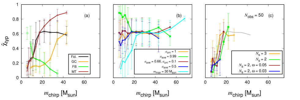
Figure 1.— The mean dimensionless total spin ${\bar{\chi}}_{\mathrm{typ}}$ as a function of $m_{\mathrm{chirp}}$ for models M1–M13 (Table 2). We use $N_{\mathrm{obs}}=10^{3}$ detectable mergers. In panels (b)–(c), the profiles for model M1 are presented by gray lines. Bars correspond to $1\sigma$ credible intervals.

Table 2 Properties of hierarchical mergers in our models. The first and second columns indicate the model number and its variation from the fiducial model (Table 1). The third and fourth columns show the fraction of high-g mergers among all and detectable mergers, respectively. The fifth column shows the maximum chirp mass ($m_{\mathrm{chirp,max}}$) among $N_{\mathrm{obs}}=10^{3}$ detectable mergers. The sixth and seventh columns show the average and the standard deviation of $\chi_{\mathrm{p}}$ among all merging pairs.

model	Parameter	high-g fraction	high-g detection fraction	$m_{\mathrm{chirp,max}}[{\rm M}_{\odot}]$	${\bar{\chi}}_{\mathrm{p}}$	$\sigma(\chi_{\mathrm{p}})$
M1	Fiducial	0.33	0.68	56	0.17	0.26
M2	Globular cluster (GC)	0.063	0.17	44	0.030	0.13
M3	Field binary (FB)	0	0	33	0	0
M4	Migration trap (MT)	0.31	0.80	42	0	0
M5	$a_{\mathrm{uni}}=1$	0.32	0.73	52	0.50	0.21
M6	$a_{\mathrm{ave}}=0.99$	0.31	0.70	51	0.75	0.20
M7	$a_{\mathrm{ave}}=0.66$, $a_{\mathrm{uni}}=0.1$	0.33	0.72	55	0.55	0.13
M8	$a_{\mathrm{ave}}=0.5$	0.33	0.74	65	0.46	0.12
M9	$m_{\mathrm{max}}=30\,{\rm M}_{\odot}$	0.35	0.73	70	0.18	0.26
M10	$N_{\mathrm{obs}}=50$, $N_{\mathrm{s}}=3$	0.25	0.62	28	0.13	0.24
M11	$N_{\mathrm{obs}}=50$, $N_{\mathrm{s}}=2$	0.15	0.28	24	0.077	0.19
M12	$N_{\mathrm{obs}}=50$, $N_{\mathrm{s}}=2$, $\omega=0.05$	0.077	0.18	19	0.040	0.14
M13	$N_{\mathrm{obs}}=50$, $N_{\mathrm{s}}=2$, $\omega=0.03$	0.046	0.14	19	0.023	0.11

3. Results

In § 3.1, we investigate characteristic features in hierarchical mergers, using our flexible tool (§ 2.2) to generate mock GW datasets for a large range of input parameter combinations. In $\S\,\ref{sec:results_ligo_data}$, we analyze GW data observed in LIGO/Virgo O1–O3a. We first derive signatures and properties of hierarchical mergers ($\S\,\ref{sec:result_rec_x_obs}$), using the simple fitting formula for spin vs. chirp mass (§ 2.3.1). We then assess ($\S\,\ref{sec:results_bayesian_factor}$) how well the predictions in our mock GW catalogs and in our physical AGN disk models (Tagawa et al., 2021b) in fact match these observed GW data. Finally, in $\S\,$3.3, we analyze mock GW data, and investigate how well the signatures of hierarchical models, described by the simple fitting formulae (${\bar{\chi}}_{\mathrm{typ}}$ vs. $m_{\mathrm{chirp}}$), can be recovered from future, larger GW catalogs.

3.1. Profiles for average spin parameters

3.1.1 Dependence on population parameters

We first show the parameter dependence of the ${\bar{\chi}}_{\mathrm{typ}}$ profile as a function of $m_{\mathrm{chirp}}$ using mock GW events, in which hierarchical mergers are assumed to be frequent. In Table 2, we list the model varieties we have investigated. These include the fiducial model (M1), and 12 different varieties (models M2–M13). We examine different choices of the initial spin magnitudes (models M5–M8) and the maximum mass of 1g BHs (model M9), the fraction of hierarchical mergers (models M10–M13), and the several parameter sets mimicking different populations (models M2–M4, Table 3). We also investigate a variety of additional models in the appendix (models M14–M28, Table 5).

Fig. 1 shows the profiles for models M1–M13 (Table 2). For models in which hierarchical mergers are frequent (panels (b) and (c) of Fig. 1 and Fig. 7), there are universal trends for hierarchical mergers in the ${\bar{\chi}}_{\mathrm{typ}}$ profiles: (i) increase (or decrease) of ${\bar{\chi}}_{\mathrm{typ}}$ to $\sim 0.6$ at low $m_{\mathrm{chirp}}$. (ii) plateau of ${\bar{\chi}}_{\mathrm{typ}}$ with $\sim 0.6$ at high $m_{\mathrm{chirp}}$. Thus, the profile is roughly characterized by two lines if hierarchical mergers are frequent, mergers originate mostly from one population, and the typical spin magnitude for 1g BHs does not depend on their masses. The profile of ${\bar{\chi}}_{\mathrm{typ}}$ strongly depends on $a_{\mathrm{ave}}$, $a_{\mathrm{uni}}$, and $m_{\mathrm{max}}$ (Fig. 1 b), while it is less affected by the other parameters (see Fig. 7).

The typical value of ${\bar{\chi}}_{\mathrm{typ}}\sim 0.6$ at the plateau can be understood as follows. When masses and spin magnitudes between the primary and secondary BHs are similar ($m_{\mathrm{1}}\sim m_{\mathrm{2}}$ and $a_{\mathrm{1}}\sim a_{\mathrm{2}}\sim a_{0}$) and the directions of BH spins are isotropic, the typical magnitude of mass-weighted BH spins is

$$|{\bm{a}}_{\mathrm{w}}|=\left\langle\left|\frac{m_{\mathrm{1}}{\bm{a}}_{\mathrm{1}}+m_{\mathrm{2}}{\bm{a}}_{\mathrm{2}}}{m_{\mathrm{1}}+m_{\mathrm{2}}}\right|\right\rangle\sim\frac{\sqrt{7}}{3}a_{0},$$ (30)

where $\langle\dots\rangle$ represents an average over the number of samples. If we approximate

$${\bar{\chi}}_{\mathrm{p}} \simeq\left\langle|{\bm{a}_{0}}||\mathrm{cos}\theta|\right\rangle\sim\frac{\pi}{4}a_{0},$$

$$\overline{|\chi_{\mathrm{eff}}|} \simeq\left\langle|{\bm{a}_{\mathrm{w}}}||\mathrm{sin}\theta|\right\rangle\sim\frac{1}{2}|{\bm{a}_{\mathrm{w}}}|,$$ (31)

then

$${\bar{\chi}}_{\mathrm{typ}} =\left(\overline{|\chi_{\mathrm{eff}}|}^{2}+{\bar{\chi}}_{\mathrm{p}}^{2}\right)^{1/2}$$

$$\sim\left[\left(\frac{\sqrt{7}}{3}\frac{1}{2}\right)^{2}+\left(\frac{\pi}{4}\right)^{2}\right]^{1/2}a_{0}\sim 0.90a_{0}.$$ (32)

Since merger remnants typically have spin magnitudes of $a_{0}\sim 0.7$ (Buonanno et al., 2008), ${\bar{\chi}}_{\mathrm{typ}}\sim 0.6$ for mergers among high-g BHs, which is roughly consistent with the value at the plateau (Figs. 1 and 7). Note that when $q\ll 1$, $|{\bm{a}}_{\mathrm{w}}|\sim a_{0}$ and so the average value is slightly enhanced to ${\bar{\chi}}_{\mathrm{typ}}\sim 0.93a_{0}$.

As $m_{\mathrm{max}}$ increases, the bending point between the two lines increases (gray and cyan lines in Fig. 1 b). This is because $m_{\mathrm{max}}$ determines the critical mass above which all merging BHs are of high generations with high spins of $\sim 0.7$. As the bending point is not influenced by the other parameters, the maximum mass of 1g BHs can be estimated from the bending point of the ${\bar{\chi}}_{\mathrm{typ}}$ profile. Note that since the bending points of the $\chi_{\mathrm{p}}$ and $\chi_{\mathrm{eff}}$ profiles are similar in shape to that of the $\chi_{\mathrm{typ}}$ profile for mergers with isotropic BH spins (Fig. 3 a), either $\chi_{\mathrm{typ}}$, $\chi_{\mathrm{p}}$ or $\chi_{\mathrm{eff}}$ can constrain the maximum mass of 1g BHs if the profiles are reconstructed well.

Additionally, $a_{\mathrm{ave}}$ and $a_{\mathrm{uni}}$ influence ${\bar{\chi}}_{\mathrm{typ}}$ at the smallest values of $m_{\mathrm{chirp}}$ (Fig. 1 b). This suggests that typical spin magnitudes of 1g BHs can be presumed by spins at small $m_{\mathrm{chirp}}$. However, note that ${\bar{\chi}}_{\mathrm{typ}}$ at small $m_{\mathrm{chirp}}$ is also influenced by the observational errors on $\chi_{\mathrm{p}}$ and $\chi_{\mathrm{eff}}$. Due to the smaller errors on $|\chi_{\mathrm{eff}}|$ compared to $\chi_{\mathrm{p}}$, $\overline{|\chi_{\mathrm{eff}}|}$ may constrain the typical spin values of 1g BHs more precisely using a number of events (green and orange lines in Fig. 3 a). Note that ${\bar{\chi}}_{\mathrm{p}}>\overline{|\chi_{\mathrm{eff}}|}$ when the BH spins are isotropic due to their definition. In model M7, the average and the dispersion of the spin magnitude for 1g BHs are set to be roughly the same as for the merger remnants. In such cases, the signatures of hierarchical mergers cannot be identified from the spin distributions (brown line in Fig. 1 b). Also, for models in which the typical spin magnitude for 1g BHs are close to $\sim 0.7$ (e.g. models M5 and M8), a large number of events are needed to detect the hierarchical merger signatures.

In Fig. 1 (c), we can see how the features for hierarchical mergers in the $\chi_{\mathrm{typ}}$ profile are influenced by the fraction of hierarchical mergers for $N_{\mathrm{obs}}=50$. The plateau at high $m_{\mathrm{chirp}}$ is seen for $N_{\mathrm{s}}=3$ (orange), while the rise of $\chi_{\mathrm{typ}}$ to $\sim 0.6$ at low $m_{\mathrm{chirp}}$ is seen for $N_{\mathrm{s}}=2$ with $\omega\geq 0.05$ (green and brown). These suggest that with $N_{\mathrm{obs}}=50$ the plateau and the rise of $\chi_{\mathrm{typ}}$ to $\sim 0.6$ can be confirmed when the detection fraction of mergers of high-g BHs roughly exceeds $\sim 0.5$ and $\sim 0.15$, respectively (models M10, M12, Table 2).

To summarize, the profile of ${\bar{\chi}}_{\mathrm{typ}}$ is mostly affected only by $a_{\mathrm{ave}}$, $a_{\mathrm{uni}}$, and $m_{\mathrm{max}}$, while the other parameters may affect the maximum $m_{\mathrm{chirp}}$ or the frequency of high-g mergers (Tables 2 and 5).

Table 3 Adopted parameter values for several populations. The differences with respect to the fiducial model (Table 1) are listed.

Globular cluster (GC)
1	$m_{\mathrm{max}}=45\,{\rm M}_{\odot}$
2	$N_{\mathrm{s}}=2$
3	$\omega=0.03$
4	$v_{\mathrm{esc}}=30\,\mathrm{km/s}$
Field binary (FB)
1	$m_{\mathrm{max}}=45\,{\rm M}_{\odot}$
2	$N_{\mathrm{s}}=1$
3	$\theta_{1}=\theta_{2}=0$
4	$a_{\mathrm{uni}}$ follows Eq. (37)
Migration trap (MT)
1	$\theta_{1}=\theta_{2}=0$

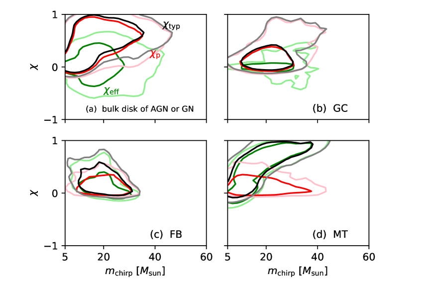
Figure 2.— The 90 (dark lines) and 99 (light lines) percentile distributions in the spin vs. $m_{\mathrm{chirp}}$ plane. Black, red, and green lines represent the distributions of $\chi_{\mathrm{typ}}$, $\chi_{\mathrm{p}}$, and $\chi_{\mathrm{eff}}$, respectively. Panels (a), (b), (c), and (d) show distributions for mergers in AGNs (bulk disks), GCs, FBs, and MTs, respectively.

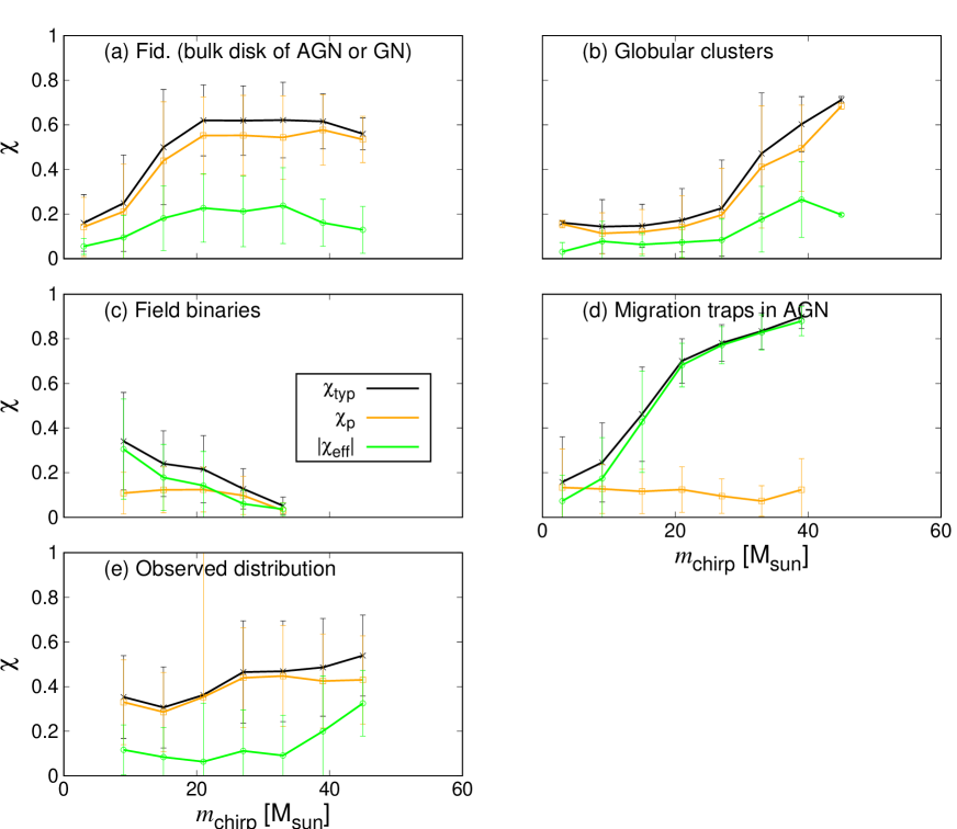
Figure 3.— The profiles for the average spin parameters as a function of $m_{\mathrm{chirp}}$ for $10^{3}$ detectable mergers. Black, orange, and green lines represent the average of $\chi_{\mathrm{typ}}$, $\chi_{\mathrm{p}}$, and $|\chi_{\mathrm{eff}}|$, respectively. Panels (a)–(e), respectively, present the distributions for mergers in AGN disks (M1), GCs (M2), FBs (M3), MTs (M4), and those observed by LIGO/Virgo O1–O3a. The averages for observed distributions (e) are calculated by averaging the medians of the parameters estimated in observed events. Bars correspond to $1\sigma$ credible intervals.

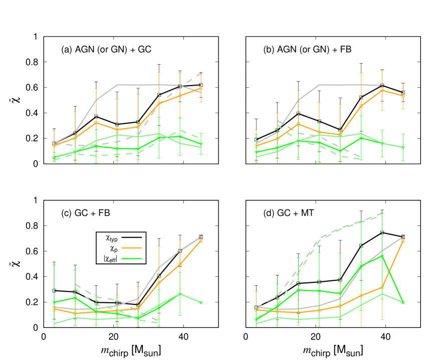
Figure 4.— Same as Fig. 3, but for mixture of two models. Both channels contribute to 1000 mergers, and contributing two models are specified in the upper left of each panel. ”AGN”, ”GC”, ”FB”, and ”MT” represent mergers in the AGN disks, GCs, FBs, and MTs, respectively. Thin and dashed lines present the $\chi_{\mathrm{eff}}$ and $\chi_{\mathrm{typ}}$ profiles only for the former and the latter populations in the legend, respectively.

3.1.2 Contribution from multiple populations

In the fiducial model (M1), the parameter values (Table 1) are roughly adjusted to reproduce properties of mergers in AGN disks outside of MTs (Tagawa et al., 2021b) or NSCs. The $\chi_{\mathrm{typ}}$ profile is similar but the $m_{\mathrm{chirp}}$ distribution is different between the fiducial model and physically motivated models derived in Tagawa et al. (2021b). The former is because the profile is characterized by the few parameters ($m_{\mathrm{max}}$, $a_{\mathrm{uni}}$, $a_{\mathrm{ave}}$) as found in $\S\,\ref{sec:result_profiles_mock}$, while the latter is because the $m_{\mathrm{chirp}}$ distributions are affected by how BHs pair with other BHs and merge in AGN disks.

In this section, we additionally consider the spin distributions for mergers typically expected in several environments, including GCs, FBs, and MTs of AGN disks. Values of the parameters adopted to mimic these populations are listed in Table 3. Figs. 2 and 3, and panel (a) in Fig. 1 present the distributions and the profiles of the spin parameters ($\chi_{\mathrm{typ}}$, $\chi_{\mathrm{p}}$, and $\chi_{\mathrm{eff}}$) as functions of $m_{\mathrm{chirp}}$ for these populations. Fig. 4 is the same as Fig. 3, but mergers are contributed by a mixture of two populations. Some contribution from multiple populations to the observed events is also favored by the analysis in Zevin et al. (2020b).

For mergers in GCs, we set lower escape velocity $v_{\mathrm{esc}}=30\,\mathrm{km/s}$, $N_{\mathrm{s}}=2$ and $\omega=0.03$ to reproduce the detection fraction of hierarchical mergers of $\sim 10$–$20\%$, which is predicted by theoretical studies (e.g. O’Leary et al., 2016; Rodriguez et al., 2019, Table 2). We chose higher $m_{\mathrm{max}}=45\,{\rm M}_{\odot}$ as GCs are composed of metal-poor stars (e.g. Peng et al., 2006; Leaman et al., 2013; Brodie et al., 2014); other parameters are the same as those for AGN disks. Note that $m_{\mathrm{max}}$ in metal-poor environments is uncertain due to uncertainties on the reaction rate of carbon burning (Farmer et al., 2019) and the enhancement of the helium core mass by rotational mixing (Chatzopoulos & Wheeler, 2012; Yoon et al., 2012; Vink et al., 2021).

Due to higher $m_{\mathrm{max}}$, ${\bar{\chi}}_{\mathrm{typ}}$ continues to increase until higher $m_{\mathrm{chirp}}$ (panel b in Fig. 3, see also Rodriguez et al. 2018) compared to the fiducial model (panel a). Also, 90 percentile regions are distributed around $\chi_{\mathrm{eff}}\sim 0$ and $\chi_{\mathrm{p}}\sim 0$ (Fig. 2 b) as a large fraction of mergers are among 1g BHs. Thus, the distribution of ${\bar{\chi}}_{\mathrm{typ}}$ at low $m_{\mathrm{chirp}}$ is clearly different between mergers in AGN disks and GCs, mainly due to the difference of $m_{\mathrm{max}}$ and the fraction of mergers among high-g BHs. If mergers are comparably contributed both by GCs and AGN disks, steep increase of ${\bar{\chi}}_{\mathrm{typ}}$ against $m_{\rm chirp}$ appears twice (panel a in Fig. 4). Thus, mixture of these populations can be discriminated by analyzing the spin distribution. Note that the intermediate line between the two increases in the ${\bar{\chi}}_{\mathrm{typ}}$ profile is roughly characterized by the ratio of mergers from AGN disks and GCs. Hence, the contribution from multiple populations would be distinguishable by analyzing the profile by using a number of GW events.

For mergers among FBs, we set $N_{\mathrm{s}}=1$ and $m_{\mathrm{max}}=45\,{\rm M}_{\odot}$. Although BH spin distributions are highly uncertain, we refer to Bavera et al. (2019) who proposed that ${\bar{\chi}}_{\mathrm{eff}}$ is high at low $m_{\mathrm{chirp}}$ of $\lesssim 10-20\,{\rm M}_{\odot}$ as low-mass progenitors have enough time to be tidally spun up. We assume that $a_{\mathrm{uni}}$ follows

$$a_{\mathrm{uni}}=\left\{\begin{array}[]{l}1~{}~{}\mathrm{for}~{}~{}~{}m_{\mathrm{1g}}\leq 15\,{\rm M}_{\odot}\\ (30\,{\rm M}_{\odot}-m_{\mathrm{1g}})/15\,{\rm M}_{\odot}\\ ~{}~{}~{}~{}~{}~{}~{}~{}~{}~{}~{}~{}\mathrm{for}~{}~{}~{}15\,{\rm M}_{\odot}\leq m_{\mathrm{1g}}\leq 30\,{\rm M}_{\odot}\\ 0~{}~{}\mathrm{for}~{}~{}~{}30\,{\rm M}_{\odot}\leq m_{\mathrm{1g}}.\end{array}\right.$$ (37)

BH spins are assumed to be always aligned with the orbital angular momentum of binaries, although we do not always expect spins to be aligned (e.g. Kalogera, 2000; Rodriguez et al., 2016b). In such a setting, $\overline{|\chi_{\mathrm{eff}}|}$ decreases as $m_{\mathrm{chirp}}$ increases (panels c of Figs. 2 and 3). Also, non-zero $\chi_{\mathrm{p}}$ is due to assumed observational errors (orange line in Fig. 3 c). The profile expected for the binary evolution channel is significantly different from those expected for the other channels. If mergers arise comparably from FBs and GCs, $\overline{|\chi_{\mathrm{eff}}|}$ exceeds ${\bar{\chi}}_{\mathrm{p}}$ at low $m_{\mathrm{chirp}}$ (panel c of Fig. 4). As contribution from mergers in FBs enhances $\overline{|\chi_{\mathrm{eff}}|}$ relative to ${\bar{\chi}}_{\mathrm{p}}$ at low $m_{\mathrm{chirp}}$, we could constrain the contribution from FBs using the ratio of $\overline{|\chi_{\mathrm{eff}}|}$ to ${\bar{\chi}}_{\mathrm{p}}$. Observed events so far suggest that $|\chi_{\mathrm{eff}}|$ is typically lower than $\chi_{\mathrm{p}}$ at low $m_{\mathrm{chirp}}$ (panel e of Fig. 3), implying that the contribution to the observed mergers from FBs is minor, unless adopted spins for 1g BHs need significant revisions.

For mergers in MTs, we assume that parameters are the same as in the fiducial model (Table 1), while BH spins are always aligned with the orbital angular momentum of the binaries. Such alignment is expected for binaries in MTs where randomization of the binary orbital angular momentum directions by binary-single interactions is inefficient due to rapid hardening and merger caused by gas dynamical friction (unlike in gaps formed further out in the disk, where these interactions were found to be very important by Tagawa et al. 2020a), and so the BH spins are aligned with circumbinary disks due to the Bardeeen-Petterson effect (Bardeen & Petterson, 1975), and circumbinary disks are aligned with the binaries due to viscous torque (e.g. Moody et al., 2019). Here, we assume that the orbital angular momentum directions of binaries are the same as that of the AGN disk referring to Lubow et al. (1999), which is different from the assumption (anti-alignment with $50\%$) adopted in Yang et al. (2019). In this model, the $\chi_{\mathrm{p}}$ and $|\chi_{\mathrm{eff}}|$ distributions are significantly different from those in the other models (panels d of Figs. 2 and 3). The value of $\chi_{\mathrm{eff}}$ at high $m_{\mathrm{chirp}}$ is typically high, while $\chi_{\mathrm{p}}$ is low. When mergers originate comparably in MTs and GCs, $\overline{|\chi_{\mathrm{eff}}|}$ significantly exceeds ${\bar{\chi}}_{\mathrm{p}}$ in a wide range of $m_{\mathrm{chirp}}$ (Fig. 4 d). As $\overline{|\chi_{\mathrm{eff}}|}$ is typically lower than ${\bar{\chi}}_{\mathrm{p}}$ in the observed events in all $m_{\mathrm{chirp}}$ bins (Fig. 4 e), the contribution from MTs to the detected mergers is probably minor.

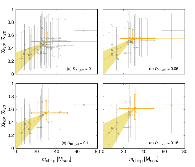
Figure 5.— The ${\bar{\chi}}_{\mathrm{typ}}$ profile as a function of $m_{\mathrm{chirp}}$ constructed using the GW data observed in LIGO/Virgo O1–O3a. Orange line presents the recovered profile using the model described in $\S\,\ref{sec:method_reconstruction_spin}$ (Eq. 19). Bars and shaded regions represent $1\sigma$ credible intervals for ${\bar{\chi}}_{\mathrm{typ}}$ at the plateau $b_{\mu}$, the critical chirp mass at the bending point of the profile $m_{\mathrm{crit}}$, and the slope of the ${\bar{\chi}}_{\mathrm{typ}}$ at a lower chirp mass $a_{\mu}$. Panels (a), (b), (c), and (d) presents results for events with $D_{\mathrm{KL}}\geq$ 0, 0.05, 0.1, and 0.15, respectively. Gray plots are the same as those in Fig. 8 (c).

3.2. Application to LIGO/Virgo O1–O3a data

3.2.1 Reconstruction of spin profiles

We analyze the GW data observed in LIGO/Virgo O1–O3a reported by Abbott et al. (2019) and Abbott et al. (2020b). Although $\chi_{\mathrm{p}}$ and $\chi_{\mathrm{typ}}$ suffer large uncertainties (e.g. Fig. 8), their median values indicate a positive correlation with $m_{\mathrm{chirp}}$. Such positive correlation is, if confirmed, consistent with the growth of BH spin magnitudes by hierarchical mergers as presented in Figs. 1, 3, and 7.

To confirm the features in the $\chi$-profiles due to hierarchical mergers, we reconstruct the ${\bar{\chi}}_{\mathrm{typ}}$ profile from the observed GW data in the way described in $\S\,\ref{sec:method_reconstruction_spin}$. We discretize the posteriors for $m_{\rm chirp}$, $\chi_{\rm eff}$, and $\chi_{\rm p}$ with 20, 40, and 20 bins in the ranges from the minimum to the maximum of posteriors for $m_{{\rm chirp},i}$, from -1 to 1, and from 0 to 1, respectively. Note that the prior and posterior distributions for some events are similar to each other, which means that $\chi_{\mathrm{p}}$ is less constrained by the waveforms. To exclude events in which $\chi_{\mathrm{p}}$ are not well estimated, we only use events in which the Kullback-Leibler (KL) divergence between prior and posterior samples evaluated using heuristic estimates of $\chi_{\mathrm{p}}$ ($D_{\mathrm{KL}}$) exceeds a critical value of $D_{\mathrm{KL,cri}}=0$, 0.05, 0.1, 0.15, or 0.2. We consider that $\chi_{\mathrm{p}}$ for events with non-zero $D_{\mathrm{KL}}$ is statistically useful to understand the spin distribution. We use the events with $m_{2}\geq 5\,{\rm M}_{\odot}$ provided in LIGO Scientific Collaboration & Virgo Collaboration (2020) and LIGO Scientific Collaboration & Virgo Collaboration (2021) as we do not model mergers of neutron stars. Then, the number of events with $D_{\mathrm{KL}}\geq 0$, 0.05, 0.1, 0.15, and 0.2 are 44, 28, 20, 12, and 7, respectively. We present $1\sigma$ errors on the estimated parameters below unless stated otherwise.

The reconstructed ${\bar{\chi}}_{\mathrm{typ}}$ profiles for $D_{\mathrm{KL,cri}}=0$, 0.05, 0.1, and 0.15 are, respectively, presented by orange lines in panels (a)–(d) of Fig. 5, and the posterior distributions and correlations of the reconstructed parameters for $D_{\mathrm{KL,cri}}=0$ are presented in Fig. 10 in the Appendix. For $D_{\mathrm{KL,cri}}=0$, 0.05, 0.1, 0.15, and 0.20, respectively, ${\bar{\chi}}_{\mathrm{typ}}$ at the plateau is $b_{\mu}=0.51^{+0.14}_{-0.07}$, $0.55^{+0.14}_{-0.08}$, $0.55^{+0.19}_{-0.11}$, $0.62^{+0.22}_{-0.23}$, and $0.66^{+0.20}_{-0.18}$, the critical chirp mass at the bending point of the ${\bar{\chi}}_{\mathrm{typ}}$ profile is $m_{\mathrm{crit}}=31^{+23}_{-15}\,{\rm M}_{\odot}$, $29^{+21}_{-12}\,{\rm M}_{\odot}$, $30^{+21}_{-14}\,{\rm M}_{\odot}$, $31^{+18}_{-15}\,{\rm M}_{\odot}$, and $36^{+17}_{-16}\,{\rm M}_{\odot}$, and the slope of ${\bar{\chi}}_{\mathrm{typ}}$ at $m_{\mathrm{chirp}}<m_{\mathrm{crit}}$ is $a_{\mu}=10^{+7}_{-4}\times 10^{-3}\,{\rm M}_{\odot}^{-1}$, $12^{+8}_{-5}\times 10^{-3}\,{\rm M}_{\odot}^{-1}$, $12^{+7}_{-6}\times 10^{-3}\,{\rm M}_{\odot}^{-1}$, $15^{+12}_{-7}\times 10^{-3}\,{\rm M}_{\odot}^{-1}$, and $15^{+8}_{-6}\times 10^{-3}\,{\rm M}_{\odot}^{-1}$. To understand the influence of GW190521, which seems to have a large impact on spin distributions due to its large mass and $\chi_{\rm p}$, we repeated our analysis excluding this event. In this case, for $D_{\mathrm{KL,cri}}=0$, 0.05, and 0.1, respectively, $b_{\mu}=0.50^{+0.15}_{-0.07}$, $0.52^{+0.14}_{-0.08}$, and $0.59^{+0.24}_{-0.14}$, $m_{\mathrm{crit}}=36^{+19}_{-14}\,{\rm M}_{\odot}$, $25^{+23}_{-11}\,{\rm M}_{\odot}$, and $37^{+19}_{-17}\,{\rm M}_{\odot}$, and $a_{\mu}=8^{+4}_{-4}\times 10^{-3}\,{\rm M}_{\odot}^{-1}$, $12^{+10}_{-6}\times 10^{-3}\,{\rm M}_{\odot}^{-1}$, and $12^{+4}_{-5}\times 10^{-3}\,{\rm M}_{\odot}^{-1}$, while for $D_{\mathrm{KL,cri}}=0.15$ and $0.2$, the parameters are not well determined due to the small number of events. For $D_{\rm LK,crit}\leq 0.1$, the evaluated values of the parameters are similar with and without GW190521.

The positive value of the slope ($a_{\mu}$), i.e., the increase of ${\bar{\chi}}_{\mathrm{typ}}$ at low $m_{\mathrm{chirp}}$ is confirmed with $\gtrsim 2\sigma$ confidence, which is a tell-tale sign of frequent hierarchical mergers. Also, according to the analysis in $\S\,\ref{sec:result_profiles_mock}$, the detection of the rise of ${\bar{\chi}}_{\mathrm{typ}}$ at low $m_{\mathrm{chirp}}$ with $N_{\mathrm{obs}}=50$ roughly requires that the detection fraction of mergers of high-g BHs exceeds $\sim 0.15$. As the number of events is smaller than 50 (e.g. $N_{\mathrm{obs}}=28$ for $D_{\mathrm{KL,cri}}=0.05$), the high-g detection fraction would be even higher than $\sim 0.15$. Thus, hierarchical mergers are preferred from the analysis. Note that accretion can also produce a positive correlation, but $|\chi_{\mathrm{eff}}|>\chi_{\mathrm{p}}$ is predicted in such cases, similarly to mergers in MTs (panel d of Fig. 3). As $|\chi_{\mathrm{eff}}|<\chi_{\mathrm{p}}$ is predicted by GW observations (panel e of Fig. 3), accretion is disfavored as a process enhancing the BH spin magnitudes.

For $D_{\mathrm{KL,cri}}=$ 0.05, 0.1, 0.15, and 0.20 (panels b, c, and d of Fig. 5), the value of ${\bar{\chi}}_{\mathrm{typ}}$ at the plateau ($b_{\mu}\sim 0.6$) is consistent with that expected from hierarchical mergers ($\sim 0.6$), which possibly supports frequent hierarchical mergers with the high-g detection fraction to be $\gtrsim 0.5$ ($\S\,$3.1.1). On the other hand, for $D_{\mathrm{KL,cri}}=0$, $b_{\mu}\sim 0.5$, which is somewhat lower than the expected value of $0.6$. This is presumably because $\chi_{\mathrm{p}}$ values for events with $D_{\mathrm{KL}}\leq 0.05$ are not well constrained and just reflect assumed priors. Also, note that events with high $\chi_{\mathrm{p}}$ might tend to be missed as the waveform for large $\chi_{\mathrm{p}}$ (Apostolatos et al., 1994; Kidder, 1995; Pratten et al., 2020) or spin (Kesden et al., 2010; Gerosa et al., 2019) mergers often accompany strong amplitude modulation, reducing SNRs.

Here, ${\bar{\chi}}_{\mathrm{typ}}$ at $m_{\mathrm{chirp}}=m_{\mathrm{min}}$ is closely related to the typical spin magnitude for 1g BHs (Fig. 1 b). If we assume the median values for ${\bar{\chi}}_{\mathrm{typ}}$ and $m_{\mathrm{crit}}$, ${\bar{\chi}}_{\mathrm{typ}}$ at $m_{\mathrm{chirp}}=5\,{\rm M}_{\odot}$ is $0.26^{+0.10}_{-0.18}$, $0.27^{+0.12}_{-0.20}$, $0.26^{+0.14}_{-0.19}$, $0.23^{+0.18}_{-0.32}$, and $0.29^{+0.20}_{-0.25}$ for $D_{\mathrm{KL,cri}}=0$, 0.05, 0.1, 0.15, and 0.20, respectively. These suggest that 1g BHs typically have $a\lesssim 0.4$. Since this value is effectively enhanced by the observational errors on ${\bar{\chi}}_{\mathrm{p}}$, the estimated typical spin magnitude of 1g BHs is still consistent with $\sim 0$ as predicted by stellar evolution models (Fuller & Ma, 2019), which is also verified later ($\S\,$3.3).

The critical chirp mass at the bending point of the ${\bar{\chi}}_{\mathrm{typ}}$ profile ($m_{\mathrm{crit}}$) is related to the maximum mass of 1g BHs (Fig. 1 f). The analysis loosely constrains the parameter to $m_{\mathrm{crit}}\sim 15$–$50\,{\rm M}_{\odot}$, from which we discuss in $\S\,\ref{sec:result_rec_x}$ that the maximum mass of 1g BHs is estimated to be $\sim 20$–$60\,{\rm M}_{\odot}$. However, it needs a caution that $m_{\mathrm{crit}}$ is restricted from $5\,{\rm M}_{\odot}$ to the maximum chirp mass among the event ($\sim 67\,{\rm M}_{\odot}$) in this analysis, which may artificially produce the bending point and the plateau. To confidently confirm the plateau, $m_{\mathrm{crit}}$ needs to be precisely constrained compared to the allowed range for $m_{\mathrm{crit}}$ of $5$–$67\,{\rm M}_{\odot}$, which would require further events (see also $\S\,\ref{sec:result_rec_x}$).

Table 4 The parameters of model A which are different from each population model (shown in Table 3) and the logarithm of their Bayes factor $K_{\mathrm{A,B}}$ relative to the fiducial model (”B”). The Bayes factors for the three parameters with $D_{\mathrm{KL,cri}}=0$, 0.05, 0.1, 0.15, and 0.2, and that for the two parameters are presented from the second to seventh columns. We highlight the models with positive Bayes factors in the five rightmost columns in boldface.

Parameters	$\mathrm{log}_{10}K_{\mathrm{A,B}}$ in 3D					$\mathrm{log}_{10}K_{\mathrm{A,B}}$ in 2D
	$D_{\mathrm{KL,cri}}=0$	$D_{\mathrm{KL,cri}}=0.05$	$D_{\mathrm{KL,cri}}=0.1$	$D_{\mathrm{KL,cri}}=0.15$	$D_{\mathrm{KL,cri}}=0.2$	-
AGN disk or NSC
$m_{\mathrm{max}}=15\,{\rm M}_{\odot}$	-6.9	-4.0	-1.8	-3.0	-1.5	-7.2
$m_{\mathrm{max}}=25\,{\rm M}_{\odot}$	1.3	-0.05	-1.1	-0.31	-0.27	1.3
$m_{\mathrm{max}}=30\,{\rm M}_{\odot}$	-0.9	-2.0	-2.7	-1.4	-0.90	0.085
$m_{\mathrm{max}}=35\,{\rm M}_{\odot}$	-3.2	-3.7	-4.6	-2.4	-1.6	-1.8
$m_{\mathrm{max}}=45\,{\rm M}_{\odot}$	-8.2	-7.6	-7.4	-4.2	-2.6	-5.7
$\alpha=2$	-0.065	0.35	0.65	0.065	0.29	-0.56
$\alpha=2$, $m_{\mathrm{max}}=15\,{\rm M}_{\odot}$	-12	-8.3	-4.5	-4.1	-3.3	-15
$\alpha=2$, $m_{\mathrm{max}}=25\,{\rm M}_{\odot}$	1.5	0.83	0.14	-0.060	0.13	1.4
$\alpha=2$, $m_{\mathrm{max}}=30\,{\rm M}_{\odot}$	1.4	0.12	-1.0	-0.58	-0.33	1.9
$\alpha=2$, $m_{\mathrm{max}}=35\,{\rm M}_{\odot}$	0.11	-1.1	-2.0	-1.2	-0.57	0.72
$\alpha=2$, $m_{\mathrm{max}}=45\,{\rm M}_{\odot}$	-2.7	-3.1	-3.4	-2.0	-0.87	-1.3
$a_{\mathrm{uni}}=1$	-2.2	-1.7	-2.1	-1.7	-1.0	-1.3
$a_{\mathrm{ave}}=0.3$	0.51	0.53	0.042	-0.21	0.062	-0.035
$a_{\mathrm{ave}}=0.5$	-1.5	-0.85	-1.2	-1.2	-0.67	-1.1
$a_{\mathrm{ave}}=0.7$	-5.5	-4.1	-4.3	-3.0	-2.0	-2.4
$\sigma_{\mathrm{p}}=0.3$	-0.021	0.053	-0.059	-0.15	-0.16	-0.24
$\sigma_{\mathrm{p}}=0.4$	0.37	0.42	-0.075	-0.20	-0.072	0.40
$v_{\mathrm{esc}}=30\,\mathrm{km/s}$	-14	-8.7	-6.0	-5.7	-5.7	-13
$w=0.03$	-26	-23	-12	-13	-8.3	-30
$w=0.2$	-3.2	-2.4	-3.1	-1.8	-0.81	-2.1
$\gamma_{\mathrm{t}}=0$	-21	-16	-11	-11	-8.2	-25
$\gamma_{\mathrm{t}}=4$	-3.7	-2.8	-3.1	-1.7	-0.64	-3.2
$\gamma_{\mathrm{q}}=0$	-6.5	-4.5	-2.3	-2.8	-2.0	-6.7
$\gamma_{\mathrm{q}}=4$	0.39	0.12	-0.26	-0.18	-0.058	0.64
$N_{\mathrm{s}}=2$	-49	-31	-25	-29	-25	-48
$N_{\mathrm{s}}=2$, $m_{\mathrm{max}}=30\,{\rm M}_{\odot}$	-0.55	-3.3	-5.7	-2.9	-4.0	-0.84
$N_{\mathrm{s}}=2$, $m_{\mathrm{max}}=45\,{\rm M}_{\odot}$	-3.6	-6.1	-7.9	-3.9	-3.6	-0.95
$N_{\mathrm{s}}=2$, $m_{\mathrm{max}}=60\,{\rm M}_{\odot}$	-14	-13	-12	-6.9	-5.0	-9.5
$N_{\mathrm{s}}=3$	-4.1	-3.0	-1.5	-1.8	-2.0	-5.9
$N_{\mathrm{s}}=3$, $m_{\mathrm{max}}=25\,{\rm M}_{\odot}$	1.0	-0.55	-1.2	-0.56	-0.77	0.81
$N_{\mathrm{s}}=3$, $m_{\mathrm{max}}=30\,{\rm M}_{\odot}$	1.9	-0.11	-1.7	-0.61	-0.77	2.1
$N_{\mathrm{s}}=3$, $m_{\mathrm{max}}=35\,{\rm M}_{\odot}$	0.24	-2.1	-3.8	-1.8	-1.5	1.3
$N_{\mathrm{s}}=3$, $m_{\mathrm{max}}=45\,{\rm M}_{\odot}$	-6.7	-7.2	-7.7	-4.2	-2.9	-3.7
$N_{\mathrm{s}}=5$	0.084	0.16	-0.50	-0.48	0.14	0.44
$N_{\mathrm{s}}=5$, $m_{\mathrm{max}}=15\,{\rm M}_{\odot}$	-0.96	-0.17	-0.091	-0.76	-0.065	-0.68
$N_{\mathrm{s}}=5$, $m_{\mathrm{max}}=30\,{\rm M}_{\odot}$	-3.6	-3.4	-3.8	-2.1	-1.1	-2.6
$N_{\mathrm{s}}=5$, $m_{\mathrm{max}}=45\,{\rm M}_{\odot}$	-11	-8.5	-7.8	-4.5	-2.4	-7.9
$N_{\mathrm{s}}=6$	-2.8	-2.0	-2.6	-1.5	-0.42	-2.0
Globular cluster
Fiducial	-2.3	-6.8	-8.7	-5.3	-4.8	-0.83
$\alpha=2$	4.2	-0.50	-1.5	-1.4	-2.1	5.8
$m_{\mathrm{max}}=30\,{\rm M}_{\odot}$	-12	-10	-8.7	-9.1	-7.0	-15
$a_{\mathrm{uni}}=1$	-12	-13	-16	-8.9	-9.6	-10
$a_{\mathrm{ave}}=0.3$	-0.84	-5.1	-7.8	-4.8	-5.2	-3.3
$a_{\mathrm{ave}}=0.5$	-1.8	-5.0	-8.6	-4.6	-4.6	-4.2
$a_{\mathrm{ave}}=0.7$	-12	-12	-14	-8.7	-7.9	-8.7
$v_{\mathrm{esc}}=100\,\mathrm{km/s}$	-3.1	-7.1	-8.5	-4.8	-4.9	-1.4
$w=0.05$	-2.1	-5.4	-7.1	-3.8	-3.9	0.54
$w=0.1$	-3.3	-5.5	-7.3	-4.1	-3.5	-0.72
$\alpha=2$, $a_{\mathrm{uni}}=1$	-4.1	-4.8	-5.6	-5.6	-4.8	-2.6
$\alpha=2$, $a_{\mathrm{ave}}=0.3$	4.9	0.38	-0.72	-1.1	-2.4	2.6
$\alpha=2$, $a_{\mathrm{ave}}=0.5$	0.15	-2.9	-5.0	-4.4	-4.6	-2.3
Field binary
Fiducial	-18	-17	-19	-12	-10	-9.1
Migration trap
Fiducial	-61	-37	-23	-17	-14	-57
AGN disk (Tagawa et al., 2021b)
$f_{\mathrm{m1g}}=1$	-4.0	-2.5	-1.6	-1.5	-0.63	-3.9
$f_{\mathrm{m1g}}=1.33$	-2.7	-1.9	-1.5	-0.53	-0.19	-2.5
$f_{\mathrm{m1g}}=1.66$	-2.0	-1.8	-1.8	-0.45	-0.16	-2.0
$f_{\mathrm{m1g}}=2$	1.1	0.032	-0.79	-0.15	0.045	1.2
$f_{\mathrm{m1g}}=3$	2.1	-0.19	-1.7	-1.7	-1.1	4.3

3.2.2 Bayes factors on spins and mass distributions

In the previous section we focus on the ${\bar{\chi}}_{\mathrm{typ}}$ profile, while here we use the distributions of $\chi_{\mathrm{eff}}$, $\chi_{\mathrm{p}}$, and $m_{\mathrm{chirp}}$ and discuss the preferred values for underlying parameters ${\bm{\lambda}}_{0}$.

To assess the relative likelihood to produce each event in different models, we calculate the Bayes factors between pairs of models,

$$K_{\mathrm{A,B}}=\frac{P({\bm{d}}|A)}{P({\bm{d}}|B)}$$ (38)

where

$$P({\bm{d}}|A)=\prod_{i}P({\bm{d}}_{i}|A),$$ (39)

$P({\bm{d}}_{i}|A)$ is the likelihood of obtaining data ${\bm{d}}_{i}$ observed in the GW event $i$ from model $A$,

$$P({\bm{d}}_{i}|A)=$$

$$\int P({\bm{d}}_{i}|m_{\mathrm{chirp}},\chi_{\mathrm{eff}},\chi_{\mathrm{p}}) P(m_{\mathrm{chirp}},\chi_{\mathrm{eff}},\chi_{\mathrm{p}}|A)$$

$$dm_{\mathrm{chirp}}d\chi_{\mathrm{eff}}d\chi_{\mathrm{p}}$$ (40)

and $P(m_{\mathrm{chirp}},\chi_{\mathrm{eff}},\chi_{\mathrm{p}}|A)$ is the probability distribution of $m_{\mathrm{chirp}}$, $\chi_{\mathrm{eff}}$, and $\chi_{\mathrm{p}}$ in model $A$. We calculate the three dimensional likelihood $P({\bm{d}}_{i}|m_{\mathrm{chirp}},\chi_{\mathrm{eff}},\chi_{\mathrm{p}})$ for the events.

We calculate the Bayes factors for events with $D_{\mathrm{KL}}\geq D_{\mathrm{KL,crit}}=0$, 0.05, 0.1, 0.15, and 0.2. We consider $D_{\mathrm{KL,crit}}=0.05$ as the fiducial value, and mostly discuss the Bayes factors for $D_{\mathrm{KL,crit}}=0.05$ below. Note that the events with positive Bayes factors for $D_{\mathrm{KL,crit}}=0.1$, $0.15$, or $0.2$ always have positive Bayes factors also for $D_{\mathrm{KL,crit}}=0.05$ somewhat incidentally.

To calculate $P(m_{\mathrm{chirp}},\chi_{\mathrm{eff}},\chi_{\mathrm{p}}|A)$, we first count mergers in $30\times 30\times 30$ uniform bins in $\chi_{\mathrm{eff}}$, $m_{\mathrm{chirp}}$, and $\chi_{\mathrm{p}}$ for model $A$. The maximum and minimum values of $m_{\mathrm{chirp}}$ for the bins are set to $100$ and $5\,{\rm M}_{\odot}$, respectively. In this section, we generate 1000 mergers for each model. To include error distributions for the variables ($m_{\mathrm{chirp}}$, $\chi_{\mathrm{eff}}$, $\chi_{\mathrm{p}}$) to $P(m_{\mathrm{chirp}},\chi_{\mathrm{eff}},\chi_{\mathrm{p}}|A)$, we sample 10 different realizations for each merger event predicted by the model. To reduce the statistical fluctuation in the distribution of $\chi_{\mathrm{eff}}$, $m_{\mathrm{chirp}}$, and $\chi_{\mathrm{p}}$ due to the finite number of mergers in our models, we perform a kernel-density estimate for the distribution using Gaussian kernels whose bandwidth is chosen to satisfy the Scott’s Rule (Scott, 1992). We calculate $P({{\bm{d}}_{i}}|m_{\mathrm{chirp}},\chi_{\mathrm{eff}},\chi_{\mathrm{p}})$ by means of 300 samples generated according to the observed posterior distributions as used in the previous section.

For reference, we also calculate the Bayes factors for the two parameters, $m_{\mathrm{chirp}}$ and $\chi_{\mathrm{eff}}$, using the 44 events used in the analysis with $D_{\rm KL}\geq 0$ in the previous section.

Table 4 lists the Bayes factors for some models relative to the fiducial model ($=B$, Table 1). The Bayes factors suggest that, compared to the $m_{\mathrm{chirp}}$, $\chi_{\mathrm{eff}}$, and $\chi_{\mathrm{p}}$ distributions typically expected for mergers in FBs and MTs (Table 3), the observed distribution is much more consistent with those in AGN disks. This is because high $|\chi_{\mathrm{eff}}|$ and low $\chi_{\mathrm{p}}$ expected for mergers either in FBs or MTs (panels c and d in Figs. 2 and 3) are incompatible with the observed distribution of $|\chi_{\mathrm{eff}}|<\chi_{\mathrm{p}}$ (Fig. 3 e).

For mergers in GCs, the models with small spin magnitudes for 1g BHs are less favored. This is presumably because infrequent hierarchical mergers ($\lesssim 20\%$) in GCs are difficult to explain typically high values of $\chi_{\mathrm{p}}$ if 1g BHs have low spin magnitudes. On the other hand, for $a_{\mathrm{ave}}=0.3$ and $\alpha=2$, the Bayes factor for $D_{\mathrm{KL,crit}}=0.05$ is as high as $\sim 10^{0.4}$. Thus, if mergers originate from GCs, 1g BHs are favored to have high spin magnitudes and follow a bottom heavy initial mass function.

For mergers in AGN disks or NSCs, the models with non-zero values for initial BH spins ($a_{\mathrm{ave}}=0.3$) as well as a high value for $\sigma_{\chi_{\mathrm{p}}}(\sim 0.3$–$0.4$) have high Bayes factors of $10^{0.5}$ and $10^{0.05}$–$10^{0.4}$ for $D_{\mathrm{KL,crit}}=0.05$, respectively. This is because non-zero ${\bar{\chi}}_{\mathrm{typ}}$ at low $m_{\mathrm{chirp}}$ in the observed distribution (Fig. 8) can be explained by adjusting these variables (Fig. 1). Also, large values for $\alpha$, which effectively shift the $\chi_{\mathrm{typ}}$ and $m_{\mathrm{chirp}}$ distribution toward lower $m_{\mathrm{chirp}}$, and accordingly raises ${\bar{\chi}}_{\mathrm{typ}}$ at low $m_{\mathrm{chirp}}$ (e.g. Fig. 7 e). This is presumably the reason why the model with $\alpha(=2)$ has a high Bayes factor of $10^{0.8}$ at $m_{\mathrm{max}}\sim 25\,{\rm M}_{\odot}$ compared to the models with $\alpha=1$ ($K_{A,B}\lesssim 1$).

Preferred values for $m_{\mathrm{max}}$ are probably as low as $\sim 15$–$30\,{\rm M}_{\odot}$ if the typical spin magnitude for 1g BHs is low. For $\alpha=1$, in the models with $N_{\mathrm{s}}=3$, 4, and 5, respectively, $m_{\mathrm{max}}=25$–$30\,{\rm M}_{\odot}$, $m_{\mathrm{max}}=20$–$25\,{\rm M}_{\odot}$, and $m_{\mathrm{max}}=15$–$20\,{\rm M}_{\odot}$ is preferred. The difference in preference of $m_{\mathrm{max}}$ for different $N_{\mathrm{s}}$ is because both variables are constrained by the maximum $m_{\mathrm{chirp}}$ among the GW events. In any case, the preferred values of $m_{\mathrm{max}}=15$–$30\,{\rm M}_{\odot}$ are roughly consistent with the values estimated in the previous section.

We also compare the properties inferred from GW observations with those predicted for mergers in AGN disks, which are calculated from one-dimensional $N$-body simulations, combined with a semi-analytical model used in Tagawa et al. (2021b). We adopt the fiducial model in Tagawa et al. (2021b), while we investigate several variations in which the initial BH masses are multiplied by $f_{\mathrm{m1g}}=$1, 1.33, 1.66, 2, and 3 so that $m_{\mathrm{max}}=15$, 20, 25, 30, and 45 ${\rm M}_{\odot}$, respectively. Since 1g BH masses are $5$–$15\,{\rm M}_{\odot}$ in the fiducial model, the minimum BH mass is given by $5f_{\mathrm{m1g}}\,{\rm M}_{\odot}$, in which the minimum chirp mass is $\sim 8.7f_{\mathrm{m1g}}\,{\rm M}_{\odot}$. To eliminate a reduction of the likelihood due to the lack of 1g BHs in the low mass ranges, we here calculate Bayes factors only using events with $m_{\mathrm{chirp}}\geq 8.7f_{\mathrm{m1g}}\,{\rm M}_{\odot}$. The errors on $m_{\mathrm{chirp}}$, $\chi_{\mathrm{eff}}$, and $\chi_{\mathrm{p}}$ are simply given by the normal distribution with the standard deviation of $0.08\,m_{\mathrm{chirp}}$, $0.12$, and $0.2$, respectively. The Bayes factors are listed in the bottom five rows in Table 4, which indicate that $m_{\mathrm{max}}\sim 30\,{\rm M}_{\odot}$ ($f_{\mathrm{m1g}}=2$) is preferred. Thus, the properties predicted for AGN disk-assisted mergers are likely to be consistent with the observed properties of the GW events.

Here, events with high Bayes factors for $D_{\mathrm{KL,crit}}=0.05$ tend to have high Bayes factors for the two dimensional likelihood (bold number in the third and rightmost columns of Table 4). We consider that this fact would further support the preferred models discussed above.

Overall, our analyses suggest that $m_{\mathrm{max}}=15$–$30\,{\rm M}_{\odot}$ with a high fraction of hierarchical mergers, or high spin magnitudes of $\sim 0.3$ for 1g BHs is favored. The former may support mergers in NSCs including AGN disks, while the latter may be consistent with those in GCs. Further events would be required to assess these possibilities in more detail.

We also discuss the spin distribution suggested in The LIGO Scientific Collaboration et al. (2020c). First, we compare the average and the standard deviation of $\chi_{\mathrm{p}}$ predicted by models and those estimated from LIGO/Virgo O1–O3a data. By analyzing the observed GW data, The LIGO Scientific Collaboration et al. (2020c) estimated that the average and the standard deviation of $\chi_{\mathrm{p}}$ are $0.21^{+0.15}_{-0.14}$ and $0.09^{+0.21}_{-0.07}$, respectively, assuming a truncated mass model. These values are consistent with models in which hierarchical mergers are frequent such as models M1, M9–M11 (Table 2), M18–M21, M25–M28 (Table 5). Also, the average and the standard deviation $\chi_{\mathrm{p}}$ for the model of GC with $a_{\mathrm{ave}}=0.3$ is 0.25 and 0.062, respectively, which are also consistent with the values estimated from the observed data. This fact further supports our claim that frequent hierarchical mergers or high spin magnitudes of $\sim 0.3$ for 1g BHs is favored. Here, note that the dependence of the spins on masses expected from hierarchical mergers is taken into account in our analysis, which would be a critical difference from that in The LIGO Scientific Collaboration et al. (2020c).

Next, we discuss the fraction of mergers with positive and negative $\chi_{\mathrm{eff}}$. The LIGO Scientific Collaboration et al. (2020c) analyzed the GW data observed in LIGO/Virgo O1–O3a, and estimated that $0.67^{+0.16}_{-0.16}$ (the $90\%$ credible intervals) and $0.27^{+0.17}_{-0.15}$ of mergers have $\chi_{\mathrm{eff}}>0.01$ and $\chi_{\mathrm{eff}}<-0.01$, respectively. In the fiducial model (Table 1), the fraction of mergers with $\chi_{\mathrm{eff}}>0.01$ is 0.54 and that for $\chi_{\mathrm{eff}}<-0.01$ is 0.41. The larger fraction for positive $\chi_{\mathrm{eff}}$ compared to that for negative one in the model is due to the assumed dependence of $\rho_{0}$ on $\chi_{\mathrm{eff}}$ in Eq. (9). The fraction of mergers with negative $\chi_{\mathrm{eff}}$ in the model is somewhat higher than that estimated in The LIGO Scientific Collaboration et al. (2020c). Such difference may be due to large uncertainties for the estimated fraction, while it may suggest that the dependence of $\rho_{0}$ on $\chi_{\mathrm{eff}}$ is stronger than that adopted in Eq. (9), or BH spins are moderately aligned toward the binary angular momentum directions due to interactions with gas, tidal synchronization, or alignment of spins for progenitor stars.

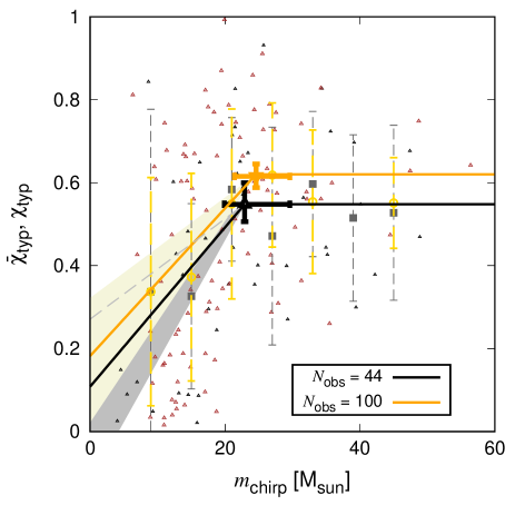
Figure 6.— The ${\bar{\chi}}_{\rm typ}$ profile as a function of $m_{\mathrm{chirp}}$ constructed using the mock GW data for $100$ (orange), and $44$ (black) observed events. Thick lines present the recovered profiles as in Fig. 5. The triangles corresponds to the median values of ${\chi}_{\rm typ}$ for all mock events. The dashed lines show $1\sigma$ credible intervals for observed values of ${\bar{\chi}}_{\rm typ}$ for mock events.

3.3. Reconstruction of the spin profile from mock GW data

We investigate how well the ${\bar{\chi}}_{\mathrm{typ}}$ profile can be reconstructed from mock GW data ($\S\,\ref{sec:mock_data}$) for different values of $N_{\mathrm{obs}}$ by performing the MCMC method as described in $\S\,\ref{sec:method_reconstruction_spin}$. Fig. 6 shows ${\bar{\chi}}_{\mathrm{typ}}$ as a function of $m_{\mathrm{chirp}}$ for $N_{\mathrm{obs}}=44$ (black) and $N_{\mathrm{obs}}=100$ (orange) for the model with the fiducial setting (Table 1) but $m_{\mathrm{max}}=30\,{\rm M}_{\odot}$ and $\alpha=2$, which is preferred from observed GW events ($\S\,\ref{sec:result_rec_x_obs}$ and $\S\,\ref{sec:results_bayesian_factor}$).

As the parameter estimate tends to be biased in small $N_{\mathrm{obs}}$, we additionally perform 10 models for $N_{\mathrm{obs}}=44$ with same settings with independent realizations of the initial condition. By averaging the estimated parameters for eleven models, ${\bar{\chi}}_{\mathrm{typ}}$ at the plateau is $b_{\mu}=0.63^{+0.07}_{-0.05}$ with the standard deviation $\sigma(b_{\mu})=0.04$, the critical chirp mass is $m_{\mathrm{crit}}=24^{+6}_{-4}\,{\rm M}_{\odot}$ with $\sigma(m_{\mathrm{crit}})=5\,{\rm M}_{\odot}$, and the slope of ${\bar{\chi}}_{\mathrm{typ}}$ in $m_{\mathrm{chirp}}<m_{\mathrm{crit}}$ is $a_{\mu}=25^{+9}_{-8}\times 10^{-3}\,{\rm M}_{\odot}^{-1}$ with $\sigma(b_{\mu})=8\times 10^{-3}\,{\rm M}_{\odot}^{-1}$. As these uncertainties on the reconstructed parameters from the GW mock data are similar to those derived from the observed GW data in $\S\,\ref{sec:result_rec_x_obs}$, we conclude that the GW mock data are a useful tool to understand how well the spin profile can be reconstructed.

The critical chirp mass is estimated to be $m_{\mathrm{crit}}=25^{+6}_{-3}\,{\rm M}_{\odot}$ for $N_{\mathrm{obs}}=100$, and $m_{\mathrm{crit}}=24.9^{+0.9}_{-0.8}\,{\rm M}_{\odot}$ for $N_{\mathrm{obs}}=1000$. Here, the estimated value of $m_{\mathrm{crit}}$ is lower than $m_{\mathrm{max}}$ by $\sim 20\%$ mostly because $m_{\mathrm{chirp}}=(m_{\mathrm{1}}+m_{\mathrm{2}})[q(1+q)^{-2}]^{3/5}\lesssim 0.87m_{\mathrm{max}}$. As the analysis on the observed GW events in $\S\,\ref{sec:result_rec_x_obs}$ derives $m_{\mathrm{crit}}\sim 15$–$50\,{\rm M}_{\odot}$, $m_{\mathrm{max}}\sim 20$–$60\,{\rm M}_{\odot}$ is roughly inferred according to the relation of $m_{\mathrm{max}}\sim 1.2\,m_{\mathrm{crit}}$.

The average spin parameter ${\bar{\chi}}_{\mathrm{typ}}$ at $m_{\mathrm{chirp}}=m_{\mathrm{min}}$ is related to the typical spin magnitude of 1g BHs (e.g. Fig. 1). ${\bar{\chi}}_{\mathrm{typ}}$ at $m_{\mathrm{chirp}}=5\,{\rm M}_{\odot}$ is $0.20^{+0.14}_{-0.17}$ for $N_{\mathrm{obs}}=44$, $0.27^{+0.11}_{-0.13}$ for $N_{\mathrm{obs}}=100$, and $0.23^{+0.03}_{-0.02}$ for $N_{\mathrm{obs}}=1000$. These values derived from the model with $a_{\mathrm{ave}}=a_{\mathrm{uni}}=0$ are similar to the value ($\sim 0.3\pm\sim 0.1$) derived from the observed GW data ($\S\,\ref{sec:result_rec_x_obs}$), suggesting that the typical spin magnitude of 1g BHs inferred from the observed GW events is still consistent with $\sim 0$.

For $N_{\mathrm{obs}}=100$, ${\bar{\chi}}_{\mathrm{typ}}$ at the plateau is $b_{\mu}=0.62^{+0.04}_{-0.03}$, which is similar to the expected value for hierarchical mergers ($\sim 0.6$, $\S\,\ref{sec:result_pop_parameters}$). Also, the mass at the bending point is well constrained with $N_{\mathrm{obs}}=100$ as mentioned above. Thus, with $N_{\mathrm{obs}}\geq 100$, parameters characterising properties of hierarchical mergers, e.g. a value of ${\bar{\chi}}_{\mathrm{typ}}$ and $m_{\mathrm{crit}}$ at the plateau, are more precisely constrained.

Finally, to investigate whether the bending point is robustly verified, we also fit the distribution by a straight line, i.e. assuming $m_{\mathrm{crit}}\rightarrow\infty$ in Eq. (16), and calculate the Bayes factor of the model with broken lines (Eq. 16) compared to the model with a single line ($m_{\mathrm{crit}}\rightarrow\infty$), where we set the likelihood function to Eq. (16) with the fitted parameters. For $N_{\mathrm{obs}}=44$, 100, and 1000, the logarithm of the Bayes factor is 1.5, 2.1, and 24, respectively. If we adopt the Akaike information criterion (Akaike, 1974), the model with the broken lines is preferred by a factor of $\sim 10^{1.6}$ for $N_{\mathrm{obs}}=100$, and the preference increases as $N_{\mathrm{obs}}$ increases. In the analysis using the observed data in $\S$ 3.2.1, although we assumed the existence of the plateau, the Bayes factors using the observed events (with $D_{\mathrm{KL,cri}}=0$, 0.05, 0.1, and $0.15$) are in the range of $10^{-0.2}$–$10^{0.2}$, suggesting that the existence of the plateau is uncertain. Our analysis suggests that as the number of GW events increases to $\gtrsim O(100)$, the existence of the plateau can be confirmed with high significance.

4. Summary and Conclusions

In this paper we have investigated characteristic distributions of $\chi_{\mathrm{eff}}$, $\chi_{\mathrm{p}}$, $\chi_{\mathrm{typ}}=(\chi_{\mathrm{p}}^{2}+\chi_{\mathrm{eff}}^{2})^{1/2}$, and $m_{\mathrm{chirp}}$ expected from hierarchical mergers among stellar-mass BHs. We then used a toy model to derive the profile of the average of $\chi_{\mathrm{typ}}$ as a function of $m_{\mathrm{chirp}}$ for the events observed by LIGO/Virgo O1–O3a. We also investigated how well predictions in different models match observed spin and mass distributions by using Bayes factors. Finally, we estimate how well the $\chi_{\mathrm{typ}}$ profile can be reconstructed using mock GW data expected in hierarchical mergers. Our main results are summarized as follows:

1. If hierarchical mergers are frequent, and the spin distribution of first-generation (1g) BHs does not strongly depend on their mass, the ${\bar{\chi}}_{\mathrm{typ}}$ profile as a function of $m_{\mathrm{chirp}}$ is characterized by a monotonic increase of ${\bar{\chi}}_{\mathrm{typ}}$ with $m_{\mathrm{chirp}}$ up to the maximum chirp mass among 1g BHs, and reaches a plateau of ${\bar{\chi}}_{\mathrm{typ}}$ with $\sim 0.6$ at higher $m_{\mathrm{chirp}}$ (Fig. 1). With $\sim 50$ events, the plateau and the rise of $\chi_{\mathrm{typ}}$ to $0.6$ can be confirmed if the detection fraction of mergers of high-g BHs roughly exceeds $\sim 0.5$ and $\sim 0.15$, respectively.

2. The maximum mass for 1g BHs can be estimated by constraining the transition point between the two regimes in the ${\bar{\chi}}_{\mathrm{typ}}$ profile. Also, the typical spin magnitude for 1g BHs is constrained from ${\bar{\chi}}_{\mathrm{typ}}$ at around minimum $m_{\mathrm{chirp}}$ among GW events.

3. The ${\bar{\chi}}_{\mathrm{typ}}$ profile reconstructed from the LIGO/Virgo O1–O3a data prefers an increase in ${\bar{\chi}}_{\mathrm{typ}}$ at $m_{\mathrm{chirp}}\lesssim 15$–$50\,{\rm M}_{\odot}$ with $\sim 2\sigma$ confidence (Fig. 5), consistent with the evolution of BH spin magnitudes by hierarchical mergers. The maximum mass and the typical spin magnitude of 1g BHs are loosely constrained to be $\sim 20$–$60\,{\rm M}_{\odot}$ and $\lesssim 0.4$ with $\sim 1\sigma$ credible intervals, respectively.

4. A Bayesian analysis using the $\chi_{\mathrm{eff}}$, $\chi_{\mathrm{p}}$, and $m_{\mathrm{chirp}}$ distributions suggests that 1g BHs are preferred to have the maximum mass of $m_{\mathrm{max}}\sim 15$–$30\,{\rm M}_{\odot}$ if hierarchical mergers are frequent, which is consistent with mergers in AGN disks and/or nuclear star clusters. On the other hand, if mergers mainly originate from globular clusters (in which $m_{\mathrm{max}}$ is assumed to be $45\,{\rm M}_{\odot}$), 1g BHs are favored to have spin magnitudes of $\sim 0.3$. These favored models are also consistent with the average and the standard deviation of $\chi_{\mathrm{p}}$ estimated in The LIGO Scientific Collaboration et al. (2020c).

5. By using observed data of more than $\sim 100$ events in the future, we will be able to recover parameters characterizing the ${\bar{\chi}}_{\mathrm{typ}}$ distribution (e.g. the existence of the plateau and the value of ${\bar{\chi}}_{\mathrm{typ}}$ at the plateau $b_{\mu}$) more precisely.

DATA AVAILABILITY

The data underlying this article will be shared on reasonable request to the corresponding author.

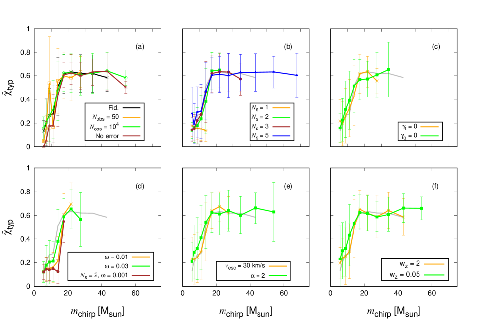
Figure 7.— Same as Fig. 1, but present for models M1, M14–M28 (Table 2). We use $N_{\mathrm{obs}}=10^{3}$ detectable mergers for models M1, M14–M28, while $N_{\mathrm{obs}}=50$ and $10^{4}$ for models M14 and M15, respectively.

Table 5 Same as Table 2, but includes models M14–M28.

model	Parameter	high-g fraction	high-g detection fraction	$m_{\mathrm{chirp,max}}[{\rm M}_{\odot}]$	${\bar{\chi}}_{\mathrm{p}}$	$\sigma(\chi_{\mathrm{p}})$
M1	Fiducial	0.33	0.68	56	0.17	0.26
M2	Globular cluster (GC)	0.063	0.17	44	0.030	0.13
M3	Field binary (FB)	0	0	23	0	0
M4	Migration trap (MT)	0.31	0.80	42	0	0
M5	$a_{\mathrm{uni}}=1$	0.32	0.73	52	0.50	0.21
M6	$a_{\mathrm{ave}}=0.99$	0.31	0.70	51	0.75	0.20
M7	$a_{\mathrm{ave}}=0.66$, $a_{\mathrm{uni}}=0.1$	0.33	0.72	55	0.55	0.13
M8	$a_{\mathrm{ave}}=0.5$	0.33	0.74	65	0.46	0.12
M9	$m_{\mathrm{max}}=30\,{\rm M}_{\odot}$	0.35	0.73	70	0.18	0.26
M10	$N_{\mathrm{obs}}=50$, $N_{\mathrm{s}}=3$	0.25	0.62	28	0.13	0.24
M11	$N_{\mathrm{obs}}=50$, $N_{\mathrm{s}}=2$	0.15	0.28	24	0.077	0.19
M12	$N_{\mathrm{obs}}=50$, $N_{\mathrm{s}}=2$, $\omega=0.05$	0.077	0.18	19	0.040	0.14
M13	$N_{\mathrm{obs}}=50$, $N_{\mathrm{s}}=2$, $\omega=0.03$	0.046	0.14	19	0.023	0.11
M14	$N_{\mathrm{obs}}=50$	0.33	0.78	38	0.17	0.26
M15	$N_{\mathrm{obs}}=10^{4}$	0.33	0.77	60	0.17	0.26
M16	$N_{\mathrm{s}}=1$	0	0	15	0	0
M17	$N_{\mathrm{s}}=2$	0.15	0.40	23	0.077	0.19
M18	$N_{\mathrm{s}}=3$	0.25	0.61	42	0.13	0.24
M19	$N_{\mathrm{s}}=5$	0.38	0.80	72	0.20	0.27
M20	$\gamma_{\mathrm{t}}=0$	0.22	0.50	31	0.11	0.22
M21	$\gamma_{\mathrm{q}}=0$	0.39	0.71	36	0.19	0.25
M22	$\omega=0.01$	0.043	0.089	23	0.022	0.11
M23	$\omega=0.03$	0.13	0.37	33	0.066	0.18
M24	$N_{\mathrm{s}}=2$, $\omega=0.001$	0.0014	0.0040	17	0.001	0.02
M25	$v_{\mathrm{esc}}=30\,\mathrm{km/s}$	0.29	0.61	31	0.15	0.25
M26	$\alpha=2$	0.32	0.75	52	0.16	0.25
M27	$w_{\mathrm{z}}=2$	0.33	0.73	46	0.17	0.26
M28	$w_{\mathrm{z}}=0.05$	0.33	0.79	59	0.17	0.26

Appendix A Dependence on population parameters

We show the parameter dependence of the ${\bar{\chi}}_{\mathrm{typ}}$ profile as a function of $m_{\mathrm{chirp}}$ using mock GW events, in which hierarchical mergers are assumed to be frequent. In Table 5, we list the model varieties we have investigated (models M1–M28). We additionally examine different choices of the number of detected mergers (models M14 and M15), the steps to create samples for hierarchical mergers (models M16–M19), pairing probability (models M20 and M21), the fraction of mergers in each step (models M22–M24), the escape velocity of the system (model M25), the power law for mass function (model M26), and the correlation between the steps and the redshift (models M27 and M28).

With smaller number of iteration steps ($N_{\mathrm{s}}$), the maximum $m_{\mathrm{chirp}}$ becomes smaller because the generations of BHs are limited by $N_{\mathrm{s}}$ (panel b of Fig. 7). Similarly, the maximum $m_{\mathrm{chirp}}$ decreases as $N_{\mathrm{obs}}$, $\gamma_{\mathrm{t}}$, $\omega$, or $v_{\mathrm{esc}}$ decreases or $m_{\mathrm{max}}$ increases (panels a, c, d, and e of Fig. 7 and panel b of Fig. 1, Table 5). In these ways, the maximum $m_{\mathrm{chirp}}$ is influenced by a number of parameters, implying that the maximum $m_{\mathrm{chirp}}$ alone cannot constrain each of those parameters.

Here, we investigate the effect that mergers at larger iteration steps tend to occur at lower redshift because finite time needs to elapse between each generation and high-g mergers thus would take place after a significant delay compared to low-g mergers. To take this delay into account, we modify the redshift distribution of merging BHs as

$$p_{z}\propto \frac{dV_{c}}{dz}\frac{1}{1+z}\mathrm{exp}\left(\frac{(t_{\mathrm{L}}(z)-\mu_{t})^{2}}{2\sigma_{t}^{2}}\right),$$ (A1)

where $t_{\mathrm{L}}(z)$ is the look-back time, we set the average to $\mu_{t}=t_{\mathrm{typ}}\left(\frac{N_{\mathrm{s}}-N_{i}+1}{N_{\mathrm{s}}}\right)$ and the standard deviation to $\sigma_{t}=t_{\mathrm{typ}}w_{t}$, $N_{i}$ is the number of steps that the $i^{\mathrm{th}}$ merger is created, $t_{\mathrm{typ}}$ is the typical look-back time that mergers began to occur, which is set to $10\,\mathrm{Gyr}$, and $w_{z}$ is the parameter determining the strength of correlation between $N_{i}$ and the time that mergers occur. A lower value of $w_{z}$ makes mergers with high $N_{i}$ occur at a lower $z$, and the fiducial model (Eq. 7) corresponds to $w_{z}=\infty$. The dependence of the ${\bar{\chi}}_{\mathrm{typ}}$ profile on $w_{z}$ is shown in panel (f), suggesting that the correlation between the redshift and the generations of BHs has a negligible impact on the profile.

Appendix B Observed spin distribution

We presents the observed distributions of $\chi_{\mathrm{p}}$, $\chi_{\mathrm{eff}}$, and $\chi_{\mathrm{typ}}$ as a function of $m_{\mathrm{chirp}}$ in Fig. 8. Also, Fig. 9 compares the $m_{\mathrm{chirp}}$, $\chi_{\mathrm{eff}}$ and $\chi_{\mathrm{p}}$ distributions observed by LIGO/Virgo O1–O3a and those predicted by the model for the fiducial settings (Table 1) but $m_{\mathrm{max}}=30\,{\rm M}_{\odot}$ and $\alpha=2$, which is assessed to high Bayes factors for both $D_{\mathrm{KL,crit}}=0.05$ and the two parameters (Table 4). We can see that the observed distribution for these variables (blue and orange points) roughly follows the 90 and 99 percentile regions (black and gray lines) predicted by the model.

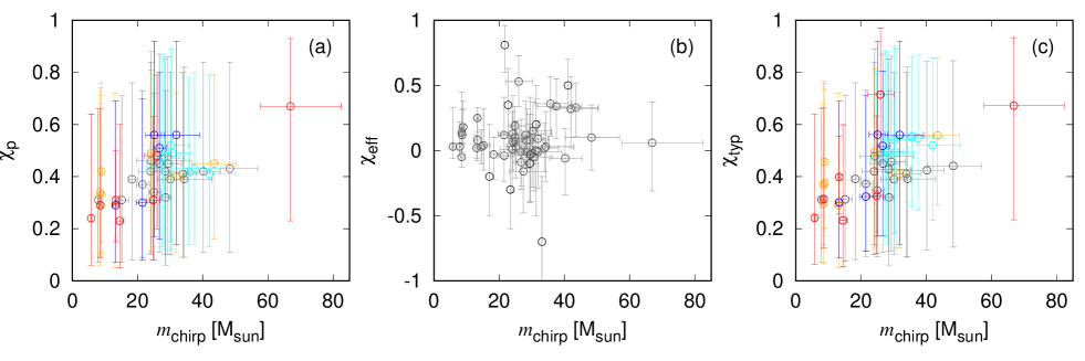
Figure 8.— Observed distribution for spins reported in LIGO/Virgo O1–O3a. Panels (a)–(c) represent the distributions of $\chi_{\mathrm{p}}$, $\chi_{\mathrm{eff}}$, and $\chi_{\mathrm{typ}}$, respectively. Red, blue, orange, cyan, and gray circles represent events with the KL divergence between prior and posterior samples for $\chi_{\mathrm{p}}$ to be $D_{\mathrm{KL}}\geq 0.2$, $0.2>D_{\mathrm{KL}}\geq 0.15$, $0.15>D_{\mathrm{KL}}\geq 0.1$, $0.1>D_{\mathrm{KL}}\geq 0.05$, and $0.05>D_{\mathrm{KL}}$, respectively. Bars correspond to the $90$ percentile credible intervals.

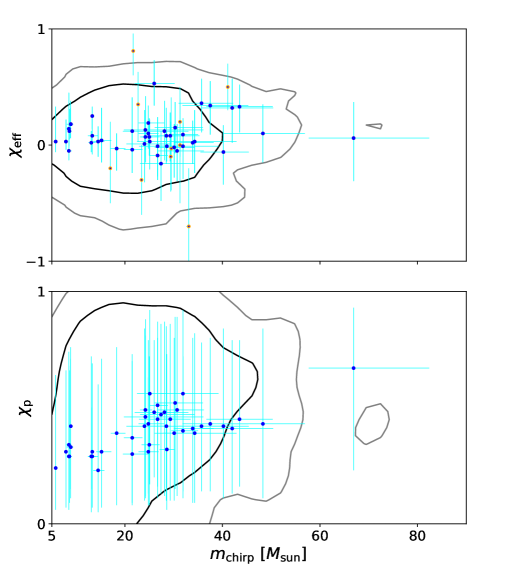
Figure 9.— Comparisons between the $\chi_{\mathrm{eff}}$ (upper) or $\chi_{\mathrm{p}}$ (lower) and $m_{\mathrm{chirp}}$ distributions observed by LIGO/Virgo O1–O3a and those predicted by the model with $m_{\mathrm{max}}=30\,{\rm M}_{\odot}$ and $\alpha=2$ which have high Bayes factors (Table 4). Black and gray lines correspond to 90 and 99 credible intervals for the predicted distributions, and cyan bars correspond to the 90 percentile credible intervals for the observed variables. The orange points in the upper panel corresponds to the events reported in Venumadhav et al. (2019) and Zackay et al. (2019).

Appendix C Posterior distributions for spin parameters

We present the posterior distributions of the parameters characterizing the spin profile for the GW events with $D_{\rm KL}\geq 0$ ($\S\,\ref{sec:result_rec_x_obs}$) in Fig. 10.

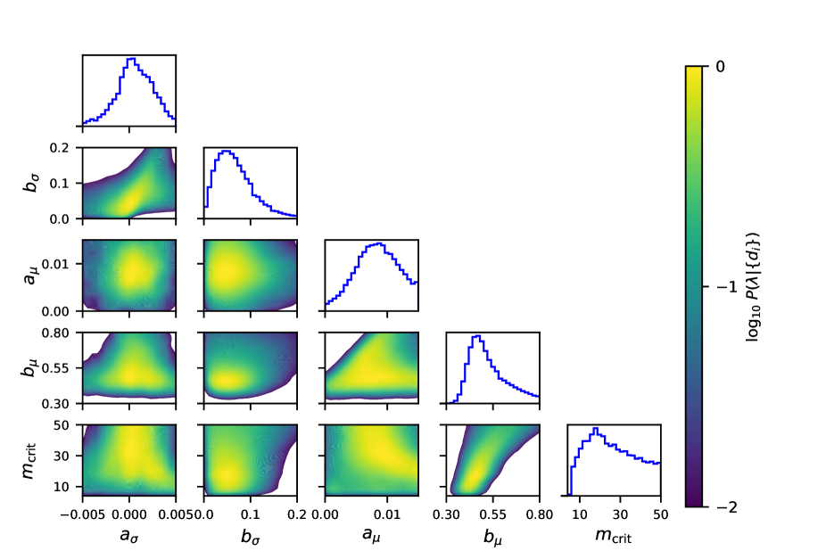
Figure 10.— The posterior probability distributions for $a_{\sigma}$, $b_{\sigma}$, $a_{\mu}$, $b_{\mu}$, and $m_{\rm crit}$ for $D_{\rm KL,crit}=0$ ($\S\,\ref{sec:result_rec_x_obs}$).

References

- Aasi et al. (2015) Aasi, J., et al. 2015, CQG, 32, 074001
- Abbott et al. (2019) Abbott, B. P., Abbott, R., Abbott, T. D., et al. 2019, Physical Review X, 9, 031040
- Abbott et al. (2020a) Abbott, R., Abbott, T. D., Abraham, S., et al. 2020a, ApJ, 896, L44
- Abbott et al. (2020b) —. 2020b, arXiv e-prints, arXiv:2010.14527
- Abbott et al. (2020c) —. 2020c, ApJ, 900, L13
- Acernese et al. (2015) Acernese, F., et al. 2015, CQG, 32, 024001
- Akaike (1974) Akaike, H. 1974, IEEE Transactions on Automatic Control, 19, 716
- Antonini et al. (2019) Antonini, F., Gieles, M., & Gualandris, A. 2019, MNRAS, 486, 5008
- Antonini et al. (2017) Antonini, F., Toonen, S., & Hamers, A. S. 2017, ApJ, 841, 77
- Apostolatos et al. (1994) Apostolatos, T. A., Cutler, C., Sussman, G. J., & Thorne, K. S. 1994, Phys. Rev. D, 49, 6274
- Arca Sedda (2020) Arca Sedda, M. 2020, arXiv e-prints, arXiv:2002.04037
- Askar et al. (2020) Askar, A., Davies, M. B., & Church, R. P. 2020, arXiv e-prints, arXiv:2006.04922
- Banerjee (2017) Banerjee, S. 2017, MNRAS, 467, 524
- Bardeen & Petterson (1975) Bardeen, J. M., & Petterson, J. A. 1975, ApJ, 195, L65
- Bartos et al. (2017) Bartos, I., Kocsis, B., Haiman, Z., & Márka, S. 2017, ApJ, 835, 165
- Bavera et al. (2019) Bavera, S. S., Fragos, T., Qin, Y., et al. 2019, arXiv e-prints, arXiv:1906.12257
- Belczynski et al. (2016) Belczynski, K., Daniel, E. H., Bulik, T., & O’Shaughnessy, R. 2016, Nature, 534, 512
- Bellovary et al. (2016) Bellovary, J. M., Mac Low, M.-M., McKernan, B., & Ford, K. E. S. 2016, ApJ, 819, L17
- Brodie et al. (2014) Brodie, J. P., Romanowsky, A. J., Strader, J., et al. 2014, ApJ, 796, 52
- Buonanno et al. (2008) Buonanno, A., Kidder, L. E., & Lehner, L. 2008, Phys. Rev. D, 77, 026004
- Chatzopoulos & Wheeler (2012) Chatzopoulos, E., & Wheeler, J. C. 2012, ApJ, 748, 42
- Chen et al. (2017) Chen, H.-Y., Holz, D. E., Miller, J., et al. 2017, arXiv e-prints, arXiv:1709.08079
- de Mink & Mandel (2016) de Mink, S. E., & Mandel, I. 2016, MNRAS, 460, 3545
- Di Carlo et al. (2019) Di Carlo, U. N., Giacobbo, N., Mapelli, M., et al. 2019, MNRAS, 487, 2947
- Do et al. (2018) Do, T., Kerzendorf, W., Konopacky, Q., et al. 2018, ApJ, 855, L5
- Doctor et al. (2020) Doctor, Z., Wysocki, D., O’Shaughnessy, R., Holz, D. E., & Farr, B. 2020, ApJ, 893, 35
- Dominik et al. (2012) Dominik, M., Belczynski, K., Fryer, C., et al. 2012, ApJ, 759, 52
- Farmer et al. (2019) Farmer, R., Renzo, M., de Mink, S. E., Marchant, P., & Justham, S. 2019, ApJ, 887, 53
- Fishbach & Holz (2020) Fishbach, M., & Holz, D. E. 2020, ApJ, 891, L27
- Fishbach et al. (2017) Fishbach, M., Holz, D. E., & Farr, B. 2017, ApJ, 840, L24
- Fishbach et al. (2018) Fishbach, M., Holz, D. E., & Farr, W. M. 2018, ApJ, 863, L41
- Fragione et al. (2019) Fragione, G., Grishin, E., Leigh, N. W. C., Perets, H. B., & Perna, R. 2019, MNRAS, 488, 47
- Fragione & Kocsis (2018) Fragione, G., & Kocsis, B. 2018, Phys. Rev. Lett., 121, 161103
- Fragione & Kocsis (2019) —. 2019, MNRAS, 486, 4781
- Fragione et al. (2020) Fragione, G., Loeb, A., & Rasio, F. A. 2020, ApJ, 902, L26
- Fuller & Ma (2019) Fuller, J., & Ma, L. 2019, ApJ, 881, L1
- Gerosa & Berti (2017) Gerosa, D., & Berti, E. 2017, Phys. Rev. D, 95, 124046
- Gerosa et al. (2019) Gerosa, D., Lima, A., Berti, E., et al. 2019, Classical and Quantum Gravity, 36, 105003
- Gerosa et al. (2020a) Gerosa, D., Mould, M., Gangardt, D., et al. 2020a, arXiv e-prints, arXiv:2011.11948
- Gerosa et al. (2020b) Gerosa, D., Vitale, S., & Berti, E. 2020b, arXiv e-prints, arXiv:2005.04243
- Gondán et al. (2018) Gondán, L., Kocsis, B., Raffai, P., & Frei, Z. 2018, ApJ, 860, 5
- Hamers & Safarzadeh (2020) Hamers, A. S., & Safarzadeh, M. 2020, ApJ, 898, 99
- Hannam et al. (2014) Hannam, M., Schmidt, P., Bohé, A., et al. 2014, Phys. Rev. Lett., 113, 151101
- Hastings (1970) Hastings, W. K. 1970, Biometrika, 57, 97
- Hotokezaka & Piran (2017) Hotokezaka, K., & Piran, T. 2017, ApJ, 842, 111
- Inayoshi et al. (2017) Inayoshi, K., Hirai, R., Kinugawa, T., & Hotokezaka, K. 2017, MNRAS, 468, 5020
- Ivanova et al. (2013) Ivanova, N., Justham, S., Chen, X., et al. 2013, The Astronomy and Astrophysics Review, 21, 59
- Kalogera (2000) Kalogera, V. 2000, ApJ, 541, 319
- Kesden et al. (2010) Kesden, M., Sperhake, U., & Berti, E. 2010, Phys. Rev. D, 81, 084054
- Kidder (1995) Kidder, L. E. 1995, Phys. Rev. D, 52, 821
- Kimball et al. (2020a) Kimball, C., Talbot, C., Berry, C. P. L., et al. 2020a, ApJ, 900, 177
- Kimball et al. (2020b) —. 2020b, arXiv e-prints, arXiv:2011.05332
- Kinugawa et al. (2014) Kinugawa, T., Inayoshi, K., Hotokezaka, K., Nakauchi, D., & T., N. 2014, MNRAS, 442, 2963
- Kocsis et al. (2011) Kocsis, B., Yunes, N., & Loeb, A. 2011, Phys. Rev. D, 84, 024032
- Kumamoto et al. (2018) Kumamoto, J., Fujii, M. S., & Tanikawa, A. 2018, arXiv e-prints, arXiv:1811.06726
- Leaman et al. (2013) Leaman, R., VandenBerg, D. A., & Mendel, J. T. 2013, MNRAS, 436, 122
- LIGO Scientific Collaboration & Virgo Collaboration (2020) LIGO Scientific Collaboration, & Virgo Collaboration. 2020, LIGO Document P1800370-v5 https://dcc.ligo.org/LIGO-P1800370/public
- LIGO Scientific Collaboration & Virgo Collaboration (2021) —. 2021, LIGO Document P2000223-v7, https://dcc.ligo.org/LIGO-P2000223/public/
- Liu & Lai (2020) Liu, B., & Lai, D. 2020, arXiv e-prints, arXiv:2009.10068
- Lubow et al. (1999) Lubow, S. H., Seibert, M., & Artymowicz, P. 1999, ApJ, 526, 1001
- Mandel & de Mink (2016) Mandel, I., & de Mink, S. E. 2016, MNRAS, 458, 2634
- Mandel et al. (2019) Mandel, I., Farr, W. M., & Gair, J. R. 2019, MNRAS, 486, 1086
- Mapelli et al. (2020) Mapelli, M., Santoliquido, F., Bouffanais, Y., et al. 2020, arXiv e-prints, arXiv:2007.15022
- Marchant et al. (2016) Marchant, P., Langer, N., Podsiadlowski, P., Tauris, T., & Moriya, T. 2016, A&A, 588, A50
- McKernan et al. (2020a) McKernan, B., Ford, K. E. S., & O’Shaughnessy, R. 2020a, MNRAS, 498, 4088
- McKernan et al. (2020b) McKernan, B., Ford, K. E. S., O’Shaugnessy, R., & Wysocki, D. 2020b, MNRAS, 494, 1203
- McKernan et al. (2018) McKernan, B., Ford, K. E. S., Bellovary, J., et al. 2018, ApJ, 866, 66
- Michaely & Perets (2019) Michaely, E., & Perets, H. B. 2019, ApJ, 887, L36
- Moody et al. (2019) Moody, M. S. L., Shi, J.-M., & Stone, J. M. 2019, arXiv e-prints, arXiv:1903.00008
- O’Leary et al. (2009) O’Leary, R. M., Kocsis, B., & Loeb, A. 2009, MNRAS, 395, 2127
- O’Leary et al. (2016) O’Leary, R. M., Meiron, Y., & Kocsis, B. 2016, ApJL, 824, L12
- Olejak et al. (2020) Olejak, A., Fishbach, M., Belczynski, K., et al. 2020, ApJ, 901, L39
- Paczynski (1976) Paczynski, B. 1976, in IAU Symposium, Structure and Evolution of Close Binary Systems, 73, 75
- Pan & Yang (2021) Pan, Z., & Yang, H. 2021, arXiv e-prints, arXiv:2101.09146
- Pavlovskii et al. (2017) Pavlovskii, K., Ivanova, N., Belczynski, K., & Van, K. X. 2017, MNRAS, 465, 2092
- Peng et al. (2006) Peng, E. W., Jordán, A., Côté, P., et al. 2006, ApJ, 639, 95
- Planck Collaboration et al. (2016) Planck Collaboration, Ade, P. A. R., Aghanim, N., et al. 2016, A&A, 594, A13
- Portegies Zwart & McMillan (2000) Portegies Zwart, S. F., & McMillan, S. L. W. 2000, ApJ, 528, L17
- Pratten et al. (2020) Pratten, G., Schmidt, P., Buscicchio, R., & Thomas, L. M. 2020, Physical Review Research, 2, 043096
- Rasskazov & Kocsis (2019) Rasskazov, A., & Kocsis, B. 2019, arXiv e-prints, arXiv:1902.03242
- Rastello et al. (2019) Rastello, S., Amaro-Seoane, P., Arca-Sedda, M., et al. 2019, MNRAS, 483, 1233
- Rastello et al. (2020) Rastello, S., Mapelli, M., Di Carlo, U. N., et al. 2020, MNRAS, 497, 1563
- Rodriguez et al. (2018) Rodriguez, C. L., Amaro-Seoane, P., Chatterjee, S., & Rasio, F. A. 2018, Phys. Rev. Lett., 120, 151101
- Rodriguez et al. (2016a) Rodriguez, C. L., Chatterjee, S., & Rasio, F. A. 2016a, Phys. Rev. D., 93, 084029
- Rodriguez et al. (2019) Rodriguez, C. L., Zevin, M., Amaro-Seoane, P., et al. 2019, Phys. Rev. D, 100, 043027
- Rodriguez et al. (2016b) Rodriguez, C. L., Zevin, M., Pankow, C., Kalogera, V., & Rasio, F. A. 2016b, ApJ, 832, L2
- Rodriguez et al. (2020) Rodriguez, C. L., Kremer, K., Grudić, M. Y., et al. 2020, ApJ, 896, L10
- Safarzadeh et al. (2020a) Safarzadeh, M., Farr, W. M., & Ramirez-Ruiz, E. 2020a, arXiv e-prints, arXiv:2001.06490
- Safarzadeh & Haiman (2020) Safarzadeh, M., & Haiman, Z. 2020, arXiv e-prints, arXiv:2009.09320
- Safarzadeh et al. (2020b) Safarzadeh, M., Hamers, A. S., Loeb, A., & Berger, E. 2020b, ApJ, 888, L3
- Samsing et al. (2014) Samsing, J., MacLeod, M., & Ramirez-Ruiz, E. 2014, ApJ, 784, 71
- Samsing et al. (2020) Samsing, J., Bartos, I., D’Orazio, D. J., et al. 2020, arXiv e-prints, arXiv:2010.09765
- Schmidt et al. (2015) Schmidt, P., Ohme, F., & Hannam, M. 2015, Phys. Rev. D, 91, 024043
- Schödel et al. (2020) Schödel, R., Nogueras-Lara, F., Gallego-Cano, E., et al. 2020, arXiv e-prints, arXiv:2007.15950
- Scott (1992) Scott, D. 1992, Multivariate Density Estimation: Theory, Practice, and Visualization, A Wiley-interscience publication (Wiley)
- Silsbee & Tremaine (2017) Silsbee, K., & Tremaine, S. 2017, ApJ, 836, 39
- Spera et al. (2019) Spera, M., Mapelli, M., Giacobbo, N., et al. 2019, MNRAS, 485, 889
- Stone et al. (2017) Stone, N. C., Metzger, B. D., & Haiman, Z. 2017, MNRAS, 464, 946
- Tagawa et al. (2020a) Tagawa, H., Haiman, Z., Bartos, I., & Kocsis, B. 2020a, ApJ, 899, 26
- Tagawa et al. (2020b) Tagawa, H., Haiman, Z., & Kocsis, B. 2020b, ApJ, 898, 25
- Tagawa et al. (2021a) Tagawa, H., Kocsis, B., Haiman, Z., et al. 2021a, ApJ, 907, L20
- Tagawa et al. (2021b) —. 2021b, ApJ, 908, 194
- Tagawa et al. (2018) Tagawa, H., Kocsis, B., & Saitoh, R. T. 2018, Phys. Rev. Lett., 120, 261101
- The LIGO Scientific Collaboration et al. (2019) The LIGO Scientific Collaboration, the Virgo Collaboration, Abbott, B. P., et al. 2019, arXiv e-prints, arXiv:1906.08000
- The LIGO Scientific Collaboration et al. (2020a) The LIGO Scientific Collaboration, the Virgo Collaboration, Abbott, R., et al. 2020a, arXiv e-prints, arXiv:2004.08342
- The LIGO Scientific Collaboration et al. (2020b) —. 2020b, arXiv e-prints, arXiv:2009.01075
- The LIGO Scientific Collaboration et al. (2020c) —. 2020c, arXiv e-prints, arXiv:2010.14533
- Tiwari & Fairhurst (2020) Tiwari, V., & Fairhurst, S. 2020, arXiv e-prints, arXiv:2011.04502
- van den Heuvel et al. (2017) van den Heuvel, E. P. J., Portegies Zwart, S. F., & de Mink, S. E. 2017, MNRAS, 471, 4256
- Veitch et al. (2015) Veitch, J., Raymond, V., Farr, B., et al. 2015, Phys. Rev. D, 91, 042003
- Venumadhav et al. (2019) Venumadhav, T., Zackay, B., Roulet, J., Dai, L., & Zaldarriaga, M. 2019, arXiv e-prints, arXiv:1904.07214
- Vink et al. (2021) Vink, J. S., Higgins, E. R., Sander, A. A. C., & Sabhahit, G. N. 2021, MNRAS, 504, 146
- Vitale et al. (2020) Vitale, S., Gerosa, D., Farr, W. M., & Taylor, S. R. 2020, arXiv e-prints, arXiv:2007.05579
- Yang et al. (2020a) Yang, Y., Bartos, I., Haiman, Z., et al. 2020a, arXiv e-prints, arXiv:2003.08564
- Yang et al. (2020b) Yang, Y., Gayathri, V., Bartos, I., et al. 2020b, arXiv e-prints, arXiv:2007.04781
- Yang et al. (2019) Yang, Y., Bartos, I., Gayathri, V., et al. 2019, Phys. Rev. Lett., 123, 181101
- Yoon et al. (2012) Yoon, S. C., Dierks, A., & Langer, N. 2012, A&A, 542, A113
- Zackay et al. (2019) Zackay, B., Dai, L., Venumadhav, T., Roulet, J., & Zaldarriaga, M. 2019, arXiv e-prints, arXiv:1910.09528
- Zevin et al. (2020a) Zevin, M., Spera, M., Berry, C. P. L., & Kalogera, V. 2020a, ApJ, 899, L1
- Zevin et al. (2020b) Zevin, M., Bavera, S. S., Berry, C. P. L., et al. 2020b, arXiv e-prints, arXiv:2011.10057
- Ziosi et al. (2014) Ziosi, B. M., Mapelli, M., Branchesi, M., & Tormen, G. 2014, MNRAS, 441, 3703