Faithful analytical effective one body waveform model for spin-aligned, moderately eccentric, coalescing black hole binaries

Abstract

We present a new effective-one-body (EOB) model for eccentric binary coalescences. The model stems from the state-of-the-art model TEOBiResumS_SM for circularized coalescing black-hole binaries, that is modified to explicitly incorporate eccentricity effects both in the radiation reaction and in the waveform. Using Regge-Wheeler-Zerilli type calculations of the gravitational wave losses as benchmarks, we find that a rather accurate ($\sim 1\%$) expression for the radiation reaction along mildly eccentric orbits ($e\sim 0.3$) is given by dressing the current, EOB-resummed, circularized angular momentum flux, with a leading-order (Newtonian-like) prefactor valid along general orbits. An analogous approach is implemented for the waveform multipoles. The model is then completed by the usual merger-ringdown part informed by circularized numerical relativity (NR) simulations. The model is validated against the 22, publicly available, NR simulations calculated by the Simulating eXtreme Spacetime (SXS) collaboration, with mild eccentricities, mass ratios between 1 and 3 and up to rather large dimensionless spin values ($\pm 0.7$). The maximum EOB/NR unfaithfulness, calculated with Advanced LIGO noise, is at most of order $3\%$. The analytical framework presented here should be seen as a promising starting point for developing highly-faithful waveform templates driven by eccentric dynamics for present, and possibly future, gravitational wave detectors.

I Introduction

Parameter estimates of all gravitational wave (GW) signals from coalescing binaries are done under the assumption that the inspiral is quasi-circular Abbott et al. (2019). This is motivated by the efficient circularization of the inspiral due to gravitational wave emission. In addition, no explicit evidence for eccentricity for some events was found Abbott et al. (2017); Nitz et al. (2019); Romero-Shaw et al. (2020). However, recent population synthesis studies Samsing et al. (2014); Rodriguez et al. (2016); Belczynski et al. (2016); Samsing (2018) suggest that active galactic nuclei and globular clusters may host a population of eccentric binaries. Currently, there are no ready-to-use waveform models that accurately combine both eccentricity and spin effects over the entire parameter space. Recently, numerical relativity (NR) started producing surveys of eccentric, spinning binary black hole (BBH) coalescence waveforms Hinder et al. (2017); Ramos-Buades et al. (2019); Huerta et al. (2019), and a NR-surrogate waveform model for nonspinning eccentric binaries up to mass ratio $q=10$ exists Huerta et al. (2019). On the analytical side, Refs. Klein et al. (2018); Tiwari et al. (2019) provided closed-form eccentric inspiral templates (based on the Quasi-Keplerian approximation). Similarly, a few exploratory effective-one-body (EOB)-based Buonanno and Damour (1999, 2000); Buonanno et al. (2006); Damour et al. (2015) studies were recently performed Cao and Han (2017); Hinderer and Babak (2017); Liu et al. (2019). In particular Refs. Cao and Han (2017); Liu et al. (2019) introduced and tested SEOBNRE, a way to incorporate eccentricity within the SEOBNRv1 Taracchini et al. (2012) circularized waveform model. However, the SEOBNRv1 model is outdated now, since it does not accurately cover high-spins, nor mass ratios up to 10. This drawback is inherited by the SEOBNRE model Liu et al. (2019).

In this article, we modify a highly NR-faithful EOB multipolar waveform model for circularized coalescing BBHs, TEOBiResumS_SM Nagar et al. (2018, 2020), to incorporate eccentricity-dependent effects. The EOB formalism relies on three building blocks: (i) a Hamiltonian, that describes the conservative part of the relative dynamics; (ii) a radiation reaction force, that accounts for the back-reaction onto the system due to the GW losses of energy and angular momentum; (iii) a prescription for computing the waveform. Including eccentricity requires modifications to blocks (ii) and (iii) with respect to the quasi-circular case.

II Radiation reaction and waveform for eccentric inspirals

Within the EOB formalism, we use phase-space variables $(r,\varphi,p_{\varphi},p_{r_{*}})$, related to the physical ones by $r=R/(GM)$ (relative separation), $p_{r_{*}}=P_{R_{*}}/\mu$ (radial momentum), $p_{\varphi}=P_{\varphi}/(\mu GM)$ (angular momentum) and $t=T/(GM)$ (time), where $\mu\equiv m_{1}m_{2}/M$ and $M=m_{1}+m_{2}$. The radial momentum is $p_{r_{*}}\equiv(A/B)^{1/2}p_{r}$, where $A$ and $B$ are the EOB potentials. The EOB Hamiltonian is $\hat{H}_{\rm EOB}\equiv H_{\rm EOB}/\mu=\nu^{-1}\sqrt{1+2\nu(\hat{H}_{\rm eff}-1)}$, with $\nu\equiv\mu/M$ and $\hat{H}_{\rm eff}=\tilde{G}p_{\varphi}+\hat{H}^{\rm orb}_{\rm eff}$, where $\tilde{G}p_{\varphi}$ incorporates odd-in-spin (spin-orbit) effects while $\hat{H}^{\rm orb}_{\rm eff}$ incorporates even-in-spin effects Nagar et al. (2018). We denote dimensionless spin variables as $\chi_{i}\equiv S_{i}/m_{i}^{2}$. The TEOBiResumS_SM Nagar and Shah (2016); Messina et al. (2018); Nagar et al. (2020) waveform model is currently the most NR faithful model versus the zero_det_highP Advanced LIGO design sensitivity Shoemaker ). Reference Nagar et al. (2020) found that the maximum value of the EOB/NR unfaithfulness is always below $0.5\%$ all over the current release of the SXS NR waveform catalog Chu et al. (2009); Lovelace et al. (2011, 2012); Buchman et al. (2012); Hemberger et al. (2013); Scheel et al. (2015); Blackman et al. (2015); Lovelace et al. (2015); Mroue et al. (2013); Kumar et al. (2015); Chu et al. (2016); Boyle et al. (2019); SXS . This is achieved by NR informing a 4.5PN spin-orbit effective function $c_{3}(\nu,\chi_{1},\chi_{2})$ and an effective 5PN function $a_{6}^{c}(\nu)$ entering the Padé resummed radial potential $A(r)$. [see Eqs. (39) and (33) of Ref. Nagar et al. (2019a)]. The two Hamilton’s equations that take account of GW losses are

$$\dot{p}_{\varphi} =\hat{{\cal F}}_{\varphi},$$ (1)

$$\dot{p}_{r_{*}} =\sqrt{\frac{A}{B}}\left(-\partial_{r}\hat{H}_{\rm EOB}+\hat{{\cal F}}_{r}\right),$$ (2)

where $(\hat{{\cal F}}_{\varphi},\hat{{\cal F}}_{r})$ are the two radiation reaction forces. In the quasi-circular case Nagar et al. (2018); Ossokine et al. one sets $\hat{{\cal F}}_{r}=0$. Here, we use $\hat{{\cal F}}_{r}\neq 0$ and $\hat{{\cal F}}_{\varphi}$ explicitly includes noncircular terms. The main technical issue is to build (resummed) expressions of $(\hat{{\cal F}}_{\varphi},\hat{{\cal F}}_{r})$ that are reliable and robust up to merger. Building upon Ref. Gopakumar et al. (1997), Ref. Bini and Damour (2012) derived the 2PN-accurate, generic expressions of $(\hat{{\cal F}}_{\varphi},\hat{{\cal F}}_{r})$, which are unsuited to drive the transition from the EOB inspiral to plunge and merger: they are nonresummed and generally unreliable in the strong-field regime (see below). The forces are related to the instantaneous losses of energy and angular momentum through GWs. Following Ref. Bini and Damour (2012), there exists a gauge choice such that the balance equations read

$$-\dot{J}^{\infty} ={\cal F}_{\varphi},$$ (3)

$$-\dot{E}^{\infty} =\dot{r}{\cal F}_{r}+\dot{\varphi}{\cal F}_{\varphi}+\dot{E}_{\rm Schott},$$ (4)

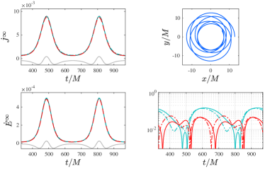
Figure 1: Test-particle orbiting a Schwarzschild black hole with semilatus rectum $p=9$ and eccentricity $e=0.3$. Different analytical representations of the angular momentum and energy fluxes $(\dot{J}^{\infty},\dot{E}^{\infty})$ are compared with the numerical ones using the Regge-Wheeler-Zerilli (RWZ) formalism (black). Left panels: the nonresummed 2PN-accurate ones of Ref. Bini and Damour (2012), (gray); the resummed version via Eq. (5) (light-blue); the resummed version using the noncircular Newtonian prefactor (red), Eq. (8). The relative differences in $(\dot{J}^{\infty},\dot{E}^{\infty})$ are shown in the bottom-right panel: $|\delta\dot{J}^{\infty}/\dot{J}_{\rm RWZ}^{\infty}|$ (solid) and $|\delta\dot{E}^{\infty}/\dot{E}_{\rm RWZ}^{\infty}|$ (dashed), color scheme as above. On average, Eq. (8) delivers the closest analytical/numerical agreement.

where $E_{\rm Schott}$ is the Schott energy (see Ref. Damour et al. (2012); Bini and Damour (2012) and references therein), $(\dot{E},\dot{J})^{\infty}$ are the energy and angular momentum fluxes at infinity, while ${\cal F}_{\varphi,r}\equiv\mu\hat{{\cal F}}_{\varphi,r}$. To build the resummed expressions of the functions $({\cal F}_{\varphi},{\cal F}_{r},\dot{E}_{\rm Schott})$ and evaluate their strong-field reliability, we adopt the procedure that proved fruitful in the circularized case Damour et al. (1998, 2009); Pan et al. (2011); Nagar and Shah (2016); Messina et al. (2018); Nagar et al. (2019b): any analytical choice for $({\cal F}_{\varphi},{\cal F}_{r},\dot{E}_{\rm Schott})$ is tested by comparisons with the energy and angular momentum fluxes emitted by a test particle orbiting a Schwarzschild black hole on eccentric orbits. We focus first on ${\cal F}_{\varphi}$. We start with the 2PN-accurate result of Ref. Bini and Damour (2012) [see Eq. (3.70) and Appendix D therein], ${\cal F}_{\varphi}^{\rm 2PN}(r,p_{r},p_{\varphi})$, reexpress it in terms of $p_{r_{*}}$, and factor it in a circular part (defined imposing $p_{r_{*}}=\dot{p}_{r_{*}}=0$), ${\cal F}^{\rm 2PN_{c}}_{\varphi}(r)$, and a noncircular contribution, ${\cal F}^{\rm 2PN_{\rm nc}}_{\varphi}(r,p_{r_{*}},p_{\varphi})$, so that ${\cal F}^{\rm 2PN}_{\varphi}(r,p_{r_{*}},p_{\varphi})={\cal F}^{\rm 2PN_{c}}_{\varphi}(r){\cal F}^{\rm 2PN_{\rm nc}}_{\varphi}(r,p_{r_{*}},p_{\varphi})$. A route to improve the strong-field behavior of this expression is to replace ${\cal F}^{\rm 2PN_{c}}_{\varphi}(r)$ with the corresponding EOB-resummed expression Damour et al. (2009) (notably, in its latest avatar Nagar et al. (2020); Nagar and Shah (2016); Messina et al. (2018)). To do so, the radial EOB coordinate $r$ in ${\cal F}^{\rm 2PN_{c}}_{\varphi}(r)$ is first replaced by the circularized frequency variable $x\equiv\Omega_{\rm circ}^{2/3}$, Eq. (5.22) of Ref. Bini and Damour (2012) at 2PN accuracy; then this 2PN-accurate expression is replaced by ${\cal F}_{\varphi}^{\rm EOB_{c}}(x)=-32/5\nu^{2}x^{7/2}\hat{f}(x)$, where $\hat{f}\equiv\left(F_{22}^{\rm Newt}\right)^{-1}\sum_{\ell m}F_{{\ell m}}$ is the factored flux function Damour et al. (2009), with all multipoles (except $m=0$ ones) up to $\ell=8$. Finally, the function ${\cal F}_{\varphi}^{\rm EOB_{c}}(x)$ is computed along the noncircular dynamics. We do so by using the circular frequency $\Omega_{\rm circ}\equiv\partial_{p_{\varphi}}\hat{H}_{\rm EOB}|_{p_{\varphi}=j,p_{r_{*}}=0}$, where $j^{2}\equiv-A^{\prime}(u)/(u^{2}A(u))^{\prime}$ is the (squared) circular angular momentum, $u\equiv r^{-1}$ and $(\cdot)^{\prime}\equiv\partial_{u}$. Note that in the resummed flux, we use $\{p_{\varphi},\hat{H}_{\rm EOB}(r,p_{r_{*}},p_{\varphi}),\hat{H}_{\rm eff}(r,p_{r_{*}},p_{\varphi})\}$ computed along the general dynamics. The 2PN-accurate noncircular contribution ${\cal F}^{\rm 2PN_{nc}}_{\varphi}\equiv f_{\varphi}^{N_{\rm nc}}+c^{-2}f_{\varphi}^{\rm 1PN_{nc}}+c^{-4}f_{\varphi}^{\rm 2PN_{\rm nc}}$ is resummed using a $(0,2)$ Padé approximant. We have

$${\cal F}_{\varphi}^{\rm EOB_{2PN_{nc}}}\equiv{\cal F}_{\varphi}^{\rm EOB_{c}}(x(r))P^{0}_{2}[{\cal F}_{\varphi}^{\rm 2PN_{nc}}(r,p_{r_{*}},p_{\varphi})].$$ (5)

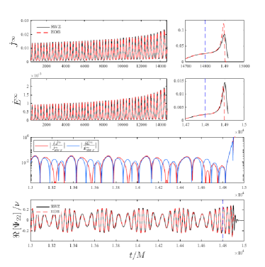
Figure 2: Test particle (with mass ratio $\mu/M=10^{-3}$, $e=0.3)$ and $p=8$) plunging over a Schwarzschild black hole. EOB/RWZ comparison between energy and angular momentum fluxes (top three panels) and waveforms (bottom panel). Vertical line: crossing of the stability threshold ($p=6+2e$) and beginning of the plunge.

Alternatively, we recall that the force used to drive the EOB quasi-circular inspiral is

$${\cal F}_{\varphi}^{\rm EOB_{qc}}=-\dfrac{32}{5}\nu^{2}r_{\omega}^{4}\Omega^{5}\hat{f}(\Omega),$$ (6)

where $\Omega\equiv\dot{\varphi}$, which yields a more faithful representation of GW losses during the plunge Damour and Gopakumar (2006); Damour and Nagar (2007). This expression is the leading quasi-circular term of the Newtonian angular momentum flux, obtained from Eq. (3.26) of Ref. Bini and Damour (2012), neglecting higher-order derivatives of $(r,\Omega)$. We can thus improve Eq. (6) multiplying it with the Newtonian noncircular factor

$$\hat{f}_{\varphi}^{\rm{Newt}_{nc}}=1+\dfrac{3}{4}\dfrac{\ddot{r}^{2}}{r^{2}\Omega^{4}}-\dfrac{\ddot{\Omega}}{4\Omega^{3}}+\dfrac{3\dot{r}\dot{\Omega}}{r\Omega^{3}}$$ (7)

$$+\dfrac{4\dot{r}^{2}}{r^{2}\Omega^{2}}+\dfrac{\ddot{\Omega}\dot{r}^{2}}{8r^{2}\Omega^{5}}+\dfrac{3}{4}\dfrac{\dot{r}^{3}\dot{\Omega}}{r^{3}\Omega^{5}}+\dfrac{3}{4}\dfrac{\dot{r}^{4}}{r^{4}\Omega^{4}}+\dfrac{3}{4}\dfrac{\dot{\Omega}^{2}}{\Omega^{4}}$$

$$-\dddot{r}\left(\dfrac{\dot{r}}{2r^{2}\Omega^{4}}+\dfrac{\dot{\Omega}}{8r\Omega^{5}}\right)+\ddot{r}\left(-\dfrac{2}{r\Omega^{2}}+\dfrac{\ddot{\Omega}}{8r\Omega^{5}}+\dfrac{3}{8}\dfrac{\dot{r}\dot{\Omega}}{r^{2}\Omega^{5}}\right),$$

in order to get

$${\cal F}_{\varphi}^{\rm EOB_{Newt_{nc}}}=-\dfrac{32}{5}\nu^{2}r_{\omega}^{4}\Omega^{5}\hat{f}_{\varphi}^{\rm{Newt}_{nc}}\hat{f}(\Omega).$$ (8)

Although this expression incorporates formally less noncircular PN information than Eq. (5), the time-derivatives (and $\hat{f}(\Omega)$ as well) are obtained from the full EOB (resummed) equations of motion rather the 2PN ones used in ${\cal F}_{\varphi}^{\rm 2PN_{nc}}$. For ${\cal F}_{r}$, we build on Ref. Bini and Damour (2012) and we use ${\cal F}_{r}=32/3p_{r_{*}}/r^{4}P^{0}_{2}[\hat{{\cal F}}^{\rm 2PN}_{r}]$, where $P^{0}_{2}$ is the $(0,2)$ Padé approximant and $\hat{\cal F}^{\rm 2PN}_{r}=f_{r}^{N}+c^{-2}f_{r}^{\rm 1PN}+c^{-4}f_{r}^{\rm 2PN}$ is the 2PN accurate expression calculated from Eqs. (3.70) and (D9-D11) of Ref. Bini and Damour (2012). We adopt an analogous approach to deal with the Schott energy, as given by Eqs. (3.57) and (C1-C4) of Ref. Bini and Damour (2012). We factorize it in circular and noncircular parts that are both resummed with the $P^{0}_{2}$ Padé approximant, so to have $E_{\rm Schott}=16/5p_{r_{*}}/r^{3}P^{0}_{2}[E_{\rm Schott}^{\rm c}]P^{0}_{2}[E_{\rm Schott}^{\rm nc}]$, where $E_{\rm Schott}^{\rm nc}=E^{\rm nc,0}_{\rm Schott}+c^{-2}E^{\rm nc,1PN}_{\rm Schott}+c^{-4}E^{\rm nc,2PN}_{\rm Schott}$.

Table 1: SXS simulations with eccentricity analyzed in this work. From left to right: the ID of the simulation; the mass ratio $q\equiv m_{1}/m_{2}\geq 1$; the individual spins $(\chi_{1},\chi_{2})$; the estimated NR eccentricity at first apastron $e_{\rm\omega}^{\rm NR}$; the initial EOB eccentricity $e^{\rm EOB}$ and apastron frequency $\omega_{a}^{\rm EOB}$ which allow us to get a good EOB/NR frequency agreement.

SXS	$q$	$\chi_{1}$	$\chi_{2}$	$e^{\rm NR}_{\rm\omega}$	$e^{\rm EOB}$	$\omega_{a}^{\rm EOB}$	$\max(\bar{F})[\%]$
1355	1	0	0	0.062	0.089	0.0280475	1.30
1356	1	0	0	0.102	0.1503	0.019077	1.03
1359	1	0	0	0.112	0.18	0.021495	1.22
1357	1	0	0	0.114	0.1916	0.019617	1.20
1361	1	0	0	0.160	0.23437	0.02104	1.56
1360	1	0	0	0.161	0.2415	0.019635	1.52
1362	1	0	0	0.217	0.30041	0.0192	0.89
1364	2	0	0	0.049	0.0843	0.025241	0.86
1365	2	0	0	0.067	0.11	0.023987	1.00
1367	2	0	0	0.105	0.1494	0.026078	0.92
1369	2	0	0	0.201	0.309	0.01755	1.38
1371	3	0	0	0.063	0.0913	0.029058	0.57
1372	3	0	0	0.107	0.149	0.026070	0.95
1374	3	0	0	0.208	0.31405	0.016946	0.78
89	1	$-0.5$	0	0.047	0.071	0.0178279	0.96
1136	1	$-0.75$	$-0.75$	0.078	0.121	0.02728	0.58
321	1.22	$+0.33$	$-0.44$	0.048	0.076	0.02694	1.47
322	1.22	$+0.33$	$-0.44$	0.063	0.0984	0.026895	1.18
323	1.22	$+0.33$	$-0.44$	0.104	0.141	0.025965	1.57
324	1.22	$+0.33$	$-0.44$	0.205	0.2915	0.019067	2.25
1149	3	$+0.70$	$+0.60$	0.037	$0.0617$	$0.0266802$	3.16
1169	3	$-0.70$	$-0.60$	0.036	$0.049$	$0.024285$	0.17

Equations (5)-(8) are specialized to the test particle limit ($\nu=0$) and computed along the eccentric, conservative, dynamics of a particle orbiting a Schwarzschild black hole. The result is compared with the fluxes computed using Regge-Wheeler-Zerilli (RWZ) black hole perturbation theory Regge and Wheeler (1957); Zerilli (1970); Nagar and Rezzolla (2005). To accurately extract waves at future null infinity, we adopt the hyperboloidal layer method of Bernuzzi et al. (2011) and compute the fluxes with the usual expressions of Ref. Nagar and Rezzolla (2005), including all multipoles up to $\ell=8$. Figure 1 shows the illustrative case of an orbit with semilatus rectum $p=9$ and eccentricity $e=0.3$. The apastron is $r_{1}=p/(1-e)$, and the periastron is $r_{2}=p/(1+e)$ . The figure indicates that ${\cal F}_{\varphi}^{\rm EOB_{Newt_{nc}}}$ delivers analytical energy and angular momentum fluxes (red lines) that are, on average, in better agreement with the RWZ ones than those obtained from ${\cal F}_{\varphi}^{\rm EOB_{2PN_{nc}}}$, which increase up to a $10\%$ fractional difference at apastron. We adopt then ${\cal F}_{\varphi}^{\rm EOB_{Newt_{nc}}}$ as analytical representation of the angular momentum flux along generic orbits. The maximal analytical/RWZ flux relative differences are $\sim 10^{-2}$. The robustness of this result is checked by considering several orbits with $p$ varying from just above the stability threshold ($p=6+2e$) up to $p=21$, and for each $p$ we consider $0\leq e\leq 0.9$. We then compute the relative flux differences $(\delta\dot{E},\delta\dot{J})$ at periastron for each $(p,e)$. We find that, for each value of $p$, $(\delta\dot{E},\delta\dot{J})$ are at most of the order of $10\%$ for $e=0.9$. More interestingly if $e\lesssim 0.3$, the fractional differences do not exceed the $5\%$ level.

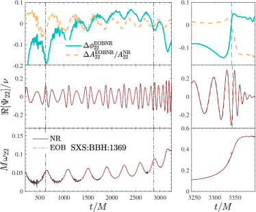
Figure 3: Illustrative EOB/NR time-domain waveform comparison for the nonspinning configuration SXS:BBH:1369, with $e_{\omega}^{\rm NR}=0.201$, $q=2$ and $\chi_{1}=\chi_{2}=0$.

Let us consider now the waveform emitted from the transition from inspiral to plunge, merger and ringdown as driven by $({\cal F}_{r},{\cal F}_{\varphi}^{\rm EOB_{Newt_{nc}}})$, focusing on a test-particle (of mass ratio $\mu/M=10^{-3}$) on a Schwarzschild background. To efficiently compute, along the relative dynamics, up to the third time-derivative of the phase-space variables entering Eq. (7), we suitably generalize the iterative analytical procedure used in Appendix A of Ref. Damour et al. (2013) to calculate $\ddot{r}$. We checked that two iterations are sufficient to obtain an excellent approximation $(\simeq 10^{-3})$ of the derivatives computed numerically. An illustrative waveform is displayed in Fig. 2 for $p=8$ and $e=0.3$ (initial values). The top three rows of the figure highlight the numerical consistency ($\sim 10^{-2}$) between the RWZ angular momentum and energy fluxes and their analytical counterparts. The corresponding waveform is shown (in black) in the fourth row of the plot. The gravitational waveform is decomposed in multipoles as $h_{+}-{\rm i}h_{\times}=D_{L}^{-1}\sum_{\ell m}h_{\ell m}{}_{-2}Y_{{\ell m}}$, where $D_{L}$ is the luminosity distance and ${}_{-2}Y_{{\ell m}}$ the $s=-2$ spin-weighted spherical harmonics. We use below the RWZ normalized variable $\Psi_{{\ell m}}=h_{{\ell m}}/\sqrt{(\ell+2)(\ell+1)\ell(\ell-1)}$.

Figure 4: EOB/NR unfaithfulness computed over the eccentric SXS simulations publicly available. The horizontal lines mark the $3\%$ and $1\%$ values.

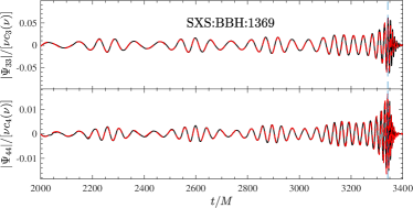
Figure 5: Illustrative EOB/NR comparison for SXS:BBH:1369 for the $(3,3)$ and $(4,4)$ waveform modes. Normalization constants are $c_{3}=\sqrt{1-4\nu}$ and $c_{4}=1-3\nu$.

A detailed analysis of the properties of the RWZ waveform, such as the excitation of QNMs, etc., will be presented elsewhere. Here we employ it as a target, an “exact” waveform to validate the EOB one. Within the EOB formalism, each multipole is factorized as $h_{{\ell m}}=h_{\ell m}^{(N,\epsilon)}\hat{h}_{\ell m}$, where $h_{\ell m}^{(N,\epsilon)}$ is the Newtonian (leading-order) prefactor, $\hat{h}_{\ell m}$ is the resummed relativistic correction Damour et al. (2009) and $\epsilon$ the parity of $\ell+m$. The circularized prefactor $h_{\ell m}^{(N,\epsilon)}$ is replaced by its general expression obtained computing the time-derivatives of the Newtonian mass and current multipoles. We have $h_{\ell m}^{(N,0)}\propto e^{{\rm i}m\varphi}I^{(\ell)}_{\ell m}$ and $h_{\ell m}^{(N,1)}\propto e^{{\rm i}m\varphi}S^{(\ell)}_{\ell m}$, where $(\ell)$ indicates the $\ell$-th time-derivative and $I_{\ell m}\equiv r^{\ell}e^{-{\rm i}m\varphi}$ and $S_{\ell m}\equiv r^{\ell+1}\Omega e^{-{\rm i}m\varphi}$ are the Newtonian mass and current multipoles. The $\ell=m=2$ mode of the analytical waveform is superposed, as a red line, in the bottom row of Fig. 2, showing excellent agreement with the RWZ one essentially up to merger. A similar agreement is found for subdominant modes.

III Comparison with numerical relativity simulations

The complete, $\nu$-dependent, radiation reaction of above replaces now the standard one used in TEOBiResumS_SM, so to consistently drive an eccentric inspiral. Everything is analogous to the test-particle case, aside from (i) the initial conditions at the apastron, which are more involved because of the presence of spin, though they are a straightforward generalization of those of Hinderer and Babak (2017); (ii) similar complications for the time-derivatives needed in $\hat{f}^{{\rm Newt}_{\rm nc}}$. The EOB waveform with the noncircular Newtonian prefactors is completed by next-to-quasi-circular (NQC) corrections and the NR-informed circularized ringdown Nagar et al. (2018, 2020). Differently from the circularized case, the NQC correction factor is smoothly activated in time just when getting very close to merger, so to avoid spurious contaminations during the inspiral. Also, no iteration on the NQC amplitude parameters is performed Nagar et al. (2020). We assess the quality of the analytic waveforms by comparing them with the sample of eccentric NR simulations publicly available in the SXS catalog Chu et al. (2009); Lovelace et al. (2011, 2012); Buchman et al. (2012); Hemberger et al. (2013); Scheel et al. (2015); Blackman et al. (2015); Lovelace et al. (2015); Mroue et al. (2013); Kumar et al. (2015); Chu et al. (2016); Boyle et al. (2019); SXS that are listed in Table 1. We carry out both time-domain comparisons and compute the EOB/NR unfaithfulness. To do so correctly the EOB evolution should be started in such a way that the eccentricity-induced frequency oscillations are consistent with the corresponding ones in the NR simulations. Since the eccentricities are gauge dependent, their nominal values are meaningless for this purpose. EOB and NR waveforms are then aligned in the time-domain Damour et al. (2013) during the early inspiral and then we progressively vary the initial GW frequency at apastron, $\omega_{a}^{\rm EOB}$, and eccentricity, $e^{\rm EOB}$, until we achieve minimal fractional differences ($\simeq 10^{-2}$) between the EOB and NR GW frequencies. To facilitate the parameter choice, we also estimate the initial (at first apastron) eccentricity of each NR simulation, $e_{\omega}^{\rm NR}$, using the method proposed in Eq. (2.8) of Ref. Ramos-Buades et al. (2019), where $e_{\omega}$ is deduced from the frequency oscillations; we here employ, however, the frequency of the $(2,2)$ mode, as opposed to the orbital frequency as done in Ref. Ramos-Buades et al. (2019). The last two columns of Table 1 contain the values of $(\omega_{a}^{\rm EOB},e^{\rm EOB})$ that lead to the best agreement between NR and EOB waveforms. An illustrative time-domain comparison, for SXS:BBH:1369 is shown in Fig. 3. Figure 4 shows the EOB/NR unfaithfulness $\bar{F}\equiv 1-F$ (see Eq. (48) of Ref. Nagar et al. (2020)) computed with the zero_det_highP Shoemaker Advanced-LIGO power spectral density. Both NR and EOB waveforms (starting at approximately the same frequency) were suitably tapered in the early inspiral. From Table 1, $\max(\bar{F})$ is always comfortably below $3\%$ except for the, small-eccentricity, dataset SXS:BBH:1149, with $\max(\bar{F})=3.16$. We believe that this is the effect of the suboptimal choice of $(a_{6}^{c},c_{3})$ (see below) and is not related to the modelization of eccentricity effects. By contrast, for large eccentricities, the $\bar{F}$ computation may be influenced by the accuracy of NR simulations, which get progressively more noisy increasing $e_{\omega}$ (see e.g. bottom panel of Fig. 3; a similar behavior is also found for SXS:BBH:324). The accumulated phase difference at meger (always $\sim 1$ rad) is mostly due to the previously determined Nagar et al. (2020) $(a_{6}^{c},c_{3})$ values, that depend on the circularized waveform and radiation reaction. Consistently, when our generalized framework is applied to circularized (nonspinning) binaries, we find that $\max(\bar{F})$ varies between $1.25\%$ ($q=1$) and $0.21\%$ ($q=8$). These values are about one order of magnitude larger than those of TEOBiResumS_SM(see Fig. 13 of Nagar et al. (2019a)). Forthcoming work will present a retuning of $(a_{6}^{c},c_{3})$ so to improve the EOB/NR agreement further. Some subdominant multipoles are rather robust in the nonspinning case, see e.g. Fig. 5. For large spins, we find the same problems related to the correct determination of NQC corrections found for TEOBiResumS_SM Nagar et al. (2020). Highly-accurate NR simulations covering a larger portion of the parameter space (see e.g. Ref. Ramos-Buades et al. (2019)) are thus needed to robustly validate the model when $e_{\omega}^{\rm NR}\gtrsim 0.2$.

IV Conclusions

We illustrated that minimal modifications to TEOBiResumS_SM Nagar et al. (2020) enabled us to build a (mildly) eccentric waveform model that is reasonably NR-faithful over a nonnegligible portion of the parameter space. This model could provide new eccentricity measurements on LIGO-Virgo events. Our approach can be applied also in the presence of tidal effects. Higher-order corrections in the waveforms and flux (see Refs. Mishra et al. (2015); Cao and Han (2017); Hinderer and Babak (2017)) should be included to improve the model for larger eccentricities. In this respect, with a straighforward modification of the initial conditions Damour et al. (2014), our model can also generate waveforms for dynamical captures or hyperbolic encounters East et al. (2013), although NR validation is needed Gold and Brügmann (2013); Damour et al. (2014). Provided high-order, gravitational-self-force informed, resummed expressions for the EOB potentials Akcay et al. (2012); Bini and Damour (2014); Akcay and van de Meent (2016); Antonelli et al. (2020); Barack et al. (2019), as well as analytically improved fluxes to enhance the analytical/numerical agreement of Fig. 1 for larger eccentricities, we believe that our approach can pave the way to the efficient construction of EOB-based waveform templates for extreme mass ratio inspirals, as interesting sources for LISA Babak et al. (2015); Berry et al. (2019).