The Black Hole Accretion Code

Abstract

We present the black hole accretion code (BHAC), a new multidimensional general-relativistic magnetohydrodynamics module for the MPI-AMRVAC framework . BHAC has been designed to solve the equations of ideal general-relativistic magnetohydrodynamics in arbitrary spacetimes and exploits adaptive mesh refinement techniques with an efficient block-based approach. Several spacetimes have already been implemented and tested. We demonstrate the validity of BHAC by means of various one-, two-, and three-dimensional test problems, as well as through a close comparison with the HARM3D code in the case of a torus accreting onto a black hole. The convergence of a turbulent accretion scenario is investigated with several diagnostics and we find accretion rates and horizon-penetrating fluxes to be convergent to within a few percent when the problem is run in three dimensions. Our analysis also involves the study of the corresponding thermal synchrotron emission, which is performed by means of a new general-relativistic radiative transfer code, BHOSS​​. The resulting synthetic intensity maps of accretion onto black holes are found to be convergent with increasing resolution and are anticipated to play a crucial role in the interpretation of horizon-scale images resulting from upcoming radio observations of the source at the Galactic Center.

Research

1 Introduction

Accreting black holes (BHs) are amongst the most powerful astrophysical objects in the Universe. A substantial fraction of the gravitational binding energy of the accreting gas is released within tens of gravitational radii from the BH, and this energy supplies the power for a rich phenomenology of astrophysical systems including active galactic nuclei, X-ray binaries and gamma-ray bursts. Since the radiated energy originates from the vicinity of the BH, a fully general-relativistic treatment is essential for the modelling of these objects and the flows of plasma in their vicinity.

Depending on the mass accretion rate, a given system can be found in various spectral states, with different radiation mechanisms dominating and varying degrees of coupling between radiation and gas (Fender2004, ; Markoff2005, ). Some supermassive BHs, including the primary targets of observations by the Event-Horizon-Telescope Collaboration (EHTC), i.e., Sgr A* and M87, are accreting well below the Eddington accretion rate Marrone2007 ; Ho2009 . In this regime, the accretion flow advects most of the viscously released energy into the BH rather than radiating it to infinity. Such optically thin, radiatively inefficient and geometrically thick flows are termed advection-dominated accretion flows (ADAFs, see Narayan1994 ; Narayan1995 ; Abramowicz1995 ; Yuan2014 ) and can be modelled without radiation feedback. Next to the ADAF, two additional radiatively inefficient accretion flows (RIAFs) exist: The advection-dominated inflow-outflow solution (ADIOS) Blandford1999 ; Begelman2012 and the convection-dominated accretion flow (CDAF) Narayan2000 ; Quataert2000 , which include respectively, the physical effects of outflows and convection. Analytical and semi-analytical approaches are reasonably successful in reproducing the main features in the spectra of ADAFs (see, e.g.,  Yuan2003, ). However, numerical general-relativistic magnetohydrodynamic (GRMHD) simulations are essential to gain an understanding of the detailed physical processes at play in the Galactic Centre and other low-luminosity compact objects.

Modern BH accretion-disk theory suggests that angular momentum transport is due to MHD turbulence driven by the magnetorotational instability (MRI) within a differentially rotating disk (Balbus1991, ; BalbusHawley1998, ). Recent non-radiative GRMHD simulations of BH accretion systems in an ADAF regime have resolved these processes and reveal a flow structure that can be decomposed into a disk, a corona, a disk-wind and a highly magnetized polar funnel (see, e.g.,  DeVilliers03, ; McKinney2004, ; McKinney2006c, ; McKinney2009, ). The simulations show complex time-dependent behaviour in the disk, corona and wind. Depending on BH spin, the polar regions of the flow contain a nearly force-free, Poynting–flux-dominated jet (see, e.g.,  Blandford1977, ; McKinney2004, ; Hawley2006, ; McKinney2006c, ).

In addition to having to deal with highly nonlinear dynamics that spans a large range in plasma parameters, the numerical simulations also need to follow phenomena that occur across multiple physical scales. For example, in the MHD paradigm, jet acceleration is an intrinsically inefficient process that requires a few thousand gravitational radii to reach equipartition of the energy fluxes Komissarov2007b ; Barkov2008 (purely hydrodynamical mechanisms can however be far more efficient Aloy:2006rd ). Jet-environment interactions like the prominent HST-1 feature of the radio-galaxy M87 Biretta1989 ; Stawarz2006 ; Asada2012 occur on scales of $\sim 5\times 10^{5}$ gravitational radii. Hence, for a self-consistent picture of accretion and ejection, jet formation and recollimation due to interaction with the environment (see, e.g.,  Mizuno2015, ), numerical simulations must capture horizon-scale processes, as well as parsec-scale interactions with an overall spatial dynamic range of $\sim 10^{5}$. The computational cost of such large-scale grid-based simulations quickly becomes prohibitive. Adaptive mesh refinement (AMR) techniques promise an effective solution for problems where it is necessary to resolve small and large scale dynamics simultaneously.

Another challenging scenario is presented by radiatively efficient geometrically thin accretion disks that mandate extreme resolution in the equatorial plane in order to resolve the growth of MRI instabilities. Typically this is dealt with by means of stretched grids that concentrate resolution where needed (Avara2016, ; Sadowski2016a, ). However, when the disk is additionally tilted with respect to the spin axis of the BH (Fragile2007b, ; McKinney2013, ), lack of symmetry forbids such an approach. Here an adaptive mesh that follows the warping dynamics of the disk can be of great value. The list of scenarios where AMR can have transformative qualities due to the lack of symmetries goes on, the modelling of star-disk interactions Giannios2013 , star-jet interactions BarkovAharonian2010 , tidal disruption events (Tchekhovskoy2014, ), complex shock geometries Nagakura2008 ; Meliani2017 , and intermittency in driven-turbulence phenomena Radice2012b ; Zrake2013 , will benefit greatly from adaptive mesh refinement.

Over the past few years, the development of general-relativistic numerical codes employing the $3+1$ decomposition of spacetime and conservative “Godunov” schemes based on approximate Riemann solvers Rezzolla_book:2013 ; Font03 ; Marti2015 have led to great advances in numerical relativity. Many general-relativistic hydrodynamic (HD) and MHD codes have been developed (Hawley84a, ; Koide00, ; DeVilliers03a, ; Gammie03, ; Baiotti04, ; Duez05MHD0, ; Anninos05c, ; Anton05, ; Mizuno06, ; DelZanna2007, ; Giacomazzo:2007ti, ; Radice2012a, ; Radice2013b, ; McKinney2014, ; Etienne2015, ; White2015, ; Zanotti2015, ; Meliani2017, ) and applied to study a variety of problems in high-energy astrophysics. Some of these implementations provide additional capabilities that incorporate approximate radiation transfer (see, e.g.,  Sadowski2013, ; McKinney2013b, ; Takahashi2016, ) and/or non-ideal MHD processes (see, e.g.,  Dionysopoulou:2012pp, ; Foucart2015b, ). Although these codes have been applied to many astrophysical scenarios involving compact objects and matter (for recent reviews see, e.g.,  Marti2015, ; Baiotti2016, ), full AMR is still not commonly utilised and exploited (with the exception of Anninos05c, ; Zanotti2015b, ; White2015, ). BHAC attempts to fill this gap by providing a fully-adaptive multidimensional GRMHD framework that features state-of-the-art numerical schemes.

Qualitative aspects of BH accretion simulations are code-independent (see, e.g.,  DeVilliers03, ; Gammie03, ; Anninos05c, ), but quantitative variations raise questions regarding numerical convergence of the observables (Shiokawa2012, ; White2015, ). In preparation for the upcoming EHTC observations, a large international effort, whose European contribution is represented in part by the BlackHoleCam project (Goddi2016, ), is concerned with forward modelling of the future event horizon-scale interferometric observations of Sgr A* and M87 at submillimeter (EHTC; Doeleman2009a ) and near-infrared wavelengths (VLTI GRAVITY; Eisenhauer2008 ). To this end, GRMHD simulations have been coupled to general-relativistic radiative transfer (GRRT) calculations (see, e.g.,  Moscibrodzka2009, ; Dexter2009, ; Chan2015, ; Gold2016, ; Dexter2012, ; Moscibrodzka2016, ). In order to assess the credibility of these radiative models, it is necessary to assess the quantitative convergence of the underlying GRMHD simulations. In order to demonstrate the utility of BHAC for the EHTC science-case, we therefore validate the results obtained with BHAC against the HARM3D code Gammie03 ; Noble2009 and investigate the convergence of the GRMHD simulations and resulting observables obtained with the GRRT post-processing code BHOSS Younsi2017 .

The structure of the paper is as follows. In Sect. 2 we describe the governing equations and numerical methods. In Sect. 3 we show numerical tests in special-relativistic and general-relativistic MHD. In Sect. 4 the results of 2D and 3D GRMHD simulations of magnetised accreting tori are presented. In Sect. 5 we briefly describe the GRRT post-processing calculation and the resulting image maps from the magnetised torus simulation shown in Sect. 4. In Sect. 6 we present our conclusions and outlook.

Throughout this paper, we adopt units where the speed of light, $c=1$, the gravitational constant, $G=1$, and the gas mass is normalised to the central compact object mass. Greek indices run over space and time, i.e., $(0,1,2,3),$ and Roman indices run over space only, i.e., $(1,2,3)$. We assume a $(-,+,+,+)$ signature for the spacetime metric. Self-gravity arising from the gas is neglected.

2 GRMHD formulation and numerical methods

In this section we briefly describe the covariant GRMHD equations, introduce the notation used throughout this paper, and present the numerical approach taken in our solution of the GRMHD system. The computational infrastructure underlying BHAC is the versatile open-source MPI-AMRVAC toolkit Keppens2012 ; Porth2014 .

In-depth derivations of the covariant fluid- and magneto-fluid dynamical equations can be found in the textbooks by Landau-Lifshitz2 ; Weinberg72 ; Rezzolla_book:2013 . We follow closely the derivation of the GRMHD equations by DelZanna2007 . This is very similar to the “Valencia formulation”, cf. Rezzolla_book:2013 and Anton05 . The general considerations of the “3+1” split of spacetime are discussed in greater detail in MTW1973 ; Gourgoulhon2007 ; Alcubierre:2008 .

We start from the usual set of MHD equations in covariant notation

$$\begin{split}\nabla_{\mu}(\rho u^{\mu})=0\,,\\ \nabla_{\mu}T^{{\mu\nu}}=0\,,\\ \nabla_{\mu}\,^{*}\!F^{\mu\nu}=0\,,\end{split}$$ (1)

which respectively constitute mass conservation, conservation of the energy-momentum tensor $T^{\mu\nu}$, and the homogeneous Faraday’s law. The Faraday tensor $F^{\mu\nu}$ may be constructed from the electric and magnetic fields $E^{\alpha}$, $B^{\alpha}$ as measured in a generic frame $U^{\alpha}$ as

$$F^{\mu\nu}=U^{\mu}E^{\nu}-U^{\nu}E^{\mu}-(-g)^{-1/2}\eta^{\mu\nu\lambda\delta}U_{\lambda}B_{\delta}\,,$$ (2)

where $\eta^{\mu\nu\lambda\delta}$ is the fully-antisymmetric symbol (see, e.g., Rezzolla_book:2013 ) and $g$ the determinant of the spacetime four-metric. The dual Faraday tensor ${}^{*}\!F^{\mu\nu}:=\frac{1}{2}(-g)^{-1/2}\eta^{\mu\nu\lambda\delta}F_{\lambda\delta}$ is then

$${}^{*}\!F^{\mu\nu}=U^{\mu}B^{\nu}-U^{\nu}B^{\mu}-(-g)^{-1/2}\eta^{\mu\nu\lambda\delta}U_{\lambda}E_{\delta}\,.$$ (3)

We are interested only in the ideal MHD limit of vanishing electric fields in the fluid frame $u^{\mu}$, hence

$$F^{\mu\nu}u_{\nu}=0\,,$$ (4)

such that the inhomogeneous Faraday’s law is not required and electric fields are dependent functions of velocities and magnetic fields. To eliminate the electric fields from the equations it is convenient to introduce vectors in the fluid frame and therefore we define the corresponding electric and magnetic field four-vectors as

$$e^{\mu}:=F^{\mu\nu}u_{\nu}\,,\qquad b^{\mu}:=\,^{*}\!F^{\mu\nu}u_{\nu}\,,$$ (5)

where $e^{\mu}=0$ and we obtain the constraint $u_{\mu}b^{\mu}=0$. The Faraday tensor is then

$$F^{\mu\nu}=-(-g)^{-1/2}\eta^{\mu\nu\lambda\delta}u_{\lambda}b_{\delta}\,,\qquad^{*}\!F^{\mu\nu}=b^{\mu}u^{\nu}-b^{\nu}u^{\mu}\,,$$ (6)

and we can write the total energy-momentum tensor in terms of the vectors $u^{\mu}$ and $b^{\mu}$ alone (Anile1990, ) as

$$T^{\mu\nu}=\rho h_{\rm tot}u^{\mu}u^{\nu}+p_{\rm tot}g^{\mu\nu}-b^{\mu}b^{\nu}\,.$$ (7)

Here the total pressure $p_{\rm tot}=p+b^{2}/2$ was introduced, as well as the total specific enthalpy $h_{\rm tot}=h+b^{2}/\rho$. In addition, we define the scalar $b^{2}:=b^{\nu}b_{\nu}$, denoting the square of the fluid frame magnetic field strength as $b^{2}=B^{2}-E^{2}$.

2.1 3+1 split of spacetime

We proceed to split spacetime into 3+1 components by introducing a foliation into space-like hyper-surfaces $\Sigma_{t}$ defined as iso-surfaces of a scalar time function $t$. This leads to the timelike unit vector normal to the slices $\Sigma_{t}$ Alcubierre:2008 ; Rezzolla_book:2013

$$n_{\mu}:=-\alpha\nabla_{\mu}t\,,$$ (8)

where $\alpha$ is the so-called lapse-function. The four-velocity $n^{\mu}$ defines the frame of the Eulerian observer. If $g_{\mu\nu}$ is the metric associated with the four-dimensional manifold, we can define the metric associated with each timelike slice as

$$\gamma_{\mu\nu}:=g_{\mu\nu}+n_{\mu}n_{\nu}\,.$$ (9)

This also allows us to introduce the spatial projection operator

$$\gamma^{\mu}_{\nu}:=\delta_{\nu}^{\mu}+n^{\mu}n_{\nu}$$ (10)

such that $\gamma^{\mu}_{\nu}n_{\mu}=0$ and through which we can project any four-vector $V^{\mu}$ (or tensor) into its temporal and spatial components.

Introducing a coordinate system adapted to the foliation $\Sigma_{t}$, the line element is given in 3+1 form Arnowitt2008 as

$$ds^{2}=-\alpha^{2}dt^{2}+\gamma_{ij}(dx^{i}+\beta^{i}dt)(dx^{j}+\beta^{j}dt)\,,$$ (11)

where the spatial vector $\beta^{\mu}$ is called the shift vector. Written in terms of coordinates, it describes the motion of coordinate lines as seen by an Eulerian observer

$$x^{i}_{t+dt}=x^{i}_{t}-\beta^{i}(t,x^{j})\,dt\,.$$ (12)

More explicitly, we write the metric $g_{\mu\nu}$ and its inverse $g^{\mu\nu}$ as

$$g_{\mu\nu} =\left(\begin{array}[]{cc}-\alpha^{2}+\beta_{k}\beta^{k}&\beta_{i}\\ \beta_{j}&\gamma_{ij}\end{array}\right)\,,\qquad g^{\mu\nu} =\left(\begin{array}[]{cc}-1/\alpha^{2}&\beta^{i}/\alpha^{2}\\ \beta^{j}/\alpha^{2}&\gamma^{ij}-\beta^{i}\beta^{j}/\alpha^{2}\end{array}\right)\,.$$ (17)

From (17) we find the following useful relation between the determinants of the 3-metric and 4-metric

$$(-g)^{1/2}=\alpha\gamma^{1/2}\,.$$ (18)

In a coordinate system specified by (11), the four-velocity of the Eulerian observer reads

$$n_{\mu}=(-\alpha,0_{i}),\qquad n^{\mu}=(1/\alpha,-\beta^{i}/\alpha)\,.$$ (19)

It is easy to verify that this normalised vector is indeed orthogonal to any space-like vector on the foliation $\Sigma_{t}$. Given a fluid element with four-velocity $u^{\mu}$, the Lorentz factor with respect to the Eulerian observer is $\Gamma:=-u^{\mu}n_{\mu}=\alpha u^{0}$ and we introduce the three-vectors

$$v^{i}:=\frac{\gamma^{i}_{\mu}u^{\mu}}{\Gamma}=\frac{u^{i}}{\Gamma}+\frac{\beta^{i}}{\alpha}\,,\qquad v_{i}:=\gamma_{ij}v^{j}=\frac{u_{i}}{\Gamma}\,,$$ (20)

which denote the fluid three-velocity.

In the following, purely spatial vectors (e.g., $v^{0}=0$) are denoted by Roman indices. Note that $\Gamma=(1-v^{2})^{-1/2}$ with $v^{2}=v_{i}v^{i}$ just as in special relativity.

Further useful three-vectors are the electric and magnetic fields in the Eulerian frame

$$E^{i}:=F^{i\nu}n_{\nu}=\alpha F^{i0}\,,\qquad B^{i}:=\,^{*}F^{i\nu}n_{\nu}=\,\alpha^{*}F^{i0}\,,$$ (21)

which differ by a factor $\alpha$ from the definitions used in Komissarov1999 ; Gammie03 . Writing the general Faraday tensor (2) in terms of quantities in the Eulerian frame, the ideal MHD condition (4) leads to the well known relation

$$E^{i}=\gamma^{-1/2}\eta^{ijk}B_{j}v_{k}\,,$$ (22)

or put simply: $\boldsymbol{E}=\boldsymbol{B}\times\boldsymbol{v}$ (here $\eta_{ijk}$ is the standard Levi-Civita antisymmetric symbol). Combining (6) with (21), one obtains the transformation between $b^{\mu}$ and $B^{\mu}$ as

$$b^{i}=\frac{B^{\mu}+\alpha b^{0}u^{i}}{\Gamma}\,,\qquad b^{0}=\frac{\Gamma(B^{i}v_{i})}{\alpha}$$ (23)

which enables the dual Faraday tensor (6) to be expressed in terms of the Eulerian fields

$${}^{*}\!F^{\mu\nu}=\frac{B^{\mu}u^{\nu}-B^{\nu}u^{\mu}}{\Gamma}\,.$$ (24)

Equation (1) with the Faraday tensor in the form (24) yields the final evolution equation for $B^{\mu}$. The time component of this leads to the constraint $\partial_{i}\sqrt{\gamma}B^{i}=0$ or put more simply: $\boldsymbol{\nabla\cdot B}=0$. Following (23) we obtain the scalar $b^{2}$ as

$$b^{2}=\frac{B^{2}+\alpha^{2}(b^{0})^{2}}{\Gamma^{2}}=\frac{B^{2}}{\Gamma^{2}}+(B^{i}v_{i})^{2}\,,$$ (25)

where $B^{2}:=B^{i}B_{i}$.

Using the spatial projection operator, the GRMHD equations (1) can be decomposed into spatial and temporal components. We skip ahead over the involved algebra (see e.g.,  DelZanna2007, ) and directly state the final conservation laws

$$\partial_{t}(\sqrt{\gamma}\,\boldsymbol{U})+\partial_{i}(\sqrt{\gamma}\,\boldsymbol{F}^{i})=\sqrt{\gamma}\,\boldsymbol{S}\,,$$ (26)

with the conserved variables $\boldsymbol{U}$ and fluxes $\boldsymbol{F}^{i}$ defined as

$$\boldsymbol{U}=\left[\begin{array}[]{c}D\\ S_{j}\\ \tau\\ B^{j}\end{array}\right]\,,\ \qquad\boldsymbol{F}^{i}=\left[\begin{array}[]{c}\mathcal{V}^{i}D\\ \alpha W^{i}_{j}-\beta^{i}S_{j}\\ \alpha(S^{i}-v^{i}D)-\beta^{i}\tau\\ \mathcal{V}^{i}B^{j}-B^{i}\mathcal{V}^{j}\end{array}\right]\,,$$ (35)

where we define the transport velocity $\mathcal{V}^{i}:=\alpha v^{i}-\beta^{i}$. Hence we solve for conservation of quantities in the Eulerian frame: the density $D:=-\rho u^{\nu}n_{\nu}$, the covariant three-momentum $S_{j}$, the rescaled energy density $\tau=U-D$ (where $U$ denotes the total energy density as seen by the Eulerian observer), and the Eulerian magnetic three-fields $B^{j}$. The conserved energy density $U$ is given by

$$U:=T^{\mu\nu}n_{\mu}n_{\nu} =\rho h\Gamma^{2}-p+\frac{1}{2}\left(E^{2}+B^{2}\right)$$ (36)

$$=\rho h\Gamma^{2}-p+\frac{1}{2}\left[B^{2}(1+v^{2})-(B^{j}v_{j})^{2}\right]\,.$$ (37)

The purely spatial variant of the stress-energy tensor $W^{ij}$ was introduced for example in (35). It reads just as in special relativity

$$W^{ij}:=\gamma^{i}_{\mu}\gamma^{j}_{\nu}T^{\mu\nu} =\rho h\Gamma^{2}v^{i}v^{j}-E^{i}E^{j}-B^{i}B^{j}+\left[p+\frac{1}{2}(E^{2}+B^{2})\right]\gamma^{ij}$$ (38)

$$=S^{i}v^{j}+p_{\rm tot}\gamma^{ij}-\frac{B^{i}B^{j}}{\Gamma^{2}}-(B^{k}v_{k})v^{i}B^{j}\,.$$ (39)

Correspondingly, the covariant three-momentum density in the Eulerian frame is

$$S_{i}:=\gamma^{\mu}_{i}n^{\alpha}T_{\alpha\mu} =\rho h\Gamma^{2}v_{i}+\eta_{ijk}\gamma^{1/2}E^{j}B^{k}$$ (40)

$$=\rho h\Gamma^{2}v_{i}+B^{2}v_{i}-(B^{j}v_{j})B_{i}\,,$$ (41)

as usual. For the sources $\boldsymbol{S}$ we employ the convenient Valencia formulation without Christoffel symbols, yielding

$$\boldsymbol{S}=\left[\begin{array}[]{c}0\\ \frac{1}{2}\alpha W^{ik}\partial_{j}\gamma_{ik}+S_{i}\partial_{j}\beta^{i}-U\partial_{j}\alpha\\ \frac{1}{2}W^{ik}\beta^{j}\partial_{j}\gamma_{ik}+W_{i}^{j}\partial_{j}\beta^{i}-S^{j}\partial_{j}\alpha\\ 0\end{array}\right]\,$$ (46)

which is valid for stationary spacetimes that are considered for the remainder of this work (Cowling approximation). Following the definitions (35) and (46), all vectors and tensors are now specified through their purely spatial variants and thus apart from the occurrence of the lapse function $\alpha$ and the shift vector $\beta^{i}$, the equations take on a form identical to the special-relativistic MHD (SRMHD) equations. This fact allows for a straightforward transformation from the SRMHD physics module of MPI-AMRVAC into a full GRMHD code.

In addition to the set of conserved variables $\boldsymbol{U}$, knowledge of the primitive variables $\boldsymbol{P}(\boldsymbol{U})$ is required for the calculation of fluxes and source terms. They are given by

$$\boldsymbol{P}=[\rho,\Gamma v^{i},p,B^{i}]\,.$$ (47)

While the transformation $\boldsymbol{U}(\boldsymbol{P})$ is straightforward, the inversion $\boldsymbol{P}(\boldsymbol{U})$ is a non-trivial matter which will be discussed further in Sect 2.10. Note that just like in MPI-AMRVAC , we do not store the primitive variables $\boldsymbol{P}$ but extend the conserved variables by the set of auxiliary variables

$$\boldsymbol{A}=[\Gamma,\xi]\,,$$ (48)

where $\xi:=\Gamma^{2}\rho h$. Knowledge of $\boldsymbol{A}$ allows for quick transformation of $\boldsymbol{P}(\boldsymbol{U})$. The issue of inversion then becomes a matter of finding an $\boldsymbol{A}$ consistent with both $\boldsymbol{P}$ and $\boldsymbol{U}$.

2.2 Finite volume formulation

Since BHAC solves the equations in a finite volume formulation, we take the integral of equation (26) over the spatial element of each cell $\int dx^{1}dx^{2}dx^{3}$

$$\int\partial_{t}(\gamma^{1/2}\boldsymbol{U})dx^{1}dx^{2}dx^{3}+\int\partial_{i}(\gamma^{1/2}\boldsymbol{F^{i}})dx^{1}dx^{2}dx^{3}=\int\gamma^{1/2}\boldsymbol{S}dx^{1}dx^{2}dx^{3}\,.$$ (49)

This can be written (cf. Banyuls97 ) as

$$\begin{split}\partial_{t}(\boldsymbol{\bar{U}}\Delta V)+\int_{\partial V(x^{1}+{\Delta x^{1}}/{2})}\gamma^{1/2}\boldsymbol{F^{1}}dx^{2}dx^{3}-\int_{\partial V(x^{1}-{\Delta x^{1}}/{2})}\gamma^{1/2}\boldsymbol{F^{1}}dx^{2}dx^{3}\\ +\int_{\partial V(x^{2}+{\Delta x^{2}}/{2})}\gamma^{1/2}\boldsymbol{F^{2}}dx^{1}dx^{3}-\int_{\partial V(x^{2}-{\Delta x^{2}}/{2})}\gamma^{1/2}\boldsymbol{F^{2}}dx^{1}dx^{3}\\ +\int_{\partial V(x^{3}+{\Delta x^{3}}/{2})}\gamma^{1/2}\boldsymbol{F^{3}}dx^{1}dx^{2}-\int_{\partial V(x^{3}-{\Delta x^{3}}/{2})}\gamma^{1/2}\boldsymbol{F^{3}}dx^{1}dx^{2}\\ =\bar{\boldsymbol{S}}\Delta V\,,\end{split}$$ (50)

with the volume averages defined as

$$\boldsymbol{\bar{U}}:=\frac{\int\gamma^{1/2}\boldsymbol{U}dx^{1}dx^{2}dx^{3}}{\Delta V}\,,\qquad\boldsymbol{\bar{S}}:=\frac{\int\gamma^{1/2}\boldsymbol{S}dx^{1}dx^{2}dx^{3}}{\Delta V}\,,$$ (51)

and

$$\Delta V=\int\gamma^{1/2}dx^{1}dx^{2}dx^{3}\,.$$ (52)

We next define also the “surfaces” $\Delta S^{i}$ and corresponding surface-averaged fluxes

$$\Delta S^{i}_{\partial V(x^{i}+{\Delta x^{i}}/{2})}=\int_{\partial V(x^{i}+{\Delta x^{i}}/{2})}\gamma^{{1/2}}dx^{j,j\neq i}\,,$$ (53)

and

$$\boldsymbol{\bar{F^{i}}}_{\partial V(x^{i}+{\Delta x^{i}}/{2})}=\frac{\int_{\partial V(x^{i}+{\Delta x^{i}}/{2})}\gamma^{{1/2}}\boldsymbol{F^{i}}dx^{j,j\neq i}}{\Delta S^{i}}\,.$$ (54)

Considering that $\Delta V$ is assumed constant in time, this leads to the evolution equation

$$\begin{split}\partial_{t}\boldsymbol{\bar{U}}=-\frac{1}{\Delta V}\Biggl{[}&\boldsymbol{\bar{F}^{1}}\Delta S^{1}\bigr{|}_{\partial V(x^{1}+{\Delta x^{1}}/{2})}-\boldsymbol{\bar{F}^{1}}\Delta S^{1}\bigr{|}_{\partial V(x^{1}-{\Delta x^{1}}/{2})}+\\ &\boldsymbol{\bar{F}^{2}}\Delta S^{2}\bigr{|}_{\partial V(x^{2}+{\Delta x^{2}}/{2})}-\boldsymbol{\bar{F}^{2}}\Delta S^{2}\bigr{|}_{\partial V(x^{2}-{\Delta x^{2}}/{2})}+\\ &\boldsymbol{\bar{F}^{3}}\Delta S^{3}\bigr{|}_{\partial V(x^{3}+{\Delta x^{3}}/{2})}-\boldsymbol{\bar{F}^{3}}\Delta S^{3}\bigr{|}_{\partial V(x^{3}-{\Delta x^{3}}/{2})}\bigr{]}+\boldsymbol{\bar{S}}\,.\end{split}$$ (55)

We aim to achieve second-order accuracy and represent the interface-averaged flux, e.g., $\boldsymbol{\bar{F}^{1}}_{\partial V(x^{1}+{\Delta x^{1}}/{2})}$, with the value at the midpoint, change to an intuitive index notation $\boldsymbol{F^{1}}_{i+1/2,j,k}$, and then arrive at a semi-discrete equation for the average state in the cell $(i,j,k)$ as

$$\begin{split}\frac{d\boldsymbol{\bar{U}}_{i,j,k}}{dt}=-\frac{1}{\Delta V_{i,j,k}}\Biggl{[}&\boldsymbol{F^{1}}\Delta S^{1}\bigr{|}_{i+1/2,j,k}-\boldsymbol{F^{1}}\Delta S^{1}\bigr{|}_{i-1/2,j,k}+\\ &\boldsymbol{F^{2}}\Delta S^{2}\bigr{|}_{i,j+1/2,k}-\boldsymbol{F^{2}}\Delta S^{2}\bigr{|}_{i,j-1/2,k}+\\ &\boldsymbol{F^{3}}\Delta S^{3}\bigr{|}_{i,j,k+1/2}-\boldsymbol{F^{3}}\Delta S^{3}\bigr{|}_{i,j,k-1/2}\bigr{]}+\boldsymbol{S}_{i,j,k}\,.\end{split}$$ (56)

Here the source term $\boldsymbol{S}_{i,j,k}$ is also evaluated at the cell barycenter to second-order accuracy (Mignone2014, ). Barycenter coordinates $\bar{x}^{i}$ are straightforwardly defined as

$$\bar{x}^{i}=\frac{\int\gamma^{1/2}x^{i}dx^{1}dx^{2}dx^{3}}{\Delta V}\,.$$ (57)

This finite volume form is readily solved with the MPI-AMRVAC toolkit. For ease of implementation, we pre-compute all static integrals yielding cell volumes $\Delta V$, Surfaces $\Delta S^{i}$ and barycenter coordinates. The integrations are performed numerically at the phase of initialisation using a fourth-order Simpson’s rule.

For the temporal update, we interpret the semi-discrete form (56) as an ordinary differential equation in time for each cell and employ a multi-step Runge-Kutta scheme to evolve the average state in the cell $\boldsymbol{\bar{U}}_{{i,j,k}}$, a procedure also known as “method of lines”. At each sub-step, the point-wise interface fluxes $\boldsymbol{F^{i}}$ are obtained by performing a limited reconstruction operation of the cell-averaged state $\boldsymbol{\bar{U}}$ to the interfaces (see Sect. 2.8) and employing approximate Riemann solvers, e.g., HLL or TVDLF (Sect. 2.9).

Several temporal update schemes are available: simple predictor-corrector, third-order Runge-Kutta (RK) RK3 (Gottlieb98, ) and the strong-stability preserving $s$-step, $p$th-order RK schemes SSPRK($s$,$p$) schemes: SSPRK(4,3), SSPRK(5,4) due to Spiteri2002 .

2.3 Metric data-structure

The metric data-structure is built to be optimal in terms of storage while remaining convenient to use. Since the metric and its derivatives are often sparsely populated, the data is ultimately stored using index lists. For example, each element in the index list for the four-metric $g_{\mu\nu}$ holds the indices of the non-zero element together with a Fortran90 array of the corresponding metric coefficient for the grid block. A summation over indices, e.g., “lowering” can then be cast as a loop over entries in the index-list only. For convenience, all elements can also be accessed directly over intuitive identifiers which point to the storage in the index list, e.g., m%g(mu,nu)%elem yields the grid array of the $g_{\mu\nu}$ metric coefficients as expected. Similarly, the lower-triangular indices point to the transposed indices in the presence of symmetries. In addition, one block of zeros is allocated in the metric data-structure and all zero elements are set to point towards it. An overview of the available identifiers is given in Table 1.

Table 1: Elements of the metric data-structure

Symbol	Identifier	Index list
$g_{\mu\nu}$	m%g(mu,nu)	m%nnonzero, m%nonzero(inonzero)
$\alpha$	m%alpha	-
$\beta^{i}$	m%beta(i)	m%nnonzeroBeta, m%nonzeroBeta(inonzero)
$\sqrt{\gamma}$	m%sqrtgamma	-
$\gamma^{ij}$	m%gammainv(i,j)	-
$\beta_{i}$	m%betaD(i)	-
$\partial_{k}\gamma_{ij}$	m%dgdk(i,j,k)	m%nnonzeroDgDk, m%nonzeroDgDk(inonzero)
$\partial_{j}\beta^{i}$	m%DbetaiDj(i,j)	m%nnonzeroDbetaiDj, m%nonzeroDbetaiDj(inonzero)
$\partial_{j}\alpha$	m%DalphaDj(j)	m%nnonzeroDalphaDj, m%nonzeroDalphaDj(inonzero)
$0$	m%zero	-

As a consequence, only 14 grid functions are required for the Schwarzschild coordinates and 29 grid functions need to be allocated in the Kerr-Schild (KS) case. This is still less than half of the $68$ grid functions which a brute-force approach would yield. The need for efficient storage management becomes apparent when we consider that the metric is required in the barycenter as well as on the interfaces, thus multiplying the required grid functions by a factor of four for three-dimensional simulations (yielding $116$ grid functions in the KS case).

In order to eliminate the error-prone process of implementing complicated functions for metric derivatives, BHAC can obtain derivatives by means of an accurate complex-step numerical differentiation Squire1998 . This elegant method takes advantage of the Cauchy-Riemann differential equations for complex derivatives and achieves full double-precision accuracy, thereby avoiding the stepsize dilemma of common finite-differencing formulae Martins2003 . The small price to pay is that at the initialisation stage, metric elements are provided via functions of the complexified coordinates. However, the intrinsic complex arithmetic of Fortran90 allows for seamless implementation.

To promote full flexibility in the spacetime, we always calculate the inverse metric $\gamma^{ij}$ using the standard LU decomposition technique Press2007 . As a result, GRMHD simulations on any metric can be performed after providing only the non-zero elements of the three-metric $\gamma_{ij}(x^{1},x^{2},x^{3})$, the lapse function $\alpha(x^{1},x^{2},x^{3})$ and the shift vector $\beta^{i}(x^{1},x^{2},x^{3})$. As an additional convenience, BHAC can calculate the required elements and their derivatives entirely from the four-metric $g_{\mu\nu}(x^{0},x^{1},x^{2},x^{3})$.

2.4 Equations of state

For closure of the system (1)-(4), an equation of state (EOS) connecting the specific enthalpy $h$ with the remaining thermodynamic variables $h(\rho,p)$ is required Rezzolla_book:2013 . The currently implemented closures are

• Ideal gas: $h(\rho,p)=1+\dfrac{\hat{\gamma}}{\hat{\gamma}-1}\dfrac{p}{\rho}$ with adiabatic index $\hat{\gamma}$.

• Synge gas: $h(\Theta)=\dfrac{K_{3}(\Theta^{-1})}{K_{2}(\Theta^{-1})}$, where the relativistic temperature is given by $\Theta=p/\rho$ and $K_{n}$ denotes the modified Bessel function of the second kind. In fact, we use an approximation to the previous expression that does not contain Bessel functions (see Meliani2004, ; Keppens2012, ).

• Isentropic flow: Assumes an ideal gas with the additional constraint $p=\kappa\rho^{\hat{\gamma}}$, where the pseudo-entropy $\kappa$ may be chosen arbitrarily. This allows one to omit the energy equation entirely and only the reduced set $\boldsymbol{P}=\{\rho,v^{j},B^{j}\}$ is solved.

As long as $h(\rho,p)$ is analytic, its implementation in BHAC is straightforward.

2.5 Divergence cleaning and augmented Faraday’s law

To control the $\boldsymbol{\nabla\cdot B}=0$ constraint on AMR grids, we have adopted a constraint dampening approach customarily used in Newtonian MHD Dedner:2002 . In this approach, which is usually referred as Generalized Lagrangian Multiplier (GLM) of the Maxwell equations (but is also known as the “divergence-cleaning” approach), we extend the usual Faraday tensor by the scalar $\phi$, such that the homogeneous Maxwell equation reads

$$\nabla_{\nu}(^{*}\!F^{\mu\nu}-\phi g^{\mu\nu})=-\kappa n^{\mu}\phi\,,$$ (58)

and the scalar $\phi$ follows from contraction $\phi=(^{*}\!F^{\mu\nu}-\phi g^{\mu\nu})n_{\mu}n_{\nu}$. Naturally, for $\phi\to 0$, the usual set of Maxwell equations is recovered. It is straightforward to show (see, e.g.,  Palenzuela:2008sf, ) that (58) leads to a telegraph equation for the constraint violation parameter $\phi$ which becomes advected at the speed of light and decays on a timescale $1/\kappa$. With the modification (58), the time-component of Maxwell’s equation now becomes an evolution equation for $\phi$. After some algebra (see Appendix A), we obtain

$$\begin{split}\partial_{t}\sqrt{\gamma}\phi+\partial_{i}[\sqrt{\gamma}(\alpha B^{i}-\phi\beta^{i})]=&-\sqrt{\gamma}\alpha\kappa\phi-\sqrt{\gamma}\phi\partial_{i}\beta^{i}\\ &-\frac{1}{2}\sqrt{\gamma}\phi\gamma^{ij}\beta^{k}\partial_{k}\gamma_{ij}+\sqrt{\gamma}B^{i}\partial_{i}\alpha\,.\end{split}$$ (59)

Equivalently, the modified evolution equations for $B^{i}$ (see Appendix B) read

$$\begin{split}\partial_{t}(\sqrt{\gamma}B^{j})+\partial_{i}\left(\sqrt{\gamma}(\mathcal{V}^{i}B^{j}-\mathcal{V}^{j}B^{i}-B^{i}\beta^{j})\right)=-\sqrt{\gamma}B^{i}\partial_{i}\beta^{j}-\sqrt{\gamma}\alpha\gamma^{ij}\partial_{i}\phi\,.\end{split}$$ (60)

Now equation (60) replaces the usual Faraday’s law and (59) is evolved alongside the modified MHD system. Due to the term $\partial_{i}\phi$ on the right hand side of equation (60), the new equation is non-hyperbolic. Hence, numerical stability can be a more involved issue than for hyperbolic equations. We find that the numerical stability of the system is enhanced when using an upwinded discretisation for $\partial_{i}\phi$. Note that Equations (59) and (60) are in agreement with Dionysopoulou:2012pp when accounting for $\frac{\partial_{i}\sqrt{\gamma}}{\sqrt{\gamma}}=\frac{1}{2}\gamma^{lm}\partial_{i}\gamma_{lm}$ and taking the ideal MHD limit.

2.6 Flux-interpolated Constrained Transport

As an alternative to the GLM approach, the $\boldsymbol{\nabla\cdot B}=0$ constraint can be enforced using a cell-centred version of Flux-interpolated Constrained Transport (FCT) consistent with the finite volume scheme used to evolve the hydrodynamic variables. Constrained Transport (CT) schemes aim to keep to zero at machine precision the sum of the magnetic fluxes through all surfaces bounding a cell, and therefore (in the continuous limit) the divergence of the magnetic field inside the cell. In the original version Evans1988 this is achieved by evolving the magnetic flux through the cell faces and computing the circulation of the electric field along the edges bounding each face. Since each edge appears with opposite signs in the time update of two faces belonging to the same cell, the total magnetic flux leaving each cell is conserved during evolution. The magnetic field components at cell centers, necessary for performing the transformation from primitive to conserved variables and vice-versa, are then found using interpolation from the cell faces. Toth2000 showed that it is possible to find cell centred variants of CT schemes that go from the average field components at the cell center at a given time to those one (partial) time step ahead in a single step, without the need to compute magnetic fluxes at cell faces. The CT variant known as FCT is particularly well suited for finite volume conservative schemes as that employed by BHAC, as it calculates the electric fields necessary for the update as an average of the fluxes given by the Riemann solver. In this way, the time update for its cell centred version can be written using a form similar to (56). For example, for the update of the $\bar{B}^{1}$ component, we obtain

$$\begin{split}\frac{d\bar{B}_{i,j,k}^{1}}{dt}=-\frac{1}{\Delta V_{i,j,k}}\Biggl{[}&F^{*\;2}\Delta S^{2}\bigr{|}_{i,j+1/2,k}-F^{*\;2}\Delta S^{2}\bigr{|}_{i,j-1/2,k}+\\ &F^{*\;3}\Delta S^{3}\bigr{|}_{i,j,k+1/2}-F^{*\;3}\Delta S^{3}\bigr{|}_{i,j,k-1/2}\Biggr{]}\,,\end{split}$$ (61)

where the modified fluxes in the $x^{1}$-direction are zero and the remaining fluxes are calculated as

$$\begin{split}F^{*2}\Delta S^{2}\bigr{|}_{i,j-1/2,k}=\frac{\Delta x^{1}_{i}}{8}\Biggl{(}&2\frac{\bar{F}^{2}\Delta S^{2}\bigr{|}_{i,j-1/2,k}}{\Delta x^{1}_{i}}+\\ &\phantom{2}\frac{\bar{F}^{2}\Delta S^{2}\bigr{|}_{i+1,j-1/2,k}}{\Delta x^{1}_{i+1}}+\frac{\bar{F}^{2}\Delta S^{2}\bigr{|}_{i-1,j-1/2,k}}{\Delta x^{1}_{i-1}}-\\ &\phantom{2}\frac{\bar{F}^{1}\Delta S^{1}\bigr{|}_{i-1/2,j,k}}{\Delta y_{j}}-\frac{\bar{F}^{1}\Delta S^{1}\bigr{|}_{i-1/2,j-1,k}}{\Delta x^{2}_{j-1}}-\\ &\phantom{2}\frac{\bar{F}^{1}\Delta S^{1}\bigr{|}_{i+1/2,j,k}}{\Delta x^{2}_{j}}-\frac{\bar{F}^{1}\Delta S^{1}\bigr{|}_{i+1/2,j-1,k}}{\Delta x^{2}_{j-1}}\Biggr{)}\,.\end{split}$$ (62)

The derivation of equations (61) and (62) from the staggered version with magnetic fields located at cell faces is given in Appendix C. Since magnetic fields are stored at the cell center and not at the faces, the divergence conserved by the FCT method corresponds to a particular discretisation

$$\begin{split}&\left.\frac{1}{2}\Delta V^{*}(\boldsymbol{\nabla\cdot B})\right|_{i+1/2,j+1/2,k+1/2}=\\ &\sum_{l_{1},l_{2},l_{3}=0,1}\left[(-1)^{1+l_{1}}\frac{\bar{B}^{1}\Delta V}{\Delta x^{1}}+(-1)^{1+l_{2}}\frac{\bar{B}^{2}\Delta V}{\Delta x^{2}}+(-1)^{1+l_{3}}\frac{\bar{B}^{3}\Delta V}{\Delta x^{3}}\right]_{i+l_{1},j+l_{2},k+l_{3}}\,,\end{split}$$ (63)

where

$$\left.\Delta V^{*}\right|_{i+1/2,j+1/2,k+1/2}=\sum_{l_{1},l_{2},l_{3}=0,1}\left.\Delta V\right|_{i+l_{1},j+l_{2},k+l_{3}}\,.$$ (64)

Equation (63) is closely related to the integral over the surface of a volume containing eight cells in 3D (see Appendix D for the derivation), and it reduces to equation (27) from Toth2000 in the special case of Cartesian coordinates. As mentioned before, this scheme can maintain $\boldsymbol{\nabla\cdot B}=0$ to machine precision only if it was already zero at the initial condition. The corresponding curl operator used to setup initial conditions is derived in Appendix D.

In its current form, BHAC cannot handle both constrained transport and AMR. The reason is that special prolongation and restriction operators are required in order to avoid the creation of divergence when refining or coarsening. Due to the lack of information about the magnetic flux on cell faces, the problem of finding such divergence-preserving prolongation operators becomes underdetermined. However, storing the face-allocated (staggered) magnetic fluxes and applying the appropriate prolongation and restriction operators requires a large change in the code infrastructure on which we will report in an accompanying work.

2.7 Coordinates

Since one of the main motivations for the development of the BHAC code is to simulate BH accretion in arbitrary metric theories of gravity, the coordinates and metric data-structures have been designed to allow for maximum flexibility and can easily be extended. A list of the currently available coordinate systems is given in Table 2. In addition to the identifiers used in the code, the table lists whether numerical derivatives are used and whether the coordinates are initialised from the three-metric or the four-metric. The less well-known spacetimes and coordinates are described in the following subsection.

Table 2: Coordinates available in BHAC

Coordinates	Identifier	Num. derivatives	Init. $g_{\mu\nu}$
Cartesian	cart	No	No
Boyer-Lindquist	bl	No	No
Kerr-Schild	ks	No	No
Modified Kerr-Schild	mks	No	No
Cartesian Kerr-Schild	cks	Yes	Yes
Rezzolla & Zhidenko parametrization Rezzolla2014	rz	Yes	No
Horizon penetrating Rezzolla & Zhidenko coordinates	rzks	Yes	Yes
Hartle-Thorne Hartle68	ht	Yes	Yes

2.7.1 Modified Kerr-Schild coordinates

Modified KS coordinates were introduced by e.g., McKinney2004 with the purpose of stretching the grid radially and being able to concentrate resolution in the equatorial region.

The original coordinate transformation is equivalent to:

$$r_{\rm KS}(s) =R_{0}+e^{s}\,,$$ (65)

$$\theta_{\rm KS}(\vartheta) =\vartheta+\frac{h}{2}\sin(2\vartheta)\,,$$ (66)

where $R_{0}$ and $h$ are parameters which control, respectively, how much resolution is concentrated near the horizon and near the equator.

Unfortunately, the inverse of $\vartheta(\theta)$ is a transcendental equation that has to be solved numerically. To avoid this complication and still capture the functionality of the modified coordinates, we instead use the following $\theta-$ transformation

$$\theta_{\rm KS}(\vartheta) =\vartheta+\frac{2h\vartheta}{\pi^{2}}(\pi-2\vartheta)(\pi-\vartheta)\,.$$ (67)

Now the solution to the cubic equation can be expressed in closed-form, and the only real root reads

$$\vartheta(\theta_{\rm KS})=\frac{1}{12}\pi^{2/3}\left(-\frac{2\sqrt[3]{2}(3\pi)^{2/3}(h-1)}{R(\theta_{\rm KS})}-\frac{2^{2/3}\sqrt[3]{3}R(\theta_{\rm KS})}{h}+6\sqrt[3]{\pi}\right)\,,$$ (68)

where

$$R(\theta_{\rm KS})=\biggl{[} h\sqrt{-3h\left[-108h\theta_{\rm KS}^{2}+108\pi h\theta_{\rm KS}+(h-4)(2\pi h+\pi)^{2}\right]}$$

$$9(\pi-2\theta_{\rm KS})h^{2}+\biggr{]}^{1/3}\,.$$ (69)

This is compared with the original version (66) in Fig. 1 and shows a good match between the two versions of modified Kerr-Schild coordinates. The radial back-transformation follows trivially as

$$s(r_{\rm KS})=\ln(r_{\rm KS}-R_{0})\,,$$ (70)

and the derivatives for the diagonal Jacobian are

$$\partial_{s}r_{\rm KS} =e^{s}$$ (71)

$$\partial_{\vartheta}\theta_{\rm KS} =1+2h+12h((\vartheta/\pi)^{2}-\vartheta/\pi)\,.$$ (72)

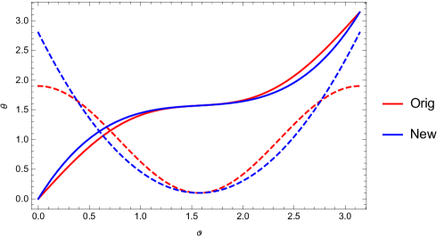
Figure 1: $\theta$-grid stretching functions comparing the transcendental function $\vartheta(\theta_{\rm KS})$ (solid red curves) with the cubic approach (solid blue curves) for $h=0.9$. We also give the respective derivatives $d\theta/d\vartheta$ (dashed).

With these transformations, we obtain the new metric $g_{\rm{MKS}}=J^{\mathrm{T}}g_{\rm{KS}}J$. Note that whenever the parameters $h=0$ and $R_{0}=0$ are set, our MKS coordinates reduce to the standard logarithmic Kerr-Schild coordinates.

2.7.2 Rezzolla & Zhidenko parametrization

The Rezzolla-Zhidenko parameterisation Rezzolla2014 has been proposed to describe spherically-symmetric BH geometries in metric theories of gravity. In particular, using a continued-fraction expansion (Padé expansion) along the radial coordinate, deviations from general relativity can be expressed using a small number of coefficients. The line element reads

$$ds^{2}=-N^{2}(r)dt^{2}+\frac{B^{2}(r)}{N^{2}(r)}dr^{2}+r^{2}d\theta^{2}+r^{2}\sin^{2}\theta d\phi^{2}\,,$$ (73)

with $N(r)$ and $B(r)$ being functions of the radial coordinate $r$. The radial position of the event horizon is fixed at $r=r_{0}>0$ which implies that $N(r_{0})=0$. Furthermore, the radial coordinate is compactified by means of the dimensionless coordinate

$$x:=1-\frac{r_{0}}{r}\,,$$ (74)

in which $x=0$ corresponds to the position of the event horizon, while $x=1$ corresponds to spatial infinity. Through this dimensionless coordinate, the function $N$ can be written as

$$N^{2}=x\,A(x)\,,$$ (75)

where $A(x)>0\quad\mbox{for}\quad 0\leq x\leq 1$. Introducing additional coefficients $\epsilon$, $a_{n}$, and $b_{n}$, the metric functions $A$ and $B$ are then expressed as follows

$$A(x) = 1-\epsilon(1-x)+(a_{0}-\epsilon)(1-x)^{2}+{\widetilde{A}}(x)(1-x)^{3}\,,$$ (76)

$$B(x) = 1+b_{0}(1-x)+{\widetilde{B}}(x)(1-x)^{2}\,.$$ (77)

Here ${\widetilde{A}}$ and ${\widetilde{B}}$ are functions describing the metric near the event horizon and at spatial infinity. In particular, ${\widetilde{A}}$ and ${\widetilde{B}}$ have rapid convergence properties, that is by Padé approximants

$${\widetilde{A}}(x)=\frac{a_{1}}{\displaystyle 1+\frac{\displaystyle a_{2}x}{\displaystyle 1+\frac{\displaystyle a_{3}x}{\displaystyle 1+\ldots}}}\,,\qquad\ {\widetilde{B}}(x)=\frac{b_{1}}{\displaystyle 1+\frac{\displaystyle b_{2}x}{\displaystyle 1+\frac{\displaystyle b_{3}x}{\displaystyle 1+\ldots}}}\,,$$ (78)

where $a_{1},a_{2},a_{3},\ldots$ and $b_{1},b_{2},b_{3},\ldots$ are dimensionless coefficients that can, in principle, be constrained from observations. The dimensionless parameter $\epsilon$ is fixed by the ADM mass $M$ and the coordinate of the horizon $r_{0}$. It measures the deviation from the Schwarzschild case as

$$\epsilon=\frac{2M-r_{0}}{r_{0}}=-\left(1-\frac{2M}{r_{0}}\right)\,.$$ (79)

It is easy to see that at spatial infinity ($x=1$), all coefficients contribute to (78), while at event horizon only the first two terms remain, i.e.

$${\tilde{A}}(0)={a_{1}}\,,\qquad{\tilde{B}}(0)={b_{1}}\,.$$ (80)

Given a number of coefficients, any spherical spacetime can hence directly be simulated in BHAC. For example, the coefficients in the Rezzolla-Zhidenko parametrization for the Johannsen-Psaltis (Johannsen2011, ) metric and for Einstein-Dilaton BHs (Garcia1995, ) have already been provided in Rezzolla2014 . Typically, expansion up to $a_{2},b_{2}$ yields sufficient numerical accuracy for the GRMHD simulations. The first simulations in the related horizon penetrating form of the Rezzolla-Zhidenko parametrization are discussed in Mizuno2017 .

2.8 Available reconstruction schemes

The second-order finite volume algorithm (56) requires numerical fluxes centered on the interface mid-point. As in any Godunov-type scheme (see e.g.,  Toro99, ; Komissarov1999, ), the fluxes are in fact computed by solving (approximate) Riemann problems at the interfaces (see Sect. 2.9). Hence for higher than first-order accuracy, the fluid variables need to be reconstructed at the interface by means of an appropriate spatial interpolation. Our reconstruction strategy is as follows. 1) Compute primitive variables $\boldsymbol{\bar{P}}$ from the averages of the conserved variables $\boldsymbol{\bar{U}}$ located at the cell barycenter. 2) Use the reconstruction formulae to obtain two representations for the state at the interface, one with a left-biased reconstruction stencil $\boldsymbol{P}^{\mathrm{L}}$ and the other with a right-biased stencil $\boldsymbol{P}^{\mathrm{R}}$. 3) Convert the now point-wise values back to their conserved states $\boldsymbol{U}^{\mathrm{L}}$ and $\boldsymbol{U}^{\mathrm{R}}$. The latter two states then serve as input for the approximate Riemann solver.

A large variety of reconstruction schemes are available, which can be grouped into standard second-order total variation diminishing (TVD) schemes like “minmod”, “vanLeer”, “monotonized-central”, “woodward” and “koren” (see Keppens2012, , for details) and higher order methods like the third-order methods “PPM” (Colella84, ), “LIMO3” (Cada2009, ) and the fifth-order monotonicity preserving scheme “MP5” due to (suresh_1997_amp, ). While the overall order of the scheme will remain second-order, the higher accuracy of the spatial discretisation usually reduces the diffusion of the scheme and improves accuracy of the solution (see, e.g.,  Porth2014, ). For typical GRMHD simulations with near-evacuated funnel/atmosphere regions, we find the PPM reconstruction scheme to be a good compromise between high accuracy and robustness. For simple flows, e.g., the stationary toroidal field torus discussed in Sect. 3.4, the compact stencil LIMO3 method is recommended.

2.9 Characteristic speed and approximate Riemann solvers

The time-update of BHAC proceeds in a dimensionally unsplit manner, thus at each Runge-Kutta substep the interface-fluxes in all directions are computed based on the previous substep. The state is then advanced to the next substep with the combined fluxes of the cell. To compute these fluxes from the reconstructed conserved variables at the interface $\boldsymbol{U}^{L}$ and $\boldsymbol{U}^{R}$, we provide two approximate Riemann solvers: 1) the Rusanov flux, also known as Total variation diminishing Lax-Friedrichs scheme (TVDLF) which is based on the largest absolute value of the characteristic waves normal to the interface $c^{i}$, and 2) the HLL solver (Harten83, ), which is based on the leftmost ($c_{-}^{i}$) and rightmost ($c_{+}^{i}$) waves of the characteristic fan with respect to the interface. The HLL upwind flux function for the conserved variable $u\in\boldsymbol{U}$ is calculated as

$$F^{i}(u)=\left\{\begin{array}[]{lcc}F^{i}(\boldsymbol{U}^{\mathrm{L}})&;&c_{-}^{i}>0\\ F^{i}(\boldsymbol{U}^{\mathrm{R}})&;&c_{+}^{i}<0\\ \tilde{F}^{i}(\boldsymbol{U}^{\mathrm{L}},\boldsymbol{U}^{\mathrm{R}})&;&{\rm otherwise}\\ \end{array}\right.$$ (81)

where

$$\tilde{F}^{i}(\boldsymbol{U}^{\mathrm{L}},\boldsymbol{U}^{\mathrm{R}}):=\frac{c_{+}^{i}\,F^{i}\left(\boldsymbol{U}^{\mathrm{L}}\right)-c_{-}^{i}\,F^{i}\left(\boldsymbol{U}^{\mathrm{R}}\right)+c_{+}^{i}\,c_{-}^{i}\,\left(u^{\mathrm{R}}-u^{\mathrm{L}}\right)}{c_{+}^{i}\,-\,c_{-}^{i}}\,,$$ (82)

and we set in accordance with Davis1988 : $c_{-}^{i}={\rm min}\left(\lambda_{i,-}^{\mathrm{L}},\lambda_{i,-}^{\mathrm{R}}\right)$, $c_{+}^{i}={\rm max}\left(\lambda_{+}^{\mathrm{L}},\lambda_{+}^{\mathrm{R}}\right)$.

The TVDLF flux is simply

$$F^{i}(u)=\frac{1}{2}\left[F^{i}(\boldsymbol{U}^{\mathrm{L}})+F^{i}(\boldsymbol{U}^{\mathrm{R}})\right]-\frac{1}{2}c^{i}\left(u^{\mathrm{R}}-u^{\mathrm{L}}\right)\,.$$ (83)

with $c^{i}={\rm max}\left(|c_{-}^{i}|,|c_{+}^{i}|\right)\,$.

In addition to these two standard approximate Riemann solvers, we also provide a modified TVDLF solver that preserves positivity of the conserved density $D$. The algorithm was first described in the context of Newtonian hydrodynamics by Hu2013 and was successfully applied in GRHD simulations by Radice2013c . It takes advantage of the fact that the first-order Lax-Friedrichs flux $F^{i,\mathrm{LO}}(u)$ is positivity preserving under a CFL condition ${\rm CFL}\leq 1/2$. Hence the fluxes can be constructed by combining the high order flux $F^{i,\mathrm{HO}}(u)$ (obtained e.g., by PPM reconstruction) and $F^{i,\mathrm{LO}}(u)$ such that the updated density does not fall below a certain threshold. Specifically, the modified fluxes read

$$F^{i}(u)=\theta F^{i,\mathrm{HO}}(u)+(1-\theta)F^{i,\mathrm{LO}}(u)\,,$$ (84)

where $\theta\in[0,1]$ is chosen as a maximum value which ensures positivity of the cells adjacent to the interface (see Hu2013 for details of its construction). Note that although we only stipulate the density be positive, the formula (84) must be applied to all conserved variables $u\in\boldsymbol{U}$.

In relativistic MHD, the exact form of the characteristic wave speeds $\lambda_{\pm}$ involves solution of a quartic equation (see, e.g.,  Anile1990, ) which can add to the computational overhead. For simplicity, instead of calculating the exact characteristic velocities, we follow the strategy of Gammie03 who propose a simplified dispersion relation for the fast MHD wave $\omega^{2}=a^{2}k^{2}$. As a trade-off, the simplification can overestimate the wavespeed in the fluid frame by up to a factor of $2$, yielding a slightly more diffusive behaviour. The upper bound $a$ for the fast wavespeed is given by

$$a^{2}=c_{s}^{2}+c_{a}^{2}-c_{s}^{2}c_{a}^{2}\,,$$ (85)

which depends on the usual sound speed and Alfvén speed

$$c_{s}^{2}=\hat{\gamma}\frac{p}{\rho h}\,,\qquad c_{a}^{2}=\frac{b^{2}}{\rho h+b^{2}}\,,$$ (86)

here given for an ideal EOS with adiabatic index $\hat{\gamma}$. As pointed out by DelZanna2007 , the 3+1 structure of the fluxes leads to characteristic waves of the form

$$\lambda_{\pm}^{i}=\alpha\,\lambda_{\pm}^{{}^{\prime}i}-\beta^{i}\,,$$ (87)

where $\lambda_{\pm}^{{}^{\prime}i}$ is the characteristic velocity in the corresponding special relativistic system ($\alpha\to 1$, $\beta^{i}\to 0$).

For the simplified isotropic dispersion relation, the characteristics can then be obtained just like in special relativistic hydrodynamics (see, e.g.,  Font1994, ; Banyuls97, ; Keppens2008, )

$$\lambda_{\pm}^{{}^{\prime}i}= \frac{\left(1-a^{2}\right)\,v^{i}\pm\sqrt{a^{2}\,\left(1-v^{2}\right)\,\left[\left(1-v^{2}a^{2}\right)\gamma^{ii}-\left(1-a^{2}\right){\left(v^{i}\right)}^{2}\right]}}{(1-v^{2}\,a^{2})}.$$ (88)

2.10 Primitive variable recovery

It is well-known that the nonlinear inversion $\boldsymbol{P}(\boldsymbol{U})$ is the Achilles heel of any relativistic (M)HD code and sophisticated schemes with multiple backup strategies have been developed over the years as a consequence (e.g., Noble2006 , Faber2007 , Noble2009 , Etienne2012 , Galeazzi2013 , Hamlin2013 ). Here we briefly describe the methods used throughout this work and refer to the previously mentioned references for a more detailed discussion.

2.10.1 Primary inversions

Two primary inversion strategies are available in BHAC. The first strategy, which we denote by “1D”, is a straightforward generalisation of the one-dimensional strategy described in (vanderHolst2008, ). It involves a non-linear root finding algorithm which is implemented by means of a Newton-Raphson scheme on the auxiliary variable $\xi$. Once $\xi$ is found, the velocity follows from (41)

$$v^{i}=\frac{S^{i}}{(\xi+B^{2})}+\frac{B^{i}(B^{j}S_{j})}{\xi(\xi+B^{2})}\,,$$ (89)

and we calculate the second auxiliary variable $\Gamma=(1-v^{2})^{-1/2}$ so that $\rho=D/\Gamma$. The thermal pressure $p$ then follows from the particular EOS in use (Sect. 2.4). For example, for an ideal EOS we have

$$p=\frac{\hat{\gamma}}{\hat{\gamma}-1}\left(\frac{\xi}{\Gamma^{2}}-\rho\right)\,.$$ (90)

For details of the consistency checks and bracketing, we refer the interested reader to vanderHolst2008 .

In addition to the 1D scheme, we have implemented the “2DW” method of Noble2006 ; DelZanna2007 . The 2DW inversion simultaneously solves the non-linear equations (37) and the square of the three-momentum $S^{2}$, following (41) by means of a Newton-Raphson scheme on the two variables $\xi$ and $v^{2}$. Among all inversions tested by Noble2006 , the 2DW method was reported as the one with the smallest failure rate. We find the same trend, but also find that the lead of 2DW over 1D is rather minor in our tests.

With two distinct inversions that might fail under different circumstances, one can act as a backup strategy for the other. Typically we first attempt a 2DW inversion and switch to the 1D method when no convergence is found. The next layer of backup can be provided by the entropy method as described in the next section.

2.10.2 Entropy switch

To deal with highly magnetised regions, Noble2009 ; Sadowski2013 introduced the advection of entropy to provide a backup strategy for the primitive variable recovery. Similar to Noble2009 ; Sadowski2013 , alongside the usual fluid equations, BHAC can be configured to solve an advection equation for the entropy $S$

$$\nabla_{\mu}Su^{\mu}=0\,,$$ (91)

where we define

$$S:=p/\rho^{\hat{\gamma}-1}\,,$$ (92)

given the adiabatic index $\hat{\gamma}$. This leads to the evolution equation

$$\partial_{t}\sqrt{\gamma}\Gamma S+\partial_{i}\sqrt{\gamma}(\alpha v^{i}-\beta^{i})\Gamma S=0\,,$$ (93)

for the conserved quantity $\Gamma S$. The primitive counterpart is the actual entropy $\kappa=p/\rho^{\hat{\gamma}}$, which can be recovered via $\kappa=\Gamma S/D$. In case of failure of the primary inversion scheme, using the advected entropy $\kappa$, we can attempt a recovery of primitive variables which does not depend on the conserved energy. Note that after the primitive variables are recovered from the entropy, we need to discard the conserved energy and set it to the value consistent with the entropy. On the other hand, after each successful recovery of primitive variables, the entropy is updated to $\kappa=p/\rho^{\hat{\gamma}}$, which is then advected to the next step. In addition, entropy-based inversion can be activated whenever $\beta=2p/b^{2}\leq 10^{-2}$ since the primary inversion scheme is likely to fail in these highly magnetised regions. Tests of the dynamic switching of the evolutionary equations are described in Sect. 3.3. In GRMHD simulations of BH accretion, the “entropy region” is typically located in the BH magnetosphere, which is strongly magnetised and the error due to missing shock dissipation is thus expected to be small.

In the rare instances where the entropy inversion also fails to converge to a physical solution, the code is normally stopped. To force a continuation of the simulation, last resort measures that depend on the physical scenario can be employed. Often the simulation can be continued when the faulty cell is replaced with averages of the primitive variables of the neighbouring healthy cells as described in Keppens2012 . In the GRMHD accretion simulations described below, failures could happen occasionally in the highly magnetised evacuated “funnel” region close to the outer horizon where the floors are frequently applied. We found that the best strategy is then to replace the faulty density and pressure values with the floor values and set the Eulerian velocity to zero. Note that in order to avoid generating spurious $\boldsymbol{\nabla\cdot B}$, the last resort measures should never modify the magnetic fields of the simulation.

2.11 Adaptive Mesh refinement

The computational grid employed in BHAC is provided by the MPI-AMRVAC toolkit and constitutes a fully adaptive block based (oct-) tree with a fixed refinement factor of two between successive levels. That is, the domain is first split into a number of blocks with equal amount of cells (e.g., $10^{3}$ computational cells per block). Each block can be refined into two (1D), four (2D) or eight (3D) child-blocks with an again fixed number of cells. This process of refinement can be repeated ad libitum and the data-structure can be thought of a forest (collection of trees). All operations on the grid, for example time-update, IO and problem initialisation are scheduled via a loop over a space-filling curve. We adopt the Morton Z-order curve for ease of implementation via a simple recursive algorithm.

Currently, all cells are updated with the same global time-step and hence load-balancing is achieved by cutting the space-filling curve into equal sections that are then distributed over the MPI-processes. The AMR strategy just described is applied in various astrophysical codes, for example codes employing the PARAMESH library MacNeice00 ; Fryxell2000 ; Zhang2006 , or the recent Athena++ framework (see, e.g.,  White2016, ). Compared to a patch-based approach (see, e.g.,  Mignone2012, ), the block based AMR has several advantages: 1) well-defined boundaries between neighbouring grids on different levels ,2) data is uniquely stored and updated, thus no unnecessary interpolations are performed, and 3) simple data-structure, e.g., straightforward integer arithmetic can be used to locate a particular computational block. For in-depth implementation details such as refinement/prolongation operations, indexing and ghost-cell exchange, we refer to Keppens2012 . Prolongation and restriction can be used on conservative variables or primitive variables. Typically primitive variables are chosen to avoid unphysical states which can otherwise result from the interpolations in conserved variables. The refinement criteria usually adapted is the Löhner’s error estimator Loehner87 on physical variables. It is a modified second derivative, normalised by the average of the gradient over one computational cell. The multidimensional generalization is given by

$$E_{i_{1}i_{2}i_{3}}=\sqrt{\frac{\sum_{p}\sum_{q}\left({\partial^{2}u\over\partial x_{p}\partial x_{q}}\Delta x_{p}\Delta x_{q}\right)^{2}}{\sum_{p}\sum{q}\left[\left(\left|{\partial u\over\partial x_{p}}\right|_{i_{p}+1/2}+\left|{\partial u\over\partial x_{p}}\right|_{i_{p}-1/2}\right)\Delta x_{p}+f_{\rm wave}{\partial^{2}|u|\over\partial x_{p}\partial x_{q}}\Delta x_{p}\Delta x_{q}\right]^{2}}}.$$ (94)

The indices $p,q$ run over all dimensions $p,q=1,...,N_{D}$. The last term in the denominator acts as a filter to prevent refinement of small ripples, where $f_{\rm wave}$ is typically chosen of order $10^{-2}$. This method is also used in other AMR codes such as FLASH (Calderetal02, ), RAM (Zhang2006, ), PLUTO (Mignone2012, ) and ECHO (Zanotti2015b, ).

3 Numerical tests

3.1 Shock tube test with gauge effect

The first code test is considered in flat spacetime and therefore no metric source terms are involved. Herein we perform one-dimensional MHD shock tube tests with gauge effects by considering gauge transformations of the spacetime. Shock tube tests are well-known tests for code validation and emphasise the nonlinear behaviour of the equations, as well as the ability to resolve discontinuities in the solutions (see, e.g.,  Anton05, ; DelZanna2007, ).

The initial condition is given as

$$\begin{split}(\rho,p,B^{x},B^{y})=\left\{\begin{array}[]{ll}(1,1,0.5,1)&x<0\,,\\ (0.125,0.1,0.5,-1)&x>0\,,\end{array}\right.\end{split}$$ (95)

and all other quantities are zero. In order to check whether the covariant fluxes are correctly implemented, we use different settings for the flat spacetime as detailed in Table 3.

Table 3: Shock tube with gaugeeffect setups.

Case	$\alpha$	$\beta^{i}$	$\gamma_{11}$	$\gamma_{22}$	$\gamma_{33}$
A	1	(0,0,0)	1	1	1
B	2	(0,0,0)	1	1	1
C	1	(0.4,0,0)	1	1	1
D	1	(0,0,0)	4	1	1
E	1	(0,0,0)	1	4	1
F	2	(0.4,0,0)	4	9	1

In the simulations, an ideal gas EOS is employed with an adiabatic index of $\hat{\gamma}=2$. The 1D problem is run on a uniform grid in $x-$direction using 1024 cells spanning over $x\in[-1/2,1/2]$. The simulations are terminated at $t=0.4$. For the spatial reconstruction, we adopt the second order TVD limiter due to Koren (Koren1993, ). Furthermore, RK3 timeintegration is used with Courant number set to $0.4$.

Case A is the reference solution without modification of fluxes due to the three-metric, lapse or shift. By means of simple transformations of flat-spacetime, all other cases can be matched with the reference solution. Case B will coincide with solution A if B is viewed at $t/2=0.2$. Case C will agree with case A when it is shifted in positive $x-$direction by $\delta x=\beta^{x}t=0.16$. For case D, we rescale the domain as $x\in[-1/4,1/4]$ and initialise the contravariant vectors as $B^{\prime x}=B^{x}/2$. The state at $t=0.4$ should agree with case A when the domain is multiplied by the scale factor $h_{x}=2$. For case E we initialise $B^{\prime y}=B^{y}/2$ and case F is initialised similarly as $B^{\prime x}=B^{x}/2$, $B^{\prime y}=B^{y}/3$.

In general, all cases agree very well with the rescaled solution. To give an example, Fig. 2 shows the rescaled simulation results of case F compared to the reference solution of case A. This test demonstrates the shock-capturing ability of the MHD code and enables us to conclude that the calculation of the covariant fluxes has been implemented correctly.

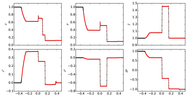
Figure 2: 1D plots of density $\rho$, gas pressure $p$, Lorentz factor $\Gamma$, velocity components $v^{x}$ and $v^{y}$, and the $y$-component of the magnetic field for the shock tube test at $t=0.4$. The reference solution of case A is shown as a solid black line and the rescaled solution of case F is overplotted as red squares.

3.2 Boosted loop advection

In order to test the implementation of the GLM-GRMHD system, we perform the advection of a force-free flux-tube with poloidal and toroidal components of the magnetic field in a flat spacetime.

The initial equilibrium configuration of a force-free flux-tube is given by a modified Lundquist tube (see e.g.,  Gourgouliatos2012, ), where we avoid sign changes of the vertical field component $B^{z}$ with the additive constant $C=0.01$. Pressure and density are initialized as constant throughout the simulation domain. The initial pressure value is obtained from the central plasma-beta $\beta_{0}=B^{2}(0)/2p$, where $B$ is the magnetic field in the co-moving system. The density is set to $\rho=p/2$ yielding a relativistic hot plasma. Consequently, an adiabatic index $\gamma=4/3$ is used. We set $\beta_{0}=0.01$, which results in a high magnetisation $\sigma_{0}=B^{2}(0)/(\rho c^{2}+4p)\simeq 25$. The equations for the magnetic field for $r<1$ read

$$B^{\phi}(r) =J_{1}(\alpha_{t}r)\,,$$ (96)

$$B^{z}(r) =\sqrt{J_{0}(\alpha_{t}r)^{2}+C}\,,$$ (97)

and

$$B^{\phi}(r) =0\,,$$ (98)

$$B^{z}(r) =\sqrt{J_{0}(\alpha_{t})^{2}+C}\,,$$ (99)

otherwise, where $J_{0}$ and $J_{1}$ are Bessel functions of zeroth and first order respectively and the constant $\alpha_{t}\simeq 3.8317$ is the first root of $J_{0}$.

This configuration is then boosted to the frame moving at velocity $\boldsymbol{v}=\sqrt{2}(-v_{c},-v_{c},0)$ and we test values of $v_{c}$ between $0.5$c and $0.99$c.

Standard Lorentz transformation rules result in

$$\boldsymbol{r}=\boldsymbol{r}^{\prime}+(\Gamma-1)(\boldsymbol{r^{\prime}\cdot n})\boldsymbol{n}-\Gamma t^{\prime}v_{c}\boldsymbol{n}\,,\ \hskip 28.45274pt\boldsymbol{B}^{\prime}=\Gamma\boldsymbol{B}-\frac{\Gamma^{2}}{\Gamma+1}\boldsymbol{\beta}(\boldsymbol{\beta\cdot B})\,,$$ (100)

where $t^{\prime}$ can be set to zero and where we assumed a vanishing electric field in the co-moving system. Therefore relativistic length contraction gives the loop a squeezed appearance. A simulation domain $(x,y)\in[-1,1]$ at a base resolution of $N_{x}\times N_{y}=64^{2}$ is initialised with an additional three levels of refinement. We advect the loop for one period ($P=2\sqrt{2}/v$) across the domain where periodic boundary conditions are used.

The advection over the coordinates can be counteracted by setting the shift vector appropriately, i.e. $\boldsymbol{\beta}=-\boldsymbol{v}$. This is an important consistency check of the implementation. Figure 3 shows the initial and final states of the force-free magnetic flux-tube advected for one period and for the case with spacetime shifted against the advection velocity. The advected and counter-shifted cases are in good agreement, with only the truly advected case being slightly more diffused, the effect of which is reflected in the activation of more blocks on the third AMR level.

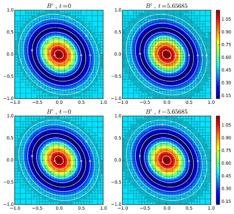
Figure 3: Force-free magnetic loop with diagonal boost velocity $|v|=0.5c$. Top: No shift, the loop is advected for one period. Bottom: The shift vector just opposes the (diagonal) advection velocity, $|v|=0.5$, hence the loop remains stationary with respect to the grid. Base resolution is $64^{2}$ cells with a total of three grid levels. The color shows the strength of the out-of-plane field component $B^{z}$ and white lines are in-plane field lines of $(B^{x},B^{z})$. Blocks containing $8^{2}$ cells are indicated.

To investigate the numerical accuracy the $L_{1}$ and $L_{\infty}$ norms of the out-of-plane magnetic field component $B^{z}$, as well as the divergence of magnetic field between the initial state and the simulation at a time after one advection period with different resolutions as seen in Fig.4 are checked. The error norms from analytically known solutions $u^{*}$ are defined as

$$L_{1}(u) =\frac{1}{N_{\rm cells}}\sum_{i,j,k}\left|\bar{u}_{i,j,k}-\frac{1}{\Delta V_{i,j,k}}\int_{V_{i,j,k}}u^{*}\sqrt{\gamma}dx^{1}dx^{2}dx^{3}\right|\,,$$ (101)

$$L_{\infty}(u) ={\rm max}_{i,j,k}\left|\bar{u}_{i,j,k}-\frac{1}{\Delta V_{i,j,k}}\int_{V_{i,j,k}}u^{*}\sqrt{\gamma}dx^{1}dx^{2}dx^{3}\right|\,,$$ (102)

where the summation, respectively maximum operation, includes all cells in the domain and the integrals are performed over the volume of the cell $\Delta V_{i,j,k}$. In this sense, the reported errors correspond to the mean and maximal error in the computational domain. We should note that for the test of convergence, we use a uniform grid and choose $\boldsymbol{v}=0.5\sqrt{0.5}(1,1,0),\beta=\sqrt{0.5}(1,0,0)$ resulting in an advection in direction of the upper-left diagonal. A TVD “Koren” limiter is chosen. As expected, the convergence is second order for all cases.

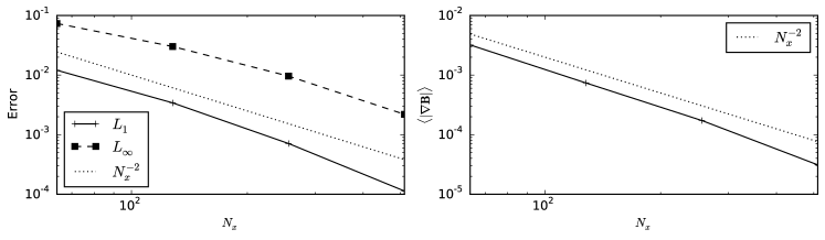
Figure 4: Error of the out-of-plane magnetic field component $B^{z}$ (left) and divergence of $\boldsymbol{B}$ (right). For this test, we chose $\boldsymbol{v}=0.5\sqrt{0.5}(1,1,0)$ and $\beta=\sqrt{0.5}(1,0,0)$, resulting in an advection in the direction of the upper-left diagonal.

3.3 Magnetised spherical accretion

A useful stress test for the conservative algorithm in a general-relativistic setting is spherical accretion onto a Schwarzschild BH with a strong radial magnetic field Gammie03 . The steady-state solution is known as the Michel accretion solution (Michel72, ) and represents the extension to general relativity of the corresponding Newtonian solution by Bondi52 . The steady-state spherical accretion solution in general relativity is described in a number of works (see, e.g.,  Hawley84a, ; Rezzolla_book:2013, ). It is easy to show that the solution is not affected when a radial magnetic field of the form $B^{r}\propto\gamma^{-1/2}$ is added (DeVilliers03a, ). This test challenges the robustness of the code and of the inversion procedure $\boldsymbol{P}(\boldsymbol{U})$ in particular. The calculation of the initial condition follows that outlined in Hawley84a . Here, we parametrize the field strength via $\sigma=b^{2}/\rho$ at the inner edge of the domain ($r=1.9\,M$). The simulation is setup in the equatorial plane using MKS coordinates corresponding to a domain of $r_{\rm KS}\in[1.9,20]\,M$. The analytic solution remains fixed at the inner and outer radial boundaries. We run two cases, case 1 with magnetisation up to $\sigma=10^{3}$ and case 2 with a very high magnetisation reaching up to $\sigma=10^{4}$. Since the problem is only 1D, the constraint $\mathbf{\nabla\cdot B}=0$ has a unique solution which gets preserved via the FCT algorithm.

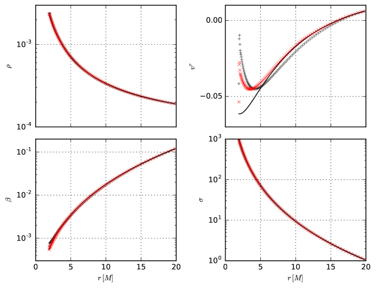
Figure 5: Magnetized Bondi flow at $t=100\,M$ in MKS coordinates with $\sigma=10^{3}$ at the inner edge of the domain. The black solid curve indicates the initial exact solution. We show two realisations with resolution $N_{r}=100$. Black crosses are with the standard treatment for the inversion. Red crosses switch to the entropy evolution at $\beta\leq 10^{-2}$ (here in the middle of the domain). In particular, the error in the radial three-velocity $v^{r}$ decreases when switching to the entropy evolution.

Figure 5 illustrates the profiles for $\sigma=10^{3}$ and two inversion strategies: 2DW (black $+$) and 2DW with entropy switching in regions of high magnetization $b^{2}/2p>100$ (red $\times$). With the exception of the radial three-velocity near the BH horizon ($r\leq 5\,M$), in both cases the simulations maintain well the steady-state solution. Comparing theses results with and without entropy switching, the entropy strategy actually keeps the solution closer to the steady-state solution (solid black curves) even though the change of inversion strategy occurs in the middle of the domain, $r\simeq 10$.

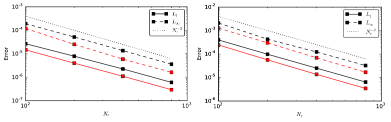
Figure 6: Error of density $\rho$ in the highly magnetised Bondi flow: $\sigma=10^{3}$ (left) and $\sigma=10^{4}$ (right). The black data points are obtained with the standard 2D inversion and the red datapoints switch to the entropy inversion at $\beta\leq 10^{-2}$. One can see that both recipes are convergent with the expected order and that the error in the entropy strategy is decreased by roughly a factor of two.

The errors ($L_{1}$ and $L_{\infty}$ norms) for the four cases are shown in Fig. 6. Again, the second-order accuracy of the algorithm is recovered. Using the entropy strategy increases the numerical accuracy by around a factor of two and we suggest its use in the highly magnetised regime of BH magnetospheres.

3.4 Magnetised equilibrium torus

As a final validation of the code in the GRMHD regime, we perform the simulation of a magnetised equilibrium torus around a spinning BH. A generalisation of the steady-state solution of the standard hydrodynamical equilibrium torus with constant angular momentum (see, e.g.,  Fishbone76, ; Hawley84a, ; Font02a, ) to MHD equilibria with toroidal magnetic fields was proposed by Komissarov2006a . This steady-state solution is important since it constitutes a rare case of a non-trivial analytic solution in GRMHD.

For the initial setup of the equilibrium torus, we adopt a particular relationship $\omega=\omega(p)$, where $\omega=\rho h$ is the fluid enthalpy and $\tilde{\omega}=\tilde{\omega}(\tilde{p_{m}})$, where $\tilde{p}_{m}=\mathcal{L}p_{m}$, $\tilde{\omega}=\mathcal{L}\omega$, $p_{m}=b^{2}/2$ is the magnetic pressure, and $\mathcal{L}=g_{t\phi}g_{t\phi}-g_{tt}g_{\phi\phi}$. From these relationships, thermal and magnetic pressures are described as

$$p =K\omega^{\kappa}\,,$$ (103)

$$\tilde{p}_{m} =K_{m}\tilde{\omega}^{\eta}\,.$$ (104)

The analytical solutions can be constructed from

$$W-W_{in}+{\kappa\over\kappa-1}{p\over\omega}+{\eta\over\eta-1}{p_{m}\over\omega}=0\,,$$ (105)

for the introduced total potential $W$, where $W=\ln|u_{t}|$. The centre of the torus is located at $(r_{\mathrm{c}},\pi/2)$. At this point, we parametrize the magnetic field strength in terms of the pressure ratio

$$\beta_{c}=p_{g}(r_{c},\pi/2)/p_{m}(r_{c},\pi/2)\,.$$ (106)

The gas pressure and magnetic pressure at the centre of the torus are given by

$$p_{c}=\omega_{c}(W_{in}-W_{c})\left({\kappa\over\kappa-1}+{\eta\over\eta-1}{1\over\beta_{c}}\right)^{-1}\,,\qquad p_{m_{c}}=p_{c}/\beta_{c}\,.$$ (107)

From these, the constants $K$ and $K_{m}$ for barotropic fluids are obtained.

The magnetic field distribution is given by the distribution of magnetic pressure $p_{\mathrm{m}}$. From the consideration of a purely toroidal magnetic field one obtains

$$b^{\phi}=\sqrt{2p_{m}/\mathcal{A}}\,,\qquad\ b^{t}=\ell\,b^{\phi}\,,$$ (108)

where $\mathcal{A}=g_{\phi\phi}+2lg_{t\phi}+l^{2}g_{tt}$ and $\ell:=-u_{\phi}/u_{t}$ is the specific angular momentum.

We perform 2D simulations using logarithmic KS coordinates with $h=0$ and $R_{0}=0$. The simulation domain is $\theta\in[0,\pi]$, $r_{\rm KS}\in[0.95\,r_{\mathrm{h}},\ 50\,M]$, where $r_{\mathrm{h}}$ is the (outer) event horizon radius of the BH. The BH has the dimensionless spin parameter $a=0.9$. For simplicity, we set the two indices to the same value of $\kappa=\eta=4/3$ and also set the adiabatic index of the adopted ideal EOS to $\gamma=4/3$. The remaining parameters are listed in the Table 4.

Table 4: Parameters for the MHD equilibrium torus test

Case	$l_{0}$	$r_{c}$	$W_{in}$	$W_{c}$	$\omega_{c}$	$\beta_{c}$
A	2.8	4.62	-0.030	-0.103	1.0	0.1

Initially, the velocity of the atmosphere outside of the torus is set to zero in the Eulerian frame, with density and gas pressure set to very small values of $\rho=\rho_{\mathrm{min}}\,r_{\rm BL}^{-3/2}$, $p=p_{\mathrm{min}}\,r_{\rm BL}^{-5/2}$ with $\rho_{\mathrm{min}}=10^{-5}$ and $p_{\mathrm{min}}=10^{-7}$. It is important to note that the atmosphere is free to evolve and only densities and pressures are floored according to the initial state. In the simulations we use the HLL approximate Riemann solver, third order LIMO3 reconstruction, two-step time update, and a CFL number of $0.5$. We impose outflow conditions on the inner and outer boundaries of the radial direction and reflecting boundary conditions in the $\theta$ direction. As the magnetic field is purely toroidal, and will remain so during the time-evolution of this axisymmetric case, no particular $\mathbf{\nabla\cdot B=0}$ treatment is used.

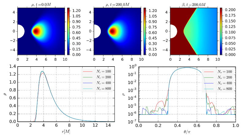
Figure 7: Top: qualitative view of the torus evolution at a resolution of $N_{r}=N_{\theta}=400$. The spatial scale is given in units of $M$. Left: Initial rest-frame density distribution, center: density at $t=200\,M$, right: plasma $\beta$ parameter at $t=200\,M$. Bottom: density slices through the torus at $t=100\,M$ for constant $\theta=\pi/2$ (left) and $r=5$ (right).

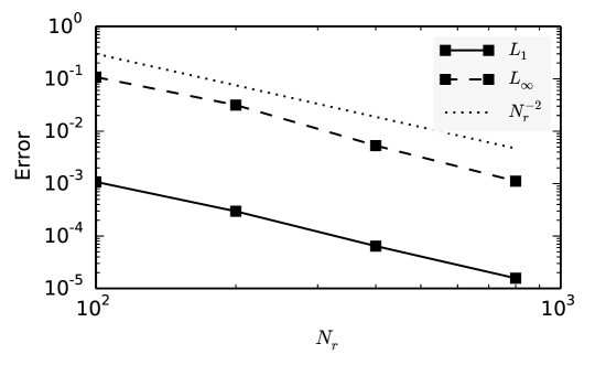
Figure 8: Error of the density $\rho$ in the strongly-magnetised Komissarov torus, comparing the solution at $t=60\,M$ with the exact solution. The second-order behaviour of the numerical scheme is well recovered.

The top panels of Fig. 7 show the density distribution at the initial state and at $t=200\,M$, as well as the plasma beta distribution at $t=200\,M$. The rotational period of the disk centre is $t_{\mathrm{r}}=68\,M$. The initial torus configuration is well maintained after several rotation period. For a qualitative view of the simulations, the 1D radial and azimuthal distributions of the density are shown in the lower two panels in Fig. 7 with different grid resolutions. All but the low resolution case are visually indistinguishable from the initial condition in the bottom-left panel, showing $\rho-r$ with a linear scale. Since the atmosphere is evolved freely, small density waves propagate in the ambient medium of the torus, as seen in the $\rho-\theta$ cut. This does not adversely affect the equilibrium solution in the bulk of the torus however. Error quantification ($L_{1}$ and $L_{\infty}$) is provided in Fig. 8. The second-order properties of the numerical scheme are well recovered.

3.5 Differences between FCT and GLM

Having implemented two methods for divergence control, we took the opportunity to compare the results of simulations using both methods. We analysed three tests: a relativistic Orszag-Tang vortex, magnetised Michel accretion, and magnetised accretion from a Fishbone-Moncrief torus. Although much less in-depth, this comparison is in the same spirit as those performed in previous works in non-relativistic MHD Toth2000 ; Balsara2004 ; Mocz2016 . The well-known work by Toth2000 compares seven divergence-control methods, including an early non-conservative divergence-cleaning method known as the eight-wave method Powell1994 , and three CT methods, finding that FCT is among the three most accurate schemes for the test problems studied. In Balsara2004 , three divergence-cleaning schemes and one CT scheme were applied to the same test problem of supernova-induced MHD turbulence in the interstellar medium. It was found that the three divergence-cleaning methods studied suffer from, among other problems, spurious oscillations in the magnetic energy, which is attributed to the non-locality introduced by the loss of hyperbolicity in the equations. Finally, in Mocz2016 , a non-staggered version of CT adapted to a moving mesh is compared to the divergence-cleaning Powell scheme Powell1999 , an improved version of the eight-wave method. They observe greater numerical stability and accuracy, and a better preservation of the magnetic field topology for the CT scheme. In their tests, the Powell scheme suffers from an artificial growth of the magnetic field. This is explained to be a result of the scheme being non-conservative.

3.5.1 Orszag-Tang Vortex

The Orszag-Tang vortex Orszag1979 is a common problem that can be used to test MHD codes for violations of $\nabla\cdot\boldsymbol{B}$. The relativistic version presented here was performed in 2D using Cartesian coordinates in a $128\times 128$-resolution domain of $2\pi\times 2\pi$ length units with periodic boundary conditions, and evolved for $10$ time units ($c=1$). The equation of state was chosen to be that of an ideal fluid with $\hat{\gamma}=4/3$ and the initial conditions were set to $\rho=1.0$, $p=10.0$, $v^{x}=-0.99\sin y$, $v^{y}=0.99\sin x$, $B^{x}=-\sin y$ and $B^{y}=\sin 2x$ . Snapshots of the evolution are shown in Fig. 9.

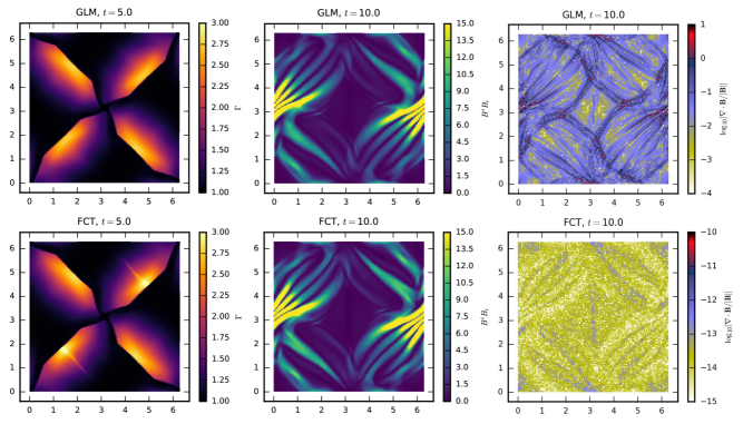
Figure 9: Relativistic Orszag-Tang vortex. Left column: small differences can be observed in this snapshot of the Lorentz factor at $t=5.0$. Some features that appear when using CT are flattened when using GLM, possibly due to a greater diffusivity of the latter. Middle column: final snapshot of $B^{i}B_{i}$. Good agreement between the two methods can be seen, except at some extreme points. Right column: violation of $\nabla\cdot\boldsymbol{B}=0$.

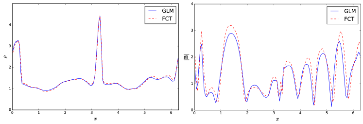
Figure 10: Relativistic Orszag-Tang vortex: cuts at $y=\pi/2$ and $t=10.0$ of the density $\rho$ (left) and the magnitude of the magnetic field $|B|$ (right). While for $\rho$ there is in general a good agreement, FCT tends to produce higher maxima for the magnetic field.

As can be seen in Figs. 9 and  10, the general behaviour in both cases is quite similar qualitatively, with only slight differences at specific locations. For instance, when compared to GLM, FCT exhibited higher and sharper maxima for the magnitude of the magnetic field. In a similar fashion, some fine features in the Lorentz factor that can be seen in Fig.  9 for FCT appear to be smeared out when using GLM, giving a false impression of symmetry under 90^∘ rotations, while the actual symmetry of the problem is under 180^∘ rotations. This may be an evidence of FCT being less diffusive than GLM.

3.5.2 Spherical accretion

We tested the ability of both methods to preserve a stationary solution by evolving a magnetised Michel accretion in 2D, as shown in Fig. 11.

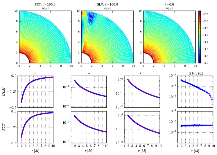
Figure 11: Top: logarithmic density and streamlines in 2D magnetised Michel accretion at times $t=0\,M$ (left) and $t=100\,M$ using GLM (centre) and FCT (right). The horizon is marked by the black line at $r=2$. Bottom: profiles at $\theta=\pi/2$ of, from left to right, radial 3-velocity, density and radial magnetic field at $t=0\,M$ (blue circles) and $t=100\,M$ (red line) using GLM (upper) and FCT (lower). The last column shows the relative difference between the magnetic field at $t=100\,M$ and at the initial condition.

We employed spherical MKS coordinates (see Sect.  2.7.1), $N_{r}\times N_{\theta}=200\times 100$ resolution, and a domain with $r\in[1.9M,10M]$ and $\theta\in[0,\pi]$. The fluid obeyed an ideal equation of state with $\hat{\gamma}=5/3$ and the sonic radius was located at $r_{\mathrm{c}}=8$, and the magnetic field was normalised so that the maximum magnetisation was $\sigma=10^{3}$. We repeated the numerical experiment of section Sect. 3.3, now in 2D. As shown in Fig. 11, numerical artefacts start to become noticeable at these later times. For instance, with these extreme magnetisations, for GLM we observe spurious features near the poles at $\theta=0$ and $\theta=\pi$, as well as deviations in the velocity field near the outer boundary $r=10\,M$. The polar region is of special interest for jet simulations, where the divergence-control method must be robust enough to interplay with the axial boundary conditions. The bottom of Fig. 11 shows the profiles of several quantities at $\theta=\pi/2$. Both divergence-control methods produce an excellent agreement between the solution at different times in the equatorial region. The rightmost column in the bottom of Fig. 11 shows the relative errors in the radial component of the magnetic field for each method. The errors for FCT are not only one order of magnitude lower than for GLM, but also behave differently, remaining at the same level near the more-magnetised inner region instead of growing as seen for GLM.

3.5.3 Accreting Torus

To compare both methods in a setting closer to our intended scientific applications, we simulated accretion from a magnetised perturbed Fishbone-Moncrief torus around a Kerr BH with $M=1$ and $a=0.9375$. We employed modified spherical MKS coordinates as described in Sect. 2.7.1 and a domain where $r\in[1.29,2500]$ and $\theta\in[0,\pi]$ with a resolution of $N_{r}\times N_{\theta}=512\times 256$, and evolved the system until $t=2000\,M$. At the radial boundaries, we imposed noinflow boundary conditions while at the boundaries with the polar axis we imposed symmetric boundary conditions for the scalar variables and the radial vector components and antisymmetric boundary conditions for the azimuthal and polar components. In the BHAC code, noinflow boundary conditions are implemented via continuous extrapolation of the primitive variables and by replacing the three-velocity with zero in case inflowing velocities are present in the solution. The fluid obeyed an ideal equation of state with $\hat{\gamma}=4/3$. The inner edge of the torus was located at $r_{\mathrm{in}}=6.0$ and the maximum density was located at $r_{\mathrm{max}}=12.0$. The initial magnetic field configuration consisted of a single loop with $A_{\phi}\propto(\rho/\rho_{\mathrm{max}}-\rho_{\mathrm{cut}})$ and zero for $\rho<\rho_{\mathrm{cut}}=0.2$. To simulate vacuum, the region outside the torus was filled with a tenuous atmosphere as is customarily done in these types of simulation. In this case, the prescription for the atmosphere was $\rho_{\mathrm{atm}}=\rho_{\mathrm{min}}\,r^{-3/2}$ and $p_{\mathrm{atm}}=p_{\mathrm{min}}\,r^{-5/2}$, where $\rho_{\mathrm{min}}=10^{-5}$ and $p_{\mathrm{min}}=1/3\times 10^{-7}$.

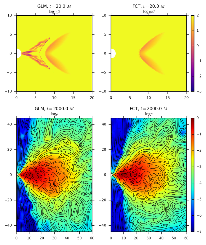
Figure 12: Magnetised torus: plasma $\beta$ at $t=20\,M$ (top) and density and magnetic field lines $t=2000\,M$ (bottom) using GLM (left) and FCT (right).

A qualitative difference can be seen even at early times of the simulation. The two upper panels of Fig. 12 show a snapshot of the simulation at $t=20\,M$ using both GLM and FCT. For GLM some of the magnetic field has diffused out of the original torus, magnetising the atmosphere. This artefact is visible for GLM from almost the beginning of the simulation ($t\approx 20\,M$), while for FCT it is minimal. Even though this particular artefact is not of crucial importance for the subsequent dynamics of the simulation, this points to a higher inclination of GLM to produce spurious magnetic field structures. At later times (bottom panels of Fig. 12), the most noticeable difference is the smaller amount of turbulent magnetic structures and the bigger plasma magnetisation inside the funnel in FCT, as compared to GLM. This latter difference indicates that the choice of technique to control $\nabla\cdot\boldsymbol{B}$ may have an effect on the possibility of jet formation in GRMHD simulations, although this specific effect was not extensively studied.

To summarise this small section on the comparison between both divergence-control techniques, we found from the three tests performed that FCT seems to be less diffusive than GLM, is able to preserve for a longer time a stationary solution, and seems to create less spurious structures in the magnetic field. However, it still has the inconvenient property that it is not possible to implement a cell-entered version of it whilst fully incorporating AMR. As mentioned previously, we are currently working on a staggered implementation adapted to AMR, and this will be described in a separate work.

4 Torus simulations

4.1 Initial conditions

We consider a hydrodynamic equilibrium torus threaded by a weak magnetic field loop. The particular equilibrium torus solution with constant angular momentum was first presented by Fishbone76 and Kozlowski1978 and is now a standard test for GRMHD simulations (see, e.g.,  Font02a, ; Zanotti03, ; Anton05, ; Rezzolla_book:2013, ; White2016, ). To facilitate cross-comparison, we set the initial conditions in the torus close to those adopted by Shiokawa2012 ; White2016 . Hence the spacetime is a Kerr BH with dimensionless spin parameter $a=0.9375$. The inner radius of the torus is set to $r_{\rm in}=6\,M$ and the density maximum is located at $r_{\rm max}=12\,M$, where radial and azimuthal positions refer to Boyer-Lindquist coordinates. With these choices, the orbital period of the torus at the density maximum becomes $T=247M$. We adopt an ideal gas EOS with an adiabatic index of $\hat{\gamma}=4/3$. A weak single magnetic field loop defined by the vector potential

$$A_{\phi}\propto{\rm max}(\rho/\rho_{\rm max}-0.2,0)\,,$$ (109)

is added to the stationary solution. The field strength is set such that $2p_{\rm max}/b^{2}_{\rm max}=100$, where global maxima of pressure $p_{\rm max}$ and magnetic field strength $b^{2}_{\rm max}$ do not necessarily coincide. In order to excite the MRI inside the torus, the thermal pressure is perturbed by $4\%$ white noise.

As with any fluid code, vacuum regions must be avoided and hence we apply floor values for the rest-mass density ($\rho_{\mathrm{fl}}=10^{-5}r^{-3/2}$) and the gas pressure ($p_{\mathrm{fl}}=1/3\times 10^{-7}\ r^{-5/2}$). In practice, for all cells which satisfy $\rho\leq\rho_{\mathrm{fl}}$ we set $\rho=\rho_{\mathrm{fl}}$, in addition if $p\leq p_{\mathrm{fl}}$, we set $p=p_{\mathrm{fl}}$.

The simulations are performed using horizon penetrating logarithmic KS coordinates (corresponding to our set of modified KS coordinates with $h=0$ and $R_{0}=0$). In the 2D cases, the simulation domain covers $r_{\rm KS}\in[0.96r_{\mathrm{h}},2500\,M]$ and $\theta\in[0,\pi]$, where $r_{\mathrm{h}}\simeq 1.35\,M$. In the 3D cases, we slightly excise the axial region $\theta\in[0.02\pi,0.98\pi]$ and adopt $\phi\in[0,2\pi]$. We set the boundary conditions in the horizon and at $r=2500\,M$ to zero gradient in primitive variables. The $\theta$-boundary is handled as follows: when the domain extends all the way to the poles (as in our 2D cases), we adopt “hard” boundary conditions, thus setting the flux through the pole manually to zero. For the excised cone in the 3D cases, we use reflecting “soft” boundary conditions on primitive variables.

The time-update is performed with a two-step predictor corrector based on the TVDLF fluxes and PPM reconstruction. Furthermore, we set the CFL number to 0.4 and use the FCT algorithm. Typically, the runs are stopped after an evolution for $t=5000\,M$, ensuring that no signal from the outflow boundaries can disturb the inner regions. To check convergence, we adopt the following resolutions: $N_{r}\times N_{\theta}\in\{256\times 128,512\times 256,1024\times 512\}$ in the 2D cases and $N_{r}\times N_{\theta}\times N_{\phi}\in\{128\times 64\times 64,192\times 96\times 96,256\times 128\times 128,384\times 192\times 192\}$ in the 3D runs. In the following, the runs are identified via their resolution in $\theta$-direction. For the purpose of validation, we ran the 2D cases also with the HARM3D code Noble2009 .

To facilitate a quantitative comparison, we report radial profiles of disk-averaged quantities similar to Shiokawa2012 ; White2016 ; Beckwith2008 . For a quantity $q(r,\theta,\phi,t)$, the shell average is defined as

$$\langle q(r,t)\rangle:=\frac{\int_{0}^{2\pi}\int_{\theta{\rm min}}^{\theta{\rm max}}q(r,\theta,\phi,t)\sqrt{-g}\,d\phi\,d\theta}{\int_{0}^{2\pi}\int_{\theta{\rm min}}^{\theta{\rm max}}\sqrt{-g}\,d\phi\,d\theta}\,,$$ (110)

which is then further averaged over a given time interval to yield $\langle q(r)\rangle$ (note that we omit the weighting with the density as done by Shiokawa2012 ; White2016 ). The limits $\theta_{\rm min}=\pi/3$, $\theta_{\rm max}=2\pi/3$ ensure that atmosphere material is not taken into account in the averaging. The time-evolution is monitored with the accretion rate $\dot{M}$ and the magnetic flux threading the horizon $\phi_{B}$

$$\dot{M} :=\int_{0}^{2\pi}\int_{0}^{\pi}\rho u^{r}\sqrt{-g}\,d\theta\,d\phi\,,$$ (111)

$$\phi_{B} :=\frac{1}{2}\int_{0}^{2\pi}\int_{0}^{\pi}|B^{r}|\sqrt{-g}\,d\theta\,d\phi\,,$$ (112)

where both quantities are evaluated at the outer horizon $r_{\mathrm{h}}$.

4.2 2D results

Figure 13 illustrates the qualitative time evolution of the torus by means of the rest-frame density $\rho$, plasma-$\beta$ and the magnetisation $\sigma=b^{2}/\rho$. After $t\simeq 300\,M$, the MRI-driven turbulence leads to accretion onto the central BH. The accretion rate and magnetic flux threading the BH then quickly saturate into a quasi-stationary state (see also Fig. 14). The accreted magnetic flux fills the polar regions and gives rise to a strongly magnetised funnel with densities and pressures dropping to their floor values. For the adopted floor values we hence obtain values of plasma-$\beta$ as low as $10^{-5}$ and magnetisations peaking at $\sigma\approx 10^{3}$ in the inner BH magnetosphere. These extreme values pose a stringent test for the robustness of the code and, consequently, the funnel region must be handled with the auxiliary inversion based on the entropy switch (see Sect. 2.10.2).

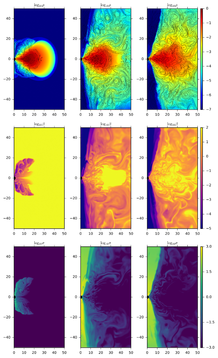
Figure 13: Evolution of the 2D magnetised torus with resolution $1024\times 512$ for times $t/M\in\{300,1000,2000\}$. We show logarithmic rest-frame density (top), logarithmic plasma $\beta$ (middle) and the logarithm of the magnetisation parameter $\sigma=b^{2}/\rho$ (bottom). Magnetic field lines are traced out in the first panel using black contour lines. One can clearly make out the development of the MRI and evacuation of a strongly magnetised funnel reaching values of $\beta<10^{-5}$ and $\sigma\approx 10^{3}$.

4.2.1 Comparison to HARM3D 

For validation purposes we simulated the same initial conditions with the HARM3D code. Wherever possible, we have made identical choices for the algorithm used in both codes, that is: PPM reconstruction, TVDLF Riemann solver and a two step time update. It is important to note that the outer radial boundary differs in both codes: while the HARM3D setup implements outflow boundary conditions at $r=50M$, in the BHAC runs the domain and radial grid is doubled in the logarithmic Kerr-Schild coordinates, yielding identical resolution in the region of interest. This ensures that no boundary effects compromise the BHAC simulation. Next to the boundary conditions, also the initial random perturbation varies in both codes which can amount to a slightly different dynamical evolution.

After verifying good agreement in the qualitative evolution, we quantify with both codes $\dot{M}$ and $\phi_{B}$ according to equations (111) and (112). The results are shown in Fig. 14. Onset-time of accretion, magnitude and overall behaviour are in excellent agreement, despite the chaotic nature of the turbulent flow. We also find the same trend with respect to the resolution-dependence of the results: upon doubling the resolution, the accretion rate $\langle\dot{M}\rangle$, averaged over $t\in[1000,2000]$, increases significantly by a factor of $1.908$ and $1.843$ for BHAC and HARM , respectively. For $\langle\phi_{B}\rangle$, the factors are $1.437$ and $1.484$. At a given resolution, the values for $\langle\dot{M}\rangle$ and $\langle\phi_{B}\rangle$ agree between the two codes within their standard deviations. Furthermore, we have verified that these same resolution variations are within the run-to-run deviations due to a different random number seed for the initial perturbation.

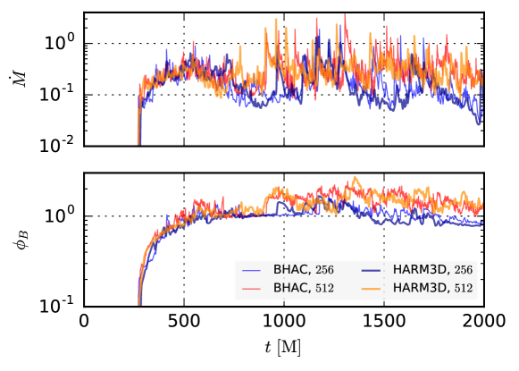
Figure 14: Accretion rates and horizon-penetrating magnetic flux in the 2D validation runs. We show two resolutions with each code: BHAC (blue, red) and HARM3D  (dark blue, orange). Despite the chaotic nature of the turbulent accretion both codes show very good qualitative and quantitative agreement.

Further validation is provided in Fig. 15 where disk-averaged profiles for the two highest resolution 2D runs are shown according to equation (110). The quantities of interest are the rest-frame density $\rho$, the dimensionless temperature $\Theta:=p/\rho c^{2}$, the magnitude of the fluid-frame magnetic field $|B|=\sqrt{b^{2}}$, thermal and magnetic pressures $P_{\rm gas}$, $P_{\rm mag}$ and the plasma-$\beta$. Again we set the averaging time $t\in[1000,2000]\,M$ with both codes. The agreement can be considered as very good, that is apart from a slightly higher magnetisation in HARM for $r\in[20,30]$, the differences of which are well within the $1\sigma$ standard deviation over the averaging time. Small systematic departures at the outer edge of the HARM domain are likely attributable to boundary effects.

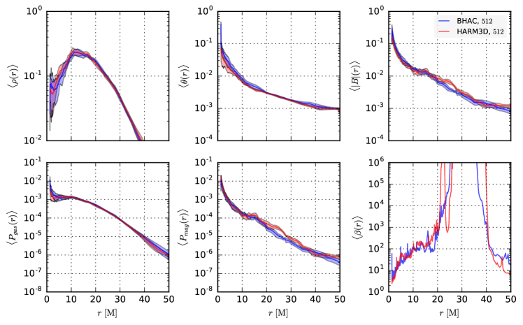
Figure 15: Disk-averaged quantities in the 2D validation runs. The blue curves are obtained with BHAC and the red curves with HARM3D in a two-dimensional setting. The shaded regions mark the $1\sigma$ standard deviation of the spatially-averaged snapshots (omitted for the highly fluctuating $\langle\beta\rangle$). Apart from a slightly higher magnetisation in HARM for $r\in[20,30]$, we find excellent agreement between both codes.

4.3 3D results

We now turn to the 3D runs performed with BHAC. The qualitative evolution of the high resolution run is illustrated in Fig. 16 showing rest-frame density and $b^{2}$ on the two slices $z=0$ and $y=0$. Overall, the evolution progresses in a similar manner to the 2D cases: MRI-driven accretion starts at $t\approx 300\,M$ and enters saturation at around $t\simeq 1000\,M$. Similar values for the magnetisation in the funnel region are also obtained. However, since the MRI cannot be sustained in axisymmetry as poloidal field cannot be re-generated via the ideal MHD induction equation (Cowling1933, ), we expect to see qualitative differences between the 2D and 3D cases at late times.

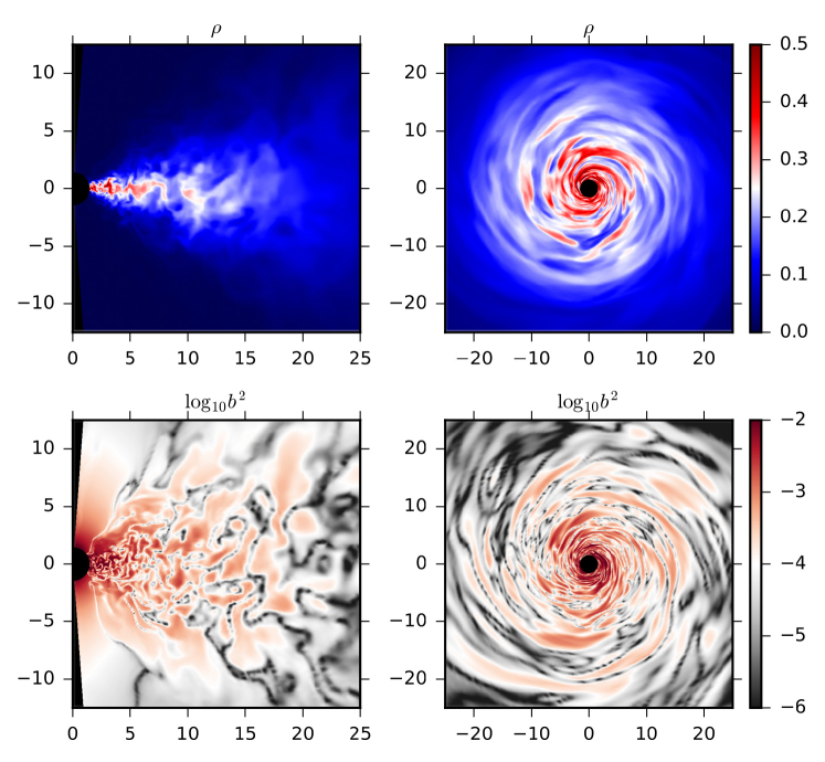
Figure 16: Fluid-frame density (top) and $\log_{10}b^{2}$ (bottom) for $t=3000\,M$ on the $y=0$ plane (left) and the $z=0$ plane (right) in the 3D magnetised torus run with resolution $384\times 192\times 192$.

Four different numerical resolutions were run which allows a first convergence analysis of the magnetised torus accretion scenario. Based on the convergence study, we can estimate which numerical resolutions are required for meaningful observational predictions derived from GRMHD simulations of this type.

Since we attempt to solve the set of dissipation-free ideal MHD equations, convergence in the strict sense cannot be achieved in the presence of a turbulent cascade (see also the discussion in SorathiaReynolds2012, ; HawleyRichers2013, ). Instead, given sufficient scale separation, one might hope to find convergence in quantities of interest like the disk averages and accretion rates. The convergence of various indicators in similar GRMHD torus simulations was addressed for example by Shiokawa2012 . The authors found signs for convergence in most quantifications when adopting a resolution of $192\times 192\times 128$, however no convergence was found in the correlation length of the magnetic field. Hence the question as to whether GRMHD torus simulations can be converged with the available computational power is still an open one.

From Figs. 17 and 18, it is clear that the resolution of the $N_{\theta}=64$ run is insufficient: a peculiar mini-torus is apparent in the disk-averaged density which diminishes with increasing resolution. Also the onset-time of accretion and the saturation values differ significantly between the $N_{\theta}=64$ run and its high-resolution counterparts. These differences diminish between the high-resolution runs and we can see signs of convergence in the accretion rate: increasing resolution from $N_{\theta}=128$ to $N_{\theta}=192$ appears to not have a strong effect on $\dot{M}$. Also the evolution of $\phi_{B}$ agrees quite well between $N_{\theta}=128$ and $N_{\theta}=192$. Hence the systematic resolution dependence of $\dot{M}$ and $\phi_{B}$ in the (even higher resolution) 2D simulations appears to be an artefact of the axisymmetry. It is also noteworthy that the variability amplitude of the accretion rate is reduced in the 3D cases. It appears that the superposition of uncorrelated accretion events distributed over the $\phi$-coordinate tends to smear out the sharp variability that results in the axisymmetric case.

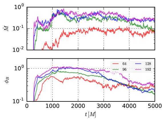
Figure 17: Accretion rates and horizon-penetrating magnetic flux in the 3D runs for varying numerical resolution. We show results from four different resolutions labeled according to the number of cells in $\theta$-direction.

Although the simulations were run until $t=5000\,M$, in order to enable comparison with the 2D simulations, we deliberately set the averaging time to $t\in[1000\,M,2000\,M]$. Figure 18 shows that as the resolution is increased, the disk-averaged 3D data approaches the much higher resolution 2D results shown in Fig. 15, indicating that the dynamics are dominated by the axisymmetric MRI modes at early times. When the resolution is increased from $N_{\theta}=128$ to $N_{\theta}=192$, the disk-averaged profiles generally agree within their standard deviations, although we observe a continuing trend towards higher gas pressures and magnetic pressures in the outer regions $r\in[30M,50M]$. The overall computational cost quickly becomes significant: for the $N_{\theta}=128$ simulation we spent $100\,K$ CPU hours on the Iboga cluster equipped with Intel(R) Xeon(R) E5-2640 v4 processors. As the runtime scales with resolution according to $N_{\theta}^{4}$, doubling resolution would cost a considerable $1.6\,M$ CPU hours.

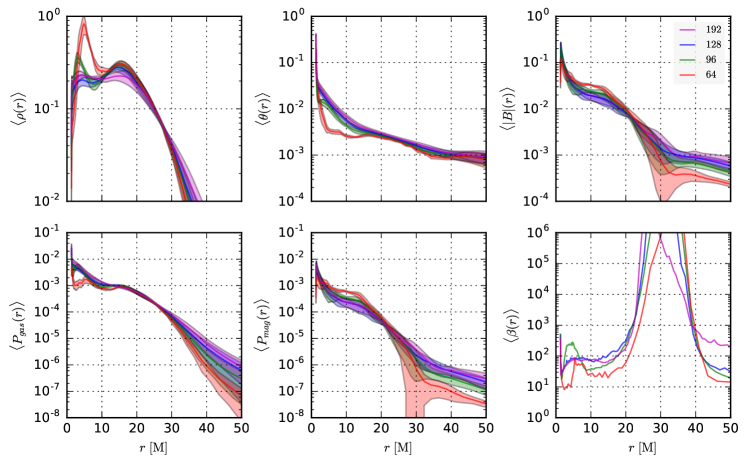
Figure 18: Disk-averaged quantities in the 3D runs for varying numerical resolution. The shaded regions mark the $1\sigma$ standard deviation of the spatially-averaged snapshots as in Fig. 15.

4.4 Effect of AMR

In order to investigate the effect of the AMR treatment, we have performed a 2D AMR-GRMHD simulation of the torus setup. It is clear that whether a simulation can benefit from adaptive mesh refinement is very much dependent on the physical scenario under investigation. For example, in the hydrodynamic simulations of recoiling BHs due to Meliani2017 , refinement on the spiral shock was demonstrated to yield significant speedups at a comparable quality of solution. This is understandable as the numerical error is dominated by the shock hypersurface. In the turbulent accretion problem, whether automated mesh refinement yields any benefits is not clear.

The initial conditions for this test are the same as those used in Sect. 4.1. However, due to the limitation of current AMR treatment, we resort to the GLM divergence cleaning method. Three refinement levels are used and refinement is triggered by the error estimator due to Loehner87 with the tolerance set to $\epsilon_{\mathrm{t}}=0.1$ (see Sect. 2.11). The numerical resolution in the base level is set to $N_{r}\times N_{\theta}=128\times 128$. To test the validity and efficiency, we also perform the same simulation in a uniform grid with resolution of $N_{r}\times N_{\theta}=512\times 512$ which corresponds to the resolution on the highest AMR level.

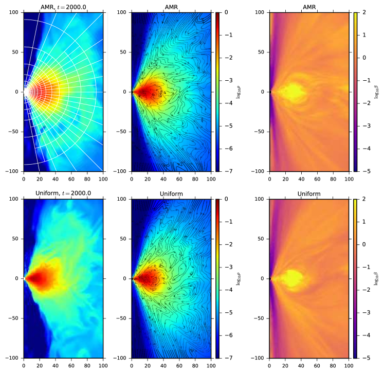
Figure 19: 2D logarithmic density at $t=2000\,M$ (left), averaged density (middle), and averaged plasma beta (right) of the 2D magnetised torus with three-levels AMR (top panels) and uniform resolution $512\times 512$ (bottom panels). Magnetic field lines are traced out in the middle panels using black contour lines. The averaged quantities are calculated in the time interval $t\in[1000\,M,2000\,M]$. AMR blocks containing $16^{2}$ cells are indicated in the upper left panel.

Figure 19 shows the densities at $t=2000\,M$ as well as the time-averaged density and plasma beta for the AMR and uniform cases. The averaged quantities are calculated in the time interval of $t\in[1000\,M,2000\,M]$. The overall behaviour is quite similar in both cases. Naturally, differences are seen in the turbulent structure in the torus and wind region for a single snapshot. However, in terms of averaged quantities, the difference becomes marginal. In order to better quantify the difference between the AMR and uniform runs, the mass accretion rate and horizon penetrating magnetic flux are shown in Fig. 20. These quantities exhibit a similar behaviour in both cases. In particular, the difference between the AMR run and the uniform run is smaller than the one from different resolution uniform runs and compatible with the run-to-run variation due to a different random number seed (cf. Sect. 4.2). This is unsurprising since the error estimator triggers refinement of the innermost torus region to the highest level of AMR during most of the simulation time. The development of small scale turbulence by the MRI is clearly captured and it leads to similar mass accretion onto the BH.

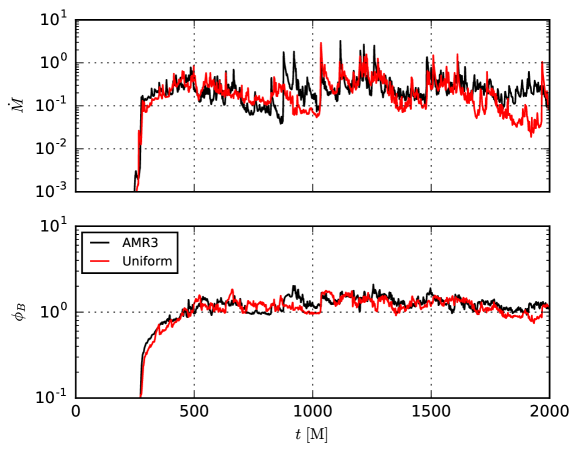
Figure 20: Accretion rates and horizon penetrating magnetic flux of the 2D magnetised torus with three levels of AMR (black) and uniform resolution $512\times 512$ (red).

Table 5: CPU hours (CPUH) spent by the simulations of the 2D magnetised torus at uniform resolution and fraction of that time spent by the equivalent AMR runs up to $t=2000\,M$.

Grid size	CPU time	Equiv. AMR
$(N_{r}\times N_{\theta})$	uniform	time fraction
	[CPUH]	[$\epsilon_{\mathrm{t}}=0.1$]
$512\times 512$	674.0	0.643

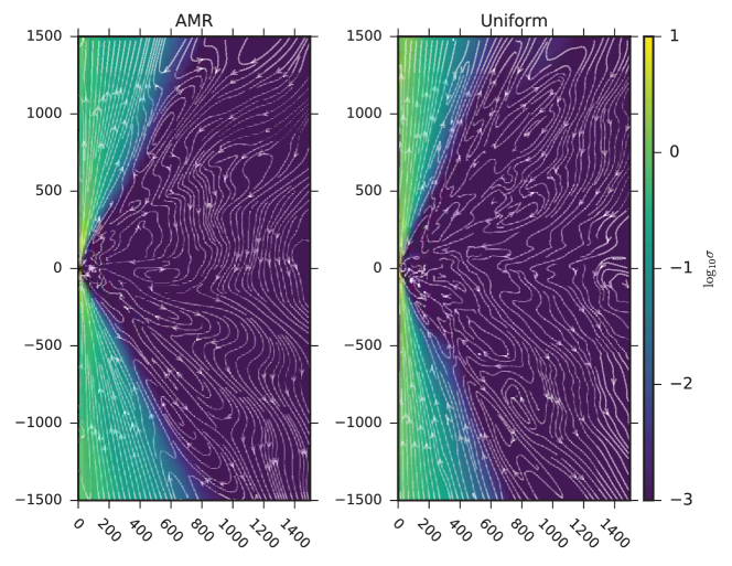
Figure 21: 2D logarithmic averaged magnetisation of the magnetised torus with three levels of AMR (left) and uniform resolution $512\times 512$ (right). Magnetic field lines are traced out by white contour-lines. The averaged quantities are calculated in the time interval of $t\in[6000\,M,10000\,M]$.

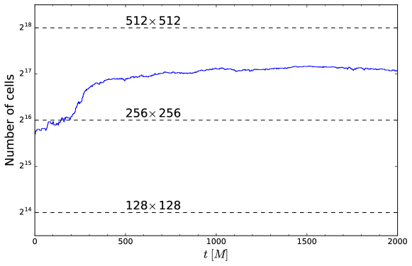
Figure 22: Number of cells as a function of time for the AMR simulation. The dotted lines show the resolution of uniform grids equivalent to each of the three AMR levels.

One of the important merits of using AMR is the possibility to resolve small and large scale dynamics simultaneously with lower computational cost than uniform grids. Figure 21 shows the large scale structure of the averaged magnetisation after $10000\,M$ of simulation time. The averaged quantities are calculated in the time interval $t\in[6000\,M,10000\,M]$. In order to allow the large-scale magnetic field structure to settle down, we average over a later simulation time compared to the previous non-AMR cases. From the figure the collimation angle and magnetisation of the highly magnetised funnel in the AMR case are slightly wider than those in uniform case but the large-scale global structure is very similar in both cases.

A comparison of the computational time for a uniform resolution with $512^{2}$ and the equivalent AMR run (three-level AMR) is shown in Table 5. It is encouraging that even in the naive three-level AMR simulation we obtain qualitatively similar results comparable to the high resolution uniform run, but with having spent only $64\%$ of the computational time of the uniform run. Figure 22 shows the evolution of the total number of cells during the simulations of AMR cases. Initially less than $2^{16}$ cells are used even when we use three AMR levels, which is a similar number of cells as the uniform grid case with $256\times 256$. When the simulation starts, the total cell number increases rapidly due to development of turbulence in the torus which is triggering higher refinement. We note that the total number of cells is still half of the total number of cells in the corresponding high-resolution uniform grid simulation ($512\times 512$), thus resulting in a direct reduction of computational cost. With increasing dynamic range, we expect the advantages of AMR to increase significantly, rendering it a useful tool for simulations involving structures spanning multiple scales. We leave a more detailed discussion on the effect of the AMR refinement strategy and various divergence-control methods to a future paper.

5 Radiation post-processing

In order to compute synthetic observable images of the BH shadow and surrounding accretion flow it is necessary to perform general-relativistic ray-tracing and GRRT post-processing (see, e.g.,  Fuerst2004, ; Vincent2011, ; Younsi2012, ; Younsi2015, ; Chan2015, ; Dexter2016, ; Pu2016, ; Younsi2016, ). In this article the GRRT code BHOSS (Black Hole Observations in Stationary Spacetimes) Younsi2017 is used to perform these calculations. From BHAC, GRMHD simulation data are produced which are subsequently used as input for BHOSS. Although BHAC has full AMR capabilities, for the GRRT it is most expedient to output GRMHD data that has been re-gridded to a uniform grid.

Since these calculations are performed in post-processing, the effects of radiation forces acting on the plasma during its magnetohydrodynamical evolution are not included. Additionally, the fast-light approximation has also been adopted in this study, i.e., it is assumed that the light-crossing timescale is shorter than the dynamical timescale of the GRMHD simulation and the dynamical evolution of the GRMHD simulation as light rays propagate through it is not considered. Such calculations are considered in an upcoming article Younsi2017 .

Several different coordinate representations of the Kerr metric are implemented in BHOSS, including Boyer-Lindquist (BL), Logarithmic BL, Cartesian BL, Kerr-Schild (KS), Logarithmic KS, Modified KS and Cartesian KS. All GRMHD simulation data used in this study are specified in Logarithmic KS coordinates. Although BHOSS can switch between all coordinate systems on the fly, it is most straightforward to perform the GRRT calculations in the same coordinate system as the GRMHD data, only adaptively switching to e.g., Cartesian KS when near the polar region. This avoids the need to transform between coordinate systems at every point along every ray in the GRMHD data interpolation, saving computational time.

5.1 Radiative transfer equation

Electromagnetic radiation is described by null geodesics of the background spacetime (in this case Kerr), and these are calculated in BHOSS using a Runge-Kutta-Fehlberg integrator with fourth order adaptive step sizing and 5th order error control. Any spacetime metric may be considered in BHOSS, as long as the contravariant or covariant metric tensor components are specified, even if they are only tabulated on a grid. For the calculations presented in this article the Kerr spacetime is written algebraically and in closed-form.

The observer is calculated by constructing a local orthonormal tetrad using trial basis vectors. These basis vectors are then orthonormalized using the metric tensor through a modified Gram-Schmidt procedure. The initial conditions of each ray for the coordinate system under consideration are then calculated and the geodesics are integrated backwards in time from the observer, until they either: (i) escape to infinity (exit the computational domain), (ii) are captured by the BH, or (iii) are effectively absorbed by the accretion flow.

In order to perform these calculations the GRRT equation is integrated in parallel with the geodesic equations of motion of each ray. Written in covariant form, the (unpolarized) GRRT equation, in the absence of scattering, may be written (Younsi2012, ) as

$$\frac{d\mathcal{I}}{d\lambda}=-k_{\mu}u^{\mu}\left(-\alpha_{\nu,0}\,\mathcal{I}+\frac{j_{\nu,0}}{\nu_{0}^{3}}\right)\,,$$ (113)

where $\mathcal{I}:=I_{\nu}/\nu^{3}$ is the Lorentz-invariant intensity, $I_{\nu}$ is the specific intensity, $\nu$ is the frequency of radiation, $\alpha_{\nu,0}$ is the specific absorption coefficient and $j_{\nu,0}$ is the specific emission coefficient. The subscript “$\nu$” denotes evaluation of a quantity at a specific frequency, $\nu$, and a subscript “$0$” denotes evaluation of a quantity in the local fluid rest frame. The terms $k_{\mu}$ and $u^{\mu}$ are the photon $4$-momentum and the fluid $4$-velocity of the emitting medium, respectively. The former is calculated from the geodesic integration and the latter is determined from the GRMHD simulation data. The affine parameter is denoted by $\lambda$.

By introducing the optical depth along the ray

$$\tau_{\nu}\left(\lambda\right)=-\int_{\lambda_{0}}^{\lambda}\ \!\alpha_{\nu,0}\left(\lambda^{\prime}\right)k_{\mu}u^{\mu}\,d\lambda^{\prime}\,,$$ (114)

together with the Lorentz-invariant emission coefficient $\left(\eta=j_{\nu}/\nu^{2}\right)$ and Lorentz-invariant absorption coefficient $\left(\chi=\nu\alpha_{\nu}\right)$, the GRRT equation (113) may be rewritten as

$$\frac{d\mathcal{I}}{d\tau_{\nu}}=-\mathcal{I}+\frac{\eta}{\chi}\,.$$ (115)

Following Younsi2012 , equation (115) may be reduced to two differential equations

$$\gamma\frac{d\tau_{\nu}}{d\lambda} = \alpha_{\nu,0}\,,$$ (116)

$$\gamma\frac{d\mathcal{I}}{d\lambda} = \frac{j_{\nu,0}}{\nu_{0}^{3}}\ \!\mathrm{exp}\left(-\tau_{\nu}\right)\,,$$ (117)

where

$$\gamma=\frac{\nu}{\nu_{0}}=\frac{\left(k_{\alpha}u^{\alpha}\right)_{\mathrm{obs}}}{\left(k_{\beta}u^{\beta}\right)_{0}}\,,$$ (118)

is the relative energy shift between the observer (“obs”) and the emitting fluid element. Integrating the GRRT equation in terms of the optical depth in the manner presented provides two major advantages. Firstly, the calculation of the geodesic and of the radiative transfer equation may be performed simultaneously, rather than having to calculate the entire geodesic, store it in memory, and then perform the radiative transfer afterwards. Secondly, by integrating in terms of the optical depth we may specify a threshold value (typically of order unity) whereby the geodesic integration is terminated when encountering optically thick media exceeding this threshold. The combination of these two methods saves significant computational time and expense.

5.2 BHOSS-simulated emission from Sgr A*

Having in mind the upcoming radio observations of the BH candidate Sgr A* at the Galactic Centre, the following discussion presents synthetic images of Sgr A*. The GRMHD simulations evolve a single fluid (of ions) and are scale-free in length and mass. Consequently a scaling must be applied before performing GRRT calculations. Within BHOSS this means specifying the BH mass, which sets the length and time scales, and specifying either the mass accretion rate or an electron density scale, which scales the gas density, temperature and magnetic field strength to that of a radiating electron.

Since the GRMHD simulation is of a single fluid, it is necessary to adopt a prescription for the local electron temperature and rest-mass density. Several such prescriptions exist, some which scale using the mass accretion rate (see, e.g.,  Moscibrodzka2009, ; Moscibrodzka2014, ; Dexter2010, ), scale using density to determine the electron number density and physical accretion rate (see, e.g.,  Chan2015, ; Chan2015b, ), and some by employing a time-dependent smoothing model of the mass accretion rate (see, e.g.,  Shiokawa2012, ).

The dimensionless proton temperature, $\Theta_{\mathrm{p}}$, is defined as

$$\Theta_{\mathrm{p}}:=\frac{k_{\mathrm{B}}T_{\mathrm{p}}}{m_{\mathrm{p}}c^{2}}\,,$$ (119)

where $k_{\mathrm{B}}$ is the Boltzmann constant, $T_{\mathrm{p}}$ is the geometrical (i.e., in physical units) proton temperature and $m_{\mathrm{p}}$ is the proton mass. This is then calculated from the GRMHD simulation density ($\rho$) and pressure ($p$) as

$$\Theta_{\mathrm{p}}=\frac{3p}{\rho}\,,$$ (120)

where the fact that the equation of state is ideal and that $\hat{\gamma}=4/3$ has been assumed. The magnetic field strength in geometrical units, $B_{\mathrm{geo}}$, is readily obtained from the code magnetic field strength $B=\sqrt{b_{\mu}b^{\mu}}$ as

$$B_{\mathrm{geo}}=c\left(\frac{\rho_{\mathrm{geo}}}{\rho}\right)^{1/2}B\,.$$ (121)

What remains is to specify $T_{\mathrm{e}}$ (or $\Theta_{\mathrm{e}}:=k_{\mathrm{B}}T_{\mathrm{e}}/m_{\mathrm{e}}c^{2}$) and $\rho_{\mathrm{geo}}$. For simplicity we adopt the prescription of Moscibrodzka2009 , wherein $T_{\mathrm{p}}/T_{\mathrm{e}}$ is assumed to be a fixed ratio. Whilst such an approximation is rather crude, to zeroth order the protons and electrons may be assumed to be coupled in this way. To scale the electron number density we adopt the method of Chan2015 , assuming a density scale typically of order $10^{7}~{}\mathrm{cm}^{-3}$. A somewhat more sophisticated approach is to employ a thresholding of the fluid plasma beta where, when the local plasma beta exceeds some threshold the electrons and protons are coupled as previously mentioned (disk region), but when not exceeded (typically in the funnel region) the electron temperature is assumed to be constant (Moscibrodzka2014, ; Moscibrodzka2016, ; Chan2015, ). Since plasma beta is found to decrease with resolution (Shiokawa2012, ) and in this paper we seek only to demonstrate the convergence of our simulated shadow images obtained from the GRMHD data in regions where the density is non-negligible, we adopt the former model.

For the plasma emissivity we use the approximate formula for thermal magnetobremsstrahlung (Leung2011, ), which is given by

$$j_{\nu}=\left(\frac{\sqrt{2}\pi e^{2}}{3c}\right)n_{\mathrm{e}}\frac{\nu_{\mathrm{s}}}{K_{2}\left(\Theta_{\mathrm{e}}^{-1}\right)}\left(X^{1/2}+2^{11/12}X^{1/6}\right)^{2}\exp\left(-X^{1/3}\right)\,,$$ (122)

where $e$ is the electron charge, $n_{\mathrm{e}}$ the electron number density, and

$$X := \frac{\nu}{\nu_{\mathrm{s}}}\,,$$ (123)

$$\nu_{\mathrm{s}} = \left(\frac{e}{9\pi m_{\mathrm{e}}c}\right)B\Theta_{\mathrm{e}}^{2}\sin\vartheta\,,$$ (124)

and $\vartheta$ is the pitch angle of the photon with respect to the magnetic field. The absorption coefficient is readily obtained from Kirchoff’s law.

Each image is generated using a uniform grid of $1000\times 1000$ rays, sampling 60 uniformly logarithmically spaced frequency bins between $10^{9}$ Hz and $10^{15}$ Hz. All panels depict the observed image as seen at an observational frequency of $230~{}$GHz, i.e. the frequency at which the EHT will image Sgr A*. This resolution is chosen because the integrated flux over the entire ray-traced image is convergent: doubling the resolution from $500\times 500$ to $1000\times 1000$ yields an increase of $0.17\%$, and from $1000\times 1000$ to $2000\times 2000$ an increase of $0.09\%$.

In practical GRRT calculations only simulation data which has already reached a quasi-steady state, typically $t>2000\,M$, is used. In this study we focus on the observational appearance of the accretion flow and BH shadow image. The detailed discussion of the spectrum, variability and plasma models warrants a separate study.

5.3 Comparison of images

A natural and important question arises from GRRT calculations of BH shadows: do ray-traced images of GRMHD simulation data converge as the resolution of the GRMHD simulation is increased? The existence of an optimal resolution, beyond which differences in images are small, implies that one can save additional computational time and expense by running the simulation at this optimal resolution. It would also imply that the GRMHD data satisfactorily capture the small-scale structure, turbulence and variations of the accretion flow. As such, it is informative to investigate the convergence of BH shadow images obtained from GRMHD simulation data of differing resolutions, both quantitatively and qualitatively.

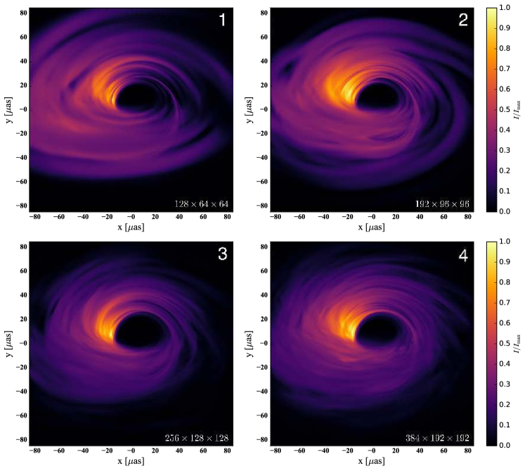
Figure 23: Snapshot images of 3D GRMHD simulation data with parameters chosen to mimic the emission from Sgr A*. The resolution of the simulation data is indicated in the bottom-right corner of each panel and discussed in the text.

To address this question we first generate a series of four snapshot images at $t=2500\,M$ of the the accretion flow and BH shadow from GRMHD simulation data. The resolution of these data are $2\mathcal{N}\times\mathcal{N}\times\mathcal{N}$ in $(r,\theta,\phi)$, i.e., twice as much resolution in the radial direction compared to the zenith and azimuthal directions. The images depicted in Fig. 23 correspond to $\mathcal{N}=64$, $96$, $128$ and $192$ respectively. Here, the proton to electron temperature ratio was chosen as $T_{\mathrm{p}}/T_{\mathrm{e}}=3$ (similar to Moscibrodzka2009 ; Moscibrodzka2014 ), the electron number density scaling as $5\times 10^{7}~{}\mathrm{cm}^{-3}$, the BH mass is set to $4.5\times 10^{6}~{}M_{\odot}$, the source distance is $8.4\times 10^{3}~{}\mathrm{pc}$, the dimensionless BH spin parameter $0.9375$ and the observer inclination angle with respect to the BH spin axis is $60^{\circ}$.

A direct consequence of increasing the resolution of the GRMHD data is resolving the fine-scale turbulent structure of the accretion flow. The characteristic dark shadow delineating the BH shadow can be clearly seen in all images. As the resolution of the GRMHD data is increased, the images become less diffuse. It is difficult with the naked eye to draw firm physical conclusions, and so in the following we perform a quantitative pixel-by-pixel analysis.

With these snapshot images we may perform a quantitative measure of the difference between any two images through introducing the (normalised) cross-correlation. For two given two-dimensional arrays $f(x,y)$ and $g(x,y)$ (i.e., 2D images), a measure of similarity or difference may be calculated through the cross-correlation $\mathcal{C}$, where $\mathcal{C}\in[-1,1]$. The normalised cross-correlation is defined as

$$\mathcal{C}:=\mathcal{C}_{{}_{i,j}}:=\frac{1}{N\sigma_{f}\sigma_{g}}\sum\limits_{x,y}\left\{\left[f(x,y)-\mu_{f}\right]\left[g(x,y)-\mu_{g}\right]\right\}\,,$$ (125)

where $\mu_{f},\ \sigma_{f}$ and $\mu_{g},\ \sigma_{g}$ correspond to the mean and standard deviation of $f$ and $g$ respectively, and $N$ is equal to the size of either $f$ or $g$. In the examples considered here the images are all of equal size and dimension, so $N=N_{f}=N_{g}$. Equation (125) may be interpreted as the inner product between two data arrays, with the value of $\mathcal{C}$ expressing the degree to which the data are aligned with respect to each other. When $\mathcal{C}=1$ the data are identical, save for a multiplicative constant, when $\mathcal{C}=0$ the data are completely uncorrelated, and when $\mathcal{C}<0$ the data are negatively correlated.

Each image pixel has an intensity value represented as a single greyscale value between zero and one. Given the relative intensity data of two different images, Equation (125) is then employed to determine the normalised cross-correlation between the two images. This procedure applied to the panels in Fig. (23) yields the following symmetric matrix of cross-correlation values between the images

$$\mathcal{C}_{i,j}=\left(\begin{array}[]{cccc}1&0.839495&0.809205&0.856958\\ -&1&0.867578&0.917560\\ -&-&1&0.948544\\ -&-&-&1\\ \end{array}\right)\,.$$ (126)

Indices $i$ and $j$, where $\left(i,j\right)=(1,4)$, denote the images being cross-correlated.

The rightmost column of equation (126) denotes the cross-correlation values, $\mathcal{C}_{i,4}$, in descending order between images, i.e., the cross-correlation of image 4 with images 1, 2, 3 and 4 respectively. Since $\mathcal{C}_{i+1,4}>\mathcal{C}_{i,4}$ it is clear that the similarity between images increases as the resolution of the GRMHD simulation is increased. Similarly, for image 3 it is found that $\mathcal{C}_{i+1,3}>\mathcal{C}_{i,3}$. Finally, it also follows that $\mathcal{C}_{3,4}>\mathcal{C}_{2,3}>\mathcal{C}_{1,2}$, i.e., the correlation between successive pairs of images increases with increasing resolution, demonstrating the convergence of the GRMHD simulations with increasing grid resolution. Whilst the lowest resolution of $128\times 64\times 64$ is certainly insufficient, both difference images and cross-correlation measures indicate that a resolution of $256\times 128\times 128$ is sufficient and represents a good compromise.

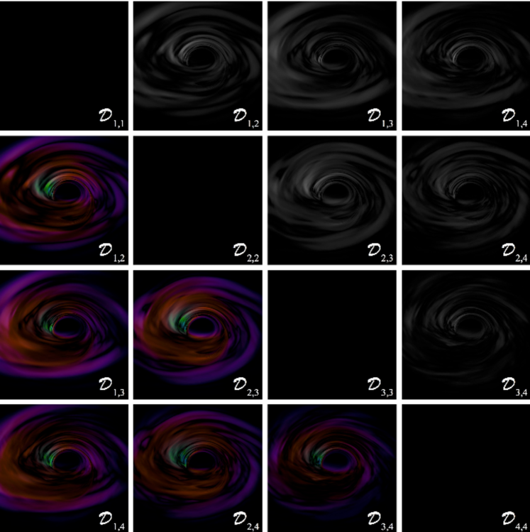
Figure 24: Matrix of image differences $\mathcal{D}_{i,j}$ of the four panels in Fig. 23. Upper diagonal panels are greyscale differences. Lower diagonal panels are identical to corresponding upper diagonal panels but with differences illustrated with RGB pixel values. Black panels correspond to $\mathcal{D}_{i,i}$, i.e., trivially the difference between an image and itself.

6 Conclusions and outlook

We have described the capabilities of BHAC, a new multidimensional general-relativistic magnetohydrodynamics code developed to perform hydrodynamical and MHD simulations of accretion flows onto compact objects in arbitrary stationary spacetimes exploiting the numerous advantages of AMR techniques. The code has been tested with several one-, two- and three- dimensional scenarios in special-relativistic and general-relativistic MHD regimes. For validation, GRMHD simulations of MRI unstable tori have been compared with another well-known and tested GRMHD code, the HARM3D code. BHAC shows very good agreement with the HARM3D results, both qualitatively and quantitatively. As a first demonstration of the AMR capabilities in multi-scale simulations, we performed the magnetized-torus accretion test with and without AMR. Despite the latter intrinsically implies an overhead of $\sim 10\%$, the AMR runtime amounted to $65\%$ of that relative to the uniform grid, simply as a result of the more economical use of grid cells in the block based AMR. At the same time, the AMR results agree very well with the more expensive uniform-grid results. With increasing dynamic range, we expect the advantages of AMR to increase even more significantly, rendering it a useful tool for simulations involving structures of multiple physical scales.

Currently, two methods controlling the divergence of the magnetic field are available in BHAC and we compared them in three test problems. Although solutions obtained with the cell-centered flux-interpolated constrained transport (FCT) algorithm and the divergence cleaning scheme (GLM) yield the same (correct) physical behaviour in the case of weak magnetic fields, FCT performs considerably better in the presence of strong magnetic fields. In particular, FCT is less diffusive than GLM, is able to preserve a stationary solution, and it creates less spurious structures in the magnetic field. For example, the use of GLM in the case of accretion scenarios with strong magnetic fields leads to worrisome artefacts in the highly magnetised funnel region. The development of a constrained transport scheme compatible with AMR is ongoing and will be presented in a separate work Olivares2017 .

The EHTC and its European contribution, the BlackHoleCam project (Goddi2016, ), aim at obtaining horizon-scale radio images of the BH candidate at the Galactic Center. In anticipation of these results, we have used the 3D GRMHD simulations as input for GRRT calculations with the newly developed BHOSS code (Younsi2017, ). We found that the intensity maps resulting from different resolution GRMHD simulations agree very well, even when comparing snapshot data that was not time averaged. In particular, the normalised cross-correlation between images achieves up to $94.8\%$ similarity between the two highest resolution runs. Furthermore, the agreement between two images converges as the resolution of the GRMHD simulation is increased. Based on this comparison, we find that moderate grid resolutions of $256\times 128\times 128$ (corresponding to physical resolutions of $\Delta r_{\rm KS}\times\Delta\theta_{\rm KS}\times\Delta\phi_{\rm KS}=0.04M\times 0.024{\rm rad}\times 0.05{\rm rad}$ at the horizon) yield sufficiently converged intensity maps. Given the large and likely degenerate parameter space and the uncertainty in modelling of the electron distribution, this result is encouraging, as it demonstrates that the predicted synthetic image is quite robust against the ever-present time variability, but also against the impact that the grid resolution of the GRMHD simulations might have. In addition, independent information on the spatial orientation and magnitude of the spin, such as the one that could be deduced from the dynamics of a pulsar near Sgr A* Psaltis2016 , would greatly reduce the space of degenerate solutions and further increase the robustness of the predictions that BHAC will provide in terms of synthetic images.

Finally, we have demonstrated the excellent flexibility of BHAC with a variety of different astrophysical scenarios that are ongoing and will be published shortly. These include: oscillating hydrodynamical equilibrium tori for the modelling of quasi-periodic oscillations deAvellar2017 , episodic jet formation Porth2017 and magnetised tori orbiting non-rotating dilaton BHs Mizuno2017 .

Appendix A Evolution of the scalar $\phi$

To obtain the evolution equation for $\phi$ in the augmented Faraday’s law, we project (58) onto the Eulerian observer by contracting with $-n_{\mu}$ as

$$-\nabla_{\nu}(^{*}\!F^{\mu\nu}n_{\mu}-\phi n^{\nu}) =-\kappa\phi-(^{*}\!F^{\mu\nu}-\phi g^{\mu\nu})\nabla_{\nu}n_{\mu}$$ (127)

$$\Rightarrow\nabla_{\nu}B^{\nu}+\nabla_{\nu}\phi n^{\nu} =-\kappa\phi-(^{*}\!F^{\mu\nu}-\phi g^{\mu\nu})\nabla_{\nu}n_{\mu}$$ (128)

$$\Rightarrow(-g)^{-1/2}\partial_{i}[\gamma^{1/2}\alpha B^{i}]+\nabla_{\nu}\phi n^{\nu} =-\kappa\phi-(^{*}\!F^{\mu\nu}-\phi g^{\mu\nu})\nabla_{\nu}n_{\mu}\,,$$ (129)

where we used $B^{\nu}=-n_{\mu}\,^{*}\!F^{\mu\nu}$. Using the definition of extrinsic curvature $K_{\mu\nu}:=-\gamma^{\lambda}_{\mu}\nabla_{\lambda}n_{\nu}$, we can write (Eq. (7.62) in Rezzolla_book:2013, )

$$\nabla_{\nu}n_{\mu}=-n_{\nu}a_{\mu}-K_{\mu\nu}\,,$$ (130)

where we used the “acceleration” of the Eulerian observer $a_{\mu}:=n^{\lambda}\nabla_{\lambda}n_{\mu}$ which satisfies $n^{\mu}a_{\mu}=0$. With the identity $a_{i}=\alpha^{-1}\partial_{i}\alpha$ (York79, ) and exploiting the symmetries of ${}^{*}\!F^{\mu\nu}$ and $K_{\mu\nu}$, is straightforward to show that

$$(\gamma)^{-1/2}\partial_{i}[(\gamma)^{1/2}\alpha B^{i}]+\alpha F^{*\mu\nu}\nabla_{\nu}n_{\mu}=(\gamma)^{-1/2}\partial_{i}[(\gamma)^{1/2}\alpha B^{i}]-B^{i}\partial_{i}\alpha\,.$$ (131)

Hence it follows that

$$\begin{split}\partial_{t}(\sqrt{\gamma}\phi)+\partial_{i}[\sqrt{\gamma}(\alpha B^{i}-\phi\beta^{i})]=&-\alpha\gamma^{1/2}\kappa\phi+\alpha\gamma^{1/2}\phi g^{\mu\nu}\nabla_{\nu}n_{\mu}\\ &+\gamma^{1/2}B^{i}\partial_{i}\alpha\,.\end{split}$$ (132)

Using again Eq. (130), the source term $\mathcal{S}:=\sqrt{\gamma}\alpha\phi g^{\mu\nu}\nabla_{\nu}n_{\mu}$ can be rewritten as

$$\mathcal{S}=-\sqrt{\gamma}\alpha\phi g^{\mu\nu}K_{\mu\nu}\,,$$ (133)

where the first term drops out due to the orthogonality $n^{\mu}a_{\mu}=0$. For a symmetric tensor $S^{\mu\nu}$, we have

$$\alpha S^{\mu\nu}K_{\mu\nu}=\alpha S^{ij}K_{ij}=S^{i}_{j}\partial_{i}\beta^{j}+\frac{1}{2}S^{ij}\beta^{k}\partial_{k}\gamma_{ij}\,.$$ (134)

This follows from the relation $\Gamma^{0}_{ij}=-K_{ij}\alpha^{-1}$ where $\Gamma^{0}_{ij}$ are elements of the 4-Christoffel symbols (see e.g., (B.9) of Alcubierre:2008, ). Thus

$$\mathcal{S} =-\sqrt{\gamma}\phi(\partial_{i}\beta^{i}+\frac{1}{2}\gamma^{ij}\beta^{k}\partial_{k}\gamma_{ij})$$ (135)

$$=-\sqrt{\gamma}\phi\partial_{i}\beta^{i}-\sqrt{\gamma}\phi\frac{1}{2}\gamma^{ij}\beta^{k}\partial_{k}\gamma_{ij}\,.$$ (136)

Appendix B Modified Faraday’s law

The augmented Faraday’s law follows from the $j$-component of (58) as

$$\nabla_{\nu}(^{*}\!F^{j\nu}-\phi g^{j\nu})=\kappa\phi\beta^{j}/\alpha$$ (137)

$$\Rightarrow (-g)^{-1/2}\left\{\partial_{t}[\sqrt{\gamma}(-B^{j})]+\partial_{i}\left[\sqrt{\gamma}\left(\mathcal{V}^{j}B^{i}-\mathcal{V}^{i}B^{j}\right)\right]\right\}+g^{j\lambda}\partial_{\lambda}(-\phi)=\kappa\phi\beta^{j}/\alpha$$ (138)

$$\Rightarrow \partial_{t}\left(\sqrt{\gamma}B^{j}\right)+\partial_{i}\left[\sqrt{\gamma}\left(\mathcal{V}^{i}B^{j}-\mathcal{V}^{j}B^{i}\right)\right]+\sqrt{\gamma}\alpha g^{j\lambda}\partial_{\lambda}\phi=-\kappa\phi\sqrt{\gamma}\beta^{j}$$ (139)

$$\Rightarrow \partial_{t}\left(\sqrt{\gamma}B^{j}\right)+\partial_{i}\left[\sqrt{\gamma}\left(\mathcal{V}^{i}B^{j}-\mathcal{V}^{j}B^{i}\right)\right]+\frac{\beta^{j}}{\alpha}\partial_{t}(\sqrt{\gamma}\phi)+\sqrt{\gamma}\alpha\gamma^{ji}\partial_{i}\phi$$

$$\hskip 170.71652pt-\sqrt{\gamma}\frac{\beta^{i}\beta^{j}}{\alpha}\partial_{i}\phi=-\sqrt{\gamma}\kappa\phi\beta^{j}\,.$$ (140)

We see that apart from the gradient $\phi$-term, we obtain another term that involves the time-derivative of $(\sqrt{\gamma}\phi)$. Hence we need to plug in Equation (59). We rewrite the term ${\beta^{j}}\partial_{t}(\sqrt{\gamma}\phi)/{\alpha}$ simplifying the lengthy expression

$$\hskip-28.45274pt\frac{\beta^{j}}{\alpha}\partial_{t}(\sqrt{\gamma}\phi) =-\frac{\beta^{j}}{\alpha}\partial_{i}\left[\sqrt{\gamma}\left(\alpha B^{i}-\phi\beta^{i}\right)\right]$$

$$\phantom{=}-\sqrt{\gamma}\kappa\phi\beta^{j}-\frac{\beta^{j}}{\alpha}\sqrt{\gamma}\phi\partial_{i}\beta^{i}-\frac{1}{2}\frac{\beta^{j}}{\alpha}\sqrt{\gamma}\phi\gamma^{il}\beta^{k}\partial_{k}\gamma_{il}+\frac{\beta^{j}}{\alpha}\sqrt{\gamma}B^{i}\partial_{i}\alpha$$ (141)

$$=-\partial_{i}\left[\sqrt{\gamma}B^{i}\beta^{j}\right]+\sqrt{\gamma}B^{i}\partial_{i}\beta^{j}+\sqrt{\gamma}\frac{\beta^{i}\beta^{j}}{\alpha}\partial_{i}\phi-\sqrt{\gamma}\kappa\phi\beta^{j}$$ (142)

Substituting this into (140) yields the modified Faraday’s law (60).

Appendix C Derivation of cell centred formulas for FCT

In the 3+1 decomposition, for the case of a stationary spacetime the induction equation can be written in component form as

$$\partial_{t}\sqrt{\gamma}B^{a}+\partial_{b}(-\eta^{abc}E_{c})=0\,.$$ (143)

Integrating this on each of the surfaces bounding a cell with vertexes at $x^{1}_{i+l_{1}}$, $x^{2}_{i+l_{2}}$, $x^{3}_{i+l_{3}}$ with $l=\pm 1/2$, and using the Stokes theorem, we obtain the evolution equations for the magnetic flux in CT, for instance

$$\frac{d\Phi_{i+1/2,j,k}}{dt}=G_{i+1/2,j+1/2,k}-G_{i+1/2,j-1/2,k}-G_{i+1/2,j,k+1/2}+G_{i+1/2,j,k-1/2}\,,$$ (144)

where

$$\Phi_{i+1/2,j,k}=\int_{\partial V(x^{1}_{i+1/2})}\gamma^{1/2}B^{1}\,dx^{2}\,dx^{3}\,,$$ (145)

with each $G$ representing a line integral of the form

$$G_{i+1/2,j+1/2,k}=-\int_{x^{3}_{k-1/2}}^{x^{3}_{k+1/2}}\left.E_{3}\right|_{x^{1}_{i+1/2},x^{2}_{j+1/2}}\,dx^{3}\,.$$ (146)

The fact that each of these integrals appear in the evolution equation of two magnetic fluxes guarantees the conservation of divergence, as will be explained in the next Section.

On the other hand, the numerical fluxes corresponding to the magnetic field components that are returned by the Riemann solver are surface integrals of the electric field, for example, the flux in the $x^{2}$-direction for $B^{1}$ is

$$\left.\Delta S^{2}\bar{F}^{2}\right|_{i,j+1/2,k}=\int_{x^{1}_{i-1/2}}^{x^{1}_{i+1/2}}\int_{x^{3}_{k-1/2}}^{x^{3}_{k+1/2}}\left.E_{x^{3}}\right|_{j+1/2}\,dx^{3}\,dx^{1}\,.$$ (147)

The innermost integral is the same as that of Eq. (146), so the average flux can be interpreted as

$$\left.\Delta S^{2}\bar{F}^{2}\right|_{i,j+1/2,k}=-\Delta x_{i}\tilde{G}_{i,j+1/2,k}\,,$$ (148)

where $\tilde{G}_{i,j+1/2,k}$ is the mean value of the integral from Eq. (146). To second-order accuracy, this integral takes the value $\tilde{G}_{i,j+1/2,k}$ at the middle of the cell, therefore $G_{i+1/2,j+1/2,k}$ can be found by interpolating the averaged fluxes from the four adjacent cell faces as

$$\begin{split}G_{i+1/2,j+1/2,k}=\frac{1}{4}\Biggl{(}&\frac{\Delta S^{2}\bar{F}^{2}\bigr{|}_{i,j+1/2,k}}{\Delta x}+\frac{\Delta S^{2}\bar{F}^{2}\bigr{|}_{i+1,j+1/2,k}}{\Delta x_{i+1}}-\\ &\frac{\Delta S^{1}\bar{F}^{1}\bigr{|}_{i+1/2,j,k}}{\Delta y_{j}}-\frac{\Delta S^{1}\bar{F}^{1}\bigr{|}_{i+1/2,j+1,k}}{\Delta y_{j+1}}\Biggr{)}\,.\end{split}$$ (149)

Since we implemented a cell-centred version of FCT, we are interested in the evolution of the average magnetic field at the cell centres. To second order accuracy, the rate of change of the average value of the $x^{1}-$component of the magnetic field is

$$\int_{x_{i-1/2}}^{x_{x+1/2}}\frac{d\Phi}{dt}dx=\Delta V_{ijk}\frac{d\bar{B}^{x}}{dt}\approx\frac{\Delta x_{i}}{2}\left(\frac{d\Phi}{dt}\Bigr{|}_{x_{i+1/2}}+\frac{d\Phi}{dt}\Bigr{|}_{x_{i-1/2}}\right).$$ (150)

Now we substitute Eq. (149) into Eq. (144) and Eq. (144) into Eq. (150). After some algebra, we finally obtain eqs. 61 and 62.

Appendix D Discretisation of $\boldsymbol{\nabla\cdot B}$ and zero-divergence initial conditions

CT schemes aim to maintain to zero at machine precision the discretisation of the divergence given by

$$\begin{split}(\boldsymbol{\nabla\cdot B})_{i,j,k}=\frac{1}{\Delta V_{i,j,k}}\Biggl{(}&\Phi_{i+1/2,j,k}-\Phi_{i-1/2,j,k}+\Phi_{i,j+1/2,k}-\\ &\Phi_{i,j-1/2,k}+\Phi_{i,j,k+1/2}-\Phi_{i,j,k-1/2}\Biggr{)}\,,\end{split}$$ (151)

which can be thought of as the volume average of the quantity $\partial_{a}(\gamma^{1/2}B^{a})$ in the given cell.

When calculating the evolution equation for $(\boldsymbol{\nabla\cdot B})_{i,j,k}$, each of the integrals $G$ appear with opposite signs in the expression for $d\Phi/dt$ (144) and cancel to machine precision. Therefore, if this discretisation of the divergence was originally zero, it will be zero to machine precision during the rest of the simulation.

However, in the cell-centred version of FCT employed here, we lack information concerning the magnetic flux at cell faces, so Equation (151) cannot be used to monitor the creation of divergence. We will therefore find a derived quantity that we can monitor based on the other available quantities.

We calculate the average value of the divergence of eight cells sharing a vertex as

$$(\boldsymbol{\nabla\cdot B})_{i+1/2,j+1/2,k+1/2}=\frac{1}{\Delta V^{*}}\sum_{l_{1},l_{2},l_{3}=0,1}\left.\Delta V(\boldsymbol{\nabla\cdot B})\right|_{i+l_{1},j+l_{2},k+l_{3}}\,.\\$$ (152)

When substituting Eq. (151), the right hand side of Eq. (152) consists of a sum of terms of the form

$$\sum_{l_{2},l_{3}=0,1}\left(\Phi_{i+3/2,j+l_{2},k+l_{3}}-\Phi_{i+1/2,j+l_{2},k+l_{3}}+\Phi_{i+1/2,j+l_{2},k+l_{3}}-\Phi_{i-1/2,j+l_{2},k+l_{3}}\right)\,,$$

for each direction. Using the same second-order approximation as for the time-update,

$$\Delta V_{i,j,k}\bar{B}^{x}_{i,j,k}\approx\frac{\Delta x_{i}}{2}(\Phi_{i+1/2,j,k}+\Phi_{i-1/2,j,k})\,,$$ (153)

this becomes

$$\sum_{l_{1},l_{2},l_{3}=0,1}\left[(-1)^{1+l_{1}}\frac{\bar{B}^{1}\Delta V}{\Delta x^{1}}\right]_{i+l_{1},j+l_{2},k+l_{3}}\,.$$

Finally, summing over the three directions, we recover Eq. (63). Since the same second-order approximation is used both for the definition and for the time update of $\bar{B}^{a}$, the definition of divergence given by Equation (63) is conserved to machine precision during each evolution step.

To obtain a divergence-free initial condition, we calculate the magnetic field as the curl of a vector potential. First, we calculate the magnetic flux at each of the cell faces as

$$\Phi_{i+1/2,j,k}=\mathcal{A}_{i+1/2,j+1/2,k}-\mathcal{A}_{i+1/2,j-1/2,k}-\mathcal{A}_{i+1/2,j,k+1/2}+\mathcal{A}_{i+1/2,j,k-1/2}\,,$$ (154)

where $\mathcal{A}$ are line integrals of the vector potential along the cell edges

$$\mathcal{A}_{i+1/2,j+1/2,k}=\int_{x^{3}_{k-1/2}}^{x^{3}_{k+1/2}}\left.A_{3}\right|_{x^{1}_{i+1/2},x^{2}_{j+1/2}}dx^{3}\,.$$ (155)

Then we use again the second order approximation from Equation (153) to find the average magnetic field components at the cell center. By construction, in this way we obtain a divergence-free initial condition using either of the discretization of divergence in Eqs. (151) or (63).

Competing interests

The authors declare that they have no competing interests.

Funding

This research is supported by the ERC synergy grant ”BlackHoleCam: Imaging the Event Horizon of Black Holes” (Grant No. 610058), by “NewCompStar”, COST Action MP1304, by the LOEWE-Program in HIC for FAIR, and by the European Union’s Horizon 2020 Research and Innovation Programme (Grant 671698) (call FETHPC-1-2014, project ExaHyPE). ZY acknowledges support from an Alexander von Humboldt Fellowship. HO is supported in part by a CONACYT-DAAD scholarship.

Author’s contributions

The implementation of the GRMHD equations was performed by OP. The FCT algorithm was implemented and tested by HO. YM contributed with code tests and ZY performed the radiative-transfer calculations. MM provided HARM3D validation data. The project was initiated by LR, HF and MK and was closely supervised by LR.

References

- (1) Fender, R.P., Belloni, T.M., Gallo, E.: Towards a unified model for black hole X-ray binary jets. Mon. Not. R. Astron. Soc. 355, 1105–1118 (2004). doi:10.1111/j.1365-2966.2004.08384.x. astro-ph/0409360
- (2) Markoff, S.: Sagittarius A* in Context: Daily Flares as a Probe of the Fundamental X-Ray Emission Process in Accreting Black Holes. Astrophys. J.l 618, 103–106 (2005). doi:10.1086/427841. astro-ph/0412140
- (3) Marrone, D.P., Moran, J.M., Zhao, J.-H., Rao, R.: An Unambiguous Detection of Faraday Rotation in Sagittarius A*. Astrophys. J.l 654, 57–60 (2007). doi:10.1086/510850. astro-ph/0611791
- (4) Ho, L.C.: Radiatively Inefficient Accretion in Nearby Galaxies. Astrophys. J. 699, 626–637 (2009). doi:10.1088/0004-637X/699/1/626. 0906.4104
- (5) Narayan, R., Yi, I.: Advection-dominated accretion: A self-similar solution. Astrophysical Journal, Letters 428, 13–16 (1994). doi:10.1086/187381. arXiv:astro-ph/9403052
- (6) Narayan, R., Yi, I.: Advection-dominated Accretion: Underfed Black Holes and Neutron Stars. Astrophys. J. 452, 710 (1995). doi:10.1086/176343. arXiv:astro-ph/9411059
- (7) Abramowicz, M.A., Chen, X., Kato, S., Lasota, J.-P., Regev, O.: Thermal equilibria of accretion disks. Astrophys. J.l 438, 37–39 (1995). doi:10.1086/187709. astro-ph/9409018
- (8) Yuan, F., Narayan, R.: Hot Accretion Flows Around Black Holes. Annual Review of Astronomy and Astrophysics‘¡ 52, 529–588 (2014). doi:10.1146/annurev-astro-082812-141003. 1401.0586
- (9) Blandford, R.D., Begelman, M.C.: On the fate of gas accreting at a low rate on to a black hole. MNRAS 303, 1–5 (1999). doi:10.1046/j.1365-8711.1999.02358.x. astro-ph/9809083
- (10) Begelman, M.C.: Radiatively inefficient accretion: breezes, winds and hyperaccretion. MNRAS 420, 2912–2923 (2012). doi:10.1111/j.1365-2966.2011.20071.x. 1110.5356
- (11) Narayan, R., Igumenshchev, I.V., Abramowicz, M.A.: Self-similar Accretion Flows with Convection. ApJ 539, 798–808 (2000). doi:10.1086/309268. astro-ph/9912449
- (12) Quataert, E., Gruzinov, A.: Convection-dominated Accretion Flows. ApJ 539, 809–814 (2000). doi:10.1086/309267. astro-ph/9912440
- (13) Yuan, F., Quataert, E., Narayan, R.: Nonthermal Electrons in Radiatively Inefficient Accretion Flow Models of Sagittarius A*. Astrophys. J. 598, 301–312 (2003). doi:10.1086/378716. astro-ph/0304125
- (14) Balbus, S.A., Hawley, J.F.: A powerful local shear instability in weakly magnetized disks. I - Linear analysis. II - Nonlinear evolution. Astrophys. J. 376, 214–233 (1991). doi:10.1086/170270
- (15) Balbus, S.A., Hawley, J.F.: Instability, turbulence, and enhanced transport in accretion disks. Rev. Mod. Phys. 70, 1–53 (1998). doi:10.1103/RevModPhys.70.1
- (16) Villiers, J.P.D., Hawley, J.F.: Global general relativistic magnetohydrodynamic simulations of accretion tori. Astrophys. J. 592, 1060 (2003). astro-ph/0210518
- (17) McKinney, J.C., Gammie, C.F.: A Measurement of the Electromagnetic Luminosity of a Kerr Black Hole. Astrophys.J 611, 977–995 (2004). doi:10.1086/422244. arXiv:astro-ph/0404512
- (18) McKinney, J.C.: General relativistic magnetohydrodynamic simulations of the jet formation and large-scale propagation from black hole accretion systems. Mon. Not. R. Astron. Soc. 368, 1561–1582 (2006). doi:10.1111/j.1365-2966.2006.10256.x
- (19) McKinney, J.C., Blandford, R.D.: Stability of relativistic jets from rotating, accreting black holes via fully three-dimensional magnetohydrodynamic simulations. Mon. Not. R. Astron. Soc. 394, 126–130 (2009). doi:10.1111/j.1745-3933.2009.00625.x
- (20) Blandford, R.D., Znajek, R.L.: Electromagnetic extraction of energy from Kerr black holes. Mon. Not. R. Astron. Soc. 179, 433–456 (1977)
- (21) Hawley, J.F., Krolik, J.H.: Magnetically Driven Jets in the Kerr Metric. Astrophys. J. 641, 103–116 (2006). doi:10.1086/500385. astro-ph/0512227
- (22) Komissarov, S.S., Barkov, M.V., Vlahakis, N., Königl, A.: Magnetic acceleration of relativistic active galactic nucleus jets. Mon. Not. R. Astron. Soc. 380, 51–70 (2007). doi:10.1111/j.1365-2966.2007.12050.x. arXiv:astro-ph/0703146
- (23) Barkov, M.V., Komissarov, S.S.: Stellar explosions powered by the Blandford-Znajek mechanism. Mon. Not. R. Astron. Soc. 385, 28–32 (2008). doi:10.1111/j.1745-3933.2008.00427.x
- (24) Aloy, M.A., Rezzolla, L.: A powerful hydrodynamic booster for relativistic jets. Astrophys. J. 640, 115–118 (2006)
- (25) Biretta, J.A., Owen, F.N., Cornwell, T.J.: A search for motion and flux variations in the M87 jet. Astrophys. J. 342, 128–134 (1989). doi:10.1086/167581
- (26) Stawarz, Ł., Aharonian, F., Kataoka, J., Ostrowski, M., Siemiginowska, A., Sikora, M.: Dynamics and high-energy emission of the flaring HST-1 knot in the M 87 jet. Mon. Not. R. Astron. Soc. 370, 981–992 (2006). doi:10.1111/j.1365-2966.2006.10525.x. astro-ph/0602220
- (27) Asada, K., Nakamura, M.: The Structure of the M87 Jet: A Transition from Parabolic to Conical Streamlines. Astrophys. J.l 745, 28 (2012). doi:10.1088/2041-8205/745/2/L28. 1110.1793
- (28) Mizuno, Y., Gómez, J.L., Nishikawa, K.-I., Meli, A., Hardee, P.E., Rezzolla, L.: Recollimation Shocks in Magnetized Relativistic Jets. ApJ 809, 38 (2015). doi:10.1088/0004-637X/809/1/38. 1505.00933
- (29) Avara, M.J., McKinney, J.C., Reynolds, C.S.: Efficiency of thin magnetically arrested discs around black holes. Mon. Not. R. Astron. Soc. 462, 636–648 (2016). doi:10.1093/mnras/stw1643. 1508.05323
- (30) Sa̧dowski, A.: Thin accretion discs are stabilized by a strong magnetic field. Mon. Not. R. Astron. Soc. 459, 4397–4407 (2016). doi:10.1093/mnras/stw913
- (31) Fragile, P.C., Blaes, O.M., Anninos, P., Salmonson, J.D.: Global General Relativistic Magnetohydrodynamic Simulation of a Tilted Black Hole Accretion Disk. Astrophys. J. 668, 417–429 (2007). doi:10.1086/521092. 0706.4303
- (32) McKinney, J.C., Tchekhovskoy, A., Blandford, R.D.: Alignment of Magnetized Accretion Disks and Relativistic Jets with Spinning Black Holes. Science 339, 49 (2013). doi:10.1126/science.1230811. 1211.3651
- (33) Giannios, D., Sironi, L.: The S2 star as a probe of the accretion disc of Sgr A*. Mon. Not. R. Astron. Soc. 433, 25–29 (2013). doi:10.1093/mnrasl/slt051. 1303.2115
- (34) Barkov, M.V., Aharonian, F.A., Bosch-Ramon, V.: Gamma-ray Flares from Red Giant/Jet Interactions in Active Galactic Nuclei. Astrophys. J. 724, 1517–1523 (2010). doi:10.1088/0004-637X/724/2/1517. 1005.5252
- (35) Tchekhovskoy, A., Metzger, B.D., Giannios, D., Kelley, L.Z.: Swift J1644+57 gone MAD: the case for dynamically important magnetic flux threading the black hole in a jetted tidal disruption event. Mon. Not. R. Astron. Soc. 437, 2744–2760 (2014). doi:10.1093/mnras/stt2085. 1301.1982
- (36) Nagakura, H., Yamada, S.: General Relativistic Hydrodynamic Simulations and Linear Analysis of the Standing Accretion Shock Instability around a Black Hole. Astrophys. J. 689, 391–406 (2008). doi:10.1086/590325. 0808.4141
- (37) Meliani, Z., Mizuno, Y., Olivares, H., Porth, O., Rezzolla, L., Younsi, Z.: Simulations of recoiling black holes: adaptive mesh refinement and radiative transfer. A&A 598, 38 (2017). doi:10.1051/0004-6361/201629191. 1606.08192
- (38) Radice, D., Rezzolla, L.: Universality and Intermittency in Relativistic Turbulent Flows of a Hot Plasma. Astrophys. J. 766, 10 (2013). doi:10.1088/2041-8205/766/1/L10. 1209.2936
- (39) Zrake, J., MacFadyen, A.I.: Spectral and Intermittency Properties of Relativistic Turbulence. Astrophys. J. 763, 12 (2013). doi:10.1088/2041-8205/763/1/L12. 1210.4066
- (40) Rezzolla, L., Zanotti, O.: Relativistic Hydrodynamics. Oxford University Press, Oxford, UK (2013). doi:10.1093/acprof:oso/9780198528906.001.0001
- (41) Font, J.A.: Numerical hydrodynamics in general relativity. Living Rev. Relativ. 6, 4 (2003)
- (42) Martí, J.M., Müller, E.: Grid-based Methods in Relativistic Hydrodynamics and Magnetohydrodynamics. Living Reviews in Computational Astrophysics 1 (2015). doi:10.1007/lrca-2015-3
- (43) Hawley, J.F., Smarr, L.L., Wilson, J.R.: A numerical study of nonspherical black hole accretion. I Equations and test problems. Astrophys. J. 277, 296–311 (1984). doi:10.1086/161696
- (44) Kudoh, S.K.D.L.M.K.S.T.: General relativistic simulation of early jet formation in a rapidly rotating black hole magnetosphere. Astrophys. J 536, 668–674 (2000)
- (45) De Villiers, J.-P., Hawley, J.F.: A Numerical Method for General Relativistic Magnetohydrodynamics. Astrophys. J. 589, 458–480 (2003). doi:10.1086/373949. arXiv:astro-ph/0210518
- (46) Gammie, C.F., McKinney, J.C., Tóth, G.: Harm: A numerical scheme for general relativistic magnetohydrodynamics. Astrophys. J. 589, 458 (2003). astro-ph/0301509
- (47) Baiotti, L., Hawke, I., Montero, P.J., Löffler, F., Rezzolla, L., Stergioulas, N., Font, J.A., Seidel, E.: Three-dimensional relativistic simulations of rotating neutron-star collapse to a Kerr black hole. Phys. Rev. D 71(2), 024035 (2005). doi:10.1103/PhysRevD.71.024035. gr-qc/0403029
- (48) Duez, M.D., Liu, Y.T., Shapiro, S.L., Stephens, B.C.: Relativistic magnetohydrodynamics in dynamical spacetimes: Numerical methods and tests. Phys. Rev. D 72(2), 024028 (2005). doi:10.1103/PhysRevD.72.024028. astro-ph/0503420
- (49) Anninos, P., Fragile, P.C., Salmonson, J.D.: Cosmos++: Relativistic magnetohydrodynamics on unstructured grids with local adaptive refinement. Astrophys. J. 635, 723 (2005). doi:10.1086
- (50) Antón, L., Zanotti, O., Miralles, J.A., Martí, J.M., Ibáñez, J.M., Font, J.A., Pons, J.A.: Numerical 3+1 general relativistic magnetohydrodynamics: a local characteristic approach. Astrophys. J. 637, 296 (2006). astro-ph/0506063
- (51) Mizuno, Y., Nishikawa, K.-I., Koide, S., Hardee, P., Fishman, G.J.: RAISHIN: A High-Resolution Three-Dimensional General Relativistic Magnetohydrodynamics Code. ArXiv Astrophysics e-prints (2006). astro-ph/0609004
- (52) Del Zanna, L., Zanotti, O., Bucciantini, N., Londrillo, P.: ECHO: a Eulerian conservative high-order scheme for general relativistic magnetohydrodynamics and magnetodynamics. Astron. Astrophys. 473, 11–30 (2007). doi:10.1051/0004-6361:20077093. 0704.3206
- (53) Giacomazzo, B., Rezzolla, L.: WhiskyMHD: a new numerical code for general relativistic magnetohydrodynamics. Class. Quantum Grav. 24, 235 (2007). doi:10.1088/0264-9381/24/12/S16. gr-qc/0701109
- (54) Radice, D., Rezzolla, L.: THC: a new high-order finite-difference high-resolution shock-capturing code for special-relativistic hydrodynamics. Astron. Astrophys. 547, 26 (2012). doi:10.1051/0004-6361/201219735. 1206.6502
- (55) Radice, D., Rezzolla, L., Galeazzi, F.: Beyond second-order convergence in simulations of binary neutron stars in full general-relativity. Mon. Not. R. Astron. Soc. L. 437, 46–50 (2014). doi:10.1093/mnrasl/slt137. 1306.6052
- (56) McKinney, J.C., Tchekhovskoy, A., Sadowski, A., Narayan, R.: Three-dimensional general relativistic radiation magnetohydrodynamical simulation of super-Eddington accretion, using a new code HARMRAD with M1 closure. Mon. Not. R. Astron. Soc. 441, 3177–3208 (2014). doi:10.1093/mnras/stu762. 1312.6127
- (57) Etienne, Z.B., Paschalidis, V., Haas, R., Mösta, P., Shapiro, S.L.: IllinoisGRMHD: an open-source, user-friendly GRMHD code for dynamical spacetimes. Class. Quantum Grav. 32(17), 175009 (2015). doi:10.1088/0264-9381/32/17/175009. 1501.07276
- (58) White, C.J., Stone, J.M.: GRMHD in Athena++ Using Advanced Riemann Solvers and Staggered-Mesh Constrained Transport. ArXiv e-prints (2015). 1511.00943
- (59) Zanotti, O., Dumbser, M.: A high order special relativistic hydrodynamic and magnetohydrodynamic code with space-time adaptive mesh refinement. Computer Physics Communications 188, 110–127 (2015). doi:10.1016/j.cpc.2014.11.015. 1312.7784
- (60) Sa̧dowski, A., Narayan, R., Tchekhovskoy, A., Zhu, Y.: Semi-implicit scheme for treating radiation under M1 closure in general relativistic conservative fluid dynamics codes. Mon. Not. R. Astron. Soc. 429, 3533–3550 (2013). doi:10.1093/mnras/sts632. 1212.5050
- (61) McKinney, J.C., Tchekhovskoy, A., Sadowski, A., Narayan, R.: Three-Dimensional General Relativistic Radiation Magnetohydrodynamical Simulation of Super-Eddington Accretion, using a new code HARMRAD with M1 Closure. ArXiv e-prints (2013). 1312.6127
- (62) Takahashi, H.R., Ohsuga, K., Kawashima, T., Sekiguchi, Y.: Formation of Overheated Regions and Truncated Disks around Black Holes: Three-dimensional General Relativistic Radiation-magnetohydrodynamics Simulations. Astrophys. J. 826, 23 (2016). doi:10.3847/0004-637X/826/1/23. 1605.04992
- (63) Dionysopoulou, K., Alic, D., Palenzuela, C., Rezzolla, L., Giacomazzo, B.: General-relativistic resistive magnetohydrodynamics in three dimensions: Formulation and tests. Phys. Rev. D 88(4), 044020 (2013). doi:10.1103/PhysRevD.88.044020. 1208.3487
- (64) Foucart, F., Chandra, M., Gammie, C.F., Quataert, E.: Evolution of accretion discs around a kerr black hole using extended magnetohydrodynamics. Mon. Not. R. Astron. Soc. 456, 1332–1345 (2016). doi:10.1093/mnras/stv2687. 1511.04445
- (65) Baiotti, L., Rezzolla, L.: Binary neutron-star mergers: a review of Einstein’s richest laboratory. arxiv:1607.03540 (2016). 1607.03540
- (66) Zanotti, O., Fambri, F., Dumbser, M.: Solving the relativistic magnetohydrodynamics equations with ADER discontinuous Galerkin methods, a posteriori subcell limiting and adaptive mesh refinement. Mon. Not. R. Astron. Soc. 452, 3010–3029 (2015). doi:10.1093/mnras/stv1510. 1504.07458
- (67) Shiokawa, H., Dolence, J.C., Gammie, C.F., Noble, S.C.: Global General Relativistic Magnetohydrodynamic Simulations of Black Hole Accretion Flows: A Convergence Study. Astrophys. J. 744, 187 (2012). doi:10.1088/0004-637X/744/2/187. 1111.0396
- (68) Goddi, C., Falcke, H., Kramer, M., Rezzolla, L., Brinkerink, C., Bronzwaer, T., Deane, R., De Laurentis, M., Desvignes, G., Davelaar, J.R.J., Eisenhauer, F., Eatough, R., Fraga-Encinas, R., Fromm, C.M., Gillessen, S., Grenzebach, A., Issaoun, S., Janßen, M., Konoplya, R., Krichbaum, T.P., Laing, R., Liu, K., Lu, R.-S., Mizuno, Y., Moscibrodzka, M., Müller, C., Olivares, H., Porth, O., Pfuhl, O., Ros, E., Roelofs, F., Schuster, K., Tilanus, R., Torne, P., van Bemmel, I., van Langevelde, H.J., Wex, N., Younsi, Z., Zhidenko, A.: BlackHoleCam: fundamental physics of the Galactic center. International Journal of Modern Physics D (2016). submitted. 1606.08879
- (69) Doeleman, S., Agol, E., Backer, D., Baganoff, F., Bower, G.C., Broderick, A., Fabian, A., Fish, V., Gammie, C., Ho, P., Honman, M., Krichbaum, T., Loeb, A., Marrone, D., Reid, M., Rogers, A., Shapiro, I., Strittmatter, P., Tilanus, R., Weintroub, J., Whitney, A., Wright, M., Ziurys, L.: Imaging an Event Horizon: submm-VLBI of a Super Massive Black Hole. In: Astro2010: The Astronomy and Astrophysics Decadal Survey. ArXiv Astrophysics e-prints, vol. 2010 (2009). 0906.3899
- (70) Eisenhauer, F., Perrin, G., Brandner, W., Straubmeier, C., Richichi, A., Gillessen, S., Berger, J.P., Hippler, S., Eckart, A., Schöller, M., Rabien, S., Cassaing, F., Lenzen, R., Thiel, M., Clénet, Y., Ramos, J.R., Kellner, S., Fédou, P., Baumeister, H., Hofmann, R., Gendron, E., Boehm, A., Bartko, H., Haubois, X., Klein, R., Dodds-Eden, K., Houairi, K., Hormuth, F., Gräter, A., Jocou, L., Naranjo, V., Genzel, R., Kervella, P., Henning, T., Hamaus, N., Lacour, S., Neumann, U., Haug, M., Malbet, F., Laun, W., Kolmeder, J., Paumard, T., Rohloff, R.-R., Pfuhl, O., Perraut, K., Ziegleder, J., Rouan, D., Rousset, G.: GRAVITY: getting to the event horizon of Sgr A*. In: Optical and Infrared Interferometry. Proc. SPIE, vol. 7013, p. 70132 (2008). doi:10.1117/12.788407. 0808.0063
- (71) Mościbrodzka, M., Gammie, C.F., Dolence, J.C., Shiokawa, H., Leung, P.K.: Radiative Models of SGR A* from GRMHD Simulations. Astrophys. J. 706, 497–507 (2009). doi:10.1088/0004-637X/706/1/497. 0909.5431
- (72) Dexter, J., Agol, E., Fragile, P.C.: Millimeter Flares and VLBI Visibilities from Relativistic Simulations of Magnetized Accretion Onto the Galactic Center Black Hole. Astrophys. J.l 703, 142–146 (2009). doi:10.1088/0004-637X/703/2/L142. 0909.0267
- (73) Chan, C.-K., Psaltis, D., Özel, F., Narayan, R., Saḑowski, A.: The Power of Imaging: Constraining the Plasma Properties of GRMHD Simulations using EHT Observations of Sgr A*. Astrophys. J. 799, 1 (2015). doi:10.1088/0004-637X/799/1/1. 1410.3492
- (74) Gold, R., McKinney, J.C., Johnson, M.D., Doeleman, S.S.: Probing the magnetic field structure in Sgr A* on Black Hole Horizon Scales with Polarized Radiative Transfer Simulations. ArXiv e-prints (2016). 1601.05550
- (75) Dexter, J., McKinney, J.C., Agol, E.: The size of the jet launching region in M87. Mon. Not. R. Astron. Soc. 421, 1517–1528 (2012). doi:10.1111/j.1365-2966.2012.20409.x. 1109.6011
- (76) Mościbrodzka, M., Falcke, H., Shiokawa, H.: General relativistic magnetohydrodynamical simulations of the jet in M 87. Astron. Astrophys. 586, 38 (2016). doi:10.1051/0004-6361/201526630. 1510.07243
- (77) Noble, S.C., Krolik, J.H., Hawley, J.F.: Direct Calculation of the Radiative Efficiency of an Accretion Disk Around a Black Hole. Astrophys. J. 692, 411–421 (2009). doi:10.1088/0004-637X/692/1/411. 0808.3140
- (78) Younsi, Z., et al.: (2017). in prepratation
- (79) Keppens, R., Meliani, Z., van Marle, A.J., Delmont, P., Vlasis, A., van der Holst, B.: Parallel, grid-adaptive approaches for relativistic hydro and magnetohydrodynamics. Journal of Computational Physics 231, 718–744 (2012). doi:10.1016/j.jcp.2011.01.020
- (80) Porth, O., Xia, C., Hendrix, T., Moschou, S.P., Keppens, R.: MPI-AMRVAC for Solar and Astrophysics. Astrophys. J., Supp. 214, 4 (2014). doi:10.1088/0067-0049/214/1/4. 1407.2052
- (81) Landau, L.D., Lifshitz, E.M.: The Classical Theory of Fields, Course of Theoretical Physics, Volume 2. Elsevier Butterworth-Heinemann, Oxford (2004)
- (82) Weinberg, S.: Gravitation and Cosmology: Principles and Applications of the General Theory of Relativity. John Wiley and Sons, New York (1972)
- (83) Misner, C.W., Thorne, K.S., Wheeler, J.A.: Gravitation. W. H. Freeman, San Francisco (1973)
- (84) Gourgoulhon, E.: 3+1 Formalism and Bases of Numerical Relativity. ArXiv General Relativity and Quantum Cosmology e-prints (2007). gr-qc/0703035
- (85) Alcubierre, M.: Introduction to Numerical Relativity. Oxford University Press, Oxford, UK (2008). doi:10.1093/acprof:oso/9780199205677.001.0001
- (86) Anile, A.M.: Relativistic Fluids and Magneto-fluids. Cambridge University Press, Cambridge, UK (1990)
- (87) Arnowitt, R., Deser, S., Misner, C.W.: Republication of: The dynamics of general relativity. General Relativity and Gravitation 40, 1997–2027 (2008). doi:10.1007/s10714-008-0661-1. gr-qc/0405109
- (88) Komissarov, S.S.: A Godunov-type scheme for relativistic magnetohydrodynamics. Mon. Not. R. Astron. Soc. 303, 343–366 (1999). doi:10.1046/j.1365-8711.1999.02244.x
- (89) Banyuls, F., Font, J.A., Ibáñez, J.M., Martí, J.M., Miralles, J.A.: Numerical 3+1 general-relativistic hydrodynamics: A local characteristic approach. Astrophys. J. 476, 221 (1997). doi:10.1086/303604
- (90) Mignone, A.: High-order conservative reconstruction schemes for finite volume methods in cylindrical and spherical coordinates. Journal of Computational Physics 270, 784–814 (2014). doi:10.1016/j.jcp.2014.04.001. 1404.0537
- (91) Gottlieb, S., Shu, C.: Total Variation Diminishing Runge-Kutta schemes. Math. Comp. 67, 73–85 (1998)
- (92) Spiteri, R.J., Ruuth, S.J.: A new class of optimal high-order strong-stability-preserving time discretization methods. SIAM J. Numerical Analysis 40(2), 469–491 (2002)
- (93) Squire, W., Trapp, G.: Using Complex Variables to Estimate Derivatives of Real Functions. SIAM Review 40, 110–112 (1998). doi:10.1137/S003614459631241X
- (94) Martins, J.R., Sturdza, P., Alonso, J.J.: The complex-step derivative approximation. ACM Transactions on Mathematical Software 29(3), 245–262 (2003). doi:10.1145/838250.838251
- (95) Press, W.H., Teukolsky, S.A., Vetterling, W.T., Flannery, B.P.: Numerical Recipes 3rd Edition: The Art of Scientific Computing, Third edition edn. Cambridge University Press, ??? (2007)
- (96) Meliani, Z., Sauty, C., Tsinganos, K., Vlahakis, N.: Relativistic Parker winds with variable effective polytropic index. Astron. Astrophys. 425, 773–781 (2004). doi:10.1051/0004-6361:20035653. astro-ph/0407100
- (97) Dedner, A., Kemm, F., Kröner, D., Munz, C.D., Schnitzer, T., Wesenberg, M.: Hyperbolic Divergence Cleaning for the MHD Equations. Journal of Computational Physics 175, 645–673 (2002). doi:10.1006/jcph.2001.6961
- (98) Palenzuela, C., Lehner, L., Reula, O., Rezzolla, L.: Beyond ideal MHD: towards a more realistic modelling of relativistic astrophysical plasmas. Mon. Not. R. Astron. Soc. 394, 1727–1740 (2009). doi:10.1111/j.1365-2966.2009.14454.x. 0810.1838
- (99) Evans, C.R., Hawley, J.F.: Simulation of magnetohydrodynamic flows - A constrained transport method. Astrophys. J. 332, 659–677 (1988). doi:10.1086/166684
- (100) Toth, G.: The div b=0 constraint in shock-capturing magnetohydrodynamics codes. J. Comput. Phys. 161, 605–652 (2000). doi:10.1006/jcph.2000.6519
- (101) Rezzolla, L., Zhidenko, A.: New parametrization for spherically symmetric black holes in metric theories of gravity. Phys. Rev. D 90(8), 084009 (2014). doi:10.1103/PhysRevD.90.084009. 1407.3086
- (102) Hartle, J.B., Thorne, K.S.: Slowly Rotating Relativistic Stars. II. Models for Neutron Stars and Supermassive Stars. Astrophys. J. 153, 807 (1968). doi:10.1086/149707
- (103) Johannsen, T., Psaltis, D.: Metric for rapidly spinning black holes suitable for strong-field tests of the no-hair theorem. Phys. Rev. D 83(12), 124015 (2011). doi:10.1103/PhysRevD.83.124015. 1105.3191
- (104) García, A., Galtsov, D., Kechkin, O.: Class of Stationary Axisymmetric Solutions of the Einstein-Maxwell-Dilaton-Axion Field Equations. Physical Review Letters 74, 1276–1279 (1995). doi:10.1103/PhysRevLett.74.1276
- (105) Mizuno, Y., et al.: General Relativistic Magnetohydrodynamic Simulations of An Accretion Torus in A Non-Rotating Dilaton Black Hole (2017). in prepratation
- (106) Toro, E.F.: Riemann Solvers and Numerical Methods for Fluid Dynamics. Springer, ??? (1999)
- (107) Colella, P., Woodward, P.R.: The piecewise parabolic method (ppm) for gas-dynamical simulations. Journal of Computational Physics 54(1), 174–201 (1984). doi:10.1016/0021-9991(84)90143-8
- (108) Čada, M., Torrilhon, M.: Compact third-order limiter functions for finite volume methods. Journal of Computational Physics 228, 4118–4145 (2009). doi:10.1016/j.jcp.2009.02.020
- (109) Suresh, A., Huynh, H.T.: Accurate monotonicity-preserving schemes with runge-kutta time stepping. Journal of Computational Physics 136(1), 83–99 (1997). doi:10.1006/jcph.1997.5745
- (110) Harten, A., Lax, P.D., van Leer, B.: On upstream differencing and godunov-type schemes for hyperbolic conservation laws. SIAM Rev. 25, 35 (1983). doi:10.1137/1025002
- (111) Davis, S.F.: Simplified second-order Godunov-type methods. SIAM J. Sci. Statist. Comput. 9, 445 (1988)
- (112) Hu, X.Y., Adams, N.A., Shu, C.-W.: Positivity-preserving method for high-order conservative schemes solving compressible Euler equations. Journal of Computational Physics 242, 169–180 (2013). doi:10.1016/j.jcp.2013.01.024. 1203.1540
- (113) Radice, D., Rezzolla, L., Galeazzi, F.: High-order fully general-relativistic hydrodynamics: new approaches and tests. Class. Quantum Grav. 31(7), 075012 (2014). doi:10.1088/0264-9381/31/7/075012. 1312.5004
- (114) Font, J.A., Ibanez, J.M., Marquina, A., Marti, J.M.: Multidimensional relativistic hydrodynamics: Characteristic fields and modern high-resolution shock-capturing schemes. Astron. Astrophys. 282, 304–314 (1994)
- (115) Keppens, R., Meliani, Z.: Linear wave propagation in relativistic magnetohydrodynamics. Physics of Plasmas 15(10), 102103–102103 (2008). doi:10.1063/1.2991408. 0810.2416
- (116) Noble, S.C., Gammie, C.F., McKinney, J.C., Del Zanna, L.: Primitive Variable Solvers for Conservative General Relativistic Magnetohydrodynamics. Astrophys. J. 641, 626–637 (2006). doi:10.1086/500349. astro-ph/0512420
- (117) Faber, J.A., Baumgarte, T.W., Etienne, Z.B., Shapiro, S.L., Taniguchi, K.: Relativistic hydrodynamics in the presence of puncture black holes. Phys. Rev. D 76(10), 104021 (2007). doi:10.1103/PhysRevD.76.104021. 0708.2436
- (118) Etienne, Z.B., Liu, Y.T., Paschalidis, V., Shapiro, S.L.: General relativistic simulations of black-hole-neutron-star mergers: Effects of magnetic fields. Phys. Rev. D 85(6), 064029 (2012). doi:10.1103/PhysRevD.85.064029. 1112.0568
- (119) Galeazzi, F., Kastaun, W., Rezzolla, L., Font, J.A.: Implementation of a simplified approach to radiative transfer in general relativity. Phys. Rev. D 88(6), 064009 (2013). doi:10.1103/PhysRevD.88.064009. 1306.4953
- (120) Hamlin, N.D., Newman, W.I.: Role of the Kelvin-Helmholtz instability in the evolution of magnetized relativistic sheared plasma flows. Phys. Rev. E 87(4), 043101 (2013). doi:10.1103/PhysRevE.87.043101
- (121) van der Holst, B., Keppens, R., Meliani, Z.: A multidimensional grid-adaptive relativistic magnetofluid code. Computer Physics Communications 179, 617–627 (2008). doi:10.1016/j.cpc.2008.05.005. 0807.0713
- (122) MacNeice, P., Olson, K.M., Mobarry, C., de Fainchtein, R., Packer, C.: Paramesh: A parallel adaptive mesh refinement community toolkit. Computer Physics Communications 126(3), 330–354 (2000). doi:10.1016/S0010-4655(99)00501-9
- (123) Fryxell, B., Olson, K., Ricker, P., Timmes, F.X., Zingale, M., Lamb, D.Q., MacNeice, P., Rosner, R., Truran, J.W., Tufo, H.: FLASH: An Adaptive Mesh Hydrodynamics Code for Modeling Astrophysical Thermonuclear Flashes. Astrophys. J.s 131, 273–334 (2000). doi:10.1086/317361
- (124) Zhang, W., MacFadyen, A.I.: RAM: A relativistic adaptive mesh refinement hydrodynamics code. The Astrophysical Journal Supplement Series 164, 255 (2006)
- (125) White, C.J., Stone, J.M., Gammie, C.F.: An Extension of the Athena++ Code Framework for GRMHD Based on Advanced Riemann Solvers and Staggered-mesh Constrained Transport. Astrophys. J.s 225, 22 (2016). doi:10.3847/0067-0049/225/2/22. 1511.00943
- (126) Mignone, A., Zanni, C., Tzeferacos, P., van Straalen, B., Colella, P., Bodo, G.: The PLUTO Code for Adaptive Mesh Computations in Astrophysical Fluid Dynamics. Astrophys. J. Suppl. Ser. 198, 7 (2012). doi:10.1088/0067-0049/198/1/7. 1110.0740
- (127) Löhner, R.: An adaptive finite element scheme for transient problems in CFD. Computer Methods in Applied Mechanics and Engineering 61, 323–338 (1987). doi:10.1016/0045-7825(87)90098-3
- (128) Calder, A.C., Fryxell, B., Plewa, T., Rosner, R., Dursi, L.J., Weirs, V.G., Dupont, T., Robey, H.F., Kane, J.O., Remington, B.A., Drake, R.P., Dimonte, G., Zingale, M., Timmes, F.X., Olson, K., Ricker, P., MacNeice, P., Tufo, H.M.: On Validating an Astrophysical Simulation Code. Astrophys. J., Supp. 143, 201–229 (2002). doi:10.1086/342267. astro-ph/0206251
- (129) Koren, B.: Numerical Methods for Advection–diffusion Problems. Notes on numerical fluid mechanics, v. 45. Vieweg, Braunschweig (1993)
- (130) Giacomazzo, B., Rezzolla, L.: The Exact Solution of the Riemann Problem in Relativistic MHD. Journal of Fluid Mechanics 562, 223–259 (2006). gr-qc/0507102
- (131) Gourgouliatos, K.N., Fendt, C., Clausen-Brown, E., Lyutikov, M.: Magnetic field structure of relativistic jets without current sheets. Mon. Not. R. Astron. Soc. 419, 3048–3059 (2012). doi:10.1111/j.1365-2966.2011.19946.x. 1110.0838
- (132) Michel, F.C.: Accretion of matter by condensed objects. Astrophys. Spa. Sci. 15, 153 (1972)
- (133) Bondi, H.: On spherically symmetric accretion. Mon. Not. R. Astron. Soc. 112, 195 (1952)
- (134) Fishbone, L.G., Moncrief, V.: Relativistic fluid disks in orbit around Kerr black holes. Astrophys. J. 207, 962–976 (1976)
- (135) Font, J.A., Daigne, F.: The runaway instability of thick discs around black holes – I. the constant angular momentum case. Mon. Not. R. Astron. Soc. 334, 383–400 (2002)
- (136) Komissarov, S.S.: Magnetized tori around Kerr black holes: analytic solutions with a toroidal magnetic field. Mon. Not. R. Astron. Soc. 368, 993–1000 (2006). doi:10.1111/j.1365-2966.2006.10183.x. astro-ph/0601678
- (137) Balsara, D.S., Kim, J.: A Comparison between Divergence-Cleaning and Staggered-Mesh Formulations for Numerical Magnetohydrodynamics. Astrophys. J. 602, 1079–1090 (2004). doi:10.1086/381051. astro-ph/0310728
- (138) Mocz, P., Pakmor, R., Springel, V., Vogelsberger, M., Marinacci, F., Hernquist, L.: A moving mesh unstaggered constrained transport scheme for magnetohydrodynamics. Mon. Not. R. Astron. Soc. 463, 477–488 (2016). doi:10.1093/mnras/stw2004. 1606.02310
- (139) Powell, K.G.: Approximate Riemann solver for magnetohydrodynamics (that works in more than one dimension). Technical report, Institute for Computer Applications in Science and Engineering (ICASE) (March 1994)
- (140) Powell, K.G., Roe, P.L., Linde, T.J., Gombosi, T.I., De Zeeuw, D.L.: A Solution-Adaptive Upwind Scheme for Ideal Magnetohydrodynamics. Journal of Computational Physics 154, 284–309 (1999). doi:10.1006/jcph.1999.6299
- (141) Orszag, S.A., Tang, C.-M.: Small-scale structure of two-dimensional magnetohydrodynamic turbulence. Journal of Fluid Mechanics 90, 129–143 (1979). doi:10.1017/S002211207900210X
- (142) Kozlowski, M., Jaroszynski, M., Abramowicz, M.A.: The analytic theory of fluid disks orbiting the Kerr black hole. Astron. and Astrophys. 63, 209–220 (1978)
- (143) Zanotti, O., Rezzolla, L., Font, J.A.: Quasi-periodic accretion and gravitational waves from oscillating ”toroidal neutron stars” around a Schwarzschild black hole. Mon. Not. Roy. Soc. 341, 832 (2003)
- (144) Beckwith, K., Hawley, J.F., Krolik, J.H.: The Influence of Magnetic Field Geometry on the Evolution of Black Hole Accretion Flows: Similar Disks, Drastically Different Jets. Astrophys. J. 678, 1180–1199 (2008). doi:10.1086/533492
- (145) Cowling, T.G.: The magnetic field of sunspots. MNRAS 94, 39–48 (1933). doi:10.1093/mnras/94.1.39
- (146) Sorathia, K.A., Reynolds, C.S., Stone, J.M., Beckwith, K.: Global Simulations of Accretion Disks. I. Convergence and Comparisons with Local Models. Astrophys. J. 749, 189 (2012). doi:10.1088/0004-637X/749/2/189. 1106.4019
- (147) Hawley, J.F., Richers, S.A., Guan, X., Krolik, J.H.: Testing Convergence for Global Accretion Disks. Astrophys. J. 772, 102 (2013). doi:10.1088/0004-637X/772/2/102. 1306.0243
- (148) Lecoanet, D., McCourt, M., Quataert, E., Burns, K.J., Vasil, G.M., Oishi, J.S., Brown, B.P., Stone, J.M., O’Leary, R.M.: A validated non-linear Kelvin-Helmholtz benchmark for numerical hydrodynamics. Mon. Not. R. Astron. Soc. 455, 4274–4288 (2016). doi:10.1093/mnras/stv2564. 1509.03630
- (149) Berger, M.J., Oliger, J.: Adaptive mesh refinement for hyperbolic partial differential equations. J. Comput. Phys. 53, 484–512 (1984)
- (150) Fuerst, S.V., Wu, K.: Radiation transfer of emission lines in curved space-time. Astron. Astrophys. 424, 733–746 (2004). doi:10.1051/0004-6361:20035814. astro-ph/0406401
- (151) Vincent, F.H., Paumard, T., Gourgoulhon, E., Perrin, G.: GYOTO: a new general relativistic ray-tracing code. Class. Quantum Grav. 28(22), 225011 (2011). doi:10.1088/0264-9381/28/22/225011. 1109.4769
- (152) Younsi, Z., Wu, K., Fuerst, S.V.: General relativistic radiative transfer: formulation and emission from structured tori around black holes. Astron. Astrophys. 545, 13 (2012). doi:10.1051/0004-6361/201219599. 1207.4234
- (153) Younsi, Z., Wu, K.: Variations in emission from episodic plasmoid ejecta around black holes. Mon. Not. R. Astron. Soc. 454, 3283–3298 (2015). doi:10.1093/mnras/stv2203. 1510.01700
- (154) Dexter, J.: A public code for general relativistic, polarised radiative transfer around spinning black holes. Mon. Not. R. Astron. Soc. 462, 115–136 (2016). doi:10.1093/mnras/stw1526. 1602.03184
- (155) Pu, H.-Y., Yun, K., Younsi, Z., Yoon, S.-J.: Odyssey: A Public GPU-based Code for General Relativistic Radiative Transfer in Kerr Spacetime. Astrophys. J. 820, 105 (2016). doi:10.3847/0004-637X/820/2/105. 1601.02063
- (156) Younsi, Z., Zhidenko, A., Rezzolla, L., Konoplya, R., Mizuno, Y.: New method for shadow calculations: Application to parametrized axisymmetric black holes. Phys. Rev. D 94(8), 084025 (2016). doi:10.1103/PhysRevD.94.084025. 1607.05767
- (157) Mościbrodzka, M., Falcke, H., Shiokawa, H., Gammie, C.F.: Observational appearance of inefficient accretion flows and jets in 3D GRMHD simulations: Application to Sagittarius A*. Astron. Astrophys. 570, 7 (2014). doi:10.1051/0004-6361/201424358. 1408.4743
- (158) Dexter, J., Agol, E., Fragile, P.C., McKinney, J.C.: The Submillimeter Bump in Sgr A* from Relativistic MHD Simulations. Astrophys. J. 717, 1092–1104 (2010). doi:10.1088/0004-637X/717/2/1092. 1005.4062
- (159) Chan, C.-k., Psaltis, D., Özel, F., Medeiros, L., Marrone, D., Saḑowski, A., Narayan, R.: Fast Variability and Millimeter/IR Flares in GRMHD Models of Sgr A* from Strong-field Gravitational Lensing. Astrophys. J. 812, 103 (2015). doi:10.1088/0004-637X/812/2/103. 1505.01500
- (160) Leung, P.K., Gammie, C.F., Noble, S.C.: Numerical Calculation of Magnetobremsstrahlung Emission and Absorption Coefficients. Astrophys. J. 737, 21 (2011). doi:10.1088/0004-637X/737/1/21
- (161) Olivares, H., et al.: (2017). in prepratation
- (162) Psaltis, D., Wex, N., Kramer, M.: A Quantitative Test of the No-hair Theorem with Sgr A* Using Stars, Pulsars, and the Event Horizon Telescope. Astrophys. J. 818, 121 (2016). doi:10.3847/0004-637X/818/2/121. 1510.00394
- (163) de Avellar, M., et al.: (2017). in prepratation
- (164) Porth, O., Olivares, H., Mizuno, Y., Younsi, Z., Rezzolla, L., Moscibrodzka, M., Falcke, H., Kramer, M.: The Black Hole Accretion Code. ArXiv e-prints (2016). 1611.09720
- (165) York, J.W.: Kinematics and dynamics of general relativity. In: Smarr, L.L. (ed.) Sources of Gravitational Radiation, pp. 83–126. Cambridge University Press, Cambridge, UK (1979)