Common-envelope Dynamics of a Stellar-mass Black Hole: General Relativistic Simulations

Abstract

With the goal of providing more accurate and realistic estimates of the secular behavior of the mass accretion and drag rates in the “common-envelope” scenario encountered when a black hole or a neutron star moves in the stellar envelope of a red supergiant star, we have carried out the first general relativistic simulations of the accretion flow onto a nonrotating black hole moving supersonically in a medium with regular but different density gradients. The simulations reveal that the supersonic motion always rapidly reaches a stationary state and it produces a shock cone in the downstream part of the flow. In the absence of density gradients we recover the phenomenology already observed in the well-known Bondi–Hoyle–Lyttleton accretion problem, with super-Eddington mass accretion rate and a shock cone whose axis is stably aligned with the direction of motion. However, as the density gradient is made stronger, the accretion rate also increases and the shock cone is progressively and stably dragged toward the direction of motion. With sufficiently large gradients, the shock-cone axis can become orthogonal to the direction, or even move in the upstream region of the flow in the case of the largest density gradient. Together with the phenomenological aspects of the accretion flow, we have also quantified the rates of accretion of mass and momentum onto the black hole. Simple analytic expressions have been found for the rates of accretion of mass, momentum, drag force, and bremsstrahlung luminosity, all of which have been employed in the astrophysical modelling of the secular evolution of a binary system experiencing a common-envelope evolution. We have also compared our results with those of previous studies in Newtonian gravity, finding similar phenomenology and rates for motion in a uniform medium. However, differences develop for nonzero density gradients, with the general relativistic rates increasing almost exponentially with the density gradients, while the opposite is true for the Newtonian rates. Finally, the evidence that mass accretion rates well above the Eddington limit can be achieved in the presence of nonuniform media, increases the chances of observing this process also in binary systems of stellar-mass black holes.

1. Introduction

The gravitational-wave detections recently made by the LIGO and Virgo Collaborations have provided the long-sought observational confirmation of the existence of binary black hole systems (Abbott et al., 2016b, a; The LIGO Scientific Collaboration et al., 2017a, b). In addition, and more recently, the gravitational-wave emission from a merging binary system of neutron stars has been detected for the first time (GW170817; The LIGO Scientific Collaboration & The Virgo Collaboration, 2017), confirming many of the theoretical expectations behind the properties of these mergers (see Baiotti & Rezzolla, 2017; Paschalidis et al., 2017, for recent reviews). In addition, great expectations are in place that a binary system comprising a black hole and a neutron star (Shibata & Taniguchi, 2011) will be detected as the detectors resume data collection after their upgrades.

The long history of all of these compact-object binaries is characterized by a stage, the "common-envelope” evolution, which has been the focus of a lot of attention in the more remote and recent past (see, e.g., Livio & Soker, 1988; Taam & Sandquist, 2000; Taam & Ricker, 2010; Ivanova et al., 2013b; MacLeod & Ramirez-Ruiz, 2015a; Murguia-Berthier et al., 2017). Despite the large bulk of work made to describe this phase of the evolution of the binary system, the quantitative aspects of the secular evolution are far from being clear.

Among the aspects that are clear of this picture is that common-envelope evolution could involve two different scenarios of compact binaries. The first one comprises a red giant or supergiant star of mass $\simeq 15-20\,M_{\odot}$ and radius of $\sim 1000\,R_{\odot}$ containing at its core a neutron star with mass $1.3-2.2\,M_{\odot}$ (Margalit & Metzger, 2017; Shibata et al., 2017; Rezzolla et al., 2018; Ruiz et al., 2018) and radius $\sim 10\,{\rm km}$ (Annala et al., 2018; Most et al., 2018); this is also known as a "Thorne–Zytkow object” (Thorne & Zytkow, 1975; Hutilukejiang et al., 2018), where the astronomical object HV-2112 represents a possible candidate (Levesque et al., 2014; Maccarone & de Mink, 2016). The second possibility is instead represented by a binary where the compact object is replaced by a stellar-mass black hole as illustrated in the cartoon in Fig. 1.

In both cases, the lifetime of the common-envelope phase is rather brief and less than $300$ yr, during which the orbital separation between the two components of the binary reduces by factor of $\sim 100$. This result was first pointed out in the pioneering work of Sparks & Stecher (1974) and Paczynski (1976), who showed through analytical estimates that the common-envelope phase is responsible for the reduction of the orbital period of the binary system via the loss of mass and orbital angular momentum in the binary, which transforms the orbital energy of the binary into kinetic energy of the matter in the envelope, which is heated and gains angular momentum (Paczynski, 1976; Livio & Soker, 1988; Taam & Ricker, 2010); this reduction of the orbit can then lead to the merger of the binary system or to the production of a very tight binary (Ivanova et al., 2013b). Furthermore, the common-envelope dynamics is thought to be responsible for some of the phenomenology observed in X-ray binaries, close binary systems, and progenitors of gamma-ray bursts and even of Type IIP supernovae, as suggested by Ivanova et al. (2013a).

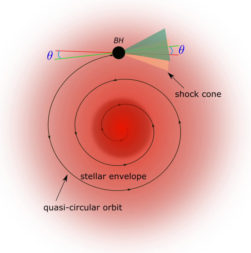
Figure 1.— Schematic diagram – not to scale – of the system being simulated: a black hole moves supersonically in the envelope of a supergiant red star, producing a shock cone in the downstream region of the flow. In doing so, it encounters a density gradient described with the dimensionless parameter $\epsilon_{\rho}$. The modifications of the trajectory can be measured through the deviation of the angle of the shock cone with respect to the upstream flow.

Given the difficulties in modeling the nonlinear processes that take place during the common-envelope evolution, over the years several numerical simulations have been performed, either in one spatial dimension (1D; Taam et al., 1978; Meyer & Meyer-Hofmeister, 1979; Delgado, 1980; Podsiadlowski, 2001; Ivanova et al., 2015; Clayton et al., 2017), in two dimensions (2D; Bodenheimer & Taam, 1984; Armitage & Livio, 2000; Blondin & Pope, 2009; Blondin, 2013), and in three dimensions (3D; Ricker & Taam, 2012; Nandez et al., 2015; MacLeod & Ramirez-Ruiz, 2015a; Ohlmann et al., 2016; Staff et al., 2016; Nandez & Ivanova, 2016; Iaconi et al., 2017; Murguia-Berthier et al., 2017). Overall, this bulk of rather diverse simulations has been able to cover binary systems where the compact object is either a white dwarf, a neutron star or a black hole (see, e.g., MacLeod & Ramirez-Ruiz, 2015a).

A common feature of all of these simulations is that they have been performed within a Newtonian description of gravity. While this may be a reasonable approximation near the central regions of the red supergiant and possibly in the case of a white dwarf, it certainly ceases to be so near the compact object, be it a neutron star or a black hole, and where general relativistic corrections can be considerable. We here present results from the first general relativistic simulations of the common-envelope evolution of a system composed of a red supergiant star interacting with a stellar-mass Schwarzschild black hole; such a system could represent, for instance, the progenitor of the X-ray binary system Cygnus X-3 (Postnov & Yungelson, 2014).

For simplicity, and as a first step in a series of investigations of this process, we here consider the black hole to be a nonrotating (i.e., a Schwarzschild) solution and carry out our simulations in a 2D cut, which is representative of the accretion flow on the equatorial plane. In doing so, we consider the matter in the flow to be a "test matter", hence following the background spacetime geometry of the black hole only; in this way we explicitly neglect the curvature induced by the supergiant stellar core. We also provide analytic expressions for the mass and angular momentum accretion rates and for the angle of the deviation of the shock cone due to drag forces as a function of the density gradient and other reference quantities of the system. Such expressions can represent useful inputs in the phenomenological modeling of the common-envelope evolution.

The plan of the paper is as follows: In Sec. 2 we describe the metric of Schwarzschild spacetime in spherical coordinates written in 3+1 decomposition, the relativistic hydrodynamic equations, and the computational infrastructure employed in their numerical solution via the CAFE code. We also describe the characteristics of the common-envelope scenario we are investigating, the construction of the initial data configurations, and the boundary conditions adopted to guarantee a stationary solution. In Sec. 3 we report our results showing the morphology of the fluid dynamics, the rates of accretion of rest mass and angular momentum, and other related quantities, such as the angle of deviation of the shock cone and the produced bremsstrahlung luminosity. In Sec. 4 we summarize our conclusions and the prospects for future work. Two appendices complement the main text and provide supplemental information. In Appendix A, we calculate the inspiral timescales as derived from our measured accretion rates and explore how the accretion rates are modified by a different prescription for the initial data. In Appendix B, on the other hand, we present convergence tests and a comparison of numerical outcomes from two numerical codes. Hereafter, we will adopt the Einstein convention on sums over repeated indices and use geometrized units where $G=c=1$.

2. Mathematical and numerical setup

2.1. General relativistic hydrodynamics

The simulations carried out involve the solution of the equations of relativistic hydrodynamics in which the matter is considered to behave as a test fluid in the curved spacetime of the astrophysical compact object and thus not to affect it (Rezzolla & Zanotti, 2013). For simplicity, and to build up our physical understanding of the relativistic corrections encountered when studying the evolution of the common-envelope phase in a general relativistic framework, we here consider the background spacetime to be that of a nonrotating black hole of mass $M$, described therefore by the Schwarzschild metric. For the latter and for its convenience in numerical implementation, we use horizon-penetrating Eddington–Finkelstein coordinates in a 3+1 decomposition where the line element of the spacetime is expressed as

$$ds^{2}=-(\alpha^{2}-\beta_{i}\beta^{i})dt^{2}+2\beta_{i}dx^{i}dt+\gamma_{ij}dx^{i}dx^{j}\,,$$ (1)

where $\beta^{i}$ is the shift vector, $\alpha$ is the lapse function, and $\gamma_{ij}$ are the components of the spatial three-metric (Alcubierre, 2008; Rezzolla & Zanotti, 2013). More specifically, the explicit expressions for these functions are given by

$$\alpha = \left(1+\frac{2M}{r}\right)^{-1/2}\,,$$ (2)

$$\beta^{i} = \left(\frac{2M}{r(1+2M/r)},0,0\right)\,,$$ (3)

and

$$\gamma_{ij}=\left(\begin{array}[]{ccc}1+{2M}/{r}&\ \ \ 0&\ \ \ 0\\ 0&\ \ \ r^{2}&\ \ \ 0\\ 0&\ \ \ 0&\ \ \ r^{2}\sin^{2}\theta\end{array}\right)\,.$$ (7)

Given a generic curved spacetime with associated four-metric $g_{\mu\nu}$, e.g., equations (2)–(7), and with associated covariant derivative $\nabla_{\mu}$, the equations of relativistic hydrodynamics can be written as simple conservation laws of the energy-momentum tensor $T^{\mu\nu}$ and of the rest-mass current $J^{\mu}$ (Rezzolla & Zanotti, 2013),

$$\nabla_{\mu}(T^{\mu\nu}) = 0\,,$$ (8)

$$\nabla_{\mu}(J^{\mu})=\nabla_{\mu}(\rho u^{\mu}) = 0\,.$$ (9)

Assuming the fluid to be a perfect one, the corresponding energy-momentum tensor is given by

$$T^{\mu\nu}=\rho hu^{\mu}u^{\nu}+pg^{\mu\nu}\,,$$ (10)

where $\rho$ is the rest-mass density of a fluid element; $u^{\mu}$ is the four-velocity of the fluid; $h=1+\epsilon+p/\rho$ is the specific enthalpy, with $\epsilon$ the specific internal energy; and $p$ the pressure.

The set of relativistic hydrodynamic equations is then closed by an equation of state relating the pressure to other thermodynamics quantities in the fluid. As customary in the calculations of this type, we here assume the equation of state to be that of an ideal fluid, where

$$p=\rho\epsilon(\Gamma-1)\,,$$ (11)

where $\Gamma$ is the adiabatic index, for which we explore the two limits of $\Gamma=5/3$ and $\Gamma=4/3$, corresponding to the properties of a cold degenerate electron fluid and a completely degenerate ultrarelativistic electron fluid, respectively (Rezzolla & Zanotti, 2013).

2.2. Numerical Methods

For the numerical solution of relativistic hydrodynamic equations we employ a conservative formulation, also known as the Valencia formulation (Banyuls et al., 1997), through which a number of important mathematical properties of the set of hyperbolic equations are preserved (Rezzolla & Zanotti, 2013). In our 2D system of spherical azimuthal coordinates representing the orbital (or equatorial) plane of the common-envelope scenario, the relativistic hydrodynamic equations in the Valencia formulation take the form

$$\partial_{t}\bm{U}+\partial_{r}\bm{F}^{r}+\partial_{\phi}\bm{F}^{\phi}=\bm{S}-\frac{1}{2}\partial_{r}\log(\gamma)\bm{F}^{r}\,,$$ (12)

where $\gamma=\det(\gamma_{ij})$ is the determinant of the spatial three-metric and $\bm{U}:=(D,S_{r},S_{\phi},\tau)$ is the vector of the “conserved” variables

$$\bm{U} := (D,S_{r},S_{\phi},\tau)$$ (13)

$$= \left(\rho W,\rho hW^{2}v_{r},\rho hW^{2}v_{\phi},\rho hW^{2}-p-D\right)\,,$$

which depend on the primitive variables with vector $\bm{P}=(\rho,v^{i},p,\epsilon)$. The vectors $\bm{F}^{r}$ and $\bm{F}^{\phi}$ contain instead the “fluxes” along the $r$ and $\phi$ spatial coordinates

$$\bm{F}^{r} = \alpha\left(Dv^{r},S_{r}v^{r}+p\,,S_{\phi}v^{r},(\tau+p)v^{r}\right)\,,$$ (14)

$$\bm{F}^{\phi} = \alpha\left(Dv^{\phi},S_{r}v^{\phi},S_{\phi}v^{\phi}+p,(\tau+p)v^{\phi}\right)\,,$$ (15)

while $\bm{S}$ is the source vector and has explicit components given by

$$\bm{S} = \alpha\left(0,\frac{1}{2}T^{\mu\nu}\partial_{r}g_{\mu\nu},\frac{1}{2}T^{\mu\nu}\partial_{\phi}g_{\mu\nu},T^{\mu t}\partial_{\mu}\alpha-T^{\mu\nu}\Gamma^{t}_{\mu\nu}\alpha\right)\,.$$

Here $\Gamma^{\alpha}_{\mu\mu}$ are the Christoffel symbols, $W:=\alpha u^{0}$ is the Lorentz factor, where $v^{i}$ and $v_{i}=\gamma_{ij}v^{j}$ are the components of the spatial three-velocity of the fluid measured by a (normal) Eulerian observer. These three-velocities are related to the spatial components of the four-velocity by $v^{i}=u^{i}/W+\beta^{i}/\alpha$.

The relativistic hydrodynamic equations are solved numerically using high-resolution shock-capturing methods (HRSC; Rezzolla & Zanotti, 2013) and, in particular, the Harten, Lax, van Leer, and Einfeldt (HLLE) approximate Riemann solver (Harten et al., 1983; Einfeldt et al., 1991) combined with the "minmod” second-order total variation diminishing (TVD) reconstruction approach at cell interfaces (see Keppens et al., 2012; Porth et al., 2017, for more details). The time evolution of the set of partial differential equations is realized via a method-of-lines approach and a third-order Runge-Kutta scheme, which guarantees the TVD property (Shu & Osher, 1988).

As mentioned above, the numerical code employed for the numerical solution is the CAFE code, which has been developed to solve the equations of relativistic hydrodynamics in 2D slab symmetry (Cruz-Osorio et al., 2012; Lora-Clavijo et al., 2015b; Cruz-Osorio & Lora-Clavijo, 2016), 2D axial symmetry (Lora-Clavijo & Guzmán, 2013), and magnetohydrodynamics (MHD) in 3D (Lora-Clavijo et al., 2015a). The numerical grid employs radial and azimuthal coordinates and is uniformly spaced with $N_{r}\times N_{\phi}=2000\times 256$ cells. The radial grid, in particular, extends from $r_{\rm exc}$ to $r_{\rm max}$, where $r_{\rm exc}$ is the excision radius that is located inside the event horizon, i.e., at $r_{\rm exc}=1.5\,M\,(\sim 8.9\,{\rm km})$ and $r_{\rm max}=10\,r_{\rm acc}\,\sim(1190\,{\rm km})$ is expressed in terms of the accretion radius, $r_{\rm acc}$, whose definition is discussed below; the angular coordinate, $\phi$, on the other hand, spans the full internal $\phi\in[0,2\pi]$. The effective resolution $(\Delta r,\Delta\phi)=(0.1\,M,0.0386\,{\rm rad})$ in geometrized units, or, equivalently, $\Delta r\sim 0.6\,{\rm km}$. Finally, the timestep size is constant and satisfies the Courant-Friedrich-Lewy (CFL) stability condition, with $\Delta t=\tfrac{1}{4}\,\min(\Delta r,\Delta\phi)$.

2.3. Common-envelope setup

In our modeling, we assume that the common-envelope phase takes place in a binary system composed of a stellar-mass black hole with mass $M$ and a more massive red supergiant with mass $M_{\rm star}$ and radius $R_{\rm star}$. This scenario could occur either after the collapse of a neutron star to a black hole in a binary system initially containing a red supergiant and a neutron star or in a binary system with a red supergiant and a massive star that collapse directly to a black hole (Postnov & Yungelson, 2014; MacLeod & Ramirez-Ruiz, 2015a). Assuming furthermore that the binary is in a quasi-circular orbit with radius $R$, the black hole will have a Newtonian linear velocity that can be easily estimated from the Keplerian motion to be $v_{{}_{\rm CE}}=(m(R)+M)/R$, where $m(R)$ is the mass enclosed in a sphere with radius $R$, the latter being necessarily $R<R_{\rm star}$ within the common-envelope phase. Because it is numerically convenient to place the black hole at the center of our coordinate system and to consider therefore the relative motion of the stellar envelope, we can reverse the reference systems and thus take the asymptotic velocity of the fluid $v_{\infty}$ as $v_{{}_{\rm CE}}=v_{\infty}$. We note that, strictly speaking, the Keplerian velocity at these separations is $\mathcal{O}(10^{2}-10^{3})\,{\rm km/s}$ giving velocities $\mathcal{O}(10^{-3}-10^{-4})\,{\rm c}$, in geometrical units and thus too small to be used in numerical simulations. However, as long as the proper Mach number is chosen for the simulations (i.e., $\mathcal{M}=1-5$ for typical common-envelope scenarios; MacLeod et al. 2017), it is possible to perform simulations with effectively larger velocities (i.e., $\mathcal{O}(10^{4})\,{\rm km/s}$ in our case) and then rescale all the results to smaller initial velocities through scaling relations (see Equations (31) and (32) and discussion in Sec. 3.2 and Appendix A.2). A very similar approach has already been employed by MacLeod & Ramirez-Ruiz (2015a) and MacLeod et al. (2017), who have used $v_{\infty}=1$ in a fully Newtonian context.

Also for the rest-mass density distribution, we make the rather simplified but reasonable assumption that it is given by a constant-density core of density $\bar{\rho}$ and that then falls exponentially up to the surface. Assuming a coordinate system with origin in the center on the star, we thus express the rest-mass density as

$$\rho(r)=\begin{cases}\bar{\rho}={\rm const.}\quad&{\rm for}\quad 0<r<\bar{r}\\ \rho_{0}\exp{\left[-\epsilon_{\rho}(r-r_{0})/r_{\rm acc}\right]}\,,\quad&{\rm for}\quad\bar{r}\leq r\leq R_{\rm star}\end{cases}$$ (17)

where $r_{0}>\bar{r}$ is the radial position of the black hole within the common envelope (see below) and $\rho_{0}$ is the rest-mass density at that position (i.e., $\rho_{0}:=\rho(r=r_{0})$); clearly, from expression (17) it follows that $\bar{\rho}:=\rho(r=\bar{r})>\rho_{0}$. Note also that we have introduced the "accretion radius”, $r_{\rm acc}$, which represents the length scale over which the gravitational effects of the compact object dominate over the dynamics of the fluid, and which naturally appears when considering the problem of accretion onto a compact object moving in a medium, i.e., a Bondi–Hoyle–Lyttleton accretion (Hoyle & Lyttleton, 1939; Bondi & Hoyle, 1944; Rezzolla & Zanotti, 2013). Its definition is therefore

$$r_{\rm acc}:=\frac{M}{c^{2}_{s,\infty}+v^{2}_{\infty}}=\frac{M}{c^{2}_{s,\infty}(1+{\cal M}^{2}_{\infty})}\,,$$ (18)

and thus in terms of the asymptotic value of Newtonian Mach number ${\cal M}_{\infty}:=v_{\infty}/c_{s,\infty}$, where $c_{s,\infty}$ is the asymptotic sound speed. As will become clearer when we introduce the reference mass accretion rate (see Equation (24)), the accretion radius (18) plays a fundamental role in establishing what is the amount of matter that is accreted onto the black hole. More importantly, the accretion radius (and hence the mass accretion rate) depends not only on the asymptotic velocity $v_{\infty}$, but also on the asymptotic sound speed $c_{s,\infty}$.

Arguably, among the most important quantity in the description of the common-envelope evolution is the strength of the density gradient that the compact object experiences as it moves in the stellar envelope. A convenient way to express this contrast is to normalize the rest-mass density scale height

$$\mathcal{L}_{\rho}:=-\frac{\rho}{d\rho/dr}\,,$$ (19)

with the other characteristic length scale of the problem, namely, the accretion radius, to obtain the “dimensionless accretion radius”

$$\epsilon_{\rho}:=-r_{\rm acc}\frac{d\rho/dr}{\rho}=\frac{r_{\rm acc}}{\mathcal{L}_{\rho}}\,.$$ (20)

In practice, $\epsilon_{\rho}$ is here treated as a free parameter, and in the simulations we have explored various values, which are summarized in Tab. 1.

2.4. Initial and boundary conditions

For the initial stellar model we follow the prescription presented by MacLeod & Ramirez-Ruiz (2015a), thus assuming a binary system composed of a red supergiant star with mass $M_{\rm star}=16\,M_{\odot}$ and a stellar-mass black hole with mass $M=4\,M_{\odot}$, so that the corresponding mass ratio in the binary is $q:=M/M_{\rm star}=0.25$. The black hole is placed at $r_{0}=R_{\rm star}/2\simeq 400\,R_{\odot}\simeq 2.78\times 10^{8}\,{\rm km}$ and the rest-mass density there is assumed to be $\rho(r_{0})=:\rho_{0}=\rho_{\infty}\simeq 9.51\times 10^{-9}\,{\rm g/cm}^{3}$. With such a value and an intermediate value for the density gradient $\epsilon_{\rho}=0.5$, the integration of the rest-mass density (17) yields a supergiant star with 16 $M_{\odot}$.

For such a system, the merger timescale is given by (Faber & Rasio, 2012)

$$\tau_{\rm merg}=2.2\times 10^{8}\frac{1}{4q(1+q)}\left(\frac{a}{R_{\odot}}\right)^{4}\left(\frac{M_{\rm star}}{1.4\,M_{\odot}}\right)^{-3}\ {\rm yr}\,,$$ (21)

and because our simulations are carried out over a timescale of $\tau_{\rm sim}\simeq 20000\,M_{\odot}\sim 0.1\,{\rm sec}$, it is perfectly reasonable to assume that the density profile does not to change over the time of the simulations.

In the reference frame where the black hole is at rest, the common-envelope material is seen moving moving at a constant velocity that is uniform within the computational domain and set assuming that the sound speed of the fluid is $c_{s,\infty}=0.1$ and that the fluid is supersonic with Mach number ${\cal M}_{\infty}=2$ (as a result, the asymptotic fluid velocity is $v_{\infty}=0.2$).

After mapping the spherical polar coordinate system $(r,\phi)$ to a Cartesian $(x,y)$ system where the stellar center is at the position $(x_{0},y_{0})$ (see Cruz-Osorio et al., 2012, for more details on the mapping), the common envelope is taken to be moving in the positive $x$-direction, i.e., $v^{x}=v_{\infty}$, and the matter is taken to have a rest-mass gradient only in the $y$-direction (see Equation (17)). As a result, the initial rest-mass density profile is set to be $\rho_{\rm in}:=\rho(y)=\rho_{0}\exp{\left[-\epsilon_{\rho}y/r_{\rm acc}\right]}$, where $y\in[-\bar{r},\bar{r}]$, and we set the edge of our numerical grid to coincide with the edge of the constant-density stellar core, i.e., $r_{\rm max}=\bar{r}=10\,r_{\rm acc}$. The resulting accretion radius after substituting the asymptotic sound speed and the asymptotic velocity in Eq. (18) is $r_{\rm acc}=20\,M\sim 119\,{\rm km}$.

Once a choice is made for the initial rest-mass density distribution and the equation of state has been fixed to be that of an ideal fluid, the initial pressure is determined by the definition of the sound speed as

$$p_{\rm in}=c^{2}_{s,\infty}\frac{\Gamma-1}{\Gamma(\Gamma-1)-c^{2}_{s,\infty}\Gamma}\,\rho_{\rm in}\,,$$ (22)

where we have made use of the fact that initially the fluid is isentropic and hence it can also be described by a polytropic equation of state (Cruz-Osorio et al., 2012).

The initial distributions of the rest-mass density of the common envelope are plotted in Fig. 2, from right to left $\epsilon_{\rho}=0.0,0.5$ and $1.0$, which can be interpreted as different stages of the common-envelope evolution. More specifically, as the distance between the black hole and the center of the supergiant decreases, the density gradients increase, thus going from $\epsilon_{\rho}\sim 0.0$ to $\epsilon_{\rho}\sim 1.0$, where the differences in the density at $y$-axis are $\Delta\rho=0$ to $\Delta\rho=10^{8}$, respectively, while the streamlines (depicted with white lines) show a uniform velocity in the $x$-direction.

Table 1Summary of the models considered, all of which refer to a Schwarzschild black hole, have a fixed sound speed of $c_{s,\infty}=0.1$, and an asymptotic Mach number ${\cal M}_{\infty}=2$, corresponding to an asymptotic velocity $v_{\infty}=0.2$; this choice fixes the accretion radius $r_{\rm acc}$ (in mass units and in kilometers) to the value reported in the fourth column. Hence, the parameters varied are the values of the adiabatic index $\Gamma$ and of the rest-mass density relative scale height $\epsilon_{\rho}$. Finally, shown in the last column is the resolution in the radial direction $\Delta r$.

Model	$\epsilon_{\rho}$	${\Gamma}$	$r_{\rm acc}[M\,({\rm km})]$	$\Delta r[M\,({\rm km})]$
RCE.0.0.5o3	$0.0$	$5/3$	$20\,(119)$	$0.1\,(0.6)$
RCE.0.1.5o3	$0.1$	$5/3$	$20\,(119)$	$0.1\,(0.6)$
RCE.0.3.5o3	$0.3$	$5/3$	$20\,(119)$	$0.1\,(0.6)$
RCE.0.5.5o3	$0.5$	$5/3$	$20\,(119)$	$0.1\,(0.6)$
RCE.0.7.5o3	$0.7$	$5/3$	$20\,(119)$	$0.1\,(0.6)$
RCE.1.0.5o3	$1.0$	$5/3$	$20\,(119)$	$0.1\,(0.6)$
RCE.0.0.4o3	$0.0$	$4/3$	$20\,(119)$	$0.1\,(0.6)$
RCE.0.1.4o3	$0.1$	$4/3$	$20\,(119)$	$0.1\,(0.6)$
RCE.0.3.4o3	$0.3$	$4/3$	$20\,(119)$	$0.1\,(0.6)$
RCE.0.5.4o3	$0.5$	$4/3$	$20\,(119)$	$0.1\,(0.6)$
RCE.0.7.4o3	$0.7$	$4/3$	$20\,(119)$	$0.1\,(0.6)$
RCE.1.0.4o3	$1.0$	$4/3$	$20\,(119)$	$0.1\,(0.6)$

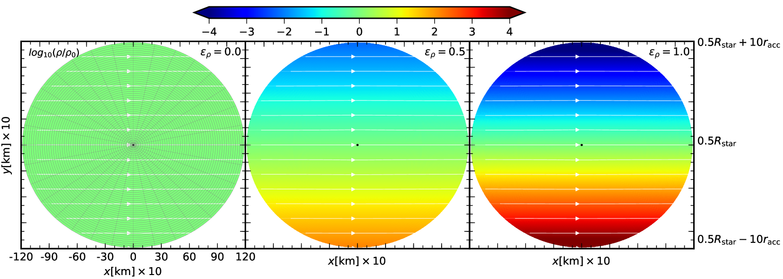
Figure 2.— Initial distributions of the rest-mass density and the velocity field streamlines in the common envelope projected on the $x-y$ plane for models RCE.0.0.5o3, RCE.0.5.5o3 and RCE.1.0.5o3 with adiabatic index $\Gamma=5/3$ and for the dimensionless density gradients $\epsilon_{\rho}=0.0,0.5$, and $1.0$, respectively. In the left panel we overplot some of the grid lines ($1/40$ and $1/8$ in the radial and azimuthal direction, respectively) used in the numerical simulations. All axes have units of $\rm km$, with the exception of the vertical right vertical axis, which is expressed in terms of radius of the star and of the accretion radius $r_{\rm acc}$. Note that the black hole is located at the center of the numerical domain (shown with a black circle), which covers only a small fraction of the star radius $20\,r_{\rm acc}\sim 4.3\times 10^{-6}R_{\rm star}$.

Finally, when discussing the boundary conditions, we recall that the inner boundary $r_{\rm exc}$ is always situated inside the event horizon, where we apply an inward extrapolation of the conservative variables in the state vector $\bm{U}$. On the other hand, on the external boundary at $r_{\rm max}$ we impose a steady inflow of matter having the same properties in terms of density, pressure, and velocity given by the initial conditions, assuming an inflow in the upstream part of the computational domain, i.e., for $\pi/2<\phi<3\pi/2$, and an outflow in the downstream part, i.e., for $-\pi/2<\phi<\pi/2$. Finally, we impose simple periodic boundary conditions in the $\phi$-direction.

3. Results

3.1. Morphology of the accreting plasma

The morphology of the evolved common envelope as sketched in the cartoon in Fig. 1 – black hole moving perpendicular to the direction of the gradient – is shown in Fig. 3, where we report, for the $\Gamma=4/3$ case, the different panels: the rest-mass density (left panel), the temperature (left panel), and the Mach number $\mathcal{M}:=Wv/W_{s}c_{s}$, where $W_{s}$ is the Lorentz factor of the sound speed (right panel). The snapshots refer to $t\sim 5000M\,\sim 0.1\,{\rm s}$, which is obviously much shorter than the typical evolution timescale of a common-envelope scenario. On the other hand, this time corresponds to $\sim 50$ crossing times, when the gas has reached a steady state and serves therefore as a useful reference for the stationary dynamics of the system. More specifically, the different rows of Fig. 3 refer to different values of the dimensionless density gradient, i.e., $\epsilon_{\rho}=0,\ 0.5$ and $1.0$ from top to bottom, where the case with $\epsilon_{\rho}=0$ corresponds to a constant rest-mass density profile. A magnified view of the same panels is offered in Fig. 4 and helps us appreciate the dynamics of the flow in the vicinity of the black hole.

The temperature in the central column of Figs. 3 to 5 was computed using the definition from (Zanotti et al., 2010),

$$T = 1.088\times 10^{13}\left(\frac{p}{\rho}\right)K\,,$$ (23)

where the numerical factor comes from the transformation from geometric units to Kelvin.

We start by considering the behaviour of the accretion of a fluid with $\Gamma=4/3$ as reported in Figs. 3 and 4. The dynamics observed in the case of the motion across a constant-density cloud reproduces well the behavior observed in simulations of Bondi–Hoyle accretion, where the shock cone in the wake of the black hole is stable and symmetric with respect to the to direction of motion, i.e., the $x$-axis in this case (see, e.g., Font et al., 1999; Dönmez et al., 2011; Cruz-Osorio et al., 2012; Lora-Clavijo et al., 2015b) . This is highlighted in Figs. 3 and 4 by the streamlines of the flow (white lines) and by the moderate compression in the matter density around the black hole, which shows an increase of less than two orders of magnitude in the rest-mass density.

On the other hand, the dynamics produced in models RCE.0.5* and RCE.1.0* shows that, once formed, the shock cone is stationary but tends to be directed along the direction of the gradient in the rest-mass density, and hence pointing away from the region of high density in the cloud, namely, the center of the red supergiant. Note, however, that as the dimensionless accretion radius is increased, the density profile along the direction of motion of the black hole develops an asymmetry, with a low-density region ahead of the black hole and a corresponding high-density region behind. As a result, the shock cone – which is aligned along the direction of motion (i.e., the horizontal direction in our setup) for a uniform medium – is now dragged by the density gradient and tends to align with it for $\epsilon_{\rho}=0.5$.

This is shown in the left panels of Figs. 3 and 4, both of which refer to the case with $\Gamma=4/3$ and show different scales of the computational domain. In these figures, from top to bottom, the gradual increase in the density gradient – which can be taken to mimic the motion of the black hole as it gets closer to the core of the red supergiant – leads to an increasingly large angle with respect to the direction of motion (see the diagram in Fig. 1), which can be larger than $\pi/2$ for the case of the largest value of the initial gradient $\epsilon_{\rho}=1.0$ (bottom row). Interestingly, in the latter case, most of the motion downstream of the black hole is actually away from the core of the supergiant.

The motion of the matter is best followed through the streamlines of fluid elements and shown in the left column of Figs. 3 and 4. When contrasting the top and bottom rows, it is possible to appreciate that while the fluid elements always move in the positive $x$-direction in the case of a medium that is uniform or with a small density gradient (top and middle row), they can also move in the negative $x$-direction in the case of a large density gradient (bottom row). However, in contrast with what was reported in the Newtonian simulations of MacLeod et al. (2017), no significant vorticity is found in these regimes; while a vortical motion may well be produced at even larger density gradients, the stronger general relativistic gravitational fields prevent their formation here.

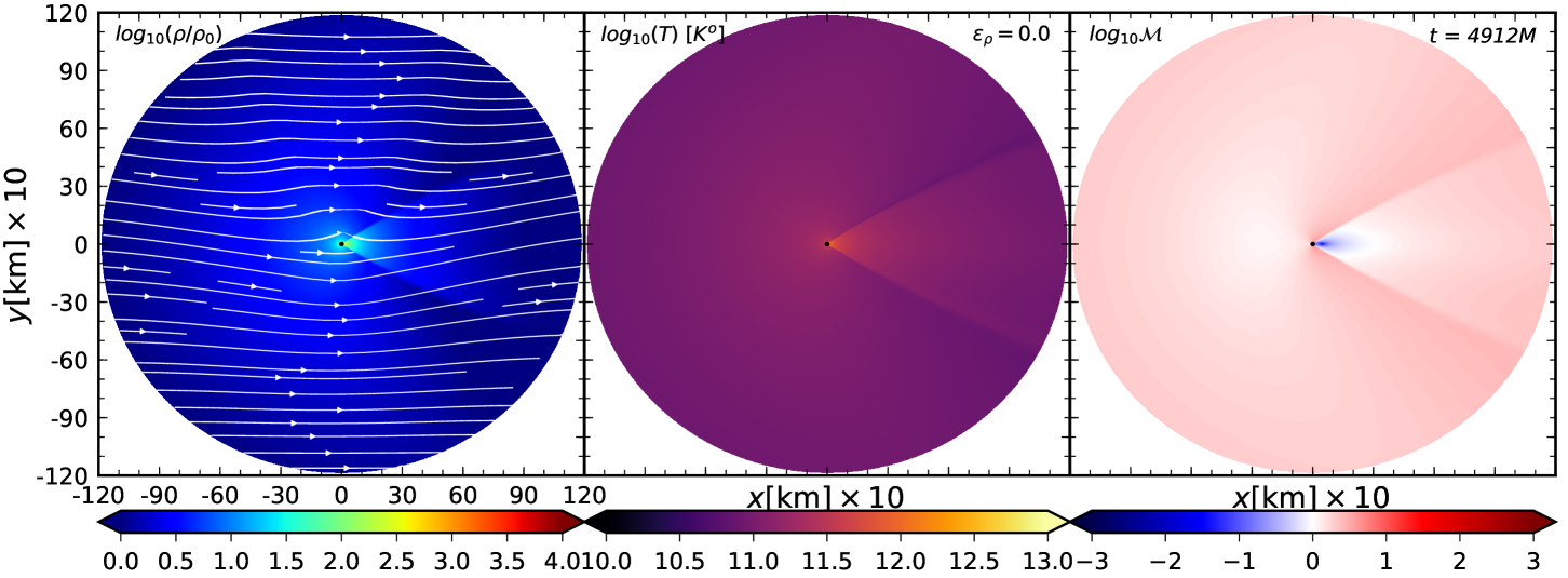
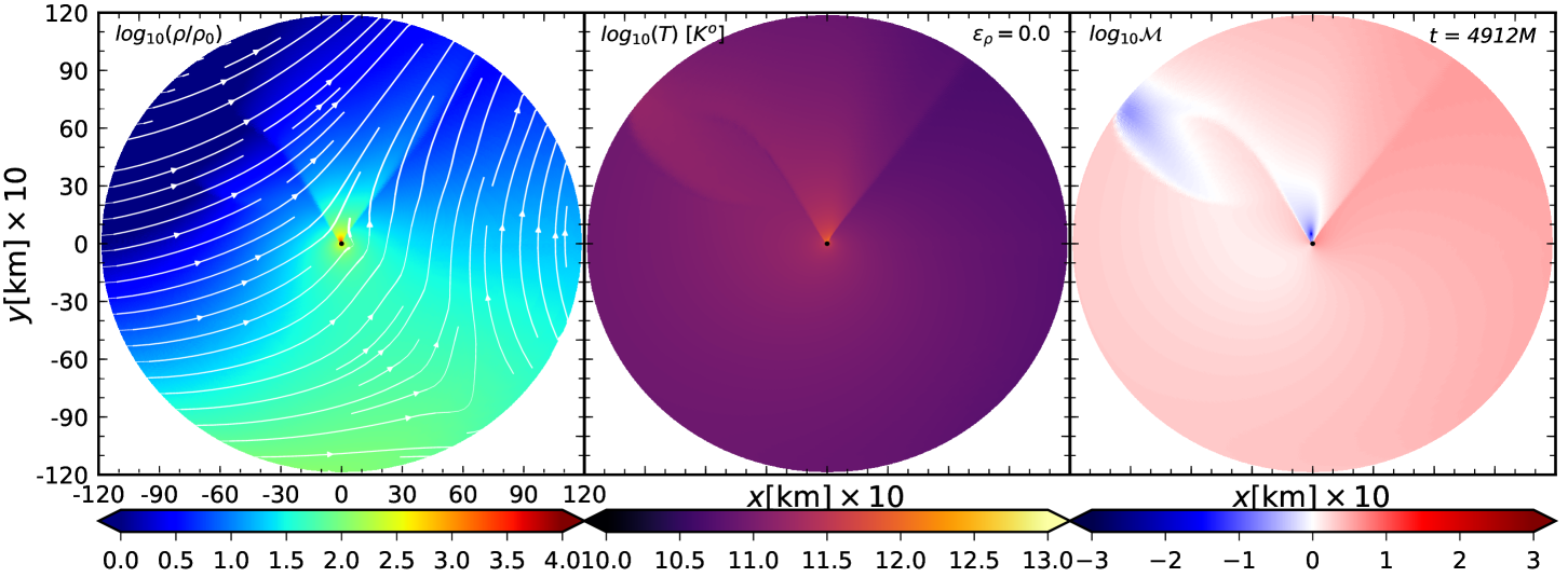
Figure 3.— Snapshots of the rest-mass density, temperature, and Mach number at the end of our numerical simulations $t\sim 5000\,M\sim 0.1\,{\rm s}$ for models RCE.0.0.4o3, RCE.0.5.4o3 and RCE.1.0.4o3. From top to bottom, we show the morphology of the accreting matter envelope for dimensionless density gradients of $\epsilon_{\rho=}0,0.5$, and $1.0$. In all panels, the adiabatic index is set to $\Gamma=4/3$.

The development of the shock cone heats up the fluid, leading to a temperature increase that is about one order of magnitude larger than in the rest of the envelope, with a fluid that is overall two orders of magnitude hotter than in the initial state (see central columns in Figs. 3 and 4). As is well known in the phenomenology of Bondi–Hoyle–Lyttleton accretion across a uniform medium, a stagnation point develops in the shock cone, with some of the material into the shock cone accreting subsonically onto a black hole (i.e., ${\cal M}\sim 10^{-1}$). These regions are shown in blue in the right columns of Figs. 3 and 4, which refer to the Mach number. Interestingly, the dragging of the shock cone also leads to the formation of a stagnating subsonic flow in the presence of a density gradient, which becomes increasingly severe as the gradient is increased (middle and bottom rows). In this case, large variations in the Mach number are produced, with variations of almost two orders of magnitude.

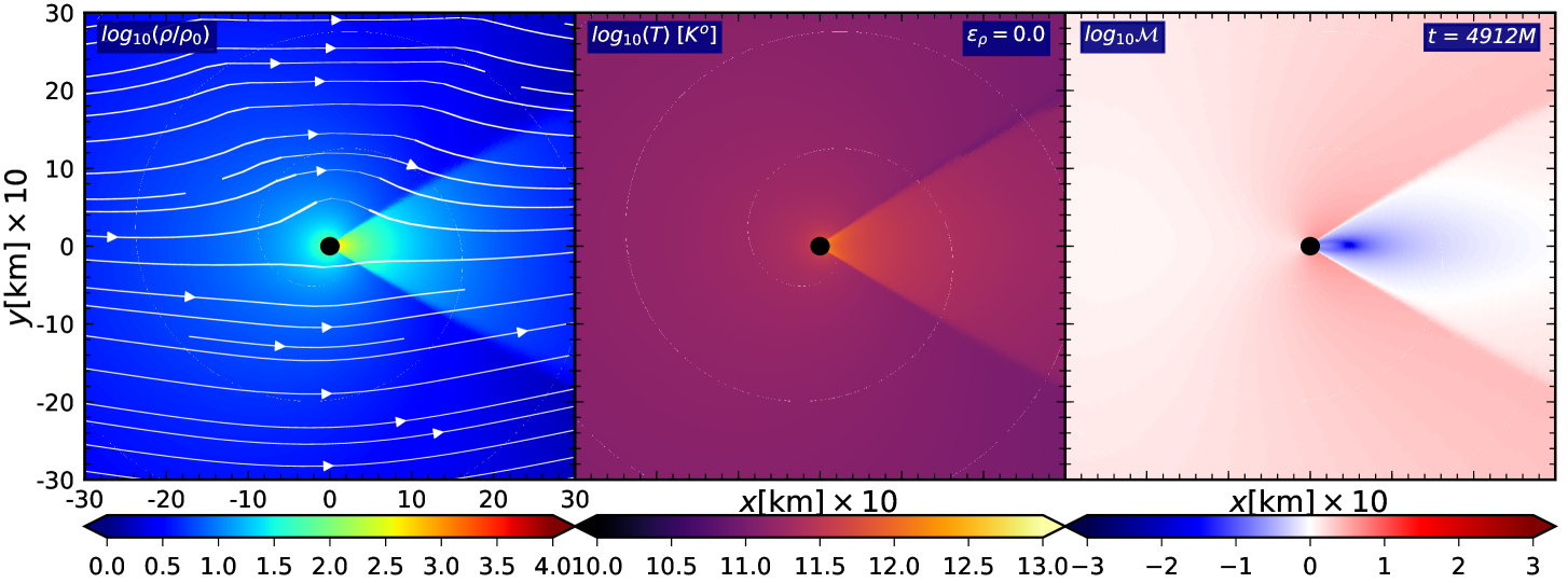
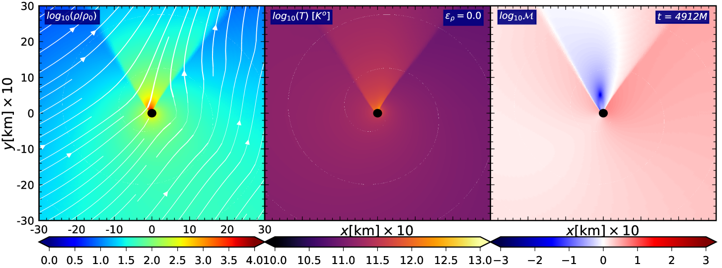
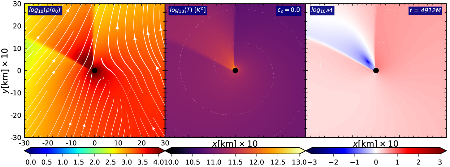
Figure 4.— Close-up view of the various panels of Fig. 3 to highlight the dynamics near the accreting black hole.

When changing the adiabatic index, that is, when considering the same setups but for an ideal-fluid equation of state with $\Gamma=5/3$, and hence considering a different compressibility of the gas in the common envelope, no major qualitative differences appear in the overall properties of the flow, although quantitative differences do emerge and will be measured in the following sections. Besides slightly larger temperatures (of about a factor of two), the most significant difference that emerges in simulations with $\Gamma=5/3$ is the clear appearance of a bow shock in the upstream region of the flow and that follows the rotations of the shock cone as the density gradient is increased (see Fig. 5). Before concluding this section on the overall dynamics of the flow, we should note that in our simulations the bow shock appears only for $\Gamma=5/3$, unlike in the Newtonian case (MacLeod & Ramirez-Ruiz, 2015a; MacLeod et al., 2017), where it is present also for $\Gamma=4/3$.

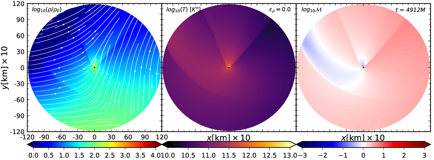
Figure 5.— Same as in Fig. 3, but for models RCE0.0.5o3, RCE.0.5.5o3, and RCE.1.0.5o3. In all panels, the adiabatic index is set to $\Gamma=5/3$.

3.2. Mass accretion and drag rates

Besides a general understanding of the dynamics of the plasma as it interacts with the black hole – which has an interest of its own – our simulations are meant to also measure the typical rates of accretion of mass and momentum, since the latter have important implications on the quantitative description of the common-envelope evolution. In the case of spherical accretion onto a black hole and an ideal-fluid equation of state, analytic expressions can be obtained for the accretion rates of mass and momentum (Petrich et al., 1989; Rezzolla & Zanotti, 2013)

$$\dot{M}_{\rm ref} = 4\pi\lambda\rho_{\infty}M^{1/2}r^{3/2}_{\rm acc}\,,$$ (24)

$$\dot{P}_{\rm ref} = \dot{M}_{\rm ref}\frac{v_{\infty}}{\sqrt{1-v^{2}_{\infty}}}\,,$$ (25)

where

$$\lambda := \left(\frac{1}{2}\right)^{(\Gamma+1)/(2(\Gamma-1))}\left(\frac{5-3\Gamma}{4}\right)^{-(5-3\Gamma)/(2(\Gamma-1))}$$ (28)

$$\simeq \left\{\begin{array}[]{lr}0.71&\qquad(\Gamma=4/3)\\ 0.25&\qquad(\Gamma=5/3)\end{array}\right.\,.$$

Equations (24) and (25) will be used hereafter as a reference values to express the numerically computed mass accretion and drag rates (also referred to as “momentum accretion rates”), which we compute as (Petrich et al., 1989)

$$\dot{M} = \int_{0}^{2\pi}\alpha\sqrt{\gamma}D(v^{r}-\beta^{r}/\alpha)d\phi\,,$$ (29)

$$\dot{P}^{i} = -\int_{\partial V}\alpha\sqrt{\gamma}T^{ij}d\Sigma_{j}+\int_{V}\alpha\sqrt{\gamma}S^{i}dV\,.$$ (30)

where $i=r,\phi$, and the inward fluxes are measured at the event horizon.

In Fig. 6 we report the mass accretion rates as a function of time for the various models considered. Note that all models reach a stationary accretion state after about 20 crossing times, and we use such asymptotic values to construct the data shown in Fig. 7, which provides a summary of the mass accretion for all of the cases considered in terms of the dimensionless density gradient $\epsilon_{\rho}$ and equation of state; also reported for comparison are the values presented by MacLeod & Ramirez-Ruiz (2015a) for their simulations in Newtonian gravity. Note that for configurations with a zero density gradient ($\epsilon_{\rho}=0$), we reproduce the expected super-Eddington accretion rate ($\dot{M}\sim 10^{-8}$) for Bondi–Hoyle–Lyttleton accretion obtained also in previous simulations (Zanotti et al., 2010, 2011; Lora-Clavijo et al., 2015b); furthermore, these values have been cross-checked also with a different general relativistic MHD code (see discussion in Appendix B). Figure 8 reports a very similar behavior also for the rates of accretion of radial momentum (left panel) and of angular momentum (right panel).

Figure 7 also shows that, for non-negligible density gradients, i.e., $\epsilon_{\rho}\gtrsim 0.3$, both the mass accretion rate and the drag rate grow exponentially with the density gradient and can therefore be well approximated with functions of the type

$$\log\left(\frac{\dot{M}}{\dot{M}_{\rm ref}}\right) = \mu_{1}+{\mu_{2}}/({1+\mu_{3}\epsilon_{\rho}+\mu_{4}\epsilon^{2}_{\rho}})\,,$$ (31)

$$\log\left(\frac{\dot{P}^{\phi}}{\dot{P}_{\rm ref}}\right) = \wp_{1}+\wp_{2}\epsilon_{\rho}+\wp_{3}\epsilon^{2}_{\rho}\,,$$ (32)

where the values of the fitting coefficients $\mu_{i}$ and $\wp_{i}$ are reported in the Table 2 for the two adiabatic indices $\Gamma=5/3$ and $\Gamma=4/3$. Using expressions (31) and (32) it is possible to obtain mass accretion rates also when considering different initial conditions as long as they are not very different from those considered here (see also the discussion in Appendix A.2). For example, given $\left({\dot{M}}/{\dot{M}_{\rm ref}}\right)_{\rm old}$ as expressed by Equation (31), if one wishes to calculate a new mass accretion rate $(\dot{M})_{\rm new}$ using a different initial velocity or rest-mass density, it is sufficient to take into account the changes introduced by the new accretion radius in the reference mass accretion rate $(\dot{M}_{\rm ref})_{\rm new}$ so that $(\dot{M})_{\rm new}=(\dot{M}_{\rm ref})_{\rm new}\left({\dot{M}}/{\dot{M}_{\rm ref}}\right)_{\rm old}$.

Figure 6.— Evolution of the mass accretion rates for the adiabatic indices $\Gamma=4/3$ (solid lines) and $\Gamma=5/3$ (dotted lines). In all models, the accretion process reaches a stationary state after about 10 crossing times. Note that the low-$\epsilon_{\rho}$ curves are rescaled to appear on the same plot.

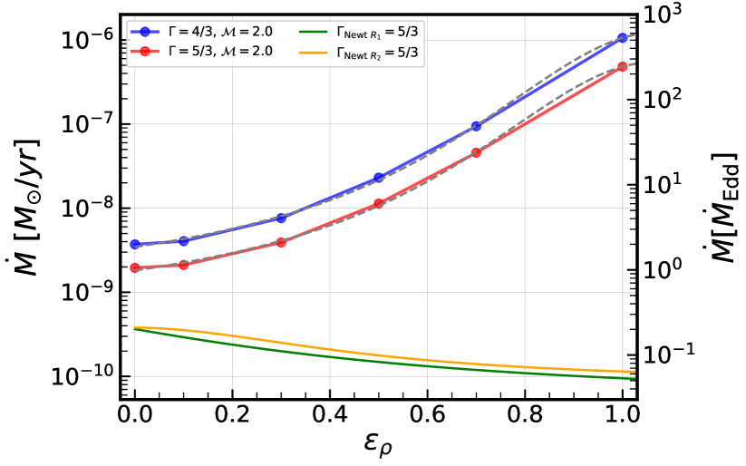
Figure 7.— Mass accretion rates – expressed either in solar masses per year or in Eddington rates – computed at the event horizon and shown as a function of the dimensionless density gradient $\epsilon_{\rho}$. Shown with blue and red lines are the results for a fluid with $\Gamma=4/3$ and $\Gamma=5/3$, respectively. Also shown are the corresponding rates as reported in Newtonian simulations and when computed at two different radii, i.e., $R_{1}=0.01r_{\rm acc}$ and $R_{1}=0.05r_{\rm acc}$ (MacLeod & Ramirez-Ruiz, 2015a). Note that while the general relativistic rates grow almost exponentially with $\epsilon_{\rho}$, the Newtonian ones decrease.

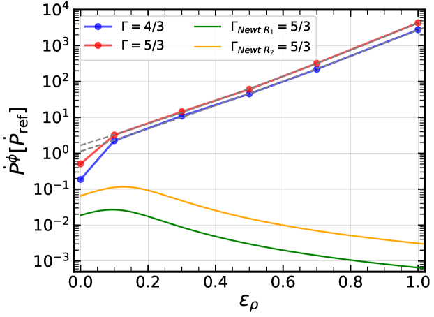
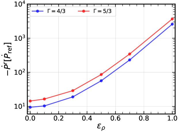
Figure 8.— Same as in Fig. 7 but for the accretion of angular momentum (left) and of radial momentum (right). Also in this case, note that while the general relativistic rates grow almost exponentially with $\epsilon_{\rho}$, the Newtonian ones decrease.

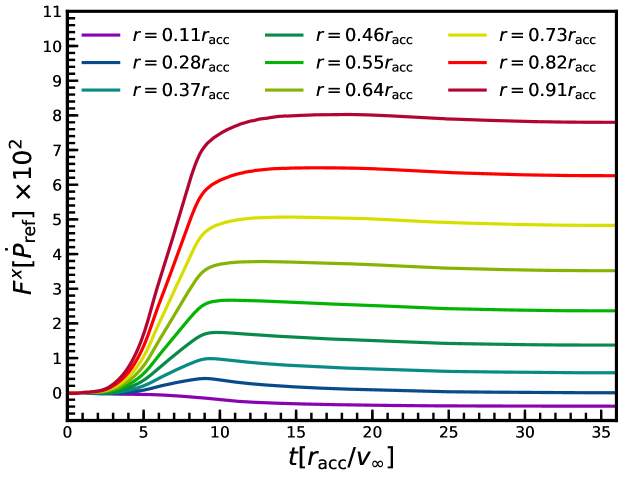
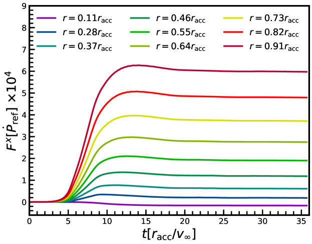
Figure 9.— Total drag force along the $x$-direction (see Equation (33)) produced by the combination of the accretion of linear momentum and that of the dynamical friction. The different lines refer to the different spherical surfaces where the fluxes are computed (expressed in terms of the accretion radius), while the top and bottom panels refer to dimensionless density gradients of $\epsilon_{\rho}=0.5$ and $\epsilon_{\rho}=1.0$, respectively.

When comparing the results of the mass accretion rates in the top panel of Fig. 7 and 8 with the corresponding nonrelativistic values in Newtonian gravity (MacLeod & Ramirez-Ruiz, 2015a), the most striking difference is in the dependence from the density gradient. While, in fact, the two accretion rates are comparable for small gradients, the relativistic ones grow with $\epsilon_{\rho}$, the opposite is true in the non-relativistic case. It is presently difficult to ascertain the origin of this difference, but it may ultimately be associated with the stronger gravitational fields that the fluid experiences in our simulations. Indeed, a mass accretion rate that increases with the density contrast is rather natural to expect since the local rest-mass density near the black hole will be intrinsically large. On the other hand, this behavior is not found in a Newtonian regime because of the appearance there of disk-like structures with nonzero angular momentum that suppress the infall of the matter toward the black hole. As mentioned above, no such vortical motions emerge in our simulations.

Very similar considerations apply also when comparing the relativistic and Newtonian drag rates (bottom panel of Fig. 7). Also in this case, in fact, the relativistic drag rates – which are ultimately responsible for the loss of orbital angular momentum in the binary system and thus to the decrease in the orbital period (Taam & Ricker, 2010) – increase with the density gradient (as one would naturally expect), while they decrease in the Newtonian case. Once again, this different behavior may be due to the different role played by the gravitational forces. On the other hand, it may also be due to the different boundary conditions, which in our case are imposed inside the event horizon by using the ingoing Eddington–Finkelstein coordinates and are those of a purely infalling gas. A more involved description is instead adopted in the Newtonian calculations of MacLeod & Ramirez-Ruiz (2015a), where spherical absorbing boundary conditions are applied to a “sink” surrounding the central point mass, whose gravitational potential of the point mass is smoothed within this sink.

Table 2Fitting coefficients for the mass accretion rate and the drag rate given by Eqs. (31) and (32), respectively.

$\Gamma$	$\mu_{1}$	$\mu_{2}$	$\mu_{3}$	$\mu_{4}$	$\wp_{1}$	$\wp_{2}$	$\wp_{3}$
$4/3$	$-0.29$	$1.39$	$-1.52$	$0.70$	$0.13$	$7.06$	$0.72$
$5/3$	$0.18$	$1.24$	$-1.54$	$0.72$	$0.51$	$6.69$	$1.16$

3.3. Drag forces, drag angle, and emitted radiation

Drag forces experimented by the black hole as it moves in the envelope of the red supergiant star are responsible for its deceleration. Estimating these forces in a fully general relativistic context is of course possible, but it is also less transparent than in a simpler Newtonian description. In view of this, and in order to make the comparison with previous Newtonian estimates simpler, we will hereafter adopt a hybrid framework in which we use the simpler Newtonian expressions for the drag forces but evaluate the mass and momentum fluxes needed for these expressions within in a full general relativistic prescription. Hence, we write the total drag force in the $i$th direction as

$$F^{i}=F^{i}_{\rm drag}+F^{i}_{\rm dyn}\,,$$ (33)

where the first contribution is due to the accretion of the linear momentum and we compute it as

$$F^{i}_{\rm drag}=\frac{1}{\Sigma}\int\alpha\sqrt{\gamma}\big{(}\dot{\bm{P}}\cdot\bm{x}\big{)}^{i}d\Sigma\,,$$ (34)

where $\Sigma$ is a spherical surface at a given distance from the black hole, $\bm{e}_{x}$ is the unit vector in the direction of motion of the black hole (the negative $x$-direction in our setup), and $\dot{P}^{i}$ is computed using Eq. (30). The second contribution is instead due to dynamical friction arising from the interaction of the black hole with the matter of the common envelope (Ostriker, 1999; Barausse, 2007; Barausse & Rezzolla, 2008).

Starting from the Newtonian approximation to the infinitesimal dynamical friction force $dF_{\rm dyn}$ produced by fluid element of density $\rho$ in a volume $dV$, i.e., $d\bm{F}_{\rm dyn}=M\rho\,dV\bm{r}/r^{2}$ (see Equation (26) of MacLeod et al. (2017)), we express the relativistic dynamical friction as

$$F^{i}_{\rm dyn}=M\int\alpha\sqrt{\gamma}D\left(\frac{\bm{e}_{r}\cdot\bm{e}_{x}}{r^{2}}\right)^{i}d^{3}V\,,$$ (35)

where the volume integral in Eq. (35) is computed from the event horizon up to a given radius where the rate is extracted (see Fig. 9), and $\bm{e}_{r}$ is the unit vector in the radial direction.

In Fig. 9 we show the evolution of the total drag force (33) as the simulation progresses and when measured at detectors placed at different spherical radii normalized to the accretion radius. The top panel shows the total drag force for a dimensionless density gradient $\epsilon_{\rho}=0.5$, while the bottom panel is for $\epsilon_{\rho}=1.0$; both panels refer to $\Gamma=4/3$. The time is scaled by the crossing time, and to help in the comparison with the Newtonian results in Murguia-Berthier et al. (2017), we normalize with respect to the reference relativistic drag rate given by Equation (25).

In analogy with the Newtonian results, Fig. 9 shows that the drag increases when measured at increasingly large radii and that it changes sign, becoming positive when measured outside a surface of radius $r\sim 0.28r_{\rm acc}$. Note the very smooth behavior of the drag as a function of time, which is in contrast with the stochastic behavior seen in the Newtonian simulations of MacLeod et al. (2017), and may be due to the turbulent nature of the flow near the sink.

Figure 10 summarizes the results for the total drag force – once it has reached a steady-state value – and reported as a function of the detector position (for $r>0.28\,r_{\rm acc}$), as well as for the various density gradients and adiabatic indices (left and right panels for $\Gamma=4/3$ and $\Gamma=5/3$, respectively). Note that the total drag force increases monotonically for $r_{{}_{\rm EH}}<r<r_{\rm acc}$ (changing sign at $\sim 0.28\,r_{\rm acc}$) and that these increases are larger for more severe density gradients in the stellar envelope.

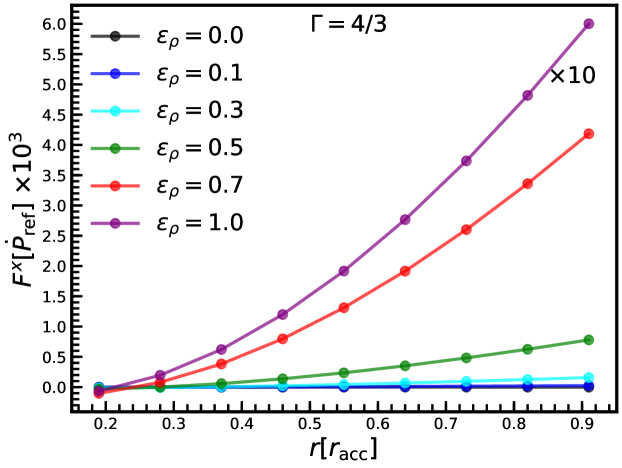
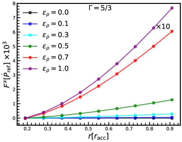
Figure 10.— Total drag forces as measured at different spherical surfaces expressed in terms of the accretion radius (see Equation (33)) and computed after the evolution has reached a stationary state, i.e., for $t>20t_{\rm cross}$. The left and right panels refer to $\Gamma=4/3$ and $\Gamma=5/3$, respectively.

The simple dependence of the total drag force from the density gradient allows us to describe all of the simulation data in terms of a simple phenomenological expression,

$$F^{x}(r,\epsilon_{\rho})=\dot{P}_{\rm ref}\left(\omega_{1}(r)+\omega_{2}(r)\epsilon_{\rho}+\omega_{2}(r)\epsilon^{2}_{\rho}\right)\,,$$ (36)

where $\dot{P}_{\rm ref}$ is the reference linear momentum rate given in Eq. (25) and the coefficients $\omega_{i}(r)$ are reported in Table 3 for $r=r_{{}_{\rm EH}}$ and $r=r_{\rm acc}$. Note that although the Newtonian total drag force has the same functional dependence as in expression (36), the values of the coefficients are rather different (MacLeod & Ramirez-Ruiz, 2015a).

The left panel of the Fig.11 reports the function $F^{x}$ at the event horizon as function of the density gradient and for the two adiabatic indices, with the dotted lines referring to the analytic expression (36).

Table 3Dimensionless units coefficients $\omega_{i}$ total force in the $x$-direction, direction of the black hole’s motion given by equation (36) measured at event horizon and at the accretion radius $r_{\rm acc}$.

$\Gamma$	$\omega_{1}$	$\omega_{2}$	$\omega_{3}$	$\ell_{1}$	$\ell_{2}$	$\ell_{3}$
		$r\sim r_{{}_{\rm EH}}$
$4/3$	$0.54$	$5.79$	$1.02$	$0.542$	$-0.798$	$0.377$
$5/3$	$0.83$	$5.46$	$1.36$	$0.553$	$-0.819$	$0.387$
		$r\sim r_{\rm acc}$
$4/3$	$2.44$	$8.39$	$0.15$	$-$	$-$	$-$
$5/3$	$2.69$	$9.62$	$-1.14$	$-$	$-$	$-$

As mentioned in Sec. 3.1 and as shown in the schematic diagram shown in Figure 1, the presence of a density gradient leads to a deviation of the axis of the shock cone away from asymptotic direction of motion of the fluid. Furthermore, the angle measuring this deviation increases nonlinearly with the density gradient, becoming even larger than $\pi/2$ for $\epsilon_{\rho}=1$. Measuring this angle is important, as it can be used to quantify the deviation of the black hole’s orbit away from a quasi-circular orbit.

Using the data in our simulations once the matter flow has reached a stationary configuration, we can measure this drag angle $\phi_{\rm drag}$ and we have reported the corresponding values as a function of $\epsilon_{\rho}$ in the middle panel of Fig. 11. The simple functional behavior allows us to express the results of the numerical simulations in terms of the simple fitting function (shown as a dotted line in the middle panel of Fig. 11)

$$\phi_{\rm drag}={\cal Q}\,\epsilon^{5/8}_{\rho}\,,$$ (37)

where the constant ${\cal Q}=2.761$ for all models considered here. Interestingly, expression (37) appears “universal” in the sense that it depends only very weakly on the adiabatic index of the envelope.

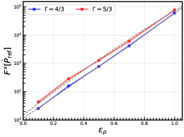
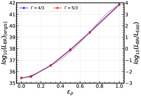
Figure 11.— Left panel: Drag force as a function of the dimensionless density gradient. All positive forces measured at accretion radius $r_{\rm acc}$ are plotted with corresponding fit function given in Eq. ( 36 ). Middle panel: Drag angle between $x$-axis and the shock-cone axis as produced by the density gradients in the envelope. This angle is related to the deviation of the trajectories of the black hole, modifying the orbit of the binary system. Right panel: bremsstrahlung luminosity from interaction of the black hole with a supergiant-star envelope expressed both in $\rm{erg\,s^{-1}}$ and in terms of the Eddington luminosity $L_{\rm Edd}$.

We conclude this Section by considering what could be the radiative signatures of the accretion processes considered here. While we do not have the ambition of performing accurate general relativistic, radiative transfer calculations as those performed by (Zanotti et al., 2011; Roedig et al., 2012) or (Fragile et al., 2014), it is useful to provide here a rough estimate of the luminosity produced considering bremsstrahlung processes from electron–proton collisions (Rybicki & Lightman, 1986; Zanotti et al., 2010)

$$L_{{}_{\rm BR}} = 3.0\times 10^{78}\int\left(T^{\frac{1}{2}}\rho^{2}\sqrt{\gamma}dV\right)\left(\frac{M_{\odot}}{M}\right)\ {\rm\frac{erg}{s}}\,,$$ (38)

which can be readily computed in terms of the quantities evolved in the simulations.

The right panel of Fig. 11 summarizes the results of the simulations as a function of the density gradient and shows that – as expected – the bremsstrahlung luminosity grows with the density gradient and almost exponentially for large gradients. The simple functional behavior of $L_{{}_{\rm BR}}$, which is also essentially independent of the adiabatic index, allows for a simple fitting expression of the type

$$\log\left(\frac{L_{{}_{\rm BR}}}{L_{\odot}}\right)=\frac{1}{\ell_{1}+\ell_{2}\epsilon_{\rho}+\ell_{3}\epsilon^{2}_{\rho}}\,,$$ (39)

where the values of $\ell_{i}$ can be found in Table 3 and the analytic behavior is shown as a dotted line in the right panel of Fig. 11.

4. Conclusions

Using general relativistic simulations, we have carried out a systematic investigation of the properties of the accretion flow onto a nonrotating black hole moving supersonically in a medium with regular but different density gradients. This scenario has been here considered with the goal of providing more accurate and realistic estimates of the secular behavior of the mass accretion and drag rates in the “common-envelope” scenario encountered when a compact object – a black hole or a neutron star – moves in the stellar envelope of a red supergiant star.

The simulations reveal that the supersonic motion always rapidly reaches a stationary state and it produces a shock cone in the downstream part of the flow. At the same time, the gradual change in the density gradient leads to a smooth change general behavior of the flow and in all of the relevant accretion rates. In particular, in the absence of density gradients (i.e., $\epsilon_{\rho}=0$), we recover the phenomenology already observed in the well-known Bondi–Hoyle–Lyttleton accretion problem, with a shock cone and whose axis is stably aligned with the direction of motion (Font et al., 1999; Dönmez et al., 2011; Cruz-Osorio et al., 2012). However, as the density gradient is increased and the black hole encounters a nonuniform medium, the system reaches a steady state where the flow and its discontinuities have found a new equilibrium. When such a state is found – which requires longer times for large density gradients – the shock cone is progressively and stably dragged toward the direction of motion. With sufficiently large gradients, the shock-cone axis can become orthogonal to the direction, or even move in the upstream region of the flow in the case of the largest density gradient (i.e., $\epsilon_{\rho}=1$). In all cases considered – which refer to fluids with adiabatic index set to $\Gamma=4/3$ or $5/3$ – the shock cone heats up the fluid, increasing the temperature by about one order of magnitude with respect to the rest of the envelope, and of almost two orders of magnitude hotter than in the initial state. The fluid is also compressed by the shock, reaching rest-mass densities that are about two orders of magnitude larger than in the unperturbed fluid.

Together with the phenomenological aspects of the accretion flow, we have also investigated and quantified the rates of accretion of mass and momentum onto the black hole, which are particularly important because they ultimately play a leading role in the secular evolution and modeling of the common-envelope scenario. More specifically, and as may have been expected, the rates of accretion of mass and momentum (either radial or angular) increase with the density gradient. Furthermore, this increase becomes essentially exponential as soon as the dimensionless density gradient is $\epsilon_{\rho}\gtrsim 0.2$, thus allowing us to derive simple phenomenological expressions for the mass accretion rate and the momentum accretion rate. Equally simple analytic expressions have been found for the total drag force – which is a combination of the drag due to due the accretion of linear momentum and of the drag due to dynamical friction – of the drag angle of the shock cone and of the bremsstrahlung luminosity that has been estimated. All of these expressions can be readily employed in the astrophysical modeling of the long-term evolution of a binary system experiencing a common-envelope evolution. Furthermore, since the mass accretion rates measured in nonuniform media are well above the Eddington limit, this increases the chances of observing this process also in binary systems of stellar-mass black holes (Caputo et al., 2020).

Finally, we have carried out a systematic comparison with previous Newtonian results, finding that while the general relativistic phenomenology and rates are comparable in the case of the Bondi–Hoyle–Lyttleton scenario (i.e., for $\epsilon_{\rho}=0$), significant differences develop for nonzero density gradients. More specifically, while in a general relativistic context the rates increase with the density gradient, the opposite is true for calculations performed in a Newtonian framework (MacLeod & Ramirez-Ruiz, 2015a). The robustness of the increase of the rates with $\epsilon_{\rho}$ within a relativistic framework has been validated by performing the same simulations with an independent general relativistic MHD code, obtaining results that differ by less than $5\%$.

This different behavior may be due to the different relative strength of gravitational forces in the two contexts, but it may also be due to the different boundary conditions, which we impose inside the event horizon by using the ingoing Eddington–Finkelstein coordinates and are those of a purely infalling gas. On the other hand, the Newtonian framework requires the introduction of a “sink” surrounding the central point mass and whose gravitational potential is smoothed within this sink. The different physical conditions near the black hole (or sink in the Newtonian framework) may also be responsible for the lack of a turbulent flow and vorticity in our simulations, which instead appear in the Newtonian simulations.

The results presented here can be improved in a number of ways. First, we can consider more realistic black holes with nonzero spin; while the spin of black holes in such binary system is currently unknown, determining the dependence of the accretion rates on the black hole spin is of great importance. Second, we can include the contribution of a radiation field – which is expected to decrease but not suppress the mass accretion rate (Zanotti et al., 2011) – by solving, together with the relativistic hydrodynamic equations, also those of relativistic radiative transfer. Finally, we can account for the presence of magnetic fields, which may alter the dynamics of the flow and hence the various accretion rates. We plan to address these additional aspects of the general relativistic common-envelope problem in future works.

Appendix A A. Additional astrophysical considerations

A.1. A.1. Inspiral timescales and different initial data

Following MacLeod & Ramirez-Ruiz (2015b), in this appendix we estimate the inspiral timescale as a function of the density gradients $\epsilon_{\rho}$ and of the accretion rates measured in our simulations. In particular, we define the inspiral timescale as (MacLeod & Ramirez-Ruiz, 2015b)

$$\tau_{\rm insp}:=\frac{E_{\rm orb}}{\dot{E}_{\rm acc}}\,,$$ (A1)

where $E_{\rm orb}$ is the orbital energy that, for a binary system of masses $M$ and $M_{\rm star}$, and separation $a$, is given by (for clarity, we restore the use of the gravitational constant and of the speed of light)

$$E_{\rm orb}:=\frac{M\,M_{\rm star}}{2a}\,.$$ (A2)

On the other hand, $\dot{E}_{\rm acc}$ is the rate of dissipation of the kinetic energy via accretion, which we express in terms of the measured accretion rates and asymptotic velocity as

$$\dot{E}_{\rm acc}=\dot{M}v_{\infty}^{2}\,,$$ (A3)

where the accretion rates are those reported in Fig. 6.

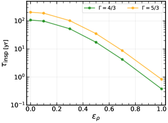
Figure 12.— Inspiral timescale (see Equation (A1)) as function of the dimensionless density gradients $\epsilon_{\rho}$ and the two equations of state considered. The initial separation is assumed to be $a=R_{\rm star}$ and the mass accretion rates are those reported in Fig. 6.

To fix numbers, we evaluate the inspiral timescale after setting $M_{\rm star}=16M_{\odot}$ and $M=4M_{\odot}$ and, as in the rest of the paper, $v_{\infty}=0.2\,c$. The results are shown in Fig. 12, which reports the inspiral timescale for an initial separation of $a=R_{\rm star}$, i.e., when the black hole is just on the outer parts of the common envelope, thus representing the upper limit for the timescale. Under these conditions, and using the accretion rates reported in Fig. 6, we found that the $\tau_{\rm insp}$ $\sim 100\,(200){\rm yr}$ for $\Gamma=4/3\,(5/3)$ and for motion in a uniform medium ($\epsilon_{\rho}=0$). Such timescale decreases by about two orders of magnitude when the considering larger gradients in density. In the extreme case of $\epsilon_{\rho}=1$, the inspiral timescale is as short as $\sim 0.4\,(0.8)\,{\rm yr}$.

A.2. A.2. Impact of the initial data

It is clear that the precise values of the accretion rates ultimately depend on the initial conditions considered, since at the end what matters in determining the mass accretion rate is the size of the mass current near the black hole horizon. In order to investigate a different set of initial conditions, we have carried out simulations employing the initial conditions used in Zanotti et al. (2011), i.e., $v_{\infty}=0.1$ and $c_{s,\infty}=0.07$, thus yielding a Newtonian Mach number $\mathcal{M}_{\infty}\simeq 1.4$. Such a configuration should be contrasted with the reference configuration discussed in the main text, for which $v_{\infty}=0.2$, $c_{s,\infty}=0.1$, and thus $\mathcal{M}_{\infty}=2.0$. In essence, the initial conditions in Zanotti et al. (2011) refer to slower and more tenuous fluid, but also to a flow with a larger accretion radius, i.e., $r_{\rm acc}\simeq 67\,M$ instead of $r_{\rm acc}\simeq 20\,M$. As a result, the computational domain – whose radial extent is set to be $r_{\rm max}=10\,r_{\rm acc}$ – needs to be increased by almost of a factor of three, with a consequent increase in the computational costs.

The results of this investigation for five different values of the dimensionless density gradient are reported in Fig. 13, which is very similar to Fig. 7, but where we also show the accretion rate when considering the initial flow discussed in Zanotti et al. (2011) (purple line) for an adiabatic index $\Gamma=5/3$. Note that despite that fluid is in this case less dense and with a smaller initial velocity, the accretion rate is actually larger because the fluid can be compressed more and this leads to an increase in the mass current near the black hole. While these results highlight that the mass accretion rates also depend on the initial conditions considered, it is useful to note that the reference fluid conditions adopted in the main text (i.e., $\mathcal{M}_{\infty}=2.0$) provide mass accretion rates smaller than those that would be obtained if a more tenuous gas in the stellar envelope were considered. In turn, because smaller values of $\mathcal{M}_{\infty}$ yield smaller accretion rates, it will be easier to reduce them when switching on the coupling with a radiation fluid as done in Zanotti et al. (2011). A more systematic analysis of the dependence of $\dot{M}$ on $\rho_{\infty}$ and $\mathcal{M}_{\infty}$ will be part of our future work.

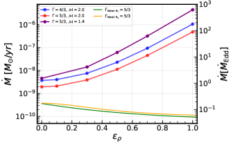
Figure 13.— Same as Fig. 7 but also showing the accretion rate when considering the initial flow discussed in Zanotti et al. (2010) (purple line). Note that despite that fluid is in this case less dense and with a smaller initial velocity, the accretion rate is actually larger because the fluid can be compressed more and this leads to an increase in the mass current near the black hole.

Appendix B B. Additional numerical details

B.1. B.1. Convergence test

The numerical results presented in this work are solving consistently the accretion radius by $200$ cell grids (see Tab. 1), however, in this appendix we also show the convergence test for the model RCE.1.0.5o3 that corresponds to the higher density gradient studied here. For this test, three simulations have been performed using resolutions of $1000\times 128$, $2000\times 256$ (which is also the resolution used for all of the results presented so far) and $4000\times 512$ zones in a uniform grid. Hereafter, we will refer to these resolutions as the low (L), medium (M), and high (H) resolutions.

In particular, we show in the left panel of Fig. 14 the mass accretion rates at different resolutions (top) and the relative differences (bottom) for model RCE.1.0.5o3. Note that the when the flow reaches a steady state, i.e., after $\sim 20$ crossing times, the relative differences are less than $0.1\%$, between both the $\rm H/M$ resolutions and the $\rm M/L$ resolutions. These small differences clearly indicate that the asymptotic rates computed with the M resolution are robust and accurate. The right panel of Fig. 14, on the other hand, reports the differences in the $\mathcal{L}_{1}$ and $\mathcal{L}_{2}$ norms of the rest-mass density at different resolutions, e.g., $\mathcal{L}_{1,L}-\mathcal{L}_{1,M}$, as a function of time. Note that the differences that the differences in the $\mathcal{L}_{1,2}$ norms are of the order of $\sim 10^{-8}$ and $\sim 5\times 10^{-8}$, respectively. Furthermore, using these norms, it is possible to validate that the code is in a convergence regime with convergence order between $1.2$ and $2.0$ (not shown in Fig. 14).

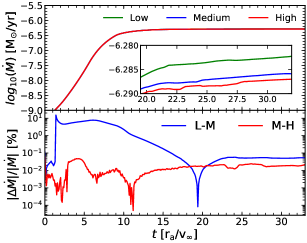
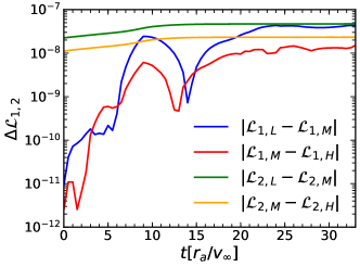
Figure 14.— Left panel: mass accretion rates at the L, M, and H resolutions (top) and the relative differences (bottom) for model RCE.1.0.5o3. The differences between the high resolution and medium (our simulation) are less than $0.1\%$ when the gas reaches to the steady state, as well as when comparing the low and medium resolutions. Right panel: differences in the $\mathcal{L}_{1}$ and $\mathcal{L}_{2}$ norms of the rest-mass density at the three different resolutions.

B.2. B.2. Comparison between BHAC and CAFE

As mentioned in the main text, the numerical results reported in this paper have been produced making use of the CAFE code (Lora-Clavijo et al., 2015a). At the same time, and for the purpose of validating the accuracy of the results – some of which are considerably different from the Newtonian ones – about half of the simulations have also been reproduced by a more recent and advanced numerical code solving the equations of general relativistic MHD: BHAC (Porth et al., 2017). More specifically, all models with adiabatic index $\Gamma=5/3$ have been simulated by both codes for the six values of the density gradient parameter (see Table 1) after using the same numerical methods, grid resolution, and computation domain as described in Section 2.2.

The results of a comparison between the two codes are shown in Fig. 15 for what is arguably the most important quantity among the ones measured: the value of the stationary mass accretion rate as a function of the density parameter. This is shown in Fig. 15, where we show the mass accretion rate in solar masses per year as computed by CAFE (blue line) or by BHAC (red line) for models $\texttt{RCE.0.0.5o3}-\texttt{RCE.1.0.5o3}$. In both cases the mass accretion rate is measured at the event horizon and when a stationary regime in the accretion has been reached, i.e., at $t\sim 5000\,M$. Despite the numerous differences between the two codes, the rates computed are very similar, with differences that are below $5\%$. More importantly, both codes show that the mass accretion rate increases with the density gradient (see Equation (32)), confirming that this is the correct behavior and that the decrease measured in Newtonian calculations is due either to the different strength of the gravitational field or to the different boundary conditions applied at the surface of the compact object.

Figure 15.— mass accretion rate as a function of the density gradient when computed by CAFE (blue line) or by BHAC (red line) for models $\texttt{RCE.0.0.5o3}-\texttt{RCE.1.0.5o3}$. In both cases, the mass accretion rate is measured at the event horizon and when a stationary regime in the accretion has been reached, i.e., at $t\sim 5000\,M$. The relative differences between the two codes are below $5\%$ and both codes report an increase of the mass accretion rate with the density gradient.

References

- Abbott et al. (2016a) Abbott, B. P., Abbott, R., Abbott, T. D., et al. 2016a, Phys. Rev. Lett., 116, 241103
- Abbott et al. (2016b) —. 2016b, Phys. Rev. Lett., 116, 061102
- Alcubierre (2008) Alcubierre, M. 2008, Introduction to Numerical Relativity (Oxford, UK: Oxford University Press)
- Annala et al. (2018) Annala, E., Gorda, T., Kurkela, A., & Vuorinen, A. 2018, Phys. Rev. Lett., 120, 172703
- Armitage & Livio (2000) Armitage, P. J., & Livio, M. 2000, Astrophys. J., 532, 540
- Baiotti & Rezzolla (2017) Baiotti, L., & Rezzolla, L. 2017, Rept. Prog. Phys., 80, 096901
- Banyuls et al. (1997) Banyuls, F., Font, J. A., Ibáñez, J. M., Martí, J. M., & Miralles, J. A. 1997, Astrophys. J., 476, 221
- Barausse (2007) Barausse, E. 2007, Mon. Not. R. Astron. Soc., 382, 826
- Barausse & Rezzolla (2008) Barausse, E., & Rezzolla, L. 2008, Phys. Rev. D, 77, 104027
- Blondin (2013) Blondin, J. M. 2013, Astrophys. J., 767, 135
- Blondin & Pope (2009) Blondin, J. M., & Pope, T. C. 2009, Astrophys. J., 700, 95
- Bodenheimer & Taam (1984) Bodenheimer, P., & Taam, R. E. 1984, Astrophys. J., 280, 771
- Bondi & Hoyle (1944) Bondi, H., & Hoyle, F. 1944, Mon. Not. R. Astron. Soc., 104, 273
- Caputo et al. (2020) Caputo, A., Sberna, L., Toubiana, A., et al. 2020, Astrophys. J., 892, 90
- Clayton et al. (2017) Clayton, M., Podsiadlowski, P., Ivanova, N., & Justham, S. 2017, Monthly Notices of the Royal Astronomical Society, 470, 1788
- Cruz-Osorio & Lora-Clavijo (2016) Cruz-Osorio, A., & Lora-Clavijo, F. D. 2016, Mon. Not. R. Astron. Soc., 460, 3193
- Cruz-Osorio et al. (2012) Cruz-Osorio, A., Lora-Clavijo, F. D., & Guzmán, F. S. 2012, Mon. Not. R. Astron. Soc., 426, 732
- Delgado (1980) Delgado, A. J. 1980, A&A, 87, 343
- Dönmez et al. (2011) Dönmez, O., Zanotti, O., & Rezzolla, L. 2011, Mon. Not. R. Astron. Soc., 412, 1659
- Einfeldt et al. (1991) Einfeldt, B., Roe, P. L., Munz, C. D., & Sjogreen, B. 1991, Journal of Computational Physics, 92, 273
- Faber & Rasio (2012) Faber, J. A., & Rasio, F. A. 2012, Living Rev. Relativity, 15, 8
- Font et al. (1999) Font, J. A., Ibáñez, J. M., & Papadopoulos, P. 1999, Mon. Not. R. Astron. Soc., 305, 920
- Fragile et al. (2014) Fragile, P. C., Olejar, A., & Anninos, P. 2014, Astrophys. J., 796, 22
- Harten et al. (1983) Harten, A., Lax, P. D., & van Leer, B. 1983, SIAM Rev., 25, 35
- Hoyle & Lyttleton (1939) Hoyle, F., & Lyttleton, R. A. 1939, in Proceedings of the Cambridge Philosophical Society, Vol. 35, 405
- Hutilukejiang et al. (2018) Hutilukejiang, B., Zhu, C., Wang, Z., & Lü, G. 2018, Journal of Astrophysics and Astronomy, 39, 21
- Iaconi et al. (2017) Iaconi, R., Reichardt, T., Staff, J., et al. 2017, Monthly Notices of the Royal Astronomical Society, 464, 4028
- Ivanova et al. (2013a) Ivanova, N., Justham, S., Avendano Nandez, J. L., & Lombardi, J. C. 2013a, Science, 339, 433
- Ivanova et al. (2015) Ivanova, N., Justham, S., & Podsiadlowski, P. 2015, Monthly Notices of the Royal Astronomical Society, 447, 2181
- Ivanova et al. (2013b) Ivanova, N., Justham, S., Chen, X., et al. 2013b, Astronomy and Astrophysics Reviews, 21, 59
- Keppens et al. (2012) Keppens, R., Meliani, Z., van Marle, A. J., et al. 2012, Journal of Computational Physics, 231, 718
- Levesque et al. (2014) Levesque, E. M., Massey, P., Żytkow, A. N., & Morrell, N. 2014, Mon. Not. R. Astron. Soc., 443, L94
- Livio & Soker (1988) Livio, M., & Soker, N. 1988, Astrophys. J., 329, 764
- Lora-Clavijo et al. (2015a) Lora-Clavijo, F. D., Cruz-Osorio, A., & Guzmán, F. S. 2015a, Astrophys. J., Supp., 218, 24
- Lora-Clavijo et al. (2015b) Lora-Clavijo, F. D., Cruz-Osorio, A., & Moreno Méndez, E. 2015b, Astrophys. J., Supp., 219, 30
- Lora-Clavijo & Guzmán (2013) Lora-Clavijo, F. D., & Guzmán, F. S. 2013, Mon. Not. R. Astron. Soc., 429, 3144
- Maccarone & de Mink (2016) Maccarone, T. J., & de Mink, S. E. 2016, Mon. Not. R. Astron. Soc., 458, L1
- MacLeod et al. (2017) MacLeod, M., Antoni, A., Murguia-Berthier, A., Macias, P., & Ramirez-Ruiz, E. 2017, Astrophys. J., 838, 56
- MacLeod & Ramirez-Ruiz (2015a) MacLeod, M., & Ramirez-Ruiz, E. 2015a, Astrophys. J., 803, 41
- MacLeod & Ramirez-Ruiz (2015b) —. 2015b, Astrophys. J. Lett., 798, L19
- Margalit & Metzger (2017) Margalit, B., & Metzger, B. D. 2017, Astrophys. J. Lett., 850, L19
- Meyer & Meyer-Hofmeister (1979) Meyer, F., & Meyer-Hofmeister, E. 1979, A&A, 78, 167
- Most et al. (2018) Most, E. R., Weih, L. R., Rezzolla, L., & Schaffner-Bielich, J. 2018, Phys. Rev. Lett., 120, 261103
- Murguia-Berthier et al. (2017) Murguia-Berthier, A., MacLeod, M., Ramirez-Ruiz, E., Antoni, A., & Macias, P. 2017, Astrophys. J., 845, 173
- Nandez & Ivanova (2016) Nandez, J. L. A., & Ivanova, N. 2016, Monthly Notices of the Royal Astronomical Society, 460, 3992
- Nandez et al. (2015) Nandez, J. L. A., Ivanova, N., & Lombardi, Jr, J. C. 2015, Monthly Notices of the Royal Astronomical Society: Letters, 450, L39
- Ohlmann et al. (2016) Ohlmann, S. T., Röpke, F. K., Pakmor, R., & Springel, V. 2016, Astrophys. J. Lett., 816, L9
- Ostriker (1999) Ostriker, E. C. 1999, The Astrophysical Journal, 513, 252
- Paczynski (1976) Paczynski, B. 1976, in IAU Symposium, Vol. 73, Structure and Evolution of Close Binary Systems, ed. P. Eggleton, S. Mitton, & J. Whelan, 75
- Paschalidis et al. (2017) Paschalidis, V., Yagi, K., Alvarez-Castillo, D., Blaschke, D. B., & Sedrakian, A. 2017, Phys. Rev. D, 97, 084038
- Petrich et al. (1989) Petrich, L. I., Shapiro, S. L., Stark, R. F., & Teukolsky, S. A. 1989, Astrophys. J., 336, 313
- Podsiadlowski (2001) Podsiadlowski, P. 2001, in Astronomical Society of the Pacific Conference Series, Vol. 229, Evolution of Binary and Multiple Star Systems, ed. P. Podsiadlowski, S. Rappaport, A. R. King, F. D’Antona, & L. Burderi, 239
- Porth et al. (2017) Porth, O., Olivares, H., Mizuno, Y., et al. 2017, Computational Astrophysics and Cosmology, 4, 1
- Postnov & Yungelson (2014) Postnov, K. A., & Yungelson, L. R. 2014, Living Reviews in Relativity, 17, 3
- Rezzolla et al. (2018) Rezzolla, L., Most, E. R., & Weih, L. R. 2018, Astrophys. J. Lett., 852, L25
- Rezzolla & Zanotti (2013) Rezzolla, L., & Zanotti, O. 2013, Relativistic Hydrodynamics (Oxford, UK: Oxford University Press)
- Ricker & Taam (2012) Ricker, P. M., & Taam, R. E. 2012, Astrophys. J., 746, 74
- Roedig et al. (2012) Roedig, C., Zanotti, O., & Alic, D. 2012, Mon. Not. R. Astron. Soc., 426, 1613
- Ruiz et al. (2018) Ruiz, M., Shapiro, S. L., & Tsokaros, A. 2018, Phys. Rev. D, 97, 021501
- Rybicki & Lightman (1986) Rybicki, G. B., & Lightman, A. P. 1986, Radiative Processes in Astrophysics (Wiley-VCH)
- Shibata et al. (2017) Shibata, M., Fujibayashi, S., Hotokezaka, K., et al. 2017, Phys. Rev. D, 96, 123012
- Shibata & Taniguchi (2011) Shibata, M., & Taniguchi, K. 2011, Living Rev. Relativity, 14, 6
- Shu & Osher (1988) Shu, C. W., & Osher, S. J. 1988, J. Comput. Phys., 77, 439
- Sparks & Stecher (1974) Sparks, W. M., & Stecher, T. P. 1974, Astrophys. J., 188, 149
- Staff et al. (2016) Staff, J. E., De Marco, O., Macdonald, D., et al. 2016, Monthly Notices of the Royal Astronomical Society, 455, 3511
- Taam et al. (1978) Taam, R. E., Bodenheimer, P., & Ostriker, J. P. 1978, Astrophys. J., 222, 269
- Taam & Ricker (2010) Taam, R. E., & Ricker, P. M. 2010, New Astronomy, 54, 65
- Taam & Sandquist (2000) Taam, R. E., & Sandquist, E. L. 2000, ARA&A, 38, 113
- The LIGO Scientific Collaboration & The Virgo Collaboration (2017) The LIGO Scientific Collaboration, & The Virgo Collaboration. 2017, Phys. Rev. Lett., 119, 161101
- The LIGO Scientific Collaboration et al. (2017a) The LIGO Scientific Collaboration, the Virgo Collaboration, Abbott, B. P., et al. 2017a, Phys. Rev. Lett., 118, 221101
- The LIGO Scientific Collaboration et al. (2017b) —. 2017b, Phys. Rev. Lett., 119, 141101
- Thorne & Zytkow (1975) Thorne, K. S., & Zytkow, A. N. 1975, Astrophys. J. Lett., 199, L19
- Zanotti et al. (2010) Zanotti, O., Rezzolla, L., Del Zanna, L., & Palenzuela, C. 2010, Astron. Astrophys., 523, A8
- Zanotti et al. (2011) Zanotti, O., Roedig, C., Rezzolla, L., & Del Zanna, L. 2011, Mon. Not. R. Astron. Soc., 417, 2899