On the development of QPOs in Bondi-Hoyle accretion flows

Abstract

The numerical investigation of Bondi-Hoyle accretion onto a moving black hole has a long history, both in Newtonian and in general-relativistic physics. By performing new two-dimensional and general-relativistic simulations onto a rotating black hole, we point out a novel feature, namely, that quasi-periodic oscillations (QPOs) are naturally produced in the shock cone that develops in the downstream part of the flow. Because the shock cone in the downstream part of the flow acts as a cavity trapping pressure perturbations, modes with frequencies in the integer ratios $2:1$ and $3:1$ are easily produced. The frequencies of these modes depend on the black-hole spin and on the properties of the flow, and scale linearly with the inverse of the black-hole mass. Our results may be relevant for explaining the detection of QPOs in Sagittarius A^∗, once such detection is confirmed by further observations. Finally, we report on the development of the flip-flop instability, which can affect the shock cone under suitable conditions; such an instability has been discussed before in Newtonian simulations but was never found in a relativistic regime.

1 INTRODUCTION

Non-spherical accretion flows are astrophysically relevant in all those situations where strong winds with a small amount of angular momentum are able to transport considerable amounts of matter towards an accreting compact object, e.g., a black hole or a neutron star. Examples include the case of massive X-ray binaries in which a compact object accretes from the wind of an early-type star, or the case of young stellar systems orbiting in the gravitational potential of their birth cluster and accreting from the dense molecular interstellar medium. One of the most celebrated and best studied types of non-spherical accretion flows is the Bondi-Hoyle (Hoyle & Lyttleton, 1939; Bondi & Hoyle, 1944) which, we recall, develops when a black hole moves relative to a uniform gas cloud. The Bondi-Hoyle flow has been the subject of several numerical investigations, starting from Matsuda et al. (1987) and followed by Fryxell & Taam (1988); Sawada et al. (1989); Benensohn et al. (1997). As a summary of the bulk of work done so far on this topic, Table 1 of Foglizzo et al. (2005) reports an overview of published numerical simulations of Bondi-Hoyle-Lyttleton accretion over the last $30$ years and lists more than $40$ works. While providing detailed descriptions of the morphology of the gas capture in the supersonic regime, several of the above mentioned investigations were aimed at verifying the occurrence of the so called flip-flop instability. This consists of an instability to tangential velocities of the shock cone that forms in the downstream region of the flow and it manifests in the oscillation of the shock cone from one side to the other of the accretor.

In the relativistic regime, the first two-dimensional simulations of Bondi-Hoyle accretion were performed by Petrich et al. (1989) and subsequently by Font & Ibáñez (1998b); Font et al. (1998, 1999). These investigations considered flows both in axisymmetry and in the equatorial plane; interestingly none of these works showed the occurrence of the flip-flop instability, so that no evidence existed, prior to this work, about the development of the instability also in a curved spacetime. More recently, a fully general relativistic investigation of the Bondi-Hoyle accretion has been considered by Farris et al. (2010) in the context of the merger of supermassive black-hole binaries; in this case, however, no discussion of the flip-flop instability was presented.

However, the occurrence of the instability is not the only relevant physical process that may manifest in Bondi-Hoyle accretion flows. An additional one, that does not seem to have been considered so far, is related to the possibility that the shock cone traps oscillation modes, thus producing Quasi Periodic Oscillations (QPOs). The intuition is indeed simple yet rather suggestive. The typical shocked cone of the Bondi-Hoyle accretion is likely to provide a natural cavity for the development and confinement of oscillation modes of sonic nature. If the accretor is a compact object, Newtonian hydrodynamics is a good approximation only at large radial distances, while it can lead to misleading conclusions when studying the flow evolution close to the event horizon. In this paper we perform two dimensional general relativistic hydrodynamics simulations by focusing on the dynamical behavior of the Bondi-Hoyle shock cone under a wide range of parameters. The QPOs that we have found have typical frequencies in the range from $10^{-5}$ Hz to $10^{-3}$ Hz for a black hole with $M=10^{6}M_{\odot}$ (and in the range from $1$ Hz to $10^{2}$ Hz for a black hole with $M=10\,M_{\odot}$). As a result, they can become relevant for the interpretation of QPOs observed both in the galactic center and in high-mass X-ray binaries. Our analysis has also shown that the flip-flop instability does occur even in the relativistic framework, and we have investigated how such instability can interplay with the QPO phenomenon, by suppressing or exciting specific modes of oscillations.

The plan of the paper is the following: in Section 2 we provide an overview of the hydrodynamical equations, of the numerical methods adopted and of the physical set up of the problem. In Sec. 3 we describe our results, while Sec. 4 contains a discussion of the potential applicability to two specific astrophysical cases. Finally, Sec. 5 is devoted to the conclusions of our work. We use a geometrized system of units with $G=c=1$.

2 Mathematical formulation

2.1 General relativistic hydrodynamics equations

We study Bondi-Hoyle accretion of a perfect fluid in the curved background spacetime of a rotating black hole. The energy momentum tensor of the fluid has the usual form

$$T^{\mu\nu}=h\rho u^{\mu}u^{\nu}+pg^{\mu\nu}\,,$$ (1)

where $u^{\mu}$ is the four velocity of the fluid, $h$, $\rho$ and $p$ are the specific enthalpy, the rest-mass density and the pressure, respectively. All of these quantities are measured by an observer comoving with $u^{\mu}$, while $g^{\mu\nu}$ is the metric of the spacetime. By adopting the $3+1$ formalism of general relativity and after choosing Boyer-Lindquist coordinates $(t,r,\theta,\phi)$, the line element of the metric is written as

$$ds^{2} = -\left(1-\frac{2Mr}{\Sigma^{2}}\right)dt^{2}-\frac{4Mar}{\Sigma^{2}}\sin^{2}\theta dtd\phi$$

$$+\frac{\Sigma^{2}}{\Delta}dr^{2}+\Sigma^{2}d\theta^{2}+\frac{A}{\Sigma^{2}}\sin^{2}\theta d\phi^{2}\,,$$

where

$$\Sigma^{2} \equiv r^{2}+a^{2}\cos^{2}(\theta)\,,$$ (2)

$$\Delta \equiv r^{2}-2Mr+a^{2}\,,$$ (3)

$$A \equiv (r^{2}+a^{2})^{2}-a^{2}\Delta\sin^{2}\theta\,,$$ (4)

with $a$ and $M$ being the spin and the mass of the black hole. The lapse function and the shift vector of the metric are given, respectively, by $\alpha=(\Sigma^{2}\Delta/A)^{1/2}$ and $\beta^{i}=(0,0,-2Mar/A)$. When solving numerically the general-relativistic hydrodynamic equations it is important to write them in a conservation form (Banyuls et al., 1997)

$$\frac{\partial{\bf{U}}}{\partial t}+\frac{\partial{\bf{F}^{i}}}{\partial q^{i}}={\bf{S}}\,.$$ (5)

where ${\bf{U}}$, ${\bf{F}}^{i}$ and ${\bf{S}}$ are the vectors of the conserved variables, of the fluxes and of the sources, respectively, while $q^{i}$ is the generalized coordinate in the $i-$th direction. When performing two-dimensional numerical simulations in the equatorial plane, Eq.(5) reduces to

$$\frac{\partial{\bf{U}}}{\partial t}+\frac{\partial{\bf{F}}^{r}}{\partial r}+\frac{\partial{\bf{F}}^{\phi}}{\partial\phi}={\bf{S}}\,.$$ (6)

The conservative variables, written in terms of the primitive variables $(\rho,v^{i},p)$, are

$${\mathbf{U}} = \left[\begin{array}[]{c}D\\ S_{r}\\ S_{\phi}\\ \tau\end{array}\right]=\left[\begin{array}[]{c}\sqrt{\gamma}W\rho\\ \sqrt{\gamma}\rho hW^{2}V_{r}\\ \sqrt{\gamma}\rho hW^{2}V_{\phi}\\ \sqrt{\gamma}(\rho hW^{2}-p-W\rho)\end{array}\right]\,,$$ (15)

where $V^{i}=u^{i}/W+\beta^{i}/\alpha$ is a spatial vector whose indices are raised and lowered through the spatial metric $\gamma_{ij}$ and it represents the three-velocity of the fluid with respect to the Eulerian observer associated to the $3+1$ splitting of the metric. $W=(1-\gamma_{ij}V^{i}V^{j})^{-1/2}$ is the Lorentz factor of the fluid and $\gamma={\rm det}(\gamma_{ij})=\Sigma^{4}\sin^{2}\theta/\alpha^{2}$ is the determinant of three metric. Although Font et al. (1999) already reported fluxes and sources for the hydrodynamical equations in the Kerr metric, we explicitly list them here for convenience as

$${\mathbf{F}}^{r} = \left[\begin{array}[]{c}\alpha(V^{r}-\beta^{r}/\alpha)D\\ \alpha\{(V^{r}-\beta^{r}/\alpha)S_{r}+\sqrt{\gamma}p\}\\ \alpha(V^{r}-\beta^{r}/\alpha)S_{\phi}\\ \alpha\{(V^{r}-\beta^{r}/\alpha)\tau+\sqrt{\gamma}V^{r}p\}\end{array}\right]\,,$$ (20)

Table 1: Initial models adopted in numerical simulation. From left to right the columns report: the name of the model, the black hole spin $a$, the asymptotic flow velocity $V_{\infty}$, the asymptotic Mach number ${\cal M}_{\infty}$ and the inner boundary $r_{{\rm in}}$ of the grid. The final simulation time is set equal to $10000M$ in all of the models. The reference adiabatic index adopted is $\Gamma=4/3$, though we have also considered different values to explore the effect on the results.

Model	$a/M$	$V_{\infty}$	${\cal M}_{\infty}$	$r_{{\rm in}}(M)$
$\mathtt{A1}$	$0.9$	$0.001$	$0.01$	$1.78$
$\mathtt{A2}$	$0.9$	$0.1$	$1$	$1.78$
$\mathtt{A3}$	$0.9$	$0.2$	$2$	$1.78$
$\mathtt{A4}$	$0.9$	$0.3$	$3$	$1.78$
$\mathtt{A5}$	$0.9$	$0.4$	$4$	$1.78$
$\mathtt{A6}$	$0.9$	$0.5$	$5$	$1.78$
$\mathtt{A7}$	$0.9$	$0.6$	$6$	$1.78$
$\mathtt{B}$	$0.5$	$0.4$	$4$	$2.1$
$\mathtt{C1}$	$0.0$	$0.001$	$0.01$	$2.1$
$\mathtt{C2}$	$0.0$	$0.1$	$1$	$2.1$
$\mathtt{C3}$	$0.0$	$0.2$	$2$	$2.1$
$\mathtt{C4}$	$0.0$	$0.3$	$3$	$2.1$
$\mathtt{C5}$	$0.0$	$0.4$	$4$	$2.1$
$\mathtt{C6}$	$0.0$	$0.5$	$5$	$2.1$
$\mathtt{C7}$	$0.0$	$0.6$	$6$	$2.1$

$${\mathbf{F}}^{\phi} = \left[\begin{array}[]{c}\alpha(V^{\phi}-\beta^{\phi}/\alpha)D\\ \alpha(V^{\phi}-\beta^{\phi}/\alpha)S_{r}\\ \alpha\{(V^{\phi}-\beta^{\phi}/\alpha)S_{\phi}+\sqrt{\gamma}p\}\\ \alpha\{(V^{\phi}-\beta^{\phi}/\alpha)\tau+\sqrt{\gamma}V^{\phi}p\}\end{array}\right]$$ (25)

and

$${\mathbf{S}} = \left[\begin{array}[]{c}0\\ \alpha\sqrt{\gamma}T^{\mu\nu}g_{\nu\sigma}\Gamma^{\sigma}_{\mu r}\\ \alpha\sqrt{\gamma}T^{\mu\nu}g_{\nu\sigma}\Gamma^{\sigma}_{\mu\phi}\\ \alpha\sqrt{\gamma}(T^{rt}\partial_{r}\alpha-\alpha(T^{rt}\Gamma^{t}_{rt}+T^{rr}\Gamma^{t}_{rr}+T^{r\phi}\Gamma^{t}_{r\phi}))\end{array}\right]$$ (30)

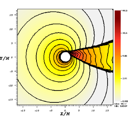
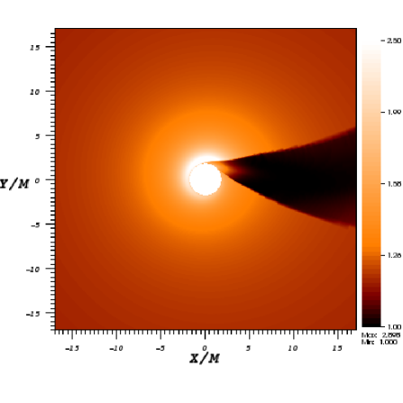
Figure 1: Rest-mass density distribution (left panel) and Lorentz factor distribution (right panel) for a black hole with spin $a=0.9$ and a supersonic flow with asymptotic velocity $V_{\infty}=0.5$, and at time $t=10000\,M$. In the downstream region a clear shock cone forms which is distorted by the non vanishing spin of the black hole.

The equation of state that we adopt is that of an ideal gas, namely

$$p=(\Gamma-1)\rho\epsilon\,,$$ (32)

where $\Gamma$ and $\epsilon$ are the adiabatic index and the specific internal energy, respectively. The reference adiabatic index used in the simulations is $\Gamma=4/3$, though we have also considered different values to explore the effect on the results.

We have solved the system of equations (5) through high-resolution shock-capturing schemes (HRSC) based on approximate Riemann solvers. A minmod linear algorithm for the reconstruction of the left and right states at each interface between adjacent numerical cells is adopted, while the numerical fluxes are computed with the Marquina flux formula. More specific details about the numerical scheme can be found in Dönmez (2004).

As a final remark we note that because we are not here considering any contribution coming from the cooling of the shocked gas, the oscillations we will discuss are not related to those reported by Molteni et al. (1996); Chakrabarti et al. (2004); Okuda et al. (2007). In those studies, in fact, the presence of cooling processes is a necessary ingredient for the appearance of oscillations along the standing shocks.

2.2 Initial Conditions, Boundary Conditions and Approximations

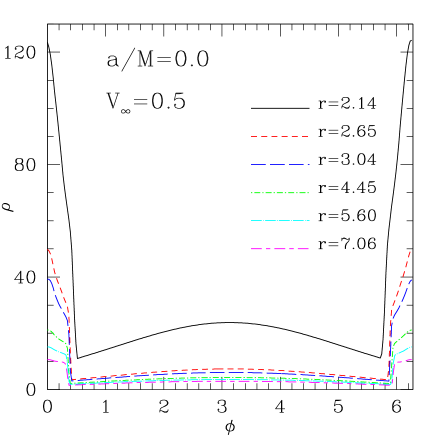
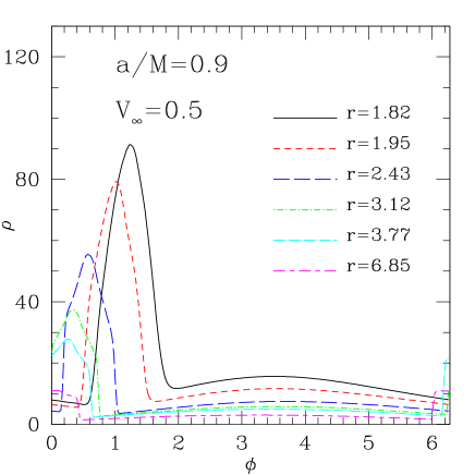
Figure 2: One dimensional profiles of the rest-mass density at time $t=10000\,M$, showing the location of the shock at different radial shells for an asymptotic flow velocity $V_{\infty}=0.5$. The left panel refers to Schwarzschild black hole, while the right one to a rotating black hole with spin $a/M=0.9$. Note that in this latter case the shock is distorted and no longer symmetric.

We perform numerical simulations on the equatorial plane, i.e., $\theta=\pi/2$. The initial velocity field is given in terms of an asymptotic velocity $V_{\infty}$ as in Font et al. (1998), i.e.,

$$V^{r} = \sqrt{\gamma^{rr}}V_{\infty}\cos(\phi)\,,$$ (33)

$$V^{\phi} = -\sqrt{\gamma^{\phi\phi}}V_{\infty}\sin(\phi)\,.$$ (34)

These relations guarantee that the velocity of the injected gas at infinity is parallel to the $x-$direction, while $V^{2}\equiv V_{i}V^{i}=V_{\infty}^{2}$ everywhere in the flow. The value of $V_{\infty}$ can then be chosen to investigate the different regimes of the flow and to consider therefore subsonic or supersonic accretion.

During the evolution additional matter is injected supersonically from the outer boundary in the upstream region with the same analytic prescription of (33) and (34), thus reproducing a continuous wind at large distances. The initial density and pressure profiles are adjusted to make the sound speed equal to a required value, which we choose to be $c_{s,\infty}=0.1$. In practice, once $c_{s,\infty}$ is chosen, we set the density to be a constant (i.e., $\rho=1$) and then the pressure is derived from the relativistic definition of the sound speed, i.e., $p=c^{2}_{s,\infty}\rho(\Gamma-1)/(\Gamma(\Gamma-1)-c^{2}_{s,\infty}\Gamma)$. A brief description of the initial models is reported in Table 1, where models $\mathtt{C*}$ refer to Schwarzschild black holes and different fluid injection velocities, while models $\mathtt{A*}$ and $\mathrm{B}$ refer to Kerr black holes respectively with spin $a/M=0.9$ and $a/M=0.5$, again spanning different fluid injection velocities.

The computational grid consists of $N_{r}\times N_{\phi}$ uniformly spaced zones in the radial and angular directions, respectively, covering a computational domain extending from $r_{\rm{min}}$ (reported in Table 1) to $r_{\rm{max}}=43\,M$ and from $0$ to $2\pi$. For our fiducial simulation we have chosen $N_{r}=512$ and $N_{\phi}=256$, but have also verified that the qualitative results (i.e., the appearance of the QPOs or of the instability) are not sensitive to the resolution used or to the location of the outer boundary, which has been moved to $r_{\rm max}\simeq 80\,M$ in some tests.

The boundary conditions in the radial direction are such that at the inner radial grid point we implement outflow boundary conditions by a simple zeroth-order extrapolation (i.e., a direct copy) of all variables. At the outer radial boundary, on the other hand, we must distinguish between the upstream region, with $\pi/2<\phi<3/2\pi$, and the downstream region, with $-\pi/2<\phi<\pi/2$. In the upstream region we continuously inject matter with the initial velocity field, while in the downstream region we use outflow boundary conditions. Finally, periodic boundary conditions are adopted along the $\phi$ direction.

Finally, we note that in order to validate the code, we have carried out a number of comparisons with the ECHO code presented in Del Zanna et al. (2007), which, among other differences, uses a non-uniform grid structure. The results obtained from the two codes have not shown significant differences.

3 NUMERICAL RESULTS

3.1 Properties of the stationary pattern

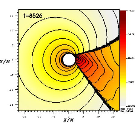
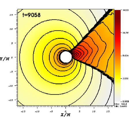
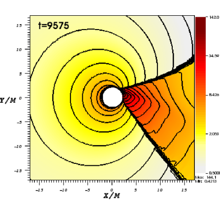
Figure 3: Logarithm of the density at different times for model B with $a/M=0.5$ and $V_{\infty}=0.4$. The flip-flop instability manifests after the shock cone has reached a stationary state and it causes the shock cone to oscillate back and forth with an oscillation period around $1046M$.

The main features of Bondi-Hoyle accretion were first investigated in the relativistic framework through a number of numerical simulations by Petrich et al. (1989); Font & Ibáñez (1998b); Font et al. (1998, 1999). The overall results obtained can be summarized as follows.

As already shown by several authors, when a homogeneous flow of matter moves non radially towards a compact object, a shock wave will form in the neighborhood of the accretor. Depending then on the properties of the flow, namely on the adiabatic index and on the asymptotic Mach number ${\cal M}_{\infty}$, the shock can either reach very close to the accretor or be at a certain distance from it [see, e.g.,  Foglizzo et al. (2005)]. More specifically, for any given value of ${\cal M}_{\infty}$, there is a critical adiabatic index $\Gamma\simeq 2$, below which a shock wave of conic shape, i.e., a “shock cone”, forms in the downstream part of the flow, i.e., downstream of the accretor. Matter from the upstream region crosses continuously the shock front, it undergoes a strong deceleration and, if it is inside the accretion radius, is ultimately accreted. As a result, the maximum rest-mass density in the downstream region is always larger than the corresponding one in the upstream region and, consequently, the mass accretion rate is significantly non-spherical and larger in the downstream part of the flow. Interestingly, when suitable coordinates are used (e.g., Kerr-Schild coordinates), it has been shown by Font et al. (1999) that the shock even penetrates the event horizon. On the other hand, for increasingly stiff fluids and thus for values of the adiabatic index larger than the critical one, a bow shock wave forms in the upstream part of the flow, i.e., upstream of the accretor. In this case the accretion is almost spherical and because the bow shock does not reach into the black-hole’s horizon, it is often referred to as a “detached” shock.

The shape of the shock cone depends sensitively on the spin of the black hole. If the black hole is not spinning, then the shock cone is perfectly symmetric about the $\phi=0$ direction. On the other hand, if the black hole is spinning, the induced frame-dragging effect produces a “wrapping” of the shock cone, as already shown and discussed in great detail by Font et al. (1999).

Our simulations essentially confirm this picture, and the main features of the stationary pattern are summarized in Figure 1, which shows the two dimensional rest-mass density distribution (left panel) and the Lorentz factor distribution (right panel) for model $\mathtt{A6}$ with $a/M=0.9$ and $V_{\infty}=0.5$. As evident from the iso-density contours, the accretion in the upstream region, is essentially spherical accretion, while a very well defined shock cone, characterized by a strong density gradient, forms in the downstream region. The shock cone, where the accretion rate is the largest, is clearly distorted by the spin of the black hole and its opening angle slightly decreases with increasing distance from the center. We have also found that spinning black holes have maximum rest-mass density in the shock cone which is higher than for non spinning black holes. The right panel of Fig. 1, on the other hand, shows that the overall flow is only very mildly relativistic, with a maximum Lorentz factor $W_{\rm{max}}\lesssim 3$, even ahead of the shock front in the vicinity of the black hole. It is also interesting to note that accretion in the shock cone takes place with a very small Lorentz factor. Matter inside the shock cone can accrete onto the black hole only for radii smaller than a given accretion radius $r_{a}$, defined as the radius where the accretion rate (as a function of radius) becomes negative. The expression $r_{a}\approx 2M/(V_{\infty}^{2}+c^{2}_{s,\infty})$, which is valid in the case of a purely-spherical accretion, provides a good estimate of the accretion radius in the Bondi-Hoyle accretion. As an example, for a model with $V_{\infty}=0.5$ and $c_{s,\infty}=0.1$, we found $r_{a}=6.1$, while the predicted one is $r_{a}=7.6$.

To complement the information in Fig. 1, Fig. 2 shows one-dimensional profiles at time $t=10000\,M$ of the rest-mass density at different radial shells for an asymptotic flow velocity $V_{\infty}=0.5$. More specifically, the left panel refers to Schwarzschild black hole, while the right one to a rotating black hole with spin $a/M=0.9$. Clearly, a sharp transition in the density exists at the border of the shock cone and this is particularly evident for the nonrotating black hole. Note also the amount of distortion which is present in the case of a rotating black hole; although this is in part due to our choice of Boyer-Lindquist coordinates, similar distortions are present also when using different and better suited coordinates, such as Kerr-Schild [see the discussion in Font et al. (1999)]. As already mentioned above, the angular location of the shock is only weakly dependent on the radial distance, with the size of the shock cone reducing only slightly when moving away from the black hole. As a final remark we note that the large degree of symmetry shown in the left panel of Fig. 2 provides a convincing evidence of the abilities of the code to maintain the symmetry across $\phi=0$.

3.1.1 The flip-flop instability

As shown through numerical simulations performed by several authors over the years in Newtonian physics, the Bondi-Hoyle accretion flow is subject to the so called flip-flop instability, namely an instability of the shock cone to tangential velocities, which manifests in the oscillation of the shock cone from one side of the accretor to the other. Such instability was first discovered by Matsuda et al. (1987) in 2-D Newtonian axisymmetric simulations, and later confirmed and further investigated by Fryxell & Taam (1988), Sawada et al. (1989), Benensohn et al. (1997), Foglizzo & Ruffert (1999), Pogorelov et al. (2000). Three dimensional simulations were performed by Ishii et al. (1993) and Ruffert (1997), who confirmed the occurrence of the instability, although with deformations of the shock cone only very close the accretor. In spite of all these investigations, however, the nature and the physical origin of the flip-flop instability remain obscure. According to Foglizzo & Ruffert (1999), for example, local instabilities, such as the Rayleigh-Taylor or the Kelvin-Helmholtz instabilities, should not play a significant role and cannot account for the flip-flop instability. On the other hand, Soker (1990) showed, through a WKB analysis, that the two-dimensional axisymmetric accretion flow (not the one considered in our work) can be unstable against tangential modes, as well as against radial modes. When extending these results to three-dimensional simulations, however, the persistence of such instabilities is not fully clarified. Overall, it is fair to say that, although the flip-flop instability has been confirmed numerically both in two and three-dimensional simulations, it is still unclear whether the physical mechanisms driving the instabilities in the two cases are the same or not. Finally, to further complicate the scenario, no evidence was found by Font et al. (1998) of such instability within a relativistic framework, although the authors argued that an instability might develop for very large values of the asymptotic Mach number.

More recently, Foglizzo et al. (2005) performed a very detailed analysis of the unstable behavior of Bondi-Hoyle accretion flows, suggesting that the instability may be of advective-acoustic nature, both in the case of shocks attached or detached (bow shocks) to the accretor. Moreover, they also stressed that, though physical, the instability is likely to be triggered or dumped by numerical effects such as the carbuncle phenomenon at the shock, the boundary condition at the surface of the accretor and the grid size.

Although a detailed analysis of the flip-flop instability is beyond the scope of this paper, which is rather focused on the development of QPOs in Bondi-Hoyle accretion flows, our simulations confirm for the first time the occurrence of the instability even in a relativistic regime. Fig. 3, for instance, reports four snapshots of the rest-mass density in a long term evolution of a model when the instability is fully developed. The shock cone in the downstream region oscillates back and forth in the orbital plane in this representative model with black hole spin $a/M=0.5$ and $V_{\infty}=0.4$. The reason why such unstable behaviour was not noticed by Font et al. (1999) may be due to the short term evolution that they were forced to consider at the time, or, as suggested by Foglizzo et al. (2005), because of the high values of $2M/r_{a}=(V_{\infty}^{2}+c^{2}_{s,\infty})$ that they considered.

Fig. 4 shows additional key features of the flip-flop instability. The top panel, in particular, reports the shock opening angle, as a function of the asymptotic velocity, computed in radians at $r=4.43\,M$ and $t=10000\,M$. Shown with different lines are the values for a Schwarzschild black hole (red solid line) and for a Kerr black hole (blue dashed line). The points with $V_{\infty}=0.3$ and $V_{\infty}=0.4$ correspond to models which are flip-flop unstable and they are located close to the local maximum of the shock opening angle. This results confirms what already reported by Livio et al. (1991), namely that the instability manifests when the shock opening angle is larger than a given threshold. Once the instability is fully developed, the mass accretion rate experiences high amplitude oscillations (for any value of the spin considered). This is shown in the bottom panel of Fig. 4, reporting the evolution of the one-dimensional mass accretion rate $\dot{M}$ defined as

$$\dot{M}\equiv-\int_{0}^{2\pi}{\alpha\sqrt{\gamma}\rho W\left(V^{r}-\frac{\beta^{r}}{\alpha}\right)d\phi}\,,$$ (35)

for different choices of $V_{\infty}$; the specific values reported in the figure refer to a shell at $r=6.08\,M$ and a rotating black hole with spin $a/M=0.9$. It is therefore evident that for small values of $V_{\infty}$, both the mass accretion rate and the shock opening angle are increasing functions of $V_{\infty}$. However, the accretion is no longer efficient above a critical value of $V_{\infty}\simeq 0.4$, and any further increase of $V_{\infty}$ causes both the accretion rate and the maximum rest-mass density in the shock cone to decrease.

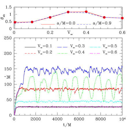
Figure 4: Top panel: shock opening angle in radians as computed at $r=4.43M$, $t=10000\,M$, as a function of $V_{\infty}$. Shown with different lines are the values for a Schwarzschild black hole (red solid line) and for a Kerr black hole (blue dashed line). Bottom panel: time evolution of the mass accretion rate, computed at $r=6.08M$, for different value of $V_{\infty}$ and a rotating black hole with spin $a/M=0.9$. The mass accretion rate manifests high amplitude oscillation in the two flip-flop unstable models with $V_{\infty}\sim 0.3-0.4$.

3.2 QPOs in the shock cone

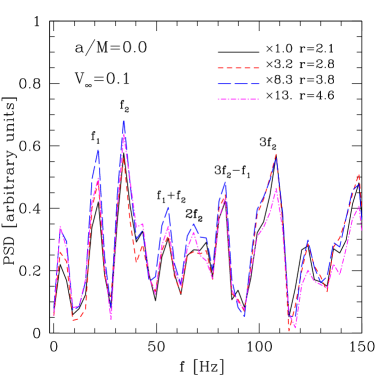
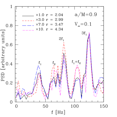
Figure 5: Power spectra of the timeseries of the rest-mass density as computed at the center of shock cone for a flow with asymptotic velocity $V_{\infty}=0.1$. The left and right panels refer to black holes with spins for $a/M=0.0$ and $a/M=0.9$, respectively, while the mass is the same in the two cases and $M=10\,M_{\odot}$. The different curves refer to timeseries recorded at different radial positions but have the same azimuthal position.

As mentioned in the Introduction, one of the most important results presented in this work is about the development of QPOs in the shock cone that forms in the downstream region once the system has relaxed to the stationary state. Note that because a stationary state is necessary for the development of the QPOs, the latter are not found when the flip-flop instability develops. Although the occurrence of QPOs in Bondi-Hoyle accretion has not been discussed before in previous numerical investigations, Fig. 8 of Font & Ibáñez (1998a) does shows a clear periodic behavior of the accretion rate. So, although we can claim to be the first ones to have pointed out the appearance of this effect and to have investigated it in detail, we cannot claim to be the first to have shown found it from numerical simulations.

In order to extract as much information as possible about the emerged phenomenology and provide a first physical explanation, we have carried out an extensive Fourier analysis of the different dynamical quantities. The two panels of Fig. 5, for instance, show the power spectra obtained from the timeseries of the rest-mass density as computed in a region which is in the middle of the shock cone for a flow with asymptotic velocity $V_{\infty}=0.1$. The left and right panels refer to black holes with spins for $a/M=0.0$ and $a/M=0.9$, respectively, while the mass is the same in the two cases and equal to $M=10\,M_{\odot}$. The different curves refer to timeseries recorded at different radial positions but have the same azimuthal position. After performing a series of tests at different resolutions we have estimated the error bar in the measure of each frequency to be $\sim 3{\rm Hz}$.

A number of comments should be made regarding the spectra reported in Fig. 5. The first one is that the modes of oscillation are essentially independent of the radial position, i.e., the power spectra at different radii overlap extremely well. This is a clear indication that the modes are local waves but they are global eigenmodes of the system.

The second comment is that, among the modes reported in Fig. 5, some are genuine eigenmodes, while others are simply the result of nonlinear couplings. In particular, the modes with frequencies $f_{1}=21\,{\rm Hz}$ and $f_{2}=34\,{\rm Hz}$ in the left panel of Fig. 5 are genuine eigenmodes, while those at $55,68,83$ and $106\,{\rm Hz}$ are given, within a few percent error, by nonlinear couplings of the eigenmodes, i.e., $f_{1}+f_{2}$, $2f_{2}$, $3f_{2}-f_{1}$, and $3f_{2}$, respectively. Similarly, the modes $f_{1}=40\ {\rm Hz}$ and $f_{2}=64\,{\rm Hz}$ in the right panel of Fig. 5 are genuine eigenmodes, while the modes at $81,104$ and $124\,{\rm Hz}$ are given, within few percent errors, by $2f_{1}$, $f_{1}+f_{2}$, and $3f_{1}$, respectively. We recall that this behavior is typical of physical systems governed by non linear equations in the limit of small oscillations (Landau & Lifshitz, 1976) and has already been pointed out by Zanotti et al. (2005) in the context of oscillation modes in thick accretion discs around black holes. It should also be remarked that, while a large number of modes due to nonlinear coupling exists, the identification becomes difficult for frequencies larger than $100\,{\rm Hz}$. Similarly, the low-frequency mode at $\sim 5\,{\rm Hz}$, which is visible in both the panels of Fig. 5, could be a genuine mode but it appears with much smaller intensity and not all radii. As a result, its classification as a genuine mode will require more accurate simulations and on much longer timescales.

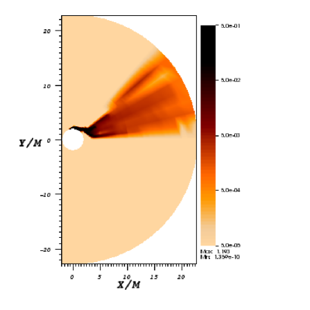
Figure 6: Spatial distribution of the power spectral density at $f=124{\rm Hz}$ for a black hole of mass $M=10\,M_{\odot}$ and spin $a/M=0.9$ (cf. right panel of Fig. 5). A very similar behaviour would be shown in the case of a nonrotating black hole.

The global nature of the oscillation modes inside the shock cone is clearly shown in Fig. 6, which represents the power spectral intensity of the most powerful mode in the right panel of Fig. 5, namely of the mode at $f=124\,{\rm Hz}$ (A very similar behaviour can be seen in the case of a nonrotating black hole.). In other words, for each grid-cell inside the shock cone we store the evolution of the rest-mass density and compute from this the power spectral density. We then consider a single frequency and study how its intensity is distributed (in arbitrary units) inside the shock cone.

Note that the intensity is computed over the whole computational domain, but it has a non-negligible amplitude only inside the shock cone, and this amplitude becomes increasingly stronger near the black hole (We recall that in general we do not expect the amplitude to be constant in the shock cone, as this depends on the specific eigenfunction of the mode). What shown in Fig. 6 is not specific to the mode at $f=124\,{\rm Hz}$ and we have verified that the spatial distribution of the intensity manifests a similar pattern for all of the other modes. Besides providing evidence that these are indeed global oscillation modes of the flow, Fig. 6 also highlights that QPOs can be excited in the shock cone of a Bondi-Hoyle type accretion and that these are particularly stronger close to the black hole.

Interestingly, when the flip-flop instability is triggered and develops, the power spectra inside the shock cone change considerably and in these cases only the periodicity of the shock-cone oscillation can be found, which is then accompanied by the usual nonlinear couplings. In general, therefore, the effect of the flip-flop instability is that of suppressing most of the internal modes of oscillations. A more detailed analysis of this process, as well as of the flip-flop instability will be presented in a future work.

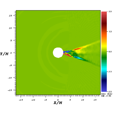
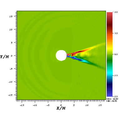
Figure 7: Numerical eigenfunctions computed as $\rho(r,\phi)-{\tilde{\rho}}_{0}(r,\phi)$, where ${\tilde{\rho}}_{0}(r,\phi)$ is the density distribution when the flow is stationary (i.e., for $t\gtrsim 1500\,M$). The left and the right panels report two snapshots at $t=1871M$ and $t=2162M$, and are separated by half a period of oscillation; both refer for to a black hole with spin $a/M=0.0$ and $V_{\infty}=0.1$.

A linear perturbative analysis of the stationary pattern would certainly be of great interest for three important reasons. Firstly, in order to identify unambiguously which of the modes are genuine (or fundamental) and which are the effect of non-linear coupling. Secondly, to compute the expected eigenfrequencies and eigenfunctions of the oscillations we have discovered numerically. Finally to clarify why some modes are more efficiently excited than others. However, such perturbative analysis is probably going to be extremely complicated, mainly because of the absence of an analytic solution for the stationary flow inside the shock cone. To counter these limitations and perform a first rudimentary analysis of the eigenfunctions, we report in Fig. 7 a map of what can be regarded as a numerical eigenfunction for the model $\mathtt{C2}$ ($V_{\infty}=0.1$ and spin $a/M=0.0$). In fact, the two panels of Fig. 7 show the difference $\rho(r,\phi)-{\tilde{\rho}}_{0}(r,\phi)$, where ${\tilde{\rho}}_{0}(r,\phi)$ is the density distribution when the flow is stationary (i.e., for $t\gtrsim 1500\,M$). Considering, for example, the left panel, which corresponds to $t=t_{1}=1871M$ and using Cartesian coordinates, we show in the upper part of the figure, i.e., for $y/M>0$, the density perturbation along the shock is negative close to the black hole, while it is positive far from it. A specular behavior is detected in the lower part of the figure where $y/M<0$. The computed perturbation oscillates in time with a given period $P$, and the right panel of the figure shows a snapshot at time $t_{2}=t_{1}+P/2=2162M$, i.e., at half a period of oscillation. Although heuristic, this procedure allows to compute the period of oscillation of the perturbation with a very good accuracy. The corresponding frequency, again computed assuming $M=10M_{\odot}$, is, in fact, $f\sim 35\,{\rm Hz}$ and it matches very well with the most powerful mode, that with frequency $f_{2}$, reported in the left panel of Fig. 5. To highlight the dependence of the eigenfrequencies on the black hole spin, we report in Table 2 their values as measured within the shock cone from the evolution of the rest-mass density. The mass of the black hole is assumed to be $M=10\,M_{\odot}$, but the frequencies can be easily computed for an arbitrary mass since they scale linearly with the black hole mass. The data in Table 2 suggests that a linear scaling is present also for the black hole spin, but clearly more data is necessary to confirm this scaling, which we will investigate in a future work.

As a final remark we note that, overall, the phenomenology we have found show strong similarities with that reported for perturbed relativistic tori orbiting around a black hole (Zanotti et al., 2003). In that case it was shown by Rezzolla et al. (2003) through a perturbative investigation that the eigenfunctions and eigenfrequencies were those corresponding to the $p$ modes of the torus. Such modes, also known as inertial-acoustic waves, are closely related to the propagation of sound waves in the perturbed fluid and have pressure gradients and centrifugal forces as the main restoring forces. The major difference of the physical conditions investigated by Rezzolla et al. (2003) with the ones considered here is that centrifugal forces play a negligible role in Bondi-Hoyle accretion flows. Apart from this, however, the physical nature of the modes is essentially the same in the two cases. When applied to the oscillations of a thick disc around a compact object, such modes motivated the proposal of a model for explaining the detection of High Frequency Quasi Periodic Oscillations (HFQPOs) in the spectra of X-ray binaries (Rezzolla et al., 2003).

Table 2: Frequencies of the first two genuine modes measured within the shock cone from the evolution of the rest-mass density. The values refer to different black hole spins and different asymptotic velocities, while the mass of the black hole is always assumed to be $M=10\,M_{\odot}$. Note that the frequencies scale linearly with $M$ and the values reported have an error bar of $\sim 3$ Hz.

$a/M$	$V_{\infty}$	$f_{1}$ [Hz]	$f_{2}$ [Hz]
$0.0$	$0.1$	$21$	$34$
$0.5$	$0.1$	$32$	$53$
$0.9$	$0.1$	$40$	$64$
$0.0$	$0.2$	$32$	$46$
$0.9$	$0.2$	$46$	$84$

4 Astrophysical applications

4.1 The case of ${\rm Sgr~{}A}^{\ast}$

A possible application of the results discussed in the previous Section and, in particular, of the development of QPOs in the downstream part of a Bondi-Hoyle flow, is offered by the source Sagittarius A^∗ (or ${\rm Sgr~{}A}^{\ast}$). Such source is located at the centre of our Galaxy and is widely believed to be a supermassive black hole with an estimated mass of $\sim 4.1\pm 0.6\times 10^{6}\,M_{\odot}$ (Ghez et al., 2008; Gillessen et al., 2009). ${\rm Sgr~{}A}^{\ast}$ is one of the most intensely observed astronomical objects and the phenomenology of its emission is both rich and particularly complex. Interestingly, however, QPOs from its emission have been observed by Aschenbach et al. (2004) (see also Aschenbach (2009)), when analyzing two distinct near-infrared and X-ray flares (Genzel et al., 2003). In particular, Aschenbach et al. (2004) reported five different peaks at periods of $100$ s, $219$ s, $700$ s, $1150$ s, and $2250$ s in the power spectral density of such flares. Soon after, Abramowicz et al. (2004) noticed that $(1/700):(1/1150):(1/2250)\approx 3:2:1$, that is, the periods are in a harmonic ratio. Indeed, while discussing the same source, Török (2005) confirmed the measurement of a double peak of QPOs in $\rm{Sgr~{}A}^{\ast}$ in the same typical $3:2$ ratio observed in several low mass X-ray binaries and suggested the epicyclic resonance model by Abramowicz et al. (2003) as a possible explanation for this phenomenology.  Chan et al. (2009), on the other hand, performed two dimensional magnetohydrodynamical simulations of a putative accretion disc in $\rm{Sgr~{}A}^{\ast}$ and showed that the QPOs frequencies could be due to non-axisymmetric density perturbations, and which may be used to set a lower limit on the orbital period at the innermost stable circular orbit.

In addition to QPOs, $\rm{Sgr~{}A}^{\ast}$ is likely to have a Bondi-Hoyle accretion flow. This possibility was first pointed out by Melia (1992), who, after looking at the broad He I, Br$\alpha$ and Br$\gamma$ emission lines, inferred that there is a strong circumnuclear wind near the dynamical center of the Galaxy. In this scenario, the central black hole is assumed to be fed by stellar winds within several arcseconds from the compact object (Shcherbakov & Baganoff, 2010). In order to investigate this possibility further, Ruffert & Melia (1994) performed the first three-dimensional hydrodynamical simulations of this system and computed the line-integrated flux assuming that the emission is dominated by bremsstrahlung. By collecting information coming from more recent observations, Cuadra et al. (2006) and Cuadra & Nayakshin (2006) performed SPH simulations of wind accretion onto $\rm{Sgr~{}A}^{\ast}$, including optically thin radiative cooling and finding, among other results, that most of the accreted gas is hot and has a nearly-stationary accretion rate. Although the observed luminosity is some orders of magnitude smaller than what is predicted by the Bondi-Hoyle model, this may be due to a low radiative efficiency of the accretion flow, rather than to a failure of the Bondi-Hoyle model itself.

Should the two observational features mentioned above be confirmed by additional and more accurate observations, there would be a unique astronomical realization of a source for which both QPOs and Bondi-Hoyle accretion are simultaneously present. It should be stressed that the typical lengthscale at which the QPOs develop in our simulations is $\approx 20\,M$, which thus corresponds to $\approx 4\times 10^{-6}\,{\rm pc}$ for the estimated mass of ${\rm Sgr~{}A}^{\ast}$. This lengthscale is much smaller than the closest approach to the Galactic Center of the closest star S16, which is around $\approx 2\times 10^{-4}{\rm pc}$, as reported by Ghez et al. (2005). Therefore, the Bondi-Hoyle accretion flow that could potentially be present in ${\rm Sgr~{}A}^{\ast}$, would take take place in a gas-dominated region very close to the central black hole and far from the orbits of the S-stars.

Interestingly, after analyzing recent data about a high-level X-ray activity of ${\rm Sgr~{}A}^{\ast}$ observed with XMM-Newton (Porquet et al., 2008; Aschenbach, 2009), Aschenbach (2009) reports nine prominent peaks, named $\nu_{1}\ldots\nu_{9}$. Out of them, only three are identified as fundamental by Aschenbach (2009), namely $\nu_{6}$, $\nu_{7}$ and $\nu_{9}$, while the other six are obtained as linear combinations of the fundamental ones, like, for instance, $\nu_{6}+\nu_{7}$, $\nu_{6}+\nu_{9}$, $\nu_{7}-\nu_{9}$. Aschenbach (2009) interprets the three fundamental modes in terms of orbital, radial epicyclic and vertical epicyclic frequencies. In doing so, a specific radius where the oscillation is excited must be provided, the above osscillation frequencies being intrinsecally local. On the contrary, no radial specification is required within our interpretation, since the modes are global and just confined within the shock cone. Finally, although Aschenbach (2009) does not give any explanation for the other six modes, they are naturally provided within our interpretation of a Bondi-Hoyle accretion in which the downwind shock cone acts as a cavity, generating a whole series of nonlinear couplings among few genuine and trapped pressure modes.

4.2 QPOs in HMXBs

A second application of our result is in principle represented by QPOs observed in the spectra of high mass X-ray binaries (HMXBs), which are composed of a compact object and of an early type (OB) star. The catalog by Liu et al. (2006) lists 114 HMXBs candidates in the Galaxy, some of which are believed to contain a black hole, like Cyg X-1, NGC 5204 (Liu et al., 2004), M 33 X-7 (Pietsch et al., 2004), M 101 ULX-1 (Mukai et al., 2005). Because in these systems the accretion flow occurs preferentially in the form of an accretion wind rather than in the form of an accretion disc, the Bondi-Hoyle accretion flow has been traditionally considered very relevant for them (see the review by Edgar (2004) for the application of the Bondi-Hoyle solution to binary systems). However, the QPOs that have been detected in HMXBs have frequencies that are seen to lie in the range of $1$ mHz to $400$ mHz, with the remarkable exception of XTE J0111.2-7317, which shows a QPO feature at $1.27$  Hz (Kaur et al., 2007). On the other hand, the QPOs we have computed assuming a black hole of mass $M=10\,M_{\odot}$ have frequencies which lie in the range from $1$  Hz to $500$  Hz , and therefore that overlap only marginally with the observed ones.

5 Conclusions

Although viscous accretion discs represent the most natural channel by means of which compact objects accrete large amounts of matter with significant angular momentum, non-spherical accretion flows appear in all those situations in which the accreting matter has only a modest amount of angular momentum, such as in winds. Bondi-Hoyle accretion is the most representative example of this type of flow and its study via numerical investigation has a long history, both in Newtonian and in general-relativistic physics. We have reconsidered this old problem by performing new two-dimensional and general-relativistic simulations onto a rotating black hole. Besides recovering many of the features of this flow which were discussed by other authors over the years, we have also pointed out a novel feature. More specifically, we have shown that under rather generic conditions a shock cone develops in the downstream region of the flow and that such a cone acts like a cavity trapping pressure modes and giving rise to QPOs.

These modes are global in the sense that they represent harmonic oscillations across the cavity, but have amplitudes that are larger in the region very close to the black hole, i.e., for $r\lesssim 10M$. While the black hole spin influences the absolute frequencies of the trapped modes, which lie in the range from $1$  Hz to $500$  Hz for a representative black hole of mass $M=10\,M_{\odot}$, it does not affect the fact that they appear in a series of integer numbers $1:2:3$. This is because nonlinear coupling of modes is common in systems governed by nonlinear equations, and once a mode is excited, all of its integer multiples are also excited, thus producing a wide range of possible ratios of integer numbers.

In addition to pointing out this novel feature of the Bondi-Hoyle accretion, we have discussed its possible application to the phenomenology reported in ${\rm Sgr~{}A}^{\ast}$, where both QPOs (Aschenbach et al., 2004) and Bondi-Hoyle accretion (Melia, 1992) are likely to be present. Remarkably, a large family of linear combinations of modes has been identified recently by Aschenbach (2009) after analyzing data about a high-level X-ray activity of ${\rm Sgr~{}A}^{\ast}$ observed with XMM-Newton (Porquet et al., 2008). This phenomenology could indeed be interpreted in terms of a shock cone that behaves like a cavity and that generates a whole class of nonlinear coupling among pressure modes.

Finally, we have provided the first evidence for the occurrence in a general relativistic context of the so called flip-flop instability of a Bondi-Hoyle flow. More specifically, we have shown that for a fixed choice of the black hole spin and of the sound speed, there exists a critical value of the asymptotic flow velocity at which the shock cone undergoes large-scale and coherent oscillations. When this happens, the opening angle of the shock cone reaches its maximum value, the accretion rate increases considerably and is no longer stationary. A more comprehensive analysis is needed to clarify the physical nature of the instability and its dynamics in the relativistic regime. This will be the focus of a future work.

Finally, among the future improvements of our work we plan to investigate the effects of a magnetic field, which is certainly likely to play a role but whose effective contribution has not been considered yet in numerical simulations of Bondi-Hoyle accretion flows. In particular, the potential interplay of the magnetorotational instability (MRI) with the flip flop instability has to taken into account, though it is not clear whether a local instability such as the MRI can substantially affect a global instability. As far as the occurrence of QPOs, on the other hand, we believe that it will remain essentially unchanged. The reason for this is that as long as a shock cone forms in the downstream part of the flow, QPOs will be naturally excited and trapped, the only difference being that they will be of magnetosonic nature rather than of a sonic one, and hence with eigenfrequencies that will depend not only on the properties of the shock-cone (and thus of the fluid) but also on the strength of the magnetic field.

References

- Abramowicz et al. (2003) Abramowicz M. A., Karas V., Kluzniak W., Lee W. H., Rebusco P., 2003, Pub. Astron. Soc. Japan, 55, 467
- Abramowicz et al. (2004) Abramowicz M. A., Kluźniak W., McClintock J. E., Remillard R. A., 2004, Astrophys. J. Lett., 609, L63
- Aschenbach et al. (2004) Aschenbach B., Grosso N., Porquet D., Predehl P., 2004, Astron. Astrophys., 417, 71
- Aschenbach (2009) Aschenbach B. E., 2009, ArXiv.0911.2431
- Banyuls et al. (1997) Banyuls F., Font J. A., Ibáñez J. M., Martí J. M., Miralles J. A., 1997, Astrophys. J., 476, 221
- Benensohn et al. (1997) Benensohn J. S., Lamb D. Q., Taam R. E., 1997, Astrop. J., 478, 723
- Bondi & Hoyle (1944) Bondi H., Hoyle F., 1944, Mon. Not. R. Astron. Soc., 104, 273
- Chakrabarti et al. (2004) Chakrabarti S. K., Acharyya K., Molteni D., 2004, Astron. Astrophys., 421, 1
- Chan et al. (2009) Chan C.-k., Liu S., Fryer C. L., Psaltis D., Özel F., Rockefeller G., Melia F., 2009, Astrophys. J., 701, 521
- Cuadra & Nayakshin (2006) Cuadra J., Nayakshin S., 2006, Journal of Physics Conference Series, 54, 436
- Cuadra et al. (2006) Cuadra J., Nayakshin S., Springel V., Di Matteo T., 2006, Mon. Not. R. Astron. Soc., 366, 358
- Del Zanna et al. (2007) Del Zanna L., Zanotti O., Bucciantini N., Londrillo P., 2007, Astronomy & Astrophysics, 473, 11
- Dönmez (2004) Dönmez O., 2004, Astrophys. Spac. Sci., 293, 323
- Edgar (2004) Edgar R., 2004, New Astronomy Review, 48, 843
- Farris et al. (2010) Farris B. D., Liu Y. T., Shapiro S. L., 2010, Phys. Rev. D, 81, 084008
- Foglizzo et al. (2005) Foglizzo T., Galletti P., Ruffert M., 2005, Astron. Astrophys., 435, 397
- Foglizzo & Ruffert (1999) Foglizzo T., Ruffert M., 1999, Astron. Astrophys., 347, 901
- Font et al. (1998) Font J. A., Ibáñez J. M. ., Papadopoulos P., 1998, Astrophys. J, 507, L67
- Font et al. (1999) Font J. A., Ibáñez J. M., Papadopoulos P., 1999, Mon. Not. R. Astron. Soc., 305, 920
- Font & Ibáñez (1998a) Font J. A., Ibáñez J. M., 1998a, MNRAS, 298, 835
- Font & Ibáñez (1998b) Font J. A., Ibáñez J. M., 1998b, Astrophys. J., 494, 297
- Fryxell & Taam (1988) Fryxell B. A., Taam R. E., 1988, Astrophys. J., 335, 862
- Genzel et al. (2003) Genzel R., Schödel R., Ott T., Eckart A., Alexander T., Lacombe F., Rouan D., Aschenbach B., 2003, Nature, 425, 934
- Ghez et al. (2005) Ghez A. M., Salim S., Hornstein S. D., Tanner A., Lu J. R., Morris M., Becklin E. E., Duchêne G., 2005, Astrophysical Journal, 620, 744
- Ghez et al. (2008) Ghez A. M., Salim S., Weinberg N. N., Lu J. R., Do T., Dunn J. K., Matthews K., Morris M. R., Yelda S., Becklin E. E., Kremenek T., Milosavljevic M., Naiman J., 2008, Astrophysical Journal, 689, 1044
- Gillessen et al. (2009) Gillessen S., Eisenhauer F., Trippe S., Alexander T., Genzel R., Martins F., Ott T., 2009, Astrophysical Journal, 692, 1075
- Hoyle & Lyttleton (1939) Hoyle F., Lyttleton R. A., 1939, in Proceedings of the Cambridge Philosophical Society Vol. 35, The effect of interstellar matter on climatic variation. pp 405–415
- Ishii et al. (1993) Ishii T., Matsuda T., Shima E., Livio M., Anzer U., Boerner G., 1993, Astrop. J., 404, 706
- Kaur et al. (2007) Kaur R., Paul B., Raichur H., Sagar R., 2007, Astrophys. J., 660, 1409
- Landau & Lifshitz (1976) Landau L. D., Lifshitz E. M., 1976, Mechanics, Volume 1. Pergamon Press, Oxford
- Liu et al. (2004) Liu J., Bregman J. N., Seitzer P., 2004, Astrophys. J., 602, 249
- Liu et al. (2006) Liu Q. Z., van Paradijs J., van den Heuvel E. P. J., 2006, Astron. Astrophys., 455, 1165
- Livio et al. (1991) Livio M., Soker N., Matsuda T., Anzer U., 1991, Mon. Not. Roy. Astr. Soc., 253, 633
- Matsuda et al. (1987) Matsuda T., Inoue M., Sawada K., 1987, Mon. Not. Roy. Astr. Soc., 226, 785
- Melia (1992) Melia F., 1992, Astrophys. J. Lett., 387, L25
- Molteni et al. (1996) Molteni D., Sponholz H., Chakrabarti S. K., 1996, Astrophys. J., 457, 805
- Mukai et al. (2005) Mukai K., Still M., Corbet R. H. D., Kuntz K. D., Barnard R., 2005, Astrop. J., 634, 1085
- Okuda et al. (2007) Okuda T., Teresi V., Molteni D., 2007, Mon. Not. R. Astron. Soc., 377, 1431
- Petrich et al. (1989) Petrich L. I., Shapiro S. L., Stark R. F., Teukolsky S. A., 1989, Astrophys. J., 336, 313
- Pietsch et al. (2004) Pietsch W., Mochejska B. J., Misanovic Z., Haberl F., Ehle M., Trinchieri G., 2004, Astron. Astrophys., 413, 879
- Pogorelov et al. (2000) Pogorelov N. V., Ohsugi Y., Matsuda T., 2000, Mon. Not. R. Astron. Soc., 313, 198
- Porquet et al. (2008) Porquet D., Grosso N., Predehl P., Hasinger G., Yusef-Zadeh F., Aschenbach B., Trap G., Melia F., Warwick R. S., Goldwurm A., Bélanger G., Tanaka Y., Genzel R., Dodds-Eden K., Sakano M., Ferrando P., 2008, Astron. Astrophys., 488, 549
- Rezzolla et al. (2003) Rezzolla L., Yoshida S., Maccarone T. J., Zanotti O., 2003, MNRAS, 344, L37
- Rezzolla et al. (2003) Rezzolla L., Yoshida S., Zanotti O., 2003, MNRAS, 344, 978
- Ruffert (1997) Ruffert M., 1997, Astron. Astrophys., 317, 793
- Ruffert & Melia (1994) Ruffert M., Melia F., 1994, Astron. Astrophys., 288, L29
- Sawada et al. (1989) Sawada K., Matsuda T., Anzer U., Boerner G., Livio M., 1989, Astron. and Astrophys., 221, 263
- Shcherbakov & Baganoff (2010) Shcherbakov R. V., Baganoff F. K., 2010, ApJ, 716, 504
- Soker (1990) Soker N., 1990, Astrop. J., 358, 545
- Török (2005) Török G., 2005, Astron. Astrophys., 440, 1
- Zanotti et al. (2005) Zanotti O., Font J. A., Rezzolla L., Montero P. J., 2005, MNRAS, 356, 1371
- Zanotti et al. (2003) Zanotti O., Rezzolla L., Font J. A., 2003, Mon. Not. Roy. Soc., 341, 832