1 2 1

Microlensing sheds light on the detection of strong lensing gravitational waves

Abstract

The strong lensing gravitational wave (SLGW) is a promising transient phenomenon that encompasses a wealth of physics. However, the long-wave nature of gravitational waves (GW) poses a significant challenge in identification of its host galaxy. To tackle this challenge, we propose a multi-messenger method triggered by the wave optics effect of microlensing. The microlensing diffraction/interference fringes introduce frequency-dependent fluctuations in the waveform. Our method has three steps. First, we reconstruct the GW waveforms by using the template-independent and template-dependent methods. The mismatch of two reconstructions serves as an indicator of SLGWs. This step can identify $10\%$ SLGWs. Second, we pair the SLGW’s multi-signals by employing the sky localization overlapping. Third, we find the host galaxy by requiring the consistency of time delays between Galaxy-Galaxy strong lensing (GGSL) and SLGW. With the help of CSST and JWST, one can identify $1$ quadruple-image system in roughly $3$ years.

Institute for Frontier in Astronomy and Astrophysics, Beijing Normal University, Beijing, 102206, China

Department of Astronomy, Beijing Normal University, Beijing, 100875, China

CAS Key Laboratory of Theoretical Physics, Institute of Theoretical Physics, Chinese Academy of Sciences, P.O. Box 2735, Beijing 100190, China

School of Physical Science and Technology, Ningbo University, Ningbo, 315211, China

In the past $\text{O}1\--\text{O}3$ runs [1, 2, 3], advanced LIGO [4], Virgo [5], and KAGRA [6] (LVK) collaboration have recognized $90$ GW events, including $86$ binary black holes (BBHs), $2$ binary neutron stars (BNSs), and $2$ neutron star–black hole binaries (NSBHs). In the coming years, LVK will continue improving their sensitivity, and LIGO India [7] will join the network in the near future. It is expected that the accumulation of the GW events will rapidly increase with the sensitivity of detectors. Refs. [8, 9] predicted that the lensing detection rate for these upgraded second-generation (2G) detectors is $0.5\--1$ per year, consistent with current non-detection [10, 11, 12, 13, 14, 15]. In contrast, for the third-generation (3G) detectors, such as Einstein Telescope (ET) [16] and Cosmic Explorer (CE) [17], the lensing detection rate will increase to $40\--10^{3}~{}\mathrm{yr}^{-1}$, depending on the population properties of the sources and lenses [18].

The successful detection of SLGW events could facilitate numerous scientific pursuits, such as precision cosmography [19, 20], promoting BBH localization precision [21, 22] and test of general relativity [23, 24, 25], etc. For cosmography, both the time-delay measurement (error of milliseconds level) and the mass reconstruction (free from AGN light contamination) accuracy of SLGWs are much better than those of strong lensed QSOs. Hence, SLGWs can provide more valuable Hubble parameter estimation. For astrophysics, the oscillatory behavior in the waveform as the frequency sweeps up due to wave optics effects can be regarded as a smoking gun for the intermediate-mass black hole [26], a missing piece of cosmic puzzles. However, distinguishing lensing events from a vast unlensed dataset is a formidable challenge. A key issue is to reduce the false alarm rate (FAR).

To the best of our knowledge, four strategies for identification of SLGWs have been proposed in recent years: parameter overlapping [27], machine learning [11, 28], joint-parameter estimation [29, 13, 30], and saddle image analysis with high-order modes [31, 32]. The first two strategies, parameter overlapping and machine learning, exhibit a comparable FAR [28]. They can identify $10\%\--15\%$ lens pairs with a FAR per pair of $10^{-5}$ for $2$G detectors. We extrapolate this detection efficiency to $3$G detectors, assuming that there are $100$ lens pairs and $10^{5}$ unlensed events annually. With this assumption, this method could potentially pick out $10$ to $15$ lens pair candidates along with $50000$ random pairs which are rejected by the null hypotheses (unlensed hypotheses).

Although we may slightly overestimate FAR, we believe that it is not significantly overestimated. The confidence is rooted in the similarity of uncertainties of sky localization between $2$G and $3$G detectors. This distribution ranges from $10^{-2}$ degrees to $10^{4}$ degrees [33], indicating that many random cases with high coincidences will persist. For this reason, Caliskan et al. [34] have argued for the necessity of designing alternative identification criteria beyond the parameter overlapping.

Two possible avenues for such alternatives are proposed. The first involves the incorporation of prior knowledge, including time-delay and magnification ratio between lensing image pairs, as advanced identification criteria. On the one hand, the currently adopted priors are all driven by the data accumulated from the past few decades of strong lensing observations. On the other hand, different priors may lead to different results. For instance, Diego et al. [35] reported two lens pair candidates in the O$3$a catalog by using the prior from the observed distribution of time delays of lensed QSOs [36, 37]. These two candidates were previously rejected by the LVC collaboration [14], utilizing time-delay priors from Singular Isothermal Sphere (SIS) mass model with the velocity dispersion function observed from the Sloan Digital Sky Survey [38] for galaxies and the halo mass function from [39] for clusters. The second avenue centers on employing joint-parameter analysis to enhance identification capabilities. This is the current LVK collaboration adopted method [10, 14, 15]. Compared with the overlapping method, the joint-parameter method is more accurate. Nevertheless, this approach presents a challenge for the future GW detection mission. The computational demands are substantial, with a complexity proportional to $\mathcal{O}(N^{2})$, where $N$ represents the number of GW events.

Therefore, our strategy is to seek a novel search method by exploiting the inherent distinctions in GW signals. Unlike the electromagnetic signals, the GW’s wavelength (at BBH merger phase is about $GM$) is comparable to its source size (about $3GM$). Thanks to this long wave nature of GWs, microlenses (e.g., stars and compact objects) residing in the lens galaxies could leave diffraction or interference imprints on GW’s waveform, which could be treated as a smoking gun for strong lensing events. Ali et al. [40] found that the diffraction induced by a point mass or SIS lens can be identified by using a model-independent method. However, the stochastic nature of the microlensing field poses a formidable challenge in creating a comprehensive template bank capable of effectively filtering these fringes. To address this challenge, we employ a template-free approach, known as the coherent Wave Burst (cWB) [41, 42], to reconstruct the GW waveform. This method is basically looking at the coherent triggers of multi-detectors within the time of flight from one to another. cWB is more suitable for finding the burst signal instead of the long duration one [43]. Compared with BBH merger, BNS merger has long duration. And NSBH merger even do not have the chirp behavior. Hence, in this paper, we focus on the GWs generated by BBH only.

In this study, we will introduce a multi-messenger approach for the identification of SLGWs. Our approach involves the detection of SLGW, the search for pairs of SLGW, and the subsequent identification of the host galaxies associated with these events. This methodology effectively addresses the inherent challenges of traditional methods. The detection of microlensing together with strong lensing provides us an efficient way of searching for SLGWs. Consequently, it will enrich the utility of SLGWs in the realms of astrophysical and cosmological research.

cWB reconstruction We illustrate our result by simulating an SLGW event generated by the BBH merger. We adopt the single-precessing-spin waveform model IMRPhenomPv2 [44, 45] encoded in PyCBC [46] and three CE detectors located at Livingston (USA), Hanford (USA) and Pisa (Italy) to generate the simulated strain data.

To illustrate the lensing effect more visually clear, the macro lensing magnification of this event is chosen as 66 (macro lensing convergence $\kappa\simeq 0.492$, macro lensing shear $\gamma\simeq 0.492$). Furthermore, we conservatively choose the microlensing convergence as $\kappa_{*}=0.09$, which corresponds to $f_{*}\simeq 0.2$ ($\kappa_{*}=f_{*}\kappa$). This $f_{*}$ value is almost the lower bound suggested by Dobler et al. [47].

Following the recipe listed in Refs. [48, 49, 50], we generate the microlensing fields. Then, we use the algorithm introduced in Shan et al. [50] to evaluate the Fresnel-Kirchhoff diffraction integral [51]

$$F(\omega,\bm{y})=\frac{2G\mathrm{M}_{L}\left(1+z_{L}\right)\omega}{\pi c^{3}i}\int_{-\infty}^{\infty}d^{2}x\exp\left[i\omega t(\bm{x},\bm{y})\right]\;,$$ (1)

where $F(\omega,\bm{y})$ is the wave optics magnification factor, $\omega$ and $\bm{y}$ are the circular frequency of the GW and its position in the source plane in the unit of the Einstein radius. $\mathrm{M}_{L}$ and $z_{L}$ are the lens mass and redshift, $\bm{x}$ is the lens plane coordinate, and $t(\bm{x},\bm{y})$ is the time delay function defined as

$$\begin{split}t(\bm{x},\bm{x}^{i},\bm{y}=0)&=\underbrace{\frac{k}{2}\left((1-\kappa+\gamma)x_{1}^{2}+(1-\kappa-\gamma)x_{2}^{2}\right)}_{t_{\text{s}}(\kappa,\gamma,\bm{x})}-\underbrace{\left[\frac{k}{2}\sum_{i}^{N}\ln\left(\bm{x}^{i}-\bm{x}\right)^{2}+k\phi_{-}(\bm{x})\right]}_{t_{\text{m}}(\bm{x},\bm{x}^{i})}\end{split}$$ (2)

where $k=4G\text{M}_{\text{micro}}(1+z_{L})/c^{3}$ and $\bm{x^{i}}$ is coordinate of the $i$th microlens. Here, we set the macro image point as the coordinate origin ($y=0$). $\phi_{-}(\bm{x})$ is the contribution from a negative mass sheet which is used to cancel out the mass contribution from microlenses and keep the total convergence $\kappa$ unchanged [52, 48, 49]. $t_{\text{s}}(\kappa,\gamma,\bm{x})$ represents the macro lens time delay and $t_{\text{m}}(\bm{x},\bm{x}^{i})$ indicates the microlens time delay.

The product of the wave optics magnification factor and the unlensed waveforms $\tilde{h}_{+,\times}(f)$ gives the lensed GW waveform $\tilde{h}^{L}_{+,\times}(f)$ in the frequency domain

$$\tilde{h}^{L}_{+,\times}(f)=F(f)\tilde{h}_{+,\times}(f).$$ (3)

As is shown in the black curve in Figure 1, the microlensing wave optics effect could leave a frequency-dependent imprint on the GW waveform. Currently, while the techniques for searching this feature produced by isolated microlens have matured [10, 14, 40], only a few pioneer works have studied the microlensing field scenario [53, 54, 55]. As we have discussed above, the waveform template of GW intersecting with the stochastic microlensing fields could not be modeled deterministically. So the traditional matched filtering method is no longer suitable for our goal. Fortunately, as shown in Figure 1, these microlensing imprints can be reconstructed using a template-free method, cWB. The blue curve in the upper panel shows the reconstructed GW waveform from cWB. The $x$-axis is the GW frequency, and the $y$-axis is the absolute value of the waveform. One can find that the blue curve is consistent with the black, which is our injected microlensed GW signal. The extra fast oscillations in the blue curve compared with the black is the unwanted instrumental noise. This result demonstrates the robustness of cWB for reconstructing the microlensing effect. Furthermore, we show the best-fit waveform reconstructed from the template fitting using the template without microlensing in the smoothing red curve. The waveform template used in parameter estimation is IMRPhenomPv2 encoded in Bilby [56]. One can find that the Bilby result is very different from the result of cWB, which indicates that the fifteen parameters waveform can not reconstruct the microlensing wave optics effect at all. This result serves to highlight that the spin precessing effect is incapable of reproducing the microlensing diffraction imprint [57]. This distinction arises because the precessing effect unfolds gradually, whereas the microlensing field demonstrates a more random behavior. The lower panel shows the ratio between $\tilde{h}_{\mathrm{cWB}}$ and $\tilde{h}_{\mathrm{Bilby}}$ as the blue curve. Comparing it with the injected value, $F(f)/\sqrt{\mu}$ (black), one can find that Bilby reconstruct the strong lensing waveform with a bit of bias, but cWB can capture the microlensing effects.

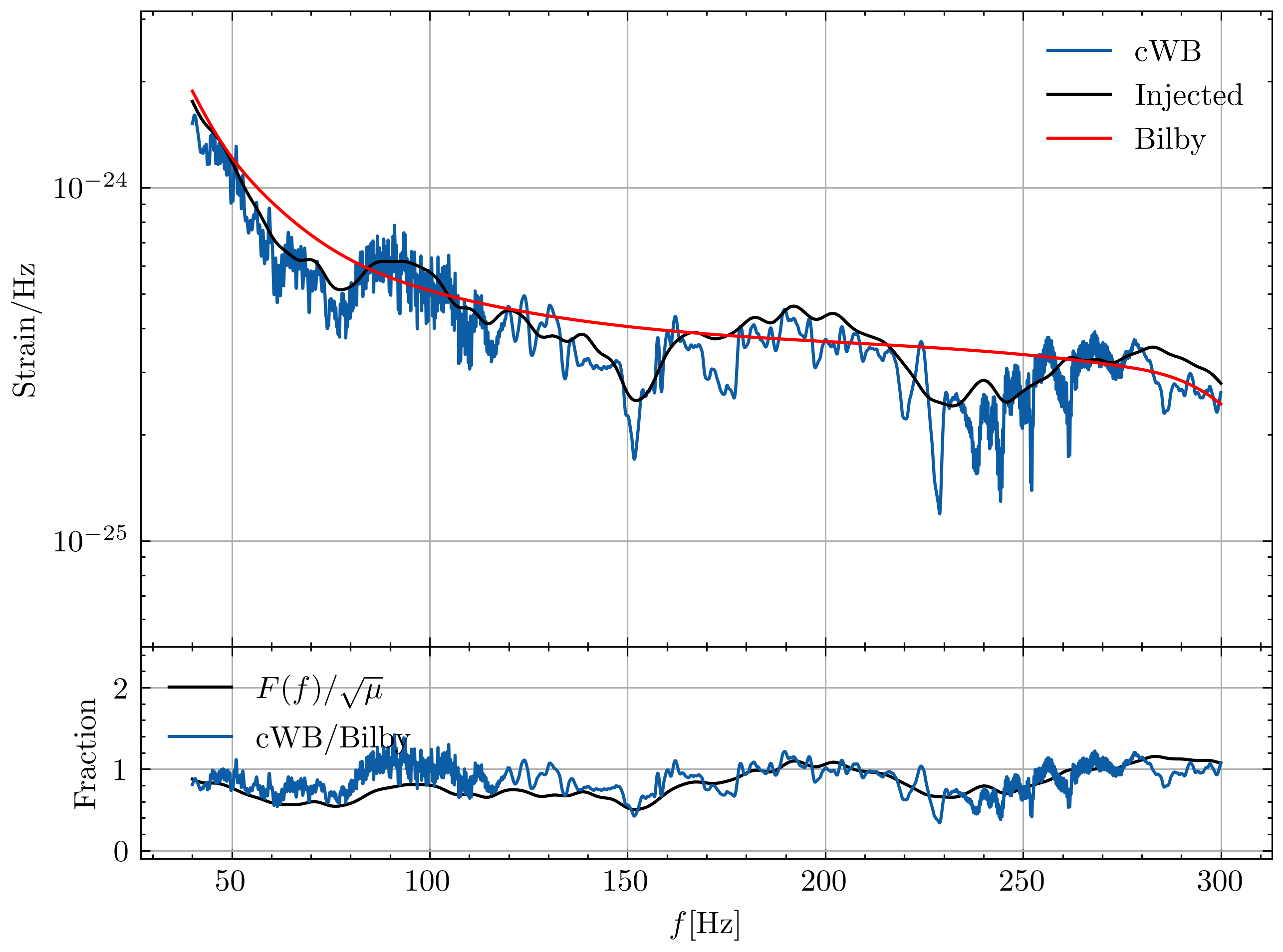
Figure 1: cWB and Bilby reconstruction results. The blue and red curves in the upper panel represent the reconstruction results of cWB and Bilby, respectively. The black curve is the injected GW waveform. The $x$-axis is the GW frequency, and the $y$-axis is the absolute value of the waveform. The blue curve in the lower panel shows the ratio of cWB and Bilby results. The black curve is the injected ratio of the wave optics magnification factor $F(f)$ and the square root of the macro magnification $\sqrt{\mu}$.

Identification of SLGW single-signal In the previous section, we showcases the robustness of cWB in accurately reconstructing the microlensing signature encoded in the SLGW. In this section, we introduce a new method for the authentication of SLGW events. Specifically, our approach involves the evaluation of mismatch between cWB and Bilby outcomes, serving as a means to ascertain the eligibility of a given event as an SLGW event. Here, we define the match equation as

$$\mathrm{match}=\frac{\left\langle\tilde{h}_{\mathrm{cWB}}\mid\tilde{h}_{\mathrm{Bilby}}\right\rangle}{\sqrt{\left\langle\tilde{h}_{\mathrm{cWB}}\mid\tilde{h}_{\mathrm{cWB}}\right\rangle\left\langle\tilde{h}_{\mathrm{Bilby}}\mid\tilde{h}_{\mathrm{Bilby}}\right\rangle}}\;,$$ (4)

where $\tilde{h}_{\mathrm{cWB}}$ and $\tilde{h}_{\mathrm{Bilby}}$ are the reconstructed waveforms in the frequency domain. $\left\langle.\mid.\right\rangle$ stands for the noise-weighted inner product and is defined as

$$\left\langle\tilde{h}_{1}\mid\tilde{h}_{2}\right\rangle=4\operatorname{Re}\int_{f_{\text{low }}}^{f_{\text{high }}}\mathrm{d}f\frac{|\tilde{h}_{1}(f)|\times|\tilde{h}_{2}(f)|}{S_{\mathrm{n}}(f)}\;,$$ (5)

where $|.|$ refers to the absolute value, and $S_{\mathrm{n}}(f)$ is the single-side power spectral density of the detector noise. It is evident that Eq. (4) is $\leq 1$, and the equality holds if and only if $\tilde{h}_{\mathrm{cWB}}=\tilde{h}_{\mathrm{Bilby}}$ (Cauchy-Schwarz inequality). One can imagine that the efficiency of this method depends on the quality of the reconstruction results and the strength of the microlensing imprints. To demonstrate the reliability of the above method, we need to know the FAR, namely, to what extent unlensed events can mimic the result of lensed events. We randomly select $200$ GWs from the unlensed dataset simulated in Sec. Method to construct the false positive sets.

The microlensing field in this study are generated according to the Salpeter initial mass function (IMF) [58] and an elliptical Sésic profile [59] to describe the stellar mass function and density associated with each SLGW. Specifically, we set the stellar mass range to be within $[0.1,1.5]$ solar masses, which aligns with the value employed by Diego et al. [60]. In addition to the stellar mass component, we also consider the presence of remnant objects in the microlensing field. For this purpose, we adopt the initial-final relation (IFR) from Spera et al. [61]. The remnant mass density has been set at $10\%$ of the stellar mass density [55].

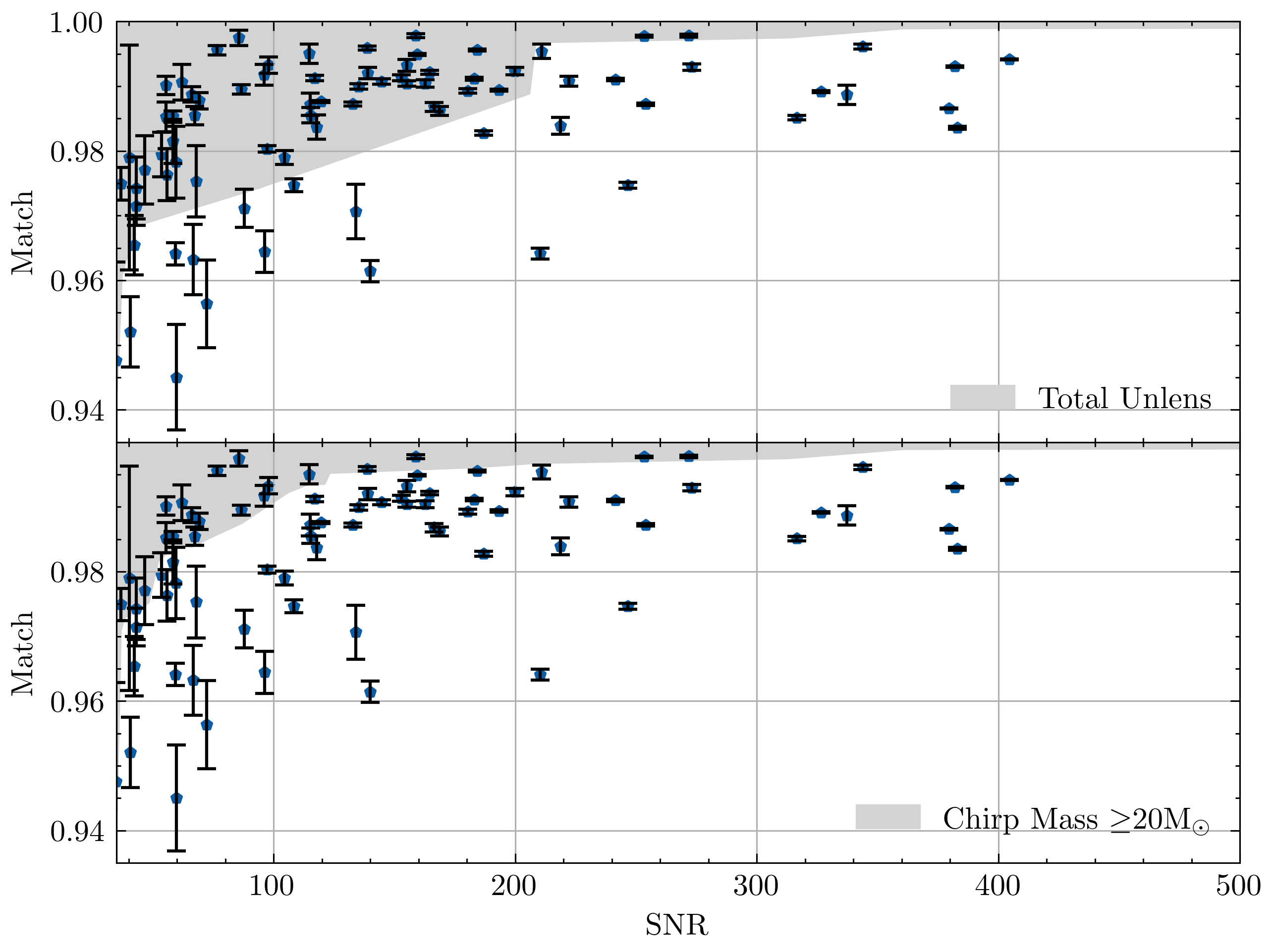
Figure 2: Identification of SLGW events. This figure shows the match result between cWB and Bilby as a function of SNR. The grey shaded areas represent the envelope of the lower matching limit of all unlensed events (false positive samples). The black error bars ($90\%$ confidence interval) with blue pentagrams (mean value) represent the match results of SLGWs. The upper and lower panels show the results without and with detector frame chirp mass $\mathcal{M}_{z}\geq 20M_{\odot}$ cut, respectively.

The grey shaded areas in Figure 2 represent the match result of cWB and Bilby for these false positive samples. The $x$-axis stands for the matched-filter SNR. It is worth mentioning that when calculating the matching for each event, we randomly select $100$ groups of parameter values from the posterior distribution of the Bilby results and match them with the result of cWB. The envelope of the shaded area is the lower matching bound of all false positive events. The upper and lower panels stand for results without and with detector frame chirp mass $\mathcal{M}_{z}=20~{}\mathrm{M}_{\odot}$ cut, respectively. One can find that the match value is proportional to SNR. This result is expected because, at high SNR, both cWB and Bilby can faithfully reconstruct the actual GW waveform with tiny uncertainty. Comparing the two panels demonstrates that $\mathcal{M}_{z}>20~{}\mathrm{M}_{\odot}$ truncation can significantly improve the matching result for events with SNR$\in(40,200)$. We note that setting a cutoff of $\mathcal{M}_{z}=20~{}\mathrm{M}_{\odot}$ is cost-effective. It only loses $\sim 17\%$ SLGWs (after doing a statistic calculation), but can significantly reduce the FAR.

We simulate the GW data for $3$ years and consider the duty circle as $80\%$. The black error bars ($90\%$ confidence interval) with blue pentagrams (mean value) in Figure 2 represent the match results for SLGW events. Within $3$ years, $>58$ signals out of the total of $560$ detectable SLGWs fall outside the shaded region. These selected SLGW events can be confidently confirmed with tiny the risk of false-positive contamination. Conversely, the remaining events exhibit microlensing wave optics effects that are too faint to distinguish successfully from the false positive background. Although an accurate estimation of the FAR will be more convincing, the computational limitation of this work (approximately $1.4\times 10^{5}$ events per year) makes it challenging to provide such an estimation. Nevertheless, we believe that the occurrence of false mismatch events due to random effects is negligible. Random effects are unlikely to mimic such substantial mismatch values, especially at high SNR. Moreover, our research demonstrates that the shaded region’s boundaries remain consistent when comparing estimation results for $100$ GWs and $200$ GWs. Therefore, the results are convergent. Furthermore, it’s worth noting that false positive events are proportional to the total number of GWs, $N$, rather than $N^{2}$. This indicates that our method is less susceptible to random chance than traditional “overlapping” like methods. Taking all these considerations into account, we assert that events falling below the shaded region can confidently be classified as SLGWs events. In summary, our method has the capacity to identify more than $10\%$ of SLGWs annually.

Strong lensing pairing In the preceding section, we successfully authenticated $58$ single-signal SLGW systems on an annual basis. Through an analysis of the parameter overlapping between these $58$ single-signal systems and other GWs, we were able to select the multiple-image pairs associated with these single signals (for more details, please refer to the Method section).

Figure 3 presents the results of our multi-signal identification process. The left $y$-axis represents the FAR per year, while the right $y$-axis represents the FAR per pair. The $x$-axis corresponds to the event index. In this analysis, we chose an FAR per year of $0.01$ to represent events that can be confidently selected. This value indicates that, on average, one hundred years of observations may yield a false pair associated with the identified single-signal. In the figure, we use red stars to highlight the safely identified multi-signal pairs, while grey dots with grey shadows represent pairs that could not be identified. Notably, our analysis identified $22$ double-image systems and $3$ quadruple-image systems (enclosed within the blue box) in $3$ years.

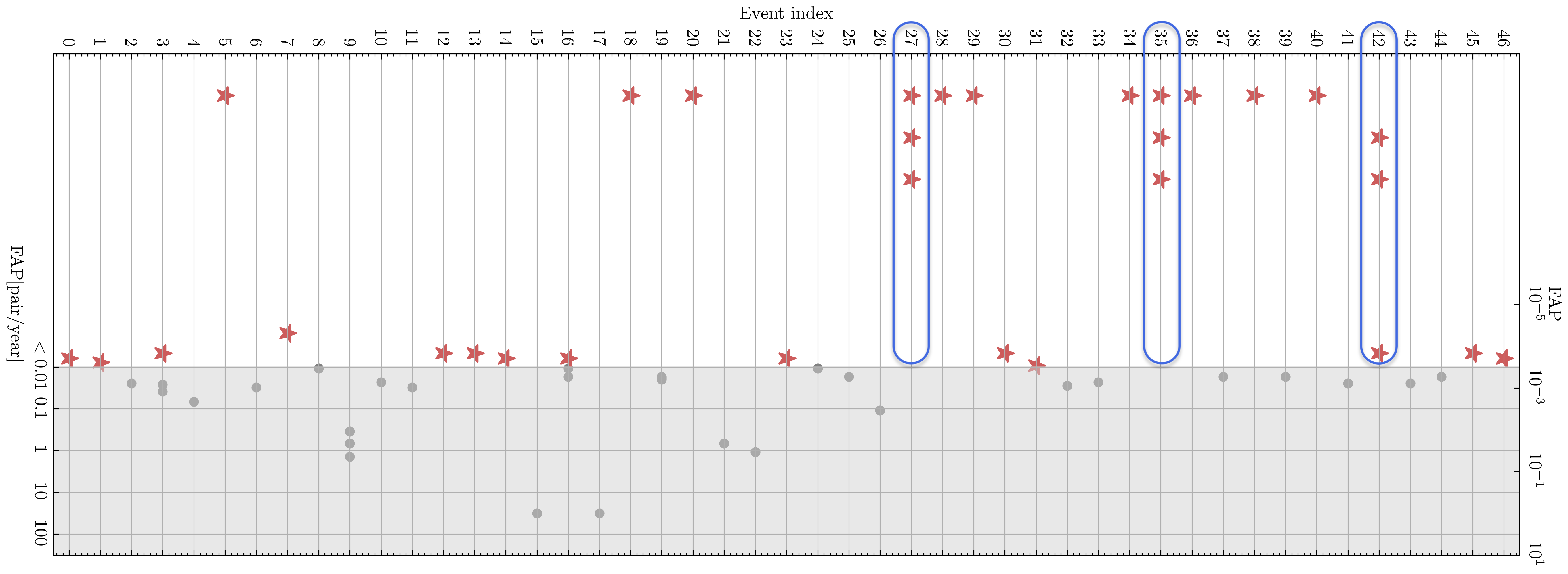
Figure 3: Identification of SLGW pairs. This figure displays the results of finding SLGW pairs. The left $y$-axis represents the FAR per year, while the right $y$-axis represents the FAR per pair. The $x$-axis corresponds to the event index. In the figure, red stars are used to highlight the safely identified multi-pairs, while grey dots with grey shadows represent pairs that could not be identified.

Host galaxy identification In the context of quadruple-image systems, the identification of host galaxies can be accomplished through a comparison between the time delays associated with SLGW and GGSL events, as detailed in Hannuksela et al. [21]. In the GGSL Simulation and Host Galaxy Identification section, we introduce a new time-delay discriminator designed to distinguish host galaxies from unrelated GGSL systems.

Figure 4 showcases the host galaxy identification confidence interval obtained for event ID-35 (Figure 3), acquired using Chinese Survey Space Telescope (CSST) and James Webb Space Telescope (JWST). CSST is used to select the GGSL candidates and JWST is used for a dedicated follow-up. Among the three selected quadruple-image systems discussed in the previous section, the host galaxy of the ID-35 event stands out as the brightest (smallest source redshift, $z_{s}=1.6$), as demonstrated in Supplementary Figure 8 and most accurate sky localization ($1.3$ square degrees). The $y$-axis in Figure 4 represents the reverse cumulative distribution function of the time delay prediction from the GGSL image reconstruction w.r.t. the SLGW measurement. The time delay measurement error from SLGW is the order of milli-second, which can be safely neglected. The blue curve represents unhosted GGSL systems, whereas the red curve signifies host galaxies with varying magnitudes, spectral energy distributions (SED), and light Sésic profiles, all of which are weighted by the Star Formation Rate (SFR). It’s important to note that the blue curve includes all simulated unhosted GGSL systems within an area spanning $20$ square degrees, which is observed by the CSST. This sky region exceeds the sky localization of the specific event under consideration, covering approximately $1$ square degree. Hence, the results presented here are conservative. Within $1$ square degree, one can find around $3$ quadruple-image GGSL candidates in CSST images. Then, we ask for a JWST $1000s$ follow-up for each of these $3$ systems. According to Figure 4, it is evident that we can effectively select the host galaxy out of the unhosted GGSL systems. Furthermore, as shown in the middle panel (ID-35) of Supplementary Figure 8, CSST demonstrates the capability to identify approximately $80\%$ of all potential host galaxies, represented by the ratio between the white and white+grey areas enclosed by the red histogram of ID-35. In conclusion, the probability of successfully identifying the host galaxy for this SLGW event is estimated to be approximately $80\%$.

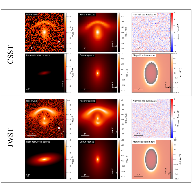
Figure 9: Host galaxy reconstruction. This figure illustrates the GGSL reconstruction for the most likely host galaxy of the SLGW. The first panel (first and second rows) displays the result of CSST, while the second panel (third and fourth rows) shows the results obtained using JWST. For each panel, the first row from left to right includes: The observed image, the reconstructed image and the normalized residuals. The second row for each panel from left to right includes: The reconstructed source light, the convergence and magnification map.

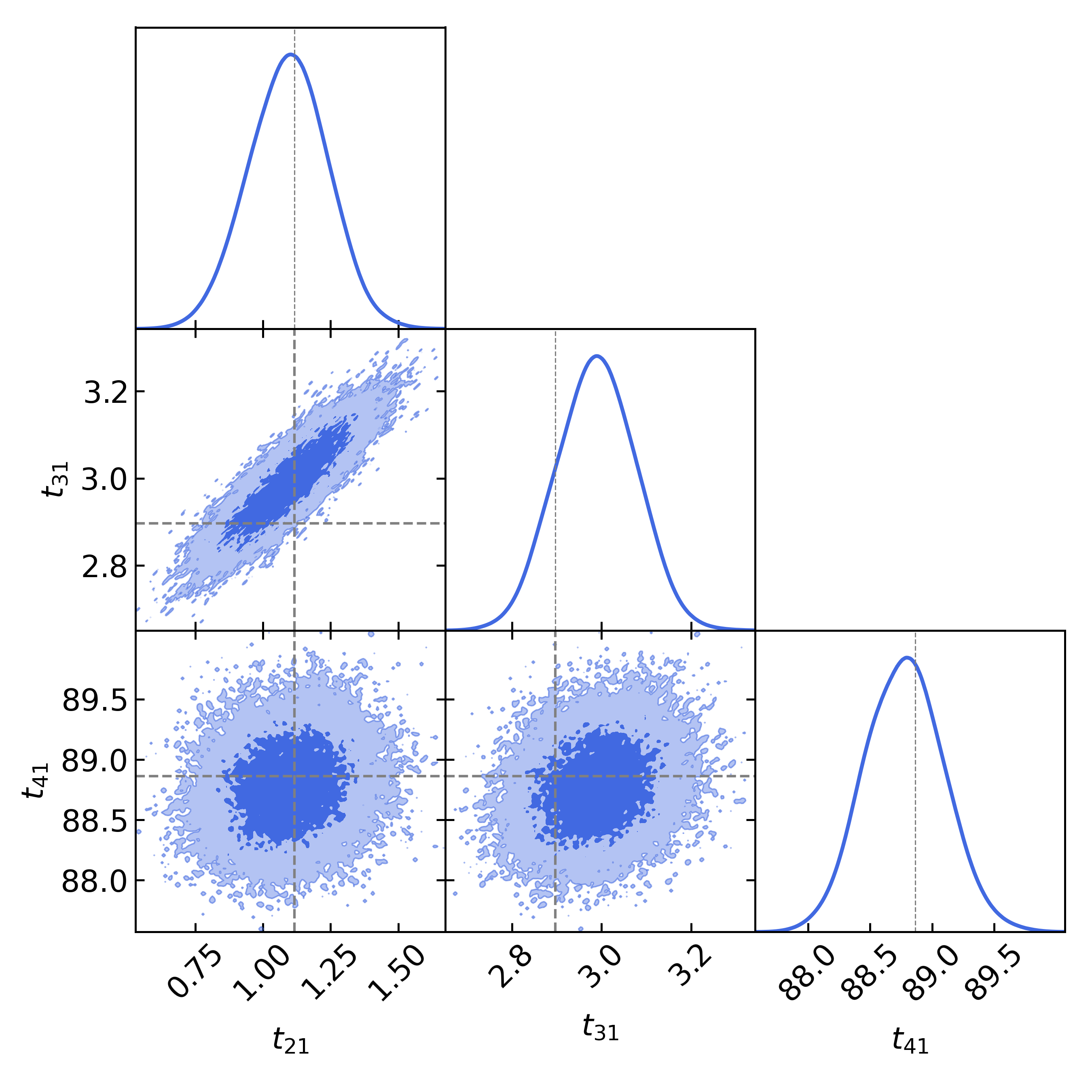
Figure 10: Posterior distribution of time delay. This figure shows the time delay reconstruction result for the most likely host galaxy of the SLGW. The $x$-labels represent the time delay differences for different images pairs in a quadruple-image system.

In Supplementary Figure 9, we present the host galaxy reconstruction for the event ID-35. The host galaxy is assigned with the most probable SFR. The first panel (first and second rows) displays results from CSST (Sloan $r$-band $600s$ exposure), while the second panel (third and fourth rows) shows the results obtained through observations using JWST (F$200$W/$2\mu m$ band $1000s$ exposure). For each panel, the first row from left to right includes: the observed image, the reconstructed image and the normalized residuals. The second row for each panel from left to right includes: the reconstructed source light, the convergence and magnification map. In Supplementary Figure 10, we present the posterior distribution of the time delay from GGSL reconstruction for the most likely host galaxy. Notably, the SLGW time delay data (grey dashed line) falls well within the $3\sigma$ confidence intervals.

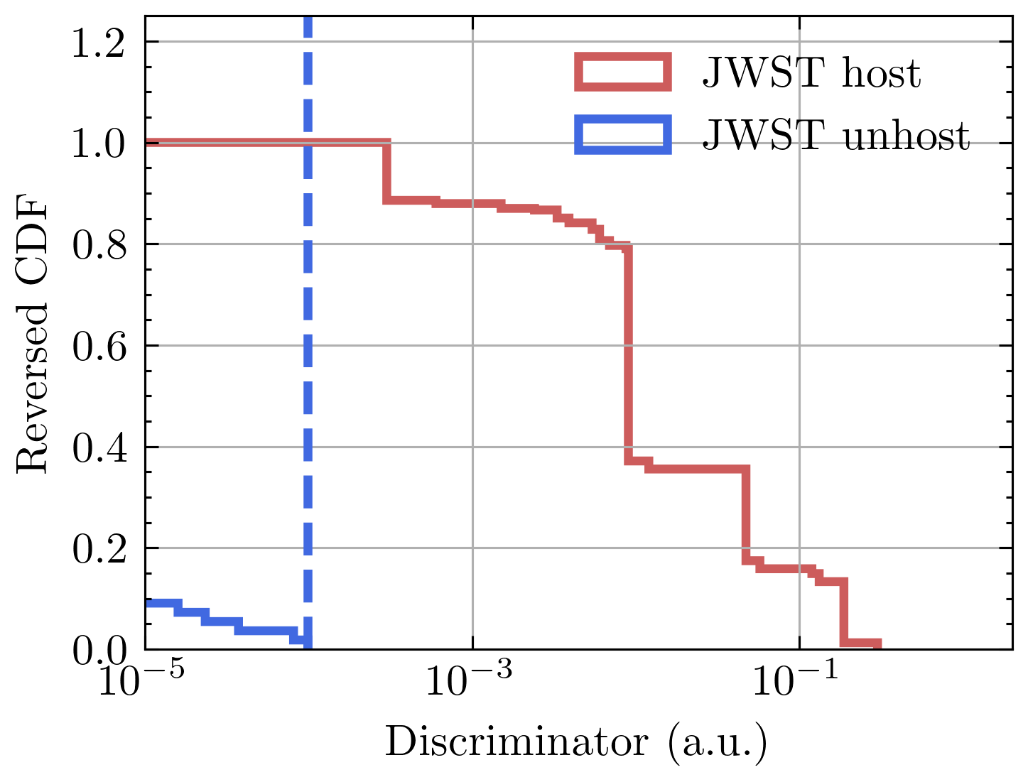
Figure 4: Identification of SLGW Host galaxy. This figure displays the results of host galaxy identification for JWST observations. The $x$-axis represents the discriminator quantity defined in Eq. (10), describing the probability of GGSL time delay w.r.t. SLGW. The $y$-axis represents the reverse cumulative distribution function. The blue curve represents unhosted GGSL systems, while the red curve represents host galaxies with varying magnitudes, SED, and light Sésic profiles. It is worth noting that blue curve includes all the simulated unhosted GGSL systems ($\sim 60$) within an area spanning $20$ square degrees.

Hunting for SLGW and its host galaxy is an important topic in GW astronomy. Its successful discovery is essential for understanding the universe and fundamental physics. However, the long-wave nature of GW forbids us to ‘see’ it directly but only to ‘hear’ it when there is no electromagnetic emission. It results in poor sky localization. Therefore, identifying SLGWs by evaluating the overlapping degrees of GWs’ sky localization region, chirp mass, mass ratio, and other parameters will have a high false positive rate. By using the traditional overlapping method, we have estimated that for $3$G detectors one will pick out $10\sim 15$ lens pair candidates per year together with $50000$ random pairs, which are rejected by the null hypotheses (unlensed hypotheses). To address this challenge, two potential approaches emerge. The first involves a prior knowledge, including parameters such as time delay and magnification ratio [27, 62, 63]. The second avenue involves the use of a more robust technique, commonly known as “joint-parameter estimation” [29, 13], to do a more precise exploration within the SLGWs candidate set.

In this work, we proposed a multi-messenger method triggered by the wave optics effect of the microlensing field embedded in SLGW data. This effect can produce frequency-dependent random fluctuations in the waveform, which can be treated as a smoking gun for SLGW.

In the first step of this method, we analyzed strong lensing events using the template-independent method cWB and the template-dependent method Bilby, respectively. The result in Figure 1 shows that cWB can successfully reconstruct these stochastic microlensing imprints, but Bilby can not. We subsequently generate two datasets: an unlensed dataset and a strong lensing dataset with microlensing. By comparing the matching degree of the cWB and Bilby in the two datasets, we found that the matching of strong lensing events is systematically lower than that of unlensed events due to the microlensing effect, as shown in Figure 2. Therefore, we propose that this mismatching can be treated as a new SLGW identification indicator. Our calculations find that this method can detect roughly $58$ out of $560$ SLGW signals in $3$ years (with $80\%$ duty circle) for $3$G detectors. Importantly, this approach offers the unique advantage of significantly reducing false positives while also requiring minimal computational resources. It achieves this by being less susceptible to coincidental unlensed events pairs (approximately $N^{2}$) and by having a calculation complexity that scales proportionally with $N$. Furthermore, we emphasize that only microlensing fields residing in the lens galaxies can produce these random distortions in the GW waveform of stellar-mass Binary Black Hole (BBH) systems under the framework of general relativity. Thus, identifying a matching outlier using our method strongly suggests the presence of a strong lensing event. In summary, microlensing fringes in SLGWs provide a valuable avenue for SLGW identification, and our method effectively addresses the SLGW identification challenge.

In the second step of this method, we search for the SLGW pairs triggered by the aforementioned identified single-signal events. We identify the multi-signal counterparts by assessing the consistency of sky localization between the multiple signals. This approach, akin to the “overlapping” method, enable us to successfully identify $22$ double-image systems and $3$ quadruple-image systems in $3$ years. Notably, this “overlapping” method offers a lower FAR compared to the traditional “overlapping” method [27]. Its advantage lies in the prerequisite identification of one of the GW signals in the SLGW multi-signal system. This requirement reduces the number of pairs to consider. Here, we employ an “overlapping” sky localization method to identify signal pairs, as it is not susceptible to microlensing bias. Nonetheless, we strongly advocate using a “joint-parameter estimation” approach to improve the confidence in identifying image pairs after mitigating the microlensing bias in SLGWs.

In the last step of this method, we utilize the consistency requirement of time delays between GGSL and SLGW to determine whether the source galaxy in a GGSL system is the host galaxy of the SLGW or not. We find that, with the help of CSST and JWST, we are possible to pin down $1$ quadruple-image strong lensing system within $3$ observation years.

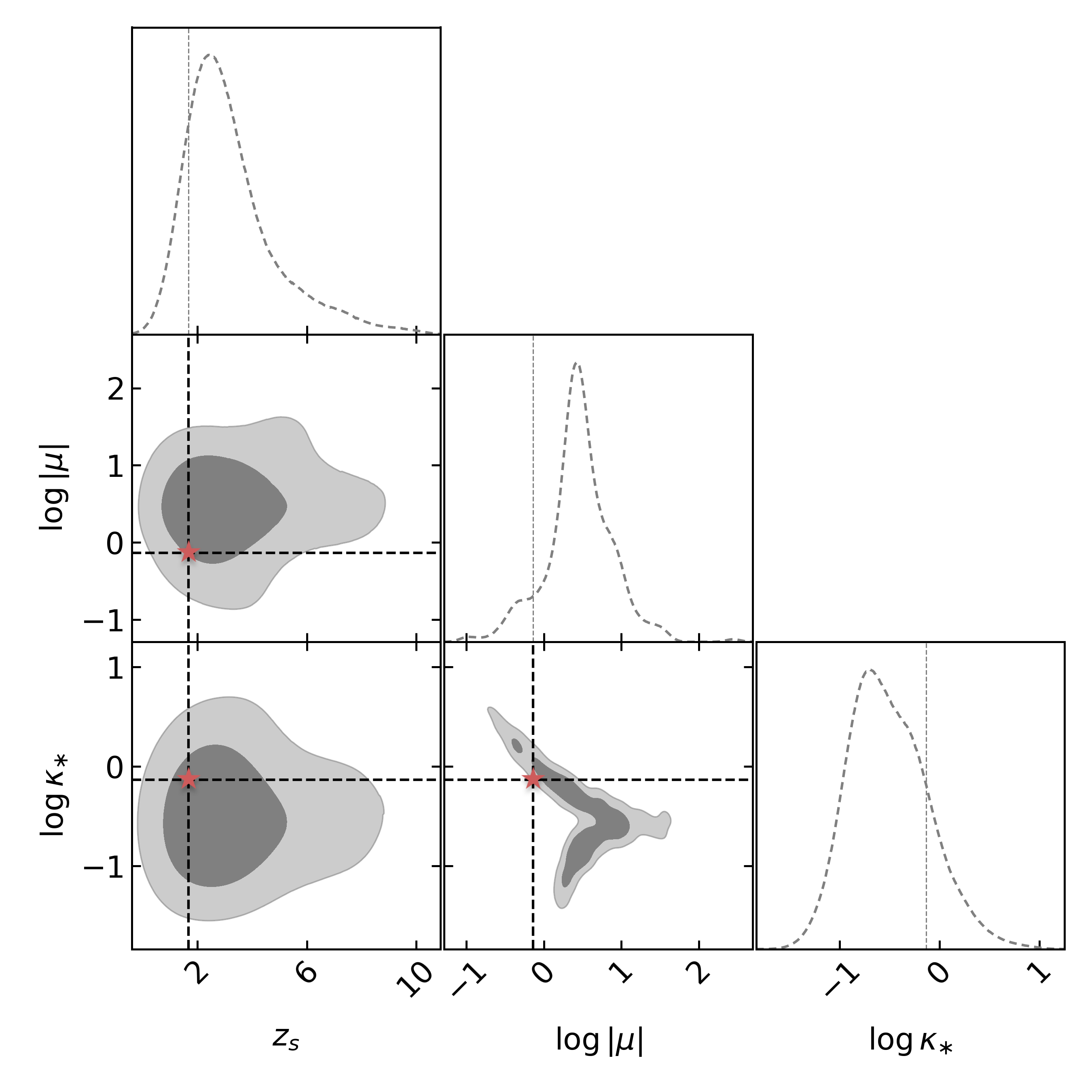
Figure 11: Statistics of the identified event. This figure shows the distribution of source redshift, logarithmic absolute value of magnification, and logarithmic value of $\kappa_{*}$ for all the observed quadruple-image SLGWs over $30$ years observation runs with $80\%$ duty circle. The red star stands for the identified event ID-35 described in the main context.

One might question whether this event is indeed a very special occurrence, to the extent that its discovery was purely accidental. To address this issue, we conduct simulations of SLGWs over $30$ years. The result are shown in Supplementary Figure 11. We can see that the identified quadruple-image system does not have any special characteristics. Therefore, approximately $3$ years of observation time would be enough to identify one SLGW system associated with its host galaxy by using our methodology. Furthermore, it is important to note that the identification of GGSL associated with SLGW could be even more promising. In this analysis, we choose the space-borne telescopes CSST and JWST for the strong lensing image observation. While space-borne telescopes have more accurate angular resolution, their limiting magnitude is lower compared to large ground-based telescopes. This limitation fails to find the fainter events, such as ID-27 and ID-42. To address this challenge, we propose to use large ground-based survey telescopes, such as the Large Synoptic Survey Telescope (LSST) [64, 65], to identify GGSL systems. Subsequently, employing smaller field of view telescopes equipped with adaptive optical systems, like the Thirty Meter Telescope (TMT) [66], to conduct precise follow-up observations. The combined use of these instruments can further enhance our ability to identify all three GGSL systems in our simulation, potentially achieving a detection rate of one system per year.

In summary, we have proposed a multi-messenger, lower FAR, and self-contained methodology for identifying SLGWs and their host galaxies using $3$G GW detectors. This method can significantly facilitate the pursuit of time-delay cosmography and multi-messenger astronomy.

SLGW mock data simulation To validate the method, we follow Refs. [27, 18] to generate a mock data set using the Monte Carlo method. The primary simulation process is as follows.

• We sample the BBH redshift from a theoretical BBH merge rate model in which the merger rate is proportional to the SFR with a delay time $\Delta t=50\mathrm{Myr}$ between the star and BBH formation. The details can be found in Appendix B of Xu et al. [18].

• For the events picked above, we randomly assign BBH masses ($m_{1}$, $m_{2}$), inclination angle ($\iota$), polarization angle ($\psi$), right ascension angle ($\alpha$), declination ($\delta$), merger time ($t_{c}$), and spins ($a_{1}$, $a_{2}$) from the following distributions.

  • $(m_{1},m_{2})\sim\bf\mathrm{power\ law+peak}$ [67].

  • $p(\iota)\propto\sin(\iota)$, $\iota\in[0,\pi]$.

  • $p(\psi)\propto\mathrm{U}(0,\pi)$.

  • $p(\alpha)\propto\mathrm{U}(0,2\pi)$.

  • $p(\delta)\propto\cos(\delta)$, $\delta\in[-\pi/2,\pi/2]$.

  • $p(t_{c})\propto\mathrm{U}(t_{\mathrm{min}},t_{\mathrm{max}})$, where $t_{\mathrm{min}}$ and $t_{\mathrm{max}}$ are the minimum and maximum merger times used in the simulation. Here, we set $t_{\mathrm{max}}-t_{\mathrm{min}}=3\mathrm{yr}\times 80\%$(duty circle).

  • $p(a_{1})\propto\mathrm{U}(0,0.99)$.

  • $p(a_{2})\propto\mathrm{U}(0,0.99)$.

• Calculate the multiple-imaging optical depth $\tau(z_{s})$ for each BBH redshift $z_{s}$ using the SIS optical depth as shown in Haris et al. [27]. Then, generate a random number uniformly distributed between $0$ and $1$ for each BBH event. Compare the calculated optical depth $\tau(z_{s})$ with the generated random number for each event. If the optical depth $\tau(z_{s})$ is greater than the random number, classify it as an SLGW event; otherwise, exclude it from the selection.

• For the selected SLGW samples, we assume a Singular Isothermal Ellipsoid (SIE) lens model [68] and use Lenstronomy [69, 70] to solve the lens equation. The velocity dispersion $\sigma_{v}$ and axis ratio $q$ of SIE are generated from the SDSS galaxy population distribution [71]. Ref. [71] has a typo in axis ratio parameter, we use the corrected form in Ref. [63]. The sample details for these parameters, lens redshift, and source-plane location can be found in Appendix A of Haris et al. [27].

After accounting for the detector’s selection effect in the provided samples, three CE detectors, located at Livingston (USA), Hanford (USA) and Pisa (Italy), can potentially observe approximately $3.5\times 10^{5}$ BBHs and $560$ SLGWs ($256$ strong lensing systems) in $3$ years with $80\%$ duty circle. This result aligns with the findings of Xu et al. [18].

It’s important to note that in this simulation, we assume that an event will be considered as a dectection if it possesses a network matched filter signal-to-noise ratio (SNR) $\geq 12$. Additionally, it’s worth highlighting that, despite using three CE detectors in this simulation, we calculate the SNR starting from a frequency of $20$Hz, not from $1$Hz. Therefore, the result is conservative.

Now, our focus shifts to the simulation of microlensing field. In this study, we utilize the Salpeter initial mass function (IMF) [58] and an elliptical Sésic profile [59] to describe the stellar mass function and density associated with each SLGW. Specifically, we set the stellar mass range to be within $[0.1,1.5]$ solar masses, which aligns with the value employed by Diego et al. [60]. In addition to the stellar mass component, we also consider the presence of remnant objects in the microlensing field. For this purpose, we adopt the initial-final relation (IFR) from Spera et al. [61]. The remnant mass density has been set at $10\%$ of the stellar mass density [55].

Up to this step, we have successfully generated all the essential components for the GW mock data, encompassing both unlensed GWs and SLGWs with microlensing effects.

SLGW finder and pairing We search for SLGW multi-signal pairs based on the parameter overlapping degree between two GW events. To do this, we utilize the “overlapping” method introduced in Haris et al. [27].

$$\mathcal{B}_{\mathrm{U}}^{\mathrm{L}}:=\int d\bm{\theta}\frac{P\left(\bm{\theta}\mid d_{1}\right)P\left(\bm{\theta}\mid d_{2}\right)}{P(\bm{\theta})}\\ ,$$ (6)

where $\theta$ represents the GW parameter, $d_{1}$ and $d_{2}$ denote the strain data for event $1$ and event $2$, respectively. $P(\bm{\theta})$ corresponds to the prior distribution, and $P\left(\bm{\theta}\mid d_{1}(d_{2})\right)$ represents the posterior distribution.

In this calculation, we only consider two parameters, ra (right ascension) and dec (declination). This choice is motivated by the fact that the presence of the microlensing effect can introduce significant bias in intrinsic GW parameters such as mass ratio $q$ and chirp mass $\mathcal{M}$. Including these parameters in the Bayesian factor calculation could diminish the authentication capability.

To quantify the bias introduced by the microlensing effect, we define the “BIAS” level using the following equation

$$\mathrm{BIAS}=\frac{|\bar{x}_{\text{micro }}-x_{\text{inject }}|}{\sqrt{\sigma^{2}\left(x_{\text{micro }}\right)}}\\ ,$$ (7)

where $\bar{x}_{\text{micro}}$ and $\sqrt{\sigma^{2}\left(x_{\text{micro }}\right)}$ represent the mean value and standard deviation of the parameter posterior distribution for SLGW with microlensing effect, respectively. $x_{\text{inject}}$ is the injected true value. $x$ represents the GW parameters listed in the figure.

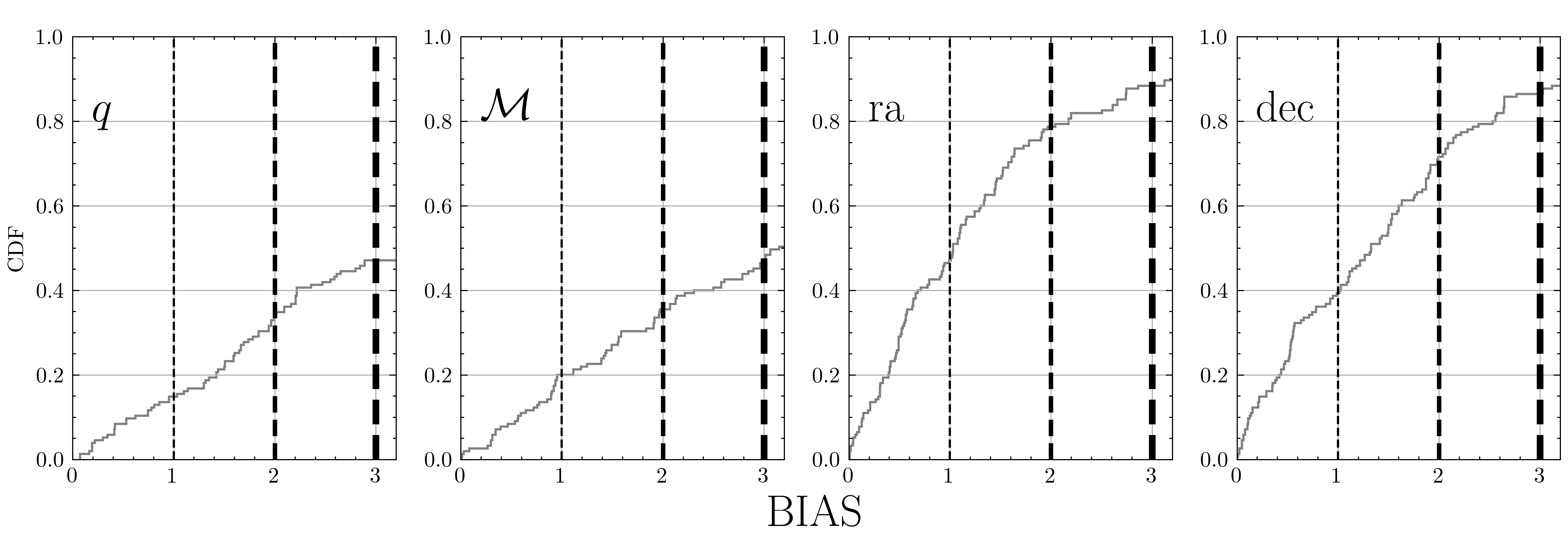
Figure 6: SLGW parameter bias. This figure shows the parameter bias for intrinsic parameters: mass ratio $q$ and chirp mass $\mathcal{M}$, and extrinsic parameters: right ascension ra, and declination dec. The $y$-axis is the cumulative probability distribution function of the quantity defined in Eq. (7). The $x$-axis denotes the BIAS value. Three dashed vertical curves with different line widths correspond to $1~{}\sigma$, $2~{}\sigma$ and $3~{}\sigma$ bias level.

In Figure 6, we illustrate the parameter bias for all the selected single-signal SLGW events from Figure 2 and their multi-signal counterparts. The $y$-axis represents the cumulative probability distribution function of the quantity defined in Eq. (7). The $x$-axis denotes the bias level. Three dashed vertical curves with different line widths correspond to $1~{}\sigma$, $2~{}\sigma$ and $3~{}\sigma$ bias level. The first and second columns of the figure display the results for intrinsic parameters, including $q$, $\mathcal{M}$. The third and fourth columns show the results for extrinsic parameters, including RA and DEC. One can see that for $q$ and $\mathcal{M}$, there are more than $50\%$ events out side of $3\sigma$ interval. However, for ra and dec, these values is only about $10\%$. Hence, we can conclude that the microlensing induced bias is more serious for the intrinsic parameters than the extrinsic parameters.

To demonstrate the identification efficiency of this method, it is essential to evaluate the FAR of this method. The FAR per pair is defined as

$$\mathrm{FAR}_{\rm per~{}pair}=\frac{N_{\mathrm{unlens}}(\mathcal{B_{\mathrm{U}}}>\mathcal{B}_{\mathrm{L}})}{N_{\mathrm{unlens}}(\mathrm{total})}\\ ,$$ (8)

where $N_{\mathrm{unlens}}$ is the number of randomly matched unlensed pairs, and $\mathcal{B}_{\mathrm{L}}$ is the Bayes factor of SLGW multi-signal pair. The FAR per year is defined as

$$\mathrm{FAR}_{\rm per~{}year}=\mathrm{FAR}_{\rm per~{}pair}\times N_{\mathrm{lens-unlens}}\\ ,$$ (9)

where $N_{\mathrm{lens-unlens}}$ is the pair number between identified single-signal SLGWs and unlensed GWs in the sky localization of SLGWs.

It is worth noting that $N_{\mathrm{lens-unlens}}$ is proportional to the number of unlensed GWs ($\mathcal{O}(N)$) but not proportional to the number of randomly matched unlensed pairs ($\mathcal{O}(N^{2})$). Consequently, the $\mathrm{FAR}_{\mathrm{per~{}year}}$ calculated using this method is significantly lower than that obtained by directly using the “overlapping” method to find the SLGW image pairs without prior knowledge about the microlensing.

GGSL simulation and host galaxy identification In this section, we introduce our host galaxy identification method for SLGWs. We first generate a mock dataset for GGSL by utilizing a JWST mock catalog known as JAGUAR [72]. For the unhosted GGSL systems, we employ the optical depth method, which is identical to the one used for generating SLGWs, to simulate GGSL events across a $20$ square degrees region. We find that there are roughly $3300$ GGSL systems with Einstein radius $\theta_{E}>0.2^{\prime\prime}$ in $1$ square degree. This number is consistent with the simulation result of the CSST strong lensing group (private communication). Subsequently, we randomly select lens galaxy magnitudes and light Sésic radius using the fundamental plane [73]. There is a typographical error in Goldsteinet al.[73], so we utilize the corrected formula provided in Wempe et al. [74]. For the host galaxy, we collect the galaxy properties, such as SED and light Sésic profile, via a thin shell $[z_{s}-\Delta z_{s},z_{s}+\Delta z_{s}]$, where $z_{s}$ is the real host galaxy redshift and the shell width is chosen as $\Delta z_{s}=0.01$. The true host galaxy property parameter is assigned according to the above samples. We then rank the host probability based on the SFR of each samples over the past $50~{}\mathrm{Myr}$.

In order to find the host galaxies, we propose a targeted observation strategy. First, we conduct an ordinary survey ($600s$ exposure time) utilizing the CSST [75], which has a field of view around $1.1$ square degrees. The primary objective of this survey is to systematically scan the sky localization envelope of multi-signal SLGWs and subsequently select the GGSL systems which are observable. Here, we employ two criteria to assess the observability of GGSL systems: $M_{\mathrm{AB}}<26$, and $\theta_{\mathrm{E}}^{2}>r_{s}^{2}+(s/2)^{2}$, where $\theta_{\mathrm{E}}$ represents the Einstein radius, $s$ denotes the seeing (for CSST $s=0.135^{{}^{\prime\prime}}$), and $r_{s}$ stands for the unlensed source size. The second criteria denotes the requirement of being able to distinguish multiple images of each GGSL. It is worth noting that we scan the sky localization envelope region, rather than the overlapping region, of the multiple GW counterparts. In Supplementary Figure 7, we show the sky localization result for the three SLGWs identified in Figure 3. Each panel has four counters representing quadruple counterparts. It is obviously that the injected sky location (dashed curve) is safely within the envelope of the sky localization.

Subsequently, we propose using the JWST [76], which has a higher limiting magnitude, for follow-up observations ($1000s$) for each of the targeted GGSLs. This strategy is cost-effective since CSST observation will only select around $3$ quadurple-image GGSLs per square degree. Hence, the subsequent JWST observations time is about $1$ hour in total for $3$ candidates.

In Supplementary Figure 8, we depict the probability distribution of host galaxy apparent magnitudes for the three identified SLGWs. The host galaxy number density is weighted by the SFR according to the BBH population model. In this figure, red histogram represents the CSST result, and blue histogram represents the JWST one. The apparent magnitude differences between these two telescopes result from the filter band. Specifically, we adopt the Sloan $r$ band for CSST and the F$200$W band for JWST. It is worth noting that our current analysis assumes only single photometry band, and the multi-band analysis will definitely improve the current results. The grey shaded region indicates events that cannot be observed by CSST due to its limited magnitude (assuming CSST limiting magnitude of $\mathrm{M}_{AB}=26$). From this figure, it is clear that for event ID-35, there is a remarkably high probability (approximately $80\%$) of observing its host galaxy. Hence, we will focus our analysis primarily on this event.

To identify host galaxies, we ask for the consistency of time delays between GGSL and SLGW measurements. In this paper, we use the relative time delay difference as the discriminator. For quadruple-image systems, the discriminator consists of two independent components: $\Delta t_{1,2}/\Delta t_{1,3}$ and $\Delta t_{1,2}/\Delta t_{1,4}$. Here, $\Delta t_{1,2}$ represents the time delay difference between image $1$ and $2$ (with $\Delta t_{1,3}$ and $\Delta t_{1,4}$ having similar meanings). In detail, the discriminator is defined as

$$P_{\mathrm{dis}}=P_{\mathrm{GGSL}}(\frac{\Delta t_{1,2}}{\Delta t_{1,3}})|_{\mathrm{SLGW}}\times P_{\mathrm{GGSL}}(\frac{\Delta t_{1,2}}{\Delta t_{1,4}})|_{\mathrm{SLGW}}\\ ,$$ (10)

where $P_{\mathrm{GGSL}}(x)|_{\mathrm{SLGW}}$ represents the probability density of time delays derived from GGSL results at the specific measurement point of SLGW. It is evident that the greater the consistency between GGSL and SLGW, the larger this quantity becomes. The advantage of employing relative time delays as the discriminator is their independence from cosmological parameters, such as the Hubble constant. Up to this point, we have introduced all the simulation procedures and methods. To provide a clearer representation, we illustrate the main steps of our methodology in Figure 5.

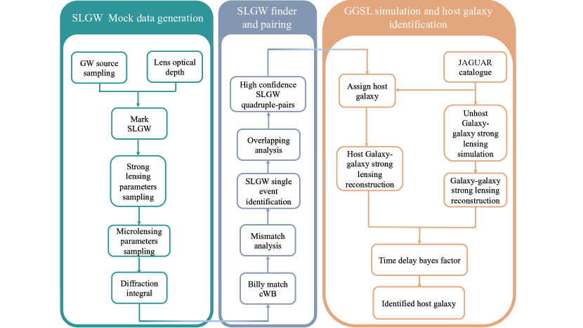
Figure 5: Flowchart of the full simulation. This figure shows the simulation procedures introduced in Method section. Difference colors stand for three main simulation sections.

Data availability The code that support the findings of this study are available from the corresponding author upon request.

Supplementary

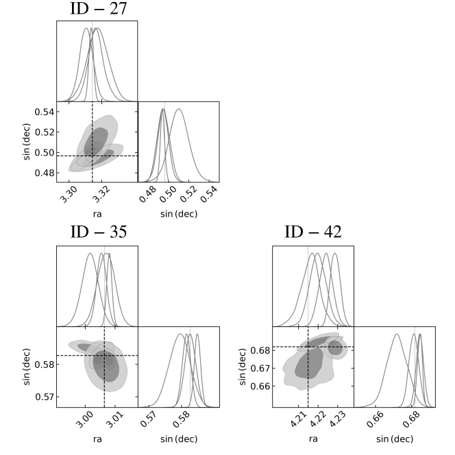
Figure 7: Sky localization of three identified quadruple-image SLGWs. This figure displays the sky localization of the three high-confidence quadruple-image SLGWs. The titles in three corner figures stand for event indices in Figure 3

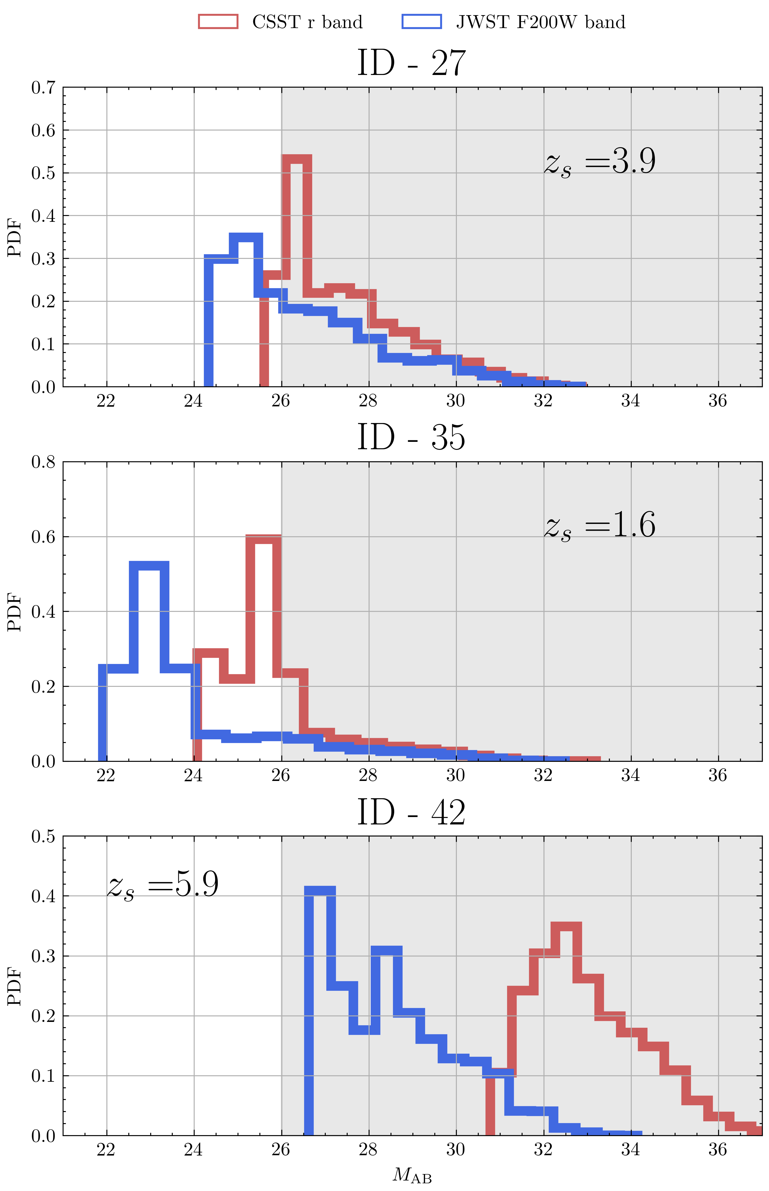
Figure 8: Probability distribution function of host galaxy magnitude. This figure presents the host galaxy magnitude distribution for the three quadruple-image SLGWs identified in Figure 3. The red and blue curves represent the result for CSST and JWST, respectively. The grey shaded region stand for the magnitude greater than $26$ where the host galaxy cannot be observed by using the CSST main survey.

Acknowledgements This work is supported in part by the National Key R&D Program of China No. 2021YFC2203001, No. 2020YFC2201502 and No. 2021YFA0718304, and supported in part by the National Natural Science Foundation of China Grants No. 11821505, No.11991052 and No.12235019.

Author contributions All authors provided ideas throughout the project and comments on the manuscript. XS contributed in calculating and writing the draft. XC contributed in generating the microlensing fields. BH contributed in proposing the idea and writing the draft. RGC contributed in proposing the idea and writing the draft.

Competing interests The authors have no competing interests.

References

- [1] Abbott, B. et al. GWTC-1: A Gravitational-Wave Transient Catalog of Compact Binary Mergers Observed by LIGO and Virgo during the First and Second Observing Runs. Phys. Rev. X 9, 031040 (2019). 1811.12907.
- [2] Abbott, R. et al. GWTC-2: Compact Binary Coalescences Observed by LIGO and Virgo During the First Half of the Third Observing Run. Phys. Rev. X 11, 021053 (2021). 2010.14527.
- [3] Abbott, R. et al. GWTC-3: Compact Binary Coalescences Observed by LIGO and Virgo During the Second Part of the Third Observing Run. arXiv e-prints arXiv:2111.03606 (2021). 2111.03606.
- [4] Aasi, J. et al. Advanced ligo. Classical and Quantum Gravity 32, 074001 (2015). URL http://dx.doi.org/10.1088/0264-9381/32/7/074001.
- [5] Acernese, F. et al. Advanced virgo: a second-generation interferometric gravitational wave detector. Classical and Quantum Gravity 32, 024001 (2014). URL http://dx.doi.org/10.1088/0264-9381/32/2/024001.
- [6] Akutsu, T. et al. KAGRA: 2.5 Generation Interferometric Gravitational Wave Detector. Nature Astron. 3, 35–40 (2019). 1811.08079.
- [7] Unnikrishnan, C. S. IndIGO and LIGO-India: Scope and plans for gravitational wave research and precision metrology in India. Int. J. Mod. Phys. D 22, 1341010 (2013). 1510.06059.
- [8] Li, S.-S., Mao, S., Zhao, Y. & Lu, Y. Gravitational lensing of gravitational waves: A statistical perspective. Mon. Not. Roy. Astron. Soc. 476, 2220–2229 (2018). 1802.05089.
- [9] Oguri, M. Effect of gravitational lensing on the distribution of gravitational waves from distant binary black hole mergers. Mon. Not. Roy. Astron. Soc. 480, 3842–3855 (2018). 1807.02584.
- [10] Hannuksela, O. A. et al. Search for gravitational lensing signatures in LIGO-Virgo binary black hole events. Astrophys. J. Lett. 874, L2 (2019). 1901.02674.
- [11] Kim, K., Lee, J., Yuen, R. S. H., Hannuksela, O. A. & Li, T. G. F. Identification of Lensed Gravitational Waves with Deep Learning. Astrophys. J. 915, 119 (2021). 2010.12093.
- [12] McIsaac, C. et al. Search for strongly lensed counterpart images of binary black hole mergers in the first two LIGO observing runs. Phys. Rev. D 102, 084031 (2020). 1912.05389.
- [13] Liu, X., Magana Hernandez, I. & Creighton, J. Identifying strong gravitational-wave lensing during the second observing run of Advanced LIGO and Advanced Virgo. Astrophys. J. 908, 97 (2021). 2009.06539.
- [14] Abbott, R. et al. Search for Lensing Signatures in the Gravitational-Wave Observations from the First Half of LIGO–Virgo’s Third Observing Run. Astrophys. J. 923, 14 (2021). 2105.06384.
- [15] Abbott, R. et al. Search for gravitational-lensing signatures in the full third observing run of the LIGO-Virgo network (2023). 2304.08393.
- [16] Punturo, M., Lück, H. & Beker, M. A Third Generation Gravitational Wave Observatory: The Einstein Telescope, vol. 404 of Astrophysics and Space Science Library, 333 (2014).
- [17] Abbott, B. P. et al. Exploring the Sensitivity of Next Generation Gravitational Wave Detectors. Class. Quant. Grav. 34, 044001 (2017). 1607.08697.
- [18] Xu, F., Ezquiaga, J. M. & Holz, D. E. Please Repeat: Strong Lensing of Gravitational Waves as a Probe of Compact Binary and Galaxy Populations. Astrophys. J. 929, 9 (2022). 2105.14390.
- [19] Sereno, M., Jetzer, P., Sesana, A. & Volonteri, M. Cosmography with strong lensing of LISA gravitational wave sources. Mon. Not. Roy. Astron. Soc. 415, 2773 (2011). 1104.1977.
- [20] Liao, K., Fan, X.-L., Ding, X.-H., Biesiada, M. & Zhu, Z.-H. Precision cosmology from future lensed gravitational wave and electromagnetic signals. Nature Commun. 8, 1148 (2017). [Erratum: Nature Commun. 8, 2136 (2017)], 1703.04151.
- [21] Hannuksela, O. A., Collett, T. E., Çalışkan, M. & Li, T. G. F. Localizing merging black holes with sub-arcsecond precision using gravitational-wave lensing. Mon. Not. Roy. Astron. Soc. 498, 3395–3402 (2020). 2004.13811.
- [22] Yu, H., Zhang, P. & Wang, F.-Y. Strong lensing as a giant telescope to localize the host galaxy of gravitational wave event. Mon. Not. Roy. Astron. Soc. 497, 204–209 (2020). 2007.00828.
- [23] Baker, T. & Trodden, M. Multimessenger time delays from lensed gravitational waves. Phys. Rev. D 95, 063512 (2017). 1612.02004.
- [24] Collett, T. E. & Bacon, D. Testing the speed of gravitational waves over cosmological distances with strong gravitational lensing. Phys. Rev. Lett. 118, 091101 (2017). 1602.05882.
- [25] Fan, X.-L., Liao, K., Biesiada, M., Piorkowska-Kurpas, A. & Zhu, Z.-H. Speed of Gravitational Waves from Strongly Lensed Gravitational Waves and Electromagnetic Signals. Phys. Rev. Lett. 118, 091102 (2017). 1612.04095.
- [26] Nakamura, T. T. Gravitational lensing of gravitational waves from inspiraling binaries by a point mass lens. Phys. Rev. Lett. 80, 1138–1141 (1998).
- [27] Haris, K., Mehta, A. K., Kumar, S., Venumadhav, T. & Ajith, P. Identifying strongly lensed gravitational wave signals from binary black hole mergers (2018). 1807.07062.
- [28] Goyal, S., D., H., Kapadia, S. J. & Ajith, P. Rapid identification of strongly lensed gravitational-wave events with machine learning. Phys. Rev. D 104, 124057 (2021). 2106.12466.
- [29] Lo, R. K. L. & Magaña Hernandez, I. A Bayesian statistical framework for identifying strongly-lensed gravitational-wave signals (2021). 2104.09339.
- [30] Janquart, J., Hannuksela, O. A., K., H. & Van Den Broeck, C. A fast and precise methodology to search for and analyse strongly lensed gravitational-wave events. Mon. Not. Roy. Astron. Soc. 506, 5430–5438 (2021). 2105.04536.
- [31] Dai, L. & Venumadhav, T. On the waveforms of gravitationally lensed gravitational waves (2017). 1702.04724.
- [32] Wang, Y., Lo, R. K. L., Li, A. K. Y. & Chen, Y. Identifying Type II Strongly Lensed Gravitational-Wave Images in Third-Generation Gravitational-Wave Detectors. Phys. Rev. D 103, 104055 (2021). 2101.08264.
- [33] Vitale, S. & Evans, M. Parameter estimation for binary black holes with networks of third-generation gravitational-wave detectors. prd 95, 064052 (2017). 1610.06917.
- [34] Çalışkan, M., Ezquiaga, J. M., Hannuksela, O. A. & Holz, D. E. Lensing or luck? False alarm probabilities for gravitational lensing of gravitational waves (2022). 2201.04619.
- [35] Diego, J. M., Broadhurst, T. & Smoot, G. Evidence for lensing of gravitational waves from LIGO-Virgo data. Phys. Rev. D 104, 103529 (2021). 2106.06545.
- [36] Millon, M. et al. COSMOGRAIL XIX: Time delays in 18 strongly lensed quasars from 15 years of optical monitoring. Astron. Astrophys. 640, A105 (2020). 2002.05736.
- [37] Millon, M. et al. TDCOSMO - II. Six new time delays in lensed quasars from high-cadence monitoring at the MPIA 2.2 m telescope. Astron. Astrophys. 642, A193 (2020). 2006.10066.
- [38] Choi, Y.-Y., Park, C. & Vogeley, M. S. Internal and Collective Properties of Galaxies in the Sloan Digital Sky Survey. Astrophys. J. 658, 884–897 (2007). astro-ph/0611607.
- [39] Tinker, J. L. et al. Toward a halo mass function for precision cosmology: The Limits of universality. Astrophys. J. 688, 709–728 (2008). 0803.2706.
- [40] Ali, S., Stoikos, E., Meade, E., Kesden, M. & King, L. Detectability of strongly lensed gravitational waves using model-independent image parameters. Phys. Rev. D 107, 103023 (2023). 2210.01873.
- [41] Klimenko, S. et al. cwb pipeline library: 6.4.0 (2021). URL https://doi.org/10.5281/zenodo.4419902.
- [42] Klimenko, S. et al. Method for detection and reconstruction of gravitational wave transients with networks of advanced detectors. Phys. Rev. D 93, 042004 (2016). 1511.05999.
- [43] Relton, P. et al. Addressing the challenges of detecting time-overlapping compact binary coalescences. Phys. Rev. D 106, 104045 (2022). 2208.00261.
- [44] Hannam, M. et al. Simple Model of Complete Precessing Black-Hole-Binary Gravitational Waveforms. Phys. Rev. Lett. 113, 151101 (2014). 1308.3271.
- [45] LIGO Scientific Collaboration. LALSuite: LIGO Scientific Collaboration Algorithm Library Suite. Astrophysics Source Code Library, record ascl:2012.021 (2020). 2012.021.
- [46] Nitz, A. et al. gwastro/pycbc: v2.0.2 release of pycbc (2022). URL https://doi.org/10.5281/zenodo.6324278.
- [47] Dobler, G. & Keeton, C. R. Microlensing of Lensed Supernovae. Astrophys. J. 653, 1391–1399 (2006). astro-ph/0608391.
- [48] Chen, X., Shu, Y., Li, G. & Zheng, W. FRBs Lensed by Point Masses. II. The Multipeaked FRBs from the Point View of Microlensing. Astrophys. J. 923, 117 (2021). 2110.07643.
- [49] Zheng, W., Chen, X., Li, G. & Chen, H.-z. An Improved GPU-based Ray-shooting Code for Gravitational Microlensing. Astrophys. J. 931, 114 (2022). 2204.10871.
- [50] Shan, X., Li, G., Chen, X., Zheng, W. & Zhao, W. Wave effect of gravitational waves intersected with a microlens field: a new algorithm and supplementary study (2022). 2208.13566.
- [51] Schneider, P., Ehlers, J. & Falco, E. E. Gravitational Lenses (Springer New York, NY, 1992).
- [52] Wambsganss, J. Ph.D. thesis, - (1990).
- [53] Diego, J. M. et al. Observational signatures of microlensing in gravitational waves at LIGO/Virgo frequencies. Astron. Astrophys. 627, A130 (2019). 1903.04513.
- [54] Mishra, A., Meena, A. K., More, A., Bose, S. & Bagla, J. S. Gravitational lensing of gravitational waves: effect of microlens population in lensing galaxies. Mon. Not. Roy. Astron. Soc. 508, 4869–4886 (2021). 2102.03946.
- [55] Meena, A. K., Mishra, A., More, A., Bose, S. & Bagla, J. S. Gravitational lensing of gravitational waves: Probability of microlensing in galaxy-scale lens population. Mon. Not. Roy. Astron. Soc. 517, 872–884 (2022). 2205.05409.
- [56] Ashton, G. et al. BILBY: A user-friendly Bayesian inference library for gravitational-wave astronomy. Astrophys. J. Suppl. 241, 27 (2019). 1811.02042.
- [57] Kim, K. & Liu, A. Can we discern microlensed gravitational-wave signals from the signal of precessing compact binary mergers? (2023). 2301.07253.
- [58] Salpeter, E. E. The Luminosity Function and Stellar Evolution. ApJ 121, 161 (1955).
- [59] Vernardos, G. Microlensing flux ratio predictions for euclid. Monthly Notices of the Royal Astronomical Society 483, 5583–5594 (2018). URL https://doi.org/10.1093%2Fmnras%2Fsty3486.
- [60] Diego, J. M. et al. Microlensing and the type Ia supernova iPTF16geu. Astron. Astrophys. 662, A34 (2022). 2112.04524.
- [61] Spera, M., Mapelli, M. & Bressan, A. The mass spectrum of compact remnants from the PARSEC stellar evolution tracks. MNRAS 451, 4086–4103 (2015). 1505.05201.
- [62] More, A. & More, S. Improved statistic to identify strongly lensed gravitational wave events. Mon. Not. Roy. Astron. Soc. 515, 1044–1051 (2022). 2111.03091.
- [63] Wierda, A. R. A. C., Wempe, E., Hannuksela, O. A., Koopmans, L. e. V. E. & Van Den Broeck, C. Beyond the Detector Horizon: Forecasting Gravitational-Wave Strong Lensing. Astrophys. J. 921, 154 (2021). 2106.06303.
- [64] Abell, P. A. et al. LSST Science Book, Version 2.0 (2009). 0912.0201.
- [65] Smith, G. P., Robertson, A., Bianconi, M. & Jauzac, M. Discovery of Strongly-lensed Gravitational Waves - Implications for the LSST Observing Strategy (2019). 1902.05140.
- [66] Skidmore, W. et al. Thirty Meter Telescope Detailed Science Case: 2015. Res. Astron. Astrophys. 15, 1945–2140 (2015). 1505.01195.
- [67] Abbott, B. P. et al. Binary Black Hole Population Properties Inferred from the First and Second Observing Runs of Advanced LIGO and Advanced Virgo. Astrophys. J. Lett. 882, L24 (2019). 1811.12940.
- [68] Kormann, R., Schneider, P. & Bartelmann, M. Isothermal elliptical gravitational lens models. A&A 284, 285–299 (1994).
- [69] Birrer, S. & Amara, A. lenstronomy: Multi-purpose gravitational lens modelling software package. Physics of the Dark Universe 22, 189–201 (2018). 1803.09746.
- [70] Birrer, S. et al. lenstronomy II: A gravitational lensing software ecosystem. The Journal of Open Source Software 6, 3283 (2021). 2106.05976.
- [71] Collett, T. E. The Population of Galaxy-Galaxy Strong Lenses in Forthcoming Optical Imaging Surveys. ApJ 811, 20 (2015). 1507.02657.
- [72] Williams, C. C. et al. The JWST Extragalactic Mock Catalog: Modeling Galaxy Populations from the UV through the Near-IR over 13 Billion Years of Cosmic History. ApJS 236, 33 (2018). 1802.05272.
- [73] Goldstein, D. A., Nugent, P. E. & Goobar, A. Rates and Properties of Supernovae Strongly Gravitationally Lensed by Elliptical Galaxies in Time-domain Imaging Surveys. Astrophys. J. Suppl. 243, 6 (2019). 1809.10147.
- [74] Wempe, E., Koopmans, L. V. E., Wierda, A. R. A. C., Hannuksela, O. A. & Broeck, C. v. d. A lensing multi-messenger channel: Combining LIGO-Virgo-Kagra lensed gravitational-wave measurements with Euclid observations (2022). 2204.08732.
- [75] Zhan, H. Consideration for a large-scale multi-color imaging and slitless spectroscopy survey on the Chinese space station and its application in dark energy research. Scientia Sinica Physica, Mechanica & Astronomica 41, 1441 (2011).
- [76] Gardner, J. P. et al. The James Webb Space Telescope. Space Sci. Rev. 123, 485 (2006). astro-ph/0606175.