lenstronomy: multi-purpose gravitational lens modelling software package

Abstract

We present lenstronomy, a multi-purpose open-source gravitational lens modeling python package. lenstronomy is able to reconstruct the lens mass and surface brightness distributions of strong lensing systems using forward modelling. lenstronomy supports a wide range of analytic lens and light models in arbitrary combination. The software is also able to reconstruct complex extended sources (Birrer et. al 2015) as well as being able to model point sources. We designed lenstronomy to be stable, flexible and numerically accurate, with a clear user interface that could be deployed across different platforms. Throughout its development, we have actively used lenstronomy to make several measurements including deriving constraints on dark matter properties in strong lenses, measuring the expansion history of the universe with time-delay cosmography, measuring cosmic shear with Einstein rings and decomposing quasar and host galaxy light. The software is distributed under the MIT license. The documentation, starter guide, example notebooks, source code and installation guidelines can be found at https://lenstronomy.readthedocs.io.

1 Introduction

Strong gravitational lensing, the bending of light by foreground masses to such an extent that multiple images of the same source are formed, is an important phenomenon that can be used to probe the matter distribution and geometry of the universe. The detailed reconstruction of the light paths can be used to test the nature of the unknown components dark matter and dark energy. These dominate the matter-energy content of the Universe today.

In strong lensing studies, significant progress has been made in recent years in both quantifying the small scale matter distribution, with techniques such as gravitational imaging Vegetti et al. (2010, 2012); Hezaveh et al. (2016); Birrer et al. (2017a); Vegetti et al. (2018) and flux ratio anomalies Mao and Schneider (1998); Metcalf and Madau (2001); Dalal and Kochanek (2002); Nierenberg et al. (2014); Xu et al. (2015); Nierenberg et al. (2017), and measuring the expansion history of the universe, with time-delay cosmography Refsdal (1964); Schechter et al. (1997); Treu and Koopmans (2002); Suyu et al. (2010, 2014); Birrer et al. (2016); Bonvin et al. (2017). These successes have in part been made possible due to the development of state-of-the-art lens modelling software and algorithms that can extract the required lensing information from high resolution imaging data. Several of the codes used for doing this have been made publicly available to the community (see A).

From the current and upcoming surveys, the sample of known strong lenses is rapidly increasing (see e.g. Agnello et al., 2015; Nord et al., 2016; Schechter et al., 2017; Lin et al., 2017; Jacobs et al., 2017; Ostrovski et al., 2017; Williams et al., 2018; Lemon et al., 2018) and Treu et al. (submitted). This enlarged sample enables competitive measurements of the Hubble constant (see e.g. Treu and Marshall, 2016; Shajib et al., 2018; Suyu et al., 2018) as well as can strengthen constraints on dark matter properties on sub-galactic scales (see e.g. forecast by Gilman et al., 2018). To fully exploit the science potential of these new strong lensing data, our modelling tools need to be continually developed and improved.

In this publication, we present the first public release of lenstronomy, which is an open source multi-purpose strong lens modelling software package. lenstronomy has been used as a research tool throughout its development. This includes being used for time-delay cosmography (Birrer et al., 2016, 2018b), lensing substructure analysis (Birrer et al., 2017a), line-of-sight shear measurements from an Einstein ring (Birrer et al., 2017b) and its forecast to measure cosmic shear with Einstein rings (Birrer et al., 2018a). Each of these tasks required the modelling of Hubble Space Telescope (HST) imaging data at the pixel level.

We developed lenstronomy to be stable, flexible and numerically accurate, with a clear Application programming interface (API) that could be used across different platforms. The lenstronomy software architecture was designed to be able to scale from the current era, where individual lenses are studied in detail, to the case where several hundreds of lenses, from future surveys, will need to be processed.

Given that an essential part of precision cosmology is the control of systematic errors, it is important for the community to develop multiple independent pipelines. This allows for the cross-checks that are necessary for complex precision measurements. Community standard benchmark efforts also make important contributions. For instance, the time-delay lens modelling challenge (Ding et al., 2018) offers a realistic and blind comparison framework in the domain of cosmography. Similar efforts are underway by the substructure lensing community. The public release of lenstronomy enables a transparent and effective comparison with other software used in strong lensing.

lenstronomy includes, but is not limited to, the methods presented in (Birrer et al., 2015). This includes a linear source reconstruction method based on Shapelet (Refregier, 2003) basis sets, a Particle Swarm Optimization (Kennedy and Eberhart, 1995) for optimizing the non-linear lens model parameters and a MCMC framework for Bayesian parameter inference (emcee Foreman-Mackey et al., 2013). The software supports a high dynamic range in angular scales, complexity in source and lens models, can handle various image qualities and meets the requirements for diverse science applications. Furthermore, lenstronomy enables a consistent integration of imaging, time-delay and kinematic data to provide model constraints.

There is continued development and support of lenstronomy to expand its scope and scientific application for a growing user community.

This paper is structured as follows: In Section 2, we provide an overview of the software architecture and deployment, including installation and dependencies. In Section 3, we describe the core modules of lenstronomy with some simple examples of how to use them. We provide some modelling examples in Section 4 to demonstrate the capabilities and flexibility of lenstronomy. In Section 5, we give some science application highlights. We summarize in Section 6.

This publication is accompanied by a public release of the source code with extensive online documentation. Additionally, we provide Jupyter notebook examples for different science cases. We refer the reader to these online resources for the most updated version of the software package.

2 Package overview

lenstronomy is an open source software package developed in python (Rossum, 1995). Distribution is granted through the MIT open source software license. lenstronomy relies on packages included in the python standard library and the proven open-source libraries numpy , scipy , astropy (Astropy Collaboration et al., 2013), and matplotlib (Hunter, 2007). For optimization and parameter inference routines, CosmoHammer (Akeret et al., 2013) is used, which supports Message Passing Interface (MPI) and allows for massive parallelization of the emcee (Foreman-Mackey et al., 2013) algorithm.

The stable release version can be installed at the command line via pip:

⬇ $ pip install lenstronomy --user

lenstronomy is compatible with both python2 and python3. The code design and development follow effective practices for scientific computing. The development is coordinated on GitHub and stable versions are released through PyPi - the python packaging index. This full integration of lenstronomy in the python packaging environment allows third party to release and share software packages, analysis routines and work-flows that rely upon lenstronomy.

Extensive tests have been added to lenstronomy  which allows us to develop the package using a Continuous Integration (CI) process. The tests are performed on a virtual environment to ensure cross-platform stability and the test coverage report is publicly available. Documentation for the various routines and classes are provided through sphinx and are available on ReadtheDocs. To make use of lenstronomy, a start guide and several application examples are provided in the form of Jupyter notebooks in an extension module.

lenstronomy is structured in multiple independent modules, each consisting of multiple classes and sub-packages. These modules execute specific tasks and come with well-defined API. Among the core modules are:

1. LensModel: Provides the lensing functionalities. The full functionality is supported with an arbitrary superposition of individual lens models (Section 3.1).

2. LightModel: Enables a variety of surface brightness descriptions and profiles. See Section 3.2.

3. PointSource: Handles the point sources (Section 3.3).

4. Data: Handling all data specific tasks. Including Point-Spread function (PSF), coordinate systems and noise properties (Section 3.4).

5. ImSim: Simulates images. Queries the specifications made in LensModel, LightModel, PointSource and Data (Section 3.5).

6. Sampling: Performs the sampling of the parameter space. Aside from the Sampling class that offers pre-defined sampling algorithm, the module includes the , Likelihood class to computes the likelihood based on the ImSim module and the Param class to handle the parameters and their assigned constraints throughout the sampling (Section 3.6).

7. Workflow: Higher level API to define fitting sequences and infer model parameters based on the Sampling (Section 3.7).

8. GalKin: Computes (stellar) kinematics of the deflector galaxy with spherical Jeans modeling based on the mass model specified in LensModel and the lens light model specified in LightModel (Section 3.8).

The core modules perform the individual tasks associated with lens modeling. Each module can be used as a stand-alone package and various extension modules are available. The strength of lenstronomy is the full integrated support of each individual module when it comes to lens modeling.

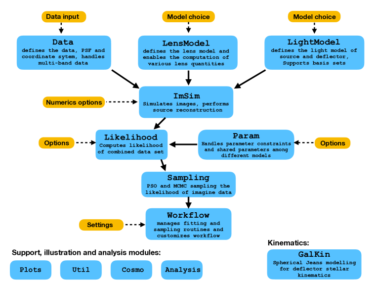
Figure 1: The lenstronomy hierarchical structure of the core modules. Arrow mark the dependencies and interfaces between the different modules. Orange boxes mark user API’s.

In Section 3, we briefly describe the main functionalities of the core modules and provide some simple use cases. The interplay between the modules is demonstrated in Section 4 and 5.

3 Core modules of lenstronomy

In the following, we describe the basic functionalities of the most important modules of lenstronomy with some simple examples. More detailed information about the available routines and their use can be accessed through the online documentation.

3.1 LensModel module

LensModel and its sub-packages execute all the purely lensing related tasks of lenstronomy. This includes ray-shooting, solving the lens equation, arrival time computation and non-linear solvers to optimize lens models for specific image configurations. The module allows consistent integration with single and multi plane lensing and an arbitrary superpositions of lens models. There is a wide range of lens models available. For details we refer the reader to the online-documentation.

To demonstrate the design of LensModel, we initialize a lens model and then execute some lensing calculations. First, we perform these calculations in a single-plane configuration 3.1.1 and then in a multi-plane configuration 3.1.2. Then we demonstrate the lens equation solver, that can be applied in both cases with the same API 3.1.3.

3.1.1 Single-plane lensing

The default setting of LensModel is to operate in single lens plane mode, where the superpositions of multiple lens models are de-coupled. Below we provide and example of a lens model, that consists of a super-position of an elliptical power-law potential, an external shear and an additional singular isothermal sphere perturber. We initialize the LensModel class, define the parameters for each individual model and perform some standard lensing calculations, such as a backwards ray-shooting of an image plane coordinate, computation of the Fermat potential and evaluating the magnification.

⬇

1# import the LensModel class #

2from lenstronomy.LensModel.lens_model import LensModel

3

4# specify the choice of lens models #

5lens_model_list = [’SPEP’, ’SHEAR’, ’SIS’]

6

7# setup lens model class with the list of lens models #

8lensModel = LensModel(lens_model_list=lens_model_list)

9

10# define parameter values of lens models #

11kwargs_spep = {’theta_E’: .9, ’e1’: 0.05, ’e2’: 0.05, ’gamma’: 2., ’center_x’: 0.1, ’center_y’: 0}

12kwargs_shear = {’e1’: 0.05, ’e2’: 0.0}

13kwargs_sis = {’theta_E’: 0.1, ’center_x’: 1., ’center_y’: -0.1}

14kwargs_lens = [kwargs_spep, kwargs_shear, kwargs_sis]

15

16# image plane coordinate #

17theta_ra, theta_dec = .9, .4

18

19# source plane coordinate #

20beta_ra, beta_dec = lensModel.ray_shooting(theta_ra, theta_dec, kwargs_lens)

21# Fermat potential #

22fermat_pot = lensModel.fermat_potential(x_image=theta_ra, y_image=theta_dec, x_source=beta_ra, y_source=beta_dec, kwargs_lens=kwargs_lens)

23

24# Magnification #

25mag = lensModel.magnification(theta_ra, theta_dec, kwargs_lens)

Additionally, the LensModel class allows to compute the Hessian matrix, shear and convergence, deflection angle and lensing potential. These routines are fully compatible with the numpy array structure and superposition of an arbitrary number of lens models.

3.1.2 Multi-plane lensing

The multi-plane setting of LensModel allows the user to place several deflectors at different redshifts. When not further specified, the default cosmology used is that of the astropy cosmology class. The API to access the lensing functionalities remains the same as for the single-plane setting 3.1.1. As an example, we take the same setting as in 3.1.1 but place the singular isothermal sphere perturber at a lower redshift.

⬇

1# keep the imports and variables from above #

2# specify redshifts of deflectors #

3redshift_list = [0.5, 0.5,.1]

4# specify source redshift #

5z_source = 1.5

6# setup lens model class with the list of lens models #

7lensModel_mp = LensModel(lens_model_list=lens_model_list, z_source=z_source, redshift_list=redshift_list, multi_plane=True)

8

9# source plane coordinate #

10beta_ra, beta_dec = lensModel_mp.ray_shooting(theta_ra, theta_dec, kwargs_lens)

11

12# Magnification #

13mag = lensModel_mp.magnification(theta_ra, theta_dec, kwargs_lens)

3.1.3 Lens equation solver

Solving the lens equation to compute the (multiple) image positions of a given source position can be conveniently performed within LensModel and is supported with a general instance of the LensModel class.

⬇

1# keep the imports and variables from above #

2# import the lens equation solver class #

3from lenstronomy.LensModel.Solver.lens_equation_solver import LensEquationSolver

4

5# specifiy the lens model class to deal with #

6solver = LensEquationSolver(lensModel)

7

8# solve for image positions provided a lens model and the source position #

9theta_ra, theta_dec = solver.image_position_from_source(beta_ra, beta_dec, kwargs_lens)

10

11# the magnification of the point source images #

12mag = lensModel.magnification(theta_ra, theta_dec, kwargs_lens)

Two lens models are shown in Figure 2. The source position of the example and the solutions of the lens equation (image positions) are marked.

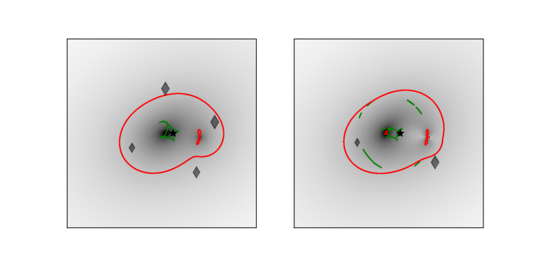
Figure 2: Illustrations of the two lens models created in Section 3.1. Left: The single-plane lens model of 3.1.1. Right: The multi-plane lens model of 3.1.2. In gray-scale the convergence map of the lens models, red lines correspond to the critical curve, green lines to the caustics. The green star corresponds to the source positions and the diamonds to the corresponding image positions.

3.2 LightModel module

The LightModel class provides the functionality to describe galaxy surface brightnesses. LightModel supports various analytic profiles as well as representations in shapelet basis sets. Any superposition of different profiles is supported. We refer to the online documentation for the full list of surface brightness profiles available and their parameterisation.

As an example, we initialize two LightModel class, one with a spherical Sersic profile and one with an elliptical Sersic profile. We define the profile parameters and evaluate the surface brightness at a specific position. The two LightModel instances will later be used as the lens light and the source light.

⬇

1# import the LightModel class #

2from lenstronomy.LightModel.light_model import LightModel

3# set up the list of light models to be used #

4source_light_model_list = [’SERSIC’]

5lightModel_source = LightModel(light_model_list=source_light_model_list)

6lens_light_model_list = [’SERSIC_ELLIPSE’]

7lightModel_lens = LightModel(light_model_list=lens_light_model_list)

8# define the parameters #

9kwargs_light_source = [{’I0_sersic’: 10, ’R_sersic’: 0.02, ’n_sersic’: 1.5, ’center_x’: beta_ra, ’center_y’: beta_dec}]

10# ellipticity parameter are defined as eccentricities #

11import lenstronomy.Util.param_util as param_util

12e1, e2 = param_util.phi_q2_ellipticity(phi=0.5, q=0.7)

13kwargs_light_lens = [{’I0_sersic’: 1000, ’R_sersic’: 0.1, ’n_sersic’: 2.5, ’e1’: e1, ’e2’: e2, ’center_x’: 0.1, ’center_y’: 0}]

14

15# evaluate surface brightness at a specific position #

16flux = lightModel_lens.surface_brightness(x=1, y=1, kwargs_list=kwargs_light_lens)

3.3 PointSource module

To accurately predict and model the positions and fluxes of point sources, different numerical procedures are needed compared to extended surface brightness features. The PointSource module manages the different options in describing point sources (e.g. in the image plane or source plane, with fixed magnification or allowed with individual variations thereof) and provides a homogeneous API to access image positions and magnifications. The PointSource class requires an instance of a LensModel class in case of lensed sources and arbitrary superpositions of point sources are allowed.

In the example below, we create two instances of the PointSource class. One with a parameterization in the source plane and one with a parameterization in the image plane. The API to access the necessary information about the image positions and magnifications remain the same in both cases.

⬇

1# import the PointSource class #

2from lenstronomy.PointSource.point_source import PointSource

3

4# unlensed source positon #

5point_source_model_list = [’SOURCE_POSITION’]

6pointSource = PointSource(point_source_type_list=point_source_model_list, lensModel=lensModel, fixed_magnification_list=[True])

7kwargs_ps = [{’ra_source’: beta_ra, ’dec_source’: beta_dec, ’source_amp’: 100}]

8# return image positions and amplitudes #

9x_pos, y_pos = pointSource.image_position(kwargs_ps=kwargs_ps, kwargs_lens=kwargs_lens)

10point_amp = pointSource.image_amplitude(kwargs_ps=kwargs_ps, kwargs_lens=kwargs_lens)

11

12# lensed image positions (solution of the lens equation) #

13point_source_model_list = [’LENSED_POSITION’]

14pointSource = PointSource(point_source_type_list=point_source_model_list, lensModel=lensModel, fixed_magnification_list=[False])

15kwargs_ps = [{’ra_image’: theta_ra, ’dec_image’: theta_dec, ’point_amp’: np.abs(mag)*30}]

16# return image positions and amplitudes #

17x_pos, y_pos = pointSource.image_position(kwargs_ps=kwargs_ps, kwargs_lens=kwargs_lens)

18point_amp = pointSource.image_amplitude(kwargs_ps=kwargs_ps, kwargs_lens=kwargs_lens)

3.4 Data module

The Data module consists of two main classes. The Data class stores and manages all the imaging data relevant information. This includes the coordinate frame, coordinate-to-pixel transformation (and the inverse), and, in the case of fitting, also noise properties for computing the likelihood of the data given the model. The PSF class handles the point spread function convolution. Supported are pixelised convolution kernels as well as some analytic profiles.

⬇

1# import the Data() class #

2from lenstronomy.Data.imaging_data import Data

3deltaPix = 0.05 # size of pixel in angular coordinates #

4

5# setup the keyword arguments to create the Data() class #

6kwargs_data = {’numPix’: 100,

7 ’ra_at_xy_0’: -2.5,

8 ’dec_at_xy_0’: -2.5,

9 ’transform_pix2angle’: np.array([[1, 0], [0, 1]]) * deltaPix}

10data = Data(kwargs_data)

11# return the list of pixel coordinates #

12x_coords, y_coords = data.coordinates

13# compute pixel value of a coordinate position #

14x_pos, y_pos = data.map_coord2pix(ra=0, dec=0)

15# compute the coordinate value of a pixel position #

16ra_pos, dec_pos = data.map_pix2coord(x=20, y=10)

17

18# import the PSF() class #

19from lenstronomy.Data.psf import PSF

20kwargs_psf = {’psf_type’: ’GAUSSIAN’, ’fwhm’: 0.1, ’pixel_size’: deltaPix}

21psf = PSF(kwargs_psf)

22# return the pixel kernel corresponding to a point source #

23kernel = psf.kernel_point_source

3.5 ImSim module

At the core of the IMSim module is the ImageModel class. ImageModel is the interface to combine all the different components, LensModel, LightModel, PointSource and Data to model images. The LightModel can be used to model both lens light (un-lensed) and source light (lensed) components. ImSim supports all functionalities of each of those components. ImageModel is supported by the class ImageNumerics that specifies and executes the numerical options accessible. Among the numerical options are sub-pixel grid resolution ray-tracing and convolutions that can improve numerical accuracy in the presence of either small lensing perturbations and/or a highly variable surface brightness profile (see e.g. Tessore et al., 2016, for the latter).

3.5.1 Image simulation

As an example, we simulate an image with an instance of ImageModel that use instances of the classes we created above. We can define two different LightModel instances for the lens and source light. We define the sub-pixel ray-tracing resolution and whether the PSF convolution is applied on the higher resolution ray-tracing grid or on the degraded pixel image.

⬇

1# import the ImageModel class #

2from lenstronomy.ImSim.image_model import ImageModel

3# define the numerics #

4kwargs_numerics = {’subgrid_res’: 3,

5 ’psf_subgrid’: True}

6# initialize the Image model class by combining the modules we created above #

7imageModel = ImageModel(data_class=data, psf_class=psf, lens_model_class=lensModel,

8 source_model_class=lightModel_source,

9 lens_light_model_class=lightModel_lens,

10 point_source_class=pointSource,

11 kwargs_numerics=kwargs_numerics)

12# simulate image with the parameters we have defined above #

13image = imageModel.image(kwargs_lens=kwargs_lens, kwargs_source=kwargs_light_source,

14 kwargs_lens_light=kwargs_light_lens, kwargs_ps=kwargs_ps)

15

16# we can also add noise #

17import lenstronomy.Util.image_util as image_util

18# exposure time to quantify the Poisson noise level #

19exp_time = 100

20# background rms value #

21background_rms = 0.1

22poisson = image_util.add_poisson(image, exp_time=exp_time)

23bkg = image_util.add_background(image, sigma_bkd=background_rms)

24image_noisy = image + bkg + poisson

Figure 3 shows the simulated image of the example computed above with the single-plane lens model of Section 3.1.1 (left panel) and for the same Sersic light profiles but with the multi-plane lens model of Section 3.1.2 in the right panel. To illustrate the numerical procedure in how lenstronomy renders images, we provide another example consisting of a high resolution galaxy profile in Figure 4.

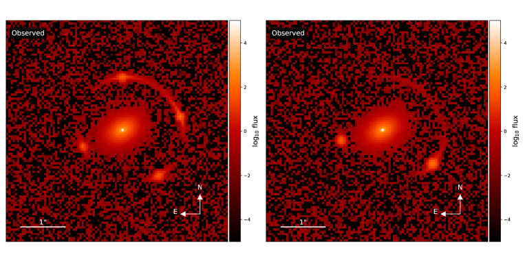
Figure 3: Simulated images with the chosen options of the ImageModel class (3.5). Left: The single-plane lens model results in a quadruply imaged quasar. Right: The multi-plane model results in a double lensed quasar.

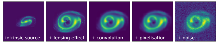
Figure 4: Illustration of the sequence of steps performed by the ImSim module. From left to right: A galaxy described with a high resolution shapelet representation (1), seen through gravitational lensing, i.e. evaluated in the image plane coordinates (2), convolved on a subpixel high resolution grid (3), down-graded to pixel resolution and added with noise (5).

3.5.2 Linear inversion

Parameters corresponding to an an amplitude of a surface brightness distribution have a linear response on the predicted flux values of pixels and can be inferred by a linear minimization based on the data (Warren and Dye, 2003). lenstronomy automatically identifies those parameters. The ImSim module comes with an option such that the linear parameters do not have to be provided when fitting a model to data. This can reduce the number of non-linear parameters significantly, depending on the source complexity to be modelled. In the example provided in Section 3.5.1, we have 6 linear parameters, the 4 point source amplitudes and the amplitudes of the Sersic profile of the lens and source. To perform the linear inversion, noise properties of the data have to be known or assumed (see Section 3.5.3). There are different approaches in the literature that perform different types of semi-linear inversions (e.g. Suyu et al., 2006; Vegetti and Koopmans, 2009; Tagore and Keeton, 2014; Birrer et al., 2015; Nightingale and Dye, 2015).

In the example below, we add the noisy data to the ImageModel instance, then delete the knowledge about the linear parameters and solve for the linear coefficients based on the data.

⬇

1# update the data with the noisy image and its noise properties #

2kwargs_data[’image_data’] = image_noisy

3kwargs_data[’background_rms’] = background_rms

4kwargs_data[’exposure_map’] = np.ones_like(image_noisy)* exp_time

5data_class_sim = Data(kwargs_data)

6imageModel.update_data(data_class_sim)

7

8# we do not require the knowledge of the linear parameters #

9del kwargs_light_source[0][’amp’]

10# apply the linear inversion to fit for the noisy image #

11image_reconstructed, _, _, _ = imageModel.image_linear_solve(kwargs_lens=kwargs_lens, kwargs_source=kwargs_light_source, kwargs_lens_light=kwargs_light_lens, kwargs_ps=kwargs_ps)

3.5.3 Likelihood definition

The likelihood of the data given a model $p(d_{\text{data}}|d_{\text{model}})$ is key in sampling the parameter posterior distribution (Section 3.6) and also to perform the linear inversion (Section 3.5.2). The convention lenstronomy uses to compute $p(d_{\text{data}}|d_{\text{model}})$ is

$$\log p(d_{\text{data}}|d_{\text{model}})=\sum_{i}\frac{(d_{\text{data,i}}-d_{\text{model,i}})^{2}}{2\sigma_{\text{i}}^{2}}+\text{const}.$$ (1)

The constant term in equation 1 is not computed by lenstronomy. The error in each pixel, $\sigma_{\text{i}}$, consists of a Gaussian background term, $\sigma_{\text{bkg}}$, and a Poisson term based on the count statistics of an individual pixel, $f_{i}$, such that $d_{\text{model,i}}/f_{i}$ is the Poisson error predicted by the model in the time units of the data, and writes

$$\sigma_{i}^{2}=\sigma_{\text{bkgd}}^{2}+d_{\text{model,i}}/f_{i}.$$ (2)

In our example of 3.5.1, $f_{i}$ is the exposure time for each pixel and $\sigma_{\text{bkgd}}$ is the background rms value. CCD gain and other components may be incorporated into $f_{i}$.

The linear inversion requires an estimate of the noise term, $\sigma_{i}^{2}$, without the knowledge of the model, $d_{\text{model,i}}$. For this particular step, the linear inversion is performed based on the Poisson noise expected by the data itself

$$\sigma_{\text{linear, i}}^{2}=\sigma_{\text{bkgd}}^{2}+d_{\text{data,i}}/f_{i}.$$ (3)

The analytic marginalization over the covariance matrix of the linear inversion (Gaussian approximation) can be added (see Birrer et al., 2015, for further information). Additionally, pixel masks can be set and additional error terms can be plugged in, if required. lenstronomy provides a direct access to the likelihood of the data given a model and performs all the required computations:

⬇

1logL = imageModel.likelihood_data_given_model(kwargs_lens,kwargs_light_source,kwargs_light_lens,kwargs_ps)

3.6 Sampling module

The Sampling module manages the execution of the non-linear fitter (e.g. PSO) and the parameter inference (e.g. emcee). The module is built up such that the user can plug in their own customized sampler. The Sampling Module consists of three major classes: The Likelihood class manages the specific likelihood function, consisting of the imaging likelihood and potential other data and constraints and provides the interface to the sampling routines. The Param class handles all the model choices and the parameters going in it and supports the Likelihood class. Together they handle all the model choices of the user and mitigate them to the external modules and from the external modules back to lenstronomy. Finally, the Sampler class gives specific examples how the Likelihood class can be used to execute specific samplers.

3.6.1 Parameter handling

External sampling modules require a likelihood function that is consistent with their own parameter handling, mostly in ordered arrays. The likelihood in Section 3.5.3 requires lenstronomy conventions in terms of lists of keyword arguments. The Param class is the API of the lenstronomy conventions of parameters used in the ImSim module and the standardized parameter arrays used by external samplers (such as CosmoHammer or emcee). The Param class enables the user further to set options:

1. keep certain parameters fixed

2. handling of the linear parameters

3. provide additional constraints on the modelling (e.g. fix source profile to point source position etc.)

Below we provide an example where initialize a Param class consistent with the options chosen in the previous sections and where we specify fixed and joint parameters. We then perform the mapping between lenstronomy conventions and formats being used by external sampling modules.

⬇

1# import the parameter handling class #

2from lenstronomy.Sampling.parameters import Param

3# set options for constraint parameters #

4kwargs_constraints = {

5 ’num_point_source_list’: [4], # when modelling a doube, use [2]

6 ’joint_source_with_point_source’: [[0, 0]],

7 ’solver’: True,

8 ’solver_type’: ’PROFILE_SHEAR’, # ’PROFILE’, ’PROFILE_SHEAR’, ’ELLIPSE’, ’CENTER’

9 }

10# list fixed parameters #

11kwargs_fixed_lens = [{’gamma’: 2.}, {}, {}]

12kwargs_fixed_source = [{}]

13kwargs_fixed_lens_light = [{}]

14kwargs_fixed_ps = [{}]

15

16# make instance of parameter class with given model options, constraints and fixed parameters #

17param = Param(kwargs_model, kwargs_constraints, kwargs_fixed_lens, kwargs_fixed_source,

18 kwargs_fixed_lens_light, kwargs_fixed_ps, kwargs_lens_init=kwargs_lens)

19

20# the number of non-linear parameters and their names #

21num_param, param_list = param.num_param()

22

23# parameter array for fitting routine #

24param_array = param.setParams(kwargs_lens, kwargs_light_source, kwargs_light_lens, kwargs_ps)

25

26# recover keyword arguments list for lenstronomy from a parameter array of the fitting routine #

27kwargs_lens_out, kwargs_light_source_out, kwargs_light_lens_out, kwargs_ps_out, _ = param.getParams(param_array)

28

29# print settings #

30param.print_setting()

3.6.2 Likelihood execution

The Likelihood class combines the ImSim module and the Param class to allow a direct access to the lenstronomy likelihood from an external sampler. In addition, the Likelihood class allows to a simultaneous handling of multi-band data and to incorporate other data, such as time-delay measurements. Below we initialize a Likelihood class and execute the likelihood function from an ordered array of parameters.

⬇

1# define options of the likelihood #

2kwargs_likelihood = {’source_marg’: False,

3 ’check_solver’: True,

4 ’solver_tolerance’: 0.001,}

5

6# import the likelihood class #

7from lenstronomy.Sampling.likelihood import LikelihoodModule

8

9# make instance of the likelihood class #

10likelihoodModule = LikelihoodModule(imSim_class=imageModel, param_class=param, kwargs_likelihood=kwargs_likelihood)

11

12# execute the likelihood from an ordered parameter array #

13logL = likelihoodModule.logL(args=param_array)

3.6.3 Sampling the parameter space

The Sampler class consists of examples of different samplers that can be used. As an example, we run a Particle Swarm Optimization (PSO) with the previous instance of the Likelihood class.

⬇

1# initial guess of non-linear parameters, we chose different starting parameters than the truth #

2kwargs_lens_init = [{’theta_E’: 1.2, ’e1’: 0, ’e2’: 0, ’gamma’: 2., ’center_x’: 0., ’center_y’: 0},

3 {’e1’: 0.0, ’e2’: 0.01}, {’theta_E’: 0.1, ’center_x’: 1., ’center_y’: 0}]

4kwargs_source_init = [{’R_sersic’: 0.03, ’n_sersic’: 1., ’center_x’: 0, ’center_y’: 0}]

5kwargs_lens_light_init = [{’R_sersic’: 0.1, ’n_sersic’: 1, ’e1’: 0, ’e2’: 0, ’center_x’: 0, ’center_y’: 0}]

6kwargs_ps_init = [{’ra_image’: theta_ra+0.01, ’dec_image’: theta_dec-0.01}]

7

8# initial spread in parameter estimation #

9kwargs_lens_sigma = [{’theta_E’: 0.3, ’e1’: 0.5, ’e2’: 0.5, ’gamma’: .2, ’center_x’: 0.1, ’center_y’: 0.1},

10 {’e1’: 0.1, ’e2’: 0.1}, {’theta_E’: 0.1, ’center_x’: .1, ’center_y’: 0.1}]

11kwargs_source_sigma = [{’R_sersic’: 0.1, ’n_sersic’: .5, ’center_x’: .1, ’center_y’: 0.1}]

12kwargs_lens_light_sigma = [{’R_sersic’: 0.1, ’n_sersic’: 0.2, ’e1’: 0.2, ’e2’: 0.2, ’center_x’: .1, ’center_y’: 0.1}]

13kwargs_ps_sigma = [{’ra_image’: [0.02] * 4, ’dec_image’: [0.02] * 4}]

14

15# ordered array for sampler #

16param_init = param.setParams(kwargs_lens_init, kwargs_source_init, kwargs_lens_light_init, kwargs_ps_init)

17param_sigma = param.setParams(kwargs_lens_sigma, kwargs_source_sigma, kwargs_lens_light_sigma, kwargs_ps_sigma)

18

19# upper and lower range to initialise the sampler #

20upper_start = np.array(param_init) + np.array(param_sigma)

21lower_start = np.array(param_init) - np.array(param_sigma)

22

23# import the sampling class #

24from lenstronomy.Sampling.sampler import Sampler

25# initialize the Sampler class with the likelihoodModule #

26sampler = Sampler(likelihoodModule=likelihoodModule)

27

28# execute a PSO from the Sampler #

29result, chain_properties = sampler.pso(n_particles=200, n_iterations=200, lower_start=lower_start, upper_start=upper_start)

30

31# cast result back in lenstronomy conventions #

32lens_result, source_result, lens_light_result, ps_result, _ = param.getParams(result)

Additionally to the example mentioned above, hard bounds on the upper and lower range in parameter space can be provided.

3.7 Workflow module

The Workflow module allows the user to perform a sequence of PSO and/or MCMC runs. The user can run the sequence of fitting routines with taking the results of the previous routine as an input of the next one. The user can specify (optionally) to keep one or multiple parameter classes (lens model, source model, lens light model and source model) fixed during the fitting process of individual runs. Iterative PSF optimization can also be injected within the fitting sequence. The FittingSequence class enables a reliable execution of tasks on non-local platforms, such as hight performance clusters and supports parallel executions of likelihood evaluations with the MPI portocoll built in CosmoHammer (Akeret et al., 2013).

3.8 GalKin module

Kinematics of the lensing galaxy can provide additional constraints on the lens model and can help to reduce systematics inherent in lensing. The GalKin module provides the support to self-consistently model and predict the velocity dispersion of the lensing galaxy given the surface brightness profile and the lens model upon which the image modelling consists of. The kinematics require the knowledge/assumption of the 3d light and mass profiles. Not all lens and light models can be analytically de-projected. In these cases, lenstronomy performs a Multi-Gaussian decomposition (Cappellari, 2002) and the de-projection is performed on the individual Gaussian components. The kinematics is computed with spherical Jeans anisotropy modelling (JAM). lenstronomy supports the stellar anisotropy profiles described in Mamon and Łokas (2005). Observational conditions, i.e. the PSF and the aperture are modelled with a spectral rendering approach described in Birrer et al. (2017a).

4 Modelling examples

The design of lenstronomy and the core modules described in Section 3 allow a wide range of modelling tasks to be executed. We demonstrated in the previous section how to combine the modules to enable a joint sampling of point source, extended source, lens light and lens deflector model. In this section, we provide five examples in different sub-domains where we demonstrate the capabilities of lenstronomy, source reconstruction 4.1, image de-convolution 4.2, galaxy structural analysis 4.3, quasar-host galaxy decomposition 4.4 and multiband fitting 4.5. Detailed example workflows for the different applications are presented in the online documentation.

4.1 Source reconstruction

Reconstruction techniques are required to describe the source morphology at the scales relevant for given data. The needed complexity may strongly depend on the type of galaxy being lensed and the resolution and signal-to-noise of the data. In Figure 5, we provide an example where we reconstruct a source galaxy with complex morphology with a Shapelet basis set with maximum polynomial order, $n_{\text{max}}=29$. We are able to represent the features present in the image. The reconstruction of the source reproduces the macroscopic morphology of the input galaxy.

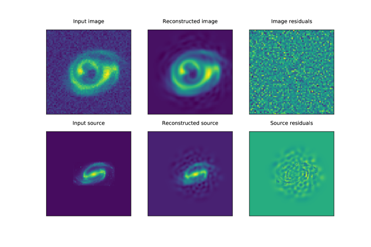
Figure 5: lenstronomy source reconstruction capabilities (de-lensing + de-convolution). Top: Image plane. bottom: Source plane. From left to right: The simulated image with noise based on a realistic galaxy surface brightness profile (same example as Figure 4) (1), the reconstruction by the linear inversion technique based on a lower resolution shapelet basis set (2), the residuals of the input relative to the reconstructed model. The lens model was kept fixed to the input model for the reconstruction.

lenstronomysupports a wide range in models and also allows to superpose analytical models with basis sets (see e.g. Birrer et al., 2018b). The reconstruction for a given set of lens and light model parameters is performed by the linear lens inversion (Section 3.5.2). lenstronomy does not provide a Bayesian evidence optimization itself, but this can be performed by the user in post-processing (e.g. Birrer et al., 2018b). The performance of the source reconstruction capabilities has been compared with the SLIT software (Joseph et al., 2018) and was found to behave well in speed and reconstruction accuracy.

4.2 Image de-convolution

The source reconstruction in Section 4.1 is a combination of two distinct steps: a de-lensing (effectively a non-linear mapping between the image plane and the basis set represented in the source plane) and a de-convolution. By removing the class instance of LensModel from the ImSim module or by removing all the lens models, the linear inversion method built in lenstronomy effectively performs a de-convolution. This is demonstrated in Figure 6 where we take a scaled version of the same galaxy as for Figure 5 with a PSF convolution kernel and apply the same shapelet basis set to describe the image.

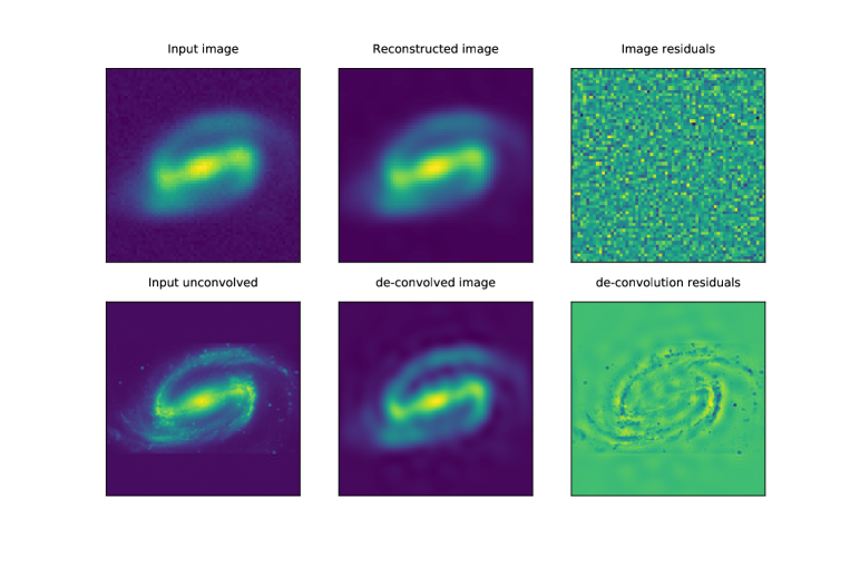
Figure 6: lenstronomy de-convolution capabilities (source reconstruction without lensing). Top: Convolved images. bottom: Unconvolved images. From left to right: The simulated image with noise based on a realistic galaxy surface brightness profile (same example as Figure 4 but scaled and with a larger convolution kernel applied) (1), the reconstruction by the linear inversion technique based on a lower resolution shapelet basis set (2), the residuals of the input relative to the reconstructed model.

4.3 Galaxy structural analysis

lenstronomy can be used to extract structural components from galaxy images. This is yet another example where the lensing capabilities of lenstronomy do not have to be used necessarily. In terms of flexibility, lenstronomy contains similar features as the well established software GALFIT (Peng et al., 2002, 2010). lenstronomy provides an open source alternative in python. We also emphasize that lenstronomy comes along with an MCMC algorithm that can provide covariances between inferred parameters. Additionally, lenstronomy is able to extract structural parameters from lensed and highly distorted galaxies.

4.4 Quasar-host galaxy decomposition

In the case where the galaxy contains a quasar, simultaneous decompositions of the host galaxy and a point source component can be performed with lenstronomy. Figure 7 demonstrates this capability. A joint fitting of two component Sersic profile for the host galaxy and a quasar point source were used as an input model and the different components were recovered in the modelling.

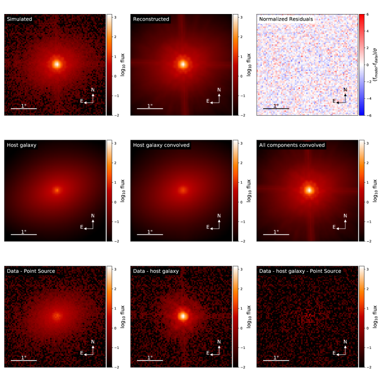
Figure 7: Illustration of the lenstronomy quasar-host galaxy decomposition capabilities. A two-component host galaxy is modelled with a significantly brighter quasar at its center. lenstronomy can reliably decompose the two components. Top: Simulated image (left), reconstructed model (middle) and residuals of the reconstruction (right). Middle: The separation of the model components. Bottom: The subtraction of the model components from the data.

4.5 Multiband fitting

lenstronomy is explicitly designed to simultaneously model lenses in multiple imaging bands. The coordinate system definition is image independent and can be shared among multiple data sets. The ImSim module (see 3.5) contains a class Multiband that naturally handles an arbitrary number of data sets, all with their own descriptions (see 3.4). The Multiband class shares the same API as the ImageModel class for single images and thus allows to be used with the Sampling and Workflow modules. The non-linear parameters, such as lens model, point source position and light profile shapes are shared among the different bands. The linear parameters, however, are optimized for each band individually. This allows e.g. for different galaxy morphologies in different wavelength. The multi-band approach allows also to model a set of single exposures directly rather than rely on combined post-processed data products. This approach can also be used to model disjoint patches of a cluster arc without requiring a large image.

Precise relative astrometry may be required to perform the lens modelling in a joint coordinate frame. lenstronomy comes with an iterative routine to align coordinate frames from different bands given a shared model description. This can be used to align images to determine e.g. a point source or the lensing galaxy light center.

5 Science applications of lenstronomy

In this section we provide science examples that lenstronomy has enabled. In particular, we will highlight specific settings within lenstronomy that were required to conduct the analysis in the domain of substructure lensing, time-delay cosmography and cosmic shear measurements.

As the size and diversity of known strong lensing systems increases, a wider variety of science topics can be tackled, such as time-delay cosmography with lensed SNIa Grillo et al. (2018), single star micro-lensing cluster arcs Kelly et al. (2018), double source-plane cosmography Gavazzi et al. (2008); Collett and Auger (2014) or cosmic shear measurements with Einstein rings (Birrer et al., 2018a).

We emphasize that the choices when modelling a specific system remains the task of the user. lenstronomy may facilitate scientific analysis of strong lenses, but should be accompanied by rigorous testing of the specific method applied, desirably through simulations. lenstronomy allows to simulate accurate mock data with very complex structure in lens and source and therefore facilitate the exploration of systematics in the analysis.

5.1 Lensing substructure quantification

Modeling substructure within a deflector can be done by combining multiple lens models (e.g. a main deflector, external shear and a small clump) within one instance of LensModel (Section 3.1). Substructure can be represented by a NFW profile, truncated NFW profile or a variety of other profiles implemented in lenstronomy. A superposition of an arbitrary number of lens profiles based on a mass function is possible and has been used by Gilman et al. (2018). The multi-plane setting also allows to model the full line-of-sight contribution of field halos.

Lensing substructure is expected to perturb the deflection angles at the milliarcsecond scale, which is e.g. below the pixel resolution of an HST image. To detect and/or quantify those astrometric anomalies, the numerical description in the modelling must accurately capture these small effects. Sub-grid resolution ray-tracing is required to perform such analysis on HST images. Accuracy comes with a computational cost and lenstronomy enables the user to set the right numerical description for the problem in hand.

Additionally, the source surface brightness resolution captured by the model must be sufficiently high resolution not to falsely attribute residuals in the image reconstruction to lensing substructure when they originate from missing scales in the source reconstruction. In Birrer et al. (2017a), we specifically enhanced the source reconstruction resolution where we proposed a clump to be present.

5.2 Time-delay cosmography

The workflow API facilitates a fast exploration of various choices and options in all the aspects of lens modelling. It is necessary to explore the degeneracies inherent in lensing and their impact on the cosmographic inference. In Birrer et al. (2016), we explored the source scale degeneracy by explicitly mapping out the source size with the shapelet scale parameter. In Birrer et al. (2018b) we combined 128 different model settings based on their relative Bayesian Information Criteria to provide a posterior distribution reflecting uncertainties in the model choices. The built-in time-delay likelihood and the GalKin module provide the full support for a fully self-consistent analysis of imaging, time-delay and kinematic data to derive cosmographic constraints.

5.3 Cosmic shear measurements

We applied lenstronomy to model and reconstruct the non-linear shear distortions that couple to the main deflector in an Einstein ring lens in the COSMOS field (Birrer et al., 2017b). The detailed modelling of the HST imaging of the Einstein ring allowed us to constrain the shear parameters to very high precision. lenstronomy is aimed to have the flexibility to model hundreds or even the aimed thousands of Einstein ring lenses expected in future space based surveys to provide comparable and complementary cosmic shear measurements, as been fore-casted by Birrer et al. (2018a).

6 Conclusion

We have presented lenstronomy , a multi-purpose open source lens modelling software package in python. We outlined its design and the major supported features. lenstronomy has been used to study the expansion history of the universe with time-delay cosmography and to probe dark matter properties by substructure lensing. The modular nature of lenstronomy provides support for a wide range of scientific studies. We have provided modelling and science examples to illustrate some of the capabilities of lenstronomy . The software is distributed under the MIT license. The software is actively used and maintained and the latest stable release will be distributed through the python packaging index. We refer to the online documentation, where the latest starter guide, example notebooks, source code and installation guidelines can be found.

Appendix A Publicly available lens modelling software

A collection of public available lens modelling software presented in the literature is listed below. We refer to specific literature and online documentations for the scope of each individual software and its current development status.

• gravlens (Keeton, 2011): A standard lens model software widely used in the community. Includes a wide range of basic lensing calculations and comes with an extension that adds many routines for modeling strong lenses.

• lenstool (Kneib et al., 2011): A lensing software for modeling mass distribution of galaxies and clusters. Comes with a Bayesian inference method.

• PixeLens (Saha and Williams, 2011): A program for reconstructing gravitational lenses from multiple-imaged point sources. It can explore ensembles of lens-models consistent with given data on several different lens systems at once.

• glafic (Oguri, 2010): Support for many mass models and parametric light models. Simulats lensed extended images with PSF convolution.

• LENSED (Tessore et al., 2016): Performs forward parametric modelling of strong lenses. Supports computing on GPUs.

• AutoLens (Nightingale et al., 2018): An automated modeling suite for the analysis of galaxy-scale strong gravitational lenses. Incorporates an adaptive grid source reconstruction technique.

• Ensai (Hezaveh et al., 2017): Estimating parameters of strong gravitational lenses with convolutional neural networks.

• pySPT (Wertz and Orthen, 2018): A package dedicated to the Source Position Transformation (SPT). The main goal of pySPT is to provide a tool to quantify the systematic errors that are introduced by the SPT in lens modeling.

References

- Agnello et al. (2015) Agnello, A., Treu, T., Ostrovski, F., Schechter, P. L., Buckley-Geer, E. J., Lin, H., Auger, M. W., Courbin, F., Fassnacht, C. D., Frieman, J., Kuropatkin, N., Marshall, P. J., McMahon, R. G., Meylan, G., More, A., Suyu, S. H., Rusu, C. E., Finley, D., Abbott, T., Abdalla, F. B., Allam, S., Annis, J., Banerji, M., Benoit-Lévy, A., Bertin, E., Brooks, D., Burke, D. L., Carnero Rosell, A., Carrasco Kind, M., Carretero, J., Cunha, C. E., D’Andrea, C. B., da Costa, L. N., Desai, S., Diehl, H. T., Dietrich, J. P., Doel, P., Eifler, T. F., Estrada, J., Fausti Neto, A., Flaugher, B., Fosalba, P., Gerdes, D. W., Gruen, D., Gutierrez, G., Honscheid, K., James, D. J., Kuehn, K., Lahav, O., Lima, M., Maia, M. A. G., March, M., Marshall, J. L., Martini, P., Melchior, P., Miller, C. J., Miquel, R., Nichol, R. C., Ogando, R., Plazas, A. A., Reil, K., Romer, A. K., Roodman, A., Sako, M., Sanchez, E., Santiago, B., Scarpine, V., Schubnell, M., Sevilla-Noarbe, I., Smith, R. C., Soares-Santos, M., Sobreira, F., Suchyta, E., Swanson, M. E. C., Tarle, G., Thaler, J., Tucker, D., Walker, A. R., Wechsler, R. H., Zhang, Y., Dec. 2015. Discovery of two gravitationally lensed quasars in the Dark Energy Survey. MNRAS454, 1260–1265.
- Akeret et al. (2013) Akeret, J., Seehars, S., Amara, A., Refregier, A., Csillaghy, A., Aug. 2013. CosmoHammer: Cosmological parameter estimation with the MCMC Hammer. Astronomy and Computing 2, 27–39.
- Astropy Collaboration et al. (2013) Astropy Collaboration, Robitaille, T. P., Tollerud, E. J., Greenfield, P., Droettboom, M., Bray, E., Aldcroft, T., Davis, M., Ginsburg, A., Price-Whelan, A. M., Kerzendorf, W. E., Conley, A., Crighton, N., Barbary, K., Muna, D., Ferguson, H., Grollier, F., Parikh, M. M., Nair, P. H., Unther, H. M., Deil, C., Woillez, J., Conseil, S., Kramer, R., Turner, J. E. H., Singer, L., Fox, R., Weaver, B. A., Zabalza, V., Edwards, Z. I., Azalee Bostroem, K., Burke, D. J., Casey, A. R., Crawford, S. M., Dencheva, N., Ely, J., Jenness, T., Labrie, K., Lim, P. L., Pierfederici, F., Pontzen, A., Ptak, A., Refsdal, B., Servillat, M., Streicher, O., Oct. 2013. Astropy: A community Python package for astronomy. A&A558, A33.
- Birrer et al. (2015) Birrer, S., Amara, A., Refregier, A., Nov. 2015. Gravitational Lens Modeling with Basis Sets. ApJ813, 102.
- Birrer et al. (2016) Birrer, S., Amara, A., Refregier, A., Aug. 2016. The mass-sheet degeneracy and time-delay cosmography: analysis of the strong lens RXJ1131-1231. Journal of Cosmology and Astro-Particle Physics 2016, 020.
- Birrer et al. (2017a) Birrer, S., Amara, A., Refregier, A., May 2017a. Lensing substructure quantification in RXJ1131-1231: a 2 keV lower bound on dark matter thermal relic mass. Journal of Cosmology and Astro-Particle Physics 2017, 037.
- Birrer et al. (2018a) Birrer, S., Refregier, A., Amara, A., Jan. 2018a. Cosmic Shear with Einstein Rings. ApJ852, L14.
- Birrer et al. (2018b) Birrer, S., Treu, T., Rusu, C. E., Bonvin, V., Fassnacht, C. D., Chan, J. H. H., Agnello, A., Shajib, A. J., Chen, G. C. F., Auger, M., Courbin, F., Hilbert, S., Sluse, D., Suyu, S. H., Wong, K. C., Marshall, P., Lemaux, B. C., Meylan, G., Sep. 2018b. H0LiCOW - IX. Cosmographic analysis of the doubly imaged quasar SDSS 1206+4332 and a new measurement of the Hubble constant. ArXiv e-prints, arXiv:1809.01274.
- Birrer et al. (2017b) Birrer, S., Welschen, C., Amara, A., Refregier, A., Apr. 2017b. Line-of-sight effects in strong lensing: putting theory into practice. Journal of Cosmology and Astro-Particle Physics 2017, 049.
- Bonvin et al. (2017) Bonvin, V., Courbin, F., Suyu, S. H., Marshall, P. J., Rusu, C. E., Sluse, D., Tewes, M., Wong, K. C., Collett, T., Fassnacht, C. D., Treu, T., Auger, M. W., Hilbert, S., Koopmans, L. V. E., Meylan, G., Rumbaugh, N., Sonnenfeld, A., Spiniello, C., Mar. 2017. H0LiCOW - V. New COSMOGRAIL time delays of HE 0435-1223: H0 to 3.8 per cent precision from strong lensing in a flat CDM model. MNRAS465, 4914–4930.
- Cappellari (2002) Cappellari, M., Jun. 2002. Efficient multi-Gaussian expansion of galaxies. MNRAS333, 400–410.
- Collett and Auger (2014) Collett, T. E., Auger, M. W., Sep. 2014. Cosmological constraints from the double source plane lens SDSSJ0946+1006. MNRAS443, 969–976.
- Dalal and Kochanek (2002) Dalal, N., Kochanek, C. S., Jun. 2002. Direct Detection of Cold Dark Matter Substructure. ApJ572, 25–33.
- Ding et al. (2018) Ding, X., Treu, T., Shajib, A. J., Xu, D., Chen, G. C.-F., More, A., Despali, G., Frigo, M., Fassnacht, C. D., Gilman, D., Hilbert, S., Marshall, P. J., Sluse, D., Vegetti, S., Jan. 2018. Time Delay Lens Modeling Challenge: I. Experimental Design. ArXiv e-prints.
- Foreman-Mackey et al. (2013) Foreman-Mackey, D., Hogg, D. W., Lang, D., Goodman, J., Mar. 2013. emcee: The MCMC Hammer. PASP125, 306.
- Gavazzi et al. (2008) Gavazzi, R., Treu, T., Koopmans, L. V. E., Bolton, A. S., Moustakas, L. A., Burles, S., Marshall, P. J., Apr. 2008. The Sloan Lens ACS Survey. VI. Discovery and Analysis of a Double Einstein Ring. ApJ677, 1046–1059.
- Gilman et al. (2018) Gilman, D., Birrer, S., Treu, T., Keeton, C. R., Nierenberg, A., Nov. 2018. Probing the nature of dark matter by forward modelling flux ratios in strong gravitational lenses. MNRAS481, 819–834.
- Grillo et al. (2018) Grillo, C., Rosati, P., Suyu, S. H., Balestra, I., Caminha, G. B., Halkola, A., Kelly, P. L., Lombardi, M., Mercurio, A., Rodney, S. A., Treu, T., Jun. 2018. Measuring the Value of the Hubble Constant “à la Refsdal”. ApJ860, 94.
- Hezaveh et al. (2016) Hezaveh, Y. D., Dalal, N., Marrone, D. P., Mao, Y.-Y., Morningstar, W., Wen, D., Blandford, R. D., Carlstrom, J. E., Fassnacht, C. D., Holder, G. P., Kemball, A., Marshall, P. J., Murray, N., Perreault Levasseur, L., Vieira, J. D., Wechsler, R. H., May 2016. Detection of Lensing Substructure Using ALMA Observations of the Dusty Galaxy SDP.81. ApJ823, 37.
- Hezaveh et al. (2017) Hezaveh, Y. D., Levasseur, L. P., Marshall, P. J., Aug. 2017. Fast automated analysis of strong gravitational lenses with convolutional neural networks. Nature548, 555–557.
- Hunter (2007) Hunter, J. D., 2007. Matplotlib: A 2d graphics environment. Computing In Science & Engineering 9 (3), 90–95.
- Jacobs et al. (2017) Jacobs, C., Glazebrook, K., Collett, T., More, A., McCarthy, C., Oct. 2017. Finding strong lenses in CFHTLS using convolutional neural networks. MNRAS471, 167–181.
- Joseph et al. (2018) Joseph, R., Courbin, F., Starck, J. L., Birrer, S., Sep. 2018. Sparse Lens Inversion Technique (SLIT): lens and source separability from linear inversion of the source reconstruction problem. ArXiv e-prints, arXiv:1809.09121.
- Keeton (2011) Keeton, C. R., Feb. 2011. GRAVLENS: Computational Methods for Gravitational Lensing. Astrophysics Source Code Library.
- Kelly et al. (2018) Kelly, P. L., Diego, J. M., Rodney, S., Kaiser, N., Broadhurst, T., Zitrin, A., Treu, T., Pérez-González, P. G., Morishita, T., Jauzac, M., Selsing, J., Oguri, M., Pueyo, L., Ross, T. W., Filippenko, A. V., Smith, N., Hjorth, J., Cenko, S. B., Wang, X., Howell, D. A., Richard, J., Frye, B. L., Jha, S. W., Foley, R. J., Norman, C., Bradac, M., Zheng, W., Brammer, G., Benito, A. M., Cava, A., Christensen, L., de Mink, S. E., Graur, O., Grillo, C., Kawamata, R., Kneib, J.-P., Matheson, T., McCully, C., Nonino, M., Pérez-Fournon, I., Riess, A. G., Rosati, P., Schmidt, K. B., Sharon, K., Weiner, B. J., Apr. 2018. Extreme magnification of an individual star at redshift 1.5 by a galaxy- cluster lens. Nature Astronomy 2, 334–342.
-
Kennedy and Eberhart (1995)
Kennedy, J., Eberhart, R., 01 1995. A new optimizer using particle swarm
theory. In: Proceedings of IEEE International Conference on Neural Networks.
IV. pp. 1942–1948.
URL doi:10.1109/ICNN.1995.488968 - Kneib et al. (2011) Kneib, J.-P., Bonnet, H., Golse, G., Sand, D., Jullo, E., Marshall, P., Feb. 2011. LENSTOOL: A Gravitational Lensing Software for Modeling Mass Distribution of Galaxies and Clusters (strong and weak regime). Astrophysics Source Code Library.
- Lemon et al. (2018) Lemon, C. A., Auger, M. W., McMahon, R. G., Ostrovski, F., Mar. 2018. Gravitationally Lensed Quasars in Gaia: II. Discovery of 24 Lensed Quasars. ArXiv e-prints.
- Lin et al. (2017) Lin, H., Buckley-Geer, E., Agnello, A., Ostrovski, F., McMahon, R. G., Nord, B., Kuropatkin, N., Tucker, D. L., Treu, T., Chan, J. H. H., Suyu, S. H., Diehl, H. T., Collett, T., Gill, M. S. S., More, A., Amara, A., Auger, M. W., Courbin, F., Fassnacht, C. D., Frieman, J., Marshall, P. J., Meylan, G., Rusu, C. E., Abbott, T. M. C., Abdalla, F. B., Allam, S., Banerji, M., Bechtol, K., Benoit-Lévy, A., Bertin, E., Brooks, D., Burke, D. L., Carnero Rosell, A., Carrasco Kind, M., Carretero, J., Castander, F. J., Crocce, M., D’Andrea, C. B., da Costa, L. N., Desai, S., Dietrich, J. P., Eifler, T. F., Finley, D. A., Flaugher, B., Fosalba, P., García-Bellido, J., Gaztanaga, E., Gerdes, D. W., Goldstein, D. A., Gruen, D., Gruendl, R. A., Gschwend, J., Gutierrez, G., Honscheid, K., James, D. J., Kuehn, K., Lahav, O., Li, T. S., Lima, M., Maia, M. A. G., March, M., Marshall, J. L., Martini, P., Melchior, P., Menanteau, F., Miquel, R., Ogando, R. L. C., Plazas, A. A., Romer, A. K., Sanchez, E., Schindler, R., Schubnell, M., Sevilla-Noarbe, I., Smith, M., Smith, R. C., Sobreira, F., Suchyta, E., Swanson, M. E. C., Tarle, G., Thomas, D., Walker, A. R., DES Collaboration, Apr. 2017. Discovery of the Lensed Quasar System DES J0408-5354. ApJ838, L15.
- Mamon and Łokas (2005) Mamon, G. A., Łokas, E. L., Nov. 2005. Dark matter in elliptical galaxies - II. Estimating the mass within the virial radius. MNRAS363, 705–722.
- Mao and Schneider (1998) Mao, S., Schneider, P., Apr. 1998. Evidence for substructure in lens galaxies? MNRAS295, 587.
- Metcalf and Madau (2001) Metcalf, R. B., Madau, P., Dec. 2001. Compound Gravitational Lensing as a Probe of Dark Matter Substructure within Galaxy Halos. ApJ563, 9–20.
- Nierenberg et al. (2017) Nierenberg, A. M., Treu, T., Brammer, G., Peter, A. H. G., Fassnacht, C. D., Keeton, C. R., Kochanek, C. S., Schmidt, K. B., Sluse, D., Wright, S. A., Oct. 2017. Probing dark matter substructure in the gravitational lens HE 0435-1223 with the WFC3 grism. MNRAS471, 2224–2236.
- Nierenberg et al. (2014) Nierenberg, A. M., Treu, T., Wright, S. A., Fassnacht, C. D., Auger, M. W., Aug. 2014. Detection of substructure with adaptive optics integral field spectroscopy of the gravitational lens B1422+231. MNRAS442, 2434–2445.
- Nightingale and Dye (2015) Nightingale, J. W., Dye, S., Sep. 2015. Adaptive semi-linear inversion of strong gravitational lens imaging. MNRAS452, 2940–2959.
- Nightingale et al. (2018) Nightingale, J. W., Dye, S., Massey, R. J., Aug. 2018. AutoLens: automated modeling of a strong lens’s light, mass, and source. MNRAS478, 4738–4784.
- Nord et al. (2016) Nord, B., Buckley-Geer, E., Lin, H., Diehl, H. T., Helsby, J., Kuropatkin, N., Amara, A., Collett, T., Allam, S., Caminha, G. B., De Bom, C., Desai, S., Dúmet-Montoya, H., Pereira, M. E. d. S., Finley, D. A., Flaugher, B., Furlanetto, C., Gaitsch, H., Gill, M., Merritt, K. W., More, A., Tucker, D., Saro, A., Rykoff, E. S., Rozo, E., Birrer, S., Abdalla, F. B., Agnello, A., Auger, M., Brunner, R. J., Carrasco Kind, M., Castander, F. J., Cunha, C. E., da Costa, L. N., Foley, R. J., Gerdes, D. W., Glazebrook, K., Gschwend, J., Hartley, W., Kessler, R., Lagattuta, D., Lewis, G., Maia, M. A. G., Makler, M., Menanteau, F., Niernberg, A., Scolnic, D., Vieira, J. D., Gramillano, R., Abbott, T. M. C., Banerji, M., Benoit-Lévy, A., Brooks, D., Burke, D. L., Capozzi, D., Carnero Rosell, A., Carretero, J., D’Andrea, C. B., Dietrich, J. P., Doel, P., Evrard, A. E., Frieman, J., Gaztanaga, E., Gruen, D., Honscheid, K., James, D. J., Kuehn, K., Li, T. S., Lima, M., Marshall, J. L., Martini, P., Melchior, P., Miquel, R., Neilsen, E., Nichol, R. C., Ogando, R., Plazas, A. A., Romer, A. K., Sako, M., Sanchez, E., Scarpine, V., Schubnell, M., Sevilla-Noarbe, I., Smith, R. C., Soares-Santos, M., Sobreira, F., Suchyta, E., Swanson, M. E. C., Tarle, G., Thaler, J., Walker, A. R., Wester, W., Zhang, Y., DES Collaboration, Aug. 2016. Observation and Confirmation of Six Strong-lensing Systems in the Dark Energy Survey Science Verification Data. ApJ827, 51.
- Oguri (2010) Oguri, M., Aug. 2010. The Mass Distribution of SDSS J1004+4112 Revisited. PASJ62, 1017–1024.
- Ostrovski et al. (2017) Ostrovski, F., McMahon, R. G., Connolly, A. J., Lemon, C. A., Auger, M. W., Banerji, M., Hung, J. M., Koposov, S. E., Lidman, C. E., Reed, S. L., Allam, S., Benoit-Lévy, A., Bertin, E., Brooks, D., Buckley-Geer, E., Carnero Rosell, A., Carrasco Kind, M., Carretero, J., Cunha, C. E., da Costa, L. N., Desai, S., Diehl, H. T., Dietrich, J. P., Evrard, A. E., Finley, D. A., Flaugher, B., Fosalba, P., Frieman, J., Gerdes, D. W., Goldstein, D. A., Gruen, D., Gruendl, R. A., Gutierrez, G., Honscheid, K., James, D. J., Kuehn, K., Kuropatkin, N., Lima, M., Lin, H., Maia, M. A. G., Marshall, J. L., Martini, P., Melchior, P., Miquel, R., Ogando, R., Plazas Malagón, A., Reil, K., Romer, K., Sanchez, E., Santiago, B., Scarpine, V., Sevilla-Noarbe, I., Soares-Santos, M., Sobreira, F., Suchyta, E., Tarle, G., Thomas, D., Tucker, D. L., Walker, A. R., Mar. 2017. VDES J2325-5229 a z = 2.7 gravitationally lensed quasar discovered using morphology-independent supervised machine learning. MNRAS465, 4325–4334.
- Peng et al. (2002) Peng, C. Y., Ho, L. C., Impey, C. D., Rix, H.-W., Jul. 2002. Detailed Structural Decomposition of Galaxy Images. AJ124, 266–293.
- Peng et al. (2010) Peng, C. Y., Ho, L. C., Impey, C. D., Rix, H.-W., Jun. 2010. Detailed Decomposition of Galaxy Images. II. Beyond Axisymmetric Models. AJ139, 2097–2129.
- Refregier (2003) Refregier, A., Jan. 2003. Shapelets - I. A method for image analysis. MNRAS338, 35–47.
- Refsdal (1964) Refsdal, S., Jan. 1964. On the possibility of determining Hubble’s parameter and the masses of galaxies from the gravitational lens effect. MNRAS128, 307.
- Rossum (1995) Rossum, G., 1995. Python reference manual. Tech. rep., Amsterdam, The Netherlands, The Netherlands.
- Saha and Williams (2011) Saha, P., Williams, L. L. R., Feb. 2011. PixeLens: A Portable Modeler of Lensed Quasars. Astrophysics Source Code Library.
- Schechter et al. (1997) Schechter, P. L., Bailyn, C. D., Barr, R., Barvainis, R., Becker, C. M., Bernstein, G. M., Blakeslee, J. P., Bus, S. J., Dressler, A., Falco, E. E., Fesen, R. A., Fischer, P., Gebhardt, K., Harmer, D., Hewitt, J. N., Hjorth, J., Hurt, T., Jaunsen, A. O., Mateo, M., Mehlert, D., Richstone, D. O., Sparke, L. S., Thorstensen, J. R., Tonry, J. L., Wegner, G., Willmarth, D. W., Worthey, G., Feb. 1997. The Quadruple Gravitational Lens PG 1115+080: Time Delays and Models. ApJ475, L85–L88.
- Schechter et al. (2017) Schechter, P. L., Morgan, N. D., Chehade, B., Metcalfe, N., Shanks, T., McDonald, M., May 2017. First Lensed Quasar Systems from the VST-ATLAS Survey: One Quad, Two Doubles, and Two Pairs of Lensless Twins. AJ153, 219.
- Shajib et al. (2018) Shajib, A. J., Treu, T., Agnello, A., Jan. 2018. Improving time-delay cosmography with spatially resolved kinematics. MNRAS473, 210–226.
- Suyu et al. (2018) Suyu, S. H., Chang, T.-C., Courbin, F., Okumura, T., Aug. 2018. Cosmological Distance Indicators. Space Sci. Rev.214, 91.
- Suyu et al. (2010) Suyu, S. H., Marshall, P. J., Auger, M. W., Hilbert, S., Blandford, R. D., Koopmans, L. V. E., Fassnacht, C. D., Treu, T., Mar. 2010. Dissecting the Gravitational lens B1608+656. II. Precision Measurements of the Hubble Constant, Spatial Curvature, and the Dark Energy Equation of State. ApJ711, 201–221.
- Suyu et al. (2006) Suyu, S. H., Marshall, P. J., Hobson, M. P., Blandford, R. D., Sep. 2006. A Bayesian analysis of regularized source inversions in gravitational lensing. MNRAS371, 983–998.
- Suyu et al. (2014) Suyu, S. H., Treu, T., Hilbert, S., Sonnenfeld, A., Auger, M. W., Blandford, R. D., Collett, T., Courbin, F., Fassnacht, C. D., Koopmans, L. V. E., Marshall, P. J., Meylan, G., Spiniello, C., Tewes, M., Jun. 2014. Cosmology from Gravitational Lens Time Delays and Planck Data. ApJ788, L35.
- Tagore and Keeton (2014) Tagore, A. S., Keeton, C. R., Nov. 2014. Statistical and systematic uncertainties in pixel-based source reconstruction algorithms for gravitational lensing. MNRAS445, 694–710.
- Tessore et al. (2016) Tessore, N., Bellagamba, F., Metcalf, R. B., Dec. 2016. LENSED: a code for the forward reconstruction of lenses and sources from strong lensing observations. MNRAS463, 3115–3128.
- Treu and Koopmans (2002) Treu, T., Koopmans, L. V. E., Dec. 2002. The internal structure of the lens PG1115+080: breaking degeneracies in the value of the Hubble constant. MNRAS337, L6–L10.
- Treu and Marshall (2016) Treu, T., Marshall, P. J., Jul. 2016. Time delay cosmography. A&ARv24, 11.
- Vegetti et al. (2018) Vegetti, S., Despali, G., Lovell, M. R., Enzi, W., Dec. 2018. Constraining sterile neutrino cosmologies with strong gravitational lensing observations at redshift z 0.2. MNRAS481, 3661–3669.
- Vegetti and Koopmans (2009) Vegetti, S., Koopmans, L. V. E., Jan. 2009. Bayesian strong gravitational-lens modelling on adaptive grids: objective detection of mass substructure in Galaxies. MNRAS392, 945–963.
- Vegetti et al. (2010) Vegetti, S., Koopmans, L. V. E., Bolton, A., Treu, T., Gavazzi, R., Nov. 2010. Detection of a dark substructure through gravitational imaging. MNRAS408, 1969–1981.
- Vegetti et al. (2012) Vegetti, S., Lagattuta, D. J., McKean, J. P., Auger, M. W., Fassnacht, C. D., Koopmans, L. V. E., Jan. 2012. Gravitational detection of a low-mass dark satellite galaxy at cosmological distance. Nature481, 341–343.
- Warren and Dye (2003) Warren, S. J., Dye, S., Jun. 2003. Semilinear Gravitational Lens Inversion. ApJ590, 673–682.
- Wertz and Orthen (2018) Wertz, O., Orthen, B., Jan. 2018. pySPT: a package dedicated to the source position transformation. ArXiv e-prints.
- Williams et al. (2018) Williams, P. R., Agnello, A., Treu, T., Abramson, L. E., Anguita, T., Apostolovski, Y., Chen, G. C. F., Fassnacht, C. D., Hsueh, J. W., Lemaux, B. C., Motta, V., Oldham, L., Rojas, K., Rusu, C. E., Shajib, A. J., Wang, X., Jun. 2018. Discovery of three strongly lensed quasars in the Sloan Digital Sky Survey. MNRAS477, L70–L74.
- Xu et al. (2015) Xu, D., Sluse, D., Gao, L., Wang, J., Frenk, C., Mao, S., Schneider, P., Springel, V., Mar. 2015. How well can cold dark matter substructures account for the observed radio flux-ratio anomalies. MNRAS447, 3189–3206.