Gravitational Lensing of Gravitational Waves: Probability of Microlensing in Galaxy-Scale Lens Population

Abstract

With the increase in the number of observed gravitational wave (GW) signals, detecting strongly lensed GWs by galaxies has become a real possibility. Lens galaxies also contain microlenses (e.g., stars and black holes), introducing further frequency-dependent modulations in the strongly lensed GW signal within the LIGO frequency range. The multiple lensed signals in a given lens system have different underlying macro-magnifications ($|\mu|$) and are located in varied microlens densities ($\Sigma_{\bullet}$), leading to different levels of microlensing distortions. This work quantifies the fraction of strong lens systems affected by microlensing using realistic mock observations. We study 50 quadruply imaged systems (quads) by generating 50 realizations for each lensed signal. However, our conclusions are equally valid for lensed signals in doubly imaged systems (doubles). The lensed signals studied here have $|\mu|\sim[0.5,10]$ and $\Sigma_{\bullet}\sim[10,10^{3}]~{}{\rm M}_{\odot}/{\rm pc^{2}}$. We find that the microlensing effects are more sensitive to the macro-magnification than the underlying microlens density, even if the latter exceeds $10^{3}~{}{\rm M}_{\odot}/{\rm pc^{2}}$. The mismatch between lensed and unlensed GW signals rarely exceeds 1% for nearly all binary black hole sources in the total mass range [10 M_⊙, 200 M_⊙]. This implies that microlensing is not expected to affect the detection or the parameter estimation of such signals and does not pose any further challenges in identifying the different lensed counterparts when macro-magnification is ${\leq}10$. Such a magnification cut is expected to be satisfied by ${\sim}50\%$ of the detectable pairs in quads and ${\sim}90\%$ of the doubles in the fourth observing run of the LIGO–Virgo detector network.

1 Introduction

The Advanced Laser Interferometer Gravitational-wave Observatory (LIGO; LIGO Scientific Collaboration et al., 2015), the Advanced Virgo (Acernese et al., 2015), and the Kamioka Gravitational Wave Detector (KAGRA; Akutsu et al., 2021) have detected a total of 90 gravitational wave (GW) signals coming from merging binaries at cosmological distances (The LIGO Scientific Collaboration et al., 2021). With an increase in the sensitivity of the current (Abbott et al., 2018) and future detectors , such as the Cosmic Explorer (CE: Evans et al., 2021), the Einstein telescope (ET: Maggiore et al., 2020), the Deci-hertz Interferometer Gravitational wave Observatory (DECIGO; Kawamura et al., 2021), and the Laser Interferometer Space Antenna (LISA: Barausse et al., 2020), the number of detectable GW events is expected to increase considerably (e.g., Abbott et al., 2018; Bailes et al., 2021).

Like electromagnetic (EM) radiation, GWs also get affected by the mass distribution around the path between the GW source and the observer through the phenomenon of gravitational lensing (e.g., Lawrence, 1971; Ohanian, 1974). In a typical case of gravitational lensing of the EM radiation (for example, lensing due to a stellar mass object or a galaxy), the geometric optics approximation is sufficient to study the lensing effects as the wavelength of the EM radiation is much smaller compared to the Schwarzschild radius corresponding to the lens mass ($\lambda~{}{\ll}~{}R_{\rm Sch}$). However, if the wavelength of the EM radiation is of the order of the Schwarzschild radius of the lens mass ($\lambda~{}{\sim}~{}\mathcal{O}(R_{\rm Sch})$), then the geometrical optics approximation is not adequate and one needs to consider the corrections coming from the wave optics (e.g., Ulmer & Goodman, 1995). The same is also applicable to the gravitational lensing of GWs. For GWs detected by the LIGO in the frequency band [$10,10^{4}$] Hz, if the lens is a galaxy or a galaxy cluster, the geometric optics approximation works well. However, for the lens masses in the mass range $[10,10^{4}]{\rm M}_{\odot}$, the GW wavelength (in the LIGO frequency range) is of the order of the Schwarzschild radius corresponding to the lens mass (see figure 1 of Meena & Bagla 2020). This results into non-negligible wave optics effects and introduces frequency-dependent modulations in the GW signal (e.g., Bontz & Haugan, 1981; Deguchi & Watson, 1986; Nakamura, 1998; Baraldo et al., 1999; Nakamura & Deguchi, 1999; Takahashi & Nakamura, 2003; Christian et al., 2018).

In the strong lensing regime, when a GW signal is lensed by a galaxy-scale lens, it gets (de-)amplified in an achromatic fashion by a constant factor, $\sqrt{|\mu|}$, where $|\mu|$ is the strong lens (macro-) magnification. This can increase or decrease the signal-to-noise (SNR) ratio of the GW signal. As the GW signal amplitude is proportional to the chirp mass of the binary source and inversely proportional to the source luminosity distance, strong lensing can bias the measurement of these parameters and lead to erroneous results(e.g., Broadhurst et al., 2018) for individual signals and can also affect the statistical inferences (e.g., Oguri, 2018). The de-amplification of one of the strongly lensed signal can also result into sub-threshold events (e.g., Li et al., 2019; McIsaac et al., 2020). Apart from a frequency-invariant (de-)amplification, strong lensing also introduces a constant phase shift in the strongly lensed signal. For minima, saddle points, and maxima, the phase shifts are 0, $\pi/2$, and $\pi$, respectively (e.g., Dai & Venumadhav, 2017). Such a phase shift can help us identify different counterparts of the strongly lensed signal (e.g., Dai et al., 2020; Lo & Magana Hernandez, 2021; Janquart et al., 2021; Vijaykumar et al., 2022).

A typical galaxy-scale lens also harbors small compact objects (e.g., stars, stellar remnants, possible compact dark matter objects). As mentioned above, these point-like objects can lead to frequency-dependent effects in the strongly lensed GW signal in the LIGO frequency band which can affect the measurement of parameters other than the luminosity distance and the chirp mass (e.g., Christian et al., 2018; Lai et al., 2018; Meena & Bagla, 2020). For an isolated microlens, the amplitude of the wave effects depends only on the lens mass and the impact parameter (e.g., Takahashi & Nakamura, 2003; Bulashenko & Ubach, 2021). However, lensing by an isolated point mass is not suitable for the microlensing studies of strongly lensed GW signals. Thus, we consider the more plausible physical scenario of a GW source strongly lensed by a galaxy and further microlensed by a population of microlenses belonging to the galaxy. In such cases, we need to take into account the strong lensing macro-magnification and the properties of the microlens population. The effect of microlens population on the strongly lensed GW signals in the high-magnification regime has been studied in Diego et al. (2019) although their underlying microlens surface mass densities were similar to those found in the intra-cluster medium rather than galaxy-scale lenses. In Mishra et al. (2021), we studied the effect of microlens population (appropriate for galaxy-scale lenses) considering specific scenarios for individual signals to identify the parameters which govern the microlensing effects.

In this work, we study the galaxy-scale lens population as a whole to determine the fraction of lenses that could be affected by microlensing and to understand the extent of these effects. As the GW source is effectively a point source, strong lensing of GWs can, in principle, lead to highly-magnified GW signals. In such a scenario, we expect to observe significant microlensing effects. However, the probability of a source being highly magnified decreases with an increase in macro-magnification. This is because the total area in the source plane with magnification above a threshold decreases with an increase in the threshold (e.g., Diego, 2019). Hence, the fraction of lensed GW systems with high magnification will be small. According to our projections, only ${\sim}10\%$ of the doubly lensed systems (doubles) with SNR$\geq 8$ in the fourth observing run of LIGO–Virgo detector network will have macro-magnification ${\geq}10$. On the other hand, the quadruply lensed systems (quads) tend to have lensed images with higher magnifications and thus, ${\sim}50\%$ of the brightest pair will have macro-magnification $\geq 10$. In addition, studying the frequency-dependent effects in the lensed GW signals with high macro-magnification becomes computationally expensive as we need to simulate a bigger patch (with large number of microlenses) in the lens plane. Hence, in this work, we only focus on lensed GW systems where all of the lensed signals have macro-magnification ($|\mu|$) ${\leq}10$.

We simulate quads assuming the singular isothermal ellipsoid (SIE; Kormann et al., 1994) density profile for the galaxy-scale lens. Considering the fact that in quads the central (de-magnified) image (image nearest to the lens center) can have very high microlens density values becoming computationally very expensive, we apply an upper-limit of $10^{3}\>{\rm M}_{\odot}/{\rm pc^{2}}$ on the microlens density. Therefore, our main lens sample comprises of lensed images formed with microlens densities of $\Sigma_{\bullet}<10^{3}\>{\rm M}_{\odot}/{\rm pc^{2}}$. Nevertheless, we also study the microlensing effects in four individual images with $\Sigma_{\bullet}\sim[10^{3},10^{4}]\>{\rm M}_{\odot}/{\rm pc^{2}}$. To quantify the effect of microlensing in a lensed signal, we calculate the mismatch between the lensed and unlensed GW signal. We assess the applicability of our results from the analysis of quads sample to those from doubles. Our analyses allow us to generalize our results for all lensed signals with macro-magnification ${\leq}~{}10$. To our knowledge, this is the first detailed study of microlenisng effects in different counterparts of a lensed GW system.

As mentioned earlier, in a galaxy-scale lens system, the multiple lensed images have different underlying macro-magnifications and microlens densities. This leads to the possibility that the counterparts of a strongly lensed GW signal have different microlensing features and one may not be able to identify that the lensed GW signals are coming from the same source as pointed out in Meena & Bagla (2020). Hence, it is important to study how microlensing affects the common origin hypothesis of different lensed counterparts. Since we are simulating all of the lensed images formed in a given lens system, we can address this question appropriately by comparing the microlensing effects in different lensed counterparts and the corresponding (mis)match values.

This paper is organized as follows. In Section 2, we briefly discuss the method used to the simulate strong lens systems and the corresponding lensed image properties. Here we also describe the method used to generate the microlens population. In Section 3, we study the effect of microlens population on different counterparts of strongly lensed GW signal in the quadruply lens systems. In Section 4, we study the effect of the microlens population on the mismatch between the unlensed and the lensed signals. In Section 5, we study the faintest fourth image of the quad formed in high stellar density environments (${>}10^{3}\>{\rm M}_{\odot}/{\rm pc^{2}}$). In Section 6, we discuss the applicability of our results in doubly lensed systems. Discussion and conclusions are given in Section 7. We also discuss the future work in this section. The cosmological parameters used in this work to calculate the various quantities are: $H_{0}{=}67.27\>{\rm km}\>{\rm s}^{-1}\>{\rm Mpc}^{-1}$, $\Omega_{\Lambda}{=}0.69$, and $\Omega_{m}{=}0.31$.

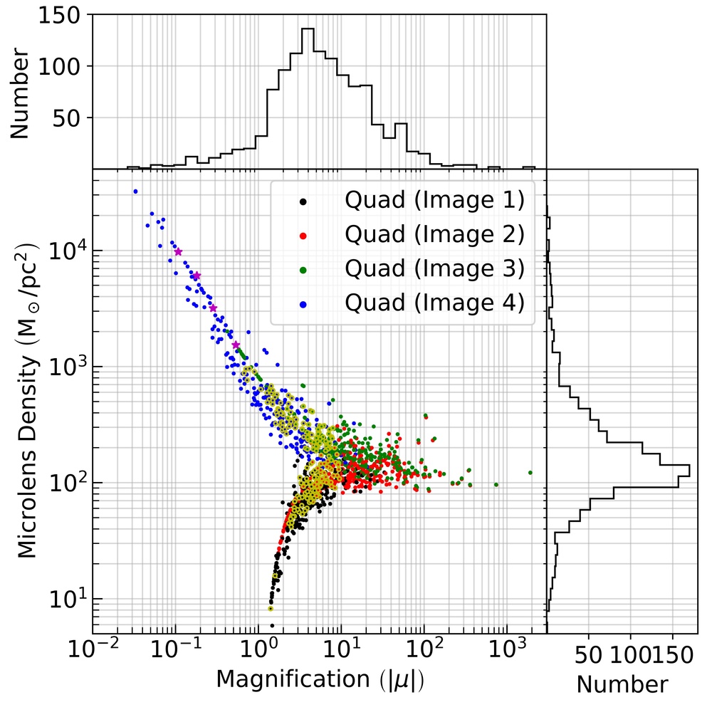
Figure 1: Distribution of images formed in quad lens systems as a function of macro-magnification ($|\mu|$) and microlens density ($\Sigma_{\bullet}$). The black, red, green, and blue points represent the image-1 (minima), image-2 (minima), image-3 (saddle points) and image-4 (saddle points) which are ordered according to their time-delay compared to the global minimum, i.e., image-1. The yellow-edge points represent the 50 lens systems which are analysed in this work whereas the filled maroon stars represent additional 4 cases studied for the saddle points corresponding to image-4 as they are located in regions with extreme microlens densities (${>}10^{3}~{}{\rm M}\odot/{\rm pc^{2}}$) albeit at low magnifications. We also show the 1D histograms of the magnification (top) and microlens density (right) for all four images combined.

2 Simulating lens systems

In this section, we briefly discuss the methodology used to simulate the strong lens systems and the corresponding microlens population for individual strongly lensed images.

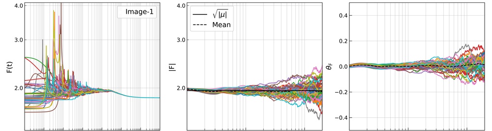
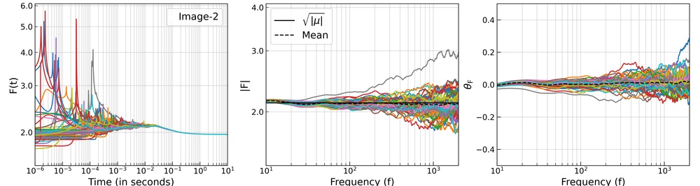
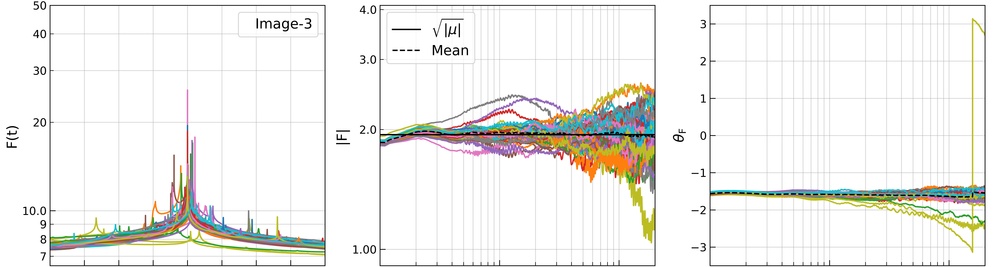
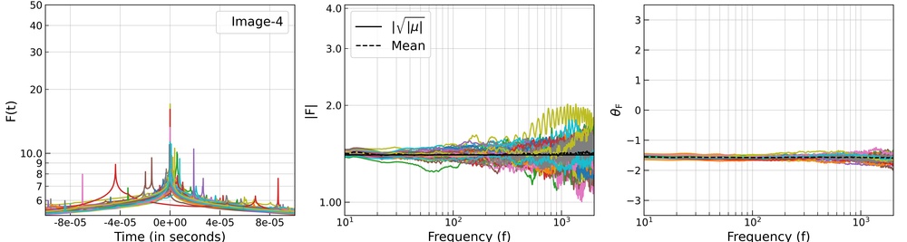
Figure 2: Microlensing effects in all four images (image-1, 2, 3, 4) of one quad lens system. From top-to-bottom, each row corresponds to one of the images in the quad (as indicated by the labels) and each panel shows 50 curves corresponding to the 50 realizations for each image. The left, middle, and right columns represent the $F(t)$, the absolute value of amplification factor ($|F|$), and phase of the amplification factor ($\theta_{\rm F}$). The $F(t)$ curves contain discontinuities and spikes which correspond to micro-minima and micro-saddle points, respectively. In the middle column, the black solid line represents the amplification factor, $\sqrt{|\mu|}$, in the geometric-optics limit which is independent of the frequency. The black dashed curves (in middle and right columns) represent the mean over the 50 realizations.

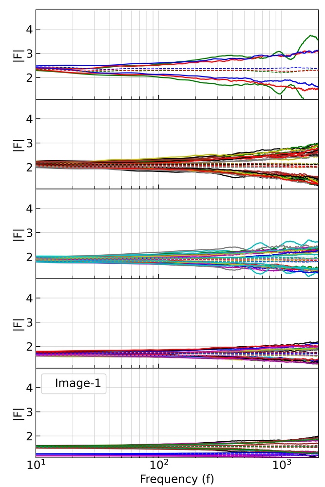
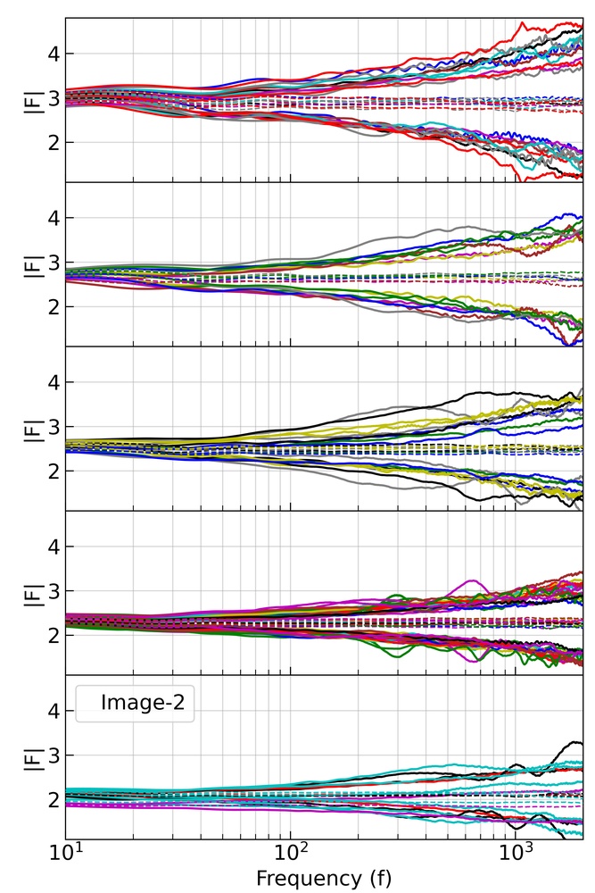
Figure 3: Microlensing effects in minima corresponding to image-1 (left) and image-2 (right). The dotted lines represent the frequency-dependent mean of the absolute amplification factor ($|F|$) based on 50 realizations. The solid lines represent the $3-\sigma$ scatter around the mean. From the bottom-to-top, different lens systems are grouped and split over multiple panels according to their macro-magnifications ($\sqrt{|\mu|}$). Doing so gives improved visual clarity in order to appreciate the magnification-dependence of microlensing effects.

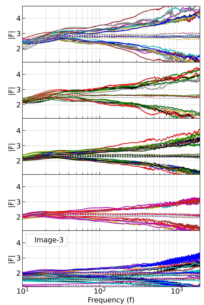
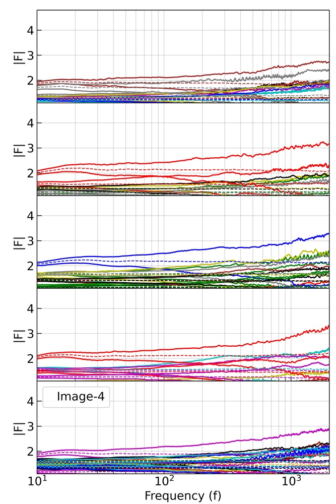
Figure 4: Same as Figure 3 except that the microlensing effects are shown for saddle points corresponding to image-3 (left) and image-4 (right).

2.1 Simulating strongly lensed systems

A strong lens system contains three parts: the source, the lens, and the observer (us). In geometric optics (under thin lens approximation), gravitational lens equation gives a mapping between source plane and lens (image) plane (e.g., Schneider et al., 1992; Narayan & Bartelmann, 1996). As we are mainly focusing here on the lensing of gravitational waves due to a galaxy scale lens in the LIGO frequency range, a typical source will be a merging binary black hole (BBH) system and the lens is assumed to be an elliptical galaxy following a singular isothermal ellipsoid (SIE; Kormann et al., 1994) density profile.

We use the realistically generated mock sample of strong lens systems from More & More (2021, hereafter MM21). We briefly describe below the different assumptions and ingredients of the framework. Assuming that the BBH source is spinless with zero eccentricity, the source population can be described by modeling the three quantities: (i) BBH merger rate, (ii) BBH source redshift, and (iii) BBH component masses. The BBH merger rate has been approximated using the analytical formula given in equation 11 of MM21 (taken from Oguri 2018). Such a functional form roughly reproduce the numerical results shown in Kinugawa et al. (2016) and Belczynski et al. (2017). The source redshift distribution (in the observer frame) depends on the the merger rate and the comoving volume (See equation 12 in MM21). Finally, the BBH component masses are drawn using the power law + peak model given in Abbott et al. (2021).

The lens galaxy population is defined via the: (i) redshift, (ii) velocity dispersion, and (iii) ellipticity (magnitude and a position angle), of the lens. The lens redshift is drawn uniformly in the comoving volume between observer and source. The velocity dispersion is drawn from the modified Schechter function, an observational fit to the Sloan Digital Sky Survey (SDSS) data, following (Choi et al., 2007). The lens ellipticity is drawn from the observed distribution of the elliptical galaxies in the SDSS data (see figure 4 in Padilla & Strauss, 2008).

An SIE lens model gives rise to formation of either two or four image geometry known as doubles and quads (Kormann et al., 1994). In doubles, the pair of images are of different types i.e., a minimum and a saddle point whereas in quads, two of the images are minima and the other two are saddle points. In general, the lensed images are (de-)magnified by different factors and the signal from them takes different amount of time to reach the observer. Typically, the time delay between these lensed images ranges from hours to months for galaxy-scale lenses. The macro-magnification factor corresponding to these different images also depends on the source size: smaller the source, higher the magnification. As mentioned above, since the BBH merger is effectively a point source, the corresponding strongly lensed GW signals can achieve very high magnification (Diego et al., 2019; Mishra et al., 2021). To verify that a GW signal is strongly lensed, we need to observe at least two of the strongly lensed counterparts. Hence, we consider lens systems wherein the second brightest lensed GW signal has a three-detector-network SNR of 8 or above. We note that this detectability criteria is arbitrary and does not affect the conclusions of our work as explained in Section 3. Following the aforementioned procedure, we draw a sample of 300 quads and 200 doubles. This sample contains systems with individual image magnification values up to $10^{3}$. However, as we are mainly focussing on macro-magnification ($|\mu|$) ${\leq}10$ regime we draw a sub-sample of 50 quad systems (randomly) such that all lensed images satisfy $\{|\mu|,\Sigma_{\bullet}\}\leq\{10,10^{3}\>{\rm M}_{\odot}/{\rm pc}^{2}\}$.

2.2 Simulating microlens population

Once we obtain the strong lens systems, the next step is to determine the microlens densities at the position of the strongly lensed images. The microlens density at an image position consists of stars, stellar remnants (white dwarf, neutron star and black hole) and possible compact dark matter objects like primordial black holes (PBH; e.g., Bird et al., 2016; Kovetz, 2017). In this work, we assume that all of the dark matter is in the form of a smooth component leaving only stars and stellar remnants as possible microlenses. To estimate the projected stellar surface mass density at the image positions, we use the Sérsic profile following Vernardos (2019, see equation 8). Since, elliptical galaxies have little to no star formation, only the stars with masses ${\lesssim}1.5{\rm M}_{\odot}$ will contribute to the corresponding projected stellar density as massive stars (${\gtrsim}1.5{\rm M}_{\odot}$) will complete their life in ${\sim}1.5$Gyr. Hence, we draw stellar masses in only the mass range $[0.08,1.5]{\rm M}_{\odot}$ using the Salpeter initial mass function (IMF, Salpeter, 1955). To sample the remnant population, we estimate the corresponding projected surface mass density using the initial-final mass function from the Binary Population And Spectral Synthesis (BPASS; Eldridge et al., 2017). Depending on the IMF and the metallicity, the fraction of remnant mass to the stellar mass can be from ${\sim}5\%$ to ${\sim}20\%$. In our work, we assume this fraction to be $10\%$ at the image positions. As the remnants are dark, we need to add the corresponding surface density to the stellar surface mass density to get final microlens surface mass density. Hence, our final microlens density at an image position is sum of the stellar density and remnant density.

The calculated projected microlens density ($\Sigma_{\rm\bullet}$) for different images and the corresponding macro-magnification for our simulated quads are shown in Figure 1. The black, red, green, and blue points represent the image-1, 2, 3, 4 of the quad systems, respectively. The numbering of the images follows the same order as their arrival times, that is, signal from image-1 is seen first whereas signal from image-4 is seen at the end. Here, we only plot the unsigned magnifications ($|\mu|$) for all of the images leading to a butterfly-shaped distribution in the $|\mu|$–$\Sigma_{\bullet}$ plane. We note that the butterfly shape is not dependent on the detection threshold criteria applied in Section 2.1 As expected the magnification for minima (image-1 and image-2) always have $\mu{\gtrsim}1$ whereas the saddle points in addition can also have $|\mu|{<}1$. Apart from that, the microlens densities for image-1, 2, 3, 4 are in an increasing order. This trend is expected since the saddle points form closer to the center of the lens galaxy in regions of high densities as compared to the minima. In addition, only image-2 and image-3 attains $|\mu|{>}20$ simultaneously as they tend to form in a pair near the critical curve in the lens plane when the source lies near the caustic in the source plane. The 1D histograms of the magnification ($|\mu|$) and the microlens density ($\Sigma_{\bullet}$) are also shown on the panels at the top and to the right, respectively. The magnification peaks below 10 and thus implying most of the individual lensed signals (${\sim}75\%$) in our sample have macro-magnification values below ${\leq}10$. However, in our sample, nearly ${\sim}36\%$ and ${\sim}90\%$ quad and double lens systems, respectively, have their brightest image with macro-magnification ${\leq}10$. On individual image basis in a given sample of quad lens systems, ${\sim}94\%$, ${\sim}36\%$, ${\sim}40\%$, and ${\sim}96\%$ of image-1, image-2, image-3, image-4, respectively, are expected to satisfy the above magnification cut. On the other hand, the microlens density peaks around ${\sim}100~{}{\rm M}_{\odot}/{\rm pc}^{2}$ reflecting the typical microlens densities at the image position in the galaxy-scale lenses. The yellow-edge circles mark the lensed images corresponding to 50 lens systems considered in our analysis. The solid maroon stars show the four images corresponding to image-4 that are chosen to study the high density regions, specifically (see Section 5).

3 Effect of microlens population in strongly lensed systems

To study the effect of microlens population on the strongly lensed GW signal, we need to compute the amplification factor, $F(f)$, which quantifies the wave effects. In the context of GW, it represents the ratio of lensed and unlensed GW waveform in the frequency domain. We consider a patch of $2{\rm pc}\times 2{\rm pc}$ in the lens plane and randomly distribute microlenses in it which are drawn using the procedure discussed in 2.2. Such a patch size ensures that we can go up to a time delay of the order of $0.1$ seconds in the lens plane and, consequently, cover the LIGO frequency range while computing $F(f)$. In the absence of microlensing, there is only one image corresponding to the macro-image forming at the center of the patch. Introducing microlenses divide this macro-image into multiple micro-images. To calculate the $F(f)$, we first calculate its Fourier transform, $F(t)$, in time-domain. The values of $F(t)$ depends on the time delay of different micro-images forming in the patch. In principle, the spread of micro-images in the lens plane depends on the macro-magnification ($|\mu|$) but as we are mainly focussing on $|\mu|<10$ regime, the above patch size is enough. The value of macro-magnification along with the microlens density also determines the underlying computation time: less the macro-magnification or microlens density, less the computation time. We refer readers to Ulmer & Goodman (1995) and Mishra et al. (2021) for more details about the computation method.

Following the above described method, we generate $F(t)$ and $F(f)$ corresponding to all realizations in all 50 lensed systems. In general, the frequency-dependent microlensing effects will be different for different strongly lensed signals as the underlying macro-magnification ($|\mu|$) and microlens densities ($\Sigma_{\bullet}$) vary. However, for a better visualization and understanding of microlensing effects across the different images of a system, we show the microlensing effects for all of the four lensed images of one lens system in Figure 2. The top two rows represent the macro-minima (image-1 and image-2) whereas the bottom two rows represent the macro-saddle points (image-3 and image-4). From left to right, we show the Fourier transform of the amplification factor, $F(t)$, the absolute value of the amplification factor, $|F(f)|$, and the phase of the amplification factor, $\theta_{\rm F}=-\iota\ln\left(F/|F|\right)$, respectively. Each panel shows 50 curves corresponding to the 50 realizations for each image. The $F(t)$ curves start from zero for minima (image-1 and image-2) whereas for the saddle-point, the $F(t)$ curves have non-zero values at negative times. This happens because when a macro-minimum is microlensed, we can always find a global minimum and calculate the time delay of other micro-images with respect to this global minimum (e.g., Saha & Williams, 2011). On the other hand, a macro-saddle point has a global saddle and other micro-images can have both positive and negative time delays with respect to the global saddle. In each $F(t)$ curve, we can see two different kind of features, discontinuities and spikes representing the minima and saddle-point micro-images in the lens plane, respectively. In general, a micro-image forming at a time delay $\delta t$ (compared to the global minimum or global saddle-point) effects $F(f)$ at $f\gtrsim(\delta t)^{-1}$. Therefore, micro-images forming at lower (higher) time-delays lead to slow (rapid) variations in amplification factor, $F(f)$, curve at low frequencies, 10 – 100 Hz.

In the middle column of Figure 2, we show the mean of the 50 realizations (dashed-black curve) and the amplification factor in geometric optics ($\sqrt{|\mu|}$, solid black curve) which is independent of the GW frequency. We find that the mean $|F|$ is close to $\sqrt{|\mu|}$ at all frequencies. The same is also true for the phase in the right column where the mean phase for minima and saddle points remain very close to their geometrical optics values, 0 and $\pi/2$, respectively (Dai & Venumadhav, 2017). This implies that, although for this particular lens system, microlensing introduces additional frequency-dependent fluctuations in the $|F|$ and $\theta_{\rm F}$, these fluctuations are unique to each realization otherwise we would have observed coherent features in the mean value. In addition, the amplitude of these oscillations increases as we go towards higher GW frequencies owing to the multiple faint micro-images forming at higher time-delay values. For image-3, the yellow phase curve, for one of the realizations, shows a discontinuity from $-\pi$ to $\pi$ around 1500 Hz which is an artifact arising from the choice of the limits used to specify the phase.

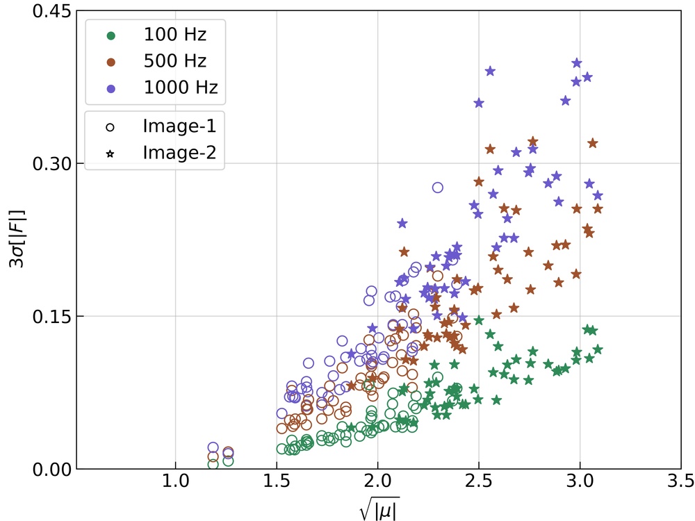
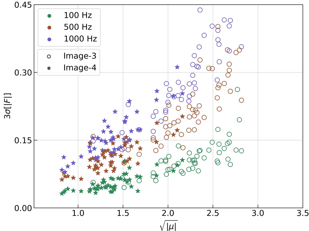
Figure 5: Scatter as a function of the geometric-optics amplification factor ($\sqrt{|\mu|}$) at different GW frequencies, namely, 100 Hz, 500 Hz, and 1000 Hz. The open circles and filled-stars represent image-1 and image-2 in the left panel and image-3 and image-4 in right panel, respectively. At 100 Hz, the $3\sigma$ values increase (roughly) linearly with increasing $\sqrt{|\mu|}$. However, as we increase the frequency (500 Hz and 1000 Hz), the $3\sigma$ values increase more rapidly with $\sqrt{|\mu|}$ and show more scatter compared to 100 Hz implying stronger dependency on the strong lensing amplification factor ($\sqrt{|\mu|}$). See Section 3 for more details.

In Figures 3 and 4, we show the mean and scatter across different realizations for each minimum and saddle point, respectively, from all of the 50 systems. In these figures, the mean $|F|$ (dashed curves) and a ${\pm}3\sigma$ (i.e., ${\pm}3\times$ standard deviation) region around the mean (solid curves) of a given color represent a lens system. In each column, the different lensed images are grouped according to their $\sqrt{|\mu|}$ and plotted in an increasing order from bottom-to-top in different rows for improved clarity. In image-1, 4, we observe that the mean curves do not show significant fluctuations and remain approximately constant in the frequency range [10, 2000] Hz. On the other hand, in image-2, 3 at macro-magnification ${\sim}10$, we begin to see some coherent deviations (compared to the geometric optics value, $\sqrt{|\mu|}$) in the mean curves at low frequencies (${\sim}10$ Hz) implying coherent microlensing-induced fluctuations in all realizations (rise in image-2 and dip in image-3; see Mishra et al., 2021; Diego, 2020). Since these coherent patterns appear near the lower limit of the LIGO frequency band where the detector tends to have decreased sensitivity, it is hard to detect any systematic features in the amplification curves. Nevertheless, with increased sensitivity in the future detectors such as the CE and ET, the probability of identifying such microlensing-induced features, at these frequencies, will increase which may further help us in identifying the lensed nature of the GW event. In addition, we find that as we increase the macro-magnification of the image (from bottom-to-top), the ${\pm}3\sigma$ region becomes relatively wider implying increased amplitude of microlensing fluctuations.

Another interesting observation is that the scatter is affected more by macro-magnification than the underlying microlens density on average. The image-1, with the lowest magnifications, are found in microlens density environments spanning nearly an order of magnitude (see Figure 1). And yet, the mean and the scatter in the amplification curves for those image-1 systems, with very different microlens densities, look barely different from each other (see the bottom-left panel of Figure 3). Any impact on the amplification curves (due to stellar mass microlenses) only become prominent in the presence of high macro-magnification. We note that aforementioned inferences are generally applicable to any minimum or a saddle point. In other words, the trends are similar for all of the images, namely, image-1,2,3 and 4.

To quantify and better depict the dependence of the scatter on the GW frequency and the macro-magnification, in Figure 5, we plot the $3\sigma$ values as a function of strong lensing amplification factor ($|\sqrt{\mu}|$) for all minima (image-1, 2) and saddle points (image-3, 4) in the left and right panels, respectively. As before, the trends are similar for both minima and saddle points, that is, the scatter roughly increases linearly with macro-magnification whereas the slope of this linear curve becomes steeper with increasing frequency.

Although in this work we apply a detection threshold on the second brightest image, our results are valid for any SNR threshold as long as a given lensed image satisfies the criteria applied on the macro-magnification and the microlens density, i.e., $\{|\mu|,\Sigma_{\bullet}\}{\leq}\{10,10^{3}~{}{\rm M}_{\odot}/{\rm pc}^{2}\}$. It is because lowering (raising) the SNR threshold will increase (decrease) the number of detectable lens systems but the corresponding lensed images will still occupy the same region in the $|\mu|-\Sigma_{\bullet}$ plane as shown in Figure 1.

4 (Mis)match Analysis

In this section, we study the magnitude of the microlensing effects on GW signals by calculating the (mis)match between lensed and unlensed GW signal. First, we generate unlensed waveforms using the PyCBC (Usman et al., 2016) with IMRPhenomPv2 approximant and with a lower frequency cut-off ($f_{\rm low}$) at 20 Hz. We further assume that both BBH components are spin-less and the orbit is circular. Next, we produce the lensed waveforms by modifying the unlensed waveforms in the frequency-domain according to a given $F(f)$.

We then calculate the (mis)match as follows. If in the absence of lensing, the GW signal is given by $h_{\rm U}(f)$ in frequency domain then the strongly lensed GW signal will be $h_{\rm SL}(f)=\sqrt{|\mu|}h_{\rm U}(f)$ and strong + microlensed signal will be $h_{\rm ML}(f)=F(f)h_{\rm U}(f)$. The match ($\mathcal{M}$) between lensed, $h_{\rm L}$ (which can be either be $h_{\rm SL}$ or $h_{\rm ML}$), and unlensed waveform ($h_{\rm U}$) is given as (e.g., Usman et al., 2016)

$$\mathcal{M}=\mathop{max}_{t_{0},\phi_{0}}\frac{\langle h_{\rm L}|h_{\rm U}\rangle}{\sqrt{\langle h_{\rm L}|h_{\rm L}\rangle\langle h_{\rm U}|h_{\rm U}\rangle}},$$ (1)

where $t_{0}$ and $\phi_{0}$ are arrival time and phase of $h_{\rm UL}$, respectively. The inner product is noise-weighted and defined as

$$\langle h_{1}|h_{2}\rangle=4{\rm Re}\int_{f_{\rm low}}^{f_{\rm{high}}}df\frac{h_{1}^{*}(f)h_{2}(f)}{S_{n}(f)},$$ (2)

where $S_{n}(f)$ is the single-sided power spectral density of the detector noise. From Equation 1, we can see that the mismatch between unlensed ($h_{\rm U}$) and strongly lensed ($h_{\rm SL}$) waveform will be zero as strong lensing only (de)amplifies the unlensed waveform by a constant factor, $\sqrt{|\mu|}$. Hence, the mismatch between $h_{\rm U}$ and $h_{\rm ML}$ will only arise due to features introduced by microlensing. A high match ($\mathcal{M}>99\%$) generally implies that any deviations due to microlensing are weak and will go undistinguished (e.g., Cao et al., 2014). We note that the above mentioned match is between lensed and unlensed waveform and not the maximum match ($\mathcal{M}_{\rm max}$) which represents the maximum match against a template bank. In general, the $\mathcal{M}_{\rm max}$ is expected to be larger than $\mathcal{M}$.

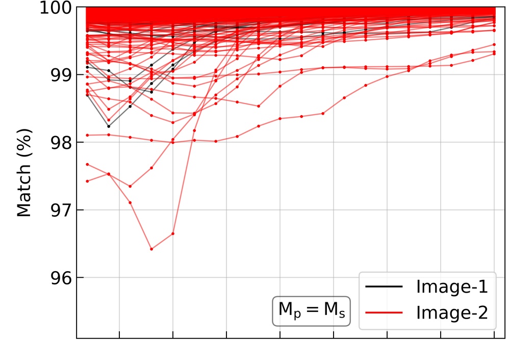
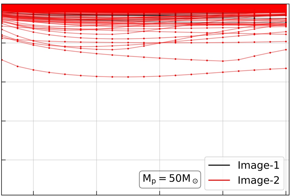
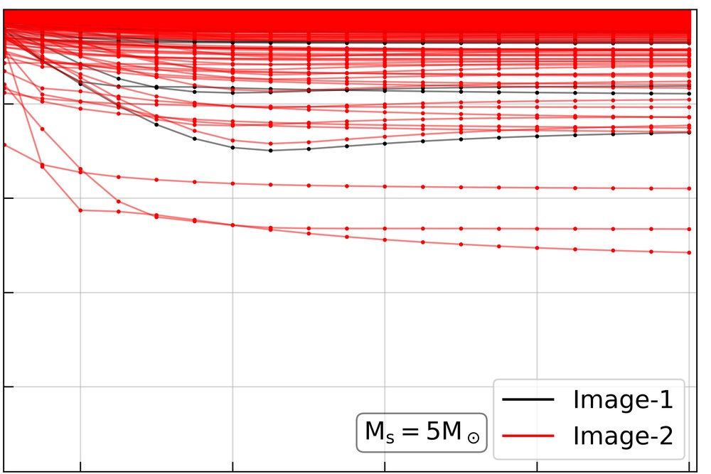
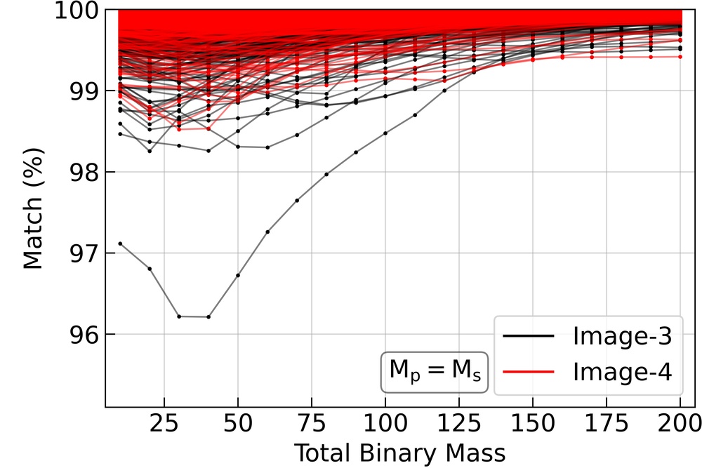
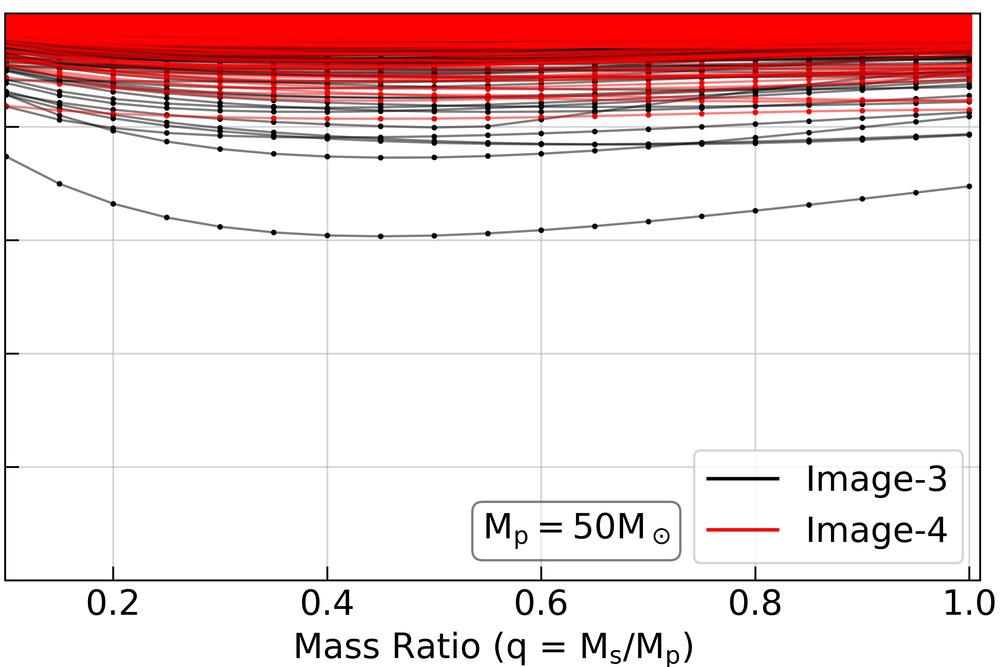
Figure 6: Match between unlensed and lensed GW signals as a function of the BBH total mass (left column) and the mass ratio (middle and right columns). The upper and lower rows show results for image-1, 2 and image-3, 4, respectively. For each image, results are shown for 2500 microlensed signals (50 quads $\times$ 50 realizations). Assuming equal masses for the primary ($M_{\rm p}$) and the secondary ($M_{\rm s}$) components of a BBH (left column), the mismatch is found to be worse for low-mass BBHs compared to higher mass BBHs. For a fixed mass of $M_{\rm p}=50~{}{\rm M}_{\odot}$ for the primary (middle column), we find that the match does not vary significantly as a function of the mass ratio of the BBH although it is marginally better for systems with extreme mass ratios. Similar trends are seen when varying the mass ratio while the secondary is fixed to $M_{\rm s}=5~{}{\rm M}_{\odot}$ (right column).

In Figure 6, we show the match for all of the images from a quad (top row for image-1, 2 and bottom row for 3, 4). As we have 50 quad systems and for each image, we simulate 50 realizations, each panel contains a total of 2500 curves corresponding to each image. In the left panel, we vary the BBH total masses assuming both components have equal mass, i.e., $M_{\rm p}=M_{\rm s}$, where $M_{\rm p}$ and $M_{\rm s}$ are primary and secondary component masses. In the middle (right) panel, we vary the mass ratios while fixing the primary (secondary) component mass to $50\>(5)\>{\rm M}_{\odot}$. The general conclusion from Figure 6 is that the match is always greater than 99% for most of the realizations and only a handful (${<}1\%$) of realizations shows match less than 99%. This implies that the GW detection pipelines are unlikely to miss any GW signals that are affected by microlensing. Hence, we do not expect any significant bias in the estimated values of the BBH parameters. We note that $\mathcal{M}_{\rm max}<97\%$ is a detection threshold typically used by GW detection pipelines rather than a threshold of $\mathcal{M}<99\%$ and, as mentioned above, $\mathcal{M}_{\rm max}$ is expected to be larger than $\mathcal{M}$. Hence, $\mathcal{M}~{}{\sim}~{}99\%$ is anticipated to lead $\mathcal{M}_{\rm max}\gtrsim 99\%$.

Additionally, in Figure 6, the match value increases as we increase the mass of the binary components. This is because massive binaries mainly emit GWs at low frequencies and the amplitude of the microlensing effects is weak at such low frequencies although it gets stronger with increasing frequency. Apart from this, in general, we also observe that image-1 shows a higher match compared to other images. This can be understood from the fact image-1 is the global minimum with low-to-moderate macro-magnification and it forms in relatively low microlens density regions compared to other images. On the other hand, image-4, which is closest to the lens center, in general, gets de-magnified leading to match values similar to image-1. As expected, image-2 and image-3 tend to have higher mis-match (i.e. $\mathcal{M}<99\%$) more often than image-1 and image-4.

The above observations imply that if the macro-magnification is $\leq 10$ then the probability of mismatch between lensed and unlensed signal being worse than 1% is less than 0.01. This probability further decreases for image-1 and (nearly) always remains unwavered across multiple realisations of the microlens population. Hence, as a first order approximation, we can safely assume negligible microlensing effects from stellar mass microlenses in strongly lensed GW signals with $|\mu|\leq 10$, especially, for image-1. The advantage here is that, among a pair or triplet, identified as a candidate lens system, if we can detect the image-1 then it can be used as a reference GW signal to estimate the microlensing effects in other lensed counterparts. In Seo et al. (2021), a similar idea is explored to show improvement in the parameter estimation of a single microlens. However, to study the microlensing effects due to a microlens population in a strongly lensed GW candidate, creating many realizations of the microlens population will probably become imperative.

Although less probable, in rare cases, microlensing due to stellar mass objects can lead to notable effects even in the $|\mu|\leq 10$ regime (see Figure 6). This can happen (not always though) if one or a few microlenses lie around an Einstein-radius distance from the patch center in the lens plane. We find that, all realizations leading to low match (${<}98\%$) in Figure 6, have a massive microlens with mass ${\sim}20\>{\rm M}_{\odot}$ located around 1–5 Einstein radius (of the microlens) away from the patch center. Hence, our results imply that, in general, microlensing due to stellar-mass microlenses at low macro-magnification leads to negligible mismatch (e.g., Cheung et al., 2021), however, presence of microlenses near the patch center may lead to significant mismatch even if the macro-magnification is small.

We determine the probability of seeing a match below the threshold of 99% as a function of the macro-magnification and the BBH properties, for example, the total BBH mass and the mass ratio. We calculate these probabilities for all image-1,2,3,4 but choose to show the results only for image-2 and image-3 in Figure 7 where the mismatch is a bit more significant than image-1 and image-4. We find that larger fractions of images show a high mismatch at low-mass BBHs (left column), particularly, at high macro-magnifications. We do not see significant dependency on the BBH mass ratio for the fraction of images (see right column and Figure 6). We find that macro-magnification plays the most important role. The trends are similar in both image-2 and image-3.

Figure 7: Fraction of images with match ${<}99\%$ ($f_{\mathcal{M}}$) as a function of the macro-magnification (y-axes) and the total binary mass (x-axis) for the column on the left and as a function of the mass ratio (x-axis) for the column on the right. The top and bottom rows are for image-2 and image-3, respectively. Mismatch is higher for higher macro-magnifications and for low-mass binaries.

5 High Microlens Density

So far our analysis was focused on strongly lensed systems with $\{|\mu|,\Sigma_{\bullet}\}\leq\{10,~{}10^{3}~{}{\rm M}_{\odot}/{\rm pc}^{2}\}$. However, we can see from Figure 1 that this does not cover the allowed $|\mu|-\Sigma_{\bullet}$ parameter space completely. The image-2 and image-3 image-pair can attain very high macro-magnifications ($|\mu|{>}100$) for a BBH source located near the caustic in the source plane due to its point source nature. On the other hand, image-4 can form in the lens plane where the microlens densities can go above $10^{3}~{}{\rm M}_{\odot}/{\rm pc}^{2}$. In this section, we study the microlensing effects in image-4 with $\Sigma_{\bullet}>10^{3}~{}{\rm M}_{\odot}/{\rm pc}^{2}$. We select four individual image-4 images (see maroon stars in Figure 1) with microlens densities in the range $(10^{3},10^{4})~{}{\rm M}_{\odot}/{\rm pc}^{2}$. The corresponding macro-magnifications ($|\mu|$) lie in the range (0.1, 0.6). For each of the four images, we again simulate 50 realizations with a patch-size of 2 pc $\times$ 2 pc.

The resulting absolute amplification ($|F|$) curves as a function of GW frequencies are shown in Figure 8. For all four cases, we see two different kind of features: (i) random oscillations unique to each realization with increasing amplitude as we go from low to high frequencies. (ii) coherent oscillations across all realizations of image with $\Sigma_{\bullet}{=}9927~{}{\rm M}_{\odot}/{\rm pc}^{2}$ at low frequencies (${\sim}20$ Hz). The random oscillations are genuine features arising due to the presence of microlens population and unique in each realizations as the microlenses are randomly distributed. The coherent oscillations, at low frequencies, are artifacts and are arising due to the finite patch size. It turns out that a small patch can lead to the formation of spurious micro-images at large time delays which leads to frequency-dependent oscillations at low frequencies. If we simulate a bigger patch, these oscillations will disappear. But, simulating a large patch implies an increase in the number of microlenses leading to increase in the computational times. Apart from that, the $|F|$ curves only show variation of $\sim 0.2-0.3$ over the mean magnification which tends to be less than one and thus, the amplitude of these oscillations is not significant across LIGO–Virgo frequencies (10 Hz to $10^{3}$ Hz) resulting in negligible effects in the mismatch as well as the parameter estimation. Considering these factors, we choose not to simulate bigger patches in the lens plane as it is expected to not affect our conclusion. We conclude that the microlensing-driven frequency-dependent effects (due to stellar mass population) are negligible in de-magnified lensed GW signals located in high microlens density regions within the lens galaxy.

6 Two image systems (Doubles)

Until now, we have been investigating quads but since the SIE lens models produce both doubles and quads which is also consistent with real observations of lens samples, we briefly discuss implications of our results on images belonging to doubles. Fortunately, the image-1, 2 of doubles have a significant overlap with the images in quads in the $|\mu|-\Sigma_{\bullet}$ plane. We verify this by over-plotting 200 doubles generated in a similar way to the quads in the $|\mu|-\Sigma_{\bullet}$ plane as shown in Figure 9. Note that the underlying quad population is the same as shown in Figure 1 except that all four images (image-1, 2, 3, 4) from a quad are shown by a single black color for reference and as before, the yellow edge circles highlight the 50 systems used in our analysis. The red and green points now show the image-1, 2 corresponding to minima and saddle points found in doubles.

This extensive overlap implies that the minima and saddle points formed in the doubles and quads are found in similar lens environments, that is, similar combinations of macro-magnifications and microlens densities leading to a similar butterfly-like distribution in the $|\mu|$–$\Sigma_{\bullet}$ plane. It is then safe to use the minima and saddle point realizations from the sample of quads to deduce the microlensing effects expected to be seen in a sample of doubles. As a result, our conclusions inferred from the images belonging to quads are also applicable to images belonging to doubles.

This is an important result to be noted because from an observational point of view, there tends to be an ambiguity whether a pair of candidate lensed events belong to a double or a quad. Only when the image types of the pair are robustly known and are expected to have the same type (i.e., they both are either minima or saddle points) can we be certain that the pair of images are from a quad. However, since the degree of microlensing effects are similar for both doubles and quads, it is not required to know beforehand the image types or the true multiplicity of a lens system (i.e. a double or a quad).

We see that in our sample of doubles, only a couple of lens systems have saddle points with microlens densities ${>}10^{3}~{}{\rm M}_{\odot}$. This is because increasing density will decrease the strong lens magnification which leads the SNR to drop below 8. However, as discussed in Section 5, the amplitude of microlensing effects further decreases. This only depends on the strong lensing information, hence, the results from Section 5 can again be extrapolated for double image systems.

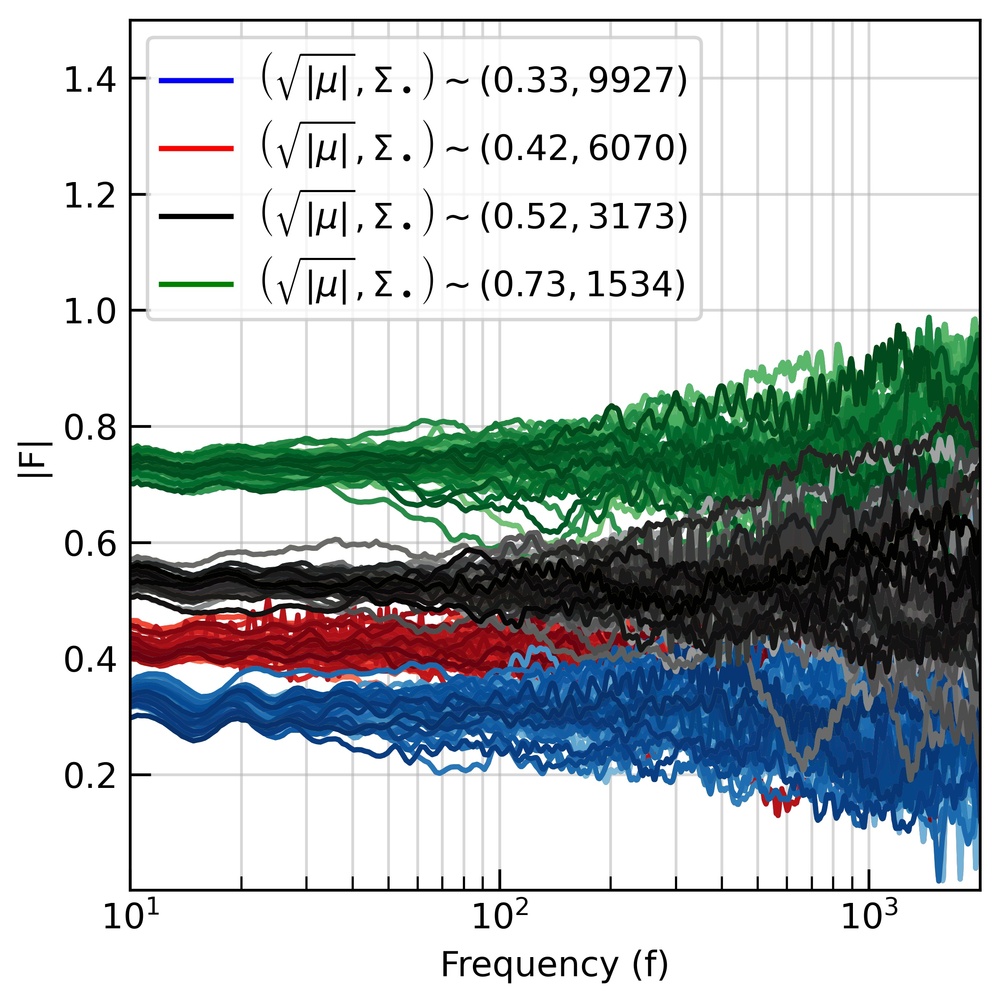
Figure 8: Microlensing effects seen in the saddle points of image-4 in high density regions. The amplification factor ($|F|$) is shown as a function of frequency for four different combinations of $\{|\mu|,\>\Sigma_{\bullet}\}$ (corresponding to maroon stars in Figure 1). There are 50 realizations for each of the four cases and their respective macro-magnifications and microlens densities are given in the legend. The amplitude of the distortions due to microlensing is negligible despite the high microlens densities owing to the low macro-magnification of these images. See Section 5 for more details.

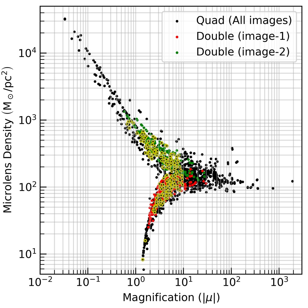
Figure 9: Distributions of doubly lensed images in the plane of macro-magnification ($|\mu|$) and microlens density ($\Sigma_{\bullet}$) as compared to the distributions seen in the lensed images of quads. The black dots represent all four images (image-1, 2, 3, 4) of the simulated quads (same as the quads in Figure 1). The red and green points represent the minima (image-1) and saddle points (image-2) belonging to doubles, respectively. The yellow-edge points denote the 50 quads used in our analysis. The overlap between quads and doubles in this plane implies the minima and saddle points of doubles have similar local environments and thus, results obtained for quads hold true for doubles.

7 Discussion and Conclusions

The goal of this work is to study realistic samples of galaxy-scale lens systems in order to assess the probability of microlensing arising due to realistic stellar populations and to understand the extent to which microlensing could affect the detectability of strongly lensed GW events. We investigated the effect of microlensing on two types of lensed images, minima and saddle points, found in typical galaxy-scale lenses where the images have low-to-moderate macro-magnifications ($|\mu|=(0.5,10)$) and are located in typical microlens density environments $(\Sigma_{\bullet}=(10,10^{3})~{}{\rm M}_{\odot}/{\rm pc}^{2})$ in the LIGO frequency band ($10$ Hz – $10^{4}$ Hz).

In our earlier work Mishra et al. (2021), we studied the microlensing effects for individual minima and saddle points considering specific macro-magnification and microlens density values appropriate for galaxy lenses, however, the underlying goal was to identify which parameters influence microlensing the most and how severe the microlensing effects could be for those specific scenarios. In the current work, we are studying the lens population as a whole to determine the fraction of galaxy-scale lenses that could be affected by microlensing and to what extent. To do so, we considered a total of 50 quadruply-imaged lens systems (quads) where the second brightest image has a three-detector network-SNR greater than 8 (corresponding to the LIGO-O3 sensitivity). For each strongly lensed image within a quad, we generated 50 realizations to study the scatter (introduced due to microlensing) in the amplification factor. We also calculated the mismatch between the lensed and unlensed GW signals to understand how microlensing will distort and modulate the individual lensed signal and different lensed GW counterparts of a signal. Furthermore, the image-4, which forms near the lens center, tends to be located in high microlens density regions ($\Sigma_{\bullet}{>}10^{3}~{}{\rm M}_{\odot}/{\rm pc}^{2}$). Since understanding the microlensing effects in such extreme conditions is also important but computationally expensive, we considered only four high microlens density cases by generating 50 realizations for each case, as done earlier. In addition to the quads, we also expect to find doubly imaged lenses (doubles) among the galaxy-scale lens systems. Even though we only studied images belonging to quads in this work, we discussed their similarity with the images in doubles and validity of our results for doubles.

The main conclusions of our work are described below.

• We find that the microlensing effects are more sensitive to the macro-magnification than the underlying microlens density (constituting stellar mass objects) similar to Mishra et al. (2021). Even when the images are located in extremely high microlens density regions ($>10^{3}~{}{\rm M}_{\odot}/{\rm pc}^{2}$), the microlensing distortions are minimal due to low macro-magnification.

• For both minima and saddle points with macro-magnification ${\leq}~{}10$, the microlensing due to stellar-mass objects does introduce frequency-dependent effects. However, in ${>}~{}99\%$ cases, the mismatch (between lensed and unlensed GW signals) remains ${<}~{}1\%$ as the amplitude of microlensing distortions is not significant enough. Thus, the detectability of any of the strongly lensed images with $|\mu|\leq 10$ is unlikely to be affected by microlensing due to stellar mass objects (Cheung et al., 2021). This also implies that at $|\mu|\leq 10$ we expect negligible bias due to microlensing in parameter estimation and identification of different lensed counterparts alleviating the concern highlighted in Meena & Bagla (2020).

• The strongly lensed GW signal corresponding to global minima (image-1) is the least affected by microlensing for all total masses and mass ratios of the BBH. Hence, if any of the remaining lensed images are identified together with image-1, we can use the image-1 as an uncontaminated “reference" image to estimate unambiguously the microlensing-specific effects on the other lensed images and hence, potentially, their microlensing model parameters too.

• For a given strongly lensed signal, the microlensing distortions increase with increasing the GW frequency (as also noted in Mishra et al. 2021). Hence, a low-mass BBH, wherein the binary coalesce at higher frequencies, is expected to show more significant microlensing effects compared to a high-mass BBH.

• In general, since the image-4 is de-magnified, it will tend to be below the threshold of standard GW detection pipelines (i.e. a sub-threshold event). A magnification boost from microlensing could make such events to become super-threshold, in principle. However, this is almost impossible in reality (considering the stellar mass population) as the amplitude of the microlensing distortions are weak for all of the $|\mu|\leq 10$ image-4 explored in our analysis. Further de-magnification from microlensing will likely make it even more difficult to find image-4, generally.

• Our conclusions are equally valid for doubles, since their minima and saddle points occupy the same region in the macro-magnification vs microlens density ($|\mu|-\Sigma_{\bullet}$) plane, as long as the $|\mu|\leq 10$.

• We note that ${\sim}40\%$ of detectable event pairs from quads and and ${\sim}90\%$ of the doubles from our realistic mocks, corresponding to current LIGO–Virgo sensitivities, meet the $|\mu|\leq 10$ cut. For the fourth observing run of LIGO–Virgo, the fractions become ${\sim}50\%$ for quads and remain nearly the same for the doubles. But with future detectors such as the Cosmic Explorer or Einstein Telescope, these fractions rise up to ${\sim}90\%$ and ${\sim}99\%$ for quads and doubles, respectively.

Our conclusions have implications in the detection of strongly lensed GW event pairs. Searching methods such as ranking statistic to identify strongly lensed candidate pairs, for example, ${\cal M}^{\rm gal}$ (MM21) are based on joint distributions of magnifications and time-delays. They rely on the fact that there are correlations between the relative magnifications and time-delays of a pair of strongly lensed signals. If microlensing causes significant distortions to magnifications of one or both of the lensed signals, then the ranking statistic based on joint distributions could fail to identify a strongly lensed event pair correctly. However, our analysis suggests that the relative magnifications will be unaffected by microlensing for almost all lensed signals with $|\mu|\leq 10$ and thus, offering a fast and robust means of identifying candidate lensed event pairs.

As mentioned earlier, the global minimum (image-1) for $|\mu|{\leq}10$ does not get significantly affected by the microlensing due to stellar mass microlenses. However, high-mass microlenses (${>}100~{}{\rm M}_{\odot}$) may still lead to detectable frequency-dependent modulations. The detection of such high-mass BBH sources in LIGO (The LIGO Scientific Collaboration et al., 2021) implies that such objects are present in galaxies albeit in small numbers probably. Hence, image-1, if affected by high-mass microlenses, may become an excellent probe to study this microlens population in lens galaxies (as the stellar mass microlenses lead to negligible microlensing-effects) and may allow us to put constraint on their properties. We plan to investigation this in our future work.

It is very likely that our results will not be applicable for lensed signals with macro-magnification ($|\mu|$) ${>}~{}10$. In general, we expect that image-2 and image-3 pair to attain very high magnification whereas the corresponding image-1 and image-4 to have low-to-moderate macro-magnification. In such cases, the estimated parameters values for image-2, 3 pair can be significantly different than image-1, 4 (Meena & Bagla, 2020). Hence, we will study the microlensing effects in systems where one or more lensed counterparts has macro-magnification $(|\mu|)>10$ in a subsequent paper.

8 Acknowledgements

AKM would like to thank the Ministry of Science and Technology, Israel for financial support. A. Mishra would like to thank the University Grants Commission (UGC), India, for financial support as a research fellow. Authors gratefully acknowledge the use of high performance computing facilities at IUCAA, Pune. This research has made use of NASA’s Astrophysics Data System Bibliographic Services.

9 Data Availability

The simulated strong lens system data is available from MM21 upon reasonable request. The microlensing simulation data can be made available upon reasonable request to the corresponding author.

References

- Abbott et al. (2018) Abbott B. P., et al., 2018, Living Reviews in Relativity, 21, 3
- Abbott et al. (2021) Abbott R., et al., 2021, Physical Review X, 11, 021053
- Acernese et al. (2015) Acernese F., et al., 2015, Classical and Quantum Gravity, 32, 024001
- Akutsu et al. (2021) Akutsu T., et al., 2021, Progress of Theoretical and Experimental Physics, 2021, 05A101
- Bailes et al. (2021) Bailes M., et al., 2021, Nature Reviews Physics, 3, 344
- Baraldo et al. (1999) Baraldo C., Hosoya A., Nakamura T. T., 1999, Phys. Rev. D, 59, 083001
- Barausse et al. (2020) Barausse E., et al., 2020, General Relativity and Gravitation, 52, 81
- Belczynski et al. (2017) Belczynski K., Ryu T., Perna R., Berti E., Tanaka T. L., Bulik T., 2017, MNRAS, 471, 4702
- Bird et al. (2016) Bird S., Cholis I., Muñoz J. B., Ali-Haïmoud Y., Kamionkowski M., Kovetz E. D., Raccanelli A., Riess A. G., 2016, Phys. Rev. Lett., 116, 201301
- Bontz & Haugan (1981) Bontz R. J., Haugan M. P., 1981, Ap&SS, 78, 199
- Broadhurst et al. (2018) Broadhurst T., Diego J. M., Smoot George I., 2018, arXiv e-prints, p. arXiv:1802.05273
- Bulashenko & Ubach (2021) Bulashenko O., Ubach H., 2021, arXiv e-prints, p. arXiv:2112.10773
- Cao et al. (2014) Cao Z., Li L.-F., Wang Y., 2014, Phys. Rev. D, 90, 062003
- Cheung et al. (2021) Cheung M. H. Y., Gais J., Hannuksela O. A., Li T. G. F., 2021, MNRAS, 503, 3326
- Choi et al. (2007) Choi Y.-Y., Park C., Vogeley M. S., 2007, ApJ, 658, 884
- Christian et al. (2018) Christian P., Vitale S., Loeb A., 2018, Phys. Rev. D, 98, 103022
- Dai & Venumadhav (2017) Dai L., Venumadhav T., 2017, arXiv e-prints, p. arXiv:1702.04724
- Dai et al. (2020) Dai L., Zackay B., Venumadhav T., Roulet J., Zaldarriaga M., 2020, arXiv e-prints, p. arXiv:2007.12709
- Deguchi & Watson (1986) Deguchi S., Watson W. D., 1986, Phys. Rev. D, 34, 1708
- Diego (2019) Diego J. M., 2019, A&A, 625, A84
- Diego (2020) Diego J. M., 2020, Phys. Rev. D, 101, 123512
- Diego et al. (2019) Diego J. M., Hannuksela O. A., Kelly P. L., Pagano G., Broadhurst T., Kim K., Li T. G. F., Smoot G. F., 2019, A&A, 627, A130
- Eldridge et al. (2017) Eldridge J. J., Stanway E. R., Xiao L., McClelland L. A. S., Taylor G., Ng M., Greis S. M. L., Bray J. C., 2017, Publ. Astron. Soc. Australia, 34, e058
- Evans et al. (2021) Evans M., et al., 2021, arXiv e-prints, p. arXiv:2109.09882
- Janquart et al. (2021) Janquart J., Seo E., Hannuksela O. A., Li T. G. F., Broeck C. V. D., 2021, The Astrophysical Journal Letters, 923, L1
- Kawamura et al. (2021) Kawamura S., et al., 2021, Progress of Theoretical and Experimental Physics, 2021, 05A105
- Kinugawa et al. (2016) Kinugawa T., Miyamoto A., Kanda N., Nakamura T., 2016, MNRAS, 456, 1093
- Kormann et al. (1994) Kormann R., Schneider P., Bartelmann M., 1994, A&A, 284, 285
- Kovetz (2017) Kovetz E. D., 2017, Phys. Rev. Lett., 119, 131301
- LIGO Scientific Collaboration et al. (2015) LIGO Scientific Collaboration et al., 2015, Classical and Quantum Gravity, 32, 074001
- Lai et al. (2018) Lai K.-H., Hannuksela O. A., Herrera-Martín A., Diego J. M., Broadhurst T., Li T. G. F., 2018, Phys. Rev. D, 98, 083005
- Lawrence (1971) Lawrence J. K., 1971, Nuovo Cimento B Serie, 6B, 225
- Li et al. (2019) Li A. K. Y., Lo R. K. L., Sachdev S., Chan C. L., Lin E. T., Li T. G. F., Weinstein A. J., 2019, arXiv e-prints, p. arXiv:1904.06020
- Lo & Magana Hernandez (2021) Lo R. K. L., Magana Hernandez I., 2021, arXiv e-prints, p. arXiv:2104.09339
- Maggiore et al. (2020) Maggiore M., et al., 2020, J. Cosmology Astropart. Phys., 2020, 050
- McIsaac et al. (2020) McIsaac C., Keitel D., Collett T., Harry I., Mozzon S., Edy O., Bacon D., 2020, Phys. Rev. D, 102, 084031
- Meena & Bagla (2020) Meena A. K., Bagla J. S., 2020, MNRAS, 492, 1127
- Mishra et al. (2021) Mishra A., Meena A. K., More A., Bose S., Bagla J. S., 2021, MNRAS, 508, 4869
- More & More (2021) More A., More S., 2021, arXiv e-prints, p. arXiv:2111.03091
- Nakamura (1998) Nakamura T. T., 1998, Phys. Rev. Lett., 80, 1138
- Nakamura & Deguchi (1999) Nakamura T. T., Deguchi S., 1999, Progress of Theoretical Physics Supplement, 133, 137
- Narayan & Bartelmann (1996) Narayan R., Bartelmann M., 1996, arXiv e-prints, pp astro–ph/9606001
- Oguri (2018) Oguri M., 2018, MNRAS, 480, 3842
- Ohanian (1974) Ohanian H. C., 1974, International Journal of Theoretical Physics, 9, 425
- Padilla & Strauss (2008) Padilla N. D., Strauss M. A., 2008, MNRAS, 388, 1321
- Saha & Williams (2011) Saha P., Williams L. L. R., 2011, MNRAS, 411, 1671
- Salpeter (1955) Salpeter E. E., 1955, ApJ, 121, 161
- Schneider et al. (1992) Schneider P., Ehlers J., Falco E. E., 1992, Gravitational Lenses, doi:10.1007/978-3-662-03758-4.
- Seo et al. (2021) Seo E., Hannuksela O. A., Li T. G. F., 2021, arXiv e-prints, p. arXiv:2110.03308
- Takahashi & Nakamura (2003) Takahashi R., Nakamura T., 2003, ApJ, 595, 1039
- The LIGO Scientific Collaboration et al. (2021) The LIGO Scientific Collaboration et al., 2021, arXiv e-prints, p. arXiv:2111.03606
- Ulmer & Goodman (1995) Ulmer A., Goodman J., 1995, ApJ, 442, 67
- Usman et al. (2016) Usman S. A., et al., 2016, Classical and Quantum Gravity, 33, 215004
- Vernardos (2019) Vernardos G., 2019, MNRAS, 483, 5583
- Vijaykumar et al. (2022) Vijaykumar A., Mehta A. K., Ganguly A., 2022, arXiv e-prints, p. arXiv:2202.06334