Rates and Properties of Strongly Gravitationally Lensed Supernovae
and their Host Galaxies in Time-Domain Imaging Surveys
Abstract
Supernovae that are strongly gravitationally lensed (gLSNe) by galaxies are powerful probes of astrophysics and cosmology that will be discovered systematically by wide-field, high-cadence imaging surveys such as the Zwicky Transient Facility (ZTF) and the Large Synoptic Survey Telescope (LSST). Here we use pixel-level simulations that include observing strategy, target selection, supernova properties, and dust to forecast the rates and properties of gLSNe that ZTF and LSST will find. Applying the resolution-insensitive discovery strategy of Goldstein et al. (2018), we forecast that ZTF (LSST) can discover 0.02 (0.79) 91bg-like, 0.17 (5.92) 91T-like, 1.22 (47.84) Type Ia, 2.76 (88.51) Type IIP, 0.31 (12.78) Type IIL, and 0.36 (15.43) Type Ib/c gLSNe per year. We also forecast that the surveys can discover at least 3.75 (209.32) Type IIn gLSNe per year, for a total of at least 8.60 (380.60) gLSNe per year under fiducial observing strategies. ZTF gLSNe have a median , , , days, , and . LSST gLSNe are less compact and less magnified, with a median , , , days, , and . We develop a model of the supernova–host galaxy connection and find that the vast majority of gLSN host galaxies will be multiply imaged, enabling detailed constraints on lens models with sufficiently deep high-resolution imaging taken after the supernova has faded. We release the results of our simulations as catalogs at http://portal.nersc.gov/project/astro250/glsne/.
1 Introduction
When a supernova explodes far behind a foreground galaxy, the galaxy’s strong gravitational field can create multiple images of the supernova in different places on the sky (Einstein, 1936; Zwicky, 1937). Because these images travel along different geometric paths and through different gravitational potentials to reach us, they arrive at different times, and in general they can be highly magnified (Refsdal, 1964a). Time delays between the multiple images of these “strongly gravitationally lensed supernovae” (gLSNe) can be used to measure the Hubble constant H0 (Refsdal, 1964b), which is currently in tension at the level (Riess et al., 2018), independently of the local distance ladder and the assumed cosmological model (e.g., Birrer et al., 2018). If a gLSN is discovered before all of its images arrive, early moments of the supernova can be observed by anticipating the appearance of the remaining images (e.g., Goldstein et al., 2018; Suwa, 2018). These remarkable attributes make gLSNe valuable probes of astrophysics and cosmology.
To date, only two gLSNe with resolved images have been discovered (Kelly et al., 2015a; Goobar et al., 2017). Neither has yielded competitive constraints on H0 (but see Suyu et al., 2017; Bonvin et al., 2017; Grillo et al., 2018; Vega-Ferrero et al., 2018), nor observations of the earliest moments of the supernova light curve. However, a new generation of high-cadence, wide-field imaging surveys, exemplified by the Zwicky Transient Facility (ZTF; 2018–2021; Graham et al., in preparation), the Large Synoptic Survey Telescope (LSST; 2021–2033; LSST Science Collaboration et al. 2009), and the Wide-Field Infrared Survey Telescope (WFIRST; 2025–2031; Spergel et al. 2013) is expected to yield thousands of gLSNe over the next decade (Goldstein & Nugent 2017; Goldstein et al. 2018, see also Oguri & Marshall 2010). These surveys will cover enough of the sky, to sufficient depth, at a high enough cadence to produce the first statistical samples of gLSNe. They will also be the first to employ novel detection techniques that will eliminate the need to resolve multiple images for gLSN discovery, furthering the yield. Finally, they will implement highly tuned gLSN filters that will lead to early discovery and minimization of false positives.
To calibrate scientific expectations for the gLSN era, reliable forecasts of gLSN yields and properties are needed. Schneider & Wagoner (1987) and Linder et al. (1988) carried out the first gLSN property forecasts, and Kolatt & Bartelmann (1998), Sullivan et al. (2000), Holz (2001), Dobler & Keeton (2006), Oguri & Marshall (2010), Goldstein & Nugent (2017), Goldstein et al. (2018), and Shu et al. (2018) presented refined calculations. Each of these studies neglected to account for at least one of the following important effects: observing strategy and conditions, dust, discovery strategy, multiple supernova subtypes and rates, and the supernova-host galaxy connection. In anticipation of the gLSN era, we present the first pixel-level Monte Carlo, ray-tracing, and image simulations of the gLSN population to include a detailed treatment of these important effects and use them to forecast gLSN rates and properties. In Section 2, we describe our models of the supernova, host galaxy, deflector, and lens galaxy populations. In Section 3, we present the results of our simulations, including gLSN yields and time delay, brightness, and image separation distributions. We discuss the implications of our results in Section 4 and conclude in Section 5. In our calculations we assume a Planck Collaboration et al. (2016) cosmology.
2 Population Models
In this section, we describe the models of the deflector, lens galaxy, supernova, and host galaxy populations that we use to forecast the rates and properties of gLSNe from upcoming surveys.
2.1 Deflectors
Although galaxy clusters and late-type galaxies can act as gravitational lenses for background supernovae, we consider only elliptical galaxies as lenses in this analysis. We model the projected mass distribution of elliptical galaxies as a Singular Isothermal Ellipsoid (SIE; Kormann et al., 1994), which has shown excellent agreement with observations (e.g., Koopmans et al., 2009). The SIE convergence is given by:
| (1) |
where
| (2) |
In the above equations, is the velocity dispersion of the lens galaxy, is its ellipticity, and is its so-called “dynamical normalization,” a parameter related to three-dimensional shape, and and are the angular diameter distances between the lens and the source and the observer and the source, respectively. Here we make the simplifying assumption that there are an equal number of oblate and prolate galaxies, which Chae (2003) showed implies . We model the velocity distribution of elliptical galaxies as a modified Schechter function (Sheth et al., 2003):
| (3) |
where is the gamma function, and is the differential number of galaxies per unit velocity dispersion per unit comoving volume. Thus for the lens velocity dispersion distribution, we have:
| (4) |
We adopt the parameter values Choi et al. (2007) derived from SDSS: . We assume the mass distribution and velocity function do not evolve with redshift, consistent with the results of Chae (2007), Oguri et al. (2008), and Bezanson et al. (2011). Following Collett (2015), we draw the lens ellipticity from a velocity dispersion-dependent Rayleigh density:
| (5) |
where the scale parameter , and the fit values are and . To exclude highly flattened mass profiles, we truncate the distribution at . We assume the deflectors have a random orientation, thus for the position angle distribution, we have
| (6) |
We simulate the effect of lensing by line of sight structures as an external shear term in the deflection potential (e.g., Kochanek, 1991; Keeton et al., 1997; Witt & Mao, 1997). The deflection potential of the external shear is given by
| (7) |
where is the magnitude of the shear, and describes its orientation in the image plane. We assume the shear has a random orientation and a Rayleigh distribution in magnitude with scale parameter (Wong et al., 2011). Thus the distribution is
| (8) |
with . As the shear orientation is assumed to be random, the distribution is
| (9) |
The lens redshift distribution can be derived from Equation 3, which gives the differential number of galaxies per unit velocity dispersion per unit comoving volume. We begin with the definition of the comoving volume element,
| (10) |
where is the Hubble distance, in our assumed cosmology, and is the angular diameter distance to the lens. Since , we can combine Equation 3 with Equation 10 to derive the unnormalized, all-sky redshift and velocity dispersion function,
| (11) |
As has no dependence on we can margialize out of Equation 11 and drop constants to obtain an unnormalized density for ,
| (12) |
We normalize Equation 12 by a constant,
| (13) |
where and are the minimum and maximum lens redshifts considered in the simulation, respectively. We combine Equations 12 and 13 to obtain the probability density function for ,
| (14) |
Finally, as a matter of convention, we always take the SIE mass profile centroid coordinates and to be
| (15) | ||||
| (16) |
With sampling prescriptions for and , we can realize deflectors at random.
2.2 Lens Galaxies
We use the Fundamental Plane (Djorgovski & Davis, 1987), a canonical relation between the mass, size, and brightness of elliptical galaxies, to assign light profiles to lens galaxies. Throughout this section, we assume the variables and have already been sampled as described in Section 2.1. As an ansatz, we model the lens galaxy light profiles as Sérsic functions with (Sérsic, 1963). Such profiles have shown excellent agreement with observations of ellipticals (Lackner & Gunn, 2012). Section 2.4 includes a more detailed discussion of Sérsic functions, but for now it is only important that they are specified by seven parameters: an amplitude , a size parameter , a shape parameter , a centroid position (here and ), an ellipticity (here ), and a position angle (here ). The spectra of elliptical galaxies are remarkably uniform, with the primary feature being the break at 4000Å (rest-frame). Therefore, we model the SEDs of the lens light profiles using the one-component Elliptical template of Kinney et al. (1996). We assume that the ellipticities and position angles of the lens light profiles are the same as those of their corresponding mass profiles, i.e., that the light roughly traces mass. Therefore, for the lens galaxy light profile position angle , the lens galaxy light profile ellipticity , and the lens galaxy light profile centroid coordinates and , we have
| (17) | ||||
| (18) | ||||
| (19) | ||||
| (20) |
Bernardi et al. (2003) express the Fundamental Plane as a multivariate normal relationship between the velocity dispersion , the surface brightness , and the effective radius ,
| (21) |
where , , and is a -corrected defined by a correction factor ,
| (22) |
Fitting the model to -band photometry of a sample of roughly 9,000 early-type galaxies from SDSS, Bernardi et al. (2003) find , , , , , , , , , and . We adopt these values in our simulations.
Using a conditioning identity for multivariate Gaussians,111https://cs.nyu.edu/~roweis/notes/gaussid.pdf, Equation 5d. we can rewrite Equation 21 to obtain the joint distribution of and ,
| (23) |
Using Equation 23, we sample pairs given the velocity dispersion . We then convert into an -band apparent AB magnitude using the following relation from Bernardi et al. (2003),
| (24) |
We then linearly rescale the flux of the Elliptical template so that its -band apparent magnitude is . We assume that the spectrum of the galaxy is spatially constant, so also fixes . With the results of Section 2.1 and sampling prescriptions for and , we can realize lens galaxy light profiles at random.
In our model of the lens galaxy population, we neglect microlensing by lens galaxy stars. Studies have shown that microlensing can cause significant errors when using gLSNe to measure time delays (Dobler & Keeton, 2006; Goldstein et al., 2018) or constrain mass models (Foxley-Marrable et al., 2018). However, the effect microlensing on gLSN yields has been shown to be small (Goldstein et al., 2018).
2.3 Supernovae
| SN Type | Template | Template Reference | Luminosity & Rate Reference | ||
|---|---|---|---|---|---|
| IIP | SN 2005lc | Sako et al. (2011) | Li et al. (2011) | ||
| 91bg | Nugent-91bg | Nugent et al. (2002) | Sullivan et al. (2006) | ||
| Ia | Hsiao v3.0 | Hsiao et al. (2007) | Sullivan et al. (2006) | ||
| 91T | Nugent-91T | Nugent et al. (2002) | Sullivan et al. (2006) | ||
| IIL | Nugent-IIL | Gilliland et al. (1999) | Li et al. (2011) | ||
| IIn | Nugent-IIn | Gilliland et al. (1999) | Li et al. (2011) | ||
| Ibc | Nugent-Ibc | Levan et al. (2005) | Li et al. (2011) |
We consider seven different supernova subtypes in this analysis: Type Ia, Type IIP, Type IIn, Type IIL, Type Ib/c, SN 1991bg-like, and SN 1991T-like supernovae. Type Ia, SN 1991bg-like, and SN 1991T-like supernovae are believed to result from the thermonuclear explosions of white dwarfs (Maoz et al., 2014), whereas Type IIP, Type IIL, Type Ib/c, and Type IIn supernovae result from core-collapse in massive stars. Our model of the supernova population is characterized by two global parameters for each supernova subtype: a mean peak rest-frame -band absolute magnitude in the Vega system , and the scatter in this magnitude . Throughout this section, we assume that deflector and lens galaxy parameters have already been sampled as described in Sections 2.1 and 2.2. For each supernova in the simulation, we realize a peak rest-frame -band absolute magnitude according to
| (25) |
In our Monte Carlo simulation, we randomly draw the unlensed angular position of each supernova uniformly over a circular area of angular radius centered on the lens galaxy. Using another Monte Carlo simulation, we found that in more than 99.9% of cases, multiply imaged point sources had unlensed positions within 0.9 of the SIE centroid. Therefore, in the present calculations, we set , where is the lens’s angular Einstein radius, which can be calculated via Equation 2. To realize random supernova positions uniformly over this area we first draw two random deviates from the uniform distribution,
| (26) | ||||
| (27) |
then convert these into lens-centered Euclidean angular coordinates and via
| (28) | ||||
| (29) |
This ensures that supernovae are realized uniformly over each lens’s area of influence.
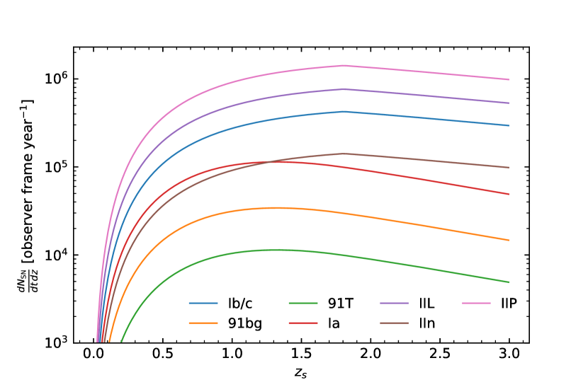
We draw a redshift for each supernova from the functions shown in Figure 1. The normalized Figure 1 curves give the redshift probability density function for supernova type ,
| (30) |
where is the source redshift. For each supernova subtype, we assume that the spectral evolution is described by a template with one parameter (the overall normalization), and we use the realized to set its value assuming the Planck Collaboration et al. (2016) cosmology described in Section 1. With sampling prescriptions for and , we can realize supernovae at random. Table 1 lists the references for our supernova templates, rates, and luminosity functions.
2.4 Host Galaxies
The connection between supernovae and their host galaxies is of critical importance to time delay cosmology with gLSNe, as lensed host galaxy arcs will provide significant leverage on lens models (e.g., Suyu et al., 2017). Here we describe an empirical model of the supernova-host galaxy connection that we use to realize hosts for each supernova in our simulation. Throughout this section, we assume that deflector, lens galaxy, and supernova parameters have already been sampled as described in Sections 2.1, 2.2, and 2.3. We consider three types of host galaxies: elliptical galaxies, which have almost no ongoing star formation, S0/a-Sb galaxies, which have a moderate level of ongoing star formation, and late-type/sprial galaxies, which have vigorous ongoing star formation. As an ansatz, we take the light profiles of the host galaxies in the absence of lensing to be Sérsic functions with , respectively. Only normal SNe Ia and SN1991bg-like events have been observed to be hosted by elliptical or S0/a-Sb galaxies. Based on measured rates, we assume these two subclasses of thermonuclear supernovae have a 30% chance of being hosted by an elliptical, a 35% chance of being hosted by a S0/a-Sb, and a 35% chance of being hosted by a late-type/spiral, roughly consistent with the results of Han et al. (2010), Li et al. (2011), Hakobyan et al. (2012), and Smith et al. (2012). In our simulations, Type Ib/c, Type IIP, Type IIL, Type IIn, and SN 1991T-like supernovae can only be hosted by late-type/spiral galaxies. For simplicity, we assume the spectra of the host galaxies are given by the following Kinney et al. (1996) templates: Elliptical (elliptical), Sc (S0/a-Sb), and Starburst (late-type/spiral).
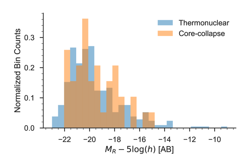
We draw the host galaxy luminosities from two separate luminosity functions: one for the hosts of thermonuclear supernovae (SNe Ia, SN 1991bg-like, and SN 1991T-like events) and one for the hosts of core-collapse supernovae. We construct both of our luminosity functions using supernovae discovered by the Palomar Transient Factory (PTF; Law et al., 2009). PTF discovered thousands of supernovae to and obtained spectral confirmation of many of them in a relatively unbiased manner. For the core-collapse supernovae, we draw the cosmology-independent host galaxy rest-frame -band absolute magnitude at random from the sample of Arcavi et al. (2010) confined to to limit the effects of peculiar velocities and to ensure a complete sample. For the thermonuclear events, we use a catalog compiled by E. Y. Hsiao and P. E. Nugent (private communication) drawn from the PTF discoveries that overlapped with fields observed by SDSS and BOSS.
Figure 2 shows the luminosity functions of core-collapse and thermonuclear supernova host galaxies used in the present calculations. The host galaxy redshift is fixed to the redshift of the supernova,
| (31) |
The sampled values of and fix the normalization of the host galaxy spectral template and the host galaxy Sérsic profile amplitude under the assumption of a Planck Collaboration et al. (2016) cosmology.
Following Shen et al. (2003), we take the sizes and intrinsic brightnesses of galaxies to be correlated via the “size-luminosity relation,”
| (32) |
where is the effective radius of the host galaxy Sérsic profile and and are global parameters. Shen et al. (2003) find that for elliptical galaxies, is related to via
| (33) |
where
| (34) |
Fitting to data from SDSS, Shen et al. (2003) find and . For S0/a-b and late-type/spiral galaxies, they find
| (35) |
where fitting the SDSS data give , , , and . The dispersion in the size-luminosity relation is given by
| (36) |
for all galaxy types, with and . Having calculated and given , we can sample a value of using Equation 32.
The next steps are to draw the host galaxy ellipticity and position angle . We take the host galaxy orientation to be random,
| (37) |
and to draw ellipticities, we use the results of the Cosmic Evolution Survey (COSMOS; Scoville et al., 2007). COSMOS is a survey designed to probe the correlated evolution of galaxies, star formation, active galactic nuclei, and dark matter with large-scale structure. Our access point to COSMOS is the Advanced Camera for Surveys General Catalog (ACS-GC; Griffith et al., 2012). ACS-GC is a photometric and morphological database containing fits of structural parameters to publicly available data obtained with the Advanced Camera for Surveys (ACS) instrument aboard HST. The catalog was created using the code Galapagos (Häußler et al., 2007, 2011), which incorporates the source extraction and photometry software SExtractor (Bertin & Arnouts, 1996) and the galaxy light profile fitting algorithm GALFIT (Peng et al., 2002). ACS-GC contains photometry and structural parameters for approximately 305,000 objects (both compact and extended) from COSMOS. The COSMOS images were taken with the Wide Field Camera (WFC) on ACS, through the F814W filter, a broad -band filter spanning the wavelength range 7000 – 9600Å, with a scale of 0.05 arcsec pixel-1 and a resolution of 0.09′′ FWHM.
We apply the cuts of Gupta et al. (2016) to create a list of potential supernova host galaxies from the ACS-GC. We further subdivide this list into two groups: “early” and “late”-type galaxies, having fitted values of the Sérsic index in the ACS-GC of and , respectively. For elliptical hosts, we draw at random from the fitted ellipticity values of the “early” group, and for S0/a-b and late-type/spiral hosts, we draw at random from the fitted ellipticity values of the “late”-type group.
The last parameters to draw are the unlensed coordinates of the host galaxy centroid and . Here we take the PDF of supernova positions within the host galaxy to be directly proportional to the light profile, an assumption that has been borne out by observational studies that show supernova positions follow host light (Kelly & Kirshner, 2012). Thus we sample offsets and at random from the host galaxy light profile, then take
| (38) | ||||
| (39) |
The host galaxy light profiles follow a Sérsic function, defined as,
| (40) |
where is an ellipticity-free, host galaxy-centered radial coordinate and is a constant scalar solution to the equation
| (41) |
in which is the Gamma function and is the incomplete Gamma function.222An exact, computationally inexpensive method of calculating for a given value of is to evaluate in scipy. To sample a position at random from the surface brightness profile we first draw two random deviates and uniformly,
| (42) | ||||
| (43) |
Using the sampled , we solve the following equation333See Footnote 2, but with the substitutions and . for :
| (44) |
then convert into the radial coordinate (see, e.g., Graham & Driver, 2005),
| (45) |
We can now write the ellipticity-free host offsets and as
| (46) | ||||
| (47) |
We add ellipticity to obtain and ,
| (48) | ||||
| (49) |
Finally, we account for the position angle of the host galaxy by applying a rotation matrix,
| (50) |
With sampling prescriptions for and , we can realize host galaxy light profiles at random.
2.5 Sky Distribution
We assign a sky location to each system realized in our simulation, which in turn determines the sampling, signal-to-noise ratio, and filters of its simulated photometry. The sky location also controls the amount of Milky Way dust extinction each system experiences (see Section 2.6). To randomly assign a sky position to a gLSN system, we draw two random deviates and uniformly,
| (51) | ||||
| (52) |
We then convert these to equatorial coordinates (right ascension) and (declination) via
| (53) |
and
| (54) |
This sampling prescription ensures that systems are distributed uniformly over the celestial sphere.
2.6 Extinction
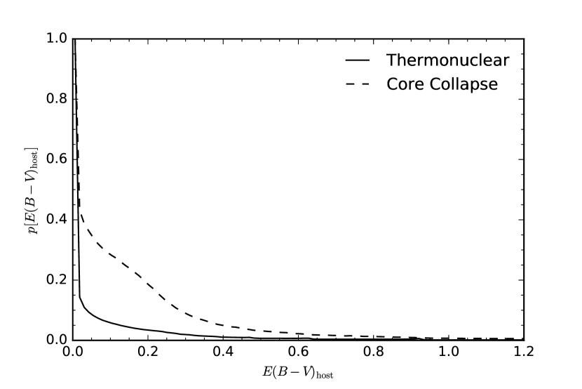
After randomly assigning a sky location to each gLSN system, we use the extinction maps of Schlegel et al. (1998) to calculate the associated Milky Way reddening value, . We then apply the extinction to the observer-frame spectral time series of the supernova images using a Cardelli et al. (1989) reddening law with . In addition to extinction by dust in the Milky Way, gLSNe can suffer extinction by dust in their host galaxies. Here we assume the host galaxy reddening is distributed according to the thermonuclear and core-collapse extinction distributions of Hatano et al. (1998) for galaxies at random orientations, shown in Figure 3. We apply host extinction to the rest-frame spectral time series of the supernova images using a Cardelli et al. (1989) reddening law with , the measured Galactic value. Amanullah et al. (2015) showed that there is significant diversity in the value of for the observed host galaxy extinction in Type Ia supernovae and similar conclusions were reached for certain types of core-collapse SNe in Stritzinger et al. (2018). In particular, lower values of are often found, (see Bulla et al., 2018, for a proposed explanation). By selecting a value of on the upper range observed, we are assuming a relatively large attenuation by dust, , i.e., a conservative estimate of the SN brightness. We neglect of extinction by dust in the lens galaxies, which may reduce yields by making lensed images fainter. SN iPTF16geu showed evidence of extinction due to lens galaxy dust at sub-kpc offsets (Goobar et al., 2017), but with only one event the frequency and spatial distribution of lens galaxy dust remain unclear. ZTF and LSST will be able to better constrain lens galaxy dust extinction by producing large samples of gLSNe Ia.
2.7 Simulated Surveys
To simulate realistic light curves and pixel cutouts of our lens systems as they would appear in a survey, we must account for the survey’s unique observing strategy and conditions, instrumental properties, and visit schedule. To do this, we use the outputs of software tools that run survey simulations with given science driven desirables; a software model of the telescope and its control system; and models of weather and other environmental variables. Such simulations produce observation histories, which are records of times, pointings and associated environmental data and telescope activities throughout a simulated survey. These histories can be examined to assess whether a simulated survey would be useful for any particular purpose or interest. We adopt a common format for survey observation histories, consisting of a table with the following columns:
-
1.
field: The field ID of the observation.
-
2.
filter: The filter in which the observation was taken.
-
3.
time: The MJD at which the observation began (the shutter-open time).
-
4.
exptime: The integration time of the exposure.
-
5.
sky_counts_per_pixel: The sky counts (in electrons) in each pixel. This is not a count rate, but the counts integrated over the entire exposure. This column can optionally also include counts due to other spatially uniform Poisson backgrounds, such as dark current.
-
6.
psf_sigma: The standard deviation (in arcseconds) of the PSF, modeled as a Gaussian.
-
7.
ra: Right ascension of the center of the pointing.
-
8.
dec: Declination of the center of the pointing.
-
9.
night (optional): An integer ID specifying the night of the survey in which the observation was taken, used for grouping and stacking observations.
In addition to the observation histories, we specify instrumental properties with the following parameters:
-
1.
pix_scale: The plate scale of the camera (arcsec / pixel).
-
2.
read_noise: The read noise of the camera, in electrons.
-
3.
field_of_view: The field of view of the imager, in deg2.
-
4.
collecting_area: The collecting area of the telescope, in cm2.
In this work, we consider two surveys: ZTF and LSST, the two largest imaging surveys at optical wavelengths during the periods 2018–2021 and 2021–2032, respectively. In the following subsections, we describe these surveys and the operations simulations that we use to realize their data.
2.7.1 The Zwicky Transient Facility
The Zwicky Transient Facility (ZTF) is an ongoing time-domain imaging survey observing a minimum of 15,000 deg2 in and -band ( deg) every 3 nights to a depth of at least 20.5 mag, with transient alerts released in real-time to the public.444Public alerts can be retrieved from http://ztf.uw.edu. In March 2018, ZTF began science operations, replacing its predecessor, the intermediate Palomar Transient Factory (iPTF), on the 1.2-meter Oschin-Schmidt telescope (P48) at Palomar Observatory near San Diego, California. The chief advance of ZTF over iPTF is a new wide-field camera developed for the survey (Smith et al., in preparation). With its 47 deg2 field of view, the ZTF camera can survey 3,750 deg2 per hour to , making it roughly an order of magnitude faster than iPTF. In addition to the 15,000 deg2 public survey, a subset of 1,600 deg2 is currently monitored six times per night in two filters as a part of the ZTF partnership survey. Half of the survey area is also monitored in -band every 4 nights. The remaining 20% of the survey time is allocated to proposals from collaboration members affiliated with the California Institute of Technology (Caltech) on a competitive basis. We simulate data from all three ZTF programs in the present work using the simulated ZTF survey of Bellm et al. (in preparation), which uses the same scheduler as the actual survey. The scheduler uses Gurobi optimization,555http://www.gurobi.com/ a technique for integer programming, to maximize the number of images, weighted by the volume surveyed per image, observed in acceptable cadence windows, while maintaining a balance between the public, Partnership, and Caltech surveys. While the observing sequence determined by the scheduler in the simulation is reliable, the observing conditions used by the simulation are overly optimistic, predicting limiting magnitudes 21.5 in all filters. In reality, ZTF can only reach a limiting magnitude of 20.5 in any filter in a 30-second exposure. Therefore, in our simulation, we set the seeing FWHM to 2′′, the survey median, and the limiting magnitude to 20.5 for all observations.
2.7.2 The Large Synoptic Survey Telescope
The Large Synoptic Survey Telescope is a planned imaging experiment that will conduct at least two interleaved surveys: a “wide-fast-deep” (WFD) survey covering roughly 20,000 deg2 in every 2–3 weeks with 30 second exposures , and a “deep drilling” survey covering a smaller area at a significantly higher cadence (LSST Science Collaborations et al., 2017). A new 8m-class telescope and camera with a 9.6 deg2 field-of-view and 0.2′′ pixels, located on the Cerro Pachón ridge in northern Chile, are currently under construction to carry out the survey. First light and commissioning operations will begin in 2021, followed by science operations in 2022. The survey will collect data for 10 years.
Several detailed candidate observing strategies have been proposed for LSST. In this analysis we evaluate two of the major ones from the perspective of gLSN science: a nominal observing strategy, known as minion_1016, and a leading alternative, known as altsched. minion_1016 divides its time between five interleaved surveys: a “Universal” WFD survey (85.1%), a proposal to monitor the North Ecliptic Spur (6.5%), a proposal to monitor the Galactic plane (1.7%), a proposal to monitor the South Celestial Pole (2.2%), and a proposal to monitor 5 9.6 deg2 “deep-drilling” fields (4.5%). The median effective seeing (FWHM) for all proposals in -band is 0.93′′. The median single-visit depths for the WFD fields are (23.14, 24.47, 24.16, 23.40, 22.23, 21.57) in the bands.
The minion_1016 simulation was performed using the software tool OpSim (Delgado et al., 2014). OpSim uses a greedy algorithm that chooses the best observation at a given time (according to a merit function based on the input science goals), with no look-ahead or long-term strategy. altsched, on the other hand, takes a simpler approach, following a pre-programmed path with no merit function. altsched attempts to observe fields at low airmass by observing only on the meridian, optimizing the signal-to-noise ratio (SNR) of the observations. Like minion_1016, altsched retains a dual-visit per night requirement for transient artifact rejection and asteroid orbit linkage, but the two visits are taken in different filters, so colors can be obtained on all objects. altsched simulations of SN Ia light curves have shown the alternative cadence can lead to significantly better light curve sampling than minion_1016. In Section 4, we evaluate both minion_1016 and altsched for the LSST gLSN science case.
2.8 Imaging, Photometry, and Calibration
To realize images and photometry of our simulated gLSN systems as they would appear in the mock surveys described in Section 2.7, we have developed an image-simulation pipeline based on the open-source astronomical image simulation code GalSim (Rowe et al., 2015) and the gravitational lensing code glafic (Oguri, 2010). For a given arrangement of supernova, host galaxy, and lens, we first solve the lens equation using glafic to determine the magnifications, time delays, multiplicities, and locations of the lensed supernova images. We then use glafic to solve the lens equation again for the magnification and surface brightness profile of the lensed host galaxy. With this information, we use GalSim to model the entire system. In GalSim parlance, we model each lensed supernova image as a DeltaFunction, the lens galaxy as a Sersic, and the lensed host galaxy surface brightness profile as an InterpolatedImage. We convolve the model with a Gaussian model of the PSF, the width of which is provided by the survey simulation (see Section 2.7). We refer to the noiseless convolved model as and the pixel values of the corresponding model image as . To generate an image for viewing, we add CCDNoise to the model consisting of Gaussian read noise, Poisson sky background, and Poisson source noise.
We perform photometry using a matched filter, following Bridle et al. (2009). We assume we have a filter that perfectly matches the shape of the source and is normalized to 1, i.e., . We calculate the measured signal as a weighted sum of the image and the filter, via
| (55) |
and we define the noise as the square-root of the signal variance,
| (56) |
where
| (57) |
In Equation 57, RN is the read noise per pixel in e- and is the flux in e- from the background (i.e., the sky, dark current, etc.) at pixel . Finally, we determine the image zeropoint ZP via
| (58) |
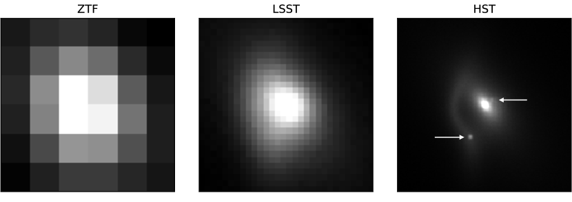
where is the apparent magnitude of the source through some filter in the AB system. Figure 4 shows three example simulated images of the same gLSN system generated using our pipeline, taken with three different instruments under representative observing conditions.
To increase our sensitivity to faint transients, we stack observations taken in the same filter in a single night. For minion_1016, this has the effect of combining the two exposures taken in the same filter in a 30-minute window to reject moving objects into a single observation with a signal-to-noise ratio roughly a factor of larger. For altsched, the stacking has no effect, as the strategy performs revisits to reject moving objects in different filters to obtain colors. For ZTF, stacking has no effect on the public MSIP data, which has a typical revisit time of 3-4 days in each filter. However, the stacking significantly boosts survey depth in the high-cadence Partnership fields and the Caltech survey. In some regions of these proprietary surveys, a single field may be observed as many as six times per night in a single filter, leading to a potential improvement in depth of mag over the nominal limiting magnitude of 20.5 in all filters. We apply the discovery technique discussed in the next section (Section 2.9) to the stacked, not raw, data.
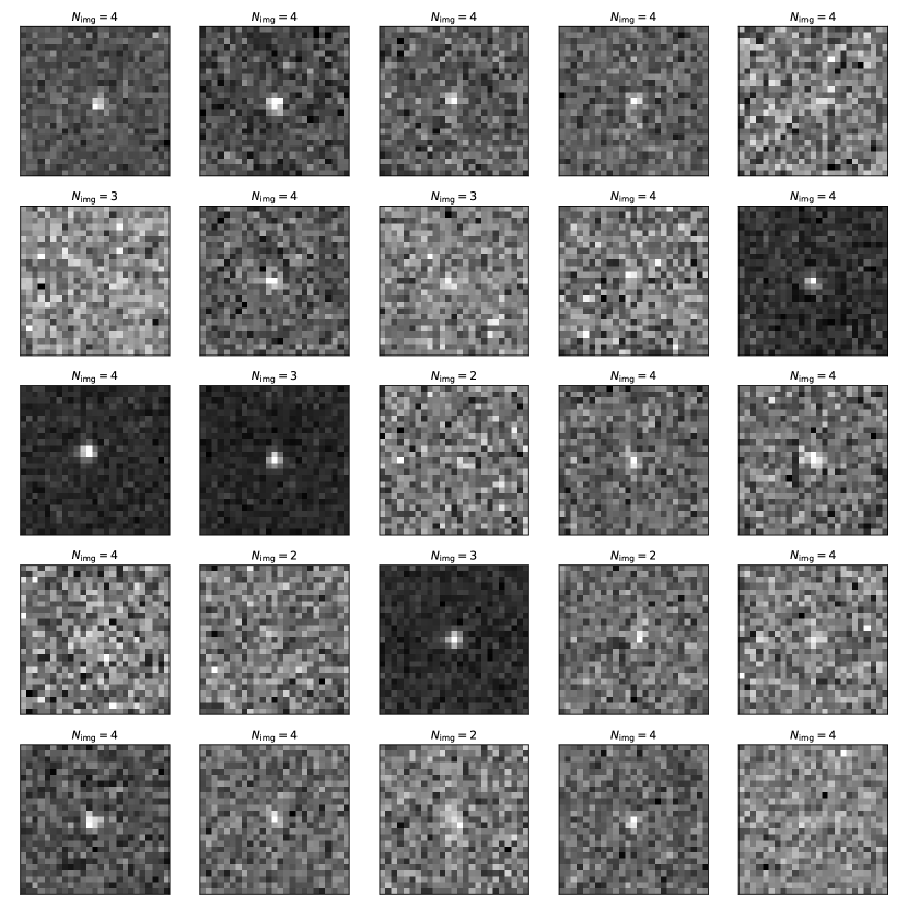
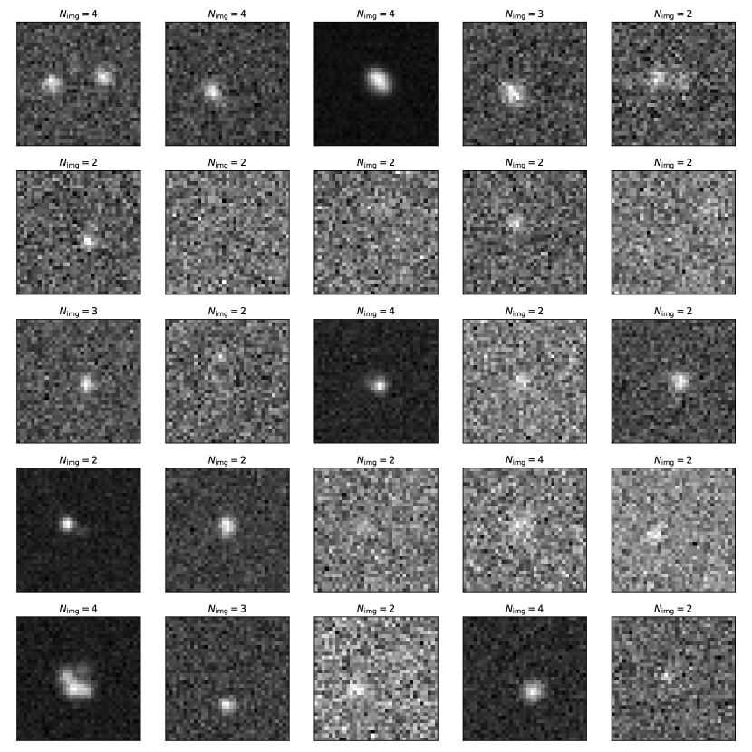
An important simplification in our simulations is that we treat gLSN images as a single object when performing photometry. The effect of this assumption is that we can realize a single light curve for each gLSN system, the flux of which is the summed flux of the individual images. For ZTF, this is a reasonable assumption, as the large pixels of the detector and the 2′′ seeing at Palomar Observatory ensure gLSNe cannot be resolved (see Figure 5). For LSST, as Figure 6 shows, this assumption should in most cases. For the cases where the assumption does not hold, and the multiple images of a gLSN are resolved, the transient can be detected as two or more bright, nearby transients, as proposed by Oguri & Marshall (2010). For simplicity, we also assume perfect image subtractions. The main implication of this assumption is that photometric accuracy and source detection are unaffected by proximity to the cores of bright lens galaxies.
2.9 Discovery Technique
We simulate the detection and photometric classification of gLSNe using the technique described in Goldstein et al. (2018). The strategy rests on three observational facts. First, normal Type Ia supernovae (SNe Ia) are the brightest type of supernovae that have ever been observed to occur in elliptical galaxies (Maoz et al., 2014). Second, the absolute magnitudes of normal SNe Ia in elliptical galaxies are remarkably homogenous, even without correcting for their colors or lightcurve shapes , with a component of the population being underluminous (Li et al., 2011). Finally, due to the sharp 4000Å break in their spectra, elliptical galaxies tend to provide accurate photometric redshifts from large-scale multi-color galaxy surveys such as SDSS.
A high-cadence, wide-field imaging survey can leverage these facts to systematically search for strongly lensed supernovae in the following way. First, by spatially cross-matching its list of supernova candidates with a catalog of elliptical galaxies for which secure photometric redshifts have been obtained, supernovae that appear to be hosted by elliptical galaxies can be identified. The hypothesis that one of these supernovae actually resides in its apparent host can be tested by fitting its broadband light curves with an SN Ia spectral template (as SNe Ia are the only types of supernovae that occur in ellipticals) fixed to the photometric redshift of the galaxy and constrained to obey , a liberal absolute magnitude range for SNe Ia, assuming a fiducial cosmology. If the transient is a lensed supernova at higher redshift, then the spectral template fit will fail catastrophically, as the supernova light curves will be strongly inconsistent with the redshift and brightness implied by the lens galaxy.
We use SALT2 (Guy et al., 2007), a parametrized SN Ia spectral template that is the standard tool for placing SNe Ia on the Hubble diagram, to perform this technique. The template possesses four parameters: , , , and , encoding a reference time, an overall SED normalization, a supernova “stretch,” and a color-law coefficient, respectively. The flux of the template is given by
| (59) |
where and are eigenspectra derived from a training sample of measured SN Ia spectra and is the average color-correction law of the sample (see Guy et al., 2007, for details). The template aims to model the mean evolution of the SED sequence of SNe Ia and its variation with a few dominant components, including a time independent variation with color, whether it is intrinsic or due to extinction by dust in the host galaxy (or both). Finally, we draw a random reference time for the system uniformly over the duration of the survey,
| (60) |
where and are the times of the survey’s first and last observations, respectively.
We realize broadband photometry of each blended gLSN Ia using the technique described in Section 2.8. Starting from the first observation of the SN Ia, we fit the light curve with SALT2, fixed to the redshift of the lens galaxy (assumed to be known either as a photometric or spectroscopic redshift) and fixed to obey at that redshift (effectively a constraint on ). Additionally, we enforce bounds of on and on , values characteristic of normal SNe Ia (Scalzo et al., 2014). We use the CERN minimization routine MIGRAD (James & Roos, 1975) to fit the data. If the light curve has at least one data point that is at least discrepant from the best fit and at least 4 data points with S/N , then the object is marked “detected.” If not, then the next observation is added and the process is repeated until the object is detected or all observations are added, resulting in a non-detection.
2.10 Importance Sampling, Sample Weighting, and Rate Calculation
We perform a separate Monte Carlo simulation for each survey and supernova type, running each simulation until gLSN systems are discovered. In each iteration of the simulation we realize one supernova behind the sampled lens in the lensing area of influence. We run each ZTF simulation for iterations, and we run each LSST simulation for iterations. The ZTF simulations require more iterations to converge as ZTF is shallower than LSST, so any given system is less likely to be detected. To reduce shot noise in our results, we use importance sampling to sample lens and source redshifts, the distributions of which contain almost no probability mass in the crucial region . Therefore, each system has an associated importance weight factor ,
| (61) |
where and are the true densities of and (Equations 14 and 30), and are the sampling densities, is the ratio of sky area imaged by the survey to sky area covered in the simulation, and is the factor by which the supernova rate must be multiplied to yield one supernova of the given subtype with per year in the “lensing area of influence” of the lens. We take the sampling densities to be uniform,
| (62) | ||||
| (63) |
where and are the minimum and maximum supernova redshifts considered in the simulation, respectively. We assume the lenses are uniformly distributed across the sky, so the areal correction factor can be calculated by dividing the total number of lenses in the survey area by the number of lenses realized in the simulation,
| (64) |
where we have integrated Equation 11 to estimate the total number of lenses in the survey area. In Equation 64, is the area of the survey in steradians and and are the minimum and maximum lens velocity dispersions considered in the simulation, respectively.
The number of supernovae per year behind the lens’s area of influence is determined by integrating the observer-frame supernova redshift function (Figure 1) from or (whichever is larger) to and multiplying by the ratio of the lens’s area of influence to the full-sky area. Taking and , we have
| (65) |
The weights specify the contribution of a given discovered system to the overall gLSN discovery rate, and have units of [year-1]. The summed weights provide a Monte Carlo estimate of the gLSN discovery rate,
| (66) |
where is the total discovery rate (in year-1). As with any Monte Carlo estimator, the precision of increases as the square root of the number of samples . The above scheme is roughly times more efficient than sampling all of the parameters of the model brute-force.
3 Results
Table 2 shows the gLSN discovery rates of each simulated survey. Our calculations suggest that under nominal survey operations, ZTF should discover at least 8.60 gLSNe per year, of which at most 4.1% are Type Ib/c, 2.0% are SN 1991T-like, 3.7% are Type IIL, 14.3% are Type Ia, 32.1% are Type IIP, 0.2% are SN 1991bg-like, and at least 43.6% are Type IIn. We find that the minion_1016 LSST observing strategy should discover at least 380.60 gLSNe per year, of which at most 12.6% are Type Ia, 1.6% are SN 1991T-like, 23.3% are Type IIP, 4.1% are Type Ib/c, 3.4% are Type IIL, 0.2% are SN 1991bg-like, and at least 55.0% are Type IIn. The altsched observing strategy should discover at least 341.27 gLSNe per year, of which at most 4.7% are Type Ib/c, 3.8% are Type IIL, 13.9% are Type Ia, 26.7% are Type IIP, 1.8% are SN 1991T-like, 0.3% are SN 1991bg-like, and at least 45.3% are Type IIn. The Type IIn rates are given as lower limits because gLSNe IIn can be detected in both ZTF and LSST beyond , the maximum redshift in our simulations, but their rate at is highly speculative.
| SN Type | ZTF | LSST (minion_1016) | LSST (altsched) |
|---|---|---|---|
| Type Ia | 1.23 | 47.84 | 47.42 |
| Type IIP | 2.76 | 88.51 | 91.06 |
| Type IInaaLower limit. | 3.75 | 209.31 | 166.54 |
| Type IIL | 0.31 | 11.69 | 13.10 |
| Type Ib/c | 0.36 | 14.00 | 16.15 |
| SN 1991bg-like | 0.02 | 0.79 | 0.89 |
| SN 1991T-like | 0.17 | 5.41 | 6.09 |
| TotalaaLower limit. | 8.60 | 380.60 | 341.27 |
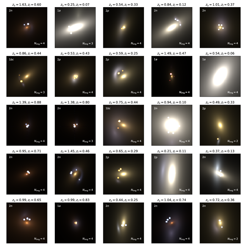
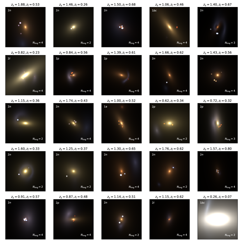
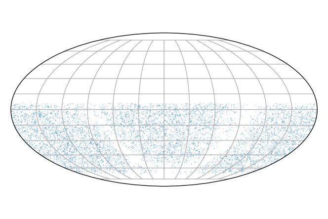
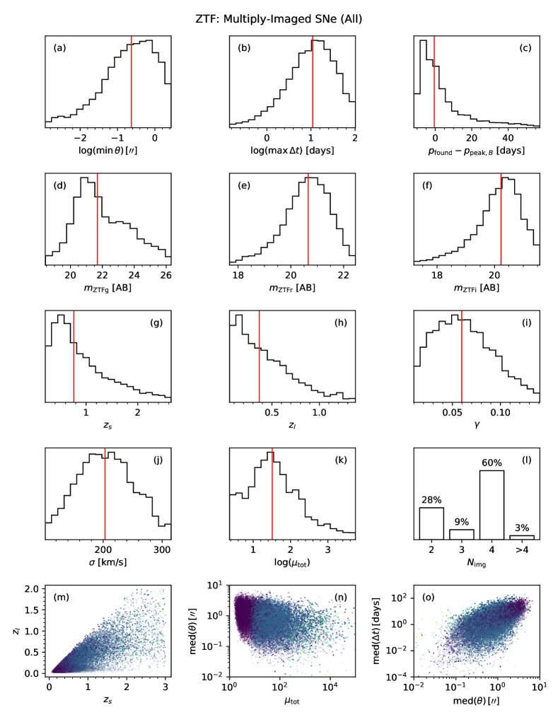
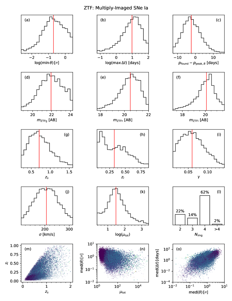
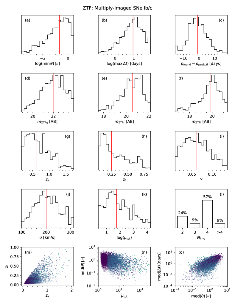
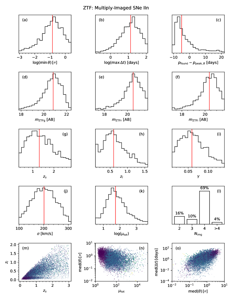
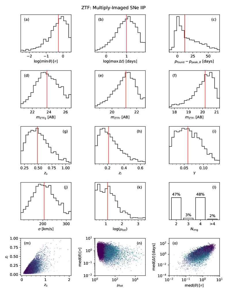
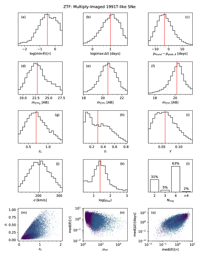
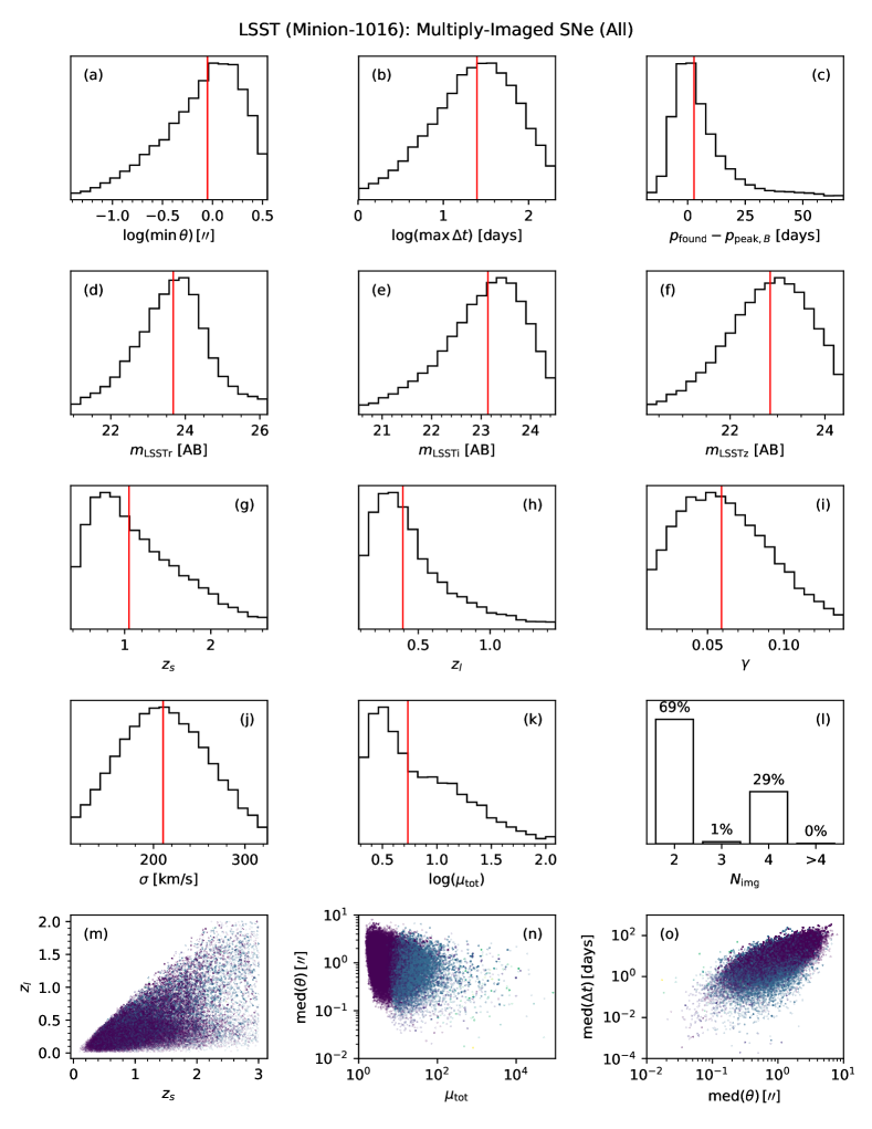
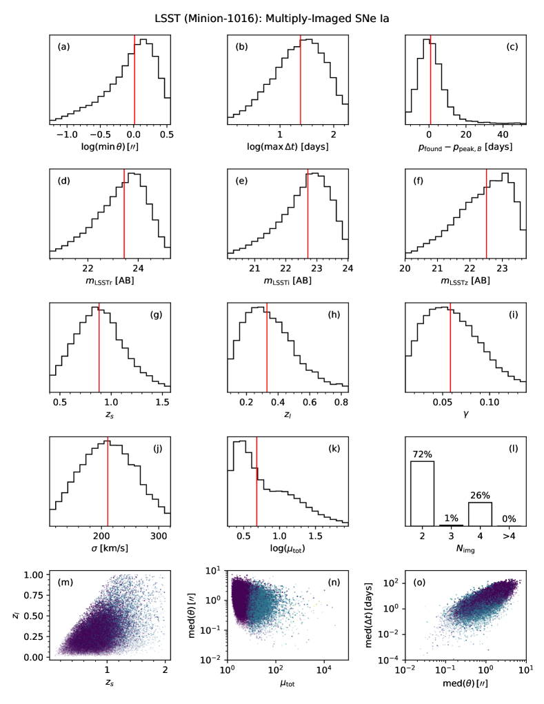
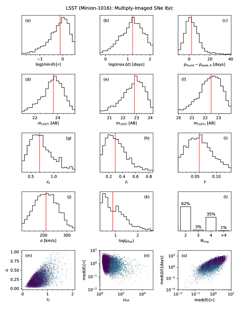
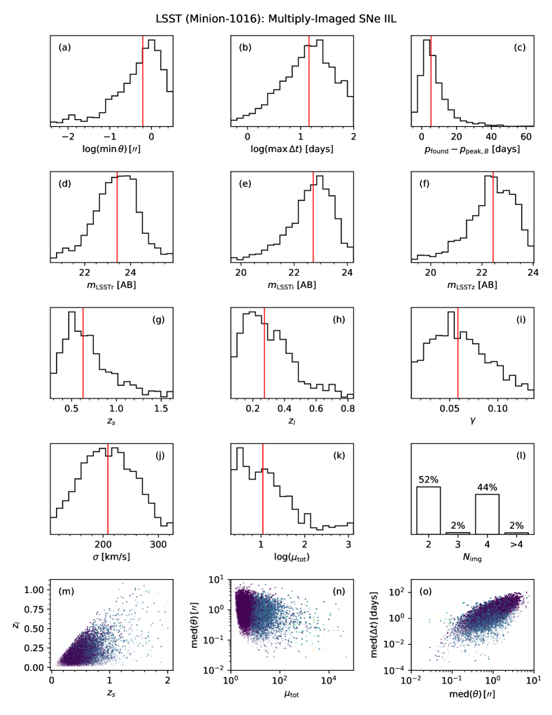
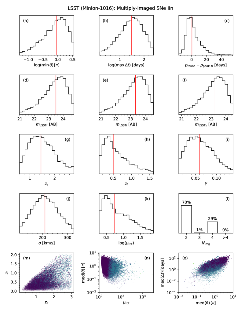
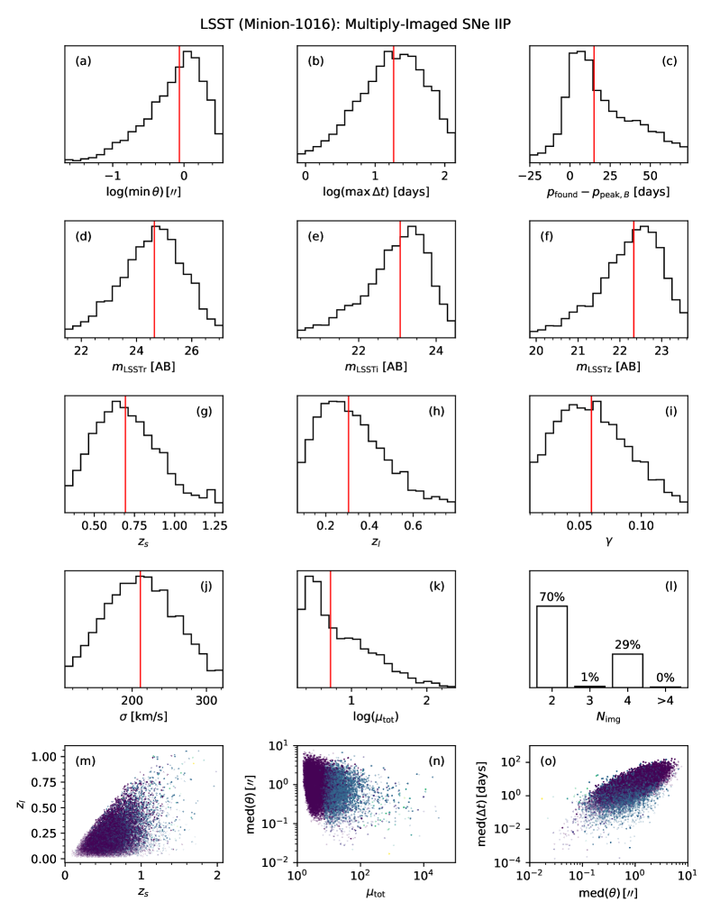
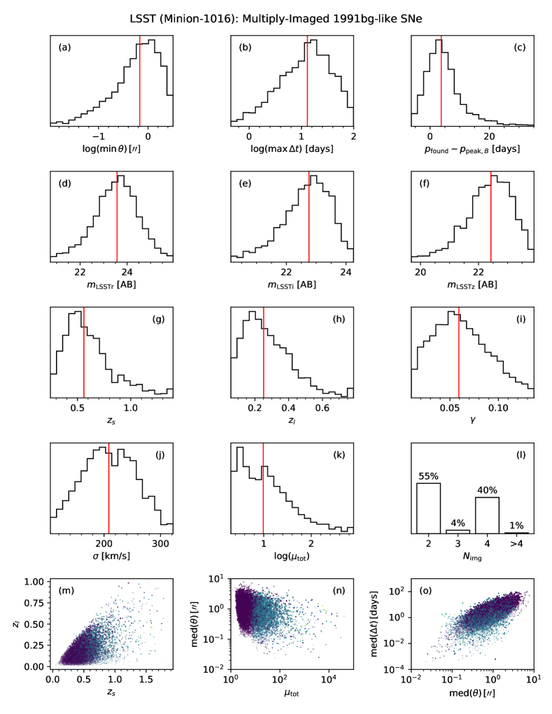
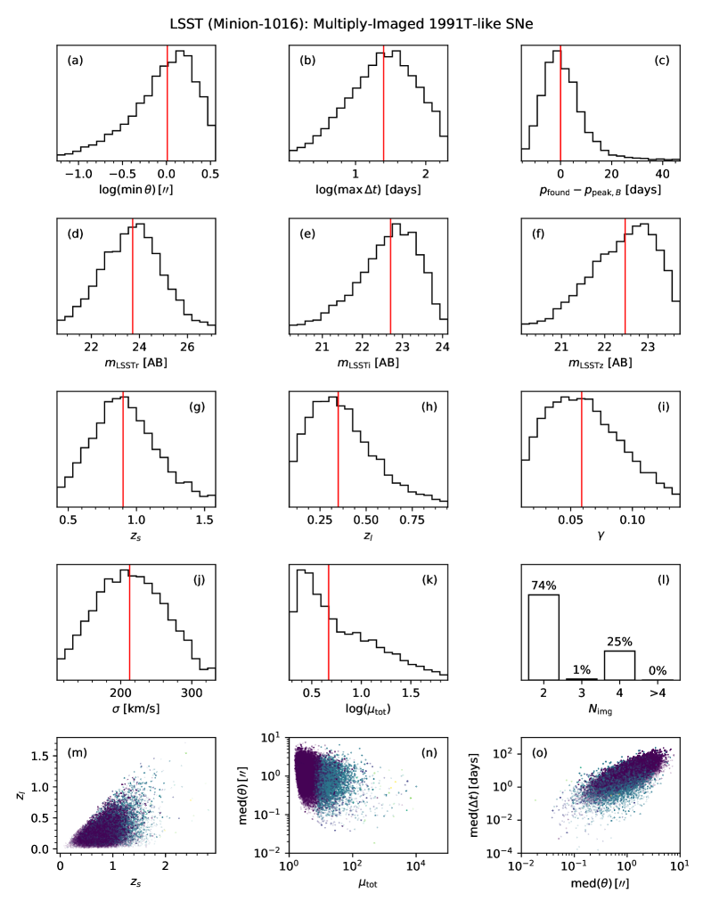
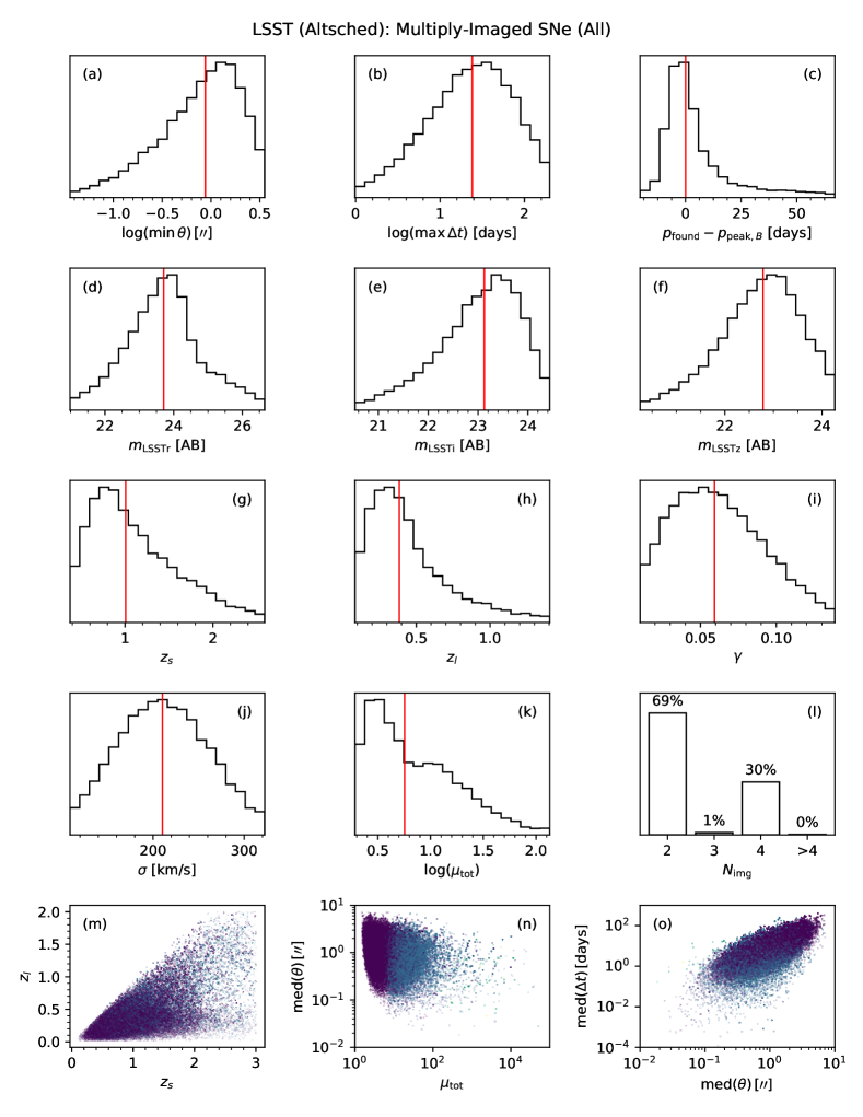
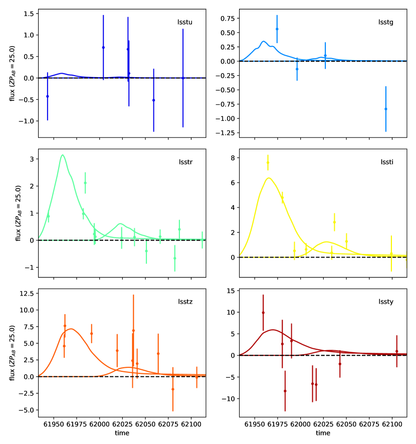
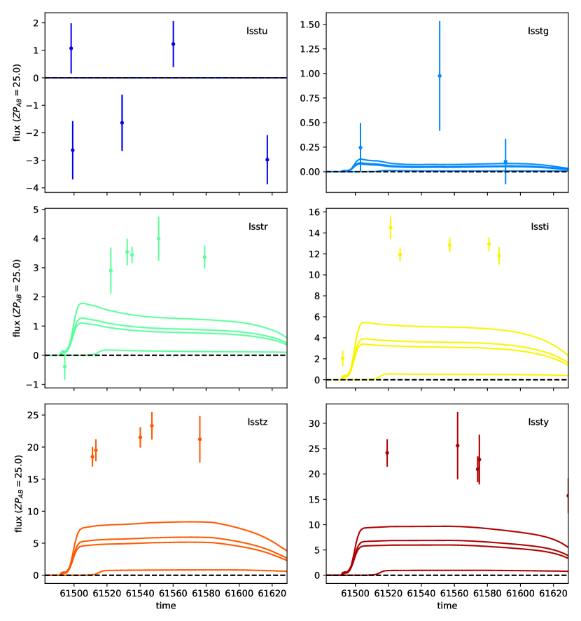
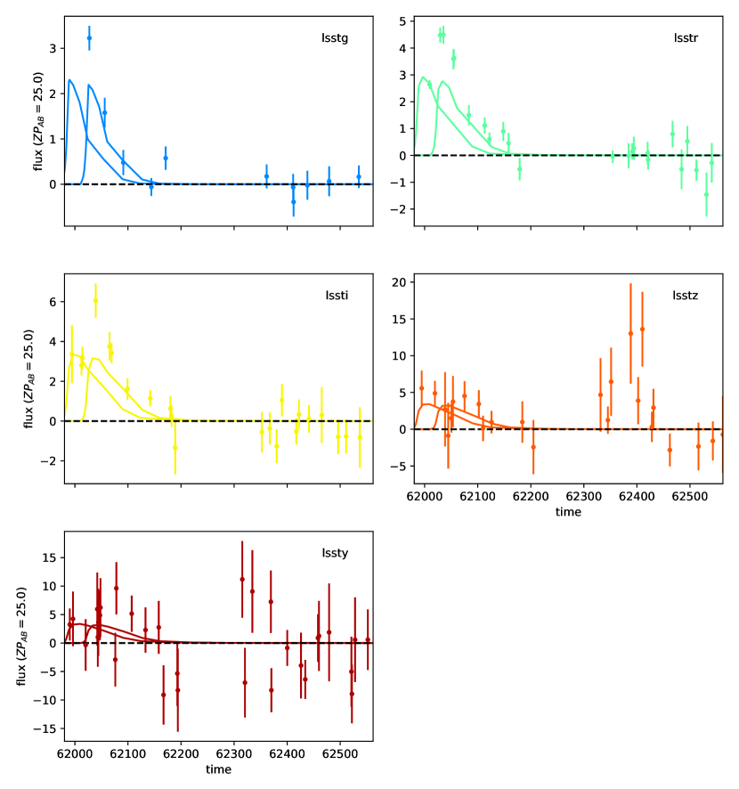
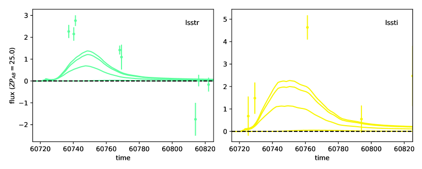
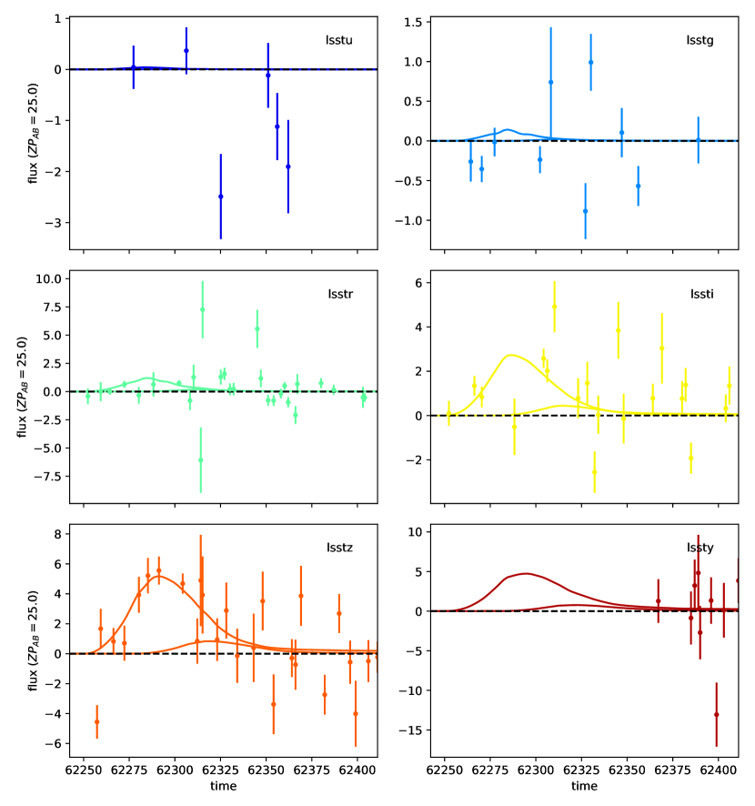
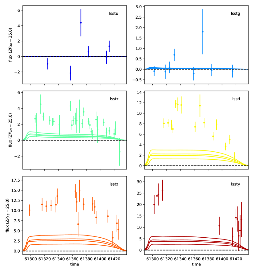
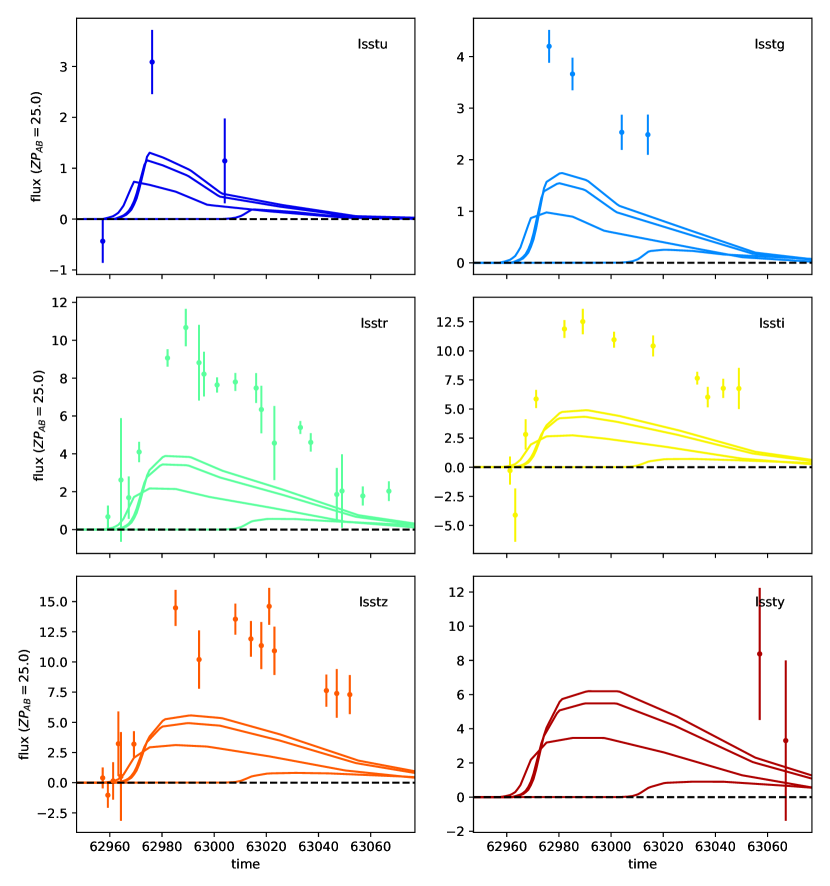
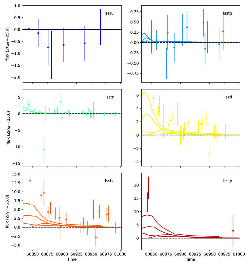
Color-composite images of randomly selected gLSNe, drawn in proportion to their weights, discovered by ZTF and LSST (minion_1016) are shown in Figures 7 and 8, respectively. Figures 9 and 10 show the sky distributions of detected gLSNe. Figures 11 – 25 summarize the results of our Monte Carlo simulations, presenting the distributions of several key observables and parameters of detected systems. Table 3 describes the subpanels in each figure, and red lines in histogram panels indicate medians. Figures 26 – 35 show multi-band light curves of gLSNe from ZTF and LSST. In those figures, the solid lines reflect the true underlying light curves of each image, while the photometric data are realized from the sum of the images. The ZTF photometry is unstacked, reflecting the survey’s high intranight cadence, whereas the LSST photometry is combined nightly into single point per filter for clarity. Figure 39 shows distributions of lensed host galaxy apparent magnitudes and separations (relative to the lens centroid) in units of . If the lens-host centroid distance is less than , there is a strong likelihood that the host galaxy is multiply imaged and can thus provide useful constraints on the lens model.
Figures 7 – 8, 11, 17, and 25 show that ZTF and LSST are sensitive to different populations of gLSNe. ZTF gLSNe have a median , , , days, , and . LSST gLSNe have a median , , , days, , and . Synthesizing this information, the ZTF gLSNe tend to be more compact, highly magnified, and have shorter time-delays than their LSST counterparts. Additionally, ZTF gLSNe are more likely to be quads than gLSNe from LSST. The gLSN iPTF16geu discovered by ZTF’s predecessor iPTF was broadly consistent with this picture: it was a compact , highly magnified , quad with short time delays ( day). The gLSNe from LSST will be better suited to time-delay cosmology. Their longer time delays and wider separations will enable more precise constraints on H0 and better models of the mass profile. However, they will be fainter, and thus require larger telescopes and more observing time for follow-up observations. Table 4 shows that just 10% of the gLSNe ZTF will find will come from the public data alone. The proprietary data, notably the high-cadence data and the -band survey, will be critical for discovering gLSNe.
| Subpanel | Description |
|---|---|
| a | The smallest angular separation, in arcseconds, between two images in the system (alternatively, the angular resolution required to completely resolve the system). |
| b | The largest time delay between two images in the system. |
| c | The rest-frame phase of the blended light curve on the date of discovery relative to rest-frame -band maximum. |
| d | Peak observer-frame AB magnitude of the gLSN in (ZTF) or (LSST). |
| e | Peak observer-frame AB magnitude of the gLSN in (ZTF) or (LSST). |
| f | Peak observer-frame AB magnitude of the gLSN in (ZTF) or (LSST). |
| g | The source redshift. |
| h | The lens redshift. |
| i | The magnitude of the external shear. |
| j | The SIE velocity dispersion. |
| k | The total lensing amplification of the gLSN images. |
| l | The number of gLSN images in the system. |
| m | The correlation between source and lens redshift, color coded by image multiplicity. Purple points correspond to double images, blue to quads, and redder colors to systems with more than four images. |
| n | The correlation between total magnification and image separation, color coded as (m). |
| o | The correlation between median image separation and median time delay, color coded as (m). |
| SN Type | [%] | High Cadence [%] | MSIP Only [%] |
|---|---|---|---|
| Type Ia | 77.7 | 77.3 | 12.4 |
| Type IIP | 82.0 | 73.9 | 10.5 |
| Type IIn | 71.3 | 73.1 | 16.2 |
| Type Ib/c | 80.4 | 76.8 | 10.8 |
| Type IIL | 81.1 | 75.1 | 10.7 |
| SN 1991bg-like | 81.7 | 75.6 | 9.9 |
| SN 1991T-like | 77.3 | 75.5 | 13.0 |


4 Discussion
4.1 Comments on the LSST Observing Strategy
Broadly speaking, candidate observing strategies for LSST can be arranged on a spectrum in which area and season length are traded for sampling and depth. In this analysis we have investigated strategies from both ends of this spectrum. minion_1016 covers a large area with relatively poor light curve sampling, while altsched covers a smaller area with better sampling and greater depth. Table 2 shows that the nominal LSST observing strategy minion_1016 discovers roughly the same number of gLSNe as the alternative strategy altsched, and Figures 17 and 25 show that the greatest difference in the gLSNe discovered under the two strategies is the discovery phase (see panel (c) of both figures). altsched discovers gLSNe earlier than minion_1016 due to its higher-quality light curves. A key result of this analysis is that for LSST, the improved light curve sampling and depth of surveys like altsched can compensate for the corresponding loss in area / season length by discovering more gLSNe per square degree. Moreover, the simulated altsched survey only used 85% of the total LSST observing time, so it is possible that the altsched yields presented here are too low by a factor of 1.17. Because the gLSN yields of altsched are comparable to those of minion_1016, which has significantly more area (26,100 deg2 compared to altsched’s 21,460 deg2),666The yields of gLSNe IIn appear to be higher in minion_1016 than altsched, but this is an artifact of the high redshifts needed to fully simulate the gLSN IIn population. The lower limits given have the ratio of the areas of the two surveys, indicating that both minion_1016 and altsched are fully probing the population to . With an accurate model of the supernova rate at extremely high redshifts, it is likely that both minion_1016 and altsched would converge to similar gLSN IIn yields. but the resulting light curves have significantly better sampling and are discovered earlier, we conclude that altsched is a superior strategy for finding gLSNe, enabling faster spectroscopic follow-up and more observations of gLSNe while they are in the achromatic phase.
4.2 Host Galaxy Properties and Implications for Lens Modeling
Figure 39 suggests that in both ZTF and LSST, at least 90% of lensed host galaxy centroids will be within of their associated lens galaxy centroids, making it extremely likely that they will be multiply imaged. The median apparent magnitudes of the hosts from both surveys are roughly 22 in the redder filters, placing them well within reach of space-based imaging facilities such as HST, JWST, and WFIRST, and larger ground-based facilities, especially those with adaptive optics systems. Combined with the fact that gLSNe fade away, enabling a more precise reconstruction of the lensed hosts compared to lensed AGNs, this suggests that host galaxy modeling will not be a limiting factor in gLSN time delay cosmology.
4.3 Triple Images and other Exotic Configurations
Figures 7 – 8 and 11 – 25 show that ZTF and LSST will occasionally discover gLSNe with three or more than four lensed images. These exotic configurations are uncommon but legitimate predictions of our population model. Triple image systems, such as row three, column five of Figure 8, are a consequence of ellipticity in the SIE mass profile. When an SIE lens becomes sufficiently elliptical, part of its inner “diamond” caustic can extend beyond the outer “oval caustic” in a configuration known as a “naked cusp” (Collett & Cunnington, 2016). If a source is located in the naked cusp, it will form three adjacent lensed images in a curve around the mass profile.
gLSNe with more than four images are even rarer than gLSNe lensed by naked cusps, but they may still be discovered occasionally with LSST (it is extremely unlikely that ZTF will find any). They are a consequence of a nonzero core radius in the SIE lens potential, which itself is a consequence of ellipticity. If a supernova is located sufficiently close to the core of an elliptical SIE, it is possible that more than four images will form – in our simulations, systems with as many as eight images formed. These systems are extremely magnified , and have vanishingly small time delays and separations. For this reason, they may be straightforward to detect, but will provide almost no useful information for cosmology. They may, however, enable high signal-to-noise-ratio spectroscopy of very high redshift supernovae, for which spectroscopy cannot currently be obtained. This would be useful for studying the evolution of the supernova population with redshift.
4.4 A Bimodal Lens Redshift Distribution for ZTF gLSNe Ia
As Figures 12 (h) and 16 (h) show, the lens redshift distributions for Type Ia and SN 1991T-like supernovae in ZTF are bimodal, with a first peak at and a second at . This is due a selection effect introduced by the discovery strategy described in Section 2.9, which biases the survey against discovering SNe Ia with two images in lenses with . In such systems, the flux amplification from lensing, which is usually on the order of a factor of a few, compensates for the reduction in flux caused by the fact that the supernova is at a higher redshift than the lens galaxy, making the overall flux of the transient compatible with an SN Ia hosted by the lens. Thus a dearth of gLSNe Ia with two images occurs for , causing the bimodal distribution. Other types of gLSNe in ZTF do not have bimodal lens redshift distributions because of their core-collapse nature. The colors of core-collapse supernovae are so different from those of normal SNe Ia that they are still identified by the discovery when their overall fluxes are consistent with those of SNe Ia hosted by the lens galaxy.
4.5 The Prevalence of gLSNe IIn
Both ZTF and LSST will discover gLSNe IIn more frequently than any other gLSN subtype. SN Refsdal at , the first identified gLSN with resolved images, was a peculiar type of interacting supernova, similar to a Type IIn (Kelly et al., 2015b). Relatively speaking, unlensed Type IIn supernovae are uncommon, making up just 8–12% of the observed core-collapse supernova rate (Li et al., 2011). However, Type IIn supernovae are extremely bright (roughly 2 magnitudes brighter than Type IIp supernovae) and blue. Their colors are so different from those of Type Ia supernovae that they are trivially identified by the discovery strategy detailed in Section 2.9. As their volumetric rate follows the star formation rate (see Figure 1), they are extremely common at high redshift (e.g., Petrushevska et al., 2016), just beyond the flux limit of most imaging surveys.
Flux amplification from gravitational lensing will allow future synoptic imaging surveys to tap into this high-redshift population. This will enable unprecedented spectroscopic studies of the high redshift core-collapse and interacting supernova populations. While in general the evolution of SNe IIn is slow, with the SED dominated by a black body continuum which slowly gets colder, several of these events show abrupt rises shortly after explosion as well as periods in which the interaction increases or decreases abruptly. These maybe suitable for time delay measurements, but will be the focus of future research. Because these gLSNe will be so numerous, increased focus should be placed on maximizing their scientific return.
4.6 iPTF16geu: remarkable fluke or evidence of physics not captured by current lensing models?
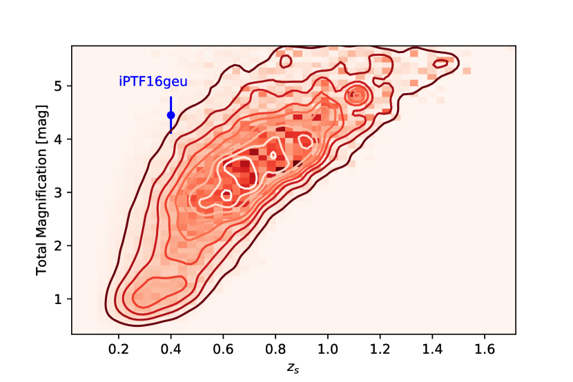
iPTF16geu (Goobar et al., 2017), the only gLSN Ia with resolved images discovered to date, is notable for its remarkably high magnification. Accounting for extinction, its four supernova images had a total magnification , significantly larger than the predicted (More et al., 2017). Amplification by unresolved lens galaxy stars (microlensing) was proposed as an explanation for this anomaly (More et al., 2017). In a subsequent investigation, Yahalomi et al. (2017) used microlensing ray-tracing simulations to show that microlensing alone could not account for the large observed flux anomalies. This may indicate that the anomaly is due to millilensing, but a systematic study of millilensing induced by lens-galaxy substructures on gLSNe has yet to be performed.
Thus the origin of the large magnification of iPTF16geu remains a mystery, but the simulations presented in this paper can help place this discrepancy in context. iPTF, the survey that found iPTF16geu, used the same telescope as ZTF (the P48), to observe the same region of sky to roughly the same depth, but at a lower cadence. Thus the ZTF results presented here should be quite similar to those for iPTF. Figure 40 shows the joint distribution of and for gLSNe Ia discovered in ZTF, showing that iPTF16geu is significantly more magnified than expected for its redshift . Was iPTF16geu a remarkable fluke, or is there fundamental physics at play that our models for lensing do not capture? Searches for new strongly lensed SNe with ZTF will likely resolve this intriguing question.
5 Conclusion
In this article, we have presented detailed simulations of the gLSN population and made predictions of the properties and rates of gLSNe that forthcoming synoptic time-domain imaging surveys will find. ZTF should discover roughly 20 gLSNe over the course of a three-year survey, and LSST should find roughly 3,500 over its 10-year lifetime. Most host galaxies will be multiply imaged, enabling detailed lens modeling if sufficiently deep high-resolution imaging is obtained. ZTF and LSST are sensitive to different gLSN populations. ZTF is most sensitive to compact, highly magnified quads with short time delays, whereas LSST is more sensitive to fainter doubles, which in general are less magnified and have longer delays. This will give LSST an advantage for time-delay cosmology if it can obtain the follow-up resources needed to extract spectroscopy and time delays from these transients. Our inclusion of dust decreases the expected gLSN Ia rate over the predictions of Goldstein et al. (2018), which did not include dust, by a factor of 2, but the predictions remain largely consistent with those of Goldstein & Nugent (2017). This study has found that gLSNe IIn will be the most frequently discovered by both ZTF and LSST. With respect to LSST observing strategy, we find that strategies that produce dense light curves at the expense of a larger survey area can yield comparable numbers of gLSNe, but the better-sampled surveys discover these gLSNe earlier and produce higher-quality light curves.
References
- Amanullah et al. (2015) Amanullah, R., Johansson, J., Goobar, A., et al. 2015, MNRAS, 453, 3300
- Arcavi et al. (2010) Arcavi, I., Gal-Yam, A., Kasliwal, M. M., et al. 2010, ApJ, 721, 777
- Bernardi et al. (2003) Bernardi, M., Sheth, R. K., Annis, J., et al. 2003, AJ, 125, 1866
- Bertin & Arnouts (1996) Bertin, E., & Arnouts, S. 1996, A&AS, 117, 393
- Bezanson et al. (2011) Bezanson, R., van Dokkum, P. G., Franx, M., et al. 2011, ApJ, 737, L31
- Birrer et al. (2018) Birrer, S., Treu, T., Rusu, C. E., et al. 2018, ArXiv e-prints, arXiv:1809.01274
- Bonvin et al. (2017) Bonvin, V., Courbin, F., Suyu, S. H., et al. 2017, MNRAS, 465, 4914
- Bridle et al. (2009) Bridle, S., Shawe-Taylor, J., Amara, A., et al. 2009, Annals of Applied Statistics, 3, 6
- Bulla et al. (2018) Bulla, M., Goobar, A., & Dhawan, S. 2018, MNRAS, 479, 3663
- Cardelli et al. (1989) Cardelli, J. A., Clayton, G. C., & Mathis, J. S. 1989, ApJ, 345, 245
- Chae (2003) Chae, K.-H. 2003, MNRAS, 346, 746
- Chae (2007) —. 2007, ApJ, 658, L71
- Choi et al. (2007) Choi, Y.-Y., Park, C., & Vogeley, M. S. 2007, ApJ, 658, 884
- Collett (2015) Collett, T. E. 2015, ApJ, 811, 20
- Collett & Cunnington (2016) Collett, T. E., & Cunnington, S. D. 2016, MNRAS, 462, 3255
- Delgado et al. (2014) Delgado, F., Saha, A., Chandrasekharan, S., et al. 2014, in Proc. SPIE, Vol. 9150, Modeling, Systems Engineering, and Project Management for Astronomy VI, 915015
- Djorgovski & Davis (1987) Djorgovski, S., & Davis, M. 1987, ApJ, 313, 59
- Dobler & Keeton (2006) Dobler, G., & Keeton, C. R. 2006, ApJ, 653, 1391
- Einstein (1936) Einstein, A. 1936, Science, 84, 506
- Foxley-Marrable et al. (2018) Foxley-Marrable, M., Collett, T. E., Vernardos, G., Goldstein, D. A., & Bacon, D. 2018, ArXiv e-prints, arXiv:1802.07738
- Gilliland et al. (1999) Gilliland, R. L., Nugent, P. E., & Phillips, M. M. 1999, ApJ, 521, 30
- Goldstein & Nugent (2017) Goldstein, D. A., & Nugent, P. E. 2017, ApJ, 834, L5
- Goldstein et al. (2018) Goldstein, D. A., Nugent, P. E., Kasen, D. N., & Collett, T. E. 2018, ApJ, 855, 22
- Goldstein et al. (2015) Goldstein, D. A., D’Andrea, C. B., Fischer, J. A., et al. 2015, AJ, 150, 82
- Goobar et al. (2017) Goobar, A., Amanullah, R., Kulkarni, S. R., et al. 2017, Science, 356, 291
- Graham & Driver (2005) Graham, A. W., & Driver, S. P. 2005, PASA, 22, 118
- Griffith et al. (2012) Griffith, R. L., Cooper, M. C., Newman, J. A., et al. 2012, ApJS, 200, 9
- Grillo et al. (2018) Grillo, C., Rosati, P., Suyu, S. H., et al. 2018, ArXiv e-prints, arXiv:1802.01584
- Gupta et al. (2016) Gupta, R. R., Kuhlmann, S., Kovacs, E., et al. 2016, AJ, 152, 154
- Guy et al. (2007) Guy, J., Astier, P., Baumont, S., et al. 2007, A&A, 466, 11
- Hakobyan et al. (2012) Hakobyan, A. A., Adibekyan, V. Z., Aramyan, L. S., et al. 2012, A&A, 544, A81
- Han et al. (2010) Han, D.-H., Park, C., Choi, Y.-Y., & Park, M.-G. 2010, ApJ, 724, 502
- Hatano et al. (1998) Hatano, K., Branch, D., & Deaton, J. 1998, ApJ, 502, 177
- Häußler et al. (2011) Häußler, B., Barden, M., Bamford, S. P., & Rojas, A. 2011, in Astronomical Society of the Pacific Conference Series, Vol. 442, Astronomical Data Analysis Software and Systems XX, ed. I. N. Evans, A. Accomazzi, D. J. Mink, & A. H. Rots, 155
- Häußler et al. (2007) Häußler, B., McIntosh, D. H., Barden, M., et al. 2007, ApJS, 172, 615
- Holz (2001) Holz, D. E. 2001, ApJ, 556, L71
- Hsiao et al. (2007) Hsiao, E. Y., Conley, A., Howell, D. A., et al. 2007, ApJ, 663, 1187
- James & Roos (1975) James, F., & Roos, M. 1975, Computer Physics Communications, 10, 343
- Keeton et al. (1997) Keeton, C. R., Kochanek, C. S., & Seljak, U. 1997, ApJ, 482, 604
- Kelly & Kirshner (2012) Kelly, P. L., & Kirshner, R. P. 2012, ApJ, 759, 107
- Kelly et al. (2015a) Kelly, P. L., Rodney, S. A., Treu, T., et al. 2015a, Science, 347, 1123
- Kelly et al. (2015b) Kelly, P. L., Brammer, G., Selsing, J., et al. 2015b, ArXiv e-prints, arXiv:1512.09093
- Kinney et al. (1996) Kinney, A. L., Calzetti, D., Bohlin, R. C., et al. 1996, ApJ, 467, 38
- Kochanek (1991) Kochanek, C. S. 1991, ApJ, 373, 354
- Kolatt & Bartelmann (1998) Kolatt, T. S., & Bartelmann, M. 1998, MNRAS, 296, 763
- Koopmans et al. (2009) Koopmans, L. V. E., Bolton, A., Treu, T., et al. 2009, ApJ, 703, L51
- Kormann et al. (1994) Kormann, R., Schneider, P., & Bartelmann, M. 1994, A&A, 284, 285
- Lackner & Gunn (2012) Lackner, C. N., & Gunn, J. E. 2012, MNRAS, 421, 2277
- Law et al. (2009) Law, N. M., Kulkarni, S. R., Dekany, R. G., et al. 2009, PASP, 121, 1395
- Levan et al. (2005) Levan, A., Nugent, P., Fruchter, A., et al. 2005, ApJ, 624, 880
- Li et al. (2011) Li, W., Leaman, J., Chornock, R., et al. 2011, MNRAS, 412, 1441
- Linder et al. (1988) Linder, E. V., Schneider, P., & Wagoner, R. V. 1988, ApJ, 324, 786
- LSST Science Collaboration et al. (2009) LSST Science Collaboration, Abell, P. A., Allison, J., et al. 2009, ArXiv e-prints, arXiv:0912.0201
- LSST Science Collaborations et al. (2017) LSST Science Collaborations, Marshall, P., Anguita, T., et al. 2017, ArXiv e-prints, arXiv:1708.04058
- Maoz et al. (2014) Maoz, D., Mannucci, F., & Nelemans, G. 2014, ARA&A, 52, 107
- More et al. (2017) More, A., Suyu, S. H., Oguri, M., More, S., & Lee, C.-H. 2017, ApJ, 835, L25
- Nugent et al. (2002) Nugent, P., Kim, A., & Perlmutter, S. 2002, PASP, 114, 803
- Oguri (2010) Oguri, M. 2010, PASJ, 62, 1017
- Oguri & Marshall (2010) Oguri, M., & Marshall, P. J. 2010, MNRAS, 405, 2579
- Oguri et al. (2008) Oguri, M., Inada, N., Strauss, M. A., et al. 2008, AJ, 135, 512
- Peng et al. (2002) Peng, C. Y., Ho, L. C., Impey, C. D., & Rix, H.-W. 2002, AJ, 124, 266
- Petrushevska et al. (2016) Petrushevska, T., Amanullah, R., Goobar, A., et al. 2016, A&A, 594, A54
- Planck Collaboration et al. (2016) Planck Collaboration, Ade, P. A. R., Aghanim, N., et al. 2016, A&A, 594, A13
- Refsdal (1964a) Refsdal, S. 1964a, MNRAS, 128, 295
- Refsdal (1964b) —. 1964b, MNRAS, 128, 307
- Riess et al. (2018) Riess, A. G., Casertano, S., Yuan, W., et al. 2018, ArXiv e-prints, arXiv:1801.01120
- Rowe et al. (2015) Rowe, B. T. P., Jarvis, M., Mandelbaum, R., et al. 2015, Astronomy and Computing, 10, 121
- Sako et al. (2011) Sako, M., Bassett, B., Connolly, B., et al. 2011, ApJ, 738, 162
- Scalzo et al. (2014) Scalzo, R., Aldering, G., Antilogus, P., et al. 2014, MNRAS, 440, 1498
- Schlegel et al. (1998) Schlegel, D. J., Finkbeiner, D. P., & Davis, M. 1998, ApJ, 500, 525
- Schneider & Wagoner (1987) Schneider, P., & Wagoner, R. V. 1987, ApJ, 314, 154
- Scoville et al. (2007) Scoville, N., Aussel, H., Brusa, M., et al. 2007, ApJS, 172, 1
- Sérsic (1963) Sérsic, J. L. 1963, Boletin de la Asociacion Argentina de Astronomia La Plata Argentina, 6, 41
- Shen et al. (2003) Shen, S., Mo, H. J., White, S. D. M., et al. 2003, MNRAS, 343, 978
- Sheth et al. (2003) Sheth, R. K., Bernardi, M., Schechter, P. L., et al. 2003, ApJ, 594, 225
- Shu et al. (2018) Shu, Y., Bolton, A. S., Mao, S., et al. 2018, ArXiv e-prints, arXiv:1803.07569
- Smith et al. (2012) Smith, M., Nichol, R. C., Dilday, B., et al. 2012, ApJ, 755, 61
- Spergel et al. (2013) Spergel, D., Gehrels, N., Breckinridge, J., et al. 2013, ArXiv e-prints, arXiv:1305.5422
- Stritzinger et al. (2018) Stritzinger, M. D., Taddia, F., Burns, C. R., et al. 2018, A&A, 609, A135
- Sullivan et al. (2000) Sullivan, M., Ellis, R., Nugent, P., Smail, I., & Madau, P. 2000, MNRAS, 319, 549
- Sullivan et al. (2006) Sullivan, M., Le Borgne, D., Pritchet, C. J., et al. 2006, ApJ, 648, 868
- Suwa (2018) Suwa, Y. 2018, MNRAS, 474, 2612
- Suyu et al. (2017) Suyu, S. H., Bonvin, V., Courbin, F., et al. 2017, MNRAS, 468, 2590
- Vega-Ferrero et al. (2018) Vega-Ferrero, J., Diego, J. M., Miranda, V., & Bernstein, G. M. 2018, ApJ, 853, L31
- Witt & Mao (1997) Witt, H. J., & Mao, S. 1997, MNRAS, 291, 211
- Wong et al. (2011) Wong, K. C., Keeton, C. R., Williams, K. A., Momcheva, I. G., & Zabludoff, A. I. 2011, ApJ, 726, 84
- Yahalomi et al. (2017) Yahalomi, D. A., Schechter, P. L., & Wambsganss, J. 2017, ArXiv e-prints, arXiv:1711.07919
- Zwicky (1937) Zwicky, F. 1937, Physical Review, 51, 290