Internal and Collective Properties of Galaxies in the Sloan Digital Sky Survey

Abstract

We examine volume-limited samples of galaxies drawn from the Sloan Digital Sky Survey to look for relations among internal and collective physical parameters of galaxies as faint as $M_{r}=-17.5$. The internal physical properties of interest include morphology, luminosity, color, color gradient, concentration, size, velocity dispersion, equivalent width of $H{\alpha}$ line, and axis ratio. Collective properties that we measure include the luminosity and velocity dispersion functions. We morphologically classify galaxies using the three dimensional parameter space of $u-r$ color, $g-i$ color gradient, and concentration index. All relations are inspected separately for early and late type galaxies. At fixed morphology and luminosity, we find that bright ($M_{r}<-20$) early type galaxies show very small dispersions in color, color gradient, concentration, size, and velocity dispersion. These dispersions increase at fainter magnitudes, where the fraction of blue star-forming early types increases. Late types show wider dispersions in all physical parameters compared to early types at the same luminosity. Concentration indices of early types are well correlated with velocity dispersion, but are insensitive to luminosity and color for bright galaxies, in particular. The slope of the Faber-Jackson relation ($L\propto{\sigma}^{\gamma}$) continuously changes from $\gamma=4.6\pm 0.4$ to $2.7\pm 0.2$ when luminosity changes from $M_{r}=-22$ to $-20$. The size of early types is well-correlated with stellar velocity dispersion, $\sigma$, when $\sigma>100$ km s^-1. We find that passive spiral galaxies are well separated from star-forming late type galaxies at $H{\alpha}$ equivalent width of about 4. An interesting finding is that many physical parameters of galaxies manifest different behaviors across the absolute magnitude of about $M_{\rm\ast}\pm 1$. The morphology fraction as a function of luminosity depends less sensitively on large-scale structure than the luminosity function (LF) does, and thus seems to be more universal. The effects of internal extinction in late type galaxies on the completeness of volume-limited samples and on the LF and morphology fraction are found to be very important. An important improvement of our analyses over most previous works is that the extinction effects are effectively reduced by excluding the inclined late type galaxies with axis ratios of $b/a<0.6$.

1. Introduction

With the large and homogeneous redshift surveys like the Sloan Digital Sky Survey (SDSS; York et al.2000) and Two Degree Field Galaxy Redshift Survey (2dFGRS; Colless et al. 2001), our view of the local universe became extended out to a few hundred mega parsecs. From such dense redshift surveys, the small-scale distribution of galaxies is also being revealed in more detail. It is now possible to make very accurate measurements of various relations among the physical properties of galaxies and the local environment. This is a difficult task, which should be completed before theoretical modeling and interpretations are attempted. The study is complicated because there are many physical parameters involved and their mutual relations are non-trivially interrelated. A further complication is the fact that definition of environment depends on the type of objects chosen to trace the large scale-structure.

One could divide the physical properties of galaxies into internal and collective ones. Examples of internal physical properties are color, luminosity, morphology, star formation rate, velocity dispersion, surface brightness, spectral type, size, and so on. Collective properties can be the strength and statistical nature of spatial clustering, peculiar velocity field, luminosity function, velocity dispersion distribution function, halo mass function, axis ratio distribution function and so on (see Fig. 1).

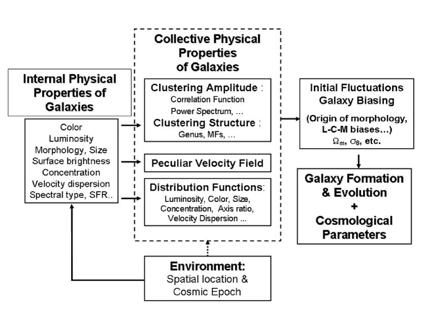
Figure 1.— Schematic diagram showing some key science for understanding the structure formation and the background universe.

On the other hand, the local environments can be spatial or temporal. Dependence on the latter means the evolution in cosmic time. ”Spatial environment” can have various meanings. Traditionally discrete types, such as cluster, group, field, or void, are used to distinguish among different environments of galaxies. Recently, the smoothed number density of neighboring galaxies was also used to represent the environment. One could also use other parameters to define the environment of galaxies. Density gradient, shear fields, and large-scale peculiar velocity fields can be important parameters affecting the properties of galaxies. The relations among all these physical observables and environment can give us information on galaxy formation and the background universe. Many authors in the past have investigated the relations between environment and galaxy properties (Lewis et al. 2002; Gómez et al. 2003; Goto et al. 2003a; Balogh et al. 2004a, 2004b; Hogg et al. 2004; Tanaka et al. 2004; Kuehn & Ryden 2005; Desroches et al. 2006).

There has been much recent progress in studying the correlation between the distribution of galaxies and their basic properties, and the correlation among the properties. For example, the luminosity function of galaxies subdivided by various criteria has been measured. Blanton et al. (2003a) presented the luminosity functions of the SDSS galaxies defined by galaxy light profile shape. Madgwick et al. (2002) measured the luminosity function of 2dFGRS for different type of galaxies defined by their spectral properties. Nakamura et al. (2003) studied the dependence of the luminosity function on galaxy morphology and the correlation between galaxy morphology and other photometric properties such as color and concentration index using a sample of SDSS galaxies with visually identified morphological types. Weinmann et al. (2006) performed an extensive study of the dependence of color, star formation, and morphology of galaxies on halo mass using galaxy groups selected in the SDSS DR2. Shen et al. (2003) examined the correlation between the size distribution of galaxies and other properties such as their luminosity, stellar mass and morphological type. Baldry et al. (2004) analyzed the bivariate distribution of the SDSS galaxies in the color versus absolute magnitude space. The fundamental plane and the color-magnitude-velocity dispersion relation for early type galaxies with SDSS have been investigated by Bernardi et al. (2003a, 2005) Very recently Desroches et al. (2006) showed that the fundamental plane projections of elliptical galaxies depend on luminosity using DR4 of the SDSS. In particular, they found that the radius-luminosity and Faber-Jackson relations are steeper at high luminosity, which we also found in our work using a larger SDSS sample with morphologically cleaner early type samples. Sheth et al. (2003) and Mitchell et al. (2005) measured the velocity dispersion distribution function of early type galaxies carefully selected from the SDSS samples using selection criteria similar to those of Bernardi et al. (2003a). Alam & Ryden (2002) measured the axis ratio distributions for red and blue galaxies fitted by the de Vaucouleurs and exponential profiles.

This paper focuses on understanding of the relationship among many physical properties of galaxies using a set of volume-limited samples of the SDSS galaxies, which are further divided into subsamples of constant morphology and absolute magnitude. This well-controlled experiment allows us to measure the relations among internal and collective properties as a function of morphology and luminosity. In our companion paper we have studied the dependence of various galaxy properties on the local density environment (Park et al. 2006, hereafter Paper II).

This paper is organized as follows. In section 2, we describe our catalog and morphology classification and the physical parameters that we use in Section 3 and 4 to investigate the relations among the galaxy properties. We summarize our results in Section 5.

2. Observational Data Set

2.1. Sloan Digital Sky Survey

The SDSS (York et al. 2000; Stoughton et al. 2002; Adelman-McCarthy et al. 2006) is a survey to explore the large-scale distribution of galaxies and quasars by using a dedicated $2.5{\rm m}$ telescope at Apache Point Observatory (Gunn et al. 2006). The photometric survey has imaged roughly $\pi$ sr of the northern Galactic cap in five photometric bandpasses denoted by $u$, $g$, $r$, $i$, and $z$ centered at $3551,4686,6165,7481,$ and $8931\AA$, respectively, by an imaging camera with 54 CCDs (Fukugita et al. 1996; Gunn et al. 1998). The limiting magnitudes of photometry at a signal-to-noise ratio of $5:1$ are $22.0,22.2,22.2,21.3$, and $20.5$ in the five bandpasses, respectively. The median width of the point-spread function (PSF) is typically $1.4\arcsec$, and the photometric uncertainties are $2\%$ rms (Abazajian et al. 2004).

After image processing (Lupton et al. 2001; Stoughton et al. 2002; Pier et al. 2003) and calibration (Hogg et al. 2001; Smith et al. 2002; Ivezić et al. 2004; Tucker et al. 2006), targets are selected for spectroscopic follow-up observation. The spectroscopic survey is planned to continue through 2008 as the Legacy Survey and to yield about $10^{6}$ galaxy spectra. The spectra are obtained by two dual fiber-fed CCD spectrographs. The spectral resolution is $\lambda/\Delta\lambda\sim 1800$, and the rms uncertainty in redshift is $\sim 30$ km s^-1. Because of the mechanical constraint of using fibers, no two fibers can be placed closer than $55\arcsec$ on the same tile. Mainly due to this fiber collision constraint, incompleteness of spectroscopy survey reaches about 6% (Blanton et al. 2003b) in such a way that regions with high surface densities of galaxies become less prominent even after adaptive overlapping of multiple tiles. This angular variation of sampling density is accounted for in our analysis.

The SDSS spectroscopy yields three major samples: the main galaxy sample, the luminous red galaxy sample (Eisenstein et al. 2001), and the quasar sample (Richards et al. 2002). The main galaxy sample is a magnitude-limited sample with an apparent Petrosian $r$-magnitude cut of $m_{r,\mathrm{lim}}\approx 17.77$, which is the limiting magnitude for spectroscopy (Strauss et al. 2002). It has a further cut in Petrosian half-light surface brightness $\mu_{R50},\mathrm{lim}=24.5$ mag/arcsec². More details about the survey can be found on the SDSS web site.

In our study of galaxy properties, we use a subsample of SDSS galaxies known as the New York University Value-Added Galaxy Catalog (NYU-VAGC; Blanton et al 2005). This sample is a subset of the recent SDSS Data Release 5. One of the products of the NYU-VAGC used here is a large-scale structure sample DR4plus (LSS-DR4plus). For local density estimation in the three-dimensional redshift space in our accompanying paper we use galaxies within the boundaries shown in Figure 1 of Paper II, which improves the volume-to-surface area ratio of the survey. There are also three stripes in the southern Galactic cap observed by SDSS. Density estimation is difficult within these narrow stripes, so for consistency with the samples examined in the accompanying paper, we do not use them. The remaining survey region covers $4464$ deg². The primary sample of galaxies used here is a subset of the LSS-DR4plus sample referred to as ”void0”, which is further selected to have apparent magnitudes in the range $14.5<r<17.6$ and redshifts in the range $0.001<z<0.5$. These cuts yield a sample of 312,338 galaxies. The roughly 6% of targeted galaxies that do not have a measured redshift due to fiber collisions are assigned the redshift of their nearest neighbor.

Completeness of the SDSS is poor for bright galaxies with $r<14.5$ because of both the spectroscopic selection criteria (which excludes objects with large flux within the 3$\arcsec$ fiber aperture; the cut at $r=14.5$ is an empirical approximation of the completeness limit caused by that cut) and the difficulty of obtaining correct photometry for objects with large angular size. For these reasons, analysis of SDSS galaxy samples have typically been limited to $r>14.5$. This is unfortunate because it limits the range of luminosity that can be probed; using the magnitude limits of the void0 sample the range of absolute magnitude is only about 3.1 at a given redshift. To extend the range of magnitude, we attempt to complete the redshift sample by supplementing the catalog with redshifts of bright galaxies, first from SDSS itself, and then by matching to earlier redshift catalogs (the missing galaxies are quite bright and easily observed by earlier surveys). We employ another subset of the LSS-DR4plus sample referred as bvoid, which is made before redshift determination and includes galaxies with $r<14.5$. Galaxies in bvoid with SDSS redshifts are added to the catalog. For those objects lacking redshifts, we searched earlier catalogs. Out of $5227$ bright objects with $r<14.5$ in the bvoid sample and within our survey region, we assign redshifts to 3945 galaxies cross matched with the Updated Zwicky Catalog (UZC; Falco et al. 1999), 807 galaxies from the bvoid sample after redshift determination, 69 galaxies from the Center for Astrophysics (CfA) redshift catalog (ZCAT 2000 Version), and 4 galaxies from the IRAS Point Source Catalog Redshift Survey (Saunders et al. 2000). We found 336 bright objects to be errors, such as outlying parts of a large galaxies that were deblended by the automated photometric pipeline, blank fields, stars, etc. Out of the remaining 66 objects, 30 galaxies are included in our sample, using redshifts from the NASA Extragalactic Database (NED). Only 36 galaxies remain in the bright bvoid sample with no measured redshift. In addition to these bright bvoid galaxies, which have been selected based on their $r$-band magnitudes, we have included the redshifts of 340 UZC galaxies cross-matched with SDSS objects in NYU-VAGC, which were not included in the previous step. Out of 6295 UZC galaxies within our survey region, 242 are still not matched with SDSS objects in the NYU-VAGC. Ofthe missing UZC galaxies, 60% have redshifts smaller than our inner redshift cut of $z=0.025$, leaving only 99 galaxies missing at larger redshift.

In total, we add 5195 bright ($r<14.5$) galaxies to the void0 samples, which yields a final sample of 317533 galaxies. Volume-limited samples derived from the resulting catalog have nearly constant comoving number density of galaxies along the radial direction at redshift $z\geq 0.025$. Thus, we treat our final samples as having no bright limit at redshift greater than $z=0.025$.

2.2. Definitions for the Volume-limited Samples

In this study we use only volume-limited samples of galaxies selected by absolute magnitude and redshift limits. Figure 2 shows the definitions of our six subsamples in redshift-absolute magnitude space.

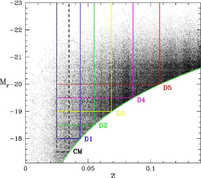
Figure 2.— Sample definitions of our six volume-limited SDSS samples in redshift vs. absolute magnitude space.

The shallowest subsample is labeled CM, which stands for ‘color-magnitude’. We employ the CM sample to extend some of our analyses to fainter absolute magnitude. The deeper and thicker (along the line of sight) five samples, from D1 to D5, are the main samples for study of galaxy properties. The definitions for all samples are summarized in Table 1.

Table 1Volume-limited Samples

Name	Absolute Magnitude	Redshift	Distance	Galaxies$(N_{E}\tablenotemark{b})$	$\bar{d}$
CM	$-17.5>M_{\rm r}$	$0.025<z<0.03484$	$74.6<R<103.7$	11756 (3467)	3.00
D1	$-18.0>M_{\rm r}$	$0.025<z<0.04374$	$74.6<R<129.9$	20288 (6256)	3.41
D2	$-18.5>M_{\rm r}$	$0.025<z<0.05485$	$74.6<R<162.6$	32550 (11341)	3.78
D3	$-19.0>M_{\rm r}$	$0.025<z<0.06869$	$74.6<R<203.0$	49571 (19270)	4.18
D4	$-19.5>M_{\rm r}$	$0.025<z<0.08588$	$74.6<R<252.9$	74688 (33039)	4.58
D5	$-20.0>M_{\rm r}$	$0.025<z<0.10713$	$74.6<R<314.0$	80479 (39333)	5.56

The comoving distance and redshift limits of each volume-limited sample defined by an absolute magnitude limit are obtained by using the formula

$$m_{r,{\rm lim}}-M_{r,{\rm lim}}=5{\rm log}(r(1+z))+25+\bar{K}(z)+\bar{E}(z),$$ (1)

where $\bar{K}(z)$ is the mean $K$-correction, $\bar{E}(z)$ is the mean luminosity evolution correction, and $r$ is the comoving distance corresponding to redshift $z$. We adopt a flat $\Lambda$CDM cosmology with density parameters $\Omega_{\Lambda}=0.73$ and $\Omega_{m}=0.27$ to convert redshift to comoving distance. To determine sample boundaries we use a polynomial fit to the mean $K$-correction,

$$\bar{K}(z)=3.0084(z-0.1){{}^{2}}+1.0543(z-0.1)-2.5{\rm log}(1+0.1).$$ (2)

We apply the mean luminosity evolution correction given by Tegmark et al. (2004), $E(z)=1.6(z-0.1)$. The rest-frame absolute magnitudes of individual galaxies are computed in fixed bandpasses, shifted to $z=0.1$, using Galactic reddening corrections (Schlegel et al. 1998) and $K$-corrections as described by Blanton et al. (2003c). This means that a galaxy at $z=0.1$ has a $K$-correction of $-2.5{\rm log}(1+0.1)$, independent of its spectral energy distribution (SED). We have applied the same mean luminosity evolution correction formula to individual galaxies.

2.3. Physical Parameters of Galaxies

The physical parameters we consider in this study are ${}^{0.1}(u-r)$ color, absolute Petrosian magnitude in the $r$-band $M_{r}$, morphology (see below), Petrosian radius, axis ratio, concentration index, color gradient in ${}^{0.1}(g-i)$ color, velocity dispersion, and equivalent width of the H$\alpha$ line.

To compute colors, we use extinction and $K$-corrected model magnitudes. The superscript 0.1 means the rest-frame magnitude $K$-corrected to the redshift of 0.1. All our magnitudes and colors follow this convention, and the superscript will subsequently be dropped. To measure some of the physical parameters of galaxies, we retrieve the $g$- and $i$-band atlas images and basic photometric parameters of all galaxies in our sample from the archive of photometric reductions conducted by the Princeton/NYU group. To take into account flattening or inclination of galaxies, we use elliptical annuli in all parameter calculations, and the isophotal position angle and axis ratio in the $i$-band are used to define the elliptical annuli. The $g-i$ color gradient is defined to be the color difference between the region with $R<0.5R_{\rm Pet}$ and the annulus with $0.5R_{\rm Pet}<R<R_{\rm Pet}$, where $R_{\rm Pet}$ is the Petrosian radius. The (inverse) concentration index is defined by $R_{50}/R_{90}$ where $R_{50}$ and $R_{90}$ are the semi-major axis lengths of ellipses containing 50% and 90% of the Petrosian flux in the $i$-band image, respectively. The $g-i$ color gradient, concentration index, and isophotal axis ratios are corrected for the effects of seeing. To do so, we first generate a large set of Sersic model images with various scaling lengths, slopes, and axis ratios convolved with a range of PSF sizes. For an observed galaxy image with a given size of the PSF we look for a best-fit Sersic model when the Sersic model is convolved with the PSF to find the true Sersic index and the true axis ratio. The fit is made at radii between $0.2$ and $1.0R_{\rm Pet}$ to avoid the central region, whose profile is strongly affected by seeing. When the best-fit Sersic models are found in the $g$ and $i$ bands, the $g-i$ color gradient and concentration index are calculated for the true Sersic models and their differences from those of convolved images are used to correct the color gradient of the observed image for the seeing effects.

We classify galaxy morphologies into early (ellipticals and lenticulars) and late (spirals and irregulars) types using the automated galaxy morphological classification method given by Park & Choi (2005), who showed that incorporating the $g-i$ color gradient into the classification parameter space allows us to successfully separate the two populations degenerated in $u-r$ color and the concentration index helps us separate red disky spirals from early type galaxies (see Fig. 1 of Park & Choi 2005). It should be noted that the “morphological” properties of galaxies can change when different bands are adopted. The difference in morphology in different bands is exactly the color distribution, which is reflected in our color gradient parameter. To define the classification boundaries in this multi-parameter space, they used a training set of 1982 SDSS galaxies whose morphological types are visually identified. The distributions of the early and late type galaxies in sample D2 are shown in Figures 6$a$ and 6$b$, below. The reader is referred to Park & Choi (2005) for further details of the methods and various tests. We have visually examined color images of a set of faint galaxies retrieved by the SDSS Image List, and confirmed that the resulting morphological classification is highly successful with completeness and reliability reaching 90%. For the volume-limited samples D2 and CM we made an additional visual check to correct possible misclassifications of the automated scheme for blue early types (those below the straight line in Fig. 3$a$) and red late types (those redder than $2.4$ in $u-r$ color). The morphological types of 1.9% of galaxies, which are often blended or merged objects, were changed by this procedure. This morphology classification allows us to make very accurate measurements in this study compared with previous work. We discuss this further in section 3.2.

3. Relations Among Physical Parameters of Galaxies

We find that absolute magnitude and morphology are the most important parameters characterizing physical properties of galaxies, in the sense that other parameters show relatively little scatter once absolute magnitude and morphology are fixed. This is particularly true for early type galaxies. We begin this section by showing the dependence of various physical parameters of galaxies on their absolute magnitudes. In each case, we separately examine samples of early (E/S0) and late (S/Irr) morphological types.

3.1. Variation with Absolute Magnitude

Figure 3$a$ shows the color-absolute magnitude diagram of galaxies in the CM and D2 samples.

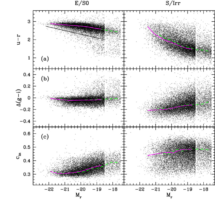
Figure 3.— Relations between the absolute magnitude and ($a$) $u-r$ color, ($b$) $\Delta(g-i)$ color gradient, and (c) $c_{\rm in}$ (inverse) concentration index of galaxies in the D2 (brighter than $M_{r}=-18.5$) and CM (fainter than $-18.45$) volume-limited subsamples of the SDSS. E/S0 morphological types are shown in the left panels, and S/Irr types are shown in the right panels. Curves delineate the locations of the most probable parameter values as a function of absolute magnitude. The solid curve is for the D2 sample, and the dashed curve is for the CM sample.

Galaxies in the CM sample are shown only for $-17.5>M_{r}>-18.45$. The left panel shows the distribution of early types, and the right panel shows that of late types. The solid and dashed lines delineate the most probable $u-r$ color of galaxies in the D2 and CM samples, respectively. (Here and throughout, the “most probable” parameter value within 0.4 absolute magnitude bin is the mode of the distribution of that parameter.) The most probable color of the red sequence galaxies has a break at $M_{r}\approx-19.6$ and has slopes of about $-0.07$ at the bright side and about $-0.15$ at the faint side. We plot only those late type galaxies with axis ratios $b/a>0.6$, to reduce the biases in absolute magnitude, color, color gradient, etc., due to internal extinction. Colors of late types have a much wider dispersion. Their most probable color rapidly becomes bluer as galaxies become fainter, but is very insensitive to absolute magnitude fainter than $M_{r}=-18$, approaching $u-r\approx 1.1$ at the very faint end ($M_{r}\sim-14$, not shown).

Baldry et al. (2004) reported a slope of about $-0.08$ for luminous red galaxies selected from the SDSS, which is consistent with our measurement. One significant difference between Baldry et al.’s and our result is the color-magnitude relation of the late type (blue distribution) galaxies at the bright side. In their results the slope of the relation becomes less steep long before the color-magnitude relation for late types touches that of early types as one, toward brightest magnitude. On the other hand, our result shows no such bending until it approaches the relation for early types. The difference is probably caused by extinction of late type galaxies.

Figure 3$a$ shows that the color distribution of late type galaxies overlaps with early types at all magnitudes, and vice versa. The solid straight line in Figure 3$a$ roughly divides the sequences of red and blue galaxies. However, about 24% of spiral/irregular galaxies brighter than $M_{r}=-18.5$ are above this line when all inclinations are allowed. Among all galaxies above this line, 32% are actually late types. Therefore, an early type sample generated by a simple cut in the absolute magnitude versus color space must take into account this huge contamination. We also find a significant fraction of early types located outside the main red sequence at faint magnitudes. At absolute magnitudes between $-18.5$ and $-19.0$, about 10% of early types are located below the straight line shown in Figure 3$a$. This outlying fraction is larger at fainter magnitudes. Some of these blue early type galaxies may be actually spirals whose disks look too faint for both our automated and visual classification schemes to classify correctly, but the trend seems robust.

Again, it should be noted that even though the bimodality in galaxy color is mainly due to the bimodality in galaxy morphology, there is a significant overlap in color space between the two morphological classes. With few exceptions, very blue ($u-r<1.8$) early type galaxies show strong emission lines in their spectra, indicating active star formation (see Fig. 6$c$). The distributions of colors of early and late types at a given absolute magnitude are not Gaussian. The colors of early types are skewed to blue color, and those of late types are skewed to red color. The blue sequence appears less prominent when the data is contaminated by internal extinction effects (see Fig. 12, below).

Figure 3$b$ shows distributions of galaxies in color gradient, $\Delta(g-i)$, versus absolute magnitude, $M_{r}$. We find that the majority of E/S0’s (left panel) have a weak negative color gradient; the envelope is slightly bluer than the core. Their most probable color gradient is surprisingly constant at $\Delta(g-i)=-0.035\pm 0.007$ at all magnitudes explored, with a weak trend for more positive gradient toward faint and bright magnitudes. Interestingly, the E/S0’s with $M_{r}\approx M_{\ast}-0.5$ have the minimum color gradient. It should be noted that the color gradient of the brightest early types approaches zero, meaning that the brightest early types are reddest and most spatially homogeneous in color. Although the most probable color gradient has a nearly constant of absolute magnitude, the number of E/S0’s with blue cores increases strongly at absolute magnitudes fainter than $M_{*}$.

The color gradient of late type galaxies is more negative (i.e., bluer envelope) than that of early types and is a slowly increasing function of absolute magnitude Faint late types are more gas rich and have more uniform internal star formation activity, while bright late types have red central bulges and blue star forming disk structures.

Figure 3$c$ shows that the (inverse) concentration index $c_{\rm in}$ of the early types (left panel) is nearly independent of absolute magnitude when $M_{r}<M_{*}$, but rises rather steeply at fainter magnitudes. The most probable concentration index of the bright early types is close to that of a de Vaucouleurs profile ($c_{\rm in}=0.29$), even though it slightly increases at the brightest end. The brightest early types might be less concentrated because of more recent mergers, and the galaxies only slightly brighter than $M_{\ast}$, with $M_{r}\sim M_{\ast}-0.9$ might be dynamically older (more relaxed). For late type galaxies the most probable value is close to the value an exponential disk ($c_{\rm in}=0.44$) at the brightest end, albeit with a large dispersion.

The Petrosian radius in units of $h^{-1}$ kpc as a function of absolute magnitude is shown in Figure 4$a$. The Petrosian radius is calculated by using the elliptical annuli, and is typically larger than the value in the SDSS Photometric database which uses the circular annuli. Early type galaxies (left panel) exhibit a tight correlation between physical size and luminosity, and the relation has a significant curvature. The slope is very steep ($d{\rm log}R_{\rm Pet}/dM_{r}\approx-0.28$ at $M_{r}\approx-21.5$) at the brightest end. The late types have larger $R_{\rm Pet}$, and their size relation with absolute magnitude is less curved. The curvature of the relation for both early and late types means that fainter galaxies have lower surface brightness. As a guide the radius-magnitude relation in the case of constant surface brightness ($L\propto\Sigma R^{2}$ where $L$ is luminosity and $\Sigma$ is surface brightness) is drawn in both panels. The slope of this relation to the bright end of the late types tells that the brightest spiral galaxies, with $M_{r}\leq-21$, have surface brightness approximately independent of luminosity. This relation is also true for the early types in the regime $-21\leq M_{r}\leq-20$ fainter than for the late types. Desroches et al. (2006) also found that the radius-luminosity relation of elliptical galaxies is steeper at high luminosity. Shen et al. (2003) measured the size distributions of early and late type galaxies, divided by the concentration index or the Sersic index, and found that they are well fitted by a log normal distribution.

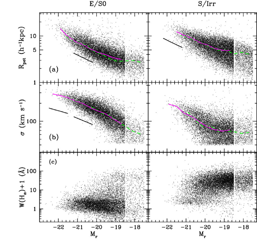
Figure 4.— Relations between the absolute magnitude and ($a$) the Petrosian radius, ($b$) velocity dispersion, and ($c$) equivalent width of the $H{\alpha}$ line of galaxies in the D2 (brighter than $M_{r}=-18.5$) and CM (fainter than $-18.45$) volume-limited subsamples of the SDSS survey. E/S0 morphological types are shown in the left panels, and S/Irr types are shown in the right panels. Curves have the same meanings as in Fig. $3a-3c$.

Figure 4$b$ shows the variation with absolute magnitude of velocity dispersion, as measured by an automated spectroscopic pipeline called IDLSPEC2D version 5 (D. Schlegel et al. 2007, in preparation). Galaxy spectra of the SDSS are obtained by optical fibers with radius of $R_{\rm fib}=1.5\arcsec$. The finite size of this aperture smooths the central velocity dispersion profile. To correct the central velocity dispersion for this smoothing effects we adopt a simple aperture correction, $\sigma_{\rm corr}=\sigma_{\rm fib}(8R_{\rm fib}/R_{0})^{0.04}$ (Jørgensen et al. 1995; Bernardi et al. 2003b), where $R_{0}$ is the equivalent circular effective radius $(b/a)^{1/2}_{\rm deV}r_{\rm deV}$ where $r_{\rm deV}$ is the seeing-corrected effective angular radius along major axis of the galaxy from model fits to a de Vaucouleurs profile in the $i$ band. Because the measured velocity dispersion is systematically affected by the finite resolution of the spectrographs at small values, the calculation of the most probable velocity dispersion is restricted to galaxies with $\sigma>40$ km s^-1. The errors in the measured velocity dispersions are about $\sim 15\%$ at 70 km s^-1 and $\sim 30\%$ at 50 km s^-1. The dispersion in $\sigma$ is typically $\Delta{\rm log}\sigma=0.11$, and the measurement error is typically 11 km s^-1 (see section 4.2). From these data we fit the slope, $\gamma$, defined by $L\approx\sigma^{\gamma}$. At the bright end, near absolute magnitude $M_{r}=-22$, we find $\gamma=4.6\pm 0.4$, while the slope at magnitudes between $M_{r}=-21$ and $-20$ drops to $\gamma=2.7\pm 0.2$ (All five volume-limited samples are used for the measurements). For comparison, we plot two straight lines with slopes of $\gamma=4$ (upper left, Fig. 4$b$) and 3 (lower right, Fig. 4$b$), the former being the slope of the Faber-Jackson relation. Recently, Desroches et al. (2006) also found that the slope $\gamma$ is steeper at high luminosity, which is consistent with our findings. The measured velocity dispersion of spiral galaxies brighter than $M_{r}=-20.5$ is $70\%\pm 2$% of that of early types (or $\sigma_{\rm late}\approx\sigma_{\rm early}/\sqrt{2}$) at a given absolute magnitude.

Because SDSS fiber spectra sample the light from only the central $1.5\arcsec$ radius region of galaxies, the measured spectral parameters are not fully representative of the physical properties of spiral galaxies, which tend to have large variation of star formation activity from the bulge to outer disk. Nevertheless, parameters based on fiber spectra, such as line widths and those from the principal component analysis, are often used to characterize the star formation activity, morphological types, etc. (e.g. Tanaka et al. 2004; Balogh et al. 2004b). Thus, for comparison, we show such results for our samples.

The right panel of Figure 4$c$ shows the equivalent width of the $H\alpha$ line of late types as a function of $M_{r}$. The equivalent width of the $H{\alpha}$ line is often used as a measure of recent star formation activity (or nuclear activity). The majority of late types have large $W(H\alpha)$. The plot shows that fainter galaxies tend to have larger $W(H\alpha)$. This result should be considered carefully because the fiber spectra systematically miss the light from the outer disks of bright large galaxies, which might be active in star formation. The figure also shows that there is a class of late types that have weak $H\alpha$ line emission. The placement in this diagram of some of these objects may be due to the finite fiber size, but some of them are genuine passive spirals (Couch et al. 1998; Poggianti et al. 1999; Goto et al. 2003b; Yamauchi & Goto 2004).

The left panel of Figure 4$c$ shows $W(H\alpha)$ of early type galaxies. We find that the number of early types with central star formation activity increases sharply at absolute magnitudes fainter than $\sim M_{\ast}$. We find similar trends for $u-r$ color and $\Delta(g-i)$ color gradient (see also Fig. 6, below). Early types with central star formation activities have been studied and some of them are $\rm{E+A}$ galaxies (Goto et al. 2003c; Fukugita et al. 2004; Quintero et al. 2004; Goto 2005; Park & Choi 2005; Yamauchi & Goto 2005).

Figure 5 shows the isophotal axis ratio of early (left panel) and late (right panel) types as a function of absolute magnitude.

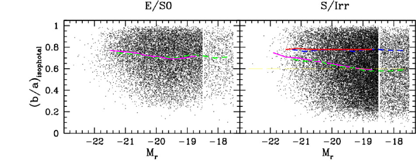
Figure 5.— Isophotal axis ratios of the early (left) and late (right) type galaxies in sample D2 (solid magenta line) and CM (dashed green line). Curves are the median values. For late types we added the median curves, in red and blue colors, derived from only those with $b/a>0.6$.

We choose the isophotal axis-ratio rather than axis ratios from de Vaucouleurs or exponential profile fits that are computed by the automated SDSS pipeline in our study because the isophotal position angles correspond most accurately to the true orientation of the major axis. The exponential profile fit is often bad particularly for barred spiral galaxies. Curves in Figure 5 are the median axis ratios of galaxies in the D2 (solid line) and CM (dashed line) samples. We also draw the median curves in red and blue colors by using only galaxies with $b/a>0.6$.

We clearly see that early type galaxies tend to be rounder at brighter magnitudes. Figure 5 demonstrates that the absolute magnitudes of inclined late types with $b/a<0.6$ seriously suffer from dimming due to the internal absorption, while the effects are ignorable for those with $b/a>0.6$. See also Figure 12, below and discussion in section 4.3.

3.2. Variation with Color

Figure 6$a$ shows the distribution of E/S0 (left panel) and S/Irr (right panel) galaxies in the D2 sample in the $u-r$ color versus $\Delta(g-i)$ color gradient space. Our morphological classification is based primarily on this parameter space. Note that the sharp boundaries shown in Figure 6a are due to a choice of our morphological criteria in the $u-r$ versus $g-i$ color gradient space, which is determined to correlate well with visually classified morphologies. Scatter across the classification boundaries is caused by the concentration index constraint on early types (see Park & Choi 2005 for details) and corrections made by visual inspection. Most early type galaxies fall within a strong concentration near $u-r=2.8$ and $\Delta(g-i)=-0.04$ in this plane. Because the color of the red sequence becomes bluer at fainter magnitudes (see Figure 3a), the center of this concentration moves to bluer $u-r$ when one examines fainter early types. There is also a trail of early types towards bluer colors and more positive color gradients. The classification boundary separating this blue early types from late types has been determined from a training set that showed such a trend (Park & Choi 2005). The majority of galaxies in this early type trail are fainter than $M_{\ast}$ (blue points), often show emission lines (see early types in Fig. 6$c$), and live mainly at intermediate and low density environments (see early types in Fig. 11$a$ of Paper II). These blue early types amount to 10% of early types, which affects the morphology fraction as a function of luminosity, the type-specific luminosity functions, and so on. In this manner, the color gradient and concentration constraints in our morphological classification reduce the misclassification of red late type as early type, and blue early type as late type. This is one of the major improvements we made in this study compared with previous works. Late type galaxies brighter than $M_{\ast}$ are redder and have more negative color gradients than fainter late types.

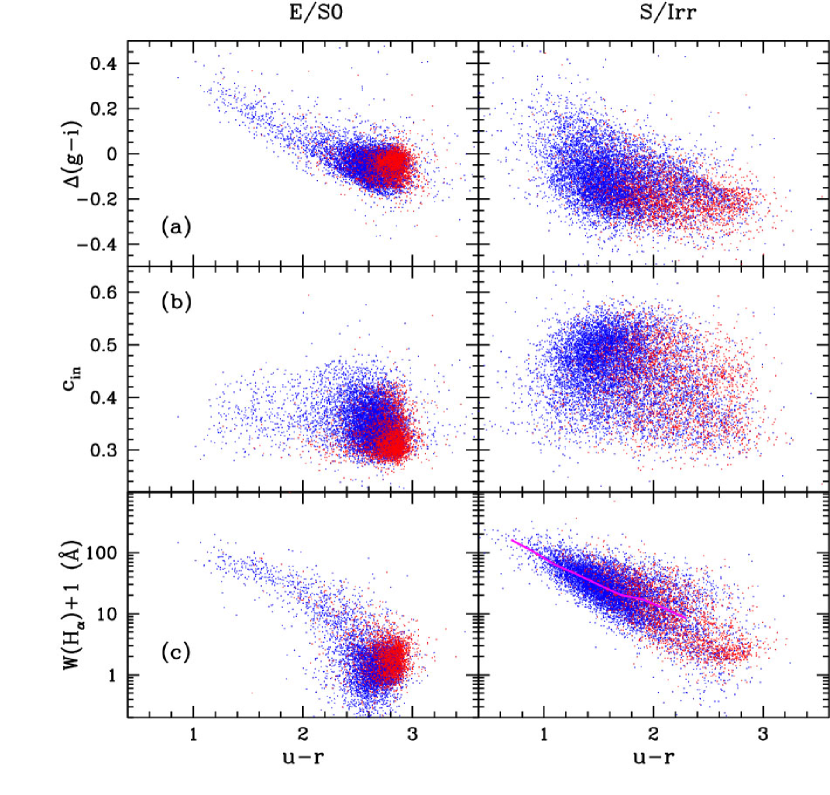
Figure 6.— Relations between the $u-r$ color and ($a$) $g-i$ color gradient, ($b$) (inverse) concentration index, and ($c$) the equivalent width of the $H{\alpha}$ line. The most likely $H{\alpha}$ equivalent width is drawn for the late types (lower right). Blue points are fainter galaxies with $M_{r}\geq-20.0$, and red points are those with $M_{r}<-20.0$.

Figure 6$b$ shows galaxies in the $u-r$ versus the (inverse) concentration index space. The brightest early types have $u-r\approx 2.9$ and $c_{\rm in}\approx 0.3$. There is a weak tendency for the redder ($2.6\leq u-r\leq 3.0$) bright early types to have smaller $c_{\rm in}$ than the bluer ($2.3\leq u-r\leq 2.6$) fainter ones. Late types are loosely concentrated at $u-r\approx 1.5$ and $c_{\rm in}=0.49$. They have a broad overlap with the region occupied by early type galaxies.

Figure 6$c$ shows the relations between $u-r$ color and the equivalent width of $H{\alpha}$ line, $W(H{\alpha})$. Most red early type galaxies have weak emission, $W(H{\alpha})<3$. Because galaxies in the blue trail of early types usually have blue star-forming centers, $W(H{\alpha})$ in the light from their centers has a tight correlation with their color. The right panel of Figure 6c shows that the $H{\alpha}$ emission line strength of the centers of late type galaxies (plotted as $\log[W(H\alpha)]$) is close to being linearly proportional to the overall $u-r$ color. This is particularly true for blue late types. This proportionality is as expected if $H{\alpha}$ emission is proportional to $u$-band luminosity. It is interesting to observe that the sequence formed by the blue early types is far from a straight line and has higher $W(H{\alpha})$ than the sequence of the blue late types.

3.3. Velocity Dispersion of Early Types

Stellar velocity dispersion is a dynamical indicator of the mass of galaxies. Figure 7$a$ shows that there is a good correlation between velocity dispersion and concentration index, and thus between mass and surface brightness profile. Here it should be noted that the D2 sample starts to be incomplete at $\sigma\leq 150$ km s^-1 due to the absolute magnitude cut and the significant dispersion of $\sigma$ at a given absolute magnitude (see Fig. 4$b$).

The relation becomes tighter for high-$\sigma$ early type galaxies and approaches the de Vaucouleurs profile value of $c_{\rm{in}}=0.29$ at the highest end. The size of galaxies is well correlated with velocity dispersion when $\sigma>100$ km s^-1, but the dependence become weaker at lower $\sigma$ (Figure 7b). Note that the number of galaxies with $R_{\rm Pet}\leq 3h^{-1}$kpc is underestimated in the D2 sample. The error in $\sigma$ is typically 11 km s^-1 (see below), which somewhat broadens the size versus $\sigma$ relation. These systematic effects should be taken into account in interpreting Figure 7$b$.

Figure 7$c$ indicates that there are progressively more centrally star-forming early type galaxies as the velocity dispersion decreases, consistent with the relation between $W(H{\alpha})$ and $M_{r}$ (Fig. 4$c$).

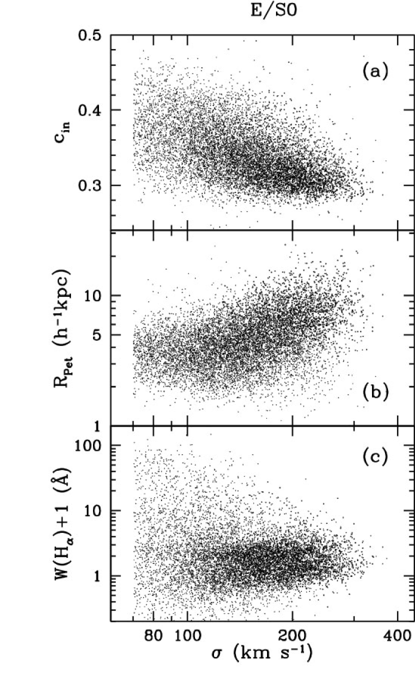
Figure 7.— Relation between the velocity dispersion of early type galaxies in sample D2 and ($a$) (inverse) concentration index, ($b$) the Petrosian radius, and ($c$) the equivalent width of the $H{\alpha}$ line. Larger dots are galaxies with $M_{r}<-20.5$, and smaller dots are those with $M_{r}>-20.5$.

4. Collective Physical Parameters

4.1. Luminosity Function

The upper panel of Figure 8 shows the luminosity function (LF) of galaxies in the D3 sample. Filled circles are the LF measured by using both early and late type galaxies. Open circles are the LF of the E/S0 morphological types, and open squares are that of the S/Irr types. Symbols are calculated by binning galaxies in each magnitude bin. Uncertainty limits are estimated from 16 subsets of each sample. Curves are the best-fit Schechter functions of the following form

$$\phi(L)dL=\phi{{}_{*}}(L/L{{}_{*}})^{\alpha}{\rm exp}(-L/L{{}_{\ast}})dL/L{{}_{\ast}}.$$ (3)

We use the MINUIT package of the CERN program library to determine the parameters in the Schechter function by the maximum likelihood method, which is applied to individual galaxies as described in Sandage et al. (1979). The Schechter function fits the data extremely well except for the highest luminosity bins. To reduce the bias in LF due to the internal absorption, we have included only those late types with axis ratios $b/a>0.6$ in our analyses. To estimate the number density (or $\phi_{\ast}$) of all spiral galaxies, we need to know the fraction of late type galaxies with apparent axis ratios greater than $0.6$. We adopt the fraction $0.505$ calculated from the CM sample (see Fig. 13$b$, below), whose spiral membership is considered to be the least affected by the internal absorption. We use this fraction to scale up the late type galaxy LF estimated by using only those with $b/a>0.6$. The results of the Schechter function fits are summarized in Table 2.

Table 2Total and Type-specific Schechter Function Parameters

Name	Absolute Magnitude	$M_{\ast}-5{\rm log_{10}}{h}$	$\alpha$	$\phi_{\ast}$
				$10^{-2}h^{3}{\rm Mpc}^{-3}$
All Types:
D1	$-18.0>M_{\rm r}$	$-20.31\pm 0.04$	$-0.918\pm 0.027$	$1.64$
D2	$-18.5>M_{\rm r}$	$-20.22\pm 0.03$	$-0.843\pm 0.026$	$1.72$
D3	$-19.0>M_{\rm r}$	$-20.22\pm 0.03$	$-0.807\pm 0.028$	$1.85$
D4	$-19.5>M_{\rm r}$	$-20.28\pm 0.02$	$-0.867\pm 0.030$	$2.01$
D5	$-20.0>M_{\rm r}$	$-20.32\pm 0.02$	$-0.895\pm 0.039$	$1.87$
Early Types:
D1	$-18.0>M_{\rm r}$	$-20.17\pm 0.05$	$-0.494\pm 0.047$	$0.73$
D2	$-18.5>M_{\rm r}$	$-20.16\pm 0.04$	$-0.473\pm 0.044$	$0.71$
D3	$-19.0>M_{\rm r}$	$-20.23\pm 0.04$	$-0.527\pm 0.043$	$0.71$
D4	$-19.5>M_{\rm r}$	$-20.38\pm 0.03$	$-0.719\pm 0.042$	$0.75$
D5	$-20.0>M_{\rm r}$	$-20.49\pm 0.03$	$-0.870\pm 0.052$	$0.66$
Late Types:
D1	$-18.0>M_{\rm r}$	$-20.30\pm 0.05$	$-1.070\pm 0.033$	$0.98$
D2	$-18.5>M_{\rm r}$	$-20.18\pm 0.04$	$-0.965\pm 0.034$	$1.10$
D3	$-19.0>M_{\rm r}$	$-20.12\pm 0.03$	$-0.897\pm 0.037$	$1.23$
D4	$-19.5>M_{\rm r}$	$-20.09\pm 0.03$	$-0.832\pm 0.043$	$1.44$
D5	$-20.0>M_{\rm r}$	$-20.04\pm 0.03$	$-0.666\pm 0.061$	$1.37$

Since our volume-limited samples from the SDSS do not extend to very faint magnitudes, there is a significant correlation between measured $M_{\ast}$ and $\alpha$. We choose the D3 sample to estimate a representative LF of the SDSS galaxies as a compromise; the uncertainty in $M_{*}$ is minimized for D4, while the uncertainty in $\alpha$ is minimized for D2. However, the D3 sample covers the absolute magnitude space brighter than $-19.0$, only about 1.2 mag fainter than $M_{\ast}$, and the correlation between the estimated parameters $M_{\ast}$ and $\alpha$ makes their physical meanings less clear. The LF of the deeper D4 sample, which includes the Sloan Great Wall (Gott et al. 2005), shows the highest density of early type galaxies among all five volume-limited samples, and thus its LF seems less representative. The D5 sample does not extend faint enough to determine the $\alpha$ parameter. The existence of the large scale structure affects both normalization and shape of LF (e.g. Croton et al. 2005). Therefore, the trends in $M_{\ast}$ and $\alpha$ are affected by the fact that nearby universe is a relatively underdense region and the shallower samples are more dominated by the relatively faint galaxies which prefers underdense regions (see Fig. 10 of Paper II for further details). When all spiral galaxies are used (i.e. no internal absorption effect correction), the LF of all galaxies in the D3 sample is well fitted by $M_{\ast}=-20.24\pm 0.03$ and $\alpha=-0.90\pm 0.03$. For comparison, Blanton et al. (2003a) report $M_{\ast}=-20.44\pm 0.01$, and $\alpha=-1.05\pm 0.01$ for an apparent magnitude-limited sample called SDSS LSS Sample 10 (similar to SDSS DR1). If we adopt the faint end slope $\alpha$ from the shallow sample D1 and $M_{\ast}$ from the deepest sample D5, our estimates are $\alpha=-0.99\pm 0.03$ and $M_{\ast}=-20.38\pm 0.03$, which are very close to Blanton et al.’s.

When the internal absorption effect in the sample is reduced, the LF of spirals changes, particularly in the $\alpha$ parameter. The LF of early types in sample D3 has $M{{}_{\ast}}=-20.23\pm 0.04$ and $\alpha=-0.53\pm 0.04$ while that of late types has a fainter characteristic magnitude of $M{{}_{*}}=-20.12\pm 0.03$ and a steeper faint-end slope of $\alpha=-0.90\pm 0.04$. If all spiral galaxies are used, the LF of late types has $M{{}_{*}}=-20.09\pm 0.04$ and $\alpha=-1.01\pm 0.04$. This demonstrates that the faint-end slope $\alpha$ of late types would have been misleadingly measured steeper if the inclined late type galaxies had not been excluded. The blue galaxies classified as early types by our morphological classifier make an increasing contribution to the LF at faint magnitudes. We suspect that some of these objects are actually bulge-dominated spirals whose disks are lost to the background sky. However, the absolute contribution of blue early type galaxies to the LF is still small at the magnitudes studied, as seen in Figure 3$a$, and the type-specific LFs at magnitudes brighter than $M_{r}=-18$ seems well determined by our samples. Baldry et al. (2004) used $u-r$ color-selected early (red) and late (blue) type galaxy samples to measure their luminosity functions. The estimated $M_{\ast}$ parameter differed by 0.21 mag and the $\alpha$-parameter was measured to be $-0.83$ (early) and $-1.18$ (late). The difference in $M_{\ast}$ between early and late types is quite consistent with our result, but they obtained steeper $\alpha$’s.

The bottom panel of Figure 8 shows the fraction of E/S0 galaxies in all five volume-limited samples as a function of $r$-band absolute magnitude. Again, only late types with $b/a>0.6$ are used, and their number fraction of 0.505 is used to infer the total number of spiral galaxies. There is a surprisingly consistent monotonic relation between luminosity and early type galaxy fraction. The critical magnitude at which the early type fraction exceeds 50% is $M_{r}=-21.29\pm 0.04$. Even though the shape of LF itself shows significant fluctuations due to large scale structures when measured in different regions of the universe, the morphological fraction as a function of luminosity is relatively less sensitive to large scale structures and thus seems to be more universal. However, it is well-known that the early type fraction is a monotonically increasing function of local density (Dressler 1980; Tanaka et al. 2005; Goto et al. 2003a; Paper II). Weinmann et al. (2006) also measured the morphology fraction as a function of $M_{r}$ and found basically the same dependence, even though the sample they used is smaller.

Figure 8.— Top: Luminosity function (LF) of galaxies in the D3 sample. Filled circles are for all galaxies, open circles for the E/S0 morphological types, and open squares for the S/Irr types. Symbols are the LF calculated by binning galaxies in each magnitude bin. Curves are the best-fit Schechter functions. Bottom: The elliptical galaxy fraction in magnitude bins measured from the five volume-limited samples (D1 - D5).

4.2. Velocity Dispersion Function

The velocity dispersion function (VDF) of early type galaxies can be used to derive gravitational lens statistics and to estimate cosmological parameters. To estimate the velocity dispersion function we need to have a sample of galaxy velocity dispersion data that is complete over a wide range. Figure 4$b$ indicates that sample D2, for example, starts to be incomplete at $\sigma\leq 150$ km s^-1 due to the absolute magnitude cut and the significant dispersion of $\sigma$ at a given absolute magnitude. To lower the completeness limit down to $\sigma\approx 70$ km s^-1 we have used a series of our volume-limited samples an additional very faint volume-limited sample with $-16.8\geq M_{r}>-17.5$, which is added because even the CM sample is not faint enough to give the $\sigma$-distribution complete down to $\sigma=70$ km s^-1. The differences in volumes of these volume-limited samples are taken into account when we estimate the velocity dispersion function from a combination of seven samples.

The circles in Figure 9 show the VDF of early type galaxies measured in this way.

Figure 9.— Velocity dispersion functions (VDFs; circles) measured from our samples with galaxies brighter than $M_{r}=-16.8$. The solid curve is our estimate of the true VDF best fit by a modified Schechter function. The long-dashed curve is the best fit to the raw measurement. The dotted curve is the fit given by Sheth et al. (2003).

Figure 10.— Histogram showing the distributions of the standard deviations of $\sigma$ of the galaxies measured by two different SDSS pipelines IDLSPEC2D (thin and thick solid lines) and SPECTRO1D (dotted line). The thick solid and dotted lines are obtained from the repeat measurements (plate 406 and 412) and the thin solid line is from the formal error given by the IDLSPEC2D.

The curve is the fit by a modified Schechter function of the form

$$\phi(\sigma)d\sigma=\phi{{}_{\ast}}(\sigma/\sigma{{}_{\ast}})^{\alpha}{\rm exp}[-(\sigma/\sigma{{}_{\ast}})^{\beta}]{\beta\over\Sigma(\alpha/\beta)}{d\sigma\over\sigma},$$ (4)

where $\sigma{{}_{\ast}}$ is the characteristic velocity dispersion, $\alpha$ is the low-velocity power-low index, and $\beta$ is the high-velocity exponential cutoff index (Mitchell et al. 2005). The VDF parameters obtained by the MINUIT package are

$$(\phi_{\ast},\sigma_{\ast},\alpha,\beta) = (8.0\times 10^{-3}h^{3}{\rm Mpc}^{-3},~{}~{}161\pm 5{\rm kms^{-1}},$$

$$2.32\pm 0.10,~{}~{}2.67\pm 0.07).$$

When we made the fit with the above parameters, we assumed that the measurement error in $\sigma$ was approximated by $0.084\sigma$ km s^-1 (see below). The dashed curve in Figure 9 is the modified Schechter function best fit to the raw data points (open circles) which are broadened at high $\sigma$’s due to the measurement error. The solid curve is the deconvolved VDF whose parameters are given above.

It should be noted that there exists very strong correlations among the fitting parameters, and the results of the fitting depend sensitively on the range of the velocity dispersion used. Our estimate of the VDF of early type galaxies is quite different from that of Sheth et al. (2003) and Mitchell et al. (2005). The dotted curve in Figure 9 is the VDF best fit given by Sheth et al. (2003). Mitchell et al. (2005) presented the same function with the normalization $\phi_{\ast}$ lowered by 30%. The difference at small $\sigma$ seems due to the fact that some of morphologically early type galaxies are discarded based on spectrum in Sheth et al. (cf. Fig. 12 of Mitchell et al. 2005). It is not clear what makes the difference at large $\sigma$, but it could be due to the measurement error larger than that adopted here.

In order to check whether or not our VDF is seriously affected by the measurement error in $\sigma$ we have made the following test. We first adopt Sheth et al. (2003)’s VDF as the true one. We then look for galaxies having 4 or 5 repeat measurements of $\sigma$ in southern stripe 82 (plates 406 and 412) to estimate the error. The thick histogram in Figure 10 shows the distribution of the standard deviations of $\sigma$ of the galaxies with repeat measurements. The median size of error is 11 km s^-1. One can note that the error estimated from the repeat measurements by the IDLSPEC2D is larger than the formal error (thin histogram) given by the IDLSPEC2D, but is comparable with that (dotted histogram) obtained from the repeat measurements by the official spectroscopic pipeline, SPECTRO1D (written by M. SubbaRao, M. Bernardi and J. Frieman). If the measurement error were larger than 20 km s^-1, the dispersion of the relation between $M_{r}$ and $\sigma$ shown in Figure 4$b$ would be much larger. We then calculate the VDF affected by the error in $\sigma$.

Figure 11.— Velocity dispersion functions (VDFs) demonstrating the effect of the measurement errors in $\sigma$ on the VDF. The dotted curve is Sheth et al.(2003)’s VDF, and the short-dashed curve is the VDF deformed due to the Gaussian-distributed measurement error of $0.084\sigma$ km s^-1. The long-dashed curve is the best fit to the VDF measured in this work.

The dotted curve in Figure 11 is Sheth et al.’s function, and the short-dashed curve is the VDF deformed due to the Gaussian-distributed measurement error of $0.084\sigma$ km s^-1, which reflects the fact that the error in $\sigma$ estimated from the repeat measurements increases as $\sigma$ increases. It demonstrates that our VDF cannot be realized from Sheth et al.’s function by the convolution effects of the measurement error

4.3. Axis Ratio Distribution

The scatter plot of galaxies in Figure 5 indicates that the mean axis ratio of bright late type galaxies tend to be high. This is due to the internal absorption making inclined galaxies appear fainter. The bottom panel of Figure 12 shows the late type galaxies of sample D3 in the $M_{r}$ versus $u-r$ color space as in the right panel of Figure 3$a$. Galaxies with $b/a>0.8$ are shown as blue dots, and those with $b/a<0.4$ are shown as red dots. Their most likely color curves are also drawn. We find that the group of highly inclined galaxies is significantly shifted with respect to the almost face-on ones toward fainter magnitudes and redder colors. We also find that the shapes of the two distributions are different, which can be explained if the galaxies with intermediate magnitude ($M_{r}\sim-20.5$) and color ($u-r\sim 1.6$) suffer from more dimming and reddening due to internal extinction. The color of very red or very blue galaxies seems to be less affected by the internal extinction. A detailed study of internal extinction is needed for the SDSS galaxies. The early types are not much affected. If one does not take into account this inclination effect on magnitude, the measured LF of late type galaxies and the morphology fraction will be seriously in error. In analyses where these systematics are important, we have used late types with $b/a>0.6$. Figure 5 demonstrates that the inclination effects on magnitude is small for this set of late type galaxies.

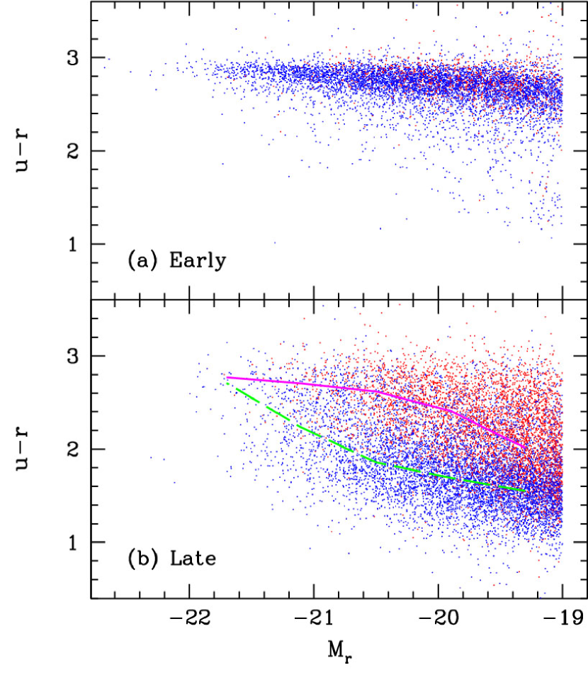
Figure 12.— Distributions of ($a$) early and ($b$) late type galaxies in the color magnitude diagram. Galaxies with $b/a>0.8$ are shown as blue dots, and those with $b/a<0.4$ are shown as red dots. For late types the most likely color-magnitude relations are drawn for the different axis ratio sets.

Figure 13.— Distributions of the apparent isophotal axis ratio of ($a$) early and ($b$) late type galaxies.

Because of the inclination effects on magnitude, our volume-limited samples are not complete for late type galaxies near the absolute magnitude cuts. The lower panel of Figure 13 shows distributions of isophotal axis ratio of late type galaxies in samples CM (solid line with filled circles), D2 (short-dashed line with open circles), and D4 (long-dashed line with open squares). There appears to be no late type galaxy with nearly zero axis ratio because of the intrinsic thickness of disks of late type galaxies. The axis ratio of 0.2 due to the intrinsic thickness is consistent with previous works (Sheth et al. 2003). Almost face-on galaxies are also lacking, because disks of late type galaxies do not appear exactly round even when they are face-on (Kuehn & Ryden 2005). The distributions are significantly different from one another because of the internal absorption effects, lacking highly inclined galaxies in the samples with bright cuts. We assume that the magnitude limit of CM sample ($M_{r,{\rm cut}}=-17.5$) is faint enough that its $b/a$ distribution is close to the intrinsic distribution. The fraction of galaxies with $b/a>0.6$ in the CM sample is 0.505. The upper panel of Figure 13 shows the distribution of projected axis ratio of early type galaxies. Distributions obtained from three samples with different magnitude cuts match one another very well. This reflects the fact that internal absorption in early type galaxies is negligible.

Alam & Ryden (2002) measured the axis ratio distributions for red and blue populations in the SDSS EDR sample. The distribution functions for red or blue galaxies well-fitted by a de Vaucouleurs profile match well with our result for early types. Sheth et al. (2003) also measured the distribution of axis ratio of early and late type galaxies in the SDSS. Their axis ratio distribution of early types agrees well with ours except at the $b/a=1$ bin.

5. Summary

We have elaborately investigated the relations among various internal (e.g. color, luminosity, morphology, star formation rate, velocity dispersion, size, radial color gradient, and axis ratio) and collective properties (e.g. luminosity function, velocity dispersion distribution function, and axis ratio distribution function). We will study other collective properties such as the correlation function, power spectrum, topology, and peculiar velocity field, in separate works.

There are a number of important improvements we made in our measurement:

1. To extend the absolute magnitude range, we have added the redshifts of the bright galaxies with $r<14.5$ to the SDSS-NYU-VAGC. Six volume-limited samples with faint limits from $M_{r}=-17.5$ to $-20.0$, are used for more efficient use of the flux-limited SDSS sample.

2. We have divided the samples into subsamples of early (E/S0) and late (S/Irr) morphology types by using our accurate morphology classifier, working in the three-dimensional parameter space of $u-r$ color, $g-i$ color gradient, and concentration index. The morphology classifier is able to separate the blue early types from the blue late types, and also to distinguish the spirals from the red E/S0 types because it does not depend only on color.

3. The late type galaxies with isophotal axis ratio of less than 0.6 have been excluded because they suffer severely from dimming and reddening due to internal extinction and then may cause biases in luminosity, luminosity function, color, color gradient, and so on. This correction makes the blue sequence of the late type galaxies bluer and brighter compared to that obtained from all late type galaxies. The blue sequence also become better-defined with smaller width.

We have found that absolute magnitude and morphology are the most important parameters in characterizing physical properties of galaxies. In other words, other parameters show relatively small scatter once absolute magnitude and morphology are fixed for early type galaxies, in particular. One very interesting fact we have noticed in our work is that many physical parameters of galaxies manifest different behaviors across the absolute magnitude of about $M_{\ast}\pm 1$. For example, the red sequence of early types changes the slope at $M_{\rm r}\approx-19.6$ in the color-magnitude space. Also, at a magnitude fainter than $M_{\rm r}\sim-20$, the number of blue star-forming early types increases significantly, and the surface brightness profile as parameterized by $c_{\rm in}$ becomes less centrally concentrated. The passive spirals with vanishing $H_{\alpha}$ emission seem to have magnitudes brighter than $M_{\rm r}\sim-19.5$.

At fixed morphology and luminosity, we find that bright ($M_{r}<-20$) early type galaxies show very small dispersions in color, color gradient, concentration, size, and velocity dispersion. These dispersions increase at fainter magnitudes, where the fraction of blue star-forming early types increases. Concentration indices of early types are well-correlated with velocity dispersion, but are insensitive to luminosity and color for bright galaxies, in particular. The slope of the Faber-Jackson relation ($L\propto{\sigma}^{\gamma}$) continuously changes from $\gamma=4.6\pm 0.4$ to $2.7\pm 0.2$ when luminosity changes from $M_{r}=-22$ to $-20$. The size of early types is well-correlated with stellar velocity dispersion, $\sigma$, when $\sigma>100$ km s^-1. Late type galaxies show wider dispersions in all physical parameters compared to early types at the same luminosity. We find that passive spiral galaxies are well-separated from star-forming late type galaxies at $H{\alpha}$ equivalent width of about 4.

We note that the estimated LF shows significant fluctuations due to large scale structures when measured in different regions of the universe. On the other hand, the morphological fraction as a function of luminosity is relatively less sensitive to large scale structures and thus seems to be more universal. In Paper II, it is shown that the morphology fraction is a monotonic function of local density at a fixed luminosity. Since luminosity in turn depends on local density, this result indicates that the probability for a galaxy to be born as a particular morphological type is basically determined when its luminosity or mass is given. To this extent, morphology is determined by galaxy mass. The question here is what determines the morphology of a galaxy having a particular mass while keeping the type fraction corresponding to its mass scale. Further investigations are required to answer this question.

References

- (1) Abazajian, K., et al. 2004, AJ, 128, 502
- (2) Adelman-McCarthy, J. K., et al. 2006, ApJS, 162, 38
- (3) Alam, S. M. K., & Ryden, B. S. 2002, ApJ, 570, 610
- (4) Baldry, I. K. et al., 2004, ApJ, 600 681
- (5) Balogh, M. L., et al. 2004a, ApJ, 615, L101
- (6) Balogh, M. L., et al. 2004b, MNRAS, 348, 1355
- (7) Bernardi, M., Sheth, R. K., Nichol, R. C., Schneider, D. P., & Brinkmann, J. 2005 AJ, 129, 61
- (8) Bernardi, M., et al. 2003a, AJ, 125, 1866
- (9) Bernardi, M., et al. 2003b, AJ, 125, 1817
- (10) Blanton, M. R., et al. 2005, AJ, 129, 2562
- (11) Blanton, M. R., et al. 2003a, ApJ, 594, 186
- (12) Blanton, M. R., Lin, H., Lupton, R. H., Maley, F. M., Young, N., Zehavi, I., & Loveday, J. 2003b, AJ, 125, 2276
- (13) Blanton, M. R., et al. 2003c, AJ, 125, 2348
- (14) Couch W. J., Barger A. J., Smail I., Ellis R. S., Sharples R. M., 1998, ApJ, 497, 188
- (15) Colless, M., et al. 2001, MNRAS, 328, 1039
- (16) Croton, D. J., et al. 2005, MNRAS, 356, 1155
- (17) Desroches, L.-B., Quataert, E., Ma, C.-P., & West, A. A. 2006, astro-ph/0608474
- (18) Dressler, A., 1980, ApJ, 236, 351
- (19) Eisenstein, D. J., et al. 2001, AJ, 122, 2267
- (20) Falco, E. E., et al. 1999, PASP, 111, 438
- (21) Fukugita, M., Ichikawa, T., Gunn, J. E., Doi, M., Shimasaku, K., & Schneider, D. P. 1996, AJ, 111, 1748
- (22) Fukugita, M., Nakamura, O. Turner, E. L., Helmboldt, J., Nichol, R. C. 2004 ApJ, 601, 127L
- (23) Gómez, P., et al. 2003, ApJ, 584, 210
- (24) Gott, J. R., Juric, M., Schlegel, D., Hoyle, F., Vogeley, M. S., Tegmark, M., Bahcall, N., & Brinkmann, J. 2005, ApJ, 624, 463
- (25) Goto 2005 MNRAS357, 937
- (26) Goto, T., et al. 2003a,MNRAS, 346, 601
- (27) Goto, T., et al. 2003b, PASJ, 55, 757
- (28) Goto, T., et al. 2003c, PASJ, 55, 771
- (29) Gunn, J. E., et al. 2006, AJ, 131, 2332
- (30) Gunn, J. E., et al. 1998, AJ, 116, 3040
- (31) Hogg, D. W., Finkbeiner, D. P., Schlegel, D. J., & Gunn, J. E. 2001, AJ, 122, 2129
- (32) Hogg, D. W., et al., 2004, ApJ, 601, L29
- (33) Ivezić, Z., et al. 2004, AN, 325, 583
- (34) Jørgensen, I., Franx, M., & Kjærgaard, 1995, MNRAS, 276, 1341
- (35) Kuehn, F. & Ryden, B. S. 2005 ApJ, 634, 1032
- (36) Lewis, I., et al. 2002, MNRAS, 334, 673
- (37) Lupton, R. H., Gunn, J. E., Ivezić, Z., Knapp, G. R., Kent, S., & Yasuda, N. 2001, in ASP Conf. Ser. 238, Astronomical Data Analysis Software and Systems X, ed. F. R. Harnden, Jr., F. A. Primini, & H. E. Payne (San Francisco: ASP), 269
- (38) Madgwick D. S., et al., 2002, MNRAS, 333, 133
- (39) Mitchell, J. L., Keeton, C.R., Frieman, J.A., & Sheth, R.K, 2005, ApJ, 622, 81
- (40) Nakamura, O., et al. 2003, ApJ, 125, 1682
- (41) Park, C., et al., 2006, ApJ, submitted (Paper II)
- (42) Park, C., & Choi, Y.-Y., 2005, ApJ, 635, L29
- (43) Pier, J. R., Munn, J. A., Hindsley, R. B., Hennessy, G. S., Kent, S. M., Lupton, R. H., & Ivezic, R. 2003, AJ, 125, 1559
- (44) Poggianti, B. M., Smail, I., Dressler, A., Couch, W. J., Barger, A. J., Burtcher, H., Ellis, R. S., & Oemler, A., Jr. 1999, ApJ, 518, 576
- (45) Quintero, A. D., et al., 2004, ApJ, 602, 190
- (46) Richards, G. T., et al., 2002, AJ, 123, 2945
- (47) Sandage, A., Tammann, G. A., & Yahil, A., 1979, ApJ, 232, 352
- (48) Saunders, W. et al. 2000, MNRAS, 317, 55
- (49) Schlegel, D. J., Finkbeiner, D. P., & Davis, M. 1998, ApJ, 500, 525
- (50) Shen, S., et al. 2003, MNRAS, 343, 978
- (51) Sheth, R. K., et al. 2003, ApJ, 594, 225
- (52) Smith, J. A., et al. 2002, AJ, 123, 2121
- (53) Stoughton, C., et al. 2002, AJ, 123, 485
- (54) Strauss, M. A., et al. 2002, AJ, 124, 1810
- (55) Tanaka, M., et al. 2004, AJ, 128, 2677
- (56) Tegmark, M., et al. 2004, ApJ, 606,702
- (57) Tucker, D., et al. 2006, AN, in press
- (58) Weinmann, S. M., van der Bosch, F. C., Yang, X., & Mo, H. J. 2006, MNRAS, 366, 2
- (59) Yamauchi, C., & Goto, T. 2005, MNRAS, 359, 1557
- (60) Yamauchi, C., & Goto, T. 2004, MNRAS, 352, 815
- (61) York, D., et al. 2000, AJ, 120, 1579