A Broadband Study of Galactic Dust Emission

We have combined infrared data with H_I, H₂ and H_II surveys in order to spatially decompose the observed dust emission into components associated with different phases of the gas. An inversion technique is applied. For the decomposition, we use the IRAS 60 and 100 $\mu$m bands, the DIRBE 140 and 240 $\mu$m bands, as well as Archeops 850 and 2096 $\mu$m wavelengths. In addition, we apply the decomposition to all five WMAP bands. We obtain longitude and latitude profiles for each wavelength and for each gas component in carefully selected Galactic radius bins. We also derive emissivity coefficients for dust in atomic, molecular and ionized gas in each of the bins. The H_I emissivity appears to decrease with increasing Galactic radius indicating that dust associated with atomic gas is heated by the ambient interstellar radiation field (ISRF). By contrast, we find evidence that dust mixed with molecular clouds is significantly heated by O/B stars still embedded in their progenitor clouds. By assuming a modified black-body with emissivity law $\lambda^{-1.5}$, we also derive the radial distribution of temperature for each phase of the gas. All of the WMAP bands except W appear to be dominated by emission from something other than normal dust, most likely a mixture of thermal bremstrahlung from diffuse ionized gas, synchrotron emission and spinning dust. Furthermore, we find indications of an emissivity excess at long wavelengths ($\lambda\geq$ 850 $\mu$m) in the outer Galaxy (R $>$ 8.9 kpc). This suggests either the existence of a very cold dust component in the outer Galaxy or a temperature dependence of the spectral emissivity index. Finally, it is shown that $\sim$ 80$\%$ of the total FIR luminosity is produced by dust associated with atomic hydrogen, in agreement with earlier findings by Sodroski et al. (1997).
The work presented here has been carried out as part of the development of analysis tools for the planned European Space Agency (ESA) Planck mission.

1 Introduction

The release (Neugebauer et al. 1984) of the Infrared Astronomical Satellite (IRAS) maps (at 12, 25, 60 and 100 $\mu$m) provided a new perspective on the Galactic interstellar medium (ISM) by revealing diffuse infrared emission over almost the entire sky. This finding was confirmed (Hauser 1993) by the Diffuse Infrared Background Explorer (DIRBE) experiment (1.25 to 240 $\mu$m) on board the COBE satellite. Even in the lowest 12-$\mu$m IRAS band, stellar radiation contributes only a small fraction ($\sim$ 8$\%$) of the emission (Boulanger $\&$ Perault 1988), the rest is from ISM. This fact is also corroborated by the tight correlations found by Boulanger et al. 1996 at high Galactic latitudes, i.e. $|b|>$ 20^∘, between the 100 $\mu$m emission and the 21-cm emission, the latter being a faithful tracer of HI. By using a fixed spectral emissivity index $\beta$=2, these authors derive a temperature for dust associated with HI of 17 K. A similar correlation has been found for high-latitude molecular clouds, their CO emission being tightly correlated with the 100 $\mu$m intensity distribution (e.g. Boulanger et al. 1996). Likewise, Lagache et al. (2000) detect dust emission from the Warm Ionized Medium for $b<$ -30^∘, $b>$ 25^∘, with physical properties (temperature and emissivity) similar to dust associated with atomic hydrogen. Remarkably, most of this dust emission is not contributed by discrete H_II regions but by the diffuse gas.

As one can notice, all the results mentioned above have been obtained at high latitudes. In fact, the Galactic plane in in general much more complicated to investigate. This is because at high latitudes each line of sight traces a relatively short path through the Galaxy and this makes it possible to probe each distinct phase of the gas separately. On the contrary, in the Galactic plane the lines of sight are much longer and the phases of the gas heavily blended. A solution to this problem has been provided by the maximum-likelyhood method worked out by Bloemen et al. (1986). This method allows one to spatially decompose the total infrared emission into components associated with atomic, molecular and ionized gas in different bins of Galactic radiu. A similar technique is used in this paper and will be described in Section 2.

Another important observational fact derived from IRAS data is that most of the IR luminosity falls at $\lambda$ $>$ 60 $\mu$m. In particular, $\sim$ 50$\%$ of the IRAS luminosity is observed at $\lambda>$ 100 $\mu$m and only one sixth in each of the other bands. According to a variety of dust grain models (e.g. Mathis et al. 1977, Draine $\&$ Lee 1984, Draine $\&$ Anderson 1985; Weiland et al. 1986; Desert et al. 1990; Li $\&$ Greenberg 1997; Dwek et al. 1997; Draine $\&$ Li 2001; Zubko, Dwek $\&$ Arendt 2004) the 12 $\mu$m emission is dominated by PAHs (Polycyclic Aromatic Hydrocarbons) which are characterized by a size of order of a few nanometers, while at 100 $\mu$m the emission is mainly due to large grains, typically in the size range 10-20 nm to 0.1 $\mu$m. Intermediate wavelengths (25-60 $\mu$m) are instead the domain of VSGs (Very Small Grains), in the nanometer range. Therefore, IRAS data indicate that most of the emission is undisputedly due to large grains. IRAS has also revealed a wide range of infrared dust colors from 12 to 100 $\mu$m (Boulanger et al. 1990). This can be explained through variations in the dust size distribution. However, the same phenomenon has also been observed at submillimeter wavelengths (200, 260, 360 and 580 $\mu$m) by the PRONAOS balloon-borne experiment (Bernard et al. 1999, Stepnik et al. 2001) and it has been interpreted as due to changes in the physical properties of the large grains themselves, i.e. grain composition and temperature as well as optical properties.

The present work is motivated by several factors. In recent years there has been an unprecedented number of new centimeter and sub-millimeter experiments producing a large amount of data. Among these are the Archeops (Benoit et al. 2002) ballon-borne experiment and the WMAP (Wilkinson Microwave Anisotropy Probe) satellite (Bennett et al. 2003a). Such experiments have provided maps of the sky in the frequency range 23 to 545 GHz (i.e. $\sim$ 10 mm down to 550 $\mu$m) at an angular resolution, depending on frequency, from $\sim$ 50 down to $\sim$ 10 arcmin. Since most of the infrared emission is emitted at $\lambda>$ 60-100 $\mu$m, the combination of these maps with existing IRAS and DIRBE maps now allows one to trace completely the dust spectrum in the frequency range where most of the emission is concentrated. At the same time, new all-sky data have also been released for the H_I emission (Section 3.1) and great progress has been made in observing and modeling the ionized gas (Section 3.3). However, the most significant step forward has probably been in our understanding of the physics of dust grains. With respect to the color variations mentioned above, PRONAOS has also shed light on the dust emissivity index $\beta$: a significant inverse correlation between $\beta$ and dust temperature has been observed in the direction of star forming regions (Dupac et al. 2001). At the same time, analysis of the FIRAS data shows that, in the Galactic plane region, $\beta$ is best-fitted by a value of 1 (Reach et al. 1995) rather than 2 as usually assumed. These are very important findings that alone provide sufficient motivation for revisiting the problem of decomposing the Galactic infrared emission. Further motivation is provided by the impending Planck mission (http//www.rssd.esa.int/ planck) which will obtain high-sensitivity, high-resolution ($\sim$ 5 to 30 arcmin) all-sky maps in the wavelength range $\sim$ 400 $\mu$m - 10 mm. Due to its unique instrumental performance, Planck will provide unprecedented insights on the radio/infrared emission of the diffuse ISM of our Galaxy. The present work was carried out as part of a larger effort to develop tools for the full exploitation of the Planck data.

The paper is organized as follows. Section 2 describes the inversion technique, including a brief review of previous works. In Section 3 we provide details regarding the datasets used, with particular attention given to the ionized gas. Section 4 presents our main results while Section 5 provides conclusions and perspectives.

2 The inversion technique

Along the Galactic plane, the detected infrared emission is a blend of radiation arising from dust that is spread over a wide range of distances and Galactic radii, and subject to a wide range of physical conditions. The purpose of the present study is to decompose this integrated infrared emission into radial bins associated with each phase of the interstellar gas and determine the physical properties of each phase in each bin. This goal can be achieved by means of a so-called inversion method that employs kinematic distances to assign gas to radial bins and require that the gas distributions in the adopted bins have distinctly different spatial distributions. The inversion technique has been first applied to astrophysical data by Bloemen et al. (1986) to determine the Galactocentric distribution of gamma-ray emissivity. Subsequently, Bloemen et al. (1990), Giard et al. (1994) and Sodroski et al. (1997) have used the same method to reconstruct the radial distribution of infrared emission. In the following, we will adopt the mathematical formalism introduced by these authors to describe in detail this technique.

Let $I_{\lambda}$ be the observed emission at wavelength $\lambda$ for a pixel $j$ of a map. Then the modeled emission $Im_{\lambda}$ for this pixel can be written as:

$$Im_{\lambda} = \sum_{i=1}^{n}\left(\epsilon_{H_{\sc{I}}}(R_{i},\lambda){N^{i}_{H_{\sc{I}}}}+\right.$$

$${}\left.\epsilon_{H_{\sc{2}}}(R_{i},\lambda){N^{i}_{H_{\sc{2}}}}+\epsilon_{H_{\sc{II}}}(R_{i},\lambda){N^{i}_{H_{\sc{II}}}}\right)$$

In the expression above: $i$ denotes the intervals (or rings) of galactocentric radii $R_{i}$ over which the decomposition is performed; $\epsilon_{H_{\sc{I}}}(R_{i},\lambda)$, $\epsilon_{H_{\sc{2}}}(R_{i},\lambda)$, $\epsilon_{H_{\sc{II}}}(R_{i},\lambda)$ are the dust emissivities associated with the different phases of the gas in each ring; ${N^{i}_{H_{\sc{I}}}}$ represents the H atom column density for neutral atomic hydrogen (H_I) in the interval $R_{i}$; similarly, ${N^{i}_{H_{\sc{2}}}}$ is the H atom column density for molecular hydrogen (H₂) and ${N^{i}_{H_{\sc{II}}}}$ is the H atom column density for ionized hydrogen (H_II) in the considered ring.

Note that eq. (1) does not require resolution of the kinematic distance ambiguity for material within the solar circle, since we assume that the dust properties vary only with Galactic radius. In addition, following Giard et al. (1994) and Sodroski et al. (1997) we do not assume a constant ratio between $\epsilon_{H_{\sc{I}}}(R_{i},\lambda)$ and $\epsilon_{H_{\sc{2}}}(R_{i},\lambda)$, rather these parameters are allowed to vary in each galactocentric ring. The dust emissivities can be determined by means of a least-square fit analysis, i.e., by minimization of the quantity:

$$\chi^{2}=\sum_{j=pixels}\frac{({Im(j)}_{\lambda}-{I(j)}_{\lambda})^{2}}{{\sigma_{j}}^{2}}$$ (2)

over the map. In the expression above, $\sigma_{j}$ ($\sigma_{j}$ = $\sigma_{j}$($\lambda$)) represents the noise per pixel for the I_λ map (see Section 4.1 for details).

Column densities are computed, for every ring and for each phase of the gas, by applying a circular rotation model for the Galaxy. The rotational velocity $\theta(R)$ of a gas element in differential motion with respect to the Galactic center is given by:

$$\theta(R)=\frac{R}{R_{0}}\left(\theta_{0}+\frac{V_{LSR}}{\sin{l}\hskip 2.84544pt\cos{b}}\right)\hskip 56.9055pt[km/s]$$ (3)

with $R$ the galactocentric distance of the considered gas element, $R_{0}$ the galactocentric distance of the Sun (we take $R_{0}$ = 8.5 kpc), $\theta_{0}$ the rotational velocity of the Sun (we assume $\theta_{0}$ $\simeq$ 220 km/s), $V_{LSR}$ the linear velocity along the line of sight in the Local Standard of Rest and $l$ and $b$ the Galactic coordinates for a given direction. We adopt the rotation curve $\theta(R)$ by Fich, Blitz $\&$ Stark (1989) for which the galactocentric distance can be expressed as:

$$R=\left(\frac{221.641\times R_{0}}{\theta_{0}+0.44286\times R_{0}+\frac{V_{LSR}}{\sin{l}\hskip 2.84544pt\cos{b}}}\right)\hskip 34.14322pt[kpc]$$ (4)

Therefore, given a specified ring $R_{i}$, the corresponding range in linear velocities is:

$$V^{i}_{LSR} = 221.641\times\frac{R_{0}}{R_{i}}+\hskip 68.28644pt[km/s]$$

$${}-\sin{l}\cos{l}(\theta_{0}+0.44286\times R_{0})$$

For each given ring, ${N^{i}_{H_{\sc{I}}}}$, ${N^{i}_{H_{\sc{2}}}}$ and ${N^{i}_{H_{\sc{II}}}}$ are then computed by integration over the velocity channels selected as above. Further details, specific to each gas phase, will be given in the following section. We note that the use of a different rotation model would not significantly affect the results of the analysis. For the ring decomposition, we have chosen the following intervals:

$$R_{i} = \left[\hskip 2.84544pt[0.1,4],[4,5.6],[5.6,7.2],[7.2,8.9],\right.\hskip 14.22636pt[kpc]$$

$${}\left.[8.9,14],[14,17]\hskip 2.84544pt\right]$$

The above decomposition has been obtained through a process of optimization of the number and type of Galactocentric intervals aimed at reducing the cross-correlation between neighboring rings and therefore leading to a well-defined linear inversion problem. This goal has been achieved by starting with a fine decomposition (roughly 200 bins in Galactic radius) and then gradually combining correlated rings, guided by the eigenvalues of the cross-correlation matrix for different components.

All the maps used for the inversion have been projected into HEALPix format (Gorski et al. 1999) and degraded to 1^∘ resolution. The final maps (input IR maps as well as H_I, H₂ and H_II galactocentric-annuli maps) are at the HEALPix resolution (i.e. nside) 256 which roughly corresponds to a pixel linear size of 13.7^′.

3 The data base

3.1 Dust

To trace dust emission we use a large data base ranging from sub-millimeter to centimeter wavelengths. At short wavelengths, i.e. 60 and 100 $\mu$m, we use the last generation of IRAS plates, the so-called IRIS (Improved Reprocessing of the IRAS Survey) maps (Miville-Deschenes $\&$ Lagache, 2005). These maps have been obtained by reprocessing the original ISSA plates in a manner that allowed the correction for calibration, zero level and striping problems. The IRIS maps (which are at an angular resolution of 4-arcmin at 60 $\mu$m and 4.3-arcmin at 100 $\mu$m) also have a better zodiacal light subtraction. At 140 and 240 $\mu$m, we use the DIRBE Zodi-Subtracted Mission Average Maps. DIRBE is a photometer on-board the COBE satellite with a resolution of 40-arcmin. To probe the sub-millimeter wavelengths, we make use of Archeops data. Archeops is a ballon-borne experiment (Benoit et al. 2002) which has detected Cosmic Microwave Background (CMB) anisotropies at the average angular resolution of 8-arcmin in 4 frequency bands, 143, 217, 353 and 545 GHz. It is the only experiment of this kind which has provided information on the Galactic plane emission at millimeter wavelengths over a large fraction of the sky. Three flights have been performed: a first one (T99) in July 1999 from Trapani (Italy) followed by a second one (KS1) in January 2001 from Kiruna (Sweden) and by a third one (KS3) in February 2002 again from Kiruna. For the present analysis, we use the T99-KS3 combined data at 143 and 353 GHz. These combined maps provide better sky coverage than individual maps. In particular, the T99-KS3 data set covers the longitude interval $\sim$ 30 $<$ l $<$ 180 degrees. At centimeter wavelengths, we use the WMAP all-sky maps. WMAP is a satellite dedicated to the observations of CMB anisotropies with a frequency coverage in the range 23 to 94 GHz and an angular resolution increasing with frequency from 52.8 to 13.2 arcmin.

3.2 Atomic hydrogen

For the atomic hydrogen, we use the newly-released LAB (Leiden/Argentine/Bonn) survey (Kalberla et al. 2005). This data set has been obtained by merging the Leiden/Dwingeloo Survey (hereafter LDS, Hartmann & Burton, 1997) of the sky north of $\delta$ = -30^∘ with the Instituto Argentino de Radioastronomia Survey (hereafter IAR, Arnal et al. 2000; Bakaka et al. 2005) which covers declinations south of $\delta$ = -25^∘. The angular resolution of the final data cube is 0.6^∘ while the velocity resolution is 1.3 km s^-1 with a LSR velocity range from -450 km s^-1 to +400 km s^-1. The IAR survey was specifically designed to complement the LDS survey of the northern sky. Although the observational parameters of the two surveys are quite similar, some reprocessing has been necessary to combine them. Both data sets have been corrected for stray light radiation. In addition, the existing LDS cube has been reprocessed to correct for reflected ground radiation. Owing mainly to limited computing power, the original processing was not able to apply this correction accurately. Consistency checks between the two surveys have also been made in the region of overlay (-30${}^{\circ}<\delta<$ -25^∘), and they appear to agree quite well (Bajaja et al. 2005). To merge the two data sets into a single cube a spline interpolation followed by a spatial regridding has been performed. Such regridding has slightly degraded the original resolution of the two surveys to 37.5’. The rms brightness-temperature noise of the merged database is 0.07-0.09 K. Residual errors due to defects in the correction for stray radiation are mainly below 20-40 mK.

This data base is used to compute, for every ring $R_{i}$ and every given line of sight $k$, the quantity $(N_{H_{I}})^{i}_{k}$ according to (Kerr 1968):

$$(N^{i}_{H_{I}})_{k} = 1.82\times 10^{-2}T_{s}\times$$

$$\int_{V^{i}_{LSR}}{\ln\left(1-\left(\frac{T_{b(k,v)}}{T_{s}}\right)\right)^{-1}}dv$$

In the expression above, $T_{s}$ is the spin temperature ($T_{s}$=145 K) while $T_{b}$, in K, is the H_I observed brightness temperature. The integral is taken over the velocity range defined in eq. (5). Units are 10²⁰ atoms cm^-2. It is important to emphasize that different assumed values of $T_{s}$ in the range 120-160 K would change computed column densities by less than a few percent (Sodroski et al. 1997).

Figure 1: Ring 1 to 6 (from top to bottom) for H_I column densities. Levels of the contours are: 3, 30, 70, 110 and 150 10²⁰ atoms cm^-2.

Figure 2: Ring 1 to 6 (from top to bottom) for CO column densities. Levels of the contours are: 20, 40, 50, 90, 130 and 170 10²⁰ atoms cm^-2.

Fig. 1 shows spatial maps of HI integrated over each of the radial bins. The emission has the widest latitude extent in the 7.2 $<$ R $<$ 8.9 kpc bin – which includes the Sun – and becomes systematically narrower in the smaller and larger radial bins. A feature of note in the 7.2 $<$ R $<$ 8.9 kpc bin, also seen in the corresponding H₂ map in Fig. 2, is the lack of emission in the range -140 $<$ l $<$ -100 deg. This gap may be a consequence of the structure of the Gould Belt and the corresponding Lindblad expanding ring. In the general direction of the gap, the Gould Belt is quite far from us, far enough that its gas would be shifted into the R=8.9-14 kpc bin (see, e.g., Fig. 5 in Perrot $\&$ Grenier 2003). In the highest radial bin (14 $<$ R $<$ 17 kpc) one sees clearly the well-known warping of the outer Galactic disk.

3.3 Molecular hydrogen

Templates of the radial distribution of H₂ column densities have been constructed from CO data. In particular, we use the Galactic CO survey of Dame et al. (2001) except in a region covering parts of the first and fourth quadrants ( 0^∘ $<$ l $<$ 60^∘ and 273^∘ $<$ l $<$ 360^∘, -5^∘ $<$ b $<$ +4^∘) where the NANTEN survey (Fukui et al. 1999) is used. The NANTEN data set was obtained with the Nagoya University 4-m radio telescope located at Las Campanas in Chile. The final survey is a composite of 1,100,000 spectra at 4${}^{{}^{\prime}}$ spacing. The velocity resolution is 0.65 km/s although the version of the data we worked with has been slightly degraded to a resolution of 1 km/s. The velocity range is -250 to +250 km/s. As for the Dame et al. (2001) data set, this has been obtained, although at different times, with two very similar 1.2-m telescopes, one in Cambridge, Massachusetts and the other at the Cerro Tololo Inter-American Observatory, Chile. The final composite CO data set has been constructed by interpolating all component surveys onto a uniform l-b-v cube with angular spacing of 0.125^∘ and a velocity spacing of 1.3 km/s. In addition, bad channels and single missing spectra were filled in by interpolation. The new CO survey has 16 times more spectra than that of Dame et al. (1987), 3.4 times higher angular resolution and up to 10 times higher sensitivity per unit solid angle. The proton column density in molecular hydrogen for a given ring $R_{i}$ and line of sight $k$ is then obtained (Lebrun et al. 1983) as:

$$(N^{i}_{H_{2}})_{k}=2(2.8\times 10^{20})\int_{V^{i}_{LSR}}{T_{CO}(k,v)}dv$$

Units are in 10²⁰ atoms cm^-2. In the expression above, following Giard et al. (1994), we assume a Galaxy-wide constant value of 2.8 $\times$ 10²⁰ mol cm^-2 K^-1 km^-1 s for the ratio of H₂ column for the ratio of H₂ column density to velocity-integrated CO intensity (Bloemen et al. 1986). In addition, the integral is computed over the velocity range defined in eq. (5).

Fig. 2 shows the spatial maps of CO integrated over the same radial bins as the H_I in Fig. 1. The most striking difference between the two figures is the lack of CO emission in the highest radial bin, demonstrating the much larger radial extent of the Galactic H_I. Evident in the CO local bin (7.2 $<$ R $<$ 8.9 kpc) are well known molecular clouds such as the Cepheus flare ($l$ $\sim$ 100 deg), the Aquila Rift ($l$ $\sim$ 20 deg) and the Chamaeleon ($l$ $\sim$ -60 deg). The Orion complex appears mainly in the 8.9 $<$ R $<$ 14 kpc bin.

Figure 3: Ring 1 to 6 (from top to bottom) for H${{}_{\sc{II}}}^{diffuse}$ column density. Levels of the contours are: 5,20,40,80,120,160,200,300 10²⁰ atoms cm^-2.

3.4 Ionized hydrogen

3.4.1 Previous works

Before illustrating how the ionized gas has been handled in our analysis, we briefly review the approaches adopted by previous authors. Over the years, the contribution of ionized gas to the observed IR dust emission has been the subject of considerable debate. According to Mezger et al. (1982) and Cox et al. (1986) 60$\%$ to 80$\%$ of the total infrared luminosity of the Galactic disk is contributed by dust associated with ionized gas. Sodroski et al. (1989) in their early analysis attempted to model this contribution by means of the 5 GHz radio continuum data of Haynes et al. (1978). To account for the non-thermal synchrotron component at this frequency, they estimated the thermal/non-thermal contributions at 1.4 GHz and then extrapolate that contribution to 5 GHz by adopted constant spectral indices, i.e. -0.1 for the thermal component and -0.7 for the non-thermal one. They concluded that less than 20$\%$ of the 5 GHz emission is of non-thermal origin. However, this method has a major problem. As shown by Paladini et al. (2005), a careful separation of the thermal and non-thermal components has to take into account the spatial variation of the synchrotron spectral index. When such variation is considered, one finds that the non-thermal emission contributes only $\sim$ 20$\%$ at $|b|\sim$ 1^∘. At higher latitudes, the synchrotron component increases significantly. In addition, it is shown that discrete H_II regions contribute about 10$\%$ of the total thermal emission. A slightly different approach is adopted by Sodroski et al. (1997). In their paper, the 5 GHz data are complemented with 19 GHz low-resolution (180${}^{{}^{\prime}}$) data from Boughn et al. (1991). As shown by Finkbeiner et al. (2004), the emission outside of H_II regions for $\nu\geq$ 14 GHz is likely dominated by spinning dust. Therefore the use of data at 19 GHz as a tracer of the ionized gas turns out to be rather problematic. On the contrary, Bloemen et al. (1990) exclude the ionized gas phase from their model based on the work by Cox and Mezger (1988), who concluded that dust associated with ionized gas contributes only 20$\%$ to the overall IR luminosity. As a consequence, bright H_II regions are masked on the basis of their 60$\mu$m/100$\mu$m colors and excluded from the fit. However, as noted by Giard et al. (1994), the large discrepancy between the IR observations and their best-fit model intensities is likely due to the exclusion of the ionized gas component from their analysis.

3.4.2 This work

The best way to trace the ionized gas and its spatial distribution in the Milky Way would be a Galactic plane survey of radio recombination lines (RRLs). Since such a survey is not yet available, we have to resort to alternative methods. Taylor $\&$ Cordes (1993) have proposed a model which is based on observations of pulsar dispersion and scattering measures (respectively, DM and SM). The model has been incorporated and improved by Cordes $\&$ Lazio (2002, 2003, hereafter NE2001). The NE2001 model consists of five components: a large scale distribution, the Galactic Center, the local ISM, individual clumps and individual voids. The large scale distribution is, in turn, contributed by two axisymmetric components, i.e. a thin and a thick disk, and by the spiral arms. For details about the functional form of these components, we refer the reader to Cordes $\&$ Lazio (2002). By using the NE2001 model, we can construct rings (see Fig. 3) of electron column densities for the diffuse ionized gas following the same guidelines as for the H_I and H₂. In order to check the reliability of this model, it would be highly desirable to tie up the computed column densities with observations. This corresponds in practice to converting column densities (DM) into emission measures (EM). Although some information exists on the relation between these two quantities (see, for example, Mitra, Berkhuijsen, Muller (2003)), it is still too uncertain to allow a realistic conversion and therefore to validate and confidently use the model.

Another way to trace the ionized gas is through its free-free emission. With the release of WMAP data, all-sky templates of the Galactic foregrounds have become available (Bennett et al., 2003b). These include synchrotron, free-free and dust emission maps. Such maps have been obtained with the Maximum Entropy Method (MEM). With this technique, prior templates for each component of Galactic emission are considered and it is assumed that the observed signal at each frequency is contributed by four terms, namely, CMB, synchrotron, free-free and dust. For free-free emission (i.e. thermal bremstrahlung emission produced by ionized gas), the H$\alpha$ map of Finkbeiner (2003) is used as a template. We note that H$\alpha$ maps cannot be used directly to trace the ionized gas given that they suffer heavily from obscuration due to dust absorption at low latitudes ($|b|<$ 5 deg). As reported in Bennett et al. 2003b, all the uncertanties associated with the H$\alpha$ map (i.e., errors due to correction for dust as well as to conversion from H$\alpha$ to free-free, etc.,) combine together and do not allow one to put tight constraints on the recovered free-free map. Despite these drawbacks and the fact that the WMAP free-free map traces continuum emission and, as such, does not allow the recovery of the spatial location of the emitting gas, we have decided to make use of it for our analysis, convinced that it represents the best available option. The WMAP team has released free-free maps at each WMAP band. We have used the one in the Ka band (i.e. 33 GHz) as a compromise between spectral dependence and angular resolution. Such a map, provided in units of thermodynamic mK, has been converted into units of 10²⁰ electrons cm^-2 by applying eq. (8) in Sodroski et al. (1989) with a value of 10 cm^-3 assumed for $n_{eff}$. We have compared the performance of the WMAP free-free map with respect to the NE2001 model. The result, in terms of reduced $\chi^{2}$, i.e. $\overline{\chi}^{2}$, for a sample of wavelengths is shown in Table 1.

	60 $\mu$m	100 $\mu$m	140 $\mu$m	240 $\mu$m
WMAP free-free	1.087	1.046	1.037	1.033
NE2001	1.141	1.078	1.056	1.043

Table 1: $\overline{\chi}^{2}$ comparison for WMAP free-free map and NE2001 electron density model.

Clearly, the fit to the observed emission gets worse when the NE2001 model is applied. This is expected since the NE2001 model mostly accounts for the very large-scale structure while, as noted by Sodroski et al. (1989), the bulk of the IR emission consists of a distribution of prominent, discrete sources superposed on a continuous background.

The WMAP free-free map is characterized by a rather low angular resolution (1^∘). This implies that most of the sources (H_II regions) which contribute to the Galactic thermal emission are highly diluted since their average angular size is $\sim$ 6${}^{{}^{\prime}}$. Although the diffuse component accounts for nearly all of the ionized gas in the Galactic disk (its mass is a factor of 20 larger than that of classical H_II regions (Reynolds 1991)), we have included the contribution of discrete sources for completeness. For this purpose, we have made use of the Paladini et al. (2003) catalog (hereafter Paper I). This catalog contains 1442 Galactic H_II regions for which angular diameter and flux densities at a reference frequency (2.7 GHz) are given. Radio recombination lines have been observed for $\sim$ 800 of these. This kinematic information, combined with the Fich, Blitz $\&$ Stark (1989) rotation curve, has been used in Paladini, Davies $\&$ DeZotti (2004) (hereafter Paper II) to compute galactocentric and solar distances. Only sources (575) for which the observed velocity is $|V_{obs}|\geq$ 10 km/s have been considered, to minimize uncertainties in the derived distances due to peculiar motions. For 281 H_II regions located inside the solar circle, the distance ambiguity has been resolved by applying one of these methods:

1. comparison with auxiliary (optical or absortion) data when these are available

2. use of a statistically significant luminosity-physical diameter correlation

Following these guidelines, we obtain 550 H_II regions for which the solar distance is uniquely determined. In Paper I we have also investigated the completeness of the data set. Such a study is complicated by the fact that the catalog is constructed by combining data obtained with different instruments, observing at different frequencies and angular resolution. Based on simple geometric arguments, we estimate that the catalog is complete, at 2.7 GHz, for flux densities $\geq$ 7 Jy (see Fig. 1 of Paper I). For fainter sources, the catalog completeness is mostly limited by confusion. For each source, we derive the electron density according to (Schraml $\&$ Mezger, 1969):

$$n_{e}=98.152\times\nu^{0.05}\hskip 2.84544ptT_{e}^{0.175}\hskip 2.84544ptS^{0.5}\hskip 2.84544ptD^{-0.5}\hskip 2.84544pt\theta^{-1.5}\hskip 14.22636pt[cm^{-3}]$$ (8)

being $\nu$ the frequency in GHz, $T_{e}$ the electron temperature in K, $S$ the flux density in Jy, $D$ the solar distance in kpc and $\theta$ the angular size in arcmin. From $n_{e}$ we then compute the electron column density simply by multiplying for the linear diameter expressed in pc. For most of the sources, an electron temperature has been computed from the observed recombination line. However, when $T_{e}$ is not available, we estimate it by applying the empirical relation:

$$T_{e}(R)=(4166\pm 124)+(314\pm 20)R\hskip 42.67912pt[K]$$ (9)

as derived in Paper II, with $R$, the galactocentric radius, expressed in kpc. As can be seen in Fig. 4 of Paper II, the $T_{e}-R$ correlation is affected by a large scatter. However, eq. (2) has been used only for $\sim$ 20$\%$ of the sources.

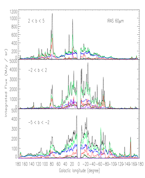
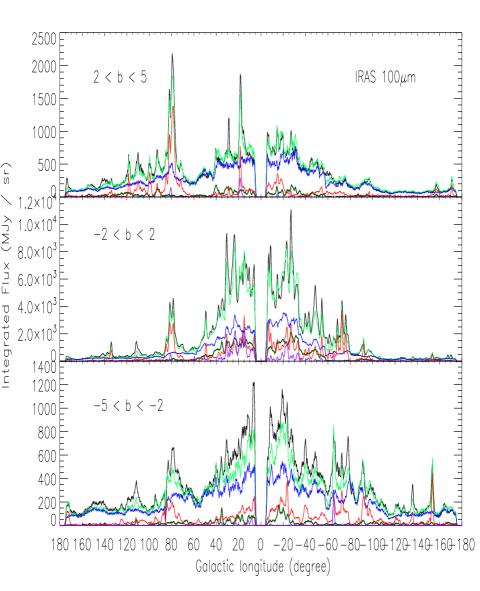
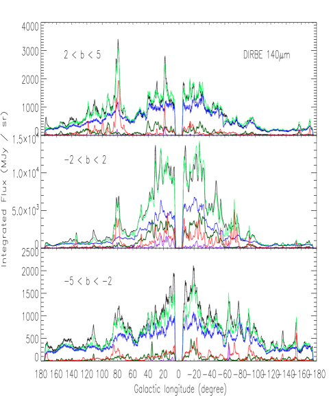
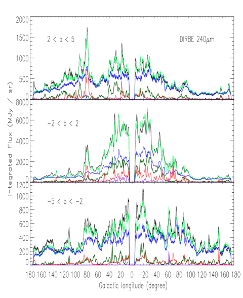
Figure 4: Longitude profiles for IRAS 60 and 100 $\mu$m (top panels) and DIRBE 140 and 240 $\mu$m (bottom panels). Black line denotes observed emission while light green line corresponds to the fitted model. In addition, blue line is for H_I, dark green line for H₂, red line for H${{}_{\sc{II}}}^{diffuse}$ and magenta line for H${{}_{\sc{II}}}^{compact}$. Profiles are obtained by averaging over the shown latitude intervals. The apparent noise is not instrumental: along the Galactic plane, the S/N is very high and error bars representing the instrumental noise would be of the same size of the plotting line.

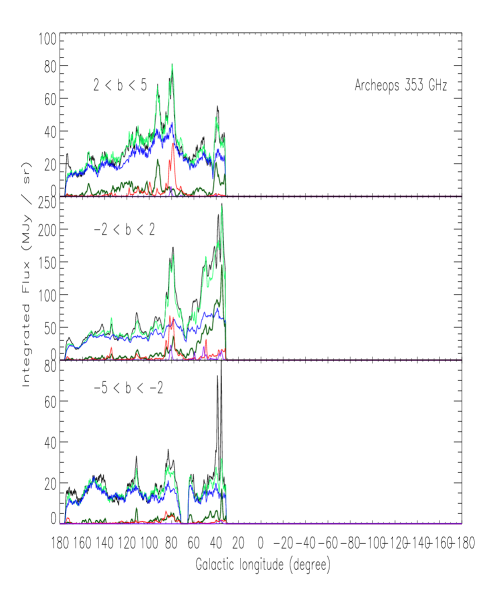
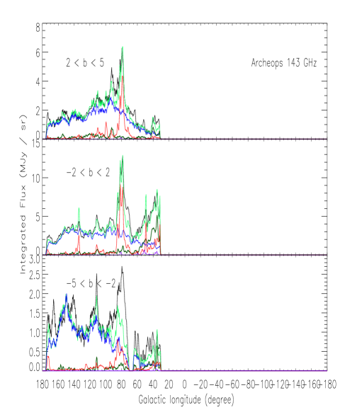
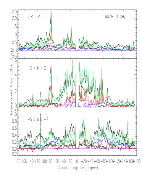
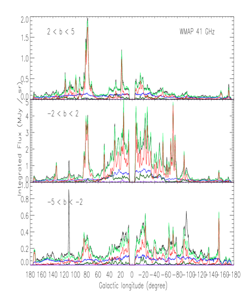
Figure 5: Longitude profiles for Archeops 850 and 2096 $\mu$m (top panels) and WMAP W and Q bands (bottom panels). Archeops data base covers only the longitude interval 30^∘ $<l<$ 180^∘. Black line denotes observed emission while light green line corresponds to the fitted model. In addition, blue line is for H_I, dark green line for H₂, red line for H${{}_{\sc{II}}}^{diffuse}$ and magenta line for H${{}_{\sc{II}}}^{compact}$. Profiles are obtained by averaging over the shown latitude intervals. The same remark as in Fig. 4 on instrumental noise applies here.

4 Derived physical parameters

4.1 The iterative inversion method

In matrix form, the minimization of eq. (2) is equivalent to solving the linear system:

$$(A^{t}\Pi A)\epsilon_{\lambda}=A^{t}\Pi I_{\lambda}$$ (10)

where A is a $(3n+1)\times N$ matrix of the type:

$$\left(\begin{array}[]{cccccccccc}N^{1,1}_{H_{I}}&..&N^{1,n}_{H_{I}}&2N^{1,1}_{H_{2}}&..&2N^{1,n}_{H_{2}}&N^{1,1,c}_{H{{}_{II}}}&..&N^{1,n,c}_{H{{}_{II}}}&N^{1,d}_{H{{}_{II}}}\\ :&&:&:&&:&:&&:&:\\ N^{N,1}_{H_{I}}&..&N^{N,n}_{H_{I}}&2N^{N,1}_{H_{2}}&..&2N^{N,n}_{H_{2}}&N^{N,1,c}_{H{{}_{II}}}&..&N^{N,n,c}_{H{{}_{II}}}&N^{N,d}_{H{{}_{II}}}\end{array}\right)$$

$n$ being the number of rings in the decomposition and $N$ the number of pixels. In the expression above, $N^{j,i,c}_{H{{}_{II}}}$ denotes the column density in pixel $j$ and ring $i$ for the source (or compact) component of the ionized gas, while $N^{j,d}_{H{{}_{II}}}$ is the corresponding column density for the diffuse component. $\Pi$ has dimension $N\times N$ and is given by:

$$\Pi=\left(\begin{array}[]{cccc}\frac{1}{{\sigma_{1}}^{2}}&0&...&0\\ 0&&&:\\ :&&&0\\ 0&...&0&\frac{1}{{\sigma_{N}}^{2}}\end{array}\right)$$

with $\sigma_{j}$ the pixel noise of the input map. In eq. (11), the correlation matrix $A^{t}\Pi A$ is symmetric and positive-defined which allows the linear system to be solved by means of a Cholesky inversion method (see, for instance, Golub $\&$ van Loan, 1989). The major difficulty is represented by a correct evaluation of the noise which is largely dominated by the uncertainty associated with the model. To circumvent such a problem, we have applied an iterative method. This consists of making an initial assumption about the (instrumental) noise, computing the corresponding solution and then using the noise derived from this partial solution to reiterate the process. A true estimate of the real noise is obtained when, by repeating this process several times, the system converges. Convergence is, on average, reached within 10 iterations. In the first iteration the (intrumental) noise per pixel is assumed to be given by:

$$\sigma^{1}_{j}=\sigma_{ini}+5\%I_{\lambda}(j)$$ (11)

where $\sigma_{ini}$ represents the average noise of the I_λ map at high latitudes and I_λ(j) is the value of the map in pixel $j$. In this expression, the term proportional to the observed signal is very important. The sky is in fact highly inhomogeneous and variations in signal in the range 1 to 10,000 (in brightness units) are observed when high latitutes are compared to low ones. It is then very unlikely that the difference between the true and the measured signal is only the same additive noise as it is at high Galactic latitudes. A proportional term taking into account the long term drift of the instrument gain needs to be considered. Nonetheless, it is important to emphasize that such definition of the noise is still rather crude and purely operational given the iterative method which has been adopted.
Emissivities coefficients obtained by following the procedure now described are shown in Table 2.

Gas phase	Ring	$\epsilon{{}_{\nu}}$     [MJy sr-1 (1020 H atoms cm-2)-1]
	(kpc)	60 $\mu$m	100 $\mu$m	140 $\mu$m	240 $\mu$m	850 $\mu$m	2096 $\mu$m
HI	0.1-4	3.9$\pm$0.08	13.7$\pm$0.89	26.4$\pm$0.68	12.46$\pm$0.27	—–	—-
	4-5.6	1.53$\pm$0.07	5.37$\pm$0.19	9.54$\pm$0.23	4.52$\pm$0.087	0.087$\pm$0.050	—-
	5.6-7.2	0.57$\pm$0.01	2.26$\pm$0.04	4.51$\pm$0.08	2.54$\pm$0.04	0.10$\pm$0.004	—-
	7.2-8.9	0.32$\pm$0.001	1.37$\pm$0.01	3.02$\pm$0.01	1.95$\pm$0.02	0.09$\pm$0.002	0.001$\pm$0.0002
	8.9-14	0.061$\pm$0.001	0.39$\pm$0.003	1.06$\pm$0.014	0.90$\pm$0.0046	0.091$\pm$0.0006	0.01$\pm$4.8e-05
	14-17	0.01$\pm$0.004	0.07$\pm$0.01	0.38$\pm$0.05	0.45$\pm$0.03	0.04$\pm$0.002	—-
H2	0.1-4	0.12$\pm$0.04	0.17$\pm$0.11	0.23$\pm$0.12	0.18$\pm$0.09	—-	—-
	4-5.6	0.20$\pm$0.01	0.74$\pm$0.04	1.45$\pm$0.05	0.75$\pm$0.04	0.05$\pm$0.007	0.001$\pm$0.0004
	5.6-7.2	0.14$\pm$0.01	0.63$\pm$0.02	1.72$\pm$0.03	1.10$\pm$0.04	0.051$\pm$0.006	0.00014$\pm$0.0003
	7.2-8.9	0.04$\pm$0.002	0.18$\pm$0.005	0.64$\pm$0.005	0.58$\pm$0.010	0.031$\pm$0.0005	0.001$\pm$8.4e-05
	8.9-14	0.03$\pm$0.001	0.15$\pm$0.004	0.47$\pm$0.02	0.42$\pm$0.014	0.02$\pm$0.001	0.001$\pm$0.0001
	14-17	0.009$\pm$0.004	—-	—-	0.0052$\pm$0.02	0.017$\pm$0.002	0.0026$\pm$0.0002
H${}_{II}^{compact}$	0.1-4	0.18$\pm$0.02	0.88$\pm$0.14	1.23$\pm$0.26	0.64$\pm$0.14	—-	—-
	4-5.6	2.44$\pm$0.24	5.93$\pm$0.29	4.22$\pm$0.43	1.52$\pm$0.32	—-	—-
	5.6-7.2	1.14$\pm$0.11	1.83$\pm$0.22	1.75$\pm$0.32	0.38$\pm$0.12	0.097$\pm$0.02	0.003$\pm$0.001
	7.2-8.9	3.49$\pm$0.31	6.81$\pm$0.68	10.17$\pm$1.45	4.77$\pm$1.1	0.26$\pm$0.06	0.005$\pm$0.001
	8.9-14	—-	—-	—-	—-	0.024$\pm$0.02	—-
	14-17	0.29$\pm$0.04	0.071$\pm$0.15	—-	—-	—-	—-
H${}_{II}^{diffuse}$	0.1-17	9.3$\pm$0.16	24.9$\pm$0.32	35.1$\pm$0.64	14.6$\pm$0.38	0.58$\pm$0.007	0.07$\pm$0.002

Table 2: Conversion factors to 4$\pi\nu\epsilon_{\nu}$ are, in units of 10^-31 W (H atom)^-1: 6.28, 3.77, 2.68, 1.57, 0.44, 0.18 at 60, 100, 140, 240, 850 and 2096 $\mu$m respectively. Quoted errors are derived as described in Section 4.

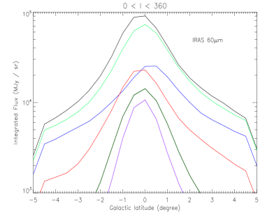
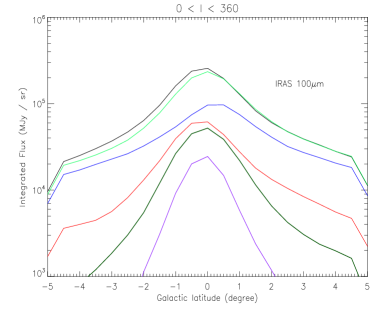
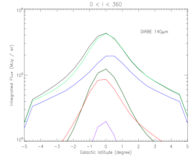
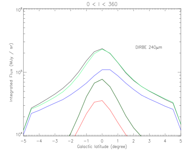
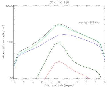
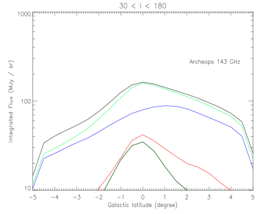
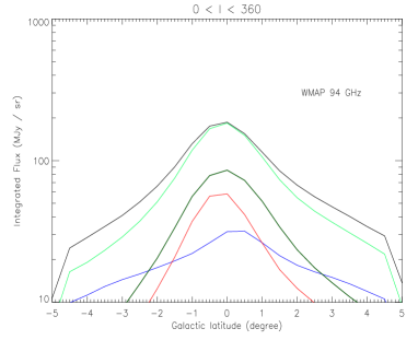
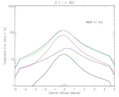
Figure 6: Latitude profiles (from top left, clockwise) for: IRAS 60 and 100 $\mu$m, DIRBE 140 and 240 $\mu$m, Archeops 850 and 2096 $\mu$m, WMAP W and Q bands. Black line denotes observed emission while light green line corresponds to the fitted model. In addition, blue line is for H_I, dark green line for H₂, red line for H${{}_{\sc{II}}}^{diffuse}$ and magenta line for H${{}_{\sc{II}}}^{compact}$.

Uncertainties quoted in the table have been computed by applying the bootstrap method described in Giard et al. (1994).

Figure 7: Galactocentric distributions of the infrared emissivities for dust associated with H_I (top left), H₂ (top right) and H${{}_{\sc{II}}}^{compact}$ (bottom center). Archeops results at 850 $\mu$m have been obtained for the longitude interval 30${}^{\circ}<$ l $<$ 180^∘.

4.2 Results and discussion

Fig. 4 and Fig. 5 show longitude profiles of the observed and modeled intensities as well as the respective contributions to the calculated profiles from H_I, H₂, diffuse H${{}_{\sc{II}}}^{diffuse}$ and H${{}_{\sc{II}}}^{compact}$. Fig. 6 illustrates the corresponding latitude profiles. The fitted region in the longitude profiles, at each frequency, covers the latitude range $|b|<$ 5^∘, due to the limited sky coverage of the CO observations. We also excluded the longitude range $|l|<$ 5^∘ and the corresponding region in the anticenter due to the lack of kinematic resolution in these directions. Although we could have corrected for this effect by, for instance, constraining the radial velocity interval, following the method implemented by Bertsch et al. (1993), we decided to ignore such a problem in the current analysis and to investigate the Galactic center region in detail in a forthcoming paper.

The longitude profiles show that the model fits are satisfactorily good at all wavelengths with the exception of a few peaks at 60 $\mu$m (which are not correctly reproduced) and some overshooting in the WMAP bands. The peaks are likely H_II regions and the model fails in this case because the H_II region catalog of Paladini et al. is complete only for fairly bright sources (see Section 3.4.2). In addition, as discussed in Section 3.4.2, the angular resolution of the WMAP free-free map does not allow one to resolve discrete sources. The overshooting testifies to an excess of emission and this can be explained by the fact that WMAP channels are mostly dominated by thermal bremstrahlung instead of dust emission (see also Fig. 8 and related discussion).

Similarly, the latitude profiles show that the model reproduces quite well the observed emission. Moreover, one can see that the emission between 60 and 2096 $\mu$m is dominated by dust associated with H_I although at 60 $\mu$m this is largely contributed by dust associated with the ionized gas. Remarkably, the H_II region contribution is clearly visible in the IRAS 60-$\mu$m profile but almost disappears in the corresponding plot for WMAP at 41 GHz despite the fact that the emission, at this wavelength, is mostly thermal radiation from the ionized gas. As discussed previously, this is an effect due to the angular resolution: IRAS resolving power matches the average angular size of cataloged H_II regions while WMAP resolution is 10 times lower.

Fig. 7 shows the Galactocentric distribution of dust emissivities associated with H_I, H₂ and H_II regions. The case of diffuse H_II is not plotted since for that component we do not have any 3d-spatial information. The emissivities for dust associated with H_I decreases strongly with increasing Galactocentric distance at all wavelengths with the exception of 850 $\mu$m which shows a less pronounced trend. Such behaviour appears both inside (R $<$ R_⊙) and outside (R $>$ R_⊙) the solar circle. On the contrary, the radial distribution for the emissivities of dust associated with H₂ shows a bump, at all $\lambda$, at R $\sim$ 5-6 kpc. Similarly, the distribution for dust associated with H_II regions presents a first pronounced bump at R $\sim$ 5 kpc and a second at R $\sim$ 8 kpc. In the case of H_I, if we combine this information with the fact that the intensity of the ISRF scales with Galactocentric distance in a comparable way (Mathis et al. 1983), we can conclude that dust mixed with atomic hydrogen is mostly heated by the general radiation field, in agreement with previous findings by Bloemen et al. (1990) and Sodroski et al. (1997). The behaviour of dust associated with molecular hydrogen suggests instead a correlation with the intense star formation activity taking place in the molecular ring, i.e. dust associated with H₂ appears to be heated also (and perhaps by a large fraction) by massive O and B stars still embedded in the parent molecular clouds rather by only the general radiation field . Sodroski et al. (1997) reached a similar conclusion while Blomen et al. (1990) did not find any significant correlation between the radial distribution of dust emissivity associated with H₂ and the molecular ring. As for H_II regions, the derived radial distribution of emissivities is fully consistent with the radial distribution of sources found in Paladini et al. (2004; see their Fig. 3).

The recovered emissivity coefficients allow one to compute the 60 $\mu$m/100 $\mu$m ratio in each Galactocentric bin, as shown in Table 3. The ratio is fairly constant for dust mixed with molecular gas with the exception of the first ring which is however characterized by a significant error. In the case of dust mixed with atomic gas though, we find a significant decreasing trend with Galactocentric radius although, within the solar circle (R $<$ 8.5 kpc), the gradient appears to be quite small. This second result partly contradicts Bloemen et al.’s finding that the 60 $\mu$m/100 $\mu$m ratio is nearly constant up to R $\sim$ 17 kpc. Nevertheless, when we take the mean values, we obtain 60 $\mu$m/100 $\mu$m ratios of $\sim$ 0.22 and 0.23 for, respectively, dust associated with atomic and molecular gas in agreement with Bloemen et al. (who report average values of $\sim$ 0.27 and 0.20) and also with typical values at high latitudes (for instance, Boulanger $\&$ Perault (1988) derive an average value of 0.21$\pm$0.02 at $|b|<$ 10 deg).

Gas phase	Ring	$\epsilon_{60\mu m}$/$\epsilon_{100\mu m}$
	(kpc)
HI	0.1-4	0.28$\pm$0.02
	4-5.6	0.28$\pm$0.01
	5.6-7.2	0.25$\pm$0.01
	7.2-8.9	0.23$\pm$0.002
	8.9-14	0.16$\pm$0.003
	14-17	0.14$\pm$0.06
H2	0.1-4	0.7$\pm$0.51
	4-5.6	0.27$\pm$0.02
	5.6-7.2	0.22$\pm$0.02
	7.2-8.9	0.22$\pm$0.01
	8.9-14	0.2$\pm$0.01
	14-17	—–

Table 3: 60 over 100 $\mu$m ratio for dust associated with H_I and H₂.

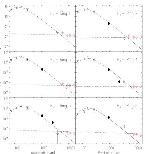
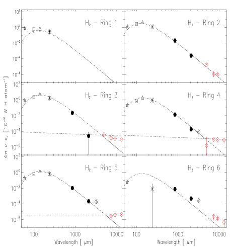
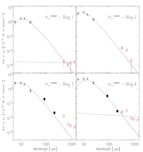
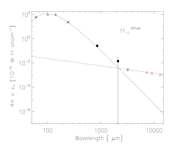
Figure 8: Derived emission spectra for dust associated with H_I (top left), H₂ (top right), H${{}_{\sc{II}}}^{compact}$ (bottom left) and H${{}_{\sc{II}}}^{diffuse}$ (bottom right). Dashed lines illustrates best-fitted modified black-body and power-law functions. Symbol notation is as in Fig. 7: the star corresponds to IRAS 60 $\mu$m, the square to IRAS 100 $\mu$m, the triangle to DIRBE 140 $\mu$m, the asterisk to DIRBE 240 $\mu$m, the filled circle to Archeops 850 $\mu$m and the black diamond to WMAP W-band. In addition, red diamonds denote WMAP K, Ka, Q and V bands.

The derived IR emission spectra for dust associated with each phase of the gas are shown in Fig. 8. We have fitted the FIR luminosity per H mass, $4\pi\nu\epsilon_{\nu}$ (in units of 10^-31 W (H ATOM)^-1), with a modified-blackbody, i.e.:

$$4\pi\nu\epsilon_{\nu}=4\pi\lambda\epsilon_{\lambda}=4\pi\lambda\alpha B_{T}(\lambda)\left(\frac{\lambda}{\lambda_{0}}\right)^{-\beta}$$ (12)

In this expression, $\alpha$ represents the dust cross-section per H atom (in units of m²/ H atom).

We have assumed a spectral emissivity index $\beta$ of 1.5. Such a value represents a compromise between the results obtained by Dupac et al. (2003) for M17, i.e. 1.3 $\leq\beta\leq$ 1.8 in the temperature range 35-15 K, and the fact that $\beta$=1.7 is usually adopted in the Solar neighborhood (Lagache et al. 2003). This flat spectral index is indicative of the existence of a millimeter excess with respect to the $\beta=2$ behavior expected from several grain models. Such an excess was observed for the first time in analyzing FIRAS data at $\lambda>$ 500 $\mu$m (Wright et al. 1991). A similar finding is also supported by observation of external galaxies as shown by Galliano et al. (2005). Finkbeiner et al. (1999) attribute this excess to a very low temperature (9 K) emission component in the diffuse ISM. Alternatively, the excess could be attributed to a temperature dependence of the dust submm emissivity spectral index (Meny et al. 2006)

By fitting the spectra with eq. (13), we derive estimates of the dust temperatures for every gas phase and for each radial interval (see Table 4). The following average temperatures have been obtained: T_d(H_I)=19.86$\pm$2.84 K, T_d(H₂)=19.23$\pm$2.18 K, T_d(H${{}_{\sc{II}}}^{diffuse}$)=26.7$\pm$0.1 K and T_d(H${{}_{\sc{II}}}^{compact}$)=27.87$\pm$2.89 K.

Clearly, the WMAP points (with the exception of W band) cannot be fitted by means of a modified black-body. Likely, this wavelength range is dominated by a mixture of thermal bremstrahlung (free-free), synchrotron emission and possibly (see Section 3.4) spinning dust rather than thermal radiation from stable dust in the diffuse ISM. This combination of radiative processes is not easy to model since the 3d-templates are not available and the synchroton spectral index varies spatially. Therefore, we fit the WMAP V to K bands with a power-law of the form $\alpha^{{}^{\prime}}$ $\lambda^{\beta^{{}^{\prime}}}$ where $\alpha^{{}^{\prime}}$ is a constant of normalization and $\beta^{{}^{\prime}}$ the spectral index for such a mixture of emission mechanisms. The power-law fit appears to represent satisfactorily the emissivity coefficients derived through the inversion technique. The best-fit $\alpha^{{}^{\prime}}$ and ${\beta^{{}^{\prime}}}$ values are shown in Table 4.

An additional interesting result of the fitting procedure is represented by the analysis of the Archeops point at 2096 $\mu$m as well as by the WMAP W-band value. In the outer Galaxy (Fig. 8, Ring 5 and 6) these points show a tendancy to lie above the fitted modified black body. This indicates that the galactic millimeter excess emission might be comparatively stronger towards the outer regions of the Galaxy. A similar finding was reported by Bourdin et al. (2002) also based on the use of the Archeops data. It is important to emphasize here that this result cannot be an artifact of our data analysis techniques. Such a spurious effect might be a matter of concern for the Archeops data set: the maps produced by the Trapani and Kiruna flights (Delabrouille, J. $\&$ Filliatre, P., 2004) have in fact been processed in a slightly different way, the Trapani map being significantly more filtered than the Kiruna map to correct for systematics. However, since such filtering affects the larger rather than the smaller scales, it would tend to decrease rather than increase the observed excess. At the same time, we point out that this result has been obtained by fixing $\beta$ to 1.5. A $\beta$ of 2 would enhance the excess even more.

The emissivity coefficients can also be combined with information on the mass distribution of the gas to compute FIR luminosities. In particular, if we denote with $i$ a given phase of the gas, the total FIR luminosity for this phase is obtained according to:

$$L_{FIR,i}=M_{i}\int_{\lambda_{min}}^{\lambda_{max}}{4\pi\lambda\epsilon_{i,\lambda}d\lambda}\hskip 51.21504pt[10^{8}L_{\odot}]$$ (13)

where M_i is the mass of the gas (expressed in 10⁸ M_⊙), 4$\pi\nu\epsilon_{\lambda}$ is the FIR luminosity per H mass (in L_⊙/M_⊙ units) and the integral is taken over the interval [$\lambda_{min}$,$\lambda_{max}$] = [60 $\mu$m, 2096 $\mu$m]. In writing eq. (14) we use again the fact that 4$\pi\nu\epsilon_{i,\nu}$ = 4$\pi\lambda\epsilon_{i,\lambda}$. As well as for the total Galaxy, FIR luminosities have been computed, for each phase of the gas, in each ring. In this case, the quantity M_i represents the mass of the gas in the considered Galactocentric interval. Masses for the atomic and molecular hydrogen have been derived by integrating, for each ring, the surface densities quoted by Binney $\&$ Merrifield (1998). As far as the ionized gas is concerned, we have made direct use of the estimate of the total mass reported by Westerhout (1958) for an effective electron density n_e=10 cm^-3. Remarkably, the value provided by Westerhout is a factor $\sim$ 40 lower than the one given in Ferriere (2001). The two values have been obtained in a different way: the Westerhout’s estimate is derived from free-free emission observations which are proportional to the emission measure (EM) while the Ferriere’s value is based on the Cordes et al. (1991) model which provides a direct measure of the electron column density (DM) (Katia Ferriere, private communication). The fact that our Galaxy contains several thermal components which are characterized by different clumping factors, i.e. different relations between DM and EM, explains the discrepancy in the two estimates.
The resulting FIR luminosities are given in Table 5.

Finally, we have computed the contribution of each component to the global SED. Fig. 9 shows that the dominant contribution at all wavelengths $>$ 60 $\mu$m is due to dust associated with atomic gas. However, at $\lambda$ $\sim$ 60 $\mu$m the emission is largely contributed by dust in H_II regions.

Gas phase	Ring	$\alpha$	T	$\alpha^{\prime}$	$\beta^{\prime}$
	(kpc)	(m2/ H atom)	(K)	(10-31 W H atom-1)
HI	0.1-4	0.01$\pm$0.0003	22.2$\pm$0.2	0.0005$\pm$9.0e-05	-0.12$\pm$0.002
	4-5.6	0.002$\pm$0.0002	22.9$\pm$0.5	4.1e-05$\pm$4.1e-06	0.05$\pm$0.03
	5.6-7.2	0.001$\pm$0.0004	21.1$\pm$1.01	3.9e-05$\pm$2.2e-07	-0.04$\pm$0.0003
	7.2-8.9	0.001$\pm$0.0005	19.8$\pm$1.4	1.5e-05$\pm$3.1e-07	0.02$\pm$ 0.003
	8.9-14	0.0008$\pm$0.0008	17.8$\pm$2.9	0.0001$\pm$5.2e-06	-0.17$\pm$0.0002
	14-17	0.0007$\pm$0.002	15.4$\pm$7.1	4.6e-05$\pm$1.6e-05	-0.16$\pm$ 0.002
H2	0.1-4	6.9e-05$\pm$0.0004	22.1$\pm$21.2	—-	—-
	4-5.6	0.0004$\pm$0.0003	21.7$\pm$3.2	0.0002$\pm$4.2e-05	-0.25$\pm$ 0.0002
	5.6-7.2	0.001$\pm$0.0007	18.7$\pm$2.4	0.0002$\pm$1.7e-05	-0.21$\pm$0.0002
	7.2-8.9	0.0007$\pm$0.001	16.9$\pm$5.2	7.3e-05$\pm$6.1e-06	-0.21$\pm$0.0002
	8.9-14	0.0004$\pm$0.001	17.4$\pm$7.2	—-	—-
	14-17	0.0002$\pm$0.03	18.6$\pm$222.0	—-	—-
H${{}_{\sc{II}}}^{compact}$	0.1-4	0.0002$\pm$0.0002	23.6$\pm$3.5	4.5e-06$\pm$3.9e-07	-0.06$\pm$0.003
	4-5.6	0.0005$\pm$3.8e-5	29.2$\pm$0.3	—-	—-
	5.6-7.2	1.5e-4$\pm$3e-5	30.0$\pm$0.8	—-	—-
	7.2-8.9	0.0007$\pm$6.1e-5	28.7$\pm$0.4	0.0012$\pm$2.2e-05	-0.21$\pm$0.001
	8.9-14	—-	—-
	14-17	—-	—-
H${{}_{\sc{II}}}^{diffuse}$	0.1-17	0.004$\pm$9.5e-5	26.7$\pm$0.1	0.36$\pm$0.003	-0.60$\pm$1.4e-08

Table 4: Derived temperatures for dust associated with each gas phase at increasing radial distance from the Galactic center.

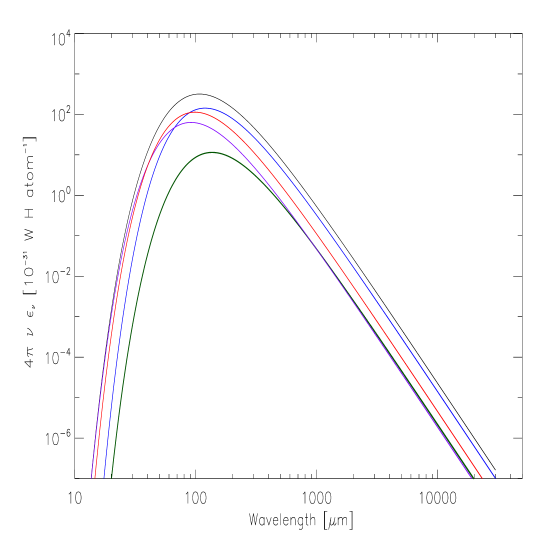
Figure 9: Global SED for our Galaxy obtained by summing up the contributions from dust associated with atomic, molecular and ionized gas (black solid line). $\alpha$ and $T$ parameters are from Table 4. Also shown are the individual emission components: dust in atomic (blue line), molecular (dark green line), diffuse ionized (red line) and compact ionized (magenta line).

Ring	${M_{HI}}^{a}$	$\frac{L_{FIR,H_{I}}}{M_{HI}}$	L${}_{FIR,H_{I}}$	${M_{H2}}^{a}$	$\frac{L_{FIR,H_{2}}}{M_{H2}}$	L${}_{FIR,H_{2}}$	${M_{HII}}^{diff,b}$	$\frac{L_{FIR,{HII}^{diff}}}{{M_{HII}}^{diff}}$	L${}_{FIR,{H_{II}}^{diff}}$
(kpc)	(108 M⊙)	(L⊙/M⊙)	(108 L⊙)	(108 M⊙)	(L⊙/M⊙)	(108 L⊙)	(108 M⊙)	(L⊙/M⊙)	(108 L⊙)
0.1-4	1.1	104.9	115.4	1.2	0.1	0.1
4-5.6	1.8	25.3	45.6	2.4	3.7	8.8
5.6-7.2	2.4	7.7	18.4	2.2	3.6	7.9
7.2-8.9	3.1	5.2	16.0	1.1	1.3	1.4
8.9-14	15.7	2.1	33.0	1.9	0.9	1.7
14-17	10.8	0.7	7.8	5.1	0.7	3.5
Total  Galaxy	34.8	—-	263.3	13.9	—-	23.5	0.42	64.9	27.2

Table 5: Emissivities per H mass (L_FIR,i/M_i) are computed from values of $\epsilon_{\nu}$ quoted in Table 2 by using the following conversion factors: 1.92 at 60 $\mu$m, 1.15 at 100 $\mu$m, 0.82 at 140 $\mu$m, 0.48 at 240 $\mu$m, 0.13 at 850 $\mu$m and 0.05 at 2096 $\mu$m.
^a Based on surface density diagram in Binney $\&$ Merrifield (1998).
^b From Westerhout (1958). Effective electron density n_eff = 10 cm^-3 .

5 Conclusions

By using an inversion technique, we have derived the radial distribution of dust properties in our Galaxy in the wavelength range 60 to 2096 $\mu$m. In particular, we have obtained emissivity coefficients for dust associated with atomic, molecular and ionized gas. By assuming a modified black-body with $\beta$=1.5, we estimate that average temperatures for dust uniformly mixed with H_I, H₂ and H_II are of order of 19.8, 19.2 and 26.7 K respectively. It is important to emphasize that the derivation, through inversion techniques, of dust emissivity coefficients associated with the molecular and ionized phases may be affected by a mutual contamination due to the spatial correlation that exists between these phases. In turn, such contamination would affect the derived physical quantities such as temperature. As noted by Sodroski et al. (1997), only the use of RRLs to trace the ionized gas phase would allow one to circumvent this problem. From the radial distribution of the emissivity coefficients associated with each gas phase, we find evidence that dust associated with the H_I is heated by the global ISRF. On the contrary, dust in molecular clouds appears to be heated in a significant way by young massive stars still embedded in their parent clouds. Our best-fitted spectra show an excess at Archeops 2096 $\mu$m and WMAP 94 GHz. Such an excess, also found in FIRAS data, can be interpreted as due to a very cold dust component in the diffuse ISM or to a temperature dependence of the spectral emissivity index at submm wavelengths. In addition, The long-wavelength ($\lambda\geq$ 4900 $\mu$m) ) part of the spectra for the H_I and H₂ associated dust components appears to be dominated by a mixture of thermal bremstrahlung, synchrotron emission and likely spinning dust. The possibility of a significant contribution due to spinning dust will be analyzed in a forthcoming paper by means of auxiliary data at even longer wavelengths ($\lambda>$ 13000 $\mu$m). As shown by recent studies (i.e. Watson et al., 2005), the peak of anomalous emission is expected to be at 15000 $\mu$m.
The derived emissivity coefficients also allow us to compute FIR luminosities. For these, the dominant contribution ($\sim$ 80$\%$) results to be provided by dust associated with atomic gas.

- (1) Benoit et al., 2002, Astropart. Phys., 17, 101
- (2) Bennett, C. L., Bay, M., Halpern, M., Hinshaw, G., Jackson, C., 2003, ApJ, 583, 1
- (3) Bennett, C. L., Hill, R. S., Hinshaw, G., Nolta, M. R., Odegard, N., Page, L., Spergel, D. N., Weiland, J. L., et al., 2003, ApJS, 148, 97
- (4) Bernard, J.P, Abergel, A., Ristorcelli, I., Pajot, F., Torre, J. P., et al., 1999, A&A, 347, 640
- (5) Bertsch, D. L., Dame, T. M., Fichtel, C. E., Hunter, S. D., Sreekumar, P., Stacy, J. G., Thaddeus, P., 1993, ApJ, 416, 587
- (6) Binney, J. & Merrifield, M., 1998, Galactic Astronomy, Princeton University Press, Princeton, New Jersey
- (7) Bloemen, J. B. G. M., Deul, E. R. & Thaddeus, P., 1990, A&A, 233, 437
- (8) Bloemen, J. B. G. M., Strong, A. W., Blitz, L., Cohen, R. S., Dame, T. M., et al., 1986, A&A, 154, 25
- (9) Boughn, S. P., Cheng, E. S., Cottingham, D. A., Fixsen, D. J., 1991, in AIP Conf. Proc. 222, After the First Three Minutes, ed. S. S. Holt, C. L. Bennett, V. Trimble, New York, p. 107
- (10) Boulanger, F. & Perault, M., 1988, 330, 964
- (11) Boulanger, F., Abergel, A., Bernard, J.-P., Burton, W. B., Desert, F.-X., Hartmann, D., Lagache, G., Puget, J.-L., 1996, A&A, 312, 256
- (12) Bourdin, H., Boulanger, F., Bernard, J. P., Lagache, G., 2002, Ap&SS, 281, 243
- (13) Cordes, J. M., Ryan, M., Weisberg, J. M., Frail, D. A., Spangler, S. R., 1991, Natur., 354, 121
- (14) Cordes, J. M. & Lazio, T. J. W., astro-ph/0207156
- (15) Cordes,J. M. & Lazio, T. J. W., astro-ph/0301598
- (16) Cox, P., Krugel, E., Mezger, P. G., 1986, A&A, 155, 380
- (17) Cox, P., Mezger, P. G., 1988, Comets to Cosmology, ed. A. Lawrence, Springer, Berlin, Heidelberg, New York, p. 97
- (18) Dame, T. M., Ungerechts, H., Cohen, R. S., deGeus, E. J., Grenier, I. A., may. J., Murphy, D. C., Nyman, L.-A., Thaddeus, P., 1987, ApJ, 322, 706
- (19) Dame, T. M., Hartmann, D., Thaddeus, P., 2001, ApJ, 547, 792
- (20) Delabrouille, J. Filliatre, P., 2004, ApSS, V. 290, Issue 1, p. 119
- (21) Desert, F.-X, Boulanger, F., Pujet, J. L., 1990, A&A, 237, 215
- (22) Dickey, J. M. Lockman, F. J., 1990, Annu. Rev. Astron. Astrophys., 28, 215
- (23) Dickinson, C., Davies, R. D., Davis, R. J., 2003, MNRAS, 341, 1057
- (24) Draine, B. T. & Lee, H. M., 1984, ApJ, 285, 89
- (25) Draine, B. T. & Anderson, N., 1985, ApJ, 292, 494
- (26) Draine, B. T. & Li, A., 2001, ApJ, 551, 807
- (27) Dupac, X., Giard, M., Bernard, J.-P., Lamarre, J.-M., M ny, C. et al., 2001, ApJ, 553, 604
- (28) Dupac, X., Bernard, J.-P., Boudet, N., Giard, M., Lamarre, J.-M. et al., 2003, A&A, 404, 11
- (29) Dwek, E., Arendt, R. G., Fixsen, D. J., Sodroski, T. J., Odegard, N., 1997, ApJ, 475, 565
- (30) Ferriere, K. M., 2001, RvMP, 73, 103
- (31) Fich, M., Blitz, L. Stark, A. A., 1989, ApJ, 342, 272
- (32) Finkbeiner, D. P., Davis, M. Schlegel, D. J., 1999, ApJ, 524, 867
- (33) Finkbeiner, D. P., 2003, ApJS, 146, 407
- (34) Finkbeiner, D. P., Langston, G. I. & Minter, A. H., 2004, ApJ, 617, 350
- (35) Fukui, Y., 1999, Science with the Atacama Large Millimeter Array (ALMA), Associated Universities Inc.
- (36) Galliano, F., Madden, S. C., Jones, A. P., Wilson, C. D., Bernard, J. P., 2005, A&A, 434, 867
- (37) Giard, M., Lamarre, J. M., Pajot, F. Serra, G., 1994, AA, 286, 203
- (38) Golub, G. H. van Loan, C. F., 1989, Matrix Computation, 2nd. ed., The John hopkins University Press
- (39) Gorski, K. M., Hivon, E. Wandelt, B. D., 1999, in Proceedings of the MPA/ESO Cosmology Conference Evolution of Large-Scale Structure, ed. A. J. Banday, R. S. Sheth L. Da Costa, 37
- (40) Hauser, M. G., 1993, back to the Galaxy, ed. S. S. Holt & F. Verter, New York AIP, AIP Proc., 278, 201
- (41) Haynes, R. F., Caswell, J. L. Simons, 1978, Austr. J. Phys. Suppl., 45, 1
- (42) Kerr, F. J., 1968, in Stars and Stellar Systems, Vol. 7, Nebulae and Interstellar Matter, ed. B. M. Middlehurst and L. H. Aller, University of Chicago Press, p. 574
- (43) Lagache, G., Haffner, L. M., Reynolds, R. J., Tufte, S. L., 2000, A&A, 354, 247
- (44) Lagache, G., A&A, 2003, 405, 813
- (45) Lebrun, F. et al., 1983, ApJ, 274, 231
- (46) Li, A. & Greenberg, J. M., 1997, A&A, 323, 566
- (47) Mathis, J. S., Rumpl, W., Nordsieck, K. H., 1977, ApJ, 217, 425
- (48) Mathis, J. S., Mezger, P. G., Panagia, N., 1983, AA, 128, 212
- (49) Meny, C., Gromov, V., Boudet, N., Bernard, J.P., Paradis, D., Nayral, C. 2006, submitted to A&A
- (50) Mezger, P. G., Mathis, J. S., & Panagia, 1982, A&A, 105, 372
- (51) Mitra, D., Berkhuijsen, E. M., Muller, P., 2003, How Does the Galaxy Work? A Galactic Tertulia with Don Cox and Ron Reynolds, ed. Alfaro, E. J., Perez, E., Franco, J., Astrophysics and Space Science Library, Published by Kluwer Academic Publishers, Dordrecht, The Netherlands, 2004, p.93
- (52) Miville-Deschenes, M.-A. & Lagache, G., 2005, APJSS, 157, 302
- (53) Neugebauer, G., et al., 1984, ApJ, 278, L1
- (54) Paladini, R., Burigana, C., Davies, R. D., Maino, D., Bersanelli, M., Cappellini, B., Platania, P., Smoot, G., 2003, A&A, 397, 213
- (55) Paladini, R., Davies, R. D., DeZotti, G., 2004, MNRAS, 347, 237
- (56) Paladini, R., De Zotti, G., Davies, R. D., Giard, M., 2005, MNRAS, 360, 1545
- (57) Perrot, C. A. & Grenier, I. A., 2003, A&A, 404, 519
- (58) Reach, W. T., Dwek, E., Fixsen, D. J., Hewagama, T., Mather, J. C., 1995, ApJ, 451, 188
- (59) Reynolds, R. J., 1991, The interstellar disk-halo connection in galaxies, IAUS, 144, 67
- (60) Schraml, J. & Mezger, P. G., 1969, ApJ, 156, 269
- (61) Sodroski, T. J., Dwek, E. & Hauser, M. G., 1989, 336, 762
- (62) Sodroski, T. J., Odegard, N., Arendt, R. G., et al., 1997, ApJ, 480, 173
- (63) Stepnik, B., Abergel, A., Bernard, J.-P., et al., 2001, ASPC, 243, 47
- (64) Watson, R. A., Rebolo, R., Rubino-Martin, J.A., et al., 2005, ApJ, 624, 89
- (65) Weiland, J. L., Blitz, L., Dwek, E., Hauser, M. G., Magnani, L., Rickard, L. J., 1986, ApJ, 306, 101
- (66) Westerhout, G., 1958, BAN, 14, 215
- (67) Wright, E. L., Mather, J. C., Bennett, C. L., et al., 1991, ApJ, 381, 200
- (68) Zubko, V., Dwek, E. Arendt, R. G., 2004, ApJS, 152, 211