Can we discern microlensed gravitational-wave signals from the signal of precessing compact binary mergers?

Abstract

Microlensed gravitational waves (GWs) are likely observable by recognizing the signature of interference caused by $\sim\!\mathcal{O}(10\textrm{--}100)~{}\textrm{ms}$ time delays between multiple lensed signals. However, the shape of the anticipated microlensed GW signals might be confused with the modulation appearing in the waveform of GWs from precessing compact binary mergers. Their morphological similarity may be an obstacle to template-based searches to correctly identifying the origin of observed GWs and it seamlessly raises a fundamental question, can we discern microlensed GW signals from the signal of precessing compact binary mergers? We discuss the feasibility of distinguishing those GWs via examining simulated GW signals with and without the presence of noise. We find that it is certainly possible if we compare signal-to-noise ratios (SNRs) computed with templates of different hypotheses for a given target signal. We show that proper parameter estimation for lensed GWs enables us to identify the targets of interest by focusing on a half number of assumptions for the target signal than the SNR-based test.

Introduction.—Like electromagnetic waves propagating in the universe, gravitational waves (GWs) can be gravitationally lensed by massive objects between the distant source and the observer [1, 2, 3, 4, 5, 6, 7, 8]. Consequently, for the gravitational lensing of GWs, it is possible to consider all known types of lensing configurations governed by not only the relative position of the source to the lens but also the size, shape, and distribution of the lens mass.

In this Letter, we focus on the microlensing of GWs (GW microlensing, hereafter) expected to occur with stellar objects of masses $\lesssim\!10^{5}M_{\odot}$ acting as the lens. In specific, if the time delay between multiple lensed GWs is $\sim\!\mathcal{O}(10\textrm{--}100)~{}\textrm{ms}$, the short time delays yield the waveforms of those lensed GWs to interfere with each other so that the interference pattern, also known as beating pattern, becomes a characteristic signature of GW microlensing. [15, 12, 11, 13] Therefore, we can anticipate that detecting microlensed GWs is achievable by recognizing beating patterns from GW signals.

On the other hand, the precessional motion of a compact binary system—originated by the misaligned component spins against the orbital angular momentum of the binary—can introduce amplitude modulation and phase shift to a GW signal not assuming precession (see Fig. 1, for example). In particular, at first glance at the example signals in the figure, the modulation induced by the precession (the second top panel), mainly shown in the inspiral phase corresponding to $t\!<\!0~{}\textrm{s}$, looks quite similar to the beating pattern of a microlensed GW signal (the third top panel).

The morphological similarity between the two different types of GWs may be an obstacle to template-based searches requiring appropriate assumptions on the intrinsic and extrinsic parameters of the source binary system. Therefore, their similarity seamlessly raises a fundamental question: can we discern microlensed GW signals from the signal of precessing compact binary mergers? To answer this question, we start by describing how we prepare the example signals in Fig. 1 for the sake of this work. We will designate each signal as a microlensed signal and a precessing signal shortly.

Preparation of GW signals of interest.—For the preparation of test signals of interest, we utilize PyCBC [16, 17, 18] and choose a state-of-the-art phenomenological waveform model, IMRPhenomXPHM [19], not only to incorporate the effect of multipole harmonic modes of GW signal but also to prepare both nonprecessing and precessing GW signals in the same manner with and without the parameters for the precessing binary.

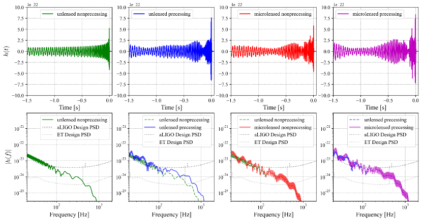
Figure 1: Example noise-free GW signals studied in this Letter. The top and bottom panels show signals in the time domain and the frequency domain, respectively. From the left to the right, each column shows the case of unlensed nonprecessing, unlensed precessing, microlensed nonprecessing, and microlensed precessing signals, respectively. The time of $h(t)$ is given with respect to the merging time at $t=0~{}\textrm{s}$. In the plots of $|h(f)|$, we display a counter example signal (dashed line) and the sensitivity curves of the Advanced LIGO (aLIGO)’s design power spectral density (PSD) (dotted dark grey) and the Einstein Telescope (ET)’s design PSD [20] (dotted light grey) for comparison.

First, we generate unlensed signals of nonprecessing binary and precessing binary ($h_{\textrm{N}}$ and $h_{\textrm{P}}$, respectively) with the common and precessing parameters summarized in Table 1. Note that the spin parameters are randomly chosen but to satisfy the spin magnitude $s\!=\!(s_{x}^{2}\!+\!s_{y}^{2}\!+\!s_{z}^{2})^{1/2}\!\leq\!1$.

Table 1: Parameters used for the generation of test signals of interest.

Case	Parameter	Value
Common	Mass 1, $m_{1}$	$30M_{\odot}$
	Mass 2, $m_{2}$	$10M_{\odot}$
	Luminosity distance, $d_{L}$	$500~{}\textrm{Mpc}$
	Inclination angle, $\iota$	$80~{}\textrm{deg}$
	Sampling rate	$8192~{}\textrm{Hz}$
Precessing	Spin 1, $\vec{s}_{1}\!=\!(s_{1x},s_{1y},s_{1z})$	(0.76, 0.06, 0.55)
	Spin 2, $\vec{s}_{2}\!=\!(s_{2x},s_{2y},s_{2z})$	(-0.19, 0.74, -0.33)
	Angle between total angular	$160~{}\textrm{deg}$
	momentum and line of sight, $\theta_{JN}$
Microlensed	Source position, $y$	0.9
	Log-redshifted lens mass,	$3.2$
	$\log_{10}\!(M_{lz}/M_{\odot})$

Following the choice, the effective precession spin parameter $\chi_{p}$ [21] of the precessing binary can be calculated as $\chi_{p}\!\simeq\!0.76$ via the chi_p function of PyCBC with the given component masses and the $x$- and $y$-components of component spins.

Next, we simulate a microlensed signal $h_{\textrm{ML}}$ via $h_{\textrm{ML}}(f)\!=\!F(f)h(f)$ adopting the thin-lens approximation, where $h(f)$ in the right-hand side denotes an unlensed signal, either $h_{\textrm{N}}$ or $h_{\textrm{P}}$, given in the frequency domain and $F(f)$ is the amplification factor given as a function of frequency $f$. To specify $F(f)$ enabling us to simulate a $h_{\textrm{ML}}(f)$ in a simple means, we take the point-mass lens model in the geometrical optics limit which makes $F(f)$ can be written as

$$F(f)=\sqrt{|\mu_{+}|}\!-\!i\sqrt{|\mu_{-}|}e^{2\pi if\Delta t}~{},$$ (1)

where $\mu_{+}$ and $\mu_{-}$ are the magnification factor for each of the two lensed signals and $\Delta t$ is the time delay between them: $\mu_{\pm}$ and $\Delta t$ are given as

$$\mu_{\pm}=\frac{1}{2}\pm\frac{y^{2}+2}{2y\sqrt{y^{2}+4}}~{},$$ (2)

and

$$\Delta t=\frac{4GM_{lz}}{c^{3}}\left[\frac{y\sqrt{y^{2}+4}}{2}+\ln\left\{\frac{\sqrt{y^{2}+4}+y}{\sqrt{y^{2}+4}-y}\right\}\right]~{},$$ (3)

respectively, where $y$ is a dimensionless parameter for the source position and $M_{lz}\!=\!M_{l}(1+z)$ is the redshifted lens mass.

We then convert the signals in the frequency domain to the time domain via the inverse Fourier transformation. Note that we empirically choose $y=0.9$ and $M_{lz}=10^{3.2}M_{\odot}$ in order to make an apparently similar $h_{\textrm{ML}}(t)$ to given $h_{\textrm{P}}(t)$; the parameters give $\mu_{+}\simeq 1.21$, $\mu_{-}\simeq-0.21$, and $\Delta t\simeq 58~{}\textrm{ms}$.

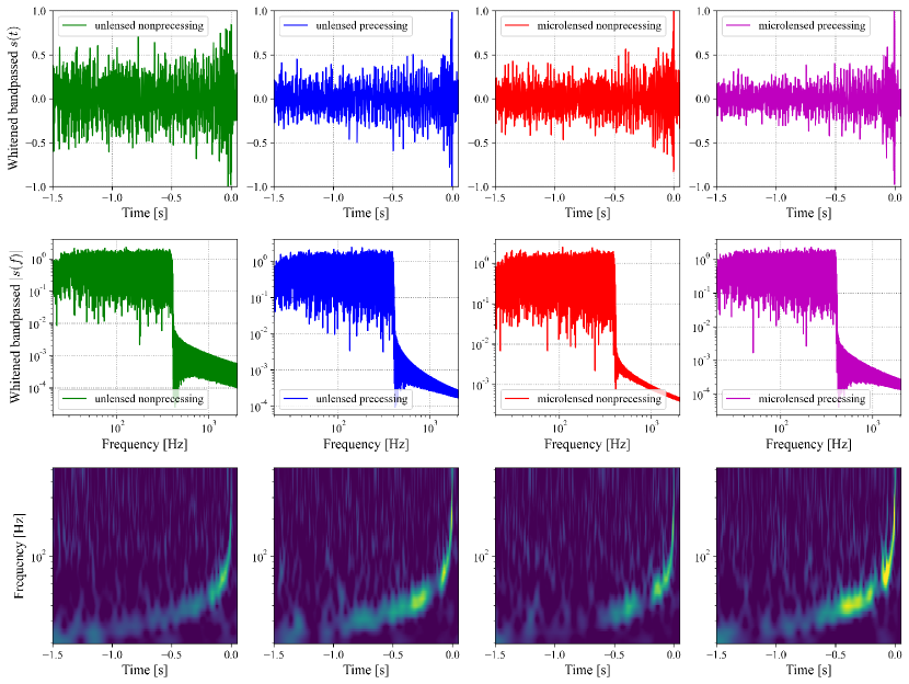
Figure 2: The same signals of Fig. 1 but injected into the noise data of the PSD of aLIGO’s design sensitivity. For visual convenience, we plot whitened signals for both bandpassed $s(t)$ and $|s(f)|$. We further normalize $s(t)$ with the peak amplitude at $t=0~{}\textrm{s}$. We also present the spectrogram of each signal in the bottom panel.

Finally, regarding realistic detection scenario, we inject the time-domain signals into the noise data $n(t)$ to simulate the strain data $s(t)$ such as $s(t)\!=\!h(t)\!+\!n(t)$. For $n(t)$, we consider a noise model, the power spectral density (PSD) of the Advanced LIGO (aLIGO)’s design sensitivity [22], that also can be acquired from the pycbc.psd module of PyCBC. In addition, to obtain the final form of $s(t)$, we employ bandpass filtering following the conventional signal processing for the LIGO-Virgo data [23]: For our example signals, we apply an empirically determined optimal frequency window $[20\textrm{Hz},400\textrm{Hz}]$ for the bandpass filter. We present the resultant $s(t)$ and $|s(f)|$ in the top and middle panels of Fig. 2, respectively.

Comparison between signals in noise.—Let us discuss the feasibility of distinguishing signals of interest by comparing the signals in given noise. Hereafter, ‘un’, ‘up’, ‘ln’, and ‘lp’ stand for the unlensed nonprecessing, unlensed precessing, (micro)lensed nonprecessing, and (micro)lensed precessing signals, respectively.

We can see from Fig. 2 that the presence of noise obviously hinders recognizing the difference between signals shown in the noise-free $h(t)$ or $|h(f)|$. The difficulty in identifying the difference is also shown in the spectrogram presented in the bottom panel of Fig. 2: We can find that the brightness—representing the energy content of the signal [24]—of the ‘un’ signal (the first panel) changes like the ‘up’ signal (the second panel) as the time and frequency evolve. We also observe a few faint vertical nodes appear on both signals.

From the spectrograms of ‘ln’ and ‘lp’ signals (the third and fourth panels, respectively), we can still see some brightness changes for $t<-0.1~{}\textrm{s}$ similar to ‘un’ and ‘up’ signals. However, we can observe two peaks, the primary peak at $t=0~{}\textrm{s}$ and the secondary peak at $t\sim-0.06~{}\textrm{s}$, which well agree with $\Delta t\simeq 58~{}\textrm{ms}$ but not shown in the spectrograms of ‘un’ and ‘up’. Despite this, this makes us to hardly identify whether a microlensed signal is a precessing signal or a nonprecessing signal. On top of that, the only recognizable differences between the third and fourth spectrograms are the amount of brightness and apparent visibility of two peaks or the presence of a dark vertical node at slightly different times, i.e., $t\!\sim\!-0.2~{}\textrm{s}$ for ’ln’ and at $t\!\sim\!-0.15~{}\textrm{s}$ for ‘lp’; these differences do not tell us about the original intrinsic property of a microlensed signal.

Table 2: Matched-filter signal-to-noise ratios (SNR) of noisy signals corresponding to the examined pairs of template and target. We also tabulate the noise-free cases for comparison. For the computation of SNR of noise-free targets, we use the PSD of aLIGO’s design sensitivity. We find that SNRs of homogeneous pairs are advantageous for obtaining higher SNRs than heterogeneous pairs as expected. We also see SNRs of precessing targets are slightly higher than nonprecessing targets.

Noise	Homogeneous BBH pairs (template-target)						Heterogeneous BBH pairs (template-target)
	Nonprecessing target			Precessing target			Nonprecessing target			Precessing target
	un–un	un–ln	ln–ln	up–up	up–lp	lp–lp	up–un	up–ln	lp–ln	un–up	un–lp	ln–lp
Free	$24.5$	$27.2$	$29.4$	$35.6$	$39.5$	$42.7$	$8.5$	$10.9$	$11.2$	$12.3$	$14.0$	$16.3$
aLIGO	$24.3$	$26.4$	$28.4$	$34.0$	$36.4$	$40.1$	$9.6$	$12.2$	$4.8$	$13.0$	$14.1$	$4.9$

To quantitatively examine the distinguishability, we compute matched-filter signal-to-noise ratio (SNR) and summarize resulting SNRs in Table 2. For this examination, we configure multiple template-target pairs with the four-types signals studied thus far: We take whitened noise-free signals as templates and whitened noisy signals as targets. We classify the pairs into two categories, homogeneous BBH pairs and heterogeneous BBH pairs, defining homogeneous or heterogenous to represent whether the same nonprecessing/precessing binary system is supposed for both template and target or not: Following the definition, ‘xn-xn’ and ‘xp-xp’ correspond to homogeneous pairs and ‘xn-xp’ and ‘xp-xn’ correspond to heterogeneous pairs regardless of ‘x’, where ‘x’ can be either ‘u’ or ‘l’. We then collect each pair of the two categories into two additional subcategories of nonprecessing or precessing target signals.

From the SNRs of homogeneous BBH pairs, we see that SNRs for precessing targets are commonly $\sim\!40\%$ higher than corresponding SNRs for nonprecessing targets. We observe that testing mirolensed templates for microlensed targets shows the highest SNR among the pairs of each subcategory. We also find that unlensed templates are applicable even for microlensed targets because SNRs of ‘un-ln’ and ‘up-lp’ are higher than SNRs of unlensed targets.

Obtaining higher SNR for precessing target is still shown from the SNRs of heterogeneous BBH pairs. However, when we compare SNRs of heterogeneous BBH pairs to corresponding homogeneous pairs for the same target, we can see that using heterogeneous templates to opposite targets gives much lower SNRs. In particular, as shown from ‘lp-ln’ and ‘ln-lp’ pairs in aLIGO noise, computing SNR with heterogeneous microlensed template is obviously disadvantageous for finding microlensed targets because it is much lower than the detection criterion $\geq 8$ for the matched-filter SNR of a single detector [25].

The result of this SNR-based test provides an answer for our question: It is feasible to distinguish a microlensed nonprecessing signal from an unlensed precessing signal if an adequate homogeneous template is tested and higher SNR is obtained than other templates. For example, for ‘ln’ target, we obtain SNRs as $28.4$, $26.4$, and $12.2$ with ‘ln’, ‘un’, and ‘up’ templates, respectively. Similarly, we get SNRs for ‘up’ target as $34.0$ and $13.0$ with ‘up’ and ‘un’ templates, respectively. Moreover, we find discriminating a microlensed nonprecessing target from a microlensed precessing target is also possible when we compare SNRs of ‘ln’ and ‘lp’ targets, e.g., ‘ln-ln’ ($28.4$) and ‘lp-ln’ ($4.8$) or ‘lp-lp’ ($40.1$) and ‘ln-lp’ ($4.9$).

In practice, the analysis methods using templates (e.g., PyCBC and GstLAL [26]) are the de facto standard for searching GWs from compact binary mergers. Therefore, our results suggest that utilizing the standard methods with an adequate template bank consisting of microlensed waveforms including precession will be a promising approach for determining if a GW event is microlensed or not.

On the other hand, the results also imply that, to distinguish the target of interest, we have to repeat computing SNR multiple times regarding all possible hypotheses for the nature of a single target. However, since the template-based searches require hundreds thousands of template waveforms, e.g., $\sim\!\textrm{250,000}$ templates for GW150914 [27], demanding such repeated computation will inevitably increase the total computation time of our test at least $\mathcal{N}$ times more, where $\mathcal{N}$ is the number of hypotheses. For example, if we want to identify whether a target is an unlensed/microlensed nonprecessing/precessing signal, we have to test the four hypotheses, ‘un’, ‘up’, ‘ln’, and ‘lp’ and repeat the same analysis of finding a template giving the highest SNR for each hypothesis. Then, the whole procedure for finally picking up the most promising template from four of them will take at least $4\times$ more computation time in total compared to the typical search for a single BBH signal.

Parameter estimation for microlensed signals.—We conduct parameter estimation (PE) to demonstrate whether a proper PE can help us to disclose the origin of a given target. In particular, we focus on ‘ln’ and ‘lp’ signals because the apparent similarity—showing the modulation in waveform and double peaks around the merging time—between them makes us hardly identify their intrinsic origin.

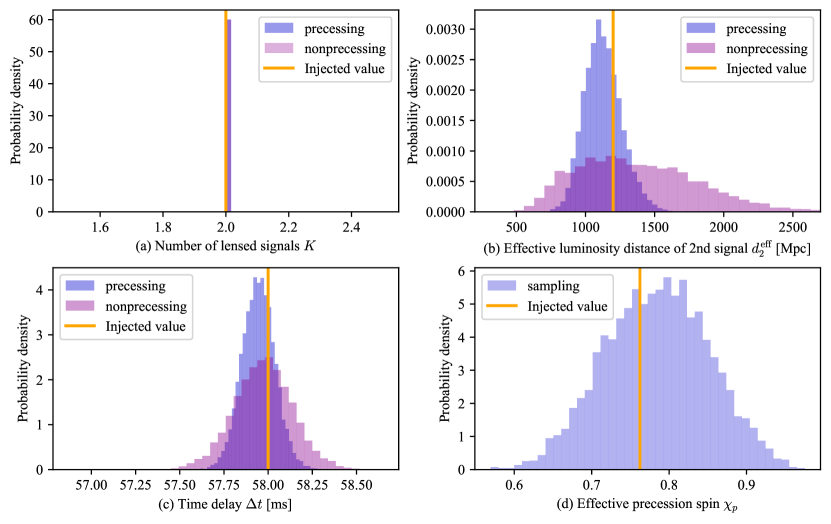
Figure 3: Posterior probability density functions (PDFs) of the parameter (a) $K$, (b) $d_{2}^{\mathrm{eff}}$, (c) $\Delta t$, and (d) $\chi_{p}$. The precessing and nonprecessing signals lead to consistent results with the injected values (orange lines). Note that, for $\chi_{\textrm{P}}$, we present the posterior PDF of precessing signal only because $\chi_{p}\!=\!0$ for nonprecessing signals [21].

The PE method [14] implemented in this work is based on a phenomenological lensed waveform model with specifically rewriting $F(f)$ in a parametric form such as

$$F(f,d^{\textrm{eff}}_{j},t_{j},n_{j})=\sum_{j=1}^{K}\frac{d_{L}}{d_{j}^{\textrm{eff}}}e^{2\pi ft_{j}-i\pi n_{j}}~{},$$ (4)

where $K$ refers to the number of lensed signals and $d^{\textrm{eff}}_{j}\equiv d_{L}/\sqrt{\mu_{\textrm{rel},j}}$ is the effective luminosity distance of $j^{\textrm{th}}$ lensed signal for the given true luminosity distance to the source $d_{L}$. $\mu_{\textrm{rel},j}\!\equiv\!|\mu_{j}/\mu_{1}|$ and $t_{j}$ are respectively defined as the relative magnification and the relative time delay of $j^{\textrm{th}}$ signal with respect to the first lensed signal. $n_{j}$ denotes the Morse phase index [28] of $j^{\textrm{th}}$ signal. The advantage of using the parameterized $F(f,d^{\textrm{eff}}_{j},t_{j},n_{j})$ is that we can determine $F$ for an arbitrary number of individual lensed signal with the relative lensing observables without specifying the observables such as $y$ and $M_{lz}$. We can then write the $h_{\textrm{ML}}$ as the superposition of multiple lensed GW signals such as

$$h_{\textrm{ML}}(f)=\left(\sum_{j=1}^{K}\frac{d_{L}}{d^{\mathrm{eff}}_{j}}e^{2\pi ift_{j}-i\pi n_{j}}\right)h(f)~{}.$$ (5)

Consequently, depending on the result of inferred $K$, we can determine whether the analyzed GW signal is multiply lensed or not. Note that $K\!=\!2$ for the case of a point-mass lens, so that $j\!=\!1,2$ leading $n_{j}$ becomes $n_{1}\!=\!0$ and $n_{2}\!=\!0.5$ for the first and second lensed signals, respectively.

For this PE, we prepare another two target strain data—injecting the same $h_{\textrm{ln}}$ and $h_{\textrm{lp}}$ into the Gaussian noise of the aLIGO’s design sensitivity PSD using a Bayesian inference library, bilby [31, 32]—and infer the lensing parameters together with the source parameters. In computing the likelihood, we adopt the nested sampling technique with pymultinest sampler [33, 34] and use two waveform models, IMRPhenomXHM [35] and IMRPhenomXPHM, for the template of nonprecessing and precessing targets, respectively. In Fig. 3, we present resulting probability density functions (PDFs) of the posteriors of 4 selected parameters, $K$, $d^{\textrm{eff}}_{2}$, $\Delta t$, and $\chi_{p}$, where $\Delta t\!\equiv\!t_{2}$.

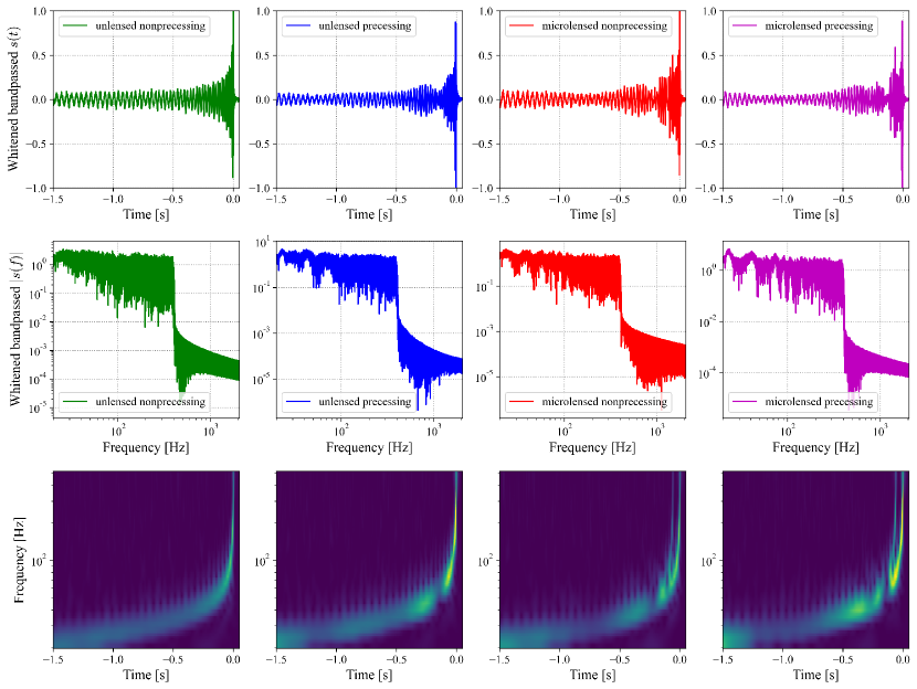
Figure 4: The same signals shown in Fig. 1 but injected into the noise data of the PSD of ET’s design sensitivity.

We find that our PE correctly recovers the number of lensed signals $K$ as $2$ for both ‘ln’ and ‘lp’ signals (see Fig. 3(a)). From this result, we confirm that precession does not affect identifying microlensed events. We also see that, for both precessing and nonprecessing cases, the resulting posteriors of $d^{\textrm{eff}}_{2}$ and $\Delta t$ include the injected values, i.e., $d^{\textrm{eff}}_{2}\!\simeq\!1200~{}\textrm{Mpc}$ and $\Delta t\simeq 58~{}\textrm{ms}$ (see Fig. 3(b) and Fig. 3(c), respectively) within their distributions. On top of that, since we can recover $\chi_{p}$ from the microlensed precessing signal in agreement with the injected value $\sim 0.76$ (Fig. 3(d)), our PE helps us to identify a precessing signal correctly.

When we compare the precessing and nonprecessing cases of $d^{\textrm{eff}}_{2}$ and $\Delta t$, we can observe the range of posterior distribution for precessing signal is narrower than that for nonprecessing one. For this observation, we presume the performance of our PE is sensitive to SNR because it turned out that the SNRs of those two signals calculated during PE are $\textrm{SNR}_{\textrm{lp-lp}}=30.5>\textrm{SNR}_{\textrm{ln-ln}}=15.6$.

We conclude that the PE-based analysis can inform us about whether a target signal is microlensed or not (via $K$) and whether the correctly identified microlensed signals is from a nonprecessing or a precessing binary (via $\chi_{p}$). Moreover, for the identification of the targets of interest, we find the PE-based analysis is more beneficial than the SNR-based test in practice because, by recovering $K$, we can focus on two hypotheses related to the precession only without further estimation on the other two hypotheses associated with the microlensing.

Discussions.—In this Letter, we have supposed the GW microlensing occurs with a point-like lens mass of $M_{lz}\!=\!10^{3.2}M_{\odot}$ in the geometrical optics limit for simplicity. However, if we consider (i) extended lens mass, e.g., singular isothermal sphere, in quasi-geometrical optics approximation [36] or (ii) more complex microlensing configurations in wave optics, e.g., studied in [15, 12], we expect more than two lensed signals which may introduce more complex beating patterns on GW signals. Therefore, debating the distinguishability in more realistic microlensing scenarios with such treatments/configurations will be worth to devote.

On the other hand, when we look at the same signals but injected into the noise model of ET’s design sensitivity [20] (see Fig. 4), the identification becomes obviously much easier than the case of aLIGO’s noise. Indeed, we can see quite similar shaped signals from the whitened bandpassed $s(t)$s compared to the shape seen in the corresponding noise-free $h(t)$s in Fig. 1. Additionally, from the spectrogram, we can observe a similar pattern in the signals corresponding to the signals in Fig. 2 but much clearer ones, although distinguishing nonprecessing and precessing signals from the microlensed cases is still quite hard because both signals are amplified and have double peaks near the merger time. Despite this, if a proper PE-based analysis will be accompanied with the identification of microlensed event as done in this work, it will be definitely possible to recognize whether the microlensed event is from a precessing or nonprecessing binary.

In principle, one could do more comprehensive studies such as a systematic study for various physical and lensing parameters as done in [37]. However, our results have demonstrated already that the precessional effect is not degenerate with beating patterns and have shown that the signals of interest are distinguishable with both SNR- and PE-based tests. For the result, we presume that the methods adopted in our tests are good enough at capturing the difference between the intrinsic effect introducing the modulation in precessing signals and the extrinsic effect resulting in the interference of multiple lensed signals. Nonetheless, finding a decisive criterion for the discrimination will be helpful for future observations on GWs containing various intrinsic/extrinsic natures. For example, it is also known that another intrinsic degree of freedom, the eccentricity, of a compact binary merger can introduce modulation in GW waveforms (see Figure 1 of [38], for example) and it makes us confused in identifying whether the modulation is caused by precessing or eccentric binaries [39, 40, 41]. Thus, exploring the distinguishability between the beating pattern of microlensed GWs and other modulations originated by diverse intrinsic properties of compact binary systems will be another interesting venue.

Acknowledgements.—The authors thank Otto A. Hannuksela, Tjonnie G. F. Li, and Eungwang Seo for fruitful discussions and comments. This work is supported by the National Research Foundation of Korea (NRF) grant funded by the Ministry of Science and ICT of the Korea Government (NRF-2020R1C1C1005863). K.K. also acknowledges that the computational work reported in this Letter was partly performed on the KASI Science Cloud platform supported by Korea Astronomy and Space Science Institute.

References

- Ohanian [1974] H. C. Ohanian, On the focusing of gravitational radiation, Int. J. Theor. Phys. 9, 425 (1974).
- Bliokh and Minakov [1975] P. V. Bliokh and A. A. Minakov, Diffraction of light and lens effect of the stellar gravitation field, Ap&SS 34, L7 (1975).
- Bontz and Haugan [1981] R. J. Bontz and M. P. Haugan, A diffraction limit on the gravitational lens effect, Ap&SS 78, 199 (1981).
- Thorne [1983] K. S. Thorne, The theory of gravitational radiation: An introductory review, in Gravitational Radiation, edited by N. Deruelle and T. Piran (Amsterdam: North Holland, 1983).
- Deguchi and Watson [1986] S. Deguchi and W. D. Watson, Diffraction in gravitational lensing for compact objects of low mass, Astrophys. J. 307, 30 (1986).
- Schneider et al. [1992] P. Schneider, J. Ehlers, and E. E. Falco, Gravitational Lenses (Springer, New York, 1992) p. 112.
- Nakamura and Deguchi [1999] T. T. Nakamura and S. Deguchi, Wave Optics in Gravitational Lensing, Prog. Theor. Phys. Suppl. 133, 137 (1999).
- Takahashi and Nakamura [2003] R. Takahashi and T. Nakamura, Wave effects in gravitational lensing of gravitational waves from chirping binaries, Astrophys. J. 595, 1039 (2003), arXiv:astro-ph/0305055 .
- Hannuksela et al. [2019] O. Hannuksela, K. Haris, K. Ng, S. Kumar, A. Mehta, D. Keitel, T. Li, and P. Ajith, Search for gravitational lensing signatures in LIGO-Virgo binary black hole events, Astrophys. J. Lett. 874, L2 (2019), arXiv:1901.02674 [gr-qc] .
- Abbott et al. [2021] R. Abbott et al. (LIGO Scientific, VIRGO), Search for Lensing Signatures in the Gravitational-Wave Observations from the First Half of LIGO–Virgo’s Third Observing Run, Astrophys. J. 923, 14 (2021), arXiv:2105.06384 [gr-qc] .
- Kim et al. [2021] K. Kim, J. Lee, R. S. H. Yuen, O. A. Hannuksela, and T. G. F. Li, Identification of Lensed Gravitational Waves with Deep Learning, Astrophys. J. 915, 119 (2021), arXiv:2010.12093 [gr-qc] .
- Seo et al. [2022] E. Seo, O. A. Hannuksela, and T. G. F. Li, Improving Detection of Gravitational-wave Microlensing Using Repeated Signals Induced by Strong Lensing, Astrophys. J. 932, 50 (2022).
- Kim et al. [2022] K. Kim, J. Lee, O. A. Hannuksela, and T. G. F. Li, Deep Learning–based Search for Microlensing Signature from Binary Black Hole Events in GWTC-1 and -2, Astrophys. J. 938, 157 (2022), arXiv:2206.08234 [gr-qc] .
- Liu et al. [2023] A. Liu, C.-F. Wong, S. Leong, A. More, O. Hannuksela, and T. Li, A phenomenological description of gravitational-wave millilensing (2023), LIGO-P2200365.
- Diego et al. [2019] J. Diego, O. Hannuksela, P. Kelly, T. Broadhurst, K. Kim, T. Li, G. Smoot, and G. Pagano, Observational signatures of microlensing in gravitational waves at LIGO/Virgo frequencies, Astron. Astrophys. 627, A130 (2019), arXiv:1903.04513 [astro-ph.CO] .
- Dal Canton et al. [2014] T. Dal Canton et al., Implementing a search for aligned-spin neutron star-black hole systems with advanced ground based gravitational wave detectors, Phys. Rev. D 90, 082004 (2014), arXiv:1405.6731 [gr-qc] .
- Usman et al. [2016] S. A. Usman et al., The PyCBC search for gravitational waves from compact binary coalescence, Class. Quant. Grav. 33, 215004 (2016), arXiv:1508.02357 [gr-qc] .
- Nitz et al. [2020] A. Nitz, I. Harry, D. Brown, et al., gwastro/pycbc: Pycbc release v1.16.11 (2020).
- Pratten et al. [2021] G. Pratten et al., Computationally efficient models for the dominant and subdominant harmonic modes of precessing binary black holes, Phys. Rev. D 103, 104056 (2021), arXiv:2004.06503 [gr-qc] .
- Hild et al. [2011] S. Hild et al., Sensitivity Studies for Third-Generation Gravitational Wave Observatories, Class. Quant. Grav. 28, 094013 (2011), arXiv:1012.0908 [gr-qc] .
- Schmidt et al. [2015] P. Schmidt, F. Ohme, and M. Hannam, Towards models of gravitational waveforms from generic binaries II: Modelling precession effects with a single effective precession parameter, Phys. Rev. D 91, 024043 (2015), arXiv:1408.1810 [gr-qc] .
- Barsotti et al. [2018] L. Barsotti, S. Gras, M. Evans, and P. Fritschel, Advanced LIGO anticipated sensitivity curves, Tech. Rep. LIGO-T1800044 (LIGO Scientific Collaboration, 2018).
- Abbott et al. [2020] B. P. Abbott et al. (LIGO Scientific, Virgo), A guide to LIGO–Virgo detector noise and extraction of transient gravitational-wave signals, Class. Quant. Grav. 37, 055002 (2020), arXiv:1908.11170 [gr-qc] .
- Chatterji et al. [2004] S. Chatterji, L. Blackburn, G. Martin, and E. Katsavounidis, Multiresolution techniques for the detection of gravitational-wave bursts, Class. Quant. Grav. 21, S1809 (2004), arXiv:gr-qc/0412119 .
- Abbott et al. [2018] B. P. Abbott et al. (KAGRA, LIGO Scientific, Virgo, VIRGO), Prospects for observing and localizing gravitational-wave transients with Advanced LIGO, Advanced Virgo and KAGRA, Living Rev. Rel. 21, 3 (2018), arXiv:1304.0670 [gr-qc] .
- Messick et al. [2017] C. Messick, K. Blackburn, P. Brady, P. Brockill, K. Cannon, R. Cariou, S. Caudill, S. J. Chamberlin, J. D. E. Creighton, R. Everett, C. Hanna, D. Keppel, R. N. Lang, T. G. F. Li, D. Meacher, A. Nielsen, C. Pankow, S. Privitera, H. Qi, S. Sachdev, L. Sadeghian, L. Singer, E. G. Thomas, L. Wade, M. Wade, A. Weinstein, and K. Wiesner, Analysis Framework for the Prompt Discovery of Compact Binary Mergers in Gravitational-wave Data, Phys. Rev. D 95, 042001 (2017), arXiv:1604.04324 [astro-ph.IM] .
- Abbott et al. [2016] B. P. Abbott et al. (LIGO Scientific, Virgo), GW150914: First results from the search for binary black hole coalescence with Advanced LIGO, Phys. Rev. D 93, 122003 (2016), arXiv:1602.03839 [gr-qc] .
- Janquart et al. [2021] J. Janquart, O. A. Hannuksela, K. Haris, and C. Van Den Broeck, A fast and precise methodology to search for and analyse strongly lensed gravitational-wave events, Mon. Not. Roy. Astron. Soc. 506, 5430 (2021), arXiv:2105.04536 [gr-qc] .
- Rodriguez et al. [2014] C. L. Rodriguez, B. Farr, V. Raymond, W. M. Farr, T. B. Littenberg, D. Fazi, and V. Kalogera, Basic Parameter Estimation of Binary Neutron Star Systems by the Advanced LIGO/Virgo Network, Astrophys. J. 784, 119 (2014), arXiv:1309.3273 [astro-ph.HE] .
- Favata et al. [2022] M. Favata, C. Kim, K. G. Arun, J. Kim, and H. W. Lee, Constraining the orbital eccentricity of inspiralling compact binary systems with Advanced LIGO, Phys. Rev. D 105, 023003 (2022), arXiv:2108.05861 [gr-qc] .
- Ashton et al. [2019] G. Ashton et al., BILBY: A user-friendly Bayesian inference library for gravitational-wave astronomy, Astrophys. J. Suppl. 241, 27 (2019), arXiv:1811.02042 [astro-ph.IM] .
- Romero-Shaw et al. [2020a] I. M. Romero-Shaw et al., Bayesian inference for compact binary coalescences with bilby: validation and application to the first LIGO–Virgo gravitational-wave transient catalogue, Mon. Not. Roy. Astron. Soc. 499, 3295 (2020a), arXiv:2006.00714 [astro-ph.IM] .
- Skilling [2006] J. Skilling, Nested sampling for general Bayesian computation, Bayesian Analysis 1, 833 (2006).
- Buchner [2016] J. Buchner, PyMultiNest: Python interface for MultiNest, Astrophysics Source Code Library, record ascl:1606.005 (2016), ascl:1606.005 .
- García-Quirós et al. [2020] C. García-Quirós, M. Colleoni, S. Husa, H. Estellés, G. Pratten, A. Ramos-Buades, M. Mateu-Lucena, and R. Jaume, Multimode frequency-domain model for the gravitational wave signal from nonprecessing black-hole binaries, Phys. Rev. D 102, 064002 (2020), arXiv:2001.10914 [gr-qc] .
- Takahashi [2004] R. Takahashi, Quasigeometrical optics approximation in gravitational lensing, Astron. Astrophys. 423, 787 (2004), arXiv:astro-ph/0402165 .
- Bondarescu et al. [2022] R. Bondarescu, H. Ubach, O. Bulashenko, and A. P. Lundgren, Compact Binaries through a Lens: Silent vs. Detectable Microlensing for the LIGO-Virgo-KAGRA Gravitational Wave Observatories, (2022), arXiv:2211.13604 [gr-qc] .
- Abbott et al. [2019] B. P. Abbott et al. (LIGO Scientific, Virgo), Search for Eccentric Binary Black Hole Mergers with Advanced LIGO and Advanced Virgo during their First and Second Observing Runs, Astrophys. J. 883, 149 (2019), arXiv:1907.09384 [astro-ph.HE] .
- Romero-Shaw et al. [2020b] I. M. Romero-Shaw, P. D. Lasky, E. Thrane, and J. C. Bustillo, GW190521: orbital eccentricity and signatures of dynamical formation in a binary black hole merger signal, Astrophys. J. Lett. 903, L5 (2020b), arXiv:2009.04771 [astro-ph.HE] .
- Romero-Shaw et al. [2021] I. M. Romero-Shaw, P. D. Lasky, and E. Thrane, Signs of Eccentricity in Two Gravitational-wave Signals May Indicate a Subpopulation of Dynamically Assembled Binary Black Holes, Astrophys. J. Lett. 921, L31 (2021), arXiv:2108.01284 [astro-ph.HE] .
- Romero-Shaw et al. [2022] I. M. Romero-Shaw, P. D. Lasky, and E. Thrane, Four eccentric mergers increase the evidence that LIGO–Virgo–KAGRA’s binary black holes form dynamically, (2022), arXiv:2206.14695 [astro-ph.HE] .