Abstract

The initial phase of the inspiral process of a binary black-hole system can be described by perturbation theory. At the third post-Minkowskian order a two-loop double box graph, known as H-graph, contributes. In this talk we report how all master integrals of the H-graph with equal masses can be expressed up to weight four in terms of multiple polylogarithms. We also discuss techniques for the unequal mass case. The essential complication (and the focus of the talk) is the occurrence of several square roots.

1 Introduction

The initial phase of the inspiral process of a binary system producing gravitational waves can be described by perturbation theory [1, 2, 3, 4, 5, 6]. Effective field theory methods provide a link between general relativity and particle physics [7, 8, 9, 10] and there has been a fruitful interplay between these fields in recent years [11, 12, 13, 14, 15, 16, 17, 18, 19, 20, 21, 22, 23, 24, 25, 26, 27, 28, 29, 30, 31, 32, 33, 34, 35, 36]. Two expansions are important: The post-Newtonian expansion is an expansion in the weak gravitational field limit and the small velocity limit. The post-Minkowskian expansion is an expansion in the weak gravitational field limit.

Let us focus on the third order of the post-Minkowskian expansion of a binary system. The most complicated graph entering at this order is shown in fig. 1 and is called the H-graph.

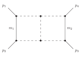
Figure 1: The H-graph. Solid lines denote massive objects, dashed lines denote massless particles.

The name H-graph stems from the fact that the gravitons form the letter “H” (which in our figure is rotated by $90^{\circ}$). In order to describe the kinematics we introduce the Mandelstam variables

$$s\;=\;\left(p_{1}+p_{2}\right)^{2}, t\;=\;\left(p_{2}+p_{3}\right)^{2}.$$ (1)

The external momenta are on-shell:

$$p_{1}^{2}\;=\;p_{2}^{2}\;=\;m_{1}^{2}, p_{3}^{2}\;=\;p_{4}^{2}\;=\;m_{2}^{2}.$$ (2)

For a binary system the limit $|s|\ll t,m_{1}^{2},m_{2}^{2}$ is relevant. Nevertheless, a calculation without approximations is helpful. We distinguish two cases:

$$\mbox{Equal mass case}: m_{1}=m_{2}=m.$$

$$\mbox{Unequal mass case}: m_{1}\neq m_{2}.$$ (3)

The equal mass case has been first studied in [37]. The first steps of our calculation are standard: We use integration-by-parts identities [38, 39] to derive the differential equation for the master integrals $I$ [40, 41, 42, 43]

$$dI = AI.$$ (4)

The differential equation can be cast to an $\varepsilon$-form [44]:

$$A = \varepsilon\sum\limits_{k=1}^{N_{\mathrm{letter}}}C_{k}\omega_{k},\;\;\;\;\;\;\omega_{k}\;=\;d\ln f_{k}.$$ (5)

In our case the $f_{k}$’s are algebraic functions of the kinematic variables, i.e. the $f_{k}$’s may contain square roots. Our system of master integrals is characterised by the number kinematic variables $N_{\mathrm{kin}}$, the number of master integrals $N_{\mathrm{master}}$, the number of distinct square roots $N_{\mathrm{root}}$ and the number of letters $N_{\mathrm{letter}}$. Table 1 summarises these numbers for the equal and unequal mass case.

Equal mass case:	Unequal mass case:
$2$ kinematic variables $s/m^{2}$, $t/m^{2}$	$3$ kinematic variables $s/m_{1}^{2}$, $t/m_{1}^{2}$, $m_{2}^{2}/m_{1}^{2}$
$25$ master integrals	$40$ master integrals
$4$ square roots	$6$ square roots
$17$ dlog-forms	$29$ dlog-forms

Table 1: The essential numbers for the equal and unequal mass case.

The differential equation (4) is solved in terms of Chen’s iterated integrals $I_{\gamma}(\omega_{i_{1}},\dots,\omega_{i_{r}})$ [45]. We are interested in the question if these iterated integrals (say up to weight four) can be converted to standard functions (i.e. multiple polylogarithms). The complication is given by the occurrence of the square roots. In the unequal mass case the occurring square roots are

$$r_{1} =\sqrt{-s\left(4m_{1}^{2}-s\right)}, r_{4} =\sqrt{-s\left[4m_{1}^{2}m_{2}^{4}-s\left(m_{1}^{2}-t\right)^{2}\right]},$$ (6)

$$r_{2} =\sqrt{-s\left(4m_{2}^{2}-s\right)}, r_{5} =\sqrt{-s\left[4m_{1}^{4}m_{2}^{2}-s\left(m_{2}^{2}-t\right)^{2}\right]},$$

$$r_{3} =\sqrt{\left[\left(m_{1}-m_{2}\right)^{2}-t\right]\left[\left(m_{1}+m_{2}\right)^{2}-t\right]}, r_{6} =\sqrt{\left[\left(m_{1}-m_{2}\right)^{2}-s-t\right]\left[\left(m_{1}+m_{2}\right)^{2}-s-t\right]}.$$

In the equal mass case $r_{1}$ and $r_{2}$ become identical, and so do $r_{4}$ and $r_{5}$.

We remark that the scalar double box integral with no dots and no irreducible scalar products has up to weight four a rather simple expression in terms of multiple polylogarithms. In the equal mass case we have

$$\frac{1}{\varepsilon^{4}s^{2}r_{3}}I_{1111111} = 4\left[G\left(1,1,1;\bar{y}\right)+\zeta_{2}G\left(1;\bar{y}\right)\right]\varepsilon^{3}+4\left\{2G\left(2,1,1,1;\bar{y}\right)\right.$$ (7)

$$\left.+2G\left(0,1,1,1;\bar{y}\right)-2G\left(1,1,2,1;\bar{y}\right)-2G\left(1,1,0,1;\bar{y}\right)\right.$$

$$\left.+2\zeta_{2}\left[G\left(2,1;\bar{y}\right)+G\left(0,1;\bar{y}\right)-G\left(1,1;\bar{y}\right)\right]-\zeta_{3}G\left(1;\bar{y}\right)\right.$$

$$\left.+2\left[G\left(1,1,1;\bar{y}\right)+\zeta_{2}G\left(1;\bar{y}\right)\right]\left[G\left(1,\bar{x}\right)-2\ln\left(\bar{x}\right)\right]\right\}\varepsilon^{4}+{\mathcal{O}}\left(\varepsilon^{5}\right),$$

$$s\;=\;-\frac{\bar{x}^{2}}{1-\bar{x}}m^{2},\;\;\;\;\;\;t\;=\;-\frac{\bar{y}^{2}}{1-\bar{y}}m^{2}.$$

and similar for the unequal mass case. We are interested in all master integrals up to weight four. The remaining master integrals in the top sector as well as master integrals from sub-sectors will involve non-trivial subsets of the square roots up to weight $4$. The most challenging topologies are shown in fig. 2.

unequal:	4 masters	5 masters	3 masters
equal:	3 masters	4 masters	3 masters

Figure 2: Topologies with a dependence up to weight $4$ on a non-trivial subset of the square roots.

2 Rationalisation of square roots

By a change of variables it is sometimes possible to rationalise a square root. Let us look at a simple example. Consider a dlog-form with a square root:

$$\omega = d\ln\left(\frac{2m_{1}^{2}-s-r_{1}}{2m_{1}^{2}-s+r_{1}}\right)\;=\;\frac{2s}{r_{1}}\left(\frac{ds}{s}-\frac{dm_{1}^{2}}{m_{1}^{2}}\right)$$ (8)

The transformation

$$-\frac{s}{m_{1}^{2}} = \frac{\left(1-x\right)^{2}}{x}$$ (9)

rationalises the square root:

$$\omega = 2d\ln\left(x\right)\;=\;2\frac{dx}{x}$$ (10)

Let us assume that the differential equation is in $\varepsilon$-dlog-form, where the arguments of the logarithms contain square roots. There are algorithms to rationalise square roots [46, 47]. If we can simultaneously rationalise all square roots, all integrals can be expressed in terms of multiple polylogarithms. It can be hard to prove that the set of square roots cannot be rationalised simultaneously [48]. Even if one can prove that a set of square roots cannot be rationalised simultaneously, this does not imply that the Feynman integrals cannot be expressed in terms of multiple polylogarithms [49]. Hence, being able to rationalise simultaneously all square roots is a sufficient condition that the result can be expressed in terms of multiple polylogarithms, but not a necessary condition. If a set of square roots cannot be rationalised simultaneously, other methods like symbol calculus [49, 50] or introducing additional variables [51, 52, 53, 54] may express the Feynman integrals in terms of multiple polylogarithms.

Multiple square roots appear not only in the Feynman integrals associated to the H-graph, but also in Feynman integrals associated to other processes. Example are Bhabha scattering [55] or Drell-Yan [56]. As we study more two-loop integrals with several kinematic variables, multiple square roots become more frequent. We want to learn how to handle them.

We therefore study the case of the H-graph in more detail. We first note that the last square root $r_{6}$ appears up to weight $4$ only in one master integral (one master integral from the sub-topology shown in the middle in fig. 2). This master integral can be computed in the Feynman parameter representation and evaluates to multiple polylogarithms following the lines of [57, 58, 49]. This holds in the equal mass case and in the unequal mass case.

In the equal mass case we then have the following situation: The remaining 24 master integrals involve up to weight $4$ only three square roots. These square roots can be rationalised simultaneously and therefore all master integrals evaluate up to weight $4$ to multiple polylogarithms [59].

The unequal mass case is more complicated: Each master integral is a linear combination of iterated integrals. Each iterated integral of the master integrals contains up to weight $4$ no more than $3$ distinct roots. In the remaining 39 master integrals up to weight $4$ each occurring triple of distinct roots can be rationalised simultaneously. In other words: we can rationalise simultaneously any occurring triple $(r_{i},r_{j},r_{k})$ from $\{r_{1},r_{2},r_{3},r_{4},r_{5}\}$, but we may have to use different rationalisations for different triples. This raises the question whether we are allowed to use different rationalisations for different iterated integrals. We have to distinguish two cases:

1. Different rationalisations may correspond to different parametrisations of the same integration path (left picture of fig. 3).

2. Different rationalisations may correspond to different integration paths (right picture of fig. 3).

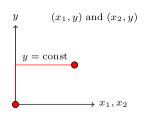
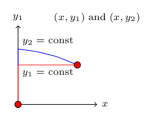
Figure 3: The left picture shows two parametrisations of the same integration path, the right picture shows two different integration paths.

Case $1$ is unproblematic and we therefore discuss case $2$. A single iterated integral $I_{\gamma}(\omega_{1},\dots,\omega_{r})$ is in general path dependent. The linear combination of iterated integrals in the $\varepsilon^{j}$-term of the $i$-th master integral $I_{i}^{(j)}$ is path independent, this is ensured by the integrability condition of the differential equation $dA-A\wedge A=0$. This allows us to use different integration paths for $I_{i_{1}}^{(j_{1})}$ and $I_{i_{2}}^{(j_{2})}$.

Now let’s look at a single expression $I_{i}^{(j)}$: We would like to split

$$I_{i}^{(j)} = I_{i,a}^{(j)}+I_{i,b}^{(j)}$$ (11)

and use different integration paths for $I_{i,a}^{(j)}$ and $I_{i,b}^{(j)}$. This is only allowed if $I_{i,a}^{(j)}$ and $I_{i,b}^{(j)}$ are path independent. In order to give a criteria when a linear combination of iterated integrals is path independent we first introduce the bar notation for the tensor algebra (we assume that all $\omega_{j}$’s are closed):

$$\left[\omega_{1}|\omega_{2}|\dots|\omega_{r}\right] = \omega_{1}\otimes\omega_{2}\otimes\dots\otimes\omega_{r},$$

$$d\left[\omega_{1}|\omega_{2}|\dots|\omega_{r}\right] = \sum\limits_{j=1}^{r-1}\left[\omega_{1}|\dots|\omega_{j-1}|\omega_{j}\wedge\omega_{j+1}|\omega_{j+2}|\dots|\omega_{r}\right].$$ (12)

We associate to a linear combination of iterated integrals

$$I\;=\;\sum\limits_{j=1}^{r}\sum\limits_{i_{1},\dots,i_{j}}c_{i_{1}\dots i_{j}}I_{\gamma}\left(\omega_{i_{1}},\dots,\omega_{i_{j}}\right) \Rightarrow B\;=\;\sum\limits_{j=1}^{r}\sum\limits_{i_{1},\dots,i_{j}}c_{i_{1}\dots i_{j}}\left[\omega_{i_{1}}|\dots|\omega_{i_{j}}\right]$$ (13)

By a theorem of Chen [45] the linear combination $I$ is path independent if and only if $dB=0$.

For the case at hand, we observe that $\omega_{i}\wedge\omega_{j}$ may involve less square roots than $\omega_{i}\otimes\omega_{j}$. Although $I_{i,a}^{(j)}$ and $I_{i,b}^{(j)}$ may be path dependent, we may find $I_{\mathrm{subtr}}^{(j)}$ compatible with two rationalisations such that

$$\left(I_{i,a}^{(j)}-I_{\mathrm{subtr}}^{(j)}\right) \left(I_{i,b}^{(j)}+I_{\mathrm{subtr}}^{(j)}\right)$$ and (14)

are path independent. We may then evaluate $(I_{i,a}^{(j)}-I_{\mathrm{subtr}}^{(j)})$ with a rationalisation corresponding to an integration path $\gamma_{a}$ and $(I_{i,b}^{(j)}+I_{\mathrm{subtr}}^{(j)})$ with a rationalisation corresponding to an integration path $\gamma_{b}$. The subtraction terms can be obtained from Stokes’ theorem by integrating $\omega_{i}\wedge\omega_{j}$, as sketched in fig. 4.

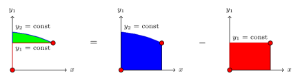
Figure 4: The difference of two integration paths defines an area (green), which we write may write as the difference of two areas, where each area only knows about one integration path.

We remark that in mathematical terms, $I_{\mathrm{subtr}}^{(j)}$ is related to Massey products.

Let us discuss another pitfall, which may occur when using different rationalisations. This pitfall may occur already for different parametrisations of the same integration path and is related to trailing zeros. Consider the transformation $x=2x^{\prime}$ and the dlog-form

$$\omega_{0}\;=\;d\ln(x)\;=\;d\ln(2x^{\prime})\;=\;d\left[\ln(2)+\ln(x^{\prime})\right]\;=\;d\ln(x^{\prime}).$$ (15)

Consider the apparent contradiction

$$\int\limits_{0}^{x_{f}}\omega_{0}\;=\;\ln(x_{f}) \neq \ln(x_{f})-ln(2)\;=\;\ln(x_{f}^{\prime})\;=\;\int\limits_{0}^{x_{f}^{\prime}}\omega_{0}.$$ (16)

The solution to this contradiction is as follows: The two integrals appearing in eq. (16) are divergent integrals. Although it is common practice to define

$$\int\limits_{0}^{x_{f}}\frac{dx}{x} = \ln(x_{f}),$$ (17)

we should not forget what this notation actually means: We first introduce a lower cut-off $\lambda$ as a regulator. In a second step we employ a “renormalisation scheme” and remove all $\ln(\lambda)$-terms. It is now clear what the solution has to be: A transformation $x=2x^{\prime}$ induces a change of the “renormalisation scheme”. In practice this boils down to that we isolate all trailing zeros in $x^{\prime}$ and substitute

$$\ln(x^{\prime}) \rightarrow \ln(x^{\prime})+\ln(2).$$ (18)

3 Conclusion

In this talk we discussed the computation of the master integrals of the two-loop H-graph, relevant to gravitational waves. The differential equation for the master integrals involves four square roots in the equal mass case and six square roots in the unequal mass case. The major challenge is a method for an efficient computation for the case where not all square roots can be rationalised simultaneously. In the equal mass case we found that all master integrals up to weight 4 can be expressed in terms of multiple polylogarithms. For the unequal mass case we reported on techniques to render sub-expressions of iterated integrals path-independent.

References

- [1] A. Buonanno and T. Damour, Effective one-body approach to general relativistic two-body dynamics, Phys. Rev. D 59, 084006 (1999), 10.1103/PhysRevD.59.084006, gr-qc/9811091.
- [2] A. Buonanno and T. Damour, Transition from inspiral to plunge in binary black hole coalescences, Phys. Rev. D 62, 064015 (2000), 10.1103/PhysRevD.62.064015, gr-qc/0001013.
- [3] T. Damour, The General Relativistic Two Body Problem and the Effective One Body Formalism, Fundam. Theor. Phys. 177, 111 (2014), 10.1007/978-3-319-06349-2_5, 1212.3169.
- [4] T. Damour and P. Jaranowski, Four-loop static contribution to the gravitational interaction potential of two point masses, Phys. Rev. D 95(8), 084005 (2017), 10.1103/PhysRevD.95.084005, 1701.02645.
- [5] D. Bini, T. Damour and A. Geralico, Sixth post-Newtonian local-in-time dynamics of binary systems, Phys. Rev. D 102(2), 024061 (2020), 10.1103/PhysRevD.102.024061, 2004.05407.
- [6] D. Bini, T. Damour and A. Geralico, Sixth post-Newtonian nonlocal-in-time dynamics of binary systems, Phys. Rev. D 102(8), 084047 (2020), 10.1103/PhysRevD.102.084047, 2007.11239.
- [7] W. D. Goldberger and I. Z. Rothstein, An Effective field theory of gravity for extended objects, Phys. Rev. D 73, 104029 (2006), 10.1103/PhysRevD.73.104029, hep-th/0409156.
- [8] C. Cheung, I. Z. Rothstein and M. P. Solon, From Scattering Amplitudes to Classical Potentials in the Post-Minkowskian Expansion, Phys. Rev. Lett. 121(25), 251101 (2018), 10.1103/PhysRevLett.121.251101, 1808.02489.
- [9] R. A. Porto, The effective field theorist’s approach to gravitational dynamics, Phys. Rept. 633, 1 (2016), 10.1016/j.physrep.2016.04.003, 1601.04914.
- [10] M. Levi, Effective Field Theories of Post-Newtonian Gravity: A comprehensive review, Rept. Prog. Phys. 83(7), 075901 (2020), 10.1088/1361-6633/ab12bc, 1807.01699.
- [11] S. Foffa, P. Mastrolia, R. Sturani and C. Sturm, Effective field theory approach to the gravitational two-body dynamics, at fourth post-Newtonian order and quintic in the Newton constant, Phys. Rev. D 95(10), 104009 (2017), 10.1103/PhysRevD.95.104009, 1612.00482.
- [12] S. Foffa, P. Mastrolia, R. Sturani, C. Sturm and W. J. Torres Bobadilla, Static two-body potential at fifth post-Newtonian order, Phys. Rev. Lett. 122(24), 241605 (2019), 10.1103/PhysRevLett.122.241605, 1902.10571.
- [13] D. Bini, T. Damour, A. Geralico, S. Laporta and P. Mastrolia, Gravitational dynamics at : perturbative gravitational scattering meets experimental mathematics (2020), 2008.09389.
- [14] D. Bini, T. Damour, A. Geralico, S. Laporta and P. Mastrolia, Gravitational scattering at the seventh order in : nonlocal contribution at the sixth post-Newtonian accuracy, Phys. Rev. D 103(4), 044038 (2021), 10.1103/PhysRevD.103.044038, 2012.12918.
- [15] N. E. J. Bjerrum-Bohr, P. H. Damgaard, G. Festuccia, L. Planté and P. Vanhove, General Relativity from Scattering Amplitudes, Phys. Rev. Lett. 121(17), 171601 (2018), 10.1103/PhysRevLett.121.171601, 1806.04920.
- [16] A. Cristofoli, N. E. J. Bjerrum-Bohr, P. H. Damgaard and P. Vanhove, Post-Minkowskian Hamiltonians in general relativity, Phys. Rev. D 100(8), 084040 (2019), 10.1103/PhysRevD.100.084040, 1906.01579.
- [17] D. A. Kosower, B. Maybee and D. O’Connell, Amplitudes, Observables, and Classical Scattering, JHEP 02, 137 (2019), 10.1007/JHEP02(2019)137, 1811.10950.
- [18] Z. Bern, C. Cheung, R. Roiban, C.-H. Shen, M. P. Solon and M. Zeng, Scattering Amplitudes and the Conservative Hamiltonian for Binary Systems at Third Post-Minkowskian Order, Phys. Rev. Lett. 122(20), 201603 (2019), 10.1103/PhysRevLett.122.201603, 1901.04424.
- [19] Z. Bern, C. Cheung, R. Roiban, C.-H. Shen, M. P. Solon and M. Zeng, Black Hole Binary Dynamics from the Double Copy and Effective Theory, JHEP 10, 206 (2019), 10.1007/JHEP10(2019)206, 1908.01493.
- [20] Z. Bern, J. Parra-Martinez, R. Roiban, M. S. Ruf, C.-H. Shen, M. P. Solon and M. Zeng, Scattering Amplitudes and Conservative Binary Dynamics at , Phys. Rev. Lett. 126(17), 171601 (2021), 10.1103/PhysRevLett.126.171601, 2101.07254.
- [21] J. Blümlein, A. Maier and P. Marquard, Five-Loop Static Contribution to the Gravitational Interaction Potential of Two Point Masses, Phys. Lett. B 800, 135100 (2020), 10.1016/j.physletb.2019.135100, 1902.11180.
- [22] J. Blümlein, A. Maier, P. Marquard, G. Schäfer and C. Schneider, From Momentum Expansions to Post-Minkowskian Hamiltonians by Computer Algebra Algorithms, Phys. Lett. B 801, 135157 (2020), 10.1016/j.physletb.2019.135157, 1911.04411.
- [23] J. Blümlein, A. Maier, P. Marquard and G. Schäfer, Fourth post-Newtonian Hamiltonian dynamics of two-body systems from an effective field theory approach, Nucl. Phys. B 955, 115041 (2020), 10.1016/j.nuclphysb.2020.115041, 2003.01692.
- [24] J. Blümlein, A. Maier, P. Marquard and G. Schäfer, Testing binary dynamics in gravity at the sixth post-Newtonian level, Phys. Lett. B 807, 135496 (2020), 10.1016/j.physletb.2020.135496, 2003.07145.
- [25] J. Blümlein, A. Maier, P. Marquard and G. Schäfer, The fifth-order post-Newtonian Hamiltonian dynamics of two-body systems from an effective field theory approach: potential contributions, Nucl. Phys. B 965, 115352 (2021), 10.1016/j.nuclphysb.2021.115352, 2010.13672.
- [26] J. Blümlein, A. Maier, P. Marquard and G. Schäfer, The 6th post-Newtonian potential terms at , Phys. Lett. B 816, 136260 (2021), 10.1016/j.physletb.2021.136260, 2101.08630.
- [27] S. Foffa and R. Sturani, Conservative dynamics of binary systems to fourth Post-Newtonian order in the EFT approach I: Regularized Lagrangian, Phys. Rev. D 100(2), 024047 (2019), 10.1103/PhysRevD.100.024047, 1903.05113.
- [28] S. Foffa, R. A. Porto, I. Rothstein and R. Sturani, Conservative dynamics of binary systems to fourth Post-Newtonian order in the EFT approach II: Renormalized Lagrangian, Phys. Rev. D 100(2), 024048 (2019), 10.1103/PhysRevD.100.024048, 1903.05118.
- [29] G. Kälin and R. A. Porto, From Boundary Data to Bound States, JHEP 01, 072 (2020), 10.1007/JHEP01(2020)072, 1910.03008.
- [30] G. Kälin and R. A. Porto, From boundary data to bound states. Part II. Scattering angle to dynamical invariants (with twist), JHEP 02, 120 (2020), 10.1007/JHEP02(2020)120, 1911.09130.
- [31] G. Kälin and R. A. Porto, Post-Minkowskian Effective Field Theory for Conservative Binary Dynamics, JHEP 11, 106 (2020), 10.1007/JHEP11(2020)106, 2006.01184.
- [32] G. Kälin, Z. Liu and R. A. Porto, Conservative Dynamics of Binary Systems to Third Post-Minkowskian Order from the Effective Field Theory Approach, Phys. Rev. Lett. 125(26), 261103 (2020), 10.1103/PhysRevLett.125.261103, 2007.04977.
- [33] Z. Liu, R. A. Porto and Z. Yang, Spin Effects in the Effective Field Theory Approach to Post-Minkowskian Conservative Dynamics, JHEP 06, 012 (2021), 10.1007/JHEP06(2021)012, 2102.10059.
- [34] E. Herrmann, J. Parra-Martinez, M. S. Ruf and M. Zeng, Gravitational Bremsstrahlung from Reverse Unitarity, Phys. Rev. Lett. 126(20), 201602 (2021), 10.1103/PhysRevLett.126.201602, 2101.07255.
- [35] P. Di Vecchia, C. Heissenberg, R. Russo and G. Veneziano, The eikonal approach to gravitational scattering and radiation at (G3), JHEP 07, 169 (2021), 10.1007/JHEP07(2021)169, 2104.03256.
- [36] N. E. J. Bjerrum-Bohr, P. H. Damgaard, L. Planté and P. Vanhove, Classical gravity from loop amplitudes, Phys. Rev. D 104(2), 026009 (2021), 10.1103/PhysRevD.104.026009, 2104.04510.
- [37] M. S. Bianchi and M. Leoni, A planar double box in canonical form, Phys. Lett. B777, 394 (2018), 10.1016/j.physletb.2017.12.030, 1612.05609.
- [38] F. V. Tkachov, A theorem on analytical calculability of four loop renormalization group functions, Phys. Lett. B100, 65 (1981).
- [39] K. G. Chetyrkin and F. V. Tkachov, Integration by parts: The algorithm to calculate beta functions in 4 loops, Nucl. Phys. B192, 159 (1981).
- [40] A. V. Kotikov, Differential equations method: New technique for massive feynman diagrams calculation, Phys. Lett. B254, 158 (1991).
- [41] A. V. Kotikov, Differential equation method: The calculation of n point feynman diagrams, Phys. Lett. B267, 123 (1991).
- [42] E. Remiddi, Differential equations for feynman graph amplitudes, Nuovo Cim. A110, 1435 (1997), hep-th/9711188.
- [43] T. Gehrmann and E. Remiddi, Differential equations for two-loop four-point functions, Nucl. Phys. B580, 485 (2000), hep-ph/9912329.
- [44] J. M. Henn, Multiloop integrals in dimensional regularization made simple, Phys. Rev. Lett. 110, 251601 (2013), 10.1103/PhysRevLett.110.251601, 1304.1806.
- [45] K.-T. Chen, Iterated path integrals, Bull. Amer. Math. Soc. 83, 831 (1977).
- [46] M. Besier, D. Van Straten and S. Weinzierl, Rationalizing roots: an algorithmic approach, Commun. Num. Theor. Phys. 13, 253 (2019), 10.4310/CNTP.2019.v13.n2.a1, 1809.10983.
- [47] M. Besier, P. Wasser and S. Weinzierl, RationalizeRoots: Software Package for the Rationalization of Square Roots, Comput. Phys. Commun. 253, 107197 (2020), 10.1016/j.cpc.2020.107197, 1910.13251.
- [48] M. Besier, D. Festi, M. Harrison and B. Naskręcki, Arithmetic and geometry of a K3 surface emerging from virtual corrections to Drell–Yan scattering, Commun. Num. Theor. Phys. 14(4), 863 (2020), 10.4310/CNTP.2020.v14.n4.a4, 1908.01079.
- [49] M. Heller, A. von Manteuffel and R. M. Schabinger, Multiple polylogarithms with algebraic arguments and the two-loop EW-QCD Drell-Yan master integrals, Phys. Rev. D 102(1), 016025 (2020), 10.1103/PhysRevD.102.016025, 1907.00491.
- [50] M. Heller, Planar two-loop integrals for scattering in QED with finite lepton masses (2021), 2105.08046.
- [51] C. G. Papadopoulos, Simplified differential equations approach for Master Integrals, JHEP 07, 088 (2014), 10.1007/JHEP07(2014)088, 1401.6057.
- [52] C. G. Papadopoulos, D. Tommasini and C. Wever, Two-loop Master Integrals with the Simplified Differential Equations approach, JHEP 01, 072 (2015), 10.1007/JHEP01(2015)072, 1409.6114.
- [53] C. G. Papadopoulos, D. Tommasini and C. Wever, The Pentabox Master Integrals with the Simplified Differential Equations approach, JHEP 04, 078 (2016), 10.1007/JHEP04(2016)078, 1511.09404.
- [54] D. D. Canko, C. G. Papadopoulos and N. Syrrakos, Analytic representation of all planar two-loop five-point Master Integrals with one off-shell leg, JHEP 01, 199 (2021), 10.1007/JHEP01(2021)199, 2009.13917.
- [55] J. M. Henn and V. A. Smirnov, Analytic results for two-loop master integrals for Bhabha scattering I, JHEP 11, 041 (2013), 10.1007/JHEP11(2013)041, 1307.4083.
- [56] R. Bonciani, S. Di Vita, P. Mastrolia and U. Schubert, Two-Loop Master Integrals for the mixed EW-QCD virtual corrections to Drell-Yan scattering, JHEP 09, 091 (2016), 10.1007/JHEP09(2016)091, 1604.08581.
- [57] F. Brown, The massless higher-loop two-point function, Commun. Math. Phys. 287, 925 (2008), 0804.1660.
- [58] E. Panzer, Algorithms for the symbolic integration of hyperlogarithms with applications to Feynman integrals, Comput. Phys. Commun. 188, 148 (2014), 10.1016/j.cpc.2014.10.019, 1403.3385.
- [59] P. A. Kreer and S. Weinzierl, The H-graph with equal masses in terms of multiple polylogarithms, Phys. Lett. B 819, 136405 (2021), 10.1016/j.physletb.2021.136405, 2104.07488.