Black Hole Binary Dynamics from the Double Copy and Effective Theory

Abstract

We describe a systematic framework for computing the conservative potential of a compact binary system using modern tools from scattering amplitudes and effective field theory. Our approach combines methods for integration and matching adapted from effective field theory, generalized unitarity, and the double-copy construction, which relates gravity integrands to simpler gauge-theory expressions. With these methods we derive the third post-Minkowskian correction to the conservative two-body Hamiltonian for spinless black holes. We describe in some detail various checks of our integration methods and the resulting Hamiltonian.

1 Introduction

The extraordinary detection of gravitational waves by the LIGO and Virgo collaborations 1602.03837 ; 1710.05832 has opened a new window into the cosmos. Gravitational wave astronomy is now a critical tool for answering longstanding questions in astronomy and cosmology, and offers a test of gravity in violent environments never before probed by experiment.

The LIGO and Virgo detectors boast an exquisite precision which will grow in future upgrades, thus demanding commensurately accurate theoretical predictions encoded in waveform templates utilized for detection and extraction of source parameters. These waveforms are constructed from an array of complementary approaches, including the effective one-body (EOB) formalism gr-qc/9811091 ; gr-qc/0001013 , numerical relativity gr-qc/0507014 ; gr-qc/0511048 ; gr-qc/0511103 , the self-force formalism gr-qc/9606018 ; gr-qc/9610053 , and a number of perturbative methods for the inspiral phase, including the post-Newtonian (PN) Droste ; EIH and post-Minkowskian (PM) PM1 ; PM2 ; PM3 ; PM4 ; PM5 ; PM6 ; PM7 ; PM8 ; Westpfahl2PM ; Damour:2016gwp ; DamourTwoLoop approximations, as well as the nonrelativistic general relativity (NRGR) formalism NRGR based on effective field theory (EFT). For recent reviews see Refs. 1310.1528 ; 1601.04914 ; 1805.07240 ; 1805.10385 ; 1806.05195 ; 1807.01699 and references therein. In the coming years, further improvements in high-precision theoretical predictions from general relativity will be essential given expected improvements in detector sensitivity.

During the early inspiral phase, the gravitational field is weak and the constituents of binary black hole system are non-relativistic. In the PN approximation, we organize the interaction Hamiltonian as an expansion in

$$\bm{v}^{2}\sim\frac{Gm}{|\bm{r}|}\ll 1\,,$$ (1.1)

where $G$ is Newton’s constant and $m$ is the total mass of the binary system, while $\bm{v}$ and $\bm{r}$ are the relative velocity and position between the black holes in units with $c=1$. The PN expansion is a double expansion in the velocity squared and the inverse separation in units of the Schwarzschild radius, which are of order each other due to the virial theorem. The powers in $G$ and $\bm{v}$ corresponding to each PN order are depicted in Fig. 1.

In the present work we focus on conservative dynamics. The PN perturbative framework is well-established with a long history dating back to the leading 1PN correction to the Newtonian gravitational potential, which was computed by Einstein, Infeld, and Hoffman EIH . Later pioneering work derived the full 2PN 2PNOhta , 3PN Jaranowski:1997ky ; gr-qc/9912092 ; gr-qc/0004009 ; gr-qc/0105038 , and 4PN JaranowskSchafer1 ; JaranowskSchafer2 ; Bernard:2015njp ; Marchand:2017pir ; Foffa:2012rn ; Foffa:2016rgu ; Foffa:2019rdf ; arXiv:1703.06433 ; arXiv:1903.05118 expressions for the conservative potential. More recently, 5PN static contributions have also been computed 1902.10571 ; 1902.11180 .

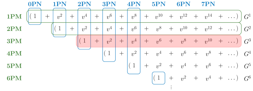
Figure 1: A summary of known results for the two-body potential for spinless black holes in the PN and PM expansions, outlined in blue and green regions respectively. The new 3PM result summarized in LABEL:3PMPRL and discussed at length in this paper is highlighted in the shaded (red) region. The overlap gives strong crosschecks on any calculations in either approach.

In contrast, the PM expansion is organized differently, including instead contributions to all orders in velocity at fixed order in $G$. So when we refer to the $n$PM correction, we refer to a contribution which, when expanded in $\bm{v}$, generates all PN terms at order $G^{n}$. In particular, when expanded to ${\bm{v}}^{6}$ order, the 3PM result gives a previously unknown contribution to the 5PN potential. The powers in $G$ and $\bm{v}$ corresponding to each PM order are shown Fig. 1. This expansion has recently received new attention Damour:2016gwp ; 1805.00813 ; 1806.08347 ; CachazoGuevara ; 1709.00590 ; 1709.06016 ; 1805.10809 ; 1812.06895 ; 1812.00956 ; 1812.08752 ; 1906.09260 ; 1906.10071 ; Plefka ; CliffIraMikhailClassical ; 3PMPRL ; Paolo2PM ; Cristofoli:2019neg ; 1905.05657 ; 1906.05209 , based in part on the connection of classical physics to quantum scattering amplitudes Iwasaki:1971vb ; Iwasaki:1971iy ; Gupta:1979br ; gr-qc/9405057 ; hep-th/0405239 ; RothsteinClassical ; Vaidya:2014kza ; OConnellObservables . Relativistic scattering amplitudes are naturally organized as a series in powers of the coupling $G$, keeping all orders in the velocity, and for this purpose we define the PM potential to be

$$V(\bm{p},\bm{r}) =\sum_{n=1}^{\infty}\left(\frac{G}{|\bm{r}|}\right)^{n}c_{n}(\bm{p}^{2})\,,$$ (1.2)

where the coefficients $c_{n}$ are functions of $\bm{p}\sim\bm{v}$ which contain arbitrarily high powers in the velocity. Of course, whether the new information in PM dynamics can be directly used to improve gravitational wave templates for inspiraling binary systems requires detailed study, e.g. along the lines of Ref. Antonelli:2019ytb . Nonetheless, at the very least, as can be seen from Fig. 1 the PM approximation is complementary to the PN approximation, providing results for a subset of terms at each PN order.

The primary goal of this paper is to develop efficient methods for high-precision predictions of the dynamics of gravitationally bound compact objects. By using scattering amplitudes as the starting point, we take advantage of the enormous progress in the past decade for computing and understanding them in gravitational theories, with systematically improvable precision. This includes applying generalized unitarity hep-ph/9403226 ; hep-ph/9409265 ; hep-ph/9708239 ; hep-th/0412103 ; 0705.1864 ; hep-ph/9602280 ; 1103.1869 ; 1103.3298 and double-copy constructions KLT ; BCJ ; BCJLoop , which have enabled explicit (super)gravity calculations at remarkably high orders of perturbation theory SimplifyingBCJ ; 0905.2326 ; SimplifyingBCJ ; 1309.2498 ; 1409.3089 ; 1708.06807 ; 1804.09311 ; 1507.06118 ; 1701.02422 . The double copy allows us to express gravitational scattering amplitudes in terms of corresponding simpler gauge theory amplitudes, while generalized unitarity gives a means for building loop amplitudes from simpler tree amplitudes. As we shall see, these can also be combined with spinor-helicity methods Berends:1981rb ; Berends:1981uq ; Xu:1986xb which then yield amazingly compact expressions for unitarity cuts that contain all information required to build the classical potential at 3PM.

The central idea in relating scattering amplitudes to the orbital dynamics of compact binaries is that both processes are governed by the same underlying theory. By construction, the effective two-body potential in Eq. (1.2) reproduces the same physics as the full gravitational theory for kinematics defined by massive bodies interacting via a classical long-range force. We can therefore extract the effective potential from scattering amplitudes, which are convenient to calculate using modern field theory tools. This was demonstrated long ago Iwasaki:1971vb ; Iwasaki:1971iy ; Gupta:1979br ; gr-qc/9405057 ; hep-th/0405239 , and recently revived using EOB DamourTwoLoop and EFT RothsteinClassical ; Vaidya:2014kza methods, including those that incorporate corrections to all orders in velocity. The EFT approach has led to new results for the PM potential at higher orders CliffIraMikhailClassical ; 3PMPRL . As we shall see, EFT methods are not only useful for systematically mapping scattering amplitudes to classical potentials but also for efficiently dealing with the integrals encountered in the full theory CliffIraMikhailClassical .

The combination of these key ingredients from the modern amplitudes program and effective field theory led to a remarkably compact expression for the classical 3PM conservative two-body potential 3PMPRL . This result is state of the art. As shown in Fig. 1, it provides new information not obtained previously by PN or effective one-body methods, and a strong independent crosscheck of known terms in the PN expansion. Furthermore, these results have already been examined by LIGO theorists Antonelli:2019ytb and compared against lower order PM calculations, numerical relativity, and various effective one-body models.

The present paper is a companion to the Letter 3PMPRL summarizing our results for the 3PM conservative Hamiltonian. Our aim is to fill in the various technical details, and the analysis will be divided into several parts. First, we introduce the basic tools for extracting classical potentials from quantum scattering amplitudes. Quantum gravitational amplitudes encode in principle the physics of both bound quasi-elliptic orbits and unbound quasi-hyperbolic orbits in a relativistic manner that is well suited for the PM expansion. They are however quite complicated, and important simplifications arise by truncating away quantum contributions as early as possible in the calculation. In Sec. 2, we discuss the kinematics, hierarchies of scales, and power counting that allow us to identify a precise demarcation between classical and quantum contributions to the scattering amplitude at the integrand level. The latter distinction is crucial for the scalability of the method to higher-loop orders since integration of full quantum integrands prior to classical expansion is not viable with current technology.

Second, we use the double copy and generalized unitarity to obtain the relativistic integrands relevant for one- and two-loop classical scattering of massive gravitationally interacting scalars. As discussed in Sec. 3, the starting point of our construction are remarkably compact four- and five-point gauge-theory tree-level scattering amplitudes. Using double-copy methods, these are converted to appropriate tree-level gravitational scattering amplitudes, which are then combined into generalized unitarity cuts in order to build loop integrands. By identifying terms that cannot contribute to the classical potential, we are able to vastly reduce the complexity of these expressions. Details of the construction using various helicity and double-copy methods as well as explicit results at one and two loops are given in Sec. 4, Sec. 5, and Sec. 6.

Third, to obtain the parts of the scattering amplitudes needed for building the classical potential, we integrate the relativistic integrands via an assortment of old and newly developed tools. We consider both nonrelativistic and relativistic methods of integration, which are discussed in Sec. 7 and Sec. 8, respectively. The former approach is an adaptation of the method of regions Beneke:1997zp ; Smirnov:2004ym and mimics the mechanics of NRGR NRGR in that integration occurs via a reduction to three-dimensional bubble integrals. While this method obscures relativistic covariance, it is very efficient and by design scalable to high loop order. The latter approach includes the methods of differential equations and Mellin-Barnes integration which produce exact results to all orders in velocity for certain diagram topologies. In Sec. 9 we give the integrated answers for the contributing diagrams, discuss the resummation of the results from nonrelativistic integration, and present the final amplitude containing all contributions to the 3PM potential in Eq. (9.3)

Fourth, in Sec. 10 we use effective field theory to extract the classical conservative potential from the resulting scattering amplitude. This procedure systematically implements the subtraction of infrared divergent iterated contributions in the amplitude, leaving behind the desired new contribution to the potential. The 3PM coefficients for the classical potential (1.2) are given in Eq. (10.10). A convenient byproduct of the matching is that we can choose a frame in which the potential is in a much more compact form compared to previous expressions.

Lastly, in Sec. 11 we validate our result through various checks against the existing literature. In the probe limit, our result reduces to the known potential from the Schwarzschild solution. As shown in Fig. 1, our 3PM Hamiltonian overlaps with the known 4PN result JaranowskSchafer2 , and we confirm their physical equivalence by providing the canonical transformation that maps the result of Ref. JaranowskSchafer2 to ours. We also compare results for scattering amplitudes and scattering angles computed from classical potentials. In Sec. 12, we discuss various features and subtleties. This includes the appearance of a mass singularity in the 3PM two-body potential, that four-dimensional constructions of the integrands are sufficient through 3PM order despite using dimensional regularization, and the lack of contributions from radiation modes to the conservative potential through 3PM order.

We conclude in Sec. 13, and provide several appendices. In Appendix A, we collect notation used in the paper. In Appendix B we provide the gauge-theory amplitudes that are necessary for constructing the gravitational amplitudes. In Appendix C, we collect the series that appear in our nonrelativistic integration and their resummation. In Appendix D we extract the classical limit of a two-loop Feynman integral by starting from the fully integrated result in Ref. Bianchi:2016yiq , and then take the limit in the final expression. This evaluation matches the results obtained with our methods, confirming the presence of the mass singularity. It also displays an imaginary part, connected to the presence of on-shell radiation, which does not contribute to the 3PM conservative potential.

2 Classical Versus Quantum

The goal of this section is to introduce the basic ideas for efficiently identifying the parts of quantum scattering amplitudes that contribute to the classical potential. We discuss the kinematics, scale hierarchies, power counting, and truncation of graph structures that allow us to drop quantum contributions at the integrand level. This leads to enormous simplifications that are crucial for the scalability to high loop orders.

2.1 External Matter Kinematics

Gravitationally interacting spinless compact bodies with masses $m_{1}$ and $m_{2}$ can be described by a system of two real scalar fields $\phi_{1}$ and $\phi_{2}$ minimally coupled to gravity:

$$S_{\textrm{GR}}=\int d^{D}x\sqrt{-g}\left[-\frac{1}{16\pi G}R+\frac{1}{2}\sum_{i=1,2}\left(D^{\mu}\phi_{i}D_{\mu}\phi_{i}-m_{i}^{2}\phi^{2}_{i}\right)\right]\,,$$ (2.1)

where the first term is the usual Einstein-Hilbert action. Here we consider the point-particle approximation, although finite size corrections can be systematically included using higher-dimension operators Damour:1998jk ; NRGR . Moreover, we exclude local interactions between matter fields, which violate the classical assumption that the inter-particle separation is larger than their de Broglie wavelength.

The main focus of our analysis is the elastic-scattering amplitude of $\phi_{1}$ and $\phi_{2}$ in the center of mass frame, where the incoming states have four-momenta $(E_{1},\bm{p})$ and $(E_{2},-\bm{p})$ while the outgoing states have four-momenta $(E_{1},\bm{p}^{\prime})$ and $(E_{2},-\bm{p}^{\prime})$. The energies are defined in the usual way, e.g. $E_{1}=\sqrt{\bm{p}^{2}+m_{1}^{2}}$, and the conservation of energy for each matter field implies $\bm{p}^{2}=\bm{p}^{\prime 2}$. We define the four-momentum transfer in the scattering process as

$$q=(0,\bm{q})=(0,\bm{p}-\bm{p}^{\prime})\,.$$ (2.2)

Classical physics applies whenever the minimal inter-particle separation is larger than the de Broglie wavelength, $\lambda$, of each particle. For a scattering process we may take the impact parameter $|\bm{b}|$ as a measure of the minimal separation, while for a bound state we may take it to be the periastron or the average radius for quasi-circular orbits. Thus, in the classical regime we have

$$|\bm{b}|\gg\lambda=\frac{1}{|\bm{p}|}\,,$$ (2.3)

in natural, $\hbar=1$, units. An immediate consequence is that, for any such two-body classical system, the angular momentum is large

$$J\sim|\bm{p}\times\bm{b}|\gg 1\,.$$ (2.4)

Since the impact parameter is of order of the inverse momentum transfer in a scattering process, $|\bm{b}|\sim 1/|\bm{q}|$, the classical limit implies the kinematic hierarchy

$$m_{1},m_{2},|\bm{p}|\sim J\,|\bm{q}|\,\gg|\bm{q}|\,.$$ (2.5)

Classical and quantum contributions to scattering processes enter at different orders in an expansion in large $J$, or equivalently, in small $|\bm{q}|$. For example, from the form of the effective potential in Eq. (1.2), the classical term in scattering amplitudes at ${\cal O}(G)$, ${\cal O}(G^{2})$ and ${\cal O}(G^{3})$ correspond respectively to the coefficient of $1/\bm{q}^{2}$, $1/|\bm{q}|$ and $\ln{\bm{q}}^{2}$.

It is worth noting that at first sight Eq. (2.5) appears to be in contradiction with usual classical intuition that during the process of a closed orbit, the momenta of the two bodies are deflected by an amount comparable to their original momenta. However, such long-time classical processes, which are solutions of the classical equations of motion, are comprised of a large number of elementary two-particle interactions mediated by graviton exchanges. Each such interaction transfers a momentum $|\bm{q}|$ far less than the center-of-mass momentum $|\bm{p}|$ of the bodies, while the complete classical solution transfers a momentum commensurate with $|\bm{p}|$. In the case of scattering at linear order in $G$, this is concretely described by the exponentiation of tree-level graviton exchange in the eikonal approximation eikonal .

While we are ultimately interested in relativistic classical dynamics, expanding in the nonrelativistic limit is an important tool, and is defined by an expansion in small relative velocity $\bm{v}$, or equivalently by the hierarchy

$$|\bm{p}|\ll m_{1},m_{2}\,.$$ (2.6)

This limit is essential for comparing our PM Hamiltonian with known PN results, and for the method of nonrelativistic integration described in Sec. 7.

To summarize, the small parameters that define the classical and nonrelativistic regimes are

$${\cal O}(1/J) \sim{\cal O}(\bm{q})\qquad(\textrm{classical expansion})\,,$$ (2.7)

$${\cal O}(\bm{v}) \sim{\cal O}(\bm{p})\qquad(\textrm{nonrelativistic expansion})\,.$$

Throughout the paper we will use the above power counting to expand in the appropriate variables where convenient. The PM expansion, giving analytic results at fixed order in $G$ (or $1/J$) and to all orders in velocity, will be defined as the resummation of the small velocity expansion.

2.2 Graviton Kinematics

While the classical part of an integrated amplitude can be extracted by taking the small $\bm{q}$ limit, we would like to truncate away quantum contributions already at the integrand level in order to reduce the complexity of integration. This is especially important for the scalability of the method to high orders in the PM expansion. We therefore require power counting rules that implement the classical limit for loop momenta.

Consider an internal graviton line with four-momentum $\ell=(\omega,\bm{\ell})$. Following the method of regions Beneke:1997zp ; Smirnov:2004ym , we consider the possible scalings of its momentum components:

$${\rm hard}:\quad(\omega,\bm{\ell}) \sim(m,m)\,,$$ (2.8)

$${\rm soft}:\quad(\omega,\bm{\ell}) \sim(|\bm{q}|,|\bm{q}|)\sim J^{-1}\,(m|\bm{v}|,m|\bm{v}|)\,,$$

$${\rm potential}:\quad(\omega,\bm{\ell}) \sim(|\bm{q}||\bm{v}|,|\bm{q}|)\sim J^{-1}\,(m|\bm{v}|^{2},m|\bm{v}|)\,,$$

$${\rm radiation}:\quad(\omega,\bm{\ell}) \sim(|\bm{q}||\bm{v}|,|\bm{q}||\bm{v}|)\sim J^{-1}\,(m|\bm{v}|^{2},m|\bm{v}|^{2})\,,$$

where we take as reference scale $m=m_{1}+m_{2}$, and we use Eq. (2.5) to arrive at the second set of scalings in the above equation. Note that we consider the nonrelativistic limit $|{\bm{v}}|\ll 1$ to define these modes, and this is sufficient for determining the potential to arbitrary order in the velocity expansion. The full PM result, containing all orders in velocity, is then obtained through resummation (see Sec. 9), and for some graph topologies we verify the result using relativistic integration methods (see Sec. 8).

The modes in Eq. (2.8) identify the dominant contribution from each region, which is computed by expanding a loop momentum about the given scaling then integrating over the full phase space using dimensional regularization. The method of regions is a powerful tool that has close connections with effective field theory, and there is a large body of literature dedicated to its formulation and various applications. For further details we refer the reader to Ref. Smirnov:2004ym . Here we simply use it as a means for expanding the integrand in the potential region to extract the classical potential.

Potential modes have several key properties that are characteristic of a classical force mediator. First, as we already mentioned, the overall momentum scaling is parametrically determined by the total momentum transfer $\bm{q}$ of the classical scattering process. In particular, it follows from the scaling $|\bm{\ell}|\sim|\bm{q}|\sim|\bm{b}|^{-1}$ that they mediate long range interactions of the order of impact parameter. Second, following from the scaling $\omega\sim|\bm{q}||\bm{v}|$, with $|\bm{v}|\ll 1$, the graviton exchange only mediates a relatively small amount of energy compared to spatial momentum. So the interaction is approximately instantaneous, consistent with the description of the usual classical potential. In other words, because the potential modes are off shell, $\omega\ll|\bm{\ell}|$, we can integrate them out to define an effective potential NRGR . Finally, with exchanges of potential modes, internal matter lines in loops are close to being on shell, conforming with the physical intuition that classical particles cannot fluctuate off their mass shell. In particular, as we will see in Sec. 7, restricting gravitons to be in the potential region enforces that for each loop there is one matter line on shell. This is also consistent with the underlying mechanics of various other methods for solving classical binary dynamics, such as the use of equations of motion and worldline actions.

Gravitons with hard momenta lead to quantum-mechanical contributions because their energy component is too large, causing the matter fields to be far off shell. Moreover, the interaction length of a hard mode is of order the de Broglie wavelength of matter, and therefore corresponds to a short-distance contact interaction and not a long-range force. On the contrary, the other three regions have wavelength around or greater than the impact parameter or orbital radius, $|\bm{b}|\sim|\bm{q}|^{-1}$, and therefore may contribute to the classical potential.

The soft mode can be used to extract classical contributions RothsteinClassical ; StermanEikonal ; BjerrumClassical , and plays a central role in the eikonal approximation eikonal ; BjerrumClassical ; StermanEikonal . However, the contribution to the classical nonrelativistic potential is actually dominated by the potential mode within the soft region. After the overlap is subtracted, the residual is expected to be quantum mechanical because the energy transfer is too large to keep the matter fields on shell. In the following analysis, we focus on extracting the classical conservative dynamics from the potential region.

Gravitons in the radiation region correspond to emitted radiation, which are of course critical in the context of gravitational-wave physics. At 3PM order, which is the focus of this paper, such modes cannot contribute to the conservative potential. We will therefore only be interested in effects induced by potential-mode gravitons. As is well-known, this distinction between potential and radiation modes, i.e. near zone and far zone dynamics, becomes subtle at sufficiently high order due to radiation reaction effects. See Sec. 12.3 for details.

The purpose of the method of regions is to identify the dominant contribution in loop integration, given the external kinematics. To verify results obtained by restricting to the potential region, we use fully relativistic integration methods when possible. For such methods, the integration is over the full domain, i.e. effectively including all regions, and the classical contribution can be retrieved by taking the classical limit given in Eq. (2.5). Indeed, for all available cases we find that relativistic integration confirms that the potential region captures all contributions upon resummation to all orders in velocity. See more details in Sec. 8. A nontrivial two-loop example is also given in Appendix D, based on the fully integrated results of Ref. Bianchi:2016yiq

To summarize, we can use the loop momentum scaling for the potential region given in Eq. (2.8) to consistently expand in the classical and nonrelativistic limits at the integrand level. For example, the leading order contribution that leads to the 1PM potential has a single graviton exchange with momentum $q$ given in Eq. (2.2), which obviously satisfies the scalings in Eq. (2.8). For the conservative potential at 3PM order, it is sufficient to take all gravitons to be potential modes.

2.3 Truncation to Potential Region

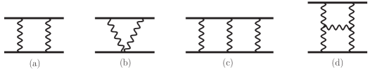
Figure 2: Examples of one- and two-loop diagram that contribute to the classical potential. Wiggly lines represent gravitons and straight lines scalars. Here the diagrams are not Feynman diagrams, but demonstrating the singularity structure from propagators in the graphs.

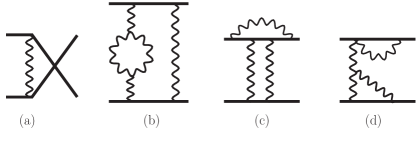
Figure 3: Examples of one- and two-loop diagrams that do not contribute to the classical potential. Wiggly lines represent gravitons and straight lines scalars. The meaning of diagrams here is the same as in Fig. 2.

A full quantum mechanical calculation of the scattering amplitude would require a proper accounting of all contributing diagrams. However, when taking the classical limit only a subset of diagrams survive and determine the contributions to the classical potential. Examples of one- and two-loop diagrams that may contain classical contributions are shown in Fig. 2. Others, such as those in Fig. 3, can be immediately discarded. By applying classical truncation at every step—from the construction of the integrand to integration—we can achieve massive simplifications, which are especially crucial for more challenging higher-loop calculations. Here we briefly outline the specific truncations we use. We will elaborate on these points substantially throughout the rest of the paper.

Following arguments that led to the absence of matter contact terms in the classical Lagrangian, an obvious contribution to discard is any diagram or part of a diagram in which matter fields come together at a local contact interaction, as illustrated at one loop in Fig. 3(a). Because the classical Lagrangian (2.1) does not contain such terms (since classical physics requires that the particles are always sufficiently separated), such contact interactions can appear only through some quantum processes, which are of no interest to us. From the perspective of generalized unitarity, this amounts to building the integrand only from those cuts that split the amplitude such that the two matter lines are on opposite sides of cut gravitons. At one loop, for example, this requirement amounts to keeping those terms that arise from the generalized unitarity cut (a) in Fig. 4, but not including any new contributions from cuts (b) or (c). In Fig. 4, there are two pairs of distinct scalars, (1,4) and (2,3), with masses $m_{1}$ and $m_{2}$.

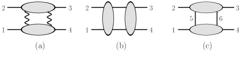
Figure 4: Generalized two-particle cuts for a elastic scattering of two distinct scalars $\phi_{1}$ and $\phi_{2}$ with masses $m_{1}$ and $m_{2}$. The pairs of legs (1,4) and (2,3) correspond to $\phi_{1}$ and $\phi_{2}$ respectively. The blobs represent tree amplitudes, which can have several diagrams in a given blob, and exposed lines are all on shell. Cut (a) separates the two matter fields by cutting graviton lines and contributes to the classical potential. The top and bottom internal lines in cut (b) are scalar $\phi_{1}$ and $\phi_{2}$, respectively. For cut (c) the internal lines are either both $\phi_{1}$ or $\phi_{2}$. Neither of the cuts (b) and (c) contains any new classical potential contributions.

Another contribution that can be discarded arises from any diagram or contribution to a diagram that contains a closed loop of momentum $\ell$ that never flows through a matter line, but only through graviton propagators, as illustrated in Fig. 3(b). The only singularities in the closed loop come from graviton poles, when $|\ell_{0}|\sim|\bm{\ell}|$, which is outside the potential region that contributes to the classical potential. Conversely, this implies that classical contributions only arise from diagrams in which all closed loops include at least one matter line. Note however that diagrams that pass this criterion may still be quantum mechanical, such as diagrams (c) and (d) in Fig. 3.

A third discarded contribution contains graviton lines which start and end on the same matter line. This implies, for example, that diagrams (c) and (d) in Fig. 3 can be discarded. One may intuitively understand this by noticing that these diagrams represent quantum mechanically-induced gravitational form factors for the matter fields. Alternatively, as we will discuss in Sec. 7, from the mechanics of integration one finds that the three-momentum component of such graviton exchanges is not parametrically set by the momentum transfer $\bm{q}$. From the perspective of generalized unitarity at one loop discarding such diagrams amounts to ignoring cuts that pass twice through the same matter line, such as the one illustrated in Fig. 4(c). In this case, the two cut internal lines are the same scalar, as identified by its mass and the Lagrangian (2.1).

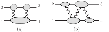
Figure 5: Some generalized unitarity cuts for extracting the conservative two-body potential at (a) 2PM order and (b) at 3PM order. The blobs represent tree amplitudes and exposed lines are all on shell. Straight lines represent massive scalars and the wiggly lines are either gluons or gravitons, depending on whether we are considering a gauge theory or a gravity cut.

As we have seen in Sec. 2.2 and will further discuss in Sec. 7, contributions to the classical potential come only from the region where internal matter lines are close to on shell or, mathematically, from regions where each energy integral is localized to a matter pole RothsteinClassical ; BjerrumClassical ; CliffIraMikhailClassical . This implies that we can effectively cut one matter line per loop. As discussed in Sec. 2.2, this is consistent with exchanged gravitons having momenta in the potential region. At one loop the net effect is that instead of using the two-particle cut in Fig. 4(a), all diagrams contributing to the classical potential are determined by generalized unitarity cut in Fig. 5(a) and its relabelings, where an additional matter line is cut, compared to Fig. 4(a). As usual, all exposed lines in the figure are placed on shell. While this provides only a modest simplification at one loop, it is much more powerful at higher loops.

Let us elaborate on how to apply the classical truncation via small $|\bm{q}|$ expansion for loop-level integrands. Recall that, as summarized in the previous sections, classical power counting implies the hierarchy of scales $m_{1},m_{2},|\bm{p}|\gg|\bm{q}|\sim|\bm{\ell}|$, where ${\bm{\ell}}$ stands for the spatial part of a generic loop momentum. We therefore scale $q\rightarrow\alpha q$ and $\ell\rightarrow\alpha\ell$ by $\alpha\sim J^{-1}\ll 1$, including the measure and propagators. For the amplitude at ${\cal O}(G^{n})$, all terms with $\alpha^{k>n-3}$ do not have classical contributions, cf. (1.2). In general, this simple scaling argument implies that terms with many powers of loop momenta in the numerators will have too high a power counting in $\alpha$ and can therefore be ignored. Such terms are responsible for the UV properties of general relativity, so it is intuitively clear that they must be quantum mechanical. For example, a consequence of this power counting is that the relevant numerators for diagrams (a) and (b) in Fig. 2 scale at most as $\alpha$ and $\alpha^{0}$, respectively. At two loops, this power counting implies that terms with more than four powers of loop momentum in any diagram numerator cannot contribute to the classical potential, and for some diagrams the bound is even tighter (see Sec. 9.2 for a related discussion). Although we keep these terms when building the integrands to make numerical cross checks easier, we drop them prior to integration to take advantage of enormous simplifications.

An important feature of this expansion is that the leading term of a diagram is not always the classical one. Rather, there exist diagrams which exhibit terms larger than the classical ones in the small $\alpha$ expansion, i.e. at ${\cal O}(G^{n})$ they scale as $\alpha^{k<n-3}$. For example, with a numerator that is independent of $q$ or $\ell$, the one-loop diagram in Fig. 2(a) scales as $\alpha^{-2}$, while that in Fig. 2(b) scales as $\alpha^{-1}$ and contributes to the classical potential. The former is an example of terms with such enhanced $\alpha$ scaling, which we refer to as “superclassical”. As we will see in Secs. 7 and 10, they have a natural interpretation as iterations of terms determined at lower orders that do not contribute directly to the classical potential at ${\cal O}(G^{n})$. They are infrared divergent and cancel in the matching between full theory and effective theory amplitudes so that the remainder is a classical contribution to the potential.

To summarize, the guidelines for efficiently applying generalized unitarity for obtaining integrands from which we can extract the classical potential are

1. Generalized unitarity cuts must separate the two matter lines to opposite sides of a cut.

2. Every independent loop must have one cut matter line.

3. Contributions where both ends of a graviton propagator attach to the same matter line are dropped.

4. Terms with too high a scaling in $q$ or $\ell$ are dropped. At two loops this implies that any term in a diagram numerator with more than four powers of loop momentum yields only quantum mechanical contributions; some diagrams require fewer loop-momentum factors.

We have confirmed these rules to be valid through two loops and will use them to organize our 3PM calculation. They determine which generalized unitarity cuts need to be included to obtain the classical potential, and which can be ignored. They also enable enormous simplifications at the integrand level by truncating away quantum contributions.

3 Building Integrands from Tree Amplitudes

3.1 General Considerations

The first step towards obtaining the classical potential is to obtain an appropriate loop integrand containing all desired classical contributions. To build the integrand we use the generalized unitarity method hep-ph/9403226 ; hep-ph/9409265 ; hep-ph/9708239 ; hep-th/0412103 ; 0705.1864 ; BRY ; BDDPR . This method meshes well with double-copy relations KLT ; BCJ ; BCJLoop that allow us to express gravity tree amplitudes and loop integrands in terms of the corresponding gauge-theory quantities. It has proven to be especially successful for carrying out high-loop computations in gravity theories, including the determination of the ultraviolet properties of extended supergravity theories at four and five loops 0905.2326 ; SimplifyingBCJ ; 1309.2498 ; 1409.3089 ; 1708.06807 ; 1804.09311 ; SimplifyingBCJ and of Einstein gravity at two loops 1507.06118 ; 1701.02422 . Further details of this methods may be found in various reviews hep-ph/9602280 ; 1103.1869 ; 1103.3298 .

The basic input into our construction are the gauge-theory tree-level scattering amplitudes collected in Appendix B. They are then converted into gravity tree amplitudes through the Kawai-Lewellen-Tye (KLT) and Bern-Carrasco-Johansson (BCJ) forms of the double copy and are subsequently used to construct generalized unitarity cuts. The KLT form of the double copy is convenient when using four-dimensional helicity states which give remarkably compact expressions for tree amplitudes. The BCJ double copy is the natural choice when organizing the calculation in terms of diagrams, as we do in our $D$-dimensional constructions.

While a purely four-dimensional approach would not lead to the correct integrand in the full quantum theory when using dimensional regularization for ultraviolet and infrared singularities, for the purpose of extracting the classical potential we shall find that four-dimensional helicity methods are sufficient. While we do encounter infrared divergences, we will see that in contrast to the full quantum theory, a simple continuation of the four-dimensional expressions to $D$ dimensions by extending the loop integration measure as well as all momentum invariants regularizes infrared singularities and does not result in any lost contributions.

While many strategies can be applied at one-loop (2PM) order, at two loops (3PM) and beyond calculations become more challenging, and require methods that scale well with increasing complexity. Our methods were designed with this in mind. For 3PM calculations both the four- and $D$-dimensional approach work well; we, however, anticipate that, given the remarkable simplicity of tree-level helicity amplitudes, as the perturbative order increases the four-dimensional helicity approach will be the method of choice. While we do not have a general proof that four-dimensional helicity states are sufficient to all orders, based on our investigations here, it seems plausible that it will continue beyond 3PM.

3.2 Building Integrands using Generalized Unitarity

The generalized unitarity method gives us a means for constructing integrands of loop-level amplitudes in terms of sums of products of tree amplitudes. Integrands are rational functions with simple poles for momentum configurations where internal lines in Feynman graphs go on shell. A propagator corresponding to such a particle is cut, i.e. it is replaced with a delta function enforcing the corresponding on-shell constraint. The residues of these poles—or generalized cuts—are given by sums of products of integrands of amplitudes whose external lines are the totality of the initial external lines and the cut lines. An important set of generalized cuts is that in which all factors are tree-level amplitudes; then, the residue is:

$$C\equiv\sum_{\rm states}A^{\rm tree}_{(1)}A^{\rm tree}_{(2)}A^{\rm tree}_{(3)}\cdots A^{\rm tree}_{(m)}\,.$$ (3.1)

We will normalize the generalized cut to be the product over the tree amplitudes that compose the cut. The sum runs over all intermediate physical states that can contribute, i.e. for which all the tree-level amplitude factors are nonvanishing. The generalized unitarity method assembles generalized cuts into complete amplitudes, by constructing a unique function whose generalized cuts reproduce those of the amplitude’s integrand. An example of generalized cut at one loop is shown in Fig. 5(a). In this figure the exposed lines are all on-shell delta functions and the blobs represent on-shell tree amplitudes. The expression for this generalized cut is given by the sum over the intermediate states of the product these two three-point amplitudes and one four-point amplitude. The full amplitude satisfies a spanning set of generalized cuts, which determine all integrands of fixed loop order and multiplicity.

The parts of amplitudes that contribute to the classical potential are determined by a rather restricted set of generalized unitarity cuts, as explained in Sec. 2.3. While the advantage may not obvious at one loop, this restriction greatly simplifies the generalized unitarity cuts at two loops.

3.3 Gravity Tree Amplitudes from the Double Copy

The generalized unitarity method is especially powerful in gravity theories because it meshes well with double-copy constructions, allowing us to express gravity amplitudes in terms of much simpler gauge-theory ones. The KLT relations KLT , which were originally derived in string theory, give us a simple means for obtaining gravity tree amplitudes in terms of color-ordered gauge-theory partial amplitudes. Through five points, which is all we need in this paper, these relations are

$$M_{3}^{\rm tree}(1,2,3) =iA_{3}^{\rm tree}(1,2,3)\,A_{3}^{\rm tree}(1,2,3)\,,$$ (3.2)

$$M_{4}^{\rm tree}(1,2,3,4) =-is_{12}A_{4}^{\rm tree}(1,2,3,4)\,A_{4}^{\rm tree}(1,2,4,3)\,,$$ (3.3)

$$M_{5}^{\rm tree}(1,2,3,4,5) =is_{12}s_{34}A_{5}^{\rm tree}(1,2,3,4,5)\,A_{5}^{\rm tree}(2,1,4,3,5)$$ (3.4)

$$\hskip 56.9055pt+is_{13}s_{24}A_{5}^{\rm tree}(1,3,2,4,5)\,A_{5}^{\rm tree}(3,1,4,2,5)\,,$$ (3.5)

where the $M_{n}^{\rm tree}$ are tree-level gravity amplitudes, the $A_{n}^{\rm tree}$ are gauge-theory partial amplitudes stripped of color factors and coupling constant, and $s_{ij}=(p_{i}+p_{j})^{2}$. We have suppressed a factor of the coupling $(\kappa/2)^{m-2}$ at $m$ points, where the coupling is given in terms of Newton’s constant via $\kappa^{2}=32\pi G$. These relations hold in any space-time dimension. An extension valid for any number of external legs may be found in Ref. MultiLegKLT .

The KLT relations are usually formulated in terms of massless amplitudes, but for the tree amplitudes used in this paper, with a single massive scalar pair, dimensional reduction shows they hold in this case as well. To show this we can start from, say, six dimensional massless gauge or gravity amplitudes and dimensionally reduce them to a four-dimensional ones with a massive scalar pair. To do so we can start with pure Yang-Mills amplitudes in, say $D=6$ and then choose the polarization vectors of legs we wish to be massive scalars, say $1$ and $2$, to be

$$\varepsilon_{1}=\varepsilon_{2}=(0,0,0,0,0,1)\,,$$ (3.6)

and their momenta to be

$$p_{1}^{A}=(p_{1}^{\mu},m,0)\,,\hskip 85.35826ptp_{2}^{A}=(p_{2}^{\mu},-m,0)\,,$$ (3.7)

where the $p_{i}^{A}$ are six dimensional momenta and $p_{i}^{\mu}$ four-dimensional ones. From the four-dimensional perspective, legs 1 and 2 are massive scalars with mass $m$ in both the gauge and gravity theories. The polarization vectors and momenta of the remaining legs live in the four-dimensional subspace specified by the first four entries. Dimensional regularization fits naturally into this framework by analytically continuing the four-dimensional subspace to $D=4-2\epsilon$ dimensions, as usual. The conclusion is that we can directly apply the KLT relations (3.5) to tree amplitudes with $n$ external gravitons two external massive scalar.

Our calculation of the part of the two-loop amplitude that contributes to the 3PM potential will require only up to five-point tree amplitudes. When evaluated using the KLT relations, the gravity tree amplitudes automatically inherit the remarkable simplicity of the gauge-theory helicity amplitudes presented in Appendix B.

A subtlety of dimensional regularization which requires careful analysis, especially beyond one-loop level and in non-supersymmetric theories, relates to finite terms of the type $\epsilon/\epsilon$, where the $1/\epsilon$ originates from an infrared singularity while the $\epsilon$ in the numerator comes from the component of loop momenta or polarization states outside four dimensions. While it seems unlikely that this could affect the classical potential, it is nevertheless important to confirm this.

To cross-check our calculation and to confirm the absence of any dimensional regularization subtleties, we also made use of BCJ form of $D$-dimensional gauge-theory tree amplitudes. While the BCJ approach generalizes to loop level integrands, here we only use it for tree-level amplitudes that enter into unitarity cuts contributing to the classical potential.

Consider an $m$-point tree-level gauge-theory scattering amplitude with all particles in the adjoint representation. We can write any such amplitude as a sum over diagrams with only cubic vertices:

$$\mathbb{A}^{{\rm tree}}_{m}=g^{m-2}\sum_{j}\frac{c_{j}n_{j}}{D_{j}}\,,$$ (3.8)

where $g$ is gauge-theory coupling constant. The denominator $1/D_{j}$ is given by the product of Feynman propagators of graph $j$. The sum runs over the $(2m-5)!!$ distinct, $m$-point graphs with only cubic vertices. Such graphs are sufficient because the contribution of any diagram with quartic vertices can be assigned to a graph with only cubic vertices by multiplying and dividing by appropriate propagators. The nontrivial kinematic information is contained in the numerators $n_{j}$, which generically depend on momenta, polarizations, and spinors. The color factor $c_{j}$ is obtained by dressing every vertex in graph $j$ with the relevant gauge-group structure constant,

$$\tilde{f}^{abc}=i\sqrt{2}f^{abc}=\mathrm{Tr}([T^{a},T^{b}]T^{c})\,,$$ (3.9)

where the gauge-group generators are normalized via $\mathrm{Tr}(T^{a}T^{b})=\delta^{ab}$, which is different than the textbook ones PeskinSchroeder , so as to be compatible with Ref. BCJ .

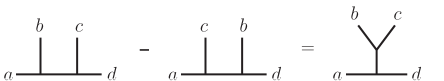
Figure 6: The Jacobi relation for a group of three graphs. The graphs can represent color factors or numerator factors and can be thought of as embedded in a larger graph.

In a BCJ representation, kinematic numerators obey the same generic algebraic relations as the color factors BCJ ; BCJLoop ; SimplifyingBCJ . For theories with only fields in the adjoint representation there are two key properties that the kinematic numerators satisfy. The first is antisymmetry under graph vertex flips:

$$c_{\overline{\imath}}=-c_{i}\ \Rightarrow\ n_{\overline{\imath}}=-n_{i}\,,$$ (3.10)

where the graph $\overline{\imath}$ has same graph connectivity as graph $i$, except an odd number of vertices have been cyclically reversed. The second property is that we require that graph numerators obey dual (kinematic) Jacobi identities whenever the color factors obey the group theoretic Jacobi identities:

$$c_{i}=c_{j}-c_{k}\ \Rightarrow\ n_{i}=n_{j}-n_{k}\,.$$ (3.11)

Here $i$, $j$, and $k$ refer to three graphs which are identical except for one internal edge, as illustrated in Fig. 6. The relative signs in the color Jacobi identity are dictated by the particular way that we drew the four-point subgraphs. For any choice, the signs of the color and kinematic Jacobi identities are identical. In general, beyond four point amplitudes, Feynman diagrams do not immediately give tree amplitudes with kinematic numerators obeying the duality. There are various systematic ways to reorganize them and manifest the duality 1010.3933 ; 1104.5224 ; 1608.00006 ; 1702.08158 ; 1703.01269 . Low-point tree amplitudes are sufficiently simple to use an ansatz to enforce desired properties, including the duality, locality and gauge invariance.

Once gauge-theory tree amplitudes or loop integrands have been arranged into a form where the duality is manifest BCJ ; BCJLoop , corresponding gravity tree amplitudes or loop integrands are given simply by replacing color factors of a the diagrams of a second gauge theory with the kinematic numerators of the first gauge-theory:

$$c_{i}\ \rightarrow\ {n}_{i}\,.$$ (3.12)

This immediately gives the double-copy form of a gravity tree amplitude,

$${M}^{{\rm tree}}_{m}=i\sum_{j}\frac{\tilde{n}_{j}n_{j}}{D_{j}}\,,$$ (3.13)

where $\tilde{n}_{j}$ and $n_{j}$ are the kinematic numerator factors of the two gauge theories. As usual we have not included factors of the gravitational coupling. In general, the two gauge theories can be distinct; since however we are interested in Einstein gravity coupled minimally to massive scalars, the two gauge theories will be identical and correspond to a Yang-Mills gauge field coupled to scalar fields in the fundamental representation Johansson:2014zca ; Johansson:2015oia ; Johansson:2019dnu . We will therefore have $\tilde{n}_{j}=n_{j}$. Since, however, we will be interested only in the double copy of tree amplitudes with two scalars, we may also take them to be in the adjoint representation.

Following the same dimensional reduction procedure as for the KLT relations, we immediately see that the double copy relations Eqs. (3.12) and (3.13) hold for the case of tree amplitudes with a single massive scalar pair and the rest being gravitons. Remarkably, these ideas extend to full integrands at loop level BCJLoop , though in this paper we will not make use of this property. We will apply the duality and double copy only for tree-level amplitudes used as input to generalized unitarity cuts.

Let us finish this section with a remark on obtaining pure Einstein gravity as a double copy. Typically the double copy of two vector fields contains more than just the graviton. For example, a gluon in four dimensions has two helicities $\pm 1$, so the square has four states: the $\pm 2$ correspond to graviton, and the zero-helicity states which are identified as the dilaton and axion. The projection to pure Einstein gravity, which eliminates the dilaton and axion, also meshes well with our generalized unitarity construction. We can simply apply the projection to graviton on each of the massless cut legs, which are external lines for tree-level blobs in a generalized unitarity cut. In any of the tree-level amplitudes, the projection on the external legs ensures that the dilaton or axion do not appear internally either, because they have to be produced in pairs when interacting with the gravitons.

In practice, we use two approaches for the graviton projection depending on the details of the unitarity construction. When using the four-dimensional helicity method, we simply correlate the helicities of the two copies of gauge theory amplitudes. For $D$-dimensional constructions, we often use the efficient projector in Eq. (5.20), as opposed to the standard one in Eq. (5.18). Such simplification is made possible by choosing a special form of tree-level amplitudes in gauge theory. See the discussion in Sec. 5.

4 Integrands at One Loop Using Four-Dimensional Helicity

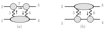
Figure 7: The two generalized unitarity cuts for extracting the conservative two-body potential at 2PM order. The blobs represent tree amplitudes and exposed lines are all on shell. Straight lines represent massive scalars and the wiggly lines are either gluons or gravitons, depending on whether we are considering a gauge theory or a gravity cut.

To illustrate some essential features of our procedure for constructing amplitudes’ integrands in the post-Minkowskian expansion, we first describe the 2PM order, discussed earlier in Refs. Westpfahl2PM ; CachazoGuevara ; DamourTwoLoop ; BjerrumClassical ; CliffIraMikhailClassical ; Paolo2PM ; Cristofoli:2019neg ; 1905.05657 ; 1906.05209 . As discussed in Sec. 2, the part of loop integrands that contributes to the classical potential is determined by a restricted set of generalized unitarity cuts: they separate the two matter lines and also they place on shell one matter line per loop RothsteinClassical ; BjerrumClassical ; CliffIraMikhailClassical . Thus, at one loop, corresponding to the 2PM case, we need only compute the two generalized cuts illustrated in Fig. 7.

At one-loop the cuts can be evaluated in various ways. In particular, the calculation is not simplified substantially by making use of on-shell conditions on the matter lines. Similarly, its complexity is not affected much by judicious choices for the graviton physical state projector. Beyond one loop, however, care is necessary to ensure that the calculation scales well CliffIraMikhailClassical ; 3PMPRL . This includes adjusting the tree-level amplitude factors so that the physical-state projectors trivialize and also making sure that on-shell conditions are used to their maximal extent. Therefore, to illustrate all subtleties of the amplitudes’ construction, in our one-loop calculation below we will make use of the cut conditions on the matter lines, even though it causes the slight additional complication that different cuts double count certain terms. This must be taken into account when the cuts are combined into a single integrand. Such double counts are natural beyond one loop, so the one-loop case offers a simple illustration of this issue and its resolution.

4.1 Warm-up: Gauge-Theory Integrands

As a warm-up, we consider gauge theory and construct the one-loop integrand for the classical potential between two massive scalars due to gluon exchange. As we shall see, once we have the gauge-theory integrand, obtaining the gravity one is quite straightforward.

We first evaluate the generalized cut in Fig. 7(a), for the case of a one-loop color-ordered YM amplitude. In color-ordered amplitudes the external legs follow a cyclic ordering and are stripped of color factors. This generalized cut is,

$$C_{\rm YM}^{\rm(a)} =\sum_{h_{5},h_{6}=\pm}A^{\rm tree}_{3}(3^{s},6^{h_{6}},-7^{s})\,A^{\rm tree}_{3}(7^{s},-5^{h_{5}},2^{s})\,A^{\rm tree}_{4}(1^{s},5^{-h_{5}},-6^{-h_{6}},4^{s})\,,$$ (4.1)

where $\pm$ superscripts denote the gluon helicity and $s$ stands for scalar, and the minus sign on the label indicates that the sign of the momentum should be reversed when treated as an outgoing momentum of the amplitude. The state sum runs over the gluon helicities. Since each propagating scalar corresponds to a single state there is no sum associated with it. In four dimensions each gluon can either be of positive or negative helicity, giving a total of four helicity configurations in the state sum. We label them as follows:

$$\{h_{5},h_{6}\}:\;\;\{++\},\;\{--\},\;\{-+\},\;\{+-\}\,,$$ (4.2)

where the helicities of the gluon legs are labeled with an outgoing momentum convention. In $D$ dimensions each gluon has $D-2$ states. At one-loop we will evaluate the cuts in four dimensions and compare it to the result obtained via $D$-dimensional methods. We show that the two methods give same four-dimensional classical potential.

The four-point tree amplitudes appearing in the cut (4.1) are given in Eq. (B.1). One may evaluate the product of three-point tree amplitudes appearing in cuts by starting from Feynman three-point vertices and evaluating them on helicity states. Alternatively, we may extract their product from the four-point amplitude (B.1), by removing the scalar propagator and placing its momentum on shell. Below we use the second approach.

Starting with the two-scalar two-gluon amplitude in Eq. (B.1) with the gluons in the $\{++\}$ helicity configuration and removing the scalar propagator $i/\tau_{36}$ we have

$$A^{\rm tree}_{3}(3^{s},6^{+},-5^{+},2^{s})\rightarrow A^{\rm tree}_{3}(3^{s},6^{+},-7^{s})\,A^{\rm tree}_{3}(7^{s},-5^{+},2^{s})=\frac{m_{2}^{2}\left[-5\,6\right]}{\left\langle-5\,6\right\rangle}\,,$$ (4.3)

where we use the helicity notation of Ref. hep-th/0509223 ; hep-ph/9601359 . For simplicity, we only keep the momentum label in spinor expressions, e.g. $\left[-5\,6\right]\equiv\left[(-\ell_{5})\,\ell_{6}\right]$. Using the on shell condition for that propagator, $p_{3}\cdot\ell_{6}=0$, the cut for the $\{++\}$ helicity configuration is

$$C_{\rm YM}^{\{++\}} =A^{\rm tree}_{3}(3^{s},6^{+},-7^{s})\,A^{\rm tree}_{3}(7^{s},-5^{+},2^{s})\,A^{\rm tree}_{4}(1^{s},5^{-},-6^{-},4^{s})$$

$$=i\frac{m_{2}^{2}\left[-5\,6\right]}{\left\langle-5\,6\right\rangle}\,\frac{m_{1}^{2}\left\langle-6\,5\right\rangle}{\left[-6\,5\right]\,\tau_{15}}$$

$$=i\frac{m_{1}^{2}m_{2}^{2}}{\tau_{15}}\,,$$ (4.4)

where

$$\tau_{ij}=2p_{i}\cdot\ell_{j}\,,$$ (4.5)

and we again used the two-scalar two-gluon amplitude in Eq. (B.1) for the second four-point amplitude in the cut.

Similarly, for the $\{--\}$ helicity configuration we obtain the same expression,

$$C_{\rm YM}^{\{--\}} =A^{\rm tree}_{3}(3^{s},6^{-},-7^{s})\,A^{\rm tree}_{3}(7^{s},-5^{-},2^{s})\,A^{\rm tree}_{4}(1^{s},5^{+},-6^{+},4^{s})$$

$$=i\frac{m_{1}^{2}m_{2}^{2}}{\tau_{15}}\,.$$ (4.6)

Next consider the $\{-+\}$ helicity configuration. Evaluating it along the same lines of taking the residue of the $\tau_{36}$ pole of a two-particle cut and evaluating the result at $\tau_{36}=0$, we find

$$C_{\rm YM}^{\{-+\}} =A^{\rm tree}_{3}(3^{s},6^{+},-7^{s})\,A^{\rm tree}_{3}(7^{s},-5^{-},2)\,A^{\rm tree}(1^{s},5^{+},-6^{-},4^{s})$$

$$=i\frac{\left\langle-5{\vphantom{1}}\right|{{2}}\left|6\right]^{2}}{(\ell_{5}-\ell_{6})^{2}}\times\frac{\left\langle-6{\vphantom{1}}\right|{{4}}\left|5\right]^{2}}{(\ell_{5}-\ell_{6})^{2}\tau_{15}}$$

$$=\frac{i}{t^{2}}\frac{{\rm tr}_{+}^{2}[5462]}{\tau_{15}}\,,$$ (4.7)

where $t\equiv(p_{2}+p_{3})^{2}=(\ell_{5}-\ell_{6})^{2}$ and

$${\rm tr}_{\pm}[abcd]\equiv\frac{1}{2}{\rm tr}[abcd]\pm\frac{1}{2}{\rm tr}_{5}[abcd]\equiv\frac{1}{2}{\rm tr}[(1\pm\gamma_{5}){\raise-0.34723pt\hbox to5.28589pt{\hss/\hss}\hbox to0.0pt{\hss$a$}}{\raise 0.97221pt\hbox to4.29166pt{\hss/\hss}\hbox to0.0pt{\hss$b$}}{\raise-0.34723pt\hbox to4.32756pt{\hss/\hss}\hbox to0.0pt{\hss$c$}}{\raise 0.97221pt\hbox to5.20486pt{\hss/\hss}\hbox to0.0pt{\hss$d$}}]\,.$$ (4.8)

The $\{+-\}$ helicity configuration is identical except we have to switch angle and square brackets, which has the effect of interchanging a ${\rm tr}_{-}$ and a ${\rm tr}_{+}$. This gives

$$\hskip 28.45274ptC_{\rm YM}^{\{+-\}} =A^{\rm tree}_{3}(3^{s},6^{-},-7^{s})\,A^{\rm tree}_{3}(7^{s},-5^{+},2)\,A^{\rm tree}_{4}(1,5^{-},-6^{+},4)$$

$$=\frac{i}{t^{2}}\frac{{\rm tr}_{-}^{2}[5462]}{\tau_{15}}\,.$$ (4.9)

The parity odd terms cancel, as expected, after summing the $\{-+\}$ and $\{+-\}$ helicities configurations in Eqs. (4.7) and (4.9).

Summing over the four helicity contributions in Eqs. (4.4), (4.6), (4.7) and (4.9) to the cut in Fig. 7(a) and simplifying the resulting expression, we find

$$C_{\rm YM}^{\rm(a)} =C_{\rm YM}^{\{++\}}+C_{\rm YM}^{\{--\}}+C_{\rm YM}^{\{-+\}}+C_{\rm YM}^{\{+-\}}$$

$$=\frac{i}{\tau_{15}}\Bigl{(}\frac{1}{t^{2}}({\rm tr}_{+}^{2}[5462]+{\rm tr}_{-}^{2}[5462])+2m_{1}^{2}m_{2}^{2}\Bigr{)}\,.$$ (4.10)

The cut in Fig. 7(b) is given by a simple relabeling, $(1,4)\leftrightarrow(2,3)$, $5\rightarrow-5$ and $6\rightarrow-6$,

$$C_{\rm YM}^{\rm(b)} =\frac{i}{\tau_{36}}\Bigl{(}\frac{1}{t^{2}}({\rm tr}_{+}^{2}[5163]+{\rm tr}_{-}^{2}[5163])+2m_{1}^{2}m_{2}^{2}\Bigr{)}$$

$$=\frac{i}{\tau_{36}}\Bigl{(}\frac{1}{t^{2}}({\rm tr}_{+}^{2}[5462]+{\rm tr}_{-}^{2}[5462])+2m_{1}^{2}m_{2}^{2}\Bigr{)}\,,$$ (4.11)

where in the second equal sign we used that $p_{2}=-p_{3}+\ell_{5}-\ell_{6}$ and $p_{4}=-p_{1}-\ell_{5}+\ell_{6}$ and that legs $5$ and $6$ are on shell.

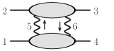
Figure 8: The two particle cut at one loop containing classical potential. The blobs represent tree amplitudes and exposed lines are all on shell.

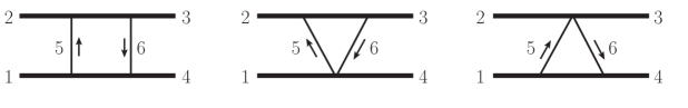
Figure 9: The one-loop box and triangle integrals. The top and bottom thick lines are massive scalars $1$ and $2$, respectively, and the thin lines are massless.

The last step in the construction of the integrand requires that we combine the two cuts in Fig. 7, with values given in Eqs. (4.10) and (4.11), into a single function. This needs to be done such that any double counting coming from the same terms appearing in both cuts is eliminated. At two loops we will do this by constructing an ansatz whose generalized cuts are constrained to match all required cuts. At one loop such an approach is overly laborious. The overlap can be more easily seen by inspection. Because the two cuts have identical numerator factors, it is straightforward to construct a function which reduces to Eqs. (4.10) and (4.11) upon imposing cut conditions on one of the propagators $i/\tau_{15}$ and $i/\tau_{36}$, respectively. It is

$$C_{\rm YM} =-\frac{1}{\tau_{15}\tau_{36}}\Bigl{(}\frac{1}{t^{2}}({\rm tr}_{+}^{2}[5462]+{\rm tr}_{-}^{2}[5462])+2m_{1}^{2}m_{2}^{2}\Bigr{)}\,.$$ (4.12)

It is worth stressing that this function needs not a priori be (and in fact it is not) the two-gluon cut of the one-loop four-scalar amplitude displayed in Fig. 8 because it may not contain all terms from which $1/\tau_{15}$ and $1/\tau_{36}$ are absent, corresponding to a graviton bubble connected to the matter lines. It however does capture, by construction, all the box and triangle contributions to the one-loop amplitude, which are the parts needed for the extraction of the classical limit of the amplitude. See Fig. 9 for the diagrams that correspond to the box and triangle integrals.

Restoring the loop integration and the graviton propagators while relaxing the on shell condition for their momenta gives the part of the one-loop amplitude which contributes in the classical limit of the gauge-theory four-scalar amplitude:

$$A^{{\rm 1\hbox{-}loop}}_{4} =\int\frac{d^{D}\ell_{5}}{(2\pi)^{D}}\,\frac{N_{\rm YM}}{\ell_{5}^{2}((\ell_{5}-p_{2})^{2}-m_{2}^{2})(\ell_{5}-p_{2}-p_{3})^{2}((\ell_{5}+p_{1})^{2}-m_{1}^{2})}\,.$$ (4.13)

This last step does not capture terms in which either one or both graviton propagators are canceled; while such terms do appear in the complete quantum amplitude, which we discuss in Sec. 12.1, they do not contribute to its classical limit because they correspond to contact rather than long-distance interaction of the matter fields. The gauge-theory numerator is

$$N_{\rm YM}=\frac{1}{t^{2}}({\rm tr}_{+}^{2}[5462]+{\rm tr}_{-}^{2}[5462])+2m_{1}^{2}m_{2}^{2}\,.$$ (4.14)

We also promoted the integration measure to $D=4-2\epsilon$ dimensions, dimensionally regularizing the infrared divergences of the amplitude.

We can simplify somewhat Eq. (4.14) by evaluating the $\gamma$-traces. Using standard $\gamma$-matrix identities, they evaluate to

$${\rm tr}_{\pm}[5462] ={\cal E}\pm{\cal O}\,,$$ (4.15)

where the parity even part is

$${\cal E} =\frac{1}{2}{\rm tr}[5462]$$

$$=2\ell_{5}\cdot p_{4}\ell_{6}\cdot p_{2}-2\ell_{5}\cdot\ell_{6}p_{4}\cdot p_{2}+2\ell_{5}\cdot p_{2}\ell_{6}\cdot p_{4}$$

$$=\frac{1}{2}\Bigl{(}-st+tm_{1}^{2}+tm_{2}^{2}+t\,\tau_{15}+t\tau_{36}+2\tau_{15}\tau_{36}\Bigr{)}\,,$$ (4.16)

which we simplified using the graviton cut conditions. The parity odd part is

$${\cal O}=2i\varepsilon_{\mu\nu\rho\sigma}\ell_{5}^{\mu}p_{4}^{\nu}\ell_{6}^{\rho}p_{2}^{\sigma}\,.$$ (4.17)

This term integrates to zero because there are insufficient independent external momenta to saturate all the indices of the Levi-Civita symbol. While the parity-odd term cancels between the two traces in Eq. (4.14),

$${\rm tr}_{-}^{2}[5462]+{\rm tr}_{+}^{2}[5462]=2({\cal E}^{2}+{\cal O}^{2})\,,$$ (4.18)

its square does not; it gives a Gram determinant,

$${\cal O}^{2} =G_{4}\equiv 4\det\left(\begin{matrix}\ell_{5}\cdot\ell_{5}&\ell_{5}\cdot p_{4}&\ell_{5}\cdot\ell_{6}&\ell_{5}\cdot p_{2}\\ p_{4}\cdot\ell_{5}&p_{4}\cdot p_{4}&p_{4}\cdot\ell_{6}&p_{4}\cdot p_{2}\\ \ell_{6}\cdot\ell_{5}&\ell_{6}\cdot p_{4}&\ell_{6}\cdot\ell_{6}&\ell_{6}\cdot p_{2}\\ p_{2}\cdot\ell_{5}&p_{2}\cdot p_{4}&p_{2}\cdot\ell_{6}&p_{2}\cdot p_{2}\end{matrix}\right).$$ (4.19)

After being evaluated and simplified it becomes

$${\cal O}^{2}={\cal E}^{2}-(tm_{1}^{2}+t\,\tau_{15}+\tau_{15}^{2})(tm_{2}^{2}+t\,\tau_{36}+\tau_{36}^{2})\,,$$ (4.20)

with ${\cal E}^{2}$ being the square of eq. (4.16).

We can rewrite the numerator (4.14) in terms of Mandelstam variables via Eq. (4.18)

$$N_{\rm YM}=\frac{2}{t^{2}}\left({\cal E}^{2}+{\cal O}^{2}\right)+2m_{1}^{2}m_{2}^{2}\,,$$ (4.21)

where ${\cal E}^{2}$ and ${\cal O}^{2}$ can be found from Eqs. (4.16) and (4.20). After inserting this into Eq. (4.13) and keeping only the box and triangle integrals, as shown in Fig. 9, we find that the one-loop four scalar amplitude is

$$A^{{\rm 1\hbox{-}loop}}_{4} =\int\frac{d^{D}\ell_{5}}{(2\pi)^{D}}\,\frac{1}{\ell_{5}^{2}(\ell_{5}-p_{1}-p_{2})^{2}}\biggl{[}\frac{(s-m_{1}^{2}-m_{2}^{2})^{2}}{((\ell_{5}+p_{1})^{2}-m_{1}^{2})\,((\ell_{5}-p_{2})^{2}-m_{2}^{2})}$$ (4.22)

$$\hbox{}\hskip 56.9055pt+\frac{2m_{1}^{2}t-2m_{2}^{2}\tau_{15}+\tau_{15}t-2st}{((\ell_{5}-p_{2})^{2}-m_{2}^{2})\,t}+\frac{2m_{2}^{2}t-2m_{1}^{2}\tau_{36}+\tau_{36}t-2st}{((\ell_{5}+p_{1})^{2}-m_{1}^{2})\,t}\biggr{]}+\hbox{quantum}\,.$$

The integrals are to be evaluated in $D=4-2\epsilon$ dimensions.

Given that the integrand of Eq. (4.22) is determined in four dimensions, yet when integrated it is infrared divergent, one might worry that ${\cal O}(\epsilon)$ terms which are dropped from the integrand may actually contribute when multiplied by an infrared divergence. In the full quantum theory a four-dimensional integrand evaluation would miss certain rational pieces, as it happens in QCD BernMorgan . However, as we shall see in Sec. 12.2, for extracting the classical potential it is sufficient to evaluate the integrand in four dimensions not only at one loop, but also at two loops.

4.2 Gravity Integrands

Using the double copy we now convert the above gauge-theory results for the integrand into a corresponding gravity integrand. Given the simplicity of the gauge-theory helicity amplitudes, it is natural to apply the KLT relations (3.5) for tree amplitudes in the cuts. This strategy is used in Ref. BjerrumQuantum to study PN and quantum corrections to the Newtonian potential.

Using the KLT relations, the generalized unitarity cut in Fig. 7(a) for the gravity amplitude is

$$C_{\rm GR}^{\rm(a)} =\sum_{h_{5},h_{6}=\pm}M^{\rm tree}_{3}(3^{s},6^{h_{6}},-7^{s})\,M^{\rm tree}_{3}(7^{s},-5^{h_{5}},2^{s})\,M^{\rm tree}_{4}(1^{s},5^{-h_{5}},-6^{-h_{6}},4^{s})$$

$$=\sum_{h_{5},h_{6}=\pm}it[A^{\rm tree}_{3}(3^{s},6^{h_{6}},-7^{s})\,A^{\rm tree}_{3}(7^{s},-5^{h_{5}},2^{s})\,A^{\rm tree}_{4}(1^{s},5^{-h_{5}},-6^{-h_{6}},4^{s})]$$

$$\hskip 56.9055pt\hbox{}\times[A^{\rm tree}_{3}(3^{s},6^{h_{6}},-7^{s})\,A^{\rm tree}_{3}(7^{s},-5^{h_{5}},2^{s})\,A^{\rm tree}_{4}(4^{s},5^{-h_{5}},-6^{-h_{6}},1^{s})]\,,$$ (4.23)

where we use the BCJ amplitude relation BCJ

$$s_{12}A^{\rm tree}(1,2,4,3)=s_{23}A^{\rm tree}(4,2,3,1)\,,$$ (4.24)

for all four-point tree amplitudes in this paper. So, in the end, the gravity cut is expressed directly in terms of the four helicity components of the gauge-theory cut. We project out the dilaton and axion ubiquitous in the double-copy relations and enforce that only gravitons propagate across cuts simply by correlating the helicities in the two gauge-theory copies. As in the gauge-theory calculation, some care is needed to ensure that the difference between $D$ and four dimensions does not affect the classical limit which we discuss in Sec. 12.2.

Following the gauge-theory analysis, we step, one by one, through the four helicity configurations (4.2) of the cut gravitons. For the $\{++\}$ configuration we have

$$C_{\rm GR}^{\rm\{++\}} =M^{\rm tree}_{3}(3^{s},6^{+},-7^{s})\,M^{\rm tree}_{3}(7^{s},-5^{+},2^{s})\,M^{\rm tree}(1,5^{-},-6^{-},4)$$

$$=it\,[A^{\rm tree}_{3}(3^{s},6^{+},-7^{s})\,A^{\rm tree}_{3}(7^{s},-5^{+},2^{s})\,A^{\rm tree}_{4}(1,5^{-},-6^{-},4^{s})]$$

$$\hskip 21.62393pt\hbox{}\times[A^{\rm tree}_{3}(3^{s},6^{+},-7^{s})\,A^{\rm tree}_{3}(7^{s},-5^{+},2^{s})\,A^{\rm tree}_{4}(4,5^{-},-6^{-},1^{s})]\,.$$ (4.25)

We simply read off the answer from the YM result in Eq. (4.4) after appropriate relabeling. It is

$$C_{\rm GR}^{\{++\}} =-it\frac{m_{1}^{2}m_{2}^{2}}{\tau_{15}}\,\frac{m_{1}^{2}m_{2}^{2}}{\tau_{45}}\,.$$ (4.26)

We partial fraction the product of propagators, to make it compatible with a diagrammatic interpretation,

$$\frac{1}{\tau_{15}\tau_{45}} =-\frac{1}{t}\Bigl{(}\frac{1}{\tau_{15}}+\frac{1}{\tau_{45}}\Bigr{)}\,,$$ (4.27)

where $t=(\ell_{5}-\ell_{6})^{2}=(p_{1}+p_{4})^{2}$. In carrying out this partial fractioning we use the fact that $\ell_{5}$ and $\ell_{6}$ are on-shell momenta and, as in the gauge-theory evaluation of cuts, we have an all-outgoing convention for external momenta. The momentum flow of $\ell_{5}$ and $\ell_{6}$ is indicated in Fig. 7. This gives the remarkably simple result for the generalized cut with the $\{++\}$ helicity configuration,

$$C_{\rm GR}^{\{++\}}=im_{1}^{4}m_{2}^{4}\Bigl{(}\frac{1}{\tau_{15}}+\frac{1}{\tau_{45}}\Bigr{)}\,.$$ (4.28)

As for gauge theory, the result for the $(--)$ helicity configuration is identical to that of the $\{++\}$ configuration:

$$C_{\rm GR}^{\{--\}}=im_{1}^{4}m_{2}^{4}\Bigl{(}\frac{1}{\tau_{15}}+\frac{1}{\tau_{45}}\Bigr{)}\,.$$ (4.29)

Next, we evaluate the cut with the $\{-+\}$ helicity configuration for the cut gravitons. We obtain

$$C_{\rm GR}^{\{-+\}}= M^{\rm tree}_{3}(3^{s},6^{+},-7^{s})\,M^{\rm tree}_{3}(7^{s},-5^{-},2^{s})\,M^{\rm tree}_{4}(1^{s},5^{+},-6^{-},4^{s})$$

$$= it\,[A^{\rm tree}_{3}(3^{s},6^{+},-7^{s})\,A^{\rm tree}_{3}(7^{s},-5^{-},2^{s})\,A^{\rm tree}_{4}(1^{s},5^{+},-6^{-},4^{s})]$$

$$\quad\times[A^{\rm tree}_{3}(3^{s},6^{+},-7^{s})\,A^{\rm tree}_{3}(7^{s},-5^{-},2^{s})\,A^{\rm tree}_{4}(4^{s},5^{+},-6^{-},1^{s})]\,.$$ (4.30)

Reading off the YM result in Eq. (4.7) and appropriately relabeling, we find

$$C_{\rm GR}^{\rm(-+)} =-\frac{i}{t^{3}}\frac{{\rm tr}_{-}^{2}[5462]}{\tau_{15}}\,\frac{{\rm tr}_{-}^{2}[5462]}{\tau_{45}}\,.$$ (4.31)

In addition, partial fractioning the product of propagators using Eq. (4.27) gives

$$C_{\rm GR}^{\rm(-+)}= \frac{i}{t^{4}}{\rm tr}_{-}^{4}[5462]\,\Bigl{(}\frac{1}{\tau_{15}}+\frac{1}{\tau_{45}}\Bigr{)}\,.$$ (4.32)

Following similar steps for the final $(+-)$ helicity configuration (or simply conjugating the result for the $\{-+\}$ configuration), we have

$$C_{\rm GR}^{\rm(+-)}= \frac{i}{t^{4}}{\rm tr}_{+}^{4}[5462]\,\Bigl{(}\frac{1}{\tau_{15}}+\frac{1}{\tau_{45}}\Bigr{)}\,.$$ (4.33)

Combining Eqs. (4.28), (4.29), (4.32) and (4.33) yields the cut in Fig. 7(a):

$$C_{\text{GR}}^{\rm(a)} =C_{\rm GR}^{\rm(++)}+C_{\rm GR}^{\rm(--)}+C_{\rm GR}^{\rm(-+)}+C_{\rm GR}^{\rm(+-)}$$

$$=i\Bigl{(}\frac{1}{t^{4}}\,\bigl{(}{\rm tr}_{-}[5462]^{4}+{\rm tr}_{+}[5462]^{4}\bigr{)}+2m_{1}^{4}m_{2}^{4}\Bigr{)}\Bigl{(}\frac{1}{\tau_{15}}+\frac{1}{\tau_{45}}\Bigr{)}\,.$$ (4.34)

Again the parity odd terms cancel in the integrand between the contributions of the various helicity configurations. We obtain the second required cut, shown in Fig. 7(b), by a simple relabeling and applying on-shell conditions, as in the gauge-theory case:

$$C_{\text{GR}}^{\rm(b)} =i\Bigl{(}\frac{1}{t^{4}}\,\bigl{(}{\rm tr}_{-}[5462]^{4}+{\rm tr}_{+}[5462]^{4}\bigr{)}+2m_{1}^{4}m_{2}^{4}\Bigr{)}\Bigl{(}\frac{1}{\tau_{36}}+\frac{1}{\tau_{26}}\Bigr{)}\,.$$ (4.35)

Relaxing the on-shell condition for the cut momenta, restoring the cut propagators and combining Eqs. (4.34) and (4.35) into a single expression whose two cuts in Fig. 7 match Eqs. (4.34) and (4.35) leads to

$$M^{\rm 1\hbox{-}loop}(1,2,3,4) =\frac{1}{2}\int\frac{d^{D}\ell_{5}}{(2\pi)^{D}}\,N_{\rm GR}\,\biggl{[}\frac{1}{\ell_{5}^{2}((\ell_{5}-p_{2})^{2}-m_{2}^{2})(\ell_{5}-p_{2}-p_{3})^{2}((\ell_{5}+p_{1})^{2}-m^{2})}$$

$$\hskip 113.81102pt+\{2\leftrightarrow 3\}+\{1\leftrightarrow 4\}+\{2\leftrightarrow 3,1\leftrightarrow 4\}\biggr{]}+\hbox{quantum}\,,$$ (4.36)

where $\ell_{6}=\ell_{5}-p_{2}-p_{3}$ and we included an overall 1/2 for the two-graviton phase-space symmetry factor. The numerator $N_{\rm GR}$ is

$$N_{\rm GR} =\frac{1}{t^{4}}\,({\rm tr}_{-}^{4}[5462]+{\rm tr}_{+}^{4}[5462])+2m_{1}^{4}m_{2}^{4}$$

$$=\frac{2}{t^{4}}\,(({\cal E}^{2}+{\cal O}^{2})^{2}+4{\cal E}^{2}{\cal O}^{2})+2m_{1}^{4}m_{2}^{4}\,,$$ (4.37)

where ${\cal E}^{2}$ and ${\cal O}^{2}$ can be found from Eqs. (4.16) and (4.20). The numerator is symmetric under the relabelings indicated in Eq. (4.36). We see that each integral appears twice, and we can simplify the amplitude (4.36) to

$$M^{\rm 1\hbox{-}loop}(1,2,3,4) =\int\frac{d^{D}\ell_{5}}{(2\pi)^{D}}\,N_{\rm GR}\biggl{[}\frac{1}{\ell_{5}^{2}((\ell_{5}-p_{2})^{2}-m_{2}^{2})(\ell_{5}-p_{2}-p_{3})^{2}((\ell_{5}+p_{1})^{2}-m_{1}^{2})}$$

$$\hskip 85.35826pt+\{1\leftrightarrow 4\}\Bigr{]}+\hbox{quantum}\,.$$ (4.38)

This immediately can be reduced to the standard scalar box, triangle and bubble integrals. The bubble integrals are all quantum and can be dropped without affecting the classical potential. The box integral is obtained by setting $\tau_{15},\tau_{36}\rightarrow 0$ since these factors cancel matter propagators that would give us triangle or bubble integrals. This gives us the box-integral contribution

$$-t^{2}(M_{4}^{\rm tree})^{2}\int\frac{d^{D}\ell_{5}}{(2\pi)^{D}}\,\frac{1}{\ell_{5}^{2}((\ell_{5}-p_{2})^{2}-m_{2}^{2})(\ell_{5}-p_{2}-p_{3})^{2}}\biggl{(}\frac{1}{(\ell_{5}+p_{1})^{2}-m_{1}^{2}}+\frac{1}{(\ell_{5}+p_{4})^{2}-m_{1}^{2}}\biggr{)}\,,$$ (4.39)

where the four-dimensional tree amplitude is

$$M_{4}^{\rm tree}=-i\,\frac{(s-m_{1}^{2}-m_{2}^{2})^{2}-2m_{1}^{2}m_{2}^{2}}{t}\,.$$ (4.40)

The appearance of the square of the tree amplitude in front of the box integral is not an accident and is intimately connected to the fact that, from the effective field theory perspective, the box contribution is an infrared-divergent iteration of tree-level exchange. This will be subtracted in matching with effective field theory and will not have an independent contribution to the classical potential.

As a simple check, it is not difficult to add back the dilaton and axion (antisymmetric tensor) contributions. To get these we simply sum over the contributions where, for at least one cut leg, the helicities of two gluons corresponding to a particle in the double copy theory are anti-correlated. Repeating the above steps for this case then gives the dilaton and axion contributions to the numerator,

$$N_{\rm\phi a}=\frac{1}{t^{4}}\,\bigl{(}2{\rm tr}_{+}^{2}[5462]\,{\rm tr}_{-}^{2}[5462]\bigr{)}+2m_{1}^{4}m_{2}^{4}+\frac{4}{t^{2}}\bigl{(}{\rm tr}_{+}^{2}[5462]+{\rm tr}_{-}^{2}[5462]\bigr{)}m_{1}^{2}m_{2}^{2}\,.$$ (4.41)

Combining the graviton contribution to the numerator (4.37), with that of the dilaton and axion (4.41) gives exactly the simple double-copy form for the numerator,

$$N_{\rm GR}+N_{\rm\phi a} =\Bigl{(}\frac{{\rm tr}_{+}^{2}[5462]+{\rm tr}_{-}^{2}[5462]}{t^{2}}+2m_{1}^{2}m_{2}^{2}\Bigr{)}^{2},$$ (4.42)

which is the square of the gauge-theory numerator in Eq. (4.14), as expected.

Although we calculated the integrand in four dimensions, the result in Eq. (4.38) is perfectly valid for extracting the classical potential, despite of the fact that we will use dimensional regularization to regularize infrared divergences. The details can be found in Sec. 12.2.

5 Integrands at One Loop Using $D$-Dimensional Methods

When constructing scattering amplitudes we encounter infrared-divergent integrals. To evaluate them we use dimensional regularization, where we continue the space-time dimension from four to $D=4-2\epsilon$. Infrared singularities appear as poles in $\epsilon$, which can interfere with ${\cal O}(\epsilon)$ terms to produce finite contributions. Indeed, in the full quantum theory such terms do occur and need to be kept, as described in e.g. Ref. BernMorgan . We therefore need to confirm that ${\cal O}(\epsilon)$ terms in the integrand do not alter our results for the classical potential in some way.

When applying dimensional regularization, the simplest scheme is the so-called conventional dimensional regularization (CDR) scheme CDR , where all states and loop momenta are analytically continued from four to $D$ dimensions. The four-dimensional helicity (FDH) scheme Bern:1991aq ; hep-ph/0202271 is an alternative that meshes well with helicity methods. In this scheme, we distinguish between the dimension of loop momenta and the space where physical states live. We treat any factor of $D$ arising in the integrand from contracting Lorentz indices, $D_{s}=\eta_{\mu}^{\ \mu}=4$, differently from loop momenta which we take to live in $D=4-2\epsilon$. We find it useful to distinguish between these two sources of dimension dependence to help track how dependence on the dimensional regularization prescriptions drop out in the classical potential, as discussed in Sec. 12.2. While a technical point, this is of some importance, especially beyond two loops where four-dimensional helicity methods, which implicitly choose both $D=4$ and $D_{s}=4$, are expected to be more efficient than $D$-dimensional ones.

In this section, as a warm-up for the more complicated two-loop case, we investigate the dependence on regularization scheme by constructing a $D$-dimensional version of the one-loop integrand which we compare to the one obtained in Sec. 4 using four-dimensional methods. Such a $D$-dimensional one-loop integrand has also been recently constructed using similar methods in Ref. Paolo2PM . The one-loop case is especially simple because, as we shall see, the $D$- and four-dimensional integrands are identical up to differences in the $D_{s}$ state-counting parameters. As we discuss in Sec. 6, at two loops the difference is nontrivial because of the appearance of Gram determinants of momentum invariants that vanish in four dimensions but not in $D>4$ dimensions. Nevertheless, we will show that they do not affect the classical potential.

5.1 Warm-up: Gauge-Theory Integrands

Our $D$-dimensional construction makes use of BCJ duality, reviewed in Sec. 3, so it is natural to start with color-dressed amplitudes, instead of color-ordered ones. As in the four-dimensional discussion, once we obtain a $D$-dimensional gauge-theory integrand, the double-copy construction gives the gravitational one with minimal additional effort.

An essential component of the evaluation of generalized unitarity cuts is the sum over physical states. At two loops they can become quite involved so it is useful to devise methods for simplifying them. The sum over the physical states of a gluon in general dimension is less straightforward than summing over positive and negative helicities in four dimensions. It is given by the so-called physical state projector,

$$P^{\mu\nu}(p,q)=\sum_{\rm pols.}\varepsilon^{\mu}(-p)\varepsilon^{\nu}(p)=\eta^{\mu\nu}-{q^{\mu}p^{\nu}+p^{\mu}q^{\nu}\over q\cdot p}\,,$$ (5.1)

where the sum runs over the physical gluon polarizations, $p$ is the gluon momentum and $q$ is an arbitrary null reference momentum. We can use the projector to replace a pair of polarization vectors with kinematic invariants. Note that there is a spurious propagator, $1/q\cdot p$, which must cancel out once all on-shell conditions on the cut are applied.

While including this projector in one-loop unitarity cuts poses no technical challenges, by two loops using it becomes cumbersome, especially for gravity. However, as we now explain, we can adjust the form of the tree amplitudes to automatically set to zero all terms that depend on the reference momentum. The essential idea is to choose a form of the tree-level amplitudes used in cuts such that, when a polarization vector is replaced by the corresponding momentum (i.e. under a gauge transformation), the amplitude vanishes without using the transversality of the remaining polarization vectors Paolo2PM . This significantly cleans up $D$-dimensional unitarity cuts beyond one loop because it allows us to use a simpler physical state projector.

To illustrate this idea, we start with the three-point tree amplitude with one gluon and two massive scalars in the adjoint representation. It is given by the Feynman three-point vertex,

$$\mathbb{A}_{3}^{\rm tree}(1^{s},2,3^{s})=\frac{i}{\sqrt{2}}\,\tilde{f}^{a_{1}a_{2}a_{3}}(p_{3}-p_{1})\cdot\varepsilon_{2}\,.$$ (5.2)

This amplitude automatically satisfies the on-shell Ward identity

$$\mathbb{A}_{3}^{\rm tree}(1^{s},2^{s},3)\bigr{|}_{\varepsilon_{2}\rightarrow p_{2}}=0\,,$$ (5.3)

because $p_{2}\cdot(p_{3}-p_{1})=-(p_{3}+p_{1})\cdot(p_{3}-p_{1})=0$.

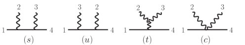
Figure 10: Feynman diagrams for the four-point amplitudes. Absorbing the four-point contact term $(c)$ into diagrams $(s)$, $(t)$, and $(u)$ gives a BCJ representation of the amplitude.

At four points it is straightforward to obtain gauge-theory tree amplitudes that manifest BCJ duality, because all representations of the amplitude in term of diagrams with only cubic vertices have this property BCJ . We, however, also want that, simultaneously, the amplitude satisfies the on-shell Ward identities

$$\mathbb{A}^{\rm tree}_{4}(1^{s},2,3,4^{s})\bigr{|}_{\varepsilon_{2}\rightarrow p_{2}}=0\,,\hskip 42.67912pt\mathbb{A}^{\rm tree}_{4}(1^{s},2,3,4^{s})\bigr{|}_{\varepsilon_{3}\rightarrow p_{3}}=0\,,$$ (5.4)

without using the transversality of the asymptotic state of the remaining gluon,

$$\varepsilon_{3}\cdot p_{3}=0\,,\hskip 42.67912pt\varepsilon_{2}\cdot p_{2}=0\,,$$ (5.5)

respectively. To find such a representation we can start, for example, with Feynman diagrams in Feynman gauge, illustrated in Fig. 10; for four-point trees there is no need for more sophisticated approaches. We then rearrange the diagrams in two ways. First we absorb the four-vertex into the diagrams with only three vertices by matching the color factors and multiplying and dividing by the appropriate propagator. Then we add terms that vanish on shell while demanding that the on-shell Ward identity hold automatically on each gluon leg without using physical state conditions on the other external gluon. The result is an amplitude of the form

$$\mathbb{A}^{\rm tree}_{4}(1^{s},2,3,4^{s})=\frac{n_{s}\,c_{s}}{s-m^{2}}+\frac{n_{t}\,c_{t}}{t}+\frac{n_{u}\,c_{u}}{u-m^{2}}\,,$$ (5.6)

where the Mandelstam invariants are

$$s=(p_{1}+p_{2})^{2}\,,\hskip 28.45274ptt=(p_{2}+p_{3})^{2}\,,\hskip 28.45274ptu=(p_{1}+p_{3})^{2}\,,$$ (5.7)

and $m^{2}=k^{2}_{1}=k^{2}_{4}$ is the mass of the scalar. The color factors are easily read off from the diagrams in Fig. 10,

$$c_{s}=\tilde{f}^{a_{1}a_{2}b}\tilde{f}^{ba_{3}a_{4}}\,,\hskip 28.45274ptc_{t}=\tilde{f}^{a_{2}a_{3}b}\tilde{f}^{ba_{4}a_{1}}\,,\hskip 28.45274ptc_{u}=\tilde{f}^{a_{1}a_{3}b}\tilde{f}^{ba_{2}a_{4}}\,,$$ (5.8)

where the color group structure constants are defined in Eq. (3.9). The color factors satisfy the Jacobi identity

$$c_{t}=c_{s}-c_{u}\,.$$ (5.9)

The $s$-channel kinematic numerator is

$$n_{s}=n(1^{s},2,3,4^{s})=\frac{i}{2}\Bigl{\{}(s-m^{2})\,\varepsilon_{2}\cdot\varepsilon_{3}-2(p_{1}\cdot\varepsilon_{2})\,(p_{12}\cdot\varepsilon_{3})-2(p_{34}\cdot\varepsilon_{2})\,(p_{4}\cdot\varepsilon_{3})\Bigr{\}},$$ (5.10)

with $p_{ij}=p_{i}+p_{j}$. The other two numerators follow from the above: the $u$-channel numerator is obtained by swapping labels $2$ and $3$ in $n_{s}$,

$$n_{u} =n(1^{s},3,2,4^{s}),$$ (5.11)

and the $t$-channel numerator follows from the kinematic Jacobi relation

$$n_{t}=n_{s}-n_{u}\,.$$ (5.12)

The duality between color and kinematics is manifest in Eq. (5.9) and Eq (5.12).

Compared to the result of a Feynman diagram calculation, we have added to the numerators terms proportional to $p_{2}\cdot\varepsilon_{2}$ and $p_{3}\cdot\varepsilon_{3}$ that vanish for asymptotic physical states. While this choice has no physical effect, it greatly simplifies the unitarity construction, especially beyond one loop. Observe that the second term in the projector in Eq. (5.1) replaces one of the polarization vectors with its momentum, which resembles the left-hand side of the on shell Ward identity. The only difference is that the rest of legs may not satisfy physical state conditions, $p_{i}\cdot\varepsilon_{i}=0$, after they have been sewed with other tree amplitudes in the unitarity cut. However, if we can choose the amplitude to satisfy the on-shell Ward identity without demanding physical state conditions, then the Ward identity can be applied term by term in the state sum. So, with the numerators chosen as above, we can simplify the projector to 3PMPRL ; Paolo2PM

$$\sum_{\lambda}\varepsilon^{\mu}(-p)\varepsilon^{\nu}(p)\rightarrow\eta^{\mu\nu}\,,$$ (5.13)

which not only reduces the number of terms, but also eliminates the appearance of the reference momentum and the corresponding spurious propagator. While the propagator numerator (5.13) is analogous to the one in Feynman gauge, there is no need for Fadeev-Popov ghosts or physical-state projectors even when constructing full quantum amplitudes via generalized unitarity. Although the one-loop case in gauge theory is simple enough for the advantage of this reorganization to not be obvious, we will see that, at two loops, the same technique enormously simplifies the $D$ dimensional cut calculations, especially in gravity.

Using the adjusted four-point amplitude, we now construct the one-loop color-dressed gauge-theory cuts. We will then extract their color-ordered components and compare them with the color-ordered four-dimensional cuts. The color-dressed cut in Fig. 7(a) is given by

$${\cal C}_{\rm YM}= \sum_{\rm pols.}\mathbb{A}_{3}^{\rm tree}(3^{s},6,-7^{s})\,\mathbb{A}_{3}^{\rm tree}(7^{s},-5,2^{s})\,\mathbb{A}_{4}^{\rm tree}(1^{s},5,-6,4^{s})$$

$$= \sum_{\rm pols.}\biggl{(}2\tilde{f}^{a_{3}a_{6}a_{7}}\tilde{f}^{a_{7}a_{5}a_{2}}\,(p_{2}\cdot\varepsilon_{-5})\,(p_{3}\cdot\varepsilon_{6})\biggr{)}\times\biggl{(}\frac{c^{\prime}_{t}\,n^{\prime}_{t}}{t}+\frac{c^{\prime}_{s}\,n^{\prime}_{s}}{\tau_{15}}+\frac{c^{\prime}_{u}\,n^{\prime}_{u}}{\tau_{45}}\biggr{)}\,,$$ (5.14)

where the color factors $c^{\prime}_{s,t,u}$ are obtained from Eq. (5.8) by swapping the labels $(2,3)$ into $(5,-6)$ while the kinematic numerator factors $n_{s,t,u}^{\prime}$ are obtained from $n_{s,t,u}$ by the same relabeling. Because the on-shell Ward identities are all automatically satisfied, the state sum simplifies and we only need to replace the product of two polarization vectors by the improved state sum in Eq. (5.13). It is not difficult to simplify the resulting expressions using the cut conditions on the gluon lines, $\tau_{55}=\tau_{66}=0$, and on the matter line, $\tau_{36}=0$.

To compare with the four-dimensional color-ordered cut calculation discussed in Sec. 4 we need to extract the color-ordered components of (5.14). For example, the coefficient of ${\rm Tr}[T^{a_{1}}T^{a_{2}}T^{a_{3}}T^{a_{4}}]$ receives contributions from the numerators $n_{s}^{\prime}$ and $n_{t}^{\prime}$; it is

$$C_{{\rm YM}}^{{\rm(a)}}=\sum_{\rm pols.}\Bigl{(}2(p_{2}\cdot\varepsilon_{-5})\,(p_{3}\cdot\varepsilon_{6})\Bigr{)}\left(\frac{n_{s}^{\prime}}{\tau_{15}}+\frac{n_{t}^{\prime}}{t}\right).$$ (5.15)

Simplifying it using the on shell conditions for the cut lines and the improved gluon physical state projector (5.13), gives

$$C_{\rm YM}^{\rm(a)} =\frac{i}{t\,\tau_{15}}\left(t(s-m_{1}^{2}-m_{2}^{2})^{2}+\tau_{15}(2t\,m_{1}^{2}-2\tau_{15}\,m_{2}^{2}+\tau_{15}t-2st)\right)\,.$$ (5.16)

By relabeling we also obtain the cut in Fig. 7(b)

$$C_{\rm YM}^{\rm(b)} =\frac{i}{t\,\tau_{36}}\left(t(s-m_{1}^{2}-m_{2}^{2})^{2}+\tau_{36}(2t\,m_{2}^{2}-2\tau_{36}\,m_{1}^{2}+\tau_{36}t-2st)\right)\,.$$ (5.17)

Combining the two cuts reproduces the amplitude obtained from four-dimensional cuts in Eq. (4.22).

The match between one-loop integrands obtained from four- and $D$-dimensional methods is not accidental. Discrepancies can arise from two sources: (1) Gram determinants involving five independent vectors, which vanish in four dimensions but not $D$ dimensions and (2) factors of dimension arising from the trace of the metric, $\eta_{\mu}{}^{\mu}=D_{s}$. The former cannot appear, because the one-loop problem contains only four independent momenta. The latter can occur only in bubble diagrams which do not contribute to the classical limit.

The color-dressed cut in Eq. (5.14) immediately gives us the cut with the same topology of the gravity amplitude by replacing each color factor by its corresponding numerator factor, and taking into account the physical state projector that results from the sum over graviton polarizations, which we discuss next.

5.2 Gravity Integrands via BCJ Double Copy

Consider now the gravity generalized cuts in $D=4-2\epsilon$ dimensions. We begin here with the less involved 2PM case as a warm-up for 3PM. Given that the gauge-theory numerators in Eq. (5.10) respect BCJ duality, it is a simple matter to recycle the gauge theory generalized cuts to gravity ones. It is nevertheless important to examine them because, similarly with gauge theory, gravity also exhibits infrared singularities, so it is possible that interference terms between ${\cal O}(\epsilon)$ numerator pieces and $1/\epsilon$ infrared singularities may yield finite terms in addition to those found through a $D=4$ cut calculation. The 2PM scattering amplitude in $D$ dimensions was recently presented in Paolo2PM . Here we discuss a similar analysis of the integrand, focusing on the question of whether any dimensional regularization subtleties can affect the four-dimensional cut construction.

Naively, it would seem that we need the graviton physical-state projector in order to prevent the dilaton and antisymmetric tensor from contributing in double-copy constructions. The $D$-dimensional graviton physical state projector is

$$P^{\mu\nu\rho\sigma}(p,q)=\sum_{\rm pols.}\varepsilon^{\mu\nu}(-p)\varepsilon^{\rho\sigma}(p)= \,\frac{1}{2}\bigl{(}P^{\mu\rho}P^{\nu\sigma}+P^{\mu\sigma}P^{\nu\rho}\bigr{)}-\frac{1}{D_{s}-2}P^{\mu\nu}P^{\rho\sigma}\,,$$ (5.18)

where $P^{\mu\nu}$ is the gluon physical state projector in Eq. (5.1) with momentum $p$ and a null reference momentum $q$. The sum runs over the $D_{s}(D_{s}-3)/2$ physical states of the graviton. As usual we denote any factor $D$ associated with state count as $D_{s}$, so that we may distinguish it from the dimension of the loop integration.

We can simplify the cuts considerably, by using in the double copy construction gluon amplitudes that automatically project out all longitudinal polarizations. In this way the graviton generalized cuts inherit the simplicity of the gluon ones. Indeed, the net effect of using such representations of tree amplitudes is that, in all unitarity cuts, we can replace the physical state projectors with a much simpler one, equivalent to the projector in de Donder gauge,

$$\sum_{\rm pols.}\varepsilon_{\mu\nu}(-p)\varepsilon_{\rho\sigma}(p)=\frac{1}{2}\eta_{\mu\rho}\eta_{\nu\sigma}+\frac{1}{2}\eta_{\nu\rho}\eta_{\mu\sigma}-\frac{1}{D_{s}-2}\eta_{\mu\nu}\eta_{\rho\sigma}\,.$$ (5.19)

We can simplify it even further by observing that the antisymmetric tensor does not couple directly to scalar fields. This implies that, for external scalars, the antisymmetric tensor can appear only in closed loops that do not contain a matter line. Since this violates the rule that every loop needs at least one cut matter line, the antisymmetric tensor cannot, in fact, contribute to the classical potential. We therefore do not need to explicitly symmetrize the projector indices, leaving us with the remarkably simple projector

$$\sum_{\rm pols.}\varepsilon_{\mu\nu}(-p)\varepsilon_{\rho\sigma}(p)=\eta_{\mu\rho}\eta_{\nu\sigma}-\frac{1}{D_{s}-2}\eta_{\mu\nu}\eta_{\rho\sigma}\,.$$ (5.20)

The first term is precisely the one of a naive double copy. The second term is a correction needed to subtract out the dilaton or, alternatively, the trace of the metric fluctuation. Because this projector preserves much of the double copy structure, it is much simpler to use and makes more transparent the transference of gauge-theory properties to gravity. Remarkably, with this reformulation, the propagator for sewing amplitudes is even simpler than the standard de Donder gauge one.

To obtain the gravity cut, we apply the double-copy procedure (3.12) to Eq. (5.14), i.e. we replace the color factors by another copy of the kinematic numerator factors, and find

$${\cal C}_{\rm GR}^{\rm(a)} =\sum_{\rm pols.}\biggl{(}-4(p_{2}\cdot\varepsilon_{-5})^{2}\,(p_{3}\cdot\varepsilon_{6})^{2}\biggr{)}\times i\,\biggl{(}\frac{n^{\prime}_{t}\,n^{\prime}_{t}}{t}+\frac{n^{\prime}_{s}\,n^{\prime}_{s}}{\tau_{15}}+\frac{n^{\prime}_{u}\,n^{\prime}_{u}}{\tau_{45}}\biggr{)}\,.$$ (5.21)

The sum over polarizations generates the simplified physical state projector given in Eq. (5.20).

We have explicitly verified that, when sewing tree amplitudes using the graviton physical-state projectors with $D_{s}=4$, we obtain precisely the result found by summing over four-dimensional helicity states in cuts, given in Eq. (4.34). The reason for this match is the same as in gauge theory: at one loop there is no kinematic object that vanishes in four dimensions but not in $D$ dimensions. The only source of dimensional dependence is then the state-counting parameter $D_{s}$ in the graviton propagator (5.20).

The dependence on $D_{s}$ in the physical state projector does however imply that there is a difference between the $D$-dimensional integrand and the four-dimensional one. For the cut in Fig. 7(a) this difference is

$${\cal C}^{\rm(a)}_{\rm GR}-{\cal C}^{\rm(a)}_{\rm GR}|_{D_{s}=4}= \frac{4m_{1}^{2}m_{2}^{2}(D_{s}-4)}{(D_{s}-2)}\Bigg{[}\frac{t}{\tau_{45}}(2s-2m_{1}^{2}-2m_{2}^{2}-\tau_{15})-\frac{m_{2}^{2}\tau_{15}\tau_{45}}{2m^{2}_{1}t}$$

$$\hskip 28.45274pt\hbox{}\left((s-m_{1}^{2}-m_{2}^{2})^{2}+m_{2}^{2}(m_{1}^{2}\,t-\tau_{15}\tau_{45})\frac{D_{s}}{t(D_{s}-2)}\right)\left(\frac{1}{\tau_{15}}+\frac{1}{\tau_{45}}\right)\Bigg{]}\,.$$ (5.22)

Using $\tau_{15}+\tau_{45}=-t$ on the cut, we can organize the above equation into standard cut integrals. As before, the cut in Fig. 7(b) may be obtained by a simple relabeling. In sec. 12 we will show that this difference between the results of the $D$-dimensional and four-dimensional cut construction has no effect on the classical potential.

6 Integrands at Two Loops

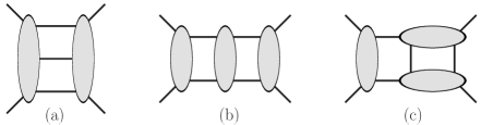
Figure 11: A spanning cuts that determine the full integrand other than quantum bubble on external leg contributions. The complete set of cuts is given including all distinct labels and routing of different particles through the cuts. The lines represent on-shell particles of any type.

In this section we describe the construction of the two-loop gravity integrand using both four-dimensional helicity and $D$-dimensional methods and show explicitly that the four-dimensional construction is sufficient to capture all contributions to the classical potential in four space-time dimensions. As a warm-up, we first analyze the simpler case of color-ordered gauge-theory four-scalar amplitude, pointing out various features of the construction that carry over to the gravity case.

As at one loop, we use the generalized unitarity method hep-ph/9403226 ; hep-ph/9409265 ; hep-ph/9708239 ; hep-th/0412103 ; 0705.1864 , briefly summarized in Sec. 3, to construct the two-loop integrand. The complete quantum integrand can be obtained using a spanning set of cuts, which amounts to the set of cuts from which every term in the loop integrand can be determined. For the two loop massless case such a set is shown in Fig. 11, where all distinct labeling and routings of different particles need to be included. In the massive case there are additional contributions not captured by these cuts, related to bubbles on external legs, but these are purely quantum effects which we ignore.

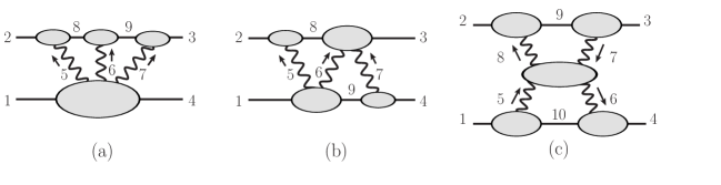
Figure 12: The independent generalized cuts needed at two loops for the classical potential. The remaining contributing cuts are given by simple relabeling of external legs. Here the straight lines represent on-shell scalars and the wiggly lines correspond to on-shell gravitons or gluons.

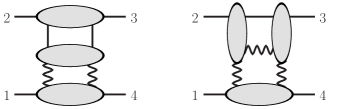
Figure 13: Examples of cuts that are discarded because they have no further classical or iteration contributions to the potential that are not already found in the cuts of Fig. 12.

The set of cuts needed to determine the classical potential is, in fact, a subset of the spanning set. As explained in Sec. 2, the only unitarity cuts that can contain pieces of the classical potential separate the two massive lines on opposite sides of the cut and have one cut matter line in each loop. In addition there are no contributions from diagrams containing a graviton propagator starting and ending on the same scalar line. After dropping from the spanning set all unitarity cuts that do not contain any new contributions that satisfy these criteria, we are left with the cuts in Fig. 12, together with independent ones obtained from relabeling the external lines. The first two cuts, (a) and (b), are just the three-particle cut shown in Fig. 11(a), where the three cut lines are gravitons, but with the additional requirement that one matter line per loop should also be cut. Similarly, the cut in Fig. 12(c) is just the iterated two-particle cut in Fig. 11(b), with all cut lines being gravitons, but with the additional condition imposed that one matter line per loop is cut. Any other cuts, such as the ones shown in Fig. 13, will contain pieces either already determined by the cuts in Fig. 12, or diagrams that do not contribute to the conservative potential. In particular, there are no new classical potential pieces in any iterated two particle cut of the form in Fig. 11(c).

6.1 Warm-up: Gauge-Theory Generalized Cuts in Four Dimensions

Before turning to gravity, we first evaluate the cuts in Fig. 12 for a scalar-coupled gauge theory. Once the gauge-theory cuts have been determined, the gravity ones are obtained easily through double copy.

As in the four-dimensional one loop construction, we take the amplitude to be color ordered so we preserve the cyclic ordering of legs when writing out the tree amplitudes that compose the cut. The first two cuts in Fig. 12 are given by

$$C_{\rm YM}^{\rm(a)} =\!\sum_{h_{5},h_{6},h_{7}=\pm}\!A_{3}^{\rm tree}(3^{s},-7^{-h_{7}},-9^{s})\,A_{3}^{\rm tree}(9^{s},-6^{-h_{6}},-8^{s})\,$$

$$\hskip 99.58464pt\times A_{3}^{\rm tree}(8^{s},-5^{-h_{5}},2^{s})A^{\rm tree}_{5}(1^{s},5^{h_{5}},6^{h_{6}},7^{h_{7}},4^{s})\,,$$ (6.1)

$$C_{\rm YM}^{\rm(b)} =\!\sum_{h_{5},h_{6},h_{7}=\pm}\!A_{4}^{\rm tree}(3^{s},-7^{-h_{7}},-6^{-h_{6}},-8^{s})\,A_{3}^{\rm tree}(8^{s},-5^{-h_{5}},2^{s})$$

$$\hskip 99.58464pt\times A^{\rm tree}_{4}(1^{s},5^{h_{5}},6^{h_{6}},9^{s})\,A_{3}^{\rm tree}(-9^{s},7^{h_{7}},4^{s})\,.$$ (6.2)

The helicity sums run over $2^{3}=8$ possible configurations:

$$\{h_{5},h_{6},h_{7}\}:\,\{+++\},\{---\},\{+--\},\{-++\},\{+-+\},\{-+-\},\{++-\},\{--+\}\,.$$ (6.3)

Similarly, the cut in Fig. 12(c) is,

$$C_{\rm YM}^{\rm(c)}=\sum_{h_{5},h_{6},h_{7},h_{8}=\pm}\!A^{\rm tree}_{3}(3^{s},7^{h_{7}},-9^{s})\,A^{\rm tree}_{3}(9^{s},-8^{-h_{8}},2^{s})\,A^{\rm tree}_{4}(-5^{-h_{5}},8^{h_{8}},-7^{-h_{7}},6^{h_{6}})$$

$$\times A^{\rm tree}_{3}(1^{s},5^{h_{5}},-10^{s})A^{\rm tree}_{3}(10^{s},-6^{-h_{6}},4^{s})\,,$$ (6.4)

where legs $5,6,7,8$ are cut gluon lines and $9$ and $10$ are cut matter lines. The sum over helicity configurations runs over

$$\{h_{5},h_{6},h_{7},h_{8}\}:\,\{++++\},\;\{----\},\;\{+--+\},\;\{++--\},\;\{--++\},\;\{-++-\}\,.$$ (6.5)

The helicity labels correspond to the momentum flow indicated in Fig. 12(c). All other configurations give vanishing contributions, because the four-gluon amplitude represented by the central blob vanishes except for configurations with two legs of positive helicity and two of negative helicity for all outgoing momenta.

As we encountered at one loop, each cut contains both terms that do not appear in any other cut and terms that do. For example, the cut in Fig. 12(a) contains a term in which the lines 1, 4, 5, 6, 7 meet at a single five-point vertex which does not appear in any other cut. It also contains a term corresponding to a two-loop planar double-box graph topology, which also appears in the cut in Fig. 12(b). While we can simplify the cuts following a similar strategy as at one loop, the process of organizing the result in terms of local diagrams and removing such double-counted terms is more complex at two loops. Instead, we will use the simple strategy where the cuts in Eqs. (6.1), (6.2) and (6.4) are directly matched onto the cuts of an ansatz for the integrand with the desired local properties. In this way we simultaneously remove any overcount of terms in cuts and organize the result in terms of Feynman integrals.

To illustrate some important features and to explain the terms that can be dropped when evaluating the cuts in four dimensions, we will summarize the calculation of the cut in Fig. 12(c). In particular, we explain in Sec. 12.2 ambiguities in the integrand when working in four dimensions and why they do not affect the classical potential.

Following similar algebraic steps as at one loop and using standard spinor manipulations we evaluate the terms in the cut in Fig. 12(c) given by the different helicity configurations in Eq. (6.4). We find

$$C_{\rm YM}^{\{++++\}}=-i\frac{m_{1}^{2}m_{2}^{2}\,t}{(-\tau_{58})}\,, C_{\rm YM}^{\{+--+\}}=-i\frac{{\rm tr}^{2}_{-}[728615]}{t^{3}(-\tau_{58})}\,,\quad C_{\rm YM}^{\{+-+-\}}=-i\frac{{\rm tr}^{2}_{-}[827615]}{t^{3}(-\tau_{58})}\,,$$

$$C_{\rm YM}^{\{----\}}=-i\frac{m_{1}^{2}m_{2}^{2}\,t}{(-\tau_{58})}\,, C_{\rm YM}^{\{-++-\}}=-i\frac{{\rm tr}^{2}_{+}[728615]}{t^{3}(-\tau_{58})}\,,\quad C_{\rm YM}^{\{-+-+\}}=-i\frac{{\rm tr}^{2}_{+}[827615]}{t^{3}(-\tau_{58})}\,.$$ (6.6)

While not necessary for the construction of the color-ordered two-loop scalar amplitude with the ordering ${\rm Tr}[T^{a_{1}}T^{a_{2}}T^{a_{3}}T^{a_{4}}]$, to construct the gravity cut corresponding to Fig. 12(c) using the KLT relations we also need the twisted color-ordered cut, obtained by exchanging $\{-5\leftrightarrow 6\}$ in the four-point tree-amplitude factor,

$$C_{\rm YM}^{\prime\rm(c)}=\sum_{h_{5},h_{6},h_{7},h_{8}=\pm}\!A_{3}^{\rm tree}(2^{s},9^{s},-8^{-h_{8}})\,A_{3}^{\rm tree}(7^{h_{7}},-9^{s},3^{s})\,A^{\rm tree}_{4}(6^{h_{6}},8^{h_{8}},-7^{-h_{7}},-5^{h_{5}})$$

$$\times A^{\rm tree}_{3}(1^{s},5^{h_{5}},-10^{s})A^{\rm tree}_{3}(10^{s},-6^{-h_{6}},4^{s})\,.$$ (6.7)

The sum runs over the helicity configurations in Eq. (6.5). Using the BCJ amplitudes relation in Eq. (4.24),

$$A^{\rm tree}_{4}(6^{h_{6}},8^{h_{8}},-7^{-h_{7}},-5^{h_{5}})=-\frac{\tau_{58}}{\tau_{68}}A^{\rm tree}_{4}(-5^{h_{5}},8^{h_{8}},-7^{-h_{7}},6^{h_{6}})\,,$$ (6.8)

it is not difficult to find that the twisted cut and its helicity-labeled components are simply

$$C_{\rm YM}^{\prime\{h_{5},h_{6},h_{7},h_{8}\}}=\frac{(-\tau_{58})}{\tau_{68}}C_{\rm YM}^{\{h_{5},h_{6},h_{7},h_{8}\}}\,,\hskip 28.45274ptC_{\rm YM}^{\prime\rm(c)}=\frac{(-\tau_{58})}{\tau_{68}}C_{\rm YM}^{\rm(c)}\,.$$ (6.9)

The rational factor effectively replaces the $-1/\tau_{58}$ propagator with the $1/\tau_{68}$ one, corresponding to the relabeled four-point amplitude in the middle blob in Fig. 12(c).

Next, we evaluate the two remaining traces in Eq. (6.6). We split them into parity-even and parity-odd parts, as at one-loop, resulting in

$${\rm tr}_{\pm}^{2}[827615] ={\cal E}_{1}^{2}+{\cal O}_{1}^{2}\pm 2{\cal O}_{1}{\cal E}_{1}\,,$$ (6.10)

$${\rm tr}_{\pm}^{2}[728615] ={\cal E}_{2}^{2}+{\cal O}_{2}^{2}\pm 2{\cal O}_{2}{\cal E}_{2}\,.$$ (6.11)

It is however clear that, in the complete cut, the parity-odd part cancels out, so we only need to compute ${\cal O}_{i}^{2}$. Evaluating the trace using standard gamma-matrix identities we find

$${\cal E}_{1}^{2} =\frac{1}{4}t^{2}\bigl{(}\tau_{12}\tau_{58}-\tau_{18}\tau_{25}\bigr{)}^{2}\,,\qquad{\cal O}_{1}^{2}={\cal E}_{1}^{2}-\tau_{58}^{2}m_{1}^{2}m_{2}^{2}\,t^{2}\,.$$ (6.12)

$${\cal E}_{2}^{2} =\frac{1}{4}t^{2}\bigl{(}\tau_{24}\tau_{57}+\tau_{17}\tau_{57}\bigr{)}^{2}\,,\qquad{\cal O}_{2}^{2}={\cal E}_{2}^{2}-\tau_{57}^{2}m_{1}^{2}m_{2}^{2}\,t^{2}\,,$$ (6.13)

where $t=(p_{2}+p_{3})^{2}$ and $\tau_{ij}=2p_{i}\cdot\ell_{j}$.

Adding up the contributions of the six helicity configurations, we find that the complete four-dimensional cut in Fig. 12(c) is given by

$$C_{\rm YM}^{\rm(c)} =-2i\frac{1}{(-\tau_{58})}\biggl{[}m_{1}^{2}m_{2}^{2}t+\frac{1}{t^{3}}\bigl{(}{\cal E}_{1}^{2}+{\cal O}_{1}^{2}+{\cal E}_{2}^{2}+{\cal O}_{2}^{2}\bigr{)}\biggr{]}$$ (6.14)

$$=-2i\frac{1}{(-\tau_{58})}\biggl{[}m_{1}^{2}m_{2}^{2}t+\frac{1}{2t}\bigl{(}(\tau_{12}\tau_{58}-\tau_{18}\tau_{25})^{2}-2\tau_{58}^{2}m_{1}^{2}m_{2}^{2}+(\tau_{24}\tau_{57}+\tau_{17}\tau_{57})^{2}-2\tau_{57}^{2}m_{1}^{2}m_{2}^{2}\bigr{)}\biggr{]}\,.$$

The twisted cut is simply obtained through Eq. (6.9).

If naively continued outside of four dimensions, the expression (6.14) contains a spurious singularity. To expose this issue we construct the maximal cut obtained by imposing the additional cut condition

$$\tau_{58}=0\,.$$ (6.15)

Together with the initial six cut conditions, this corresponds to cutting the maximum number of propagators for a four-point two-loop amplitude; consequently, the result should be local, as can be checked by solving the seven cut conditions in four dimensions. However, with this additional cut condition, we get the maximal cut interpreted as a $D$-dimensional expression

$$C_{\rm YM}^{\rm maxcut}=-\frac{1}{t}\,\tau_{18}^{2}\,\tau_{25}^{2}\,.$$ (6.16)

It contains a $1/t$ pole. Maximal cuts should be local, since they are nothing more than sums of products of three vertices. This strongly suggests that the correct $D$-dimensional expression is missing a term proportional to a Gram determinant that vanishes in four dimensions but not in $D$ dimensions.

This is indeed the case. To remove the spurious $1/t$ singularity we add a term proportional to the Gram determinant

$$G_{5}=16\det\left(\begin{matrix}p_{1}\cdot p_{1}&p_{1}\cdot p_{2}&p_{1}\cdot p_{3}&p_{1}\cdot\ell_{5}&p_{1}\cdot\ell_{8}\\ p_{2}\cdot p_{1}&p_{2}\cdot p_{2}&p_{2}\cdot p_{3}&p_{2}\cdot\ell_{5}&p_{2}\cdot\ell_{8}\\ p_{3}\cdot p_{1}&p_{3}\cdot p_{2}&p_{3}\cdot p_{3}&p_{3}\cdot\ell_{5}&p_{3}\cdot\ell_{8}\\ \ell_{5}\cdot p_{1}&\ell_{5}\cdot p_{2}&\ell_{5}\cdot p_{3}&\ell_{5}\cdot\ell_{5}&\ell_{5}\cdot\ell_{8}\\ \ell_{8}\cdot p_{1}&\ell_{8}\cdot p_{2}&\ell_{8}\cdot p_{3}&\ell_{8}\cdot\ell_{5}&\ell_{8}\cdot\ell_{8}\end{matrix}\right),$$ (6.17)

which vanishes in four dimensions. By adjusting the coefficient of $G_{5}$ we can remove the spurious singularity. This results in a cut that is now valid in $D$-dimensions,

$$C_{\rm YM}=-2i\frac{1}{(-\tau_{58})}\biggl{[}m_{1}^{2}m_{2}^{2}t+\frac{1}{t^{3}}\Bigl{(}{\cal E}_{1}^{2}+{\cal O}_{1}^{2}+{\cal E}_{2}^{2}+{\cal O}_{2}^{2}-t\,G_{5}\Bigr{)}\biggr{]}\,,$$ (6.18)

where the state-counting parameter is $D_{s}=4$. An alternative way to arrive at the same result is to match an ansatz written in terms of local diagrams (which by definition have no spurious singularities) onto $C_{\text{YM}}^{(c)}$. The twisted cut can be obtained from Eq. (6.18) via Eq. (6.9).

6.2 Gravity Generalized Cuts in Four Dimensions

The KLT relations (3.5) provide a simple path for assembling the gauge-theory cut components constructed above into analytic expression for the three gravity cuts in Fig. 12. Those corresponding to Fig. 12(a,b) are

$$C_{\rm GR}^{\rm(a)} =\sum_{h_{5},h_{6},h_{7}=\pm}\!M_{3}^{\rm tree}(2^{s},8^{s},-5^{-h_{5}})\,M_{3}^{\rm tree}(-6^{-h_{6}},-8^{s},9^{s})$$

$$\hskip 85.35826pt\hbox{}\times M_{3}^{\rm tree}(7^{h_{7}},-9^{s},3^{s})\,M_{5}^{\rm tree}(1^{s},5^{h_{5}},6^{h_{6}},7^{h_{7}},4^{s})\,,$$ (6.19)

$$C_{\rm GR}^{\rm(b)} =\sum_{h_{5},h_{6},h_{7}=\pm}\!M_{3}^{\rm tree}(2^{s},8^{s},-5^{-h_{5}})\,M_{4}^{\rm tree}(-7^{-h_{7}},-6^{-h_{6}},-8^{s},3^{s})$$

$$\hskip 85.35826pt\hbox{}\times M^{\rm tree}_{4}(1^{s},5^{h_{5}},6^{h_{6}},9^{s})\,M_{3}^{\rm tree}(-9^{s},7^{h_{7}},4^{s})\,,$$ (6.20)

where the helicity configurations run over the eight possibilities in Eq. (6.3), except that here the $\pm$ refer to the spin states of gravitons instead of those of gluons. The gravity tree amplitudes can be simply evaluated using the KLT relations (3.5). Similarly, the remaining cut in Fig. 12(c) is

$$C_{\rm GR}^{\rm(c)} =\sum_{h_{5},h_{6},h_{7},h_{8}=\pm}\!M^{\rm tree}_{3}(2^{s},9^{s},-8^{-h_{8}})\,M^{\rm tree}_{3}(7^{h_{7}},-9^{s},3^{s})\,M^{\rm tree}_{4}(-5^{-h_{5}},6^{h_{6}},-7^{-h_{7}},8^{h_{8}})$$

$$\hbox{}\hskip 113.81102pt\times M^{\rm tree}_{3}(1^{s},5^{h_{5}},-10^{s})M^{\rm tree}_{3}(10^{s},-6^{-h_{6}},4^{s})$$

$$=-it\sum_{h_{5},h_{6},h_{7},h_{8}=\pm}\biggl{[}A^{\rm tree}_{3}(2^{s},9^{s},-8^{-h_{8}})\,A^{\rm tree}_{3}(7^{h_{7}},-9^{s},3^{s})\,A^{\rm tree}_{4}(-5^{-h_{5}},6^{h_{6}},-7^{-h_{7}},8^{h_{8}})$$

$$\hbox{}\hskip 113.81102pt\times A^{\rm tree}_{3}(1^{s},5^{h_{5}},-10^{s})\,A^{\rm tree}_{3}(10^{s},-6^{-h_{6}},4^{s})\biggr{]}$$

$$\hskip 78.24507pt\hbox{}\times\biggl{[}A^{\rm tree}_{3}(2^{s},9^{s},-8^{-h_{8}})\,A^{\rm tree}_{3}(7^{h_{7}},-9^{s},3^{s})\,A^{\rm tree}_{4}(6^{h_{6}},8^{h_{8}},-7^{-h_{7}},-5^{h_{5}})$$

$$\hbox{}\hskip 113.81102pt\times A^{\rm tree}_{3}(1^{s},5^{h_{5}},-10^{s})\,A^{\rm tree}_{3}(10^{s},-6^{-h_{6}},4^{s})\biggr{]}\,,$$ (6.21)

where legs $5,6,7,8$ are cut graviton lines and $9$ and $10$ are cut matter lines. As for the gluon case, some helicity configurations have vanishing contributions because of the properties of the four-graviton amplitude factor, so the sum over helicities in Eq. (6.21) effectively runs over the configurations in Eq. (6.5). As at one loop, we project out the dilaton and axion simply by requiring that the helicities of gluons in the two gauge-theory factors in Eqs. (6.19), (6.20) and (6.21) be identical.

Upon using the gauge-theory tree amplitudes given in Appendix B we find compact expressions for the three types of cuts in Fig. 12, which can subsequently be assembled into a single integrand, as we discuss below. It is instructive to inspect in some detail the cut in Fig. 12(c), in order to understand potential issues with carrying out the calculation in four dimensions compared to $D$ dimensions. In general, we prefer the four-dimensional expressions because their complexity at higher loops increases slower than that of their $D$-dimensional counterparts.

The cut components, labeled by the helicities of the cut graviton lines in Fig. 12(c) are obtained through the KLT relations in terms of the direct and twisted YM cut components in Eqs. (6.6) and (6.7)

$$C_{\rm GR}^{\{h_{1}h_{2}h_{3}h_{4}\}} =-i\,t\,C_{\rm YM}^{\{h_{1}h_{2}h_{3}h_{4}\}}C_{\rm YM}^{\prime\{h_{1}h_{2}h_{3}h_{4}\}}\,.$$ (6.22)

As explained above, by identifying the helicity labels in the two gauge-theory amplitudes we project out the dilaton and axion contributions to cuts. Using the relation in Eq. (6.9), we can read off the results in different helicity configurations as

$$C_{\rm GR}^{\{++++\}}=i\frac{m_{1}^{4}m_{2}^{4}t^{3}}{(-\tau_{58})\tau_{68}}\,, C_{\rm GR}^{\{+--+\}}=i\frac{{\rm tr}^{4}_{-}[728615]}{t^{5}(-\tau_{58})\tau_{68}}\,,\quad\; C_{\rm GR}^{\{+-+-\}}=i\frac{{\rm tr}^{4}_{-}[827615]}{t^{5}(-\tau_{58})\tau_{68}}\,,$$

$$C_{\rm GR}^{\{----\}}=i\frac{m_{1}^{4}m_{2}^{4}t^{3}}{(-\tau_{58})\tau_{68}}\,, C_{\rm GR}^{\{-++-\}}=i\frac{{\rm tr}^{4}_{+}[728615]}{t^{5}(-\tau_{58})\tau_{68}}\,,\quad\; C_{\rm GR}^{\{-+-+\}}=i\frac{{\rm tr}^{4}_{+}[827615]}{t^{5}(-\tau_{58})\tau_{68}}\,.$$ (6.23)

Summing over all helicity configurations of gravitons crossing the iterated two-particle cuts, we find

$$C_{\rm GR}^{\rm(c)} =-i\biggl{[}2t^{2}m_{1}^{4}m_{2}^{4}+\frac{1}{t^{6}}\Bigl{(}{\rm tr}^{4}_{-}[728615]+{\rm tr}^{4}_{-}[827615]+{\rm tr}^{4}_{+}[728615]+{\rm tr}^{4}_{+}[827615]\Bigr{)}\biggr{]}$$

$$\quad\times\biggl{[}\frac{1}{(-\tau_{58})}+\frac{1}{\tau_{68}}\biggl{]}\,,$$ (6.24)

where we used the partial fractioning identity (recall that momenta are flowing as indicated in Fig. 12(c))

$$\frac{1}{(-\tau_{58})\tau_{68}} =-\frac{1}{t}\biggl{[}\frac{1}{(-\tau_{58})}+\frac{1}{\tau_{68}}\biggl{]}\,.$$ (6.25)

By inspecting Eq. (6.24) it is easy to see that all parity-odd terms cancel out. We can evaluate the traces using Eqs. (6.10) and (6.11)

$$C_{\rm GR}^{\rm(c)} =-2i\biggl{[}t^{2}m_{1}^{4}m_{2}^{4}+\frac{1}{t^{6}}\Bigl{(}{\cal E}_{1}^{4}+{\cal O}_{1}^{4}+6{\cal O}_{1}^{2}{\cal E}_{1}^{2}+{\cal E}_{2}^{4}+{\cal O}_{2}^{4}+6{\cal O}_{2}^{2}{\cal E}_{2}^{2}\Bigr{)}\biggr{]}\biggl{[}\frac{1}{(-\tau_{58})}+\frac{1}{\tau_{68}}\biggl{]}\,,$$ (6.26)

where the even-squared and odd-squared terms are given in Eqs.  (6.12) and (6.13).

As for the YM cut with the same topology, if we naively extend Eq. (6.26) to $D$ dimensions we encounter a spurious singularity in the maximal cut, which we can remove by adding in Eq. (6.17) a term proportional to the Gram determinant, that vanishes in four dimensions. Doing so gives,

$$C_{\rm GR}^{\rm(c)} =-2i\biggl{[}t^{2}m_{1}^{4}m_{2}^{4}+\frac{1}{t^{6}}\Bigl{(}{\cal E}_{1}^{4}+{\cal O}_{1}^{4}+6{\cal O}_{1}^{2}{\cal E}_{1}^{2}+{\cal E}_{2}^{4}+{\cal O}_{2}^{4}+6{\cal O}_{2}^{2}{\cal E}_{2}^{2}$$

$$\qquad\qquad-2tG_{5}({\cal E}_{1}^{2}+{\cal O}_{1}^{2}+{\cal E}_{2}^{2}+{\cal O}_{2}^{2})+t^{2}G_{5}^{2}\Bigr{)}\biggr{]}\biggl{[}\frac{1}{(-\tau_{58})}+\frac{1}{\tau_{68}}\biggl{]}\,.$$ (6.27)

As we will see, further terms that vanish in four dimensions (and therefore proportional to $G_{5}$) are necessary to obtain the complete $D$-dimensional cut. Nevertheless, all terms proportional to $G_{5}$ do not contribute to the classical potential, as we discuss in Sec. 12.2.

For comparison, the cut in Fig. 12(c) for the scattering of scalars coupled to a graviton, dilaton and antisymmetric tensor (or axion) is given by the simple double copy:

$$C_{\rm GR}^{\rm(c)}+C_{\rm\phi a}^{\rm(c)} =-4i\biggl{[}tm_{1}^{2}m_{2}^{2}+\frac{1}{t^{3}}\Bigl{(}{\cal E}_{1}^{2}+{\cal O}_{1}^{2}+{\cal E}_{2}^{2}+{\cal O}_{2}^{2}-tG_{5}\Bigr{)}\biggr{]}^{2}\biggl{[}\frac{1}{(-\tau_{58})}+\frac{1}{\tau_{68}}\biggl{]}\,.$$ (6.28)

This expression holds for kinematics in general dimension, but with $D_{s}=4$.

6.3 $D$-Dimensional Generalized Cuts

The evaluation of the $D$-dimensional version of the generalized cuts in Fig. 12 is similar to the evaluation of the one-loop $D$-dimensional cuts in Sec. 4, except that the relevant gauge-theory trees are somewhat more complicated. Besides the two-scalar three-gluon tree-level amplitude needed for the cut in Fig. 12(a), we also need the four-gluon amplitude in a BCJ form that also satisfies the on-shell Ward identity Eq. (B.13) without use of transversality of the external states. These tree amplitudes are given in Appendix B. By using a good basis choice and BCJ duality, the amplitudes are determined by specifying a single numerator. Because BCJ duality is manifest, the desired gravity cuts follow immediately from the gauge-theory ones through the double-copy substitution in Eq. (3.12).

As at one-loop, we exploit the compact physical-state projector in Eq. (5.20), which is a consequence of the on-shell Ward identities holding without imposing the transversality of gluon and graviton asymptotic states and of the decoupling of antisymmetric tensor. This trick simplifies the two-loop calculation enormously. We will not include the details since the calculations are straightforward extensions of the one-loop ones. We will however comment on the result for the cut in Fig. 12(c) and compare it with the four-dimensional expression in Eq. (6.26).

Taking $D_{s}=\eta_{\mu}^{\ \mu}=4$, the cut in Fig. 12(c) evaluates to the rather compact expression

$$C_{\rm GR}^{\rm(c)}= -2i\biggl{[}t^{2}m_{1}^{4}m_{2}^{4}+\frac{1}{t^{6}}\Bigl{(}{\cal E}_{1}^{4}+{\cal O}_{1}^{4}+6{\cal O}_{1}^{2}{\cal E}_{1}^{2}+{\cal E}_{2}^{4}+{\cal O}_{2}^{4}$$

$$\qquad\qquad+6{\cal O}_{2}^{2}{\cal E}_{2}^{2}-2tG_{5}({\cal E}_{1}^{2}+{\cal O}_{1}^{2}+{\cal E}_{2}^{2}+{\cal O}_{2}^{2})+t^{2}G_{5}^{2}\Bigr{)}$$

$$\qquad\qquad-\frac{1}{t}(2m_{1}^{2}m_{2}^{2}+(\tau_{12}-\tau_{18}+\tau_{25}-\tau_{58})^{2})G_{5}\biggr{]}\biggl{(}\frac{1}{(-\tau_{58})}+\frac{1}{\tau_{68}}\biggl{)}\,,$$ (6.29)

where $G_{5}$ is the Gram determinant in Eq. (6.17). We note that, apart from the $G_{5}$ terms we found by requiring absence of a spurious pole in the maximal cut of the naive $D$-dimensional continuation of the four-dimensional result in Eq. (6.27), the complete $D$-dimensional calculation yields additional terms linear in $G_{5}$. The other cuts are also straightforward to evaluate, although we have not obtained compact $D$-dimensional expressions for them.

6.4 Merging the Cuts into an Integrand

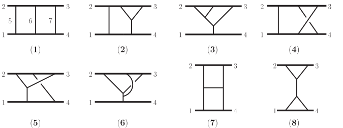
Figure 14: The eight independent diagrams with only cubic vertices showing the propagator structure of integrals which contribute to the classical potential. The thick lines correspond to massive particles. All other diagrams are given by relabeling the external legs. In the main text, we will denote each diagram using bold label, e.g. diagram $\bm{1}$ for the first diagram.

Once the cuts have been evaluated, the next step is to reorganize them into an integrand. We do this for both their four and $D$-dimensional versions. While obtaining the integrand from the four-dimensional cuts turns out to be sufficient, it is nevertheless important to verify that no subtleties arise from truncating the integrand to four dimensions, given the fact that the integrated amplitude is infrared divergent.

In general, different unitarity cuts contain information about the same terms in the integrand. For example, contributions to diagram $\bm{1}$ in Fig. 14 are found in both cuts (a) and (b) of Fig. 12 while contributions to diagram $\bm{7}$ in Fig. 14 appear both in cuts (b) and (c) of Fig. 12. Such double counting can be removed either during the construction of the integrand  BDDPR ; TwoLoopSplitting or after integration Bern:2002tk . We will choose the former approach, as it meshes well with our integration methods described in the next sections.

To determine the numerators for the diagrams in Fig. 14 we construct an ansatz for each of them. While contact diagrams with four- or higher-point vertices can be included in the ansatz, we choose to minimize the number of independent graphs by instead using diagrams that have only cubic vertices as shown in Fig. 14, and capturing contact terms by multiplying and dividing by appropriate propagators. The highest number of loop-momentum factors in each term of the ansatz follows from the two-derivative nature of gravity couplings, counting two such factors for each three-point vertex. As we will see, it is not necessary to saturate the maximal power counting for all diagrams. After including relabelings of external lines, the eight diagram topologies shown in Fig. 14 are the minimal set needed for matching the three unitarity cuts in Fig. 12. We impose the natural requirement that the symmetries of a diagram are also symmetries of its numerator factor. The parameters of the ansatze are then fixed by computing their generalized cuts (including contributions from the relabelings) and match to those in Fig. 12 computed earlier via multiplying tree amplitudes. Once this is done, the merged integrand simultaneously satisfies all other generalized unitarity cuts related to Fig. 12 by exchanging the external legs, because the relabeling is built-in explicitly.

An observation that leads to simplifications when imposing diagram symmetries is that on-shell conditions may be imposed on a given leg in a given diagram if that leg is on shell in all cuts that contribute to that diagram. For example, the on-shell conditions for the three gravitons can be applied to the numerator of diagram $\bm{1}$ because these gravitons are on shell in both cuts (a) and (b) in Fig. 12. The four gravitons that connect to matter lines in diagram $\bm{7}$ must however be treated off shell because they are off shell in cut (b) in Fig. 12. On the other hand, we can use the on shell condition for the two matter lines in diagrams $\bm{7}$ and $\bm{8}$ without affecting the classical potential because only cuts (b) and (c) in Fig. 12 source them and they both place the matter lines on shell.

In the construction of the ansatz for each diagram’s numerator, we only require a sufficiently high power of loop momenta such that a solution exists and matches either to four-dimensional cuts or to $D$-dimensional cuts. For example, diagram $\bm{1}$ in Fig. 14 does not require any powers of loop momenta in the numerators, while the numerator of diagram $\bm{6}$ requires the maximum of 12 powers of loop momenta to match the cuts, prior to dropping quantum terms containing more than 4 powers of loop momenta in the numerator.

In general, the numerators contain free parameters because of the possibility of assigning the same contact term to different diagrams without changing the value of integrand. We choose the remaining undetermined parameters to simplify the matching with the effective field theory amplitudes in Sec. 10. For example, we chose diagram (1) to have a numerator proportional to the third power of the numerator in tree-level four-scalar amplitude, i.e.

$$N^{(1)}_{\rm GR}(1,2,3,4)=\left((s-m_{1}^{2}-m_{2}^{2})^{2}-\frac{4}{D_{s}-2}m_{1}^{2}m_{2}^{2}\right)^{3}\,.$$ (6.30)

By imposing diagram’s symmetry on all numerators, simple relabeling gives us the value of the numerators with swapped legs. For example, the numerator corresponding to the case where legs 1 and 4 are swapped is simply,

$$N^{(1)}_{\rm GR}(1,3,2,4)=\left((u-m_{1}^{2}-m_{2}^{2})^{2}-\frac{4}{D_{s}-2}m_{1}^{2}m_{2}^{2}\right)^{3}\,.$$ (6.31)

The numerators of the other diagrams are more involved. The free parameters also provide a nontrivial check since they should cancel out in the final integrated amplitude. We have performed extensive checks to confirm this property.

Graph	External relabeling
1	(1 2 3 4),  (1 3 2 4)
2	(1 2 3 4),  (1 3 2 4),  (4 3 2 1),  (4 2 3 1),  $+\{1,4\}\leftrightarrow\{2,3\}$
3	(1 2 3 4),  (1 3 2 4),  $+\{1,4\}\leftrightarrow\{2,3\}$
4	(1 2 3 4),  (1 3 2 4),  (4 3 2 1),  (4 2 3 1)
5	(1 2 3 4),  (4 2 3 1),  $+\{1,4\}\leftrightarrow\{2,3\}$
6	(1 2 3 4),  $+\{1,4\}\leftrightarrow\{2,3\}$
7	(1 2 3 4),  (1 3 2 4)
8	(1 2 3 4)

Table 1: List of 27 cubic diagrams from relabeling of the eight graphs in Fig. 14. The right column gives all independent labels by exchanging the original external legs $(1234)$ in each graph in Fig. 14. Here $\{1,4\}\leftrightarrow\{2,3\}$ means swapping $1,4$ with $2,3$ in all the previous labels. For example, this yields (2 1 4 3) and (2 4 1 3) for graph 5.

Once a valid set of numerators with the properties described above has been determined, we can treat the diagrams as if they were ordinary off-shell Feynman diagrams. In particular, the diagram numerators are functions of the external labels and can be taken as respecting diagram symmetry. While on-shell conditions have been used in their construction, we can view their use as merely affecting terms with no contributions to the classical potential.

We write the part of the two-loop four-scalar amplitude necessary for the extraction of the complete 3PM conservative potential as a sum over 27 diagrams,

$$M^{\rm 2\hbox{-}loop}=(4E_{1}E_{2})\,i\mathcal{M}_{3}=i(8\pi G)^{3}\int\frac{d^{D}\ell_{5}}{(2\pi)^{D}}\frac{d^{D}\ell_{6}}{(2\pi)^{D}}\sum_{i=1}^{27}{\cal I}^{(i)}\,,$$ (6.32)

where $\mathcal{M}_{3}$ is the 3PM amplitude including a nonrelativistic normalization $1/4E_{1}E_{2}$. We will use this normalization for the amplitudes $\mathcal{M}_{n}$ presented in Sec. 9 and Sec. 10. The sum runs over 27 distinct diagrams arising from the independent relabelings of the external legs of the eight diagrams in Fig. 14, which are taken to correspond to $i=1,\dots,8$ and are found in the ancillary Mathematica text file Integrand_TwoLoop.m AttachedFile . The relabelings are listed in Table 1. The integrands are expressed in terms of numerators and denominators, in the usual way:

$${\cal I}^{{i}}=\frac{N^{(i)}}{D^{(i)}}\,.$$ (6.33)

The denominators are simply the Feynman propagators of the corresponding diagram. For example, for diagram (1) of Fig. 14,

$$D^{(1)}=\ell_{5}^{2}\ell_{6}^{2}(\ell_{5}+\ell_{6}-p_{2}-p_{3})^{2}(\ell_{5}-p_{2})^{2}(\ell_{5}+\ell_{6}-p_{2})^{2}(\ell_{5}+p_{1})^{2}(\ell_{5}+\ell_{6}+p_{1})^{2}\,,$$ (6.34)

where we have suppressed the standard Feynman $i\epsilon$ prescription, which should be included for each propagator. The numerators in this file are valid in $D$ dimensions, but with the state-counting parameter $D_{s}=4$ for simplicity.

We have also constructed several alternative integrands starting both from cuts constructed in four and $D$ dimensions, as described above. As already noted, expressions obtained with these two starting points differ by terms proportional to the Gram determinant $G_{5}$ in Eq. (6.17), which vanishes in four dimensions. In addition, when we use helicity methods, the state-counting parameter is automatically taken to be $D_{s}=4$. We have explicitly checked that integrands extracted from four dimensions and $D$ dimensions and using $D_{s}=4$ or $D_{s}=4-2\epsilon$ lead to identical final results for the potential.

The independence of the potential on the details of the dimensional regularization prescription is not accidental. In Sec. 12.2, we explain why any two-loop integral containing a Gram determinant that vanishes in four dimensions cannot contribute to the classical potential and why the results are independent of the choice of prescription for the $D_{s}$ parameter. The net effect is that, analogous to the way as it works at one loop, the difference between constructing the integrand in four and in $D$ dimensions does not affect the classical potential. This, of course, agrees with naive expectations.

7 Nonrelativistic Integration

In the previous sections we constructed fully relativistic expressions for the integrands relevant to classical potential scattering. It would then seem natural to integrate these objects using fully relativistic methods. While such a strategy is straightforward and efficient at one loop, see e.g. Sec. 12.1, it becomes considerably more difficult at two-loop order. Indeed from the point of view of scalability to high loop orders, the situation is even more dire. To match the current state of the art in the PN expansion requires computational power at 5PN order, corresponding to full integration at five loops 1902.10571 ; 1902.11180 . This is a tall order, already extending far beyond the capabilities of any known fully relativistic loop integration method.

Clearly, a simpler method of integration must exist. After all, conventional methods using equations of motion or NRGR have already achieved results up to 5PN, and these calculations certainly did not necessitate the evaluation of difficult relativistic integrals. The simple fact that these existing formalisms are by construction nonrelativistic and classical suggests an alternative path to integration.

In this section, we describe such a method, which we dub “nonrelativistic integration”. This approach is by design as similar as possible to the method of integration which appears in NRGR NRGR . Roughly speaking, it involves performing all energy integrations first, and then integrating spatial $(D-1)$-momenta.

We begin with a brief summary of the complete procedure. We then go through the details carefully by working through several explicit examples at one and two loops.

7.1 General Procedure

Our integration procedure is constructed to extend mechanically to arbitrary loop orders. In this section we outline the core strategy of this method, which has been tested explicitly at one and two loops. We believe that this basic approach should apply beyond this order, though as past experience suggests, subtleties may arise due to new topologies and certain physical phenomena which only appear at higher orders, e.g. the tail effect TailEffect1 ; TailEffect2 ; TailEffect3 ; TailEffect4 ; TailEffect5 ; TailEffect6 . See Sec. 12.3 for further comments.

Consider a general multi-loop integral characterizing the scattering of matter fields through graviton exchange:

$$I=\bigg{[}\prod_{i=1}^{n_{L}}\int\frac{d^{D-1}\bm{\ell}_{i}}{(2\pi)^{D-1}}\bigg{]}\bigg{[}\prod_{i=1}^{n_{L}}\int\frac{d\omega_{i}}{2\pi}\bigg{]}\,{\cal I}=\bigg{[}\prod_{i=1}^{n_{L}}\int\frac{d^{D-1}\bm{\ell}_{i}}{(2\pi)^{D-1}}\bigg{]}\,\widetilde{\cal I},$$ (7.1)

where $i$ runs over $n_{L}$ loop momenta $\ell_{i}=(\omega_{i},\bm{\ell}_{i})$ and we have split the integration over the energy and $(D-1)$-momentum components. For convenience, we will typically choose the $\ell_{i}$ to be a subset of the momenta flowing through internal graviton lines. We follow the standard dimensional regularization prescription for the spatial directions only.

We pause to define notation which will be employed for the rest of the paper. From here on, the script quantity ${\cal I}$ will denote a full relativistic integrand, e.g. as computed earlier in Sec. 6. The integrand ${\cal I}$ is a function of $n_{L}$ loop energies and $n_{L}$ loop $(D-1)$-momenta, and will appear below with subscripts labeling the particular diagram. Meanwhile, the tilded script quantity $\widetilde{\cal I}=\prod_{i=1}^{n_{L}}\int\frac{d\omega_{i}}{2\pi}\,{\cal I}$ will denote a spatial integrand, which is defined to be the energy integral of a corresponding full relativistic integrand. The spatial integrand is a function of $n_{L}$ loop $(D-1)$-momenta. Throughout, the spatial integration will appear with subscripts labeling the corresponding diagram.

The process of integration has three key steps which we now discuss broadly. The detailed mechanics will be illustrated with one-loop examples in Sec. 7.2 and two-loop examples in Sec. 7.3.

Step 1: Determine the Effective Numerator

The integrand takes the general form

$${\cal I} =\bigg{[}\prod_{i=1}^{n_{M}}\frac{1}{\varepsilon_{i}^{2}-\bm{k}_{i}^{2}-m_{i}^{2}}\bigg{]}\bigg{[}\prod_{j=1}^{n_{G}}\frac{1}{\omega_{j}^{2}-\bm{\ell}_{j}^{2}}\bigg{]}\,{\cal N}\,,$$ (7.2)

where $i$ runs over $n_{M}$ internal scalar field lines whose energy, $(D-1)$-momentum, and mass are $\varepsilon_{i}$, $\bm{k}_{i}$, and $m_{i}$, and $j$ runs over $n_{G}$ internal graviton lines whose energy and $(D-1)$-momentum are $\omega_{j}$ and $\bm{\ell}_{j}$. Of course, these energies and $(D-1)$-momenta are not independent. All kinematic parameters depend implicitly on the external masses $m_{1}$ and $m_{2}$, external $(D-1)$-momenta $\bm{p}$ and $\bm{p}^{\prime}$, as well as $n_{L}$ independent loop energies and $(D-1)$-momenta.

We can factorize the scalar propagators into matter and antimatter poles,

$$\frac{1}{\varepsilon_{i}^{2}-\bm{k}_{i}^{2}-m_{i}^{2}} =\frac{1}{\varepsilon_{i}-\sqrt{\bm{k}_{i}^{2}+m_{i}^{2}}}\,\frac{1}{\varepsilon_{i}+\sqrt{\bm{k}_{i}^{2}+m_{i}^{2}}}\,.$$ (7.3)

The matter poles occur at positive energy values and correspond to singularities which can genuinely appear in the low-energy scattering of interest. On the other hand, the antimatter poles occur at negative energy values. These states are never on shell in the nonrelativistic regime and correspond to high-energy modes. Note that even though the antimatter poles never become singular for low energy kinematics, they still have an effect since these factors should still be expanded in the nonrelativistic limit, yielding classical velocity corrections.

Next, we combine all contributions from the original numerator, the force-carrier (graviton) propagators, and the antimatter poles into an “effective numerator”,

$$\widetilde{\cal N}=\bigg{[}\prod_{i=1}^{n_{M}}\frac{1}{\varepsilon_{i}+\sqrt{\bm{k}_{i}^{2}+m_{i}^{2}}}\bigg{]}\bigg{[}\prod_{j=1}^{n_{G}}\frac{1}{\omega_{j}^{2}-\bm{\ell}_{j}^{2}}\bigg{]}\,{\cal N}\,,$$ (7.4)

so the integrand takes the form

$${\cal I} =\bigg{[}\prod_{i=1}^{n_{M}}\frac{1}{\varepsilon_{i}-\sqrt{\bm{k}_{i}^{2}+m_{i}^{2}}}\bigg{]}\,\widetilde{\cal N}\,.$$ (7.5)

The above representation manifests the structure of all matter poles, while treating everything else in the integrand as a regular, nonsingular function of the matter poles. Of course $\widetilde{\cal N}$ has poles in $\varepsilon_{i}$, but none of these singularities contribute to the conservative potential. Consequently we are justified in series expanding $\widetilde{\cal N}$ in loop energies and $(D-1)$-momenta where needed.

Step 2: Energy Loop Integration

To evaluate the energy integrals we have devised two independent and equivalent methods. The first approach we dub “energy-integral reduction”. This procedure is analogous to the reduction of relativistic tensor integrals down to a basis of scalar integrals, except in this context it is applied to energy integration. It exploits the fact that all energy integrals with no matter poles are scaleless integrals in the classical limit, and can thus be effectively set to zero:

$$\int d\omega\,\omega^{n}\rightarrow 0\,,\qquad n\geq 0\,,$$ (7.6)

for some loop energy $\omega$. Said another way, these integrals do not have support in the potential region.

For example, consider a diagram that yields a scaleless loop integral which has no matter particle propagators when we pinch some combination of matter propagators. Then any term in the numerator which is proportional to this combination is effectively zero, and we can freely apply constraints of the form

$$\prod_{i}\left[\varepsilon_{i}-\sqrt{\bm{k}_{i}^{2}+m_{i}^{2}}\right]\to 0$$ (7.7)

on the effective numerator $\widetilde{\cal N}$. Recall that each $\varepsilon_{i}$ denotes the energy flowing through a matter line, and is a linear function of the energies $\omega_{i}$ flowing through internal gravitons. Here $i$ runs over a particular subset of matter propagators which varies depending on the precise structure of the diagram. In particular, this subset is defined such that if all matter propagators labeled by $i$ are canceled, e.g. due to compensating factors in the numerator, then the resulting integral either vanishes or does not contribute classically. A typical higher-loop diagram exhibits several constraints of the type (7.7) We will elaborate on the mechanics of this at length when we consider specific examples.

Importantly, the above replacement does not imply that we are permitted to set to zero a single one of the linear factors in Eq. (7.7). Instead, the statement is that when the full product in Eq. (7.7) appears in a numerator, it can be zeroed out.

By repeated application of replacements like Eq. (7.7) and by canceling matter poles in the denominator, we can systematically reduce the degree of the numerator in all loop energy variables until we are left with a sum over integrals with no loop energy dependence in the numerator. We identify these integrals as master energy integrals and they take the form of Eq. (7.5) with $\widetilde{\cal N}$ set to unity, i.e. they are comprised entirely of simple matter energy poles.

We then directly evaluate the master energy integrals, crucially keeping track of the contour prescriptions dictated by $i\epsilon$ factors. If the integrals are convergent we can simply do them explicitly. However, many of the integrals naively diverge due to contributions from poles at infinity. As we will see, by averaging over routings of the loop energies, we obtain finite answers which automatically incorporate various computable symmetry factors. A similar approach is discussed in Refs. StermanEikonal ; BjerrumClassical and developed in Refs. CliffIraMikhailClassical ; 3PMPRL . However, in the previous relativistic approaches, symmetrization occurs via summing over reroutings of the full relativistic momenta. In our case, we symmetrize purely over the energy components.

All of our examples in Secs. 7.2 and 7.3 will employ this method of energy-integral reduction. However, there is a second simpler approach which we dub the “residue method”. In this case, we evaluate the energy integral as a weighted sum over residues on the matter poles. The residues are reweighted by various symmetry factors that can be derived systematically and are actually equal to the corresponding master energy integrals encountered in the method of energy-integral reduction. We present the details of the residue method in Sec. 7.5.

Step 3: Momentum Loop Integration

Our last step is to perform the $(D-1)$-momentum integration. The spatial integrand $\widetilde{\cal I}$ is a complicated nonanalytic function of the loop $(D-1)$-momenta. Its functional form involves square roots coming from the evaluation of the energy integrals. Direct evaluation of these integrals is nontrivial. Our approach is instead to expand $\widetilde{\cal I}$ in the nonrelativistic limit, $|\bm{p}|\ll m_{1},m_{2}$ (cf. see Eq. (2.6)), up to some order. As we will see, each term in the series is a simple rational function of the loop $(D-1)$-momenta, and in fact, the form of these objects is identical to those which appear in NRGR.

Upon expansion, every integral—in some cases after straightforward integration by parts (IBP) reduction Chetyrkin:1981qh ; Laporta:2001dd —can be written in the form

$$\widetilde{\cal I}=\sum_{\alpha}\sum_{\beta}\sum_{\gamma}\frac{f^{(\alpha\beta\gamma)}(\bm{\ell})}{[\bm{\ell}^{2}]^{\alpha}\,[(\bm{\ell}+\bm{w})^{2}]^{\beta}\,[2\bm{z}\bm{\ell}+\bm{\ell}^{2}]^{\gamma}}\,,$$ (7.8)

where $\bm{\ell}$ is one of the loop $(D-1)$-momenta, $\bm{w}$ and $\bm{z}$ denote vectors built from other loop $(D-1)$-momenta or the external $(D-1)$-momenta, and $\bm{z}\bm{\ell}$ is a shorthand for $\bm{z}\cdot\bm{\ell}$. Here $\alpha$ and $\beta$ can take positive fractional values but $\gamma$ is one or zero. The function $f^{(\alpha\beta\gamma)}$ is a polynomial in $\bm{\ell}$. The $\bm{\ell}^{2}$ and $(\bm{\ell}+\bm{w})^{2}$ poles are generated by internal graviton propagators while the $2\bm{z}\bm{\ell}+\bm{\ell}^{2}$ poles arise from internal matter propagators.

Remarkably, sequential integration of each loop $(D-1)$-momentum is sufficient to evaluate all two-loop integrals. To begin, we check whether there exists a loop $(D-1)$-momentum $\bm{\ell}$ such that $\widetilde{\cal I}$ takes the form in Eq. (7.8) with $\gamma=0$. This occurs whenever a diagram contains a triangle subdiagram. In this case we trivially evaluate the integral using the following analytic formula for an arbitrary tensor numerator Smirnov:2004ym ,

$$\int\frac{d^{D-1}\bm{\ell}}{(2\pi)^{D-1}}\,\frac{\bm{\ell}^{\mu_{1}}\bm{\ell}^{\mu_{2}}\cdots\bm{\ell}^{\mu_{n}}}{[\bm{\ell}^{2}]^{\alpha}[(\bm{\ell}+\bm{w})^{2}]^{\beta}}=\frac{(-1)^{n}(4\pi)^{\frac{1-D}{2}}}{[\bm{w}^{2}]^{\alpha+\beta-\frac{D-1}{2}}}\sum_{m=0}^{\lfloor{n/2}\rfloor}A(\alpha,\beta;n,m)\left[\frac{\bm{w}^{2}}{2}\right]^{m}\left\{[\delta]^{m}[\bm{w}]^{n-2m}\right\}^{\mu_{1}\mu_{2}\cdots\mu_{n}},$$ (7.9)

where the quantity in curly brackets denotes a fully symmetric tensor built from $m$ powers of the spatial metric, i.e. the $(D-1)$-dimensional Kronecker delta function, and $n-2m$ powers of $\bm{w}$. This tensor is normalized so that each distinct term has unit coefficient. Here we have also defined

$$A(\alpha,\beta;n,m)=\frac{\Gamma(\alpha+\beta-m-\frac{D-1}{2})\Gamma(n-m-\alpha+\frac{D-1}{2})\Gamma(m-\beta+\frac{D-1}{2})}{\Gamma(\alpha)\Gamma(\beta)\Gamma(n-\alpha-\beta+D-1)}\,.$$ (7.10)

Note that starting at two loops, it is necessary to use dimensional regularization in order to properly deal with ultraviolet divergences encountered in spatial integrals. We will discuss this aspect in detail in Sec. 12.2.

We identify and evaluate all triangle subdiagrams sequentially until the only remaining loop integrals take the form of Eq. (7.8) with $\gamma=1$. These contributions correspond to box subdiagrams, are infrared divergent, and scale with additional factors of $|\bm{q}|^{-1}$ relative to classical contributions. As mentioned in Sec. 2, we refer to such terms as “superclassical”. In principle, one can evaluate these integrals. We will see, however, that this is unnecessary because they are infrared artifacts that exactly cancel between the full theory and EFT contributions to the matching.

Before working through explicit examples, we first offer a note of caution on interpreting and comparing results from nonrelativistic integration discussed here and relativistic integration discussed in Sec. 8. Nonrelativistic integration runs over the momentum configurations of potential gravitons, so no internal gravitons are ever on shell. Typically, relativistic methods run over the soft region, which also includes on-shell graviton contributions. In the classical limit, these methods will produce the same final answer, however, only after summing all contributions. Separate graph contributions which are not individually gauge invariant will in general produce different answers depending on which integration method is applied. For this reason, when we make comparisons later between nonrelativistic and relativistic integration, we will always compute certain sums of graph topologies.

7.2 One-Loop Examples

In this section we consider the explicit example of classical scattering at one loop in order to illustrate the methods we use at two loops. As per our previous discussion in Sec. 2.3, the classical contributions come from triangle and box type diagrams, which we consider in turn below. While the calculation presented here is less familiar than other approaches to one-loop integration, the methodology has the crucial advantage that it scales well to higher-loop orders.

7.2.1 Triangle Diagram

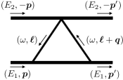
Figure 15: The triangle diagram. The thick and thin lines represent massive and massless particles, respectively.

As a warm up, we study a general triangle diagram, defined here to be a one-loop integral comprised of an arbitrary numerator together with one $\phi_{1}$ propagator and two graviton propagators arranged as in Fig. 15. In the notation of Eq. (7.1), the corresponding integrand takes the form

$${\cal I}_{\rm T} =\frac{1}{(E_{1}+\omega)^{2}-(\bm{p}+\bm{\ell})^{2}-m_{1}^{2}}\,\frac{1}{\omega^{2}-\bm{\ell}^{2}}\,\frac{1}{\omega^{2}-(\bm{\ell}+\bm{q})^{2}}\,{\cal N}_{\rm T}\,.$$ (7.11)

First we determine the effective numerator. The scalar propagators can be factored into matter and antimatter components,

$$\frac{1}{(E_{1}+\omega)^{2}-(\bm{p}+\bm{\ell})^{2}-m_{1}^{2}}=\frac{1}{(\omega-\omega_{P_{1}})(\omega-\omega_{A_{1}})}\,,\qquad\omega_{P_{1}},\omega_{A_{1}}=-E_{1}\pm\sqrt{E_{1}^{2}+2\bm{p}\bm{\ell}+\bm{\ell}^{2}}\,.$$ (7.12)

Thus, the spatial integrand is given in terms of the effective numerator by

$$\widetilde{\cal I}_{{\rm T}}=\int\frac{d\omega}{2\pi}\,\frac{\widetilde{\cal N}_{\rm T}(\omega)}{\omega-\omega_{P_{1}}}\,,\qquad\widetilde{\cal N}_{\rm T}(\omega)=\frac{1}{\omega-\omega_{A_{1}}}\,\frac{1}{\omega^{2}-\bm{\ell}^{2}}\,\frac{1}{\omega^{2}-(\bm{\ell}+\bm{q})^{2}}\,{\cal N}_{\rm T}(\omega)\,,$$ (7.13)

where for emphasis we have made explicit all dependence on $\omega$.

Second we use energy-integral reduction to evaluate the energy integral. From Eq. (7.13), we see that any numerator term which cancels the $\omega-\omega_{P_{1}}$ pole leads to a scaleless integral. Thus, the general constraint in Eq. (7.7) for this example is simply

$$\omega-\omega_{P_{1}}\rightarrow 0\,.$$ (7.14)

Applying this replacement is of course equivalent to sending

$$\widetilde{\cal N}_{\rm T}(\omega)\rightarrow\widetilde{\cal N}_{\rm T}(\omega_{P_{1}})\,.$$ (7.15)

The spatial integrand then takes the form

$$\widetilde{\cal I}_{\rm T}=\widetilde{\cal N}_{\rm T}(\omega_{P_{1}})\int\frac{d\omega}{2\pi}\frac{1}{\omega-\omega_{P_{1}}}\,.$$ (7.16)

The energy integral has no more energy dependence in the numerator, and we identify this as the triangle master energy integral.

The triangle master energy integral can be computed in various ways which will be instructive when we eventually encounter more complicated objects. The first option is to compute the integral by direct evaluation on a symmetric interval:

$$\int\frac{d\omega}{\omega-\omega_{P_{1}}+i\epsilon}\equiv\lim_{R\rightarrow\infty}\int\limits_{-R}^{R}\frac{d\omega}{\omega-\omega_{P_{1}}+i\epsilon}=\frac{1}{2}\times(-2\pi i)\,,$$ (7.17)

where on the left hand side we have reintroduced the appropriate $i\epsilon$ to regularize the integral coming from the original propagators, following the standard Feynman $i\epsilon$ prescription in Eq. (7.12). A heuristic for the sign in front of the $i\epsilon$ is that it designates whether positive $\omega$ increases or decreases the energy of the matter particle corresponding to this pole. We have expressed our answer in terms of a 1/2 symmetry factor multiplying the quantity one would naively extract from computing the residue on the matter pole including signs.

One approach is to compute the master energy integral directly via residues. At one loop there is a single integration variable and the analysis is straightforward CliffIraMikhailClassical . This is not the case for multivariable integration. Pushing the contour of integration into the upper half complex plane, we pick up the residue at $\omega=\omega_{P_{1}}-i\epsilon$ as well as the contribution from the upper half arc at infinity. Pushing the contour down, there are no residues to pick up but we include the contribution from the lower-half arc at infinity. Averaging over the two equivalent prescriptions, the half-arc contributions cancel and we are again left with the 1/2 symmetry factor relative to the residue on the matter pole.

The following approach will be our standard method of choice since it scales nicely to higher loop. First we assign to each graviton a unique energy component $\omega_{i}$ with $i=1$ to $n_{G}$. Then we introduce delta functions to rewrite the expression as an integral over a subset of the $n_{G}$ loop energy variables. Finally, we average over permutations of the loop energies that preserve isometries of the delta functions. If the resulting integrand is such that it vanishes in the $i\epsilon\to 0$ limit, then we have a convergent integral that can be directly performed. Applying this to the triangle gives

$$\int\frac{d\omega}{\omega-\omega_{P_{1}}+i\epsilon} \equiv\int d\omega_{1}\,d\omega_{2}\,\delta(\omega_{1}+\omega_{2})\frac{1}{2!}\left[\frac{1}{\omega_{1}-\omega_{P_{1}}+i\epsilon}+\frac{1}{\omega_{2}-\omega_{P_{1}}+i\epsilon}\right]$$ (7.18)

$$=\frac{1}{2}\int\left(\frac{d\omega}{\omega-\omega_{P_{1}}+i\epsilon}+\frac{d\omega}{-\omega-\omega_{P_{1}}+i\epsilon}\right)=\frac{1}{2}\times(-2\pi i)\,,$$

where in the final equality we have evaluated the integral over the real domain, which is well-defined and yields the 1/2 symmetry factor.

The purpose of the symmetrization procedure is to make the integrand manifestly convergent. Without symmetrization, the original integrand scales as $1/\omega$ at large $\omega$ and thus receives boundary contributions at infinity. By symmetrizing over two equivalent energy routings, we obtain a new integrand that falls of manifestly as $1/\omega^{2}$ and has no contribution at infinity. The same feature will emerge in all of our other examples which include triangle subdiagrams. In the soft eikonal expansion, it is known that this type of averaging over graviton permutations effectively eliminates the singular “principal value” contribution that arises when $i\epsilon$ is set to zero StermanEikonal ; BjerrumClassical .

Finally, we evaluate the spatial integral. After carrying out the energy integral we obtain

$$\widetilde{\cal I}_{\rm T}(\bm{p},\bm{q},\bm{\ell})=-\frac{i}{2}\,\frac{1}{\omega_{P_{1}}-\omega_{A_{1}}}\,\frac{1}{\omega_{P_{1}}^{2}-\bm{\ell}^{2}}\,\frac{1}{\omega_{P_{1}}^{2}-(\bm{\ell}+\bm{q})^{2}}\,{\cal N}_{\rm T}(\omega_{P_{1}})\,.$$ (7.19)

Note that $\widetilde{\cal I}_{\rm T}$ is a quite complicated function of $\bm{p}$, $\bm{q}$, and $\bm{\ell}$ since $\omega_{P_{1}}$ and $\omega_{A_{1}}$ contain square root functions. As a result, direct integration would be difficult. We therefore first expand the spatial integrand in the nonrelativistic limit, $|\bm{p}|\ll m_{1},m_{2}$. In this limit the various denominators become

$$\frac{1}{\omega_{P_{1}}-\omega_{A_{1}}} =\frac{1}{2m_{1}}+\cdots\,,$$ (7.20)

$$\frac{1}{\omega_{P_{1}}^{2}-\bm{\ell}^{2}} =-\frac{1}{\bm{\ell}^{2}}+\cdots\,,$$

$$\frac{1}{\omega_{P_{1}}^{2}-(\bm{\ell}+\bm{q})^{2}} =-\frac{1}{(\bm{\ell}+\bm{q})^{2}}+\cdots\,.$$

Thus we see that, in the nonrelativistic expansion of $\widetilde{\cal I}_{\rm T}$, the only singularities arise from powers of $\bm{\ell}^{2}$ and $(\bm{\ell}+\bm{q})^{2}$ in the denominator. Consequently $\widetilde{\cal I}_{\rm T}$ takes exactly the form of Eq. (7.8) with $\gamma=0$ and can thus be evaluated straightforwardly using Eq. (7.9).

As a concrete illustration, consider the scalar triangle integral for which ${\cal N}_{\rm T}=1$. From relativistic considerations it is obvious that the scalar triangle integral is only a function of $\bm{q}^{2}$ and $m_{1}^{2}$ since these are the only invariants that can be formed. Hence the scalar triangle integral must be a series expansion in $|\bm{q}|/m_{1}$, and the classical contribution is entirely given by the first term

$$\widetilde{\cal I}_{\rm T}(\bm{p},\bm{q},\bm{\ell})=-\frac{i}{4m_{1}\bm{\ell}^{2}(\bm{\ell}+\bm{q})^{2}}\,.$$ (7.21)

By direct integration with Eq. (7.9), we obtain the known result for the classical part of the one-loop triangle diagram

$$I_{\rm T} =-\frac{i}{32m_{1}|\bm{q}|}\,.$$ (7.22)

Note that this result is not the full relativistic scalar triangle integral, but rather the leading classical contribution arising from exchanges of potential gravitons. This is derived as well using Mellin-Barnes integration in Sec. 8.2.

7.2.2 Box Diagram

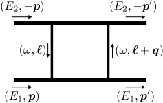
Figure 16: The one-loop box diagram. The thick and thin lines represent massive and massless particles, respectively.

The next simplest example is the box diagram, defined as an arbitrary numerator together with one $\phi_{1}$ propagator, one $\phi_{2}$ propagator, and two graviton propagators as shown in Fig. 16. Since the numerator is arbitrary, this example has as a subcase the triangle diagram. The box integrand is

$${\cal I}_{\rm B} =\frac{1}{(E_{1}+\omega)^{2}-(\bm{p}+\bm{\ell})^{2}-m_{1}^{2}}\,\frac{1}{(E_{2}-\omega)^{2}-(\bm{p}+\bm{\ell})^{2}-m_{2}^{2}}\,\frac{1}{\omega^{2}-\bm{\ell}^{2}}\,\frac{1}{\omega^{2}-(\bm{\ell}+\bm{q})^{2}}\,{\cal N}_{\rm B}\,.$$ (7.23)

As before, we split the scalar propagators into matter and antimatter components, obtaining Eq. (7.12) together with the analogous formula for the second massive propagator

$$\frac{1}{(E_{2}-\omega)^{2}-(\bm{p}+\bm{\ell})^{2}-m_{2}^{2}} =\frac{1}{(\omega-\omega_{P_{2}})(\omega-\omega_{A_{2}})}\,,\qquad\omega_{P_{2}},\omega_{A_{2}}=E_{2}\mp\sqrt{E_{2}^{2}+2\bm{p}\bm{\ell}+\bm{\ell}^{2}}\,.$$ (7.24)

The spatial integrand is then given in terms of the effective numerator by

$$\widetilde{\cal I}_{\rm B}=\int\frac{d\omega}{2\pi}\,\frac{\widetilde{\cal N}_{\rm B}(\omega)}{(\omega-\omega_{P_{1}})(\omega-\omega_{P_{2}})}\,,$$ (7.25)

where

$$\widetilde{\cal N}_{\rm B}(\omega) =\frac{1}{\omega-\omega_{A_{1}}}\frac{1}{\omega-\omega_{A_{2}}}\,\frac{1}{\omega^{2}-\bm{\ell}^{2}}\,\frac{1}{\omega^{2}-(\bm{\ell}+\bm{q})^{2}}\,{\cal N}_{\rm B}(\omega)\,.$$ (7.26)

Next, we apply energy-integral reduction to recast the integrand in terms of a set of master energy integrals. Since simultaneously eliminating both poles in $\widetilde{\cal I}_{\rm B}$ produces a scaleless energy integral, the general constraint in Eq. (7.7) for this example is given by

$$(\omega-\omega_{P_{1}})(\omega-\omega_{P_{2}})\rightarrow 0\,.$$ (7.27)

The constraint in Eq. (7.27) defines the zero locus for a certain quadratic polynomial in $\omega$. Note how this contrasts with the simpler linear constraint we saw earlier in Eq. (7.14). Previously, to evaluate the effective numerator on the linear constraint it sufficed to trivially plug in for the single solution for $\omega$. However, imposing the quadratic constraint in Eq. (7.27) is more involved. In particular, Eq. (7.27) does not indicate that we can set either $\omega=\omega_{P_{1}}$ or $\omega=\omega_{P_{2}}$ in the numerator. Instead, the claim is that any time the full quadratic function in Eq. (7.27) appears in the effective numerator, we can drop it. This is required because only if both matter poles, $\omega-\omega_{P_{1}}$ and $\omega-\omega_{P_{2}}$, are canceled do we have a scaleless integral that can be dropped, cf. Eq. (7.6).

To apply energy reduction on the effective numerator we simply compute the remainder of $\widetilde{\cal N}_{\rm B}$ under modular division by the quadratic polynomial in Eq. (7.27). If $\widetilde{\cal N}_{\rm B}$ were a polynomial, e.g. obtained by expanding Eq. (7.27) as a series expansion in $\omega$ up to some high order, then it is obvious how to perform this modular division, i.e., simply by repeated application of Eq. (7.27). However, if we want to retain Eq. (7.25) to all orders, then the effective numerator is not simply a polynomial in $\omega$ but has complicated denominator poles. Nevertheless, we can still perform modular division by the following procedure. First we shift the integration variable $\omega$ such that the constraint in Eq. (7.27) is of the form $\omega^{2}-\zeta=0$, where $\zeta$ is a constant. Then we express $\widetilde{\cal N}_{\rm B}$ in terms of even and odd functions in $\omega$, whose denominators are even in $\omega$. Then all appearances of $\omega^{2}$ can simply be set to $\zeta$. In particular, the even functions become constants, while the odd functions become linear in $\omega$. In this way, an arbitrary numerator is reduced to the form

$$\widetilde{\cal N}_{\rm B}(\omega)\rightarrow f_{0}+f_{1}\omega\,.$$ (7.28)

Next, we consider further expanding this linear function for $\widetilde{\cal N}_{\rm B}(\omega)$ about the point $\omega_{P_{1}}$, so there is a term proportional to $\omega-\omega_{P_{1}}$ and a remainder term. The former will cancel one of the matter poles, yielding an expression of the form of the triangle diagram tackled in the previous section. Meanwhile, the latter is a new ingredient since it does not cancel any of the matter poles. This contribution yields the box master energy integral. As before, we evaluate it by averaging over the two permutations of the graviton labels,

$$\int\frac{d\omega}{(\omega-\omega_{P_{1}}+i\epsilon)(\omega-\omega_{P_{2}}-i\epsilon)} =\frac{1}{2}\int\left(\frac{d\omega_{1}d\omega_{2}\delta(\omega_{1}+\omega_{2})}{(\omega_{1}-\omega_{P_{1}}+i\epsilon)(\omega_{1}-\omega_{P_{2}}-i\epsilon)}+\{\omega_{1}\leftrightarrow-\omega_{2}\}\right)$$ (7.29)

$$=\frac{1}{\omega_{P_{1}}-\omega_{P_{2}}}\times(-2\pi i)\,,$$

where again we use the standard Feynman $i\epsilon$ prescription. This agrees with the heuristic mentioned earlier, which assigns opposite signs to each $i\epsilon$ factor since for the box, increasing $\omega$ will increase the energy of one matter line and decrease that of the other. Here we have symmetrized over routings of the loop energies to parallel our earlier analysis, but since the original integrand falls off as $1/\omega^{2}$ it is also straightforward to evaluate it via contour integration without symmetrization.

In the above discussion we made the choice of expanding $\widetilde{\cal N}_{\rm B}(\omega)$ about $\omega_{P_{1}}$, and we obtained contributions from the master triangle and master box energy integrals. Both contributions must be included to obtain the correct answer. Alternatively, we could have chosen to expand about the point $\omega_{P_{2}}$ instead, in which case the various integrals would slightly change but yield the same final answer.

The important feature of Eq. (7.29) is that it introduces a new kind of singularity coming from the $(\omega_{P_{2}}-\omega_{P_{1}})$ denominator factor. For example, expanding in the classical limit using the scaling $(\bm{\ell}^{2}+2\bm{p}\bm{\ell})\sim{\cal O}(\bm{q})$, this pole becomes

$$\frac{1}{\omega_{P_{1}}-\omega_{P_{2}}}=\frac{2E_{1}E_{2}}{E_{1}+E_{2}}\,\frac{1}{2\bm{p}\bm{\ell}+\bm{\ell}^{2}}+\cdots\,,$$ (7.30)

which is singular when the internal $\phi_{1}$ and $\phi_{2}$ particles are on shell. The ellipsis here denotes terms higher order in $(\bm{\ell}^{2}+2\bm{p}\bm{\ell})$, which may contribute to the final classical result.

As an example consider the scalar box integral for which ${\cal N}_{\rm B}=1$. Applying the procedure described above, we obtain the spatial integrand

$$\widetilde{\cal I}_{\rm B} ={i\over 2E\bm{\ell}^{2}(\bm{\ell}+\bm{q})^{2}(\bm{\ell}^{2}+2\bm{p}\bm{\ell})}+{i(E_{1}^{2}-3E_{2}^{2})\left(\bm{\ell}^{2}(\bm{\ell}+\bm{q})^{2}-(\bm{\ell}^{2}+(\bm{\ell}+\bm{q})^{2})(\bm{\ell}^{2}+2\bm{p}\bm{\ell})\right)\over 16E_{1}^{2}E_{2}^{2}E\bm{\ell}^{4}(\bm{\ell}+\bm{q})^{4}}$$ (7.31)

$$-{i(E_{1}^{4}-3E_{2}^{4})\left[(\bm{\ell}^{4}+\bm{\ell}^{2}(\bm{\ell}+\bm{q})^{2}+(\bm{\ell}+\bm{q})^{4})(\bm{\ell}^{2}+2\bm{p}\bm{\ell})-3\bm{\ell}^{2}(\bm{\ell}+\bm{q})^{2}(\bm{\ell}^{2}+(\bm{\ell}+\bm{q})^{2})\right](\bm{\ell}^{2}+2\bm{p}\bm{\ell})^{2}\over 64E_{1}^{4}E_{2}^{4}E\bm{\ell}^{6}(\bm{\ell}+\bm{q})^{6}}$$

$$+\cdots\,,$$

where the asymmetry in the labels 1 and 2 is due to the choice of expanding about $\omega_{P_{1}}$. The final answer below is symmetric in the labels 1 and 2, as it should be. To obtain Eq. (7.31) we performed two expansions. First, we expanded in the classical limit of large angular momentum $J$, or equivalently small momentum $\bm{q}$, using the scalings $\bm{\ell}\sim(\bm{\ell}+\bm{q})\sim(\bm{\ell}^{2}+2\bm{p}\bm{\ell})\sim{\cal O}(\bm{q})$. Second, we expanded in the nonrelativistic limit, but keeping existing energy factors intact. By direct integration of Eq. (7.31) using Eq. (7.9), we obtain

$$I_{\rm B} =\int\frac{d^{D-1}\bm{\ell}}{(2\pi)^{D-1}}\,{i\over 2E\bm{\ell}^{2}(\bm{\ell}+\bm{q})^{2}(\bm{\ell}^{2}+2\bm{p}\bm{\ell})}\,,$$ (7.32)

where the classical terms vanish order by order in the nonrelativistic expansion. The terms in Eq. (7.31) that are antisymmetric in the labels 1 and 2 have vanished. The above remaining integral has the form of Eq. (7.8) with $\gamma=1$. It is infrared divergent and superclassical, having an additional factor of $|\bm{q}|^{-1}$ relative to the classical scaling. As noted previously, we choose not to evaluate these quantities explicitly since they are IR artifacts that are guaranteed to subtract exactly with matching contributions from the EFT amplitude.

7.2.3 Crossed-Box Diagram

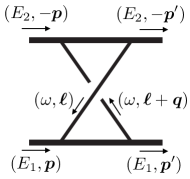
Figure 17: The crossed-box diagram.

Next, consider the crossed box diagram, defined as an arbitrary numerator together with one $\phi_{1}$ propagator, one $\phi_{2}$ propagator, and two graviton propagators as shown in Fig. 17. The integrand of the crossed-box diagram is

$${\cal I}_{\overline{\rm B}} =\frac{1}{(E_{1}+\omega)^{2}-(\bm{p}+\bm{\ell})^{2}-m_{1}^{2}}\,\frac{1}{(E_{2}+\omega)^{2}-(\bm{p}-\bm{\ell}-\bm{q})^{2}-m_{2}^{2}}\,\frac{1}{\omega^{2}-\bm{\ell}^{2}}\,\frac{1}{\omega^{2}-(\bm{\ell}+\bm{q})^{2}}\,{\cal N}_{\overline{\rm B}}\,.$$ (7.33)

The analysis here is almost identical to the box integral. We again apply energy-integral reduction, exploiting the fact that when the energy denominators for both the $\phi_{1}$ and $\phi_{2}$ propagators are canceled, then the resulting scaleless energy integral is quantum and can be discarded. As for the box integral, we will obtain contributions proportional to the master triangle energy integral. The only difference from the box is that upon energy-integral reduction, we obtain another new crossed box master energy integral,

$$\int\frac{d\omega}{(\omega-\omega_{P_{1}}+i\epsilon)(\omega-\omega_{P_{2}}+i\epsilon)} =\frac{1}{2}\int\left(\frac{d\omega}{(\omega-\omega_{P_{1}}+i\epsilon)(\omega-\omega_{P_{2}}+i\epsilon)}+\{\omega\leftrightarrow-\omega\}\right)=0\,.$$ (7.34)

Note the same sign in front of each $i\epsilon$ factor. This occurs because for the crossed box, increasing $\omega$ will increase the energy flow through both matter propagators. Crucially, this slight difference means that the crossed-box master energy integral is zero.

This vanishing can be understood by deforming the integration contour. The integrand in Eq. (7.34) obviously vanishes at infinity, so by closing the contour of integration into the upper half plane, we obtain zero. This type of cancellation is the calling card for contributions which vanish due to causality in nonrelativistic field theory. There is a simple diagrammatic diagnostic to determine which energy integrals are zero. Since every graviton of interest is a potential mode, it connects two points of equal time. We can then divide all topologies according to whether they are connected or disconnected after cutting all matter lines. For connected diagrams, like the triangle, all vertices connected to a graviton are simultaneous interactions. Meanwhile, disconnected diagrams like the box and crossed box can be thought of describing a series of two simultaneous events, corresponding to each graviton exchange. Any two events must occur in some time order. If we then draw the worldlines of the scalar fields for the box and crossed box, we then see that the latter requires backwards in time propagating matter particles, i.e. antimatter, to be consistent. Consequently these diagrams vanish by causality.

We now briefly discuss the scalar example, setting ${\cal N}_{\overline{\rm B}}=1$. Applying energy-integral reduction gives a contribution proportional to the crossed-box master integral and a contribution proportional to the triangle master integral. The former vanishes since the crossed-box master integral is zero, while the latter vanishes by direct integration of the spatial integrand, order by order in the velocity expansion. Hence, the scalar crossed-box diagram has no classical contribution.

The vanishing of classical contributions from the sum of the box and crossed-box diagrams can be shown to all orders using other integration methods, such as direct integration of the soft region or the use of differential equations. Our focus here is to illustrate the application of our nonrelativistic integration procedure.

7.3 Two-Loop Examples

We are now prepared to consider some examples at two loops. As advertised, our methodology will be identical to the one-loop cases, only here applied sequentially to each loop.

7.3.1 Double-Triangle Diagram

To begin, consider the general double-triangle diagram, which is a two-loop integral with an arbitrary numerator together with two $\phi_{1}$ propagators and three graviton propagators arranged as in Fig. 18.

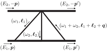
Figure 18: The double-triangle diagram.

The integrand corresponding to this diagram is

$${\cal I}_{{\rm TT}}= \frac{1}{(E_{1}+\omega_{1})^{2}-(\bm{p}+\bm{\ell}_{1})^{2}-m_{1}^{2}}\,\frac{1}{(E_{1}+\omega_{1}+\omega_{2})^{2}-(\bm{p}+\bm{\ell}_{1}+\bm{\ell}_{2})^{2}-m_{1}^{2}}$$ (7.35)

$$\times\frac{1}{\omega_{1}^{2}-\bm{\ell}_{1}^{2}}\,\frac{1}{\omega_{2}^{2}-\bm{\ell}_{2}^{2}}\,\frac{1}{(\omega_{1}+\omega_{2})^{2}-(\bm{\ell}_{1}+\bm{\ell}_{2}+\bm{q})^{2}}\,{\cal N}_{\rm TT}\,.$$

Both $\phi_{1}$ propagators can be factored into matter and antimatter components,

$$\frac{1}{(E_{1}+\omega)^{2}-(\bm{p}+\bm{\ell})^{2}-m_{1}^{2}} =\frac{1}{(\omega_{1}-\omega_{P_{1}})(\omega_{1}-\omega_{A_{1}})}\,,$$ (7.36)

$$\frac{1}{(E_{1}+\omega_{1}+\omega_{2})^{2}-(\bm{p}+\bm{\ell}_{1}+\bm{\ell}_{2})^{2}-m_{1}^{2}} =\frac{1}{(\omega_{1}+\omega_{2}-\omega_{P_{1}^{\prime}})(\omega_{1}+\omega_{2}-\omega_{A_{1}^{\prime}})}\,.$$

The spatial integrand is then given in terms of the effective numerator by

$$\widetilde{\cal I}_{{\rm TT}} =\int\frac{d\omega_{1}}{2\pi}\frac{d\omega_{2}}{2\pi}\,\frac{\widetilde{\cal N}_{\rm TT}(\omega_{1},\omega_{2})}{(\omega_{1}-\omega_{P_{1}})(\omega_{1}+\omega_{2}-\omega_{P_{1}^{\prime}})}\,,$$ (7.37)

where

$$\widetilde{\cal N}_{\rm TT}(\omega_{1},\omega_{2}) =\frac{1}{\omega_{1}-\omega_{A_{1}}}\,\frac{1}{\omega_{1}+\omega_{2}-\omega_{A_{1}^{\prime}}}\,\frac{1}{\omega_{1}^{2}-\bm{\ell}_{1}^{2}}\,\frac{1}{\omega_{2}^{2}-\bm{\ell}_{2}^{2}}\,\frac{1}{(\omega_{1}+\omega_{2})^{2}-(\bm{\ell}_{1}+\bm{\ell}_{2}+\bm{q})^{2}}\,{\cal N}_{\rm TT}(\omega_{1},\omega_{2})\,.$$ (7.38)

Next, we use the fact that canceling either energy denominator will produce a scaleless integral in either $\omega_{1}$ or $\omega_{2}$. Consequently, we can freely send

$$\omega_{1}-\omega_{P_{1}}\rightarrow 0\,,\qquad\omega_{1}+\omega_{2}-\omega_{P_{1}^{\prime}}\rightarrow 0\,,$$ (7.39)

so we can effectively evaluate the numerator

$$\widetilde{\cal N}_{\rm TT}(\omega_{1},\omega_{2})\rightarrow\widetilde{\cal N}_{\rm TT}(\omega_{P_{1}},\omega_{P_{1}^{\prime}}-\omega_{P_{1}})\,.$$ (7.40)

Upon this replacement, the spatial integrand becomes

$$\widetilde{\cal I}_{\rm TT} =\widetilde{\cal N}_{\rm TT}(\omega_{P_{1}},\omega_{P_{1}^{\prime}}-\omega_{P_{1}})\int\frac{d\omega_{1}}{2\pi}\frac{d\omega_{2}}{2\pi}\,\frac{1}{(\omega_{1}-\omega_{P_{1}})(\omega_{1}+\omega_{2}-\omega_{P_{1}^{\prime}})}\,.$$ (7.41)

Here the last factor is the double-triangle master energy integral. We evaluate it by averaging over permutations of labelings of the three exchanged gravitons,

$$\int\frac{d\omega_{1}\,d\omega_{2}}{(\omega_{1}-\omega_{P_{1}}+i\epsilon)(\omega_{1}+\omega_{2}-\omega_{P_{1}^{\prime}}+i\epsilon)} \equiv\frac{1}{3!}\left(\int\frac{d\omega_{1}\,d\omega_{2}}{(\omega_{1}-\omega_{P_{1}}+i\epsilon)(\omega_{1}+\omega_{2}-\omega_{P_{1}^{\prime}}+i\epsilon)}+\{\textrm{perm.}\}\right)$$ (7.42)

$$=\frac{1}{6}\times(-2\pi i)^{2}\,,$$

where we include all permutations of $\omega_{1}$, $\omega_{2}$, and $\omega_{3}$, and we set $\omega_{3}=-\omega_{1}-\omega_{2}$ by energy conservation in the end. Again we use the standard Feynman $i\epsilon$ prescription, which agrees with the same heuristic as before: we include the same sign in front of each $i\epsilon$ factor since increasing $\omega_{1}$ increases the energy flowing through each matter line. By explicit calculation we have obtained a 1/6 symmetry factor relative to the naive expression one would obtain by sequential application of the residue theorem on each pole.

As before, the original integrand scales as $1/\omega_{2}$ at infinity, but the symmetrization improves the asymptotic behavior to $1/\omega_{2}^{2}$ so there is no boundary term to consider and integration is mechanical.

Having evaluated the energy integral, we obtain the spatial integrand

$$\widetilde{\cal I}_{\rm TT}(\bm{p},\bm{q},\bm{\ell}_{1},\bm{\ell}_{2}) =\frac{1}{\omega_{P_{1}}-\omega_{A_{1}}}\,\frac{1}{\omega_{P_{1}^{\prime}}-\omega_{A_{1}^{\prime}}}\,\frac{1}{\omega_{P_{1}}^{2}-\bm{\ell}_{1}^{2}}\,\frac{1}{(\omega_{P_{1}^{\prime}}-\omega_{P_{1}})^{2}-\bm{\ell}_{2}^{2}}\,\frac{1}{\omega_{P_{1}^{\prime}}^{2}-(\bm{\ell}_{1}+\bm{\ell}_{2}+\bm{q})^{2}}$$ (7.43)

$$\qquad\times{\cal N}_{\rm TT}(\omega_{P_{1}},\omega_{P_{1}^{\prime}}-\omega_{P_{1}})\times\left(-\frac{1}{6}\right).$$

As before, consider for illustration the simple case of the scalar double-triangle integral, for which ${\cal N}_{\rm TT}=1$. Expanding the spatial integrand in the nonrelativistic limit, ${\bm{p}}\ll m_{1,2}$, implemented here as $m_{1}\rightarrow\infty$, we obtain

$$\widetilde{\cal I}_{\rm TT}(\bm{p},\bm{q},\bm{\ell}_{1},\bm{\ell}_{2})={1\over 24m_{1}^{2}{\bm{\ell}_{1}}^{2}{\bm{\ell}_{2}}^{2}{(\bm{\ell}_{1}+\bm{\ell}_{2}+\bm{q})}^{2}}\,.$$ (7.44)

As in the case of the one-loop triangle, the scalar double-triangle integral is only a function of $\bm{q}^{2}$ and $m_{1}^{2}$, since these are the only rotational invariants that can be constructed from the momenta flowing into the integral. For this reason, we know that the integral is a series expansion in $\bm{q}^{2}/m_{1}^{2}$, and we have kept only the classical term in Eq. (7.44).

We immediately see that the dependence on both $\bm{\ell}_{1}$ and $\bm{\ell}_{2}$ is of the form of Eq. (7.8), which follows trivially since the double triangle is made entirely of triangle subdiagrams. Applying Eq. (7.9) sequentially to each integral, we obtain our final result for the classical contribution from the scalar double-triangle integral to all orders in velocity,

$$I_{\rm TT} =-\frac{1}{768\pi^{2}m_{1}^{2}}\ln\bm{q}^{2}\,.$$ (7.45)

This is also derived using Mellin-Barnes integration in Sec. 8.2.

In obtaining Eq. (7.45) we used the general formula in Eq. (7.9) applied to this example,

$$\int\frac{d^{D-1}\bm{\ell}}{(2\pi)^{D-1}}\,\frac{1}{|\bm{\ell}|(\bm{\ell}+\bm{q})^{2}}=\frac{1}{4\pi^{2}\epsilon}-\frac{1}{4\pi^{2}}\ln{{\bm{q}}^{2}\over\mu^{2}}\,,$$ (7.46)

where we employ dimensional regularization in $D=4-2\epsilon$ and the $\overline{\hbox{MS}}$ scheme. The $\ln\bm{q}^{2}$ term is the classical contribution at two-loop order since its Fourier transform to position space is $\left[G^{3}\ln\bm{q}^{2}\right]_{\rm FT}=-{1\over 2\pi}\left({G\over|{\bm{r}}|}\right)^{3}$. Crucially all terms that are constant in ${\bm{q}}$, such as the $1/\epsilon$ and $\ln\mu^{2}$ terms, are contact terms whose Fourier transforms to position space yield $\delta(|{\bm{r}}|)$. Hence they do not contribute to the long-distance classical potential. These ultraviolet-sensitive contributions are quantum mechanical, and can be absorbed into an appropriate counterterm.

7.3.2 Double-Triangle Prime Diagram

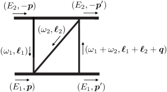
Figure 19: The double-triangle prime diagram.

Consider next the double-triangle-prime diagram, which is a two-loop integral with an arbitrary numerator together with one $\phi_{1}$ propagator, one $\phi_{2}$ propagator, and three graviton propagators arranged as in Fig. 19. The integrand corresponding to this diagram is

$${\cal I}_{\rm TT^{\prime}}=\hbox{} \frac{1}{(E_{1}+\omega_{1}+\omega_{2})^{2}-(\bm{p}+\bm{\ell}_{1}+\bm{\ell}_{2})^{2}-m_{1}^{2}}\,\frac{1}{(E_{2}-\omega_{1})^{2}-(\bm{p}+\bm{\ell}_{1})^{2}-m_{2}^{2}}$$ (7.47)

$$\times\frac{1}{\omega_{1}^{2}-\bm{\ell}_{1}^{2}}\,\frac{1}{\omega_{2}^{2}-\bm{\ell}_{2}^{2}}\,\frac{1}{(\omega_{1}+\omega_{2})^{2}-(\bm{\ell}_{1}+\bm{\ell}_{2}+\bm{q})^{2}}\,{\cal N}_{\rm TT^{\prime}}\,.$$

Both $\phi_{1}$ and $\phi_{2}$ propagators can be factored into matter and antimatter components,

$$\frac{1}{(E_{1}+\omega_{1}+\omega_{2})^{2}-(\bm{p}+\bm{\ell}_{1}+\bm{\ell}_{2})^{2}-m_{1}^{2}} =\frac{1}{(\omega_{1}+\omega_{2}-\omega_{P_{1}})(\omega_{1}+\omega_{2}-\omega_{A_{1}})}\,,$$ (7.48)

$$\frac{1}{(E_{2}-\omega_{1})^{2}-(\bm{p}+\bm{\ell}_{1})^{2}-m_{2}^{2}} =\frac{1}{(\omega_{1}-\omega_{P_{2}})(\omega_{1}-\omega_{A_{2}})}\,.$$

The spatial integrand in terms of the effective numerator is then

$$\widetilde{\cal I}_{\rm TT^{\prime}} =\int\frac{d\omega_{1}}{2\pi}\frac{d\omega_{2}}{2\pi}\,\frac{\widetilde{\cal N}_{\rm TT^{\prime}}(\omega_{1},\omega_{2})}{(\omega_{1}-\omega_{P_{2}})(\omega_{1}+\omega_{2}-\omega_{P_{1}})}\,,$$ (7.49)

where

$$\widetilde{\cal N}_{\rm TT^{\prime}}(\omega_{1},\omega_{2}) =\frac{1}{\omega_{1}-\omega_{A_{2}}}\,\frac{1}{\omega_{1}+\omega_{2}-\omega_{A_{1}}}\,\frac{1}{\omega_{1}^{2}-\bm{\ell}_{1}^{2}}\,\frac{1}{\omega_{2}^{2}-\bm{\ell}_{2}^{2}}\,\frac{1}{(\omega_{1}+\omega_{2})^{2}-(\bm{\ell}_{1}+\bm{\ell}_{2}+\bm{q})^{2}}\,{\cal N}_{\rm TT^{\prime}}(\omega_{1},\omega_{2}).$$ (7.50)

Next, we use the fact that canceling either energy denominator will produce a scaleless integral in either $\omega_{1}$ or $\omega_{2}$. Consequently, we can freely send

$$\omega_{1}-\omega_{P_{2}}\rightarrow 0\qquad{\rm and}\qquad\omega_{1}+\omega_{2}-\omega_{P_{1}}\rightarrow 0\,,$$ (7.51)

so we can effectively evaluate the numerator

$$\widetilde{\cal N}_{\rm TT^{\prime}}(\omega_{1},\omega_{2})\rightarrow\widetilde{\cal N}_{\rm TT^{\prime}}(\omega_{P_{2}},\omega_{P_{1}}-\omega_{P_{2}})\,.$$ (7.52)

Upon this replacement, the spatial integrand becomes

$$\widetilde{\cal I}_{\rm TT^{\prime}} =\widetilde{\cal N}_{\rm TT^{\prime}}(\omega_{P_{2}},\omega_{P_{1}}-\omega_{P_{2}})\int\frac{d\omega_{1}}{2\pi}\frac{d\omega_{2}}{2\pi}\,\frac{1}{(\omega_{1}-\omega_{P_{2}})(\omega_{1}+\omega_{2}-\omega_{P_{1}})}\,.$$ (7.53)

Here the last factor is the double-triangle prime master energy integral. As before, we evaluate it by averaging over permutations of labelings of the three exchanged gravitons,

$$\int\frac{d\omega_{1}\,d\omega_{2}}{(\omega_{1}-\omega_{P_{1}}+i\epsilon)(\omega_{1}+\omega_{2}-\omega_{P_{1}^{\prime}}-i\epsilon)} \equiv\frac{1}{3!}\left(\int\frac{d\omega_{1}\,d\omega_{2}}{(\omega_{1}-\omega_{P_{1}}+i\epsilon)(\omega_{1}+\omega_{2}-\omega_{P_{1}^{\prime}}-i\epsilon)}+\{\textrm{perm.}\}\right)$$

$$=-\frac{1}{3}\times(-2\pi i)^{2}\,.$$ (7.54)

Note the sign difference in the $i\epsilon$ compared to the double-triangle master integral. By explicit calculation we have obtained a $-1/3$ symmetry factor relative to the naive expression one would obtain by sequential application of the residue theorem on each pole.

Having evaluated the energy integral, we obtain the spatial integrand,

$$\widetilde{\cal I}_{\rm TT^{\prime}}(\bm{p},\bm{q},\bm{\ell}_{1},\bm{\ell}_{2}) =\frac{1}{3}\widetilde{\cal N}_{\rm TT^{\prime}}(\omega_{P_{2}},\omega_{P_{1}}-\omega_{P_{2}})\,.$$ (7.55)

As before, we consider the simple case of a scalar integral for which ${\cal N}_{\rm TT^{\prime}}=1$. We proceed by expanding the integrand in the classical limit and dropping the quantum contributions. Then to put the integrand in the form of Eq. (7.8), we may expand in the nonrelativistic limit implemented as $m_{1,2}\to\infty$ as before. Alternatively, we choose instead to expand in $E_{1,2}\to\infty$ in order to keep the functions of $\sqrt{{\bm{p}}^{2}+m_{i}^{2}}$ intact. Unlike the double-triangle integral, this integral depends on the invariant $p_{1}\cdot p_{2}=E_{1}E_{2}+\bm{p}^{2}$. Expanding the spatial integrand this way, we obtain

$$\widetilde{\cal I}_{\rm TT^{\prime}} ={1\over 12E_{1}E_{2}{\bm{\ell}_{1}^{2}}(\bm{\ell}_{2}-\bm{\ell}_{1})^{2}(\bm{\ell}_{2}+\bm{q})^{2}}\bigg{[}1+{(\bm{\ell}_{1}^{2}+2\bm{p}\bm{\ell}_{1})^{2}\over 4E_{2}^{2}{\bm{\ell}_{1}^{2}}}+{(\bm{\ell}_{1}^{2}+2\bm{p}\bm{\ell}_{1})^{2}\over 4E_{2}^{2}(\bm{\ell}_{2}-\bm{\ell}_{1})^{2}}$$ (7.56)

$$\quad+{(\bm{\ell}_{1}^{2}+2\bm{p}\bm{\ell}_{1})(\bm{\ell}_{2}^{2}+2\bm{p}\bm{\ell}_{2})\over 2E_{1}E_{2}(\bm{\ell}_{2}-\bm{\ell}_{1})^{2}}+{(\bm{\ell}_{2}^{2}+2\bm{p}\bm{\ell}_{2})^{2}\over 4E_{1}^{2}(\bm{\ell}_{2}-\bm{\ell}_{1})^{2}}+{(\bm{\ell}_{2}^{2}+2\bm{p}\bm{\ell}_{2})^{2}\over 4E_{1}^{2}(\bm{\ell}_{2}+\bm{q})^{2}}+\cdots\bigg{]}\,,$$

where we have shifted the integration variable $\bm{\ell}_{2}\to\bm{\ell}_{2}-\bm{\ell}_{1}$, and the ellipsis denotes higher-order terms in the nonrelativistic expansion. Applying Eq. (7.9) sequentially to each integral, we obtain

$$I_{\rm TT^{\prime}} =-\frac{\ln\bm{q}^{2}}{384\pi^{2}E_{1}E_{2}}\bigg{[}1+{\left(E_{1}^{3}+E_{2}^{3}\right)\over 3E_{1}^{2}E_{2}^{2}E}{\bm{p}}^{2}+\frac{\left(E_{1}^{5}+E_{2}^{5}\right)}{5E_{1}^{4}E_{2}^{4}E}{\bm{p}}^{4}+\frac{\left(E_{1}^{7}+E_{2}^{7}\right)}{7E_{1}^{6}E_{2}^{6}E}{\bm{p}}^{6}+\cdots\bigg{]}\,,$$ (7.57)

where $E=E_{1}+E_{2}$ and the ellipsis denotes higher-order terms in the nonrelativistic expansion. We have included in Eq. (7.57) results for higher-order terms not explicitly shown in Eq. (7.56), and have checked to sufficiently high orders that the obvious pattern persists, allowing us to resum (see Appendix C) the result as

$$I_{\rm TT^{\prime}} =-\frac{\ln\bm{q}^{2}}{192\pi^{2}m_{1}m_{2}}{{\rm arcsinh}\sqrt{{\sigma-1\over 2}}\over\sqrt{\sigma^{2}-1}}\,.$$ (7.58)

For later convenience we have defined the quantity

$$\sigma={p_{1}\cdot p_{2}\over m_{1}m_{2}}={E_{1}E_{2}+\bm{p}^{2}\over m_{1}m_{2}}\,,$$ (7.59)

where $p_{1}$ and $p_{2}$ are the incoming four-momenta associated with $\phi_{1}$ and $\phi_{2}$. In the nonrelativistic limit, $\sigma$ approaches unity.

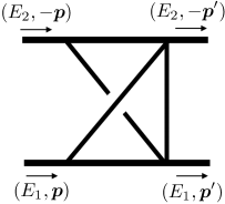
Figure 20: The nonplanar version of the double-triangle prime diagram.

The classical contribution from the scalar double-triangle prime integral is given to all orders in velocity in Eq. (7.58). As we cautioned at the end of Sec. 7.1, results for individual diagrams may be prescription dependent. Such is the case here, and only the sum of the double-triangle prime diagram with its nonplanar version can be unambiguously determined and compared to results obtained from other methods. Of course, our aim in this section is to illustrate the mechanics of our nonrelativistic integration method for general applicability, whether it be for a single diagram or for a sum of diagrams. Nonetheless, we briefly remark on the nonplanar diagram shown in Fig. 20. The calculation is similar to that of the planar case except that the symmetry factor is -1/6 instead of -1/3. The result is

$$I_{\overline{{\rm TT^{\prime}}}} =-\frac{\ln\bm{q}^{2}}{384\pi^{2}m_{1}m_{2}}{{\rm arcsinh}\sqrt{{\sigma-1\over 2}}\over\sqrt{\sigma^{2}-1}}\,.$$ (7.60)

The sum $I_{\rm TT^{\prime}}+I_{\overline{{\rm TT^{\prime}}}}$ agrees with the result from relativistic integration given in the first line of Eq. (8.14).

7.3.3 H and Crossed-H Diagrams

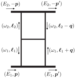
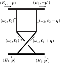
Figure 21: The H and crossed-H diagrams.

The next example we consider is the sum of the general H and crossed-H diagrams. We will denote the latter by ${\overline{\rm H}}$. These are two-loop integrals with arbitrary numerators and one $\phi_{1}$ propagator, one $\phi_{2}$ propagator, and five graviton propagators as shown in Fig. 21. The corresponding integrands are

$${\cal I}_{{\rm H}}= \frac{1}{(E_{1}+\omega_{1})^{2}-(\bm{p}+\bm{\ell}_{1})^{2}-m_{1}^{2}}\,\frac{1}{(E_{2}+\omega_{2})^{2}-(\bm{p}-\bm{\ell}_{2})^{2}-m_{2}^{2}}$$ (7.61)

$$\times\frac{1}{\omega_{1}^{2}-\bm{\ell}_{1}^{2}}\,\frac{1}{\omega_{1}^{2}-(\bm{\ell}_{1}+\bm{q})^{2}}\,\frac{1}{\omega_{2}^{2}-\bm{\ell}_{2}^{2}}\,\frac{1}{\omega_{2}^{2}-(\bm{\ell}_{2}-\bm{q})^{2}}\,\frac{1}{(\omega_{1}+\omega_{2})^{2}-(\bm{\ell}_{1}+\bm{\ell}_{2})^{2}}\,{\cal N}_{\rm H}\,,$$

$${\cal I}_{\overline{\rm H}}= \frac{1}{(E_{1}-\omega_{1})^{2}-(\bm{p}^{\prime}-\bm{\ell}_{1})^{2}-m_{1}^{2}}\,\frac{1}{(E_{2}+\omega_{2})^{2}-(\bm{p}-\bm{\ell}_{2})^{2}-m_{2}^{2}}$$

$$\times\frac{1}{\omega_{1}^{2}-\bm{\ell}_{1}^{2}}\,\frac{1}{\omega_{1}^{2}-(\bm{\ell}_{1}+\bm{q})^{2}}\,\frac{1}{\omega_{2}^{2}-\bm{\ell}_{2}^{2}}\,\frac{1}{\omega_{2}^{2}-(\bm{\ell}_{2}-\bm{q})^{2}}\,\frac{1}{(\omega_{1}+\omega_{2})^{2}-(\bm{\ell}_{1}+\bm{\ell}_{2})^{2}}\,{\cal N}_{\overline{\rm H}}\,.$$

As before the $\phi_{1}$ and $\phi_{2}$ propagators can be factored into matter and antimatter components,

$$\frac{1}{(E_{1}+\omega_{1})^{2}-(\bm{p}+\bm{\ell}_{1})^{2}-m_{1}^{2}} =\frac{1}{(\omega_{1}-\omega_{P_{1}})(\omega_{1}-\omega_{A_{1}})}\,,$$ (7.62)

$$\frac{1}{(E_{1}-\omega_{1})^{2}-(\bm{p}^{\prime}-\bm{\ell}_{1})^{2}-m_{1}^{2}} =\frac{1}{(\omega_{1}-\omega_{\overline{P}_{1}})(\omega_{1}-\omega_{\overline{A}_{1}})}\,,$$

$$\frac{1}{(E_{2}+\omega_{2})^{2}-(\bm{p}-\bm{\ell}_{2})^{2}-m_{2}^{2}} =\frac{1}{(\omega_{2}-\omega_{P_{2}})(\omega_{2}-\omega_{A_{2}})}\,.$$

The spatial integrands in terms of the effective numerator are then

$$\widetilde{\cal I}_{\rm H} =\int\frac{d\omega_{1}}{2\pi}\frac{d\omega_{2}}{2\pi}\,\frac{\widetilde{\cal N}_{\rm H}(\omega_{1},\omega_{2})}{(\omega_{1}-\omega_{P_{1}})(\omega_{2}-\omega_{P_{2}})}\,,$$ (7.63)

$$\widetilde{\cal I}_{\overline{\rm H}} =\int\frac{d\omega_{1}}{2\pi}\frac{d\omega_{2}}{2\pi}\,\frac{\widetilde{\cal N}_{\overline{\rm H}}(\omega_{1},\omega_{2})}{(\omega_{1}-\omega_{\overline{P}_{1}})(\omega_{2}-\omega_{P_{2}})}\,,$$

where

$$\widetilde{\cal N}_{\rm H}(\omega_{1},\omega_{2}) =\frac{1}{\omega_{1}-\omega_{A_{1}}}\,\frac{1}{\omega_{2}-\omega_{A_{2}}}\,\frac{1}{\omega_{1}^{2}-\bm{\ell}_{1}^{2}}\,\frac{1}{\omega_{1}^{2}-(\bm{\ell}_{1}+\bm{q})^{2}}\,\frac{1}{\omega_{2}^{2}-\bm{\ell}_{2}^{2}}\,\frac{1}{\omega_{2}^{2}-(\bm{\ell}_{2}-\bm{q})^{2}}$$ (7.64)

$$\qquad\times\frac{1}{(\omega_{1}+\omega_{2})^{2}-(\bm{\ell}_{1}+\bm{\ell}_{2})^{2}}\,{\cal N}_{\rm H}(\omega_{1},\omega_{2})\,,$$

$$\widetilde{\cal N}_{\overline{\rm H}}(\omega_{1},\omega_{2}) =\frac{1}{\omega_{1}-\omega_{\overline{A}_{1}}}\,\frac{1}{\omega_{2}-\omega_{A_{2}}}\,\frac{1}{\omega_{1}^{2}-\bm{\ell}_{1}^{2}}\,\frac{1}{\omega_{1}^{2}-(\bm{\ell}_{1}+\bm{q})^{2}}\,\frac{1}{\omega_{2}^{2}-\bm{\ell}_{2}^{2}}\,\frac{1}{\omega_{2}^{2}-(\bm{\ell}_{2}-\bm{q})^{2}}$$

$$\qquad\times\frac{1}{(\omega_{1}+\omega_{2})^{2}-(\bm{\ell}_{1}+\bm{\ell}_{2})^{2}}\,{\cal N}_{\overline{\rm H}}(\omega_{1},\omega_{2})\,.$$

Next, we use the fact that in each diagram canceling either energy denominator will produce a scaleless integral in either $\omega_{1}$ or $\omega_{2}$. Consequently, we can freely send

$${\rm H} :\quad\omega_{1}-\omega_{P_{1}}\rightarrow 0\qquad{\rm and}\qquad\omega_{2}-\omega_{P_{2}}\rightarrow 0\,,$$ (7.65)

$$\overline{{\rm H}} :\quad\omega_{1}-\omega_{\overline{P}_{1}}\rightarrow 0\qquad{\rm and}\qquad\omega_{2}-\omega_{P_{2}}\rightarrow 0\,,$$

so we can effectively evaluate the numerators

$$\widetilde{\cal N}_{\rm H}(\omega_{1},\omega_{2})\rightarrow\widetilde{\cal N}_{\rm H}(\omega_{P_{1}},\omega_{P_{2}})\,,\qquad\widetilde{\cal N}_{\overline{\rm H}}(\omega_{1},\omega_{2})\rightarrow\widetilde{\cal N}_{\overline{\rm H}}(\omega_{\overline{P}_{1}},\omega_{P_{2}})\,.$$ (7.66)

Upon this replacement, the spatial integrands become

$$\widetilde{\cal I}_{\rm H} =\widetilde{\cal N}_{\rm H}(\omega_{P_{1}},\omega_{P_{2}})\int\frac{d\omega_{1}}{2\pi}\frac{d\omega_{2}}{2\pi}\,\frac{1}{(\omega_{1}-\omega_{P_{1}})(\omega_{2}-\omega_{P_{2}})}\,,$$ (7.67)

$$\widetilde{\cal I}_{\overline{\rm H}} =\widetilde{\cal N}_{\overline{\rm H}}(\omega_{\overline{P}_{1}},\omega_{P_{2}})\int\frac{d\omega_{1}}{2\pi}\frac{d\omega_{2}}{2\pi}\,\frac{1}{(\omega_{1}-\omega_{\overline{P}_{1}})(\omega_{2}-\omega_{P_{2}})}\,.$$

Before proceeding with the energy master integrals, we note a few properties that are helpful in combining the H and $\overline{\rm H}$ integrands. First, the relativistic numerators and the antimatter poles for each diagram are related as

$${\cal N}_{\rm H}={\cal N}_{\overline{\rm H}}+{\cal O}(\bm{q})\,,\qquad\frac{1}{\omega_{1}-\omega_{A_{1}}}=\frac{1}{2E_{1}}+{\cal O}(\bm{q})\,,\qquad-\frac{1}{\omega_{1}-\omega_{\overline{A}_{1}}}=\frac{1}{2E_{1}}+{\cal O}(\bm{q})\,.$$ (7.68)

These are due essentially to the fact that H and $\overline{\rm H}$ are related by relabeling $p_{1}\leftrightarrow p_{4}$ and that $p_{1}=p_{4}+q$, where the momentum transfer $q$ is defined in Eq. (2.2). Now since the graviton propagators and the matter propagator for $\phi_{2}$ are the same for both diagrams, the effective numerators satisfy

$$\widetilde{\cal N}_{\rm H} =-\widetilde{\cal N}_{\overline{\rm H}}+{\cal O}(\bm{q})\,.$$ (7.69)

Second, the triple-graviton vertex comes with a scaling of $\bm{q}^{2}$, and there are two of them in both H and $\overline{\rm H}$. We thus have the scalings ${\cal N}_{\rm H}\sim\bm{q}^{4}$ and ${\cal N}_{\overline{\rm H}}\sim\bm{q}^{4}$. This is consistent with a classical contribution given the $\bm{q}$ scalings of the integration measure and propagators, and implies that the ${\cal O}(\bm{q})$ difference in Eq. (7.69) is quantum and can be dropped. We thus combine the integrands as

$$\widetilde{\cal I}_{\rm H}+\widetilde{\cal I}_{\overline{\rm H}} =\widetilde{\cal N}_{\rm H}(\omega_{P_{1}},\omega_{P_{2}})\int\frac{d\omega_{1}}{2\pi}\frac{d\omega_{2}}{2\pi}\,\left[\frac{1}{(\omega_{1}-\omega_{P_{1}})(\omega_{2}-\omega_{P_{2}})}-\frac{1}{(\omega_{1}-\omega_{\overline{P}_{1}})(\omega_{2}-\omega_{P_{2}})}\right].$$ (7.70)

The last factor in Eq. (LABEL:eq:Hcombine) is the master energy integral. The integrals over $\omega_{1}$ and $\omega_{2}$ factorize. The integral over $\omega_{1}$ is convergent, and direct integration gives

$$\int d\omega_{1}\left[\frac{1}{(\omega_{1}-\omega_{P_{1}})}-\frac{1}{(\omega_{1}-\omega_{\overline{P}_{1}})}\right]=-2\pi i\,.$$ (7.71)

The integral over $\omega_{2}$ is done similar to the triangle master energy integral in Eq. (7.18),

$$\int\frac{d\omega_{2}}{\omega_{2}-\omega_{P_{2}}}\equiv\frac{1}{2}\times(-2\pi i)\,.$$ (7.72)

We thus obtain a 1/2 symmetry factor relative to the naive expression one would obtain by sequential application of the residue theorem on each pole.

Having evaluated the energy integral, we obtain the spatial integrand,

$$\widetilde{\cal I}_{\rm H}+\widetilde{\cal I}_{\overline{\rm H}} =-\frac{1}{2}\widetilde{\cal N}_{\rm H}(\omega_{P_{1}},\omega_{P_{2}})\,.$$ (7.73)

Consider for illustration the scalar case ${\cal N}_{\rm H}=\bm{q}^{4}$, with $\bm{q}$ scaling chosen to give a classical result. Upon expanding the spatial integrand in the classical limit and then in large $E_{1,2}$ we obtain

$$\widetilde{\cal I}_{\rm H}+\widetilde{\cal I}_{\overline{\rm H}} ={\bm{q}^{4}\over 8E_{1}E_{2}{\bm{\ell}_{1}^{2}}(\bm{\ell}_{1}+\bm{q})^{2}(\bm{\ell}_{1}+\bm{\ell}_{2})^{2}{\bm{\ell}_{2}^{2}}(\bm{\ell}_{2}-\bm{q})^{2}}\bigg{[}1+{(\bm{\ell}_{1}^{2}+2\bm{p}\bm{\ell}_{1})^{2}\over 4E_{1}^{2}{\bm{\ell}_{1}^{2}}}+{(\bm{\ell}_{1}^{2}+2\bm{p}\bm{\ell}_{1})^{2}\over 4E_{1}^{2}(\bm{\ell}_{1}+\bm{q})^{2}}+{(\bm{\ell}_{1}^{2}+2\bm{p}\bm{\ell}_{1})^{2}\over 4E_{1}^{2}(\bm{\ell}_{1}+\bm{\ell}_{2})^{2}}$$ (7.74)

$$\quad+{(\bm{\ell}_{2}^{2}-2\bm{p}\bm{\ell}_{2})^{2}\over 4E_{2}^{2}{\bm{\ell}_{2}^{2}}}+{(\bm{\ell}_{2}^{2}-2\bm{p}\bm{\ell}_{2})^{2}\over 4E_{2}^{2}(\bm{\ell}_{2}-\bm{q})^{2}}+{(\bm{\ell}_{2}^{2}-2\bm{p}\bm{\ell}_{2})^{2}\over 4E_{2}^{2}(\bm{\ell}_{1}+\bm{\ell}_{2})^{2}}+{(\bm{\ell}_{1}^{2}+2\bm{p}\bm{\ell}_{1})(\bm{\ell}_{2}^{2}-2\bm{p}\bm{\ell}_{2})\over 2E_{1}E_{2}(\bm{\ell}_{1}+\bm{\ell}_{2})^{2}}+\cdots\bigg{]}\,,$$

where the ellipsis denotes higher-order terms in the expansion. This result is not of the form given in Eq. (7.8) since each one of the loop variables $\bm{\ell}_{1}$ and $\bm{\ell}_{2}$ appear in three types of graviton factors in the denominator. We proceed by first applying standard techniques for tensor reduction to express Eq. (7.74) in terms of scalar integrands. Then we use the IBP identity

$$(D-1)-a_{1}-a_{2}-2a_{3}+a_{1}({\bm{1}}^{+}{\bm{4}}^{-}-{\bm{1}}^{+}{\bm{3}}^{-})+a_{2}({\bm{2}}^{+}{\bm{5}}^{-}-{\bm{2}}^{+}{\bm{3}}^{-})=0\,,$$ (7.75)

where we have used standard notation (see e.g. Ref. Smirnov:2004ym ) for raising and lowering operators, i.e., ${\bm{1}}^{+}{\bm{4}}^{-}F[a_{1},a_{2},a_{3},a_{4},a_{5}]=F[a_{1}+1,a_{2},a_{3},a_{4}-1,a_{5}]$ with the definition

$$F[a_{1},a_{2},a_{3},a_{4},a_{5}]={1\over{\bm{\ell}_{1}^{2a_{1}}}(\bm{\ell}_{1}+\bm{q})^{2a_{2}}(\bm{\ell}_{1}+\bm{\ell}_{2})^{2a_{3}}{\bm{\ell}_{2}^{2a_{4}}}(\bm{\ell}_{2}-\bm{q})^{2a_{5}}}\,.$$ (7.76)

Repeated application of this identity (and those related by relabelings of the loop variables) puts the integrand in the form of Eq. (7.8). Finally, applying Eq. (7.9) sequentially, we obtain

$$I_{\rm H}+I_{\overline{\rm H}} =\frac{\ln\bm{q}^{2}}{128\pi^{2}E_{1}E_{2}}\bigg{[}1+{\left(E_{1}^{3}+E_{2}^{3}\right)\over 3E_{1}^{2}E_{2}^{2}(E_{1}+E_{2})}{\bm{p}}^{2}+\frac{\left(E_{1}^{5}+E_{2}^{5}\right)}{5E_{1}^{4}E_{2}^{4}(E_{1}+E_{2})}{\bm{p}}^{4}+\frac{\left(E_{1}^{7}+E_{2}^{7}\right)}{7E_{1}^{6}E_{2}^{6}(E_{1}+E_{2})}{\bm{p}}^{6}+\cdots\bigg{]}\,.$$ (7.77)

As in the previous section, we can resum this as

$$I_{\rm H}+I_{\overline{\rm H}} =\frac{\ln\bm{q}^{2}}{64\pi^{2}m_{1}m_{2}}{{\rm arcsinh}\sqrt{{\sigma-1\over 2}}\over\sqrt{\sigma^{2}-1}}\,,$$ (7.78)

where $\sigma$ is defined as in Eq. (7.59). This is our final result for the classical contribution from the sum of scalar H and scalar $\overline{\rm H}$ diagrams to all orders in velocity. Individually these diagrams give results that depend on the integration prescription, but the sum can be meaningfully compared, e.g. to the result from relativistic integration in Sec. 8. Indeed, the result in Eq. (7.78) agrees with that in Eq. (8.10).

7.3.4 Box-Triangle Diagram

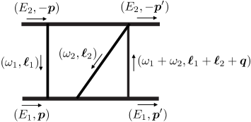
Figure 22: The box-triangle diagram.

Consider next the general box triangle diagram, which is a two-loop integral with an arbitrary numerator and two $\phi_{1}$ propagators, one $\phi_{2}$ propagator, and three graviton propagators as arranged in Fig. 22. The integrand corresponding to this diagram is

$${\cal I}_{{\rm BT}}= \frac{1}{(E_{1}+\omega_{1})^{2}-(\bm{p}+\bm{\ell}_{1})^{2}-m_{1}^{2}}\,\frac{1}{(E_{1}+\omega_{1}+\omega_{2})^{2}-(\bm{p}+\bm{\ell}_{1}+\bm{\ell}_{2})^{2}-m_{1}^{2}}$$ (7.79)

$$\times\frac{1}{(E_{2}-\omega_{1})^{2}-(\bm{p}+\bm{\ell}_{1})^{2}-m_{2}^{2}}\,\frac{1}{\omega_{1}^{2}-\bm{\ell}_{1}^{2}}\,\frac{1}{\omega_{2}^{2}-\bm{\ell}_{2}^{2}}\,\frac{1}{(\omega_{1}+\omega_{2})^{2}-(\bm{\ell}_{1}+\bm{\ell}_{2}+\bm{q})^{2}}\,{\cal N}_{{\rm BT}}\,.$$

We factor all matter propagators into matter and antimatter components,

$$\frac{1}{(E_{1}+\omega_{1})^{2}-(\bm{p}+\bm{\ell}_{1})^{2}-m_{1}^{2}} =\frac{1}{(\omega_{1}-\omega_{P_{1}})(\omega_{1}-\omega_{A_{1}})}\,,$$ (7.80)

$$\frac{1}{(E_{2}-\omega_{1})^{2}-(\bm{p}+\bm{\ell}_{1})^{2}-m_{2}^{2}} =\frac{1}{(\omega_{1}-\omega_{P_{2}})(\omega_{1}-\omega_{A_{2}})}\,,$$

$$\frac{1}{(E_{1}+\omega_{1}+\omega_{2})^{2}-(\bm{p}+\bm{\ell}_{1}+\bm{\ell}_{2})^{2}-m_{1}^{2}} =\frac{1}{(\omega_{1}+\omega_{2}-\omega_{P^{\prime}_{1}})(\omega_{1}+\omega_{2}-\omega_{A^{\prime}_{1}})}\,.$$

The spatial integrand is then given in terms of the effective numerator by

$$\widetilde{\cal I}_{{\rm BT}} =\int\frac{d\omega_{1}}{2\pi}\frac{d\omega_{2}}{2\pi}\,\frac{\widetilde{\cal N}_{{\rm BT}}(\omega_{1},\omega_{2})}{(\omega_{1}-\omega_{P_{1}})(\omega_{1}-\omega_{P_{2}})(\omega_{1}+\omega_{2}-\omega_{P_{1}^{\prime}})}\,,$$ (7.81)

where

$$\widetilde{\cal N}_{{\rm BT}}(\omega_{1},\omega_{2}) =\frac{1}{\omega_{1}-\omega_{A_{1}}}\frac{1}{\omega_{1}-\omega_{A_{2}}}\,\frac{1}{\omega_{1}+\omega_{2}-\omega_{A_{1}^{\prime}}}\,\frac{1}{\omega_{1}^{2}-\bm{\ell}_{1}^{2}}\,\frac{1}{\omega_{2}^{2}-\bm{\ell}_{2}^{2}}\,$$ (7.82)

$$\hskip 113.81102pt\hbox{}\times\frac{1}{(\omega_{1}+\omega_{2})^{2}-(\bm{\ell}_{1}+\bm{\ell}_{2}+\bm{q})^{2}}\,{\cal N}_{{\rm BT}}(\omega_{1},\omega_{2})\,.$$

Next, we implement energy-integral reduction. From the diagram’s topology, we see that the constraints are a combination of those of the one-loop box and triangle integrals:

$$(\omega_{1}-\omega_{P_{1}})(\omega_{1}-\omega_{P_{2}})\rightarrow 0\qquad{\rm and}\qquad\omega_{1}+\omega_{2}-\omega_{P_{1}^{\prime}}\rightarrow 0\,.$$ (7.83)

Hence we can effectively evaluate the numerator

$$\widetilde{\cal N}_{{\rm BT}}(\omega_{1},\omega_{2})\rightarrow\widetilde{\cal N}_{{\rm BT}}(\omega_{1},\omega_{P_{1}^{\prime}}-\omega_{1})\,,$$ (7.84)

and then treat the remaining dependence on $\omega_{1}$ as we would for the one-loop box. That is, we reduce it to a linear function using the first constraint in Eq. (7.83), and then expand about either $\omega_{P_{1}}$ or $\omega_{P_{2}}$. This would cancel one of the factors in $(\omega_{1}-\omega_{P_{1}})(\omega_{1}-\omega_{P_{2}})$ and lead to either the master for the double-triangle diagram in Eq. (7.42) or the master for the double-triangle prime diagram in Eq. (7.54). We of course have terms with all three matter poles uncanceled, and thus the box triangle master energy integral:

$$\int\frac{d\omega_{1}\,d\omega_{2}}{(\omega_{1}-\omega_{P_{1}}+i\epsilon)(\omega_{1}-\omega_{P_{2}}-i\epsilon)(\omega_{1}+\omega_{2}-\omega_{P_{1}^{\prime}}+i\epsilon)}$$ (7.85)

$$\quad\equiv\frac{1}{3!}\left(\int\frac{d\omega_{1}\,d\omega_{2}}{(\omega_{1}-\omega_{P_{1}}+i\epsilon)(\omega_{1}-\omega_{P_{2}}-i\epsilon)(\omega_{1}+\omega_{2}-\omega_{P_{1}^{\prime}}+i\epsilon)}+\{\textrm{perm.}\}\right)$$

$$\quad=\frac{1}{2(\omega_{P_{1}}-\omega_{P_{2}})}\times(-2\pi i)^{2}\,.$$

Consider for illustration the case ${\cal N}_{{\rm BT}}=1$. Upon implementing the above procedure, we obtain the spatial integrand,

$$\widetilde{\cal I}_{{\rm BT}} =-\frac{1}{8E_{1}(E_{2}+E_{1})\bm{\ell}_{1}^{2}(\bm{\ell}_{2}-\bm{\ell}_{1})^{2}(\bm{\ell}_{2}+\bm{q})^{2}(\bm{\ell}_{1}^{2}+2\bm{p}\bm{\ell}_{1})}\bigg{[}1+\frac{(\bm{\ell}_{2}^{2}+2\bm{p}\bm{\ell}_{2})(\bm{\ell}_{1}^{2}+2\bm{p}\bm{\ell}_{1})}{3E_{2}E_{1}(\bm{\ell}_{2}-\bm{\ell}_{1})^{2}}$$ (7.86)

$$\quad-\frac{(\bm{\ell}_{2}^{2}+2\bm{p}\bm{\ell}_{2})(\bm{\ell}_{1}^{2}+2\bm{p}\bm{\ell}_{1})}{6E_{1}^{2}(\bm{\ell}_{2}-\bm{\ell}_{1})^{2}}+\frac{(\bm{\ell}_{2}^{2}+2\bm{p}\bm{\ell}_{2})^{2}}{4E_{1}^{2}(\bm{\ell}_{2}+\bm{q})^{2}}+\frac{(\bm{\ell}_{2}^{2}+2\bm{p}\bm{\ell}_{2})^{2}}{4E_{1}^{2}(\bm{\ell}_{2}-\bm{\ell}_{1})^{2}}-\frac{(\bm{\ell}_{2}^{2}+2\bm{p}\bm{\ell}_{2})}{2E_{1}^{2}}+\frac{(\bm{\ell}_{1}^{2}+2\bm{p}\bm{\ell}_{1})^{2}}{6E_{2}^{2}(\bm{\ell}_{2}-\bm{\ell}_{1})^{2}}$$

$$\quad+\frac{(\bm{\ell}_{1}^{2}+2\bm{p}\bm{\ell}_{1})^{2}}{12E_{1}^{2}(\bm{\ell}_{2}-\bm{\ell}_{1})^{2}}+\frac{(\bm{\ell}_{1}^{2}+2\bm{p}\bm{\ell}_{1})^{2}}{6E_{2}^{2}\bm{\ell}_{1}^{2}}+\frac{(\bm{\ell}_{1}^{2}+2\bm{p}\bm{\ell}_{1})^{2}}{12E_{1}^{2}\bm{\ell}_{1}^{2}}-\frac{(\bm{\ell}_{1}^{2}+2\bm{p}\bm{\ell}_{1})}{6E_{2}^{2}}-\frac{(\bm{\ell}_{1}^{2}+2\bm{p}\bm{\ell}_{1})}{12E_{1}^{2}}+\cdots\bigg{]}\,,$$

where we have shifted the integration variable $\bm{\ell}_{2}\to\bm{\ell}_{2}-\bm{\ell}_{1}$, and the ellipsis denotes higher-order terms in the nonrelativistic expansion. Applying Eq. (7.9) sequentially to each integral, we obtain,

$$I_{{\rm BT}} =-\frac{1}{64E_{1}E}\int\frac{d^{D-1}\bm{\ell}_{1}}{(2\pi)^{D-1}}\frac{1}{\bm{\ell}_{1}^{2}|\bm{\ell}_{1}-\bm{q}|(\bm{\ell}_{1}^{2}+2\bm{p}\bm{\ell}_{1})}\left[1+\frac{\bm{p}^{2}}{2E_{1}^{2}}+\frac{3\bm{p}^{4}}{8E_{1}^{4}}+\frac{5\bm{p}^{6}}{16E_{1}^{6}}+\frac{35\bm{p}^{8}}{128E_{1}^{8}}+\cdots\right]$$ (7.87)

$$\quad+{\ln{\bm{q}}^{2}\over 2048\pi^{2}E_{1}^{3}E}\bigg{[}1+{5\bm{p}^{2}\over 4E_{1}^{2}}+{11\bm{p}^{4}\over 8E_{1}^{4}}+{93\bm{p}^{6}\over 64E_{1}^{6}}+\cdots\bigg{]}\,,$$

where we have included results for higher-order terms not shown explicitly in Eq. (7.86). Resummation of the series (see Appendix C for details) yields

$$I_{{\rm BT}} =-\frac{1}{64m_{1}E}\int\frac{d^{D-1}\bm{\ell}_{1}}{(2\pi)^{D-1}}\frac{1}{\bm{\ell}_{1}^{2}|\bm{\ell}_{1}-\bm{q}|(\bm{\ell}_{1}^{2}+2\bm{p}\bm{\ell}_{1})}+{\ln{\bm{q}}^{2}(E_{1}-m_{1})\over 1024\pi^{2}m_{1}^{2}E\bm{p}^{2}}\,,$$ (7.88)

where the second term is the classical contribution. The remaining integral has the form of Eq. (7.8) with $\gamma=1$. It is superclassical, having an additional factor of $|\bm{q}|^{-1}$ relative to the classical scaling, and represents the iteration of the lower-order tree-level and one-loop triangle diagrams. It is infrared divergent and will cancel with the same infrared artifact appearing in the effective-theory contribution to the matching.

7.3.5 Double-Box Diagram

Consider the general double-box diagram which is a two-loop integral with an arbitrary numerator and two $\phi_{1}$ propagators, two $\phi_{2}$ propagators, and three graviton propagators arranged as in Fig. 23.

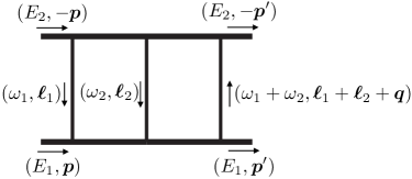
Figure 23: The double-box diagram.

The integrand corresponding to this diagram is

$${\cal I}_{{\rm BB}}= \frac{1}{(E_{1}+\omega_{1})^{2}-(\bm{p}+\bm{\ell}_{1})^{2}-m_{1}^{2}}\,\frac{1}{(E_{2}-\omega_{1})^{2}-(\bm{p}+\bm{\ell}_{1})^{2}-m_{2}^{2}}$$ (7.89)

$$\times\frac{1}{(E_{1}+\omega_{1}+\omega_{2})^{2}-(\bm{p}+\bm{\ell}_{1}+\bm{\ell}_{2})^{2}-m_{1}^{2}}\,\frac{1}{(E_{2}-\omega_{1}-\omega_{2})^{2}-(\bm{p}+\bm{\ell}_{1}+\bm{\ell}_{2})^{2}-m_{2}^{2}}$$

$$\times\frac{1}{\omega_{1}^{2}-\bm{\ell}_{1}^{2}}\,\frac{1}{\omega_{2}^{2}-\bm{\ell}_{2}^{2}}\,\frac{1}{(\omega_{1}+\omega_{2})^{2}-(\bm{\ell}_{1}+\bm{\ell}_{2}+\bm{q})^{2}}\,{\cal N}_{{\rm BB}}\,.$$

As before, we factor all propagators into matter and antimatter components. The spatial integrand is then given in terms of the effective numerator by

$$\widetilde{\cal I}_{{\rm BB}} =\int\frac{d\omega_{1}}{2\pi}\frac{d\omega_{2}}{2\pi}\,\frac{\widetilde{\cal N}_{{\rm BB}}(\omega_{1},\omega_{2})}{(\omega_{1}-\omega_{P_{1}})(\omega_{1}-\omega_{P_{2}})(\omega_{1}+\omega_{2}-\omega_{P_{1}^{\prime}})(\omega_{1}+\omega_{2}-\omega_{P_{2}^{\prime}})}\,,$$ (7.90)

where

$$\widetilde{\cal N}_{{\rm BB}}(\omega_{1},\omega_{2}) =\frac{1}{\omega_{1}-\omega_{A_{1}}}\frac{1}{\omega_{1}-\omega_{A_{2}}}\,\frac{1}{\omega_{1}+\omega_{2}-\omega_{A_{1}^{\prime}}}\,\frac{1}{\omega_{1}+\omega_{2}-\omega_{A_{2}^{\prime}}}\,\frac{1}{\omega_{1}^{2}-\bm{\ell}_{1}^{2}}\,\frac{1}{\omega_{2}^{2}-\bm{\ell}_{2}^{2}}$$ (7.91)

$$\qquad\times\frac{1}{(\omega_{1}+\omega_{2})^{2}-(\bm{\ell}_{1}+\bm{\ell}_{2}+\bm{q})^{2}}\,{\cal N}_{{\rm BB}}(\omega_{1},\omega_{2})\,.$$

The energy-reduction constraints take the form

$$(\omega_{1}-\omega_{P_{1}})(\omega_{1}-\omega_{P_{2}}) \rightarrow 0\,,$$ (7.92)

$$(\omega_{1}+\omega_{2}-\omega_{P_{1}^{\prime}})(\omega_{1}+\omega_{2}-\omega_{P_{2}^{\prime}}) \rightarrow 0\,.$$

These constraints reduce the effective numerator to the form

$${\cal N}_{{\rm BB}}(\omega_{1},\omega_{2})=f_{0}+f_{1}\omega_{1}+f_{2}\omega_{2}+f_{3}\omega_{1}\omega_{2}\,.$$ (7.93)

As before, the remaining dependence on $\omega_{1}$ and $\omega_{2}$ can be expanded about a chosen energy pole, leading to the previously encountered energy master integrals for the box-triangle, double-triangle, and double-triangle prime diagrams. The term independent of $\omega_{1}$ and $\omega_{2}$ require the double-box master integral given by

$$\int\frac{d\omega_{1}\,d\omega_{2}}{(\omega_{1}-\omega_{P_{1}}+i\epsilon)(\omega_{1}-\omega_{P_{2}}-i\epsilon)(\omega_{1}+\omega_{2}-\omega_{P_{1}^{\prime}}+i\epsilon)(\omega_{1}+\omega_{2}-\omega_{P_{2}^{\prime}}-i\epsilon)}$$ (7.94)

$$=\frac{1}{(\omega_{P_{1}}-\omega_{P_{2}})(\omega_{P_{1}^{\prime}}-\omega_{P_{2}^{\prime}})}\times(-2\pi i)^{2}\,.$$

As before, consider for illustration the case ${\cal N}_{{\rm BB}}=1$. Upon expanding in the classical and nonrelativistic limits, we obtain the spatial integrand

$$\widetilde{\cal I}_{{\rm BB}} =\frac{1}{4E^{2}\bm{\ell}_{1}^{2}(\bm{\ell}_{2}-\bm{\ell}_{1})^{2}(\bm{\ell}_{2}+\bm{q})^{2}(\bm{\ell}_{1}^{2}+2\bm{p}\bm{\ell}_{1})(\bm{\ell}_{2}^{2}+2\bm{p}\bm{\ell}_{2})}+\cdots\,,$$ (7.95)

where we have shifted the integration variable $\bm{\ell}_{2}\to\bm{\ell}_{2}-\bm{\ell}_{1}$, and the ellipsis denotes higher-order terms in the nonrelativistic expansion. Applying Eq. (7.9) sequentially to each integral, we obtain,

$$I_{{\rm BB}} =\frac{1}{4E^{2}}\int\frac{d^{D-1}\bm{\ell}_{1}}{(2\pi)^{D-1}}\frac{d^{D-1}\bm{\ell}_{2}}{(2\pi)^{D-1}}\frac{1}{\bm{\ell}_{1}^{2}(\bm{\ell}_{2}-\bm{\ell}_{1})^{2}(\bm{\ell}_{2}+\bm{q})^{2}(\bm{\ell}_{1}^{2}+2\bm{p}\bm{\ell}_{1})(\bm{\ell}_{2}^{2}+2\bm{p}\bm{\ell}_{2})}\,.$$ (7.96)

The remaining integral here is infrared divergent and superclassical, having an additional factor of $|\bm{q}|^{-2}$ relative to the classical scaling. It represents the iteration of the lower-order tree-level diagram, and we will leave the integral unevaluated since it will simply cancel with the same infrared artifact appearing in the effective theory contribution to the matching. As in the case of the one-loop box diagram, the classical contributions vanish order by order in the nonrelativistic expansion.

7.3.6 Crossed-Double-Box Diagram

Finally we consider the general nonplanar double-box diagram, which is a two-loop nonplanar integral with an arbitrary numerator and two $\phi_{1}$ propagators, two $\phi_{2}$ propagators, and three graviton propagators arranged as shown in Fig. 24.

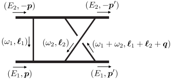
Figure 24: The nonplanar double-box diagram.

The integrand corresponding to this diagram is

$${\cal I}_{{\rm B}\overline{\rm B}}= \frac{1}{(E_{1}+\omega_{1})^{2}-(\bm{p}+\bm{\ell}_{1})^{2}-m_{1}^{2}}\,\frac{1}{(E_{2}-\omega_{1})^{2}-(\bm{p}+\bm{\ell}_{1})^{2}-m_{2}^{2}}$$ (7.97)

$$\times\frac{1}{(E_{1}+\omega_{1}+\omega_{2})^{2}-(\bm{p}+\bm{\ell}_{1}+\bm{\ell}_{2})^{2}-m_{1}^{2}}\frac{1}{(E_{2}+\omega_{2})^{2}-(\bm{p}-\bm{\ell}_{2}-\bm{q})^{2}-m_{2}^{2}}\,\frac{1}{\omega_{1}^{2}-\bm{\ell}_{1}^{2}}\,$$

$$\times\frac{1}{\omega_{2}^{2}-\bm{\ell}_{2}^{2}}\,\frac{1}{(\omega_{1}+\omega_{2})^{2}-(\bm{\ell}_{1}+\bm{\ell}_{2}+\bm{q})^{2}}\,{\cal N}_{{\rm B}\overline{\rm B}}\,.$$

As before, we factor all propagators into matter and antimatter components. The spatial integrand is then

$$\widetilde{\cal I}_{{\rm B}\overline{\rm B}} =\int\frac{d\omega_{1}}{2\pi}\frac{d\omega_{2}}{2\pi}\,\frac{\widetilde{\cal N}_{{\rm B}\overline{\rm B}}(\omega_{1},\omega_{2})}{(\omega_{1}-\omega_{P_{1}})(\omega_{1}-\omega_{P_{2}})(\omega_{1}+\omega_{2}-\omega_{P_{1}^{\prime}})(\omega_{2}-\omega_{P_{2}^{\prime}})}\,,$$ (7.98)

where the effective numerator is

$$\widetilde{\cal N}_{{\rm B}\overline{\rm B}}(\omega_{1},\omega_{2}) =\frac{1}{\omega_{1}-\omega_{A_{1}}}\frac{1}{\omega_{1}-\omega_{A_{2}}}\,\frac{1}{\omega_{1}+\omega_{2}-\omega_{A_{1}^{\prime}}}\,\frac{1}{\omega_{2}-\omega_{A_{2}^{\prime}}}\,\frac{1}{\omega_{1}^{2}-\bm{\ell}_{1}^{2}}\,\frac{1}{\omega_{2}^{2}-\bm{\ell}_{2}^{2}}$$ (7.99)

$$\quad\times\frac{1}{(\omega_{1}+\omega_{2})^{2}-(\bm{\ell}_{1}+\bm{\ell}_{2}+\bm{q})^{2}}\,{\cal N}_{{\rm B}\overline{\rm B}}(\omega_{1},\omega_{2})\,.$$

The energy-reduction constraints take the form

$$(\omega_{1}-\omega_{P_{1}})(\omega_{1}-\omega_{P_{2}})(\omega_{1}+\omega_{2}-\omega_{P_{1}^{\prime}}) \rightarrow 0\,,$$ (7.100)

$$(\omega_{1}-\omega_{P_{1}})(\omega_{1}-\omega_{P_{2}})(\omega_{2}-\omega_{P_{2}^{\prime}}) \rightarrow 0\,,$$

$$(\omega_{1}+\omega_{2}-\omega_{P_{1}^{\prime}})(\omega_{2}-\omega_{P_{2}^{\prime}}) \rightarrow 0\,.$$

We can solve for $\omega_{1}^{3}$ from the first constraint, $\omega_{1}^{2}$ from the second constraint, and $\omega_{2}^{2}$ from the third constraint. This allows us to reduce the effective numerator to the form

$${\cal N}_{{\rm B}\overline{\rm B}}(\omega_{1},\omega_{2})=f_{0}+f_{1}\omega_{1}+f_{2}\omega_{2}+f_{3}\omega_{1}\omega_{2}\,.$$ (7.101)

As before, the remaining dependence on $\omega_{1}$ and $\omega_{2}$ can be expanded about a chosen energy pole. In particular the last two terms in Eq. (7.101) lead to the previously encountered energy master integrals for the box-triangle, double-triangle, and double-triangle prime diagrams. The first and second terms lead to vanishing masters given by

$$\int\frac{d\omega_{1}\,d\omega_{2}}{(\omega_{1}-\omega_{P_{1}}+i\epsilon)(\omega_{1}-\omega_{P_{2}}-i\epsilon)(\omega_{1}+\omega_{2}-\omega_{P_{1}^{\prime}}+i\epsilon)(\omega_{2}-\omega_{P_{2}^{\prime}}+i\epsilon)} =0\,,$$ (7.102)

$$\int\frac{d\omega_{1}\,d\omega_{2}}{(\omega_{1}-\omega_{P_{1}}+i\epsilon)(\omega_{1}+\omega_{2}-\omega_{P_{1}^{\prime}}+i\epsilon)(\omega_{2}-\omega_{P_{2}^{\prime}}+i\epsilon)} =0\,.$$

These were evaluated by averaging over six permutations of the three exchanged gravitons.

As in the case of the one-loop scalar crossed box, the two-loop crossed-double-box with ${\cal N}_{{\rm B}\overline{\rm B}}=1$ vanishes order by order in the velocity expansion.

7.4 Quantum Contributions

In the previous subsections we have described various diagrams which contribute to classical scattering. Conversely, we have dropped many contributions which, as discussed in Sec. 2.3, would otherwise contribute to the scattering amplitude but are quantum mechanical. Restricting to the classical contribution to the conservative potential, we then restrict consideration to diagrams in which

• every loop includes at least one matter propagator,

• there are no gravitons starting and ending at the same matter line.

These would exclude, for example, the diagrams shown in Fig. 25, where diagrams (a) and (b) respectively violate the first and second criteria.

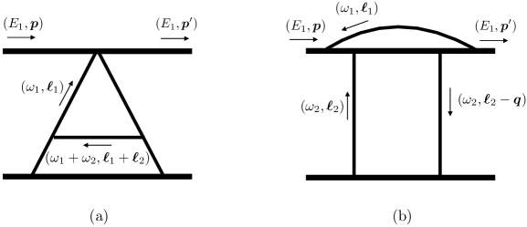
Figure 25: Examples of diagrams that do not have classical potential contributions.

We discuss here the above criteria in terms of the mechanics of the nonrelativistic method of integration described in this section. Consider an internal graviton line with momentum $(\omega,\bm{\ell})$. The component $\omega$ is set through energy integration to a matter pole, e.g. $\omega_{P_{1}}$, which at leading order goes as $\omega_{P_{1}}\sim{\bm{p}\cdot\bm{\ell}/m_{1}}$. At the same time, as seen from Eq. (7.8) the component $\bm{\ell}$ is set by a graviton pole in $(D-1)$-momentum variables to be of order the momentum transfer, $|\bm{\ell}|\sim|\bm{q}|$. These, of course, are consistent with the potential region, where a graviton loop momentum goes as $(\omega,\bm{\ell})\sim(|\bm{v}||\bm{q}|,|\bm{q}|)$. However, the energy or $(D-1)$-momentum components cannot be of the same order as the scales $m$ or $|\bm{p}|$ while being in the potential region. There is also the radiation region but, as discussed in Sec. 12.3, this only affects emission, at least at the order at which we are computing.

From these remarks the criteria above are straightforward to understand. The first criterion is necessary because the energy flowing through a loop that does not include a matter propagator cannot be set to the matter pole, and is therefore not in the potential region. For example, consider the dependence on the graviton loop momentum $(\omega_{1},\bm{\ell}_{1})$ in diagram (a) in Fig. 25. The loop energy $\omega_{1}$ has no pole in $\omega_{P_{1}}$ because there is no matter propagator for $\phi_{1}$. Note that the middle horizontal graviton depends on the sum $\omega_{1}+\omega_{2}$ but this is subleading to the $(D-1)$-momentum component since it is a potential mode, and does not correspond to a pole for $\omega_{1}$. This diagram fails the first criterion. On the other hand, this diagram has a pole in $\bm{\ell}_{1}-\bm{q}$ and passes the second criterion.

The second criterion is necessary because the momentum flowing through a graviton starting and ending on the same matter line cannot have a scale set to the momentum transfer. As a concrete example, consider the dependence on the graviton loop momentum $(\omega_{1},\bm{\ell}_{1})$ in diagram (b) in Fig. 25. The loop energy $\omega_{1}$ can be set to a matter pole since there are matter propagators for $\phi_{1}$. However, there is no pole in $\bm{\ell}_{1}-\bm{q}$. Note that the matter propagators for $\phi_{1}$ depend on the spatial momenta $\bm{p}$, $\bm{\ell}_{2}$, and $\bm{q}$, but there is no pole in $\bm{\ell}_{1}-\bm{q}$ or $\bm{\ell}_{1}-\bm{\ell}_{2}$.

7.5 Residue Method

In this section we discuss an alternative simpler method for performing the energy integration. In the previous examples our approach was to apply energy-integral reduction to express everything in terms of master energy integrals which were then evaluated directly. Here we will see that we can instead evaluate the energy integrals using residues. This has been verified explicitly at two loops.

Recall that the spatial integrand $\widetilde{\cal I}$ is equal to the energy integral of the full integrand,

$$\widetilde{\cal I}=\bigg{[}\prod_{i=1}^{n_{L}}\int\frac{d\omega_{i}}{2\pi}\bigg{]}\;{\cal I}\,.$$ (7.103)

In general, ${\cal I}$ will have singularities from graviton poles as well as matter and antimatter poles. Of course, only the matter poles reside in the kinematic region which contributes classically. In general, we can take the $n_{L}$ loop energies and localize them onto $n_{L}$ of the $n_{M}$ matter poles. We label each of these solutions $\omega_{i\alpha}$ by an index $\alpha$. Our claim is that the energy integral is equal to

$$\widetilde{\cal I}=\sum_{\alpha}\sigma_{\alpha}\!\!\underset{\;\;\;\omega_{i}=\omega_{i\alpha}}{\rm Res}[{\cal I}]\,,$$ (7.104)

where $\sigma_{\alpha}$ is a numerical symmetry factor associated with each residue. To determine $\sigma_{\alpha}$ we interpret the residue as cutting certain matter propagators, while all uncut matter propagators should be thought of as pinched. The resulting diagram then corresponds to one of the master energy integrals we have considered already, and $\sigma_{\alpha}$ is precisely the associated symmetry factor.

The residue method can be derived from the method of energy integral reduction. Consider expanding the integrand ${\cal I}$, written as Eq. (7.5), in the potential region. Then the effective numerator $\widetilde{\cal N}$ is a power series in $\omega_{i}$. The power series can be organized into terms that pinch all energy poles, and terms with singularities in $\omega_{i}$. The first type integrates to zero via Eq. (7.6). This is trivially equivalent to taking the residue because the corresponding energy integrand is regular in the finite region. The second type are nothing but the energy master integrals, e.g. Eq. (7.29) and Eq. (7.42), and evaluate to residues with appropriate symmetry factors. Hence, the energy integration for each term in the expansion of $\widetilde{\cal N}$ is equivalent to taking the residue and including symmetry factors, and therefore the answer should reproduce Eq. (7.104) after expanding in the potential region.

We briefly discuss how this works in some of our earlier examples in Sec. 7.2 and 7.3. First, we consider one loop, where $\omega_{i}$ runs over a single loop energy. The triangle diagram has one matter pole so $\alpha$ runs over one solution. As we have shown the associated symmetry factor is $\sigma_{\alpha}=\{1/2\}$. Meanwhile, for both the box and crossed-box diagrams there are two matter poles so $\alpha$ runs over two solutions with symmetry factors $\sigma_{\alpha}=\{1/2,1/2\}$.

Moving on to two loops, we see that the double-triangle diagram has two matter poles. Since $\omega_{i}$ runs over two-loop energies, $\alpha$ runs over a single solution for which $\sigma_{\alpha}=\{1/6\}$. The box-triangle diagram is more complicated because it has three matter poles. A priori, there are three ways to localize two-loop energies onto these matter poles. However, one of these configurations does not exist because there is no choice of loop energy that can localize both matter poles residing in a box subdiagram. Consequently, for the box-triangle diagram, $\alpha$ runs over two solutions with symmetry factors $\sigma_{\alpha}=\{1/6,1/3\}$, which is consistent with the energy master integral in Eq. (7.85) since $1/3+1/6=1/2$.

8 Relativistic Integration

Ideally, we would evaluate all integrals via fully relativistic methods. As we will see, this is relatively straightforward for certain diagrams—in particular, those which are free from infrared divergent matter singularities. One notable example is the H and crossed-H diagrams in Sec. 7.3.3, whose resummation yielded the arcsinh function. In the present section, we describe several relativistic methods, such as differential equations and Mellin-Barnes integration, for analytic computation of the H diagram and other integrals in the same class, including the diagram in Sec. 7.3.2. These methods provides strong confirmation that we have indeed correctly resummed the amplitude to all orders in velocity.

8.1 Method of Differential Equations

Differential equations are a powerful method for evaluating Feynman integrals Kotikov:1990kg ; hep-ph/9306240 ; hep-th/9711188 ; GehrmannRemiddi . We will adapt the method to evaluate the classical contribution of the sum of the H and $\overline{\rm H}$ integrals, using differential equations for integrals localized on the poles of the two internal matter lines.

The class of integrals we will discuss, denoted by ${\rm H}[a_{1}\dots a_{9}]$, is defined as

$${\rm H}[a_{1},\dots a_{7},a_{8},a_{9}]=\int\frac{d^{D}\ell_{1}d^{D}\ell_{4}}{(2\pi)^{2D}}\frac{((\ell_{4}+p_{1})^{2}-m_{1}^{2})^{-a_{8}}((\ell_{1}-p_{2})^{2}-m_{2}^{2})^{-a_{9}}}{(\ell_{1}^{2})^{a_{1}}(\ell_{2}^{2}-m_{1}^{2})^{a_{2}}(\ell_{3}^{2})^{a_{3}}(\ell_{4}^{2})^{a_{4}}(\ell_{5}^{2}-m_{2}^{2})^{a_{5}}(\ell_{6}^{2})^{a_{6}}(\ell_{7}^{2})^{a_{7}}}\,,$$ (8.1)

with the momentum labeling in Fig. 26 and $\ell_{2,3,5,6,7}$ expressed in terms of $\ell_{1}$ and $\ell_{4}$ by momentum conservation.

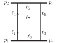
Figure 26: The H graph with momentum assignments. The 7 propagators carrying momentum $\ell_{i}$ correspond to the propagators in Eq. (8.1). The external momenta are all outgoing and the direction of the independent loop momenta are indicated by the arrows.

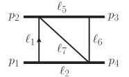
Figure 27: The diagram ${\rm H}[1,1,0,0,1,1,1,0,0]$, with momentum assignments, obtained by canceling propagators 3 and 4 of the H diagram in Fig. 26.

8.1.1 Integration-By-Parts Reduction

To obtain differential equations, we first perform integration-by-parts (IBP) reduction Chetyrkin:1981qh ; Laporta:2001dd in $D=4-2\epsilon$ dimensions. There are by now many automated IBP reduction programs. We use Kira Maierhoefer:2017hyi which implements fast modern algorithms. All integrals of the H diagram and a tower of contact diagrams with collapsed propagators are reduced to $51$ master integrals.

The most important master integrals are associated with the H diagram, ${\rm H}[1,1,1,1,1,1,1,0,0]$, and with ${\rm H}[1,1,0,0,1,1,1,0,0]$. It turns out that diagrams ${\rm H}[0,1,1,1,1,1,1,0,0]$, ${\rm H}[1,1,0,1,1,1,1,0,0]$, ${\rm H}[1,1,1,0,1,1,1,0,0]$ or ${\rm H}[1,1,1,1,1,0,1,0,0]$, obtained from H by canceling one of the propagators 1, 3, 4, or 6 respectively, have no master integrals. That is, all integrals ${\rm H}[a_{1},1,1,1,1,1,1,a_{8},a_{9}]$, ${\rm H}[1,1,a_{3},1,1,1,1,a_{8},a_{9}]$, ${\rm H}[1,1,1,a_{4},1,1,1,a_{8},a_{9}]$ or ${\rm H}[1,1,1,1,1,a_{6},1,a_{8},a_{9}]$ with $a_{1,3,4,6,8,9}\leq 0$, can be reduced (via IBP) to master integrals of the diagram ${\rm H}[1,1,0,0,1,1,1,0,0]$.

The master integrals associated with the H graph in Fig. 26, i.e. the integrals that can be used to express any integral of the type ${\rm H}[1,1,1,1,1,1,1,a_{8},a_{9}]$ with $a_{8,9}\leq 0$ modulo contact integrals with fewer propagators, are (rescaled by appropriate powers of $t=-{\bm{q}}^{2}$ to have classical power counting)

$$I_{1}=t^{2}\,{\rm H}[1,1,1,1,1,1,1,0,0]\,,\hskip 54.06006ptI_{2}=t^{3/2}\,{\rm H}[1,1,1,1,1,1,1,0,-1]\,,$$

$$I_{3}=t^{3/2}\,{\rm H}[1,1,1,1,1,1,1,-1,0]\,,\hskip 36.98866ptI_{4}=t\,{\rm H}[1,1,1,1,1,1,1,-2,0]\,.$$ (8.2)

The master integrals associated with the graph ${\rm H}[1,1,0,0,1,1,1,0,0]$ in Fig. 27, i.e. the integrals that can be used to express any integral of the type ${\rm H}[1,1,a_{3},a_{4},1,1,1,a_{8},a_{9}]$ with $a_{3,4,8,9}\leq 0$ modulo contact integrals with fewer propagators, are

$$I_{5}={\rm H}[1,1,0,0,1,1,1,0,0]\,,\hskip 71.13188ptI_{6}=t^{-1/2}\,{\rm H}[1,1,0,0,1,1,1,0,-1]\,,$$

$$I_{7}=t^{-1/2}\,{\rm H}[1,1,0,0,1,1,1,-1,0]\,,\hskip 36.98866ptI_{8}=t^{-1}\,{\rm H}[1,1,-1,0,1,1,1,0,0]\,,$$

$$I_{9}=t^{-2}\,{\rm H}[1,1,-2,0,1,1,1,0,0]\,.$$ (8.3)

We omit the expressions for the remaining master integrals. In fact, they are associated with diagram topologies that cannot give rise to a classical $1/r^{3}$ potential; among them are topologies with collapsed matter propagators and topologies with four-scalar contact vertices. This also matches the construction of the integrand in Sec. 6.4, where the two internal matter lines in graphs of H topology are always cut and therefore never collapsed.

8.1.2 Differential Equations

The derivative of a master integral with respect to any kinematic variable, such as $(\partial/\partial\sigma)$, can be rewritten in the form

$$\Omega_{ij}\,k_{i}^{\mu}\frac{\partial}{\partial k_{j}^{\mu}}$$ (8.4)

which can then act on the propagators and numerators of an integral. Here $\Omega_{ij}$ is a linear combination of the $GL(3)$ generators. The action of the operator (8.4) generally introduces propagators raised to higher powers, but the IBP reduction re-expresses the result as a linear combination of the original master integrals. Therefore we obtain differential equations GehrmannRemiddi

$$\frac{\partial}{\partial\sigma}\Bigg{|}_{t,\,m_{1}^{2},\,m_{2}^{2}}I_{i}=M_{ij}\,I_{j},$$ (8.5)

with some matrix $M_{ij}$ whose entries are rational functions of the kinematic variables $\sigma=(p_{1}\cdot p_{2})/(m_{1}m_{2}),t=-{\bm{q}}^{2},m_{1}^{2},m_{2}^{2}$.

We define the “conjugate” master integrals from a $s\leftrightarrow u$ crossing,

$$\bar{I}_{i}=I_{i}|_{p_{2}\leftrightarrow p_{3}},\quad i=1,2,\dots,9$$ (8.6)

As shown in Section 7, in the small-$t$ limit, the conservative contribution from the sum,

$$\hat{I}_{i}=\operatorname{Re}(I_{i}+\bar{I}_{i})\,,$$ (8.7)

is effectively a modified version of $I_{i}$ with the two matter propagators replaced by delta functions, see Sec. 8.2. By dropping master integrals with collapsed matter propagators, and taking the small-$t$ limits of the $M_{ij}$ entries in Eq. (8.5), we obtain the final differential equations that are valid for integrals localized on the matter poles, similar to the energy integration procedure,

$$\frac{\partial}{\partial\sigma}\Bigg{|}_{t,\,m_{1}^{2},\,m_{2}^{2}}\hat{I}_{i}={\widetilde{M}}_{ij}\,\hat{I}_{j},$$ (8.8)

where the values of $i$ and $j$ only run from $1$ to $9$, corresponding to the 9 master integrals in Eqs. (8.2) and (8.3), and the matrix $\widetilde{M}$ on the right-hand side is defined as

$$\widetilde{M}_{ij}=M_{ij}|_{t=0}\,.$$ (8.9)

The limit on the right-hand side is well-defined because the $M_{ij}$ entries are all non-singular at $t=0$, thanks to the appropriate normalizations by powers of $t$ in Eqs. (8.2) and (8.3).

To solve the differential equations Eq. (8.8), the boundary condition is that all the integrals are non-singular in the threshold limit, $s\to(m_{1}+m_{2})^{2}$. This is sufficient to fix the solutions up to an overall numerical prefactor. Since the differential equations are homogeneous, the overall prefactor can be fixed by evaluating one integral (in this case, the sum of the scalar H and ${\overline{\rm H}}$ integrals) in the static limit $|\bm{p}|=0$, which is the first term in Eq. (7.77).

The result for $\hat{I}_{1}$, the sum of scalar H and ${\overline{\rm H}}$ integrals localized on matter poles and rescaled by $t^{2}$ as in Eq. (8.2), is equal to

$$\hat{I}_{1}=\frac{\ln\bm{q}^{2}}{64\pi^{2}m_{1}m_{2}}\frac{1}{\sqrt{\sigma^{2}-1}}\operatorname{arcsinh}\sqrt{\frac{\sigma-1}{2}},$$ (8.10)

where $\sigma$ is defined as in Eq. (7.59). We have omitted $\mathcal{O}(\epsilon)$ corrections, as is the case for all results presented in this subsection. The result is in agreement with Eq. (7.78), but is rigorously established by the differential equations to all orders in the velocity expansion. Using hyperbolic trigonometry identities, Eq. (8.10) can be re-written as

$$\hat{I}_{1}=\frac{\ln\bm{q}^{2}}{128\pi^{2}}\,\frac{{\rm arcsinh}(|{\bm{p}}|/m_{1})+{\rm arcsinh}(|{\bm{p}}|/m_{2})}{|{\bm{p}}|(E_{1}+E_{2})},$$ (8.11)

where ${\bm{p}}$, $E_{1}$ and $E_{2}$ are defined in the center-of-mass frame as

$$-p_{1}=(E_{1},{\bm{p}}),\qquad-p_{2}=(E_{2},-{\bm{p}})\,.$$ (8.12)

All other master integrals for the H diagram, combined with the conjugate integrals, have no contribution in the classical limit,

$$\hat{I}_{i}=0,\quad i=2,3,4,5\,.$$ (8.13)

The results for the nonzero master integrals of the diagram ${\rm H}[1,1,0,0,1,1,1,0,0]$, combined with their conjugate integrals, are as follows:

$$\hat{I}_{5} =-\ln{\bm{q}}^{2}\,\frac{1}{128\pi^{2}m_{1}m_{2}}\frac{1}{\sqrt{\sigma^{2}-1}}\operatorname{arcsinh}\sqrt{\frac{\sigma-1}{2}},$$

$$\hat{I}_{8} =\ln{\bm{q}}^{2}\,\frac{\sigma}{256\pi^{2}m_{1}m_{2}}\left(\frac{1}{\sigma^{2}-1}-\frac{2\sigma}{(\sigma^{2}-1)^{3/2}}\operatorname{arcsinh}\sqrt{\frac{\sigma-1}{2}}\right),$$

$$\hat{I}_{9} =\ln{\bm{q}}^{2}\,\frac{(1+2\sigma^{2})}{1024\pi^{2}m_{1}m_{2}(\sigma^{2}-1)^{5/2}}\left(3\sigma\sqrt{\sigma^{2}-1}-2(1+2\sigma^{2})\right)\operatorname{arcsinh}\sqrt{\frac{\sigma-1}{2}}\,.$$ (8.14)

The result for $\hat{I}_{5}$ agrees with the sum of Eq. (7.58) and Eq. (7.60). The other two master integrals of the diagram ${\rm H}[1,1,0,0,1,1,1,0,0]$ vanish in the classical limit when localized on the matter poles,

$$\hat{I}_{j}=0,\quad j=6,7\,.$$ (8.15)

We emphasize that the differential equation method discussed here establishes in a rigorous way that the resummation of the velocity expansion in Eq. (7.77) gives the complete result for the diagram H localized on the matter poles, which is the only part of this diagram that contributes to the conservative potential.

8.1.3 Sample Differential Equations for the Diagram ${\rm H}[1,1,0,0,1,1,1,0,0]$

As a simple illustration, we give sample differential equations for the integrals $\hat{I}_{5,8,9}$ associated with the double triangle prime diagram, ${\rm H}[1,1,0,0,1,1,1,0,0]$ in Fig. 27, in the equal-mass case $m_{1}=m_{2}=1$. In the limit $t\to 0,\,D\to 4$, these integrals are decoupled from the other master integrals in the differential equations,

$$\frac{\partial}{\partial\sigma}\Bigg{|}_{t,\,m_{1}^{2},\,m_{2}^{2}}\hat{I}_{i}=\widetilde{M}_{ij}\,\hat{I}_{j},$$ (8.16)

where the indices $i$ and $j$ take the values $5,8,9$. Setting $t=0,\,D=4,\,m_{1}=m_{2}=1$, the entries of the matrix $\widetilde{M}$ are

$$\widetilde{M}_{5,5} =\frac{2\sigma^{2}+1}{(\sigma-1)\sigma(\sigma+1)},\hskip 25.6073pt\widetilde{M}_{5,8}=-\frac{3\sigma}{(\sigma-1)(\sigma+1)},\hskip 25.6073pt\widetilde{M}_{5,9}=\frac{4}{3\sigma},$$

$$\widetilde{M}_{8,5} =\frac{1}{3\sigma},\hskip 93.89418pt\widetilde{M}_{8,8}=0,\hskip 105.2751pt\widetilde{M}_{8,9}=-\frac{4}{3\sigma},$$

$$\widetilde{M}_{9,5} =-\frac{1}{3\sigma},\hskip 85.35826pt\widetilde{M}_{9,8}=\frac{3\sigma}{(\sigma-1)(\sigma+1)},\hskip 34.14322pt\widetilde{M}_{9,9}=-\frac{11\sigma^{2}+4}{3(\sigma-1)\sigma(\sigma+1)}\,.$$ (8.17)

It can be readily checked that Eq. (8.14) solves the differential equations given above.

The differential equations in $D=4$ are sufficient to determine the master integrals of the diagram ${\rm H}[1,1,0,0,1,1,1,0,0]$ localized on matter poles in the leading small-$t$ limit. In general however we need to keep dependence on $D$, for several reasons. First, the differential equations for the H diagram have spurious singularities as $D\to 4$, but the actual solutions are non-singular. Second, the integrals in the class ${\rm H}[1,1,0,1,1,1,1,0,0]$ will be reduced (via IBP) to integrals in the class ${\rm H}[1,1,0,0,1,1,1,0,0]$, but with coefficients that are singular in $D\to 4$. Therefore, to determine the former as $D\to 4$, exact-$D$ solutions are needed for the integrals of the latter. The coefficients and the actual values of the integrals ${\rm H}[1,1,0,0,1,1,1,0,0]$ will conspire to cancel the $D\to 4$ singularities of the integrals ${\rm H}[1,1,0,1,1,1,1,0,0]$. In the end, the integral ${\rm H}[1,1,0,1,1,1,1,0,0]$ turns out to be equal to the integral ${\rm H}[1,1,0,0,1,1,1,0,0]$ up to a minus sign in the $D\to 4$ limit. As we will see in Sec. 8.2 by finding certain integral representations for the leading small-$t$ terms of the ${\rm H}[1,1,0,0,1,1,1,0,0]$ and ${\rm H}[1,1,0,1,1,1,1,0,0]$ integrals, this relation holds even in the absence of localization on matter poles.

8.1.4 Integration of Graphs ${\bf 7}$ and ${\bar{\bf 7}}$.

The complete graph $\bf 7$ in Fig. 14 contains up to rank-8 tensor integrals; while some of these tensors correspond, effectively, to inverse propagators (and thus may be interpreted as lower-rank tensors on a graph with quartic vertices) the rank is rarely reduced by more than two units. A direct application of the IBP techniques to such high-rank tensor integrals is very time-consuming. Our case however is simpler because we are interested only in the classical contribution of this diagram, i.e. only in the terms which could potentially yield $\ln{\bm{q}}^{2}$ upon integration. As discussed in Sec. 2, simple scaling shows that any term of rank higher than 4 is subleading in the classical limit and can therefore be dropped. Of the 318 terms in the original integrand of graph ${\bf 7}$, constructed in Sec. 6.4 and given in an ancillary file AttachedFile , and corresponding to 137 superficially distinct integrals, only 18 survive. These correspond to 6 superficially distinct integrals, five of which have ranks 2 and 4, giving the result for graph ${\bf 7}$:

$${\bf 7}=\hbox{} 4(1-2\sigma^{2})^{2}m_{1}^{4}m_{2}^{4}\;(t^{2}{\rm H}[1,1,1,1,1,1,1,0,0])-16\sigma^{2}m_{1}^{2}m_{2}^{4}\;(t{\rm H}[1,1,1,1,1,1,1,-2,0])$$ (8.18)

$$+16\sigma m_{1}^{3}m_{2}^{3}\;(t{\rm H}[1,1,1,1,1,1,1,-1,-1])-16\sigma^{2}m_{1}^{4}m_{2}^{2}\;(t{\rm H}[1,1,1,1,1,1,1,0,-2])$$ (8.19)

$$+2m_{2}^{4}\;{\rm H}[1,1,1,1,1,1,1,-4,0]+2m_{1}^{4}\;{\rm H}[1,1,1,1,1,1,1,0,-4]\,.$$ (8.20)

As described in Sec. 8.1.1, the IBP identities express all dimensionally-regularized scalar and tensor integrals with the topology of the H graph and graphs related to it by propagator collapse, i.e. all integrals in Eq. (8.1), in terms of 51 master integrals. The coefficients of the master integrals have two important features: (a) they may contain inverse powers of $t=q^{2}$ and (b) they may be singular as $D\rightarrow 4$. The former implies that master integrals which, on their own, do not contain classical terms may nonetheless contribute in the classical limit due to their $t$-dependent coefficient. The latter implies that, for a complete evaluation of the classical contribution of graph ${\bf 7}$ through ${\cal O}(\epsilon^{0})$ it is necessary to evaluate master integrals to higher orders in the dimensional regulator. Examples of relations reducing integrals in Eq. (8.20), expanded in $t$ and $\epsilon$ and illustrating their structure, are:

$${\rm H}[1,1,1,1,1,1,1,0,-2] =\left(\frac{m_{2}^{2}}{m_{1}^{2}}-\frac{(m_{1}^{2}-m_{2}^{2})}{4m_{1}^{4}}t\right){\rm H}[1,1,1,1,1,1,1,-2,0]$$ (8.21)

$$+\left(1-\frac{m_{2}^{2}}{m_{1}^{2}}\right)\frac{1}{t}{\rm H}[1,1,-1,0,1,1,1,0,0]-\left(1-\frac{m_{2}^{2}}{m_{1}^{2}}\right){\rm H}[1,1,0,0,1,1,1,0,0]+\dots$$ (8.22)

$${\rm H}[1,1,1,1,1,1,1,-4,0] =-\left(m_{1}^{2}-\frac{2}{3}m_{1}^{2}\sigma^{2}\right)\;t{\rm H}[1,1,1,1,1,1,1,-2,0]$$ (8.23)

$$+\left(\frac{4}{3\epsilon}m_{1}^{4}(\sigma^{2}-1)+\frac{10}{3}m_{1}^{4}-\frac{14}{9}m_{1}^{4}\sigma^{2}-\frac{16}{9}m_{1}^{4}\sigma^{4}\right)\frac{1}{t^{2}}{\rm H}[1,1,-2,0,1,1,1,0,0]$$ (8.24)

$$+\left(-\frac{1}{\epsilon}m_{1}^{4}(1+2\sigma^{2})+\frac{10}{3}m_{1}^{4}+8m_{1}^{4}\sigma^{2}+\frac{8}{3}m_{1}^{4}\sigma^{4}\right)\frac{1}{t}{\rm H}[1,1,-1,0,1,1,1,0,0]$$ (8.25)

$$-\left(\frac{34}{9}m_{1}^{4}\sigma^{2}+\frac{8}{9}m_{1}^{4}\sigma^{4}-\frac{1}{3\epsilon}m_{1}^{4}(1+2\sigma^{2})\right){\rm H}[1,1,0,0,1,1,1,0,0]+\dots\,.$$

In both these equations the ellipsis stand for terms of higher order $t$ and $\epsilon$ containing the master integrals written explicitly. They also account for master integrals which, while having classical (and possibly superclassical) contributions to each of the terms in Eq. (8.20), cancel out in the complete expression of graph ${\bf 7}$. The differential equation method described in Sec. 8.1.2, is well-suited for the evaluation of the remaining master integrals to any order in the expansion around four dimensions. The Mellin-Barnes representation method is often a very helpful alternative.

$$\begin{array}[]{c|c|c}i&h_{i}&I_{i}\cr\hline\cr 1&4(-3+4\sigma^{4})&t^{2}{\rm H}[1,1,1,1,1,1,1,0,0]\vphantom{\Big{|}}\cr 2&0&t^{3/2}{\rm H}[1,1,1,1,1,1,1,0,-1]\vphantom{\Big{|}}\cr 3&0&t^{3/2}{\rm H}[1,1,1,1,1,1,1,-1,0]\vphantom{\Big{|}}\cr 4&\frac{8}{\epsilon}-\frac{4}{3}(15+22\sigma^{2})&t{\rm H}[1,1,1,1,1,1,1,-2,0]\vphantom{\Big{|}}\cr 5&-(1+2\sigma^{2})\frac{16}{\epsilon^{2}}+(17+94\sigma^{2})\frac{8}{3\epsilon}+\frac{16}{9}(50-283\sigma^{2}-4\sigma^{4})&{\rm H}[1,1,0,0,1,1,1,0,0]\vphantom{\Big{|}}\cr 6&0&t^{1/2}{\rm H}[1,1,0,0,1,1,1,0,-1]\vphantom{\Big{|}}\cr 7&0&t^{1/2}{\rm H}[1,1,0,0,1,1,1,-1,0]\vphantom{\Big{|}}\cr 8&(1+2\sigma^{2})\frac{48}{\epsilon^{2}}-(1+2\sigma^{2})\frac{296}{\epsilon}+\frac{16}{3}(95+138\sigma^{2}+4\sigma^{4})&{\frac{1}{t}}{\rm H}[1,1,-1,0,1,1,1,0,0]\vphantom{\Big{|}}\cr 9&-(\sigma^{2}-1)\frac{64}{\epsilon^{2}}+(\sigma^{2}-1)\frac{1024}{3\epsilon}-\frac{16}{9}(\sigma^{2}-1)(8\sigma^{2}+181)&{\frac{1}{t^{2}}}{\rm H}[1,1,-2,0,1,1,1,0,0]\vphantom{\Big{|}}\cr 10&32(\sigma^{2}-1)&t{\rm H}[1,1,1,1,1,1,0,0,0]\vphantom{\Big{|}}\end{array}$$

Table 2: Coefficients and master integrals obtained from reducing graph ${\bf 7}$ in Fig. 14. The integrals in the third column are the master integrals defined in Eqs. (8.2) and (8.3). The definition of $I_{10}$ is provided by the third entry of the last line of this table.

Using the solution of the IBP equations and expanding the coefficients of the master integrals at small $t$ and near four dimensions, we find that graph ${\bf 7}$ with all outgoing momenta contributes in the classical limit as

$${\bf 7}=m_{1}^{4}m_{2}^{4}\sum_{i=1}^{10}h_{i}I_{i}\,,$$ (8.37)

where the coefficients $h_{i}$ and integrals $I_{i}$ are given in Table 2 and correspond to the H and ${\rm H}[1,1,0,0,1,1,1,0,0]$ master integrals defined in Eqs. (8.2) and (8.3). We note here that all superclassical terms that appear in the reduction of individual integrals (cf. e.g. (8.21)) canceled out and the leading small-$t$ term is the classical one. This is, of course, as it should be because this graph does not contain any lower-loop iterations.

Graph ${\bar{\bf 7}}$ is obtained from graph ${\bf 7}$ through the relabeling $p_{2}\leftrightarrow p_{3}$. In terms of the variable $\sigma$, this transformation amounts to the replacement

$$\sigma\rightarrow-\sigma-\frac{t}{2m_{1}m_{2}}\,.$$ (8.38)

Because the classical contribution of the integrals as defined in Table 2 is the first term in their small-$t$ expansion, the term linear in $t$ in the transformation above does not contribute in the classical limit. Since the coefficients $h_{i}$ depend quadratically on $\sigma$ and recalling (8.6) that $\bar{I}_{i}=I_{i}|_{p_{2}\leftrightarrow p_{3}}$, we find

$${\bf 7}+{\bar{\bf 7}}=m_{1}^{4}m_{2}^{4}\sum_{i=1}^{10}h_{i}\left(I_{i}+\bar{I}_{i}\right)$$ (8.39)

Direct evaluation shows that ${\rm H}[1,1,1,1,1,1,0,0,0]$ does not, in fact, contribute in the classical limit. Moreover, while surviving in the classical limit, the imaginary part of $\left(I_{i}+\bar{I}_{i}\right)$ with $i=1,\dots,9$ does not contribute to the conservative potential. For $\operatorname{Re}\left(I_{i}+\bar{I}_{i}\right)$ we use the results of the differential equation approach discussed in the previous section, which we have also verified numerically.

We evaluated the $\ln(-t)$-dependent real part of the $p_{2}\leftrightarrow p_{3}$-symmetric combination of other five integrals, to ${\cal O}(\epsilon)^{2}$ and to 40th order in the small velocity expansion. All the singular terms cancel out, as they should. The resulting series resums to

$${\bf 7}+{\bar{\bf 7}}=\frac{(1-2\sigma^{2})^{2}\,{\rm arcsinh}\sqrt{\frac{\sigma-1}{2}}}{16\pi^{2}\sqrt{\sigma^{2}-1}}m_{1}^{3}m_{2}^{3}\,\ln{\bm{q}}^{2}+\dots\,,$$ (8.40)

where we used that $\ln(-t)=\ln{\bm{q}}^{2}$ and the ellipsis stand for imaginary terms and real terms with no $\ln{\bm{q}}^{2}$ dependence. It is interesting to note that, up to a factor of $m_{1}^{4}m_{2}^{4}(1-2\sigma^{2})^{2}$, this is just the scalar H integral, ${\rm H}[1,1,1,1,1,1,1,0,0]$; inspecting the coefficient of this integral in Table 2 it is easy to see that this is a consequence of the other integrals and especially of their ${\cal O}(\epsilon)$ and ${\cal O}(\epsilon^{2})$ terms. The result (8.40) for the combination ${\bf 7}+\bar{\bf 7}$ agrees with Eq. (9.2) obtained by resumming the velocity expansion of these graphs.

To verify the uniqueness of the resummation we also evaluated separately in Appendix D both ${\rm H}[1,1,1,1,1,1,1,0,0]$ and its image under the $p_{2}\leftrightarrow p_{3}$ remapping and without localization on the matter poles; the real part of their sum confirms both the resummation of the velocity expansion and the result of the differential equation approach. The integral also has an imaginary part, which is consistent with the possibility of a real graviton emission from graphs ${\bf 7}$ and ${\bar{\bf 7}}$. This imaginary part however does not contribute to the conservative potential at the 3PM order.

8.2 Mellin-Barnes Integration

In evaluating the integrals in the classical limit it is important to have nontrivial cross-checks, based on completely different methods. The Mellin-Barnes (MB) representation Smirnov:2004ym offers a rather different approach compared to the nonrelativistic methods used in Sec. 7. In particular, it does not rely on resumming in velocity, and offers a useful check of that procedure. Instead of isolating regions of the momentum-space integration domain that contribute to the classical limit, in this approach all regions of loop momenta are integrated over and the extraction of classical contributions happens at a later stage. On the other hand, the method can be more difficult to apply to more complicated integrals because of issues related to the analytic continuation of the result to the physical region 1607.07538 ; 1001.3243 ; 1609.09111 .

We use the Mellin-Barnes representation to explore the properties of the master integrals resulting from the IBP system as well as for their evaluation, especially for Euclidean kinematics. In this method one first Feynman parametrizes the loop integral, and uses the MB representation to evaluate the Feynman parameter integrals resulting from the standard evaluation of the loop momentum integrals. The main identity in this method, which may be applied iteratively for more complicated denominator linear functions, is

$$\frac{1}{(a+b)^{\nu}}=\frac{1}{2\pi i}\int_{\beta-i\infty}^{\beta+i\infty}dw\,\frac{\Gamma(-w)\Gamma(w+\nu)}{\Gamma(\nu)}\,\frac{a^{w}}{b^{\nu+w}}\,,$$ (8.41)

where the integral over the Mellin-Barnes parameter $w$ is along a contour which is parallel to the imaginary axis and crosses the real axis at $-\text{Re}(\nu)<\beta<0$. After applying repeatedly Eq. (8.41), all integrals over Feynman parameters can be evaluated in terms of Euler gamma functions whose arguments are linear combinations of the MB parameters, the exponents of the propagators and the dimensional regulator $D=4-2\epsilon$. A Feynman integral can have multiple MB representations; it is of course natural to choose the simplest one. Some amount of trial is necessary to find it, especially for nonplanar integrals. Rather than constructing MB representations for one integral at a time, it is convenient to derive them for classes of integrals corresponding to a fixed graph topology but with arbitrary exponents for each propagator, as e.g. in Eq. (8.1). Apart from the obvious possibility of reusing a once-derived good parametrization for any choice of exponents (the limit of vanishing exponents must be treated carefully), it provides a prescription for choosing the real part of the integration contours such that the poles due to factors of $\Gamma(A-w)$ are to the right of the $w$-contour while those due to factors of $\Gamma(A+w)$ are to the left of that contour. Here $A$ stands for some (linear) combination of the other MB parameters, dimensional regulator and propagator exponents and $\epsilon$ is fixed in the neighborhood of some suitable negative value. If $\epsilon$ can be chosen from the beginning in the neighborhood of the origin, then the integral is finite. An algorithm for the construction of MB representation of Feynman integrals is implemented in the Mathematica package AMBRE Gluza:2007rt . See also Refs. Smirnov:2004ym ; hep-ph/9905323 ; hep-ph/9909506 ; hep-ph/0305142 ; hep-ph/0406053 ; hep-th/0505205 for further details on constructing MB representations and many examples. A simple example is the one-loop triangle integral. Taking all momenta to be outgoing, it is easy to find that

$$I_{\rm T} = \frac{i}{(4\pi)^{D/2}}\int\frac{d^{D}\ell}{i\pi^{D/2}}\frac{1}{\ell^{2}((\ell+p_{1})^{2}-m_{1}^{2})(\ell+q)^{2}}$$ (8.42)

$$= -\frac{i}{(4\pi)^{D/2}}\frac{1}{(-t)^{1+\epsilon}}\int_{{\cal C}}\frac{dz}{2\pi i}\left(\frac{-t}{m_{1}^{2}}\right)^{-z}\frac{\Gamma(-\epsilon-z)^{2}\Gamma(-z)\Gamma(1+\epsilon+z)\Gamma(1+2z)}{\Gamma(1-2\epsilon)}\,,$$

where ${\cal C}$ is a contour parallel to the imaginary axis, which crosses the real axis at $z_{0}\simeq-0.162$ and $z_{0}<\epsilon<0$.

Once an MB representation of a Feynman integral is constructed, the next step is to construct its small $\epsilon$ expansion; the coefficients of the various powers of $\epsilon$ will be integrals depending solely on external momenta so they could potentially be amenable to numerical evaluation (in the appropriate momentum region). Analytically, they are naturally represented as sums over the residues of the integrand, i.e. as infinite sums over various powers of ratios of external momentum invariants and masses. Residues may also exhibit logarithmic dependence on external momentum invariants. For our purpose of extracting the classical term of an amplitude, which amounts to picking out a specific power of the $t=s_{23}=-{\bm{q}}^{2}$ Mandelstam invariant, this representation is particularly useful.

Therefore, one must first analytically continue $\epsilon$ from the negative value used to fix the integration contours to the neighborhood of the origin, while keeping the integration contours fixed. To do so one must carefully follow the poles of the integrand as $\epsilon$ increases; whenever a pole crosses an integration contour its residue must be separated and added/subtracted and subsequently treated recursively as $\epsilon$ is further increased. The construction of contours and the analytic continuation $\epsilon\rightarrow 0$ has been automated in the Mathematica packages MB.m Czakon:2005rk and MBresolve.m Smirnov:2009up . Continuing the example of the one-loop triangle integral (8.42) and closing the contour either to the left or to the right, it is then easy to see that, as $\epsilon\rightarrow 0$, no pole of the $\Gamma$ functions crosses the integration contour. Thus, we can simply put $\epsilon=0$ in the integrand to obtain,

$$I_{\rm T} = \frac{i}{(4\pi)^{D/2}}\frac{1}{t}\int_{{\cal C}}\frac{dz}{2\pi i}\left(\frac{-t}{m_{1}^{2}}\right)^{-z}{\Gamma(-z)^{3}\Gamma(1+z)\Gamma(1+2z)}\,.$$ (8.43)

We are, of course, simply recovering the fact that the massive triangle integral we are interested is IR-finite.

The MB representation techniques have proven to be extremely efficient, leading to the evaluation of a large variety of massive and massless, planar and nonplanar Feynman integrals, at two loops and beyond, some exhibiting infrared singularities (see e.g. Ref. hep-ph/9905323 ; hep-ph/9909506 ; hep-ph/0305142 ; hep-ph/0406053 ; hep-th/0505205 ). For our purpose however, it is, of course, more convenient to extract the desired terms in the small-$q$ expansion before the Mellin-Barnes integrals fully evaluated rather than afterwards. This amounts to organizing the poles of the integrand and picking out only the ones that contribute to the desired order. This step typically leads to localization of some—sometimes all—of the MB integrals. The expansion in small momentum invariants and mass parameters has been automated in the Mathematica package MBAsymptotics.m. For the case of the one-loop triangle integral example, the small $q$ expansion can be constructed by inspection: we need to pick the poles of the integrand for which $z$ is negative. They are the poles of the product $\Gamma(1+z)\Gamma(1+2z)$ in Eq. (8.43), so they occur at negative integers and half-integers, the first of which is at $z=-1/2$ and corresponds to the classical part of the one-loop amplitude:

$$I_{\rm T} = -\frac{i}{32m_{1}|{\bm{q}}|}+{\cal O}(\ln({\bm{q}}^{2}),({\bm{q}}^{2})^{0})\,.$$ (8.44)

Thus, we reproduce Eq. (7.22). Repeating the same steps for the box integral we find that, through ${\cal O}(\epsilon^{0})$ the dependence on ${\bm{q}}^{2}$ and $p_{1}\cdot p_{2}=m_{1}m_{2}\sigma$ factorizes as

$$I_{\rm B}=\frac{1}{\epsilon}\frac{1}{({\bm{q}}^{2})^{1+\epsilon}}f(\sigma)\,,$$ (8.45)

and therefore this integral does not have a contribution to the classical potential, as discussed in Sec. 7.2.2. A factorization of a similar type also occurs for the two-loop H integral and can be proven by similar means.

While, in some cases, upon picking out the relevant classical terms all MB integrals localize, in most instances some are left to be evaluated and lead to nontrivial functions of the remaining momentum invariants and masses. They may either be evaluated analytically or numerically. A useful automated package that converts MB integrals into infinite sums and bypasses case-by-case analysis is MBsums.m Ochman:2015fho . An interesting feature of these sums is that they are typically convergent for Euclidean momenta, when all momentum invariants are negative (for our mostly-minus metric convention). To correctly carry out the analytic continuation to the physical region it is necessary to track the causal $i\epsilon$ through the MB parametrization. The numerical evaluation of MB integrals has similar properties: they are convergent with the standard choice of contours described above only for Euclidean momenta, as originally pointed out in Ref. Czakon:2005rk . For one-dimensional MB integrals a procedure for deforming the integration contours to obtain convergence for physical momenta was devised in Ref. 1607.07538 ; 1001.3243 ; 1609.09111 . For general integrals, finding contours that guarantee convergence in the physical region remains an open problem.

We have used the MB-based integration methods to explore the structure of the classical limit and verify the existence of classical contributions of various one- and two-loop integrals as well as to evaluate those whose classical contributions have none or one MB integrals. Among them are the integrals appearing in the complete one-loop amplitude in Sec. 12.1, the integral discussed in Sec. 7.3.1 and other integrals with triangle topology.

For example, we can construct a three-dimensional MB representation for the double triangle integral in Sec. 7.3.1, shown in Fig. 18:

$$I_{\rm TT} =-\frac{1}{(4\pi)^{4}}\frac{1}{m_{2}}^{2}\int_{\cal C}\frac{dz_{1}dz_{2}dz_{3}}{(2\pi i)^{3}}\left(\frac{m_{1}^{2}}{-t}\right)^{1+z_{1}}\Gamma(-z_{1})\Gamma(-z_{3})\Gamma(1+z_{1})\Gamma(1+z_{2})$$ (8.46)

$$\qquad\qquad\qquad\times\frac{\Gamma(-1-z_{12})\Gamma(z_{1}-z_{23})\Gamma(1+z_{12}-z_{3})\Gamma^{2}(z_{3}-z_{1})\Gamma(2+z_{123})}{\Gamma(2+z_{12}-z_{3})\Gamma(1-z_{1}+z_{3})}\,,$$ (8.47)

where $z_{ij\dots}=z_{i}+z_{j}+\dots$ and the contour ${\cal C}$ crosses the real axis at $z_{1}=-64/101$, $z_{2}=-29/51$ and $z_{3}=-22/51$. Upon extracting the leading term with logarithmic dependence on $t$, two of the integrals localize. The remaining integral can be evaluated through Cauchy’s theorem and reproduces the result in Eq. (7.45).

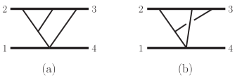
Figure 28: Planar and nonplanar triangle integrals which appear in the cuts in Fig. 12(a).

Similarly, following the steps described above we can construct MB representations which depend on three parameters for the integral in Fig. 28(a) and eight parameters for the integral in Fig. 28(b). Upon specification of contours however they become more complicated, involving several integrals of lower dimension which are needed for the contours to take the standard straight line form. We do not include them explicitly here. Despite these superficial differences, it turns out that the two integrals have identical leading $\ln(-t)$-dependent term:

$$I_{\text{Fig.}\;\ref{VV'}\text{(a)}}\Big{|}_{\ln(-t)\;\text{term}}=I_{\text{Fig.}\;\ref{VV'}\text{(b)}}\Big{|}_{\ln(-t)\;\text{term}}=-\left(\frac{i}{(4\pi)^{2}}\right)^{2}\frac{\ln(-t)}{2m_{2}^{2}t}\int_{\cal C}\frac{dz}{2\pi i}\frac{\Gamma(-1-2z)\Gamma^{2}(-z)\Gamma^{3}(1+z)}{\Gamma(-2z)\Gamma(2+z)}\,,$$ (8.48)

where the contour ${\cal C}$ crosses the real axis at $z_{0}=-0.897$. Closing the contour to the right picks up poles at $z=-1/2$ and at all non-negative integers; the corresponding residues are

$$\text{Res}_{z=-1/2}=-\pi^{2}\,,\hskip 42.67912pt\text{Res}_{z=n\geq 0\cap\mathbb{Z}}=\frac{3+4n}{(1+n)^{2}(1+2n)^{2}}\,,$$ (8.49)

and, once resummed, they give

$$I_{\text{Fig.}\;\ref{VV'}\text{(a)}}\Big{|}_{\ln{\bm{q}}^{2}\text{\ term}}=-\frac{1}{768\pi^{2}}\frac{\ln{\bm{q}}^{2}}{m_{2}^{2}\,{\bm{q}}^{2}}\,.$$ (8.50)

As a further example of application of the MB integration techniques we revisit briefly the integrals ${\rm H}[1,1,0,1,1,1,1,0,0]$ and ${\rm H}[1,1,0,0,1,1,1,0,0]$, defined in Eq. (8.1). We discussed them from the point of view of the differential equation for integrals related to the H graph with two cut matter propagators and restricted to the leading small-$t$ logarithmic term and found that, if the latter is chosen as master integral, the former can be reduced. It is not difficult to derive a 7-dimensional MB representation for ${\rm H}[1,1,0,1,1,1,1,0,0]$ and a 5-dimensional MB representation for ${\rm H}[1,1,0,0,1,1,1,0,0]$. Extracting the leading $\ln(-t)=\ln{\bm{q}}^{2}$ coefficients we find that both integrals are proportional to

$$I=-\frac{\ln(-t)}{(4\pi)^{4}}\int_{\cal C}\frac{dz_{1}dz_{2}}{(2\pi i)^{2}}\left(\frac{-\tau_{12}}{m_{1}m_{2}}\right)^{z_{2}}\frac{\Gamma^{3}(-z_{1})\Gamma(1+z_{1})\Gamma((1+z_{2})/2+z_{1})\Gamma(-z_{2})\Gamma((1+z_{2})/2)}{4m_{1}m_{2}\;\Gamma(1-z_{1})}\,,$$ (8.51)

with the contour ${\cal C}$ crossing the real axis at $z_{1}=-0.078$ and $z_{2}=-0.228$. More specifically

$$I={\rm H}[1,1,0,0,1,1,1,0,0]\Big{|}_{\ln(-t)\text{ term}}=-t{\rm H}[1,1,0,1,1,1,1,0,0]\Big{|}_{\ln(-t)\text{ term}}\,,$$ (8.52)

thus recovering the result of the differential equation approach. We note that the argument here shows that ${\rm H}[1,1,0,1,1,1,1,0,0]$ and ${\rm H}[1,1,0,0,1,1,1,0,0]$ obey this relation even without localization on matter poles.

While, as mentioned above, it is difficult to numerically evaluate the MB integrals for physical momenta, other approaches are up for this task. An example is the sector decomposition strategy, as implemented in the computer codes FIESTA 0807.4129 ; 1511.03614 and SecDec Borowka:2012ii . We used the former to verify the result of the analytic result for the scalar H integral in Appendix D.

In Sec. 8.1.4 we have noticed that all integrals related to Fig. 26 by collapse of propagators enter the classical limit of the amplitude only in the combination symmetrized under the remapping $p_{2}\leftrightarrow p_{3}$. As described in Ref. StermanEikonal , in the classical limit and to leading order in the small-$t$ expansion, the matter propagators organize as

$$\frac{1}{2l_{4}\cdot p_{2}+i\epsilon}+\frac{1}{2l_{4}\cdot p_{3}+i\epsilon}\simeq\frac{1}{2l_{4}\cdot p_{2}+i\epsilon}-\frac{1}{2l_{4}\cdot p_{2}-i\epsilon}=-2\pi i\delta(2l_{4}\cdot p_{2})\,,$$ (8.53)

$$\frac{1}{2l_{1}\cdot p_{1}+i\epsilon}+\frac{1}{2l_{1}\cdot p_{4}+i\epsilon}\simeq\frac{1}{2l_{1}\cdot p_{1}+i\epsilon}-\frac{1}{2l_{1}\cdot p_{1}-i\epsilon}=-2\pi i\delta(2l_{1}\cdot p_{1})\,.$$ (8.54)

The arguments of the two Dirac $\delta$-functions are nothing but the on-shell conditions for the two internal matter lines in the classical limit $|l_{i}^{2}|\sim-t\ll p_{i}^{2}$. Thus, the symmetrized combination of integrals, $I_{i}+\bar{I}_{i}$, localizes on the matter poles and this combination can be compared to the results of the differential equations and nonrelativistic integration that enforce this condition. We have indeed verified that the result of the differential equation approach for the leading $\ln(-t)=\ln{\bm{q}}^{2}$ term of scalar integrals related to Fig. 26 by collapse of propagators (i.e. ${\rm H}[1,1,1,1,1,1,1,0,0]$, ${\rm H}[1,1,0,0,1,1,1,0,0]$, ${\rm H}[1,1,0,1,1,1,1,0,0]$, etc.) is reproduced by high-precision numerical integration. Thus, the results obtained by resumming the nonrelativistic velocity expansion in Sec. 7 and through differential equations in Sec. 8.1 and their contribution to graphs 7 and ${\bar{\bf 7}}$ in Sec. 8.1.4 are complete.

9 Scattering Amplitude

In Sec. 6, we used the double copy and generalized unitarity to construct the integrands denoted as graphs $\bm{1}-\bm{8}$, which are shown in Fig. 14. The integration method described in Sec. 7 ultimately trivializes all one and two loop integrals by reducing them to three-dimensional bubble integrals via nonrelativistic expansion. In Sec. 9.1 below, we present results for each diagram up to 7PN.

Of course the cost of analytic tractability is that the answer is formally computed order by order in the nonrelativistic expansion. However, if we retain terms to sufficiently high order in velocity, then we can resum this expansion, yielding our putative all orders in velocity expression for the PM amplitude. The resummation can be reliably performed because relativity imposes strong constraints on the structure of the series in two important ways. First, the series encountered are due to relativistic invariants whose structure is simple enough to identify order by order in velocity. Second, there is a bound for the highest PN order at which new relativistic structures can appear. Beyond this order velocity corrections are solely from structures that are already present at lower orders. The detailed argument is presented in Sec. 9.2.

We employ two methods for resummation. First is resummation by inspection. As we will see below, the series encountered are geometric, binomial, or arcsinh, where a pattern can be clearly identified. These series are collected in Appendix C. Second is resummation by ansatz. A natural ansatz can be formed from the small basis of functions encountered in the case of scalar two-loop integrals, multiplied by arbitrary polynomials of the external four momenta. The free coefficients are then uniquely fixed by comparing to the first several terms in the PN expansion. Both methods yield the same result, and we discuss various checks below. The final result for scattering amplitudes up to 3PM are given in Eq. (9.3).

9.1 Post-Newtonian Expansion

We can mechanically integrate graphs $\bm{1}-\bm{8}$ using the methods of Sec. 7. This involves expanding the integrands in the nonrelativistic limit, and we do this by assigning the scalings $p_{1}\cdot p_{2}\sim\rho^{2}\,,E_{i}\sim\rho\,,m_{i}\sim\rho$, and then expanding order by order in large $\rho$. This generally leads to much simpler expressions compared to expanding in large $m_{i}$ everywhere since functions of $p_{1}\cdot p_{2}$ and $E_{i}$ are kept intact to all orders in velocity. Our results up to 7PN are

$${\bf 1} =-\frac{2m_{1}^{6}m_{2}^{6}(1-2\sigma^{2})^{3}}{E^{2}}\int\frac{d^{D-1}\bm{\ell}_{1}}{(2\pi)^{D-1}}\frac{d^{D-1}\bm{\ell}_{2}}{(2\pi)^{D-1}}\frac{1}{\bm{\ell}_{1}^{2}(\bm{\ell}_{2}-\bm{\ell}_{1})^{2}(\bm{\ell}_{2}+\bm{q})^{2}(\bm{\ell}_{1}^{2}+2\bm{p}\bm{\ell}_{1})(\bm{\ell}_{2}^{2}+2\bm{p}\bm{\ell}_{2})}\,,$$

$$\overline{\bf 1} =0\,,$$

$${\bf 2} =-{m_{1}^{2}m_{2}^{6}(2\sigma^{2}-1)E\bm{p}^{2}\over 32E_{2}^{3}}\int\frac{d^{D-1}\bm{\ell}}{(2\pi)^{D-1}}\frac{1}{\bm{\ell}^{2}|\bm{\ell}+\bm{q}|(\bm{\ell}^{2}+2\bm{p}\bm{\ell})}\bigg{[}1+\frac{3\bm{p}^{2}}{2E_{2}^{2}}+\frac{15\bm{p}^{4}}{8E_{2}^{4}}+\frac{35\bm{p}^{6}}{16E_{2}^{6}}+\cdots\bigg{]}$$

$$\quad+{m_{1}^{2}m_{2}^{5}(m_{2}+4m_{1}\sigma-5m_{2}\sigma^{2}-8m_{1}\sigma^{3})\over 192\pi^{2}E_{2}^{2}}\bigg{[}1+\frac{\bm{p}^{2}}{E_{2}^{2}}+\frac{\bm{p}^{4}}{E_{2}^{4}}+\frac{\bm{p}^{6}}{E_{2}^{6}}+\frac{\bm{p}^{8}}{E_{2}^{8}}+\frac{\bm{p}^{10}}{E_{2}^{10}}+\cdots\bigg{]}$$

$$\quad-{\sigma^{2}m_{1}^{4}m_{2}^{4}\over 12\pi^{2}E_{1}E_{2}}\bigg{[}1+{\left(E_{1}^{3}+E_{2}^{3}\right)\over 3E_{1}^{2}E_{2}^{2}E}{\bm{p}}^{2}+\frac{\left(E_{1}^{5}+E_{2}^{5}\right)}{5E_{1}^{4}E_{2}^{4}E}{\bm{p}}^{4}+\frac{\left(E_{1}^{7}+E_{2}^{7}\right)}{7E_{1}^{6}E_{2}^{6}E}{\bm{p}}^{6}+\frac{\left(E_{1}^{9}+E_{2}^{9}\right)}{9E_{1}^{8}E_{2}^{8}E}{\bm{p}}^{8}$$

$$\quad+\frac{\left(E_{1}^{11}+E_{2}^{11}\right)}{11E_{1}^{10}E_{2}^{10}E}{\bm{p}}^{10}+\cdots\bigg{]}$$

$$\quad+{m_{1}^{4}m_{2}^{2}E\bm{p}^{2}\over 36\pi^{2}E_{1}^{3}}\bigg{[}1+\frac{6\bm{p}^{2}}{5E_{1}^{2}}+\frac{9\bm{p}^{4}}{7E_{1}^{4}}+\frac{4\bm{p}^{6}}{3E_{1}^{6}}+\frac{15\bm{p}^{8}}{11E_{1}^{8}}+\cdots\bigg{]}$$

$$\quad+{m_{1}^{4}m_{2}^{2}\bm{p}^{2}\over 36\pi^{2}E_{1}^{2}}\bigg{[}1+\frac{3\bm{p}^{2}}{5E_{1}^{2}}+\frac{3\bm{p}^{4}}{7E_{1}^{4}}+\frac{\bm{p}^{6}}{3E_{1}^{6}}+\frac{3\bm{p}^{8}}{11E_{1}^{8}}+\cdots\bigg{]}$$

$$\quad+{m_{1}^{4}m_{2}^{2}\bm{p}^{2}\over 36\pi^{2}E_{1}E_{2}}\bigg{[}1+{\left(E_{1}^{3}+E_{2}^{3}\right)\over 5E_{1}^{2}E_{2}^{2}E}{\bm{p}}^{2}+\frac{3\left(E_{1}^{5}+E_{2}^{5}\right)}{35E_{1}^{4}E_{2}^{4}E}{\bm{p}}^{4}+\frac{\left(E_{1}^{7}+E_{2}^{7}\right)}{21E_{1}^{6}E_{2}^{6}E}{\bm{p}}^{6}+\frac{\left(E_{1}^{9}+E_{2}^{9}\right)}{33E_{1}^{8}E_{2}^{8}E}{\bm{p}}^{8}+\cdots\bigg{]}$$

$$\quad+{m_{1}^{2}m_{2}^{6}(2\sigma^{2}-1)E\over 768\pi^{2}E_{2}^{3}}\bigg{[}1+{7\bm{p}^{2}\over 2E_{2}^{2}}+{51\bm{p}^{4}\over 8E_{2}^{4}}+{151\bm{p}^{6}\over 16E_{2}^{6}}+{1615\bm{p}^{8}\over 128E_{2}^{8}}+{4065\bm{p}^{10}\over 256E_{2}^{10}}+\cdots\bigg{]}\,,$$

$$\overline{\bf 2} =-{\sigma m_{1}^{3}m_{2}^{5}(2\sigma^{2}-1)\over 24\pi^{2}E_{2}^{2}}\bigg{[}1+\frac{\bm{p}^{2}}{E_{2}^{2}}+\frac{\bm{p}^{4}}{E_{2}^{4}}+\frac{\bm{p}^{6}}{E_{2}^{6}}+\frac{\bm{p}^{8}}{E_{2}^{8}}+\frac{\bm{p}^{10}}{E_{2}^{10}}+\cdots\bigg{]}$$

$$\quad-{\sigma^{2}m_{1}^{2}m_{2}^{6}\over 64\pi^{2}E_{2}^{2}}\bigg{[}1-\frac{\bm{p}^{2}}{3E_{2}^{2}}-\frac{5\bm{p}^{4}}{3E_{2}^{4}}-\frac{3\bm{p}^{6}}{E_{2}^{6}}-\frac{13\bm{p}^{8}}{3E_{2}^{8}}-\frac{17\bm{p}^{10}}{3E_{2}^{10}}+\cdots\bigg{]}$$

$$\quad+{\sigma m_{1}^{2}m_{2}^{6}(2\sigma E_{1}E_{2}-m_{1}m_{2})\over 96\pi^{2}E_{2}^{4}}\bigg{[}1+\frac{2\bm{p}^{2}}{E_{2}^{2}}+\frac{3\bm{p}^{4}}{E_{2}^{4}}+\frac{4\bm{p}^{6}}{E_{2}^{6}}+\frac{5\bm{p}^{8}}{E_{2}^{8}}+\frac{6\bm{p}^{10}}{E_{2}^{10}}+\cdots\bigg{]}$$

$$\quad-{\sigma^{2}m_{1}^{4}m_{2}^{4}\over 24\pi^{2}E_{1}E_{2}}\bigg{[}1+{\left(E_{1}^{3}+E_{2}^{3}\right)\over 3E_{1}^{2}E_{2}^{2}E}{\bm{p}}^{2}+\frac{\left(E_{1}^{5}+E_{2}^{5}\right)}{5E_{1}^{4}E_{2}^{4}E}{\bm{p}}^{4}+\frac{\left(E_{1}^{7}+E_{2}^{7}\right)}{7E_{1}^{6}E_{2}^{6}E}{\bm{p}}^{6}+\frac{\left(E_{1}^{9}+E_{2}^{9}\right)}{9E_{1}^{8}E_{2}^{8}E}{\bm{p}}^{8}$$

$$\quad\hskip 85.35826pt+\frac{\left(E_{1}^{11}+E_{2}^{11}\right)}{11E_{1}^{10}E_{2}^{10}E}{\bm{p}}^{10}+\cdots\bigg{]}$$

$$\quad+{m_{1}^{4}m_{2}^{2}\bm{p}^{2}\over 72\pi^{2}E_{1}^{2}}\bigg{[}1+\frac{3\bm{p}^{2}}{5E_{1}^{2}}+\frac{3\bm{p}^{4}}{7E_{1}^{4}}+\frac{\bm{p}^{6}}{3E_{1}^{6}}+\frac{3\bm{p}^{8}}{11E_{1}^{8}}+\cdots\bigg{]}$$

$$\quad+{Em_{1}^{4}m_{2}^{2}\bm{p}^{2}\over 72\pi^{2}E_{1}^{3}}\bigg{[}1+\frac{6\bm{p}^{2}}{5E_{1}^{2}}+\frac{9\bm{p}^{4}}{7E_{1}^{4}}+\frac{4\bm{p}^{6}}{3E_{1}^{6}}+\frac{15\bm{p}^{8}}{11E_{1}^{8}}+\cdots\bigg{]}$$

$$\quad+{m_{1}^{4}m_{2}^{2}\bm{p}^{2}\over 72\pi^{2}E_{1}E_{2}}\bigg{[}1+{\left(E_{1}^{3}+E_{2}^{3}\right)\over 5E_{1}^{2}E_{2}^{2}E}{\bm{p}}^{2}+\frac{3\left(E_{1}^{5}+E_{2}^{5}\right)}{35E_{1}^{4}E_{2}^{4}E}{\bm{p}}^{4}+\frac{\left(E_{1}^{7}+E_{2}^{7}\right)}{21E_{1}^{6}E_{2}^{6}E}{\bm{p}}^{6}+\frac{\left(E_{1}^{9}+E_{2}^{9}\right)}{33E_{1}^{8}E_{2}^{8}E}{\bm{p}}^{8}+\cdots\bigg{]}\,,$$

$${\bf 3} =0\,,$$

$${\bf 4} ={(2\sigma^{2}-1)(4\sigma^{2}-1)m_{1}^{4}m_{2}^{6}\over 8E_{2}E}\int\frac{d^{D-1}\bm{\ell}}{(2\pi)^{D-1}}\frac{1}{\bm{\ell}^{2}|\bm{\ell}+\bm{q}|(\bm{\ell}^{2}+2\bm{p}\bm{\ell})}\bigg{[}1+\frac{\bm{p}^{2}}{2E_{2}^{2}}+\frac{3\bm{p}^{4}}{8E_{2}^{4}}+\frac{5\bm{p}^{6}}{16E_{2}^{6}}+\cdots\bigg{]}$$

$$\quad+{\sigma m_{1}^{3}m_{2}^{5}(4\sigma^{2}-1)\over 48\pi^{2}E_{2}^{2}}\bigg{[}1+\frac{\bm{p}^{2}}{E_{2}^{2}}+\frac{\bm{p}^{4}}{E_{2}^{4}}+\frac{\bm{p}^{6}}{E_{2}^{6}}+\frac{\bm{p}^{8}}{E_{2}^{8}}+\frac{\bm{p}^{10}}{E_{2}^{10}}+\cdots\bigg{]}$$

$$\quad-{m_{1}^{4}m_{2}^{6}(2\sigma^{2}-1)(4\sigma^{2}-1)\over 128\pi^{2}E_{2}^{3}E}\bigg{[}1+{5\bm{p}^{2}\over 4E_{2}^{2}}+{11\bm{p}^{4}\over 8E_{2}^{4}}+{93\bm{p}^{6}\over 64E_{2}^{6}}+{193\bm{p}^{8}\over 128E_{2}^{8}}+{793\bm{p}^{10}\over 512E_{2}^{10}}+\cdots\bigg{]}+\{1\leftrightarrow 2\}\,,$$

$$\overline{\bf 4} ={\sigma m_{1}^{3}m_{2}^{5}(4\sigma^{2}-1)\over 24\pi^{2}E_{2}^{2}}\bigg{[}1+\frac{\bm{p}^{2}}{E_{2}^{2}}+\frac{\bm{p}^{4}}{E_{2}^{4}}+\frac{\bm{p}^{6}}{E_{2}^{6}}+\frac{\bm{p}^{8}}{E_{2}^{8}}+\frac{\bm{p}^{10}}{E_{2}^{10}}+\cdots\bigg{]}+\{1\leftrightarrow 2\}\,,$$

$${\bf 5} =-{\sigma m_{1}^{2}m_{2}^{5}(12\sigma^{2}m_{1}+\sigma m_{2}-6m_{1})\over 96\pi^{2}E_{2}^{2}}\bigg{[}1+\frac{\bm{p}^{2}}{E_{2}^{2}}+\frac{\bm{p}^{4}}{E_{2}^{4}}+\frac{\bm{p}^{6}}{E_{2}^{6}}+\frac{\bm{p}^{8}}{E_{2}^{8}}+\frac{\bm{p}^{10}}{E_{2}^{10}}+\cdots\bigg{]}$$

$$\quad-{\bm{p}^{2}\sigma m_{1}m_{2}^{5}E^{2}\over 48\pi^{2}E_{2}^{4}}\bigg{[}1+\frac{2\bm{p}^{2}}{E_{2}^{2}}+\frac{3\bm{p}^{4}}{E_{2}^{4}}+\frac{4\bm{p}^{6}}{E_{2}^{6}}+\frac{5\bm{p}^{8}}{E_{2}^{8}}+\cdots\bigg{]}\,,$$

$${\bf 6} =-{\sigma^{2}m_{1}^{2}m_{2}^{6}\over 24\pi^{2}E_{2}^{2}}\bigg{[}1+\frac{\bm{p}^{2}}{E_{2}^{2}}+\frac{\bm{p}^{4}}{E_{2}^{4}}+\frac{\bm{p}^{6}}{E_{2}^{6}}+\frac{\bm{p}^{8}}{E_{2}^{8}}+\frac{\bm{p}^{10}}{E_{2}^{10}}+\cdots\bigg{]}\,,$$

$$\bf 7 +\overline{\bf 7}={(2\sigma^{2}-1)^{2}m_{1}^{4}m_{2}^{4}\over 16\pi^{2}E_{1}E_{2}}\bigg{[}1+{\left(E_{1}^{3}+E_{2}^{3}\right)\over 3E_{1}^{2}E_{2}^{2}E}{\bm{p}}^{2}+\frac{\left(E_{1}^{5}+E_{2}^{5}\right)}{5E_{1}^{4}E_{2}^{4}E}{\bm{p}}^{4}+\frac{\left(E_{1}^{7}+E_{2}^{7}\right)}{7E_{1}^{6}E_{2}^{6}E}{\bm{p}}^{6}+\frac{\left(E_{1}^{9}+E_{2}^{9}\right)}{9E_{1}^{8}E_{2}^{8}E}{\bm{p}}^{8}$$

$$\quad+\frac{\left(E_{1}^{11}+E_{2}^{11}\right)}{11E_{1}^{10}E_{2}^{10}E}{\bm{p}}^{10}+\cdots\bigg{]}\,,$$

$${\bf 8} =0\,.$$ (9.1)

Here for every equation we have omitted a factor of $\frac{1}{2}(8\pi G)^{3}\ln\bm{q}^{2}$ for the finite terms and a factor of $(8\pi G)^{3}$ for the remaining infrared divergent integrals. We have not included a factor of $1/(4E_{1}E_{2})$ for nonrelativistic normalization. Moreover, for diagrams $\bf 4$ and $\overline{\bf 4}$, we denote by $\{1\leftrightarrow 2\}$ contributions obtained from swapping the mass and energy subscripts in all terms. The results above are for the individual diagrams $\bm{1}-\bm{8}$, and do not include contributions from topologies related by flipping the diagram. Graphs $\overline{\bf 1},\overline{\bf 2},\overline{\bf 4},\overline{\bf 7}$ are related to graphs $\bf{1},\bf{2},\bf{4},\bf{7}$ by crossing, i.e. by swapping the external momenta $p_{2}\leftrightarrow p_{3}$ or equivalently $p_{1}\leftrightarrow p_{4}$. We refer the reader to Table 1.

Note that judicious further expansion of factors of $E_{i}$ in some places can lead to even simpler results. In particular, series resummation often yields factors of $E_{i}$ and $m_{i}$ that cancel in the final result (see Appendix C). For example, in graph $\bf 6$, expanding the factor of $m_{2}^{2}/E_{2}^{2}$ in large $m_{2}$ cancels the geometric series in $\bm{p}^{2}/E_{2}^{2}$, yielding a result that is exact at 2PN. This is expected since it follows from the topology of $\bf 6$ that its nonrelativistic expansion is in $|\bm{q}|/m_{i}$, and there are no velocity corrections from integration.

We see that graphs $\bf 1\,,\overline{\bf 1}\,,\bf 3$, and $\bf 8$ are zero except for a contribution from iterations of lower order processes which will cancel in the matching with the EFT.

9.2 Post-Minkowskian Expansion

The results for graphs $\bm{1}-\bm{8}$ above are expressed in terms of series that have a substantially simple structure order by order in $\bm{p}^{2}$. This simplicity is of course due to relativistic invariance. However, even if it is trivial by inspection to resum all orders in velocity, it is natural to be suspicious since any finite number of terms in a generic series has no bearing on the full function. Nevertheless, apart from the verification of certain graphs by fully relativistic methods, we believe that our resummation is trustworthy due to the following argument.

The underlying worry about resummation is that extrapolation may fail due to the appearance of new velocity-dependent structures at some high order. Note, however, that the velocity expansion is not an arbitrary series. Rather, it is strongly constrained by relativistic invariance of the underlying theory and any new velocity-dependent structure must originate from a new fully relativistic one.

There is a simple argument from dimensional analysis that forbids new relativistic structures from appearing at arbitrarily high order in the PN expansion. First, recall that the two loop scattering amplitude has mass dimension six. Since every graph has seven propagators and the integration measure has mass dimension eight, the numerator of the integrand must have mass dimension twelve. If we assume conservatively that the entire mass dimension of the numerator is due to $\bm{p}$, then the numerator scales at most as $\bm{v}^{12}$ which, together with the $G^{3}$ factor, is of 8PN order. This logic suggests that beyond 8PN no new velocity dependent structure will appear and all velocity corrections are from the expansion of structures that are already present at lower orders.

The 8PN bound argued above only uses dimensional analysis and can be refined by noting that the mass dimension of the numerator cannot be due entirely to $\bm{p}$. In particular, the numerator must provide some dimensionful factors of $\bm{q}$ in order to produce a classical contribution. We thus need to consider the numerator dependence on factors of $p\cdot\ell$ and $\ell^{2}$, where $p$ is an external four momentum and $\ell$ is a loop four momentum. Other numerator factors which are independent of the loop variables and depend only on $p_{1}\cdot p_{2}$ and $\bm{q}^{2}$, are effectively constant and do not affect the integration. Consequently, these spectator factors can be separated from the actual integration and do not produce new factors of $\bm{p}$ upon integration. Given the $\bm{q}$ and $\bm{v}$ scaling of graviton momenta in the potential region discussed in Sec. 2, a generic combination $(p\cdot\ell)^{a}(\ell^{2})^{b}$ scales at most as $|{\bm{q}}|^{a+2b}|{\bm{v}}|^{a+2b}$. In deriving this we focused on the highest power of the velocity as this automatically covers any weaker dependence on $|{\bm{v}}|$. The upshot is that, for the non-spectator terms in the numerator, the scaling of the numerator in $v$ is equal to the scaling of the numerator in $|{\bm{q}}|$, thus lowering the bound by a factor of two.

Concretely, consider a diagram with $n_{G}$ graviton propagators and $n_{M}$ matter propagators. Graphs ${\bf 1}-{\bf 8}$ all have exactly $n_{G}+n_{M}=7$ propagators. Using this, together with the fact that the measure scales as $|{\bm{q}}|^{8}$ and the propagator denominators scale as $|{\bm{q}}|^{2n_{G}+n_{M}}$, we learn that the numerator must scale at most as $|{\bm{q}}|^{n_{G}-1}$. Any higher $\bm{q}$ scaling will produce a quantum correction. Hence the numerator scales at most as $|{\bm{v}}|^{n_{G}-1}$. Since the maximum number for $n_{G}$ in our set of diagrams is five, we obtain a global bound at 4PN as the highest order at which new $\bm{p}$-dependent structures can arise.

Still the above argument can be refined further if we consider information about individual diagrams. For example, we know from the possible relativistic invariants of diagrams $\bf 3$ and $\bf 6$ that they are expansions in $\bm{q}/m$ and not $\bm{p}/m\sim\bm{v}$. These diagrams are therefore exact at 2PN, and in fact the series in the result for $\bf 6$ in Eq. (9.1) cancels with the factor of $m_{2}^{2}/E_{2}^{2}$. Another example is given by diagrams such as $\bf 1$, $\bf 2$, and $\bf 4$, which have $n_{M}>2$ matter propagators. For these diagrams the numerator terms that contribute to the static or 2PN order scale as $|\bm{p}|^{n_{M}-2}$ in order to cancel the extra factor of $|\bm{p}|^{2-n_{M}}$ from the matter propagators. This lowers the bound to 2PN for diagrams with four matter propagators and to 3PN for diagrams with three matter propagators. As a final example, we know from the mechanics of two loop integration that diagram $\bf 8$ will not develop the required $\ln\bm{q}^{2}$ structure that makes a contribution at two loop order classical, and therefore it vanishes to all orders.

The above arguments imply that all relativistic invariants are already manifest in the 7PN results in Eq. (9.1), and hence that resummation can be reliably performed. For most of the series encountered, there is immediately an obvious pattern that can be extended naturally to all orders, while others require some sleuthing. Details are given in Appendix C. Upon resummation, we obtain the following all orders in velocity expressions:

$${\bf 1} =-\frac{2m_{1}^{6}m_{2}^{6}(1-2\sigma^{2})^{3}}{E^{2}}\int\frac{d^{D-1}\bm{\ell}_{1}}{(2\pi)^{D-1}}\frac{d^{D-1}\bm{\ell}_{2}}{(2\pi)^{D-1}}\frac{1}{\bm{\ell}_{1}^{2}(\bm{\ell}_{2}-\bm{\ell}_{1})^{2}(\bm{\ell}_{2}+\bm{q})^{2}(\bm{\ell}_{1}^{2}+2\bm{p}\bm{\ell}_{1})(\bm{\ell}_{2}^{2}+2\bm{p}\bm{\ell}_{2})}\,,$$

$$\overline{\bf 1} =0\,,$$

$${\bf 2} =-{m_{1}^{2}m_{2}^{3}(2\sigma^{2}-1)E\bm{p}^{2}\over 32}\int\frac{d^{D-1}\bm{\ell}}{(2\pi)^{D-1}}\frac{1}{\bm{\ell}^{2}|\bm{\ell}+\bm{q}|(\bm{\ell}^{2}+2\bm{p}\bm{\ell})}-{m_{1}^{2}m_{2}^{3}\sigma(6m_{1}\sigma^{2}+3\sigma m_{2}-11m_{1})\over 192\pi^{2}}$$

$$\quad-{m_{1}^{4}m_{2}^{5}(\sigma^{2}-1)(2\sigma^{2}-1)\over 256\pi^{2}E\bm{p}^{2}}-{m_{1}^{3}m_{2}^{3}(2\sigma^{2}+1)\over 12\pi^{2}}{{\rm arcsinh}\sqrt{\sigma-1\over 2}\over\sqrt{\sigma^{2}-1}}\,,$$

$$\overline{\bf 2} =-{m_{1}^{2}m_{2}^{3}\sigma(12\sigma^{2}m_{1}+3\sigma m_{2}-10m_{1})\over 192\pi^{2}}-{m_{1}^{3}m_{2}^{3}(2\sigma^{2}+1)\over 24\pi^{2}}{{\rm arcsinh}\sqrt{\sigma-1\over 2}\over\sqrt{\sigma^{2}-1}}\,,$$

$${\bf 3} =0\,,$$

$${\bf 4} ={(2\sigma^{2}-1)(4\sigma^{2}-1)m_{1}^{4}m_{2}^{4}m\over 8E}\int\frac{d^{D-1}\bm{\ell}}{(2\pi)^{D-1}}\frac{1}{\bm{\ell}^{2}|\bm{\ell}+\bm{q}|(\bm{\ell}^{2}+2\bm{p}\bm{\ell})}+{\sigma m_{1}^{3}m_{2}^{3}(4\sigma^{2}-1)\over 24\pi^{2}}$$

$$\quad-{m_{1}^{4}m_{2}^{4}(2\sigma^{2}-1)(4\sigma^{2}-1)(E-m)\over 64\pi^{2}E\bm{p}^{2}}\,,$$

$$\overline{\bf 4} ={\sigma m_{1}^{3}m_{2}^{3}(4\sigma^{2}-1)\over 12\pi^{2}}\,,$$

$${\bf 5} =-\frac{2\sigma m_{1}^{2}m_{2}^{3}\left(14\sigma^{2}m_{1}+\sigma m_{2}-8m_{1}\right)}{192\pi^{2}}\,,$$

$${\bf 6} =-{\sigma^{2}m_{1}^{2}m_{2}^{4}\over 24\pi^{2}}\,,$$

$${\bf 7} +\overline{\bf 7}={m_{1}^{3}m_{2}^{3}(2\sigma^{2}-1)^{2}\over 8\pi^{2}}{{\rm arcsinh}\sqrt{\sigma-1\over 2}\over\sqrt{\sigma^{2}-1}}\,,$$

$${\bf 8} =0\,,$$ (9.2)

again omitting the same prefactors as in Eq. (9.1). Note that for diagrams $\bf 4$ and $\overline{\bf 4}$ the contributions denoted by $\{1\leftrightarrow 2\}$ in Eq. (9.1) are included in Eq. (9.2). For some diagrams such as ${\bf 7}+\overline{\bf 7}$, we have checked the result using relativistic integration (see Sec. 8).

The total amplitude is then obtained by summing these contributions and including the relabeling given in Table 1. We present here our final expression for the 3PM scattering amplitude, ${\cal M}_{3}$, along with expressions for the 1PM and 2PM amplitudes, ${\cal M}_{1}$ and ${\cal M}_{2}$, for completeness:

$${\cal M}_{1} =-{4\pi G\nu^{2}m^{2}\over\gamma^{2}\xi\bm{q}^{2}}(1-2\sigma^{2})\,,$$ (9.3)

$${\cal M}_{2} =-{3\pi^{2}G^{2}\nu^{2}m^{3}\over 2\gamma^{2}\xi|\bm{q}|}(1-5\sigma^{2})+{32\pi^{2}G^{2}\nu^{4}m^{5}(1-2\sigma^{2})^{2}\over\gamma^{3}\xi}\int\frac{d^{D-1}\bm{\ell}_{1}}{(2\pi)^{D-1}}\frac{1}{\bm{\ell}^{2}(\bm{\ell}+\bm{q})^{2}(\bm{\ell}^{2}+2\bm{p}\bm{\ell})}\,,$$

$${\cal M}_{3} =\frac{\pi G^{3}\nu^{2}m^{4}\ln\bm{q}^{2}}{6\gamma^{2}\xi}\bigg{[}3-6\nu+206\nu\sigma-54\sigma^{2}+108\nu\sigma^{2}+4\nu\sigma^{3}$$

$$\quad-{48\nu\left(3+12\sigma^{2}-4\sigma^{4}\right){\rm arcsinh}\sqrt{\sigma-1\over 2}\over\sqrt{\sigma^{2}-1}}-{18\nu\gamma\left(1-2\sigma^{2}\right)\left(1-5\sigma^{2}\right)\over\left(1+\gamma\right)\left(1+\sigma\right)}\bigg{]}$$

$$\quad+{8\pi^{3}G^{3}\nu^{4}m^{6}\over\gamma^{4}\xi}\bigg{[}{3\gamma\left(1-2\sigma^{2}\right)\left(1-5\sigma^{2}\right)}\int\frac{d^{D-1}\bm{\ell}}{(2\pi)^{D-1}}\frac{1}{\bm{\ell}^{2}|\bm{\ell}+\bm{q}|(\bm{\ell}^{2}+2\bm{p}\bm{\ell})}$$

$$\quad-{32m^{2}\nu^{2}\left(1-2\sigma^{2}\right)^{3}}\int\frac{d^{D-1}\bm{\ell}_{1}}{(2\pi)^{D-1}}\frac{d^{D-1}\bm{\ell}_{2}}{(2\pi)^{D-1}}\frac{1}{\bm{\ell}_{1}^{2}(\bm{\ell}_{2}-\bm{\ell}_{1})^{2}(\bm{\ell}_{2}+\bm{q})^{2}(\bm{\ell}_{1}^{2}+2\bm{p}\bm{\ell}_{1})(\bm{\ell}_{2}^{2}+2\bm{p}\bm{\ell}_{2})}\bigg{]}\,.$$

We remind the reader that here we use center-of-mass coordinates where the incoming and outgoing particle momenta are $\pm\bm{p}$ and $\pm(\bm{p}-\bm{q})$, respectively. We have included the overall normalization factor $(8\pi G)^{3}$ as well as the nonrelativistic normalization factor $1/4E_{1}E_{2}$, where $E_{1,2}=\sqrt{\bm{p}^{2}+m_{1,2}^{2}}$. We define the total mass $m=m_{1}+m_{2}$, the symmetric mass ratio $\nu=m_{1}m_{2}/m^{2}$, the total energy $E=E_{1}+E_{2}$, the symmetric energy ratio $\xi=E_{1}E_{2}/E^{2}$, the energy-mass ratio $\gamma=E/m$, and the relativistic kinematic invariant $\sigma={p_{1}\cdot p_{2}\over m_{1}m_{2}}$.

The remaining integrals in Eq. (9.3) are IR divergent and manifest the iterative structure through factors of the tree-level and one loop triangle scalar coefficients, given respectively by $(1-2\sigma^{2})$ and $(1-5\sigma^{2})$. The integrals in ${\cal M}_{2}$ and ${\cal M}_{3}$ that are proportional to $(1-2\sigma^{2})^{2}$ and $(1-2\sigma^{2})^{3}$ represent the double and triple iterations of tree-level exchange. The integral in ${\cal M}_{3}$ that is proportional to $(1-2\sigma^{2})(1-5\sigma^{2})$ represents the iteration of the tree-level exchange and the one loop triangle. Note that the $(1-5\sigma^{2})$ factor arises from combining the IR divergent integrals in graphs $\bf 2$ and $\bf 4$. We have also computed these IR pieces by using factorization properties of the full amplitude in transverse impact parameter space. As we will see in the next section, these IR artifacts will cancel with similar contributions from the EFT. This is of course guaranteed because the two theories describe the same infrared dynamics, but nonetheless provides a nontrivial check.

As an alternative to resummation by inspection, we can build an ansatz from the small number of simple functional basis elements encountered in the case of scalar two loop integrals discussed in Sec. 7. The basis functions correspond to the primitive topologies given by the scalar double triangle diagram, the scalar box triangle diagram, and the scalar double triangle prime diagram, which are respectively given by

$${\cal O}_{1}=1\,,\quad{\cal O}_{2}=\frac{E-m}{E\bm{p}^{2}}\,,\quad{\cal O}_{3}={1\over E|\bm{p}|}\left({\rm arcsinh}{|\bm{p}|\over m_{1}}+{\rm arcsinh}{|\bm{p}|\over m_{2}}\right)\,.$$ (9.4)

The ansatz is then

$${\cal M}_{3}^{\rm ansatz}=\tau_{1}{\cal O}_{1}+\tau_{2}{\cal O}_{2}+\tau_{3}{\cal O}_{3}\,,$$ (9.5)

where the $\tau_{i}$ are arbitrary polynomial functions of $m_{1}^{2}$, $m_{2}^{2}$, and $\sigma$ with correct overall mass dimension. Performing the fit to explicit results, we find that these functions are already uniquely fixed by the 6PN results. Consequently, the 7PN terms of the explicit calculation provide a nontrivial verification of the resummed amplitude in Eq. (9.3). The uniqueness and the simplicity of the all-orders result in Eq. (9.3) are remarkable.

A feature of the 3PM amplitude in Eq. (9.3) is that it contains a mass singularity due to the arcsinh factor. This factor, which is proportional to the sum of particle rapidities, ${\rm arctanh}\,|{{\bm{p}}}|/E_{1,2}$, diverges as the two masses become simultaneously small. Taking $m_{1}\sim m_{2}\rightarrow 0$ in the 3PM amplitude we find a logarithmic singularity,

$${\cal M}_{3}\rightarrow-128\pi{G^{3}}{\bm{p}}^{4}\ln{\bm{q}}^{2}\,\ln\Bigl{(}\frac{m_{1}m_{2}}{4{\bm{p}}^{2}}\Bigr{)}+\cdots=-8\pi{G^{3}}s^{2}\ln(-t)\,\ln\Bigl{(}\frac{m_{1}m_{2}}{s}\Bigr{)}+\cdots\,,$$ (9.6)

where we display only the singular term in the IR finite part. At first sight this might seem surprising because scattering amplitudes in quantum gravity do not have such singularities Weinberg:1965nx ; 1101.1524 ; Akhoury:2011kq . However, as we explain in Sec. 12.1, this singularity arises in the classical potential region, and an interchange of limits of small mass with small momentum transfer prevents the cancellation of mass singularities that would occur in the quantum theory.

10 Effective Field Theory

The culmination of the previous sections is the 3PM scattering amplitude shown in Eq. (9.3). Employing the EFT framework described in Ref. CliffIraMikhailClassical we can now translate the 1PM, 2PM and 3PM amplitudes into the classical Hamiltonian describing the conservative dynamics of a compact binary system. Our approach is a straightforward EFT matching calculation. First, we compute the two particle scattering amplitudes in the EFT mediated by a generic classical Hamiltonian compatible with the potential in Eq. (1.2). Next, the free coefficients of the Hamiltonian are fixed by matching the EFT amplitudes to the amplitudes of the full theory. In the present section we briefly recall the details of the EFT and the matching procedure.

As we will see, the EFT framework described here offers a useful tool for checking that a given potential is consistent, or that two potentials in different gauges are physically equivalent, by computing on-shell amplitudes, which are gauge invariant and independent of field variables. In particular, in Sec. 11.2, we take known potentials, such as the 4PN potential from literature and the Schwarzschild potential, and verify that the resulting amplitudes agree with Eq. (9.3) in the overlap regions. An alternative approach, based on the EOB framework, was described in Ref. DamourTwoLoop .

10.1 Formalism

The effective theory describes two nonrelativistic scalar fields $\phi_{1}$ and $\phi_{2}$, with masses $m_{1}$ and $m_{2}$, interacting through a long distance potential. The Lagrangian for this system is

$${\cal L}= \int{d^{D-1}\bm{k}\over(2\pi)^{D-1}}\,\phi_{1}^{\dagger}(-\bm{k})\left(i\partial_{t}-\sqrt{\bm{k}^{2}+m_{1}^{2}}\right)\phi_{1}(\bm{k})+\int{d^{D-1}\bm{k}\over(2\pi)^{D-1}}\,\phi_{2}^{\dagger}(-\bm{k})\left(i\partial_{t}-\sqrt{\bm{k}^{2}+m_{2}^{2}}\right)\phi_{2}(\bm{k})$$ (10.1)

$$-\int{d^{D-1}\bm{k}\over(2\pi)^{D-1}}{d^{D-1}\bm{k}^{\prime}\over(2\pi)^{D-1}}\,V(\bm{k},\bm{k}^{\prime})\,\phi_{1}^{\dagger}(\bm{k}^{\prime})\phi_{1}(\bm{k})\phi_{2}^{\dagger}(-\bm{k}^{\prime})\phi_{2}(-\bm{k})\,,$$

where we work in the center of mass frame. The potential is written as a contact operator since it is generated by integrating out potential modes which are off shell. The function $V(\bm{k},\bm{k}^{\prime})$ is parameterized by an ansatz of real rotational invariants composed of $\bm{k}$ and $\bm{k}^{\prime}$. We choose a field basis where $V(\bm{k},\bm{k}^{\prime})$ depends only on the combination $\bm{k}^{2}+\bm{k}^{\prime 2}$ and the momentum transfer $|\bm{k}-\bm{k}^{\prime}|$. Other choices involve combinations that vanish on shell, such as $\bm{k}^{2}-\bm{k}^{\prime 2}$ and $k_{0}-k_{0}^{\prime}$, and are related to our choice by field redefinition. The explicit form of our ansatz is

$$V(\bm{k},\bm{k}^{\prime}) =\sum_{n=1}^{\infty}{(G/2)^{n}(4\pi)^{(D-1)/2}\over|\bm{k}-\bm{k}^{\prime}|^{D-1-n}}\frac{\Gamma\left[(D-1-n)/2\right]}{\Gamma\left[n/2\right]}\,c_{n}\left({\bm{k}^{2}+\bm{k}^{\prime 2}\over 2}\right)$$ (10.2)

$$=\frac{4\pi G}{|\bm{k}-\bm{k}^{\prime}|^{2}}\,c_{1}\left({\bm{k}^{2}+\bm{k}^{\prime 2}\over 2}\right)+\frac{2\pi^{2}G^{2}}{|\bm{k}-\bm{k}^{\prime}|}\,c_{2}\left({\bm{k}^{2}+\bm{k}^{\prime 2}\over 2}\right)-2\pi G^{3}\ln(\bm{k}-\bm{k}^{\prime})^{2}\,c_{3}\left({\bm{k}^{2}+\bm{k}^{\prime 2}\over 2}\right)+\cdots\,,$$

where we work in $D=4-2\epsilon$ dimensions, the coefficient functions $c_{n}$ contain all orders in the velocity expansion, and $n$ labels the order in the PM expansion at which a coefficient becomes relevant. In the second line, the ellipsis contains terms of higher order in the PM expansion, and we have dropped terms that are independent of the momentum transfer since these are contact interactions that do not affect long distance scattering. Note that the normalization adopted here is different from the one in Ref. CliffIraMikhailClassical .

For off-shell kinematics, the potential $V(\bm{k},\bm{k}^{\prime})$ includes quantum corrections that are proportional to off-shell matter propagators through the combination $\bm{k}^{2}+\bm{k}^{\prime 2}$. For on-shell kinematics, the potential can be taken to be purely classical. We have checked that including quantum mechanical corrections to the on-shell potential is not necessary for determining the classical dynamics. Such quantum corrections would lead to classical terms in the amplitude that are, however, infrared divergent and would simply cancel in the matching. For the application of this EFT for determining the full quantum potential and for a discussion of matching with off-shell external kinematics see Ref. Manohar:2000hj .

We can Fourier transform the momentum transfer $|\bm{k}-\bm{k}^{\prime}|$ to its conjugate variable $\bm{r}$, the distance between the two particles in position space. This gives the classical conservative potential between two point particles in Eq. (1.2), where we have set $\bm{k}^{2}=\bm{k}^{\prime 2}=\bm{p}^{2}$ in $c_{n}({\bm{k}^{2}+\bm{k}^{\prime 2}\over 2})$ for on-shell kinematics. Note that our choice of field basis in momentum space corresponds to the so-called isotropic gauge in position space in which the invariant $\bm{p}\cdot\bm{r}$ does not appear.

We identify the interaction potential of the scalar field theory to be the conservative potential for the binary system. Let us elaborate on the reason for this equivalence. The interaction vertex $V$ is defined in the Lagrangian ${\cal L}$ for a second quantized field theory describing two massive scalars. We can mechanically Legendre transform to the Hamiltonian ${\cal H}=\Pi_{1}\frac{\delta{\cal L}}{\delta\phi_{1}}+\Pi_{2}\frac{\delta{\cal L}}{\delta\phi_{2}}-{\cal L}$ of the second quantized field theory, where $\Pi_{i}=\frac{\delta{\cal L}}{\delta\dot{\phi}_{i}}$. Since $V$ has no dependence on $\dot{\phi}_{i}$, it does not affect the conjugate momentum in the second quantized theory. Consequently, the interaction terms from $V$ simply flip sign when going to the Hamiltonian formalism. We then truncate the second quantized Hamiltonian down to the two-particle subspace spanned by the massive scalars, as required by the nonrelativistic limit. The resulting quantity is equal to the first quantized Hamiltonian for the two-particle system, whose corresponding interaction is by definition the conservative potential between classical point particles.

10.2 Scattering Amplitude

The EFT amplitude is given by the sum of iterated bubbles shown in Fig. 29. Note that particle number is conserved in such diagrams; topologies involving pair production of the massive states is kinematically forbidden in the classical nonrelativistic limit. Since the interaction $V(\bm{k},\bm{k}^{\prime})$ is not homogeneous in the coupling constant $G$, the $n$PM amplitude, which scales as ${\cal O}(G^{n})$, receives contributions from all diagrams with at most $n-1$ bubbles.

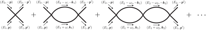
Figure 29: The EFT scattering amplitude is given by a sum of bubble diagrams.

The Feynman rules for the EFT follow from Eq. (10.2) in the usual way. For the propagator of the scalars, it is convenient to define a “two-body” propagator given by the product of the two nonrelativistic propagators comprising a bubble, integrated over the energy component of the loop momentum:

$$i\Delta({\bm{k}}) =\int\frac{d\omega}{2\pi}\frac{i}{\omega-\sqrt{{\bm{k}}^{2}+m_{1}^{2}}}\frac{i}{E-\omega-\sqrt{{\bm{k}}^{2}+m_{2}^{2}}}=\frac{i}{E-\sqrt{{\bm{k}}^{2}+m_{1}^{2}}-\sqrt{{\bm{k}}^{2}+m_{2}^{2}}}\,,$$ (10.3)

where the second equality is obtained by closing the $\omega$ contour either upwards or downwards in the complex plane. We are able to perform this integration over the energy component of the loop momentum since the interaction vertex in Eq. (10.2) has no energy dependence. This leaves us with integration over the spatial component of the loop momenta.

Using the Feynman rules described above, we compute the $n$PM amplitude in the effective theory,

$${\cal M}^{\rm EFT}_{n}=-V(\bm{p},\bm{p}^{\prime})-\sum_{n_{L}=1}^{n-1}\left[\prod_{i=1}^{n_{L}}\int{d^{D-1}\bm{k}_{i}\over(2\pi)^{D-1}}\right]V(\bm{p},\bm{k}_{1})\Delta(\bm{k}_{1})\cdots\Delta(\bm{k}_{n_{L}})V(\bm{k}_{n_{L}},\bm{p}^{\prime})\,,$$ (10.4)

where the second term involving the sum contributes for $n>1$. The loop momenta ${\bm{k}}_{i}$ for $i=1$ to $n_{L}$ are the momenta flowing through the internal matter lines as shown in Fig. 29. We can simplify this integral by expanding the integrand in the classical limit, taking the momentum transfer at each interaction point to scale as $|\bm{k}_{i}-\bm{k}_{i+1}|\sim\bm{q}$, while the degree to which each two-body propagator is off-shell scales as $\bm{k}_{i}^{2}-\bm{p}^{2}\sim\bm{q}$. Expanding the amplitude through the classical order we find

$${\cal M}^{\rm EFT}_{n}=-V(\bm{p},\bm{p}^{\prime})-\sum_{n_{L}=1}^{n-1}\left[\prod_{i=1}^{n_{L}}\int{d^{D-1}\bm{k}_{i}\over(2\pi)^{D-1}}\right]\left[\prod_{i=0}^{n_{L}}{1\over|\bm{k}_{i}-\bm{k}_{i+1}|^{2}}\right]\left[\prod_{i=1}^{n_{L}}{1\over\bm{k}_{i}^{2}-\bm{p}^{2}}\right]{\cal N}^{\rm EFT}_{n_{L}}\,,$$ (10.5)

where we have introduced $\bm{k}_{0}=\bm{p}$ and $\bm{k}_{n_{L}+1}=\bm{p}^{\prime}$. The first term is the tree level contribution given by the potential evaluated on shell, and the second term captures the classical contributions from the sum of iterated bubbles. The poles $\bm{k}_{i}^{2}-\bm{p}^{2}$ come from the expansion of the two-body propagators $\Delta$ in Eq. (10.4), while the poles $|\bm{k}_{i}-\bm{k}_{i+1}|^{2}$ come from the expansion of the vertices $V$ in Eq. (10.4). The numerator ${\cal N}^{\rm EFT}_{n_{L}}$ is a regular function whose momentum dependence may cancel factors in the denominator.

We can map the integral in Eq. (10.5) to the general type treated in Sec. 7 by changing integration variables $\bm{k}_{i}\to\bm{p}+\bm{\ell}_{i}$ for $i=1$ to $n_{L}$. For any one of the loop momenta, the resulting form is that of Eq. (7.8) with $\gamma\leq 1$ and $\alpha,\beta\leq 2$. The poles in $|\bm{k}_{i}-\bm{k}_{i+1}|^{2}$ and $\bm{k}_{i}^{2}-\bm{p}^{2}$ here map to the graviton and matter propagator poles in Eq. (7.8), respectively. As described in Sec. 7, all triangle subdiagrams are evaluated sequentially, while box subdiagrams lead to superclassical iterations, which are infrared divergent and cancel in the matching between full theory and effective theory.

Putting together all of this machinery, we obtain the EFT scattering amplitudes up to 3PM order:

$${\cal M}^{\rm EFT}_{1} =-\frac{4\pi Gc_{1}}{\bm{q}^{2}}\,,$$

$${\cal M}^{\rm EFT}_{2} =-\frac{2\pi^{2}G^{2}c_{2}}{|\bm{q}|}+{\pi^{2}G^{2}\over E\xi|\bm{q}|}\bigg{[}(1-3\xi)c_{1}^{2}+4\xi^{2}E^{2}c_{1}c_{1}^{\prime}\bigg{]}+\int{d^{D-1}{\bm{\ell}}\over(2\pi)^{D-1}}{32E\xi\pi^{2}G^{2}c_{1}^{2}\over\bm{\ell}^{2}(\bm{\ell}+\bm{q})^{2}(\bm{\ell}^{2}+2\bm{p}\bm{\ell})}\,,$$

$${\cal M}^{\rm EFT}_{3} =2\pi G^{3}\ln\bm{q}^{2}c_{3}-{\pi G^{3}\ln\bm{q}^{2}\over E^{2}\xi}\bigg{[}(1-4\xi)c_{1}^{3}-8\xi^{3}E^{4}c_{1}c_{1}^{\prime}{}^{2}-4\xi^{3}E^{4}c_{1}^{2}c_{1}^{\prime\prime}+4\xi^{2}E^{3}c_{2}c_{1}^{\prime}$$

$$\quad\hskip 85.35826pt+4\xi^{2}E^{3}c_{1}c_{2}^{\prime}-2(3-9\xi)\xi E^{2}c_{1}^{2}c_{1}^{\prime}+2E(1-3\xi)c_{1}c_{2}\bigg{]}$$

$$\quad+\int{d^{D-1}{\bm{\ell}}\over(2\pi)^{D-1}}{16\pi^{3}G^{3}c_{1}\left[2E\xi c_{2}-(1-3\xi)c_{1}^{2}-4\xi^{2}E^{2}c_{1}c_{1}^{\prime}\right]\over\bm{\ell}^{2}|\bm{\ell}+\bm{q}|(\bm{\ell}^{2}+2\bm{p}\bm{\ell})}$$

$$\quad-\int{d^{D-1}{\bm{\ell}_{1}}\over(2\pi)^{D-1}}{d^{D-1}{\bm{\ell}_{2}}\over(2\pi)^{D-1}}{256E^{2}\xi^{2}\pi^{3}G^{3}c_{1}^{3}\over\bm{\ell}_{1}^{2}(\bm{\ell}_{1}+\bm{\ell}_{2})^{2}(\bm{\ell}_{2}+\bm{q})^{2}(\bm{\ell}_{1}^{2}+2\bm{p}\bm{\ell}_{1})(\bm{\ell}_{2}^{2}+2\bm{p}\bm{\ell}_{2})}\,,$$ (10.6)

where the dependence of the functions $c_{n}$ on $\bm{p}^{2}$ is kept implicit, while $c_{n}^{\prime}$ and $c_{n}^{\prime\prime}$ denote first and second derivatives with respect to $\bm{p}^{2}$. The unevaluated integrals are IR divergent and manifest the iterative structure through factors of the coefficients $c_{n}$. The integrals in ${\cal M}_{2}^{\rm EFT}$ and ${\cal M}_{3}^{\rm EFT}$ that are proportional to $c_{1}^{2}$ and $c_{1}^{3}$ represent the double and triple iteration of the 1PM potential. The integral in ${\cal M}_{3}^{\rm EFT}$ that depends on the product $c_{1}c_{2}$ represents the iteration of the 1PM potential and 2PM potential.

It is straightforward to extend these results to higher orders in the PM expansion. Note however that our construction here includes only the conservative sector of the effective theory as sufficient for extracting the classical conservative potential at 3PM order. For describing dissipative dynamics and the conservative dynamics beyond 3PM, operators encoding gravitational wave emission must be included in the effective theory. See Sec. 12.3 for further discussion.

10.3 Conservative Potential from Matching

By construction, the effective theory given by Eq. (10.1) captures the same physics described by the full theory for two-to-two scattering of scalars interacting through exchanges of gravitons in the classical potential region. Thus, the full theory and EFT amplitudes must match order by order in the PM expansion,

$${\cal M}_{n}={\cal M}^{\rm EFT}_{n}\,,$$ (10.7)

and this allows us to successively determine the unknown coefficient functions $c_{1}\,,c_{2}\,,c_{3}\,,$… that parameterize the classical potential. In particular, matching at $n$PM order determines the coefficient $c_{n}$ which comes from the tree-level diagram in the EFT and appears linearly in the first term of the amplitudes in Eq. (10.6). The matching at $n$PM involves the lower order coefficients, $c_{i}$ for $i=1$ to $n-1$, through subtraction terms which include infrared divergent integrals. Performing this matching procedure, we obtain the classical conservative Hamiltonian at 3PM order

$$H^{\rm 3PM}(\bm{p},\bm{r}) =\sqrt{\bm{p}^{2}+m_{1}^{2}}+\sqrt{\bm{p}^{2}+m_{2}^{2}}+V^{\rm 3PM}(\bm{p},\bm{r})\,,$$ (10.8)

with potential

$$V^{\rm 3PM}(\bm{p},\bm{r})=\sum_{n=1}^{3}\left(\frac{G}{|\bm{r}|}\right)^{n}c_{n}(\bm{p}^{2})\,,$$ (10.9)

where

$$c_{1} =\frac{\nu^{2}m^{2}}{\gamma^{2}\xi}\left(1-2\sigma^{2}\right)\,,$$ (10.10)

$$c_{2} =\frac{\nu^{2}m^{3}}{\gamma^{2}\xi}\left[\frac{3}{4}\left(1-5\sigma^{2}\right)-\frac{4\nu\sigma\left(1-2\sigma^{2}\right)}{\gamma\xi}-\frac{\nu^{2}(1-\xi)\left(1-2\sigma^{2}\right)^{2}}{2\gamma^{3}\xi^{2}}\right]\,,$$

$$c_{3} =\frac{\nu^{2}m^{4}}{\gamma^{2}\xi}\Biggl{[}\frac{1}{12}{\left(3-6\nu+206\nu\sigma-54\sigma^{2}+108\nu\sigma^{2}+4\nu\sigma^{3}\right)}-\frac{4\nu\left(3+12\sigma^{2}-4\sigma^{4}\right){\rm arcsinh}\sqrt{\frac{\sigma-1}{2}}}{\sqrt{\sigma^{2}-1}}$$

$$\hskip 51.21504pt\hbox{}-\frac{3\nu\gamma\left(1-2\sigma^{2}\right)\left(1-5\sigma^{2}\right)}{2(1+\gamma)(1+\sigma)}-\frac{3\nu\sigma\left(7-20\sigma^{2}\right)}{2\gamma\xi}+\frac{2\nu^{3}(3-4\xi)\sigma\left(1-2\sigma^{2}\right)^{2}}{\gamma^{4}\xi^{3}}$$

$$\hskip 51.21504pt\hbox{}-\frac{\nu^{2}\left(3+8\gamma-3\xi-15\sigma^{2}-80\gamma\sigma^{2}+15\xi\sigma^{2}\right)\left(1-2\sigma^{2}\right)}{4\gamma^{3}\xi^{2}}+\frac{\nu^{4}(1-2\xi)\left(1-2\sigma^{2}\right)^{3}}{2\gamma^{6}\xi^{4}}\Biggr{]}\,.$$

The variables used in Eq. (10.10) are defined below Eq. (9.3) and in Appendix A. Note that plugging in $c_{1}$ and $c_{2}$ into the IR divergent integrals in Eq. (10.6) exactly reproduces the IR divergent integrals in Eq. (9.3). This explicitly demonstrates the cancellation of IR artifacts in the matching between full theory and the EFT.

The Hamiltonian in Eq. (10.8) contains a mass singularity, reflecting the mass singularity in the amplitude (9.3). Taking both masses small, the arcsinh term in $c_{3}$ dominates and gives

$$H^{\rm 3PM}(\bm{p},\bm{r})\rightarrow-64\,\frac{G^{3}{\bm{p}}^{4}}{|\bm{r}|^{3}}\ln\frac{m_{1}m_{2}}{4{\bm{p}}^{2}}+\cdots=-4\,\frac{G^{3}s^{2}}{|\bm{r}|^{3}}\ln\frac{m_{1}m_{2}}{s}+\cdots\,,$$ (10.11)

where we display only the singular term. As we explain in Sec. 12, this singularity is consistent with the known absence of collinear singularities in gravitational theories Akhoury:2011kq because the small mass and small momentum transfer limits do not commute.

11 Consistency Checks

Our calculation of the 3PM Hamiltonian exploits a number of novel techniques. To validate the result, we have performed several consistency checks against known results such as the 4PN Hamiltonian, the Schwarzschild solution, and the 4PN and 2PM scattering angles. These are of course not all independent but nevertheless it is satisfying to reproduce multiple results in the literature.

As shown in Fig. 1, the overlap between our 3PM Hamiltonian and the 4PN Hamiltonian provides a nontrivial check. However, Hamiltonians depend on the choice of coordinates and cannot be directly compared. In Sec. 11.1, we construct a canonical transformation that relates our 3PM Hamiltonian in Eq. (10.8) and the 4PN Hamiltonian in Ref. JaranowskSchafer2 , thus demonstrating their equivalence in the overlap region.

Alternatively, we may check the equivalence between Hamiltonians by comparing scattering amplitudes, which encode only physical information and are independent of the gauge choice. In Sec. 11.2, we use the EFT framework in Sec. 10 to compute scattering amplitudes from two known potentials, the Schwarzschild potential and the 4PN potential in Ref. JaranowskSchafer2 , and compare with our result in Eq. (9.3). Note that the Schwarzschild solution provides a check in the probe limit, $m_{2}\ll m_{1}$, to all orders in velocity.

In Sec. 11.3, we give a general derivation of the PM scattering angle from a generic PM Hamiltonian with potential of the form given in Eq. (1.2). We provide results for the scattering angle as a function of the coefficient functions $c_{i}$ up to 4PM order. We evaluate this explicitly through 3PM, and compare to results in the literature.

11.1 Coordinate Transformation

The first check is the equivalence of our 3PM Hamiltonian and the 4PN Hamiltonian in Ref. JaranowskSchafer1 ; JaranowskSchafer2 in the overlap region, i.e. up to $\mathcal{O}(G^{3}\,v^{4})$. We need to find the corresponding coordinate transformation on canonical variables $(\bm{r},\bm{p})$. Consider a general canonical transformation

$$(\bm{r},\bm{p})\rightarrow(\bm{R},\bm{P})=(A\,\bm{r}+B\,\bm{p},C\,\bm{p}+D\,\bm{r})\,,$$ (11.1)

where $A,B,C,D$ are scalar functions in terms of $\bm{r}$, $\bm{p}$, masses, and $G$. Here we do not assume bound orbits so the velocity expansion is not correlated to the expansion in $G$. The coordinate transformation is not arbitrary, but needs to preserve the Poisson brackets

$$\{R_{i},P_{j}\}=\delta_{ij}\,,\quad\textrm{and}\quad\{R_{i},R_{j}\}=\{P_{i},P_{j}\}=0\,,$$ (11.2)

for $i,j=1,2,3$. Given the constraints from Poisson brackets, matching the two Hamiltonians provides a highly non-trivial check for our result.

To find the allowed coordinate transformation, we use a bottom-up approach in the spirit of Ref. DamourPoincare . Some simple examples can also be found in Ref. BjerrumBohr:2002kt ; Holstein:2008sx . In the PM scenario, we assume that the results can be separately expand in $G$ and velocity. The coordinate transformation can be parametrized as

$$A,C =1+\sum_{k,n,l}f_{A,C}(k,n,l)\,\frac{G^{k}}{|{\bm{r}}|^{k}}\,\bm{p}^{2n}\left(\bm{p}\cdot\hat{\bm{r}}\right)^{2l}\,,$$ (11.3)

$$B =|\bm{r}|\,\sum_{k,n,l}f_{B}(k,n,l)\,\frac{G^{k}}{|{\bm{r}}|^{k}}\,\,\bm{p}^{2n}\,\left(\bm{p}\cdot\hat{\bm{r}}\right)^{2l+1}\,,$$ (11.4)

$$D =\frac{1}{|\bm{r}|}\,\sum_{k,n,l}f_{D}(k,n,l)\,\frac{G^{k}}{|{\bm{r}}|^{k}}\,\bm{p}^{2n}\,\left(\bm{p}\cdot\hat{\bm{r}}\right)^{2l+1}\,,$$ (11.5)

where $\hat{\bm{r}}={\bm{r}}/|\bm{r}|$, $f_{A,B,C,D}(k,n,l)$ are functions of masses, and $k,n,l$ are non-negative integers. The above expressions are designed to have the correct classical counting in $(\bm{R},\bm{P})$ following the discussion in Sec. 2. They also preserve time-reversal symmetry, under which $(\bm{r},\bm{p})\rightarrow(\bm{r},-\bm{p})$. The range of $k,n,l$ are bounded by perturbative structure. First $k$ has to be positive because the two Hamiltonians have identical kinematic energy. To build a canonical transformation valid up to 4PN, we only need to consider $k+n+l\leq 4$ for $A,C,D$, and $k+n+l\leq 3$ for $B$. Given the parametrization in Eqs. (11.3)-(11.5), we can solve the constraints imposed by the Poisson brackets in Eq. (11.2), order by order in $G$ and velocity. This yields the space of consistent coordinate transformations, which we solved up to 4PN order.

Given the canonical transformation built above, the remaining free coefficients can be adjusted to obtain a perfect match between $H_{\rm 4PN}$ in Eq.(8.41) of Ref. JaranowskSchafer1 ; JaranowskSchafer2 and our result in Eq. (10.8),

$$H_{\text{4PN}}({\bm{R}},{\bm{P}})\Big{|}_{{\cal O}(G^{3}v^{4})}=H_{\text{3PM}}({\bm{r}},{\bm{p}})\Big{|}_{{\cal O}(G^{3}v^{4})}\,,$$ (11.6)

valid up to $\mathcal{O}(G^{3}v^{4})$. To leading order, the functions $A,B,C,D$ in Eqs. (11.3) to (11.5) are

$$A=1+\frac{Gm\nu}{2|\bm{r}|}+\cdots,\quad\!B=\frac{G(2/\nu-1)}{4m}\bm{p}\cdot\hat{\bm{r}}+\cdots,$$ (11.7)

$$C=1-\frac{Gm\nu}{2|\bm{r}|}+\cdots,\quad\!D=\frac{Gm\nu}{2|\bm{r}|^{2}}\bm{p}\cdot\hat{\bm{r}}+\cdots,$$ (11.8)

where the ellipsis stand for higher order terms available in the ancillary file Canonical.m AttachedFile . Note that the transformation (11.8) maps the Hamiltonian in Ref. JaranowskSchafer1 ; JaranowskSchafer2 to our Hamiltonian, which is the inverse of the transformation in Ref. 3PMPRL . This proves that our Hamiltonian is physically equivalent to that of Ref. JaranowskSchafer1 ; JaranowskSchafer2 in the region where both are valid.

As an additional but redundant check we have also verified that our 3PM potential produces the correct expressions for the binding energy of a circular orbit for the relevant overlapping 2PN contributions.

11.2 Comparison of Scattering Amplitudes

In the previous section we employed a canonical transformation to establish the equivalence of Hamiltonians in different gauges. In this section, we alternatively check the equivalence by comparing scattering amplitudes computed from known expressions for the potential in the literature. To compute the scattering amplitude from a given potential we employ the EFT framework described in Sec. 10.

The Hamiltonian for a point particle in a Schwarzschild background WS93 ; Jaranowski:1997ky is

$$H^{\rm Sch}=m\nu\left(\left(1-\frac{Gm}{2|\bm{r}|}\right)\left(1+\frac{Gm}{2|\bm{r}|}\right)^{-1}\sqrt{1+\left(1+\frac{Gm}{2|\bm{r}|}\right)^{-4}{\bm{p}^{2}\over m^{2}\nu^{2}}}-1\right),$$ (11.9)

where $m=m_{1}+m_{2}$ and $\nu=m_{1}m_{2}/m^{2}$. Taking the probe limit, $m_{2}\ll m_{1}$, and Fourier transform of the potential term in Eq. (11.9) yields the potential in Eq. (10.2) with the coefficients

$$c_{1}(\bm{p}^{2}) =-\frac{m_{1}}{E_{2}}(2\bm{p}^{2}+m_{2}^{2})\,,$$ (11.10)

$$c_{2}(\bm{p}^{2}) =\frac{m_{1}^{2}}{4E_{2}^{3}}(9\bm{p}^{4}+13\bm{p}^{2}m_{2}^{2}+2m_{2}^{4})\,,$$

$$c_{3}(\bm{p}^{2}) =-\frac{m_{1}^{3}}{4E_{2}^{5}}(8\bm{p}^{6}+20\bm{p}^{4}m_{2}^{2}+15\bm{p}^{2}m_{2}^{4}+m_{2}^{6})\,.$$

The coefficients $c_{i}$ are proportional to $m_{1}^{i}$ so that each term is proportional to the $i$th power of the Schwarzschild radius of the heavy mass. Since $H^{\rm Sch}$ does not depend on $\bm{p}\cdot{\bm{r}}$, it is in the same isotropic gauge as our result and a direct comparison can be made. The expressions in Eq. (11.10) agree with those in Eq. (10.10) upon taking the probe limit.

It of course follows that the amplitudes also agree. To use the classical potential described by the coefficients in Eq. (11.10) as a Feynman vertex we simply make the replacement

$$\bm{p}^{2}\to{\bm{k}^{2}+\bm{k}^{\prime 2}\over 2}\,,\qquad|\bm{q}|\to|\bm{k}-\bm{k}^{\prime}|\,,$$ (11.11)

where $\bm{k}$ and $\bm{k}^{\prime}$ are off shell. The rest of the computation follows the procedure described in Sec. 10. Here we simply plug the coefficients in Eq. (11.10) into the EFT amplitudes in Eq. (10.6), yielding

$${\cal M}^{\rm Sch}_{1} ={4\pi Gm_{1}(2E_{2}^{2}-m_{2}^{2})\over\bm{q}^{2}E_{2}}\,,$$ (11.12)

$${\cal M}^{\rm Sch}_{2} ={3\pi^{2}G^{2}m_{1}^{2}(5E_{2}^{2}-m_{2}^{2})\over 2|\bm{q}|E_{2}}\,,$$

$${\cal M}^{\rm Sch}_{3} =-{\pi G^{3}\ln\bm{q}^{2}\,m_{1}^{3}(18E_{2}^{2}-m_{2}^{2})\over 2E_{2}}\,,$$

which agree with the results in Eq. (9.3) upon taking the probe limit.

Now we discuss the computation of the scattering amplitude from the 4PN Hamiltonian in Ref. JaranowskSchafer2 , which depends on $\bm{p}\cdot\hat{\bm{r}}$ and is thus in a gauge different from ours. In momentum space this 4PN classical potential takes the form

$$V(\bm{p},\bm{q})={G\over\bm{q}^{2}}\,b_{1}\left(\bm{p}^{2},(\bm{p}\cdot\hat{\bm{q}})^{2}\right)+{G^{2}\over|\bm{q}|}\,b_{2}\left(\bm{p}^{2},(\bm{p}\cdot\hat{\bm{q}})^{2}\right)+{G^{3}\ln{\bm{q}}^{2}}\,b_{3}\left(\bm{p}^{2},(\bm{p}\cdot\hat{\bm{q}})^{2}\right)+\cdots\,,$$ (11.13)

where $\hat{\bm{q}}=\bm{q}/|\bm{q}|$ and the ellipsis denotes higher order terms. The coefficients $b_{i}$ truncate to 4PN and scale as $\sim\bm{q}^{0}$. The dependence on $(\bm{p}\cdot\hat{\bm{q}})^{2}$ arises from the Fourier transform of the $\bm{p}\cdot\hat{\bm{r}}$ terms.

To define a Feynman vertex from the 4PN classical potential in Eq. (11.13) we make the replacements in Eq. (11.11) together with

$$\bm{p}\cdot\hat{\bm{q}}\to\frac{1}{2}{\bm{k}^{2}-\bm{k}^{\prime 2}\over|\bm{k}-\bm{k}^{\prime}|}\,,$$ (11.14)

where $\bm{k}$ and $\bm{k}^{\prime}$ are off shell. On shell we have $\bm{k}^{2}=\bm{k}^{\prime 2}$ and the right-hand side vanishes, while $\bm{p}\cdot\bm{q}=\bm{q}^{2}/2$ and the left hand side is dropped as a quantum contribution.

We then follow the general procedure in Sec. 10 for computing the EFT bubble diagrams, except in this case the expansion of the integrand that puts it in the form of Eq. (7.8) is more subtle due to the $(\bm{k}_{i}^{2}-\bm{k}_{i+1}^{2})/|\bm{k}_{i}-\bm{k}_{i+1}|$ terms from Eq. (11.14). Unlike the $\bm{k}_{i}^{2}+\bm{k}_{i+1}^{2}$ terms, these are not expanded in the classical limit since $(\bm{k}_{i}^{2}-\bm{k}_{i+1}^{2})/|\bm{k}_{i}-\bm{k}_{i+1}|\sim\bm{q}^{0}$. Nonetheless we can proceed by noting that a term of the form $(\bm{k}_{i}^{2}-\bm{k}_{i+1}^{2})^{n}/|\bm{k}_{i}-\bm{k}_{i+1}|^{n}$ yields upon integration contributions that scale as $\bm{p}^{n}+\bm{p}^{n-2}\bm{q}^{2}+\cdots+\bm{q}^{n}$. This counting, together with the fact that the two loop amplitude has superclassical terms that are enhanced by $\bm{q}^{-2}$ relative to the classical scaling, implies that terms with $n=6$ are necessary for the comparison between the 4PN and 3PM amplitudes. Indeed, our final scattering amplitude computed from the 4PN Hamiltonian in Ref. JaranowskSchafer2 agrees with the 3PM amplitude in Eq. (9.3) where these regions overlap.

11.3 Scattering Angle

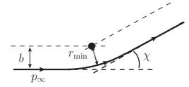
Figure 30: The scattering angle in center of mass coordinates. The black circle denotes the center of mass. The thick solid line is a schematic representation of the trajectory, with $\chi$ being the angle of deflection in the final state.

Armed with the two-body Hamiltonian, obtaining the scattering angle for two black holes (ignoring radiation effects) is straightforward. As explained in Refs. Damour:2016gwp ; Antonelli:2019ytb the scattering angle is a useful stepping stone to obtain an effective one-body Hamiltonian gr-qc/9811091 ; gr-qc/0001013 .

Before specializing to the case of our 3PM Hamiltonian, consider first the general problem of an arbitrary central-field Hamiltonian, $H({\bm{r}}^{2},{\bm{p}}^{2})$, describing the interaction of two particles in the center of mass frame. We shall assume that, as in our case, ${\bm{r}}$ and ${\bm{p}}$ are canonically-conjugate to each other. The goal is to find (an integral representation for) the scattering angle in terms of the total energy of the system and the angular momentum or, equivalently, the impact parameter.

As in the classical case of Newtonian scattering, it is convenient to use polar coordinates. As for that case, the central nature of the interaction implies that the scattering process occurs in a plane as shown in Fig. 30, so it suffices to specify only the two planar polar coordinates, ${\bm{r}}=r{\bm{e}_{r}}$ and the corresponding momenta, ${\bm{p}}=p_{r}{\bm{e}_{r}}+p_{\theta}{\bm{e}_{\theta}}$. Here ${\bm{e}_{r}}$ and ${\bm{e}_{\theta}}$ are unit vectors in the radial and angular directions, respectively. In these coordinates, Hamilton’s equations are

$$\dot{r}{\bm{e}_{r}}+r\dot{\theta}{\bm{e}_{\theta}} =2(p_{r}{\bm{e}_{r}}+p_{\theta}{\bm{e}_{\theta}})F({\bm{r}}^{2},{\bm{p}}^{2})\,,\qquad F({\bm{r}}^{2},{\bm{p}}^{2})=\frac{\partial H({\bm{r}}^{2},{\bm{p}}^{2})}{\partial{\bm{p}}^{2}}\,,$$

$$(\dot{p}_{r}-p_{\theta}\dot{\theta}){\bm{e}_{r}}+(\dot{p}_{\theta}+p_{r}\dot{\theta}){\bm{e}_{\theta}} =-2r{\bm{e}_{r}}\,K({\bm{r}}^{2},{\bm{p}}^{2})\,,\hskip 59.75095pt\;K({\bm{r}}^{2},{\bm{p}}^{2})=\frac{\partial H({\bm{r}}^{2},{\bm{p}}^{2})}{\partial{\bm{r}}^{2}}\,,\hskip 8.5359pt$$ (11.15)

and the two conservation laws are

$$J=|{\bm{r}}\times{\bm{p}}|=|{\bm{b}}\times{\bm{p}}_{\infty}|=rp_{\theta}=bp_{\infty}\,,\hskip 42.67912ptE=H(r^{2},p_{r}^{2}+p_{\theta}^{2})\,.$$ (11.16)

where $b\equiv|\bm{b}|$ is the impact parameter. We denoted the norm of the three-momentum at infinity by $p_{\infty}$; it is related to the total energy in the usual way for a scattering process,

$$E=\sqrt{p_{\infty}^{2}+m_{1}^{2}}+\sqrt{p_{\infty}^{2}+m_{2}^{2}}\,,$$ (11.17)

The two components of the first of Hamilton’s equations and the $e_{\theta}$ component of the second suffice to determine the trajectory in terms of the radial momentum $p_{r}$,

$$\frac{dr}{d\theta}=\frac{r^{2}}{J}p_{r}\,,$$ (11.18)

which in turn is determined given by conservation of energy (11.16),

$$E=H(r^{2},p_{r}^{2}+J^{2}/r^{2})\,.$$ (11.19)

We denote this solution by $p_{r}(r)$. The scattering angle is then obtained by integrating the trajectory equation (11.18):

$$\chi=-\pi+2J\int_{r_{\text{min}}}^{\infty}\frac{dr}{r^{2}\sqrt{p_{r}(r)^{2}}}\,.$$ (11.20)

We denoted the minimum distance between the two particles by $r_{\text{min}}$. At this point the radial momentum $p_{r}$ changes sign, and therefore must vanish:

$$0=p_{r}(r_{\text{min}})\,.$$ (11.21)

We shall use this relation to determine $r_{\text{min}}$.

11.3.1 Scattering Angle in the Post-Minkowskian Expansion

As discussed before, the conservative Hamiltonian for a system of two spinless compact bodies in the post-Minkowskian expansion, neglecting radiation effects, has the form (1.2)

$$H({\bm{r}}^{2},{\bm{p}}^{2})= \sqrt{{\bm{p}}^{2}+m_{1}^{2}}+\sqrt{{\bm{p}}^{2}+m_{2}^{2}}$$ (11.22)

$$+c_{1}({\bm{p}}^{2})\frac{G}{|\bm{r}|}+c_{2}({\bm{p}}^{2})\left(\frac{G}{|\bm{r}|}\right)^{2}+c_{3}({\bm{p}}^{2})\left(\frac{G}{|\bm{r}|}\right)^{3}+c_{4}({\bm{p}}^{2})\left(\frac{G}{|\bm{r}|}\right)^{4}+\dots\,.$$

The dependence on the radial coordinate is sufficiently simple to allow us to find the scattering angle for arbitrary coefficients $c_{i}({\bm{p}}^{2})$, whose index reflects the PM order at which they appear. Since this structure of the Hamiltonian relies only on the spinless nature of the particles and Lorentz invariance of their interactions, such a general expression can also be used to explore extensions of General Relativity by further fields and/or further interactions.

The radial momentum $p_{r}$ as a function of the radial coordinate $r\equiv|\bm{r}|$, obtained by solving perturbatively (11.19), is

$$p^{2}_{r}(r)=\frac{p_{\infty}^{2}r^{2}-J^{2}}{r^{2}}+P_{1}\frac{G}{r}+P_{2}\left(\frac{G}{r}\right)^{2}+P_{3}\left(\frac{G}{r}\right)^{3}+P_{4}\left(\frac{G}{r}\right)^{4}+{\cal O}(G^{5})\,.$$ (11.23)

The coefficients $P_{i}$ will be listed shortly. The vanishing of $p_{r}(r)$ determines the minimum distance $r_{\text{min}}$:

$$r_{\text{min}}^{2}=\hbox{} b^{2}-b^{3}P_{1}\frac{G}{J^{2}}+\frac{b^{4}}{2}(P_{1}^{2}-2p_{\infty}^{2}P_{2})\frac{G^{2}}{J^{4}}$$ (11.24)

$$-\frac{b^{5}}{8}(P_{1}^{3}-4p_{\infty}^{2}P_{1}P_{2}+8p_{\infty}^{4}P_{3})\frac{G^{3}}{J^{6}}-b^{6}p_{\infty}^{6}P_{4}\frac{G^{4}}{J^{8}}+{\cal O}(G^{5})\,.$$ (11.25)

Using Eqs. (11.23) and (11.25) in Eq. (11.20), it is not difficult to find the scattering angle through fourth order in the PM expansion , in terms of the expansion coefficients in Eq. (11.23)

$$\chi=\sum_{i\geq 1}\chi^{i\text{PM}}= \frac{P_{1}}{p_{\infty}}\left(\frac{G}{J}\right)+\frac{\pi}{2}P_{2}\left(\frac{G}{J}\right)^{2}-\frac{P_{1}^{3}-12p_{\infty}^{2}P_{1}P_{2}-24p_{\infty}^{4}P_{3}}{12p_{\infty}^{3}}\left(\frac{G}{J}\right)^{3}$$

$$\hbox{}+\frac{3\pi}{8}(P_{2}^{2}+2P_{1}P_{3}+2p_{\infty}^{2}P_{4})\left(\frac{G}{J}\right)^{4}+{\cal O}\left((G/J)^{5}\right)\,,$$ (11.26)

where the $\chi^{i\text{PM}}$ is the angle at the order $(G/J)^{i}$. The dependence on the momentum at infinity may be traded for dependence on the total energy by inverting Eq. (11.17):

$$p_{\infty}^{2}=\frac{1}{4E^{2}}(E^{2}-(m_{1}-m_{2})^{2})(E^{2}-(m_{1}+m_{2})^{2})\,.$$ (11.27)

Lastly, the coefficients $P_{i}$ of the $G$ expansion of the radial momentum are:

$$P_{1}=\hbox{} -2E\xi{\bar{c}}{}_{1}\,,$$ (11.28)

$$P_{2}=\hbox{} -2E\xi{\bar{c}}{}_{2}+(1-3\xi){\bar{c}}{}_{1}^{2}+4E^{2}\xi^{2}{\bar{c}}{}_{1}{\bar{c}}^{\prime}{}_{1}\,,$$ (11.29)

$$P_{3}=\hbox{} -2E\xi{\bar{c}}{}_{3}+2(1-3\xi){\bar{c}}{}_{1}{\bar{c}}{}_{2}-4E^{3}\xi^{3}{\bar{c}}{}_{1}\left(2{\bar{c}}^{\prime}{}_{1}^{2}+{\bar{c}}{}_{1}{\bar{c}}^{\prime\prime}{}_{1}\right)+4E^{2}\xi^{2}\left({\bar{c}}{}_{2}{\bar{c}}^{\prime}{}_{1}+{\bar{c}}{}_{1}{\bar{c}}^{\prime}{}_{2}\right)$$

$$-6E(1-3\xi)\xi{\bar{c}}{}_{1}^{2}{\bar{c}}^{\prime}{}_{1}+\frac{(1-4\xi){\bar{c}}{}_{1}^{3}}{E}\,,$$ (11.30)

$$P_{4}=\hbox{} -2E\xi{\bar{c}}{}_{4}+\frac{8}{3}E^{4}\xi^{4}{\bar{c}}{}_{1}\left(6{\bar{c}}^{\prime}{}_{1}^{3}+9{\bar{c}}{}_{1}{\bar{c}}^{\prime\prime}{}_{1}{\bar{c}}^{\prime}{}_{1}+{\bar{c}}{}_{1}^{2}{\bar{c}}^{\prime\prime\prime}{}_{1}\right)+\frac{5(1-4\xi){\bar{c}}{}_{1}^{4}}{4E^{2}}+\frac{3(1-4\xi){\bar{c}}{}_{1}^{2}{\bar{c}}{}_{2}}{E}\hskip 56.9055pt$$

$$-4E^{3}\xi^{3}\left(2{\bar{c}}{}_{2}\left({\bar{c}}^{\prime}{}_{1}^{2}+{\bar{c}}{}_{1}{\bar{c}}^{\prime\prime}{}_{1}\right)+{\bar{c}}{}_{1}\left(4{\bar{c}}^{\prime}{}_{1}{\bar{c}}^{\prime}{}_{2}+{\bar{c}}{}_{1}{\bar{c}}^{\prime\prime}{}_{2}\right)\right)+(1-3\xi){\bar{c}}{}_{2}^{2}$$

$$+4E^{2}\xi^{2}\left(2(1-3\xi){\bar{c}}^{\prime\prime}{}_{1}{\bar{c}}{}_{1}^{3}+6(1-3\xi){\bar{c}}^{\prime}{}_{1}^{2}{\bar{c}}{}_{1}^{2}+{\bar{c}}^{\prime}{}_{3}{\bar{c}}{}_{1}+{\bar{c}}{}_{3}{\bar{c}}^{\prime}{}_{1}+{\bar{c}}{}_{2}{\bar{c}}^{\prime}{}_{2}\right)$$

$$-6E(1-3\xi)\xi{\bar{c}}{}_{1}\left(2{\bar{c}}{}_{2}{\bar{c}}^{\prime}{}_{1}+{\bar{c}}{}_{1}{\bar{c}}^{\prime}{}_{2}\right)+2{\bar{c}}{}_{1}\left((1-5\xi)^{2}{\bar{c}}^{\prime}{}_{1}{\bar{c}}{}_{1}^{2}+(1-3\xi){\bar{c}}{}_{3}\right)\,,$$ (11.31)

where ${\bar{c}}_{i}\equiv c_{i}(p_{\infty}^{2})$, the primes denote derivatives with respect to the argument and, as before, $E=E_{1}+E_{2}$ and $\xi=E_{1}E_{2}/E^{2}$. The $c_{i}$ are the coefficients in the potential in Eq. (10.8) and are given in Eq. (10.10). The expressions relating $P_{i\geq 5}$ to the coefficients of the Hamiltonian are lengthier, but may be derived without difficulty by inverting Eq. (11.16), iteratively in Newton’s constant.

We note that all coefficients $P_{i}$ have the structure

$$P_{i}=-2E\xi{\bar{c}}_{i}+\dots\,,$$ (11.32)

where the ellipsis only depend on Hamiltonian coefficients $c_{j}$ with $j<i$ and their derivatives; this may be easily understood from the special structure of the Hamiltonian (11.22). We also note that there exists a close relation between the coefficients $P_{i}$ and the EFT amplitudes at the same order in $G$. Indeed, comparing eqs. (11.28), (11.29) and (11.30) with (10.6) it is easy to see that $P_{i}$ is proportional to the IR-finite part of the EFT amplitudes. We expect that this feature will continue to higher PM orders.

11.3.2 Angle Through 3PM and Comparison with Known Results

Using (11.28), (11.29), (11.30) and (11.26) as well as the Hamiltonian (10.8)-(10.10), it is straightforward to obtain that, through 3PM order, the conservative part of the scattering angle is 3PMPRL ; Antonelli:2019ytb

$$\chi^{\text{1PM}} \hbox{}=\frac{2(2\sigma^{2}-1)}{\sqrt{\sigma^{2}-1}}\frac{\nu m^{2}G}{J}\,,$$

$$\chi^{\text{2PM}} \hbox{}=\frac{3\pi}{4}\frac{5\sigma^{2}-1}{\sqrt{1+2\nu(\sigma-1)}}\frac{\nu^{2}m^{4}G^{2}}{J^{2}}\,,$$

$$\chi^{\text{3PM}} \hbox{}=-\biggl{[}\frac{1}{12}\left(\frac{2(2\sigma^{2}-1)}{\sqrt{\sigma^{2}-1}}\right)^{3}-\frac{2}{\pi}\left(\frac{2(2\sigma^{2}-1)}{\sqrt{\sigma^{2}-1}}\right)\biggl{(}\frac{3\pi}{4}\frac{5\sigma^{2}-1}{\sqrt{1+2\nu(\sigma-1)}}\biggr{)}$$

$$+4\,\frac{\sqrt{\sigma^{2}-1}}{2(\sigma-1)\nu+1}\biggl{(}-\frac{3\nu\left(1-5\sigma^{2}\right)\left(1-2\sigma^{2}\right)(2\nu(\sigma-1)+1)}{2(\sigma+1)\left(2\nu(\sigma-1)+\sqrt{2\nu(\sigma-1)+1}+1\right)}$$ (11.33)

$$\qquad\qquad-\frac{4\nu\left(-4\sigma^{4}+12\sigma^{2}+3\right)}{\sqrt{\sigma^{2}-1}}\,{\rm arcsinh}\!\left(\frac{\sqrt{\sigma-1}}{\sqrt{2}}\right)$$ (11.34)

$$\qquad\qquad+\frac{1}{12}\left(4\nu\sigma^{3}+108\nu\sigma^{2}+206\nu\sigma-54\sigma^{2}-6\nu+3\right)\biggl{)}\biggr{]}\frac{\nu^{3}m^{6}G^{3}}{J^{3}}\,.\hskip 56.9055pt$$ (11.35)

Using the observation that $P_{i}$ are proportional to the IR-finite parts ${\cal M}^{\prime}_{i}$ of the EFT amplitudes evaluated at $p=p_{\infty}$, the angle can be rewritten very compactly as 3PMPRL

$$2\pi\chi={d_{1}\over J}+{d_{2}\over J^{2}}+\frac{1}{J^{3}}\biggl{(}\vphantom{\frac{1}{\pi^{2}}}{-4d_{3}}+{d_{1}d_{2}\over\pi^{2}}-{d_{1}^{3}\over 48\pi^{2}}\biggr{)}\,,$$ (11.36)

where $d_{i}$ are defined in terms of ${\cal M}^{\prime}_{i}$ as

$$d_{1}=m\gamma\xi{\bm{q}}^{2}{\cal M}_{1}^{\prime}/|{\bm{p}}|\,,\hskip 28.45274ptd_{2}=m\gamma\xi|\bm{q}|{\cal M}_{2}^{\prime}\,,\hskip 28.45274ptd_{3}=m\gamma\xi|{\bm{p}}|{\cal M}_{3}^{\prime}/\ln{\bm{q}}^{2}\,,$$ (11.37)

and $p\rightarrow p_{\infty}$ is implicitly understood.

The 2PM angle has been obtained through a variety of methods in Refs. Damour:2016gwp ; DamourTwoLoop ; BjerrumClassical ; Cristofoli:2019neg , and our result is in agreement. Moreover, the 4PN terms in the 3PM angle reproduce the corresponding terms in Bini:2017wfr . This is, of course, to be expected since we have already shown that the 4PN part of our Hamiltonian reproduces (up to a canonical transformation) the ${\cal O}(G^{3})$ part of the known 4PN Hamiltonian.

One may parametrize the higher-PM angle in several different ways; given the expected relation between the $P_{i}$ coefficients in Eq. (11.23) and the classical limit of the IR-finite parts of the $i$-loop amplitude, it seems convenient to parameterize them recursively in terms of the lower-PM angle and $P_{i}$. For example, the 4PM angle without radiation effect can be written as:

$$\chi^{\text{4PM}} \hbox{}=\frac{3\pi p_{\infty}^{2}G^{4}}{4J^{4}}P_{4}+\frac{3\pi}{8}\chi^{\text{1PM}}\chi^{\text{3PM}}+\frac{3}{2\pi}(\chi^{\text{2PM}})^{2}-\frac{3}{4}(\chi^{\text{1PM}})^{2}\chi^{\text{2PM}}+\frac{\pi}{32}(\chi^{\text{1PM}})^{4}\,.$$ (11.38)

It would be interesting to understand the relation between the method used here to compute the scattering angle and the one based on the eikonal limit of scattering amplitudes StermanEikonal . In particular, it would be interesting to see how terms proportional to the IR-finite part of scattering amplitudes (11.36) arise from the recent amplitude-based methods OConnellObservables ; BjerrumClassical ; Cristofoli:2019neg .

12 Discussion

In this section we discuss various features and subtleties in our results. In particular, we describe the mass singularity that appears in our 3PM results, as well as subtleties associated with infrared singularities. In general relativity infrared singularities are quite tame compared to gauge theory, because they are a simple exponential of one-loop divergence Weinberg:1965nx ; 1101.1524 ; Akhoury:2011kq . We therefore do not anticipate serious difficulties at higher loops when applying four-dimensional methods to construct integrands relevant for extracting classical physics. In this section we analyze the one- and two-loop situations, to show that straightforward application of four-dimensional helicity methods indeed gives the same final result as a more careful treatment, where all steps are computed in $D=4-2\epsilon$ dimensions, as required when using conventional dimensional regularization.

We also comment on radiative contributions to conservative dynamics, which we show are not relevant at 3PM order, but should become important at the next order in the post-Minkowskian approximation.

12.1 Mass Singularities and Collinear Structure

A feature of the 3PM amplitude (9.3), Hamiltonian (10.8) and scattering angle (11.36) is that as both masses are taken to vanish a logarithmic mass singularity develops, as displayed in Eq. (9.6). At first sight this might seem surprising because quantum amplitudes do not have mass or, equivalently, collinear singularities Weinberg:1965nx ; 1101.1524 ; Akhoury:2011kq . Since our results originate from a quantum amplitude, one might be surprised by its appearance in our final results.

In this section we trace the origin of the mass singularity as due to an inability to interchange the classical and massless limits originating from our hierarchy of scales (2.5), that takes the momentum transfer $|\bm{q}|\ll m_{i}$, while assuming that both masses $m_{i}$ have fixed finite values.

As explained in Sec. 2, we defined the PM potential such that, at each order in Newton’s constant, its velocity expansion matches all corresponding terms in the PN expansion. Indeed, as discussed in Sec. 11, the known 4PN Hamiltonian JaranowskSchafer1 ; JaranowskSchafer2 confirms the first three terms of the small-velocity expansion of the arcsinh term which becomes logarithmically-divergent in the massless limit. One may attempt to define a Hamiltonian for which the limit is smooth by e.g. resumming the various logarithmic terms to all orders in $G$ expansion, but, given the above, it is unclear how such a result would match known PN potentials, without introducing extraneous contributions. Of course, a function that is smooth in the massless limit and contains all information necessary for constructing the classical potential is the full quantum amplitude. However, this function is likely highly nontrivial to construct and manipulate.

We verified that it is not possible to remove this mass singularity of the classical potential by a canonical transformation, which is consistent with it appearing also in the amplitude and in the scattering angle. This implies that the massless limit is generally discontinuous—and in fact may be ill-defined if taken after arriving at the classical potential. On the other hand, if the massless limit, is taken prior to taking the classical limit we do expect to smoothly match onto other purely massless computations, such as the scattering angle in the high-energy limit obtained via eikonal methods in Ref. ACV .

From an intuitive perspective, it is perhaps not so surprising that the massless limit is subtle. After all, we usually think of a potential as mediating an instantaneous force between two bodies. We naturally expand the potential about the static limit in which the relative velocity is zero. However, if interacting particles are moving at the speed of light, this notion of instantaneous potential becomes unclear.

Our non-relativistic integration methods explicitly assume, following the construction of the classical limit in Sec. 2, that the momentum transfer is much smaller than the mass in order to define potential-mode gravitons. Although, not relying on a velocity expansion, when using relativistic methods for evaluating the integrals in Sec. 8 we make a similar assumption, by first carrying out the asymptotic expansion at small-momentum transfer. Once the integration is carried out, one naturally expects to encounter difficulties when attempting to interchange the order of limits and compare the result with one obtained in a massless theory. Similar interchange of limits issues appear, for example, in factorization limits of infrared divergent theories Bern:1995ix . Indeed, the massless limit of our results at two loops, included in Eq. (9.6) does not match those of Ref. ACV , obtained in the high energy limit.

In order to sharpen our understanding of the mass singularity appearing in our results, we analyze its appearance in the case in the first subleading quantum terms in the small-$q$ expansion of the one-loop amplitude, as noted in Refs. PierreLogM ; Paolo2PM . We will do so as follows:

• We explicitly confirm the well-known cancellation of mass singularities in the full one-loop quantum amplitude.

• We explicitly show that the small-$q$ limit does not commute with the massless limit for the first quantum correction to the amplitude.

Our conclusion will be that the 3PM classical potential indeed has a discontinuity in the $m\rightarrow 0$ limit.

We note that while the mass singularity is not of phenomenological interest in the inspiral region because the logarithm is of order unity, it is of some theoretical interest to understand its origin and, even better, to attempt to exploit it. Typically, mass singularities in gauge theories can be resummed to all orders in the coupling. This could conceivably form the basis of new approximation schemes. In any case, in this section, we explain the appearance of a mass singularity within our framework.

12.1.1 Absence of Mass Singularity for $\bm{q}^{2}\gg m^{2}$

A full analysis of the mass singularity at two-loop case is nontrivial, in part, because of the difficulty of carrying out the loop integration without making explicit use of the classical limit. We therefore instead carry out a detailed one-loop analysis. This offers important insight, because it also exhibits a similar mass singularity, albeit starting in the first subleading quantum contribution PierreLogM ; Paolo2PM . The complete one-loop quantum amplitude is straightforward to evaluate, allowing us to track both the cancellation of the mass singularities in the full quantum theory Akhoury:2011kq and to track how these cancellations break down when expanding around the classical limit. The result is that the expansion around the classical limit does not commute with the small-mass limit.

We first show that, for fixed kinematical invariants $s$ and $t$, the one-loop quantum amplitude does not contain a $\ln(m_{1}m_{2})$ singularity for small $m_{1}$ and $m_{2}$, as expected. While modern methods can help BCJ ; GeneralizedDoubleCopy , we used Feynman diagrams since this calculation is simple enough, followed by standard loop integration methods Chetyrkin:1981qh ; Laporta:2001dd . In carrying out this computation, we ignore bubble-on-external-leg contributions, since these do not carry the mass singularities: such contributions are suppressed by factors of mass-squared, as follows from simple dimensional analysis and the fact that the only kinematic invariant they can depend on is $p_{i}^{2}=m_{i}^{2}$. Because the calculation of the integrand and its integration is straightforward, we do not include the details here, but merely quote the result focusing on collinear and mass singularities.

For one-loop calculations, it is possible to organize the amplitude as linear combinations of scalar “master” integrals. Our results is given by

$$\mathcal{M}{}^{(1)}=\sum_{i=1}^{17}a_{i}\,I^{(1)}_{i}\,,$$ (12.1)

where $I^{(1)}_{i}$ is the master integral of the one-loop graph $i$ in Table 3. The master integral is defined as

$$I^{(1)}_{i}=\int d^{D}\ell\,\frac{e^{\gamma_{E}\epsilon}}{i\pi^{D/2}}\,\frac{1}{\prod_{j\in i}D_{j}}\,,$$ (12.2)

where $\prod_{j}D_{j}$ is the product of all inverse propagators corresponding to the edges of the graph $i$ in Table 3, and $\gamma_{E}$ is the Euler constant. The coefficients $a_{i}$ in Eq. (12.1) depend on external masses and Mandelstam invariants. A property that will be useful shortly is that all coefficients are regular in the small $m_{1}$ and $m_{2}$ limit.

Table 3: Master integrals $I^{(1)}_{1}$ to $I^{(1)}_{9}$ for the one-loop scattering amplitude in the full quantum theory. The thin lines are massless and thick lines are massive. The internal masses are specified explicitly. The other master integrals are obtained from the displayed one via relabeling. The $u$-channel integrals, $I^{(1)}_{10,11,12}$, are given by $I^{(1)}_{2,6,9}$ with $2\leftrightarrow 3$. The master integrals $I^{(1)}_{13,14,15,16,17}$ are obtained from $I^{(1)}_{1,4,5,7,8}$ by the map $(1,4)\leftrightarrow(2,3)$ as well as exchanging internal masses $m_{1}\leftrightarrow m_{2}$.

All the analytic expressions of the scalar tadpole, bubble, triangle, and box integrals can be found in Ref. Ellis:2007qk . We derive their small-mass logarithmic singularities using the Mellin-Barnes method briefly reviewed in Sec. 8.2 and implemented in the computer codes MB.m and MBasymptotics.m; the resulting expressions are, of course, consistent with the integrals listed in Ref. Ellis:2007qk . Integrals $I^{(1)}_{1},I^{(1)}_{2},I^{(1)}_{3},I^{(1)}_{4},I^{(1)}_{10},I^{(1)}_{13}$ and $I^{(1)}_{14}$ are smooth when $m_{i}\rightarrow 0$. $I^{(1)}_{1}$ and $I^{(1)}_{13}$ in fact vanish in this limit, being proportional to $m_{i}^{2}$. The other five bubble integrals are also regular in the massless limit, because in this limit the total momentum flowing through them is fixed and nonzero. An important property of all 17 integrals is that they do not exhibit any power-like singularities in the small-mass limit with fixed momentum transfer.

The singular terms as $m_{i}\rightarrow 0$ for the remaining ten integrals are collected in the third column of Table 4. Since none of them exhibits a power-like mass singularity to study the $\ln m_{i}$ behavior of the amplitude it is sufficient to evaluate the integral coefficients with vanishing masses. These coefficients are collected in the second column of Table 4.

$i$	$a_{i}$	$I^{(1)}_{i}$
$5$	$0$	$\displaystyle{\frac{1}{\epsilon}+2-2\ln m_{1}}$
$6$	$\frac{\pi^{2}s^{3}}{8}$	$\displaystyle{\frac{1}{\epsilon\,s}\,\left(\ln m_{1}+\ln m_{2}\right)-\frac{1}{s}\left((\ln m_{1})^{2}+(\ln m_{2})^{2}\right)+\dotsc}$
$7$	$\frac{1}{16}\pi^{2}t(s^{2}-su+u^{2})$	$\displaystyle{\frac{2}{t}\left((\ln m_{1})^{2}-\ln(-t)\ln m_{1}\right)+\dotsc}$
$8$	$-\frac{1}{16}\pi^{2}stu$	$\displaystyle{\frac{2}{t}\left(\frac{1}{\epsilon}\ln m_{1}-(\ln m_{1})^{2}\right)+\dotsc}$
$9$	$\frac{1}{16}\pi^{2}s^{4}$	$\displaystyle{\frac{2}{st}\left(\frac{1}{\epsilon}-\ln(-t))\right)(\ln m_{1}+\ln m_{2})+\dotsc}$
$11$	$\frac{1}{8}\pi^{2}u^{3}$	$\displaystyle{I^{(1)}_{6}\Big{|}_{(2\leftrightarrow 3)}}$
$12$	$\frac{1}{16}\pi^{2}u^{4}$	$\displaystyle{I^{(1)}_{9}\Big{|}_{(2\leftrightarrow 3)}}$
$15$	$0$	$\displaystyle{I^{(1)}_{5}\Big{|}_{((1,4)\leftrightarrow(2,3);m_{1}\leftrightarrow m_{2})}}$
$16$	$\frac{1}{16}\pi^{2}t(s^{2}-su+u^{2})$	$\displaystyle{I^{(1)}_{7}\Big{|}_{((1,4)\leftrightarrow(2,3);m_{1}\leftrightarrow m_{2})}}$
$17$	$-\frac{1}{16}\pi^{2}stu$	$\displaystyle{I^{(1)}_{8}\Big{|}_{((1,4)\leftrightarrow(2,3);m_{1}\leftrightarrow m_{2})}}$

Table 4: Master integrals in the physical region and their coefficients in the small-mass limit. Integrals not included explicitly do not have any $\ln m_{i}$ singularities. Ellipsis contain terms which are regular in the small-mass limit but may contain divergence in the dimensional regulator $\epsilon$.

It is not difficult to see that by multiplying the second and third column and adding the resulting ten terms all the simple and double mass logarithms cancel out, as required by the general argument of Ref. Akhoury:2011kq . For example, the complete soft and collinearly-divergent terms in the sum of integrals $I^{(1)}_{6}$ and $I^{(1)}_{11}$, proportional to $(s^{2}+u^{2})\ln(m_{1}m_{2})/\epsilon$, cancel against similar terms in the sum of integrals $I^{(1)}_{9}$ and $I^{(1)}_{12}$. The remainder, proportional to $su\ln(m_{1}m_{2})/\epsilon$, cancels against analogous terms in the sum of $I^{(1)}_{8}$ and $I^{(1)}_{17}$. Relations between Mandelstam invariants are, of course, essential. A second cancellation that is easy to see by inspection is that of the double logarithms $\ln(-t)\ln(m_{1}m_{2})$, which are given only by $I^{(1)}_{7}+I^{(1)}_{16},I^{(1)}_{9}$ and $I^{(1)}_{12}$. The first combination of integrals gives the double logarithms under discussion while the sum of the second integrals, each of which has the double logarithms, produces the necessary overall coefficient.

All integrals in Table 4 are essential for the complete cancellation of collinear singularities. However, not all of them survive in the small-$q$ limit. This can be seen by examining the $t$-dependence of the combination of the integrals and their coefficients which needs to yield $t^{-1/2}$ or $\ln(-t)$ dependence to contribute to the classical 2PM potential or the first quantum correction to it, respectively. For example, the combination $a_{6}I^{(1)}_{6}$ does not appear in the construction of 2PM potential, either at the classical and the first quantum order, because it only depends on the $s$ Mandelstam invariant.

12.1.2 Appearance of Mass Singularity for $\bm{q}^{2}\ll m^{2}$

Now that we understand in detail how the mass singularity cancels in the complete one-loop quantum amplitude, we can explore the breakdown of this cancellation when expanding around the classical limit. As noted in Refs. PierreLogM ; Paolo2PM , while there is no mass singularity in the 2PM amplitude used to derive the classical potential, there is one in the first subleading quantum correction to it. This provides a much simpler case to study than at two loops, which nonetheless has similar features. We will first identify the mass singularity and recall how it cancels in the quantum theory, and then proceed to show that it no longer does if the amplitude is first series-expanded in small $|\bm{q}|$ to extract the classical potential.

In Ref. Paolo2PM , the first quantum correction to the classical potential is shown to have a $\ln(m_{1}m_{2}/s)$ singularity. It originates from the one-loop scalar box integral $I^{(1)}_{9}$ in Table 3, which has no classical limit. Interestingly, the same type of function appears at two loops. The complete expression of the box integral with two internal massive lines is Beenakker:1988jr ; Smirnov:2004ym ; Ellis:2007qk

$$I^{(1)}_{9}=\frac{2}{t\sqrt{(s-\Delta m^{2})(s-M^{2})}}\left(\frac{1}{\epsilon}-\ln\left(\frac{-t}{\mu^{2}}\right)\right)\Biggl{(}\ln\Biggl{(}\frac{1-\sqrt{\frac{s-M^{2}}{s-\Delta m^{2}}}}{1+\sqrt{\frac{s-M^{2}}{s-\Delta m^{2}}}}\,\Biggr{)}+i\pi\Biggr{)}\,,$$ (12.3)

where $\Delta m^{2}=(m_{1}-m_{2})^{2}$ and $M^{2}=(m_{1}+m_{2})^{2}$. The dependence on $t=-|\bm{q}|^{2}$ and on mass are factorized, so the small-$t$ expansion and the massless limits commute trivially. However, this integral exhibits a logarithmic singularity in the small-mass limit

$$I^{(1)}_{9}=\frac{2}{t\,s}\left(\frac{1}{\epsilon}-\ln(-t)\right)\ln\left(\frac{m_{1}m_{2}}{s}\right)+\dotsc\,,$$ (12.4)

where the ellipsis stand for a power series in $m_{i}m_{j}/s$. Combining this with the cross-box integral, $I^{(1)}_{12}$, obtained by the replacement $s\rightarrow u=-s-t+M^{2}+\Delta m^{2}$, and using the integral coefficients $a_{9}$ and $a_{12}$ in Table 4 exposes the complete mass singularity of the first subleading quantum correction to the amplitude:

$$a_{9}I^{(1)}_{9}+a_{12}I^{(1)}_{12}=-\frac{\pi^{2}}{8}(s^{2}-su+u^{2})\left(\frac{1}{\epsilon}-\ln(-t)\right)\ln\left(\frac{m_{1}m_{2}}{s}\right)+\dotsc\,,$$ (12.5)

where the ellipsis contain terms that are regular in the small-$m_{i}$ limit as well as higher orders in a small-$t$ expansion. This reproduces the mass singularity as found in Ref. Paolo2PM in the leading quantum correction to the 2PM amplitude.

As discussed above in Sec. 12.1.1, in the small-mass limit taken at fixed $t$ and $s$, the overlap of soft and collinear singularities in the contribution of $I^{(1)}_{9}$ and $I^{(1)}_{12}$, $\ln(m_{1}m_{2})/\epsilon$, cancels against the sum of $I^{(1)}_{6},I^{(1)}_{11},I^{(1)}_{8}$ and $I^{(1)}_{17}$, while the double logarithm, $\ln(-t)\ln(m_{1}m_{2})$, cancels against the sum of $I^{(1)}_{7}$ and $I^{(1)}_{16}$. Thus, to understand the fate of collinear singularities in an expansion around the classical limit it suffices to expand these integrals first at small $t$ and then at small $m_{i}$. Using MB.m and MBasymptotics.m one finds that $I^{(1)}_{6}$ and $I^{(1)}_{11}$ are given by the same expressions in Table 4. The other four integrals are different. $I^{(1)}_{7}$ and $I^{(1)}_{8}$ are given by

$$\bigl{(}I^{(1)}_{7}\bigr{|}_{t\to 0}\bigr{)}\bigr{|}_{m_{i}\to 0} = -\frac{\pi^{2}}{2m_{1}\sqrt{-t}}-\frac{1}{2m_{1}^{2}}\left(\ln(-t)-2\ln m_{1}-2\right)+\dotsc$$ (12.6)

$$\bigl{(}I^{(1)}_{8}\bigr{|}_{t\to 0}\bigr{)}\bigr{|}_{m_{i}\to 0} = \frac{1}{2m^{2}_{1}}\left(\frac{1}{\epsilon}-2\ln m_{1}\right)+\dotsc\,,$$ (12.7)

and $I^{(1)}_{16}$ and $I^{(1)}_{17}$ are given by the appropriate relabelings. The ellipsis stand for terms which are regular in the limit $t\rightarrow 0,|t|\ll m^{2}_{i}$ and $s$ fixed; on dimensional grounds all these terms are increasingly more singular as $m_{i}\rightarrow 0$. Comparing with the relevant entries in Table 4 we see that $I^{(1)}_{7},I^{(1)}_{8},I^{(1)}_{16}$ and $I^{(1)}_{17}$ have different expansions around the small-mass limit and around the classical limit. In particular, in the later expansion they contain stronger-than-logarithmic singularities in the mass while missing the soft-collinear overlap, $\ln m_{i}/\epsilon$, and double-logarithms $\ln(-t)\ln m_{i}$. It is therefore clear that the cancellation of collinear singularities in the small-mass expansion is broken in the expansion around the classical limit. Thus, the small-$m$ and small-$t$ expansions do not commute. Because the $1/t$ appearing in the small-mass limit is replaced by a $1/m_{1}^{2}$ in the small $t$ limit, the contributions from $I^{(1)}_{7}$ and $I^{(1)}_{8}$, and their coefficients in the expansion around the classical result are subsubleading in the expansion around the classical limit and thus unable to cancel the mass singularity (12.5) appearing in the first subleading quantum correction.

The expansions (12.7) may be confirmed by starting from the known analytic expressions for $I^{(1)}_{7}$ and $I^{(1)}_{8}$ in the physical $t<0$ region; for example, the latter integral is given by Ellis:2007qk :

$$I^{(1)}_{8}=\frac{x_{t}}{m_{1}^{2}\,(1-x_{t}^{2})}\left[\ln x_{t}\left(-\frac{1}{\epsilon}-\frac{1}{2}\ln x_{t}+2\ln(1-x_{t}^{2})+\ln\frac{m_{1}^{2}}{\mu^{2}}\right)-\frac{\pi^{2}}{6}+\textrm{Li}_{2}(x_{t}^{2})+2\textrm{Li}_{2}(1-x_{t})\right],$$ (12.8)

where $\mu$ is the dimensional regularization scale and

$$x_{t}=\frac{-t}{4m_{1}^{2}}\left(\sqrt{1+\frac{4m_{1}^{2}}{-t}}-1\right)^{2}.$$ (12.9)

While we have not carried out the corresponding calculation at two loops, the one-loop calculation described in detail here illustrates that, generically, the small-$m$ and small-$t$ expansions do not commute and moreover that the latter expansion contains remnants of collinearly-singular terms that cancel in the former, in agreement with the general arguments of Ref. Akhoury:2011kq . Based on our one-loop analysis, we therefore conclude that mass singularities in the 3PM classical potential are not surprising.

12.2 Four- vs. $D$-Dimensional Integrands

An important issue which can help streamline future calculations is whether we can compute the integrand for the classical potential using only four-dimensional methods or whether it is necessary to be more careful and use $D$-dimensional methods when dimensionally regularizing infrared singularities.

When using four-dimensional helicity methods to construct the integrand the following choices are implicitly made:

1. Terms containing Gram determinants or terms that vanish in four but not in $D$ dimensions are not included. Equivalently, terms containing loop momenta that are outside the four-dimensional subspace are dropped.

2. The state-counting parameter is implicitly taken to be $D_{s}=4$.

This is to be contrasted to conventional dimensional regularization which keeps all such Gram determinants, and takes $D_{s}=4-2\epsilon$. Here we show that through two loops these differences in prescription have no effect on the final classical potential. Some points which appear to be generic underlie this conclusion:

• Terms with $(-2\epsilon)$-dimensional components of loop momentum are suppressed in $\epsilon$ and cannot contribute unless they interfere with $1/\epsilon$ singularities. However, after extracting an explicit factor of $\epsilon$, it turns out that remaining integrals are equivalent to integrals in higher dimensions that cannot be infrared singular. If a contribution remains it must come from an ultraviolet divergence whose origin is quantum mechanical.

• The dependence on the state-counting $D_{s}$ parameter may strike infrared singularities and thus modify the integrand by finite terms. However, even if some terms were to remain, the $D_{s}$ prescription needs to be applied consistently and uniformly to different orders in the PM expansion, including in the EFT. The net effect is that the iteration terms in the EFT should automatically subtract any prescription differences.

• The $(-2\epsilon)$-dimensional terms, whether from $D_{s}$ or $(-2\epsilon)$-dimensional components of loop momenta, are of the wrong form to generate classical contributions. In particular, at 3PM order they do not generate the required $\ln{\bm{q}}^{2}$ terms.

While a detailed proof beyond 3PM order is beyond the scope of this paper, the fact that the underlying ideas appear to be generic suggests that helicity methods will also be sufficient at higher orders.

12.2.1 Integrand Comparison at One Loop

Before turning to the 3PM case, it is useful to understand how four-dimensional helicity methods for constructing the integrand lead to the correct 2PM potential. As emphasized earlier, at first sight one might worry that, in the presence of ${\cal O}(1/\epsilon)$ infrared singularities, terms of ${\cal O}(\epsilon)$ originating from differences between four- and $D$-dimensional methods may yield errors in finite terms. We will show that this does not happen.

As already noted in Sec. 5, there are only four independent momenta in the one-loop integrand: three external and one loop momentum. Thus, it is not possible to form a Gram determinant that vanishes in four dimensions but not in general dimensions. Consequently, four-dimensional helicity methods must fully reconstruct the $D$-dimensional integrand, up to the choice of the $D_{s}$ parameter, which four-dimensional helicity methods implicitly fix to $D_{s}=4$. This reduces the question of whether the classical potential obtained through helicity methods drops any important terms to that of whether we can use $D_{s}=4$ in the simplified physical state projector in Eq. (5.20) without affecting the potential.

As we discussed in Sec. 10, the triangle integrals are infrared-finite and the only infrared divergence comes from box integrals. Thus, only their contribution is sensitive to the value of $D_{s}$. The part of the box-integral coefficient proportional to $(D_{s}-4)$ can be obtained from Eq. (5.22) by cutting the $i/\tau_{15}$ propagator, so that all four box propagators are cut. Combining this with the $D_{s}=4$ result (4.39), gives the $D_{s}$-dependent coefficient of the box integral

$$C_{\rm box}= ((s-m_{1}^{2}+m_{2}^{2})^{2}-2m_{1}^{2}m_{2}^{2})^{2}+\frac{4m_{1}^{2}m_{2}^{2}(D_{s}-4)}{(D_{s}-2)}\Big{(}(s-m_{1}^{2}-m_{2}^{2})^{2}-m_{1}^{2}m_{2}^{2}\frac{D_{s}}{D_{s}-2}\Bigr{)}$$

$$= \left((s-m_{1}^{2}-m_{2}^{2})^{2}-\frac{4}{D_{s}-2}m_{1}^{2}m_{2}^{2}\right)^{2}.$$ (12.10)

Its essential property is that it is the square of the numerator of the tree amplitude in $D_{s}$ dimensions,

$$M_{4}(1^{s},2^{s},3^{s},4^{s})=\frac{i}{t}\Bigl{(}(s-m_{1}^{2}-m_{2}^{2})^{2}-\frac{4}{D_{s}-2}m_{1}^{2}m_{2}^{2}\Bigr{)}\,.$$ (12.11)

That is, the only modification that survives as $\epsilon\rightarrow 0$ is that the coefficient of the four-dimensional box integral (4.39) is the $D_{s}$-dimensional tree amplitude instead of the four-dimensional one. Because the box contains the only infrared singularity of the one-loop amplitude which, by construction, is the same as that of the EFT, it follows that the complete $D_{s}$ dependence of the one-loop amplitude is reproduced by the iterated $D_{s}$-dependent tree amplitude of the EFT. The net effect is that, when the iterated tree including $D_{s}$ dependence is subtracted to determine the 2PM potential, the $D_{s}$ dependence is subtracted as well. We therefore find that the integrand constructed in four dimensions and the $D$-dimensional one give the same 2PM classical potential, without even needing to look further at detailed form of the integration.

Although, as we argued above, four-dimensional methods fully reconstruct the complete one-loop integrand as a function of momenta without dropping any kinematic terms containing Gram determinants, by two loops this is no longer true. Moreover, this is no longer true even at one loop if the external states carry spin or if one is interested in higher-point amplitudes such as those containing outgoing gravitons. It is therefore instructive to understand the effect of such terms on the classical potential, if they were present at one loop. This also serves as a preview of the two-loop analysis, which is similar. The types of terms we are interested in are proportional to Gram determinants formed from five or more vectors so that they vanish in four dimensions. Equivalently, they can also be characterized as being proportional to components of loop momenta that lie outside of four dimensions. These two view points are equivalent because any Gram determinant that vanishes in four dimensions must be proportional to the extra-dimensional components of loop momenta.

To analyze such numerator factors at one loop order, we separate the loop momentum, following Ref. BernMorgan , into the four-dimensional component, $\bar{\ell}$, and the $(-2\epsilon)$ component, $\lambda$, as

$$\ell=\bar{\ell}+\lambda\,.$$ (12.12)

Taking $\epsilon<0$ we have that

$$\ell^{2}=\bar{\ell}^{2}-\lambda^{2}\,,$$ (12.13)

where $\bar{\ell}\cdot\lambda=0$ because $\bar{\ell}$ and $\lambda$ lie in orthogonal subspaces. In general, when constructing integrands using four-dimensional helicity methods, we may drop terms proportional to $\lambda^{2}$.

The question we would like to address is whether these dropped ${\cal O}(\lambda^{2})$ kinematic terms might lead to incorrect results for the classical potential. To this end, we use the fact that any one-loop integral in $D=4-2\epsilon$ dimensions with numerator proportional to $\lambda^{2r}$ can be expressed in terms of an integral in shifted dimension, $D\rightarrow D+2r$, whose numerator no longer has the factor depending on the $(-2\epsilon)$ components of the loop momentum (see Eq. (A.15) of Ref. BernMorgan ):

$$\int d^{4-2\epsilon}\ell\,\lambda^{2r}f(\ell^{\mu},p_{i}^{\mu},\lambda^{2}) =-\frac{1}{\pi}\epsilon(1-\epsilon)\ldots(r-1-\epsilon)\int d^{4+2r-2\epsilon}\ell\;f(\ell^{\mu},p_{i}^{\mu},\lambda^{2})\,.$$ (12.14)

From this relation it is clear that the effect of adding a single factor of $\lambda^{2}$ in the numerator is equivalent to shifting the integration dimension from $D=4-2\epsilon$ to $D=6-2\epsilon$ dimensions, and multiplying the resulting integral by a compensating $\epsilon$-dependent factor.

Consider such a term in an amplitude. Since infrared divergences are absent in dimensions $D>4$, the only possible source of $1/\epsilon$ poles to compensate the overall $\epsilon$ factor in Eq. (12.14) is an UV divergence. General renormalization theory requires that, because at one loop there are no subdivergences, all UV divergences are local. Consequently, so are the finite terms generated by multiplication by $\epsilon$, cf. Eq. (12.14). Since only terms proportional to $(-t)^{-1/2}$ contribute to the classical potential, we conclude that box integrals with factors of $\lambda^{2r>0}$ in the numerator will affect the amplitude only at some subleading order in the expansion around the classical limit. As we already noted, while such terms do not appear in the elastic scattering of two spinless particles at one-loop, they do occur when spin is added to the problem or when the scattering is allowed to be inelastic.

12.2.2 Integrand Comparison at Two Loops

Consider now the possible dependence of the two-loop amplitude on the treatment of $D$ and $D_{s}$. The simplest case is that of graph $\bm{8}$ in Fig. 14, which factorizes into two one-loop integrals, and is therefore already covered by the one-loop argument above.

The genuine two-loop four-point diagrams are of course more intricate. Here the diagram integrands differ not only because of dependence on the $D_{s}$ parameter, but also because of the appearance of the Gram determinant $G_{5}$, defined in Eq. (6.17), that vanishes in $D=4$. As at one loop, we begin by discussing the possible kinematic contributions, and then proceed to the $D_{s}$ effects.

At first sight, the appearance of $G_{5}$ seems to be a rather serious complication. Fortunately, its effect at two loops is essentially identical to that of $\lambda^{2}$ at one loop. This can be understood using the Baikov representation of Feynman integrals hep-ph/9603267 ; hep-ph/9611449 ; 1104.3993 ; 1701.07356 . For our purpose we do not need the full power of this formalism, and instead follow a simpler formulation given in e.g. Ref. Larsen:2015ped . For any two-loop integral with four external legs, the external momenta span a three-dimensional subspace, due to momentum conservation. We decompose each of the two loop momenta, $\ell_{i}^{\mu},\,i=1,2$, into a sum of their projection onto these three dimensions (not to be confused with the three spatial dimensions used in the NR integration), denoted by ${\bar{l}}_{i}^{\mu}$, and the projection into the orthogonal complement subspace of dimension $(1-2\epsilon)$, denoted by $\lambda_{i}^{\mu}$. Introducing the notation

$$\lambda_{i}\cdot\lambda_{j}=\lambda_{ij}\,,$$ (12.15)

the two-loop integration measure can be rewritten as

$$\int d^{4-2\epsilon}\ell_{1}\,d^{4-2\epsilon}\ell_{2} =\frac{2^{-1-2\epsilon}\pi^{2-\epsilon}}{\pi^{4}\Gamma(-2\epsilon)}\int_{0}^{\infty}d\lambda_{11}\int_{0}^{\infty}d\lambda_{22}\int_{-\sqrt{\lambda_{11}\lambda_{22}}}^{\sqrt{\lambda_{11}\lambda_{22}}}d\lambda_{12}$$

$$\quad\times(\lambda_{11}\lambda_{22}-\lambda_{12}^{2})^{\frac{-2-2\epsilon}{2}}\int d^{3}\bar{\ell}_{1}d^{3}\bar{\ell}_{2}\,,$$ (12.16)

which holds for any integrand.

Note that $(\lambda_{11}\lambda_{22}-\lambda_{12}^{2})={\rm Gram}(\lambda_{1},\lambda_{2})$ vanishes if the original integration dimension is exactly 4, because in that case $\lambda_{1}^{\mu}$ and $\lambda_{2}^{\mu}$ are both one-dimensional. In fact, $(\lambda_{11}\lambda_{22}-\lambda_{12}^{2})$ can be shown to be proportional to $G_{5}$; the constant of proportionality depends on Mandelstam invariants and masses of external legs. So, up to overall factors, one power of $G_{5}$ in the numerator has the effect of increasing the integration dimension by 2, while also introducing an extra factor of $\epsilon$, similar to the one-loop situation in Eq. (12.14). As at one-loop, when extracting the classical potential we localize the energy integrals to matter poles, leaving behind a spatial integration in one lower dimension for each loop. Taking advantage of the lack of one-loop sub-divergences of UV origin in the NR integration with gravitons in the potential region and near odd spatial dimensions, a finite $\mathcal{O}(\epsilon^{0})$ contribution can only arise from an overall two-loop UV divergence. General renormalization theory implies that, if they exist at all, these potential UV divergences are local. We therefore can obtain at most four-scalar contact-term discrepancies between integrands constructed in $D=4$ and in $D=4-2\epsilon$ dimensions, from graphs $\bm{1}$, $\bm{2}$, $\bm{4}$, $\bm{5}$, and $\bm{7}$ in Fig. 14. Graphs $\bm{3}$ and $\bm{6}$ contain a two-loop triangle graph attached by a propagator to a three-point vertex. A similar argument as above implies that the triangle integrals can at most give a local two-loop divergence (in shifted dimension). Classical (small-$q$) power counting further implies that the coefficient of this divergence is at least of the order of ${\cal O}(|{\bm{q}}|)$. The additional tree-level vertex and propagator will dress it by a factor of the form $P_{2}(p_{i})/{\bm{q}}^{2}$, where $P_{2}$ is some quadratic polynomial resulting from the tree-level scalar field stress tensor. Thus, as for the other graphs, Gram determinant terms in graphs $\bm{3}$ and $\bm{6}$ cannot have the requisite $\ln{\bm{q}}^{2}$ dependence to contribute to the 3PM conservative classical potential while also scaling at most as ${\cal O}(q^{0})$.

Unlike the one-loop amplitude, several of the two-loop graphs exhibit $D_{s}$ dependence and, moreover, for some of them it does not enter in a factorized fashion. A detailed analysis is therefore needed to track, graph by graph, the fate of the ${\cal O}(\epsilon)$ terms. Nevertheless, infrared singularities of amplitudes have a universal structure to all loop orders based on the one loop singularities Weinberg:1965nx ; 1101.1524 ; Akhoury:2011kq and are identical in the complete theory and the EFT. Because of this we expect that, as at one loop, the two- and higher-loop amplitude terms that depend on the prescription used for the state-counting parameter $D_{s}$ are automatically compensated by analogous terms in the EFT amplitudes and therefore do not contribute to the conservative potential.

The independence of the final results on the treatment of $(-2\epsilon)$-dimensional components of loop momenta and $D_{s}$ can also be understood through an analysis of the mechanics of the appearance of $\epsilon/\epsilon$-type contributions in the nonrelativistic integration method and matching with the EFT described in Secs. 7 and 10. At two loops, the energy master integrals are finite. The two $(D-1)$-momentum integrals are then done in succession and, as before, the first one is finite. The second one is done in $D-1=3-2\epsilon$ dimensions and has both ultraviolet and infrared artifacts. The latter correspond to iterations and are canceled at the integrand level in the matching of the full theory and the effective theory. The only $1/\epsilon$ factor which may give nontrivial contributions is the ultraviolet divergence from the second space-like momentum integral. To understand whether it can contribute nontrivially it is useful to recall that the $\ln{\bm{q}}^{2}$ signaling a contribution to the classical potential arises from $|{\bm{q}}|^{\epsilon}/\epsilon$ in a regularized integral. However, terms of ${\cal O}(\epsilon)$ from $D_{s}$ or elsewhere can produce finite terms only when multiplying the $1/\epsilon$; such terms will therefore not have the necessary $\ln\bm{q}^{2}$ factor and will not affect to the classical potential.

As a direct check, following the methods described in Secs. 5 and 6, we have explicitly derived the 3PM classical potential starting from a loop integrand constructed in $D=D_{s}=4-2\epsilon$ dimensions and compared it to the potential derived from an integrand obtained using four-dimensional helicity methods; the resulting potentials are identical, confirming our discussion above. The fact that, through two loops, we can construct the necessary integrand using efficient helicity methods makes it promising that the same will be true at higher loop orders.

12.3 Radiative Contributions to the Conservative Potential

The method of nonrelativistic integration described in Sec. 7 incorporates the effects of potential-mode gravitons only. As discussed in Sec. 2.2, potential modes are never on shell, and thus can only make a real contribution to the scattering and hence to the conservative potential. However, we are still left with the converse question: can radiation modes also contribute to the conservative dynamics? As we explain, the answer is negative at our 3PM order of interest. However, radiation-mode contributions to the conservative potential should become nontrivial at 4PM order.

To understand why, let us recapitulate some known facts about the dynamics of a binary inspiral in the language of EFT. In the standard picture, the gravitational modes are split between near-zone (potential mode) and far-zone (radiation mode) degrees of freedom. Potential gravitons have spatial momentum of order $1/r$, which is the minimum distance between the constituents, while radiation gravitons have spatial momentum of order $v/r$. Integrating out the near-zone gravitons yields an EFT for the two-body system describing a pair of compact objects interacting via a conservative gravitational potential. Afterwards, we integrate out the far-zone gravitons to obtain a one-body EFT describing the entire binary.

Let us consider the effects of radiation gravitons order by order. The leading effect of radiation is the Burke-Thorne radiation-reaction force Burke:1970dnm ; Thorne:1969rba ; Burke:1970wx , which is generated by the one-loop self energy diagram in the one-body EFT. This process corresponds to the real emission of a graviton from the binary system. The effect is purely dissipative, in the sense that the induced response is purely odd under time reversal. Consequently, Burke-Thorne radiation-reaction does not contribute to the conservative dynamics.

The next-to-leading order effect arises from a two-loop self-energy diagram in the one-body EFT. This process is the so-called tail effect TailEffect1 ; TailEffect2 ; TailEffect3 ; TailEffect4 ; TailEffect5 ; TailEffect6 , corresponding to graviton radiation emitted from the binary which scatters off the monopole gravitational potential of the system before falling back in. The tail effect has both time-even and time-odd contributions. The time-even piece produces the leading contribution to the conservative potential from radiation modes. This term scales as $\sim G^{2}\dddot{I}^{2}$ where $\dddot{I}$ is the triple time derivative of the center of mass quadrupole moment, which at leading order is $I\sim(r^{i}r^{j}-1/3r^{2}\delta^{ij})$. The time derivatives necessarily produce at least one acceleration and one velocity, so $\dddot{I}\sim Gv$, so the tail effect occurs at order $G^{4}v^{2}$ JaranowskSchafer1 ; arXiv:1703.06433 ; arXiv:1903.05118 . Even including arbitrarily higher order PN corrections to $I$ we reach the same conclusion. Simply counting powers in $G$, we see that the tail effect induces conservative radiation reaction force starting at 4PM order.

The tail effect implies a breakdown of the naive split between near- and far-zone dynamics. In the original works on the PN potential, the tail effect appears as a non-local in time “hereditary” effect TailEffect1 ; TailEffect2 ; TailEffect3 ; TailEffect4 ; TailEffect5 ; TailEffect6 ; Foffa:2019eeb . From the point of view of EFT arXiv:1703.06433 ; arXiv:1903.05118 the tail effect appears as an infrared divergence in the PN expansion. This divergence is nonlocal in $r$ and thus cannot be absorbed by any counterterm. Given the understanding of this subtlety in the PN expansion we do not expect any difficulties dealing with it at 4PM order.

13 Conclusion

This paper details a general framework for deriving the conservative dynamics of a compact binary system using modern methods from scattering amplitudes and effective field theory. This framework has been used in our previous work to obtain the 3PM conservative two-body Hamiltonian 3PMPRL , which we described in detail in the present paper. This result is of interest Antonelli:2019ytb to see whether velocity corrections lead to improvements when building accurate waveform models for LIGO/Virgo data analysis.

Our approach exploits the double-copy construction KLT ; BCJ ; BCJLoop , which expresses gravitational scattering amplitudes in terms of simpler gauge-theory ones. Generalized unitarity hep-ph/9403226 ; hep-ph/9409265 ; hep-ph/9708239 ; hep-th/0412103 ; 0705.1864 then efficiently builds loop integrands for multi-loop scattering processes that encode the classical dynamics. The input gauge-theory tree amplitudes are remarkably compact when using four-dimensional helicity states Berends:1981rb ; Berends:1981uq ; Xu:1986xb ; KhozeMassive . Using a battery of standard and nonstandard integration methods, including relativistic and nonrelativistic approaches, we then integrate these expressions and obtain the 3PM amplitude for classical scattering mediated by potential gravitons. The nonrelativistic approach of Ref. CliffIraMikhailClassical , in particular, efficiently targets the classical contributions and displays excellent scaling to higher loop orders. By matching the amplitude to one computed in a low-energy effective field theory RothsteinClassical ; CliffIraMikhailClassical , we then extract the 3PM conservative potential.

We described various cross-checks of our result for the 3PM potential against existing literature, including showing that our expressions are equivalent to known PN results where these expansions overlap. Our result has already been analyzed in an initial study Antonelli:2019ytb for its potential to improve gravitational wave template models for LIGO/Virgo, when combining it with state of the art PN calculations JaranowskSchafer1 ; JaranowskSchafer2 ; arXiv:1703.06433 ; arXiv:1903.05118 , effective one-body models gr-qc/9811091 ; gr-qc/0001013 and numerical relativity gr-qc/0507014 ; gr-qc/0511048 ; gr-qc/0511103 . While preliminary, this study shows interesting promise.

While the 3PM potential we have computed is now state of the art in PM order, it is natural to think about pushing forward to 4PM. We expect that our approach to integrand construction via double copy and unitarity should scale well to quite high loop orders, as highlighted by their application to supergravity theories up to five-loop order 0905.2326 ; SimplifyingBCJ ; 1309.2498 ; 1409.3089 ; 1708.06807 ; 1804.09311 . Moreover, our method of nonrelativistic integration should also scale well to higher loops CliffIraMikhailClassical . In fact, since it mirrors the integration approach of NRGR—which has been amenable to integration up to the five-loop 5PN 1902.10571 ; 1902.11180 —we believe the same will be true in our case.

As we proceed to higher orders in the PM expansion we do expect to encounter new issues and subtleties. One expected subtlety that should arise at 4PM is the appearance of conservative radiation-reaction, whereby radiation graviton modes back react on the conservative dynamics arXiv:1703.06433 ; arXiv:1903.05118 . We expect this will appear through nontrivial infrared divergence structure in the 4PM amplitude and in the effective field theory mapping; this deserves a dedicated study as part of any 4PM computation.

There are a number of other issues that warrant further attention. Through 3PM we showed that, in line with expectations, we can compute the integrand using four-dimensional techniques and then afterwards apply dimensional regularization to deal with infrared singularities, without missing any pieces. While it seems plausible that this should be generally true, can we find an all-orders proof? If true then we could use four-dimensional helicity amplitudes to construct loop integrands, without needing to deal with $D$-dimensional integrand constructions.

Prior to carrying out the integration we merged the unitarity cuts into a single integrand. When extracting the classical potential the regions of integration that contribute effectively have matter cuts reimposed. This suggests that there should, in fact, be a method that allows us to extract the classical potential at high loop orders directly from the unitarity cuts without merging them into a single integrand.

While our nonrelativistic integration methods are efficient and more importantly have good scaling properties, it would be helpful to also have a fully-relativistic integration method. For example, one would like a relativistic method that does not involve using integration by parts Chetyrkin:1981qh ; Laporta:2001dd , which tends to lead to large systems with poor scaling properties. The Mellin-Barnes representation could be such an approach, but this has difficulties stemming from nontrivial analytic continuations into the physical region 1607.07538 ; 1001.3243 ; 1609.09111 . On the other hand, we know that after integration final results are remarkably simple, strongly suggesting that, in fact, much more efficient relativistic techniques can be developed to perform the loop integration in the classical limit.

Furthermore, the present work is purely on a single aspect of the binary inspiral which is the conservative dynamics. However, the ideas we have described here are extendable and continuously linked to a large array of connected phenomena that are crucial for extracting useful physics from the LIGO/Virgo experiment. For example, here we have only considered nonspinning objects described by scalars, but the initial intrinsic angular momentum of the objects can be important for the gravitational-wave signal. Another effect that we have neglected is related to the finite size of the constituents of the binary system, which is particularly critical for understanding neutron-star mergers and the extraction of the nuclear equation of state. Conveniently, spin and finite-size effects can be both systematically incorporated into any relativistic calculation in the usual way, as highlighted by recent work in this direction 1709.00590 ; 1709.06016 ; 1805.10809 ; 1812.06895 ; 1812.00956 ; 1812.08752 ; 1906.09260 ; 1906.10071 . The other obvious future direction is to include dissipation effects. On-shell radiation has been studied in terms of concrete double-copy procedure 1603.05737 ; 1611.03493 ; 1705.09263 ; 1711.09493 ; 1712.08684 ; 1712.09250 ; 1803.02405 ; 1806.07388 ; 1903.12419 and also soft theorems 1801.07719 ; 1804.09193 ; 1806.01872 ; 1808.03288 ; 1812.08137 ; 1906.08288 ; 1907.10021 , albeit the incorporation of effective field theory has not yet been explored.

A surprising feature of our results for the 3PM amplitude, potential and scattering angle is that they contain a term which is singular in the small-mass limit, introducing a discontinuity with massless results. At first sight this might seem to violate the absence of such mass singularities in the full quantum amplitude, but as we explained in some detail in Sec. 12, they can appear in the classical limit due to an interchange of limits issue. A rather intriguing prospect would be to understand the appearance of the mass singularity well enough to predict its coefficient to any order in the PM expansion.

Another aspect worthy of future study pertains to possible resummation in Newton’s constant $G$. This is a natural question, given that we have analytic expressions now for the 1PM, 2PM, and 3PM potential, amplitude and scattering angle. A closely related question is whether the mass logarithms discussed in Sec. 12.1 can also be resummed in some way. Given the appearance of new structures at 3PM order it may be that a proper attempt at resummation of the expansion in $G$ would require having at least the 4PM result at hand. In any event, we look forward to gaining a deeper understanding of gravitational perturbation theory towards the goal of improving predictions of gravitational radiation from compact astrophysical sources. It may turn out that the most useful and novel aspect of the present work will be its potential for unraveling the systematic structure of the PM expansion of general relativity.

Appendix A Notations and Conventions

We collect some notation here for easy reference.
Signature $(+,-,-,-)$ Spacetime dimension $D=4-2\epsilon$ Spacetime dimension for state counting $D_{s}$ Newton’s constant $G$ Color-ordered gauge-theory amplitude $A$ Color-dressed gauge-theory amplitude $\mathbb{A}$ Gravitational amplitude italic $M$ $n$PM amplitude ${\cal M}_{n}$ $n$PM EFT amplitude ${\cal M}_{n}^{\rm EFT}$ Eight diagrams in Fig. 14 $\bf 1,\bf 2,...$ Diagrams related by crossing $\overline{\bf 1},\overline{\bf 2},...$ Relative position $\bm{r}$ Relative velocity $\bm{v}$ Impact parameter $\bm{b}$ Large angular momentum $J$ Mass of particle 1 $m_{1}$ Mass of particle 2 $m_{2}$ Incoming four-momentum of particle 1 $(E_{1},{\bm{p}})=-p^{\mu}_{1}$ Incoming four-momentum of particle 2 $(E_{2},-{\bm{p}})=-p^{\mu}_{2}$ Outgoing four-momentum of particle 1 $(E_{1},{\bm{p}}^{\prime})=p^{\mu}_{4}$ Outgoing four-momentum of particle 2 $(E_{2},-{\bm{p}}^{\prime})=p^{\mu}_{3}$ Four-momentum transfer $q^{\mu}=(0,\bm{q})=(0,\bm{p}-\bm{p}^{\prime})=(p_{2}+p_{3})^{\mu}$ Mandelstam variables $s=(p_{1}+p_{2})^{2},\,u=(p_{1}+p_{3})^{2},\,t=(p_{2}+p_{3})^{2}=-{\bm{q}}^{2}$ Total energy $E=E_{1}+E_{2}$ Symmetric energy ratio $\xi=E_{1}E_{2}/E^{2}$ Total mass $m=m_{1}+m_{2}$ Symmetric mass ratio $\nu=m_{1}m_{2}/m^{2}$ Energy mass ratio $\gamma=E/m$ Invariant product $\sigma=p_{1}\cdot p_{2}/m_{1}m_{2}$ Full relativistic integrand ${\cal I}$ Spatial integrand $\widetilde{\cal I}$ Matter field loop four-momentum $k^{\mu}=(\varepsilon,\bm{k})$ Graviton loop four-momentum $\ell^{\mu}=(\omega,\bm{\ell})$ Number of loops $n_{L}$ Number of matter propagators $n_{M}$ Number of graviton propagators $n_{G}$ Integrand numerator ${\cal N}$ Effective numerator $\widetilde{\cal N}$ Matter pole $\omega_{P}$ Antimatter pole $\omega_{A}$ Scattering angle $\chi$

Appendix B Tree Amplitudes for Unitarity Cuts

The starting point for our construction of the 3PM two-body Hamiltonian is gauge-theory amplitudes for a scalar coupled to gluons. In this appendix we give the four- and five-point gauge-theory tree amplitudes needed as input into the cut construction of gravity amplitudes through the KLT and double-copy relations. We do so for both the four-dimensional and for the dimensionally-regularized $D$-dimensional theories.

B.1 Four-Dimensional Tree Amplitudes

While we will, at times, use generalized unitarity cuts containing three-point tree amplitudes, they have the disadvantage that they contain a reference vector needed to define the helicity states. As noted in Sec. 3, it is more convenient to instead start with the rather clean forms of the four- and five-point trees and generate cuts containing three-point tree amplitudes by taking residues on the appropriate cut propagators. By doing so we bypass the need of explicit three-point tree amplitudes.

The independent two-gluon two-scalar tree amplitudes needed in the KLT relations (3.5) are:

$$A^{\rm tree}_{4}(1^{s},2^{+},3^{+},4^{s}) =i\frac{m^{2}\left[2\,3\right]}{\left\langle 2\,3\right\rangle\tau_{12}}\,,$$

$$A^{\rm tree}_{4}(1^{s},2^{+},3^{-},4^{s}) =i\frac{\left\langle 3{\vphantom{1}}\right|{1}\left|2\right]^{2}}{s_{23}\tau_{12}}\,,$$ (B.1)

where $\tau_{12}=2p_{1}\cdot p_{2}=s_{12}^{2}-m^{2}$, $s_{ij}=(p_{i}+p_{j})^{2}$ and legs $1$ and $2$ are massive scalar legs with mass $m$. The ‘$\pm$’ superscripts refer to the helicities of the two gluons legs and the ‘$s$’ superscript labels a scalar leg. The four-gluon amplitudes are Parke:1986gb ; Mangano:1987xk ; hep-th/0509223 ; hep-ph/9601359 :

$$A^{\rm tree}_{4}(1^{-},2^{-},3^{+},4^{+}) =i\,\frac{\left\langle 1\,2\right\rangle^{4}}{\left\langle 1\,2\right\rangle\left\langle 2\,3\right\rangle\left\langle 3\,4\right\rangle\left\langle 4\,1\right\rangle}\,,$$

$$A^{\rm tree}_{4}(1^{-},2^{+},3^{-},4^{+}) =i\,\frac{\left\langle 1\,3\right\rangle^{4}}{\left\langle 1\,2\right\rangle\left\langle 2\,3\right\rangle\left\langle 3\,4\right\rangle\left\langle 4\,1\right\rangle}\,.$$ (B.2)

The relevant tree-level helicity amplitudes at five-points are $A(s,+,+,+,s)$, $A(s,+,+,-,s)$, and $A(s,+,-,+,s)$. While the first one is already rendered in a compact form by Ref. KhozeMassive , the other two contain undesirable spurious singularities that complicate loop integration. Compact forms for all required five-point tree amplitudes are:

$$A^{\rm tree}(1^{s},2^{+},3^{+},4^{+},5^{s}) =-i\,\frac{m^{2}\,[4|51|2]}{\tau_{12}\,\left\langle 2\,3\right\rangle\,\left\langle 3\,4\right\rangle\,\tau_{45}}\,,$$

$$A^{\rm tree}(1^{s},2^{+},3^{+},4^{-},5^{s}) =i\,\frac{\tau_{45}[34]\,\left\langle 4{\vphantom{1}}\right|{51}\left|4\right\rangle\,\left\langle 4{\vphantom{1}}\right|{1}\left|2\right]+m^{2}\,\left[2\,3\right]\left\langle 3\,4\right\rangle\left(\left[4\,3\right]\left\langle 4{\vphantom{1}}\right|{51}\left|4\right\rangle-s_{23}\left\langle 4{\vphantom{1}}\right|{5}\left|3\right]\right)}{\tau_{12}\,\left\langle 2\,3\right\rangle\,s_{34}\,\tau_{45}\,s_{51}}\,,$$

$$A^{\rm tree}(1^{s},2^{+},3^{-},4^{+},5^{s}) =i\,\frac{1}{\tau_{12}\,s_{23}\,s_{34}\,\tau_{45}\,s_{51}}\biggl{[}-[23][34]\,\left\langle 3{\vphantom{1}}\right|{1}\left|2\right]\,\left\langle 3{\vphantom{1}}\right|{5}\left|4\right]\,\left\langle 3{\vphantom{1}}\right|{51}\left|3\right\rangle$$ (B.3)

$$\hbox{}\hskip 113.81102pt+m^{2}\,\left\langle 2\,3\right\rangle\left\langle 3\,4\right\rangle\left[2\,4\right]^{2}\left(\left[3\,4\right]\left\langle 3{\vphantom{1}}\right|{1}\left|2\right]-\left[2\,4\right]\tau_{45}\right)\biggr{]}\,,$$

where $\tau_{12}=2p_{1}\cdot p_{2}=s_{12}-m^{2}$ and $\tau_{45}=2p_{4}\cdot p_{5}=s_{45}-m^{2}$ are the inverse propagators and $p_{ij}=p_{i}+p_{j}$. We use these expressions in Secs. 4 and 6 to obtain compact forms for the four-dimensional generalized cuts of one- and two-loop four-scalar amplitudes. Here $m$ is the mass of the scalar legs 1 and 5. (The second amplitude in Eq. (B.3) corrects a relative sign compared to Ref. KhozeMassive ).

To use the KLT relations, we also need amplitudes where the massive scalars are in different positions in the color ordering. They can be obtained simply through the $U(1)$ decoupling identities,

$$A^{\rm tree}(1^{s},2,3,5^{s},4)=-A^{\rm tree}(1^{s},4,2,3,5^{s})-A^{\rm tree}(1^{s},2,4,3,5^{s})-A^{\rm tree}(1^{s},2,3,4,5^{s})\,.$$ (B.4)

which hold for any helicity configuration. We will also use reflection symmetry

$$A^{\rm tree}(1^{s},2,5^{s},4,3)=-A^{\rm tree}(5^{s},2,1^{s},3,4)\,,$$ (B.5)

and cyclic symmetry

$$A^{\rm tree}(1^{s},2,3,5^{s},4)=A^{\rm tree}(5^{s},4,1^{s},2,3)\,.$$ (B.6)

B.2 $D$-Dimensional Tree Amplitudes

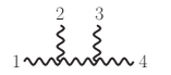
Figure 31: The four-point cubic diagram whose numerator (B.7) determines all other diagram numerators.

We will also need $D$-dimensional versions of tree amplitude in our explicit checks that the four-dimensional trees are sufficient to capture the full classical conservative potential. We express the $D$-dimensional amplitudes in terms of diagrams with only cubic vertices. Using BCJ duality, a simple way to specify all the numerators is in terms of the so-called DDM basis DelDuca:1999rs , where only a single numerator is sufficient to generate the full amplitude. For example, Eq. (5.10) yields the two scalar two gluon amplitude. The BCJ numerator for the four-gluon amplitude corresponding to the diagram in Fig. 31 is

$$n_{s} =n(1,2,3,4)$$

$$=\frac{i}{2}\,\Big{\{}(\varepsilon_{1}\cdot\varepsilon_{4})\left(2(p_{1}\cdot\varepsilon_{2})(p_{12}\cdot\varepsilon_{3})+2(p_{34}\cdot\varepsilon_{2})(p_{4}\cdot\varepsilon_{3})-s(\varepsilon_{2}\cdot\varepsilon_{3})\right)$$

$$\quad+(4(\varepsilon_{3}\cdot\varepsilon_{4})(p_{2}\cdot\varepsilon_{1})(p_{3}\cdot\varepsilon_{2})-4(\varepsilon_{3}\cdot\varepsilon_{4})(p_{3}\cdot\varepsilon_{1})(p_{12}\cdot\varepsilon_{2})-4(\varepsilon_{2}\cdot\varepsilon_{4})(p_{2}\cdot\varepsilon_{1})(p_{12}\cdot\varepsilon_{3}))$$

$$\quad+(4(\varepsilon_{2}\cdot\varepsilon_{1})(p_{3}\cdot\varepsilon_{4})(p_{2}\cdot\varepsilon_{3})-4(\varepsilon_{2}\cdot\varepsilon_{1})(p_{2}\cdot\varepsilon_{4})(p_{34}\cdot\varepsilon_{3})-4(\varepsilon_{3}\cdot\varepsilon_{1})(p_{3}\cdot\varepsilon_{4})(p_{34}\cdot\varepsilon_{2}))$$

$$\quad+2s\,(\varepsilon_{1}\cdot\varepsilon_{3})(\varepsilon_{2}\cdot\varepsilon_{4})+2u\,(\varepsilon_{1}\cdot\varepsilon_{2})(\varepsilon_{3}\cdot\varepsilon_{4})-4(\varepsilon_{2}\cdot\varepsilon_{3})(p_{2}\cdot\varepsilon_{1})(p_{3}\cdot\varepsilon_{4})\Big{\}}\,.$$ (B.7)

Note that under dimensional reduction in Eq. (3.6) and Eq. (3.7), this numerator reduces to $s$-channel numerator in Eq. (5.10). The $u$-channel numerator is given by swapping $2\leftrightarrow 3$,

$$n_{u}=n(1,3,2,4)\,,$$ (B.8)

and the $t$-channel is given by Jacobi identity (3.11)

$$n_{t}=n(1,2,3,4)-n(1,3,2,4)\,.$$ (B.9)

In terms of these numerators, the four-point tree-level gauge-theory amplitude is

$${\cal A}^{\rm tree}_{4}(1,2,3,4)=\frac{n_{s}c_{s}}{s}+\frac{n_{t}c_{t}}{t}+\frac{n_{u}c_{u}}{u}\,,$$ (B.10)

while the gravity amplitude is

$$M^{\rm tree}_{4}(1,2,3,4)=i\Bigl{(}\frac{n_{s}^{2}}{s}+\frac{n_{t}^{2}}{t}+\frac{n_{u}^{2}}{u}\Bigr{)}\,.$$ (B.11)

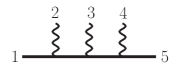
Figure 32: The five-point diagram whose kinematic numerator determines all other diagram numerators.

We also need the $D$-dimensional two-scalar three-gluon tree amplitude. Using again the DDM basis and BCJ duality, we need only specify the numerator corresponding to the diagram in Fig. 32,

$$n(1^{s},2,3,4,5^{s})=\frac{i}{\sqrt{8}}\,\Big{\{} -4(p_{1}\cdot\varepsilon_{2})(p_{12}\cdot\varepsilon_{3})(p_{123}\cdot\varepsilon_{4})-2(\varepsilon_{2}\cdot\varepsilon_{3})(p_{12}\cdot p_{3})\left((p_{1}-p_{5}+2p_{2})\cdot\varepsilon_{4}\right)$$

$$+4(p_{345}\cdot\varepsilon_{2})(p_{45}\cdot\varepsilon_{3})(p_{5}\cdot\varepsilon_{4})+2(\varepsilon_{3}\cdot\varepsilon_{4})(p_{12}\cdot p_{3})\left((p_{1}-p_{5}-2p_{4})\cdot\varepsilon_{2}\right)$$

$$+4(\varepsilon_{2}\cdot\varepsilon_{4})\left((p_{2}\cdot\varepsilon_{3})(p_{4}\cdot p_{5})-(p_{4}\cdot\varepsilon_{3})(p_{1}\cdot p_{2})\right)$$

$$+(\varepsilon_{2}\cdot\varepsilon_{4})((p_{1}-p_{5})\cdot\varepsilon_{3})(p^{2}_{12}+p^{2}_{45}-2m^{2})\Big{\}},$$ (B.12)

where $p_{ijk}=p_{i}+p_{j}+p_{k}$. The propagators and color factors can be read from the diagrams. The diagrams where the scalars are held fixed and the gluon legs are permuted are obtained simply by relabeling the gluon legs $2,3,4$ in Eq. (B.12). The remaining 9 diagram, for a total of 15, are obtained by using the BCJ identities for the kinematic numerator factors $n$. As usual, the full amplitudes are assembled using Eqs.(3.8) or (3.13).

The $D$-dimensional tree-level amplitudes with two scalar lines presented here have the useful property that the on-shell Ward identities,

$$\mathcal{A}|_{\varepsilon_{i}\rightarrow p_{i}}\rightarrow 0\,,$$ (B.13)

hold for the gluon or graviton $i=2,3,\dotsc n-1$ without using transverse property on other legs. Whenever the Ward identity holds without using the transverse properties on any other legs, we will call this a “generalized Ward identity”. An amplitude with this property is obtained by appropriately adding terms that vanish due to on-shell conditions to a generic form that amplitude. The existence of such amplitudes has been exploited in the calculations of Refs. 3PMPRL ; Paolo2PM to help simplify $D$-dimensional constructions of the integrand. We use this property in the calculations in Secs. 5 and 6 to simplify physical-state projectors that appear in $D$-dimensional unitarity cuts.

Appendix C Series Resummation

We collect here the series encountered in Eq. (9.1) and their resummation. We have the simple geometric series and its square:

$$1+\frac{\bm{p}^{2}}{E_{2}^{2}}+\frac{\bm{p}^{4}}{E_{2}^{4}}+\frac{\bm{p}^{6}}{E_{2}^{6}}+\cdots\equiv{E_{2}^{2}\over m_{2}^{2}}\,,$$ (C.1)

$$1+\frac{2\bm{p}^{2}}{E_{2}^{2}}+\frac{3\bm{p}^{4}}{E_{2}^{4}}+\frac{4\bm{p}^{6}}{E_{2}^{6}}+\cdots\equiv{E_{2}^{4}\over m_{2}^{4}}\,,$$

$$1-\frac{\bm{p}^{2}}{3E_{2}^{2}}-\frac{5\bm{p}^{4}}{3E_{2}^{4}}-\frac{3\bm{p}^{6}}{E_{2}^{6}}+\cdots\equiv{7E_{2}^{2}\over 3m_{2}^{2}}-{4E_{2}^{4}\over 3m_{2}^{4}}\,,$$

where the third series is a linear combination of the first two. For the resummation of the IR pieces we encountered the series

$$1+\frac{\bm{p}^{2}}{2E_{2}^{2}}+\frac{3\bm{p}^{4}}{8E_{2}^{4}}+\frac{5\bm{p}^{6}}{16E_{2}^{6}}+\cdots\equiv{E_{2}\over m_{2}}\,,$$ (C.2)

$$1+\frac{3\bm{p}^{2}}{2E_{2}^{2}}+\frac{15\bm{p}^{4}}{8E_{2}^{4}}+\frac{35\bm{p}^{6}}{16E_{2}^{6}}+\cdots\equiv{E_{2}^{3}\over m_{2}^{3}}\,,$$

where the first one is the square root of the geometric series above and is also encountered in the box-triangle example in Sec. 7.3.4.

We have series that involve the expansion of square roots and hence binomial coefficients, which we denote here as ${\rm B}[m,n]$:

$$1+{5\bm{p}^{2}\over 4E_{2}^{2}}+{11\bm{p}^{4}\over 8E_{2}^{4}}+{93\bm{p}^{6}\over 64E_{2}^{6}}+\cdots\equiv 2\sum_{n=0}^{\infty}\left(1+(-1)^{n}{\rm B}[-1/2,n+1]\right){\bm{p}^{2n}\over E_{2}^{2n}}={2E_{2}^{3}(E_{2}-m_{2})\over m_{2}^{2}\bm{p}^{2}}\,,$$ (C.3)

$$1+{7\bm{p}^{2}\over 2E_{2}^{2}}+{51\bm{p}^{4}\over 8E_{2}^{4}}+{151\bm{p}^{6}\over 16E_{2}^{6}}+\cdots\equiv\sum_{n=0}^{\infty}\left(4(n+1)-3(-1)^{n}{\rm B}[-3/2,n]\right){\bm{p}^{2n}\over E_{2}^{2n}}={E_{2}^{3}(4E_{2}-3m_{2})\over m_{2}^{4}}\,.$$

The first series above appears in the example of the two-loop scalar box-triangle integral.

Finally we have series that resum to ${\rm arcsinh}{|\bm{p}|\over m_{i}}$, which is the rapidity of particle $i=1$ or 2:

$$1+{\left(E_{1}^{3}+E_{2}^{3}\right)\over 3E_{1}^{2}E_{2}^{2}E}{\bm{p}}^{2}+\frac{\left(E_{1}^{5}+E_{2}^{5}\right)}{5E_{1}^{4}E_{2}^{4}E}{\bm{p}}^{4}+\frac{\left(E_{1}^{7}+E_{2}^{7}\right)}{7E_{1}^{6}E_{2}^{6}E}{\bm{p}}^{6}+\cdots\equiv{1\over E}\sum_{n=0}^{\infty}{(E_{1}^{2n+1}+E_{2}^{2n+1})\bm{p}^{2n}\over(2n+1)E_{1}^{2n}E_{2}^{2n}}$$ (C.4)

$$\hskip 277.41437pt={E_{1}E_{2}\left[{\rm arcsinh}{|\bm{p}|\over m_{1}}+{\rm arcsinh}{|\bm{p}|\over m_{2}}\right]\over E|\bm{p}|}\,,$$

$$1+{\left(E_{1}^{3}+E_{2}^{3}\right)\over 5E_{1}^{2}E_{2}^{2}E}{\bm{p}}^{2}+\frac{3\left(E_{1}^{5}+E_{2}^{5}\right)}{35E_{1}^{4}E_{2}^{4}E}{\bm{p}}^{4}+\cdots\equiv{3\over E}\sum_{n=0}^{\infty}{(E_{1}^{2n+1}+E_{2}^{2n+1})\bm{p}^{2n}\over(2n+1)(2n+3)E_{1}^{2n}E_{2}^{2n}}$$

$$\hskip 203.43703pt={3E_{1}E_{2}\over 2\bm{p}^{2}}\left[1+{m_{1}^{2}\,{\rm arcsinh}{|\bm{p}|\over m_{1}}+m_{2}^{2}\,{\rm arcsinh}{|\bm{p}|\over m_{2}}\over E|\bm{p}|}\right]\,,$$

$$1+\frac{3\bm{p}^{2}}{5E_{1}^{2}}+\frac{3\bm{p}^{4}}{7E_{1}^{4}}+\cdots\equiv 3\sum_{n=0}^{\infty}{\bm{p}^{2n}\over(2n+3)E_{1}^{2n}}=-{3E_{1}^{2}\over\bm{p}^{2}}+{3E_{1}^{3}{\rm arcsinh}{|\bm{p}|\over m_{1}}\over|\bm{p}|^{3}}\,,$$

$$1+\frac{6\bm{p}^{2}}{5E_{1}^{2}}+\frac{9\bm{p}^{4}}{7E_{1}^{4}}+\cdots\equiv 3\sum_{n=0}^{\infty}{(n+1)\bm{p}^{2n}\over(2n+3)E_{1}^{2n}}={3E_{1}^{4}\over 2m_{1}^{2}\bm{p}^{2}}-{3E_{1}^{3}{\rm arcsinh}{|\bm{p}|\over m_{1}}\over 2|\bm{p}|^{3}}\,.$$

The first series above appears in the example of the two loop scalar flipped double triangle and scalar H integrals.

Note that a few of the series shown in this appendix are related to each other by the operator ${d\over dx}x(\cdot)$, where $x$ is the small parameter. Moreover, notice that the resummation often yields factors of $E_{i}$ that cancel with those multiplying the series in Eq. (9.1). In particular, combining those factors into the series and then expanding in large $m_{i}$ can lead to even simpler series.

Appendix D Evaluation of H Diagram and Imaginary Part

We extract the small-$t$ limit of the H and ${\overline{\rm H}}$ integral which has been calculated for the fully quantum case in Ref. Bianchi:2016yiq for the case of equal masses (motivated by massive-quark scattering). We start from results in the Euclidean region in the aforementioned reference, written in terms of harmonic polylogarithms, and with different notations for the kinematic variables and perform the necessary analytic continuation. The material here differs from Sec. 8.1 in two respects: (1) here we do not give results for tensor integrals; (2) here we present the full $\ln(-t)$ terms of the H integral and ${\overline{\rm H}}$ integral separately, without adding them together to localize on matter poles, and without dropping imaginary contributions. This gives us an important confirmation on our techniques, because the classical limit is taken only at the end, after all loop integrations are carried out in a fully relativistic fashion.

The $\ln(-t)$ term of the scalar H integral in the small-$t$ limit, starting from Eq. (4.1) of Ref. Bianchi:2016yiq , is

$$I_{\rm H}\big{|}_{\ln(-t)}=-\frac{1}{192\pi^{4}}\frac{1}{m^{2}t^{2}}\frac{1}{\sqrt{\sigma^{2}-1}}\operatorname{arcsinh}\sqrt{\frac{\sigma-1}{2}}\left[4\operatorname{arcsinh}^{2}\sqrt{\frac{\sigma-1}{2}}-6i\pi\operatorname{arcsinh}\sqrt{\frac{\sigma-1}{2}}-2\pi^{2}\right],$$ (D.1)

where we have divided by $(-256\pi^{4})$ to account for the difference in normalization compared to the one used here and $\sigma$ is defined in Eq. (7.59), taking $m_{1}=m_{2}=m$. The result for the scalar ${\overline{\rm H}}$ integral is

$$I_{\overline{\rm H}}\big{|}_{\ln(-t)}=\frac{1}{192\pi^{4}}\frac{1}{m^{2}t^{2}}\frac{1}{\sqrt{\sigma^{2}-1}}\operatorname{arcsinh}\sqrt{\frac{\sigma-1}{2}}\left[4\operatorname{arcsinh}^{2}\sqrt{\frac{\sigma-1}{2}}+\pi^{2}\right].$$ (D.2)

Adding Eq. (D.1) and Eq. (D.2) for the H and ${\overline{\rm H}}$ diagram, the $\ln(-t)$ coefficient in the sum is

$$\left(I_{\rm H}+I_{\overline{\rm H}}\right)\big{|}_{\ln(-t)}=\frac{1}{64\pi^{3}}\frac{1}{m^{2}t^{2}}\frac{1}{\sqrt{\sigma^{2}-1}}\operatorname{arcsinh}\sqrt{\frac{\sigma-1}{2}}\left[\pi+2i\operatorname{arcsinh}\sqrt{\frac{\sigma-1}{2}}\right].$$ (D.3)

The real part is in perfect agreement with our previous results in Eqs. (7.78) and (8.10) from expansions around the potential region, after setting $m_{1}=m_{2}=m$ (and accounting for the $1/t^{2}$ extracted from the earlier expressions). Eq. (D.3) also has a nonzero imaginary part as expected, corresponding to the possibility that the internal graviton propagator not attached to the matter lines goes on shell. This term, however, does not contribute to the conservative classical potential. The agreement of the real part of the $\ln(-t)$ coefficient with our result is a direct confirmation of the appearance of a mass singularity in the classical part of this integral, starting with a full quantum evaluation.

References

- (1) B. P. Abbott et al. [LIGO Scientific and Virgo Collaborations], Phys. Rev. Lett. 116, no. 6, 061102 (2016) doi:10.1103/PhysRevLett.116.061102 [arXiv:1602.03837 [gr-qc]].
- (2) B. P. Abbott et al. [LIGO Scientific and Virgo Collaborations], Phys. Rev. Lett. 119, no. 16, 161101 (2017) doi:10.1103/PhysRevLett.119.161101 [arXiv:1710.05832 [gr-qc]].
- (3) A. Buonanno and T. Damour, Phys. Rev. D 59, 084006 (1999) doi:10.1103/PhysRevD.59.084006 [gr-qc/9811091].
- (4) A. Buonanno and T. Damour, Phys. Rev. D 62, 064015 (2000) doi:10.1103/PhysRevD.62.064015 [gr-qc/0001013].
- (5) F. Pretorius, Phys. Rev. Lett. 95, 121101 (2005) doi:10.1103/PhysRevLett.95.121101 [gr-qc/0507014].
- (6) M. Campanelli, C. O. Lousto, P. Marronetti and Y. Zlochower, Phys. Rev. Lett. 96, 111101 (2006) doi:10.1103/PhysRevLett.96.111101 [gr-qc/0511048].
- (7) J. G. Baker, J. Centrella, D. I. Choi, M. Koppitz and J. van Meter, Phys. Rev. Lett. 96, 111102 (2006) doi:10.1103/PhysRevLett.96.111102 [gr-qc/0511103].
- (8) Y. Mino, M. Sasaki and T. Tanaka, Phys. Rev. D 55, 3457 (1997) doi:10.1103/PhysRevD.55.3457 [gr-qc/9606018].
- (9) T. C. Quinn and R. M. Wald, Phys. Rev. D 56, 3381 (1997) doi:10.1103/PhysRevD.56.3381 [gr-qc/9610053].
- (10) J. Droste. “The field of moving centres in Einstein’s theory of gravitation,” Proc. Acad. Sci. Amst. 19:447–455 (1916).
- (11) A. Einstein, L. Infeld and B. Hoffmann, “The Gravitational equations and the problem of motion,” Annals Math. 39, 65 (1938) doi:10.2307/1968714.
- (12) B. Bertotti, “On gravitational motion”, Nuovo Cimento 4:898-906 (1956) doi:10.1007/BF02746175.
- (13) R. P. Kerr, “The Lorentz-covariant approximation method in general relativity”, I. Nuovo Cimento 13:469-491 (1959) doi:10.1007/BF02732767.
- (14) B. Bertotti, J. F. Plebański, “Theory of gravitational perturbations in the fast motion approximation”, Ann, Phys, 11:169-200 (1960) doi:10.1016/0003-4916(60)90132-9.
- (15) M. Portilla, “Momentum and angular momentum of two gravitating particles,” J. Phys. A 12, 1075 (1979) doi:10.1088/0305-4470/12/7/025.
- (16) K. Westpfahl and M. Goller, “Gravitational scattering of two relativistic particles in postlinear approximation,” Lett. Nuovo Cim. 26, 573 (1979) doi:10.1007/BF02817047.
- (17) M. Portilla, “Scattering of two gravitating particles: classical approach,” J. Phys. A 13, 3677 (1980) doi:10.1088/0305-4470/13/12/017.
- (18) L. Bel, T. Damour, N. Deruelle, J. Ibanez and J. Martin, “Poincaré-invariant gravitational field and equations of motion of two pointlike objects: The postlinear approximation of general relativity,” Gen. Rel. Grav. 13, 963 (1981) doi:10.1007/BF00756073.
- (19) T. Ledvinka, G. Schaefer and J. Bicak, “Relativistic closed-form Hamiltonian for many-body gravitating systems in the post-Minkowskian approximation,” Phys. Rev. Lett. 100, 251101 (2008) doi:10.1103/PhysRevLett.100.251101 [arXiv:0807.0214 [gr-qc]].
- (20) K. Westpfahl, “High-speed scattering of charged and uncharged particles in general relativity”, Fortschr. Phys., 33, 417 (1985).
- (21) T. Damour, Phys. Rev. D 94, no. 10, 104015 (2016) doi:10.1103/PhysRevD.94.104015 [arXiv:1609.00354 [gr-qc]].
- (22) T. Damour, “High-energy gravitational scattering and the general relativistic two-body problem,” Phys. Rev. D 97, no. 4, 044038 (2018) doi:10.1103/PhysRevD.97.044038 [arXiv:1710.10599 [gr-qc]].
- (23) W. D. Goldberger and I. Z. Rothstein, “An effective field theory of gravity for extended objects,” Phys. Rev. D 73, 104029 (2006) doi:10.1103/PhysRevD.73.104029 [hep-th/0409156].
- (24) L. Blanchet, Living Rev. Rel. 17, 2 (2014) doi:10.12942/lrr-2014-2 [arXiv:1310.1528 [gr-qc]].
- (25) R. A. Porto, Phys. Rept. 633, 1 (2016) doi:10.1016/j.physrep.2016.04.003 [arXiv:1601.04914 [hep-th]].
- (26) G. Schäfer and P. Jaranowski, Living Rev. Rel. 21, no. 1, 7 (2018) doi:10.1007/s41114-018-0016-5 [arXiv:1805.07240 [gr-qc]].
- (27) L. Barack and A. Pound, Rept. Prog. Phys. 82, no. 1, 016904 (2019) doi:10.1088/1361-6633/aae552 [arXiv:1805.10385 [gr-qc]].
- (28) L. Barack et al., Class. Quant. Grav. 36, no. 14, 143001 (2019) doi:10.1088/1361-6382/ab0587 [arXiv:1806.05195 [gr-qc]].
- (29) M. Levi, arXiv:1807.01699 [hep-th].
- (30) T. Ohta, H. Okamura, T. Kimura and K. Hiida, “Physically acceptable solution of einstein’s equation for many-body system,” Prog. Theor. Phys. 50, 492 (1973) doi:10.1143/PTP.50.492.
- (31) P. Jaranowski and G. Schaefer, Phys. Rev. D 57, 7274 (1998) Erratum: [Phys. Rev. D 63, 029902 (2001)] doi:10.1103/PhysRevD.57.7274, 10.1103/PhysRevD.63.029902 [gr-qc/9712075].
- (32) T. Damour, P. Jaranowski and G. Schaefer, Phys. Rev. D 62, 044024 (2000) doi:10.1103/PhysRevD.62.044024 [gr-qc/9912092].
- (33) L. Blanchet and G. Faye, Phys. Lett. A 271, 58 (2000) doi:10.1016/S0375-9601(00)00360-1 [gr-qc/0004009].
- (34) T. Damour, P. Jaranowski and G. Schaefer, Phys. Lett. B 513, 147 (2001) doi:10.1016/S0370-2693(01)00642-6 [gr-qc/0105038].
- (35) T. Damour, P. Jaranowski and G. Schäfer, “Nonlocal-in-time action for the fourth post-Newtonian conservative dynamics of two-body systems,” Phys. Rev. D 89, no. 6, 064058 (2014) doi:10.1103/PhysRevD.89.064058 [arXiv:1401.4548 [gr-qc]].
- (36) P. Jaranowski and G. Schäfer, “Derivation of local-in-time fourth post-Newtonian ADM Hamiltonian for spinless compact binaries,” Phys. Rev. D 92, no. 12, 124043 (2015) doi:10.1103/PhysRevD.92.124043 [arXiv:1508.01016 [gr-qc]].
- (37) L. Bernard, L. Blanchet, A. Bohé, G. Faye and S. Marsat, Phys. Rev. D 93, no. 8, 084037 (2016) doi:10.1103/PhysRevD.93.084037 [arXiv:1512.02876 [gr-qc]].
- (38) T. Marchand, L. Bernard, L. Blanchet and G. Faye, Phys. Rev. D 97, no. 4, 044023 (2018) doi:10.1103/PhysRevD.97.044023 [arXiv:1707.09289 [gr-qc]].
- (39) S. Foffa and R. Sturani, Phys. Rev. D 87, no. 6, 064011 (2013) doi:10.1103/PhysRevD.87.064011 [arXiv:1206.7087 [gr-qc]].
- (40) S. Foffa, P. Mastrolia, R. Sturani and C. Sturm, Phys. Rev. D 95, no. 10, 104009 (2017) doi:10.1103/PhysRevD.95.104009 [arXiv:1612.00482 [gr-qc]].
- (41) S. Foffa and R. Sturani, Phys. Rev. D 100, no. 2, 024047 (2019) doi:10.1103/PhysRevD.100.024047 [arXiv:1903.05113 [gr-qc]].
- (42) R. A. Porto and I. Z. Rothstein, Phys. Rev. D 96, no. 2, 024062 (2017) doi:10.1103/PhysRevD.96.024062 [arXiv:1703.06433 [gr-qc]].
- (43) S. Foffa, R. A. Porto, I. Rothstein and R. Sturani, Phys. Rev. D 100, no. 2, 024048 (2019) doi:10.1103/PhysRevD.100.024048 [arXiv:1903.05118 [gr-qc]].
- (44) S. Foffa, P. Mastrolia, R. Sturani, C. Sturm and W. J. Torres Bobadilla, Phys. Rev. Lett. 122, no. 24, 241605 (2019) doi:10.1103/PhysRevLett.122.241605 [arXiv:1902.10571 [gr-qc]].
- (45) J. Blümlein, A. Maier and P. Marquard, arXiv:1902.11180 [gr-qc].
- (46) J. Feng, M. Baumann, B. Hall, J. Doss, L. Spencer and R. Matzner, Astrophys. J. 859, no. 2, 130 (2018) doi:10.3847/1538-4357/aac209 [arXiv:1805.00813 [gr-qc]].
- (47) L. Blanchet and A. S. Fokas, Phys. Rev. D 98, no. 8, 084005 (2018) doi:10.1103/PhysRevD.98.084005 [arXiv:1806.08347 [gr-qc]].
- (48) F. Cachazo and A. Guevara, “Leading singularities and classical gravitational scattering,” arXiv:1705.10262 [hep-th].
- (49) D. Bini and T. Damour, Phys. Rev. D 96, no. 10, 104038 (2017) doi:10.1103/PhysRevD.96.104038 [arXiv:1709.00590 [gr-qc]].
- (50) J. Vines, Class. Quant. Grav. 35, no. 8, 084002 (2018) doi:10.1088/1361-6382/aaa3a8 [arXiv:1709.06016 [gr-qc]].
- (51) D. Bini and T. Damour, Phys. Rev. D 98, no. 4, 044036 (2018) doi:10.1103/PhysRevD.98.044036 [arXiv:1805.10809 [gr-qc]].
- (52) A. Guevara, A. Ochirov and J. Vines, arXiv:1812.06895 [hep-th].
- (53) J. Vines, J. Steinhoff and A. Buonanno, Phys. Rev. D 99, no. 6, 064054 (2019) doi:10.1103/PhysRevD.99.064054 [arXiv:1812.00956 [gr-qc]].
- (54) M. Z. Chung, Y. T. Huang, J. W. Kim and S. Lee, JHEP 1904, 156 (2019) doi:10.1007/JHEP04(2019)156 [arXiv:1812.08752 [hep-th]].
- (55) B. Maybee, D. O’Connell and J. Vines, arXiv:1906.09260 [hep-th].
- (56) A. Guevara, A. Ochirov and J. Vines, arXiv:1906.10071 [hep-th].
- (57) J. Plefka, J. Steinhoff and W. Wormsbecher, “Effective action of dilaton gravity as the classical double copy of Yang-Mills theory,” Phys. Rev. D 99, no. 2, 024021 (2019) doi:10.1103/PhysRevD.99.024021 [arXiv:1807.09859 [hep-th]].
- (58) C. Cheung, I. Z. Rothstein and M. P. Solon, “From scattering amplitudes to classical potentials in the post-Minkowskian expansion,” Phys. Rev. Lett. 121, no. 25, 251101 (2018) doi:10.1103/PhysRevLett.121.251101 [arXiv:1808.02489 [hep-th]].
- (59) Z. Bern, C. Cheung, R. Roiban, C. H. Shen, M. P. Solon and M. Zeng, “Scattering amplitudes and the conservative Hamiltonian for binary systems at third post-Minkowskian order,” Phys. Rev. Lett. 122, no. 20, 201603 (2019) doi:10.1103/PhysRevLett.122.201603 [arXiv:1901.04424 [hep-th]].
- (60) A. Koemans Collado, P. Di Vecchia and R. Russo, “Revisiting the 2PM eikonal and the dynamics of binary black holes,” arXiv:1904.02667 [hep-th].
- (61) A. Cristofoli, N. E. J. Bjerrum-Bohr, P. H. Damgaard and P. Vanhove, arXiv:1906.01579 [hep-th].
- (62) A. Brandhuber and G. Travaglini, arXiv:1905.05657 [hep-th].
- (63) A. Cristofoli, arXiv:1906.05209 [hep-th].
- (64) Y. Iwasaki, Prog. Theor. Phys. 46, 1587 (1971). doi:10.1143/PTP.46.1587
- (65) Y. Iwasaki, Lett. Nuovo Cim. 1S2, 783 (1971) [Lett. Nuovo Cim. 1, 783 (1971)]. doi:10.1007/BF02770190
- (66) S. N. Gupta and S. F. Radford, Phys. Rev. D 19, 1065 (1979). doi:10.1103/PhysRevD.19.1065
- (67) J. F. Donoghue, Phys. Rev. D 50, 3874 (1994) doi:10.1103/PhysRevD.50.3874 [gr-qc/9405057].
- (68) B. R. Holstein and J. F. Donoghue, Phys. Rev. Lett. 93, 201602 (2004) doi:10.1103/PhysRevLett.93.201602 [hep-th/0405239].
- (69) D. Neill and I. Z. Rothstein, “Classical space-times from the S matrix,” Nucl. Phys. B 877, 177 (2013) doi:10.1016/j.nuclphysb.2013.09.007 [arXiv:1304.7263 [hep-th]].
- (70) V. Vaidya, Phys. Rev. D 91, no. 2, 024017 (2015) doi:10.1103/PhysRevD.91.024017 [arXiv:1410.5348 [hep-th]].
- (71) D. A. Kosower, B. Maybee and D. O’Connell, “Amplitudes, observables, and classical scattering,” JHEP 1902, 137 (2019) doi:10.1007/JHEP02(2019)137 [arXiv:1811.10950 [hep-th]].
- (72) A. Antonelli, A. Buonanno, J. Steinhoff, M. van de Meent and J. Vines, Phys. Rev. D 99, no. 10, 104004 (2019) doi:10.1103/PhysRevD.99.104004 [arXiv:1901.07102 [gr-qc]].
- (73) Z. Bern, L. J. Dixon, D. C. Dunbar and D. A. Kosower, Nucl. Phys. B 425, 217 (1994) doi:10.1016/0550-3213(94)90179-1 [hep-ph/9403226].
- (74) Z. Bern, L. J. Dixon, D. C. Dunbar and D. A. Kosower, Nucl. Phys. B 435, 59 (1995) doi:10.1016/0550-3213(94)00488-Z [hep-ph/9409265].
- (75) Z. Bern, L. J. Dixon and D. A. Kosower, Nucl. Phys. B 513, 3 (1998) doi:10.1016/S0550-3213(97)00703-7 [hep-ph/9708239].
- (76) R. Britto, F. Cachazo and B. Feng, Nucl. Phys. B 725, 275 (2005) doi:10.1016/j.nuclphysb.2005.07.014 [hep-th/0412103].
- (77) Z. Bern, J. J. M. Carrasco, H. Johansson and D. A. Kosower, Phys. Rev. D 76, 125020 (2007) doi:10.1103/PhysRevD.76.125020 [arXiv:0705.1864 [hep-th]].
- (78) Z. Bern, L. J. Dixon and D. A. Kosower, Ann. Rev. Nucl. Part. Sci. 46, 109 (1996) doi:10.1146/annurev.nucl.46.1.109 [hep-ph/9602280].
- (79) Z. Bern and Y. t. Huang, J. Phys. A 44, 454003 (2011) doi:10.1088/1751-8113/44/45/454003 [arXiv:1103.1869 [hep-th]].
- (80) J. J. M. Carrasco and H. Johansson, J. Phys. A 44, 454004 (2011) doi:10.1088/1751-8113/44/45/454004 [arXiv:1103.3298 [hep-th]].
- (81) H. Kawai, D. C. Lewellen and S. H. H. Tye, “A relation between tree amplitudes of closed and open strings,” Nucl. Phys. B 269, 1 (1986). doi:10.1016/0550-3213(86)90362-7
- (82) Z. Bern, J. J. M. Carrasco and H. Johansson, “New relations for gauge-theory amplitudes,” Phys. Rev. D 78, 085011 (2008) doi:10.1103/PhysRevD.78.085011 [arXiv:0805.3993 [hep-ph]].
- (83) Z. Bern, J. J. M. Carrasco and H. Johansson, “Perturbative quantum gravity as a double copy of gauge theory,” Phys. Rev. Lett. 105, 061602 (2010) doi:10.1103/PhysRevLett.105.061602 [arXiv:1004.0476 [hep-th]].
- (84) Z. Bern, J. J. M. Carrasco, L. J. Dixon, H. Johansson and R. Roiban, “Simplifying multiloop integrands and ultraviolet divergences of gauge theory and gravity amplitudes,” Phys. Rev. D 85, 105014 (2012) doi:10.1103/PhysRevD.85.105014 [arXiv:1201.5366 [hep-th]];
- (85) Z. Bern, J. J. Carrasco, L. J. Dixon, H. Johansson and R. Roiban, Phys. Rev. Lett. 103, 081301 (2009) doi:10.1103/PhysRevLett.103.081301 [arXiv:0905.2326 [hep-th]].
- (86) Z. Bern, S. Davies, T. Dennen, A. V. Smirnov and V. A. Smirnov, Phys. Rev. Lett. 111, no. 23, 231302 (2013) doi:10.1103/PhysRevLett.111.231302 [arXiv:1309.2498 [hep-th]].
- (87) Z. Bern, S. Davies and T. Dennen, Phys. Rev. D 90, no. 10, 105011 (2014) doi:10.1103/PhysRevD.90.105011 [arXiv:1409.3089 [hep-th]].
- (88) Z. Bern, J. J. M. Carrasco, W. M. Chen, H. Johansson, R. Roiban and M. Zeng, Phys. Rev. D 96, no. 12, 126012 (2017) doi:10.1103/PhysRevD.96.126012 [arXiv:1708.06807 [hep-th]].
- (89) Z. Bern, J. J. Carrasco, W. M. Chen, A. Edison, H. Johansson, J. Parra-Martinez, R. Roiban and M. Zeng, Phys. Rev. D 98, no. 8, 086021 (2018) doi:10.1103/PhysRevD.98.086021 [arXiv:1804.09311 [hep-th]].
- (90) Z. Bern, C. Cheung, H. H. Chi, S. Davies, L. Dixon and J. Nohle, Phys. Rev. Lett. 115, no. 21, 211301 (2015) doi:10.1103/PhysRevLett.115.211301 [arXiv:1507.06118 [hep-th]].
- (91) Z. Bern, H. H. Chi, L. Dixon and A. Edison, Phys. Rev. D 95, no. 4, 046013 (2017) doi:10.1103/PhysRevD.95.046013 [arXiv:1701.02422 [hep-th]].
- (92) F. A. Berends, R. Kleiss, P. De Causmaecker, R. Gastmans and T. T. Wu, Phys. Lett. 103B, 124 (1981). doi:10.1016/0370-2693(81)90685-7
- (93) F. A. Berends, R. Kleiss, P. De Causmaecker, R. Gastmans, W. Troost and T. T. Wu, Nucl. Phys. B 206, 61 (1982). doi:10.1016/0550-3213(82)90489-8
- (94) Z. Xu, D. H. Zhang and L. Chang, Nucl. Phys. B 291, 392 (1987). doi:10.1016/0550-3213(87)90479-2
- (95) M. Beneke and V. A. Smirnov, Nucl. Phys. B 522, 321 (1998) doi:10.1016/S0550-3213(98)00138-2 [hep-ph/9711391].
- (96) V. A. Smirnov, Springer Tracts Mod. Phys. 211, 1 (2004).
- (97) M. S. Bianchi and M. Leoni, Phys. Lett. B 777, 394 (2018) doi:10.1016/j.physletb.2017.12.030 [arXiv:1612.05609 [hep-ph]].
- (98) T. Damour and G. Esposito-Farese, Phys. Rev. D 58, 042001 (1998) doi:10.1103/PhysRevD.58.042001 [gr-qc/9803031].
- (99) T. Hinderer, Astrophys. J. 677, 1216 (2008) doi:10.1086/533487 [arXiv:0711.2420 [astro-ph]].
- (100) T. Damour and A. Nagar, Phys. Rev. D 80, 084035 (2009) doi:10.1103/PhysRevD.80.084035 [arXiv:0906.0096 [gr-qc]].
- (101) T. Binnington and E. Poisson, Phys. Rev. D 80, 084018 (2009) doi:10.1103/PhysRevD.80.084018 [arXiv:0906.1366 [gr-qc]].
- (102) B. Kol and M. Smolkin, JHEP 1202, 010 (2012) doi:10.1007/JHEP02(2012)010 [arXiv:1110.3764 [hep-th]].
- (103) N. Gürlebeck, Phys. Rev. Lett. 114, no. 15, 151102 (2015) doi:10.1103/PhysRevLett.114.151102 [arXiv:1503.03240 [gr-qc]].
- (104) R. A. Porto, Fortsch. Phys. 64, no. 10, 723 (2016) doi:10.1002/prop.201600064 [arXiv:1606.08895 [gr-qc]].
- (105) D. N. Kabat and M. Ortiz, “Eikonal quantum gravity and Planckian scattering,” Nucl. Phys. B 388, 570 (1992) doi:10.1016/0550-3213(92)90627-N [hep-th/9203082].
- (106) A. Le Tiec, E. Barausse and A. Buonanno, Phys. Rev. Lett. 108, 131103 (2012) doi:10.1103/PhysRevLett.108.131103 [arXiv:1111.5609 [gr-qc]].
- (107) R. Akhoury, R. Saotome and G. Sterman, “High energy scattering in perturbative quantum gravity at next to leading power,” arXiv:1308.5204 [hep-th].
- (108) N. E. J. Bjerrum-Bohr, P. H. Damgaard, G. Festuccia, L. Planté and P. Vanhove, “General relativity from scattering amplitudes,” Phys. Rev. Lett. 121, no. 17, 171601 (2018) doi:10.1103/PhysRevLett.121.171601 [arXiv:1806.04920 [hep-th]].
- (109) Z. Bern, J. S. Rozowsky and B. Yan, “Two loop four gluon amplitudes in N=4 superYang-Mills,” Phys. Lett. B 401, 273 (1997) doi:10.1016/S0370-2693(97)00413-9 [hep-ph/9702424].
- (110) Z. Bern, L. J. Dixon, D. C. Dunbar, M. Perelstein and J. S. Rozowsky, “On the relationship between Yang-Mills theory and gravity and its implication for ultraviolet divergences,” Nucl. Phys. B 530, 401 (1998) doi:10.1016/S0550-3213(98)00420-9 [hep-th/9802162].
- (111) Z. Bern, L. J. Dixon, M. Perelstein and J. S. Rozowsky, “Multileg one loop gravity amplitudes from gauge theory,” Nucl. Phys. B 546, 423 (1999) doi:10.1016/S0550-3213(99)00029-2 [hep-th/9811140].
- (112) M. E. Peskin and D. V. Schroeder, “An Introduction to quantum field theory,” Reading, USA: Addison-Wesley (1995)
- (113) N. E. J. Bjerrum-Bohr, P. H. Damgaard, T. Sondergaard and P. Vanhove, JHEP 1101, 001 (2011) doi:10.1007/JHEP01(2011)001 [arXiv:1010.3933 [hep-th]].
- (114) C. R. Mafra, O. Schlotterer and S. Stieberger, JHEP 1107, 092 (2011) doi:10.1007/JHEP07(2011)092 [arXiv:1104.5224 [hep-th]].
- (115) N. E. J. Bjerrum-Bohr, J. L. Bourjaily, P. H. Damgaard and B. Feng, JHEP 1609, 094 (2016) doi:10.1007/JHEP09(2016)094 [arXiv:1608.00006 [hep-th]].
- (116) C. H. Fu, Y. J. Du, R. Huang and B. Feng, JHEP 1709, 021 (2017) doi:10.1007/JHEP09(2017)021 [arXiv:1702.08158 [hep-th]].
- (117) F. Teng and B. Feng, JHEP 1705, 075 (2017) doi:10.1007/JHEP05(2017)075 [arXiv:1703.01269 [hep-th]].
- (118) H. Johansson and A. Ochirov, JHEP 1511, 046 (2015) doi:10.1007/JHEP11(2015)046 [arXiv:1407.4772 [hep-th]].
- (119) H. Johansson and A. Ochirov, JHEP 1601, 170 (2016) doi:10.1007/JHEP01(2016)170 [arXiv:1507.00332 [hep-ph]].
- (120) H. Johansson and A. Ochirov, JHEP 1909, 040 (2019) doi:10.1007/JHEP09(2019)040 [arXiv:1906.12292 [hep-th]].
- (121) M. L. Mangano and S. J. Parke, Phys. Rept. 200, 301 (1991) doi:10.1016/0370-1573(91)90091-Y [hep-th/0509223].
- (122) L. J. Dixon, hep-ph/9601359.
- (123) Z. Bern and A. G. Morgan, “Massive loop amplitudes from unitarity,” Nucl. Phys. B 467, 479 (1996) doi:10.1016/0550-3213(96)00078-8 [hep-ph/9511336].
- (124) N. E. J. Bjerrum-Bohr, J. F. Donoghue and P. Vanhove, “On-shell techniques and universal results in quantum gravity,” JHEP 1402, 111 (2014) doi:10.1007/JHEP02(2014)111 [arXiv:1309.0804 [hep-th]].
- (125) J. C. Collins, “Renormalization : An introduction to renormalization, the renormalization group, and the operator product expansion,” Cambridge University Press (1984) doi:10.1017/CBO9780511622656
- (126) Z. Bern and D. A. Kosower, Nucl. Phys. B 379, 451 (1992). doi:10.1016/0550-3213(92)90134-W
- (127) Z. Bern, A. De Freitas, L. J. Dixon and H. L. Wong, Phys. Rev. D 66, 085002 (2002) doi:10.1103/PhysRevD.66.085002 [hep-ph/0202271].
- (128) Z. Bern, L. J. Dixon and D. A. Kosower, “Two-loop splitting amplitudes in QCD,” JHEP 0408, 012 (2004) doi:10.1088/1126-6708/2004/08/012 [hep-ph/0404293].
- (129) Z. Bern, A. De Freitas and L. J. Dixon, JHEP 0203, 018 (2002) doi:10.1088/1126-6708/2002/03/018 [hep-ph/0201161].
- (130) See the ancillary files of this manuscript.
- (131) W. Bonnor, “Spherical gravitational waves,” Philos. Trans. R. Soc. London, Ser. A 251, 233 (1959).
- (132) W. Bonnor and M. Rotenberg, “Gravitational waves from isolated sources,” Proc. R. Soc. London, Ser. A 289, 247 (1966).
- (133) K. S. Thorne, “Multipole expansions of gravitational radiation,” Rev. Mod. Phys. 52, 299 (1980), doi:10.1103/RevModPhys.52.299.
- (134) L. Blanchet and T. Damour, “Tail transported temporal correlations in the dynamics of a gravitating system,” Phys. Rev. D 37, 1410 (1988), doi:10.1103/PhysRevD.37.1410.
- (135) L. Blanchet and T. Damour, “Hereditary effects in gravitational radiation,” Phys. Rev. D 46, 4304 (1992), doi:10.1103/PhysRevD.46.4304.
- (136) C. R. Galley, A. K. Leibovich, R. A. Porto and A. Ross, “Tail effect in gravitational radiation reaction: Time nonlocality and renormalization group evolution,” Phys. Rev. D 93, 124010 (2016) doi:10.1103/PhysRevD.93.124010 [arXiv:1511.07379 [gr-qc]].
- (137) K. G. Chetyrkin and F. V. Tkachov, Nucl. Phys. B 192, 159 (1981). doi:10.1016/0550-3213(81)90199-1
- (138) S. Laporta, Int. J. Mod. Phys. A 15, 5087 (2000) doi:10.1016/S0217-751X(00)00215-7, 10.1142/S0217751X00002157 [hep-ph/0102033].
- (139) A. V. Kotikov, Phys. Lett. B 254, 158 (1991). doi:10.1016/0370-2693(91)90413-K
- (140) Z. Bern, L. J. Dixon and D. A. Kosower, Nucl. Phys. B 412, 751 (1994) doi:10.1016/0550-3213(94)90398-0 [hep-ph/9306240].
- (141) E. Remiddi, Nuovo Cim. A 110, 1435 (1997) [hep-th/9711188].
- (142) T. Gehrmann and E. Remiddi, “Differential equations for two loop four point functions,” Nucl. Phys. B 580, 485 (2000) doi:10.1016/S0550-3213(00)00223-6 [hep-ph/9912329].
- (143) P. Maierhöfer, J. Usovitsch and P. Uwer, Comput. Phys. Commun. 230, 99 (2018) doi:10.1016/j.cpc.2018.04.012 [arXiv:1705.05610 [hep-ph]].
- (144) I. Dubovyk, J. Gluza, T. Riemann and J. Usovitsch, PoS LL 2016, 034 (2016) doi:10.22323/1.260.0034 [arXiv:1607.07538 [hep-ph]].
- (145) A. Freitas and Y. C. Huang, JHEP 1004, 074 (2010) doi:10.1007/JHEP04(2010)074 [arXiv:1001.3243 [hep-ph]].
- (146) J. Gluza, T. Jelinski and D. A. Kosower, Phys. Rev. D 95, no. 7, 076016 (2017) doi:10.1103/PhysRevD.95.076016 [arXiv:1609.09111 [hep-ph]].
- (147) J. Gluza, K. Kajda and T. Riemann, Comput. Phys. Commun. 177, 879 (2007) doi:10.1016/j.cpc.2007.07.001 [arXiv:0704.2423 [hep-ph]].
- (148) V. A. Smirnov, Phys. Lett. B 460, 397 (1999) doi:10.1016/S0370-2693(99)00777-7 [hep-ph/9905323].
- (149) J. B. Tausk, Phys. Lett. B 469, 225 (1999) doi:10.1016/S0370-2693(99)01277-0 [hep-ph/9909506].
- (150) V. A. Smirnov, Phys. Lett. B 567, 193 (2003) doi:10.1016/S0370-2693(03)00895-5 [hep-ph/0305142].
- (151) G. Heinrich and V. A. Smirnov, Phys. Lett. B 598, 55 (2004) doi:10.1016/j.physletb.2004.07.058 [hep-ph/0406053].
- (152) Z. Bern, L. J. Dixon and V. A. Smirnov, Phys. Rev. D 72, 085001 (2005) doi:10.1103/PhysRevD.72.085001 [hep-th/0505205].
- (153) M. Czakon, Comput. Phys. Commun. 175, 559 (2006) doi:10.1016/j.cpc.2006.07.002 [hep-ph/0511200].
- (154) A. V. Smirnov and V. A. Smirnov, Eur. Phys. J. C 62, 445 (2009) doi:10.1140/epjc/s10052-009-1039-6 [arXiv:0901.0386 [hep-ph]].
- (155) M. Ochman and T. Riemann, Acta Phys. Polon. B 46, no. 11, 2117 (2015) doi:10.5506/APhysPolB.46.2117 [arXiv:1511.01323 [hep-ph]].
- (156) A. V. Smirnov and M. N. Tentyukov, Comput. Phys. Commun. 180, 735 (2009) doi:10.1016/j.cpc.2008.11.006 [arXiv:0807.4129 [hep-ph]].
- (157) A. V. Smirnov, Comput. Phys. Commun. 204, 189 (2016) doi:10.1016/j.cpc.2016.03.013 [arXiv:1511.03614 [hep-ph]].
- (158) S. Borowka, J. Carter and G. Heinrich, J. Phys. Conf. Ser. 368, 012051 (2012) doi:10.1088/1742-6596/366/1/012051 [arXiv:1206.4908 [hep-ph]].
- (159) S. Weinberg, Phys. Rev. 140, B516 (1965). doi:10.1103/PhysRev.140.B516
- (160) S. G. Naculich and H. J. Schnitzer, JHEP 1105, 087 (2011) doi:10.1007/JHEP05(2011)087 [arXiv:1101.1524 [hep-th]].
- (161) R. Akhoury, R. Saotome and G. Sterman, Phys. Rev. D 84, 104040 (2011) doi:10.1103/PhysRevD.84.104040 [arXiv:1109.0270 [hep-th]].
- (162) A. V. Manohar and I. W. Stewart, Phys. Rev. D 62, 074015 (2000) doi:10.1103/PhysRevD.62.074015 [hep-ph/0003032].
- (163) T. Damour, P. Jaranowski and G. Schäfer, “Poincare invariance in the ADM Hamiltonian approach to the general relativistic two-body problem,” Phys. Rev. D 62, 021501 (2000) Erratum: [Phys. Rev. D 63, 029903 (2001)] doi:10.1103/PhysRevD.63.029903, 10.1103/PhysRevD.62.021501 [gr-qc/0003051].
- (164) N. E. J. Bjerrum-Bohr, J. F. Donoghue and B. R. Holstein, Phys. Rev. D 67, 084033 (2003) Erratum: [Phys. Rev. D 71, 069903 (2005)] doi:10.1103/PhysRevD.71.069903, 10.1103/PhysRevD.67.084033 [hep-th/0211072].
- (165) B. R. Holstein and A. Ross, arXiv:0802.0716 [hep-ph].
- (166) N. Wex and G. Schäfer, “Innermost stable orbits for coalescing binary systems of compact objects-a remark” Class. Quantum Grav. 10, 2729 (1993). http://stacks.iop.org/0264-9381/10/i=12/a=028
- (167) D. Bini and T. Damour, Phys. Rev. D 96, no. 6, 064021 (2017) doi:10.1103/PhysRevD.96.064021 [arXiv:1706.06877 [gr-qc]].
- (168) D. Amati, M. Ciafaloni and G. Veneziano, “Higher order gravitational deflection and soft bremsstrahlung in Planckian energy superstring collisions,” Nucl. Phys. B 347, 550 (1990), doi:10.1016/0550-3213(90)90375-N.
- (169) Z. Bern and G. Chalmers, Nucl. Phys. B 447, 465 (1995) doi:10.1016/0550-3213(95)00226-I [hep-ph/9503236].
- (170) N. E. J. Bjerrum-Bohr, J. F. Donoghue, B. R. Holstein, L. Planté and P. Vanhove, “Bending of light in quantum gravity,” Phys. Rev. Lett. 114, no. 6, 061301 (2015) doi:10.1103/PhysRevLett.114.061301 [arXiv:1410.7590 [hep-th]].
- (171) Z. Bern, J. J. Carrasco, W. M. Chen, H. Johansson and R. Roiban, “Gravity amplitudes as generalized double copies of gauge-theory amplitudes,” Phys. Rev. Lett. 118, no. 18, 181602 (2017) doi:10.1103/PhysRevLett.118.181602 [arXiv:1701.02519 [hep-th]].
- (172) R. K. Ellis and G. Zanderighi, JHEP 0802, 002 (2008) doi:10.1088/1126-6708/2008/02/002 [arXiv:0712.1851 [hep-ph]].
- (173) W. Beenakker and A. Denner, Nucl. Phys. B 338, 349 (1990). doi:10.1016/0550-3213(90)90636-R
- (174) P. A. Baikov, Phys. Lett. B 385, 404 (1996) doi:10.1016/0370-2693(96)00835-0 [hep-ph/9603267].
- (175) P. A. Baikov, Nucl. Instrum. Meth. A 389, 347 (1997) doi:10.1016/S0168-9002(97)00126-5 [hep-ph/9611449].
- (176) A. G. Grozin, Int. J. Mod. Phys. A 26, 2807 (2011) doi:10.1142/S0217751X11053687 [arXiv:1104.3993 [hep-ph]].
- (177) H. Frellesvig and C. G. Papadopoulos, JHEP 1704, 083 (2017) doi:10.1007/JHEP04(2017)083 [arXiv:1701.07356 [hep-ph]].
- (178) K. J. Larsen and Y. Zhang, Phys. Rev. D 93, no. 4, 041701 (2016) doi:10.1103/PhysRevD.93.041701 [arXiv:1511.01071 [hep-th]].
- (179) W. L. Burke and K. S. Thorne, doi:10.1007/978-1-4684-0721-1-12
- (180) K. S. Thorne, Astrophys. J. 158, 997 (1969). doi:10.1086/150259
- (181) W. L. Burke, J. Math. Phys. 12, 401 (1971). doi:10.1063/1.1665603
- (182) S. Foffa and R. Sturani, arXiv:1907.02869 [gr-qc].
- (183) S. D. Badger, E. W. N. Glover, V. V. Khoze and P. Svrcek, “Recursion relations for gauge theory amplitudes with massive particles,” JHEP 0507, 025 (2005) doi:10.1088/1126-6708/2005/07/025 [hep-th/0504159].
- (184) A. Luna, R. Monteiro, I. Nicholson, D. O’Connell and C. D. White, JHEP 1606, 023 (2016) doi:10.1007/JHEP06(2016)023 [arXiv:1603.05737 [hep-th]].
- (185) W. D. Goldberger and A. K. Ridgway, Phys. Rev. D 95, no. 12, 125010 (2017) doi:10.1103/PhysRevD.95.125010 [arXiv:1611.03493 [hep-th]].
- (186) W. D. Goldberger, S. G. Prabhu and J. O. Thompson, Phys. Rev. D 96, no. 6, 065009 (2017) doi:10.1103/PhysRevD.96.065009 [arXiv:1705.09263 [hep-th]].
- (187) W. D. Goldberger and A. K. Ridgway, Phys. Rev. D 97, no. 8, 085019 (2018) doi:10.1103/PhysRevD.97.085019 [arXiv:1711.09493 [hep-th]].
- (188) D. Chester, Phys. Rev. D 97, no. 8, 084025 (2018) doi:10.1103/PhysRevD.97.084025 [arXiv:1712.08684 [hep-th]].
- (189) W. D. Goldberger, J. Li and S. G. Prabhu, Phys. Rev. D 97, no. 10, 105018 (2018) doi:10.1103/PhysRevD.97.105018 [arXiv:1712.09250 [hep-th]].
- (190) J. Li and S. G. Prabhu, Phys. Rev. D 97, no. 10, 105019 (2018) doi:10.1103/PhysRevD.97.105019 [arXiv:1803.02405 [hep-th]].
- (191) C. H. Shen, JHEP 1811, 162 (2018) doi:10.1007/JHEP11(2018)162 [arXiv:1806.07388 [hep-th]].
- (192) Y. F. Bautista and A. Guevara, arXiv:1903.12419 [hep-th].
- (193) A. Laddha and A. Sen, JHEP 1809, 105 (2018) doi:10.1007/JHEP09(2018)105 [arXiv:1801.07719 [hep-th]].
- (194) A. Laddha and A. Sen, JHEP 1810, 056 (2018) doi:10.1007/JHEP10(2018)056 [arXiv:1804.09193 [hep-th]].
- (195) A. Laddha and A. Sen, Phys. Rev. D 100, no. 2, 024009 (2019) doi:10.1103/PhysRevD.100.024009 [arXiv:1806.01872 [hep-th]].
- (196) B. Sahoo and A. Sen, JHEP 1902, 086 (2019) doi:10.1007/JHEP02(2019)086 [arXiv:1808.03288 [hep-th]].
- (197) M. Ciafaloni, D. Colferai and G. Veneziano, Phys. Rev. D 99, no. 6, 066008 (2019) doi:10.1103/PhysRevD.99.066008 [arXiv:1812.08137 [hep-th]].
- (198) A. Laddha and A. Sen, arXiv:1906.08288 [gr-qc].
- (199) A. PV and A. Manu, arXiv:1907.10021 [hep-th].
- (200) S. J. Parke and T. R. Taylor, Phys. Rev. Lett. 56, 2459 (1986). doi:10.1103/PhysRevLett.56.2459
- (201) M. L. Mangano, S. J. Parke and Z. Xu, Nucl. Phys. B 298, 653 (1988). doi:10.1016/0550-3213(88)90001-6
- (202) V. Del Duca, L. J. Dixon and F. Maltoni, Nucl. Phys. B 571, 51 (2000) doi:10.1016/S0550-3213(99)00809-3 [hep-ph/9910563].