Two-Loop Master Integrals for the mixed EW-QCD virtual corrections to Drell-Yan scattering

Abstract

We present the calculation of the master integrals needed for the two-loop QCD$\times$EW corrections to $q+\bar{q}\to l^{-}+l^{+}$ and $q+\bar{q}^{\prime}\to l^{-}+\overline{\nu}\,,$ for massless external particles. We treat $W$ and $Z$ bosons as degenerate in mass. We identify three types of diagrams, according to the presence of massive internal lines: the no-mass type, the one-mass type, and the two-mass type, where all massive propagators, when occurring, contain the same mass value. We find a basis of 49 master integrals and evaluate them with the method of the differential equations. The Magnus exponential is employed to choose a set of master integrals that obeys a canonical system of differential equations. Boundary conditions are found either by matching the solutions onto simpler integrals in special kinematic configurations, or by requiring the regularity of the solution at pseudo-thresholds. The canonical master integrals are finally given as Taylor series around $d=4$ space-time dimensions, up to order four, with coefficients given in terms of iterated integrals, respectively up to weight four.

1 Introduction

The Drell-Yan production of $Z$ and $W$ bosons Drell:1970wh is one of the standard candles for physical studies at the LHC. Due to the big cross section and clean experimental signature, Drell-Yan processes can be measured with small experimental uncertainty and, therefore, allow for very precise tests of the Standard Model of fundamental interactions (SM). They give access to the determination of important parameters of the weak sector, as for instance the sine of the weak mixing angle and the $W$ boson mass, that together with the top and the Higgs masses provides stringent constraints on the validity of the SM at the TeV energy scale. Furthermore, Drell-Yan processes constitute the SM background in searches of New Physics, involving for instance new vector boson resonances, $Z^{\prime}$ and $W^{\prime}$, originating from GUT extensions of the SM. Finally, the Drell-Yan mechanism is used for constraining parton distribution functions, for detector calibration and determination of the collider luminosity. For all these reasons, an accurate and reliable experimental and theoretical control on Drell-Yan processes would be of the maximum importance for future physics studies at colliders.

The theoretical description of Drell-Yan processes currently includes NNLO QCD and NLO EW radiative corrections, implemented in flexible tools able to provide predictions for inclusive observables as well as kinematic distributions. Current theoretical predictions are in good agreement with the experimental measurements. However, higher theoretical accuracy is needed in order to match the future experimental requirements, in particular in view of the run II of the LHC. A consistent part of an increasing theoretical accuracy regards higher-order perturbative corrections.

Very recently, NNNLO QCD corrections were calculated for the Higgs total production cross section in gluon-gluon fusion Anastasiou:2015ema ; Anastasiou:2016cez . The residual factorization/renormalization scales variation moved from about 10-15% of the NNLO calculation (supplemented by NNLL resummation) to about 5% of the current result. These results will be applied to Drell-Yan as well, since they involve the evaluation of the same topologies for the calculation of the corresponding Feynman diagrams Gehrmann:2006wg ; Heinrich:2007at ; Heinrich:2009be ; Baikov:2009bg ; Lee:2010cga ; Gehrmann:2010ue .

At the same order of accuracy (one can roughly thing to exchange two powers of $\alpha_{S}$ with one power of $\alpha$), the mixed QCD-EW corrections have to be taken into account. As in the case of QCD NNLO with EW NLO perturbative corrections, the mixed QCD-EW corrections are expected to become of similar size with respect to QCD NNNLO at high leptonic invariant mass Andersen:2014efa .

At LO, the partonic process in the SM is mediated by the exchange of a photon or a $Z$/$W$ vector boson, in the $s$ annihilation channel: $q\bar{q}\to\gamma,Z\to l^{-}l^{+}$ and $q\bar{q^{\prime}}\to W\to l\nu$.

At higher orders in the coupling constants, we can distinguish between QCD and electroweak (EW) or mixed (EW-QCD) corrections to the LO process. In the first case, only the initial state receives quantum corrections, since the leptonic final state does not couple to gluons.

The NLO QCD corrections to the total cross section were calculated in Altarelli:1979ub ; Altarelli:1984pt and revealed a sizable increase of the cross section with respect to the LO result. The NNLO QCD corrections Matsuura:1988sm ; Hamberg:1990np stabilized, then, the convergence of the perturbative series.

QCD fixed-order corrections to the total production cross section are supplemented by the resummation of soft-gluon logarithmically enhanced terms, up to NNNLL approximation Sterman:1986aj ; Catani:1989ne ; Catani:1990rp ; Moch:2005ky .

EW quantum corrections allow exchanges of quanta between initial and final states. Therefore, already at the NLO, massive four-point functions have to be evaluated. Since the bulk of the corrections for inclusive observables comes from the resonant region, in which the exchanged vector boson is nearly on-shell, electroweak NLO corrections to the total cross section were calculated for the $W$ Wackeroth:1996hz and $Z$ Baur:1997wa in narrow-width approximation.

More exclusive observables are known in the literature. The $Z$ and $W$ production at non-zero transverse momentum $p_{T}$ is known at the NLO in QCD Ellis:1981hk ; Arnold:1988dp ; Gonsalves:1989ar ; Brandt:1990vn ; Giele:1993dj ; Dixon:1998py and in the full SM Kuhn:2004em . The two-loop QCD helicity amplitudes for the production of a $Z$ or a $W$ with a photon have also been calculated Gehrmann:2011ab . For small $p_{T}$ ($p_{T}\ll m_{W},m_{Z}$) the convergence of the fixed-order calculation is spoiled by the large logarithmic terms $\alpha_{S}^{n}\log^{m}{(m_{W}^{2}/p_{T}^{2})}$ that have to be resummed Arnold:1990yk ; Balazs:1995nz ; Balazs:1997xd ; Ellis:1997sc ; Ellis:1997ii ; Qiu:2000ga ; Qiu:2000hf ; Kulesza:2001jc ; Kulesza:2002rh ; Landry:2002ix ; Bozzi:2010xn . Finally, the rapidity distribution of a vector boson is known at the NNLO in QCD Anastasiou:2003yy .

The NLO corrections are available in a fully differential description. They are implemented in flexible NLO Monte Carlo programs, and merged with QCD parton shower in MC@NLO Frixione:2002ik and POWHEG Frixione:2007vw . In Barze':2013yca , the NLO EW and the QED multiple photon corrections are combined with NLO QCD corrections and parton shower. Pure QED generators are also available CarloniCalame:2003ux ; CarloniCalame:2004fza ; Bardin:2008fn ; Placzek:2013moa . Although these implementations provide an accurate description of the process and allow for realistic phenomenological studies at the hadronic level, they are not accurate enough for the performances of the run II at the LHC. The NNLO results mentioned above, however, are widely inclusive and they cannot provide realistic descriptions, that necessarily have to include experimental cuts. Therefore, a fully differential description of the Drell-Yan process at the NNLO is needed. With this respect, the state of the art is represented by the two programs FEWZ Melnikov:2006di , that includes also EW NLO corrections Li:2012wna , and DYNNLO Catani:2007vq ; Catani:2009sm . In these two programs, the decay products of the vector boson, the spin correlations and the finite-width effects are also taken into account. .

A sizable impact on the $pp(\bar{p})\to W\to l\nu$ distributions, and therefore on the determination of the $W$ mass, comes from the QCD initial state radiation (ISR) with QED final state radiation (FSR) or from the real-virtual (factorizable) corrections. However, at the level of precision required ($\Delta m_{W}\sim 10~{}$MeV), the complete set of mixed QCD-EW corrections may be important and have to be considered.

The NNLO mixed QCD-EW corrections to the production of a leptonic pair, i.e. order $\alpha\alpha_{S}$ corrections to the LO partonic amplitude, consist on two-loop $2\to 2$ processes, in which the quark-antiquark initial state goes in the final leptonic pair ($l^{+}l^{-}$ or $l\nu$), one-loop $2\to 3$ processes, in which the final leptonic pair is produced together with an unresolved photon or gluon, and tree-level $2\to 4$ processes in which the leptonic pair is produced together with an unresolved photon and an unresolved gluon.

The QCD$\times$QED perturbative corrections were considered in Kilgore:2011pa . In Kotikov:2007vr , the mixed two-loop corrections to the form factors for the production of a $Z$ boson were calculated analytically, expressing the result in terms of harmonic polylogarithms and related generalizations. In Dittmaier:2014qza , the authors calculated the mixed corrections in pole approximation near the resonance region. It particular, they worked out contributions coming from the QCD corrections to the production and soft-photon exchange between production and decay process, which cause distortions in the shape of the distributions. In Dittmaier:2015rxo , the factorizable mixed corrections were included in the analysis.

In this article, we present the calculation of the master integrals (MIs) needed for the virtual corrections to the two-loop $2\to 2$ processes:

$$q+\bar{q}\to l^{-}+l^{+}\ ,\qquad{\rm and}\quad q+\bar{q}^{\prime}\to l^{-}+\overline{\nu}\,,$$

for massless external particles. The masses of the $W$ and $Z$ bosons are numerically close to each other, in fact $\Delta m^{2}\equiv m_{Z}^{2}-m_{W}^{2}\ll m_{Z}^{2}$. Therefore, in the diagrams containing both $Z$ and $W$ propagators at the same time, one can perform a series expansion in $\xi\equiv\Delta m^{2}/m_{Z}^{2}\sim 0.25$. Within this approximation, all topologies appearing in the two-loop QCD$\times$EW virtual corrections to Drell-Yan scattering shall contain either no internal massive line, or one massive propagator with mass $m_{W}$, or two massive propagators with the same mass $m_{W}$ Bonciani:2011zz . Should they be needed for achieving higher accuracy within the virtual amplitudes, the coefficients of the series in $\xi$ correspond to scalar integrals with higher powers of the denominators.

Using the code Reduze 2 Studerus:2009ye ; vonManteuffel:2012np , the dimensionally regulated integrals involved in the calculation are reduced to a set of 49 MIs, which are later determined by means of the differential equations method Kotikov:1990kg ; Remiddi:1997ny ; Gehrmann:1999as , reviewed in Argeri:2007up ; Henn:2014qga . Of those 49 MIs, 8 contain only massless internal lines, 24 involve one massive line and 17 involve two massive lines. The system of differential equations obeyed by the MIs is cast in a canonical form Henn:2013pwa , following the algorithm based on the use of the Magnus exponential, introduced in Argeri:2014qva ; DiVita:2014pza . Boundary conditions are retrieved either from the knowledge of simpler integrals emerging from the limiting kinematics, or by requiring the regularity of the solution at pseudo-thresholds.

Finally, the canonical MIs are given as Taylor series in $\epsilon$ $(=(4-d)/2)$, up to order $\epsilon^{4}$, being $d$ the dimensional regularization parameter. The coefficients of the series are pure functions, represented as iterated integrals with rational and irrational kernels, up to weight four. The solution could be expressed in terms of Chen’s iterated integrals. Alternatively, we adopt a mixed representation, where, when possible, we make explicit the presence of Goncharov polylogarithms (GPLs) Goncharov:polylog ; Goncharov2007 , also within the nested integration structure. This representation is suitable for the numerical evaluation of our solution.

While the two-loop four-point integrals with massless internal lines are well known in the literature Gehrmann:1999as ; Smirnov:1999gc ; Tausk:1999vh ; Anastasiou:2000mf , the four point integrals with one and two massive internal lines considered here are new and represent the main result of this communication.
We verified the numerical agreement of the MIs in the unphysical region against the results of SecDec Carter:2010hi ; Borowka:2012yc ; Borowka:2015mxa . In particular, because of the presence of irreducible irrational weight functions, we found it convenient to cast 5 of the 17 MIs with two massive internal lines as one-dimensional integral formulas Caron-Huot:2014lda , involving GPLs in the integrands. The numerical evaluation of our solutions can, therefore, be performed with the help of the GiNaC library Vollinga:2004sn for the evaluation of GPLs.

The article is structured as follows.
Section 2 contains our notation and conventions. In Section 3, we discuss the solution of the canonical differential equations in terms of Chen’s iterated integrals. In section 4, we explicitly present the system of differential equations and the solutions for the one- and two-loop MIs that contain one massive propagator. In Section 5, we give the system of differential equations for the one- and two-loop MIs containing two massive propagators. Conclusions are given In Section 6. In Appendix A, we discuss the kinematic domain of our analytic results. In Appendix B, we give the matrices of the system of differential equations in canonical form.

Our results are collected in ancillary files, that we include to the arXiv submission.

2 Notations and Conventions

In this paper we study the two-loop corrections to the following partonic scattering processes:

$$q(p_{1})+\bar{q}(p_{2}) \to l^{-}(p_{3})+l^{+}(p_{4})\,,$$ (1)

$$q(p_{1})+\bar{q}^{\prime}(p_{2}) \to l^{-}(p_{3})+\overline{\nu}(p_{4})\,.$$ (2)

The external particles are considered mass-less and they are on their mass-shell, $p_{1}^{2}=p_{2}^{2}=p_{3}^{2}=p_{4}^{2}=0$. The scattering can be described in terms of the Mandelstam variables

$$s=(p_{1}+p_{2})^{2}\,,\qquad t=(p_{1}-p_{3})^{2}\,,\qquad u=(p_{1}-p_{4})^{2}\,,$$ (3)

in such a way that, for momentum conservation, we have $s+t+u=0$. The physical region is defined by

$$s>0\,,\quad t=-\frac{s}{2}\left(1-\cos(\theta)\right)\,,$$ (4)

where $\theta$ is the scattering angle in the partonic center of mass frame, lying in the range $0<\theta<\pi$. Therefore, while $s>0$, $t$ is always negative and $-s<t<0$.

The quantum corrections to the processes (1) and (2) can be expanded in power series of the coupling constants. At one loop, the QCD corrections consist on the exchange of a virtual gluon between the initial-state quarks. The final state is not affected, and at most mass-less three-point functions have to be evaluated. The EW corrections, instead, consist on the exchange of photons, $Z$ and $W$ bosons. Moreover, these quanta can be exchanged between the quarks in the initial state as well as the leptons in the final state, but they can also be exchanged between a quark in the initial state and a lepton in the final state. Consequently, in the calculation of the one-loop corrections one has to evaluate massive box and vertex diagrams. In the process of $q\bar{q}\to l\nu$ one has to evaluate diagrams in which a $Z$ and a $W$ bosons are exchanged simultaneously. In order to reduce the number of scales present in the calculation, we expand the $Z$ propagators around $m_{W}$:

$$\frac{1}{p^{2}-m_{Z}^{2}}=\frac{1}{p^{2}-m_{W}^{2}-\Delta m^{2}}\approx\frac{1}{p^{2}-m_{W}^{2}}+\frac{m_{Z}^{2}}{(p^{2}-m_{W}^{2})^{2}}\,\xi+...$$ (5)

where

$$\xi=\frac{\Delta m^{2}}{m_{Z}^{2}}=\frac{m_{Z}^{2}-m_{W}^{2}}{m_{Z}^{2}}\sim\frac{1}{4}$$ (6)

is the effective parameter of the expansion. The coefficients of the series in $\xi$ are Feynman diagrams with the same masses, and eventually with increased powers in the expanded denominator. Such diagrams depend only on $s,t,$ and one mass $m=m_{W}$.

However, this does not cause any problem in the calculation, since diagrams with higher powers of the propagators are in any case reduced to the same set of MIs. For phenomenological purposes the first order in $\xi$ might be sufficient, but in principle any order in $\xi$ can be calculated without effort, just relying on the reduction procedure. We apply the same approximation to the two-loop diagrams as well.

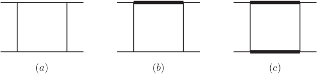
Figure 1: One-loop topologies. Thin lines represent massless external particles and propagators, while thick lines represent massive propagators.

We calculate the quantum corrections to the processes (1,2) using a Feynman diagrams approach. After considering the interference with the leading order, and summing over the spins and colors, we express the squared absolute value of the amplitude in terms of dimensionally regularized scalar integrals. These integrals are reduced to a set of MIs by means of integration-by-parts identities Tkachov:1981wb ; Chetyrkin:1981qh and Lorentz-invariance identities Gehrmann:1999as , implemented in the computer program Reduze 2 Studerus:2009ye ; vonManteuffel:2012np .

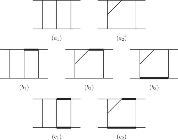
Figure 2: Two-loop topologies. Thin lines represent massless external particles and propagators, while thick lines represent massive propagators.

At one-loop, the topologies involved in the QCD and EW corrections are shown in figure 1, where we distinguish: $a)$ the mass-less case; $b)$ the exchange of one massive particle; and $c)$ the exchange of two massive particles.

At two-loop, the topologies required by the $\mathcal{O}(\alpha\alpha_{S})$ corrections are only planar. They are shown in figure 2. As for the one-loop case, we consider three classes of diagrams, according to the presence of massive particles.

Topologies $a_{1})$ and $a_{2})$ belong to the same 9-denominators mass-less topology. They reduce to 8 MIs, that were already known in the literature Gehrmann:1999as ; Smirnov:1999gc ; Tausk:1999vh ; Anastasiou:2000mf . Topologies $b_{1})$–$b_{3})$ have one massive propagator. They reduce to 31 MIs out of which 24 contain one massive propagator and 7 are part of the MIs for topologies $a_{1})$ and $a_{2})$. The three-point functions were already known in the literature Fleischer:1998nb ; Aglietti:2003yc ; Bonciani:2003hc . The four-point functions are calculated and presented here for the first time. Topologies $c_{1})$ and $c_{2})$ have two massive propagators and they reduce to 36 MIs, out of which 17 contain two massive propagators, 15 contain one massive propagator (and they are included in the set of MIs for topologies $b_{1})$–$b_{3})$) and 4 contain only massless propagators. The three-point functions were known in the literature Aglietti:2004tq ; Aglietti:2004ki and the four-point functions are presented here for the first time.

The routings for one- and two-mass topologies, at the one- and two-loop level, can be defined in terms of the following sets of denominators $D_{n}$, where $k_{i}$ ($i=1,2$) are the loop momenta, and $p_{i}$ ($i=1,\ldots,4$) are the external momenta:

• One-mass topologies. For the one-loop one-mass integrals (figure 1 $b)$, we have:

  $$D_{1}=k_{1}^{2},\quad D_{2}=(k_{1}-p_{1})^{2},\quad D_{3}=(k_{1}+p_{2})^{2}-m^{2},\quad D_{4}=(k_{1}-p_{1}+p_{3})^{2}.$$

  At two loops (figure 2 $b_{1}$–$b_{3}$), instead, we have:

  $$D_{1}=k_{1}^{2},\quad D_{2}=k_{2}^{2},\quad D_{3}=(k_{1}+k_{2})^{2},\quad D_{4}=(k_{1}-p_{1})^{2},$$

  $$D_{5}=(k_{1}+p_{2})^{2},\quad D_{6}=(k_{1}+k_{2}-p_{1})^{2}-m^{2},\quad D_{7}=(k_{1}+k_{2}+p_{2})^{2},$$

  $$D_{8}=(k_{1}+k_{2}-p_{1}+p_{3})^{2},\quad D_{9}=(k_{1}-p_{1}+p_{3})^{2}.$$ (7)

• Two-mass topologies. For the one-loop two-mass integrals (figure 1 $c)$, we have:

  $$D_{1}=k_{1}^{2},\quad D_{2}=(k_{1}-p_{1})^{2}-m^{2},\quad D_{3}=(k_{1}+p_{2})^{2}-m^{2},\quad D_{4}=(k_{1}-p_{1}+p_{3})^{2}.$$

  At two loops (figure 2 $c_{1}$ and $c_{2}$), instead, we have:

  $$D_{1}=k_{1}^{2},\quad D_{2}=k_{2}^{2},\quad D_{3}=(k_{1}+k_{2})^{2},\quad D_{4}=(k_{1}-p_{1})^{2},$$

  $$D_{5}=(k_{1}+p_{2})^{2},\quad D_{6}=(k_{1}+k_{2}-p_{1})^{2}-m^{2},\quad D_{7}=(k_{1}+k_{2}+p_{2})^{2}-m^{2},$$

  $$D_{8}=(k_{1}+k_{2}-p_{1}+p_{3})^{2},\quad D_{9}=(k_{1}-p_{1}+p_{3})^{2}.$$ (8)

In the following we consider $\ell$-loop Feynman integrals in $\mathrm{d}$ dimensions, built out of $p$ of the above denominators, each raised to some integer power, of the form

$$\int\widetilde{\mathrm{d}^{d}k_{1}}\ldots\widetilde{\mathrm{d}^{d}k_{\ell}}\,\frac{1}{D_{a_{1}}^{n_{1}}\ldots D_{a_{p}}^{n_{p}}},$$ (9)

where the integration measure is defined as

$$\widetilde{\mathrm{d}^{d}k_{i}}\equiv\frac{\mathrm{d}^{d}k_{i}}{(2\pi)^{d}}\left(\frac{i\,S_{\epsilon}}{16\pi^{2}}\right)^{-1}\left(\frac{m^{2}}{\mu^{2}}\right)^{\epsilon},$$ (10)

with $\mu$ the ’t Hooft scale of dimensional regularization, and

$$S_{\epsilon}\equiv(4\pi)^{\epsilon}\,\frac{\Gamma(1+\epsilon)\,\Gamma^{2}(1-\epsilon)}{\Gamma(1-2\epsilon)}\,.$$ (11)

In eqs. (10), (11) we used $\epsilon=(4-d)/2$.

3 System of Differential equations for Master Integrals

In this section, we describe the general structure of the systems of differential equations obeyed by the MIs, and the corresponding solutions. Sections dedicated to the one-mass and two-mass MIs will follow, where the details of their complete determination will be provided.

The $b$- and $c$-type MIs are functions of the Mandelstam invariants defined in eq. (3) and of the mass $m$. For their evaluation it is convenient to define the dimensionless ratios

$$x\equiv-\frac{s}{m^{2}},\quad y\equiv-\frac{t}{m^{2}},\quad z\equiv-\frac{u}{m^{2}},\quad\text{ with }\;x+y+z=0.$$ (12)

The $b$-type and $c$-type MIs obey systems of partial differential equations in $x$ and $y$, which can be combined into matrix equations for their total differentials. In general, the vector of MIs $\mathbf{F}$ is solution of the following system of differential equation,

$$d\mathbf{F}=d\mathbb{K}\,\mathbf{F}\ ,$$ (13)

where the matrix $\mathbb{K}$ depends both on the kinematic variables and on the spacetime dimension $d=4-2\epsilon$.

By means of a suitable basis transformation, built with the help of the Magnus exponential Magnus ; Argeri:2014qva following the procedure outlined in Sec. 2 of DiVita:2014pza , we obtain a canonical set of MIs Henn:2013pwa . Such a basis obeys a system of differential equation where the dependence on $\epsilon$ is factorized from the kinematics. Moreover, the coefficient matrices can be assembled in a (logarithmic) differential form, referred to as canonical $\operatorname{\mathit{d}log}$-form. Hence, the canonical basis $\mathbf{I}$ obeys the following system of equations,

$$d\mathbf{I}=\epsilon\,d\mathbb{A}\,\mathbf{I}\ ,$$ (14)

with

$$d\mathbb{A}=\sum_{i=1}^{n}\mathbb{M}_{i}\,\operatorname{\mathit{d}log}\eta_{i}\,,$$ (15)

where $d\mathbb{A}$ is the $\operatorname{\mathit{d}log}$ matrix written in terms of differentials $\operatorname{\mathit{d}log}\eta_{i}$ (that contain the kinematic dependence) and coefficient matrices $\mathbb{M}_{i}$ (with rational-number entries). The integrability conditions for eq. (14) read

$$\partial_{a}\partial_{b}\mathbb{A}-\partial_{b}\partial_{a}\mathbb{A}=0\,,\qquad[\partial_{a}\mathbb{A},\partial_{b}\mathbb{A}]=0\,.$$ (16)

3.1 General solution

The general solution of the canonical system of differential equations (14) can be compactly written at a point $\vec{x}=(x^{1},x^{2})=(x,y)$ as

$$\mathbf{I}(\epsilon,\vec{x})={} \mathcal{P}\exp\left\{\epsilon\int_{\gamma}d\mathbb{A}\right\}\mathbf{I}(\epsilon,\vec{x}_{0})\,,$$ (17)

where $\mathbf{I}(\epsilon,\vec{x}_{0})$ is a vector of arbitrary constants, depending on $\epsilon$, while $d\mathbb{A}$ depends only on the kinematic variables. In the above expression, the path-ordered exponential is a short notation for the series

$$\mathcal{P}\exp\left\{\epsilon\int_{\gamma}d\mathbb{A}\right\}=\mathbbm{1}+\epsilon\int_{\gamma}d\mathbb{A}+\epsilon^{2}\int_{\gamma}d\mathbb{A}\,d\mathbb{A}+\epsilon^{3}\int_{\gamma}d\mathbb{A}\,d\mathbb{A}\,d\mathbb{A}\ldots\,,$$ (18)

in which the line integral of the product of $k$ matrix-valued 1-forms $d\mathbb{A}$ is understood in the sense of Chen’s iterated integrals Chen:1977oja (see also Brown:2009qja and the pedagogical lectures Brown:2009lectures ) and $\gamma$ is a piecewise-smooth path

$$\gamma:[0,1]\ni t\mapsto\gamma(t)=(\gamma^{1}(t),\gamma^{2}(t))\,,$$ (19)

such that $\gamma(0)=\vec{x}_{0}$ and $\gamma(1)=\vec{x}$. It follows from Chen’s theorem that the iterated integrals in eq. (18) do not depend on the actual choice of the path, provided the curve does not contain any singularity of $d\mathbb{A}$ and it does not cross any of its branch cuts, but only on the endpoints. In this sense, if one fixes $\vec{x}_{0}$ and lets $\vec{x}$ vary, eq. (17) can be thought of as a function of $\vec{x}$. In the limit $\vec{x}\to\vec{x}_{0}$, the line shrinks to a point and all the path integrals in eq.(18) vanish, so that $\mathbf{I}(\epsilon,\vec{x})\to\mathbf{I}(\epsilon,\vec{x}_{0})$, i.e. the integration constants have a natural interpretation as initial values, and the path-ordered exponential as evolution operator. We assume that the vector of MIs at any point $\mathbf{I}(\vec{x})$ is normalized in such a way that it admits a Taylor series in $\epsilon$:

$$\mathbf{I}(\epsilon,\vec{x})=\mathbf{I}^{(0)}(\vec{x})+\epsilon\,\mathbf{I}^{(1)}(\vec{x})+\epsilon^{2}\mathbf{I}^{(2)}(\vec{x})+\ldots\,.$$ (20)

The solution $\mathbf{I}(\epsilon,\vec{x})$ is then in principle determined through (17) at any order of the $\epsilon$-expansion, and reads (up to the coefficient of $\epsilon^{4}$)

$$\mathbf{I}^{(0)}(\vec{x})={} \mathbf{I}^{(0)}(\vec{x}_{0})\,,$$ (21)

$$\mathbf{I}^{(1)}(\vec{x})={} \mathbf{I}^{(1)}(\vec{x}_{0})+\int_{\gamma}d\mathbb{A}\;\mathbf{I}^{(0)}(\vec{x}_{0})\,,$$ (22)

$$\mathbf{I}^{(2)}(\vec{x})={} \mathbf{I}^{(2)}(\vec{x}_{0})+\int_{\gamma}d\mathbb{A}\;\mathbf{I}^{(1)}(\vec{x}_{0})+\int_{\gamma}d\mathbb{A}\;d\mathbb{A}\;\mathbf{I}^{(0)}(\vec{x}_{0})\,,$$ (23)

$$\mathbf{I}^{(3)}(\vec{x})={} \mathbf{I}^{(3)}(\vec{x}_{0})+\int_{\gamma}d\mathbb{A}\;\mathbf{I}^{(2)}(\vec{x}_{0})\,,+\int_{\gamma}d\mathbb{A}\;d\mathbb{A}\;\mathbf{I}^{(1)}(\vec{x}_{0})$$

$$+\int_{\gamma}d\mathbb{A}\;d\mathbb{A}\;d\mathbb{A}\;\mathbf{I}^{(0)}(\vec{x}_{0})\,,$$ (24)

$$\mathbf{I}^{(4)}(\vec{x})={} \mathbf{I}^{(4)}(\vec{x}_{0})+\int_{\gamma}d\mathbb{A}\;\mathbf{I}^{(3)}(\vec{x}_{0})+\int_{\gamma}d\mathbb{A}\;d\mathbb{A}\;\mathbf{I}^{(2)}(\vec{x}_{0})$$

$$+\int_{\gamma}d\mathbb{A}\;d\mathbb{A}\;d\mathbb{A}\;\mathbf{I}^{(1)}(\vec{x}_{0})+\int_{\gamma}d\mathbb{A}\;d\mathbb{A}\;d\mathbb{A}\;d\mathbb{A}\;\mathbf{I}^{(0)}(\vec{x}_{0})\,.$$ (25)

The problem of solving (14), given a set of initial conditions $\mathbf{I}(\vec{x}_{0})$, reduces therefore to the evaluation of matrices of the type

$$\int_{\gamma}\underbrace{d\mathbb{A}\ldots d\mathbb{A}}_{\text{k times}}\,,$$ (26)

whose entries, due to (15), are linear combinations of Chen’s iterated integrals of the form

$$\int_{\gamma}\operatorname{\mathit{d}log}\eta_{i_{k}}\ldots\operatorname{\mathit{d}log}\eta_{i_{1}}\equiv{} \int_{0\leq t_{1}\leq\ldots\leq t_{k}\leq 1}g^{\gamma}_{i_{k}}(t_{k})\ldots g^{\gamma}_{i_{1}}(t_{1})\,dt_{1}\ldots\,dt_{k}\,,$$ (27)

with

$$g^{\gamma}_{i}(t)={} \frac{d}{dt}\log\eta_{i}(\gamma(t))\,.$$ (28)

We refer to the number of iterated integrations $k$ as the weight of the path-integral. The empty integral (eq. (27) for $k=0$) is defined to be equal to 1. We stress that only the matrices (26) do not depend on the explicit choice of the path. The individual summands of the form in eq. (27), which contribute to their entries, in general depend on such a choice. To keep the notation compact, we define

$$\mathcal{C}_{i_{k},\ldots,i_{1}}^{\,[\gamma]}\equiv\int_{\gamma}\operatorname{\mathit{d}log}\eta_{i_{k}}\ldots\operatorname{\mathit{d}log}\eta_{i_{1}}\,,$$ (29)

which also emphasizes that the iterated integrals in (27) are in general functionals of the path $\gamma$.

3.2 Properties of Chen’s iterated integrals

The general theory of iterated path integrals was developed by Chen Chen:1977oja . Chen’s iterated integrals satisfy a number of properties that we summarize for completeness:

• Invariance under path reparametrization. The integral $\mathcal{C}_{i_{k},\ldots,i_{1}}^{\,[\gamma]}$ does not depend on how one chooses to parametrize the path $\gamma$.

• Reverse path formula. If the path $\gamma^{-1}$ is the path $\gamma$ traversed in the opposite direction, then

  $$\mathcal{C}_{i_{k},\ldots,i_{1}}^{\,[\gamma^{-1}]}=(-1)^{k}\mathcal{C}_{i_{k},\ldots,i_{1}}^{\,[\gamma]}\,.$$ (30)

• Recursive structure. From (27) and (28) it follows that the line integral of one $\operatorname{\mathit{d}log}$ is defined as usual

  $$\int_{\gamma}\operatorname{\mathit{d}log}\eta\equiv{} \int_{0\leq t\leq 1}\frac{\operatorname{\mathit{d}log}\eta(\gamma(t))}{dt}dt\,,$$ (31)

  and only depends on the endpoints $\vec{x}_{0},\vec{x}$

  $$\int_{\gamma}\operatorname{\mathit{d}log}\eta=\log{\eta(\vec{x})}-\log\eta(\vec{x}_{0})\,.$$ (32)

  It is convenient to introduce the path integral “up to some point along $\gamma$”: given a path $\gamma$ and a parameter $s\in[0,1]$, one can define the 1-parameter family of paths

  $$\gamma_{s}:[0,1]\ni t\mapsto\vec{x}=(\gamma^{1}(s\,t),\gamma^{2}(s\,t))\,.$$ (33)

  If $s=1$, then trivially $\gamma_{s}=\gamma$. If $s=0$ the image of the interval $[0,1]$ is just $\{\vec{x}_{0}\}$. If $s\in(0,1)$, then the curve $\gamma_{s}([0,1])$ starts at $\gamma(0)=\vec{x}_{0}$ and overlaps with the curve $\gamma([0,1])$ up to the point $\gamma(s)$, where it ends. It is then easy to see that the path integral along $\gamma_{s}$ can be written as

  $$\mathcal{C}_{i_{k},\ldots,i_{1}}^{\,[\gamma_{s}]}=\int_{0\leq t_{1}\leq\ldots\leq t_{k}\leq s}g^{\gamma}_{i_{k}}(t_{k})\ldots g^{\gamma}_{i_{1}}(t_{1})\,dt_{1}\ldots\,dt_{k}\,,$$ (34)

  which differs from eq. (27) by the fact that the outer integration (i.e. the one in $dt_{k}$) is performed over $[0,s]$ instead of $[0,1]$. Having introduced $\gamma_{s}$, we can rewrite (27) in a recursive manner:

  $$\mathcal{C}_{i_{k},\ldots,i_{1}}^{\,[\gamma]}={} \int_{0}^{1}g^{\gamma}_{i_{k}}(s)\,\mathcal{C}_{i_{k-1},\ldots,i_{1}}^{\,[\gamma_{s}]}ds\,.$$ (35)

  From eq. (34) we can also immediately derive the following identity:

  $$\frac{d}{ds}\,\mathcal{C}_{i_{k},\ldots,i_{1}}^{\,[\gamma_{s}]}=g^{\gamma}_{i_{k}}(s)\,\mathcal{C}_{i_{k-1},\ldots,i_{1}}^{\,[\gamma_{s}]}\,.$$ (36)

• Shuffle algebra. Chen’s iterated integrals fulfill shuffle algebra relations: if $\vec{m}=m_{M},\ldots,m_{1}$ and $\vec{n}=n_{N},\ldots,n_{1}$ (with $M$ and $N$ natural numbers)

  $$\mathcal{C}_{\vec{m}}^{\,[\gamma]}\,\mathcal{C}_{\vec{n}}^{\,[\gamma]}={} \sum_{\text{shuffles }\sigma}\mathcal{C}_{\sigma(m_{M}),\ldots,\sigma(m_{1}),\sigma(n_{N}),\ldots,\sigma(n_{1})}^{\,[\gamma]}\,,$$ (37)

  where the sum runs over all the permutations $\sigma$ that preserve the relative order of $\vec{m}$ and $\vec{n}$.

• Path composition formula. If $\alpha,\beta:[0,1]\to\mathcal{M}$ are such that $\alpha(0)=\vec{x}_{0}$, $\alpha(1)=\beta(0)$, and $\beta(1)=\vec{x}$, then the composed path $\gamma\equiv\alpha\beta$ is obtained by first traversing $\alpha$ and then $\beta$. One can prove that the integral over such a composed path satisfies

  $$\mathcal{C}_{i_{k},\ldots,i_{1}}^{\,[\alpha\beta]}=\sum_{p=0}^{k}\mathcal{C}_{i_{k},\ldots,i_{p+1}}^{\,[\beta]}\,\mathcal{C}_{i_{p},\ldots,i_{1}}^{\,[\alpha]}\,.$$ (38)

• Integration-by-parts formula. In order to compute the path ordered integral of $k$ $\operatorname{\mathit{d}log}$ forms using the definition, eq. (27) (or, equivalently, eq. (35)), in principle one would have to perform $k$ nested integrations. When a fully analytic solution cannot be achieved, numerical integration can as well be employed. Therefore one can use an alternative form of the Chen iterated integral suitable for the combined use of analytic and numerical integrations. In fact, we observe that the innermost integration can always be performed analytically using (31), so that only $k-1$ integrations are left. For instance, in the case $k=2$,

  $$\mathcal{C}_{b,a}^{\,[\gamma]}={} \int_{0}^{1}g_{b}(t)\,\mathcal{C}_{a}^{\,[\gamma_{t}]}\,dt$$

  $$={} \int_{0}^{1}g_{b}(t)(\log\eta_{a}(\vec{x}(t))-\log\eta_{a}(\vec{x}_{0}))\,dt\,.$$ (39)

  For $k\geq 3$, one can proceed recursively using eq. (35), assuming that the numerical evaluation up to the first $k-1$ iterations is a solved problem. Using integration by parts, one can show that the numerical integration over the outermost weight $g_{k}$ can actually be avoided, leaving only $k-2$ integrations to be performed

  $$\mathcal{C}_{i_{k},\ldots,i_{1}}^{\,[\gamma]}={} \log\eta_{i_{k}}(\vec{x})\,\mathcal{C}_{i_{k-1},\ldots,i_{1}}^{\,[\gamma]}-\int_{0}^{1}\log\eta_{i_{k}}(\vec{x}(t))\,g_{i_{k-1}}(t)\,\mathcal{C}_{i_{k-2},\ldots,i_{1}}^{\,[\gamma_{t}]}dt\,.$$ (40)

3.3 Mixed Chen-Goncharov representation

In principle eq. (17) completely determines the solution, which can be written in terms of Chen’s iterated integrals along an arbitrary piecewise-smooth path (see the discussion below eq. (17)). The initial conditions $\mathbf{I}(\vec{x}_{0})$ can be computed analytically, if possible, or by means of numerical methods. The number of iterated integrals that have to be evaluated numerically can be minimized by the use the of algebraic identities relating them. According to the discussion in section 3.2, the evaluation of the solution up to weight 4 requires in general 2 nested numerical integrations.

In order to obtain results that allow for an efficient numerical evaluation, we have chosen to give the solution in a mixed representation that involves GPLs and general Chen’s iterated integrals. The representation in terms of GPLs is particularly convenient because public packages exist, like GiNaC, that implement their numerical evaluation in a fast and accurate way. Whenever the alphabet is rational in the kinematic variables $x_{i}$, one can always choose a path that allows to express the Chen iterated integrals in terms of GPLs, namely the broken line such that, in each segment, only one of the $x_{i}$ is allowed to vary. Along each segment, by means of factorization over the complex numbers, one can obtain a linear alphabet and, therefore, the GPLs representation. This approach is equivalent to integrating the differential equations for $x$ and $y$ separately. By integrating, say, the equation in $x$ one obtains the solution in terms of GPLs of argument $x$ up to an unknown function $\mathbf{H}(y)$. By taking the derivative with respect to $y$ and matching to the equation in $y$, one obtains a differential equation for $\mathbf{H}(y)$. The latter can be again integrated in terms of GPLs of argument $y$, up to a constant.

As we will discuss in section 5, the alphabet for our differential equations is not always rational in the kinematic variables we use and, in that case, a representation in terms of GPLs cannot be given for the complete solution. To reach the mixed representation, we have exploited the property of path-independence of the coefficients of the $\epsilon$-expansion of the solution eq. (17). In particular, eqs. (22)-(25) can be written in an equivalent alternative form using eq. (35):

$$\mathbf{I}^{(k)}(\vec{x})={} \mathbf{I}^{(k)}(\vec{x}_{0})+\int_{0}^{1}\Bigg{[}\frac{d\mathbb{A}(t)}{dt}\mathbf{I}^{(k-1)}(\vec{x}_{t})\Bigg{]}dt\,,$$ (41)

where $\vec{x}_{t}$ is the point $(x(t),y(t))$ along the curve identified by $\gamma$. We see that, in order to build the weight-$k$ coefficient, one must perform a path integration over the weight-$(k-1)$ coefficient. The choice of such path is independent of the path used to compute the former because, as we have already discussed, each coefficient is a function of the sole endpoints. In other words, as far as the weight-$k$ coefficient of the solution is concerned, we are free to choose the integration path independently for each of the $k$ integrations (for each component of $\mathbf{I}(\vec{x})$).

To see how this can be useful in our computation, we note that the letters $\eta_{i}$ (in suitable variables, say $\vec{x}$) can be grouped in two classes. The first contains the letters that are rational in the components of $\vec{x}$ and happens to represent the alphabet for most of the MIs we need to compute. The second is the class of letters that are non-rational functions of the variables. The two classes together constitute the alphabet for the 5 most complicated MIs.

Starting from the weight-1 coefficient of the solution, we proceed as follows. As far as the involved $\eta_{i}$’s belong to the first class of letters, we can express the solution in terms of GPLs. We keep integrating in this manner until, at some weight $k$, the solution begins to involve non-rational $\eta_{i}$’s. At this point we proceed with the path integration as in (41). Within this approach, the weight $k-1$ solution is not expressed in terms of Chen’s iterated integrals over an arbitrary path, but in terms of GPLs. We introduce the following notation to keep our results compact:

$$\mathcal{C}_{a|\vec{m}|\vec{n}}^{\,[\gamma]}\equiv{} \int_{0}^{1}\,g_{a}^{\gamma}(t)\,G^{\gamma}_{\vec{m}}(x)\,G^{\gamma}_{\vec{n}}(y)\,dt\,,$$ (42)

$$\mathcal{C}_{a|\vec{m}|\scalebox{0.5}{\mbox{$\displaystyle\varnothing$}}}^{\,[\gamma]}\equiv{} \int_{0}^{1}\,g_{a}^{\gamma}(t)\,G^{\gamma}_{\vec{m}}(x)\,dt\,,$$ (43)

$$\mathcal{C}_{a|\scalebox{0.5}{\mbox{$\displaystyle\varnothing$}}|\vec{n}}^{\,[\gamma]}\equiv{} \int_{0}^{1}\,g_{a}^{\gamma}(t)\,G^{\gamma}_{\vec{n}}(y)\,dt\,,$$ (44)

$$\mathcal{C}_{a,\vec{b}|\vec{m}|\vec{n}}^{\,[\gamma]}\equiv{} \int_{0}^{1}\,g_{a}^{\gamma}(t)\,\mathcal{C}_{\vec{b}|\vec{m}|\vec{n}}^{\,[\gamma_{t}]}\,dt\,,$$ (45)

where $G^{\gamma}_{\vec{m}}(x)$ and $G^{\gamma}_{\vec{n}}(y)$ stand for the GPLs $G_{\vec{m}}(x)$ and $G_{\vec{n}}(y)$ evaluated at $(x,y)=(\gamma^{1}(t),\gamma^{2}(t))$.

3.4 Constant GPLs

In the determination of the boundary values of the MIs we encountered constant GPLs of argument $1$ with weights drawn from three sets. For the one-mass MIs there is only one relevant set, with four weights,

• $\{-1,0,\frac{1}{2},1\}$ .

For the two-mass MIs we encountered the following two sets, with seven weights each

• $\{-1,0,-i,i,1,(-1)^{\frac{1}{3}},-(-1)^{\frac{2}{3}}\}$,

• $\{-1,0,-i,i,1,-(-1)^{\frac{1}{6}},-(-1)^{\frac{5}{6}}\}$,

where the former includes the third roots of $-1$ and the latter involves a subset of the sixth roots of $-1$. With the help of GiNaC, we verified that, at order $\epsilon^{k}$, the Taylor coefficient of each MI $\text{I}_{i}^{(k)}$ contains a combinations of constant GPLs that turns out to be proportional to $\zeta_{k}$, namely amounting to $q_{i,k}\ \zeta_{k}$, with $q_{i,k}\in\mathbb{Q}$. The resulting identities were verified at high numerical accuracy. As examples, we show,

$$0={} G_{r}+G_{-r^{2}}\,,$$ (46)

$$\zeta_{2}={} 3G_{0,-r^{2}}+4G_{r,-r^{2}}+4G_{-r^{2},0}-2G_{-r^{2},1}+4G_{-r^{2},r}$$

$$+4G_{-r^{2},-r^{2}}+3G_{0,r}+4G_{r,0}-2G_{r,1}+4G_{r,r}\,,$$ (47)

$$-\frac{77}{8}\zeta_{3}={} G_{-1,-1,\frac{1}{2}}+G_{-1,\frac{1}{2},-1}+G_{-1,\frac{1}{2},1}+3G_{0,0,\frac{1}{2}}+3G_{0,\frac{1}{2},1}+G_{\frac{1}{2},-1,-1}$$

$$+G_{\frac{1}{2},-1,1}-G_{\frac{1}{2},0,\frac{1}{2}}+4G_{\frac{1}{2},0,1}+G_{\frac{1}{2},1,-1}+\frac{3}{2}\zeta_{2}G_{\frac{1}{2}}\,,$$ (48)

where for simplicity we omitted the argument ($x=1$) of the GPLs and we defined the weight $r\equiv(-1)^{1/3}$. For related studies see also Broadhurst:1998rz ; 2007arXiv0707.1459Z ; Moriello ; Henn:2015sem .

4 One-mass Master Integrals

In this section we describe the computation of the MIs with one internal massive line, namely topology $(b)$ of figure 1 and topologies $(b_{1})$-$(b_{3})$ of figure 2.

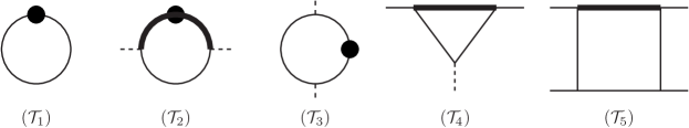
Figure 3: One-loop one-mass MIs $\mathcal{T}_{1,\ldots,5}$. Thin lines represent massless external particles and propagators; thick lines stand for massive propagators; an horizontal (vertical) dashed external line represents an off-shell leg with squared momentum equal to $s$ ($t$); dots indicate squared propagators.

4.1 One-loop

The following set of MIs for the one-loop one-mass box obeys a differential equation in $x$ and $y$, defined in eq. (12), which is linear in $\epsilon$:

$$\text{F}_{1} =\epsilon\,\mathcal{T}_{1}\,, \text{F}_{2} =\epsilon\,\mathcal{T}_{2}\,, \text{F}_{3} =\epsilon\,\mathcal{T}_{3}\,,$$

$$\text{F}_{4} =\epsilon^{2}\,\mathcal{T}_{4}\,, \text{F}_{5} =\epsilon^{2}\,\mathcal{T}_{5}\,.$$ (49)

where the $\mathcal{T}_{i}$ are depicted in figure 3. By means of the Magnus exponential Magnus ; Argeri:2014qva , according to the procedure outlined in Sec. 2 of DiVita:2014pza , we obtain the canonical MIs

$$\text{I}_{1} =\text{F}_{1}\,, \text{I}_{2} =-s\,\text{F}_{2}\,, \text{I}_{3} =-t\,\text{F}_{3}\,,$$

$$\text{I}_{4} =-t\,\text{F}_{4}\,, \text{I}_{5} =(s-m^{2})\,t\,\text{F}_{5}\,.$$ (50)

The alphabet of the corresponding $\operatorname{\mathit{d}log}$-form, eq (15), is

$$\eta_{1} =x\,, \eta_{2} =1+x\,, \eta_{3} =y\,,$$

$$\eta_{4} =1-y\,, \eta_{5} =x+y\,,$$ (51)

and the coefficient matrices read

$$\begin{aligned} \mathbb{M}_{1}&=\scalebox{0.6}{\mbox{$\displaystyle\left(\begin{array}[]{ccccc}\hphantom{\scalebox{0.5}[1.0]{$-$}}0&\hphantom{\scalebox{0.5}[1.0]{$-$}}0&\hphantom{\scalebox{0.5}[1.0]{$-$}}0&\hphantom{\scalebox{0.5}[1.0]{$-$}}0&\hphantom{\scalebox{0.5}[1.0]{$-$}}0\\ \hphantom{\scalebox{0.5}[1.0]{$-$}}0&\hphantom{\scalebox{0.5}[1.0]{$-$}}1&\hphantom{\scalebox{0.5}[1.0]{$-$}}0&\hphantom{\scalebox{0.5}[1.0]{$-$}}0&\hphantom{\scalebox{0.5}[1.0]{$-$}}0\\ \hphantom{\scalebox{0.5}[1.0]{$-$}}0&\hphantom{\scalebox{0.5}[1.0]{$-$}}0&\hphantom{\scalebox{0.5}[1.0]{$-$}}0&\hphantom{\scalebox{0.5}[1.0]{$-$}}0&\hphantom{\scalebox{0.5}[1.0]{$-$}}0\\ \hphantom{\scalebox{0.5}[1.0]{$-$}}0&\hphantom{\scalebox{0.5}[1.0]{$-$}}0&\hphantom{\scalebox{0.5}[1.0]{$-$}}0&\hphantom{\scalebox{0.5}[1.0]{$-$}}0&\hphantom{\scalebox{0.5}[1.0]{$-$}}0\\ \hphantom{\scalebox{0.5}[1.0]{$-$}}0&\hphantom{\scalebox{0.5}[1.0]{$-$}}2&\scalebox{0.5}[1.0]{$-$}1&\scalebox{0.5}[1.0]{$-$}1&\hphantom{\scalebox{0.5}[1.0]{$-$}}1\\ \end{array}\right)$}}\,,&\qquad\mathbb{M}_{2}&=\scalebox{0.6}{\mbox{$\displaystyle\left(\begin{array}[]{ccccc}\hphantom{\scalebox{0.5}[1.0]{$-$}}0&\hphantom{\scalebox{0.5}[1.0]{$-$}}0&\hphantom{\scalebox{0.5}[1.0]{$-$}}0&\hphantom{\scalebox{0.5}[1.0]{$-$}}0&\hphantom{\scalebox{0.5}[1.0]{$-$}}0\\ \scalebox{0.5}[1.0]{$-$}1&\scalebox{0.5}[1.0]{$-$}2&\hphantom{\scalebox{0.5}[1.0]{$-$}}0&\hphantom{\scalebox{0.5}[1.0]{$-$}}0&\hphantom{\scalebox{0.5}[1.0]{$-$}}0\\ \hphantom{\scalebox{0.5}[1.0]{$-$}}0&\hphantom{\scalebox{0.5}[1.0]{$-$}}0&\hphantom{\scalebox{0.5}[1.0]{$-$}}0&\hphantom{\scalebox{0.5}[1.0]{$-$}}0&\hphantom{\scalebox{0.5}[1.0]{$-$}}0\\ \hphantom{\scalebox{0.5}[1.0]{$-$}}0&\hphantom{\scalebox{0.5}[1.0]{$-$}}0&\hphantom{\scalebox{0.5}[1.0]{$-$}}0&\hphantom{\scalebox{0.5}[1.0]{$-$}}0&\hphantom{\scalebox{0.5}[1.0]{$-$}}0\\ \hphantom{\scalebox{0.5}[1.0]{$-$}}0&\hphantom{\scalebox{0.5}[1.0]{$-$}}0&\hphantom{\scalebox{0.5}[1.0]{$-$}}0&\hphantom{\scalebox{0.5}[1.0]{$-$}}0&\scalebox{0.5}[1.0]{$-$}2\\ \end{array}\right)$}}\,,&\qquad\mathbb{M}_{3}&=\scalebox{0.6}{\mbox{$\displaystyle\left(\begin{array}[]{ccccc}\hphantom{\scalebox{0.5}[1.0]{$-$}}0&\hphantom{\scalebox{0.5}[1.0]{$-$}}0&\hphantom{\scalebox{0.5}[1.0]{$-$}}0&\hphantom{\scalebox{0.5}[1.0]{$-$}}0&\hphantom{\scalebox{0.5}[1.0]{$-$}}0\\ \hphantom{\scalebox{0.5}[1.0]{$-$}}0&\hphantom{\scalebox{0.5}[1.0]{$-$}}0&\hphantom{\scalebox{0.5}[1.0]{$-$}}0&\hphantom{\scalebox{0.5}[1.0]{$-$}}0&\hphantom{\scalebox{0.5}[1.0]{$-$}}0\\ \hphantom{\scalebox{0.5}[1.0]{$-$}}0&\hphantom{\scalebox{0.5}[1.0]{$-$}}0&\scalebox{0.5}[1.0]{$-$}1&\hphantom{\scalebox{0.5}[1.0]{$-$}}0&\hphantom{\scalebox{0.5}[1.0]{$-$}}0\\ \hphantom{\scalebox{0.5}[1.0]{$-$}}0&\hphantom{\scalebox{0.5}[1.0]{$-$}}0&\hphantom{\scalebox{0.5}[1.0]{$-$}}0&\hphantom{\scalebox{0.5}[1.0]{$-$}}1&\hphantom{\scalebox{0.5}[1.0]{$-$}}0\\ \hphantom{\scalebox{0.5}[1.0]{$-$}}0&\hphantom{\scalebox{0.5}[1.0]{$-$}}0&\hphantom{\scalebox{0.5}[1.0]{$-$}}0&\hphantom{\scalebox{0.5}[1.0]{$-$}}0&\scalebox{0.5}[1.0]{$-$}1\\ \end{array}\right)$}}\,,&\end{aligned}$$

$$\begin{aligned} \mathbb{M}_{4}&=\scalebox{0.6}{\mbox{$\displaystyle\left(\begin{array}[]{ccccc}\hphantom{\scalebox{0.5}[1.0]{$-$}}0&\hphantom{\scalebox{0.5}[1.0]{$-$}}0&\hphantom{\scalebox{0.5}[1.0]{$-$}}0&\hphantom{\scalebox{0.5}[1.0]{$-$}}0&\hphantom{\scalebox{0.5}[1.0]{$-$}}0\\ \hphantom{\scalebox{0.5}[1.0]{$-$}}0&\hphantom{\scalebox{0.5}[1.0]{$-$}}0&\hphantom{\scalebox{0.5}[1.0]{$-$}}0&\hphantom{\scalebox{0.5}[1.0]{$-$}}0&\hphantom{\scalebox{0.5}[1.0]{$-$}}0\\ \hphantom{\scalebox{0.5}[1.0]{$-$}}0&\hphantom{\scalebox{0.5}[1.0]{$-$}}0&\hphantom{\scalebox{0.5}[1.0]{$-$}}0&\hphantom{\scalebox{0.5}[1.0]{$-$}}0&\hphantom{\scalebox{0.5}[1.0]{$-$}}0\\ \scalebox{0.5}[1.0]{$-$}1&\hphantom{\scalebox{0.5}[1.0]{$-$}}0&\hphantom{\scalebox{0.5}[1.0]{$-$}}1&\scalebox{0.5}[1.0]{$-$}1&\hphantom{\scalebox{0.5}[1.0]{$-$}}0\\ \scalebox{0.5}[1.0]{$-$}1&\hphantom{\scalebox{0.5}[1.0]{$-$}}0&\hphantom{\scalebox{0.5}[1.0]{$-$}}1&\scalebox{0.5}[1.0]{$-$}1&\hphantom{\scalebox{0.5}[1.0]{$-$}}0\\ \end{array}\right)$}}\,,&\qquad\mathbb{M}_{5}&=\scalebox{0.6}{\mbox{$\displaystyle\left(\begin{array}[]{ccccc}\hphantom{\scalebox{0.5}[1.0]{$-$}}0&\hphantom{\scalebox{0.5}[1.0]{$-$}}0&\hphantom{\scalebox{0.5}[1.0]{$-$}}0&\hphantom{\scalebox{0.5}[1.0]{$-$}}0&\hphantom{\scalebox{0.5}[1.0]{$-$}}0\\ \hphantom{\scalebox{0.5}[1.0]{$-$}}0&\hphantom{\scalebox{0.5}[1.0]{$-$}}0&\hphantom{\scalebox{0.5}[1.0]{$-$}}0&\hphantom{\scalebox{0.5}[1.0]{$-$}}0&\hphantom{\scalebox{0.5}[1.0]{$-$}}0\\ \hphantom{\scalebox{0.5}[1.0]{$-$}}0&\hphantom{\scalebox{0.5}[1.0]{$-$}}0&\hphantom{\scalebox{0.5}[1.0]{$-$}}0&\hphantom{\scalebox{0.5}[1.0]{$-$}}0&\hphantom{\scalebox{0.5}[1.0]{$-$}}0\\ \hphantom{\scalebox{0.5}[1.0]{$-$}}0&\hphantom{\scalebox{0.5}[1.0]{$-$}}0&\hphantom{\scalebox{0.5}[1.0]{$-$}}0&\hphantom{\scalebox{0.5}[1.0]{$-$}}0&\hphantom{\scalebox{0.5}[1.0]{$-$}}0\\ \hphantom{\scalebox{0.5}[1.0]{$-$}}0&\scalebox{0.5}[1.0]{$-$}2&\scalebox{0.5}[1.0]{$-$}1&\hphantom{\scalebox{0.5}[1.0]{$-$}}1&\hphantom{\scalebox{0.5}[1.0]{$-$}}1\\ \end{array}\right)$}}\,.\end{aligned}$$ (52)

If $x>0$ and $0<y<1$ all the letters $\eta_{i}$ are positive. Since the alphabet is linear in $x$ and $y$, according to the discussion in section 3.3, the solution can be conveniently cast in terms of GPLs.

Instead of choosing a particular basepoint $\vec{x}_{0}$, the integration constants of $\text{I}_{2\dots 5}$ can be easily fixed by demanding regularity at the pseudothresholds $t\rightarrow-m^{2}$, $u\rightarrow 0$, $s\rightarrow 0$ and their reality in the euclidean region. On the other hand, $\text{I}_{1}$ is a constant and must be determined by direct integration:

$$\text{I}_{1} =\frac{\Gamma(1-2\epsilon)}{\Gamma(1-\epsilon)^{2}}\,.$$ (53)

4.2 Two-loop

At the two-loop order, the following set of MIs admits $\epsilon$-linear differential equations in $x$ and $y$ (defined in eq. (12)):

$$\text{F}_{1} =(1-\epsilon)\epsilon^{2}\,\mathcal{T}_{1}\,, \text{F}_{2} =\epsilon^{2}\,\mathcal{T}_{2}\,, \text{F}_{3} =\epsilon^{2}\,\mathcal{T}_{3}\,,$$

$$\text{F}_{4} =\epsilon^{2}\,\mathcal{T}_{4}\,, \text{F}_{5} =\epsilon^{2}\,\mathcal{T}_{5}\,, \text{F}_{6} =\epsilon^{2}\,\mathcal{T}_{6}\,,$$

$$\text{F}_{7} =\epsilon^{3}\,\mathcal{T}_{7}\,, \text{F}_{8} =\epsilon^{3}\,\mathcal{T}_{8}\,, \text{F}_{9} =\epsilon^{3}\,\mathcal{T}_{9}\,,$$

$$\text{F}_{10} =\epsilon^{2}\,\mathcal{T}_{10}\,, \text{F}_{11} =\epsilon^{2}\,\mathcal{T}_{11}\,, \text{F}_{12} =\epsilon^{3}\,\mathcal{T}_{12}\,,$$

$$\text{F}_{13} =\epsilon^{4}\,\mathcal{T}_{13}\,, \text{F}_{14} =\epsilon^{3}\,\mathcal{T}_{14}\,, \text{F}_{15} =\epsilon^{4}\,\mathcal{T}_{15}\,,$$

$$\text{F}_{16} =\epsilon^{3}\,\mathcal{T}_{16}\,, \text{F}_{17} =\epsilon^{3}\,\mathcal{T}_{17}\,, \text{F}_{18} =\epsilon^{4}\,\mathcal{T}_{18}\,,$$

$$\text{F}_{19} =\epsilon^{3}\,\mathcal{T}_{19}\,, \text{F}_{20} =\epsilon^{4}\,\mathcal{T}_{20}\,, \text{F}_{21} =\epsilon^{3}\,\mathcal{T}_{21}\,,$$

$$\text{F}_{22} =\epsilon^{4}\,\mathcal{T}_{22}\,, \text{F}_{23} =\epsilon^{3}\,\mathcal{T}_{23}\,, \text{F}_{24} =(1-2\epsilon)\epsilon^{3}\,\mathcal{T}_{24}\,,$$

$$\text{F}_{25} =\epsilon^{3}\,\mathcal{T}_{25}\,, \text{F}_{26} =\epsilon^{3}\,\mathcal{T}_{26}\,, \text{F}_{27} =\epsilon^{4}\,\mathcal{T}_{27}\,,$$

$$\text{F}_{28} =\epsilon^{3}\,\mathcal{T}_{28}\,, \text{F}_{29} =\epsilon^{4}\,\mathcal{T}_{29}\,, \text{F}_{30} =\epsilon^{4}\,\mathcal{T}_{30}\,,$$

$$\text{F}_{31} =\epsilon^{4}\,\mathcal{T}_{31}\,,$$ (54)

where the $\mathcal{T}_{i}$ are depicted in figure 4.

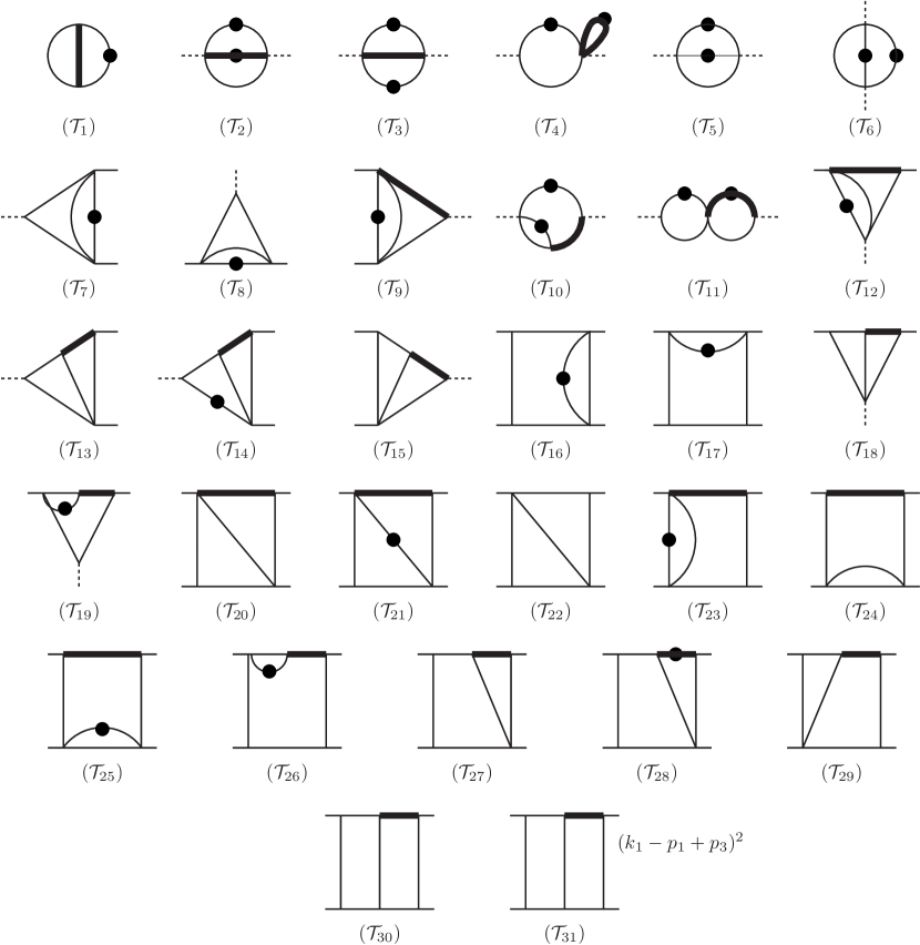
Figure 4: Two-loop one-mass MIs $\mathcal{T}_{1,\ldots,31}$. The conventions are as in figure 3.

Once again, by means of Magnus exponentials, we are able to obtain a canonical basis:

$$\text{I}_{1} =\text{F}_{1}\,, \text{I}_{2} =-s\,\text{F}_{2}\,, \text{I}_{3} =2\,m^{2}\,\text{F}_{2}+\lambda_{-}\,\text{F}_{3}\,,$$

$$\text{I}_{4} =-s\,\text{F}_{4}\,, \text{I}_{5} =-s\,\text{F}_{5}\,, \text{I}_{6} =-t\,\text{F}_{6}\,,$$

$$\text{I}_{7} =-s\,\text{F}_{7}\,, \text{I}_{8} =-t\,\text{F}_{8}\,, \text{I}_{9} =-s\,\text{F}_{9}\,,$$

$$\text{I}_{10} =\frac{m^{2}}{2\lambda_{+}}(2s\lambda_{-}\,\text{F}_{10}-2\,\text{F}_{1}-3s\,\text{F}_{5})\,, \text{I}_{11} =s^{2}\,\text{F}_{11}\,, \text{I}_{12} =-t\,\text{F}_{12}\,,$$

$$\text{I}_{13} =-s\,\text{F}_{13}\,, \text{I}_{14} =s^{2}\,\text{F}_{14}\,, \text{I}_{15} =-s\,\text{F}_{15}\,,$$

$$\text{I}_{16} =s\,t\,\text{F}_{16}\,, \text{I}_{17} =s\,t\,\text{F}_{17}\,, \text{I}_{18} =-t\,\text{F}_{18}\,,$$

$$\text{I}_{19} =-m^{2}\,t\,\text{F}_{19}\,, \text{I}_{20} =u\,\text{F}_{20}\,, \text{I}_{21} =-t\,\lambda_{-}\,\text{F}_{21}\,,$$

$$\text{I}_{22} =u\,\text{F}_{22}\,, \text{I}_{23} =-t\,\lambda_{-}\,\text{F}_{23}\,, \text{I}_{24} =-t\,\text{F}_{24}\,,$$

$$\text{I}_{25} =-t\,\lambda_{-}\,\text{F}_{25}\,, \text{I}_{26} =-t\,m^{2}\,(\text{F}_{17}+\lambda_{-}\,\text{F}_{26})\,, \text{I}_{27} =s\,t\,\text{F}_{27}\,,$$

$$\text{I}_{28} =m^{2}\,s\,\big{(}(m^{2}+t)\,\text{F}_{28}-2\,\text{F}_{27}\big{)}\,, \text{I}_{29} =(s\,t+m^{2}\,u)\,\text{F}_{29}\,, \text{I}_{30} =s\,\,t\,\lambda_{-}\text{F}_{30}\,,$$

$$\text{I}_{31} =m^{2}\,s\,\text{F}_{29}-s\,\lambda_{-}\,\text{F}_{31}\,,$$ (55)

where $\lambda_{\pm}=\left(m^{2}\pm s\right)$. After combining the two differential equations into one total differential, we find a $\operatorname{\mathit{d}log}$-form (15) with the alphabet

$$\eta_{1} =x\,, \eta_{2} =1+x\,, \eta_{3} =y\,,$$

$$\eta_{4} =1-y\,, \eta_{5} =x+y\,, \eta_{6} =x+y+xy\,,$$ (56)

which includes the additional letter $\eta_{6}$ as compared to one-loop (51). If $x>0$ and $0<y<1$ all the letters $\eta_{i}$ are positive. The coefficient matrices are given in the appendix (B.1). Since the additional letter is multilinear in $x$ and $y$, also at the two-loop order we are able to obtain the solution in terms of GPLs (see the discussion in section 3.3).

We hereby list the conditions imposed to which integrals for determining their boundary constants;

• regularity at $t\rightarrow-m^{2}$ and $u\rightarrow 0$ and imposing reality on the resulting boundary constants: $\text{I}_{2,\dots,5,7\dots 10,12,14\dots 17,19\dots 31}$ ,

• limit $s\rightarrow 0$: $\text{I}_{11,13}$ ,

• limit $t\rightarrow 0$: $\text{I}_{18}$ .

This leaves us with $\text{I}_{1,6}$, to be determined by direct integration:

$$\text{I}_{1}={} -\frac{1}{2}\frac{\Gamma(1-2\epsilon)^{2}\Gamma(1+2\epsilon)}{\Gamma(1-\epsilon)^{3}\Gamma(1+\epsilon)}\,,$$ (57)

$$\text{I}_{6}={} -\frac{y^{-2\epsilon}}{\pi}\frac{\Gamma\left(\frac{1}{2}-\epsilon\right)\Gamma\left(\frac{1}{2}+\epsilon\right)\Gamma(1-2\epsilon)}{\Gamma(1-3\epsilon)\Gamma(1+\epsilon)}\,.$$ (58)

Owing to the explicit representation in terms of GPLs, all the one-mass MIs can be computed in the whole $(s,t)$ domain (see appendix A). Our results have been successfully checked against SecDec.

The analytic expressions of all the MIs are explicitly given in electronic form in ancillary files that can be obtained from the arXiv version of this paper.

5 Two-mass Master Integrals

In this section we describe the computation of the MIs with two internal massive lines, namely topology $(c)$ of figure 1 and topologies $(c_{1})$-$(c_{2})$ of figure 2.

5.1 One-loop

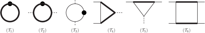
Figure 5: One-loop two-mass MIs $\mathcal{T}_{1,\ldots,6}$. The conventions are as in figure 3.

We choose the following set of MIs, admitting a differential equation linear in $\epsilon$

$$\text{F}_{1} =\epsilon\,\mathcal{T}_{1}\,, \text{F}_{2} =\epsilon\,\mathcal{T}_{2}\,, \text{F}_{3} =\epsilon\,\mathcal{T}_{3}\,,$$

$$\text{F}_{4} =\epsilon^{2}\,\mathcal{T}_{4}\,, \text{F}_{5} =\epsilon^{2}\,\mathcal{T}_{5}\,, \text{F}_{6} =\epsilon^{2}\,\mathcal{T}_{6}\,,$$ (59)

where the $\mathcal{T}_{i}$ are shown in figure 5. After applying the Magnus transformation we obtain the following canonical basis

$$\text{I}_{1} =\text{F}_{1}\,, \text{I}_{2} =-s\,\sqrt{1-\frac{4m^{2}}{s}}\,\text{F}_{2}\,, \text{I}_{3} =-t\,\text{F}_{3}\,,$$

$$\text{I}_{4} =-s\,\text{F}_{4}\,, \text{I}_{5} =-t\,\text{F}_{5}\,, \text{I}_{6} =s\,t\,\sqrt{1-4\frac{m^{2}}{s}\left(1+\frac{m^{2}}{t}\right)}\,\text{F}_{6}\,,$$ (60)

The alphabet of the corresponding canonical $\operatorname{\mathit{d}log}$-form, (15), is non-rational in $s,t$ and $m$. In particular four square roots appear

$$\sqrt{-s},\,\sqrt{4m^{2}-s},\sqrt{-t},\,\text{and}\,\,\sqrt{1-\frac{4\,m^{2}}{s}\left(1+\frac{m^{2}}{t}\right)}\,.$$ (61)

The latter can be rationalized through the change of variables

$$-\frac{s}{m^{2}}=\frac{(1-w)^{2}}{w}\,,\qquad-\frac{t}{m^{2}}=\frac{w}{z}\frac{(1+z)^{2}}{(1+w)^{2}}\,.$$ (62)

We note that the above mapping is not invertible at $s=4m^{2}$. In terms of $w$ and $z$, the alphabet reads

$$\eta_{1} =z\,, \eta_{2} =1+z\,, \eta_{3} =1-z\,,$$

$$\eta_{4} =w\,, \eta_{5} =1+w\,, \eta_{6} =1-w\,,$$

$$\eta_{7} =z-w\,, \eta_{8} =z+w^{2}\,, \eta_{9} =1-w\,z\,,$$

$$\eta_{10} =1+w^{2}\,z\,,$$ (63)

and the coefficient matrices are

$$\begin{aligned} \mathbb{M}_{1}&=\scalebox{0.6}{\mbox{$\displaystyle\left(\begin{array}[]{cccccc}\hphantom{\scalebox{0.5}[1.0]{$-$}}0&\hphantom{\scalebox{0.5}[1.0]{$-$}}0&\hphantom{\scalebox{0.5}[1.0]{$-$}}0&\hphantom{\scalebox{0.5}[1.0]{$-$}}0&\hphantom{\scalebox{0.5}[1.0]{$-$}}0&\hphantom{\scalebox{0.5}[1.0]{$-$}}0\\ \hphantom{\scalebox{0.5}[1.0]{$-$}}0&\hphantom{\scalebox{0.5}[1.0]{$-$}}0&\hphantom{\scalebox{0.5}[1.0]{$-$}}0&\hphantom{\scalebox{0.5}[1.0]{$-$}}0&\hphantom{\scalebox{0.5}[1.0]{$-$}}0&\hphantom{\scalebox{0.5}[1.0]{$-$}}0\\ \hphantom{\scalebox{0.5}[1.0]{$-$}}0&\hphantom{\scalebox{0.5}[1.0]{$-$}}0&\hphantom{\scalebox{0.5}[1.0]{$-$}}1&\hphantom{\scalebox{0.5}[1.0]{$-$}}0&\hphantom{\scalebox{0.5}[1.0]{$-$}}0&\hphantom{\scalebox{0.5}[1.0]{$-$}}0\\ \hphantom{\scalebox{0.5}[1.0]{$-$}}0&\hphantom{\scalebox{0.5}[1.0]{$-$}}0&\hphantom{\scalebox{0.5}[1.0]{$-$}}0&\hphantom{\scalebox{0.5}[1.0]{$-$}}0&\hphantom{\scalebox{0.5}[1.0]{$-$}}0&\hphantom{\scalebox{0.5}[1.0]{$-$}}0\\ \hphantom{\scalebox{0.5}[1.0]{$-$}}1&\hphantom{\scalebox{0.5}[1.0]{$-$}}0&\scalebox{0.5}[1.0]{$-$}1&\hphantom{\scalebox{0.5}[1.0]{$-$}}0&\hphantom{\scalebox{0.5}[1.0]{$-$}}0&\hphantom{\scalebox{0.5}[1.0]{$-$}}0\\ \hphantom{\scalebox{0.5}[1.0]{$-$}}0&\hphantom{\scalebox{0.5}[1.0]{$-$}}2&\hphantom{\scalebox{0.5}[1.0]{$-$}}0&\hphantom{\scalebox{0.5}[1.0]{$-$}}0&\hphantom{\scalebox{0.5}[1.0]{$-$}}0&\hphantom{\scalebox{0.5}[1.0]{$-$}}0\\ \end{array}\right)$}}\,,&\quad\mathbb{M}_{4}&=\scalebox{0.6}{\mbox{$\displaystyle\left(\begin{array}[]{cccccc}\hphantom{\scalebox{0.5}[1.0]{$-$}}0&\hphantom{\scalebox{0.5}[1.0]{$-$}}0&\hphantom{\scalebox{0.5}[1.0]{$-$}}0&\hphantom{\scalebox{0.5}[1.0]{$-$}}0&\hphantom{\scalebox{0.5}[1.0]{$-$}}0&\hphantom{\scalebox{0.5}[1.0]{$-$}}0\\ \hphantom{\scalebox{0.5}[1.0]{$-$}}1&\hphantom{\scalebox{0.5}[1.0]{$-$}}1&\hphantom{\scalebox{0.5}[1.0]{$-$}}0&\hphantom{\scalebox{0.5}[1.0]{$-$}}0&\hphantom{\scalebox{0.5}[1.0]{$-$}}0&\hphantom{\scalebox{0.5}[1.0]{$-$}}0\\ \hphantom{\scalebox{0.5}[1.0]{$-$}}0&\hphantom{\scalebox{0.5}[1.0]{$-$}}0&\scalebox{0.5}[1.0]{$-$}1&\hphantom{\scalebox{0.5}[1.0]{$-$}}0&\hphantom{\scalebox{0.5}[1.0]{$-$}}0&\hphantom{\scalebox{0.5}[1.0]{$-$}}0\\ \hphantom{\scalebox{0.5}[1.0]{$-$}}0&\scalebox{0.5}[1.0]{$-$}2&\hphantom{\scalebox{0.5}[1.0]{$-$}}0&\scalebox{0.5}[1.0]{$-$}1&\hphantom{\scalebox{0.5}[1.0]{$-$}}0&\hphantom{\scalebox{0.5}[1.0]{$-$}}0\\ \hphantom{\scalebox{0.5}[1.0]{$-$}}0&\hphantom{\scalebox{0.5}[1.0]{$-$}}0&\hphantom{\scalebox{0.5}[1.0]{$-$}}0&\hphantom{\scalebox{0.5}[1.0]{$-$}}0&\hphantom{\scalebox{0.5}[1.0]{$-$}}1&\hphantom{\scalebox{0.5}[1.0]{$-$}}0\\ \hphantom{\scalebox{0.5}[1.0]{$-$}}0&\hphantom{\scalebox{0.5}[1.0]{$-$}}0&\hphantom{\scalebox{0.5}[1.0]{$-$}}0&\hphantom{\scalebox{0.5}[1.0]{$-$}}0&\hphantom{\scalebox{0.5}[1.0]{$-$}}0&\scalebox{0.5}[1.0]{$-$}1\\ \end{array}\right)$}}\,,&\quad\mathbb{M}_{5}&=\scalebox{0.6}{\mbox{$\displaystyle\left(\begin{array}[]{cccccc}\hphantom{\scalebox{0.5}[1.0]{$-$}}0&\hphantom{\scalebox{0.5}[1.0]{$-$}}0&\hphantom{\scalebox{0.5}[1.0]{$-$}}0&\hphantom{\scalebox{0.5}[1.0]{$-$}}0&\hphantom{\scalebox{0.5}[1.0]{$-$}}0&\hphantom{\scalebox{0.5}[1.0]{$-$}}0\\ \hphantom{\scalebox{0.5}[1.0]{$-$}}0&\scalebox{0.5}[1.0]{$-$}2&\hphantom{\scalebox{0.5}[1.0]{$-$}}0&\hphantom{\scalebox{0.5}[1.0]{$-$}}0&\hphantom{\scalebox{0.5}[1.0]{$-$}}0&\hphantom{\scalebox{0.5}[1.0]{$-$}}0\\ \hphantom{\scalebox{0.5}[1.0]{$-$}}0&\hphantom{\scalebox{0.5}[1.0]{$-$}}0&\hphantom{\scalebox{0.5}[1.0]{$-$}}2&\hphantom{\scalebox{0.5}[1.0]{$-$}}0&\hphantom{\scalebox{0.5}[1.0]{$-$}}0&\hphantom{\scalebox{0.5}[1.0]{$-$}}0\\ \hphantom{\scalebox{0.5}[1.0]{$-$}}0&\hphantom{\scalebox{0.5}[1.0]{$-$}}0&\hphantom{\scalebox{0.5}[1.0]{$-$}}0&\hphantom{\scalebox{0.5}[1.0]{$-$}}0&\hphantom{\scalebox{0.5}[1.0]{$-$}}0&\hphantom{\scalebox{0.5}[1.0]{$-$}}0\\ \hphantom{\scalebox{0.5}[1.0]{$-$}}2&\hphantom{\scalebox{0.5}[1.0]{$-$}}0&\scalebox{0.5}[1.0]{$-$}2&\hphantom{\scalebox{0.5}[1.0]{$-$}}0&\hphantom{\scalebox{0.5}[1.0]{$-$}}0&\hphantom{\scalebox{0.5}[1.0]{$-$}}0\\ \hphantom{\scalebox{0.5}[1.0]{$-$}}0&\hphantom{\scalebox{0.5}[1.0]{$-$}}0&\hphantom{\scalebox{0.5}[1.0]{$-$}}0&\hphantom{\scalebox{0.5}[1.0]{$-$}}0&\hphantom{\scalebox{0.5}[1.0]{$-$}}0&\scalebox{0.5}[1.0]{$-$}2\\ \end{array}\right)$}}\,,&\quad\mathbb{M}_{7}&=\scalebox{0.6}{\mbox{$\displaystyle\left(\begin{array}[]{cccccc}\hphantom{\scalebox{0.5}[1.0]{$-$}}0&\hphantom{\scalebox{0.5}[1.0]{$-$}}0&\hphantom{\scalebox{0.5}[1.0]{$-$}}0&\hphantom{\scalebox{0.5}[1.0]{$-$}}0&\hphantom{\scalebox{0.5}[1.0]{$-$}}0&\hphantom{\scalebox{0.5}[1.0]{$-$}}0\\ \hphantom{\scalebox{0.5}[1.0]{$-$}}0&\hphantom{\scalebox{0.5}[1.0]{$-$}}0&\hphantom{\scalebox{0.5}[1.0]{$-$}}0&\hphantom{\scalebox{0.5}[1.0]{$-$}}0&\hphantom{\scalebox{0.5}[1.0]{$-$}}0&\hphantom{\scalebox{0.5}[1.0]{$-$}}0\\ \hphantom{\scalebox{0.5}[1.0]{$-$}}0&\hphantom{\scalebox{0.5}[1.0]{$-$}}0&\hphantom{\scalebox{0.5}[1.0]{$-$}}0&\hphantom{\scalebox{0.5}[1.0]{$-$}}0&\hphantom{\scalebox{0.5}[1.0]{$-$}}0&\hphantom{\scalebox{0.5}[1.0]{$-$}}0\\ \hphantom{\scalebox{0.5}[1.0]{$-$}}0&\hphantom{\scalebox{0.5}[1.0]{$-$}}0&\hphantom{\scalebox{0.5}[1.0]{$-$}}0&\hphantom{\scalebox{0.5}[1.0]{$-$}}0&\hphantom{\scalebox{0.5}[1.0]{$-$}}0&\hphantom{\scalebox{0.5}[1.0]{$-$}}0\\ \scalebox{0.5}[1.0]{$-$}1&\hphantom{\scalebox{0.5}[1.0]{$-$}}0&\hphantom{\scalebox{0.5}[1.0]{$-$}}1&\hphantom{\scalebox{0.5}[1.0]{$-$}}0&\scalebox{0.5}[1.0]{$-$}1&\hphantom{\scalebox{0.5}[1.0]{$-$}}0\\ \scalebox{0.5}[1.0]{$-$}2&\hphantom{\scalebox{0.5}[1.0]{$-$}}0&\hphantom{\scalebox{0.5}[1.0]{$-$}}2&\hphantom{\scalebox{0.5}[1.0]{$-$}}0&\scalebox{0.5}[1.0]{$-$}2&\hphantom{\scalebox{0.5}[1.0]{$-$}}0\\ \end{array}\right)$}}\,,\\ \end{aligned}$$

$$\begin{aligned} \mathbb{M}_{8}&=\scalebox{0.6}{\mbox{$\displaystyle\left(\begin{array}[]{cccccc}\hphantom{\scalebox{0.5}[1.0]{$-$}}0&\hphantom{\scalebox{0.5}[1.0]{$-$}}0&\hphantom{\scalebox{0.5}[1.0]{$-$}}0&\hphantom{\scalebox{0.5}[1.0]{$-$}}0&\hphantom{\scalebox{0.5}[1.0]{$-$}}0&\hphantom{\scalebox{0.5}[1.0]{$-$}}0\\ \hphantom{\scalebox{0.5}[1.0]{$-$}}0&\hphantom{\scalebox{0.5}[1.0]{$-$}}0&\hphantom{\scalebox{0.5}[1.0]{$-$}}0&\hphantom{\scalebox{0.5}[1.0]{$-$}}0&\hphantom{\scalebox{0.5}[1.0]{$-$}}0&\hphantom{\scalebox{0.5}[1.0]{$-$}}0\\ \hphantom{\scalebox{0.5}[1.0]{$-$}}0&\hphantom{\scalebox{0.5}[1.0]{$-$}}0&\hphantom{\scalebox{0.5}[1.0]{$-$}}0&\hphantom{\scalebox{0.5}[1.0]{$-$}}0&\hphantom{\scalebox{0.5}[1.0]{$-$}}0&\hphantom{\scalebox{0.5}[1.0]{$-$}}0\\ \hphantom{\scalebox{0.5}[1.0]{$-$}}0&\hphantom{\scalebox{0.5}[1.0]{$-$}}0&\hphantom{\scalebox{0.5}[1.0]{$-$}}0&\hphantom{\scalebox{0.5}[1.0]{$-$}}0&\hphantom{\scalebox{0.5}[1.0]{$-$}}0&\hphantom{\scalebox{0.5}[1.0]{$-$}}0\\ \hphantom{\scalebox{0.5}[1.0]{$-$}}0&\hphantom{\scalebox{0.5}[1.0]{$-$}}0&\hphantom{\scalebox{0.5}[1.0]{$-$}}0&\hphantom{\scalebox{0.5}[1.0]{$-$}}0&\hphantom{\scalebox{0.5}[1.0]{$-$}}0&\hphantom{\scalebox{0.5}[1.0]{$-$}}0\\ \hphantom{\scalebox{0.5}[1.0]{$-$}}0&\hphantom{\scalebox{0.5}[1.0]{$-$}}0&\hphantom{\scalebox{0.5}[1.0]{$-$}}0&\hphantom{\scalebox{0.5}[1.0]{$-$}}2&\hphantom{\scalebox{0.5}[1.0]{$-$}}2&\hphantom{\scalebox{0.5}[1.0]{$-$}}1\\ \end{array}\right)$}}\,,&\qquad\mathbb{M}_{9}&=\scalebox{0.6}{\mbox{$\displaystyle\left(\begin{array}[]{cccccc}\hphantom{\scalebox{0.5}[1.0]{$-$}}0&\hphantom{\scalebox{0.5}[1.0]{$-$}}0&\hphantom{\scalebox{0.5}[1.0]{$-$}}0&\hphantom{\scalebox{0.5}[1.0]{$-$}}0&\hphantom{\scalebox{0.5}[1.0]{$-$}}0&\hphantom{\scalebox{0.5}[1.0]{$-$}}0\\ \hphantom{\scalebox{0.5}[1.0]{$-$}}0&\hphantom{\scalebox{0.5}[1.0]{$-$}}0&\hphantom{\scalebox{0.5}[1.0]{$-$}}0&\hphantom{\scalebox{0.5}[1.0]{$-$}}0&\hphantom{\scalebox{0.5}[1.0]{$-$}}0&\hphantom{\scalebox{0.5}[1.0]{$-$}}0\\ \hphantom{\scalebox{0.5}[1.0]{$-$}}0&\hphantom{\scalebox{0.5}[1.0]{$-$}}0&\hphantom{\scalebox{0.5}[1.0]{$-$}}0&\hphantom{\scalebox{0.5}[1.0]{$-$}}0&\hphantom{\scalebox{0.5}[1.0]{$-$}}0&\hphantom{\scalebox{0.5}[1.0]{$-$}}0\\ \hphantom{\scalebox{0.5}[1.0]{$-$}}0&\hphantom{\scalebox{0.5}[1.0]{$-$}}0&\hphantom{\scalebox{0.5}[1.0]{$-$}}0&\hphantom{\scalebox{0.5}[1.0]{$-$}}0&\hphantom{\scalebox{0.5}[1.0]{$-$}}0&\hphantom{\scalebox{0.5}[1.0]{$-$}}0\\ \scalebox{0.5}[1.0]{$-$}1&\hphantom{\scalebox{0.5}[1.0]{$-$}}0&\hphantom{\scalebox{0.5}[1.0]{$-$}}1&\hphantom{\scalebox{0.5}[1.0]{$-$}}0&\scalebox{0.5}[1.0]{$-$}1&\hphantom{\scalebox{0.5}[1.0]{$-$}}0\\ \hphantom{\scalebox{0.5}[1.0]{$-$}}2&\hphantom{\scalebox{0.5}[1.0]{$-$}}0&\scalebox{0.5}[1.0]{$-$}2&\hphantom{\scalebox{0.5}[1.0]{$-$}}0&\hphantom{\scalebox{0.5}[1.0]{$-$}}2&\hphantom{\scalebox{0.5}[1.0]{$-$}}0\\ \end{array}\right)$}}\,,&\qquad\mathbb{M}_{10}&=\scalebox{0.6}{\mbox{$\displaystyle\left(\begin{array}[]{cccccc}\hphantom{\scalebox{0.5}[1.0]{$-$}}0&\hphantom{\scalebox{0.5}[1.0]{$-$}}0&\hphantom{\scalebox{0.5}[1.0]{$-$}}0&\hphantom{\scalebox{0.5}[1.0]{$-$}}0&\hphantom{\scalebox{0.5}[1.0]{$-$}}0&\hphantom{\scalebox{0.5}[1.0]{$-$}}0\\ \hphantom{\scalebox{0.5}[1.0]{$-$}}0&\hphantom{\scalebox{0.5}[1.0]{$-$}}0&\hphantom{\scalebox{0.5}[1.0]{$-$}}0&\hphantom{\scalebox{0.5}[1.0]{$-$}}0&\hphantom{\scalebox{0.5}[1.0]{$-$}}0&\hphantom{\scalebox{0.5}[1.0]{$-$}}0\\ \hphantom{\scalebox{0.5}[1.0]{$-$}}0&\hphantom{\scalebox{0.5}[1.0]{$-$}}0&\hphantom{\scalebox{0.5}[1.0]{$-$}}0&\hphantom{\scalebox{0.5}[1.0]{$-$}}0&\hphantom{\scalebox{0.5}[1.0]{$-$}}0&\hphantom{\scalebox{0.5}[1.0]{$-$}}0\\ \hphantom{\scalebox{0.5}[1.0]{$-$}}0&\hphantom{\scalebox{0.5}[1.0]{$-$}}0&\hphantom{\scalebox{0.5}[1.0]{$-$}}0&\hphantom{\scalebox{0.5}[1.0]{$-$}}0&\hphantom{\scalebox{0.5}[1.0]{$-$}}0&\hphantom{\scalebox{0.5}[1.0]{$-$}}0\\ \hphantom{\scalebox{0.5}[1.0]{$-$}}0&\hphantom{\scalebox{0.5}[1.0]{$-$}}0&\hphantom{\scalebox{0.5}[1.0]{$-$}}0&\hphantom{\scalebox{0.5}[1.0]{$-$}}0&\hphantom{\scalebox{0.5}[1.0]{$-$}}0&\hphantom{\scalebox{0.5}[1.0]{$-$}}0\\ \hphantom{\scalebox{0.5}[1.0]{$-$}}0&\hphantom{\scalebox{0.5}[1.0]{$-$}}0&\hphantom{\scalebox{0.5}[1.0]{$-$}}0&\scalebox{0.5}[1.0]{$-$}2&\scalebox{0.5}[1.0]{$-$}2&\hphantom{\scalebox{0.5}[1.0]{$-$}}1\\ \end{array}\right)$}}\,,\end{aligned}$$ (64)

and $(\mathbb{M}_{2})_{3,3}=-2$ and $(\mathbb{M}_{2})_{5,5}=2$ are the only non-vanishing entries in $\mathbb{M}_{2}$, $(\mathbb{M}_{3})_{6,6}=-2$ is the only non-vanishing entry in $\mathbb{M}_{3}$, and $(\mathbb{M}_{6})_{4,4}=2$ is the only non-vanishing entry in $\mathbb{M}_{6}$. In the region $0<w<z<1$ all the letters $\eta_{i}$ are positive. For a detailed discussion of how the interesting regions in the $s,t$ plane are mapped to the $\mathbb{C}\times\mathbb{C}$ space of the $w,z$ variables, see appendix A. The alphabet in (63) is linear in $z$ but contains letters quadratic in $w$. As the latter can be linearized by factorization over the complex numbers, we are once again able to express the solution in terms of GPLs (see the discussion in section 3.3).

The integration constants of $\text{I}_{4,5,6}$ can be fixed by requiring their regularity at the pseudothresholds $s\rightarrow 0$, $t\rightarrow-m^{2}$ and $u\rightarrow 0$. The boundary constant of $\text{I}_{2}$ can be fixed by taking the $s\rightarrow 0$ limit. This leaves us with two integrals, $\text{I}_{1,3}$, to be determined by direct integration:

$$\text{I}_{1}={} \frac{\Gamma(1-2\epsilon)}{\Gamma(1-\epsilon)^{2}}\,,$$ (65)

$$\text{I}_{3}={} \left[\frac{z}{w}\frac{(1+w)^{2}}{(1+z)^{2}}\right]^{\epsilon}\,.$$ (66)

5.2 Two-loop

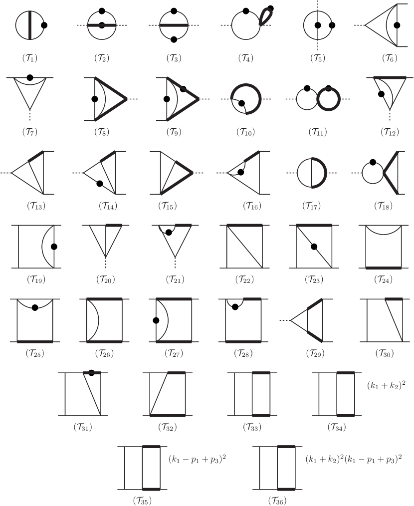
Figure 6: Two-loop two-mass MIs $\mathcal{T}_{1,\ldots,36}$. The conventions are as in figure 3.

At the two-loop order we start with the set of MIs

$$\text{F}_{1} =(1-\epsilon)\,\epsilon^{2}\,\mathcal{T}_{1}\,, \text{F}_{2} =\epsilon^{2}\,\mathcal{T}_{2}\,, \text{F}_{3} =\epsilon^{2}\,\mathcal{T}_{3}\,,$$

$$\text{F}_{4} =\epsilon^{2}\,\mathcal{T}_{4}\,, \text{F}_{5} =\epsilon^{2}\,\mathcal{T}_{5}\,, \text{F}_{6} =\epsilon^{3}\,\mathcal{T}_{6}\,,$$

$$\text{F}_{7} =\epsilon^{3}\,\mathcal{T}_{7}\,, \text{F}_{8} =\epsilon^{3}\,\mathcal{T}_{8}\,, \text{F}_{9} =\epsilon^{2}\,\mathcal{T}_{9}\,,$$

$$\text{F}_{10} =(1-2\epsilon)\,\epsilon^{2}\,\mathcal{T}_{10}\,, \text{F}_{11} =\epsilon^{2}\,\mathcal{T}_{11}\,, \text{F}_{12} =\epsilon^{3}\,\mathcal{T}_{12}\,,$$

$$\text{F}_{13} =\epsilon^{4}\,\mathcal{T}_{13}\,, \text{F}_{14} =\epsilon^{3}\,\mathcal{T}_{14}\,, \text{F}_{15} =\epsilon^{4}\,\mathcal{T}_{15}\,,$$

$$\text{F}_{16} =\epsilon^{3}\,\mathcal{T}_{16}\,, \text{F}_{17} =(1-2\epsilon)\,\epsilon^{3}\,\mathcal{T}_{17}\,, \text{F}_{18} =\epsilon^{3}\,\mathcal{T}_{18}\,,$$

$$\text{F}_{19} =\epsilon^{3}\,\mathcal{T}_{19}\,, \text{F}_{20} =\epsilon^{4}\,\mathcal{T}_{20}\,, \text{F}_{21} =\epsilon^{3}\,\mathcal{T}_{21}\,,$$

$$\text{F}_{22} =\epsilon^{4}\,\mathcal{T}_{22}\,, \text{F}_{23} =\epsilon^{3}\,\mathcal{T}_{23}\,, \text{F}_{24} =(1-2\epsilon)\epsilon^{3}\,\mathcal{T}_{24}\,,$$

$$\text{F}_{25} =\epsilon^{3}\,\mathcal{T}_{25}\,, \text{F}_{26} =(1-2\epsilon)\,\epsilon^{3}\,\mathcal{T}_{26}\,, \text{F}_{27} =\epsilon^{3}\,\mathcal{T}_{27}\,,$$

$$\text{F}_{28} =\epsilon^{3}\,\mathcal{T}_{28}\,, \text{F}_{29} =\epsilon^{4}\,\mathcal{T}_{29}\,, \text{F}_{30} =\epsilon^{4}\,\mathcal{T}_{30}\,,$$

$$\text{F}_{31} =\epsilon^{3}\,\mathcal{T}_{31}\,, \text{F}_{32} =\epsilon^{4}\,\mathcal{T}_{32}\,, \text{F}_{33} =\epsilon^{4}\,\mathcal{T}_{33}\,,$$

$$\text{F}_{34} =\epsilon^{4}\,\mathcal{T}_{34}\,, \text{F}_{35} =\epsilon^{4}\,\mathcal{T}_{35}\,, \text{F}_{36} =\epsilon^{4}\,\mathcal{T}_{36}\,,$$ (67)

where the $\mathcal{T}_{i}$ are shown in figure 6. The MIs $\mathbf{F}$ admit $\epsilon$-linear differential equations, except for one of them. We have indeed

$$d\mathbf{F}=d\mathbb{K}\,\mathbf{F},\qquad\mathbb{K}=\mathbb{K}_{0}+\epsilon\,\mathbb{K}_{1}+\frac{1}{1-2\epsilon}\mathbb{K}_{2}\,,$$ (68)

where $\mathbb{K}_{0},\mathbb{K}_{1}$ and $\mathbb{K}_{2}$ do not depend on $\epsilon$, and $\mathbb{K}_{2}$ is non-vanishing only in the inhomogeneous part of the differential equation for $\text{F}_{36}$. In a first step we apply the Magnus algorithm on $\mathbb{K}_{0}+\epsilon\,\mathbb{K}_{1}$ in order to remove $\mathbb{K}_{0}$, and in a second step we apply an ad-hoc transformation in order to remove the remaining non-linear piece.

The corresponding canonical basis reads

$$\begin{aligned} \text{I}_{1}&=\text{F}_{1}\,,&\qquad\text{I}_{2}&=-s\,\text{F}_{2}\,,&\qquad\text{I}_{3}&=m^{2}\,(2\,\text{F}_{2}+\text{F}_{3})-s\,\text{F}_{3}\,,&\qquad\text{I}_{4}&=-s\,\text{F}_{4}\,,\\ \text{I}_{5}&=-t\,\text{F}_{5}\,,&\text{I}_{6}&=-s\,\text{F}_{6}\,,&\text{I}_{7}&=-t\,\text{F}_{7}\,,&\text{I}_{8}&=-s\,\text{F}_{8}\,,\end{aligned}$$

$$\begin{aligned} \text{I}_{9}&=-\sqrt{1-\frac{4\,m^{2}}{s}}\left(\frac{3}{2}\,\text{F}_{8}+m^{2}\,\text{F}_{9}\right)-\frac{3}{2}s\,\text{F}_{8}\,,\\ \end{aligned}$$

$$\begin{aligned} \text{I}_{10}={}&\frac{1}{4}\left(1+\sqrt{\frac{-s}{4m^{2}-s}}\right)\left(-2\text{F}_{1}+(\,m^{2}-s)\,\left(\text{F}_{2}+\text{F}_{3}\right)+m^{2}\,\text{F}_{2}\phantom{\sqrt{1-\frac{4\,m^{2}}{s}}}\right.\\ &\qquad\qquad\qquad\qquad\qquad\left.+s\,\text{F}_{10}-s\,\sqrt{1-\frac{4\,m^{2}}{s}}\left(\text{F}_{2}+\text{F}_{10}\right)\right)\,,\end{aligned}$$

$$\begin{aligned} \text{I}_{11}&=s^{2}\,\sqrt{1-\frac{4\,m^{2}}{s}}\,\text{F}_{11}\,,&\qquad\text{I}_{12}&=-t\,\text{F}_{12}\,,&\qquad\text{I}_{13}&=-s\,\text{F}_{13}\,,\\ \text{I}_{14}&=s^{2}\,\text{F}_{14}\,,&\text{I}_{15}&=-s\,\text{F}_{15}\,,&\text{I}_{16}&=-m^{2}\,s\,\text{F}_{16}\,,\\ \text{I}_{17}&=-s\,\text{F}_{17}\,,&\text{I}_{18}&=s^{2}\,\text{F}_{18}\,,&\text{I}_{19}&=s\,t\,\text{F}_{19}\,,\\ \text{I}_{20}&=-t\,\text{F}_{20}\,,&\text{I}_{21}&=-m^{2}\,t\,\text{F}_{21}\,,&\text{I}_{22}&=u\,\text{F}_{22}\,,\\ \text{I}_{23}&=(s-m^{2})\,t\,\text{F}_{23}\,,&\text{I}_{24}&=-t\,\text{F}_{24}\,,&\text{I}_{25}&=(s-m^{2})\,t\,\text{F}_{25}\,,\\ \end{aligned}$$

$$\begin{aligned} \text{I}_{26}&=-s\,\text{F}_{26}\,,&\qquad\text{I}_{27}&=s\,t\,\sqrt{1-\frac{4\,m^{2}}{s}\left(1+\frac{m^{2}}{t}\right)}\,\text{F}_{27}\,,\\ \end{aligned}$$

$$\begin{aligned} \text{I}_{28}&=s\,t\,\sqrt{1-\frac{4\,m^{2}}{s}\left(1+\frac{m^{2}}{t}\right)}(\text{F}_{25}+m^{2}\text{F}_{28})+t\,(m^{2}-s)\,\text{F}_{25}\,,\end{aligned}$$

$$\begin{aligned} \text{I}_{29}&=s^{2}\,\sqrt{1-\frac{4\,m^{2}}{s}}\,\text{F}_{29}\,,&\qquad\text{I}_{30}&=s\,t\,\text{F}_{30}\,,\\ \text{I}_{31}&=-m^{2}\,s\,(2\text{F}_{30}+(m^{2}+t)\,\text{F}_{31})\,,&\text{I}_{32}&=s\,t\,\sqrt{1+\frac{m^{4}}{t^{2}}-\frac{2\,m^{2}}{s}\left(1-\frac{u}{t}\right)}\,\text{F}_{32}\,,\\ \text{I}_{33}&=-s^{2}\,t\,\sqrt{1-\frac{4\,m^{2}}{s}\left(1+\frac{m^{2}}{t}\right)}\,\text{F}_{33}\,,&\text{I}_{34}&=s^{2}\,\text{F}_{34}\,,\end{aligned}$$

$$\begin{aligned} \text{I}_{35}={}&s\,\sqrt{1-\frac{4\,m^{2}}{s}}\left(2\,t\,\text{F}_{32}-s\,t\,\text{F}_{33}+s\,\text{F}_{35}\right)-s^{2}\,t\,\sqrt{1+\frac{4\,m^{2}}{s}\left(1+\frac{m^{2}}{t}\right)}\,\text{F}_{33}\,,\\ \end{aligned}$$

$$\begin{aligned} \text{I}_{36}={}&\frac{s}{2(1-2\epsilon)}\,\text{F}_{17}-s\,t\,\left(1-\sqrt{1-\frac{4\,m^{2}}{s}}\right)\text{F}_{32}-s\,t\,\text{F}_{18}-2\,t\text{F}_{22}\\ &-\frac{2m^{2}\,s}{2-\frac{s}{m^{2}}\,(1-\sqrt{1-\frac{4m^{2}}{s}})}\,(\text{F}_{29}+t\,\text{F}_{33}-\text{F}_{35})-s\,\text{F}_{36}\,.\end{aligned}$$ (69)

As compared to the one-loop case (61) we encounter one additional square root in the canonical $\operatorname{\mathit{d}log}$-form

$$\sqrt{1+\frac{m^{4}}{t^{2}}-\frac{2\,m^{2}}{s}\left(1-\frac{u}{t}\right)},$$ (70)

which is not rationalized by the change of variables in eq. (62). In terms of $w$ and $z$, the alphabet reads

$$\begin{aligned} \eta_{1}&=z,&\qquad\eta_{2}&=1+z,&\qquad\eta_{3}&=1-z,\\ \eta_{4}&=w,&\eta_{5}&=1+w,&\eta_{6}&=1-w,\\ \eta_{7}&=1-w+w^{2},&\eta_{8}&=1-w\,z,&\eta_{9}&=z-w,\\ \end{aligned}$$

$$\begin{aligned} \eta_{10}&=1+w^{2}\,z,&\qquad\eta_{11}&=z+w^{2},&\end{aligned}$$

$$\begin{aligned} \eta_{12}&=4(1+z)^{4}w^{3}+(1-w)^{2}\,\kappa^{2}_{+}(w,z)\,,&\qquad\eta_{13}&=(1+w)\sqrt{\rho}+(1-w)\,\kappa_{-}(w,z)\,,\\ \eta_{14}&=(1+w)\sqrt{\rho}-(1-w)\,\kappa_{-}(w,z)\,,&\qquad\eta_{15}&=(1+w)\sqrt{\rho}+(1-w)\,\kappa_{+}(w,z)\,,\\ \end{aligned}$$

$$\begin{aligned} \eta_{16}&=\frac{c_{1}+c_{2}\,\sqrt{\rho}}{c_{3}+c_{4}\,\sqrt{\rho}}\,,\\ \end{aligned}$$

$$\begin{aligned} \eta_{17}&=2(1-w)^{2}wz^{2}+\kappa_{-}^{2}(-w,z)+\left(z+w\right)\left(1+wz\right)\sqrt{\rho}\,,\end{aligned}$$ (71)

where

$$\kappa_{\pm}(a,b)\equiv a\,(1+b)^{2}\pm b\,(1+a)^{2}\,,$$ (72)

the argument of the square root entering $\eta_{13,\ldots,17}$ is

$$\rho={} 4wz^{2}(1+w)^{2}-\kappa_{+}(w,z)\,\kappa_{+}(-w,-z)\,,$$ (73)

and the four coefficients in $\eta_{16}$ are given by

$$c_{1}={} (1+w)^{2}\left(1-4w+w^{2}\right)z^{2}(1+z)^{2}$$

$$+w^{2}(1+z)^{6}+2w\left(1-w+w^{2}\right)z(1+z)^{4}-2(1+w)^{4}z^{3}\,,$$ (74)

$$c_{2}={} \left(1-z^{2}\right)\kappa_{+}(w,z)\,,$$ (75)

$$c_{3}={} 2w^{8}z^{4}+2w^{7}z^{3}\left(z^{2}+6z+1\right)-w^{6}(z-1)^{2}z^{2}\left(z^{2}+4z+1\right)$$

$$-2w^{5}z\left(z^{6}-z^{5}-8z^{4}-8z^{3}-8z^{2}-z+1\right)$$

$$+w^{4}\left(z^{8}-2z^{7}-2z^{6}+6z^{5}-10z^{4}+6z^{3}-2z^{2}-2z+1\right)$$

$$-2w^{3}z\left(z^{6}-z^{5}-8z^{4}-8z^{3}-8z^{2}-z+1\right)$$

$$-w^{2}(z-1)^{2}z^{2}\left(z^{2}+4z+1\right)+2wz^{3}\left(z^{2}+6z+1\right)+2z^{4}\,,$$ (76)

$$c_{4}={} -w(1-z^{2})(z-w)(1-wz)\left(\kappa_{-}(-w,-z)+\left(1+w\right)^{2}z\right)\,.$$ (77)

In the region $0<w<z<1$ all the letters $\eta_{i}$ are positive.

As already stressed, the alphabet is not rational in $w$ and $z$. This prevents us from expressing the complete solution in terms of GPLs. In particular, the structure of the coefficient matrices $\mathbb{M}_{i}$ is such that the solution for $\text{I}_{32}^{(3)}$ and for $\text{I}_{32,\ldots,36}^{(4)}$, see eqs. (24), (25), involves path integration over $\operatorname{\mathit{d}log}$’s with non rational arguments. Nevertheless, the MIs $\text{I}_{1,\dots,31}$ admit a representation in terms of GPLs which is convenient for their numerical evaluation. As for the remaining MIs, we followed the procedure outlined in section 3.3: we express the solution up to weight 2 for $\text{I}_{32}$ and up to weight 3 for $\text{I}_{33,\ldots,36}$ in terms of GPLs and then obtain an 1-fold integral representation for the higher weights (for $\text{I}_{32,\dots,36}^{(4)}$ we use eq. (40)).

We hereby list the conditions imposed to integrals $\text{I}_{1,\ldots,31}$ for determining their boundary constants;

• independent input: $\text{I}_{1,4,\dots,7,13,14,20,25}$ ,

• regularity at $s\rightarrow 0$: $\text{I}_{24}$ ,

• regularity at $t\rightarrow-m^{2}$: $\text{I}_{12,21}$ ,

• regularity at $u\rightarrow 0$: $\text{I}_{19,30,31}$ ,

• limit $s\rightarrow 0$: $\text{I}_{2,3,6,\dots,10,15\dots 18,29}$ ,

• limit $t\rightarrow-m^{2}$ and $s\rightarrow 0$: $\text{I}_{28}$ ,

• regularity at $s\rightarrow 0$ and matching to independent input: $\text{I}_{22,23}$ .

For the MIs $\text{I}_{32,\ldots,36}$ we observe that regularity at $u=s=t=0$, corresponding to $\vec{x}_{0}=(w_{0},z_{0})=(1,-1)$, implies

$$\text{I}_{32,\dots,36}(\epsilon,\vec{x}_{0})=0\,,$$ (78)

that we choose as initial condition of our solution in terms of iterated integrals.

The MIs $\text{I}_{1,\ldots,31}$ are represented in terms of GPLs, and can be computed on the whole $(s,t)$ plane (except for the line $s=4m^{2}$, see appendix A for further comments).

The explicit evaluation of $\text{I}_{32,\ldots,36}$ requires a careful choice of the integration path, in such a way that no branch cuts are crossed. We successfully checked our results in the unphysical region $s<0$ (see appendix A) against the numerical values obtained with SecDec. The evaluation of our analytic result relies on the use of GiNaC for the computation of the GPLs and on a one-dimensional integration for the cases where non-rational weights appear in the most external iteration, according to the eq. (40). As for the latter, we exploited the propriety of path-independence to choose simple paths (that avoid the singularities on the way from the basepoint to the chosen endpoints). Let us remark that in this work we did not focus on the the computing performances of the numerical evaluation of the mixed Chen-Goncharov iterated integrals appearing in our analytic expression. This aspect, together with a study of the analytic properties of our solutions in the whole phase-space, requires a dedicated future investigation.

The analytic expressions of all the MIs are explicitly given in electronic form in ancillary files that can be obtained from the arXiv version of this paper.

6 Conclusions

In this article, we presented the calculation of the master integrals (MIs) needed for the virtual QCD$\times$EW two-loop corrections to the Drell-Yan scattering processes,

$$q+\bar{q}\to l^{-}+l^{+}\,\ ,\qquad q+\bar{q}^{\prime}\to l^{-}+\overline{\nu}\,,$$

for massless external particles. Besides the exchange of massless gauge bosons, such as gluons and photons, the relevant Feynman diagrams involve also the presence of $W$ and $Z$ propagators. Given the small difference between the masses of the $W$ and $Z$ bosons, in the diagrams containing both virtual particles at the same time, we performed a series expansion in the difference of the squared masses. Owing to this approximation, we distinguished three types of diagrams, according to the presence of massive internal lines: the no-mass type, the one-mass type, and the two-mass type, where all massive propagators, when occurring, contain the same mass value. The evaluations of the four point functions with one and two internal massive propagators are the main novel results of this communication.

To achieve it, we identified a basis of 49 MIs and evaluated them with the method of the differential equations. With the help of the Magnus exponential, the MIs were found to obey a canonical system of differential equations. Boundary conditions were imposed either by matching the solutions onto simpler integrals in special kinematic configurations, or by requiring the regularity of the solution at pseudo-thresholds. The canonical MIs were given as Taylor series around $d=4$ space-time dimensions, up to order four, whose coefficients were given in terms of iterated integrals up to weight four. The solution could be expressed in terms of Chen’s iterated integrals, yet, we adopted a mixed representation in terms of Chen-Goncharov iterated integrals, suitable for their numerical evaluation. Further studies concerning the analytic properties of the presented MIs in the whole phase-space, and the optimization of their numerical evaluation will be the subject of a forthcoming publication.

Appendix A Variables for the one-mass and two-mass integrals

In this section we discuss the domain of the variables employed in the analytic expressions of the MIs for the Drell-Yan process, both in the case with one massive propagator and in the one with two massive propagators.

A.1 One-mass type

For the evaluation of the one-mass MIs we simply rescale by the squared mass the Mandelstam invariants. All the analytic results are given in terms of two-dimensional generalized polylogarithms, functions of the variables

$$x=-\frac{s}{m^{2}}\,,\quad y=-\frac{t}{m^{2}}\,.$$ (79)

In the unphysical region $s<0$, $x$ is real and positive. Correspondingly, $y$ can be either positive or negative.

The analytic continuation to the physical region requires the Feynman prescription on the invariants. There, $s$ becomes positive, with a positive vanishing imaginary part, $s+i0^{+}$. Accordingly, $x$ is negative:

$$x\to-x^{\prime}-i0^{+}\,,$$ (80)

with

$$x^{\prime}=\frac{s}{m^{2}}>0\,.$$ (81)

On the other hand, $t$ is negative (with a positive vanishing imaginary part) and ranges between 0 and $-s$, $-s<t<0$.

The numeric evaluation of the MIs expressed in terms of GPLs of the variables $x$ and $y$ can be done in the whole $s,t$ plain using the routines in Vollinga:2004sn expressing our analytic formulas in terms of GPLs evaluated in 1 and giving the explicit imaginary part to the Mandelstam variables (see for instance Bonciani:2010ms ).

A.2 Two-mass type

For the evaluation of the two-mass MIs, see section 5, we find it convenient to introduce the reduced variables $w$ and $z$ defined by

$$-\frac{s}{m^{2}}=\frac{(1-w)^{2}}{w}\,,\qquad-\frac{t}{m^{2}}=\frac{w}{z}\frac{(1+z)^{2}}{(1+w)^{2}}\,.$$ (82)

We note that the above mapping allows the evaluation of our results everywhere in the $(s,t)$ plane, with the exception of the value $w=-1$ (corresponding to $s=4m^{2})$. For that specific value of $w$, the $t$ dependence in $z$ gets lost by construction, and $z=-1$ independently on $t$.

The evaluation of the solution at $s=4m^{2}$ requires further investigations and it will be addressed in a forthcoming publication.

A.2.1 Range of values for $w$

For $w$, defined by the first of eqs. (82), we choose the following root:

$$w=\frac{\sqrt{4m^{2}-s-i0^{+}}-\sqrt{-s-i0^{+}}}{\sqrt{4m^{2}-s-i0^{+}}+\sqrt{-s-i0^{+}}}\,,$$ (83)

where we explicitly used the Feynman prescription $s+i0^{+}$.

1. If $s<0$, we have positive $w$ and $0<w<1$. In particular, when $s\to-\infty$, $w\to 0$, while for $s\to 0$, $w\to 1$.

2. If $0<s<4m^{2}$, $w$ becomes a phase. In fact

   $$w=\frac{\sqrt{4m^{2}-s}+i\sqrt{s}}{\sqrt{4m^{2}-s}-i\sqrt{s}}=e^{i\phi}\,,$$ (84)

   where

   $$\phi=2\arctan{\sqrt{\frac{s}{4m^{2}-s}}}$$ (85)

   and $0<\phi<\pi$.

3. If $s>4m^{2}$, $w$ becomes negative (with a positive vanishing imaginary part)

   $$w=-\frac{\sqrt{s}-\sqrt{s-4m^{2}}}{\sqrt{s}+\sqrt{s-4m^{2}}}=-w^{\prime}+i0^{+}\,,$$ (86)

   and $1>w^{\prime}>0$ when $4m^{2}<s<+\infty$.

A.2.2 Range of values for $z$

The variable $z$ depends both on $s$ and $t$. In order to study the different regimes, we define the following function of $s$

$$t_{*}\equiv{} -m^{2}\frac{w}{(1+w)^{2}}$$

$$={} -\frac{m^{4}}{4m^{2}-s}\,.$$ (87)

where the second equality follows from eq. (83). We also define the ratio

$$K\equiv{} \frac{t}{t_{*}}\,,$$ (88)

so that the second of eqs. (82) reads

$$K=\frac{(1+z)^{2}}{z}\,.$$ (89)

We choose the following root of the above equation

$$z={} \frac{\sqrt{K}-\sqrt{K-4}}{\sqrt{K}+\sqrt{K-4}}\,.$$ (90)

Note that eq. (90) contains square-roots of $K$. Therefore, in order to compute $z$ when $K<4$, we have to keep track of the vanishing imaginary parts of the quantities entering eq. (88). Region by region in the $(s,t)$ plane, the correct sign of the vanishing imaginary part (if present) is determined by the Feynman prescription on $s,t,u$, i.e. $s+i0^{+}$ when $s>0$, and likewise for $t$ and $u$.

Depending on the value of $K$, we distinguish three cases (here we keep the prescription for the vanishing imaginary part of $K$ arbitrary):

1. $K>4$

   All the square roots in eq. (90) are real, so $z$ is real with $0<z<1$.

2. $0<K<4$

   For a given prescription $K\pm i0^{+}$, one obtains from eq. (90)

   $$z=\frac{\sqrt{K}\mp i\sqrt{4-K}}{\sqrt{K}\pm i\sqrt{4-K}}\,,$$ (91)

   which is solved by

   $$z=e^{\mp i\psi}\,,\qquad\psi=2\arctan{\sqrt{\frac{4-K}{K}}}\,,\qquad 0<\psi<\pi\,.$$ (92)

3. $K<0$

   For a given prescription $K\pm i0^{+}$, one obtains from eq. (90)

   $$z={} \frac{\sqrt{-|K|\pm i0^{+}}-\sqrt{-|K|-4\pm i0^{+}}}{{\sqrt{-|K|\pm i0^{+}}+\sqrt{-|K|-4\pm i0^{+}}}}$$

   $$={} \frac{\sqrt{|K|}-\sqrt{|K|+4}}{\sqrt{|K|}+\sqrt{|K|+4}}\mp i0^{+}$$

   $$\equiv{} -z^{\prime}\mp i0^{+}\,,$$ (93)

   with $0<z^{\prime}<1$.

Note that, since $K$ is a function of $s$ and $t$, each case can arise from multiple regions in the $(s,t)$ plane. In table 1 we summarize the solution for $z$ in the different regions of the $(s,t)$ plane, by displaying also the appropriate sign for the $i0^{+}$ prescription (if a vanishing imaginary part is present).

	$t<-4|t_{*}|$	$-4|t_{*}|<t<0$	$0<t<|t_{*}|$	$|t_{*}|<t<4|t_{*}|$	$t>|4t_{*}|$
$s<0$	$z$	$e^{-i\psi}$	$-z^{\prime}+i0^{+}$	$-z^{\prime}+i0^{+}$	$-z^{\prime}+i0^{+}$
$0<s<4m^{2}$	$z$	$\boldsymbol{e^{i\psi}}$	$-z^{\prime}+i0^{+}$	$-z^{\prime}-i0^{+}$	$-z^{\prime}-i0^{+}$
$s>4m^{2}$	$\boldsymbol{-z^{\prime}+i0^{+}}$	$\boldsymbol{-z^{\prime}+i0^{+}}$	$e^{-i\psi}$	$e^{-i\psi}$	$z$

Table 1: We show the solution for $z$ in each region of the $(s,t)$ plane, as in eqs. (90), (92), and (3). The boldface entries are the solutions in the regions that contain a part of the physical $s$-channel scattering region, $s>0$ with $-s<t<0$.

Appendix B Two-Loop $\operatorname{\mathit{d}log}$-forms

In this appendix we give explicitly the coefficient matrices of the $\operatorname{\mathit{d}log}$-forms, eq. (15), for the one-mass and the two-mass two-loop MIs, discussed respectively in sections 4 and 5.

B.1 One-mass

For the one-mass case at the two-loop order, the $\operatorname{\mathit{d}log}$-form is

$$d\mathbb{A}={} \mathbb{M}_{1}\,\operatorname{\mathit{d}log}(1+x)+\mathbb{M}_{2}\,\operatorname{\mathit{d}log}(x)+\mathbb{M}_{3}\,\operatorname{\mathit{d}log}(y)$$

$$+\mathbb{M}_{4}\,\operatorname{\mathit{d}log}(1-y)+\mathbb{M}_{5}\,\operatorname{\mathit{d}log}(x+y)+\mathbb{M}_{6}\,\operatorname{\mathit{d}log}(x+y+xy)$$ (94)

with

$$\mathbb{M}_{1}=\scalebox{0.55}{\mbox{$\displaystyle\left(\begin{array}[]{ccccccccccccccccccccccccccccccc}\hphantom{\scalebox{0.5}[1.0]{$-$}}0&\hphantom{\scalebox{0.5}[1.0]{$-$}}0&\hphantom{\scalebox{0.5}[1.0]{$-$}}0&\hphantom{\scalebox{0.5}[1.0]{$-$}}0&\hphantom{\scalebox{0.5}[1.0]{$-$}}0&\hphantom{\scalebox{0.5}[1.0]{$-$}}0&\hphantom{\scalebox{0.5}[1.0]{$-$}}0&\hphantom{\scalebox{0.5}[1.0]{$-$}}0&\hphantom{\scalebox{0.5}[1.0]{$-$}}0&\hphantom{\scalebox{0.5}[1.0]{$-$}}0&\hphantom{\scalebox{0.5}[1.0]{$-$}}0&\hphantom{\scalebox{0.5}[1.0]{$-$}}0&\hphantom{\scalebox{0.5}[1.0]{$-$}}0&\hphantom{\scalebox{0.5}[1.0]{$-$}}0&\hphantom{\scalebox{0.5}[1.0]{$-$}}0&\hphantom{\scalebox{0.5}[1.0]{$-$}}0&\hphantom{\scalebox{0.5}[1.0]{$-$}}0&\hphantom{\scalebox{0.5}[1.0]{$-$}}0&\hphantom{\scalebox{0.5}[1.0]{$-$}}0&\hphantom{\scalebox{0.5}[1.0]{$-$}}0&\hphantom{\scalebox{0.5}[1.0]{$-$}}0&\hphantom{\scalebox{0.5}[1.0]{$-$}}0&\hphantom{\scalebox{0.5}[1.0]{$-$}}0&\hphantom{\scalebox{0.5}[1.0]{$-$}}0&\hphantom{\scalebox{0.5}[1.0]{$-$}}0&\hphantom{\scalebox{0.5}[1.0]{$-$}}0&\hphantom{\scalebox{0.5}[1.0]{$-$}}0&\hphantom{\scalebox{0.5}[1.0]{$-$}}0&\hphantom{\scalebox{0.5}[1.0]{$-$}}0&\hphantom{\scalebox{0.5}[1.0]{$-$}}0&\hphantom{\scalebox{0.5}[1.0]{$-$}}0\\ \hphantom{\scalebox{0.5}[1.0]{$-$}}0&\hphantom{\scalebox{0.5}[1.0]{$-$}}1&\hphantom{\scalebox{0.5}[1.0]{$-$}}0&\hphantom{\scalebox{0.5}[1.0]{$-$}}0&\hphantom{\scalebox{0.5}[1.0]{$-$}}0&\hphantom{\scalebox{0.5}[1.0]{$-$}}0&\hphantom{\scalebox{0.5}[1.0]{$-$}}0&\hphantom{\scalebox{0.5}[1.0]{$-$}}0&\hphantom{\scalebox{0.5}[1.0]{$-$}}0&\hphantom{\scalebox{0.5}[1.0]{$-$}}0&\hphantom{\scalebox{0.5}[1.0]{$-$}}0&\hphantom{\scalebox{0.5}[1.0]{$-$}}0&\hphantom{\scalebox{0.5}[1.0]{$-$}}0&\hphantom{\scalebox{0.5}[1.0]{$-$}}0&\hphantom{\scalebox{0.5}[1.0]{$-$}}0&\hphantom{\scalebox{0.5}[1.0]{$-$}}0&\hphantom{\scalebox{0.5}[1.0]{$-$}}0&\hphantom{\scalebox{0.5}[1.0]{$-$}}0&\hphantom{\scalebox{0.5}[1.0]{$-$}}0&\hphantom{\scalebox{0.5}[1.0]{$-$}}0&\hphantom{\scalebox{0.5}[1.0]{$-$}}0&\hphantom{\scalebox{0.5}[1.0]{$-$}}0&\hphantom{\scalebox{0.5}[1.0]{$-$}}0&\hphantom{\scalebox{0.5}[1.0]{$-$}}0&\hphantom{\scalebox{0.5}[1.0]{$-$}}0&\hphantom{\scalebox{0.5}[1.0]{$-$}}0&\hphantom{\scalebox{0.5}[1.0]{$-$}}0&\hphantom{\scalebox{0.5}[1.0]{$-$}}0&\hphantom{\scalebox{0.5}[1.0]{$-$}}0&\hphantom{\scalebox{0.5}[1.0]{$-$}}0&\hphantom{\scalebox{0.5}[1.0]{$-$}}0\\ \hphantom{\scalebox{0.5}[1.0]{$-$}}0&\hphantom{\scalebox{0.5}[1.0]{$-$}}4&\hphantom{\scalebox{0.5}[1.0]{$-$}}0&\hphantom{\scalebox{0.5}[1.0]{$-$}}0&\hphantom{\scalebox{0.5}[1.0]{$-$}}0&\hphantom{\scalebox{0.5}[1.0]{$-$}}0&\hphantom{\scalebox{0.5}[1.0]{$-$}}0&\hphantom{\scalebox{0.5}[1.0]{$-$}}0&\hphantom{\scalebox{0.5}[1.0]{$-$}}0&\hphantom{\scalebox{0.5}[1.0]{$-$}}0&\hphantom{\scalebox{0.5}[1.0]{$-$}}0&\hphantom{\scalebox{0.5}[1.0]{$-$}}0&\hphantom{\scalebox{0.5}[1.0]{$-$}}0&\hphantom{\scalebox{0.5}[1.0]{$-$}}0&\hphantom{\scalebox{0.5}[1.0]{$-$}}0&\hphantom{\scalebox{0.5}[1.0]{$-$}}0&\hphantom{\scalebox{0.5}[1.0]{$-$}}0&\hphantom{\scalebox{0.5}[1.0]{$-$}}0&\hphantom{\scalebox{0.5}[1.0]{$-$}}0&\hphantom{\scalebox{0.5}[1.0]{$-$}}0&\hphantom{\scalebox{0.5}[1.0]{$-$}}0&\hphantom{\scalebox{0.5}[1.0]{$-$}}0&\hphantom{\scalebox{0.5}[1.0]{$-$}}0&\hphantom{\scalebox{0.5}[1.0]{$-$}}0&\hphantom{\scalebox{0.5}[1.0]{$-$}}0&\hphantom{\scalebox{0.5}[1.0]{$-$}}0&\hphantom{\scalebox{0.5}[1.0]{$-$}}0&\hphantom{\scalebox{0.5}[1.0]{$-$}}0&\hphantom{\scalebox{0.5}[1.0]{$-$}}0&\hphantom{\scalebox{0.5}[1.0]{$-$}}0&\hphantom{\scalebox{0.5}[1.0]{$-$}}0\\ \hphantom{\scalebox{0.5}[1.0]{$-$}}0&\hphantom{\scalebox{0.5}[1.0]{$-$}}0&\hphantom{\scalebox{0.5}[1.0]{$-$}}0&\scalebox{0.5}[1.0]{$-$}1&\hphantom{\scalebox{0.5}[1.0]{$-$}}0&\hphantom{\scalebox{0.5}[1.0]{$-$}}0&\hphantom{\scalebox{0.5}[1.0]{$-$}}0&\hphantom{\scalebox{0.5}[1.0]{$-$}}0&\hphantom{\scalebox{0.5}[1.0]{$-$}}0&\hphantom{\scalebox{0.5}[1.0]{$-$}}0&\hphantom{\scalebox{0.5}[1.0]{$-$}}0&\hphantom{\scalebox{0.5}[1.0]{$-$}}0&\hphantom{\scalebox{0.5}[1.0]{$-$}}0&\hphantom{\scalebox{0.5}[1.0]{$-$}}0&\hphantom{\scalebox{0.5}[1.0]{$-$}}0&\hphantom{\scalebox{0.5}[1.0]{$-$}}0&\hphantom{\scalebox{0.5}[1.0]{$-$}}0&\hphantom{\scalebox{0.5}[1.0]{$-$}}0&\hphantom{\scalebox{0.5}[1.0]{$-$}}0&\hphantom{\scalebox{0.5}[1.0]{$-$}}0&\hphantom{\scalebox{0.5}[1.0]{$-$}}0&\hphantom{\scalebox{0.5}[1.0]{$-$}}0&\hphantom{\scalebox{0.5}[1.0]{$-$}}0&\hphantom{\scalebox{0.5}[1.0]{$-$}}0&\hphantom{\scalebox{0.5}[1.0]{$-$}}0&\hphantom{\scalebox{0.5}[1.0]{$-$}}0&\hphantom{\scalebox{0.5}[1.0]{$-$}}0&\hphantom{\scalebox{0.5}[1.0]{$-$}}0&\hphantom{\scalebox{0.5}[1.0]{$-$}}0&\hphantom{\scalebox{0.5}[1.0]{$-$}}0&\hphantom{\scalebox{0.5}[1.0]{$-$}}0\\ \hphantom{\scalebox{0.5}[1.0]{$-$}}0&\hphantom{\scalebox{0.5}[1.0]{$-$}}0&\hphantom{\scalebox{0.5}[1.0]{$-$}}0&\hphantom{\scalebox{0.5}[1.0]{$-$}}0&\scalebox{0.5}[1.0]{$-$}2&\hphantom{\scalebox{0.5}[1.0]{$-$}}0&\hphantom{\scalebox{0.5}[1.0]{$-$}}0&\hphantom{\scalebox{0.5}[1.0]{$-$}}0&\hphantom{\scalebox{0.5}[1.0]{$-$}}0&\hphantom{\scalebox{0.5}[1.0]{$-$}}0&\hphantom{\scalebox{0.5}[1.0]{$-$}}0&\hphantom{\scalebox{0.5}[1.0]{$-$}}0&\hphantom{\scalebox{0.5}[1.0]{$-$}}0&\hphantom{\scalebox{0.5}[1.0]{$-$}}0&\hphantom{\scalebox{0.5}[1.0]{$-$}}0&\hphantom{\scalebox{0.5}[1.0]{$-$}}0&\hphantom{\scalebox{0.5}[1.0]{$-$}}0&\hphantom{\scalebox{0.5}[1.0]{$-$}}0&\hphantom{\scalebox{0.5}[1.0]{$-$}}0&\hphantom{\scalebox{0.5}[1.0]{$-$}}0&\hphantom{\scalebox{0.5}[1.0]{$-$}}0&\hphantom{\scalebox{0.5}[1.0]{$-$}}0&\hphantom{\scalebox{0.5}[1.0]{$-$}}0&\hphantom{\scalebox{0.5}[1.0]{$-$}}0&\hphantom{\scalebox{0.5}[1.0]{$-$}}0&\hphantom{\scalebox{0.5}[1.0]{$-$}}0&\hphantom{\scalebox{0.5}[1.0]{$-$}}0&\hphantom{\scalebox{0.5}[1.0]{$-$}}0&\hphantom{\scalebox{0.5}[1.0]{$-$}}0&\hphantom{\scalebox{0.5}[1.0]{$-$}}0&\hphantom{\scalebox{0.5}[1.0]{$-$}}0\\ \hphantom{\scalebox{0.5}[1.0]{$-$}}0&\hphantom{\scalebox{0.5}[1.0]{$-$}}0&\hphantom{\scalebox{0.5}[1.0]{$-$}}0&\hphantom{\scalebox{0.5}[1.0]{$-$}}0&\hphantom{\scalebox{0.5}[1.0]{$-$}}0&\hphantom{\scalebox{0.5}[1.0]{$-$}}0&\hphantom{\scalebox{0.5}[1.0]{$-$}}0&\hphantom{\scalebox{0.5}[1.0]{$-$}}0&\hphantom{\scalebox{0.5}[1.0]{$-$}}0&\hphantom{\scalebox{0.5}[1.0]{$-$}}0&\hphantom{\scalebox{0.5}[1.0]{$-$}}0&\hphantom{\scalebox{0.5}[1.0]{$-$}}0&\hphantom{\scalebox{0.5}[1.0]{$-$}}0&\hphantom{\scalebox{0.5}[1.0]{$-$}}0&\hphantom{\scalebox{0.5}[1.0]{$-$}}0&\hphantom{\scalebox{0.5}[1.0]{$-$}}0&\hphantom{\scalebox{0.5}[1.0]{$-$}}0&\hphantom{\scalebox{0.5}[1.0]{$-$}}0&\hphantom{\scalebox{0.5}[1.0]{$-$}}0&\hphantom{\scalebox{0.5}[1.0]{$-$}}0&\hphantom{\scalebox{0.5}[1.0]{$-$}}0&\hphantom{\scalebox{0.5}[1.0]{$-$}}0&\hphantom{\scalebox{0.5}[1.0]{$-$}}0&\hphantom{\scalebox{0.5}[1.0]{$-$}}0&\hphantom{\scalebox{0.5}[1.0]{$-$}}0&\hphantom{\scalebox{0.5}[1.0]{$-$}}0&\hphantom{\scalebox{0.5}[1.0]{$-$}}0&\hphantom{\scalebox{0.5}[1.0]{$-$}}0&\hphantom{\scalebox{0.5}[1.0]{$-$}}0&\hphantom{\scalebox{0.5}[1.0]{$-$}}0&\hphantom{\scalebox{0.5}[1.0]{$-$}}0\\ \hphantom{\scalebox{0.5}[1.0]{$-$}}0&\hphantom{\scalebox{0.5}[1.0]{$-$}}0&\hphantom{\scalebox{0.5}[1.0]{$-$}}0&\hphantom{\scalebox{0.5}[1.0]{$-$}}0&\hphantom{\scalebox{0.5}[1.0]{$-$}}0&\hphantom{\scalebox{0.5}[1.0]{$-$}}0&\scalebox{0.5}[1.0]{$-$}2&\hphantom{\scalebox{0.5}[1.0]{$-$}}0&\hphantom{\scalebox{0.5}[1.0]{$-$}}0&\hphantom{\scalebox{0.5}[1.0]{$-$}}0&\hphantom{\scalebox{0.5}[1.0]{$-$}}0&\hphantom{\scalebox{0.5}[1.0]{$-$}}0&\hphantom{\scalebox{0.5}[1.0]{$-$}}0&\hphantom{\scalebox{0.5}[1.0]{$-$}}0&\hphantom{\scalebox{0.5}[1.0]{$-$}}0&\hphantom{\scalebox{0.5}[1.0]{$-$}}0&\hphantom{\scalebox{0.5}[1.0]{$-$}}0&\hphantom{\scalebox{0.5}[1.0]{$-$}}0&\hphantom{\scalebox{0.5}[1.0]{$-$}}0&\hphantom{\scalebox{0.5}[1.0]{$-$}}0&\hphantom{\scalebox{0.5}[1.0]{$-$}}0&\hphantom{\scalebox{0.5}[1.0]{$-$}}0&\hphantom{\scalebox{0.5}[1.0]{$-$}}0&\hphantom{\scalebox{0.5}[1.0]{$-$}}0&\hphantom{\scalebox{0.5}[1.0]{$-$}}0&\hphantom{\scalebox{0.5}[1.0]{$-$}}0&\hphantom{\scalebox{0.5}[1.0]{$-$}}0&\hphantom{\scalebox{0.5}[1.0]{$-$}}0&\hphantom{\scalebox{0.5}[1.0]{$-$}}0&\hphantom{\scalebox{0.5}[1.0]{$-$}}0&\hphantom{\scalebox{0.5}[1.0]{$-$}}0\\ \hphantom{\scalebox{0.5}[1.0]{$-$}}0&\hphantom{\scalebox{0.5}[1.0]{$-$}}0&\hphantom{\scalebox{0.5}[1.0]{$-$}}0&\hphantom{\scalebox{0.5}[1.0]{$-$}}0&\hphantom{\scalebox{0.5}[1.0]{$-$}}0&\hphantom{\scalebox{0.5}[1.0]{$-$}}0&\hphantom{\scalebox{0.5}[1.0]{$-$}}0&\hphantom{\scalebox{0.5}[1.0]{$-$}}0&\hphantom{\scalebox{0.5}[1.0]{$-$}}0&\hphantom{\scalebox{0.5}[1.0]{$-$}}0&\hphantom{\scalebox{0.5}[1.0]{$-$}}0&\hphantom{\scalebox{0.5}[1.0]{$-$}}0&\hphantom{\scalebox{0.5}[1.0]{$-$}}0&\hphantom{\scalebox{0.5}[1.0]{$-$}}0&\hphantom{\scalebox{0.5}[1.0]{$-$}}0&\hphantom{\scalebox{0.5}[1.0]{$-$}}0&\hphantom{\scalebox{0.5}[1.0]{$-$}}0&\hphantom{\scalebox{0.5}[1.0]{$-$}}0&\hphantom{\scalebox{0.5}[1.0]{$-$}}0&\hphantom{\scalebox{0.5}[1.0]{$-$}}0&\hphantom{\scalebox{0.5}[1.0]{$-$}}0&\hphantom{\scalebox{0.5}[1.0]{$-$}}0&\hphantom{\scalebox{0.5}[1.0]{$-$}}0&\hphantom{\scalebox{0.5}[1.0]{$-$}}0&\hphantom{\scalebox{0.5}[1.0]{$-$}}0&\hphantom{\scalebox{0.5}[1.0]{$-$}}0&\hphantom{\scalebox{0.5}[1.0]{$-$}}0&\hphantom{\scalebox{0.5}[1.0]{$-$}}0&\hphantom{\scalebox{0.5}[1.0]{$-$}}0&\hphantom{\scalebox{0.5}[1.0]{$-$}}0&\hphantom{\scalebox{0.5}[1.0]{$-$}}0\\ \hphantom{\scalebox{0.5}[1.0]{$-$}}0&\hphantom{\scalebox{0.5}[1.0]{$-$}}0&\hphantom{\scalebox{0.5}[1.0]{$-$}}0&\hphantom{\scalebox{0.5}[1.0]{$-$}}0&\hphantom{\scalebox{0.5}[1.0]{$-$}}0&\hphantom{\scalebox{0.5}[1.0]{$-$}}0&\hphantom{\scalebox{0.5}[1.0]{$-$}}0&\hphantom{\scalebox{0.5}[1.0]{$-$}}0&\hphantom{\scalebox{0.5}[1.0]{$-$}}1&\hphantom{\scalebox{0.5}[1.0]{$-$}}0&\hphantom{\scalebox{0.5}[1.0]{$-$}}0&\hphantom{\scalebox{0.5}[1.0]{$-$}}0&\hphantom{\scalebox{0.5}[1.0]{$-$}}0&\hphantom{\scalebox{0.5}[1.0]{$-$}}0&\hphantom{\scalebox{0.5}[1.0]{$-$}}0&\hphantom{\scalebox{0.5}[1.0]{$-$}}0&\hphantom{\scalebox{0.5}[1.0]{$-$}}0&\hphantom{\scalebox{0.5}[1.0]{$-$}}0&\hphantom{\scalebox{0.5}[1.0]{$-$}}0&\hphantom{\scalebox{0.5}[1.0]{$-$}}0&\hphantom{\scalebox{0.5}[1.0]{$-$}}0&\hphantom{\scalebox{0.5}[1.0]{$-$}}0&\hphantom{\scalebox{0.5}[1.0]{$-$}}0&\hphantom{\scalebox{0.5}[1.0]{$-$}}0&\hphantom{\scalebox{0.5}[1.0]{$-$}}0&\hphantom{\scalebox{0.5}[1.0]{$-$}}0&\hphantom{\scalebox{0.5}[1.0]{$-$}}0&\hphantom{\scalebox{0.5}[1.0]{$-$}}0&\hphantom{\scalebox{0.5}[1.0]{$-$}}0&\hphantom{\scalebox{0.5}[1.0]{$-$}}0&\hphantom{\scalebox{0.5}[1.0]{$-$}}0\\ \hphantom{\scalebox{0.5}[1.0]{$-$}}1&\hphantom{\scalebox{0.5}[1.0]{$-$}}0&\hphantom{\scalebox{0.5}[1.0]{$-$}}0&\hphantom{\scalebox{0.5}[1.0]{$-$}}0&\scalebox{0.5}[1.0]{$-$}\frac{3}{2}&\hphantom{\scalebox{0.5}[1.0]{$-$}}0&\hphantom{\scalebox{0.5}[1.0]{$-$}}0&\hphantom{\scalebox{0.5}[1.0]{$-$}}0&\hphantom{\scalebox{0.5}[1.0]{$-$}}0&\hphantom{\scalebox{0.5}[1.0]{$-$}}1&\hphantom{\scalebox{0.5}[1.0]{$-$}}0&\hphantom{\scalebox{0.5}[1.0]{$-$}}0&\hphantom{\scalebox{0.5}[1.0]{$-$}}0&\hphantom{\scalebox{0.5}[1.0]{$-$}}0&\hphantom{\scalebox{0.5}[1.0]{$-$}}0&\hphantom{\scalebox{0.5}[1.0]{$-$}}0&\hphantom{\scalebox{0.5}[1.0]{$-$}}0&\hphantom{\scalebox{0.5}[1.0]{$-$}}0&\hphantom{\scalebox{0.5}[1.0]{$-$}}0&\hphantom{\scalebox{0.5}[1.0]{$-$}}0&\hphantom{\scalebox{0.5}[1.0]{$-$}}0&\hphantom{\scalebox{0.5}[1.0]{$-$}}0&\hphantom{\scalebox{0.5}[1.0]{$-$}}0&\hphantom{\scalebox{0.5}[1.0]{$-$}}0&\hphantom{\scalebox{0.5}[1.0]{$-$}}0&\hphantom{\scalebox{0.5}[1.0]{$-$}}0&\hphantom{\scalebox{0.5}[1.0]{$-$}}0&\hphantom{\scalebox{0.5}[1.0]{$-$}}0&\hphantom{\scalebox{0.5}[1.0]{$-$}}0&\hphantom{\scalebox{0.5}[1.0]{$-$}}0&\hphantom{\scalebox{0.5}[1.0]{$-$}}0\\ \hphantom{\scalebox{0.5}[1.0]{$-$}}0&\hphantom{\scalebox{0.5}[1.0]{$-$}}0&\hphantom{\scalebox{0.5}[1.0]{$-$}}0&\hphantom{\scalebox{0.5}[1.0]{$-$}}0&\hphantom{\scalebox{0.5}[1.0]{$-$}}0&\hphantom{\scalebox{0.5}[1.0]{$-$}}0&\hphantom{\scalebox{0.5}[1.0]{$-$}}0&\hphantom{\scalebox{0.5}[1.0]{$-$}}0&\hphantom{\scalebox{0.5}[1.0]{$-$}}0&\hphantom{\scalebox{0.5}[1.0]{$-$}}0&\hphantom{\scalebox{0.5}[1.0]{$-$}}0&\hphantom{\scalebox{0.5}[1.0]{$-$}}0&\hphantom{\scalebox{0.5}[1.0]{$-$}}0&\hphantom{\scalebox{0.5}[1.0]{$-$}}0&\hphantom{\scalebox{0.5}[1.0]{$-$}}0&\hphantom{\scalebox{0.5}[1.0]{$-$}}0&\hphantom{\scalebox{0.5}[1.0]{$-$}}0&\hphantom{\scalebox{0.5}[1.0]{$-$}}0&\hphantom{\scalebox{0.5}[1.0]{$-$}}0&\hphantom{\scalebox{0.5}[1.0]{$-$}}0&\hphantom{\scalebox{0.5}[1.0]{$-$}}0&\hphantom{\scalebox{0.5}[1.0]{$-$}}0&\hphantom{\scalebox{0.5}[1.0]{$-$}}0&\hphantom{\scalebox{0.5}[1.0]{$-$}}0&\hphantom{\scalebox{0.5}[1.0]{$-$}}0&\hphantom{\scalebox{0.5}[1.0]{$-$}}0&\hphantom{\scalebox{0.5}[1.0]{$-$}}0&\hphantom{\scalebox{0.5}[1.0]{$-$}}0&\hphantom{\scalebox{0.5}[1.0]{$-$}}0&\hphantom{\scalebox{0.5}[1.0]{$-$}}0&\hphantom{\scalebox{0.5}[1.0]{$-$}}0\\ \hphantom{\scalebox{0.5}[1.0]{$-$}}0&\hphantom{\scalebox{0.5}[1.0]{$-$}}0&\hphantom{\scalebox{0.5}[1.0]{$-$}}0&\hphantom{\scalebox{0.5}[1.0]{$-$}}0&\hphantom{\scalebox{0.5}[1.0]{$-$}}0&\hphantom{\scalebox{0.5}[1.0]{$-$}}0&\hphantom{\scalebox{0.5}[1.0]{$-$}}0&\hphantom{\scalebox{0.5}[1.0]{$-$}}0&\hphantom{\scalebox{0.5}[1.0]{$-$}}0&\hphantom{\scalebox{0.5}[1.0]{$-$}}0&\hphantom{\scalebox{0.5}[1.0]{$-$}}0&\hphantom{\scalebox{0.5}[1.0]{$-$}}0&\hphantom{\scalebox{0.5}[1.0]{$-$}}0&\hphantom{\scalebox{0.5}[1.0]{$-$}}0&\hphantom{\scalebox{0.5}[1.0]{$-$}}0&\hphantom{\scalebox{0.5}[1.0]{$-$}}0&\hphantom{\scalebox{0.5}[1.0]{$-$}}0&\hphantom{\scalebox{0.5}[1.0]{$-$}}0&\hphantom{\scalebox{0.5}[1.0]{$-$}}0&\hphantom{\scalebox{0.5}[1.0]{$-$}}0&\hphantom{\scalebox{0.5}[1.0]{$-$}}0&\hphantom{\scalebox{0.5}[1.0]{$-$}}0&\hphantom{\scalebox{0.5}[1.0]{$-$}}0&\hphantom{\scalebox{0.5}[1.0]{$-$}}0&\hphantom{\scalebox{0.5}[1.0]{$-$}}0&\hphantom{\scalebox{0.5}[1.0]{$-$}}0&\hphantom{\scalebox{0.5}[1.0]{$-$}}0&\hphantom{\scalebox{0.5}[1.0]{$-$}}0&\hphantom{\scalebox{0.5}[1.0]{$-$}}0&\hphantom{\scalebox{0.5}[1.0]{$-$}}0&\hphantom{\scalebox{0.5}[1.0]{$-$}}0\\ \scalebox{0.5}[1.0]{$-$}\frac{1}{2}&\scalebox{0.5}[1.0]{$-$}1&\hphantom{\scalebox{0.5}[1.0]{$-$}}\frac{1}{4}&\hphantom{\scalebox{0.5}[1.0]{$-$}}0&\hphantom{\scalebox{0.5}[1.0]{$-$}}0&\hphantom{\scalebox{0.5}[1.0]{$-$}}0&\hphantom{\scalebox{0.5}[1.0]{$-$}}0&\hphantom{\scalebox{0.5}[1.0]{$-$}}0&\hphantom{\scalebox{0.5}[1.0]{$-$}}0&\hphantom{\scalebox{0.5}[1.0]{$-$}}0&\hphantom{\scalebox{0.5}[1.0]{$-$}}0&\hphantom{\scalebox{0.5}[1.0]{$-$}}0&\hphantom{\scalebox{0.5}[1.0]{$-$}}1&\hphantom{\scalebox{0.5}[1.0]{$-$}}1&\hphantom{\scalebox{0.5}[1.0]{$-$}}0&\hphantom{\scalebox{0.5}[1.0]{$-$}}0&\hphantom{\scalebox{0.5}[1.0]{$-$}}0&\hphantom{\scalebox{0.5}[1.0]{$-$}}0&\hphantom{\scalebox{0.5}[1.0]{$-$}}0&\hphantom{\scalebox{0.5}[1.0]{$-$}}0&\hphantom{\scalebox{0.5}[1.0]{$-$}}0&\hphantom{\scalebox{0.5}[1.0]{$-$}}0&\hphantom{\scalebox{0.5}[1.0]{$-$}}0&\hphantom{\scalebox{0.5}[1.0]{$-$}}0&\hphantom{\scalebox{0.5}[1.0]{$-$}}0&\hphantom{\scalebox{0.5}[1.0]{$-$}}0&\hphantom{\scalebox{0.5}[1.0]{$-$}}0&\hphantom{\scalebox{0.5}[1.0]{$-$}}0&\hphantom{\scalebox{0.5}[1.0]{$-$}}0&\hphantom{\scalebox{0.5}[1.0]{$-$}}0&\hphantom{\scalebox{0.5}[1.0]{$-$}}0\\ \hphantom{\scalebox{0.5}[1.0]{$-$}}0&\hphantom{\scalebox{0.5}[1.0]{$-$}}0&\hphantom{\scalebox{0.5}[1.0]{$-$}}0&\hphantom{\scalebox{0.5}[1.0]{$-$}}0&\hphantom{\scalebox{0.5}[1.0]{$-$}}0&\hphantom{\scalebox{0.5}[1.0]{$-$}}0&\hphantom{\scalebox{0.5}[1.0]{$-$}}0&\hphantom{\scalebox{0.5}[1.0]{$-$}}0&\hphantom{\scalebox{0.5}[1.0]{$-$}}0&\hphantom{\scalebox{0.5}[1.0]{$-$}}0&\hphantom{\scalebox{0.5}[1.0]{$-$}}0&\hphantom{\scalebox{0.5}[1.0]{$-$}}0&\hphantom{\scalebox{0.5}[1.0]{$-$}}0&\hphantom{\scalebox{0.5}[1.0]{$-$}}0&\hphantom{\scalebox{0.5}[1.0]{$-$}}0&\hphantom{\scalebox{0.5}[1.0]{$-$}}0&\hphantom{\scalebox{0.5}[1.0]{$-$}}0&\hphantom{\scalebox{0.5}[1.0]{$-$}}0&\hphantom{\scalebox{0.5}[1.0]{$-$}}0&\hphantom{\scalebox{0.5}[1.0]{$-$}}0&\hphantom{\scalebox{0.5}[1.0]{$-$}}0&\hphantom{\scalebox{0.5}[1.0]{$-$}}0&\hphantom{\scalebox{0.5}[1.0]{$-$}}0&\hphantom{\scalebox{0.5}[1.0]{$-$}}0&\hphantom{\scalebox{0.5}[1.0]{$-$}}0&\hphantom{\scalebox{0.5}[1.0]{$-$}}0&\hphantom{\scalebox{0.5}[1.0]{$-$}}0&\hphantom{\scalebox{0.5}[1.0]{$-$}}0&\hphantom{\scalebox{0.5}[1.0]{$-$}}0&\hphantom{\scalebox{0.5}[1.0]{$-$}}0&\hphantom{\scalebox{0.5}[1.0]{$-$}}0\\ \scalebox{0.5}[1.0]{$-$}1&\hphantom{\scalebox{0.5}[1.0]{$-$}}0&\hphantom{\scalebox{0.5}[1.0]{$-$}}0&\hphantom{\scalebox{0.5}[1.0]{$-$}}0&\hphantom{\scalebox{0.5}[1.0]{$-$}}\frac{1}{2}&\hphantom{\scalebox{0.5}[1.0]{$-$}}0&\hphantom{\scalebox{0.5}[1.0]{$-$}}0&\hphantom{\scalebox{0.5}[1.0]{$-$}}0&\hphantom{\scalebox{0.5}[1.0]{$-$}}2&\scalebox{0.5}[1.0]{$-$}1&\hphantom{\scalebox{0.5}[1.0]{$-$}}0&\hphantom{\scalebox{0.5}[1.0]{$-$}}0&\hphantom{\scalebox{0.5}[1.0]{$-$}}0&\hphantom{\scalebox{0.5}[1.0]{$-$}}0&\hphantom{\scalebox{0.5}[1.0]{$-$}}0&\hphantom{\scalebox{0.5}[1.0]{$-$}}0&\hphantom{\scalebox{0.5}[1.0]{$-$}}0&\hphantom{\scalebox{0.5}[1.0]{$-$}}0&\hphantom{\scalebox{0.5}[1.0]{$-$}}0&\hphantom{\scalebox{0.5}[1.0]{$-$}}0&\hphantom{\scalebox{0.5}[1.0]{$-$}}0&\hphantom{\scalebox{0.5}[1.0]{$-$}}0&\hphantom{\scalebox{0.5}[1.0]{$-$}}0&\hphantom{\scalebox{0.5}[1.0]{$-$}}0&\hphantom{\scalebox{0.5}[1.0]{$-$}}0&\hphantom{\scalebox{0.5}[1.0]{$-$}}0&\hphantom{\scalebox{0.5}[1.0]{$-$}}0&\hphantom{\scalebox{0.5}[1.0]{$-$}}0&\hphantom{\scalebox{0.5}[1.0]{$-$}}0&\hphantom{\scalebox{0.5}[1.0]{$-$}}0&\hphantom{\scalebox{0.5}[1.0]{$-$}}0\\ \hphantom{\scalebox{0.5}[1.0]{$-$}}0&\hphantom{\scalebox{0.5}[1.0]{$-$}}0&\hphantom{\scalebox{0.5}[1.0]{$-$}}0&\hphantom{\scalebox{0.5}[1.0]{$-$}}0&\hphantom{\scalebox{0.5}[1.0]{$-$}}0&\hphantom{\scalebox{0.5}[1.0]{$-$}}0&\scalebox{0.5}[1.0]{$-$}3&\hphantom{\scalebox{0.5}[1.0]{$-$}}0&\hphantom{\scalebox{0.5}[1.0]{$-$}}0&\hphantom{\scalebox{0.5}[1.0]{$-$}}0&\hphantom{\scalebox{0.5}[1.0]{$-$}}0&\hphantom{\scalebox{0.5}[1.0]{$-$}}0&\hphantom{\scalebox{0.5}[1.0]{$-$}}0&\hphantom{\scalebox{0.5}[1.0]{$-$}}0&\hphantom{\scalebox{0.5}[1.0]{$-$}}0&\scalebox{0.5}[1.0]{$-$}1&\hphantom{\scalebox{0.5}[1.0]{$-$}}0&\hphantom{\scalebox{0.5}[1.0]{$-$}}0&\hphantom{\scalebox{0.5}[1.0]{$-$}}0&\hphantom{\scalebox{0.5}[1.0]{$-$}}0&\hphantom{\scalebox{0.5}[1.0]{$-$}}0&\hphantom{\scalebox{0.5}[1.0]{$-$}}0&\hphantom{\scalebox{0.5}[1.0]{$-$}}0&\hphantom{\scalebox{0.5}[1.0]{$-$}}0&\hphantom{\scalebox{0.5}[1.0]{$-$}}0&\hphantom{\scalebox{0.5}[1.0]{$-$}}0&\hphantom{\scalebox{0.5}[1.0]{$-$}}0&\hphantom{\scalebox{0.5}[1.0]{$-$}}0&\hphantom{\scalebox{0.5}[1.0]{$-$}}0&\hphantom{\scalebox{0.5}[1.0]{$-$}}0&\hphantom{\scalebox{0.5}[1.0]{$-$}}0\\ \hphantom{\scalebox{0.5}[1.0]{$-$}}0&\hphantom{\scalebox{0.5}[1.0]{$-$}}0&\hphantom{\scalebox{0.5}[1.0]{$-$}}0&\hphantom{\scalebox{0.5}[1.0]{$-$}}0&\hphantom{\scalebox{0.5}[1.0]{$-$}}0&\hphantom{\scalebox{0.5}[1.0]{$-$}}0&\hphantom{\scalebox{0.5}[1.0]{$-$}}0&\hphantom{\scalebox{0.5}[1.0]{$-$}}0&\hphantom{\scalebox{0.5}[1.0]{$-$}}0&\hphantom{\scalebox{0.5}[1.0]{$-$}}0&\hphantom{\scalebox{0.5}[1.0]{$-$}}0&\hphantom{\scalebox{0.5}[1.0]{$-$}}0&\hphantom{\scalebox{0.5}[1.0]{$-$}}0&\hphantom{\scalebox{0.5}[1.0]{$-$}}0&\hphantom{\scalebox{0.5}[1.0]{$-$}}0&\hphantom{\scalebox{0.5}[1.0]{$-$}}0&\scalebox{0.5}[1.0]{$-$}2&\hphantom{\scalebox{0.5}[1.0]{$-$}}0&\hphantom{\scalebox{0.5}[1.0]{$-$}}0&\hphantom{\scalebox{0.5}[1.0]{$-$}}0&\hphantom{\scalebox{0.5}[1.0]{$-$}}0&\hphantom{\scalebox{0.5}[1.0]{$-$}}0&\hphantom{\scalebox{0.5}[1.0]{$-$}}0&\hphantom{\scalebox{0.5}[1.0]{$-$}}0&\hphantom{\scalebox{0.5}[1.0]{$-$}}0&\hphantom{\scalebox{0.5}[1.0]{$-$}}0&\hphantom{\scalebox{0.5}[1.0]{$-$}}0&\hphantom{\scalebox{0.5}[1.0]{$-$}}0&\hphantom{\scalebox{0.5}[1.0]{$-$}}0&\hphantom{\scalebox{0.5}[1.0]{$-$}}0&\hphantom{\scalebox{0.5}[1.0]{$-$}}0\\ \hphantom{\scalebox{0.5}[1.0]{$-$}}0&\hphantom{\scalebox{0.5}[1.0]{$-$}}0&\hphantom{\scalebox{0.5}[1.0]{$-$}}0&\hphantom{\scalebox{0.5}[1.0]{$-$}}0&\hphantom{\scalebox{0.5}[1.0]{$-$}}0&\hphantom{\scalebox{0.5}[1.0]{$-$}}0&\hphantom{\scalebox{0.5}[1.0]{$-$}}0&\hphantom{\scalebox{0.5}[1.0]{$-$}}0&\hphantom{\scalebox{0.5}[1.0]{$-$}}0&\hphantom{\scalebox{0.5}[1.0]{$-$}}0&\hphantom{\scalebox{0.5}[1.0]{$-$}}0&\hphantom{\scalebox{0.5}[1.0]{$-$}}0&\hphantom{\scalebox{0.5}[1.0]{$-$}}0&\hphantom{\scalebox{0.5}[1.0]{$-$}}0&\hphantom{\scalebox{0.5}[1.0]{$-$}}0&\hphantom{\scalebox{0.5}[1.0]{$-$}}0&\hphantom{\scalebox{0.5}[1.0]{$-$}}0&\hphantom{\scalebox{0.5}[1.0]{$-$}}0&\hphantom{\scalebox{0.5}[1.0]{$-$}}0&\hphantom{\scalebox{0.5}[1.0]{$-$}}0&\hphantom{\scalebox{0.5}[1.0]{$-$}}0&\hphantom{\scalebox{0.5}[1.0]{$-$}}0&\hphantom{\scalebox{0.5}[1.0]{$-$}}0&\hphantom{\scalebox{0.5}[1.0]{$-$}}0&\hphantom{\scalebox{0.5}[1.0]{$-$}}0&\hphantom{\scalebox{0.5}[1.0]{$-$}}0&\hphantom{\scalebox{0.5}[1.0]{$-$}}0&\hphantom{\scalebox{0.5}[1.0]{$-$}}0&\hphantom{\scalebox{0.5}[1.0]{$-$}}0&\hphantom{\scalebox{0.5}[1.0]{$-$}}0&\hphantom{\scalebox{0.5}[1.0]{$-$}}0\\ \hphantom{\scalebox{0.5}[1.0]{$-$}}0&\hphantom{\scalebox{0.5}[1.0]{$-$}}0&\hphantom{\scalebox{0.5}[1.0]{$-$}}0&\hphantom{\scalebox{0.5}[1.0]{$-$}}0&\hphantom{\scalebox{0.5}[1.0]{$-$}}0&\hphantom{\scalebox{0.5}[1.0]{$-$}}0&\hphantom{\scalebox{0.5}[1.0]{$-$}}0&\hphantom{\scalebox{0.5}[1.0]{$-$}}0&\hphantom{\scalebox{0.5}[1.0]{$-$}}0&\hphantom{\scalebox{0.5}[1.0]{$-$}}0&\hphantom{\scalebox{0.5}[1.0]{$-$}}0&\hphantom{\scalebox{0.5}[1.0]{$-$}}0&\hphantom{\scalebox{0.5}[1.0]{$-$}}0&\hphantom{\scalebox{0.5}[1.0]{$-$}}0&\hphantom{\scalebox{0.5}[1.0]{$-$}}0&\hphantom{\scalebox{0.5}[1.0]{$-$}}0&\hphantom{\scalebox{0.5}[1.0]{$-$}}0&\hphantom{\scalebox{0.5}[1.0]{$-$}}0&\hphantom{\scalebox{0.5}[1.0]{$-$}}0&\hphantom{\scalebox{0.5}[1.0]{$-$}}0&\hphantom{\scalebox{0.5}[1.0]{$-$}}0&\hphantom{\scalebox{0.5}[1.0]{$-$}}0&\hphantom{\scalebox{0.5}[1.0]{$-$}}0&\hphantom{\scalebox{0.5}[1.0]{$-$}}0&\hphantom{\scalebox{0.5}[1.0]{$-$}}0&\hphantom{\scalebox{0.5}[1.0]{$-$}}0&\hphantom{\scalebox{0.5}[1.0]{$-$}}0&\hphantom{\scalebox{0.5}[1.0]{$-$}}0&\hphantom{\scalebox{0.5}[1.0]{$-$}}0&\hphantom{\scalebox{0.5}[1.0]{$-$}}0&\hphantom{\scalebox{0.5}[1.0]{$-$}}0\\ \scalebox{0.5}[1.0]{$-$}\frac{3}{4}&\scalebox{0.5}[1.0]{$-$}\frac{5}{4}&\hphantom{\scalebox{0.5}[1.0]{$-$}}\frac{3}{8}&\hphantom{\scalebox{0.5}[1.0]{$-$}}0&\hphantom{\scalebox{0.5}[1.0]{$-$}}0&\scalebox{0.5}[1.0]{$-$}\frac{1}{8}&\hphantom{\scalebox{0.5}[1.0]{$-$}}0&\hphantom{\scalebox{0.5}[1.0]{$-$}}0&\hphantom{\scalebox{0.5}[1.0]{$-$}}0&\hphantom{\scalebox{0.5}[1.0]{$-$}}0&\hphantom{\scalebox{0.5}[1.0]{$-$}}0&\scalebox{0.5}[1.0]{$-$}\frac{1}{2}&\hphantom{\scalebox{0.5}[1.0]{$-$}}0&\hphantom{\scalebox{0.5}[1.0]{$-$}}0&\hphantom{\scalebox{0.5}[1.0]{$-$}}0&\hphantom{\scalebox{0.5}[1.0]{$-$}}0&\hphantom{\scalebox{0.5}[1.0]{$-$}}0&\hphantom{\scalebox{0.5}[1.0]{$-$}}0&\hphantom{\scalebox{0.5}[1.0]{$-$}}0&\scalebox{0.5}[1.0]{$-$}\frac{1}{2}&\hphantom{\scalebox{0.5}[1.0]{$-$}}\frac{1}{4}&\hphantom{\scalebox{0.5}[1.0]{$-$}}0&\hphantom{\scalebox{0.5}[1.0]{$-$}}0&\hphantom{\scalebox{0.5}[1.0]{$-$}}0&\hphantom{\scalebox{0.5}[1.0]{$-$}}0&\hphantom{\scalebox{0.5}[1.0]{$-$}}0&\hphantom{\scalebox{0.5}[1.0]{$-$}}0&\hphantom{\scalebox{0.5}[1.0]{$-$}}0&\hphantom{\scalebox{0.5}[1.0]{$-$}}0&\hphantom{\scalebox{0.5}[1.0]{$-$}}0&\hphantom{\scalebox{0.5}[1.0]{$-$}}0\\ \scalebox{0.5}[1.0]{$-$}\frac{1}{2}&\hphantom{\scalebox{0.5}[1.0]{$-$}}\frac{7}{2}&\hphantom{\scalebox{0.5}[1.0]{$-$}}\frac{1}{4}&\hphantom{\scalebox{0.5}[1.0]{$-$}}0&\hphantom{\scalebox{0.5}[1.0]{$-$}}0&\scalebox{0.5}[1.0]{$-$}\frac{3}{4}&\hphantom{\scalebox{0.5}[1.0]{$-$}}0&\hphantom{\scalebox{0.5}[1.0]{$-$}}0&\hphantom{\scalebox{0.5}[1.0]{$-$}}0&\hphantom{\scalebox{0.5}[1.0]{$-$}}0&\hphantom{\scalebox{0.5}[1.0]{$-$}}0&\scalebox{0.5}[1.0]{$-$}3&\hphantom{\scalebox{0.5}[1.0]{$-$}}0&\hphantom{\scalebox{0.5}[1.0]{$-$}}0&\hphantom{\scalebox{0.5}[1.0]{$-$}}0&\hphantom{\scalebox{0.5}[1.0]{$-$}}0&\hphantom{\scalebox{0.5}[1.0]{$-$}}0&\hphantom{\scalebox{0.5}[1.0]{$-$}}0&\hphantom{\scalebox{0.5}[1.0]{$-$}}0&\scalebox{0.5}[1.0]{$-$}3&\hphantom{\scalebox{0.5}[1.0]{$-$}}\frac{3}{2}&\hphantom{\scalebox{0.5}[1.0]{$-$}}0&\hphantom{\scalebox{0.5}[1.0]{$-$}}0&\hphantom{\scalebox{0.5}[1.0]{$-$}}0&\hphantom{\scalebox{0.5}[1.0]{$-$}}0&\hphantom{\scalebox{0.5}[1.0]{$-$}}0&\hphantom{\scalebox{0.5}[1.0]{$-$}}0&\hphantom{\scalebox{0.5}[1.0]{$-$}}0&\hphantom{\scalebox{0.5}[1.0]{$-$}}0&\hphantom{\scalebox{0.5}[1.0]{$-$}}0&\hphantom{\scalebox{0.5}[1.0]{$-$}}0\\ \hphantom{\scalebox{0.5}[1.0]{$-$}}0&\hphantom{\scalebox{0.5}[1.0]{$-$}}0&\hphantom{\scalebox{0.5}[1.0]{$-$}}0&\hphantom{\scalebox{0.5}[1.0]{$-$}}0&\scalebox{0.5}[1.0]{$-$}\frac{1}{2}&\hphantom{\scalebox{0.5}[1.0]{$-$}}\frac{1}{2}&\hphantom{\scalebox{0.5}[1.0]{$-$}}0&\hphantom{\scalebox{0.5}[1.0]{$-$}}0&\hphantom{\scalebox{0.5}[1.0]{$-$}}0&\hphantom{\scalebox{0.5}[1.0]{$-$}}0&\hphantom{\scalebox{0.5}[1.0]{$-$}}0&\hphantom{\scalebox{0.5}[1.0]{$-$}}0&\hphantom{\scalebox{0.5}[1.0]{$-$}}0&\hphantom{\scalebox{0.5}[1.0]{$-$}}0&\hphantom{\scalebox{0.5}[1.0]{$-$}}0&\hphantom{\scalebox{0.5}[1.0]{$-$}}0&\hphantom{\scalebox{0.5}[1.0]{$-$}}0&\hphantom{\scalebox{0.5}[1.0]{$-$}}0&\hphantom{\scalebox{0.5}[1.0]{$-$}}0&\hphantom{\scalebox{0.5}[1.0]{$-$}}0&\hphantom{\scalebox{0.5}[1.0]{$-$}}0&\scalebox{0.5}[1.0]{$-$}2&\hphantom{\scalebox{0.5}[1.0]{$-$}}0&\hphantom{\scalebox{0.5}[1.0]{$-$}}0&\hphantom{\scalebox{0.5}[1.0]{$-$}}0&\hphantom{\scalebox{0.5}[1.0]{$-$}}0&\hphantom{\scalebox{0.5}[1.0]{$-$}}0&\hphantom{\scalebox{0.5}[1.0]{$-$}}0&\hphantom{\scalebox{0.5}[1.0]{$-$}}0&\hphantom{\scalebox{0.5}[1.0]{$-$}}0&\hphantom{\scalebox{0.5}[1.0]{$-$}}0\\ \hphantom{\scalebox{0.5}[1.0]{$-$}}0&\hphantom{\scalebox{0.5}[1.0]{$-$}}0&\hphantom{\scalebox{0.5}[1.0]{$-$}}0&\hphantom{\scalebox{0.5}[1.0]{$-$}}0&\hphantom{\scalebox{0.5}[1.0]{$-$}}0&\scalebox{0.5}[1.0]{$-$}1&\hphantom{\scalebox{0.5}[1.0]{$-$}}0&\hphantom{\scalebox{0.5}[1.0]{$-$}}0&\scalebox{0.5}[1.0]{$-$}3&\hphantom{\scalebox{0.5}[1.0]{$-$}}0&\hphantom{\scalebox{0.5}[1.0]{$-$}}0&\scalebox{0.5}[1.0]{$-$}2&\hphantom{\scalebox{0.5}[1.0]{$-$}}0&\hphantom{\scalebox{0.5}[1.0]{$-$}}0&\hphantom{\scalebox{0.5}[1.0]{$-$}}0&\hphantom{\scalebox{0.5}[1.0]{$-$}}0&\hphantom{\scalebox{0.5}[1.0]{$-$}}0&\hphantom{\scalebox{0.5}[1.0]{$-$}}0&\hphantom{\scalebox{0.5}[1.0]{$-$}}0&\hphantom{\scalebox{0.5}[1.0]{$-$}}0&\hphantom{\scalebox{0.5}[1.0]{$-$}}0&\hphantom{\scalebox{0.5}[1.0]{$-$}}0&\hphantom{\scalebox{0.5}[1.0]{$-$}}2&\hphantom{\scalebox{0.5}[1.0]{$-$}}0&\hphantom{\scalebox{0.5}[1.0]{$-$}}0&\hphantom{\scalebox{0.5}[1.0]{$-$}}0&\hphantom{\scalebox{0.5}[1.0]{$-$}}0&\hphantom{\scalebox{0.5}[1.0]{$-$}}0&\hphantom{\scalebox{0.5}[1.0]{$-$}}0&\hphantom{\scalebox{0.5}[1.0]{$-$}}0&\hphantom{\scalebox{0.5}[1.0]{$-$}}0\\ \hphantom{\scalebox{0.5}[1.0]{$-$}}0&\hphantom{\scalebox{0.5}[1.0]{$-$}}0&\hphantom{\scalebox{0.5}[1.0]{$-$}}0&\hphantom{\scalebox{0.5}[1.0]{$-$}}0&\hphantom{\scalebox{0.5}[1.0]{$-$}}0&\hphantom{\scalebox{0.5}[1.0]{$-$}}0&\hphantom{\scalebox{0.5}[1.0]{$-$}}0&\scalebox{0.5}[1.0]{$-$}\frac{1}{2}&\hphantom{\scalebox{0.5}[1.0]{$-$}}0&\hphantom{\scalebox{0.5}[1.0]{$-$}}0&\hphantom{\scalebox{0.5}[1.0]{$-$}}0&\hphantom{\scalebox{0.5}[1.0]{$-$}}0&\hphantom{\scalebox{0.5}[1.0]{$-$}}0&\hphantom{\scalebox{0.5}[1.0]{$-$}}0&\hphantom{\scalebox{0.5}[1.0]{$-$}}0&\hphantom{\scalebox{0.5}[1.0]{$-$}}0&\hphantom{\scalebox{0.5}[1.0]{$-$}}0&\hphantom{\scalebox{0.5}[1.0]{$-$}}0&\hphantom{\scalebox{0.5}[1.0]{$-$}}0&\hphantom{\scalebox{0.5}[1.0]{$-$}}0&\hphantom{\scalebox{0.5}[1.0]{$-$}}0&\hphantom{\scalebox{0.5}[1.0]{$-$}}0&\hphantom{\scalebox{0.5}[1.0]{$-$}}0&\scalebox{0.5}[1.0]{$-$}\frac{1}{2}&\scalebox{0.5}[1.0]{$-$}\frac{1}{2}&\hphantom{\scalebox{0.5}[1.0]{$-$}}0&\hphantom{\scalebox{0.5}[1.0]{$-$}}0&\hphantom{\scalebox{0.5}[1.0]{$-$}}0&\hphantom{\scalebox{0.5}[1.0]{$-$}}0&\hphantom{\scalebox{0.5}[1.0]{$-$}}0&\hphantom{\scalebox{0.5}[1.0]{$-$}}0\\ \hphantom{\scalebox{0.5}[1.0]{$-$}}0&\hphantom{\scalebox{0.5}[1.0]{$-$}}0&\hphantom{\scalebox{0.5}[1.0]{$-$}}0&\hphantom{\scalebox{0.5}[1.0]{$-$}}0&\hphantom{\scalebox{0.5}[1.0]{$-$}}0&\hphantom{\scalebox{0.5}[1.0]{$-$}}0&\hphantom{\scalebox{0.5}[1.0]{$-$}}0&\hphantom{\scalebox{0.5}[1.0]{$-$}}\frac{3}{2}&\hphantom{\scalebox{0.5}[1.0]{$-$}}0&\hphantom{\scalebox{0.5}[1.0]{$-$}}0&\hphantom{\scalebox{0.5}[1.0]{$-$}}0&\hphantom{\scalebox{0.5}[1.0]{$-$}}0&\hphantom{\scalebox{0.5}[1.0]{$-$}}0&\hphantom{\scalebox{0.5}[1.0]{$-$}}0&\hphantom{\scalebox{0.5}[1.0]{$-$}}0&\hphantom{\scalebox{0.5}[1.0]{$-$}}0&\hphantom{\scalebox{0.5}[1.0]{$-$}}0&\hphantom{\scalebox{0.5}[1.0]{$-$}}0&\hphantom{\scalebox{0.5}[1.0]{$-$}}0&\hphantom{\scalebox{0.5}[1.0]{$-$}}0&\hphantom{\scalebox{0.5}[1.0]{$-$}}0&\hphantom{\scalebox{0.5}[1.0]{$-$}}0&\hphantom{\scalebox{0.5}[1.0]{$-$}}0&\hphantom{\scalebox{0.5}[1.0]{$-$}}\frac{3}{2}&\hphantom{\scalebox{0.5}[1.0]{$-$}}\frac{3}{2}&\hphantom{\scalebox{0.5}[1.0]{$-$}}0&\hphantom{\scalebox{0.5}[1.0]{$-$}}0&\hphantom{\scalebox{0.5}[1.0]{$-$}}0&\hphantom{\scalebox{0.5}[1.0]{$-$}}0&\hphantom{\scalebox{0.5}[1.0]{$-$}}0&\hphantom{\scalebox{0.5}[1.0]{$-$}}0\\ \hphantom{\scalebox{0.5}[1.0]{$-$}}0&\hphantom{\scalebox{0.5}[1.0]{$-$}}0&\hphantom{\scalebox{0.5}[1.0]{$-$}}0&\hphantom{\scalebox{0.5}[1.0]{$-$}}0&\hphantom{\scalebox{0.5}[1.0]{$-$}}0&\hphantom{\scalebox{0.5}[1.0]{$-$}}0&\hphantom{\scalebox{0.5}[1.0]{$-$}}0&\hphantom{\scalebox{0.5}[1.0]{$-$}}0&\hphantom{\scalebox{0.5}[1.0]{$-$}}0&\hphantom{\scalebox{0.5}[1.0]{$-$}}0&\hphantom{\scalebox{0.5}[1.0]{$-$}}0&\hphantom{\scalebox{0.5}[1.0]{$-$}}0&\hphantom{\scalebox{0.5}[1.0]{$-$}}0&\hphantom{\scalebox{0.5}[1.0]{$-$}}0&\hphantom{\scalebox{0.5}[1.0]{$-$}}0&\hphantom{\scalebox{0.5}[1.0]{$-$}}0&\hphantom{\scalebox{0.5}[1.0]{$-$}}2&\hphantom{\scalebox{0.5}[1.0]{$-$}}0&\scalebox{0.5}[1.0]{$-$}1&\hphantom{\scalebox{0.5}[1.0]{$-$}}0&\hphantom{\scalebox{0.5}[1.0]{$-$}}0&\hphantom{\scalebox{0.5}[1.0]{$-$}}0&\hphantom{\scalebox{0.5}[1.0]{$-$}}0&\hphantom{\scalebox{0.5}[1.0]{$-$}}0&\hphantom{\scalebox{0.5}[1.0]{$-$}}0&\hphantom{\scalebox{0.5}[1.0]{$-$}}1&\hphantom{\scalebox{0.5}[1.0]{$-$}}0&\hphantom{\scalebox{0.5}[1.0]{$-$}}0&\hphantom{\scalebox{0.5}[1.0]{$-$}}0&\hphantom{\scalebox{0.5}[1.0]{$-$}}0&\hphantom{\scalebox{0.5}[1.0]{$-$}}0\\ \scalebox{0.5}[1.0]{$-$}\frac{3}{4}&\scalebox{0.5}[1.0]{$-$}\frac{3}{4}&\hphantom{\scalebox{0.5}[1.0]{$-$}}\frac{3}{8}&\hphantom{\scalebox{0.5}[1.0]{$-$}}0&\hphantom{\scalebox{0.5}[1.0]{$-$}}0&\hphantom{\scalebox{0.5}[1.0]{$-$}}\frac{1}{8}&\hphantom{\scalebox{0.5}[1.0]{$-$}}0&\hphantom{\scalebox{0.5}[1.0]{$-$}}0&\hphantom{\scalebox{0.5}[1.0]{$-$}}0&\hphantom{\scalebox{0.5}[1.0]{$-$}}0&\hphantom{\scalebox{0.5}[1.0]{$-$}}0&\hphantom{\scalebox{0.5}[1.0]{$-$}}\frac{1}{2}&\hphantom{\scalebox{0.5}[1.0]{$-$}}0&\hphantom{\scalebox{0.5}[1.0]{$-$}}1&\hphantom{\scalebox{0.5}[1.0]{$-$}}0&\hphantom{\scalebox{0.5}[1.0]{$-$}}0&\hphantom{\scalebox{0.5}[1.0]{$-$}}0&\scalebox{0.5}[1.0]{$-$}1&\hphantom{\scalebox{0.5}[1.0]{$-$}}0&\hphantom{\scalebox{0.5}[1.0]{$-$}}\frac{3}{2}&\scalebox{0.5}[1.0]{$-$}\frac{1}{4}&\hphantom{\scalebox{0.5}[1.0]{$-$}}0&\hphantom{\scalebox{0.5}[1.0]{$-$}}0&\hphantom{\scalebox{0.5}[1.0]{$-$}}0&\hphantom{\scalebox{0.5}[1.0]{$-$}}0&\hphantom{\scalebox{0.5}[1.0]{$-$}}0&\scalebox{0.5}[1.0]{$-$}1&\hphantom{\scalebox{0.5}[1.0]{$-$}}0&\hphantom{\scalebox{0.5}[1.0]{$-$}}0&\hphantom{\scalebox{0.5}[1.0]{$-$}}0&\hphantom{\scalebox{0.5}[1.0]{$-$}}0\\ \scalebox{0.5}[1.0]{$-$}\frac{3}{2}&\scalebox{0.5}[1.0]{$-$}\frac{3}{2}&\hphantom{\scalebox{0.5}[1.0]{$-$}}\frac{3}{4}&\hphantom{\scalebox{0.5}[1.0]{$-$}}0&\hphantom{\scalebox{0.5}[1.0]{$-$}}0&\hphantom{\scalebox{0.5}[1.0]{$-$}}\frac{1}{4}&\hphantom{\scalebox{0.5}[1.0]{$-$}}0&\hphantom{\scalebox{0.5}[1.0]{$-$}}0&\hphantom{\scalebox{0.5}[1.0]{$-$}}0&\hphantom{\scalebox{0.5}[1.0]{$-$}}0&\hphantom{\scalebox{0.5}[1.0]{$-$}}0&\hphantom{\scalebox{0.5}[1.0]{$-$}}1&\hphantom{\scalebox{0.5}[1.0]{$-$}}0&\hphantom{\scalebox{0.5}[1.0]{$-$}}2&\hphantom{\scalebox{0.5}[1.0]{$-$}}0&\hphantom{\scalebox{0.5}[1.0]{$-$}}0&\hphantom{\scalebox{0.5}[1.0]{$-$}}0&\scalebox{0.5}[1.0]{$-$}2&\hphantom{\scalebox{0.5}[1.0]{$-$}}0&\hphantom{\scalebox{0.5}[1.0]{$-$}}3&\scalebox{0.5}[1.0]{$-$}\frac{1}{2}&\hphantom{\scalebox{0.5}[1.0]{$-$}}0&\hphantom{\scalebox{0.5}[1.0]{$-$}}0&\hphantom{\scalebox{0.5}[1.0]{$-$}}0&\hphantom{\scalebox{0.5}[1.0]{$-$}}0&\hphantom{\scalebox{0.5}[1.0]{$-$}}0&\hphantom{\scalebox{0.5}[1.0]{$-$}}0&\scalebox{0.5}[1.0]{$-$}1&\hphantom{\scalebox{0.5}[1.0]{$-$}}0&\hphantom{\scalebox{0.5}[1.0]{$-$}}0&\hphantom{\scalebox{0.5}[1.0]{$-$}}0\\ \scalebox{0.5}[1.0]{$-$}3&\hphantom{\scalebox{0.5}[1.0]{$-$}}0&\hphantom{\scalebox{0.5}[1.0]{$-$}}0&\hphantom{\scalebox{0.5}[1.0]{$-$}}0&\hphantom{\scalebox{0.5}[1.0]{$-$}}2&\hphantom{\scalebox{0.5}[1.0]{$-$}}0&\hphantom{\scalebox{0.5}[1.0]{$-$}}0&\hphantom{\scalebox{0.5}[1.0]{$-$}}0&\hphantom{\scalebox{0.5}[1.0]{$-$}}5&\scalebox{0.5}[1.0]{$-$}3&\hphantom{\scalebox{0.5}[1.0]{$-$}}0&\hphantom{\scalebox{0.5}[1.0]{$-$}}1&\hphantom{\scalebox{0.5}[1.0]{$-$}}0&\hphantom{\scalebox{0.5}[1.0]{$-$}}0&\scalebox{0.5}[1.0]{$-$}1&\hphantom{\scalebox{0.5}[1.0]{$-$}}0&\hphantom{\scalebox{0.5}[1.0]{$-$}}0&\scalebox{0.5}[1.0]{$-$}1&\hphantom{\scalebox{0.5}[1.0]{$-$}}0&\hphantom{\scalebox{0.5}[1.0]{$-$}}0&\hphantom{\scalebox{0.5}[1.0]{$-$}}0&\hphantom{\scalebox{0.5}[1.0]{$-$}}3&\scalebox{0.5}[1.0]{$-$}1&\hphantom{\scalebox{0.5}[1.0]{$-$}}0&\hphantom{\scalebox{0.5}[1.0]{$-$}}0&\hphantom{\scalebox{0.5}[1.0]{$-$}}0&\hphantom{\scalebox{0.5}[1.0]{$-$}}0&\hphantom{\scalebox{0.5}[1.0]{$-$}}0&\hphantom{\scalebox{0.5}[1.0]{$-$}}1&\hphantom{\scalebox{0.5}[1.0]{$-$}}0&\hphantom{\scalebox{0.5}[1.0]{$-$}}0\\ \hphantom{\scalebox{0.5}[1.0]{$-$}}3&\scalebox{0.5}[1.0]{$-$}1&\scalebox{0.5}[1.0]{$-$}\frac{1}{2}&\scalebox{0.5}[1.0]{$-$}1&\hphantom{\scalebox{0.5}[1.0]{$-$}}0&\hphantom{\scalebox{0.5}[1.0]{$-$}}\frac{3}{2}&\hphantom{\scalebox{0.5}[1.0]{$-$}}0&\hphantom{\scalebox{0.5}[1.0]{$-$}}0&\scalebox{0.5}[1.0]{$-$}6&\hphantom{\scalebox{0.5}[1.0]{$-$}}2&\scalebox{0.5}[1.0]{$-$}2&\hphantom{\scalebox{0.5}[1.0]{$-$}}0&\hphantom{\scalebox{0.5}[1.0]{$-$}}0&\hphantom{\scalebox{0.5}[1.0]{$-$}}0&\hphantom{\scalebox{0.5}[1.0]{$-$}}0&\scalebox{0.5}[1.0]{$-$}2&\hphantom{\scalebox{0.5}[1.0]{$-$}}0&\hphantom{\scalebox{0.5}[1.0]{$-$}}0&\hphantom{\scalebox{0.5}[1.0]{$-$}}0&\hphantom{\scalebox{0.5}[1.0]{$-$}}0&\hphantom{\scalebox{0.5}[1.0]{$-$}}0&\scalebox{0.5}[1.0]{$-$}6&\hphantom{\scalebox{0.5}[1.0]{$-$}}0&\hphantom{\scalebox{0.5}[1.0]{$-$}}0&\hphantom{\scalebox{0.5}[1.0]{$-$}}0&\hphantom{\scalebox{0.5}[1.0]{$-$}}0&\scalebox{0.5}[1.0]{$-$}2&\hphantom{\scalebox{0.5}[1.0]{$-$}}1&\hphantom{\scalebox{0.5}[1.0]{$-$}}0&\hphantom{\scalebox{0.5}[1.0]{$-$}}0&\scalebox{0.5}[1.0]{$-$}2\\ \hphantom{\scalebox{0.5}[1.0]{$-$}}\frac{9}{8}&\scalebox{0.5}[1.0]{$-$}\frac{7}{8}&\scalebox{0.5}[1.0]{$-$}\frac{1}{16}&\hphantom{\scalebox{0.5}[1.0]{$-$}}\frac{1}{2}&\scalebox{0.5}[1.0]{$-$}\frac{3}{2}&\hphantom{\scalebox{0.5}[1.0]{$-$}}\frac{1}{16}&\scalebox{0.5}[1.0]{$-$}\frac{3}{2}&\hphantom{\scalebox{0.5}[1.0]{$-$}}0&\scalebox{0.5}[1.0]{$-$}3&\hphantom{\scalebox{0.5}[1.0]{$-$}}1&\hphantom{\scalebox{0.5}[1.0]{$-$}}2&\hphantom{\scalebox{0.5}[1.0]{$-$}}\frac{1}{4}&\hphantom{\scalebox{0.5}[1.0]{$-$}}0&\hphantom{\scalebox{0.5}[1.0]{$-$}}\frac{1}{2}&\hphantom{\scalebox{0.5}[1.0]{$-$}}0&\hphantom{\scalebox{0.5}[1.0]{$-$}}\frac{1}{2}&\hphantom{\scalebox{0.5}[1.0]{$-$}}0&\scalebox{0.5}[1.0]{$-$}\frac{1}{2}&\hphantom{\scalebox{0.5}[1.0]{$-$}}0&\hphantom{\scalebox{0.5}[1.0]{$-$}}\frac{3}{4}&\scalebox{0.5}[1.0]{$-$}\frac{1}{8}&\hphantom{\scalebox{0.5}[1.0]{$-$}}0&\hphantom{\scalebox{0.5}[1.0]{$-$}}0&\hphantom{\scalebox{0.5}[1.0]{$-$}}0&\hphantom{\scalebox{0.5}[1.0]{$-$}}0&\hphantom{\scalebox{0.5}[1.0]{$-$}}0&\hphantom{\scalebox{0.5}[1.0]{$-$}}\frac{1}{2}&\scalebox{0.5}[1.0]{$-$}\frac{1}{2}&\hphantom{\scalebox{0.5}[1.0]{$-$}}0&\hphantom{\scalebox{0.5}[1.0]{$-$}}0&\hphantom{\scalebox{0.5}[1.0]{$-$}}0\\ \end{array}\right)$}}\,,$$ (126)

$$\mathbb{M}_{2}=\scalebox{0.55}{\mbox{$\displaystyle\left(\begin{array}[]{ccccccccccccccccccccccccccccccc}\hphantom{\scalebox{0.5}[1.0]{$-$}}0&\hphantom{\scalebox{0.5}[1.0]{$-$}}0&\hphantom{\scalebox{0.5}[1.0]{$-$}}0&\hphantom{\scalebox{0.5}[1.0]{$-$}}0&\hphantom{\scalebox{0.5}[1.0]{$-$}}0&\hphantom{\scalebox{0.5}[1.0]{$-$}}0&\hphantom{\scalebox{0.5}[1.0]{$-$}}0&\hphantom{\scalebox{0.5}[1.0]{$-$}}0&\hphantom{\scalebox{0.5}[1.0]{$-$}}0&\hphantom{\scalebox{0.5}[1.0]{$-$}}0&\hphantom{\scalebox{0.5}[1.0]{$-$}}0&\hphantom{\scalebox{0.5}[1.0]{$-$}}0&\hphantom{\scalebox{0.5}[1.0]{$-$}}0&\hphantom{\scalebox{0.5}[1.0]{$-$}}0&\hphantom{\scalebox{0.5}[1.0]{$-$}}0&\hphantom{\scalebox{0.5}[1.0]{$-$}}0&\hphantom{\scalebox{0.5}[1.0]{$-$}}0&\hphantom{\scalebox{0.5}[1.0]{$-$}}0&\hphantom{\scalebox{0.5}[1.0]{$-$}}0&\hphantom{\scalebox{0.5}[1.0]{$-$}}0&\hphantom{\scalebox{0.5}[1.0]{$-$}}0&\hphantom{\scalebox{0.5}[1.0]{$-$}}0&\hphantom{\scalebox{0.5}[1.0]{$-$}}0&\hphantom{\scalebox{0.5}[1.0]{$-$}}0&\hphantom{\scalebox{0.5}[1.0]{$-$}}0&\hphantom{\scalebox{0.5}[1.0]{$-$}}0&\hphantom{\scalebox{0.5}[1.0]{$-$}}0&\hphantom{\scalebox{0.5}[1.0]{$-$}}0&\hphantom{\scalebox{0.5}[1.0]{$-$}}0&\hphantom{\scalebox{0.5}[1.0]{$-$}}0&\hphantom{\scalebox{0.5}[1.0]{$-$}}0\\ \hphantom{\scalebox{0.5}[1.0]{$-$}}0&\scalebox{0.5}[1.0]{$-$}2&\scalebox{0.5}[1.0]{$-$}1&\hphantom{\scalebox{0.5}[1.0]{$-$}}0&\hphantom{\scalebox{0.5}[1.0]{$-$}}0&\hphantom{\scalebox{0.5}[1.0]{$-$}}0&\hphantom{\scalebox{0.5}[1.0]{$-$}}0&\hphantom{\scalebox{0.5}[1.0]{$-$}}0&\hphantom{\scalebox{0.5}[1.0]{$-$}}0&\hphantom{\scalebox{0.5}[1.0]{$-$}}0&\hphantom{\scalebox{0.5}[1.0]{$-$}}0&\hphantom{\scalebox{0.5}[1.0]{$-$}}0&\hphantom{\scalebox{0.5}[1.0]{$-$}}0&\hphantom{\scalebox{0.5}[1.0]{$-$}}0&\hphantom{\scalebox{0.5}[1.0]{$-$}}0&\hphantom{\scalebox{0.5}[1.0]{$-$}}0&\hphantom{\scalebox{0.5}[1.0]{$-$}}0&\hphantom{\scalebox{0.5}[1.0]{$-$}}0&\hphantom{\scalebox{0.5}[1.0]{$-$}}0&\hphantom{\scalebox{0.5}[1.0]{$-$}}0&\hphantom{\scalebox{0.5}[1.0]{$-$}}0&\hphantom{\scalebox{0.5}[1.0]{$-$}}0&\hphantom{\scalebox{0.5}[1.0]{$-$}}0&\hphantom{\scalebox{0.5}[1.0]{$-$}}0&\hphantom{\scalebox{0.5}[1.0]{$-$}}0&\hphantom{\scalebox{0.5}[1.0]{$-$}}0&\hphantom{\scalebox{0.5}[1.0]{$-$}}0&\hphantom{\scalebox{0.5}[1.0]{$-$}}0&\hphantom{\scalebox{0.5}[1.0]{$-$}}0&\hphantom{\scalebox{0.5}[1.0]{$-$}}0&\hphantom{\scalebox{0.5}[1.0]{$-$}}0\\ \hphantom{\scalebox{0.5}[1.0]{$-$}}0&\scalebox{0.5}[1.0]{$-$}4&\scalebox{0.5}[1.0]{$-$}2&\hphantom{\scalebox{0.5}[1.0]{$-$}}0&\hphantom{\scalebox{0.5}[1.0]{$-$}}0&\hphantom{\scalebox{0.5}[1.0]{$-$}}0&\hphantom{\scalebox{0.5}[1.0]{$-$}}0&\hphantom{\scalebox{0.5}[1.0]{$-$}}0&\hphantom{\scalebox{0.5}[1.0]{$-$}}0&\hphantom{\scalebox{0.5}[1.0]{$-$}}0&\hphantom{\scalebox{0.5}[1.0]{$-$}}0&\hphantom{\scalebox{0.5}[1.0]{$-$}}0&\hphantom{\scalebox{0.5}[1.0]{$-$}}0&\hphantom{\scalebox{0.5}[1.0]{$-$}}0&\hphantom{\scalebox{0.5}[1.0]{$-$}}0&\hphantom{\scalebox{0.5}[1.0]{$-$}}0&\hphantom{\scalebox{0.5}[1.0]{$-$}}0&\hphantom{\scalebox{0.5}[1.0]{$-$}}0&\hphantom{\scalebox{0.5}[1.0]{$-$}}0&\hphantom{\scalebox{0.5}[1.0]{$-$}}0&\hphantom{\scalebox{0.5}[1.0]{$-$}}0&\hphantom{\scalebox{0.5}[1.0]{$-$}}0&\hphantom{\scalebox{0.5}[1.0]{$-$}}0&\hphantom{\scalebox{0.5}[1.0]{$-$}}0&\hphantom{\scalebox{0.5}[1.0]{$-$}}0&\hphantom{\scalebox{0.5}[1.0]{$-$}}0&\hphantom{\scalebox{0.5}[1.0]{$-$}}0&\hphantom{\scalebox{0.5}[1.0]{$-$}}0&\hphantom{\scalebox{0.5}[1.0]{$-$}}0&\hphantom{\scalebox{0.5}[1.0]{$-$}}0&\hphantom{\scalebox{0.5}[1.0]{$-$}}0\\ \hphantom{\scalebox{0.5}[1.0]{$-$}}0&\hphantom{\scalebox{0.5}[1.0]{$-$}}0&\hphantom{\scalebox{0.5}[1.0]{$-$}}0&\hphantom{\scalebox{0.5}[1.0]{$-$}}0&\hphantom{\scalebox{0.5}[1.0]{$-$}}0&\hphantom{\scalebox{0.5}[1.0]{$-$}}0&\hphantom{\scalebox{0.5}[1.0]{$-$}}0&\hphantom{\scalebox{0.5}[1.0]{$-$}}0&\hphantom{\scalebox{0.5}[1.0]{$-$}}0&\hphantom{\scalebox{0.5}[1.0]{$-$}}0&\hphantom{\scalebox{0.5}[1.0]{$-$}}0&\hphantom{\scalebox{0.5}[1.0]{$-$}}0&\hphantom{\scalebox{0.5}[1.0]{$-$}}0&\hphantom{\scalebox{0.5}[1.0]{$-$}}0&\hphantom{\scalebox{0.5}[1.0]{$-$}}0&\hphantom{\scalebox{0.5}[1.0]{$-$}}0&\hphantom{\scalebox{0.5}[1.0]{$-$}}0&\hphantom{\scalebox{0.5}[1.0]{$-$}}0&\hphantom{\scalebox{0.5}[1.0]{$-$}}0&\hphantom{\scalebox{0.5}[1.0]{$-$}}0&\hphantom{\scalebox{0.5}[1.0]{$-$}}0&\hphantom{\scalebox{0.5}[1.0]{$-$}}0&\hphantom{\scalebox{0.5}[1.0]{$-$}}0&\hphantom{\scalebox{0.5}[1.0]{$-$}}0&\hphantom{\scalebox{0.5}[1.0]{$-$}}0&\hphantom{\scalebox{0.5}[1.0]{$-$}}0&\hphantom{\scalebox{0.5}[1.0]{$-$}}0&\hphantom{\scalebox{0.5}[1.0]{$-$}}0&\hphantom{\scalebox{0.5}[1.0]{$-$}}0&\hphantom{\scalebox{0.5}[1.0]{$-$}}0&\hphantom{\scalebox{0.5}[1.0]{$-$}}0\\ \hphantom{\scalebox{0.5}[1.0]{$-$}}0&\hphantom{\scalebox{0.5}[1.0]{$-$}}0&\hphantom{\scalebox{0.5}[1.0]{$-$}}0&\hphantom{\scalebox{0.5}[1.0]{$-$}}0&\hphantom{\scalebox{0.5}[1.0]{$-$}}0&\hphantom{\scalebox{0.5}[1.0]{$-$}}0&\hphantom{\scalebox{0.5}[1.0]{$-$}}0&\hphantom{\scalebox{0.5}[1.0]{$-$}}0&\hphantom{\scalebox{0.5}[1.0]{$-$}}0&\hphantom{\scalebox{0.5}[1.0]{$-$}}0&\hphantom{\scalebox{0.5}[1.0]{$-$}}0&\hphantom{\scalebox{0.5}[1.0]{$-$}}0&\hphantom{\scalebox{0.5}[1.0]{$-$}}0&\hphantom{\scalebox{0.5}[1.0]{$-$}}0&\hphantom{\scalebox{0.5}[1.0]{$-$}}0&\hphantom{\scalebox{0.5}[1.0]{$-$}}0&\hphantom{\scalebox{0.5}[1.0]{$-$}}0&\hphantom{\scalebox{0.5}[1.0]{$-$}}0&\hphantom{\scalebox{0.5}[1.0]{$-$}}0&\hphantom{\scalebox{0.5}[1.0]{$-$}}0&\hphantom{\scalebox{0.5}[1.0]{$-$}}0&\hphantom{\scalebox{0.5}[1.0]{$-$}}0&\hphantom{\scalebox{0.5}[1.0]{$-$}}0&\hphantom{\scalebox{0.5}[1.0]{$-$}}0&\hphantom{\scalebox{0.5}[1.0]{$-$}}0&\hphantom{\scalebox{0.5}[1.0]{$-$}}0&\hphantom{\scalebox{0.5}[1.0]{$-$}}0&\hphantom{\scalebox{0.5}[1.0]{$-$}}0&\hphantom{\scalebox{0.5}[1.0]{$-$}}0&\hphantom{\scalebox{0.5}[1.0]{$-$}}0&\hphantom{\scalebox{0.5}[1.0]{$-$}}0\\ \hphantom{\scalebox{0.5}[1.0]{$-$}}0&\hphantom{\scalebox{0.5}[1.0]{$-$}}0&\hphantom{\scalebox{0.5}[1.0]{$-$}}0&\hphantom{\scalebox{0.5}[1.0]{$-$}}0&\hphantom{\scalebox{0.5}[1.0]{$-$}}0&\hphantom{\scalebox{0.5}[1.0]{$-$}}0&\hphantom{\scalebox{0.5}[1.0]{$-$}}0&\hphantom{\scalebox{0.5}[1.0]{$-$}}0&\hphantom{\scalebox{0.5}[1.0]{$-$}}0&\hphantom{\scalebox{0.5}[1.0]{$-$}}0&\hphantom{\scalebox{0.5}[1.0]{$-$}}0&\hphantom{\scalebox{0.5}[1.0]{$-$}}0&\hphantom{\scalebox{0.5}[1.0]{$-$}}0&\hphantom{\scalebox{0.5}[1.0]{$-$}}0&\hphantom{\scalebox{0.5}[1.0]{$-$}}0&\hphantom{\scalebox{0.5}[1.0]{$-$}}0&\hphantom{\scalebox{0.5}[1.0]{$-$}}0&\hphantom{\scalebox{0.5}[1.0]{$-$}}0&\hphantom{\scalebox{0.5}[1.0]{$-$}}0&\hphantom{\scalebox{0.5}[1.0]{$-$}}0&\hphantom{\scalebox{0.5}[1.0]{$-$}}0&\hphantom{\scalebox{0.5}[1.0]{$-$}}0&\hphantom{\scalebox{0.5}[1.0]{$-$}}0&\hphantom{\scalebox{0.5}[1.0]{$-$}}0&\hphantom{\scalebox{0.5}[1.0]{$-$}}0&\hphantom{\scalebox{0.5}[1.0]{$-$}}0&\hphantom{\scalebox{0.5}[1.0]{$-$}}0&\hphantom{\scalebox{0.5}[1.0]{$-$}}0&\hphantom{\scalebox{0.5}[1.0]{$-$}}0&\hphantom{\scalebox{0.5}[1.0]{$-$}}0&\hphantom{\scalebox{0.5}[1.0]{$-$}}0\\ \hphantom{\scalebox{0.5}[1.0]{$-$}}0&\hphantom{\scalebox{0.5}[1.0]{$-$}}0&\hphantom{\scalebox{0.5}[1.0]{$-$}}0&\hphantom{\scalebox{0.5}[1.0]{$-$}}0&\hphantom{\scalebox{0.5}[1.0]{$-$}}0&\hphantom{\scalebox{0.5}[1.0]{$-$}}0&\hphantom{\scalebox{0.5}[1.0]{$-$}}0&\hphantom{\scalebox{0.5}[1.0]{$-$}}0&\hphantom{\scalebox{0.5}[1.0]{$-$}}0&\hphantom{\scalebox{0.5}[1.0]{$-$}}0&\hphantom{\scalebox{0.5}[1.0]{$-$}}0&\hphantom{\scalebox{0.5}[1.0]{$-$}}0&\hphantom{\scalebox{0.5}[1.0]{$-$}}0&\hphantom{\scalebox{0.5}[1.0]{$-$}}0&\hphantom{\scalebox{0.5}[1.0]{$-$}}0&\hphantom{\scalebox{0.5}[1.0]{$-$}}0&\hphantom{\scalebox{0.5}[1.0]{$-$}}0&\hphantom{\scalebox{0.5}[1.0]{$-$}}0&\hphantom{\scalebox{0.5}[1.0]{$-$}}0&\hphantom{\scalebox{0.5}[1.0]{$-$}}0&\hphantom{\scalebox{0.5}[1.0]{$-$}}0&\hphantom{\scalebox{0.5}[1.0]{$-$}}0&\hphantom{\scalebox{0.5}[1.0]{$-$}}0&\hphantom{\scalebox{0.5}[1.0]{$-$}}0&\hphantom{\scalebox{0.5}[1.0]{$-$}}0&\hphantom{\scalebox{0.5}[1.0]{$-$}}0&\hphantom{\scalebox{0.5}[1.0]{$-$}}0&\hphantom{\scalebox{0.5}[1.0]{$-$}}0&\hphantom{\scalebox{0.5}[1.0]{$-$}}0&\hphantom{\scalebox{0.5}[1.0]{$-$}}0&\hphantom{\scalebox{0.5}[1.0]{$-$}}0\\ \hphantom{\scalebox{0.5}[1.0]{$-$}}0&\hphantom{\scalebox{0.5}[1.0]{$-$}}0&\hphantom{\scalebox{0.5}[1.0]{$-$}}0&\hphantom{\scalebox{0.5}[1.0]{$-$}}0&\hphantom{\scalebox{0.5}[1.0]{$-$}}0&\hphantom{\scalebox{0.5}[1.0]{$-$}}0&\hphantom{\scalebox{0.5}[1.0]{$-$}}0&\hphantom{\scalebox{0.5}[1.0]{$-$}}0&\hphantom{\scalebox{0.5}[1.0]{$-$}}0&\hphantom{\scalebox{0.5}[1.0]{$-$}}0&\hphantom{\scalebox{0.5}[1.0]{$-$}}0&\hphantom{\scalebox{0.5}[1.0]{$-$}}0&\hphantom{\scalebox{0.5}[1.0]{$-$}}0&\hphantom{\scalebox{0.5}[1.0]{$-$}}0&\hphantom{\scalebox{0.5}[1.0]{$-$}}0&\hphantom{\scalebox{0.5}[1.0]{$-$}}0&\hphantom{\scalebox{0.5}[1.0]{$-$}}0&\hphantom{\scalebox{0.5}[1.0]{$-$}}0&\hphantom{\scalebox{0.5}[1.0]{$-$}}0&\hphantom{\scalebox{0.5}[1.0]{$-$}}0&\hphantom{\scalebox{0.5}[1.0]{$-$}}0&\hphantom{\scalebox{0.5}[1.0]{$-$}}0&\hphantom{\scalebox{0.5}[1.0]{$-$}}0&\hphantom{\scalebox{0.5}[1.0]{$-$}}0&\hphantom{\scalebox{0.5}[1.0]{$-$}}0&\hphantom{\scalebox{0.5}[1.0]{$-$}}0&\hphantom{\scalebox{0.5}[1.0]{$-$}}0&\hphantom{\scalebox{0.5}[1.0]{$-$}}0&\hphantom{\scalebox{0.5}[1.0]{$-$}}0&\hphantom{\scalebox{0.5}[1.0]{$-$}}0&\hphantom{\scalebox{0.5}[1.0]{$-$}}0\\ \hphantom{\scalebox{0.5}[1.0]{$-$}}1&\hphantom{\scalebox{0.5}[1.0]{$-$}}0&\hphantom{\scalebox{0.5}[1.0]{$-$}}0&\hphantom{\scalebox{0.5}[1.0]{$-$}}0&\hphantom{\scalebox{0.5}[1.0]{$-$}}0&\hphantom{\scalebox{0.5}[1.0]{$-$}}0&\hphantom{\scalebox{0.5}[1.0]{$-$}}0&\hphantom{\scalebox{0.5}[1.0]{$-$}}0&\scalebox{0.5}[1.0]{$-$}3&\hphantom{\scalebox{0.5}[1.0]{$-$}}0&\hphantom{\scalebox{0.5}[1.0]{$-$}}0&\hphantom{\scalebox{0.5}[1.0]{$-$}}0&\hphantom{\scalebox{0.5}[1.0]{$-$}}0&\hphantom{\scalebox{0.5}[1.0]{$-$}}0&\hphantom{\scalebox{0.5}[1.0]{$-$}}0&\hphantom{\scalebox{0.5}[1.0]{$-$}}0&\hphantom{\scalebox{0.5}[1.0]{$-$}}0&\hphantom{\scalebox{0.5}[1.0]{$-$}}0&\hphantom{\scalebox{0.5}[1.0]{$-$}}0&\hphantom{\scalebox{0.5}[1.0]{$-$}}0&\hphantom{\scalebox{0.5}[1.0]{$-$}}0&\hphantom{\scalebox{0.5}[1.0]{$-$}}0&\hphantom{\scalebox{0.5}[1.0]{$-$}}0&\hphantom{\scalebox{0.5}[1.0]{$-$}}0&\hphantom{\scalebox{0.5}[1.0]{$-$}}0&\hphantom{\scalebox{0.5}[1.0]{$-$}}0&\hphantom{\scalebox{0.5}[1.0]{$-$}}0&\hphantom{\scalebox{0.5}[1.0]{$-$}}0&\hphantom{\scalebox{0.5}[1.0]{$-$}}0&\hphantom{\scalebox{0.5}[1.0]{$-$}}0&\hphantom{\scalebox{0.5}[1.0]{$-$}}0\\ \scalebox{0.5}[1.0]{$-$}1&\hphantom{\scalebox{0.5}[1.0]{$-$}}0&\hphantom{\scalebox{0.5}[1.0]{$-$}}0&\hphantom{\scalebox{0.5}[1.0]{$-$}}0&\hphantom{\scalebox{0.5}[1.0]{$-$}}\frac{3}{2}&\hphantom{\scalebox{0.5}[1.0]{$-$}}0&\hphantom{\scalebox{0.5}[1.0]{$-$}}0&\hphantom{\scalebox{0.5}[1.0]{$-$}}0&\hphantom{\scalebox{0.5}[1.0]{$-$}}0&\scalebox{0.5}[1.0]{$-$}2&\hphantom{\scalebox{0.5}[1.0]{$-$}}0&\hphantom{\scalebox{0.5}[1.0]{$-$}}0&\hphantom{\scalebox{0.5}[1.0]{$-$}}0&\hphantom{\scalebox{0.5}[1.0]{$-$}}0&\hphantom{\scalebox{0.5}[1.0]{$-$}}0&\hphantom{\scalebox{0.5}[1.0]{$-$}}0&\hphantom{\scalebox{0.5}[1.0]{$-$}}0&\hphantom{\scalebox{0.5}[1.0]{$-$}}0&\hphantom{\scalebox{0.5}[1.0]{$-$}}0&\hphantom{\scalebox{0.5}[1.0]{$-$}}0&\hphantom{\scalebox{0.5}[1.0]{$-$}}0&\hphantom{\scalebox{0.5}[1.0]{$-$}}0&\hphantom{\scalebox{0.5}[1.0]{$-$}}0&\hphantom{\scalebox{0.5}[1.0]{$-$}}0&\hphantom{\scalebox{0.5}[1.0]{$-$}}0&\hphantom{\scalebox{0.5}[1.0]{$-$}}0&\hphantom{\scalebox{0.5}[1.0]{$-$}}0&\hphantom{\scalebox{0.5}[1.0]{$-$}}0&\hphantom{\scalebox{0.5}[1.0]{$-$}}0&\hphantom{\scalebox{0.5}[1.0]{$-$}}0&\hphantom{\scalebox{0.5}[1.0]{$-$}}0\\ \hphantom{\scalebox{0.5}[1.0]{$-$}}0&\hphantom{\scalebox{0.5}[1.0]{$-$}}0&\hphantom{\scalebox{0.5}[1.0]{$-$}}0&\scalebox{0.5}[1.0]{$-$}1&\hphantom{\scalebox{0.5}[1.0]{$-$}}0&\hphantom{\scalebox{0.5}[1.0]{$-$}}0&\hphantom{\scalebox{0.5}[1.0]{$-$}}0&\hphantom{\scalebox{0.5}[1.0]{$-$}}0&\hphantom{\scalebox{0.5}[1.0]{$-$}}0&\hphantom{\scalebox{0.5}[1.0]{$-$}}0&\scalebox{0.5}[1.0]{$-$}2&\hphantom{\scalebox{0.5}[1.0]{$-$}}0&\hphantom{\scalebox{0.5}[1.0]{$-$}}0&\hphantom{\scalebox{0.5}[1.0]{$-$}}0&\hphantom{\scalebox{0.5}[1.0]{$-$}}0&\hphantom{\scalebox{0.5}[1.0]{$-$}}0&\hphantom{\scalebox{0.5}[1.0]{$-$}}0&\hphantom{\scalebox{0.5}[1.0]{$-$}}0&\hphantom{\scalebox{0.5}[1.0]{$-$}}0&\hphantom{\scalebox{0.5}[1.0]{$-$}}0&\hphantom{\scalebox{0.5}[1.0]{$-$}}0&\hphantom{\scalebox{0.5}[1.0]{$-$}}0&\hphantom{\scalebox{0.5}[1.0]{$-$}}0&\hphantom{\scalebox{0.5}[1.0]{$-$}}0&\hphantom{\scalebox{0.5}[1.0]{$-$}}0&\hphantom{\scalebox{0.5}[1.0]{$-$}}0&\hphantom{\scalebox{0.5}[1.0]{$-$}}0&\hphantom{\scalebox{0.5}[1.0]{$-$}}0&\hphantom{\scalebox{0.5}[1.0]{$-$}}0&\hphantom{\scalebox{0.5}[1.0]{$-$}}0&\hphantom{\scalebox{0.5}[1.0]{$-$}}0\\ \hphantom{\scalebox{0.5}[1.0]{$-$}}0&\hphantom{\scalebox{0.5}[1.0]{$-$}}0&\hphantom{\scalebox{0.5}[1.0]{$-$}}0&\hphantom{\scalebox{0.5}[1.0]{$-$}}0&\hphantom{\scalebox{0.5}[1.0]{$-$}}0&\hphantom{\scalebox{0.5}[1.0]{$-$}}0&\hphantom{\scalebox{0.5}[1.0]{$-$}}0&\hphantom{\scalebox{0.5}[1.0]{$-$}}0&\hphantom{\scalebox{0.5}[1.0]{$-$}}0&\hphantom{\scalebox{0.5}[1.0]{$-$}}0&\hphantom{\scalebox{0.5}[1.0]{$-$}}0&\hphantom{\scalebox{0.5}[1.0]{$-$}}0&\hphantom{\scalebox{0.5}[1.0]{$-$}}0&\hphantom{\scalebox{0.5}[1.0]{$-$}}0&\hphantom{\scalebox{0.5}[1.0]{$-$}}0&\hphantom{\scalebox{0.5}[1.0]{$-$}}0&\hphantom{\scalebox{0.5}[1.0]{$-$}}0&\hphantom{\scalebox{0.5}[1.0]{$-$}}0&\hphantom{\scalebox{0.5}[1.0]{$-$}}0&\hphantom{\scalebox{0.5}[1.0]{$-$}}0&\hphantom{\scalebox{0.5}[1.0]{$-$}}0&\hphantom{\scalebox{0.5}[1.0]{$-$}}0&\hphantom{\scalebox{0.5}[1.0]{$-$}}0&\hphantom{\scalebox{0.5}[1.0]{$-$}}0&\hphantom{\scalebox{0.5}[1.0]{$-$}}0&\hphantom{\scalebox{0.5}[1.0]{$-$}}0&\hphantom{\scalebox{0.5}[1.0]{$-$}}0&\hphantom{\scalebox{0.5}[1.0]{$-$}}0&\hphantom{\scalebox{0.5}[1.0]{$-$}}0&\hphantom{\scalebox{0.5}[1.0]{$-$}}0&\hphantom{\scalebox{0.5}[1.0]{$-$}}0\\ \hphantom{\scalebox{0.5}[1.0]{$-$}}0&\hphantom{\scalebox{0.5}[1.0]{$-$}}0&\hphantom{\scalebox{0.5}[1.0]{$-$}}0&\hphantom{\scalebox{0.5}[1.0]{$-$}}0&\hphantom{\scalebox{0.5}[1.0]{$-$}}0&\hphantom{\scalebox{0.5}[1.0]{$-$}}0&\hphantom{\scalebox{0.5}[1.0]{$-$}}0&\hphantom{\scalebox{0.5}[1.0]{$-$}}0&\hphantom{\scalebox{0.5}[1.0]{$-$}}0&\hphantom{\scalebox{0.5}[1.0]{$-$}}0&\hphantom{\scalebox{0.5}[1.0]{$-$}}0&\hphantom{\scalebox{0.5}[1.0]{$-$}}0&\hphantom{\scalebox{0.5}[1.0]{$-$}}0&\hphantom{\scalebox{0.5}[1.0]{$-$}}0&\hphantom{\scalebox{0.5}[1.0]{$-$}}0&\hphantom{\scalebox{0.5}[1.0]{$-$}}0&\hphantom{\scalebox{0.5}[1.0]{$-$}}0&\hphantom{\scalebox{0.5}[1.0]{$-$}}0&\hphantom{\scalebox{0.5}[1.0]{$-$}}0&\hphantom{\scalebox{0.5}[1.0]{$-$}}0&\hphantom{\scalebox{0.5}[1.0]{$-$}}0&\hphantom{\scalebox{0.5}[1.0]{$-$}}0&\hphantom{\scalebox{0.5}[1.0]{$-$}}0&\hphantom{\scalebox{0.5}[1.0]{$-$}}0&\hphantom{\scalebox{0.5}[1.0]{$-$}}0&\hphantom{\scalebox{0.5}[1.0]{$-$}}0&\hphantom{\scalebox{0.5}[1.0]{$-$}}0&\hphantom{\scalebox{0.5}[1.0]{$-$}}0&\hphantom{\scalebox{0.5}[1.0]{$-$}}0&\hphantom{\scalebox{0.5}[1.0]{$-$}}0&\hphantom{\scalebox{0.5}[1.0]{$-$}}0\\ \hphantom{\scalebox{0.5}[1.0]{$-$}}1&\hphantom{\scalebox{0.5}[1.0]{$-$}}0&\scalebox{0.5}[1.0]{$-$}\frac{1}{2}&\hphantom{\scalebox{0.5}[1.0]{$-$}}1&\hphantom{\scalebox{0.5}[1.0]{$-$}}0&\hphantom{\scalebox{0.5}[1.0]{$-$}}0&\scalebox{0.5}[1.0]{$-$}2&\hphantom{\scalebox{0.5}[1.0]{$-$}}0&\hphantom{\scalebox{0.5}[1.0]{$-$}}0&\hphantom{\scalebox{0.5}[1.0]{$-$}}0&\hphantom{\scalebox{0.5}[1.0]{$-$}}0&\hphantom{\scalebox{0.5}[1.0]{$-$}}0&\scalebox{0.5}[1.0]{$-$}2&\scalebox{0.5}[1.0]{$-$}2&\hphantom{\scalebox{0.5}[1.0]{$-$}}0&\hphantom{\scalebox{0.5}[1.0]{$-$}}0&\hphantom{\scalebox{0.5}[1.0]{$-$}}0&\hphantom{\scalebox{0.5}[1.0]{$-$}}0&\hphantom{\scalebox{0.5}[1.0]{$-$}}0&\hphantom{\scalebox{0.5}[1.0]{$-$}}0&\hphantom{\scalebox{0.5}[1.0]{$-$}}0&\hphantom{\scalebox{0.5}[1.0]{$-$}}0&\hphantom{\scalebox{0.5}[1.0]{$-$}}0&\hphantom{\scalebox{0.5}[1.0]{$-$}}0&\hphantom{\scalebox{0.5}[1.0]{$-$}}0&\hphantom{\scalebox{0.5}[1.0]{$-$}}0&\hphantom{\scalebox{0.5}[1.0]{$-$}}0&\hphantom{\scalebox{0.5}[1.0]{$-$}}0&\hphantom{\scalebox{0.5}[1.0]{$-$}}0&\hphantom{\scalebox{0.5}[1.0]{$-$}}0&\hphantom{\scalebox{0.5}[1.0]{$-$}}0\\ \hphantom{\scalebox{0.5}[1.0]{$-$}}0&\hphantom{\scalebox{0.5}[1.0]{$-$}}0&\hphantom{\scalebox{0.5}[1.0]{$-$}}0&\hphantom{\scalebox{0.5}[1.0]{$-$}}0&\hphantom{\scalebox{0.5}[1.0]{$-$}}0&\hphantom{\scalebox{0.5}[1.0]{$-$}}0&\hphantom{\scalebox{0.5}[1.0]{$-$}}0&\hphantom{\scalebox{0.5}[1.0]{$-$}}0&\hphantom{\scalebox{0.5}[1.0]{$-$}}0&\hphantom{\scalebox{0.5}[1.0]{$-$}}0&\hphantom{\scalebox{0.5}[1.0]{$-$}}0&\hphantom{\scalebox{0.5}[1.0]{$-$}}0&\hphantom{\scalebox{0.5}[1.0]{$-$}}0&\hphantom{\scalebox{0.5}[1.0]{$-$}}0&\hphantom{\scalebox{0.5}[1.0]{$-$}}0&\hphantom{\scalebox{0.5}[1.0]{$-$}}0&\hphantom{\scalebox{0.5}[1.0]{$-$}}0&\hphantom{\scalebox{0.5}[1.0]{$-$}}0&\hphantom{\scalebox{0.5}[1.0]{$-$}}0&\hphantom{\scalebox{0.5}[1.0]{$-$}}0&\hphantom{\scalebox{0.5}[1.0]{$-$}}0&\hphantom{\scalebox{0.5}[1.0]{$-$}}0&\hphantom{\scalebox{0.5}[1.0]{$-$}}0&\hphantom{\scalebox{0.5}[1.0]{$-$}}0&\hphantom{\scalebox{0.5}[1.0]{$-$}}0&\hphantom{\scalebox{0.5}[1.0]{$-$}}0&\hphantom{\scalebox{0.5}[1.0]{$-$}}0&\hphantom{\scalebox{0.5}[1.0]{$-$}}0&\hphantom{\scalebox{0.5}[1.0]{$-$}}0&\hphantom{\scalebox{0.5}[1.0]{$-$}}0&\hphantom{\scalebox{0.5}[1.0]{$-$}}0\\ \hphantom{\scalebox{0.5}[1.0]{$-$}}0&\hphantom{\scalebox{0.5}[1.0]{$-$}}0&\hphantom{\scalebox{0.5}[1.0]{$-$}}0&\hphantom{\scalebox{0.5}[1.0]{$-$}}0&\hphantom{\scalebox{0.5}[1.0]{$-$}}0&\hphantom{\scalebox{0.5}[1.0]{$-$}}0&\hphantom{\scalebox{0.5}[1.0]{$-$}}0&\hphantom{\scalebox{0.5}[1.0]{$-$}}0&\hphantom{\scalebox{0.5}[1.0]{$-$}}0&\hphantom{\scalebox{0.5}[1.0]{$-$}}0&\hphantom{\scalebox{0.5}[1.0]{$-$}}0&\hphantom{\scalebox{0.5}[1.0]{$-$}}0&\hphantom{\scalebox{0.5}[1.0]{$-$}}0&\hphantom{\scalebox{0.5}[1.0]{$-$}}0&\hphantom{\scalebox{0.5}[1.0]{$-$}}0&\hphantom{\scalebox{0.5}[1.0]{$-$}}0&\hphantom{\scalebox{0.5}[1.0]{$-$}}0&\hphantom{\scalebox{0.5}[1.0]{$-$}}0&\hphantom{\scalebox{0.5}[1.0]{$-$}}0&\hphantom{\scalebox{0.5}[1.0]{$-$}}0&\hphantom{\scalebox{0.5}[1.0]{$-$}}0&\hphantom{\scalebox{0.5}[1.0]{$-$}}0&\hphantom{\scalebox{0.5}[1.0]{$-$}}0&\hphantom{\scalebox{0.5}[1.0]{$-$}}0&\hphantom{\scalebox{0.5}[1.0]{$-$}}0&\hphantom{\scalebox{0.5}[1.0]{$-$}}0&\hphantom{\scalebox{0.5}[1.0]{$-$}}0&\hphantom{\scalebox{0.5}[1.0]{$-$}}0&\hphantom{\scalebox{0.5}[1.0]{$-$}}0&\hphantom{\scalebox{0.5}[1.0]{$-$}}0&\hphantom{\scalebox{0.5}[1.0]{$-$}}0\\ \hphantom{\scalebox{0.5}[1.0]{$-$}}0&\hphantom{\scalebox{0.5}[1.0]{$-$}}0&\hphantom{\scalebox{0.5}[1.0]{$-$}}0&\hphantom{\scalebox{0.5}[1.0]{$-$}}0&\hphantom{\scalebox{0.5}[1.0]{$-$}}0&\hphantom{\scalebox{0.5}[1.0]{$-$}}0&\hphantom{\scalebox{0.5}[1.0]{$-$}}0&\hphantom{\scalebox{0.5}[1.0]{$-$}}0&\hphantom{\scalebox{0.5}[1.0]{$-$}}0&\hphantom{\scalebox{0.5}[1.0]{$-$}}0&\hphantom{\scalebox{0.5}[1.0]{$-$}}0&\hphantom{\scalebox{0.5}[1.0]{$-$}}0&\hphantom{\scalebox{0.5}[1.0]{$-$}}0&\hphantom{\scalebox{0.5}[1.0]{$-$}}0&\hphantom{\scalebox{0.5}[1.0]{$-$}}0&\hphantom{\scalebox{0.5}[1.0]{$-$}}0&\hphantom{\scalebox{0.5}[1.0]{$-$}}0&\hphantom{\scalebox{0.5}[1.0]{$-$}}0&\hphantom{\scalebox{0.5}[1.0]{$-$}}0&\hphantom{\scalebox{0.5}[1.0]{$-$}}0&\hphantom{\scalebox{0.5}[1.0]{$-$}}0&\hphantom{\scalebox{0.5}[1.0]{$-$}}0&\hphantom{\scalebox{0.5}[1.0]{$-$}}0&\hphantom{\scalebox{0.5}[1.0]{$-$}}0&\hphantom{\scalebox{0.5}[1.0]{$-$}}0&\hphantom{\scalebox{0.5}[1.0]{$-$}}0&\hphantom{\scalebox{0.5}[1.0]{$-$}}0&\hphantom{\scalebox{0.5}[1.0]{$-$}}0&\hphantom{\scalebox{0.5}[1.0]{$-$}}0&\hphantom{\scalebox{0.5}[1.0]{$-$}}0&\hphantom{\scalebox{0.5}[1.0]{$-$}}0\\ \hphantom{\scalebox{0.5}[1.0]{$-$}}0&\hphantom{\scalebox{0.5}[1.0]{$-$}}0&\hphantom{\scalebox{0.5}[1.0]{$-$}}0&\hphantom{\scalebox{0.5}[1.0]{$-$}}0&\hphantom{\scalebox{0.5}[1.0]{$-$}}0&\hphantom{\scalebox{0.5}[1.0]{$-$}}0&\hphantom{\scalebox{0.5}[1.0]{$-$}}0&\hphantom{\scalebox{0.5}[1.0]{$-$}}0&\hphantom{\scalebox{0.5}[1.0]{$-$}}0&\hphantom{\scalebox{0.5}[1.0]{$-$}}0&\hphantom{\scalebox{0.5}[1.0]{$-$}}0&\hphantom{\scalebox{0.5}[1.0]{$-$}}0&\hphantom{\scalebox{0.5}[1.0]{$-$}}0&\hphantom{\scalebox{0.5}[1.0]{$-$}}0&\hphantom{\scalebox{0.5}[1.0]{$-$}}0&\hphantom{\scalebox{0.5}[1.0]{$-$}}0&\hphantom{\scalebox{0.5}[1.0]{$-$}}0&\hphantom{\scalebox{0.5}[1.0]{$-$}}0&\hphantom{\scalebox{0.5}[1.0]{$-$}}0&\hphantom{\scalebox{0.5}[1.0]{$-$}}0&\hphantom{\scalebox{0.5}[1.0]{$-$}}0&\hphantom{\scalebox{0.5}[1.0]{$-$}}0&\hphantom{\scalebox{0.5}[1.0]{$-$}}0&\hphantom{\scalebox{0.5}[1.0]{$-$}}0&\hphantom{\scalebox{0.5}[1.0]{$-$}}0&\hphantom{\scalebox{0.5}[1.0]{$-$}}0&\hphantom{\scalebox{0.5}[1.0]{$-$}}0&\hphantom{\scalebox{0.5}[1.0]{$-$}}0&\hphantom{\scalebox{0.5}[1.0]{$-$}}0&\hphantom{\scalebox{0.5}[1.0]{$-$}}0&\hphantom{\scalebox{0.5}[1.0]{$-$}}0\\ \hphantom{\scalebox{0.5}[1.0]{$-$}}0&\hphantom{\scalebox{0.5}[1.0]{$-$}}0&\hphantom{\scalebox{0.5}[1.0]{$-$}}0&\hphantom{\scalebox{0.5}[1.0]{$-$}}0&\hphantom{\scalebox{0.5}[1.0]{$-$}}0&\hphantom{\scalebox{0.5}[1.0]{$-$}}0&\hphantom{\scalebox{0.5}[1.0]{$-$}}0&\hphantom{\scalebox{0.5}[1.0]{$-$}}0&\hphantom{\scalebox{0.5}[1.0]{$-$}}0&\hphantom{\scalebox{0.5}[1.0]{$-$}}0&\hphantom{\scalebox{0.5}[1.0]{$-$}}0&\hphantom{\scalebox{0.5}[1.0]{$-$}}0&\hphantom{\scalebox{0.5}[1.0]{$-$}}0&\hphantom{\scalebox{0.5}[1.0]{$-$}}0&\hphantom{\scalebox{0.5}[1.0]{$-$}}0&\hphantom{\scalebox{0.5}[1.0]{$-$}}0&\hphantom{\scalebox{0.5}[1.0]{$-$}}0&\hphantom{\scalebox{0.5}[1.0]{$-$}}0&\hphantom{\scalebox{0.5}[1.0]{$-$}}0&\hphantom{\scalebox{0.5}[1.0]{$-$}}0&\hphantom{\scalebox{0.5}[1.0]{$-$}}0&\hphantom{\scalebox{0.5}[1.0]{$-$}}0&\hphantom{\scalebox{0.5}[1.0]{$-$}}0&\hphantom{\scalebox{0.5}[1.0]{$-$}}0&\hphantom{\scalebox{0.5}[1.0]{$-$}}0&\hphantom{\scalebox{0.5}[1.0]{$-$}}0&\hphantom{\scalebox{0.5}[1.0]{$-$}}0&\hphantom{\scalebox{0.5}[1.0]{$-$}}0&\hphantom{\scalebox{0.5}[1.0]{$-$}}0&\hphantom{\scalebox{0.5}[1.0]{$-$}}0&\hphantom{\scalebox{0.5}[1.0]{$-$}}0\\ \hphantom{\scalebox{0.5}[1.0]{$-$}}0&\hphantom{\scalebox{0.5}[1.0]{$-$}}0&\hphantom{\scalebox{0.5}[1.0]{$-$}}0&\hphantom{\scalebox{0.5}[1.0]{$-$}}0&\hphantom{\scalebox{0.5}[1.0]{$-$}}0&\hphantom{\scalebox{0.5}[1.0]{$-$}}0&\hphantom{\scalebox{0.5}[1.0]{$-$}}0&\hphantom{\scalebox{0.5}[1.0]{$-$}}0&\hphantom{\scalebox{0.5}[1.0]{$-$}}0&\hphantom{\scalebox{0.5}[1.0]{$-$}}0&\hphantom{\scalebox{0.5}[1.0]{$-$}}0&\hphantom{\scalebox{0.5}[1.0]{$-$}}0&\hphantom{\scalebox{0.5}[1.0]{$-$}}0&\hphantom{\scalebox{0.5}[1.0]{$-$}}0&\hphantom{\scalebox{0.5}[1.0]{$-$}}0&\hphantom{\scalebox{0.5}[1.0]{$-$}}0&\hphantom{\scalebox{0.5}[1.0]{$-$}}0&\hphantom{\scalebox{0.5}[1.0]{$-$}}0&\hphantom{\scalebox{0.5}[1.0]{$-$}}0&\hphantom{\scalebox{0.5}[1.0]{$-$}}0&\hphantom{\scalebox{0.5}[1.0]{$-$}}0&\hphantom{\scalebox{0.5}[1.0]{$-$}}0&\hphantom{\scalebox{0.5}[1.0]{$-$}}0&\hphantom{\scalebox{0.5}[1.0]{$-$}}0&\hphantom{\scalebox{0.5}[1.0]{$-$}}0&\hphantom{\scalebox{0.5}[1.0]{$-$}}0&\hphantom{\scalebox{0.5}[1.0]{$-$}}0&\hphantom{\scalebox{0.5}[1.0]{$-$}}0&\hphantom{\scalebox{0.5}[1.0]{$-$}}0&\hphantom{\scalebox{0.5}[1.0]{$-$}}0&\hphantom{\scalebox{0.5}[1.0]{$-$}}0\\ \hphantom{\scalebox{0.5}[1.0]{$-$}}0&\hphantom{\scalebox{0.5}[1.0]{$-$}}0&\hphantom{\scalebox{0.5}[1.0]{$-$}}0&\hphantom{\scalebox{0.5}[1.0]{$-$}}0&\hphantom{\scalebox{0.5}[1.0]{$-$}}0&\hphantom{\scalebox{0.5}[1.0]{$-$}}0&\hphantom{\scalebox{0.5}[1.0]{$-$}}0&\hphantom{\scalebox{0.5}[1.0]{$-$}}0&\hphantom{\scalebox{0.5}[1.0]{$-$}}0&\hphantom{\scalebox{0.5}[1.0]{$-$}}0&\hphantom{\scalebox{0.5}[1.0]{$-$}}0&\hphantom{\scalebox{0.5}[1.0]{$-$}}0&\hphantom{\scalebox{0.5}[1.0]{$-$}}0&\hphantom{\scalebox{0.5}[1.0]{$-$}}0&\hphantom{\scalebox{0.5}[1.0]{$-$}}0&\hphantom{\scalebox{0.5}[1.0]{$-$}}0&\hphantom{\scalebox{0.5}[1.0]{$-$}}0&\hphantom{\scalebox{0.5}[1.0]{$-$}}0&\hphantom{\scalebox{0.5}[1.0]{$-$}}0&\hphantom{\scalebox{0.5}[1.0]{$-$}}0&\scalebox{0.5}[1.0]{$-$}4&\hphantom{\scalebox{0.5}[1.0]{$-$}}0&\hphantom{\scalebox{0.5}[1.0]{$-$}}0&\hphantom{\scalebox{0.5}[1.0]{$-$}}0&\hphantom{\scalebox{0.5}[1.0]{$-$}}0&\hphantom{\scalebox{0.5}[1.0]{$-$}}0&\hphantom{\scalebox{0.5}[1.0]{$-$}}0&\hphantom{\scalebox{0.5}[1.0]{$-$}}0&\hphantom{\scalebox{0.5}[1.0]{$-$}}0&\hphantom{\scalebox{0.5}[1.0]{$-$}}0&\hphantom{\scalebox{0.5}[1.0]{$-$}}0\\ \hphantom{\scalebox{0.5}[1.0]{$-$}}0&\hphantom{\scalebox{0.5}[1.0]{$-$}}0&\hphantom{\scalebox{0.5}[1.0]{$-$}}0&\hphantom{\scalebox{0.5}[1.0]{$-$}}0&\hphantom{\scalebox{0.5}[1.0]{$-$}}0&\hphantom{\scalebox{0.5}[1.0]{$-$}}0&\hphantom{\scalebox{0.5}[1.0]{$-$}}0&\hphantom{\scalebox{0.5}[1.0]{$-$}}0&\hphantom{\scalebox{0.5}[1.0]{$-$}}0&\hphantom{\scalebox{0.5}[1.0]{$-$}}0&\hphantom{\scalebox{0.5}[1.0]{$-$}}0&\hphantom{\scalebox{0.5}[1.0]{$-$}}0&\hphantom{\scalebox{0.5}[1.0]{$-$}}0&\hphantom{\scalebox{0.5}[1.0]{$-$}}0&\hphantom{\scalebox{0.5}[1.0]{$-$}}0&\hphantom{\scalebox{0.5}[1.0]{$-$}}0&\hphantom{\scalebox{0.5}[1.0]{$-$}}0&\hphantom{\scalebox{0.5}[1.0]{$-$}}0&\hphantom{\scalebox{0.5}[1.0]{$-$}}0&\hphantom{\scalebox{0.5}[1.0]{$-$}}0&\hphantom{\scalebox{0.5}[1.0]{$-$}}0&\hphantom{\scalebox{0.5}[1.0]{$-$}}0&\hphantom{\scalebox{0.5}[1.0]{$-$}}0&\hphantom{\scalebox{0.5}[1.0]{$-$}}0&\hphantom{\scalebox{0.5}[1.0]{$-$}}0&\hphantom{\scalebox{0.5}[1.0]{$-$}}0&\hphantom{\scalebox{0.5}[1.0]{$-$}}0&\hphantom{\scalebox{0.5}[1.0]{$-$}}0&\hphantom{\scalebox{0.5}[1.0]{$-$}}0&\hphantom{\scalebox{0.5}[1.0]{$-$}}0&\hphantom{\scalebox{0.5}[1.0]{$-$}}0\\ \hphantom{\scalebox{0.5}[1.0]{$-$}}0&\hphantom{\scalebox{0.5}[1.0]{$-$}}0&\hphantom{\scalebox{0.5}[1.0]{$-$}}0&\hphantom{\scalebox{0.5}[1.0]{$-$}}0&\hphantom{\scalebox{0.5}[1.0]{$-$}}0&\hphantom{\scalebox{0.5}[1.0]{$-$}}0&\hphantom{\scalebox{0.5}[1.0]{$-$}}0&\hphantom{\scalebox{0.5}[1.0]{$-$}}0&\hphantom{\scalebox{0.5}[1.0]{$-$}}0&\hphantom{\scalebox{0.5}[1.0]{$-$}}0&\hphantom{\scalebox{0.5}[1.0]{$-$}}0&\hphantom{\scalebox{0.5}[1.0]{$-$}}0&\hphantom{\scalebox{0.5}[1.0]{$-$}}0&\hphantom{\scalebox{0.5}[1.0]{$-$}}0&\hphantom{\scalebox{0.5}[1.0]{$-$}}0&\hphantom{\scalebox{0.5}[1.0]{$-$}}0&\hphantom{\scalebox{0.5}[1.0]{$-$}}0&\hphantom{\scalebox{0.5}[1.0]{$-$}}0&\hphantom{\scalebox{0.5}[1.0]{$-$}}0&\hphantom{\scalebox{0.5}[1.0]{$-$}}0&\hphantom{\scalebox{0.5}[1.0]{$-$}}0&\hphantom{\scalebox{0.5}[1.0]{$-$}}0&\scalebox{0.5}[1.0]{$-$}3&\hphantom{\scalebox{0.5}[1.0]{$-$}}0&\hphantom{\scalebox{0.5}[1.0]{$-$}}0&\hphantom{\scalebox{0.5}[1.0]{$-$}}0&\hphantom{\scalebox{0.5}[1.0]{$-$}}0&\hphantom{\scalebox{0.5}[1.0]{$-$}}0&\hphantom{\scalebox{0.5}[1.0]{$-$}}0&\hphantom{\scalebox{0.5}[1.0]{$-$}}0&\hphantom{\scalebox{0.5}[1.0]{$-$}}0\\ \hphantom{\scalebox{0.5}[1.0]{$-$}}0&\hphantom{\scalebox{0.5}[1.0]{$-$}}0&\hphantom{\scalebox{0.5}[1.0]{$-$}}0&\hphantom{\scalebox{0.5}[1.0]{$-$}}0&\hphantom{\scalebox{0.5}[1.0]{$-$}}0&\hphantom{\scalebox{0.5}[1.0]{$-$}}0&\hphantom{\scalebox{0.5}[1.0]{$-$}}0&\hphantom{\scalebox{0.5}[1.0]{$-$}}0&\hphantom{\scalebox{0.5}[1.0]{$-$}}0&\hphantom{\scalebox{0.5}[1.0]{$-$}}0&\hphantom{\scalebox{0.5}[1.0]{$-$}}0&\hphantom{\scalebox{0.5}[1.0]{$-$}}0&\hphantom{\scalebox{0.5}[1.0]{$-$}}0&\hphantom{\scalebox{0.5}[1.0]{$-$}}0&\hphantom{\scalebox{0.5}[1.0]{$-$}}0&\hphantom{\scalebox{0.5}[1.0]{$-$}}0&\hphantom{\scalebox{0.5}[1.0]{$-$}}0&\hphantom{\scalebox{0.5}[1.0]{$-$}}0&\hphantom{\scalebox{0.5}[1.0]{$-$}}0&\hphantom{\scalebox{0.5}[1.0]{$-$}}0&\hphantom{\scalebox{0.5}[1.0]{$-$}}0&\hphantom{\scalebox{0.5}[1.0]{$-$}}0&\hphantom{\scalebox{0.5}[1.0]{$-$}}0&\hphantom{\scalebox{0.5}[1.0]{$-$}}0&\hphantom{\scalebox{0.5}[1.0]{$-$}}0&\hphantom{\scalebox{0.5}[1.0]{$-$}}0&\hphantom{\scalebox{0.5}[1.0]{$-$}}0&\hphantom{\scalebox{0.5}[1.0]{$-$}}0&\hphantom{\scalebox{0.5}[1.0]{$-$}}0&\hphantom{\scalebox{0.5}[1.0]{$-$}}0&\hphantom{\scalebox{0.5}[1.0]{$-$}}0\\ \hphantom{\scalebox{0.5}[1.0]{$-$}}0&\hphantom{\scalebox{0.5}[1.0]{$-$}}0&\hphantom{\scalebox{0.5}[1.0]{$-$}}0&\hphantom{\scalebox{0.5}[1.0]{$-$}}0&\hphantom{\scalebox{0.5}[1.0]{$-$}}0&\hphantom{\scalebox{0.5}[1.0]{$-$}}0&\hphantom{\scalebox{0.5}[1.0]{$-$}}0&\hphantom{\scalebox{0.5}[1.0]{$-$}}0&\hphantom{\scalebox{0.5}[1.0]{$-$}}0&\hphantom{\scalebox{0.5}[1.0]{$-$}}0&\hphantom{\scalebox{0.5}[1.0]{$-$}}0&\hphantom{\scalebox{0.5}[1.0]{$-$}}0&\hphantom{\scalebox{0.5}[1.0]{$-$}}0&\hphantom{\scalebox{0.5}[1.0]{$-$}}0&\hphantom{\scalebox{0.5}[1.0]{$-$}}0&\hphantom{\scalebox{0.5}[1.0]{$-$}}0&\hphantom{\scalebox{0.5}[1.0]{$-$}}0&\hphantom{\scalebox{0.5}[1.0]{$-$}}0&\hphantom{\scalebox{0.5}[1.0]{$-$}}0&\hphantom{\scalebox{0.5}[1.0]{$-$}}0&\hphantom{\scalebox{0.5}[1.0]{$-$}}0&\hphantom{\scalebox{0.5}[1.0]{$-$}}0&\hphantom{\scalebox{0.5}[1.0]{$-$}}0&\hphantom{\scalebox{0.5}[1.0]{$-$}}0&\scalebox{0.5}[1.0]{$-$}4&\hphantom{\scalebox{0.5}[1.0]{$-$}}0&\hphantom{\scalebox{0.5}[1.0]{$-$}}0&\hphantom{\scalebox{0.5}[1.0]{$-$}}0&\hphantom{\scalebox{0.5}[1.0]{$-$}}0&\hphantom{\scalebox{0.5}[1.0]{$-$}}0&\hphantom{\scalebox{0.5}[1.0]{$-$}}0\\ \hphantom{\scalebox{0.5}[1.0]{$-$}}0&\hphantom{\scalebox{0.5}[1.0]{$-$}}0&\hphantom{\scalebox{0.5}[1.0]{$-$}}0&\hphantom{\scalebox{0.5}[1.0]{$-$}}0&\hphantom{\scalebox{0.5}[1.0]{$-$}}0&\hphantom{\scalebox{0.5}[1.0]{$-$}}0&\hphantom{\scalebox{0.5}[1.0]{$-$}}0&\hphantom{\scalebox{0.5}[1.0]{$-$}}0&\hphantom{\scalebox{0.5}[1.0]{$-$}}0&\hphantom{\scalebox{0.5}[1.0]{$-$}}0&\hphantom{\scalebox{0.5}[1.0]{$-$}}0&\hphantom{\scalebox{0.5}[1.0]{$-$}}0&\hphantom{\scalebox{0.5}[1.0]{$-$}}0&\hphantom{\scalebox{0.5}[1.0]{$-$}}0&\hphantom{\scalebox{0.5}[1.0]{$-$}}0&\hphantom{\scalebox{0.5}[1.0]{$-$}}0&\scalebox{0.5}[1.0]{$-$}2&\hphantom{\scalebox{0.5}[1.0]{$-$}}0&\hphantom{\scalebox{0.5}[1.0]{$-$}}0&\hphantom{\scalebox{0.5}[1.0]{$-$}}0&\hphantom{\scalebox{0.5}[1.0]{$-$}}0&\hphantom{\scalebox{0.5}[1.0]{$-$}}0&\hphantom{\scalebox{0.5}[1.0]{$-$}}0&\hphantom{\scalebox{0.5}[1.0]{$-$}}0&\hphantom{\scalebox{0.5}[1.0]{$-$}}0&\scalebox{0.5}[1.0]{$-$}2&\hphantom{\scalebox{0.5}[1.0]{$-$}}0&\hphantom{\scalebox{0.5}[1.0]{$-$}}0&\hphantom{\scalebox{0.5}[1.0]{$-$}}0&\hphantom{\scalebox{0.5}[1.0]{$-$}}0&\hphantom{\scalebox{0.5}[1.0]{$-$}}0\\ \hphantom{\scalebox{0.5}[1.0]{$-$}}0&\hphantom{\scalebox{0.5}[1.0]{$-$}}0&\hphantom{\scalebox{0.5}[1.0]{$-$}}0&\hphantom{\scalebox{0.5}[1.0]{$-$}}0&\hphantom{\scalebox{0.5}[1.0]{$-$}}0&\hphantom{\scalebox{0.5}[1.0]{$-$}}0&\hphantom{\scalebox{0.5}[1.0]{$-$}}0&\hphantom{\scalebox{0.5}[1.0]{$-$}}0&\hphantom{\scalebox{0.5}[1.0]{$-$}}0&\hphantom{\scalebox{0.5}[1.0]{$-$}}0&\hphantom{\scalebox{0.5}[1.0]{$-$}}0&\hphantom{\scalebox{0.5}[1.0]{$-$}}0&\hphantom{\scalebox{0.5}[1.0]{$-$}}0&\hphantom{\scalebox{0.5}[1.0]{$-$}}0&\hphantom{\scalebox{0.5}[1.0]{$-$}}0&\hphantom{\scalebox{0.5}[1.0]{$-$}}0&\hphantom{\scalebox{0.5}[1.0]{$-$}}0&\hphantom{\scalebox{0.5}[1.0]{$-$}}0&\hphantom{\scalebox{0.5}[1.0]{$-$}}0&\hphantom{\scalebox{0.5}[1.0]{$-$}}0&\hphantom{\scalebox{0.5}[1.0]{$-$}}0&\hphantom{\scalebox{0.5}[1.0]{$-$}}0&\hphantom{\scalebox{0.5}[1.0]{$-$}}0&\hphantom{\scalebox{0.5}[1.0]{$-$}}0&\hphantom{\scalebox{0.5}[1.0]{$-$}}0&\hphantom{\scalebox{0.5}[1.0]{$-$}}0&\hphantom{\scalebox{0.5}[1.0]{$-$}}0&\hphantom{\scalebox{0.5}[1.0]{$-$}}0&\hphantom{\scalebox{0.5}[1.0]{$-$}}0&\hphantom{\scalebox{0.5}[1.0]{$-$}}0&\hphantom{\scalebox{0.5}[1.0]{$-$}}0\\ \hphantom{\scalebox{0.5}[1.0]{$-$}}1&\hphantom{\scalebox{0.5}[1.0]{$-$}}0&\scalebox{0.5}[1.0]{$-$}\frac{1}{2}&\hphantom{\scalebox{0.5}[1.0]{$-$}}1&\hphantom{\scalebox{0.5}[1.0]{$-$}}0&\hphantom{\scalebox{0.5}[1.0]{$-$}}0&\scalebox{0.5}[1.0]{$-$}2&\hphantom{\scalebox{0.5}[1.0]{$-$}}0&\hphantom{\scalebox{0.5}[1.0]{$-$}}0&\hphantom{\scalebox{0.5}[1.0]{$-$}}0&\hphantom{\scalebox{0.5}[1.0]{$-$}}0&\hphantom{\scalebox{0.5}[1.0]{$-$}}0&\scalebox{0.5}[1.0]{$-$}2&\scalebox{0.5}[1.0]{$-$}2&\hphantom{\scalebox{0.5}[1.0]{$-$}}0&\hphantom{\scalebox{0.5}[1.0]{$-$}}0&\hphantom{\scalebox{0.5}[1.0]{$-$}}0&\hphantom{\scalebox{0.5}[1.0]{$-$}}0&\hphantom{\scalebox{0.5}[1.0]{$-$}}0&\hphantom{\scalebox{0.5}[1.0]{$-$}}0&\hphantom{\scalebox{0.5}[1.0]{$-$}}1&\hphantom{\scalebox{0.5}[1.0]{$-$}}0&\hphantom{\scalebox{0.5}[1.0]{$-$}}0&\hphantom{\scalebox{0.5}[1.0]{$-$}}0&\hphantom{\scalebox{0.5}[1.0]{$-$}}0&\hphantom{\scalebox{0.5}[1.0]{$-$}}0&\hphantom{\scalebox{0.5}[1.0]{$-$}}0&\hphantom{\scalebox{0.5}[1.0]{$-$}}0&\hphantom{\scalebox{0.5}[1.0]{$-$}}0&\hphantom{\scalebox{0.5}[1.0]{$-$}}0&\hphantom{\scalebox{0.5}[1.0]{$-$}}0\\ \hphantom{\scalebox{0.5}[1.0]{$-$}}2&\hphantom{\scalebox{0.5}[1.0]{$-$}}0&\hphantom{\scalebox{0.5}[1.0]{$-$}}0&\hphantom{\scalebox{0.5}[1.0]{$-$}}0&\scalebox{0.5}[1.0]{$-$}\frac{3}{2}&\hphantom{\scalebox{0.5}[1.0]{$-$}}0&\hphantom{\scalebox{0.5}[1.0]{$-$}}0&\hphantom{\scalebox{0.5}[1.0]{$-$}}0&\scalebox{0.5}[1.0]{$-$}3&\hphantom{\scalebox{0.5}[1.0]{$-$}}2&\hphantom{\scalebox{0.5}[1.0]{$-$}}0&\hphantom{\scalebox{0.5}[1.0]{$-$}}0&\hphantom{\scalebox{0.5}[1.0]{$-$}}0&\hphantom{\scalebox{0.5}[1.0]{$-$}}0&\hphantom{\scalebox{0.5}[1.0]{$-$}}0&\hphantom{\scalebox{0.5}[1.0]{$-$}}0&\hphantom{\scalebox{0.5}[1.0]{$-$}}0&\hphantom{\scalebox{0.5}[1.0]{$-$}}0&\hphantom{\scalebox{0.5}[1.0]{$-$}}0&\hphantom{\scalebox{0.5}[1.0]{$-$}}0&\hphantom{\scalebox{0.5}[1.0]{$-$}}0&\hphantom{\scalebox{0.5}[1.0]{$-$}}0&\hphantom{\scalebox{0.5}[1.0]{$-$}}1&\hphantom{\scalebox{0.5}[1.0]{$-$}}0&\hphantom{\scalebox{0.5}[1.0]{$-$}}0&\hphantom{\scalebox{0.5}[1.0]{$-$}}0&\hphantom{\scalebox{0.5}[1.0]{$-$}}0&\hphantom{\scalebox{0.5}[1.0]{$-$}}0&\hphantom{\scalebox{0.5}[1.0]{$-$}}0&\hphantom{\scalebox{0.5}[1.0]{$-$}}0&\hphantom{\scalebox{0.5}[1.0]{$-$}}0\\ \hphantom{\scalebox{0.5}[1.0]{$-$}}0&\hphantom{\scalebox{0.5}[1.0]{$-$}}0&\hphantom{\scalebox{0.5}[1.0]{$-$}}0&\hphantom{\scalebox{0.5}[1.0]{$-$}}0&\hphantom{\scalebox{0.5}[1.0]{$-$}}0&\hphantom{\scalebox{0.5}[1.0]{$-$}}0&\hphantom{\scalebox{0.5}[1.0]{$-$}}0&\hphantom{\scalebox{0.5}[1.0]{$-$}}0&\hphantom{\scalebox{0.5}[1.0]{$-$}}0&\hphantom{\scalebox{0.5}[1.0]{$-$}}0&\hphantom{\scalebox{0.5}[1.0]{$-$}}0&\hphantom{\scalebox{0.5}[1.0]{$-$}}0&\hphantom{\scalebox{0.5}[1.0]{$-$}}0&\hphantom{\scalebox{0.5}[1.0]{$-$}}0&\hphantom{\scalebox{0.5}[1.0]{$-$}}0&\hphantom{\scalebox{0.5}[1.0]{$-$}}0&\hphantom{\scalebox{0.5}[1.0]{$-$}}0&\hphantom{\scalebox{0.5}[1.0]{$-$}}0&\hphantom{\scalebox{0.5}[1.0]{$-$}}0&\hphantom{\scalebox{0.5}[1.0]{$-$}}0&\hphantom{\scalebox{0.5}[1.0]{$-$}}1&\hphantom{\scalebox{0.5}[1.0]{$-$}}0&\scalebox{0.5}[1.0]{$-$}2&\hphantom{\scalebox{0.5}[1.0]{$-$}}0&\hphantom{\scalebox{0.5}[1.0]{$-$}}0&\hphantom{\scalebox{0.5}[1.0]{$-$}}0&\hphantom{\scalebox{0.5}[1.0]{$-$}}0&\hphantom{\scalebox{0.5}[1.0]{$-$}}0&\hphantom{\scalebox{0.5}[1.0]{$-$}}0&\scalebox{0.5}[1.0]{$-$}2&\hphantom{\scalebox{0.5}[1.0]{$-$}}0\\ \scalebox{0.5}[1.0]{$-$}2&\hphantom{\scalebox{0.5}[1.0]{$-$}}0&\hphantom{\scalebox{0.5}[1.0]{$-$}}0&\hphantom{\scalebox{0.5}[1.0]{$-$}}0&\hphantom{\scalebox{0.5}[1.0]{$-$}}\frac{3}{2}&\hphantom{\scalebox{0.5}[1.0]{$-$}}0&\hphantom{\scalebox{0.5}[1.0]{$-$}}0&\hphantom{\scalebox{0.5}[1.0]{$-$}}0&\hphantom{\scalebox{0.5}[1.0]{$-$}}3&\scalebox{0.5}[1.0]{$-$}2&\hphantom{\scalebox{0.5}[1.0]{$-$}}0&\hphantom{\scalebox{0.5}[1.0]{$-$}}0&\hphantom{\scalebox{0.5}[1.0]{$-$}}0&\hphantom{\scalebox{0.5}[1.0]{$-$}}0&\hphantom{\scalebox{0.5}[1.0]{$-$}}0&\hphantom{\scalebox{0.5}[1.0]{$-$}}0&\hphantom{\scalebox{0.5}[1.0]{$-$}}0&\hphantom{\scalebox{0.5}[1.0]{$-$}}0&\hphantom{\scalebox{0.5}[1.0]{$-$}}0&\hphantom{\scalebox{0.5}[1.0]{$-$}}0&\hphantom{\scalebox{0.5}[1.0]{$-$}}0&\hphantom{\scalebox{0.5}[1.0]{$-$}}0&\hphantom{\scalebox{0.5}[1.0]{$-$}}0&\hphantom{\scalebox{0.5}[1.0]{$-$}}0&\hphantom{\scalebox{0.5}[1.0]{$-$}}0&\hphantom{\scalebox{0.5}[1.0]{$-$}}0&\hphantom{\scalebox{0.5}[1.0]{$-$}}0&\hphantom{\scalebox{0.5}[1.0]{$-$}}0&\scalebox{0.5}[1.0]{$-$}2&\hphantom{\scalebox{0.5}[1.0]{$-$}}0&\scalebox{0.5}[1.0]{$-$}2\\ \end{array}\right)$}}\,,$$ (158)

$$\mathbb{M}_{3}=\scalebox{0.55}{\mbox{$\displaystyle\left(\begin{array}[]{ccccccccccccccccccccccccccccccc}\hphantom{\scalebox{0.5}[1.0]{$-$}}0&\hphantom{\scalebox{0.5}[1.0]{$-$}}0&\hphantom{\scalebox{0.5}[1.0]{$-$}}0&\hphantom{\scalebox{0.5}[1.0]{$-$}}0&\hphantom{\scalebox{0.5}[1.0]{$-$}}0&\hphantom{\scalebox{0.5}[1.0]{$-$}}0&\hphantom{\scalebox{0.5}[1.0]{$-$}}0&\hphantom{\scalebox{0.5}[1.0]{$-$}}0&\hphantom{\scalebox{0.5}[1.0]{$-$}}0&\hphantom{\scalebox{0.5}[1.0]{$-$}}0&\hphantom{\scalebox{0.5}[1.0]{$-$}}0&\hphantom{\scalebox{0.5}[1.0]{$-$}}0&\hphantom{\scalebox{0.5}[1.0]{$-$}}0&\hphantom{\scalebox{0.5}[1.0]{$-$}}0&\hphantom{\scalebox{0.5}[1.0]{$-$}}0&\hphantom{\scalebox{0.5}[1.0]{$-$}}0&\hphantom{\scalebox{0.5}[1.0]{$-$}}0&\hphantom{\scalebox{0.5}[1.0]{$-$}}0&\hphantom{\scalebox{0.5}[1.0]{$-$}}0&\hphantom{\scalebox{0.5}[1.0]{$-$}}0&\hphantom{\scalebox{0.5}[1.0]{$-$}}0&\hphantom{\scalebox{0.5}[1.0]{$-$}}0&\hphantom{\scalebox{0.5}[1.0]{$-$}}0&\hphantom{\scalebox{0.5}[1.0]{$-$}}0&\hphantom{\scalebox{0.5}[1.0]{$-$}}0&\hphantom{\scalebox{0.5}[1.0]{$-$}}0&\hphantom{\scalebox{0.5}[1.0]{$-$}}0&\hphantom{\scalebox{0.5}[1.0]{$-$}}0&\hphantom{\scalebox{0.5}[1.0]{$-$}}0&\hphantom{\scalebox{0.5}[1.0]{$-$}}0&\hphantom{\scalebox{0.5}[1.0]{$-$}}0\\ \hphantom{\scalebox{0.5}[1.0]{$-$}}0&\hphantom{\scalebox{0.5}[1.0]{$-$}}0&\hphantom{\scalebox{0.5}[1.0]{$-$}}0&\hphantom{\scalebox{0.5}[1.0]{$-$}}0&\hphantom{\scalebox{0.5}[1.0]{$-$}}0&\hphantom{\scalebox{0.5}[1.0]{$-$}}0&\hphantom{\scalebox{0.5}[1.0]{$-$}}0&\hphantom{\scalebox{0.5}[1.0]{$-$}}0&\hphantom{\scalebox{0.5}[1.0]{$-$}}0&\hphantom{\scalebox{0.5}[1.0]{$-$}}0&\hphantom{\scalebox{0.5}[1.0]{$-$}}0&\hphantom{\scalebox{0.5}[1.0]{$-$}}0&\hphantom{\scalebox{0.5}[1.0]{$-$}}0&\hphantom{\scalebox{0.5}[1.0]{$-$}}0&\hphantom{\scalebox{0.5}[1.0]{$-$}}0&\hphantom{\scalebox{0.5}[1.0]{$-$}}0&\hphantom{\scalebox{0.5}[1.0]{$-$}}0&\hphantom{\scalebox{0.5}[1.0]{$-$}}0&\hphantom{\scalebox{0.5}[1.0]{$-$}}0&\hphantom{\scalebox{0.5}[1.0]{$-$}}0&\hphantom{\scalebox{0.5}[1.0]{$-$}}0&\hphantom{\scalebox{0.5}[1.0]{$-$}}0&\hphantom{\scalebox{0.5}[1.0]{$-$}}0&\hphantom{\scalebox{0.5}[1.0]{$-$}}0&\hphantom{\scalebox{0.5}[1.0]{$-$}}0&\hphantom{\scalebox{0.5}[1.0]{$-$}}0&\hphantom{\scalebox{0.5}[1.0]{$-$}}0&\hphantom{\scalebox{0.5}[1.0]{$-$}}0&\hphantom{\scalebox{0.5}[1.0]{$-$}}0&\hphantom{\scalebox{0.5}[1.0]{$-$}}0&\hphantom{\scalebox{0.5}[1.0]{$-$}}0\\ \hphantom{\scalebox{0.5}[1.0]{$-$}}0&\hphantom{\scalebox{0.5}[1.0]{$-$}}0&\hphantom{\scalebox{0.5}[1.0]{$-$}}0&\hphantom{\scalebox{0.5}[1.0]{$-$}}0&\hphantom{\scalebox{0.5}[1.0]{$-$}}0&\hphantom{\scalebox{0.5}[1.0]{$-$}}0&\hphantom{\scalebox{0.5}[1.0]{$-$}}0&\hphantom{\scalebox{0.5}[1.0]{$-$}}0&\hphantom{\scalebox{0.5}[1.0]{$-$}}0&\hphantom{\scalebox{0.5}[1.0]{$-$}}0&\hphantom{\scalebox{0.5}[1.0]{$-$}}0&\hphantom{\scalebox{0.5}[1.0]{$-$}}0&\hphantom{\scalebox{0.5}[1.0]{$-$}}0&\hphantom{\scalebox{0.5}[1.0]{$-$}}0&\hphantom{\scalebox{0.5}[1.0]{$-$}}0&\hphantom{\scalebox{0.5}[1.0]{$-$}}0&\hphantom{\scalebox{0.5}[1.0]{$-$}}0&\hphantom{\scalebox{0.5}[1.0]{$-$}}0&\hphantom{\scalebox{0.5}[1.0]{$-$}}0&\hphantom{\scalebox{0.5}[1.0]{$-$}}0&\hphantom{\scalebox{0.5}[1.0]{$-$}}0&\hphantom{\scalebox{0.5}[1.0]{$-$}}0&\hphantom{\scalebox{0.5}[1.0]{$-$}}0&\hphantom{\scalebox{0.5}[1.0]{$-$}}0&\hphantom{\scalebox{0.5}[1.0]{$-$}}0&\hphantom{\scalebox{0.5}[1.0]{$-$}}0&\hphantom{\scalebox{0.5}[1.0]{$-$}}0&\hphantom{\scalebox{0.5}[1.0]{$-$}}0&\hphantom{\scalebox{0.5}[1.0]{$-$}}0&\hphantom{\scalebox{0.5}[1.0]{$-$}}0&\hphantom{\scalebox{0.5}[1.0]{$-$}}0\\ \hphantom{\scalebox{0.5}[1.0]{$-$}}0&\hphantom{\scalebox{0.5}[1.0]{$-$}}0&\hphantom{\scalebox{0.5}[1.0]{$-$}}0&\hphantom{\scalebox{0.5}[1.0]{$-$}}0&\hphantom{\scalebox{0.5}[1.0]{$-$}}0&\hphantom{\scalebox{0.5}[1.0]{$-$}}0&\hphantom{\scalebox{0.5}[1.0]{$-$}}0&\hphantom{\scalebox{0.5}[1.0]{$-$}}0&\hphantom{\scalebox{0.5}[1.0]{$-$}}0&\hphantom{\scalebox{0.5}[1.0]{$-$}}0&\hphantom{\scalebox{0.5}[1.0]{$-$}}0&\hphantom{\scalebox{0.5}[1.0]{$-$}}0&\hphantom{\scalebox{0.5}[1.0]{$-$}}0&\hphantom{\scalebox{0.5}[1.0]{$-$}}0&\hphantom{\scalebox{0.5}[1.0]{$-$}}0&\hphantom{\scalebox{0.5}[1.0]{$-$}}0&\hphantom{\scalebox{0.5}[1.0]{$-$}}0&\hphantom{\scalebox{0.5}[1.0]{$-$}}0&\hphantom{\scalebox{0.5}[1.0]{$-$}}0&\hphantom{\scalebox{0.5}[1.0]{$-$}}0&\hphantom{\scalebox{0.5}[1.0]{$-$}}0&\hphantom{\scalebox{0.5}[1.0]{$-$}}0&\hphantom{\scalebox{0.5}[1.0]{$-$}}0&\hphantom{\scalebox{0.5}[1.0]{$-$}}0&\hphantom{\scalebox{0.5}[1.0]{$-$}}0&\hphantom{\scalebox{0.5}[1.0]{$-$}}0&\hphantom{\scalebox{0.5}[1.0]{$-$}}0&\hphantom{\scalebox{0.5}[1.0]{$-$}}0&\hphantom{\scalebox{0.5}[1.0]{$-$}}0&\hphantom{\scalebox{0.5}[1.0]{$-$}}0&\hphantom{\scalebox{0.5}[1.0]{$-$}}0\\ \hphantom{\scalebox{0.5}[1.0]{$-$}}0&\hphantom{\scalebox{0.5}[1.0]{$-$}}0&\hphantom{\scalebox{0.5}[1.0]{$-$}}0&\hphantom{\scalebox{0.5}[1.0]{$-$}}0&\hphantom{\scalebox{0.5}[1.0]{$-$}}0&\hphantom{\scalebox{0.5}[1.0]{$-$}}0&\hphantom{\scalebox{0.5}[1.0]{$-$}}0&\hphantom{\scalebox{0.5}[1.0]{$-$}}0&\hphantom{\scalebox{0.5}[1.0]{$-$}}0&\hphantom{\scalebox{0.5}[1.0]{$-$}}0&\hphantom{\scalebox{0.5}[1.0]{$-$}}0&\hphantom{\scalebox{0.5}[1.0]{$-$}}0&\hphantom{\scalebox{0.5}[1.0]{$-$}}0&\hphantom{\scalebox{0.5}[1.0]{$-$}}0&\hphantom{\scalebox{0.5}[1.0]{$-$}}0&\hphantom{\scalebox{0.5}[1.0]{$-$}}0&\hphantom{\scalebox{0.5}[1.0]{$-$}}0&\hphantom{\scalebox{0.5}[1.0]{$-$}}0&\hphantom{\scalebox{0.5}[1.0]{$-$}}0&\hphantom{\scalebox{0.5}[1.0]{$-$}}0&\hphantom{\scalebox{0.5}[1.0]{$-$}}0&\hphantom{\scalebox{0.5}[1.0]{$-$}}0&\hphantom{\scalebox{0.5}[1.0]{$-$}}0&\hphantom{\scalebox{0.5}[1.0]{$-$}}0&\hphantom{\scalebox{0.5}[1.0]{$-$}}0&\hphantom{\scalebox{0.5}[1.0]{$-$}}0&\hphantom{\scalebox{0.5}[1.0]{$-$}}0&\hphantom{\scalebox{0.5}[1.0]{$-$}}0&\hphantom{\scalebox{0.5}[1.0]{$-$}}0&\hphantom{\scalebox{0.5}[1.0]{$-$}}0&\hphantom{\scalebox{0.5}[1.0]{$-$}}0\\ \hphantom{\scalebox{0.5}[1.0]{$-$}}0&\hphantom{\scalebox{0.5}[1.0]{$-$}}0&\hphantom{\scalebox{0.5}[1.0]{$-$}}0&\hphantom{\scalebox{0.5}[1.0]{$-$}}0&\hphantom{\scalebox{0.5}[1.0]{$-$}}0&\scalebox{0.5}[1.0]{$-$}2&\hphantom{\scalebox{0.5}[1.0]{$-$}}0&\hphantom{\scalebox{0.5}[1.0]{$-$}}0&\hphantom{\scalebox{0.5}[1.0]{$-$}}0&\hphantom{\scalebox{0.5}[1.0]{$-$}}0&\hphantom{\scalebox{0.5}[1.0]{$-$}}0&\hphantom{\scalebox{0.5}[1.0]{$-$}}0&\hphantom{\scalebox{0.5}[1.0]{$-$}}0&\hphantom{\scalebox{0.5}[1.0]{$-$}}0&\hphantom{\scalebox{0.5}[1.0]{$-$}}0&\hphantom{\scalebox{0.5}[1.0]{$-$}}0&\hphantom{\scalebox{0.5}[1.0]{$-$}}0&\hphantom{\scalebox{0.5}[1.0]{$-$}}0&\hphantom{\scalebox{0.5}[1.0]{$-$}}0&\hphantom{\scalebox{0.5}[1.0]{$-$}}0&\hphantom{\scalebox{0.5}[1.0]{$-$}}0&\hphantom{\scalebox{0.5}[1.0]{$-$}}0&\hphantom{\scalebox{0.5}[1.0]{$-$}}0&\hphantom{\scalebox{0.5}[1.0]{$-$}}0&\hphantom{\scalebox{0.5}[1.0]{$-$}}0&\hphantom{\scalebox{0.5}[1.0]{$-$}}0&\hphantom{\scalebox{0.5}[1.0]{$-$}}0&\hphantom{\scalebox{0.5}[1.0]{$-$}}0&\hphantom{\scalebox{0.5}[1.0]{$-$}}0&\hphantom{\scalebox{0.5}[1.0]{$-$}}0&\hphantom{\scalebox{0.5}[1.0]{$-$}}0\\ \hphantom{\scalebox{0.5}[1.0]{$-$}}0&\hphantom{\scalebox{0.5}[1.0]{$-$}}0&\hphantom{\scalebox{0.5}[1.0]{$-$}}0&\hphantom{\scalebox{0.5}[1.0]{$-$}}0&\hphantom{\scalebox{0.5}[1.0]{$-$}}0&\hphantom{\scalebox{0.5}[1.0]{$-$}}0&\hphantom{\scalebox{0.5}[1.0]{$-$}}0&\hphantom{\scalebox{0.5}[1.0]{$-$}}0&\hphantom{\scalebox{0.5}[1.0]{$-$}}0&\hphantom{\scalebox{0.5}[1.0]{$-$}}0&\hphantom{\scalebox{0.5}[1.0]{$-$}}0&\hphantom{\scalebox{0.5}[1.0]{$-$}}0&\hphantom{\scalebox{0.5}[1.0]{$-$}}0&\hphantom{\scalebox{0.5}[1.0]{$-$}}0&\hphantom{\scalebox{0.5}[1.0]{$-$}}0&\hphantom{\scalebox{0.5}[1.0]{$-$}}0&\hphantom{\scalebox{0.5}[1.0]{$-$}}0&\hphantom{\scalebox{0.5}[1.0]{$-$}}0&\hphantom{\scalebox{0.5}[1.0]{$-$}}0&\hphantom{\scalebox{0.5}[1.0]{$-$}}0&\hphantom{\scalebox{0.5}[1.0]{$-$}}0&\hphantom{\scalebox{0.5}[1.0]{$-$}}0&\hphantom{\scalebox{0.5}[1.0]{$-$}}0&\hphantom{\scalebox{0.5}[1.0]{$-$}}0&\hphantom{\scalebox{0.5}[1.0]{$-$}}0&\hphantom{\scalebox{0.5}[1.0]{$-$}}0&\hphantom{\scalebox{0.5}[1.0]{$-$}}0&\hphantom{\scalebox{0.5}[1.0]{$-$}}0&\hphantom{\scalebox{0.5}[1.0]{$-$}}0&\hphantom{\scalebox{0.5}[1.0]{$-$}}0&\hphantom{\scalebox{0.5}[1.0]{$-$}}0\\ \hphantom{\scalebox{0.5}[1.0]{$-$}}0&\hphantom{\scalebox{0.5}[1.0]{$-$}}0&\hphantom{\scalebox{0.5}[1.0]{$-$}}0&\hphantom{\scalebox{0.5}[1.0]{$-$}}0&\hphantom{\scalebox{0.5}[1.0]{$-$}}0&\hphantom{\scalebox{0.5}[1.0]{$-$}}0&\hphantom{\scalebox{0.5}[1.0]{$-$}}0&\scalebox{0.5}[1.0]{$-$}2&\hphantom{\scalebox{0.5}[1.0]{$-$}}0&\hphantom{\scalebox{0.5}[1.0]{$-$}}0&\hphantom{\scalebox{0.5}[1.0]{$-$}}0&\hphantom{\scalebox{0.5}[1.0]{$-$}}0&\hphantom{\scalebox{0.5}[1.0]{$-$}}0&\hphantom{\scalebox{0.5}[1.0]{$-$}}0&\hphantom{\scalebox{0.5}[1.0]{$-$}}0&\hphantom{\scalebox{0.5}[1.0]{$-$}}0&\hphantom{\scalebox{0.5}[1.0]{$-$}}0&\hphantom{\scalebox{0.5}[1.0]{$-$}}0&\hphantom{\scalebox{0.5}[1.0]{$-$}}0&\hphantom{\scalebox{0.5}[1.0]{$-$}}0&\hphantom{\scalebox{0.5}[1.0]{$-$}}0&\hphantom{\scalebox{0.5}[1.0]{$-$}}0&\hphantom{\scalebox{0.5}[1.0]{$-$}}0&\hphantom{\scalebox{0.5}[1.0]{$-$}}0&\hphantom{\scalebox{0.5}[1.0]{$-$}}0&\hphantom{\scalebox{0.5}[1.0]{$-$}}0&\hphantom{\scalebox{0.5}[1.0]{$-$}}0&\hphantom{\scalebox{0.5}[1.0]{$-$}}0&\hphantom{\scalebox{0.5}[1.0]{$-$}}0&\hphantom{\scalebox{0.5}[1.0]{$-$}}0&\hphantom{\scalebox{0.5}[1.0]{$-$}}0\\ \hphantom{\scalebox{0.5}[1.0]{$-$}}0&\hphantom{\scalebox{0.5}[1.0]{$-$}}0&\hphantom{\scalebox{0.5}[1.0]{$-$}}0&\hphantom{\scalebox{0.5}[1.0]{$-$}}0&\hphantom{\scalebox{0.5}[1.0]{$-$}}0&\hphantom{\scalebox{0.5}[1.0]{$-$}}0&\hphantom{\scalebox{0.5}[1.0]{$-$}}0&\hphantom{\scalebox{0.5}[1.0]{$-$}}0&\hphantom{\scalebox{0.5}[1.0]{$-$}}0&\hphantom{\scalebox{0.5}[1.0]{$-$}}0&\hphantom{\scalebox{0.5}[1.0]{$-$}}0&\hphantom{\scalebox{0.5}[1.0]{$-$}}0&\hphantom{\scalebox{0.5}[1.0]{$-$}}0&\hphantom{\scalebox{0.5}[1.0]{$-$}}0&\hphantom{\scalebox{0.5}[1.0]{$-$}}0&\hphantom{\scalebox{0.5}[1.0]{$-$}}0&\hphantom{\scalebox{0.5}[1.0]{$-$}}0&\hphantom{\scalebox{0.5}[1.0]{$-$}}0&\hphantom{\scalebox{0.5}[1.0]{$-$}}0&\hphantom{\scalebox{0.5}[1.0]{$-$}}0&\hphantom{\scalebox{0.5}[1.0]{$-$}}0&\hphantom{\scalebox{0.5}[1.0]{$-$}}0&\hphantom{\scalebox{0.5}[1.0]{$-$}}0&\hphantom{\scalebox{0.5}[1.0]{$-$}}0&\hphantom{\scalebox{0.5}[1.0]{$-$}}0&\hphantom{\scalebox{0.5}[1.0]{$-$}}0&\hphantom{\scalebox{0.5}[1.0]{$-$}}0&\hphantom{\scalebox{0.5}[1.0]{$-$}}0&\hphantom{\scalebox{0.5}[1.0]{$-$}}0&\hphantom{\scalebox{0.5}[1.0]{$-$}}0&\hphantom{\scalebox{0.5}[1.0]{$-$}}0\\ \hphantom{\scalebox{0.5}[1.0]{$-$}}0&\hphantom{\scalebox{0.5}[1.0]{$-$}}0&\hphantom{\scalebox{0.5}[1.0]{$-$}}0&\hphantom{\scalebox{0.5}[1.0]{$-$}}0&\hphantom{\scalebox{0.5}[1.0]{$-$}}0&\hphantom{\scalebox{0.5}[1.0]{$-$}}0&\hphantom{\scalebox{0.5}[1.0]{$-$}}0&\hphantom{\scalebox{0.5}[1.0]{$-$}}0&\hphantom{\scalebox{0.5}[1.0]{$-$}}0&\hphantom{\scalebox{0.5}[1.0]{$-$}}0&\hphantom{\scalebox{0.5}[1.0]{$-$}}0&\hphantom{\scalebox{0.5}[1.0]{$-$}}0&\hphantom{\scalebox{0.5}[1.0]{$-$}}0&\hphantom{\scalebox{0.5}[1.0]{$-$}}0&\hphantom{\scalebox{0.5}[1.0]{$-$}}0&\hphantom{\scalebox{0.5}[1.0]{$-$}}0&\hphantom{\scalebox{0.5}[1.0]{$-$}}0&\hphantom{\scalebox{0.5}[1.0]{$-$}}0&\hphantom{\scalebox{0.5}[1.0]{$-$}}0&\hphantom{\scalebox{0.5}[1.0]{$-$}}0&\hphantom{\scalebox{0.5}[1.0]{$-$}}0&\hphantom{\scalebox{0.5}[1.0]{$-$}}0&\hphantom{\scalebox{0.5}[1.0]{$-$}}0&\hphantom{\scalebox{0.5}[1.0]{$-$}}0&\hphantom{\scalebox{0.5}[1.0]{$-$}}0&\hphantom{\scalebox{0.5}[1.0]{$-$}}0&\hphantom{\scalebox{0.5}[1.0]{$-$}}0&\hphantom{\scalebox{0.5}[1.0]{$-$}}0&\hphantom{\scalebox{0.5}[1.0]{$-$}}0&\hphantom{\scalebox{0.5}[1.0]{$-$}}0&\hphantom{\scalebox{0.5}[1.0]{$-$}}0\\ \hphantom{\scalebox{0.5}[1.0]{$-$}}0&\hphantom{\scalebox{0.5}[1.0]{$-$}}0&\hphantom{\scalebox{0.5}[1.0]{$-$}}0&\hphantom{\scalebox{0.5}[1.0]{$-$}}0&\hphantom{\scalebox{0.5}[1.0]{$-$}}0&\hphantom{\scalebox{0.5}[1.0]{$-$}}0&\hphantom{\scalebox{0.5}[1.0]{$-$}}0&\hphantom{\scalebox{0.5}[1.0]{$-$}}0&\hphantom{\scalebox{0.5}[1.0]{$-$}}0&\hphantom{\scalebox{0.5}[1.0]{$-$}}0&\hphantom{\scalebox{0.5}[1.0]{$-$}}0&\hphantom{\scalebox{0.5}[1.0]{$-$}}0&\hphantom{\scalebox{0.5}[1.0]{$-$}}0&\hphantom{\scalebox{0.5}[1.0]{$-$}}0&\hphantom{\scalebox{0.5}[1.0]{$-$}}0&\hphantom{\scalebox{0.5}[1.0]{$-$}}0&\hphantom{\scalebox{0.5}[1.0]{$-$}}0&\hphantom{\scalebox{0.5}[1.0]{$-$}}0&\hphantom{\scalebox{0.5}[1.0]{$-$}}0&\hphantom{\scalebox{0.5}[1.0]{$-$}}0&\hphantom{\scalebox{0.5}[1.0]{$-$}}0&\hphantom{\scalebox{0.5}[1.0]{$-$}}0&\hphantom{\scalebox{0.5}[1.0]{$-$}}0&\hphantom{\scalebox{0.5}[1.0]{$-$}}0&\hphantom{\scalebox{0.5}[1.0]{$-$}}0&\hphantom{\scalebox{0.5}[1.0]{$-$}}0&\hphantom{\scalebox{0.5}[1.0]{$-$}}0&\hphantom{\scalebox{0.5}[1.0]{$-$}}0&\hphantom{\scalebox{0.5}[1.0]{$-$}}0&\hphantom{\scalebox{0.5}[1.0]{$-$}}0&\hphantom{\scalebox{0.5}[1.0]{$-$}}0\\ \hphantom{\scalebox{0.5}[1.0]{$-$}}0&\hphantom{\scalebox{0.5}[1.0]{$-$}}0&\hphantom{\scalebox{0.5}[1.0]{$-$}}0&\hphantom{\scalebox{0.5}[1.0]{$-$}}0&\hphantom{\scalebox{0.5}[1.0]{$-$}}0&\hphantom{\scalebox{0.5}[1.0]{$-$}}0&\hphantom{\scalebox{0.5}[1.0]{$-$}}0&\hphantom{\scalebox{0.5}[1.0]{$-$}}0&\hphantom{\scalebox{0.5}[1.0]{$-$}}0&\hphantom{\scalebox{0.5}[1.0]{$-$}}0&\hphantom{\scalebox{0.5}[1.0]{$-$}}0&\hphantom{\scalebox{0.5}[1.0]{$-$}}1&\hphantom{\scalebox{0.5}[1.0]{$-$}}0&\hphantom{\scalebox{0.5}[1.0]{$-$}}0&\hphantom{\scalebox{0.5}[1.0]{$-$}}0&\hphantom{\scalebox{0.5}[1.0]{$-$}}0&\hphantom{\scalebox{0.5}[1.0]{$-$}}0&\hphantom{\scalebox{0.5}[1.0]{$-$}}0&\hphantom{\scalebox{0.5}[1.0]{$-$}}0&\hphantom{\scalebox{0.5}[1.0]{$-$}}0&\hphantom{\scalebox{0.5}[1.0]{$-$}}0&\hphantom{\scalebox{0.5}[1.0]{$-$}}0&\hphantom{\scalebox{0.5}[1.0]{$-$}}0&\hphantom{\scalebox{0.5}[1.0]{$-$}}0&\hphantom{\scalebox{0.5}[1.0]{$-$}}0&\hphantom{\scalebox{0.5}[1.0]{$-$}}0&\hphantom{\scalebox{0.5}[1.0]{$-$}}0&\hphantom{\scalebox{0.5}[1.0]{$-$}}0&\hphantom{\scalebox{0.5}[1.0]{$-$}}0&\hphantom{\scalebox{0.5}[1.0]{$-$}}0&\hphantom{\scalebox{0.5}[1.0]{$-$}}0\\ \hphantom{\scalebox{0.5}[1.0]{$-$}}0&\hphantom{\scalebox{0.5}[1.0]{$-$}}0&\hphantom{\scalebox{0.5}[1.0]{$-$}}0&\hphantom{\scalebox{0.5}[1.0]{$-$}}0&\hphantom{\scalebox{0.5}[1.0]{$-$}}0&\hphantom{\scalebox{0.5}[1.0]{$-$}}0&\hphantom{\scalebox{0.5}[1.0]{$-$}}0&\hphantom{\scalebox{0.5}[1.0]{$-$}}0&\hphantom{\scalebox{0.5}[1.0]{$-$}}0&\hphantom{\scalebox{0.5}[1.0]{$-$}}0&\hphantom{\scalebox{0.5}[1.0]{$-$}}0&\hphantom{\scalebox{0.5}[1.0]{$-$}}0&\hphantom{\scalebox{0.5}[1.0]{$-$}}0&\hphantom{\scalebox{0.5}[1.0]{$-$}}0&\hphantom{\scalebox{0.5}[1.0]{$-$}}0&\hphantom{\scalebox{0.5}[1.0]{$-$}}0&\hphantom{\scalebox{0.5}[1.0]{$-$}}0&\hphantom{\scalebox{0.5}[1.0]{$-$}}0&\hphantom{\scalebox{0.5}[1.0]{$-$}}0&\hphantom{\scalebox{0.5}[1.0]{$-$}}0&\hphantom{\scalebox{0.5}[1.0]{$-$}}0&\hphantom{\scalebox{0.5}[1.0]{$-$}}0&\hphantom{\scalebox{0.5}[1.0]{$-$}}0&\hphantom{\scalebox{0.5}[1.0]{$-$}}0&\hphantom{\scalebox{0.5}[1.0]{$-$}}0&\hphantom{\scalebox{0.5}[1.0]{$-$}}0&\hphantom{\scalebox{0.5}[1.0]{$-$}}0&\hphantom{\scalebox{0.5}[1.0]{$-$}}0&\hphantom{\scalebox{0.5}[1.0]{$-$}}0&\hphantom{\scalebox{0.5}[1.0]{$-$}}0&\hphantom{\scalebox{0.5}[1.0]{$-$}}0\\ \hphantom{\scalebox{0.5}[1.0]{$-$}}0&\hphantom{\scalebox{0.5}[1.0]{$-$}}0&\hphantom{\scalebox{0.5}[1.0]{$-$}}0&\hphantom{\scalebox{0.5}[1.0]{$-$}}0&\hphantom{\scalebox{0.5}[1.0]{$-$}}0&\hphantom{\scalebox{0.5}[1.0]{$-$}}0&\hphantom{\scalebox{0.5}[1.0]{$-$}}0&\hphantom{\scalebox{0.5}[1.0]{$-$}}0&\hphantom{\scalebox{0.5}[1.0]{$-$}}0&\hphantom{\scalebox{0.5}[1.0]{$-$}}0&\hphantom{\scalebox{0.5}[1.0]{$-$}}0&\hphantom{\scalebox{0.5}[1.0]{$-$}}0&\hphantom{\scalebox{0.5}[1.0]{$-$}}0&\hphantom{\scalebox{0.5}[1.0]{$-$}}0&\hphantom{\scalebox{0.5}[1.0]{$-$}}0&\hphantom{\scalebox{0.5}[1.0]{$-$}}0&\hphantom{\scalebox{0.5}[1.0]{$-$}}0&\hphantom{\scalebox{0.5}[1.0]{$-$}}0&\hphantom{\scalebox{0.5}[1.0]{$-$}}0&\hphantom{\scalebox{0.5}[1.0]{$-$}}0&\hphantom{\scalebox{0.5}[1.0]{$-$}}0&\hphantom{\scalebox{0.5}[1.0]{$-$}}0&\hphantom{\scalebox{0.5}[1.0]{$-$}}0&\hphantom{\scalebox{0.5}[1.0]{$-$}}0&\hphantom{\scalebox{0.5}[1.0]{$-$}}0&\hphantom{\scalebox{0.5}[1.0]{$-$}}0&\hphantom{\scalebox{0.5}[1.0]{$-$}}0&\hphantom{\scalebox{0.5}[1.0]{$-$}}0&\hphantom{\scalebox{0.5}[1.0]{$-$}}0&\hphantom{\scalebox{0.5}[1.0]{$-$}}0&\hphantom{\scalebox{0.5}[1.0]{$-$}}0\\ \hphantom{\scalebox{0.5}[1.0]{$-$}}0&\hphantom{\scalebox{0.5}[1.0]{$-$}}0&\hphantom{\scalebox{0.5}[1.0]{$-$}}0&\hphantom{\scalebox{0.5}[1.0]{$-$}}0&\hphantom{\scalebox{0.5}[1.0]{$-$}}0&\hphantom{\scalebox{0.5}[1.0]{$-$}}0&\hphantom{\scalebox{0.5}[1.0]{$-$}}0&\hphantom{\scalebox{0.5}[1.0]{$-$}}0&\hphantom{\scalebox{0.5}[1.0]{$-$}}0&\hphantom{\scalebox{0.5}[1.0]{$-$}}0&\hphantom{\scalebox{0.5}[1.0]{$-$}}0&\hphantom{\scalebox{0.5}[1.0]{$-$}}0&\hphantom{\scalebox{0.5}[1.0]{$-$}}0&\hphantom{\scalebox{0.5}[1.0]{$-$}}0&\hphantom{\scalebox{0.5}[1.0]{$-$}}0&\hphantom{\scalebox{0.5}[1.0]{$-$}}0&\hphantom{\scalebox{0.5}[1.0]{$-$}}0&\hphantom{\scalebox{0.5}[1.0]{$-$}}0&\hphantom{\scalebox{0.5}[1.0]{$-$}}0&\hphantom{\scalebox{0.5}[1.0]{$-$}}0&\hphantom{\scalebox{0.5}[1.0]{$-$}}0&\hphantom{\scalebox{0.5}[1.0]{$-$}}0&\hphantom{\scalebox{0.5}[1.0]{$-$}}0&\hphantom{\scalebox{0.5}[1.0]{$-$}}0&\hphantom{\scalebox{0.5}[1.0]{$-$}}0&\hphantom{\scalebox{0.5}[1.0]{$-$}}0&\hphantom{\scalebox{0.5}[1.0]{$-$}}0&\hphantom{\scalebox{0.5}[1.0]{$-$}}0&\hphantom{\scalebox{0.5}[1.0]{$-$}}0&\hphantom{\scalebox{0.5}[1.0]{$-$}}0&\hphantom{\scalebox{0.5}[1.0]{$-$}}0\\ \hphantom{\scalebox{0.5}[1.0]{$-$}}0&\hphantom{\scalebox{0.5}[1.0]{$-$}}0&\hphantom{\scalebox{0.5}[1.0]{$-$}}0&\hphantom{\scalebox{0.5}[1.0]{$-$}}0&\hphantom{\scalebox{0.5}[1.0]{$-$}}0&\hphantom{\scalebox{0.5}[1.0]{$-$}}\frac{3}{2}&\hphantom{\scalebox{0.5}[1.0]{$-$}}0&\hphantom{\scalebox{0.5}[1.0]{$-$}}0&\hphantom{\scalebox{0.5}[1.0]{$-$}}0&\hphantom{\scalebox{0.5}[1.0]{$-$}}0&\hphantom{\scalebox{0.5}[1.0]{$-$}}0&\hphantom{\scalebox{0.5}[1.0]{$-$}}0&\hphantom{\scalebox{0.5}[1.0]{$-$}}0&\hphantom{\scalebox{0.5}[1.0]{$-$}}0&\hphantom{\scalebox{0.5}[1.0]{$-$}}0&\scalebox{0.5}[1.0]{$-$}2&\hphantom{\scalebox{0.5}[1.0]{$-$}}0&\hphantom{\scalebox{0.5}[1.0]{$-$}}0&\hphantom{\scalebox{0.5}[1.0]{$-$}}0&\hphantom{\scalebox{0.5}[1.0]{$-$}}0&\hphantom{\scalebox{0.5}[1.0]{$-$}}0&\hphantom{\scalebox{0.5}[1.0]{$-$}}0&\hphantom{\scalebox{0.5}[1.0]{$-$}}0&\hphantom{\scalebox{0.5}[1.0]{$-$}}0&\hphantom{\scalebox{0.5}[1.0]{$-$}}0&\hphantom{\scalebox{0.5}[1.0]{$-$}}0&\hphantom{\scalebox{0.5}[1.0]{$-$}}0&\hphantom{\scalebox{0.5}[1.0]{$-$}}0&\hphantom{\scalebox{0.5}[1.0]{$-$}}0&\hphantom{\scalebox{0.5}[1.0]{$-$}}0&\hphantom{\scalebox{0.5}[1.0]{$-$}}0\\ \hphantom{\scalebox{0.5}[1.0]{$-$}}0&\hphantom{\scalebox{0.5}[1.0]{$-$}}0&\hphantom{\scalebox{0.5}[1.0]{$-$}}0&\hphantom{\scalebox{0.5}[1.0]{$-$}}0&\hphantom{\scalebox{0.5}[1.0]{$-$}}0&\hphantom{\scalebox{0.5}[1.0]{$-$}}0&\hphantom{\scalebox{0.5}[1.0]{$-$}}0&\hphantom{\scalebox{0.5}[1.0]{$-$}}0&\hphantom{\scalebox{0.5}[1.0]{$-$}}0&\hphantom{\scalebox{0.5}[1.0]{$-$}}0&\hphantom{\scalebox{0.5}[1.0]{$-$}}0&\hphantom{\scalebox{0.5}[1.0]{$-$}}0&\hphantom{\scalebox{0.5}[1.0]{$-$}}0&\hphantom{\scalebox{0.5}[1.0]{$-$}}0&\hphantom{\scalebox{0.5}[1.0]{$-$}}0&\hphantom{\scalebox{0.5}[1.0]{$-$}}0&\scalebox{0.5}[1.0]{$-$}1&\hphantom{\scalebox{0.5}[1.0]{$-$}}0&\hphantom{\scalebox{0.5}[1.0]{$-$}}0&\hphantom{\scalebox{0.5}[1.0]{$-$}}0&\hphantom{\scalebox{0.5}[1.0]{$-$}}0&\hphantom{\scalebox{0.5}[1.0]{$-$}}0&\hphantom{\scalebox{0.5}[1.0]{$-$}}0&\hphantom{\scalebox{0.5}[1.0]{$-$}}0&\hphantom{\scalebox{0.5}[1.0]{$-$}}0&\hphantom{\scalebox{0.5}[1.0]{$-$}}0&\hphantom{\scalebox{0.5}[1.0]{$-$}}0&\hphantom{\scalebox{0.5}[1.0]{$-$}}0&\hphantom{\scalebox{0.5}[1.0]{$-$}}0&\hphantom{\scalebox{0.5}[1.0]{$-$}}0&\hphantom{\scalebox{0.5}[1.0]{$-$}}0\\ \hphantom{\scalebox{0.5}[1.0]{$-$}}0&\hphantom{\scalebox{0.5}[1.0]{$-$}}0&\hphantom{\scalebox{0.5}[1.0]{$-$}}0&\hphantom{\scalebox{0.5}[1.0]{$-$}}0&\hphantom{\scalebox{0.5}[1.0]{$-$}}0&\hphantom{\scalebox{0.5}[1.0]{$-$}}0&\hphantom{\scalebox{0.5}[1.0]{$-$}}0&\hphantom{\scalebox{0.5}[1.0]{$-$}}0&\hphantom{\scalebox{0.5}[1.0]{$-$}}0&\hphantom{\scalebox{0.5}[1.0]{$-$}}0&\hphantom{\scalebox{0.5}[1.0]{$-$}}0&\hphantom{\scalebox{0.5}[1.0]{$-$}}1&\hphantom{\scalebox{0.5}[1.0]{$-$}}0&\hphantom{\scalebox{0.5}[1.0]{$-$}}0&\hphantom{\scalebox{0.5}[1.0]{$-$}}0&\hphantom{\scalebox{0.5}[1.0]{$-$}}0&\hphantom{\scalebox{0.5}[1.0]{$-$}}0&\hphantom{\scalebox{0.5}[1.0]{$-$}}0&\hphantom{\scalebox{0.5}[1.0]{$-$}}0&\hphantom{\scalebox{0.5}[1.0]{$-$}}0&\hphantom{\scalebox{0.5}[1.0]{$-$}}0&\hphantom{\scalebox{0.5}[1.0]{$-$}}0&\hphantom{\scalebox{0.5}[1.0]{$-$}}0&\hphantom{\scalebox{0.5}[1.0]{$-$}}0&\hphantom{\scalebox{0.5}[1.0]{$-$}}0&\hphantom{\scalebox{0.5}[1.0]{$-$}}0&\hphantom{\scalebox{0.5}[1.0]{$-$}}0&\hphantom{\scalebox{0.5}[1.0]{$-$}}0&\hphantom{\scalebox{0.5}[1.0]{$-$}}0&\hphantom{\scalebox{0.5}[1.0]{$-$}}0&\hphantom{\scalebox{0.5}[1.0]{$-$}}0\\ \hphantom{\scalebox{0.5}[1.0]{$-$}}0&\hphantom{\scalebox{0.5}[1.0]{$-$}}0&\hphantom{\scalebox{0.5}[1.0]{$-$}}0&\hphantom{\scalebox{0.5}[1.0]{$-$}}0&\hphantom{\scalebox{0.5}[1.0]{$-$}}0&\hphantom{\scalebox{0.5}[1.0]{$-$}}0&\hphantom{\scalebox{0.5}[1.0]{$-$}}0&\hphantom{\scalebox{0.5}[1.0]{$-$}}0&\hphantom{\scalebox{0.5}[1.0]{$-$}}0&\hphantom{\scalebox{0.5}[1.0]{$-$}}0&\hphantom{\scalebox{0.5}[1.0]{$-$}}0&\hphantom{\scalebox{0.5}[1.0]{$-$}}0&\hphantom{\scalebox{0.5}[1.0]{$-$}}0&\hphantom{\scalebox{0.5}[1.0]{$-$}}0&\hphantom{\scalebox{0.5}[1.0]{$-$}}0&\hphantom{\scalebox{0.5}[1.0]{$-$}}0&\hphantom{\scalebox{0.5}[1.0]{$-$}}0&\hphantom{\scalebox{0.5}[1.0]{$-$}}0&\hphantom{\scalebox{0.5}[1.0]{$-$}}1&\hphantom{\scalebox{0.5}[1.0]{$-$}}0&\hphantom{\scalebox{0.5}[1.0]{$-$}}0&\hphantom{\scalebox{0.5}[1.0]{$-$}}0&\hphantom{\scalebox{0.5}[1.0]{$-$}}0&\hphantom{\scalebox{0.5}[1.0]{$-$}}0&\hphantom{\scalebox{0.5}[1.0]{$-$}}0&\hphantom{\scalebox{0.5}[1.0]{$-$}}0&\hphantom{\scalebox{0.5}[1.0]{$-$}}0&\hphantom{\scalebox{0.5}[1.0]{$-$}}0&\hphantom{\scalebox{0.5}[1.0]{$-$}}0&\hphantom{\scalebox{0.5}[1.0]{$-$}}0&\hphantom{\scalebox{0.5}[1.0]{$-$}}0\\ \hphantom{\scalebox{0.5}[1.0]{$-$}}1&\hphantom{\scalebox{0.5}[1.0]{$-$}}1&\scalebox{0.5}[1.0]{$-$}\frac{1}{2}&\hphantom{\scalebox{0.5}[1.0]{$-$}}0&\hphantom{\scalebox{0.5}[1.0]{$-$}}0&\hphantom{\scalebox{0.5}[1.0]{$-$}}0&\hphantom{\scalebox{0.5}[1.0]{$-$}}0&\hphantom{\scalebox{0.5}[1.0]{$-$}}0&\hphantom{\scalebox{0.5}[1.0]{$-$}}0&\hphantom{\scalebox{0.5}[1.0]{$-$}}0&\hphantom{\scalebox{0.5}[1.0]{$-$}}0&\hphantom{\scalebox{0.5}[1.0]{$-$}}1&\hphantom{\scalebox{0.5}[1.0]{$-$}}0&\hphantom{\scalebox{0.5}[1.0]{$-$}}0&\hphantom{\scalebox{0.5}[1.0]{$-$}}0&\hphantom{\scalebox{0.5}[1.0]{$-$}}0&\hphantom{\scalebox{0.5}[1.0]{$-$}}0&\hphantom{\scalebox{0.5}[1.0]{$-$}}0&\hphantom{\scalebox{0.5}[1.0]{$-$}}0&\scalebox{0.5}[1.0]{$-$}2&\hphantom{\scalebox{0.5}[1.0]{$-$}}0&\hphantom{\scalebox{0.5}[1.0]{$-$}}0&\hphantom{\scalebox{0.5}[1.0]{$-$}}0&\hphantom{\scalebox{0.5}[1.0]{$-$}}0&\hphantom{\scalebox{0.5}[1.0]{$-$}}0&\hphantom{\scalebox{0.5}[1.0]{$-$}}0&\hphantom{\scalebox{0.5}[1.0]{$-$}}0&\hphantom{\scalebox{0.5}[1.0]{$-$}}0&\hphantom{\scalebox{0.5}[1.0]{$-$}}0&\hphantom{\scalebox{0.5}[1.0]{$-$}}0&\hphantom{\scalebox{0.5}[1.0]{$-$}}0\\ \hphantom{\scalebox{0.5}[1.0]{$-$}}0&\hphantom{\scalebox{0.5}[1.0]{$-$}}0&\hphantom{\scalebox{0.5}[1.0]{$-$}}0&\hphantom{\scalebox{0.5}[1.0]{$-$}}0&\hphantom{\scalebox{0.5}[1.0]{$-$}}0&\hphantom{\scalebox{0.5}[1.0]{$-$}}0&\hphantom{\scalebox{0.5}[1.0]{$-$}}0&\hphantom{\scalebox{0.5}[1.0]{$-$}}0&\hphantom{\scalebox{0.5}[1.0]{$-$}}0&\hphantom{\scalebox{0.5}[1.0]{$-$}}0&\hphantom{\scalebox{0.5}[1.0]{$-$}}0&\hphantom{\scalebox{0.5}[1.0]{$-$}}0&\hphantom{\scalebox{0.5}[1.0]{$-$}}0&\hphantom{\scalebox{0.5}[1.0]{$-$}}0&\hphantom{\scalebox{0.5}[1.0]{$-$}}0&\hphantom{\scalebox{0.5}[1.0]{$-$}}0&\hphantom{\scalebox{0.5}[1.0]{$-$}}0&\hphantom{\scalebox{0.5}[1.0]{$-$}}0&\hphantom{\scalebox{0.5}[1.0]{$-$}}0&\hphantom{\scalebox{0.5}[1.0]{$-$}}0&\scalebox{0.5}[1.0]{$-$}2&\hphantom{\scalebox{0.5}[1.0]{$-$}}0&\hphantom{\scalebox{0.5}[1.0]{$-$}}0&\hphantom{\scalebox{0.5}[1.0]{$-$}}0&\hphantom{\scalebox{0.5}[1.0]{$-$}}0&\hphantom{\scalebox{0.5}[1.0]{$-$}}0&\hphantom{\scalebox{0.5}[1.0]{$-$}}0&\hphantom{\scalebox{0.5}[1.0]{$-$}}0&\hphantom{\scalebox{0.5}[1.0]{$-$}}0&\hphantom{\scalebox{0.5}[1.0]{$-$}}0&\hphantom{\scalebox{0.5}[1.0]{$-$}}0\\ \hphantom{\scalebox{0.5}[1.0]{$-$}}0&\hphantom{\scalebox{0.5}[1.0]{$-$}}0&\hphantom{\scalebox{0.5}[1.0]{$-$}}0&\hphantom{\scalebox{0.5}[1.0]{$-$}}0&\hphantom{\scalebox{0.5}[1.0]{$-$}}\frac{1}{2}&\scalebox{0.5}[1.0]{$-$}\frac{1}{2}&\hphantom{\scalebox{0.5}[1.0]{$-$}}0&\hphantom{\scalebox{0.5}[1.0]{$-$}}0&\hphantom{\scalebox{0.5}[1.0]{$-$}}0&\hphantom{\scalebox{0.5}[1.0]{$-$}}0&\hphantom{\scalebox{0.5}[1.0]{$-$}}0&\hphantom{\scalebox{0.5}[1.0]{$-$}}0&\hphantom{\scalebox{0.5}[1.0]{$-$}}0&\hphantom{\scalebox{0.5}[1.0]{$-$}}0&\hphantom{\scalebox{0.5}[1.0]{$-$}}0&\hphantom{\scalebox{0.5}[1.0]{$-$}}0&\hphantom{\scalebox{0.5}[1.0]{$-$}}0&\hphantom{\scalebox{0.5}[1.0]{$-$}}0&\hphantom{\scalebox{0.5}[1.0]{$-$}}0&\hphantom{\scalebox{0.5}[1.0]{$-$}}0&\hphantom{\scalebox{0.5}[1.0]{$-$}}0&\scalebox{0.5}[1.0]{$-$}2&\hphantom{\scalebox{0.5}[1.0]{$-$}}0&\hphantom{\scalebox{0.5}[1.0]{$-$}}0&\hphantom{\scalebox{0.5}[1.0]{$-$}}0&\hphantom{\scalebox{0.5}[1.0]{$-$}}0&\hphantom{\scalebox{0.5}[1.0]{$-$}}0&\hphantom{\scalebox{0.5}[1.0]{$-$}}0&\hphantom{\scalebox{0.5}[1.0]{$-$}}0&\hphantom{\scalebox{0.5}[1.0]{$-$}}0&\hphantom{\scalebox{0.5}[1.0]{$-$}}0\\ \hphantom{\scalebox{0.5}[1.0]{$-$}}0&\hphantom{\scalebox{0.5}[1.0]{$-$}}0&\hphantom{\scalebox{0.5}[1.0]{$-$}}0&\hphantom{\scalebox{0.5}[1.0]{$-$}}0&\hphantom{\scalebox{0.5}[1.0]{$-$}}0&\hphantom{\scalebox{0.5}[1.0]{$-$}}0&\hphantom{\scalebox{0.5}[1.0]{$-$}}0&\hphantom{\scalebox{0.5}[1.0]{$-$}}0&\hphantom{\scalebox{0.5}[1.0]{$-$}}0&\hphantom{\scalebox{0.5}[1.0]{$-$}}0&\hphantom{\scalebox{0.5}[1.0]{$-$}}0&\hphantom{\scalebox{0.5}[1.0]{$-$}}0&\hphantom{\scalebox{0.5}[1.0]{$-$}}0&\hphantom{\scalebox{0.5}[1.0]{$-$}}0&\hphantom{\scalebox{0.5}[1.0]{$-$}}0&\hphantom{\scalebox{0.5}[1.0]{$-$}}0&\hphantom{\scalebox{0.5}[1.0]{$-$}}0&\hphantom{\scalebox{0.5}[1.0]{$-$}}0&\hphantom{\scalebox{0.5}[1.0]{$-$}}0&\hphantom{\scalebox{0.5}[1.0]{$-$}}0&\hphantom{\scalebox{0.5}[1.0]{$-$}}0&\hphantom{\scalebox{0.5}[1.0]{$-$}}0&\scalebox{0.5}[1.0]{$-$}2&\hphantom{\scalebox{0.5}[1.0]{$-$}}0&\hphantom{\scalebox{0.5}[1.0]{$-$}}0&\hphantom{\scalebox{0.5}[1.0]{$-$}}0&\hphantom{\scalebox{0.5}[1.0]{$-$}}0&\hphantom{\scalebox{0.5}[1.0]{$-$}}0&\hphantom{\scalebox{0.5}[1.0]{$-$}}0&\hphantom{\scalebox{0.5}[1.0]{$-$}}0&\hphantom{\scalebox{0.5}[1.0]{$-$}}0\\ \hphantom{\scalebox{0.5}[1.0]{$-$}}0&\hphantom{\scalebox{0.5}[1.0]{$-$}}0&\hphantom{\scalebox{0.5}[1.0]{$-$}}0&\hphantom{\scalebox{0.5}[1.0]{$-$}}0&\hphantom{\scalebox{0.5}[1.0]{$-$}}0&\hphantom{\scalebox{0.5}[1.0]{$-$}}0&\hphantom{\scalebox{0.5}[1.0]{$-$}}0&\hphantom{\scalebox{0.5}[1.0]{$-$}}0&\hphantom{\scalebox{0.5}[1.0]{$-$}}0&\hphantom{\scalebox{0.5}[1.0]{$-$}}0&\hphantom{\scalebox{0.5}[1.0]{$-$}}0&\hphantom{\scalebox{0.5}[1.0]{$-$}}0&\hphantom{\scalebox{0.5}[1.0]{$-$}}0&\hphantom{\scalebox{0.5}[1.0]{$-$}}0&\hphantom{\scalebox{0.5}[1.0]{$-$}}0&\hphantom{\scalebox{0.5}[1.0]{$-$}}0&\hphantom{\scalebox{0.5}[1.0]{$-$}}0&\hphantom{\scalebox{0.5}[1.0]{$-$}}0&\hphantom{\scalebox{0.5}[1.0]{$-$}}0&\hphantom{\scalebox{0.5}[1.0]{$-$}}0&\hphantom{\scalebox{0.5}[1.0]{$-$}}0&\hphantom{\scalebox{0.5}[1.0]{$-$}}0&\hphantom{\scalebox{0.5}[1.0]{$-$}}0&\hphantom{\scalebox{0.5}[1.0]{$-$}}2&\hphantom{\scalebox{0.5}[1.0]{$-$}}0&\hphantom{\scalebox{0.5}[1.0]{$-$}}0&\hphantom{\scalebox{0.5}[1.0]{$-$}}0&\hphantom{\scalebox{0.5}[1.0]{$-$}}0&\hphantom{\scalebox{0.5}[1.0]{$-$}}0&\hphantom{\scalebox{0.5}[1.0]{$-$}}0&\hphantom{\scalebox{0.5}[1.0]{$-$}}0\\ \hphantom{\scalebox{0.5}[1.0]{$-$}}0&\hphantom{\scalebox{0.5}[1.0]{$-$}}0&\hphantom{\scalebox{0.5}[1.0]{$-$}}0&\hphantom{\scalebox{0.5}[1.0]{$-$}}0&\hphantom{\scalebox{0.5}[1.0]{$-$}}0&\hphantom{\scalebox{0.5}[1.0]{$-$}}0&\hphantom{\scalebox{0.5}[1.0]{$-$}}0&\hphantom{\scalebox{0.5}[1.0]{$-$}}0&\hphantom{\scalebox{0.5}[1.0]{$-$}}0&\hphantom{\scalebox{0.5}[1.0]{$-$}}0&\hphantom{\scalebox{0.5}[1.0]{$-$}}0&\hphantom{\scalebox{0.5}[1.0]{$-$}}0&\hphantom{\scalebox{0.5}[1.0]{$-$}}0&\hphantom{\scalebox{0.5}[1.0]{$-$}}0&\hphantom{\scalebox{0.5}[1.0]{$-$}}0&\hphantom{\scalebox{0.5}[1.0]{$-$}}0&\hphantom{\scalebox{0.5}[1.0]{$-$}}0&\hphantom{\scalebox{0.5}[1.0]{$-$}}0&\hphantom{\scalebox{0.5}[1.0]{$-$}}0&\hphantom{\scalebox{0.5}[1.0]{$-$}}0&\hphantom{\scalebox{0.5}[1.0]{$-$}}0&\hphantom{\scalebox{0.5}[1.0]{$-$}}0&\hphantom{\scalebox{0.5}[1.0]{$-$}}0&\hphantom{\scalebox{0.5}[1.0]{$-$}}0&\scalebox{0.5}[1.0]{$-$}2&\hphantom{\scalebox{0.5}[1.0]{$-$}}0&\hphantom{\scalebox{0.5}[1.0]{$-$}}0&\hphantom{\scalebox{0.5}[1.0]{$-$}}0&\hphantom{\scalebox{0.5}[1.0]{$-$}}0&\hphantom{\scalebox{0.5}[1.0]{$-$}}0&\hphantom{\scalebox{0.5}[1.0]{$-$}}0\\ \hphantom{\scalebox{0.5}[1.0]{$-$}}0&\hphantom{\scalebox{0.5}[1.0]{$-$}}0&\hphantom{\scalebox{0.5}[1.0]{$-$}}0&\hphantom{\scalebox{0.5}[1.0]{$-$}}0&\hphantom{\scalebox{0.5}[1.0]{$-$}}0&\hphantom{\scalebox{0.5}[1.0]{$-$}}0&\hphantom{\scalebox{0.5}[1.0]{$-$}}0&\hphantom{\scalebox{0.5}[1.0]{$-$}}0&\hphantom{\scalebox{0.5}[1.0]{$-$}}0&\hphantom{\scalebox{0.5}[1.0]{$-$}}0&\hphantom{\scalebox{0.5}[1.0]{$-$}}0&\hphantom{\scalebox{0.5}[1.0]{$-$}}0&\hphantom{\scalebox{0.5}[1.0]{$-$}}0&\hphantom{\scalebox{0.5}[1.0]{$-$}}0&\hphantom{\scalebox{0.5}[1.0]{$-$}}0&\hphantom{\scalebox{0.5}[1.0]{$-$}}0&\hphantom{\scalebox{0.5}[1.0]{$-$}}0&\hphantom{\scalebox{0.5}[1.0]{$-$}}0&\hphantom{\scalebox{0.5}[1.0]{$-$}}0&\hphantom{\scalebox{0.5}[1.0]{$-$}}0&\hphantom{\scalebox{0.5}[1.0]{$-$}}0&\hphantom{\scalebox{0.5}[1.0]{$-$}}0&\hphantom{\scalebox{0.5}[1.0]{$-$}}0&\hphantom{\scalebox{0.5}[1.0]{$-$}}0&\hphantom{\scalebox{0.5}[1.0]{$-$}}0&\scalebox{0.5}[1.0]{$-$}1&\hphantom{\scalebox{0.5}[1.0]{$-$}}0&\hphantom{\scalebox{0.5}[1.0]{$-$}}0&\hphantom{\scalebox{0.5}[1.0]{$-$}}0&\hphantom{\scalebox{0.5}[1.0]{$-$}}0&\hphantom{\scalebox{0.5}[1.0]{$-$}}0\\ \hphantom{\scalebox{0.5}[1.0]{$-$}}0&\hphantom{\scalebox{0.5}[1.0]{$-$}}0&\hphantom{\scalebox{0.5}[1.0]{$-$}}0&\hphantom{\scalebox{0.5}[1.0]{$-$}}0&\hphantom{\scalebox{0.5}[1.0]{$-$}}0&\hphantom{\scalebox{0.5}[1.0]{$-$}}0&\hphantom{\scalebox{0.5}[1.0]{$-$}}0&\hphantom{\scalebox{0.5}[1.0]{$-$}}0&\hphantom{\scalebox{0.5}[1.0]{$-$}}0&\hphantom{\scalebox{0.5}[1.0]{$-$}}0&\hphantom{\scalebox{0.5}[1.0]{$-$}}0&\hphantom{\scalebox{0.5}[1.0]{$-$}}0&\hphantom{\scalebox{0.5}[1.0]{$-$}}0&\hphantom{\scalebox{0.5}[1.0]{$-$}}0&\hphantom{\scalebox{0.5}[1.0]{$-$}}0&\hphantom{\scalebox{0.5}[1.0]{$-$}}0&\hphantom{\scalebox{0.5}[1.0]{$-$}}0&\hphantom{\scalebox{0.5}[1.0]{$-$}}0&\hphantom{\scalebox{0.5}[1.0]{$-$}}0&\hphantom{\scalebox{0.5}[1.0]{$-$}}0&\hphantom{\scalebox{0.5}[1.0]{$-$}}0&\hphantom{\scalebox{0.5}[1.0]{$-$}}0&\hphantom{\scalebox{0.5}[1.0]{$-$}}0&\hphantom{\scalebox{0.5}[1.0]{$-$}}0&\hphantom{\scalebox{0.5}[1.0]{$-$}}0&\hphantom{\scalebox{0.5}[1.0]{$-$}}0&\hphantom{\scalebox{0.5}[1.0]{$-$}}0&\hphantom{\scalebox{0.5}[1.0]{$-$}}0&\hphantom{\scalebox{0.5}[1.0]{$-$}}0&\hphantom{\scalebox{0.5}[1.0]{$-$}}0&\hphantom{\scalebox{0.5}[1.0]{$-$}}0\\ \hphantom{\scalebox{0.5}[1.0]{$-$}}\frac{5}{4}&\hphantom{\scalebox{0.5}[1.0]{$-$}}\frac{5}{4}&\scalebox{0.5}[1.0]{$-$}\frac{5}{8}&\scalebox{0.5}[1.0]{$-$}1&\hphantom{\scalebox{0.5}[1.0]{$-$}}0&\hphantom{\scalebox{0.5}[1.0]{$-$}}\frac{1}{8}&\hphantom{\scalebox{0.5}[1.0]{$-$}}1&\hphantom{\scalebox{0.5}[1.0]{$-$}}0&\hphantom{\scalebox{0.5}[1.0]{$-$}}0&\hphantom{\scalebox{0.5}[1.0]{$-$}}0&\hphantom{\scalebox{0.5}[1.0]{$-$}}0&\hphantom{\scalebox{0.5}[1.0]{$-$}}\frac{1}{2}&\scalebox{0.5}[1.0]{$-$}2&\scalebox{0.5}[1.0]{$-$}1&\hphantom{\scalebox{0.5}[1.0]{$-$}}0&\scalebox{0.5}[1.0]{$-$}1&\hphantom{\scalebox{0.5}[1.0]{$-$}}0&\scalebox{0.5}[1.0]{$-$}1&\hphantom{\scalebox{0.5}[1.0]{$-$}}0&\hphantom{\scalebox{0.5}[1.0]{$-$}}\frac{3}{2}&\hphantom{\scalebox{0.5}[1.0]{$-$}}\frac{3}{4}&\hphantom{\scalebox{0.5}[1.0]{$-$}}0&\hphantom{\scalebox{0.5}[1.0]{$-$}}0&\hphantom{\scalebox{0.5}[1.0]{$-$}}0&\hphantom{\scalebox{0.5}[1.0]{$-$}}0&\hphantom{\scalebox{0.5}[1.0]{$-$}}0&\scalebox{0.5}[1.0]{$-$}3&\hphantom{\scalebox{0.5}[1.0]{$-$}}1&\hphantom{\scalebox{0.5}[1.0]{$-$}}0&\hphantom{\scalebox{0.5}[1.0]{$-$}}0&\hphantom{\scalebox{0.5}[1.0]{$-$}}0\\ \hphantom{\scalebox{0.5}[1.0]{$-$}}1&\hphantom{\scalebox{0.5}[1.0]{$-$}}0&\hphantom{\scalebox{0.5}[1.0]{$-$}}0&\hphantom{\scalebox{0.5}[1.0]{$-$}}0&\scalebox{0.5}[1.0]{$-$}1&\hphantom{\scalebox{0.5}[1.0]{$-$}}0&\hphantom{\scalebox{0.5}[1.0]{$-$}}0&\hphantom{\scalebox{0.5}[1.0]{$-$}}0&\scalebox{0.5}[1.0]{$-$}1&\hphantom{\scalebox{0.5}[1.0]{$-$}}1&\hphantom{\scalebox{0.5}[1.0]{$-$}}0&\hphantom{\scalebox{0.5}[1.0]{$-$}}1&\hphantom{\scalebox{0.5}[1.0]{$-$}}0&\hphantom{\scalebox{0.5}[1.0]{$-$}}0&\scalebox{0.5}[1.0]{$-$}1&\hphantom{\scalebox{0.5}[1.0]{$-$}}0&\hphantom{\scalebox{0.5}[1.0]{$-$}}0&\scalebox{0.5}[1.0]{$-$}1&\hphantom{\scalebox{0.5}[1.0]{$-$}}0&\hphantom{\scalebox{0.5}[1.0]{$-$}}0&\hphantom{\scalebox{0.5}[1.0]{$-$}}0&\hphantom{\scalebox{0.5}[1.0]{$-$}}3&\hphantom{\scalebox{0.5}[1.0]{$-$}}1&\hphantom{\scalebox{0.5}[1.0]{$-$}}0&\hphantom{\scalebox{0.5}[1.0]{$-$}}0&\hphantom{\scalebox{0.5}[1.0]{$-$}}0&\hphantom{\scalebox{0.5}[1.0]{$-$}}0&\hphantom{\scalebox{0.5}[1.0]{$-$}}0&\hphantom{\scalebox{0.5}[1.0]{$-$}}1&\hphantom{\scalebox{0.5}[1.0]{$-$}}0&\hphantom{\scalebox{0.5}[1.0]{$-$}}0\\ \hphantom{\scalebox{0.5}[1.0]{$-$}}0&\hphantom{\scalebox{0.5}[1.0]{$-$}}0&\hphantom{\scalebox{0.5}[1.0]{$-$}}0&\hphantom{\scalebox{0.5}[1.0]{$-$}}0&\hphantom{\scalebox{0.5}[1.0]{$-$}}0&\hphantom{\scalebox{0.5}[1.0]{$-$}}0&\hphantom{\scalebox{0.5}[1.0]{$-$}}0&\hphantom{\scalebox{0.5}[1.0]{$-$}}0&\hphantom{\scalebox{0.5}[1.0]{$-$}}0&\hphantom{\scalebox{0.5}[1.0]{$-$}}0&\hphantom{\scalebox{0.5}[1.0]{$-$}}0&\hphantom{\scalebox{0.5}[1.0]{$-$}}0&\hphantom{\scalebox{0.5}[1.0]{$-$}}0&\hphantom{\scalebox{0.5}[1.0]{$-$}}0&\hphantom{\scalebox{0.5}[1.0]{$-$}}0&\hphantom{\scalebox{0.5}[1.0]{$-$}}0&\hphantom{\scalebox{0.5}[1.0]{$-$}}0&\hphantom{\scalebox{0.5}[1.0]{$-$}}0&\hphantom{\scalebox{0.5}[1.0]{$-$}}0&\hphantom{\scalebox{0.5}[1.0]{$-$}}0&\hphantom{\scalebox{0.5}[1.0]{$-$}}0&\hphantom{\scalebox{0.5}[1.0]{$-$}}0&\hphantom{\scalebox{0.5}[1.0]{$-$}}0&\hphantom{\scalebox{0.5}[1.0]{$-$}}0&\hphantom{\scalebox{0.5}[1.0]{$-$}}0&\hphantom{\scalebox{0.5}[1.0]{$-$}}0&\hphantom{\scalebox{0.5}[1.0]{$-$}}0&\hphantom{\scalebox{0.5}[1.0]{$-$}}0&\hphantom{\scalebox{0.5}[1.0]{$-$}}0&\scalebox{0.5}[1.0]{$-$}2&\hphantom{\scalebox{0.5}[1.0]{$-$}}0\\ \hphantom{\scalebox{0.5}[1.0]{$-$}}0&\hphantom{\scalebox{0.5}[1.0]{$-$}}\frac{1}{2}&\hphantom{\scalebox{0.5}[1.0]{$-$}}0&\hphantom{\scalebox{0.5}[1.0]{$-$}}0&\hphantom{\scalebox{0.5}[1.0]{$-$}}\frac{1}{4}&\hphantom{\scalebox{0.5}[1.0]{$-$}}0&\scalebox{0.5}[1.0]{$-$}1&\hphantom{\scalebox{0.5}[1.0]{$-$}}0&\hphantom{\scalebox{0.5}[1.0]{$-$}}1&\hphantom{\scalebox{0.5}[1.0]{$-$}}0&\scalebox{0.5}[1.0]{$-$}1&\scalebox{0.5}[1.0]{$-$}1&\scalebox{0.5}[1.0]{$-$}1&\scalebox{0.5}[1.0]{$-$}1&\hphantom{\scalebox{0.5}[1.0]{$-$}}1&\hphantom{\scalebox{0.5}[1.0]{$-$}}0&\hphantom{\scalebox{0.5}[1.0]{$-$}}0&\hphantom{\scalebox{0.5}[1.0]{$-$}}1&\hphantom{\scalebox{0.5}[1.0]{$-$}}0&\hphantom{\scalebox{0.5}[1.0]{$-$}}0&\hphantom{\scalebox{0.5}[1.0]{$-$}}\frac{1}{2}&\scalebox{0.5}[1.0]{$-$}3&\hphantom{\scalebox{0.5}[1.0]{$-$}}0&\hphantom{\scalebox{0.5}[1.0]{$-$}}0&\hphantom{\scalebox{0.5}[1.0]{$-$}}0&\hphantom{\scalebox{0.5}[1.0]{$-$}}0&\hphantom{\scalebox{0.5}[1.0]{$-$}}0&\hphantom{\scalebox{0.5}[1.0]{$-$}}0&\hphantom{\scalebox{0.5}[1.0]{$-$}}0&\hphantom{\scalebox{0.5}[1.0]{$-$}}1&\hphantom{\scalebox{0.5}[1.0]{$-$}}1\\ \end{array}\right)$}}\,,$$ (190)

$$\mathbb{M}_{4}=\scalebox{0.55}{\mbox{$\displaystyle\left(\begin{array}[]{ccccccccccccccccccccccccccccccc}\hphantom{\scalebox{0.5}[1.0]{$-$}}0&\hphantom{\scalebox{0.5}[1.0]{$-$}}0&\hphantom{\scalebox{0.5}[1.0]{$-$}}0&\hphantom{\scalebox{0.5}[1.0]{$-$}}0&\hphantom{\scalebox{0.5}[1.0]{$-$}}0&\hphantom{\scalebox{0.5}[1.0]{$-$}}0&\hphantom{\scalebox{0.5}[1.0]{$-$}}0&\hphantom{\scalebox{0.5}[1.0]{$-$}}0&\hphantom{\scalebox{0.5}[1.0]{$-$}}0&\hphantom{\scalebox{0.5}[1.0]{$-$}}0&\hphantom{\scalebox{0.5}[1.0]{$-$}}0&\hphantom{\scalebox{0.5}[1.0]{$-$}}0&\hphantom{\scalebox{0.5}[1.0]{$-$}}0&\hphantom{\scalebox{0.5}[1.0]{$-$}}0&\hphantom{\scalebox{0.5}[1.0]{$-$}}0&\hphantom{\scalebox{0.5}[1.0]{$-$}}0&\hphantom{\scalebox{0.5}[1.0]{$-$}}0&\hphantom{\scalebox{0.5}[1.0]{$-$}}0&\hphantom{\scalebox{0.5}[1.0]{$-$}}0&\hphantom{\scalebox{0.5}[1.0]{$-$}}0&\hphantom{\scalebox{0.5}[1.0]{$-$}}0&\hphantom{\scalebox{0.5}[1.0]{$-$}}0&\hphantom{\scalebox{0.5}[1.0]{$-$}}0&\hphantom{\scalebox{0.5}[1.0]{$-$}}0&\hphantom{\scalebox{0.5}[1.0]{$-$}}0&\hphantom{\scalebox{0.5}[1.0]{$-$}}0&\hphantom{\scalebox{0.5}[1.0]{$-$}}0&\hphantom{\scalebox{0.5}[1.0]{$-$}}0&\hphantom{\scalebox{0.5}[1.0]{$-$}}0&\hphantom{\scalebox{0.5}[1.0]{$-$}}0&\hphantom{\scalebox{0.5}[1.0]{$-$}}0\\ \hphantom{\scalebox{0.5}[1.0]{$-$}}0&\hphantom{\scalebox{0.5}[1.0]{$-$}}0&\hphantom{\scalebox{0.5}[1.0]{$-$}}0&\hphantom{\scalebox{0.5}[1.0]{$-$}}0&\hphantom{\scalebox{0.5}[1.0]{$-$}}0&\hphantom{\scalebox{0.5}[1.0]{$-$}}0&\hphantom{\scalebox{0.5}[1.0]{$-$}}0&\hphantom{\scalebox{0.5}[1.0]{$-$}}0&\hphantom{\scalebox{0.5}[1.0]{$-$}}0&\hphantom{\scalebox{0.5}[1.0]{$-$}}0&\hphantom{\scalebox{0.5}[1.0]{$-$}}0&\hphantom{\scalebox{0.5}[1.0]{$-$}}0&\hphantom{\scalebox{0.5}[1.0]{$-$}}0&\hphantom{\scalebox{0.5}[1.0]{$-$}}0&\hphantom{\scalebox{0.5}[1.0]{$-$}}0&\hphantom{\scalebox{0.5}[1.0]{$-$}}0&\hphantom{\scalebox{0.5}[1.0]{$-$}}0&\hphantom{\scalebox{0.5}[1.0]{$-$}}0&\hphantom{\scalebox{0.5}[1.0]{$-$}}0&\hphantom{\scalebox{0.5}[1.0]{$-$}}0&\hphantom{\scalebox{0.5}[1.0]{$-$}}0&\hphantom{\scalebox{0.5}[1.0]{$-$}}0&\hphantom{\scalebox{0.5}[1.0]{$-$}}0&\hphantom{\scalebox{0.5}[1.0]{$-$}}0&\hphantom{\scalebox{0.5}[1.0]{$-$}}0&\hphantom{\scalebox{0.5}[1.0]{$-$}}0&\hphantom{\scalebox{0.5}[1.0]{$-$}}0&\hphantom{\scalebox{0.5}[1.0]{$-$}}0&\hphantom{\scalebox{0.5}[1.0]{$-$}}0&\hphantom{\scalebox{0.5}[1.0]{$-$}}0&\hphantom{\scalebox{0.5}[1.0]{$-$}}0\\ \hphantom{\scalebox{0.5}[1.0]{$-$}}0&\hphantom{\scalebox{0.5}[1.0]{$-$}}0&\hphantom{\scalebox{0.5}[1.0]{$-$}}0&\hphantom{\scalebox{0.5}[1.0]{$-$}}0&\hphantom{\scalebox{0.5}[1.0]{$-$}}0&\hphantom{\scalebox{0.5}[1.0]{$-$}}0&\hphantom{\scalebox{0.5}[1.0]{$-$}}0&\hphantom{\scalebox{0.5}[1.0]{$-$}}0&\hphantom{\scalebox{0.5}[1.0]{$-$}}0&\hphantom{\scalebox{0.5}[1.0]{$-$}}0&\hphantom{\scalebox{0.5}[1.0]{$-$}}0&\hphantom{\scalebox{0.5}[1.0]{$-$}}0&\hphantom{\scalebox{0.5}[1.0]{$-$}}0&\hphantom{\scalebox{0.5}[1.0]{$-$}}0&\hphantom{\scalebox{0.5}[1.0]{$-$}}0&\hphantom{\scalebox{0.5}[1.0]{$-$}}0&\hphantom{\scalebox{0.5}[1.0]{$-$}}0&\hphantom{\scalebox{0.5}[1.0]{$-$}}0&\hphantom{\scalebox{0.5}[1.0]{$-$}}0&\hphantom{\scalebox{0.5}[1.0]{$-$}}0&\hphantom{\scalebox{0.5}[1.0]{$-$}}0&\hphantom{\scalebox{0.5}[1.0]{$-$}}0&\hphantom{\scalebox{0.5}[1.0]{$-$}}0&\hphantom{\scalebox{0.5}[1.0]{$-$}}0&\hphantom{\scalebox{0.5}[1.0]{$-$}}0&\hphantom{\scalebox{0.5}[1.0]{$-$}}0&\hphantom{\scalebox{0.5}[1.0]{$-$}}0&\hphantom{\scalebox{0.5}[1.0]{$-$}}0&\hphantom{\scalebox{0.5}[1.0]{$-$}}0&\hphantom{\scalebox{0.5}[1.0]{$-$}}0&\hphantom{\scalebox{0.5}[1.0]{$-$}}0\\ \hphantom{\scalebox{0.5}[1.0]{$-$}}0&\hphantom{\scalebox{0.5}[1.0]{$-$}}0&\hphantom{\scalebox{0.5}[1.0]{$-$}}0&\hphantom{\scalebox{0.5}[1.0]{$-$}}0&\hphantom{\scalebox{0.5}[1.0]{$-$}}0&\hphantom{\scalebox{0.5}[1.0]{$-$}}0&\hphantom{\scalebox{0.5}[1.0]{$-$}}0&\hphantom{\scalebox{0.5}[1.0]{$-$}}0&\hphantom{\scalebox{0.5}[1.0]{$-$}}0&\hphantom{\scalebox{0.5}[1.0]{$-$}}0&\hphantom{\scalebox{0.5}[1.0]{$-$}}0&\hphantom{\scalebox{0.5}[1.0]{$-$}}0&\hphantom{\scalebox{0.5}[1.0]{$-$}}0&\hphantom{\scalebox{0.5}[1.0]{$-$}}0&\hphantom{\scalebox{0.5}[1.0]{$-$}}0&\hphantom{\scalebox{0.5}[1.0]{$-$}}0&\hphantom{\scalebox{0.5}[1.0]{$-$}}0&\hphantom{\scalebox{0.5}[1.0]{$-$}}0&\hphantom{\scalebox{0.5}[1.0]{$-$}}0&\hphantom{\scalebox{0.5}[1.0]{$-$}}0&\hphantom{\scalebox{0.5}[1.0]{$-$}}0&\hphantom{\scalebox{0.5}[1.0]{$-$}}0&\hphantom{\scalebox{0.5}[1.0]{$-$}}0&\hphantom{\scalebox{0.5}[1.0]{$-$}}0&\hphantom{\scalebox{0.5}[1.0]{$-$}}0&\hphantom{\scalebox{0.5}[1.0]{$-$}}0&\hphantom{\scalebox{0.5}[1.0]{$-$}}0&\hphantom{\scalebox{0.5}[1.0]{$-$}}0&\hphantom{\scalebox{0.5}[1.0]{$-$}}0&\hphantom{\scalebox{0.5}[1.0]{$-$}}0&\hphantom{\scalebox{0.5}[1.0]{$-$}}0\\ \hphantom{\scalebox{0.5}[1.0]{$-$}}0&\hphantom{\scalebox{0.5}[1.0]{$-$}}0&\hphantom{\scalebox{0.5}[1.0]{$-$}}0&\hphantom{\scalebox{0.5}[1.0]{$-$}}0&\hphantom{\scalebox{0.5}[1.0]{$-$}}0&\hphantom{\scalebox{0.5}[1.0]{$-$}}0&\hphantom{\scalebox{0.5}[1.0]{$-$}}0&\hphantom{\scalebox{0.5}[1.0]{$-$}}0&\hphantom{\scalebox{0.5}[1.0]{$-$}}0&\hphantom{\scalebox{0.5}[1.0]{$-$}}0&\hphantom{\scalebox{0.5}[1.0]{$-$}}0&\hphantom{\scalebox{0.5}[1.0]{$-$}}0&\hphantom{\scalebox{0.5}[1.0]{$-$}}0&\hphantom{\scalebox{0.5}[1.0]{$-$}}0&\hphantom{\scalebox{0.5}[1.0]{$-$}}0&\hphantom{\scalebox{0.5}[1.0]{$-$}}0&\hphantom{\scalebox{0.5}[1.0]{$-$}}0&\hphantom{\scalebox{0.5}[1.0]{$-$}}0&\hphantom{\scalebox{0.5}[1.0]{$-$}}0&\hphantom{\scalebox{0.5}[1.0]{$-$}}0&\hphantom{\scalebox{0.5}[1.0]{$-$}}0&\hphantom{\scalebox{0.5}[1.0]{$-$}}0&\hphantom{\scalebox{0.5}[1.0]{$-$}}0&\hphantom{\scalebox{0.5}[1.0]{$-$}}0&\hphantom{\scalebox{0.5}[1.0]{$-$}}0&\hphantom{\scalebox{0.5}[1.0]{$-$}}0&\hphantom{\scalebox{0.5}[1.0]{$-$}}0&\hphantom{\scalebox{0.5}[1.0]{$-$}}0&\hphantom{\scalebox{0.5}[1.0]{$-$}}0&\hphantom{\scalebox{0.5}[1.0]{$-$}}0&\hphantom{\scalebox{0.5}[1.0]{$-$}}0\\ \hphantom{\scalebox{0.5}[1.0]{$-$}}0&\hphantom{\scalebox{0.5}[1.0]{$-$}}0&\hphantom{\scalebox{0.5}[1.0]{$-$}}0&\hphantom{\scalebox{0.5}[1.0]{$-$}}0&\hphantom{\scalebox{0.5}[1.0]{$-$}}0&\hphantom{\scalebox{0.5}[1.0]{$-$}}0&\hphantom{\scalebox{0.5}[1.0]{$-$}}0&\hphantom{\scalebox{0.5}[1.0]{$-$}}0&\hphantom{\scalebox{0.5}[1.0]{$-$}}0&\hphantom{\scalebox{0.5}[1.0]{$-$}}0&\hphantom{\scalebox{0.5}[1.0]{$-$}}0&\hphantom{\scalebox{0.5}[1.0]{$-$}}0&\hphantom{\scalebox{0.5}[1.0]{$-$}}0&\hphantom{\scalebox{0.5}[1.0]{$-$}}0&\hphantom{\scalebox{0.5}[1.0]{$-$}}0&\hphantom{\scalebox{0.5}[1.0]{$-$}}0&\hphantom{\scalebox{0.5}[1.0]{$-$}}0&\hphantom{\scalebox{0.5}[1.0]{$-$}}0&\hphantom{\scalebox{0.5}[1.0]{$-$}}0&\hphantom{\scalebox{0.5}[1.0]{$-$}}0&\hphantom{\scalebox{0.5}[1.0]{$-$}}0&\hphantom{\scalebox{0.5}[1.0]{$-$}}0&\hphantom{\scalebox{0.5}[1.0]{$-$}}0&\hphantom{\scalebox{0.5}[1.0]{$-$}}0&\hphantom{\scalebox{0.5}[1.0]{$-$}}0&\hphantom{\scalebox{0.5}[1.0]{$-$}}0&\hphantom{\scalebox{0.5}[1.0]{$-$}}0&\hphantom{\scalebox{0.5}[1.0]{$-$}}0&\hphantom{\scalebox{0.5}[1.0]{$-$}}0&\hphantom{\scalebox{0.5}[1.0]{$-$}}0&\hphantom{\scalebox{0.5}[1.0]{$-$}}0\\ \hphantom{\scalebox{0.5}[1.0]{$-$}}0&\hphantom{\scalebox{0.5}[1.0]{$-$}}0&\hphantom{\scalebox{0.5}[1.0]{$-$}}0&\hphantom{\scalebox{0.5}[1.0]{$-$}}0&\hphantom{\scalebox{0.5}[1.0]{$-$}}0&\hphantom{\scalebox{0.5}[1.0]{$-$}}0&\hphantom{\scalebox{0.5}[1.0]{$-$}}0&\hphantom{\scalebox{0.5}[1.0]{$-$}}0&\hphantom{\scalebox{0.5}[1.0]{$-$}}0&\hphantom{\scalebox{0.5}[1.0]{$-$}}0&\hphantom{\scalebox{0.5}[1.0]{$-$}}0&\hphantom{\scalebox{0.5}[1.0]{$-$}}0&\hphantom{\scalebox{0.5}[1.0]{$-$}}0&\hphantom{\scalebox{0.5}[1.0]{$-$}}0&\hphantom{\scalebox{0.5}[1.0]{$-$}}0&\hphantom{\scalebox{0.5}[1.0]{$-$}}0&\hphantom{\scalebox{0.5}[1.0]{$-$}}0&\hphantom{\scalebox{0.5}[1.0]{$-$}}0&\hphantom{\scalebox{0.5}[1.0]{$-$}}0&\hphantom{\scalebox{0.5}[1.0]{$-$}}0&\hphantom{\scalebox{0.5}[1.0]{$-$}}0&\hphantom{\scalebox{0.5}[1.0]{$-$}}0&\hphantom{\scalebox{0.5}[1.0]{$-$}}0&\hphantom{\scalebox{0.5}[1.0]{$-$}}0&\hphantom{\scalebox{0.5}[1.0]{$-$}}0&\hphantom{\scalebox{0.5}[1.0]{$-$}}0&\hphantom{\scalebox{0.5}[1.0]{$-$}}0&\hphantom{\scalebox{0.5}[1.0]{$-$}}0&\hphantom{\scalebox{0.5}[1.0]{$-$}}0&\hphantom{\scalebox{0.5}[1.0]{$-$}}0&\hphantom{\scalebox{0.5}[1.0]{$-$}}0\\ \hphantom{\scalebox{0.5}[1.0]{$-$}}0&\hphantom{\scalebox{0.5}[1.0]{$-$}}0&\hphantom{\scalebox{0.5}[1.0]{$-$}}0&\hphantom{\scalebox{0.5}[1.0]{$-$}}0&\hphantom{\scalebox{0.5}[1.0]{$-$}}0&\hphantom{\scalebox{0.5}[1.0]{$-$}}0&\hphantom{\scalebox{0.5}[1.0]{$-$}}0&\hphantom{\scalebox{0.5}[1.0]{$-$}}0&\hphantom{\scalebox{0.5}[1.0]{$-$}}0&\hphantom{\scalebox{0.5}[1.0]{$-$}}0&\hphantom{\scalebox{0.5}[1.0]{$-$}}0&\hphantom{\scalebox{0.5}[1.0]{$-$}}0&\hphantom{\scalebox{0.5}[1.0]{$-$}}0&\hphantom{\scalebox{0.5}[1.0]{$-$}}0&\hphantom{\scalebox{0.5}[1.0]{$-$}}0&\hphantom{\scalebox{0.5}[1.0]{$-$}}0&\hphantom{\scalebox{0.5}[1.0]{$-$}}0&\hphantom{\scalebox{0.5}[1.0]{$-$}}0&\hphantom{\scalebox{0.5}[1.0]{$-$}}0&\hphantom{\scalebox{0.5}[1.0]{$-$}}0&\hphantom{\scalebox{0.5}[1.0]{$-$}}0&\hphantom{\scalebox{0.5}[1.0]{$-$}}0&\hphantom{\scalebox{0.5}[1.0]{$-$}}0&\hphantom{\scalebox{0.5}[1.0]{$-$}}0&\hphantom{\scalebox{0.5}[1.0]{$-$}}0&\hphantom{\scalebox{0.5}[1.0]{$-$}}0&\hphantom{\scalebox{0.5}[1.0]{$-$}}0&\hphantom{\scalebox{0.5}[1.0]{$-$}}0&\hphantom{\scalebox{0.5}[1.0]{$-$}}0&\hphantom{\scalebox{0.5}[1.0]{$-$}}0&\hphantom{\scalebox{0.5}[1.0]{$-$}}0\\ \hphantom{\scalebox{0.5}[1.0]{$-$}}0&\hphantom{\scalebox{0.5}[1.0]{$-$}}0&\hphantom{\scalebox{0.5}[1.0]{$-$}}0&\hphantom{\scalebox{0.5}[1.0]{$-$}}0&\hphantom{\scalebox{0.5}[1.0]{$-$}}0&\hphantom{\scalebox{0.5}[1.0]{$-$}}0&\hphantom{\scalebox{0.5}[1.0]{$-$}}0&\hphantom{\scalebox{0.5}[1.0]{$-$}}0&\hphantom{\scalebox{0.5}[1.0]{$-$}}0&\hphantom{\scalebox{0.5}[1.0]{$-$}}0&\hphantom{\scalebox{0.5}[1.0]{$-$}}0&\hphantom{\scalebox{0.5}[1.0]{$-$}}0&\hphantom{\scalebox{0.5}[1.0]{$-$}}0&\hphantom{\scalebox{0.5}[1.0]{$-$}}0&\hphantom{\scalebox{0.5}[1.0]{$-$}}0&\hphantom{\scalebox{0.5}[1.0]{$-$}}0&\hphantom{\scalebox{0.5}[1.0]{$-$}}0&\hphantom{\scalebox{0.5}[1.0]{$-$}}0&\hphantom{\scalebox{0.5}[1.0]{$-$}}0&\hphantom{\scalebox{0.5}[1.0]{$-$}}0&\hphantom{\scalebox{0.5}[1.0]{$-$}}0&\hphantom{\scalebox{0.5}[1.0]{$-$}}0&\hphantom{\scalebox{0.5}[1.0]{$-$}}0&\hphantom{\scalebox{0.5}[1.0]{$-$}}0&\hphantom{\scalebox{0.5}[1.0]{$-$}}0&\hphantom{\scalebox{0.5}[1.0]{$-$}}0&\hphantom{\scalebox{0.5}[1.0]{$-$}}0&\hphantom{\scalebox{0.5}[1.0]{$-$}}0&\hphantom{\scalebox{0.5}[1.0]{$-$}}0&\hphantom{\scalebox{0.5}[1.0]{$-$}}0&\hphantom{\scalebox{0.5}[1.0]{$-$}}0\\ \hphantom{\scalebox{0.5}[1.0]{$-$}}0&\hphantom{\scalebox{0.5}[1.0]{$-$}}0&\hphantom{\scalebox{0.5}[1.0]{$-$}}0&\hphantom{\scalebox{0.5}[1.0]{$-$}}0&\hphantom{\scalebox{0.5}[1.0]{$-$}}0&\hphantom{\scalebox{0.5}[1.0]{$-$}}0&\hphantom{\scalebox{0.5}[1.0]{$-$}}0&\hphantom{\scalebox{0.5}[1.0]{$-$}}0&\hphantom{\scalebox{0.5}[1.0]{$-$}}0&\hphantom{\scalebox{0.5}[1.0]{$-$}}0&\hphantom{\scalebox{0.5}[1.0]{$-$}}0&\hphantom{\scalebox{0.5}[1.0]{$-$}}0&\hphantom{\scalebox{0.5}[1.0]{$-$}}0&\hphantom{\scalebox{0.5}[1.0]{$-$}}0&\hphantom{\scalebox{0.5}[1.0]{$-$}}0&\hphantom{\scalebox{0.5}[1.0]{$-$}}0&\hphantom{\scalebox{0.5}[1.0]{$-$}}0&\hphantom{\scalebox{0.5}[1.0]{$-$}}0&\hphantom{\scalebox{0.5}[1.0]{$-$}}0&\hphantom{\scalebox{0.5}[1.0]{$-$}}0&\hphantom{\scalebox{0.5}[1.0]{$-$}}0&\hphantom{\scalebox{0.5}[1.0]{$-$}}0&\hphantom{\scalebox{0.5}[1.0]{$-$}}0&\hphantom{\scalebox{0.5}[1.0]{$-$}}0&\hphantom{\scalebox{0.5}[1.0]{$-$}}0&\hphantom{\scalebox{0.5}[1.0]{$-$}}0&\hphantom{\scalebox{0.5}[1.0]{$-$}}0&\hphantom{\scalebox{0.5}[1.0]{$-$}}0&\hphantom{\scalebox{0.5}[1.0]{$-$}}0&\hphantom{\scalebox{0.5}[1.0]{$-$}}0&\hphantom{\scalebox{0.5}[1.0]{$-$}}0\\ \hphantom{\scalebox{0.5}[1.0]{$-$}}0&\hphantom{\scalebox{0.5}[1.0]{$-$}}0&\hphantom{\scalebox{0.5}[1.0]{$-$}}0&\hphantom{\scalebox{0.5}[1.0]{$-$}}0&\hphantom{\scalebox{0.5}[1.0]{$-$}}0&\hphantom{\scalebox{0.5}[1.0]{$-$}}0&\hphantom{\scalebox{0.5}[1.0]{$-$}}0&\hphantom{\scalebox{0.5}[1.0]{$-$}}0&\hphantom{\scalebox{0.5}[1.0]{$-$}}0&\hphantom{\scalebox{0.5}[1.0]{$-$}}0&\hphantom{\scalebox{0.5}[1.0]{$-$}}0&\hphantom{\scalebox{0.5}[1.0]{$-$}}0&\hphantom{\scalebox{0.5}[1.0]{$-$}}0&\hphantom{\scalebox{0.5}[1.0]{$-$}}0&\hphantom{\scalebox{0.5}[1.0]{$-$}}0&\hphantom{\scalebox{0.5}[1.0]{$-$}}0&\hphantom{\scalebox{0.5}[1.0]{$-$}}0&\hphantom{\scalebox{0.5}[1.0]{$-$}}0&\hphantom{\scalebox{0.5}[1.0]{$-$}}0&\hphantom{\scalebox{0.5}[1.0]{$-$}}0&\hphantom{\scalebox{0.5}[1.0]{$-$}}0&\hphantom{\scalebox{0.5}[1.0]{$-$}}0&\hphantom{\scalebox{0.5}[1.0]{$-$}}0&\hphantom{\scalebox{0.5}[1.0]{$-$}}0&\hphantom{\scalebox{0.5}[1.0]{$-$}}0&\hphantom{\scalebox{0.5}[1.0]{$-$}}0&\hphantom{\scalebox{0.5}[1.0]{$-$}}0&\hphantom{\scalebox{0.5}[1.0]{$-$}}0&\hphantom{\scalebox{0.5}[1.0]{$-$}}0&\hphantom{\scalebox{0.5}[1.0]{$-$}}0&\hphantom{\scalebox{0.5}[1.0]{$-$}}0\\ \scalebox{0.5}[1.0]{$-$}1&\hphantom{\scalebox{0.5}[1.0]{$-$}}0&\hphantom{\scalebox{0.5}[1.0]{$-$}}0&\hphantom{\scalebox{0.5}[1.0]{$-$}}0&\hphantom{\scalebox{0.5}[1.0]{$-$}}0&\hphantom{\scalebox{0.5}[1.0]{$-$}}\frac{1}{2}&\hphantom{\scalebox{0.5}[1.0]{$-$}}0&\hphantom{\scalebox{0.5}[1.0]{$-$}}0&\hphantom{\scalebox{0.5}[1.0]{$-$}}0&\hphantom{\scalebox{0.5}[1.0]{$-$}}0&\hphantom{\scalebox{0.5}[1.0]{$-$}}0&\scalebox{0.5}[1.0]{$-$}2&\hphantom{\scalebox{0.5}[1.0]{$-$}}0&\hphantom{\scalebox{0.5}[1.0]{$-$}}0&\hphantom{\scalebox{0.5}[1.0]{$-$}}0&\hphantom{\scalebox{0.5}[1.0]{$-$}}0&\hphantom{\scalebox{0.5}[1.0]{$-$}}0&\hphantom{\scalebox{0.5}[1.0]{$-$}}0&\hphantom{\scalebox{0.5}[1.0]{$-$}}0&\hphantom{\scalebox{0.5}[1.0]{$-$}}0&\hphantom{\scalebox{0.5}[1.0]{$-$}}0&\hphantom{\scalebox{0.5}[1.0]{$-$}}0&\hphantom{\scalebox{0.5}[1.0]{$-$}}0&\hphantom{\scalebox{0.5}[1.0]{$-$}}0&\hphantom{\scalebox{0.5}[1.0]{$-$}}0&\hphantom{\scalebox{0.5}[1.0]{$-$}}0&\hphantom{\scalebox{0.5}[1.0]{$-$}}0&\hphantom{\scalebox{0.5}[1.0]{$-$}}0&\hphantom{\scalebox{0.5}[1.0]{$-$}}0&\hphantom{\scalebox{0.5}[1.0]{$-$}}0&\hphantom{\scalebox{0.5}[1.0]{$-$}}0\\ \hphantom{\scalebox{0.5}[1.0]{$-$}}0&\hphantom{\scalebox{0.5}[1.0]{$-$}}0&\hphantom{\scalebox{0.5}[1.0]{$-$}}0&\hphantom{\scalebox{0.5}[1.0]{$-$}}0&\hphantom{\scalebox{0.5}[1.0]{$-$}}0&\hphantom{\scalebox{0.5}[1.0]{$-$}}0&\hphantom{\scalebox{0.5}[1.0]{$-$}}0&\hphantom{\scalebox{0.5}[1.0]{$-$}}0&\hphantom{\scalebox{0.5}[1.0]{$-$}}0&\hphantom{\scalebox{0.5}[1.0]{$-$}}0&\hphantom{\scalebox{0.5}[1.0]{$-$}}0&\hphantom{\scalebox{0.5}[1.0]{$-$}}0&\hphantom{\scalebox{0.5}[1.0]{$-$}}0&\hphantom{\scalebox{0.5}[1.0]{$-$}}0&\hphantom{\scalebox{0.5}[1.0]{$-$}}0&\hphantom{\scalebox{0.5}[1.0]{$-$}}0&\hphantom{\scalebox{0.5}[1.0]{$-$}}0&\hphantom{\scalebox{0.5}[1.0]{$-$}}0&\hphantom{\scalebox{0.5}[1.0]{$-$}}0&\hphantom{\scalebox{0.5}[1.0]{$-$}}0&\hphantom{\scalebox{0.5}[1.0]{$-$}}0&\hphantom{\scalebox{0.5}[1.0]{$-$}}0&\hphantom{\scalebox{0.5}[1.0]{$-$}}0&\hphantom{\scalebox{0.5}[1.0]{$-$}}0&\hphantom{\scalebox{0.5}[1.0]{$-$}}0&\hphantom{\scalebox{0.5}[1.0]{$-$}}0&\hphantom{\scalebox{0.5}[1.0]{$-$}}0&\hphantom{\scalebox{0.5}[1.0]{$-$}}0&\hphantom{\scalebox{0.5}[1.0]{$-$}}0&\hphantom{\scalebox{0.5}[1.0]{$-$}}0&\hphantom{\scalebox{0.5}[1.0]{$-$}}0\\ \hphantom{\scalebox{0.5}[1.0]{$-$}}0&\hphantom{\scalebox{0.5}[1.0]{$-$}}0&\hphantom{\scalebox{0.5}[1.0]{$-$}}0&\hphantom{\scalebox{0.5}[1.0]{$-$}}0&\hphantom{\scalebox{0.5}[1.0]{$-$}}0&\hphantom{\scalebox{0.5}[1.0]{$-$}}0&\hphantom{\scalebox{0.5}[1.0]{$-$}}0&\hphantom{\scalebox{0.5}[1.0]{$-$}}0&\hphantom{\scalebox{0.5}[1.0]{$-$}}0&\hphantom{\scalebox{0.5}[1.0]{$-$}}0&\hphantom{\scalebox{0.5}[1.0]{$-$}}0&\hphantom{\scalebox{0.5}[1.0]{$-$}}0&\hphantom{\scalebox{0.5}[1.0]{$-$}}0&\hphantom{\scalebox{0.5}[1.0]{$-$}}0&\hphantom{\scalebox{0.5}[1.0]{$-$}}0&\hphantom{\scalebox{0.5}[1.0]{$-$}}0&\hphantom{\scalebox{0.5}[1.0]{$-$}}0&\hphantom{\scalebox{0.5}[1.0]{$-$}}0&\hphantom{\scalebox{0.5}[1.0]{$-$}}0&\hphantom{\scalebox{0.5}[1.0]{$-$}}0&\hphantom{\scalebox{0.5}[1.0]{$-$}}0&\hphantom{\scalebox{0.5}[1.0]{$-$}}0&\hphantom{\scalebox{0.5}[1.0]{$-$}}0&\hphantom{\scalebox{0.5}[1.0]{$-$}}0&\hphantom{\scalebox{0.5}[1.0]{$-$}}0&\hphantom{\scalebox{0.5}[1.0]{$-$}}0&\hphantom{\scalebox{0.5}[1.0]{$-$}}0&\hphantom{\scalebox{0.5}[1.0]{$-$}}0&\hphantom{\scalebox{0.5}[1.0]{$-$}}0&\hphantom{\scalebox{0.5}[1.0]{$-$}}0&\hphantom{\scalebox{0.5}[1.0]{$-$}}0\\ \hphantom{\scalebox{0.5}[1.0]{$-$}}0&\hphantom{\scalebox{0.5}[1.0]{$-$}}0&\hphantom{\scalebox{0.5}[1.0]{$-$}}0&\hphantom{\scalebox{0.5}[1.0]{$-$}}0&\hphantom{\scalebox{0.5}[1.0]{$-$}}0&\hphantom{\scalebox{0.5}[1.0]{$-$}}0&\hphantom{\scalebox{0.5}[1.0]{$-$}}0&\hphantom{\scalebox{0.5}[1.0]{$-$}}0&\hphantom{\scalebox{0.5}[1.0]{$-$}}0&\hphantom{\scalebox{0.5}[1.0]{$-$}}0&\hphantom{\scalebox{0.5}[1.0]{$-$}}0&\hphantom{\scalebox{0.5}[1.0]{$-$}}0&\hphantom{\scalebox{0.5}[1.0]{$-$}}0&\hphantom{\scalebox{0.5}[1.0]{$-$}}0&\hphantom{\scalebox{0.5}[1.0]{$-$}}0&\hphantom{\scalebox{0.5}[1.0]{$-$}}0&\hphantom{\scalebox{0.5}[1.0]{$-$}}0&\hphantom{\scalebox{0.5}[1.0]{$-$}}0&\hphantom{\scalebox{0.5}[1.0]{$-$}}0&\hphantom{\scalebox{0.5}[1.0]{$-$}}0&\hphantom{\scalebox{0.5}[1.0]{$-$}}0&\hphantom{\scalebox{0.5}[1.0]{$-$}}0&\hphantom{\scalebox{0.5}[1.0]{$-$}}0&\hphantom{\scalebox{0.5}[1.0]{$-$}}0&\hphantom{\scalebox{0.5}[1.0]{$-$}}0&\hphantom{\scalebox{0.5}[1.0]{$-$}}0&\hphantom{\scalebox{0.5}[1.0]{$-$}}0&\hphantom{\scalebox{0.5}[1.0]{$-$}}0&\hphantom{\scalebox{0.5}[1.0]{$-$}}0&\hphantom{\scalebox{0.5}[1.0]{$-$}}0&\hphantom{\scalebox{0.5}[1.0]{$-$}}0\\ \hphantom{\scalebox{0.5}[1.0]{$-$}}0&\hphantom{\scalebox{0.5}[1.0]{$-$}}0&\hphantom{\scalebox{0.5}[1.0]{$-$}}0&\hphantom{\scalebox{0.5}[1.0]{$-$}}0&\hphantom{\scalebox{0.5}[1.0]{$-$}}0&\hphantom{\scalebox{0.5}[1.0]{$-$}}0&\hphantom{\scalebox{0.5}[1.0]{$-$}}0&\hphantom{\scalebox{0.5}[1.0]{$-$}}0&\hphantom{\scalebox{0.5}[1.0]{$-$}}0&\hphantom{\scalebox{0.5}[1.0]{$-$}}0&\hphantom{\scalebox{0.5}[1.0]{$-$}}0&\hphantom{\scalebox{0.5}[1.0]{$-$}}0&\hphantom{\scalebox{0.5}[1.0]{$-$}}0&\hphantom{\scalebox{0.5}[1.0]{$-$}}0&\hphantom{\scalebox{0.5}[1.0]{$-$}}0&\hphantom{\scalebox{0.5}[1.0]{$-$}}0&\hphantom{\scalebox{0.5}[1.0]{$-$}}0&\hphantom{\scalebox{0.5}[1.0]{$-$}}0&\hphantom{\scalebox{0.5}[1.0]{$-$}}0&\hphantom{\scalebox{0.5}[1.0]{$-$}}0&\hphantom{\scalebox{0.5}[1.0]{$-$}}0&\hphantom{\scalebox{0.5}[1.0]{$-$}}0&\hphantom{\scalebox{0.5}[1.0]{$-$}}0&\hphantom{\scalebox{0.5}[1.0]{$-$}}0&\hphantom{\scalebox{0.5}[1.0]{$-$}}0&\hphantom{\scalebox{0.5}[1.0]{$-$}}0&\hphantom{\scalebox{0.5}[1.0]{$-$}}0&\hphantom{\scalebox{0.5}[1.0]{$-$}}0&\hphantom{\scalebox{0.5}[1.0]{$-$}}0&\hphantom{\scalebox{0.5}[1.0]{$-$}}0&\hphantom{\scalebox{0.5}[1.0]{$-$}}0\\ \hphantom{\scalebox{0.5}[1.0]{$-$}}0&\hphantom{\scalebox{0.5}[1.0]{$-$}}0&\hphantom{\scalebox{0.5}[1.0]{$-$}}0&\hphantom{\scalebox{0.5}[1.0]{$-$}}0&\hphantom{\scalebox{0.5}[1.0]{$-$}}0&\hphantom{\scalebox{0.5}[1.0]{$-$}}0&\hphantom{\scalebox{0.5}[1.0]{$-$}}0&\hphantom{\scalebox{0.5}[1.0]{$-$}}0&\hphantom{\scalebox{0.5}[1.0]{$-$}}0&\hphantom{\scalebox{0.5}[1.0]{$-$}}0&\hphantom{\scalebox{0.5}[1.0]{$-$}}0&\hphantom{\scalebox{0.5}[1.0]{$-$}}0&\hphantom{\scalebox{0.5}[1.0]{$-$}}0&\hphantom{\scalebox{0.5}[1.0]{$-$}}0&\hphantom{\scalebox{0.5}[1.0]{$-$}}0&\hphantom{\scalebox{0.5}[1.0]{$-$}}0&\hphantom{\scalebox{0.5}[1.0]{$-$}}0&\hphantom{\scalebox{0.5}[1.0]{$-$}}0&\hphantom{\scalebox{0.5}[1.0]{$-$}}0&\hphantom{\scalebox{0.5}[1.0]{$-$}}0&\hphantom{\scalebox{0.5}[1.0]{$-$}}0&\hphantom{\scalebox{0.5}[1.0]{$-$}}0&\hphantom{\scalebox{0.5}[1.0]{$-$}}0&\hphantom{\scalebox{0.5}[1.0]{$-$}}0&\hphantom{\scalebox{0.5}[1.0]{$-$}}0&\hphantom{\scalebox{0.5}[1.0]{$-$}}0&\hphantom{\scalebox{0.5}[1.0]{$-$}}0&\hphantom{\scalebox{0.5}[1.0]{$-$}}0&\hphantom{\scalebox{0.5}[1.0]{$-$}}0&\hphantom{\scalebox{0.5}[1.0]{$-$}}0&\hphantom{\scalebox{0.5}[1.0]{$-$}}0\\ \hphantom{\scalebox{0.5}[1.0]{$-$}}0&\hphantom{\scalebox{0.5}[1.0]{$-$}}0&\hphantom{\scalebox{0.5}[1.0]{$-$}}0&\hphantom{\scalebox{0.5}[1.0]{$-$}}0&\hphantom{\scalebox{0.5}[1.0]{$-$}}0&\hphantom{\scalebox{0.5}[1.0]{$-$}}0&\hphantom{\scalebox{0.5}[1.0]{$-$}}0&\hphantom{\scalebox{0.5}[1.0]{$-$}}0&\hphantom{\scalebox{0.5}[1.0]{$-$}}0&\hphantom{\scalebox{0.5}[1.0]{$-$}}0&\hphantom{\scalebox{0.5}[1.0]{$-$}}0&\hphantom{\scalebox{0.5}[1.0]{$-$}}0&\hphantom{\scalebox{0.5}[1.0]{$-$}}0&\hphantom{\scalebox{0.5}[1.0]{$-$}}0&\hphantom{\scalebox{0.5}[1.0]{$-$}}0&\hphantom{\scalebox{0.5}[1.0]{$-$}}0&\hphantom{\scalebox{0.5}[1.0]{$-$}}0&\hphantom{\scalebox{0.5}[1.0]{$-$}}0&\hphantom{\scalebox{0.5}[1.0]{$-$}}0&\hphantom{\scalebox{0.5}[1.0]{$-$}}0&\hphantom{\scalebox{0.5}[1.0]{$-$}}0&\hphantom{\scalebox{0.5}[1.0]{$-$}}0&\hphantom{\scalebox{0.5}[1.0]{$-$}}0&\hphantom{\scalebox{0.5}[1.0]{$-$}}0&\hphantom{\scalebox{0.5}[1.0]{$-$}}0&\hphantom{\scalebox{0.5}[1.0]{$-$}}0&\hphantom{\scalebox{0.5}[1.0]{$-$}}0&\hphantom{\scalebox{0.5}[1.0]{$-$}}0&\hphantom{\scalebox{0.5}[1.0]{$-$}}0&\hphantom{\scalebox{0.5}[1.0]{$-$}}0&\hphantom{\scalebox{0.5}[1.0]{$-$}}0\\ \hphantom{\scalebox{0.5}[1.0]{$-$}}0&\hphantom{\scalebox{0.5}[1.0]{$-$}}0&\hphantom{\scalebox{0.5}[1.0]{$-$}}0&\hphantom{\scalebox{0.5}[1.0]{$-$}}0&\hphantom{\scalebox{0.5}[1.0]{$-$}}0&\hphantom{\scalebox{0.5}[1.0]{$-$}}0&\hphantom{\scalebox{0.5}[1.0]{$-$}}0&\hphantom{\scalebox{0.5}[1.0]{$-$}}0&\hphantom{\scalebox{0.5}[1.0]{$-$}}0&\hphantom{\scalebox{0.5}[1.0]{$-$}}0&\hphantom{\scalebox{0.5}[1.0]{$-$}}0&\hphantom{\scalebox{0.5}[1.0]{$-$}}0&\hphantom{\scalebox{0.5}[1.0]{$-$}}0&\hphantom{\scalebox{0.5}[1.0]{$-$}}0&\hphantom{\scalebox{0.5}[1.0]{$-$}}0&\hphantom{\scalebox{0.5}[1.0]{$-$}}0&\hphantom{\scalebox{0.5}[1.0]{$-$}}0&\hphantom{\scalebox{0.5}[1.0]{$-$}}0&\scalebox{0.5}[1.0]{$-$}1&\hphantom{\scalebox{0.5}[1.0]{$-$}}0&\hphantom{\scalebox{0.5}[1.0]{$-$}}0&\hphantom{\scalebox{0.5}[1.0]{$-$}}0&\hphantom{\scalebox{0.5}[1.0]{$-$}}0&\hphantom{\scalebox{0.5}[1.0]{$-$}}0&\hphantom{\scalebox{0.5}[1.0]{$-$}}0&\hphantom{\scalebox{0.5}[1.0]{$-$}}0&\hphantom{\scalebox{0.5}[1.0]{$-$}}0&\hphantom{\scalebox{0.5}[1.0]{$-$}}0&\hphantom{\scalebox{0.5}[1.0]{$-$}}0&\hphantom{\scalebox{0.5}[1.0]{$-$}}0&\hphantom{\scalebox{0.5}[1.0]{$-$}}0\\ \hphantom{\scalebox{0.5}[1.0]{$-$}}0&\hphantom{\scalebox{0.5}[1.0]{$-$}}0&\hphantom{\scalebox{0.5}[1.0]{$-$}}0&\hphantom{\scalebox{0.5}[1.0]{$-$}}0&\hphantom{\scalebox{0.5}[1.0]{$-$}}0&\hphantom{\scalebox{0.5}[1.0]{$-$}}0&\hphantom{\scalebox{0.5}[1.0]{$-$}}0&\hphantom{\scalebox{0.5}[1.0]{$-$}}0&\hphantom{\scalebox{0.5}[1.0]{$-$}}0&\hphantom{\scalebox{0.5}[1.0]{$-$}}0&\hphantom{\scalebox{0.5}[1.0]{$-$}}0&\hphantom{\scalebox{0.5}[1.0]{$-$}}0&\hphantom{\scalebox{0.5}[1.0]{$-$}}0&\hphantom{\scalebox{0.5}[1.0]{$-$}}0&\hphantom{\scalebox{0.5}[1.0]{$-$}}0&\hphantom{\scalebox{0.5}[1.0]{$-$}}0&\hphantom{\scalebox{0.5}[1.0]{$-$}}0&\hphantom{\scalebox{0.5}[1.0]{$-$}}0&\hphantom{\scalebox{0.5}[1.0]{$-$}}0&\hphantom{\scalebox{0.5}[1.0]{$-$}}0&\hphantom{\scalebox{0.5}[1.0]{$-$}}0&\hphantom{\scalebox{0.5}[1.0]{$-$}}0&\hphantom{\scalebox{0.5}[1.0]{$-$}}0&\hphantom{\scalebox{0.5}[1.0]{$-$}}0&\hphantom{\scalebox{0.5}[1.0]{$-$}}0&\hphantom{\scalebox{0.5}[1.0]{$-$}}0&\hphantom{\scalebox{0.5}[1.0]{$-$}}0&\hphantom{\scalebox{0.5}[1.0]{$-$}}0&\hphantom{\scalebox{0.5}[1.0]{$-$}}0&\hphantom{\scalebox{0.5}[1.0]{$-$}}0&\hphantom{\scalebox{0.5}[1.0]{$-$}}0\\ \scalebox{0.5}[1.0]{$-$}2&\hphantom{\scalebox{0.5}[1.0]{$-$}}0&\hphantom{\scalebox{0.5}[1.0]{$-$}}0&\hphantom{\scalebox{0.5}[1.0]{$-$}}0&\hphantom{\scalebox{0.5}[1.0]{$-$}}0&\hphantom{\scalebox{0.5}[1.0]{$-$}}1&\hphantom{\scalebox{0.5}[1.0]{$-$}}0&\hphantom{\scalebox{0.5}[1.0]{$-$}}0&\hphantom{\scalebox{0.5}[1.0]{$-$}}0&\hphantom{\scalebox{0.5}[1.0]{$-$}}0&\hphantom{\scalebox{0.5}[1.0]{$-$}}0&\scalebox{0.5}[1.0]{$-$}4&\hphantom{\scalebox{0.5}[1.0]{$-$}}0&\hphantom{\scalebox{0.5}[1.0]{$-$}}0&\hphantom{\scalebox{0.5}[1.0]{$-$}}0&\hphantom{\scalebox{0.5}[1.0]{$-$}}0&\hphantom{\scalebox{0.5}[1.0]{$-$}}0&\hphantom{\scalebox{0.5}[1.0]{$-$}}0&\hphantom{\scalebox{0.5}[1.0]{$-$}}0&\hphantom{\scalebox{0.5}[1.0]{$-$}}0&\hphantom{\scalebox{0.5}[1.0]{$-$}}0&\hphantom{\scalebox{0.5}[1.0]{$-$}}0&\hphantom{\scalebox{0.5}[1.0]{$-$}}0&\hphantom{\scalebox{0.5}[1.0]{$-$}}0&\hphantom{\scalebox{0.5}[1.0]{$-$}}0&\hphantom{\scalebox{0.5}[1.0]{$-$}}0&\hphantom{\scalebox{0.5}[1.0]{$-$}}0&\hphantom{\scalebox{0.5}[1.0]{$-$}}0&\hphantom{\scalebox{0.5}[1.0]{$-$}}0&\hphantom{\scalebox{0.5}[1.0]{$-$}}0&\hphantom{\scalebox{0.5}[1.0]{$-$}}0\\ \hphantom{\scalebox{0.5}[1.0]{$-$}}0&\hphantom{\scalebox{0.5}[1.0]{$-$}}0&\hphantom{\scalebox{0.5}[1.0]{$-$}}0&\hphantom{\scalebox{0.5}[1.0]{$-$}}0&\hphantom{\scalebox{0.5}[1.0]{$-$}}0&\hphantom{\scalebox{0.5}[1.0]{$-$}}0&\hphantom{\scalebox{0.5}[1.0]{$-$}}0&\hphantom{\scalebox{0.5}[1.0]{$-$}}0&\hphantom{\scalebox{0.5}[1.0]{$-$}}0&\hphantom{\scalebox{0.5}[1.0]{$-$}}0&\hphantom{\scalebox{0.5}[1.0]{$-$}}0&\hphantom{\scalebox{0.5}[1.0]{$-$}}0&\hphantom{\scalebox{0.5}[1.0]{$-$}}0&\hphantom{\scalebox{0.5}[1.0]{$-$}}0&\hphantom{\scalebox{0.5}[1.0]{$-$}}0&\hphantom{\scalebox{0.5}[1.0]{$-$}}0&\hphantom{\scalebox{0.5}[1.0]{$-$}}0&\hphantom{\scalebox{0.5}[1.0]{$-$}}0&\hphantom{\scalebox{0.5}[1.0]{$-$}}0&\hphantom{\scalebox{0.5}[1.0]{$-$}}0&\hphantom{\scalebox{0.5}[1.0]{$-$}}0&\hphantom{\scalebox{0.5}[1.0]{$-$}}0&\hphantom{\scalebox{0.5}[1.0]{$-$}}0&\hphantom{\scalebox{0.5}[1.0]{$-$}}0&\hphantom{\scalebox{0.5}[1.0]{$-$}}0&\hphantom{\scalebox{0.5}[1.0]{$-$}}0&\hphantom{\scalebox{0.5}[1.0]{$-$}}0&\hphantom{\scalebox{0.5}[1.0]{$-$}}0&\hphantom{\scalebox{0.5}[1.0]{$-$}}0&\hphantom{\scalebox{0.5}[1.0]{$-$}}0&\hphantom{\scalebox{0.5}[1.0]{$-$}}0\\ \scalebox{0.5}[1.0]{$-$}1&\hphantom{\scalebox{0.5}[1.0]{$-$}}0&\hphantom{\scalebox{0.5}[1.0]{$-$}}0&\hphantom{\scalebox{0.5}[1.0]{$-$}}0&\hphantom{\scalebox{0.5}[1.0]{$-$}}0&\hphantom{\scalebox{0.5}[1.0]{$-$}}\frac{1}{2}&\hphantom{\scalebox{0.5}[1.0]{$-$}}0&\hphantom{\scalebox{0.5}[1.0]{$-$}}0&\hphantom{\scalebox{0.5}[1.0]{$-$}}0&\hphantom{\scalebox{0.5}[1.0]{$-$}}0&\hphantom{\scalebox{0.5}[1.0]{$-$}}0&\scalebox{0.5}[1.0]{$-$}2&\hphantom{\scalebox{0.5}[1.0]{$-$}}0&\hphantom{\scalebox{0.5}[1.0]{$-$}}0&\hphantom{\scalebox{0.5}[1.0]{$-$}}0&\hphantom{\scalebox{0.5}[1.0]{$-$}}0&\hphantom{\scalebox{0.5}[1.0]{$-$}}0&\hphantom{\scalebox{0.5}[1.0]{$-$}}0&\hphantom{\scalebox{0.5}[1.0]{$-$}}0&\hphantom{\scalebox{0.5}[1.0]{$-$}}0&\hphantom{\scalebox{0.5}[1.0]{$-$}}0&\hphantom{\scalebox{0.5}[1.0]{$-$}}0&\hphantom{\scalebox{0.5}[1.0]{$-$}}0&\hphantom{\scalebox{0.5}[1.0]{$-$}}0&\hphantom{\scalebox{0.5}[1.0]{$-$}}0&\hphantom{\scalebox{0.5}[1.0]{$-$}}0&\hphantom{\scalebox{0.5}[1.0]{$-$}}0&\hphantom{\scalebox{0.5}[1.0]{$-$}}0&\hphantom{\scalebox{0.5}[1.0]{$-$}}0&\hphantom{\scalebox{0.5}[1.0]{$-$}}0&\hphantom{\scalebox{0.5}[1.0]{$-$}}0\\ \hphantom{\scalebox{0.5}[1.0]{$-$}}0&\hphantom{\scalebox{0.5}[1.0]{$-$}}0&\hphantom{\scalebox{0.5}[1.0]{$-$}}0&\hphantom{\scalebox{0.5}[1.0]{$-$}}0&\hphantom{\scalebox{0.5}[1.0]{$-$}}0&\hphantom{\scalebox{0.5}[1.0]{$-$}}0&\hphantom{\scalebox{0.5}[1.0]{$-$}}0&\hphantom{\scalebox{0.5}[1.0]{$-$}}\frac{3}{2}&\hphantom{\scalebox{0.5}[1.0]{$-$}}0&\hphantom{\scalebox{0.5}[1.0]{$-$}}0&\hphantom{\scalebox{0.5}[1.0]{$-$}}0&\hphantom{\scalebox{0.5}[1.0]{$-$}}0&\hphantom{\scalebox{0.5}[1.0]{$-$}}0&\hphantom{\scalebox{0.5}[1.0]{$-$}}0&\hphantom{\scalebox{0.5}[1.0]{$-$}}0&\hphantom{\scalebox{0.5}[1.0]{$-$}}0&\hphantom{\scalebox{0.5}[1.0]{$-$}}0&\hphantom{\scalebox{0.5}[1.0]{$-$}}0&\hphantom{\scalebox{0.5}[1.0]{$-$}}0&\hphantom{\scalebox{0.5}[1.0]{$-$}}0&\hphantom{\scalebox{0.5}[1.0]{$-$}}0&\hphantom{\scalebox{0.5}[1.0]{$-$}}0&\hphantom{\scalebox{0.5}[1.0]{$-$}}0&\scalebox{0.5}[1.0]{$-$}\frac{3}{2}&\scalebox{0.5}[1.0]{$-$}\frac{1}{2}&\hphantom{\scalebox{0.5}[1.0]{$-$}}0&\hphantom{\scalebox{0.5}[1.0]{$-$}}0&\hphantom{\scalebox{0.5}[1.0]{$-$}}0&\hphantom{\scalebox{0.5}[1.0]{$-$}}0&\hphantom{\scalebox{0.5}[1.0]{$-$}}0&\hphantom{\scalebox{0.5}[1.0]{$-$}}0\\ \hphantom{\scalebox{0.5}[1.0]{$-$}}0&\hphantom{\scalebox{0.5}[1.0]{$-$}}0&\hphantom{\scalebox{0.5}[1.0]{$-$}}0&\hphantom{\scalebox{0.5}[1.0]{$-$}}0&\hphantom{\scalebox{0.5}[1.0]{$-$}}0&\hphantom{\scalebox{0.5}[1.0]{$-$}}0&\hphantom{\scalebox{0.5}[1.0]{$-$}}0&\scalebox{0.5}[1.0]{$-$}\frac{3}{2}&\hphantom{\scalebox{0.5}[1.0]{$-$}}0&\hphantom{\scalebox{0.5}[1.0]{$-$}}0&\hphantom{\scalebox{0.5}[1.0]{$-$}}0&\hphantom{\scalebox{0.5}[1.0]{$-$}}0&\hphantom{\scalebox{0.5}[1.0]{$-$}}0&\hphantom{\scalebox{0.5}[1.0]{$-$}}0&\hphantom{\scalebox{0.5}[1.0]{$-$}}0&\hphantom{\scalebox{0.5}[1.0]{$-$}}0&\hphantom{\scalebox{0.5}[1.0]{$-$}}0&\hphantom{\scalebox{0.5}[1.0]{$-$}}0&\hphantom{\scalebox{0.5}[1.0]{$-$}}0&\hphantom{\scalebox{0.5}[1.0]{$-$}}0&\hphantom{\scalebox{0.5}[1.0]{$-$}}0&\hphantom{\scalebox{0.5}[1.0]{$-$}}0&\hphantom{\scalebox{0.5}[1.0]{$-$}}0&\hphantom{\scalebox{0.5}[1.0]{$-$}}\frac{3}{2}&\hphantom{\scalebox{0.5}[1.0]{$-$}}\frac{1}{2}&\hphantom{\scalebox{0.5}[1.0]{$-$}}0&\hphantom{\scalebox{0.5}[1.0]{$-$}}0&\hphantom{\scalebox{0.5}[1.0]{$-$}}0&\hphantom{\scalebox{0.5}[1.0]{$-$}}0&\hphantom{\scalebox{0.5}[1.0]{$-$}}0&\hphantom{\scalebox{0.5}[1.0]{$-$}}0\\ \hphantom{\scalebox{0.5}[1.0]{$-$}}0&\hphantom{\scalebox{0.5}[1.0]{$-$}}0&\hphantom{\scalebox{0.5}[1.0]{$-$}}0&\hphantom{\scalebox{0.5}[1.0]{$-$}}0&\hphantom{\scalebox{0.5}[1.0]{$-$}}0&\hphantom{\scalebox{0.5}[1.0]{$-$}}0&\hphantom{\scalebox{0.5}[1.0]{$-$}}0&\hphantom{\scalebox{0.5}[1.0]{$-$}}0&\hphantom{\scalebox{0.5}[1.0]{$-$}}0&\hphantom{\scalebox{0.5}[1.0]{$-$}}0&\hphantom{\scalebox{0.5}[1.0]{$-$}}0&\hphantom{\scalebox{0.5}[1.0]{$-$}}0&\hphantom{\scalebox{0.5}[1.0]{$-$}}0&\hphantom{\scalebox{0.5}[1.0]{$-$}}0&\hphantom{\scalebox{0.5}[1.0]{$-$}}0&\hphantom{\scalebox{0.5}[1.0]{$-$}}0&\hphantom{\scalebox{0.5}[1.0]{$-$}}0&\hphantom{\scalebox{0.5}[1.0]{$-$}}0&\scalebox{0.5}[1.0]{$-$}1&\hphantom{\scalebox{0.5}[1.0]{$-$}}0&\hphantom{\scalebox{0.5}[1.0]{$-$}}0&\hphantom{\scalebox{0.5}[1.0]{$-$}}0&\hphantom{\scalebox{0.5}[1.0]{$-$}}0&\hphantom{\scalebox{0.5}[1.0]{$-$}}0&\hphantom{\scalebox{0.5}[1.0]{$-$}}0&\hphantom{\scalebox{0.5}[1.0]{$-$}}0&\hphantom{\scalebox{0.5}[1.0]{$-$}}0&\hphantom{\scalebox{0.5}[1.0]{$-$}}0&\hphantom{\scalebox{0.5}[1.0]{$-$}}0&\hphantom{\scalebox{0.5}[1.0]{$-$}}0&\hphantom{\scalebox{0.5}[1.0]{$-$}}0\\ \hphantom{\scalebox{0.5}[1.0]{$-$}}0&\hphantom{\scalebox{0.5}[1.0]{$-$}}0&\hphantom{\scalebox{0.5}[1.0]{$-$}}0&\hphantom{\scalebox{0.5}[1.0]{$-$}}0&\hphantom{\scalebox{0.5}[1.0]{$-$}}0&\hphantom{\scalebox{0.5}[1.0]{$-$}}0&\hphantom{\scalebox{0.5}[1.0]{$-$}}0&\hphantom{\scalebox{0.5}[1.0]{$-$}}0&\hphantom{\scalebox{0.5}[1.0]{$-$}}0&\hphantom{\scalebox{0.5}[1.0]{$-$}}0&\hphantom{\scalebox{0.5}[1.0]{$-$}}0&\hphantom{\scalebox{0.5}[1.0]{$-$}}0&\hphantom{\scalebox{0.5}[1.0]{$-$}}0&\hphantom{\scalebox{0.5}[1.0]{$-$}}0&\hphantom{\scalebox{0.5}[1.0]{$-$}}0&\hphantom{\scalebox{0.5}[1.0]{$-$}}0&\hphantom{\scalebox{0.5}[1.0]{$-$}}0&\hphantom{\scalebox{0.5}[1.0]{$-$}}0&\hphantom{\scalebox{0.5}[1.0]{$-$}}0&\hphantom{\scalebox{0.5}[1.0]{$-$}}0&\hphantom{\scalebox{0.5}[1.0]{$-$}}0&\hphantom{\scalebox{0.5}[1.0]{$-$}}0&\hphantom{\scalebox{0.5}[1.0]{$-$}}0&\hphantom{\scalebox{0.5}[1.0]{$-$}}0&\hphantom{\scalebox{0.5}[1.0]{$-$}}0&\hphantom{\scalebox{0.5}[1.0]{$-$}}0&\scalebox{0.5}[1.0]{$-$}2&\hphantom{\scalebox{0.5}[1.0]{$-$}}1&\hphantom{\scalebox{0.5}[1.0]{$-$}}0&\hphantom{\scalebox{0.5}[1.0]{$-$}}0&\hphantom{\scalebox{0.5}[1.0]{$-$}}0\\ \hphantom{\scalebox{0.5}[1.0]{$-$}}0&\hphantom{\scalebox{0.5}[1.0]{$-$}}0&\hphantom{\scalebox{0.5}[1.0]{$-$}}0&\hphantom{\scalebox{0.5}[1.0]{$-$}}0&\hphantom{\scalebox{0.5}[1.0]{$-$}}0&\hphantom{\scalebox{0.5}[1.0]{$-$}}0&\hphantom{\scalebox{0.5}[1.0]{$-$}}0&\hphantom{\scalebox{0.5}[1.0]{$-$}}0&\hphantom{\scalebox{0.5}[1.0]{$-$}}0&\hphantom{\scalebox{0.5}[1.0]{$-$}}0&\hphantom{\scalebox{0.5}[1.0]{$-$}}0&\hphantom{\scalebox{0.5}[1.0]{$-$}}0&\hphantom{\scalebox{0.5}[1.0]{$-$}}0&\hphantom{\scalebox{0.5}[1.0]{$-$}}0&\hphantom{\scalebox{0.5}[1.0]{$-$}}0&\hphantom{\scalebox{0.5}[1.0]{$-$}}0&\hphantom{\scalebox{0.5}[1.0]{$-$}}0&\hphantom{\scalebox{0.5}[1.0]{$-$}}0&\hphantom{\scalebox{0.5}[1.0]{$-$}}0&\hphantom{\scalebox{0.5}[1.0]{$-$}}0&\hphantom{\scalebox{0.5}[1.0]{$-$}}0&\hphantom{\scalebox{0.5}[1.0]{$-$}}0&\hphantom{\scalebox{0.5}[1.0]{$-$}}0&\hphantom{\scalebox{0.5}[1.0]{$-$}}0&\hphantom{\scalebox{0.5}[1.0]{$-$}}0&\hphantom{\scalebox{0.5}[1.0]{$-$}}0&\hphantom{\scalebox{0.5}[1.0]{$-$}}2&\scalebox{0.5}[1.0]{$-$}1&\hphantom{\scalebox{0.5}[1.0]{$-$}}0&\hphantom{\scalebox{0.5}[1.0]{$-$}}0&\hphantom{\scalebox{0.5}[1.0]{$-$}}0\\ \hphantom{\scalebox{0.5}[1.0]{$-$}}0&\hphantom{\scalebox{0.5}[1.0]{$-$}}0&\hphantom{\scalebox{0.5}[1.0]{$-$}}0&\hphantom{\scalebox{0.5}[1.0]{$-$}}0&\hphantom{\scalebox{0.5}[1.0]{$-$}}0&\hphantom{\scalebox{0.5}[1.0]{$-$}}0&\hphantom{\scalebox{0.5}[1.0]{$-$}}0&\hphantom{\scalebox{0.5}[1.0]{$-$}}0&\hphantom{\scalebox{0.5}[1.0]{$-$}}0&\hphantom{\scalebox{0.5}[1.0]{$-$}}0&\hphantom{\scalebox{0.5}[1.0]{$-$}}0&\hphantom{\scalebox{0.5}[1.0]{$-$}}0&\hphantom{\scalebox{0.5}[1.0]{$-$}}0&\hphantom{\scalebox{0.5}[1.0]{$-$}}0&\hphantom{\scalebox{0.5}[1.0]{$-$}}0&\hphantom{\scalebox{0.5}[1.0]{$-$}}0&\hphantom{\scalebox{0.5}[1.0]{$-$}}0&\hphantom{\scalebox{0.5}[1.0]{$-$}}0&\hphantom{\scalebox{0.5}[1.0]{$-$}}0&\hphantom{\scalebox{0.5}[1.0]{$-$}}0&\hphantom{\scalebox{0.5}[1.0]{$-$}}0&\hphantom{\scalebox{0.5}[1.0]{$-$}}0&\hphantom{\scalebox{0.5}[1.0]{$-$}}0&\hphantom{\scalebox{0.5}[1.0]{$-$}}0&\hphantom{\scalebox{0.5}[1.0]{$-$}}0&\hphantom{\scalebox{0.5}[1.0]{$-$}}0&\hphantom{\scalebox{0.5}[1.0]{$-$}}0&\hphantom{\scalebox{0.5}[1.0]{$-$}}0&\hphantom{\scalebox{0.5}[1.0]{$-$}}0&\hphantom{\scalebox{0.5}[1.0]{$-$}}0&\hphantom{\scalebox{0.5}[1.0]{$-$}}0\\ \hphantom{\scalebox{0.5}[1.0]{$-$}}0&\hphantom{\scalebox{0.5}[1.0]{$-$}}0&\hphantom{\scalebox{0.5}[1.0]{$-$}}0&\hphantom{\scalebox{0.5}[1.0]{$-$}}0&\hphantom{\scalebox{0.5}[1.0]{$-$}}0&\hphantom{\scalebox{0.5}[1.0]{$-$}}0&\hphantom{\scalebox{0.5}[1.0]{$-$}}0&\hphantom{\scalebox{0.5}[1.0]{$-$}}0&\hphantom{\scalebox{0.5}[1.0]{$-$}}0&\hphantom{\scalebox{0.5}[1.0]{$-$}}0&\hphantom{\scalebox{0.5}[1.0]{$-$}}0&\hphantom{\scalebox{0.5}[1.0]{$-$}}0&\hphantom{\scalebox{0.5}[1.0]{$-$}}0&\hphantom{\scalebox{0.5}[1.0]{$-$}}0&\hphantom{\scalebox{0.5}[1.0]{$-$}}0&\hphantom{\scalebox{0.5}[1.0]{$-$}}0&\hphantom{\scalebox{0.5}[1.0]{$-$}}0&\hphantom{\scalebox{0.5}[1.0]{$-$}}0&\hphantom{\scalebox{0.5}[1.0]{$-$}}0&\hphantom{\scalebox{0.5}[1.0]{$-$}}0&\hphantom{\scalebox{0.5}[1.0]{$-$}}0&\hphantom{\scalebox{0.5}[1.0]{$-$}}0&\hphantom{\scalebox{0.5}[1.0]{$-$}}0&\hphantom{\scalebox{0.5}[1.0]{$-$}}0&\hphantom{\scalebox{0.5}[1.0]{$-$}}0&\hphantom{\scalebox{0.5}[1.0]{$-$}}0&\scalebox{0.5}[1.0]{$-$}2&\hphantom{\scalebox{0.5}[1.0]{$-$}}1&\hphantom{\scalebox{0.5}[1.0]{$-$}}0&\hphantom{\scalebox{0.5}[1.0]{$-$}}0&\hphantom{\scalebox{0.5}[1.0]{$-$}}0\\ \hphantom{\scalebox{0.5}[1.0]{$-$}}0&\hphantom{\scalebox{0.5}[1.0]{$-$}}0&\hphantom{\scalebox{0.5}[1.0]{$-$}}0&\hphantom{\scalebox{0.5}[1.0]{$-$}}0&\hphantom{\scalebox{0.5}[1.0]{$-$}}0&\hphantom{\scalebox{0.5}[1.0]{$-$}}0&\hphantom{\scalebox{0.5}[1.0]{$-$}}0&\hphantom{\scalebox{0.5}[1.0]{$-$}}0&\hphantom{\scalebox{0.5}[1.0]{$-$}}0&\hphantom{\scalebox{0.5}[1.0]{$-$}}0&\hphantom{\scalebox{0.5}[1.0]{$-$}}0&\hphantom{\scalebox{0.5}[1.0]{$-$}}0&\hphantom{\scalebox{0.5}[1.0]{$-$}}0&\hphantom{\scalebox{0.5}[1.0]{$-$}}0&\hphantom{\scalebox{0.5}[1.0]{$-$}}0&\hphantom{\scalebox{0.5}[1.0]{$-$}}0&\hphantom{\scalebox{0.5}[1.0]{$-$}}0&\hphantom{\scalebox{0.5}[1.0]{$-$}}0&\hphantom{\scalebox{0.5}[1.0]{$-$}}0&\hphantom{\scalebox{0.5}[1.0]{$-$}}0&\hphantom{\scalebox{0.5}[1.0]{$-$}}0&\hphantom{\scalebox{0.5}[1.0]{$-$}}0&\hphantom{\scalebox{0.5}[1.0]{$-$}}0&\hphantom{\scalebox{0.5}[1.0]{$-$}}0&\hphantom{\scalebox{0.5}[1.0]{$-$}}0&\hphantom{\scalebox{0.5}[1.0]{$-$}}0&\hphantom{\scalebox{0.5}[1.0]{$-$}}2&\scalebox{0.5}[1.0]{$-$}1&\hphantom{\scalebox{0.5}[1.0]{$-$}}0&\hphantom{\scalebox{0.5}[1.0]{$-$}}0&\hphantom{\scalebox{0.5}[1.0]{$-$}}0\\ \end{array}\right)$}}\,,$$ (222)

$$\mathbb{M}_{5}=\scalebox{0.55}{\mbox{$\displaystyle\left(\begin{array}[]{ccccccccccccccccccccccccccccccc}\hphantom{\scalebox{0.5}[1.0]{$-$}}0&\hphantom{\scalebox{0.5}[1.0]{$-$}}0&\hphantom{\scalebox{0.5}[1.0]{$-$}}0&\hphantom{\scalebox{0.5}[1.0]{$-$}}0&\hphantom{\scalebox{0.5}[1.0]{$-$}}0&\hphantom{\scalebox{0.5}[1.0]{$-$}}0&\hphantom{\scalebox{0.5}[1.0]{$-$}}0&\hphantom{\scalebox{0.5}[1.0]{$-$}}0&\hphantom{\scalebox{0.5}[1.0]{$-$}}0&\hphantom{\scalebox{0.5}[1.0]{$-$}}0&\hphantom{\scalebox{0.5}[1.0]{$-$}}0&\hphantom{\scalebox{0.5}[1.0]{$-$}}0&\hphantom{\scalebox{0.5}[1.0]{$-$}}0&\hphantom{\scalebox{0.5}[1.0]{$-$}}0&\hphantom{\scalebox{0.5}[1.0]{$-$}}0&\hphantom{\scalebox{0.5}[1.0]{$-$}}0&\hphantom{\scalebox{0.5}[1.0]{$-$}}0&\hphantom{\scalebox{0.5}[1.0]{$-$}}0&\hphantom{\scalebox{0.5}[1.0]{$-$}}0&\hphantom{\scalebox{0.5}[1.0]{$-$}}0&\hphantom{\scalebox{0.5}[1.0]{$-$}}0&\hphantom{\scalebox{0.5}[1.0]{$-$}}0&\hphantom{\scalebox{0.5}[1.0]{$-$}}0&\hphantom{\scalebox{0.5}[1.0]{$-$}}0&\hphantom{\scalebox{0.5}[1.0]{$-$}}0&\hphantom{\scalebox{0.5}[1.0]{$-$}}0&\hphantom{\scalebox{0.5}[1.0]{$-$}}0&\hphantom{\scalebox{0.5}[1.0]{$-$}}0&\hphantom{\scalebox{0.5}[1.0]{$-$}}0&\hphantom{\scalebox{0.5}[1.0]{$-$}}0&\hphantom{\scalebox{0.5}[1.0]{$-$}}0\\ \hphantom{\scalebox{0.5}[1.0]{$-$}}0&\hphantom{\scalebox{0.5}[1.0]{$-$}}0&\hphantom{\scalebox{0.5}[1.0]{$-$}}0&\hphantom{\scalebox{0.5}[1.0]{$-$}}0&\hphantom{\scalebox{0.5}[1.0]{$-$}}0&\hphantom{\scalebox{0.5}[1.0]{$-$}}0&\hphantom{\scalebox{0.5}[1.0]{$-$}}0&\hphantom{\scalebox{0.5}[1.0]{$-$}}0&\hphantom{\scalebox{0.5}[1.0]{$-$}}0&\hphantom{\scalebox{0.5}[1.0]{$-$}}0&\hphantom{\scalebox{0.5}[1.0]{$-$}}0&\hphantom{\scalebox{0.5}[1.0]{$-$}}0&\hphantom{\scalebox{0.5}[1.0]{$-$}}0&\hphantom{\scalebox{0.5}[1.0]{$-$}}0&\hphantom{\scalebox{0.5}[1.0]{$-$}}0&\hphantom{\scalebox{0.5}[1.0]{$-$}}0&\hphantom{\scalebox{0.5}[1.0]{$-$}}0&\hphantom{\scalebox{0.5}[1.0]{$-$}}0&\hphantom{\scalebox{0.5}[1.0]{$-$}}0&\hphantom{\scalebox{0.5}[1.0]{$-$}}0&\hphantom{\scalebox{0.5}[1.0]{$-$}}0&\hphantom{\scalebox{0.5}[1.0]{$-$}}0&\hphantom{\scalebox{0.5}[1.0]{$-$}}0&\hphantom{\scalebox{0.5}[1.0]{$-$}}0&\hphantom{\scalebox{0.5}[1.0]{$-$}}0&\hphantom{\scalebox{0.5}[1.0]{$-$}}0&\hphantom{\scalebox{0.5}[1.0]{$-$}}0&\hphantom{\scalebox{0.5}[1.0]{$-$}}0&\hphantom{\scalebox{0.5}[1.0]{$-$}}0&\hphantom{\scalebox{0.5}[1.0]{$-$}}0&\hphantom{\scalebox{0.5}[1.0]{$-$}}0\\ \hphantom{\scalebox{0.5}[1.0]{$-$}}0&\hphantom{\scalebox{0.5}[1.0]{$-$}}0&\hphantom{\scalebox{0.5}[1.0]{$-$}}0&\hphantom{\scalebox{0.5}[1.0]{$-$}}0&\hphantom{\scalebox{0.5}[1.0]{$-$}}0&\hphantom{\scalebox{0.5}[1.0]{$-$}}0&\hphantom{\scalebox{0.5}[1.0]{$-$}}0&\hphantom{\scalebox{0.5}[1.0]{$-$}}0&\hphantom{\scalebox{0.5}[1.0]{$-$}}0&\hphantom{\scalebox{0.5}[1.0]{$-$}}0&\hphantom{\scalebox{0.5}[1.0]{$-$}}0&\hphantom{\scalebox{0.5}[1.0]{$-$}}0&\hphantom{\scalebox{0.5}[1.0]{$-$}}0&\hphantom{\scalebox{0.5}[1.0]{$-$}}0&\hphantom{\scalebox{0.5}[1.0]{$-$}}0&\hphantom{\scalebox{0.5}[1.0]{$-$}}0&\hphantom{\scalebox{0.5}[1.0]{$-$}}0&\hphantom{\scalebox{0.5}[1.0]{$-$}}0&\hphantom{\scalebox{0.5}[1.0]{$-$}}0&\hphantom{\scalebox{0.5}[1.0]{$-$}}0&\hphantom{\scalebox{0.5}[1.0]{$-$}}0&\hphantom{\scalebox{0.5}[1.0]{$-$}}0&\hphantom{\scalebox{0.5}[1.0]{$-$}}0&\hphantom{\scalebox{0.5}[1.0]{$-$}}0&\hphantom{\scalebox{0.5}[1.0]{$-$}}0&\hphantom{\scalebox{0.5}[1.0]{$-$}}0&\hphantom{\scalebox{0.5}[1.0]{$-$}}0&\hphantom{\scalebox{0.5}[1.0]{$-$}}0&\hphantom{\scalebox{0.5}[1.0]{$-$}}0&\hphantom{\scalebox{0.5}[1.0]{$-$}}0&\hphantom{\scalebox{0.5}[1.0]{$-$}}0\\ \hphantom{\scalebox{0.5}[1.0]{$-$}}0&\hphantom{\scalebox{0.5}[1.0]{$-$}}0&\hphantom{\scalebox{0.5}[1.0]{$-$}}0&\hphantom{\scalebox{0.5}[1.0]{$-$}}0&\hphantom{\scalebox{0.5}[1.0]{$-$}}0&\hphantom{\scalebox{0.5}[1.0]{$-$}}0&\hphantom{\scalebox{0.5}[1.0]{$-$}}0&\hphantom{\scalebox{0.5}[1.0]{$-$}}0&\hphantom{\scalebox{0.5}[1.0]{$-$}}0&\hphantom{\scalebox{0.5}[1.0]{$-$}}0&\hphantom{\scalebox{0.5}[1.0]{$-$}}0&\hphantom{\scalebox{0.5}[1.0]{$-$}}0&\hphantom{\scalebox{0.5}[1.0]{$-$}}0&\hphantom{\scalebox{0.5}[1.0]{$-$}}0&\hphantom{\scalebox{0.5}[1.0]{$-$}}0&\hphantom{\scalebox{0.5}[1.0]{$-$}}0&\hphantom{\scalebox{0.5}[1.0]{$-$}}0&\hphantom{\scalebox{0.5}[1.0]{$-$}}0&\hphantom{\scalebox{0.5}[1.0]{$-$}}0&\hphantom{\scalebox{0.5}[1.0]{$-$}}0&\hphantom{\scalebox{0.5}[1.0]{$-$}}0&\hphantom{\scalebox{0.5}[1.0]{$-$}}0&\hphantom{\scalebox{0.5}[1.0]{$-$}}0&\hphantom{\scalebox{0.5}[1.0]{$-$}}0&\hphantom{\scalebox{0.5}[1.0]{$-$}}0&\hphantom{\scalebox{0.5}[1.0]{$-$}}0&\hphantom{\scalebox{0.5}[1.0]{$-$}}0&\hphantom{\scalebox{0.5}[1.0]{$-$}}0&\hphantom{\scalebox{0.5}[1.0]{$-$}}0&\hphantom{\scalebox{0.5}[1.0]{$-$}}0&\hphantom{\scalebox{0.5}[1.0]{$-$}}0\\ \hphantom{\scalebox{0.5}[1.0]{$-$}}0&\hphantom{\scalebox{0.5}[1.0]{$-$}}0&\hphantom{\scalebox{0.5}[1.0]{$-$}}0&\hphantom{\scalebox{0.5}[1.0]{$-$}}0&\hphantom{\scalebox{0.5}[1.0]{$-$}}0&\hphantom{\scalebox{0.5}[1.0]{$-$}}0&\hphantom{\scalebox{0.5}[1.0]{$-$}}0&\hphantom{\scalebox{0.5}[1.0]{$-$}}0&\hphantom{\scalebox{0.5}[1.0]{$-$}}0&\hphantom{\scalebox{0.5}[1.0]{$-$}}0&\hphantom{\scalebox{0.5}[1.0]{$-$}}0&\hphantom{\scalebox{0.5}[1.0]{$-$}}0&\hphantom{\scalebox{0.5}[1.0]{$-$}}0&\hphantom{\scalebox{0.5}[1.0]{$-$}}0&\hphantom{\scalebox{0.5}[1.0]{$-$}}0&\hphantom{\scalebox{0.5}[1.0]{$-$}}0&\hphantom{\scalebox{0.5}[1.0]{$-$}}0&\hphantom{\scalebox{0.5}[1.0]{$-$}}0&\hphantom{\scalebox{0.5}[1.0]{$-$}}0&\hphantom{\scalebox{0.5}[1.0]{$-$}}0&\hphantom{\scalebox{0.5}[1.0]{$-$}}0&\hphantom{\scalebox{0.5}[1.0]{$-$}}0&\hphantom{\scalebox{0.5}[1.0]{$-$}}0&\hphantom{\scalebox{0.5}[1.0]{$-$}}0&\hphantom{\scalebox{0.5}[1.0]{$-$}}0&\hphantom{\scalebox{0.5}[1.0]{$-$}}0&\hphantom{\scalebox{0.5}[1.0]{$-$}}0&\hphantom{\scalebox{0.5}[1.0]{$-$}}0&\hphantom{\scalebox{0.5}[1.0]{$-$}}0&\hphantom{\scalebox{0.5}[1.0]{$-$}}0&\hphantom{\scalebox{0.5}[1.0]{$-$}}0\\ \hphantom{\scalebox{0.5}[1.0]{$-$}}0&\hphantom{\scalebox{0.5}[1.0]{$-$}}0&\hphantom{\scalebox{0.5}[1.0]{$-$}}0&\hphantom{\scalebox{0.5}[1.0]{$-$}}0&\hphantom{\scalebox{0.5}[1.0]{$-$}}0&\hphantom{\scalebox{0.5}[1.0]{$-$}}0&\hphantom{\scalebox{0.5}[1.0]{$-$}}0&\hphantom{\scalebox{0.5}[1.0]{$-$}}0&\hphantom{\scalebox{0.5}[1.0]{$-$}}0&\hphantom{\scalebox{0.5}[1.0]{$-$}}0&\hphantom{\scalebox{0.5}[1.0]{$-$}}0&\hphantom{\scalebox{0.5}[1.0]{$-$}}0&\hphantom{\scalebox{0.5}[1.0]{$-$}}0&\hphantom{\scalebox{0.5}[1.0]{$-$}}0&\hphantom{\scalebox{0.5}[1.0]{$-$}}0&\hphantom{\scalebox{0.5}[1.0]{$-$}}0&\hphantom{\scalebox{0.5}[1.0]{$-$}}0&\hphantom{\scalebox{0.5}[1.0]{$-$}}0&\hphantom{\scalebox{0.5}[1.0]{$-$}}0&\hphantom{\scalebox{0.5}[1.0]{$-$}}0&\hphantom{\scalebox{0.5}[1.0]{$-$}}0&\hphantom{\scalebox{0.5}[1.0]{$-$}}0&\hphantom{\scalebox{0.5}[1.0]{$-$}}0&\hphantom{\scalebox{0.5}[1.0]{$-$}}0&\hphantom{\scalebox{0.5}[1.0]{$-$}}0&\hphantom{\scalebox{0.5}[1.0]{$-$}}0&\hphantom{\scalebox{0.5}[1.0]{$-$}}0&\hphantom{\scalebox{0.5}[1.0]{$-$}}0&\hphantom{\scalebox{0.5}[1.0]{$-$}}0&\hphantom{\scalebox{0.5}[1.0]{$-$}}0&\hphantom{\scalebox{0.5}[1.0]{$-$}}0\\ \hphantom{\scalebox{0.5}[1.0]{$-$}}0&\hphantom{\scalebox{0.5}[1.0]{$-$}}0&\hphantom{\scalebox{0.5}[1.0]{$-$}}0&\hphantom{\scalebox{0.5}[1.0]{$-$}}0&\hphantom{\scalebox{0.5}[1.0]{$-$}}0&\hphantom{\scalebox{0.5}[1.0]{$-$}}0&\hphantom{\scalebox{0.5}[1.0]{$-$}}0&\hphantom{\scalebox{0.5}[1.0]{$-$}}0&\hphantom{\scalebox{0.5}[1.0]{$-$}}0&\hphantom{\scalebox{0.5}[1.0]{$-$}}0&\hphantom{\scalebox{0.5}[1.0]{$-$}}0&\hphantom{\scalebox{0.5}[1.0]{$-$}}0&\hphantom{\scalebox{0.5}[1.0]{$-$}}0&\hphantom{\scalebox{0.5}[1.0]{$-$}}0&\hphantom{\scalebox{0.5}[1.0]{$-$}}0&\hphantom{\scalebox{0.5}[1.0]{$-$}}0&\hphantom{\scalebox{0.5}[1.0]{$-$}}0&\hphantom{\scalebox{0.5}[1.0]{$-$}}0&\hphantom{\scalebox{0.5}[1.0]{$-$}}0&\hphantom{\scalebox{0.5}[1.0]{$-$}}0&\hphantom{\scalebox{0.5}[1.0]{$-$}}0&\hphantom{\scalebox{0.5}[1.0]{$-$}}0&\hphantom{\scalebox{0.5}[1.0]{$-$}}0&\hphantom{\scalebox{0.5}[1.0]{$-$}}0&\hphantom{\scalebox{0.5}[1.0]{$-$}}0&\hphantom{\scalebox{0.5}[1.0]{$-$}}0&\hphantom{\scalebox{0.5}[1.0]{$-$}}0&\hphantom{\scalebox{0.5}[1.0]{$-$}}0&\hphantom{\scalebox{0.5}[1.0]{$-$}}0&\hphantom{\scalebox{0.5}[1.0]{$-$}}0&\hphantom{\scalebox{0.5}[1.0]{$-$}}0\\ \hphantom{\scalebox{0.5}[1.0]{$-$}}0&\hphantom{\scalebox{0.5}[1.0]{$-$}}0&\hphantom{\scalebox{0.5}[1.0]{$-$}}0&\hphantom{\scalebox{0.5}[1.0]{$-$}}0&\hphantom{\scalebox{0.5}[1.0]{$-$}}0&\hphantom{\scalebox{0.5}[1.0]{$-$}}0&\hphantom{\scalebox{0.5}[1.0]{$-$}}0&\hphantom{\scalebox{0.5}[1.0]{$-$}}0&\hphantom{\scalebox{0.5}[1.0]{$-$}}0&\hphantom{\scalebox{0.5}[1.0]{$-$}}0&\hphantom{\scalebox{0.5}[1.0]{$-$}}0&\hphantom{\scalebox{0.5}[1.0]{$-$}}0&\hphantom{\scalebox{0.5}[1.0]{$-$}}0&\hphantom{\scalebox{0.5}[1.0]{$-$}}0&\hphantom{\scalebox{0.5}[1.0]{$-$}}0&\hphantom{\scalebox{0.5}[1.0]{$-$}}0&\hphantom{\scalebox{0.5}[1.0]{$-$}}0&\hphantom{\scalebox{0.5}[1.0]{$-$}}0&\hphantom{\scalebox{0.5}[1.0]{$-$}}0&\hphantom{\scalebox{0.5}[1.0]{$-$}}0&\hphantom{\scalebox{0.5}[1.0]{$-$}}0&\hphantom{\scalebox{0.5}[1.0]{$-$}}0&\hphantom{\scalebox{0.5}[1.0]{$-$}}0&\hphantom{\scalebox{0.5}[1.0]{$-$}}0&\hphantom{\scalebox{0.5}[1.0]{$-$}}0&\hphantom{\scalebox{0.5}[1.0]{$-$}}0&\hphantom{\scalebox{0.5}[1.0]{$-$}}0&\hphantom{\scalebox{0.5}[1.0]{$-$}}0&\hphantom{\scalebox{0.5}[1.0]{$-$}}0&\hphantom{\scalebox{0.5}[1.0]{$-$}}0&\hphantom{\scalebox{0.5}[1.0]{$-$}}0\\ \hphantom{\scalebox{0.5}[1.0]{$-$}}0&\hphantom{\scalebox{0.5}[1.0]{$-$}}0&\hphantom{\scalebox{0.5}[1.0]{$-$}}0&\hphantom{\scalebox{0.5}[1.0]{$-$}}0&\hphantom{\scalebox{0.5}[1.0]{$-$}}0&\hphantom{\scalebox{0.5}[1.0]{$-$}}0&\hphantom{\scalebox{0.5}[1.0]{$-$}}0&\hphantom{\scalebox{0.5}[1.0]{$-$}}0&\hphantom{\scalebox{0.5}[1.0]{$-$}}0&\hphantom{\scalebox{0.5}[1.0]{$-$}}0&\hphantom{\scalebox{0.5}[1.0]{$-$}}0&\hphantom{\scalebox{0.5}[1.0]{$-$}}0&\hphantom{\scalebox{0.5}[1.0]{$-$}}0&\hphantom{\scalebox{0.5}[1.0]{$-$}}0&\hphantom{\scalebox{0.5}[1.0]{$-$}}0&\hphantom{\scalebox{0.5}[1.0]{$-$}}0&\hphantom{\scalebox{0.5}[1.0]{$-$}}0&\hphantom{\scalebox{0.5}[1.0]{$-$}}0&\hphantom{\scalebox{0.5}[1.0]{$-$}}0&\hphantom{\scalebox{0.5}[1.0]{$-$}}0&\hphantom{\scalebox{0.5}[1.0]{$-$}}0&\hphantom{\scalebox{0.5}[1.0]{$-$}}0&\hphantom{\scalebox{0.5}[1.0]{$-$}}0&\hphantom{\scalebox{0.5}[1.0]{$-$}}0&\hphantom{\scalebox{0.5}[1.0]{$-$}}0&\hphantom{\scalebox{0.5}[1.0]{$-$}}0&\hphantom{\scalebox{0.5}[1.0]{$-$}}0&\hphantom{\scalebox{0.5}[1.0]{$-$}}0&\hphantom{\scalebox{0.5}[1.0]{$-$}}0&\hphantom{\scalebox{0.5}[1.0]{$-$}}0&\hphantom{\scalebox{0.5}[1.0]{$-$}}0\\ \hphantom{\scalebox{0.5}[1.0]{$-$}}0&\hphantom{\scalebox{0.5}[1.0]{$-$}}0&\hphantom{\scalebox{0.5}[1.0]{$-$}}0&\hphantom{\scalebox{0.5}[1.0]{$-$}}0&\hphantom{\scalebox{0.5}[1.0]{$-$}}0&\hphantom{\scalebox{0.5}[1.0]{$-$}}0&\hphantom{\scalebox{0.5}[1.0]{$-$}}0&\hphantom{\scalebox{0.5}[1.0]{$-$}}0&\hphantom{\scalebox{0.5}[1.0]{$-$}}0&\hphantom{\scalebox{0.5}[1.0]{$-$}}0&\hphantom{\scalebox{0.5}[1.0]{$-$}}0&\hphantom{\scalebox{0.5}[1.0]{$-$}}0&\hphantom{\scalebox{0.5}[1.0]{$-$}}0&\hphantom{\scalebox{0.5}[1.0]{$-$}}0&\hphantom{\scalebox{0.5}[1.0]{$-$}}0&\hphantom{\scalebox{0.5}[1.0]{$-$}}0&\hphantom{\scalebox{0.5}[1.0]{$-$}}0&\hphantom{\scalebox{0.5}[1.0]{$-$}}0&\hphantom{\scalebox{0.5}[1.0]{$-$}}0&\hphantom{\scalebox{0.5}[1.0]{$-$}}0&\hphantom{\scalebox{0.5}[1.0]{$-$}}0&\hphantom{\scalebox{0.5}[1.0]{$-$}}0&\hphantom{\scalebox{0.5}[1.0]{$-$}}0&\hphantom{\scalebox{0.5}[1.0]{$-$}}0&\hphantom{\scalebox{0.5}[1.0]{$-$}}0&\hphantom{\scalebox{0.5}[1.0]{$-$}}0&\hphantom{\scalebox{0.5}[1.0]{$-$}}0&\hphantom{\scalebox{0.5}[1.0]{$-$}}0&\hphantom{\scalebox{0.5}[1.0]{$-$}}0&\hphantom{\scalebox{0.5}[1.0]{$-$}}0&\hphantom{\scalebox{0.5}[1.0]{$-$}}0\\ \hphantom{\scalebox{0.5}[1.0]{$-$}}0&\hphantom{\scalebox{0.5}[1.0]{$-$}}0&\hphantom{\scalebox{0.5}[1.0]{$-$}}0&\hphantom{\scalebox{0.5}[1.0]{$-$}}0&\hphantom{\scalebox{0.5}[1.0]{$-$}}0&\hphantom{\scalebox{0.5}[1.0]{$-$}}0&\hphantom{\scalebox{0.5}[1.0]{$-$}}0&\hphantom{\scalebox{0.5}[1.0]{$-$}}0&\hphantom{\scalebox{0.5}[1.0]{$-$}}0&\hphantom{\scalebox{0.5}[1.0]{$-$}}0&\hphantom{\scalebox{0.5}[1.0]{$-$}}0&\hphantom{\scalebox{0.5}[1.0]{$-$}}0&\hphantom{\scalebox{0.5}[1.0]{$-$}}0&\hphantom{\scalebox{0.5}[1.0]{$-$}}0&\hphantom{\scalebox{0.5}[1.0]{$-$}}0&\hphantom{\scalebox{0.5}[1.0]{$-$}}0&\hphantom{\scalebox{0.5}[1.0]{$-$}}0&\hphantom{\scalebox{0.5}[1.0]{$-$}}0&\hphantom{\scalebox{0.5}[1.0]{$-$}}0&\hphantom{\scalebox{0.5}[1.0]{$-$}}0&\hphantom{\scalebox{0.5}[1.0]{$-$}}0&\hphantom{\scalebox{0.5}[1.0]{$-$}}0&\hphantom{\scalebox{0.5}[1.0]{$-$}}0&\hphantom{\scalebox{0.5}[1.0]{$-$}}0&\hphantom{\scalebox{0.5}[1.0]{$-$}}0&\hphantom{\scalebox{0.5}[1.0]{$-$}}0&\hphantom{\scalebox{0.5}[1.0]{$-$}}0&\hphantom{\scalebox{0.5}[1.0]{$-$}}0&\hphantom{\scalebox{0.5}[1.0]{$-$}}0&\hphantom{\scalebox{0.5}[1.0]{$-$}}0&\hphantom{\scalebox{0.5}[1.0]{$-$}}0\\ \hphantom{\scalebox{0.5}[1.0]{$-$}}0&\hphantom{\scalebox{0.5}[1.0]{$-$}}0&\hphantom{\scalebox{0.5}[1.0]{$-$}}0&\hphantom{\scalebox{0.5}[1.0]{$-$}}0&\hphantom{\scalebox{0.5}[1.0]{$-$}}0&\hphantom{\scalebox{0.5}[1.0]{$-$}}0&\hphantom{\scalebox{0.5}[1.0]{$-$}}0&\hphantom{\scalebox{0.5}[1.0]{$-$}}0&\hphantom{\scalebox{0.5}[1.0]{$-$}}0&\hphantom{\scalebox{0.5}[1.0]{$-$}}0&\hphantom{\scalebox{0.5}[1.0]{$-$}}0&\hphantom{\scalebox{0.5}[1.0]{$-$}}0&\hphantom{\scalebox{0.5}[1.0]{$-$}}0&\hphantom{\scalebox{0.5}[1.0]{$-$}}0&\hphantom{\scalebox{0.5}[1.0]{$-$}}0&\hphantom{\scalebox{0.5}[1.0]{$-$}}0&\hphantom{\scalebox{0.5}[1.0]{$-$}}0&\hphantom{\scalebox{0.5}[1.0]{$-$}}0&\hphantom{\scalebox{0.5}[1.0]{$-$}}0&\hphantom{\scalebox{0.5}[1.0]{$-$}}0&\hphantom{\scalebox{0.5}[1.0]{$-$}}0&\hphantom{\scalebox{0.5}[1.0]{$-$}}0&\hphantom{\scalebox{0.5}[1.0]{$-$}}0&\hphantom{\scalebox{0.5}[1.0]{$-$}}0&\hphantom{\scalebox{0.5}[1.0]{$-$}}0&\hphantom{\scalebox{0.5}[1.0]{$-$}}0&\hphantom{\scalebox{0.5}[1.0]{$-$}}0&\hphantom{\scalebox{0.5}[1.0]{$-$}}0&\hphantom{\scalebox{0.5}[1.0]{$-$}}0&\hphantom{\scalebox{0.5}[1.0]{$-$}}0&\hphantom{\scalebox{0.5}[1.0]{$-$}}0\\ \hphantom{\scalebox{0.5}[1.0]{$-$}}0&\hphantom{\scalebox{0.5}[1.0]{$-$}}0&\hphantom{\scalebox{0.5}[1.0]{$-$}}0&\hphantom{\scalebox{0.5}[1.0]{$-$}}0&\hphantom{\scalebox{0.5}[1.0]{$-$}}0&\hphantom{\scalebox{0.5}[1.0]{$-$}}0&\hphantom{\scalebox{0.5}[1.0]{$-$}}0&\hphantom{\scalebox{0.5}[1.0]{$-$}}0&\hphantom{\scalebox{0.5}[1.0]{$-$}}0&\hphantom{\scalebox{0.5}[1.0]{$-$}}0&\hphantom{\scalebox{0.5}[1.0]{$-$}}0&\hphantom{\scalebox{0.5}[1.0]{$-$}}0&\hphantom{\scalebox{0.5}[1.0]{$-$}}0&\hphantom{\scalebox{0.5}[1.0]{$-$}}0&\hphantom{\scalebox{0.5}[1.0]{$-$}}0&\hphantom{\scalebox{0.5}[1.0]{$-$}}0&\hphantom{\scalebox{0.5}[1.0]{$-$}}0&\hphantom{\scalebox{0.5}[1.0]{$-$}}0&\hphantom{\scalebox{0.5}[1.0]{$-$}}0&\hphantom{\scalebox{0.5}[1.0]{$-$}}0&\hphantom{\scalebox{0.5}[1.0]{$-$}}0&\hphantom{\scalebox{0.5}[1.0]{$-$}}0&\hphantom{\scalebox{0.5}[1.0]{$-$}}0&\hphantom{\scalebox{0.5}[1.0]{$-$}}0&\hphantom{\scalebox{0.5}[1.0]{$-$}}0&\hphantom{\scalebox{0.5}[1.0]{$-$}}0&\hphantom{\scalebox{0.5}[1.0]{$-$}}0&\hphantom{\scalebox{0.5}[1.0]{$-$}}0&\hphantom{\scalebox{0.5}[1.0]{$-$}}0&\hphantom{\scalebox{0.5}[1.0]{$-$}}0&\hphantom{\scalebox{0.5}[1.0]{$-$}}0\\ \hphantom{\scalebox{0.5}[1.0]{$-$}}0&\hphantom{\scalebox{0.5}[1.0]{$-$}}0&\hphantom{\scalebox{0.5}[1.0]{$-$}}0&\hphantom{\scalebox{0.5}[1.0]{$-$}}0&\hphantom{\scalebox{0.5}[1.0]{$-$}}0&\hphantom{\scalebox{0.5}[1.0]{$-$}}0&\hphantom{\scalebox{0.5}[1.0]{$-$}}0&\hphantom{\scalebox{0.5}[1.0]{$-$}}0&\hphantom{\scalebox{0.5}[1.0]{$-$}}0&\hphantom{\scalebox{0.5}[1.0]{$-$}}0&\hphantom{\scalebox{0.5}[1.0]{$-$}}0&\hphantom{\scalebox{0.5}[1.0]{$-$}}0&\hphantom{\scalebox{0.5}[1.0]{$-$}}0&\hphantom{\scalebox{0.5}[1.0]{$-$}}0&\hphantom{\scalebox{0.5}[1.0]{$-$}}0&\hphantom{\scalebox{0.5}[1.0]{$-$}}0&\hphantom{\scalebox{0.5}[1.0]{$-$}}0&\hphantom{\scalebox{0.5}[1.0]{$-$}}0&\hphantom{\scalebox{0.5}[1.0]{$-$}}0&\hphantom{\scalebox{0.5}[1.0]{$-$}}0&\hphantom{\scalebox{0.5}[1.0]{$-$}}0&\hphantom{\scalebox{0.5}[1.0]{$-$}}0&\hphantom{\scalebox{0.5}[1.0]{$-$}}0&\hphantom{\scalebox{0.5}[1.0]{$-$}}0&\hphantom{\scalebox{0.5}[1.0]{$-$}}0&\hphantom{\scalebox{0.5}[1.0]{$-$}}0&\hphantom{\scalebox{0.5}[1.0]{$-$}}0&\hphantom{\scalebox{0.5}[1.0]{$-$}}0&\hphantom{\scalebox{0.5}[1.0]{$-$}}0&\hphantom{\scalebox{0.5}[1.0]{$-$}}0&\hphantom{\scalebox{0.5}[1.0]{$-$}}0\\ \hphantom{\scalebox{0.5}[1.0]{$-$}}0&\hphantom{\scalebox{0.5}[1.0]{$-$}}0&\hphantom{\scalebox{0.5}[1.0]{$-$}}0&\hphantom{\scalebox{0.5}[1.0]{$-$}}0&\hphantom{\scalebox{0.5}[1.0]{$-$}}0&\hphantom{\scalebox{0.5}[1.0]{$-$}}0&\hphantom{\scalebox{0.5}[1.0]{$-$}}0&\hphantom{\scalebox{0.5}[1.0]{$-$}}0&\hphantom{\scalebox{0.5}[1.0]{$-$}}0&\hphantom{\scalebox{0.5}[1.0]{$-$}}0&\hphantom{\scalebox{0.5}[1.0]{$-$}}0&\hphantom{\scalebox{0.5}[1.0]{$-$}}0&\hphantom{\scalebox{0.5}[1.0]{$-$}}0&\hphantom{\scalebox{0.5}[1.0]{$-$}}0&\hphantom{\scalebox{0.5}[1.0]{$-$}}0&\hphantom{\scalebox{0.5}[1.0]{$-$}}0&\hphantom{\scalebox{0.5}[1.0]{$-$}}0&\hphantom{\scalebox{0.5}[1.0]{$-$}}0&\hphantom{\scalebox{0.5}[1.0]{$-$}}0&\hphantom{\scalebox{0.5}[1.0]{$-$}}0&\hphantom{\scalebox{0.5}[1.0]{$-$}}0&\hphantom{\scalebox{0.5}[1.0]{$-$}}0&\hphantom{\scalebox{0.5}[1.0]{$-$}}0&\hphantom{\scalebox{0.5}[1.0]{$-$}}0&\hphantom{\scalebox{0.5}[1.0]{$-$}}0&\hphantom{\scalebox{0.5}[1.0]{$-$}}0&\hphantom{\scalebox{0.5}[1.0]{$-$}}0&\hphantom{\scalebox{0.5}[1.0]{$-$}}0&\hphantom{\scalebox{0.5}[1.0]{$-$}}0&\hphantom{\scalebox{0.5}[1.0]{$-$}}0&\hphantom{\scalebox{0.5}[1.0]{$-$}}0\\ \hphantom{\scalebox{0.5}[1.0]{$-$}}0&\hphantom{\scalebox{0.5}[1.0]{$-$}}0&\hphantom{\scalebox{0.5}[1.0]{$-$}}0&\hphantom{\scalebox{0.5}[1.0]{$-$}}0&\hphantom{\scalebox{0.5}[1.0]{$-$}}0&\scalebox{0.5}[1.0]{$-$}\frac{3}{2}&\hphantom{\scalebox{0.5}[1.0]{$-$}}3&\hphantom{\scalebox{0.5}[1.0]{$-$}}0&\hphantom{\scalebox{0.5}[1.0]{$-$}}0&\hphantom{\scalebox{0.5}[1.0]{$-$}}0&\hphantom{\scalebox{0.5}[1.0]{$-$}}0&\hphantom{\scalebox{0.5}[1.0]{$-$}}0&\hphantom{\scalebox{0.5}[1.0]{$-$}}0&\hphantom{\scalebox{0.5}[1.0]{$-$}}0&\hphantom{\scalebox{0.5}[1.0]{$-$}}0&\hphantom{\scalebox{0.5}[1.0]{$-$}}1&\hphantom{\scalebox{0.5}[1.0]{$-$}}0&\hphantom{\scalebox{0.5}[1.0]{$-$}}0&\hphantom{\scalebox{0.5}[1.0]{$-$}}0&\hphantom{\scalebox{0.5}[1.0]{$-$}}0&\hphantom{\scalebox{0.5}[1.0]{$-$}}0&\hphantom{\scalebox{0.5}[1.0]{$-$}}0&\hphantom{\scalebox{0.5}[1.0]{$-$}}0&\hphantom{\scalebox{0.5}[1.0]{$-$}}0&\hphantom{\scalebox{0.5}[1.0]{$-$}}0&\hphantom{\scalebox{0.5}[1.0]{$-$}}0&\hphantom{\scalebox{0.5}[1.0]{$-$}}0&\hphantom{\scalebox{0.5}[1.0]{$-$}}0&\hphantom{\scalebox{0.5}[1.0]{$-$}}0&\hphantom{\scalebox{0.5}[1.0]{$-$}}0&\hphantom{\scalebox{0.5}[1.0]{$-$}}0\\ \hphantom{\scalebox{0.5}[1.0]{$-$}}0&\hphantom{\scalebox{0.5}[1.0]{$-$}}0&\hphantom{\scalebox{0.5}[1.0]{$-$}}0&\hphantom{\scalebox{0.5}[1.0]{$-$}}0&\hphantom{\scalebox{0.5}[1.0]{$-$}}0&\hphantom{\scalebox{0.5}[1.0]{$-$}}0&\hphantom{\scalebox{0.5}[1.0]{$-$}}0&\hphantom{\scalebox{0.5}[1.0]{$-$}}0&\hphantom{\scalebox{0.5}[1.0]{$-$}}0&\hphantom{\scalebox{0.5}[1.0]{$-$}}0&\hphantom{\scalebox{0.5}[1.0]{$-$}}0&\hphantom{\scalebox{0.5}[1.0]{$-$}}0&\hphantom{\scalebox{0.5}[1.0]{$-$}}0&\hphantom{\scalebox{0.5}[1.0]{$-$}}0&\hphantom{\scalebox{0.5}[1.0]{$-$}}0&\hphantom{\scalebox{0.5}[1.0]{$-$}}0&\hphantom{\scalebox{0.5}[1.0]{$-$}}1&\hphantom{\scalebox{0.5}[1.0]{$-$}}0&\hphantom{\scalebox{0.5}[1.0]{$-$}}0&\hphantom{\scalebox{0.5}[1.0]{$-$}}0&\hphantom{\scalebox{0.5}[1.0]{$-$}}0&\hphantom{\scalebox{0.5}[1.0]{$-$}}0&\hphantom{\scalebox{0.5}[1.0]{$-$}}0&\hphantom{\scalebox{0.5}[1.0]{$-$}}0&\hphantom{\scalebox{0.5}[1.0]{$-$}}0&\hphantom{\scalebox{0.5}[1.0]{$-$}}0&\hphantom{\scalebox{0.5}[1.0]{$-$}}0&\hphantom{\scalebox{0.5}[1.0]{$-$}}0&\hphantom{\scalebox{0.5}[1.0]{$-$}}0&\hphantom{\scalebox{0.5}[1.0]{$-$}}0&\hphantom{\scalebox{0.5}[1.0]{$-$}}0\\ \hphantom{\scalebox{0.5}[1.0]{$-$}}0&\hphantom{\scalebox{0.5}[1.0]{$-$}}0&\hphantom{\scalebox{0.5}[1.0]{$-$}}0&\hphantom{\scalebox{0.5}[1.0]{$-$}}0&\hphantom{\scalebox{0.5}[1.0]{$-$}}0&\hphantom{\scalebox{0.5}[1.0]{$-$}}0&\hphantom{\scalebox{0.5}[1.0]{$-$}}0&\hphantom{\scalebox{0.5}[1.0]{$-$}}0&\hphantom{\scalebox{0.5}[1.0]{$-$}}0&\hphantom{\scalebox{0.5}[1.0]{$-$}}0&\hphantom{\scalebox{0.5}[1.0]{$-$}}0&\hphantom{\scalebox{0.5}[1.0]{$-$}}0&\hphantom{\scalebox{0.5}[1.0]{$-$}}0&\hphantom{\scalebox{0.5}[1.0]{$-$}}0&\hphantom{\scalebox{0.5}[1.0]{$-$}}0&\hphantom{\scalebox{0.5}[1.0]{$-$}}0&\hphantom{\scalebox{0.5}[1.0]{$-$}}0&\hphantom{\scalebox{0.5}[1.0]{$-$}}0&\hphantom{\scalebox{0.5}[1.0]{$-$}}0&\hphantom{\scalebox{0.5}[1.0]{$-$}}0&\hphantom{\scalebox{0.5}[1.0]{$-$}}0&\hphantom{\scalebox{0.5}[1.0]{$-$}}0&\hphantom{\scalebox{0.5}[1.0]{$-$}}0&\hphantom{\scalebox{0.5}[1.0]{$-$}}0&\hphantom{\scalebox{0.5}[1.0]{$-$}}0&\hphantom{\scalebox{0.5}[1.0]{$-$}}0&\hphantom{\scalebox{0.5}[1.0]{$-$}}0&\hphantom{\scalebox{0.5}[1.0]{$-$}}0&\hphantom{\scalebox{0.5}[1.0]{$-$}}0&\hphantom{\scalebox{0.5}[1.0]{$-$}}0&\hphantom{\scalebox{0.5}[1.0]{$-$}}0\\ \hphantom{\scalebox{0.5}[1.0]{$-$}}0&\hphantom{\scalebox{0.5}[1.0]{$-$}}0&\hphantom{\scalebox{0.5}[1.0]{$-$}}0&\hphantom{\scalebox{0.5}[1.0]{$-$}}0&\hphantom{\scalebox{0.5}[1.0]{$-$}}0&\hphantom{\scalebox{0.5}[1.0]{$-$}}0&\hphantom{\scalebox{0.5}[1.0]{$-$}}0&\hphantom{\scalebox{0.5}[1.0]{$-$}}0&\hphantom{\scalebox{0.5}[1.0]{$-$}}0&\hphantom{\scalebox{0.5}[1.0]{$-$}}0&\hphantom{\scalebox{0.5}[1.0]{$-$}}0&\hphantom{\scalebox{0.5}[1.0]{$-$}}0&\hphantom{\scalebox{0.5}[1.0]{$-$}}0&\hphantom{\scalebox{0.5}[1.0]{$-$}}0&\hphantom{\scalebox{0.5}[1.0]{$-$}}0&\hphantom{\scalebox{0.5}[1.0]{$-$}}0&\hphantom{\scalebox{0.5}[1.0]{$-$}}0&\hphantom{\scalebox{0.5}[1.0]{$-$}}0&\hphantom{\scalebox{0.5}[1.0]{$-$}}0&\hphantom{\scalebox{0.5}[1.0]{$-$}}0&\hphantom{\scalebox{0.5}[1.0]{$-$}}0&\hphantom{\scalebox{0.5}[1.0]{$-$}}0&\hphantom{\scalebox{0.5}[1.0]{$-$}}0&\hphantom{\scalebox{0.5}[1.0]{$-$}}0&\hphantom{\scalebox{0.5}[1.0]{$-$}}0&\hphantom{\scalebox{0.5}[1.0]{$-$}}0&\hphantom{\scalebox{0.5}[1.0]{$-$}}0&\hphantom{\scalebox{0.5}[1.0]{$-$}}0&\hphantom{\scalebox{0.5}[1.0]{$-$}}0&\hphantom{\scalebox{0.5}[1.0]{$-$}}0&\hphantom{\scalebox{0.5}[1.0]{$-$}}0\\ \hphantom{\scalebox{0.5}[1.0]{$-$}}0&\hphantom{\scalebox{0.5}[1.0]{$-$}}0&\hphantom{\scalebox{0.5}[1.0]{$-$}}0&\hphantom{\scalebox{0.5}[1.0]{$-$}}0&\hphantom{\scalebox{0.5}[1.0]{$-$}}0&\hphantom{\scalebox{0.5}[1.0]{$-$}}0&\hphantom{\scalebox{0.5}[1.0]{$-$}}0&\hphantom{\scalebox{0.5}[1.0]{$-$}}0&\hphantom{\scalebox{0.5}[1.0]{$-$}}0&\hphantom{\scalebox{0.5}[1.0]{$-$}}0&\hphantom{\scalebox{0.5}[1.0]{$-$}}0&\hphantom{\scalebox{0.5}[1.0]{$-$}}0&\hphantom{\scalebox{0.5}[1.0]{$-$}}0&\hphantom{\scalebox{0.5}[1.0]{$-$}}0&\hphantom{\scalebox{0.5}[1.0]{$-$}}0&\hphantom{\scalebox{0.5}[1.0]{$-$}}0&\hphantom{\scalebox{0.5}[1.0]{$-$}}0&\hphantom{\scalebox{0.5}[1.0]{$-$}}0&\hphantom{\scalebox{0.5}[1.0]{$-$}}0&\hphantom{\scalebox{0.5}[1.0]{$-$}}2&\hphantom{\scalebox{0.5}[1.0]{$-$}}0&\hphantom{\scalebox{0.5}[1.0]{$-$}}0&\hphantom{\scalebox{0.5}[1.0]{$-$}}0&\hphantom{\scalebox{0.5}[1.0]{$-$}}0&\hphantom{\scalebox{0.5}[1.0]{$-$}}0&\hphantom{\scalebox{0.5}[1.0]{$-$}}0&\hphantom{\scalebox{0.5}[1.0]{$-$}}0&\hphantom{\scalebox{0.5}[1.0]{$-$}}0&\hphantom{\scalebox{0.5}[1.0]{$-$}}0&\hphantom{\scalebox{0.5}[1.0]{$-$}}0&\hphantom{\scalebox{0.5}[1.0]{$-$}}0\\ \hphantom{\scalebox{0.5}[1.0]{$-$}}2&\scalebox{0.5}[1.0]{$-$}2&\scalebox{0.5}[1.0]{$-$}1&\hphantom{\scalebox{0.5}[1.0]{$-$}}0&\hphantom{\scalebox{0.5}[1.0]{$-$}}0&\scalebox{0.5}[1.0]{$-$}1&\hphantom{\scalebox{0.5}[1.0]{$-$}}0&\hphantom{\scalebox{0.5}[1.0]{$-$}}0&\hphantom{\scalebox{0.5}[1.0]{$-$}}0&\hphantom{\scalebox{0.5}[1.0]{$-$}}0&\hphantom{\scalebox{0.5}[1.0]{$-$}}0&\hphantom{\scalebox{0.5}[1.0]{$-$}}4&\hphantom{\scalebox{0.5}[1.0]{$-$}}0&\hphantom{\scalebox{0.5}[1.0]{$-$}}0&\hphantom{\scalebox{0.5}[1.0]{$-$}}0&\hphantom{\scalebox{0.5}[1.0]{$-$}}0&\hphantom{\scalebox{0.5}[1.0]{$-$}}0&\hphantom{\scalebox{0.5}[1.0]{$-$}}0&\hphantom{\scalebox{0.5}[1.0]{$-$}}0&\hphantom{\scalebox{0.5}[1.0]{$-$}}0&\hphantom{\scalebox{0.5}[1.0]{$-$}}2&\hphantom{\scalebox{0.5}[1.0]{$-$}}0&\hphantom{\scalebox{0.5}[1.0]{$-$}}0&\hphantom{\scalebox{0.5}[1.0]{$-$}}0&\hphantom{\scalebox{0.5}[1.0]{$-$}}0&\hphantom{\scalebox{0.5}[1.0]{$-$}}0&\hphantom{\scalebox{0.5}[1.0]{$-$}}0&\hphantom{\scalebox{0.5}[1.0]{$-$}}0&\hphantom{\scalebox{0.5}[1.0]{$-$}}0&\hphantom{\scalebox{0.5}[1.0]{$-$}}0&\hphantom{\scalebox{0.5}[1.0]{$-$}}0\\ \hphantom{\scalebox{0.5}[1.0]{$-$}}0&\hphantom{\scalebox{0.5}[1.0]{$-$}}0&\hphantom{\scalebox{0.5}[1.0]{$-$}}0&\hphantom{\scalebox{0.5}[1.0]{$-$}}0&\hphantom{\scalebox{0.5}[1.0]{$-$}}0&\hphantom{\scalebox{0.5}[1.0]{$-$}}0&\hphantom{\scalebox{0.5}[1.0]{$-$}}0&\hphantom{\scalebox{0.5}[1.0]{$-$}}0&\hphantom{\scalebox{0.5}[1.0]{$-$}}0&\hphantom{\scalebox{0.5}[1.0]{$-$}}0&\hphantom{\scalebox{0.5}[1.0]{$-$}}0&\hphantom{\scalebox{0.5}[1.0]{$-$}}0&\hphantom{\scalebox{0.5}[1.0]{$-$}}0&\hphantom{\scalebox{0.5}[1.0]{$-$}}0&\hphantom{\scalebox{0.5}[1.0]{$-$}}0&\hphantom{\scalebox{0.5}[1.0]{$-$}}0&\hphantom{\scalebox{0.5}[1.0]{$-$}}0&\hphantom{\scalebox{0.5}[1.0]{$-$}}0&\hphantom{\scalebox{0.5}[1.0]{$-$}}0&\hphantom{\scalebox{0.5}[1.0]{$-$}}0&\hphantom{\scalebox{0.5}[1.0]{$-$}}0&\hphantom{\scalebox{0.5}[1.0]{$-$}}2&\hphantom{\scalebox{0.5}[1.0]{$-$}}0&\hphantom{\scalebox{0.5}[1.0]{$-$}}0&\hphantom{\scalebox{0.5}[1.0]{$-$}}0&\hphantom{\scalebox{0.5}[1.0]{$-$}}0&\hphantom{\scalebox{0.5}[1.0]{$-$}}0&\hphantom{\scalebox{0.5}[1.0]{$-$}}0&\hphantom{\scalebox{0.5}[1.0]{$-$}}0&\hphantom{\scalebox{0.5}[1.0]{$-$}}0&\hphantom{\scalebox{0.5}[1.0]{$-$}}0\\ \hphantom{\scalebox{0.5}[1.0]{$-$}}0&\hphantom{\scalebox{0.5}[1.0]{$-$}}0&\hphantom{\scalebox{0.5}[1.0]{$-$}}0&\hphantom{\scalebox{0.5}[1.0]{$-$}}0&\hphantom{\scalebox{0.5}[1.0]{$-$}}0&\scalebox{0.5}[1.0]{$-$}\frac{1}{2}&\hphantom{\scalebox{0.5}[1.0]{$-$}}0&\hphantom{\scalebox{0.5}[1.0]{$-$}}0&\hphantom{\scalebox{0.5}[1.0]{$-$}}3&\hphantom{\scalebox{0.5}[1.0]{$-$}}0&\hphantom{\scalebox{0.5}[1.0]{$-$}}0&\hphantom{\scalebox{0.5}[1.0]{$-$}}2&\hphantom{\scalebox{0.5}[1.0]{$-$}}0&\hphantom{\scalebox{0.5}[1.0]{$-$}}0&\hphantom{\scalebox{0.5}[1.0]{$-$}}0&\hphantom{\scalebox{0.5}[1.0]{$-$}}0&\hphantom{\scalebox{0.5}[1.0]{$-$}}0&\hphantom{\scalebox{0.5}[1.0]{$-$}}0&\hphantom{\scalebox{0.5}[1.0]{$-$}}0&\hphantom{\scalebox{0.5}[1.0]{$-$}}0&\hphantom{\scalebox{0.5}[1.0]{$-$}}0&\hphantom{\scalebox{0.5}[1.0]{$-$}}0&\hphantom{\scalebox{0.5}[1.0]{$-$}}1&\hphantom{\scalebox{0.5}[1.0]{$-$}}0&\hphantom{\scalebox{0.5}[1.0]{$-$}}0&\hphantom{\scalebox{0.5}[1.0]{$-$}}0&\hphantom{\scalebox{0.5}[1.0]{$-$}}0&\hphantom{\scalebox{0.5}[1.0]{$-$}}0&\hphantom{\scalebox{0.5}[1.0]{$-$}}0&\hphantom{\scalebox{0.5}[1.0]{$-$}}0&\hphantom{\scalebox{0.5}[1.0]{$-$}}0\\ \hphantom{\scalebox{0.5}[1.0]{$-$}}0&\hphantom{\scalebox{0.5}[1.0]{$-$}}0&\hphantom{\scalebox{0.5}[1.0]{$-$}}0&\hphantom{\scalebox{0.5}[1.0]{$-$}}0&\hphantom{\scalebox{0.5}[1.0]{$-$}}0&\hphantom{\scalebox{0.5}[1.0]{$-$}}0&\hphantom{\scalebox{0.5}[1.0]{$-$}}0&\hphantom{\scalebox{0.5}[1.0]{$-$}}\frac{1}{2}&\hphantom{\scalebox{0.5}[1.0]{$-$}}0&\hphantom{\scalebox{0.5}[1.0]{$-$}}0&\hphantom{\scalebox{0.5}[1.0]{$-$}}0&\hphantom{\scalebox{0.5}[1.0]{$-$}}0&\hphantom{\scalebox{0.5}[1.0]{$-$}}0&\hphantom{\scalebox{0.5}[1.0]{$-$}}0&\hphantom{\scalebox{0.5}[1.0]{$-$}}0&\hphantom{\scalebox{0.5}[1.0]{$-$}}0&\hphantom{\scalebox{0.5}[1.0]{$-$}}0&\hphantom{\scalebox{0.5}[1.0]{$-$}}0&\hphantom{\scalebox{0.5}[1.0]{$-$}}0&\hphantom{\scalebox{0.5}[1.0]{$-$}}0&\hphantom{\scalebox{0.5}[1.0]{$-$}}0&\hphantom{\scalebox{0.5}[1.0]{$-$}}0&\hphantom{\scalebox{0.5}[1.0]{$-$}}0&\scalebox{0.5}[1.0]{$-$}\frac{1}{2}&\hphantom{\scalebox{0.5}[1.0]{$-$}}\frac{1}{2}&\hphantom{\scalebox{0.5}[1.0]{$-$}}0&\hphantom{\scalebox{0.5}[1.0]{$-$}}0&\hphantom{\scalebox{0.5}[1.0]{$-$}}0&\hphantom{\scalebox{0.5}[1.0]{$-$}}0&\hphantom{\scalebox{0.5}[1.0]{$-$}}0&\hphantom{\scalebox{0.5}[1.0]{$-$}}0\\ \hphantom{\scalebox{0.5}[1.0]{$-$}}0&\hphantom{\scalebox{0.5}[1.0]{$-$}}0&\hphantom{\scalebox{0.5}[1.0]{$-$}}0&\hphantom{\scalebox{0.5}[1.0]{$-$}}0&\hphantom{\scalebox{0.5}[1.0]{$-$}}0&\hphantom{\scalebox{0.5}[1.0]{$-$}}0&\hphantom{\scalebox{0.5}[1.0]{$-$}}0&\hphantom{\scalebox{0.5}[1.0]{$-$}}\frac{3}{2}&\hphantom{\scalebox{0.5}[1.0]{$-$}}0&\hphantom{\scalebox{0.5}[1.0]{$-$}}0&\hphantom{\scalebox{0.5}[1.0]{$-$}}0&\hphantom{\scalebox{0.5}[1.0]{$-$}}0&\hphantom{\scalebox{0.5}[1.0]{$-$}}0&\hphantom{\scalebox{0.5}[1.0]{$-$}}0&\hphantom{\scalebox{0.5}[1.0]{$-$}}0&\hphantom{\scalebox{0.5}[1.0]{$-$}}0&\hphantom{\scalebox{0.5}[1.0]{$-$}}0&\hphantom{\scalebox{0.5}[1.0]{$-$}}0&\hphantom{\scalebox{0.5}[1.0]{$-$}}0&\hphantom{\scalebox{0.5}[1.0]{$-$}}0&\hphantom{\scalebox{0.5}[1.0]{$-$}}0&\hphantom{\scalebox{0.5}[1.0]{$-$}}0&\hphantom{\scalebox{0.5}[1.0]{$-$}}0&\scalebox{0.5}[1.0]{$-$}\frac{3}{2}&\hphantom{\scalebox{0.5}[1.0]{$-$}}\frac{3}{2}&\hphantom{\scalebox{0.5}[1.0]{$-$}}0&\hphantom{\scalebox{0.5}[1.0]{$-$}}0&\hphantom{\scalebox{0.5}[1.0]{$-$}}0&\hphantom{\scalebox{0.5}[1.0]{$-$}}0&\hphantom{\scalebox{0.5}[1.0]{$-$}}0&\hphantom{\scalebox{0.5}[1.0]{$-$}}0\\ \hphantom{\scalebox{0.5}[1.0]{$-$}}0&\hphantom{\scalebox{0.5}[1.0]{$-$}}0&\hphantom{\scalebox{0.5}[1.0]{$-$}}0&\hphantom{\scalebox{0.5}[1.0]{$-$}}0&\hphantom{\scalebox{0.5}[1.0]{$-$}}0&\hphantom{\scalebox{0.5}[1.0]{$-$}}0&\hphantom{\scalebox{0.5}[1.0]{$-$}}0&\hphantom{\scalebox{0.5}[1.0]{$-$}}0&\hphantom{\scalebox{0.5}[1.0]{$-$}}0&\hphantom{\scalebox{0.5}[1.0]{$-$}}0&\hphantom{\scalebox{0.5}[1.0]{$-$}}0&\hphantom{\scalebox{0.5}[1.0]{$-$}}0&\hphantom{\scalebox{0.5}[1.0]{$-$}}0&\hphantom{\scalebox{0.5}[1.0]{$-$}}0&\hphantom{\scalebox{0.5}[1.0]{$-$}}0&\hphantom{\scalebox{0.5}[1.0]{$-$}}0&\hphantom{\scalebox{0.5}[1.0]{$-$}}0&\hphantom{\scalebox{0.5}[1.0]{$-$}}0&\hphantom{\scalebox{0.5}[1.0]{$-$}}1&\hphantom{\scalebox{0.5}[1.0]{$-$}}0&\hphantom{\scalebox{0.5}[1.0]{$-$}}0&\hphantom{\scalebox{0.5}[1.0]{$-$}}0&\hphantom{\scalebox{0.5}[1.0]{$-$}}0&\hphantom{\scalebox{0.5}[1.0]{$-$}}0&\hphantom{\scalebox{0.5}[1.0]{$-$}}0&\hphantom{\scalebox{0.5}[1.0]{$-$}}1&\hphantom{\scalebox{0.5}[1.0]{$-$}}0&\hphantom{\scalebox{0.5}[1.0]{$-$}}0&\hphantom{\scalebox{0.5}[1.0]{$-$}}0&\hphantom{\scalebox{0.5}[1.0]{$-$}}0&\hphantom{\scalebox{0.5}[1.0]{$-$}}0\\ \hphantom{\scalebox{0.5}[1.0]{$-$}}\frac{3}{4}&\hphantom{\scalebox{0.5}[1.0]{$-$}}\frac{3}{4}&\scalebox{0.5}[1.0]{$-$}\frac{3}{8}&\hphantom{\scalebox{0.5}[1.0]{$-$}}0&\hphantom{\scalebox{0.5}[1.0]{$-$}}0&\scalebox{0.5}[1.0]{$-$}\frac{1}{8}&\hphantom{\scalebox{0.5}[1.0]{$-$}}0&\hphantom{\scalebox{0.5}[1.0]{$-$}}0&\hphantom{\scalebox{0.5}[1.0]{$-$}}0&\hphantom{\scalebox{0.5}[1.0]{$-$}}0&\hphantom{\scalebox{0.5}[1.0]{$-$}}0&\scalebox{0.5}[1.0]{$-$}\frac{1}{2}&\hphantom{\scalebox{0.5}[1.0]{$-$}}0&\scalebox{0.5}[1.0]{$-$}1&\hphantom{\scalebox{0.5}[1.0]{$-$}}0&\hphantom{\scalebox{0.5}[1.0]{$-$}}0&\hphantom{\scalebox{0.5}[1.0]{$-$}}0&\hphantom{\scalebox{0.5}[1.0]{$-$}}1&\hphantom{\scalebox{0.5}[1.0]{$-$}}0&\scalebox{0.5}[1.0]{$-$}\frac{3}{2}&\hphantom{\scalebox{0.5}[1.0]{$-$}}\frac{1}{4}&\hphantom{\scalebox{0.5}[1.0]{$-$}}0&\hphantom{\scalebox{0.5}[1.0]{$-$}}0&\hphantom{\scalebox{0.5}[1.0]{$-$}}0&\hphantom{\scalebox{0.5}[1.0]{$-$}}0&\hphantom{\scalebox{0.5}[1.0]{$-$}}0&\hphantom{\scalebox{0.5}[1.0]{$-$}}1&\hphantom{\scalebox{0.5}[1.0]{$-$}}0&\hphantom{\scalebox{0.5}[1.0]{$-$}}0&\hphantom{\scalebox{0.5}[1.0]{$-$}}0&\hphantom{\scalebox{0.5}[1.0]{$-$}}0\\ \hphantom{\scalebox{0.5}[1.0]{$-$}}\frac{1}{2}&\hphantom{\scalebox{0.5}[1.0]{$-$}}\frac{3}{2}&\scalebox{0.5}[1.0]{$-$}\frac{1}{4}&\scalebox{0.5}[1.0]{$-$}1&\hphantom{\scalebox{0.5}[1.0]{$-$}}0&\scalebox{0.5}[1.0]{$-$}\frac{1}{4}&\hphantom{\scalebox{0.5}[1.0]{$-$}}2&\hphantom{\scalebox{0.5}[1.0]{$-$}}0&\hphantom{\scalebox{0.5}[1.0]{$-$}}0&\hphantom{\scalebox{0.5}[1.0]{$-$}}0&\hphantom{\scalebox{0.5}[1.0]{$-$}}0&\scalebox{0.5}[1.0]{$-$}1&\hphantom{\scalebox{0.5}[1.0]{$-$}}2&\hphantom{\scalebox{0.5}[1.0]{$-$}}0&\hphantom{\scalebox{0.5}[1.0]{$-$}}0&\hphantom{\scalebox{0.5}[1.0]{$-$}}0&\hphantom{\scalebox{0.5}[1.0]{$-$}}0&\hphantom{\scalebox{0.5}[1.0]{$-$}}2&\hphantom{\scalebox{0.5}[1.0]{$-$}}0&\scalebox{0.5}[1.0]{$-$}3&\scalebox{0.5}[1.0]{$-$}\frac{1}{2}&\hphantom{\scalebox{0.5}[1.0]{$-$}}0&\hphantom{\scalebox{0.5}[1.0]{$-$}}0&\hphantom{\scalebox{0.5}[1.0]{$-$}}0&\hphantom{\scalebox{0.5}[1.0]{$-$}}0&\hphantom{\scalebox{0.5}[1.0]{$-$}}0&\hphantom{\scalebox{0.5}[1.0]{$-$}}0&\hphantom{\scalebox{0.5}[1.0]{$-$}}1&\hphantom{\scalebox{0.5}[1.0]{$-$}}0&\hphantom{\scalebox{0.5}[1.0]{$-$}}0&\hphantom{\scalebox{0.5}[1.0]{$-$}}0\\ \hphantom{\scalebox{0.5}[1.0]{$-$}}1&\hphantom{\scalebox{0.5}[1.0]{$-$}}0&\hphantom{\scalebox{0.5}[1.0]{$-$}}0&\hphantom{\scalebox{0.5}[1.0]{$-$}}0&\scalebox{0.5}[1.0]{$-$}\frac{1}{2}&\hphantom{\scalebox{0.5}[1.0]{$-$}}0&\hphantom{\scalebox{0.5}[1.0]{$-$}}0&\hphantom{\scalebox{0.5}[1.0]{$-$}}0&\scalebox{0.5}[1.0]{$-$}2&\hphantom{\scalebox{0.5}[1.0]{$-$}}1&\hphantom{\scalebox{0.5}[1.0]{$-$}}0&\scalebox{0.5}[1.0]{$-$}1&\hphantom{\scalebox{0.5}[1.0]{$-$}}0&\hphantom{\scalebox{0.5}[1.0]{$-$}}0&\hphantom{\scalebox{0.5}[1.0]{$-$}}1&\hphantom{\scalebox{0.5}[1.0]{$-$}}0&\hphantom{\scalebox{0.5}[1.0]{$-$}}0&\hphantom{\scalebox{0.5}[1.0]{$-$}}1&\hphantom{\scalebox{0.5}[1.0]{$-$}}0&\hphantom{\scalebox{0.5}[1.0]{$-$}}0&\hphantom{\scalebox{0.5}[1.0]{$-$}}0&\scalebox{0.5}[1.0]{$-$}3&\hphantom{\scalebox{0.5}[1.0]{$-$}}0&\hphantom{\scalebox{0.5}[1.0]{$-$}}0&\hphantom{\scalebox{0.5}[1.0]{$-$}}0&\hphantom{\scalebox{0.5}[1.0]{$-$}}0&\hphantom{\scalebox{0.5}[1.0]{$-$}}0&\hphantom{\scalebox{0.5}[1.0]{$-$}}0&\hphantom{\scalebox{0.5}[1.0]{$-$}}1&\hphantom{\scalebox{0.5}[1.0]{$-$}}0&\hphantom{\scalebox{0.5}[1.0]{$-$}}0\\ \scalebox{0.5}[1.0]{$-$}3&\hphantom{\scalebox{0.5}[1.0]{$-$}}1&\hphantom{\scalebox{0.5}[1.0]{$-$}}\frac{1}{2}&\hphantom{\scalebox{0.5}[1.0]{$-$}}1&\hphantom{\scalebox{0.5}[1.0]{$-$}}\frac{3}{2}&\hphantom{\scalebox{0.5}[1.0]{$-$}}0&\hphantom{\scalebox{0.5}[1.0]{$-$}}0&\hphantom{\scalebox{0.5}[1.0]{$-$}}0&\hphantom{\scalebox{0.5}[1.0]{$-$}}6&\scalebox{0.5}[1.0]{$-$}2&\hphantom{\scalebox{0.5}[1.0]{$-$}}2&\hphantom{\scalebox{0.5}[1.0]{$-$}}0&\hphantom{\scalebox{0.5}[1.0]{$-$}}0&\hphantom{\scalebox{0.5}[1.0]{$-$}}0&\hphantom{\scalebox{0.5}[1.0]{$-$}}0&\hphantom{\scalebox{0.5}[1.0]{$-$}}0&\hphantom{\scalebox{0.5}[1.0]{$-$}}0&\hphantom{\scalebox{0.5}[1.0]{$-$}}0&\hphantom{\scalebox{0.5}[1.0]{$-$}}0&\hphantom{\scalebox{0.5}[1.0]{$-$}}0&\hphantom{\scalebox{0.5}[1.0]{$-$}}0&\hphantom{\scalebox{0.5}[1.0]{$-$}}0&\hphantom{\scalebox{0.5}[1.0]{$-$}}0&\hphantom{\scalebox{0.5}[1.0]{$-$}}0&\hphantom{\scalebox{0.5}[1.0]{$-$}}0&\hphantom{\scalebox{0.5}[1.0]{$-$}}0&\hphantom{\scalebox{0.5}[1.0]{$-$}}2&\scalebox{0.5}[1.0]{$-$}1&\hphantom{\scalebox{0.5}[1.0]{$-$}}2&\hphantom{\scalebox{0.5}[1.0]{$-$}}2&\hphantom{\scalebox{0.5}[1.0]{$-$}}2\\ \hphantom{\scalebox{0.5}[1.0]{$-$}}0&\scalebox{0.5}[1.0]{$-$}\frac{1}{2}&\hphantom{\scalebox{0.5}[1.0]{$-$}}0&\scalebox{0.5}[1.0]{$-$}1&\scalebox{0.5}[1.0]{$-$}\frac{1}{4}&\hphantom{\scalebox{0.5}[1.0]{$-$}}0&\hphantom{\scalebox{0.5}[1.0]{$-$}}1&\hphantom{\scalebox{0.5}[1.0]{$-$}}0&\scalebox{0.5}[1.0]{$-$}1&\hphantom{\scalebox{0.5}[1.0]{$-$}}0&\scalebox{0.5}[1.0]{$-$}1&\hphantom{\scalebox{0.5}[1.0]{$-$}}1&\hphantom{\scalebox{0.5}[1.0]{$-$}}1&\hphantom{\scalebox{0.5}[1.0]{$-$}}1&\scalebox{0.5}[1.0]{$-$}1&\hphantom{\scalebox{0.5}[1.0]{$-$}}0&\hphantom{\scalebox{0.5}[1.0]{$-$}}0&\scalebox{0.5}[1.0]{$-$}1&\hphantom{\scalebox{0.5}[1.0]{$-$}}0&\hphantom{\scalebox{0.5}[1.0]{$-$}}0&\scalebox{0.5}[1.0]{$-$}\frac{1}{2}&\hphantom{\scalebox{0.5}[1.0]{$-$}}3&\hphantom{\scalebox{0.5}[1.0]{$-$}}0&\hphantom{\scalebox{0.5}[1.0]{$-$}}0&\hphantom{\scalebox{0.5}[1.0]{$-$}}0&\hphantom{\scalebox{0.5}[1.0]{$-$}}0&\scalebox{0.5}[1.0]{$-$}2&\hphantom{\scalebox{0.5}[1.0]{$-$}}1&\scalebox{0.5}[1.0]{$-$}2&\scalebox{0.5}[1.0]{$-$}1&\scalebox{0.5}[1.0]{$-$}1\\ \end{array}\right)$}}\,,$$ (254)

$$\mathbb{M}_{6}=\scalebox{0.55}{\mbox{$\displaystyle\left(\begin{array}[]{ccccccccccccccccccccccccccccccc}\hphantom{\scalebox{0.5}[1.0]{$-$}}0&\hphantom{\scalebox{0.5}[1.0]{$-$}}0&\hphantom{\scalebox{0.5}[1.0]{$-$}}0&\hphantom{\scalebox{0.5}[1.0]{$-$}}0&\hphantom{\scalebox{0.5}[1.0]{$-$}}0&\hphantom{\scalebox{0.5}[1.0]{$-$}}0&\hphantom{\scalebox{0.5}[1.0]{$-$}}0&\hphantom{\scalebox{0.5}[1.0]{$-$}}0&\hphantom{\scalebox{0.5}[1.0]{$-$}}0&\hphantom{\scalebox{0.5}[1.0]{$-$}}0&\hphantom{\scalebox{0.5}[1.0]{$-$}}0&\hphantom{\scalebox{0.5}[1.0]{$-$}}0&\hphantom{\scalebox{0.5}[1.0]{$-$}}0&\hphantom{\scalebox{0.5}[1.0]{$-$}}0&\hphantom{\scalebox{0.5}[1.0]{$-$}}0&\hphantom{\scalebox{0.5}[1.0]{$-$}}0&\hphantom{\scalebox{0.5}[1.0]{$-$}}0&\hphantom{\scalebox{0.5}[1.0]{$-$}}0&\hphantom{\scalebox{0.5}[1.0]{$-$}}0&\hphantom{\scalebox{0.5}[1.0]{$-$}}0&\hphantom{\scalebox{0.5}[1.0]{$-$}}0&\hphantom{\scalebox{0.5}[1.0]{$-$}}0&\hphantom{\scalebox{0.5}[1.0]{$-$}}0&\hphantom{\scalebox{0.5}[1.0]{$-$}}0&\hphantom{\scalebox{0.5}[1.0]{$-$}}0&\hphantom{\scalebox{0.5}[1.0]{$-$}}0&\hphantom{\scalebox{0.5}[1.0]{$-$}}0&\hphantom{\scalebox{0.5}[1.0]{$-$}}0&\hphantom{\scalebox{0.5}[1.0]{$-$}}0&\hphantom{\scalebox{0.5}[1.0]{$-$}}0&\hphantom{\scalebox{0.5}[1.0]{$-$}}0\\ \hphantom{\scalebox{0.5}[1.0]{$-$}}0&\hphantom{\scalebox{0.5}[1.0]{$-$}}0&\hphantom{\scalebox{0.5}[1.0]{$-$}}0&\hphantom{\scalebox{0.5}[1.0]{$-$}}0&\hphantom{\scalebox{0.5}[1.0]{$-$}}0&\hphantom{\scalebox{0.5}[1.0]{$-$}}0&\hphantom{\scalebox{0.5}[1.0]{$-$}}0&\hphantom{\scalebox{0.5}[1.0]{$-$}}0&\hphantom{\scalebox{0.5}[1.0]{$-$}}0&\hphantom{\scalebox{0.5}[1.0]{$-$}}0&\hphantom{\scalebox{0.5}[1.0]{$-$}}0&\hphantom{\scalebox{0.5}[1.0]{$-$}}0&\hphantom{\scalebox{0.5}[1.0]{$-$}}0&\hphantom{\scalebox{0.5}[1.0]{$-$}}0&\hphantom{\scalebox{0.5}[1.0]{$-$}}0&\hphantom{\scalebox{0.5}[1.0]{$-$}}0&\hphantom{\scalebox{0.5}[1.0]{$-$}}0&\hphantom{\scalebox{0.5}[1.0]{$-$}}0&\hphantom{\scalebox{0.5}[1.0]{$-$}}0&\hphantom{\scalebox{0.5}[1.0]{$-$}}0&\hphantom{\scalebox{0.5}[1.0]{$-$}}0&\hphantom{\scalebox{0.5}[1.0]{$-$}}0&\hphantom{\scalebox{0.5}[1.0]{$-$}}0&\hphantom{\scalebox{0.5}[1.0]{$-$}}0&\hphantom{\scalebox{0.5}[1.0]{$-$}}0&\hphantom{\scalebox{0.5}[1.0]{$-$}}0&\hphantom{\scalebox{0.5}[1.0]{$-$}}0&\hphantom{\scalebox{0.5}[1.0]{$-$}}0&\hphantom{\scalebox{0.5}[1.0]{$-$}}0&\hphantom{\scalebox{0.5}[1.0]{$-$}}0&\hphantom{\scalebox{0.5}[1.0]{$-$}}0\\ \hphantom{\scalebox{0.5}[1.0]{$-$}}0&\hphantom{\scalebox{0.5}[1.0]{$-$}}0&\hphantom{\scalebox{0.5}[1.0]{$-$}}0&\hphantom{\scalebox{0.5}[1.0]{$-$}}0&\hphantom{\scalebox{0.5}[1.0]{$-$}}0&\hphantom{\scalebox{0.5}[1.0]{$-$}}0&\hphantom{\scalebox{0.5}[1.0]{$-$}}0&\hphantom{\scalebox{0.5}[1.0]{$-$}}0&\hphantom{\scalebox{0.5}[1.0]{$-$}}0&\hphantom{\scalebox{0.5}[1.0]{$-$}}0&\hphantom{\scalebox{0.5}[1.0]{$-$}}0&\hphantom{\scalebox{0.5}[1.0]{$-$}}0&\hphantom{\scalebox{0.5}[1.0]{$-$}}0&\hphantom{\scalebox{0.5}[1.0]{$-$}}0&\hphantom{\scalebox{0.5}[1.0]{$-$}}0&\hphantom{\scalebox{0.5}[1.0]{$-$}}0&\hphantom{\scalebox{0.5}[1.0]{$-$}}0&\hphantom{\scalebox{0.5}[1.0]{$-$}}0&\hphantom{\scalebox{0.5}[1.0]{$-$}}0&\hphantom{\scalebox{0.5}[1.0]{$-$}}0&\hphantom{\scalebox{0.5}[1.0]{$-$}}0&\hphantom{\scalebox{0.5}[1.0]{$-$}}0&\hphantom{\scalebox{0.5}[1.0]{$-$}}0&\hphantom{\scalebox{0.5}[1.0]{$-$}}0&\hphantom{\scalebox{0.5}[1.0]{$-$}}0&\hphantom{\scalebox{0.5}[1.0]{$-$}}0&\hphantom{\scalebox{0.5}[1.0]{$-$}}0&\hphantom{\scalebox{0.5}[1.0]{$-$}}0&\hphantom{\scalebox{0.5}[1.0]{$-$}}0&\hphantom{\scalebox{0.5}[1.0]{$-$}}0&\hphantom{\scalebox{0.5}[1.0]{$-$}}0\\ \hphantom{\scalebox{0.5}[1.0]{$-$}}0&\hphantom{\scalebox{0.5}[1.0]{$-$}}0&\hphantom{\scalebox{0.5}[1.0]{$-$}}0&\hphantom{\scalebox{0.5}[1.0]{$-$}}0&\hphantom{\scalebox{0.5}[1.0]{$-$}}0&\hphantom{\scalebox{0.5}[1.0]{$-$}}0&\hphantom{\scalebox{0.5}[1.0]{$-$}}0&\hphantom{\scalebox{0.5}[1.0]{$-$}}0&\hphantom{\scalebox{0.5}[1.0]{$-$}}0&\hphantom{\scalebox{0.5}[1.0]{$-$}}0&\hphantom{\scalebox{0.5}[1.0]{$-$}}0&\hphantom{\scalebox{0.5}[1.0]{$-$}}0&\hphantom{\scalebox{0.5}[1.0]{$-$}}0&\hphantom{\scalebox{0.5}[1.0]{$-$}}0&\hphantom{\scalebox{0.5}[1.0]{$-$}}0&\hphantom{\scalebox{0.5}[1.0]{$-$}}0&\hphantom{\scalebox{0.5}[1.0]{$-$}}0&\hphantom{\scalebox{0.5}[1.0]{$-$}}0&\hphantom{\scalebox{0.5}[1.0]{$-$}}0&\hphantom{\scalebox{0.5}[1.0]{$-$}}0&\hphantom{\scalebox{0.5}[1.0]{$-$}}0&\hphantom{\scalebox{0.5}[1.0]{$-$}}0&\hphantom{\scalebox{0.5}[1.0]{$-$}}0&\hphantom{\scalebox{0.5}[1.0]{$-$}}0&\hphantom{\scalebox{0.5}[1.0]{$-$}}0&\hphantom{\scalebox{0.5}[1.0]{$-$}}0&\hphantom{\scalebox{0.5}[1.0]{$-$}}0&\hphantom{\scalebox{0.5}[1.0]{$-$}}0&\hphantom{\scalebox{0.5}[1.0]{$-$}}0&\hphantom{\scalebox{0.5}[1.0]{$-$}}0&\hphantom{\scalebox{0.5}[1.0]{$-$}}0\\ \hphantom{\scalebox{0.5}[1.0]{$-$}}0&\hphantom{\scalebox{0.5}[1.0]{$-$}}0&\hphantom{\scalebox{0.5}[1.0]{$-$}}0&\hphantom{\scalebox{0.5}[1.0]{$-$}}0&\hphantom{\scalebox{0.5}[1.0]{$-$}}0&\hphantom{\scalebox{0.5}[1.0]{$-$}}0&\hphantom{\scalebox{0.5}[1.0]{$-$}}0&\hphantom{\scalebox{0.5}[1.0]{$-$}}0&\hphantom{\scalebox{0.5}[1.0]{$-$}}0&\hphantom{\scalebox{0.5}[1.0]{$-$}}0&\hphantom{\scalebox{0.5}[1.0]{$-$}}0&\hphantom{\scalebox{0.5}[1.0]{$-$}}0&\hphantom{\scalebox{0.5}[1.0]{$-$}}0&\hphantom{\scalebox{0.5}[1.0]{$-$}}0&\hphantom{\scalebox{0.5}[1.0]{$-$}}0&\hphantom{\scalebox{0.5}[1.0]{$-$}}0&\hphantom{\scalebox{0.5}[1.0]{$-$}}0&\hphantom{\scalebox{0.5}[1.0]{$-$}}0&\hphantom{\scalebox{0.5}[1.0]{$-$}}0&\hphantom{\scalebox{0.5}[1.0]{$-$}}0&\hphantom{\scalebox{0.5}[1.0]{$-$}}0&\hphantom{\scalebox{0.5}[1.0]{$-$}}0&\hphantom{\scalebox{0.5}[1.0]{$-$}}0&\hphantom{\scalebox{0.5}[1.0]{$-$}}0&\hphantom{\scalebox{0.5}[1.0]{$-$}}0&\hphantom{\scalebox{0.5}[1.0]{$-$}}0&\hphantom{\scalebox{0.5}[1.0]{$-$}}0&\hphantom{\scalebox{0.5}[1.0]{$-$}}0&\hphantom{\scalebox{0.5}[1.0]{$-$}}0&\hphantom{\scalebox{0.5}[1.0]{$-$}}0&\hphantom{\scalebox{0.5}[1.0]{$-$}}0\\ \hphantom{\scalebox{0.5}[1.0]{$-$}}0&\hphantom{\scalebox{0.5}[1.0]{$-$}}0&\hphantom{\scalebox{0.5}[1.0]{$-$}}0&\hphantom{\scalebox{0.5}[1.0]{$-$}}0&\hphantom{\scalebox{0.5}[1.0]{$-$}}0&\hphantom{\scalebox{0.5}[1.0]{$-$}}0&\hphantom{\scalebox{0.5}[1.0]{$-$}}0&\hphantom{\scalebox{0.5}[1.0]{$-$}}0&\hphantom{\scalebox{0.5}[1.0]{$-$}}0&\hphantom{\scalebox{0.5}[1.0]{$-$}}0&\hphantom{\scalebox{0.5}[1.0]{$-$}}0&\hphantom{\scalebox{0.5}[1.0]{$-$}}0&\hphantom{\scalebox{0.5}[1.0]{$-$}}0&\hphantom{\scalebox{0.5}[1.0]{$-$}}0&\hphantom{\scalebox{0.5}[1.0]{$-$}}0&\hphantom{\scalebox{0.5}[1.0]{$-$}}0&\hphantom{\scalebox{0.5}[1.0]{$-$}}0&\hphantom{\scalebox{0.5}[1.0]{$-$}}0&\hphantom{\scalebox{0.5}[1.0]{$-$}}0&\hphantom{\scalebox{0.5}[1.0]{$-$}}0&\hphantom{\scalebox{0.5}[1.0]{$-$}}0&\hphantom{\scalebox{0.5}[1.0]{$-$}}0&\hphantom{\scalebox{0.5}[1.0]{$-$}}0&\hphantom{\scalebox{0.5}[1.0]{$-$}}0&\hphantom{\scalebox{0.5}[1.0]{$-$}}0&\hphantom{\scalebox{0.5}[1.0]{$-$}}0&\hphantom{\scalebox{0.5}[1.0]{$-$}}0&\hphantom{\scalebox{0.5}[1.0]{$-$}}0&\hphantom{\scalebox{0.5}[1.0]{$-$}}0&\hphantom{\scalebox{0.5}[1.0]{$-$}}0&\hphantom{\scalebox{0.5}[1.0]{$-$}}0\\ \hphantom{\scalebox{0.5}[1.0]{$-$}}0&\hphantom{\scalebox{0.5}[1.0]{$-$}}0&\hphantom{\scalebox{0.5}[1.0]{$-$}}0&\hphantom{\scalebox{0.5}[1.0]{$-$}}0&\hphantom{\scalebox{0.5}[1.0]{$-$}}0&\hphantom{\scalebox{0.5}[1.0]{$-$}}0&\hphantom{\scalebox{0.5}[1.0]{$-$}}0&\hphantom{\scalebox{0.5}[1.0]{$-$}}0&\hphantom{\scalebox{0.5}[1.0]{$-$}}0&\hphantom{\scalebox{0.5}[1.0]{$-$}}0&\hphantom{\scalebox{0.5}[1.0]{$-$}}0&\hphantom{\scalebox{0.5}[1.0]{$-$}}0&\hphantom{\scalebox{0.5}[1.0]{$-$}}0&\hphantom{\scalebox{0.5}[1.0]{$-$}}0&\hphantom{\scalebox{0.5}[1.0]{$-$}}0&\hphantom{\scalebox{0.5}[1.0]{$-$}}0&\hphantom{\scalebox{0.5}[1.0]{$-$}}0&\hphantom{\scalebox{0.5}[1.0]{$-$}}0&\hphantom{\scalebox{0.5}[1.0]{$-$}}0&\hphantom{\scalebox{0.5}[1.0]{$-$}}0&\hphantom{\scalebox{0.5}[1.0]{$-$}}0&\hphantom{\scalebox{0.5}[1.0]{$-$}}0&\hphantom{\scalebox{0.5}[1.0]{$-$}}0&\hphantom{\scalebox{0.5}[1.0]{$-$}}0&\hphantom{\scalebox{0.5}[1.0]{$-$}}0&\hphantom{\scalebox{0.5}[1.0]{$-$}}0&\hphantom{\scalebox{0.5}[1.0]{$-$}}0&\hphantom{\scalebox{0.5}[1.0]{$-$}}0&\hphantom{\scalebox{0.5}[1.0]{$-$}}0&\hphantom{\scalebox{0.5}[1.0]{$-$}}0&\hphantom{\scalebox{0.5}[1.0]{$-$}}0\\ \hphantom{\scalebox{0.5}[1.0]{$-$}}0&\hphantom{\scalebox{0.5}[1.0]{$-$}}0&\hphantom{\scalebox{0.5}[1.0]{$-$}}0&\hphantom{\scalebox{0.5}[1.0]{$-$}}0&\hphantom{\scalebox{0.5}[1.0]{$-$}}0&\hphantom{\scalebox{0.5}[1.0]{$-$}}0&\hphantom{\scalebox{0.5}[1.0]{$-$}}0&\hphantom{\scalebox{0.5}[1.0]{$-$}}0&\hphantom{\scalebox{0.5}[1.0]{$-$}}0&\hphantom{\scalebox{0.5}[1.0]{$-$}}0&\hphantom{\scalebox{0.5}[1.0]{$-$}}0&\hphantom{\scalebox{0.5}[1.0]{$-$}}0&\hphantom{\scalebox{0.5}[1.0]{$-$}}0&\hphantom{\scalebox{0.5}[1.0]{$-$}}0&\hphantom{\scalebox{0.5}[1.0]{$-$}}0&\hphantom{\scalebox{0.5}[1.0]{$-$}}0&\hphantom{\scalebox{0.5}[1.0]{$-$}}0&\hphantom{\scalebox{0.5}[1.0]{$-$}}0&\hphantom{\scalebox{0.5}[1.0]{$-$}}0&\hphantom{\scalebox{0.5}[1.0]{$-$}}0&\hphantom{\scalebox{0.5}[1.0]{$-$}}0&\hphantom{\scalebox{0.5}[1.0]{$-$}}0&\hphantom{\scalebox{0.5}[1.0]{$-$}}0&\hphantom{\scalebox{0.5}[1.0]{$-$}}0&\hphantom{\scalebox{0.5}[1.0]{$-$}}0&\hphantom{\scalebox{0.5}[1.0]{$-$}}0&\hphantom{\scalebox{0.5}[1.0]{$-$}}0&\hphantom{\scalebox{0.5}[1.0]{$-$}}0&\hphantom{\scalebox{0.5}[1.0]{$-$}}0&\hphantom{\scalebox{0.5}[1.0]{$-$}}0&\hphantom{\scalebox{0.5}[1.0]{$-$}}0\\ \hphantom{\scalebox{0.5}[1.0]{$-$}}0&\hphantom{\scalebox{0.5}[1.0]{$-$}}0&\hphantom{\scalebox{0.5}[1.0]{$-$}}0&\hphantom{\scalebox{0.5}[1.0]{$-$}}0&\hphantom{\scalebox{0.5}[1.0]{$-$}}0&\hphantom{\scalebox{0.5}[1.0]{$-$}}0&\hphantom{\scalebox{0.5}[1.0]{$-$}}0&\hphantom{\scalebox{0.5}[1.0]{$-$}}0&\hphantom{\scalebox{0.5}[1.0]{$-$}}0&\hphantom{\scalebox{0.5}[1.0]{$-$}}0&\hphantom{\scalebox{0.5}[1.0]{$-$}}0&\hphantom{\scalebox{0.5}[1.0]{$-$}}0&\hphantom{\scalebox{0.5}[1.0]{$-$}}0&\hphantom{\scalebox{0.5}[1.0]{$-$}}0&\hphantom{\scalebox{0.5}[1.0]{$-$}}0&\hphantom{\scalebox{0.5}[1.0]{$-$}}0&\hphantom{\scalebox{0.5}[1.0]{$-$}}0&\hphantom{\scalebox{0.5}[1.0]{$-$}}0&\hphantom{\scalebox{0.5}[1.0]{$-$}}0&\hphantom{\scalebox{0.5}[1.0]{$-$}}0&\hphantom{\scalebox{0.5}[1.0]{$-$}}0&\hphantom{\scalebox{0.5}[1.0]{$-$}}0&\hphantom{\scalebox{0.5}[1.0]{$-$}}0&\hphantom{\scalebox{0.5}[1.0]{$-$}}0&\hphantom{\scalebox{0.5}[1.0]{$-$}}0&\hphantom{\scalebox{0.5}[1.0]{$-$}}0&\hphantom{\scalebox{0.5}[1.0]{$-$}}0&\hphantom{\scalebox{0.5}[1.0]{$-$}}0&\hphantom{\scalebox{0.5}[1.0]{$-$}}0&\hphantom{\scalebox{0.5}[1.0]{$-$}}0&\hphantom{\scalebox{0.5}[1.0]{$-$}}0\\ \hphantom{\scalebox{0.5}[1.0]{$-$}}0&\hphantom{\scalebox{0.5}[1.0]{$-$}}0&\hphantom{\scalebox{0.5}[1.0]{$-$}}0&\hphantom{\scalebox{0.5}[1.0]{$-$}}0&\hphantom{\scalebox{0.5}[1.0]{$-$}}0&\hphantom{\scalebox{0.5}[1.0]{$-$}}0&\hphantom{\scalebox{0.5}[1.0]{$-$}}0&\hphantom{\scalebox{0.5}[1.0]{$-$}}0&\hphantom{\scalebox{0.5}[1.0]{$-$}}0&\hphantom{\scalebox{0.5}[1.0]{$-$}}0&\hphantom{\scalebox{0.5}[1.0]{$-$}}0&\hphantom{\scalebox{0.5}[1.0]{$-$}}0&\hphantom{\scalebox{0.5}[1.0]{$-$}}0&\hphantom{\scalebox{0.5}[1.0]{$-$}}0&\hphantom{\scalebox{0.5}[1.0]{$-$}}0&\hphantom{\scalebox{0.5}[1.0]{$-$}}0&\hphantom{\scalebox{0.5}[1.0]{$-$}}0&\hphantom{\scalebox{0.5}[1.0]{$-$}}0&\hphantom{\scalebox{0.5}[1.0]{$-$}}0&\hphantom{\scalebox{0.5}[1.0]{$-$}}0&\hphantom{\scalebox{0.5}[1.0]{$-$}}0&\hphantom{\scalebox{0.5}[1.0]{$-$}}0&\hphantom{\scalebox{0.5}[1.0]{$-$}}0&\hphantom{\scalebox{0.5}[1.0]{$-$}}0&\hphantom{\scalebox{0.5}[1.0]{$-$}}0&\hphantom{\scalebox{0.5}[1.0]{$-$}}0&\hphantom{\scalebox{0.5}[1.0]{$-$}}0&\hphantom{\scalebox{0.5}[1.0]{$-$}}0&\hphantom{\scalebox{0.5}[1.0]{$-$}}0&\hphantom{\scalebox{0.5}[1.0]{$-$}}0&\hphantom{\scalebox{0.5}[1.0]{$-$}}0\\ \hphantom{\scalebox{0.5}[1.0]{$-$}}0&\hphantom{\scalebox{0.5}[1.0]{$-$}}0&\hphantom{\scalebox{0.5}[1.0]{$-$}}0&\hphantom{\scalebox{0.5}[1.0]{$-$}}0&\hphantom{\scalebox{0.5}[1.0]{$-$}}0&\hphantom{\scalebox{0.5}[1.0]{$-$}}0&\hphantom{\scalebox{0.5}[1.0]{$-$}}0&\hphantom{\scalebox{0.5}[1.0]{$-$}}0&\hphantom{\scalebox{0.5}[1.0]{$-$}}0&\hphantom{\scalebox{0.5}[1.0]{$-$}}0&\hphantom{\scalebox{0.5}[1.0]{$-$}}0&\hphantom{\scalebox{0.5}[1.0]{$-$}}0&\hphantom{\scalebox{0.5}[1.0]{$-$}}0&\hphantom{\scalebox{0.5}[1.0]{$-$}}0&\hphantom{\scalebox{0.5}[1.0]{$-$}}0&\hphantom{\scalebox{0.5}[1.0]{$-$}}0&\hphantom{\scalebox{0.5}[1.0]{$-$}}0&\hphantom{\scalebox{0.5}[1.0]{$-$}}0&\hphantom{\scalebox{0.5}[1.0]{$-$}}0&\hphantom{\scalebox{0.5}[1.0]{$-$}}0&\hphantom{\scalebox{0.5}[1.0]{$-$}}0&\hphantom{\scalebox{0.5}[1.0]{$-$}}0&\hphantom{\scalebox{0.5}[1.0]{$-$}}0&\hphantom{\scalebox{0.5}[1.0]{$-$}}0&\hphantom{\scalebox{0.5}[1.0]{$-$}}0&\hphantom{\scalebox{0.5}[1.0]{$-$}}0&\hphantom{\scalebox{0.5}[1.0]{$-$}}0&\hphantom{\scalebox{0.5}[1.0]{$-$}}0&\hphantom{\scalebox{0.5}[1.0]{$-$}}0&\hphantom{\scalebox{0.5}[1.0]{$-$}}0&\hphantom{\scalebox{0.5}[1.0]{$-$}}0\\ \hphantom{\scalebox{0.5}[1.0]{$-$}}0&\hphantom{\scalebox{0.5}[1.0]{$-$}}0&\hphantom{\scalebox{0.5}[1.0]{$-$}}0&\hphantom{\scalebox{0.5}[1.0]{$-$}}0&\hphantom{\scalebox{0.5}[1.0]{$-$}}0&\hphantom{\scalebox{0.5}[1.0]{$-$}}0&\hphantom{\scalebox{0.5}[1.0]{$-$}}0&\hphantom{\scalebox{0.5}[1.0]{$-$}}0&\hphantom{\scalebox{0.5}[1.0]{$-$}}0&\hphantom{\scalebox{0.5}[1.0]{$-$}}0&\hphantom{\scalebox{0.5}[1.0]{$-$}}0&\hphantom{\scalebox{0.5}[1.0]{$-$}}0&\hphantom{\scalebox{0.5}[1.0]{$-$}}0&\hphantom{\scalebox{0.5}[1.0]{$-$}}0&\hphantom{\scalebox{0.5}[1.0]{$-$}}0&\hphantom{\scalebox{0.5}[1.0]{$-$}}0&\hphantom{\scalebox{0.5}[1.0]{$-$}}0&\hphantom{\scalebox{0.5}[1.0]{$-$}}0&\hphantom{\scalebox{0.5}[1.0]{$-$}}0&\hphantom{\scalebox{0.5}[1.0]{$-$}}0&\hphantom{\scalebox{0.5}[1.0]{$-$}}0&\hphantom{\scalebox{0.5}[1.0]{$-$}}0&\hphantom{\scalebox{0.5}[1.0]{$-$}}0&\hphantom{\scalebox{0.5}[1.0]{$-$}}0&\hphantom{\scalebox{0.5}[1.0]{$-$}}0&\hphantom{\scalebox{0.5}[1.0]{$-$}}0&\hphantom{\scalebox{0.5}[1.0]{$-$}}0&\hphantom{\scalebox{0.5}[1.0]{$-$}}0&\hphantom{\scalebox{0.5}[1.0]{$-$}}0&\hphantom{\scalebox{0.5}[1.0]{$-$}}0&\hphantom{\scalebox{0.5}[1.0]{$-$}}0\\ \hphantom{\scalebox{0.5}[1.0]{$-$}}0&\hphantom{\scalebox{0.5}[1.0]{$-$}}0&\hphantom{\scalebox{0.5}[1.0]{$-$}}0&\hphantom{\scalebox{0.5}[1.0]{$-$}}0&\hphantom{\scalebox{0.5}[1.0]{$-$}}0&\hphantom{\scalebox{0.5}[1.0]{$-$}}0&\hphantom{\scalebox{0.5}[1.0]{$-$}}0&\hphantom{\scalebox{0.5}[1.0]{$-$}}0&\hphantom{\scalebox{0.5}[1.0]{$-$}}0&\hphantom{\scalebox{0.5}[1.0]{$-$}}0&\hphantom{\scalebox{0.5}[1.0]{$-$}}0&\hphantom{\scalebox{0.5}[1.0]{$-$}}0&\hphantom{\scalebox{0.5}[1.0]{$-$}}0&\hphantom{\scalebox{0.5}[1.0]{$-$}}0&\hphantom{\scalebox{0.5}[1.0]{$-$}}0&\hphantom{\scalebox{0.5}[1.0]{$-$}}0&\hphantom{\scalebox{0.5}[1.0]{$-$}}0&\hphantom{\scalebox{0.5}[1.0]{$-$}}0&\hphantom{\scalebox{0.5}[1.0]{$-$}}0&\hphantom{\scalebox{0.5}[1.0]{$-$}}0&\hphantom{\scalebox{0.5}[1.0]{$-$}}0&\hphantom{\scalebox{0.5}[1.0]{$-$}}0&\hphantom{\scalebox{0.5}[1.0]{$-$}}0&\hphantom{\scalebox{0.5}[1.0]{$-$}}0&\hphantom{\scalebox{0.5}[1.0]{$-$}}0&\hphantom{\scalebox{0.5}[1.0]{$-$}}0&\hphantom{\scalebox{0.5}[1.0]{$-$}}0&\hphantom{\scalebox{0.5}[1.0]{$-$}}0&\hphantom{\scalebox{0.5}[1.0]{$-$}}0&\hphantom{\scalebox{0.5}[1.0]{$-$}}0&\hphantom{\scalebox{0.5}[1.0]{$-$}}0\\ \hphantom{\scalebox{0.5}[1.0]{$-$}}0&\hphantom{\scalebox{0.5}[1.0]{$-$}}0&\hphantom{\scalebox{0.5}[1.0]{$-$}}0&\hphantom{\scalebox{0.5}[1.0]{$-$}}0&\hphantom{\scalebox{0.5}[1.0]{$-$}}0&\hphantom{\scalebox{0.5}[1.0]{$-$}}0&\hphantom{\scalebox{0.5}[1.0]{$-$}}0&\hphantom{\scalebox{0.5}[1.0]{$-$}}0&\hphantom{\scalebox{0.5}[1.0]{$-$}}0&\hphantom{\scalebox{0.5}[1.0]{$-$}}0&\hphantom{\scalebox{0.5}[1.0]{$-$}}0&\hphantom{\scalebox{0.5}[1.0]{$-$}}0&\hphantom{\scalebox{0.5}[1.0]{$-$}}0&\hphantom{\scalebox{0.5}[1.0]{$-$}}0&\hphantom{\scalebox{0.5}[1.0]{$-$}}0&\hphantom{\scalebox{0.5}[1.0]{$-$}}0&\hphantom{\scalebox{0.5}[1.0]{$-$}}0&\hphantom{\scalebox{0.5}[1.0]{$-$}}0&\hphantom{\scalebox{0.5}[1.0]{$-$}}0&\hphantom{\scalebox{0.5}[1.0]{$-$}}0&\hphantom{\scalebox{0.5}[1.0]{$-$}}0&\hphantom{\scalebox{0.5}[1.0]{$-$}}0&\hphantom{\scalebox{0.5}[1.0]{$-$}}0&\hphantom{\scalebox{0.5}[1.0]{$-$}}0&\hphantom{\scalebox{0.5}[1.0]{$-$}}0&\hphantom{\scalebox{0.5}[1.0]{$-$}}0&\hphantom{\scalebox{0.5}[1.0]{$-$}}0&\hphantom{\scalebox{0.5}[1.0]{$-$}}0&\hphantom{\scalebox{0.5}[1.0]{$-$}}0&\hphantom{\scalebox{0.5}[1.0]{$-$}}0&\hphantom{\scalebox{0.5}[1.0]{$-$}}0\\ \hphantom{\scalebox{0.5}[1.0]{$-$}}0&\hphantom{\scalebox{0.5}[1.0]{$-$}}0&\hphantom{\scalebox{0.5}[1.0]{$-$}}0&\hphantom{\scalebox{0.5}[1.0]{$-$}}0&\hphantom{\scalebox{0.5}[1.0]{$-$}}0&\hphantom{\scalebox{0.5}[1.0]{$-$}}0&\hphantom{\scalebox{0.5}[1.0]{$-$}}0&\hphantom{\scalebox{0.5}[1.0]{$-$}}0&\hphantom{\scalebox{0.5}[1.0]{$-$}}0&\hphantom{\scalebox{0.5}[1.0]{$-$}}0&\hphantom{\scalebox{0.5}[1.0]{$-$}}0&\hphantom{\scalebox{0.5}[1.0]{$-$}}0&\hphantom{\scalebox{0.5}[1.0]{$-$}}0&\hphantom{\scalebox{0.5}[1.0]{$-$}}0&\hphantom{\scalebox{0.5}[1.0]{$-$}}0&\hphantom{\scalebox{0.5}[1.0]{$-$}}0&\hphantom{\scalebox{0.5}[1.0]{$-$}}0&\hphantom{\scalebox{0.5}[1.0]{$-$}}0&\hphantom{\scalebox{0.5}[1.0]{$-$}}0&\hphantom{\scalebox{0.5}[1.0]{$-$}}0&\hphantom{\scalebox{0.5}[1.0]{$-$}}0&\hphantom{\scalebox{0.5}[1.0]{$-$}}0&\hphantom{\scalebox{0.5}[1.0]{$-$}}0&\hphantom{\scalebox{0.5}[1.0]{$-$}}0&\hphantom{\scalebox{0.5}[1.0]{$-$}}0&\hphantom{\scalebox{0.5}[1.0]{$-$}}0&\hphantom{\scalebox{0.5}[1.0]{$-$}}0&\hphantom{\scalebox{0.5}[1.0]{$-$}}0&\hphantom{\scalebox{0.5}[1.0]{$-$}}0&\hphantom{\scalebox{0.5}[1.0]{$-$}}0&\hphantom{\scalebox{0.5}[1.0]{$-$}}0\\ \hphantom{\scalebox{0.5}[1.0]{$-$}}0&\hphantom{\scalebox{0.5}[1.0]{$-$}}0&\hphantom{\scalebox{0.5}[1.0]{$-$}}0&\hphantom{\scalebox{0.5}[1.0]{$-$}}0&\hphantom{\scalebox{0.5}[1.0]{$-$}}0&\hphantom{\scalebox{0.5}[1.0]{$-$}}0&\hphantom{\scalebox{0.5}[1.0]{$-$}}0&\hphantom{\scalebox{0.5}[1.0]{$-$}}0&\hphantom{\scalebox{0.5}[1.0]{$-$}}0&\hphantom{\scalebox{0.5}[1.0]{$-$}}0&\hphantom{\scalebox{0.5}[1.0]{$-$}}0&\hphantom{\scalebox{0.5}[1.0]{$-$}}0&\hphantom{\scalebox{0.5}[1.0]{$-$}}0&\hphantom{\scalebox{0.5}[1.0]{$-$}}0&\hphantom{\scalebox{0.5}[1.0]{$-$}}0&\hphantom{\scalebox{0.5}[1.0]{$-$}}0&\hphantom{\scalebox{0.5}[1.0]{$-$}}0&\hphantom{\scalebox{0.5}[1.0]{$-$}}0&\hphantom{\scalebox{0.5}[1.0]{$-$}}0&\hphantom{\scalebox{0.5}[1.0]{$-$}}0&\hphantom{\scalebox{0.5}[1.0]{$-$}}0&\hphantom{\scalebox{0.5}[1.0]{$-$}}0&\hphantom{\scalebox{0.5}[1.0]{$-$}}0&\hphantom{\scalebox{0.5}[1.0]{$-$}}0&\hphantom{\scalebox{0.5}[1.0]{$-$}}0&\hphantom{\scalebox{0.5}[1.0]{$-$}}0&\hphantom{\scalebox{0.5}[1.0]{$-$}}0&\hphantom{\scalebox{0.5}[1.0]{$-$}}0&\hphantom{\scalebox{0.5}[1.0]{$-$}}0&\hphantom{\scalebox{0.5}[1.0]{$-$}}0&\hphantom{\scalebox{0.5}[1.0]{$-$}}0\\ \hphantom{\scalebox{0.5}[1.0]{$-$}}0&\hphantom{\scalebox{0.5}[1.0]{$-$}}0&\hphantom{\scalebox{0.5}[1.0]{$-$}}0&\hphantom{\scalebox{0.5}[1.0]{$-$}}0&\hphantom{\scalebox{0.5}[1.0]{$-$}}0&\hphantom{\scalebox{0.5}[1.0]{$-$}}0&\hphantom{\scalebox{0.5}[1.0]{$-$}}0&\hphantom{\scalebox{0.5}[1.0]{$-$}}0&\hphantom{\scalebox{0.5}[1.0]{$-$}}0&\hphantom{\scalebox{0.5}[1.0]{$-$}}0&\hphantom{\scalebox{0.5}[1.0]{$-$}}0&\hphantom{\scalebox{0.5}[1.0]{$-$}}0&\hphantom{\scalebox{0.5}[1.0]{$-$}}0&\hphantom{\scalebox{0.5}[1.0]{$-$}}0&\hphantom{\scalebox{0.5}[1.0]{$-$}}0&\hphantom{\scalebox{0.5}[1.0]{$-$}}0&\hphantom{\scalebox{0.5}[1.0]{$-$}}0&\hphantom{\scalebox{0.5}[1.0]{$-$}}0&\hphantom{\scalebox{0.5}[1.0]{$-$}}0&\hphantom{\scalebox{0.5}[1.0]{$-$}}0&\hphantom{\scalebox{0.5}[1.0]{$-$}}0&\hphantom{\scalebox{0.5}[1.0]{$-$}}0&\hphantom{\scalebox{0.5}[1.0]{$-$}}0&\hphantom{\scalebox{0.5}[1.0]{$-$}}0&\hphantom{\scalebox{0.5}[1.0]{$-$}}0&\hphantom{\scalebox{0.5}[1.0]{$-$}}0&\hphantom{\scalebox{0.5}[1.0]{$-$}}0&\hphantom{\scalebox{0.5}[1.0]{$-$}}0&\hphantom{\scalebox{0.5}[1.0]{$-$}}0&\hphantom{\scalebox{0.5}[1.0]{$-$}}0&\hphantom{\scalebox{0.5}[1.0]{$-$}}0\\ \hphantom{\scalebox{0.5}[1.0]{$-$}}0&\hphantom{\scalebox{0.5}[1.0]{$-$}}0&\hphantom{\scalebox{0.5}[1.0]{$-$}}0&\hphantom{\scalebox{0.5}[1.0]{$-$}}0&\hphantom{\scalebox{0.5}[1.0]{$-$}}0&\hphantom{\scalebox{0.5}[1.0]{$-$}}0&\hphantom{\scalebox{0.5}[1.0]{$-$}}0&\hphantom{\scalebox{0.5}[1.0]{$-$}}0&\hphantom{\scalebox{0.5}[1.0]{$-$}}0&\hphantom{\scalebox{0.5}[1.0]{$-$}}0&\hphantom{\scalebox{0.5}[1.0]{$-$}}0&\hphantom{\scalebox{0.5}[1.0]{$-$}}0&\hphantom{\scalebox{0.5}[1.0]{$-$}}0&\hphantom{\scalebox{0.5}[1.0]{$-$}}0&\hphantom{\scalebox{0.5}[1.0]{$-$}}0&\hphantom{\scalebox{0.5}[1.0]{$-$}}0&\hphantom{\scalebox{0.5}[1.0]{$-$}}0&\hphantom{\scalebox{0.5}[1.0]{$-$}}0&\hphantom{\scalebox{0.5}[1.0]{$-$}}0&\hphantom{\scalebox{0.5}[1.0]{$-$}}0&\hphantom{\scalebox{0.5}[1.0]{$-$}}0&\hphantom{\scalebox{0.5}[1.0]{$-$}}0&\hphantom{\scalebox{0.5}[1.0]{$-$}}0&\hphantom{\scalebox{0.5}[1.0]{$-$}}0&\hphantom{\scalebox{0.5}[1.0]{$-$}}0&\hphantom{\scalebox{0.5}[1.0]{$-$}}0&\hphantom{\scalebox{0.5}[1.0]{$-$}}0&\hphantom{\scalebox{0.5}[1.0]{$-$}}0&\hphantom{\scalebox{0.5}[1.0]{$-$}}0&\hphantom{\scalebox{0.5}[1.0]{$-$}}0&\hphantom{\scalebox{0.5}[1.0]{$-$}}0\\ \hphantom{\scalebox{0.5}[1.0]{$-$}}0&\hphantom{\scalebox{0.5}[1.0]{$-$}}0&\hphantom{\scalebox{0.5}[1.0]{$-$}}0&\hphantom{\scalebox{0.5}[1.0]{$-$}}0&\hphantom{\scalebox{0.5}[1.0]{$-$}}0&\hphantom{\scalebox{0.5}[1.0]{$-$}}0&\hphantom{\scalebox{0.5}[1.0]{$-$}}0&\hphantom{\scalebox{0.5}[1.0]{$-$}}0&\hphantom{\scalebox{0.5}[1.0]{$-$}}0&\hphantom{\scalebox{0.5}[1.0]{$-$}}0&\hphantom{\scalebox{0.5}[1.0]{$-$}}0&\hphantom{\scalebox{0.5}[1.0]{$-$}}0&\hphantom{\scalebox{0.5}[1.0]{$-$}}0&\hphantom{\scalebox{0.5}[1.0]{$-$}}0&\hphantom{\scalebox{0.5}[1.0]{$-$}}0&\hphantom{\scalebox{0.5}[1.0]{$-$}}0&\hphantom{\scalebox{0.5}[1.0]{$-$}}0&\hphantom{\scalebox{0.5}[1.0]{$-$}}0&\hphantom{\scalebox{0.5}[1.0]{$-$}}0&\hphantom{\scalebox{0.5}[1.0]{$-$}}0&\hphantom{\scalebox{0.5}[1.0]{$-$}}0&\hphantom{\scalebox{0.5}[1.0]{$-$}}0&\hphantom{\scalebox{0.5}[1.0]{$-$}}0&\hphantom{\scalebox{0.5}[1.0]{$-$}}0&\hphantom{\scalebox{0.5}[1.0]{$-$}}0&\hphantom{\scalebox{0.5}[1.0]{$-$}}0&\hphantom{\scalebox{0.5}[1.0]{$-$}}0&\hphantom{\scalebox{0.5}[1.0]{$-$}}0&\hphantom{\scalebox{0.5}[1.0]{$-$}}0&\hphantom{\scalebox{0.5}[1.0]{$-$}}0&\hphantom{\scalebox{0.5}[1.0]{$-$}}0\\ \hphantom{\scalebox{0.5}[1.0]{$-$}}0&\hphantom{\scalebox{0.5}[1.0]{$-$}}0&\hphantom{\scalebox{0.5}[1.0]{$-$}}0&\hphantom{\scalebox{0.5}[1.0]{$-$}}0&\hphantom{\scalebox{0.5}[1.0]{$-$}}0&\hphantom{\scalebox{0.5}[1.0]{$-$}}0&\hphantom{\scalebox{0.5}[1.0]{$-$}}0&\hphantom{\scalebox{0.5}[1.0]{$-$}}0&\hphantom{\scalebox{0.5}[1.0]{$-$}}0&\hphantom{\scalebox{0.5}[1.0]{$-$}}0&\hphantom{\scalebox{0.5}[1.0]{$-$}}0&\hphantom{\scalebox{0.5}[1.0]{$-$}}0&\hphantom{\scalebox{0.5}[1.0]{$-$}}0&\hphantom{\scalebox{0.5}[1.0]{$-$}}0&\hphantom{\scalebox{0.5}[1.0]{$-$}}0&\hphantom{\scalebox{0.5}[1.0]{$-$}}0&\hphantom{\scalebox{0.5}[1.0]{$-$}}0&\hphantom{\scalebox{0.5}[1.0]{$-$}}0&\hphantom{\scalebox{0.5}[1.0]{$-$}}0&\hphantom{\scalebox{0.5}[1.0]{$-$}}0&\hphantom{\scalebox{0.5}[1.0]{$-$}}0&\hphantom{\scalebox{0.5}[1.0]{$-$}}0&\hphantom{\scalebox{0.5}[1.0]{$-$}}0&\hphantom{\scalebox{0.5}[1.0]{$-$}}0&\hphantom{\scalebox{0.5}[1.0]{$-$}}0&\hphantom{\scalebox{0.5}[1.0]{$-$}}0&\hphantom{\scalebox{0.5}[1.0]{$-$}}0&\hphantom{\scalebox{0.5}[1.0]{$-$}}0&\hphantom{\scalebox{0.5}[1.0]{$-$}}0&\hphantom{\scalebox{0.5}[1.0]{$-$}}0&\hphantom{\scalebox{0.5}[1.0]{$-$}}0\\ \hphantom{\scalebox{0.5}[1.0]{$-$}}0&\hphantom{\scalebox{0.5}[1.0]{$-$}}0&\hphantom{\scalebox{0.5}[1.0]{$-$}}0&\hphantom{\scalebox{0.5}[1.0]{$-$}}0&\hphantom{\scalebox{0.5}[1.0]{$-$}}0&\hphantom{\scalebox{0.5}[1.0]{$-$}}0&\hphantom{\scalebox{0.5}[1.0]{$-$}}0&\hphantom{\scalebox{0.5}[1.0]{$-$}}0&\hphantom{\scalebox{0.5}[1.0]{$-$}}0&\hphantom{\scalebox{0.5}[1.0]{$-$}}0&\hphantom{\scalebox{0.5}[1.0]{$-$}}0&\hphantom{\scalebox{0.5}[1.0]{$-$}}0&\hphantom{\scalebox{0.5}[1.0]{$-$}}0&\hphantom{\scalebox{0.5}[1.0]{$-$}}0&\hphantom{\scalebox{0.5}[1.0]{$-$}}0&\hphantom{\scalebox{0.5}[1.0]{$-$}}0&\hphantom{\scalebox{0.5}[1.0]{$-$}}0&\hphantom{\scalebox{0.5}[1.0]{$-$}}0&\hphantom{\scalebox{0.5}[1.0]{$-$}}0&\hphantom{\scalebox{0.5}[1.0]{$-$}}0&\hphantom{\scalebox{0.5}[1.0]{$-$}}0&\hphantom{\scalebox{0.5}[1.0]{$-$}}0&\hphantom{\scalebox{0.5}[1.0]{$-$}}0&\hphantom{\scalebox{0.5}[1.0]{$-$}}0&\hphantom{\scalebox{0.5}[1.0]{$-$}}0&\hphantom{\scalebox{0.5}[1.0]{$-$}}0&\hphantom{\scalebox{0.5}[1.0]{$-$}}0&\hphantom{\scalebox{0.5}[1.0]{$-$}}0&\hphantom{\scalebox{0.5}[1.0]{$-$}}0&\hphantom{\scalebox{0.5}[1.0]{$-$}}0&\hphantom{\scalebox{0.5}[1.0]{$-$}}0\\ \hphantom{\scalebox{0.5}[1.0]{$-$}}0&\hphantom{\scalebox{0.5}[1.0]{$-$}}0&\hphantom{\scalebox{0.5}[1.0]{$-$}}0&\hphantom{\scalebox{0.5}[1.0]{$-$}}0&\hphantom{\scalebox{0.5}[1.0]{$-$}}0&\hphantom{\scalebox{0.5}[1.0]{$-$}}0&\hphantom{\scalebox{0.5}[1.0]{$-$}}0&\hphantom{\scalebox{0.5}[1.0]{$-$}}0&\hphantom{\scalebox{0.5}[1.0]{$-$}}0&\hphantom{\scalebox{0.5}[1.0]{$-$}}0&\hphantom{\scalebox{0.5}[1.0]{$-$}}0&\hphantom{\scalebox{0.5}[1.0]{$-$}}0&\hphantom{\scalebox{0.5}[1.0]{$-$}}0&\hphantom{\scalebox{0.5}[1.0]{$-$}}0&\hphantom{\scalebox{0.5}[1.0]{$-$}}0&\hphantom{\scalebox{0.5}[1.0]{$-$}}0&\hphantom{\scalebox{0.5}[1.0]{$-$}}0&\hphantom{\scalebox{0.5}[1.0]{$-$}}0&\hphantom{\scalebox{0.5}[1.0]{$-$}}0&\hphantom{\scalebox{0.5}[1.0]{$-$}}0&\hphantom{\scalebox{0.5}[1.0]{$-$}}0&\hphantom{\scalebox{0.5}[1.0]{$-$}}0&\hphantom{\scalebox{0.5}[1.0]{$-$}}0&\hphantom{\scalebox{0.5}[1.0]{$-$}}0&\hphantom{\scalebox{0.5}[1.0]{$-$}}0&\hphantom{\scalebox{0.5}[1.0]{$-$}}0&\hphantom{\scalebox{0.5}[1.0]{$-$}}0&\hphantom{\scalebox{0.5}[1.0]{$-$}}0&\hphantom{\scalebox{0.5}[1.0]{$-$}}0&\hphantom{\scalebox{0.5}[1.0]{$-$}}0&\hphantom{\scalebox{0.5}[1.0]{$-$}}0\\ \hphantom{\scalebox{0.5}[1.0]{$-$}}0&\hphantom{\scalebox{0.5}[1.0]{$-$}}0&\hphantom{\scalebox{0.5}[1.0]{$-$}}0&\hphantom{\scalebox{0.5}[1.0]{$-$}}0&\hphantom{\scalebox{0.5}[1.0]{$-$}}0&\hphantom{\scalebox{0.5}[1.0]{$-$}}0&\hphantom{\scalebox{0.5}[1.0]{$-$}}0&\hphantom{\scalebox{0.5}[1.0]{$-$}}0&\hphantom{\scalebox{0.5}[1.0]{$-$}}0&\hphantom{\scalebox{0.5}[1.0]{$-$}}0&\hphantom{\scalebox{0.5}[1.0]{$-$}}0&\hphantom{\scalebox{0.5}[1.0]{$-$}}0&\hphantom{\scalebox{0.5}[1.0]{$-$}}0&\hphantom{\scalebox{0.5}[1.0]{$-$}}0&\hphantom{\scalebox{0.5}[1.0]{$-$}}0&\hphantom{\scalebox{0.5}[1.0]{$-$}}0&\hphantom{\scalebox{0.5}[1.0]{$-$}}0&\hphantom{\scalebox{0.5}[1.0]{$-$}}0&\hphantom{\scalebox{0.5}[1.0]{$-$}}0&\hphantom{\scalebox{0.5}[1.0]{$-$}}0&\hphantom{\scalebox{0.5}[1.0]{$-$}}0&\hphantom{\scalebox{0.5}[1.0]{$-$}}0&\hphantom{\scalebox{0.5}[1.0]{$-$}}0&\hphantom{\scalebox{0.5}[1.0]{$-$}}0&\hphantom{\scalebox{0.5}[1.0]{$-$}}0&\hphantom{\scalebox{0.5}[1.0]{$-$}}0&\hphantom{\scalebox{0.5}[1.0]{$-$}}0&\hphantom{\scalebox{0.5}[1.0]{$-$}}0&\hphantom{\scalebox{0.5}[1.0]{$-$}}0&\hphantom{\scalebox{0.5}[1.0]{$-$}}0&\hphantom{\scalebox{0.5}[1.0]{$-$}}0\\ \hphantom{\scalebox{0.5}[1.0]{$-$}}0&\hphantom{\scalebox{0.5}[1.0]{$-$}}0&\hphantom{\scalebox{0.5}[1.0]{$-$}}0&\hphantom{\scalebox{0.5}[1.0]{$-$}}0&\hphantom{\scalebox{0.5}[1.0]{$-$}}0&\hphantom{\scalebox{0.5}[1.0]{$-$}}0&\hphantom{\scalebox{0.5}[1.0]{$-$}}0&\hphantom{\scalebox{0.5}[1.0]{$-$}}0&\hphantom{\scalebox{0.5}[1.0]{$-$}}0&\hphantom{\scalebox{0.5}[1.0]{$-$}}0&\hphantom{\scalebox{0.5}[1.0]{$-$}}0&\hphantom{\scalebox{0.5}[1.0]{$-$}}0&\hphantom{\scalebox{0.5}[1.0]{$-$}}0&\hphantom{\scalebox{0.5}[1.0]{$-$}}0&\hphantom{\scalebox{0.5}[1.0]{$-$}}0&\hphantom{\scalebox{0.5}[1.0]{$-$}}0&\hphantom{\scalebox{0.5}[1.0]{$-$}}0&\hphantom{\scalebox{0.5}[1.0]{$-$}}0&\hphantom{\scalebox{0.5}[1.0]{$-$}}0&\hphantom{\scalebox{0.5}[1.0]{$-$}}0&\hphantom{\scalebox{0.5}[1.0]{$-$}}0&\hphantom{\scalebox{0.5}[1.0]{$-$}}0&\hphantom{\scalebox{0.5}[1.0]{$-$}}0&\hphantom{\scalebox{0.5}[1.0]{$-$}}0&\hphantom{\scalebox{0.5}[1.0]{$-$}}0&\hphantom{\scalebox{0.5}[1.0]{$-$}}0&\hphantom{\scalebox{0.5}[1.0]{$-$}}0&\hphantom{\scalebox{0.5}[1.0]{$-$}}0&\hphantom{\scalebox{0.5}[1.0]{$-$}}0&\hphantom{\scalebox{0.5}[1.0]{$-$}}0&\hphantom{\scalebox{0.5}[1.0]{$-$}}0\\ \hphantom{\scalebox{0.5}[1.0]{$-$}}0&\hphantom{\scalebox{0.5}[1.0]{$-$}}0&\hphantom{\scalebox{0.5}[1.0]{$-$}}0&\hphantom{\scalebox{0.5}[1.0]{$-$}}0&\hphantom{\scalebox{0.5}[1.0]{$-$}}0&\hphantom{\scalebox{0.5}[1.0]{$-$}}0&\hphantom{\scalebox{0.5}[1.0]{$-$}}0&\hphantom{\scalebox{0.5}[1.0]{$-$}}0&\hphantom{\scalebox{0.5}[1.0]{$-$}}0&\hphantom{\scalebox{0.5}[1.0]{$-$}}0&\hphantom{\scalebox{0.5}[1.0]{$-$}}0&\hphantom{\scalebox{0.5}[1.0]{$-$}}0&\hphantom{\scalebox{0.5}[1.0]{$-$}}0&\hphantom{\scalebox{0.5}[1.0]{$-$}}0&\hphantom{\scalebox{0.5}[1.0]{$-$}}0&\hphantom{\scalebox{0.5}[1.0]{$-$}}0&\hphantom{\scalebox{0.5}[1.0]{$-$}}0&\hphantom{\scalebox{0.5}[1.0]{$-$}}0&\hphantom{\scalebox{0.5}[1.0]{$-$}}0&\hphantom{\scalebox{0.5}[1.0]{$-$}}0&\hphantom{\scalebox{0.5}[1.0]{$-$}}0&\hphantom{\scalebox{0.5}[1.0]{$-$}}0&\hphantom{\scalebox{0.5}[1.0]{$-$}}0&\hphantom{\scalebox{0.5}[1.0]{$-$}}0&\hphantom{\scalebox{0.5}[1.0]{$-$}}0&\hphantom{\scalebox{0.5}[1.0]{$-$}}0&\hphantom{\scalebox{0.5}[1.0]{$-$}}0&\hphantom{\scalebox{0.5}[1.0]{$-$}}0&\hphantom{\scalebox{0.5}[1.0]{$-$}}0&\hphantom{\scalebox{0.5}[1.0]{$-$}}0&\hphantom{\scalebox{0.5}[1.0]{$-$}}0\\ \hphantom{\scalebox{0.5}[1.0]{$-$}}0&\hphantom{\scalebox{0.5}[1.0]{$-$}}0&\hphantom{\scalebox{0.5}[1.0]{$-$}}0&\hphantom{\scalebox{0.5}[1.0]{$-$}}0&\hphantom{\scalebox{0.5}[1.0]{$-$}}0&\hphantom{\scalebox{0.5}[1.0]{$-$}}0&\hphantom{\scalebox{0.5}[1.0]{$-$}}0&\hphantom{\scalebox{0.5}[1.0]{$-$}}0&\hphantom{\scalebox{0.5}[1.0]{$-$}}0&\hphantom{\scalebox{0.5}[1.0]{$-$}}0&\hphantom{\scalebox{0.5}[1.0]{$-$}}0&\hphantom{\scalebox{0.5}[1.0]{$-$}}0&\hphantom{\scalebox{0.5}[1.0]{$-$}}0&\hphantom{\scalebox{0.5}[1.0]{$-$}}0&\hphantom{\scalebox{0.5}[1.0]{$-$}}0&\hphantom{\scalebox{0.5}[1.0]{$-$}}0&\hphantom{\scalebox{0.5}[1.0]{$-$}}0&\hphantom{\scalebox{0.5}[1.0]{$-$}}0&\hphantom{\scalebox{0.5}[1.0]{$-$}}0&\hphantom{\scalebox{0.5}[1.0]{$-$}}0&\hphantom{\scalebox{0.5}[1.0]{$-$}}0&\hphantom{\scalebox{0.5}[1.0]{$-$}}0&\hphantom{\scalebox{0.5}[1.0]{$-$}}0&\hphantom{\scalebox{0.5}[1.0]{$-$}}0&\hphantom{\scalebox{0.5}[1.0]{$-$}}0&\hphantom{\scalebox{0.5}[1.0]{$-$}}0&\hphantom{\scalebox{0.5}[1.0]{$-$}}0&\hphantom{\scalebox{0.5}[1.0]{$-$}}0&\hphantom{\scalebox{0.5}[1.0]{$-$}}0&\hphantom{\scalebox{0.5}[1.0]{$-$}}0&\hphantom{\scalebox{0.5}[1.0]{$-$}}0\\ \hphantom{\scalebox{0.5}[1.0]{$-$}}0&\hphantom{\scalebox{0.5}[1.0]{$-$}}0&\hphantom{\scalebox{0.5}[1.0]{$-$}}0&\hphantom{\scalebox{0.5}[1.0]{$-$}}0&\hphantom{\scalebox{0.5}[1.0]{$-$}}0&\hphantom{\scalebox{0.5}[1.0]{$-$}}0&\hphantom{\scalebox{0.5}[1.0]{$-$}}0&\hphantom{\scalebox{0.5}[1.0]{$-$}}0&\hphantom{\scalebox{0.5}[1.0]{$-$}}0&\hphantom{\scalebox{0.5}[1.0]{$-$}}0&\hphantom{\scalebox{0.5}[1.0]{$-$}}0&\hphantom{\scalebox{0.5}[1.0]{$-$}}0&\hphantom{\scalebox{0.5}[1.0]{$-$}}0&\hphantom{\scalebox{0.5}[1.0]{$-$}}0&\hphantom{\scalebox{0.5}[1.0]{$-$}}0&\hphantom{\scalebox{0.5}[1.0]{$-$}}0&\hphantom{\scalebox{0.5}[1.0]{$-$}}0&\hphantom{\scalebox{0.5}[1.0]{$-$}}0&\hphantom{\scalebox{0.5}[1.0]{$-$}}0&\hphantom{\scalebox{0.5}[1.0]{$-$}}0&\hphantom{\scalebox{0.5}[1.0]{$-$}}0&\hphantom{\scalebox{0.5}[1.0]{$-$}}0&\hphantom{\scalebox{0.5}[1.0]{$-$}}0&\hphantom{\scalebox{0.5}[1.0]{$-$}}0&\hphantom{\scalebox{0.5}[1.0]{$-$}}0&\hphantom{\scalebox{0.5}[1.0]{$-$}}0&\hphantom{\scalebox{0.5}[1.0]{$-$}}0&\hphantom{\scalebox{0.5}[1.0]{$-$}}0&\hphantom{\scalebox{0.5}[1.0]{$-$}}0&\hphantom{\scalebox{0.5}[1.0]{$-$}}0&\hphantom{\scalebox{0.5}[1.0]{$-$}}0\\ \hphantom{\scalebox{0.5}[1.0]{$-$}}0&\hphantom{\scalebox{0.5}[1.0]{$-$}}0&\hphantom{\scalebox{0.5}[1.0]{$-$}}0&\hphantom{\scalebox{0.5}[1.0]{$-$}}0&\hphantom{\scalebox{0.5}[1.0]{$-$}}0&\hphantom{\scalebox{0.5}[1.0]{$-$}}0&\hphantom{\scalebox{0.5}[1.0]{$-$}}0&\hphantom{\scalebox{0.5}[1.0]{$-$}}0&\hphantom{\scalebox{0.5}[1.0]{$-$}}0&\hphantom{\scalebox{0.5}[1.0]{$-$}}0&\hphantom{\scalebox{0.5}[1.0]{$-$}}0&\hphantom{\scalebox{0.5}[1.0]{$-$}}0&\hphantom{\scalebox{0.5}[1.0]{$-$}}0&\hphantom{\scalebox{0.5}[1.0]{$-$}}0&\hphantom{\scalebox{0.5}[1.0]{$-$}}0&\hphantom{\scalebox{0.5}[1.0]{$-$}}0&\hphantom{\scalebox{0.5}[1.0]{$-$}}0&\hphantom{\scalebox{0.5}[1.0]{$-$}}0&\hphantom{\scalebox{0.5}[1.0]{$-$}}0&\hphantom{\scalebox{0.5}[1.0]{$-$}}0&\hphantom{\scalebox{0.5}[1.0]{$-$}}0&\hphantom{\scalebox{0.5}[1.0]{$-$}}0&\hphantom{\scalebox{0.5}[1.0]{$-$}}0&\hphantom{\scalebox{0.5}[1.0]{$-$}}0&\hphantom{\scalebox{0.5}[1.0]{$-$}}0&\hphantom{\scalebox{0.5}[1.0]{$-$}}0&\hphantom{\scalebox{0.5}[1.0]{$-$}}0&\hphantom{\scalebox{0.5}[1.0]{$-$}}0&\hphantom{\scalebox{0.5}[1.0]{$-$}}0&\hphantom{\scalebox{0.5}[1.0]{$-$}}0&\hphantom{\scalebox{0.5}[1.0]{$-$}}0\\ \hphantom{\scalebox{0.5}[1.0]{$-$}}0&\hphantom{\scalebox{0.5}[1.0]{$-$}}0&\hphantom{\scalebox{0.5}[1.0]{$-$}}0&\hphantom{\scalebox{0.5}[1.0]{$-$}}0&\hphantom{\scalebox{0.5}[1.0]{$-$}}0&\hphantom{\scalebox{0.5}[1.0]{$-$}}0&\hphantom{\scalebox{0.5}[1.0]{$-$}}0&\hphantom{\scalebox{0.5}[1.0]{$-$}}0&\hphantom{\scalebox{0.5}[1.0]{$-$}}0&\hphantom{\scalebox{0.5}[1.0]{$-$}}0&\hphantom{\scalebox{0.5}[1.0]{$-$}}0&\hphantom{\scalebox{0.5}[1.0]{$-$}}0&\hphantom{\scalebox{0.5}[1.0]{$-$}}0&\hphantom{\scalebox{0.5}[1.0]{$-$}}0&\hphantom{\scalebox{0.5}[1.0]{$-$}}0&\hphantom{\scalebox{0.5}[1.0]{$-$}}0&\hphantom{\scalebox{0.5}[1.0]{$-$}}0&\hphantom{\scalebox{0.5}[1.0]{$-$}}0&\hphantom{\scalebox{0.5}[1.0]{$-$}}0&\hphantom{\scalebox{0.5}[1.0]{$-$}}0&\hphantom{\scalebox{0.5}[1.0]{$-$}}0&\hphantom{\scalebox{0.5}[1.0]{$-$}}0&\hphantom{\scalebox{0.5}[1.0]{$-$}}0&\hphantom{\scalebox{0.5}[1.0]{$-$}}0&\hphantom{\scalebox{0.5}[1.0]{$-$}}0&\hphantom{\scalebox{0.5}[1.0]{$-$}}0&\hphantom{\scalebox{0.5}[1.0]{$-$}}0&\hphantom{\scalebox{0.5}[1.0]{$-$}}0&\scalebox{0.5}[1.0]{$-$}2&\hphantom{\scalebox{0.5}[1.0]{$-$}}0&\hphantom{\scalebox{0.5}[1.0]{$-$}}0\\ \hphantom{\scalebox{0.5}[1.0]{$-$}}0&\hphantom{\scalebox{0.5}[1.0]{$-$}}0&\hphantom{\scalebox{0.5}[1.0]{$-$}}0&\hphantom{\scalebox{0.5}[1.0]{$-$}}0&\hphantom{\scalebox{0.5}[1.0]{$-$}}0&\hphantom{\scalebox{0.5}[1.0]{$-$}}0&\hphantom{\scalebox{0.5}[1.0]{$-$}}0&\hphantom{\scalebox{0.5}[1.0]{$-$}}0&\hphantom{\scalebox{0.5}[1.0]{$-$}}0&\hphantom{\scalebox{0.5}[1.0]{$-$}}0&\hphantom{\scalebox{0.5}[1.0]{$-$}}0&\hphantom{\scalebox{0.5}[1.0]{$-$}}0&\hphantom{\scalebox{0.5}[1.0]{$-$}}0&\hphantom{\scalebox{0.5}[1.0]{$-$}}0&\hphantom{\scalebox{0.5}[1.0]{$-$}}0&\hphantom{\scalebox{0.5}[1.0]{$-$}}0&\hphantom{\scalebox{0.5}[1.0]{$-$}}0&\hphantom{\scalebox{0.5}[1.0]{$-$}}0&\hphantom{\scalebox{0.5}[1.0]{$-$}}0&\hphantom{\scalebox{0.5}[1.0]{$-$}}0&\hphantom{\scalebox{0.5}[1.0]{$-$}}0&\hphantom{\scalebox{0.5}[1.0]{$-$}}0&\hphantom{\scalebox{0.5}[1.0]{$-$}}0&\hphantom{\scalebox{0.5}[1.0]{$-$}}0&\hphantom{\scalebox{0.5}[1.0]{$-$}}0&\hphantom{\scalebox{0.5}[1.0]{$-$}}0&\hphantom{\scalebox{0.5}[1.0]{$-$}}0&\hphantom{\scalebox{0.5}[1.0]{$-$}}0&\scalebox{0.5}[1.0]{$-$}2&\hphantom{\scalebox{0.5}[1.0]{$-$}}0&\hphantom{\scalebox{0.5}[1.0]{$-$}}0\\ \hphantom{\scalebox{0.5}[1.0]{$-$}}0&\hphantom{\scalebox{0.5}[1.0]{$-$}}0&\hphantom{\scalebox{0.5}[1.0]{$-$}}0&\hphantom{\scalebox{0.5}[1.0]{$-$}}0&\hphantom{\scalebox{0.5}[1.0]{$-$}}0&\hphantom{\scalebox{0.5}[1.0]{$-$}}0&\hphantom{\scalebox{0.5}[1.0]{$-$}}0&\hphantom{\scalebox{0.5}[1.0]{$-$}}0&\hphantom{\scalebox{0.5}[1.0]{$-$}}0&\hphantom{\scalebox{0.5}[1.0]{$-$}}0&\hphantom{\scalebox{0.5}[1.0]{$-$}}0&\hphantom{\scalebox{0.5}[1.0]{$-$}}0&\hphantom{\scalebox{0.5}[1.0]{$-$}}0&\hphantom{\scalebox{0.5}[1.0]{$-$}}0&\hphantom{\scalebox{0.5}[1.0]{$-$}}0&\hphantom{\scalebox{0.5}[1.0]{$-$}}0&\hphantom{\scalebox{0.5}[1.0]{$-$}}0&\hphantom{\scalebox{0.5}[1.0]{$-$}}0&\hphantom{\scalebox{0.5}[1.0]{$-$}}0&\hphantom{\scalebox{0.5}[1.0]{$-$}}0&\hphantom{\scalebox{0.5}[1.0]{$-$}}0&\hphantom{\scalebox{0.5}[1.0]{$-$}}0&\hphantom{\scalebox{0.5}[1.0]{$-$}}0&\hphantom{\scalebox{0.5}[1.0]{$-$}}0&\hphantom{\scalebox{0.5}[1.0]{$-$}}0&\hphantom{\scalebox{0.5}[1.0]{$-$}}0&\hphantom{\scalebox{0.5}[1.0]{$-$}}0&\hphantom{\scalebox{0.5}[1.0]{$-$}}0&\hphantom{\scalebox{0.5}[1.0]{$-$}}2&\hphantom{\scalebox{0.5}[1.0]{$-$}}0&\hphantom{\scalebox{0.5}[1.0]{$-$}}0\\ \end{array}\right)$}}\,,$$ (286)

B.2 Two-mass

For the two-mass case, at the two-loop order, the $\operatorname{\mathit{d}log}$-form is

$$d\mathbb{A}={} \mathbb{M}_{1}\,\operatorname{\mathit{d}log}(z)+\mathbb{M}_{2}\,\operatorname{\mathit{d}log}(1+z)+\mathbb{M}_{3}\,\operatorname{\mathit{d}log}(1-z)+\mathbb{M}_{4}\,\operatorname{\mathit{d}log}(w)$$

$$+\mathbb{M}_{5}\,\operatorname{\mathit{d}log}(1+w)+\mathbb{M}_{6}\,\operatorname{\mathit{d}log}(1-w)+\mathbb{M}_{7}\,\operatorname{\mathit{d}log}(1-w+w^{2})$$

$$+\mathbb{M}_{8}\,\operatorname{\mathit{d}log}(1-w\,z)+\mathbb{M}_{9}\,\operatorname{\mathit{d}log}(z-w)+\mathbb{M}_{10}\,\operatorname{\mathit{d}log}(1+w^{2}\,z)$$

$$+\mathbb{M}_{11}\,\operatorname{\mathit{d}log}(w^{2}+z)+\mathbb{M}_{12}\,\operatorname{\mathit{d}log}((1+z)^{4}w^{3}+(1-w)^{2}\,\kappa^{2}_{+}(w,z))$$

$$+\mathbb{M}_{13}\,\operatorname{\mathit{d}log}((1+w)\sqrt{\rho}+(1-w)\,\kappa_{-}(w,z))$$

$$+\mathbb{M}_{14}\,\operatorname{\mathit{d}log}((1+w)\sqrt{\rho}-(1-w)\,\kappa_{-}(w,z))$$

$$+\mathbb{M}_{15}\,\operatorname{\mathit{d}log}((1+w)\sqrt{\rho}+(1-w)\,\kappa_{+}(w,z))$$

$$+\mathbb{M}_{16}\,\operatorname{\mathit{d}log}\left(\frac{c_{1}+c_{2}\,\sqrt{\rho}}{c_{3}+c_{4}\,\sqrt{\rho}}\right)$$

$$+\mathbb{M}_{17}\,\operatorname{\mathit{d}log}(2(1-w)^{2}wz^{2}+\kappa_{-}^{2}(-w,z)+\left(z+w\right)\left(1+wz\right)\sqrt{\rho})$$ (287)

where we used the abbreviations introduced below eq. (71). The coefficient matrices are

$$\mathbb{M}_{1}=\scalebox{0.55}{\mbox{$\displaystyle\left(\begin{array}[]{cccccccccccccccccccccccccccccccccccc}\hphantom{\scalebox{0.5}[1.0]{$-$}}0&\hphantom{\scalebox{0.5}[1.0]{$-$}}0&\hphantom{\scalebox{0.5}[1.0]{$-$}}0&\hphantom{\scalebox{0.5}[1.0]{$-$}}0&\hphantom{\scalebox{0.5}[1.0]{$-$}}0&\hphantom{\scalebox{0.5}[1.0]{$-$}}0&\hphantom{\scalebox{0.5}[1.0]{$-$}}0&\hphantom{\scalebox{0.5}[1.0]{$-$}}0&\hphantom{\scalebox{0.5}[1.0]{$-$}}0&\hphantom{\scalebox{0.5}[1.0]{$-$}}0&\hphantom{\scalebox{0.5}[1.0]{$-$}}0&\hphantom{\scalebox{0.5}[1.0]{$-$}}0&\hphantom{\scalebox{0.5}[1.0]{$-$}}0&\hphantom{\scalebox{0.5}[1.0]{$-$}}0&\hphantom{\scalebox{0.5}[1.0]{$-$}}0&\hphantom{\scalebox{0.5}[1.0]{$-$}}0&\hphantom{\scalebox{0.5}[1.0]{$-$}}0&\hphantom{\scalebox{0.5}[1.0]{$-$}}0&\hphantom{\scalebox{0.5}[1.0]{$-$}}0&\hphantom{\scalebox{0.5}[1.0]{$-$}}0&\hphantom{\scalebox{0.5}[1.0]{$-$}}0&\hphantom{\scalebox{0.5}[1.0]{$-$}}0&\hphantom{\scalebox{0.5}[1.0]{$-$}}0&\hphantom{\scalebox{0.5}[1.0]{$-$}}0&\hphantom{\scalebox{0.5}[1.0]{$-$}}0&\hphantom{\scalebox{0.5}[1.0]{$-$}}0&\hphantom{\scalebox{0.5}[1.0]{$-$}}0&\hphantom{\scalebox{0.5}[1.0]{$-$}}0&\hphantom{\scalebox{0.5}[1.0]{$-$}}0&\hphantom{\scalebox{0.5}[1.0]{$-$}}0&\hphantom{\scalebox{0.5}[1.0]{$-$}}0&\hphantom{\scalebox{0.5}[1.0]{$-$}}0&\hphantom{\scalebox{0.5}[1.0]{$-$}}0&\hphantom{\scalebox{0.5}[1.0]{$-$}}0&\hphantom{\scalebox{0.5}[1.0]{$-$}}0&\hphantom{\scalebox{0.5}[1.0]{$-$}}0\\ \hphantom{\scalebox{0.5}[1.0]{$-$}}0&\hphantom{\scalebox{0.5}[1.0]{$-$}}0&\hphantom{\scalebox{0.5}[1.0]{$-$}}0&\hphantom{\scalebox{0.5}[1.0]{$-$}}0&\hphantom{\scalebox{0.5}[1.0]{$-$}}0&\hphantom{\scalebox{0.5}[1.0]{$-$}}0&\hphantom{\scalebox{0.5}[1.0]{$-$}}0&\hphantom{\scalebox{0.5}[1.0]{$-$}}0&\hphantom{\scalebox{0.5}[1.0]{$-$}}0&\hphantom{\scalebox{0.5}[1.0]{$-$}}0&\hphantom{\scalebox{0.5}[1.0]{$-$}}0&\hphantom{\scalebox{0.5}[1.0]{$-$}}0&\hphantom{\scalebox{0.5}[1.0]{$-$}}0&\hphantom{\scalebox{0.5}[1.0]{$-$}}0&\hphantom{\scalebox{0.5}[1.0]{$-$}}0&\hphantom{\scalebox{0.5}[1.0]{$-$}}0&\hphantom{\scalebox{0.5}[1.0]{$-$}}0&\hphantom{\scalebox{0.5}[1.0]{$-$}}0&\hphantom{\scalebox{0.5}[1.0]{$-$}}0&\hphantom{\scalebox{0.5}[1.0]{$-$}}0&\hphantom{\scalebox{0.5}[1.0]{$-$}}0&\hphantom{\scalebox{0.5}[1.0]{$-$}}0&\hphantom{\scalebox{0.5}[1.0]{$-$}}0&\hphantom{\scalebox{0.5}[1.0]{$-$}}0&\hphantom{\scalebox{0.5}[1.0]{$-$}}0&\hphantom{\scalebox{0.5}[1.0]{$-$}}0&\hphantom{\scalebox{0.5}[1.0]{$-$}}0&\hphantom{\scalebox{0.5}[1.0]{$-$}}0&\hphantom{\scalebox{0.5}[1.0]{$-$}}0&\hphantom{\scalebox{0.5}[1.0]{$-$}}0&\hphantom{\scalebox{0.5}[1.0]{$-$}}0&\hphantom{\scalebox{0.5}[1.0]{$-$}}0&\hphantom{\scalebox{0.5}[1.0]{$-$}}0&\hphantom{\scalebox{0.5}[1.0]{$-$}}0&\hphantom{\scalebox{0.5}[1.0]{$-$}}0&\hphantom{\scalebox{0.5}[1.0]{$-$}}0\\ \hphantom{\scalebox{0.5}[1.0]{$-$}}0&\hphantom{\scalebox{0.5}[1.0]{$-$}}0&\hphantom{\scalebox{0.5}[1.0]{$-$}}0&\hphantom{\scalebox{0.5}[1.0]{$-$}}0&\hphantom{\scalebox{0.5}[1.0]{$-$}}0&\hphantom{\scalebox{0.5}[1.0]{$-$}}0&\hphantom{\scalebox{0.5}[1.0]{$-$}}0&\hphantom{\scalebox{0.5}[1.0]{$-$}}0&\hphantom{\scalebox{0.5}[1.0]{$-$}}0&\hphantom{\scalebox{0.5}[1.0]{$-$}}0&\hphantom{\scalebox{0.5}[1.0]{$-$}}0&\hphantom{\scalebox{0.5}[1.0]{$-$}}0&\hphantom{\scalebox{0.5}[1.0]{$-$}}0&\hphantom{\scalebox{0.5}[1.0]{$-$}}0&\hphantom{\scalebox{0.5}[1.0]{$-$}}0&\hphantom{\scalebox{0.5}[1.0]{$-$}}0&\hphantom{\scalebox{0.5}[1.0]{$-$}}0&\hphantom{\scalebox{0.5}[1.0]{$-$}}0&\hphantom{\scalebox{0.5}[1.0]{$-$}}0&\hphantom{\scalebox{0.5}[1.0]{$-$}}0&\hphantom{\scalebox{0.5}[1.0]{$-$}}0&\hphantom{\scalebox{0.5}[1.0]{$-$}}0&\hphantom{\scalebox{0.5}[1.0]{$-$}}0&\hphantom{\scalebox{0.5}[1.0]{$-$}}0&\hphantom{\scalebox{0.5}[1.0]{$-$}}0&\hphantom{\scalebox{0.5}[1.0]{$-$}}0&\hphantom{\scalebox{0.5}[1.0]{$-$}}0&\hphantom{\scalebox{0.5}[1.0]{$-$}}0&\hphantom{\scalebox{0.5}[1.0]{$-$}}0&\hphantom{\scalebox{0.5}[1.0]{$-$}}0&\hphantom{\scalebox{0.5}[1.0]{$-$}}0&\hphantom{\scalebox{0.5}[1.0]{$-$}}0&\hphantom{\scalebox{0.5}[1.0]{$-$}}0&\hphantom{\scalebox{0.5}[1.0]{$-$}}0&\hphantom{\scalebox{0.5}[1.0]{$-$}}0&\hphantom{\scalebox{0.5}[1.0]{$-$}}0\\ \hphantom{\scalebox{0.5}[1.0]{$-$}}0&\hphantom{\scalebox{0.5}[1.0]{$-$}}0&\hphantom{\scalebox{0.5}[1.0]{$-$}}0&\hphantom{\scalebox{0.5}[1.0]{$-$}}0&\hphantom{\scalebox{0.5}[1.0]{$-$}}0&\hphantom{\scalebox{0.5}[1.0]{$-$}}0&\hphantom{\scalebox{0.5}[1.0]{$-$}}0&\hphantom{\scalebox{0.5}[1.0]{$-$}}0&\hphantom{\scalebox{0.5}[1.0]{$-$}}0&\hphantom{\scalebox{0.5}[1.0]{$-$}}0&\hphantom{\scalebox{0.5}[1.0]{$-$}}0&\hphantom{\scalebox{0.5}[1.0]{$-$}}0&\hphantom{\scalebox{0.5}[1.0]{$-$}}0&\hphantom{\scalebox{0.5}[1.0]{$-$}}0&\hphantom{\scalebox{0.5}[1.0]{$-$}}0&\hphantom{\scalebox{0.5}[1.0]{$-$}}0&\hphantom{\scalebox{0.5}[1.0]{$-$}}0&\hphantom{\scalebox{0.5}[1.0]{$-$}}0&\hphantom{\scalebox{0.5}[1.0]{$-$}}0&\hphantom{\scalebox{0.5}[1.0]{$-$}}0&\hphantom{\scalebox{0.5}[1.0]{$-$}}0&\hphantom{\scalebox{0.5}[1.0]{$-$}}0&\hphantom{\scalebox{0.5}[1.0]{$-$}}0&\hphantom{\scalebox{0.5}[1.0]{$-$}}0&\hphantom{\scalebox{0.5}[1.0]{$-$}}0&\hphantom{\scalebox{0.5}[1.0]{$-$}}0&\hphantom{\scalebox{0.5}[1.0]{$-$}}0&\hphantom{\scalebox{0.5}[1.0]{$-$}}0&\hphantom{\scalebox{0.5}[1.0]{$-$}}0&\hphantom{\scalebox{0.5}[1.0]{$-$}}0&\hphantom{\scalebox{0.5}[1.0]{$-$}}0&\hphantom{\scalebox{0.5}[1.0]{$-$}}0&\hphantom{\scalebox{0.5}[1.0]{$-$}}0&\hphantom{\scalebox{0.5}[1.0]{$-$}}0&\hphantom{\scalebox{0.5}[1.0]{$-$}}0&\hphantom{\scalebox{0.5}[1.0]{$-$}}0\\ \hphantom{\scalebox{0.5}[1.0]{$-$}}0&\hphantom{\scalebox{0.5}[1.0]{$-$}}0&\hphantom{\scalebox{0.5}[1.0]{$-$}}0&\hphantom{\scalebox{0.5}[1.0]{$-$}}0&\hphantom{\scalebox{0.5}[1.0]{$-$}}2&\hphantom{\scalebox{0.5}[1.0]{$-$}}0&\hphantom{\scalebox{0.5}[1.0]{$-$}}0&\hphantom{\scalebox{0.5}[1.0]{$-$}}0&\hphantom{\scalebox{0.5}[1.0]{$-$}}0&\hphantom{\scalebox{0.5}[1.0]{$-$}}0&\hphantom{\scalebox{0.5}[1.0]{$-$}}0&\hphantom{\scalebox{0.5}[1.0]{$-$}}0&\hphantom{\scalebox{0.5}[1.0]{$-$}}0&\hphantom{\scalebox{0.5}[1.0]{$-$}}0&\hphantom{\scalebox{0.5}[1.0]{$-$}}0&\hphantom{\scalebox{0.5}[1.0]{$-$}}0&\hphantom{\scalebox{0.5}[1.0]{$-$}}0&\hphantom{\scalebox{0.5}[1.0]{$-$}}0&\hphantom{\scalebox{0.5}[1.0]{$-$}}0&\hphantom{\scalebox{0.5}[1.0]{$-$}}0&\hphantom{\scalebox{0.5}[1.0]{$-$}}0&\hphantom{\scalebox{0.5}[1.0]{$-$}}0&\hphantom{\scalebox{0.5}[1.0]{$-$}}0&\hphantom{\scalebox{0.5}[1.0]{$-$}}0&\hphantom{\scalebox{0.5}[1.0]{$-$}}0&\hphantom{\scalebox{0.5}[1.0]{$-$}}0&\hphantom{\scalebox{0.5}[1.0]{$-$}}0&\hphantom{\scalebox{0.5}[1.0]{$-$}}0&\hphantom{\scalebox{0.5}[1.0]{$-$}}0&\hphantom{\scalebox{0.5}[1.0]{$-$}}0&\hphantom{\scalebox{0.5}[1.0]{$-$}}0&\hphantom{\scalebox{0.5}[1.0]{$-$}}0&\hphantom{\scalebox{0.5}[1.0]{$-$}}0&\hphantom{\scalebox{0.5}[1.0]{$-$}}0&\hphantom{\scalebox{0.5}[1.0]{$-$}}0&\hphantom{\scalebox{0.5}[1.0]{$-$}}0\\ \hphantom{\scalebox{0.5}[1.0]{$-$}}0&\hphantom{\scalebox{0.5}[1.0]{$-$}}0&\hphantom{\scalebox{0.5}[1.0]{$-$}}0&\hphantom{\scalebox{0.5}[1.0]{$-$}}0&\hphantom{\scalebox{0.5}[1.0]{$-$}}0&\hphantom{\scalebox{0.5}[1.0]{$-$}}0&\hphantom{\scalebox{0.5}[1.0]{$-$}}0&\hphantom{\scalebox{0.5}[1.0]{$-$}}0&\hphantom{\scalebox{0.5}[1.0]{$-$}}0&\hphantom{\scalebox{0.5}[1.0]{$-$}}0&\hphantom{\scalebox{0.5}[1.0]{$-$}}0&\hphantom{\scalebox{0.5}[1.0]{$-$}}0&\hphantom{\scalebox{0.5}[1.0]{$-$}}0&\hphantom{\scalebox{0.5}[1.0]{$-$}}0&\hphantom{\scalebox{0.5}[1.0]{$-$}}0&\hphantom{\scalebox{0.5}[1.0]{$-$}}0&\hphantom{\scalebox{0.5}[1.0]{$-$}}0&\hphantom{\scalebox{0.5}[1.0]{$-$}}0&\hphantom{\scalebox{0.5}[1.0]{$-$}}0&\hphantom{\scalebox{0.5}[1.0]{$-$}}0&\hphantom{\scalebox{0.5}[1.0]{$-$}}0&\hphantom{\scalebox{0.5}[1.0]{$-$}}0&\hphantom{\scalebox{0.5}[1.0]{$-$}}0&\hphantom{\scalebox{0.5}[1.0]{$-$}}0&\hphantom{\scalebox{0.5}[1.0]{$-$}}0&\hphantom{\scalebox{0.5}[1.0]{$-$}}0&\hphantom{\scalebox{0.5}[1.0]{$-$}}0&\hphantom{\scalebox{0.5}[1.0]{$-$}}0&\hphantom{\scalebox{0.5}[1.0]{$-$}}0&\hphantom{\scalebox{0.5}[1.0]{$-$}}0&\hphantom{\scalebox{0.5}[1.0]{$-$}}0&\hphantom{\scalebox{0.5}[1.0]{$-$}}0&\hphantom{\scalebox{0.5}[1.0]{$-$}}0&\hphantom{\scalebox{0.5}[1.0]{$-$}}0&\hphantom{\scalebox{0.5}[1.0]{$-$}}0&\hphantom{\scalebox{0.5}[1.0]{$-$}}0\\ \hphantom{\scalebox{0.5}[1.0]{$-$}}0&\hphantom{\scalebox{0.5}[1.0]{$-$}}0&\hphantom{\scalebox{0.5}[1.0]{$-$}}0&\hphantom{\scalebox{0.5}[1.0]{$-$}}0&\hphantom{\scalebox{0.5}[1.0]{$-$}}0&\hphantom{\scalebox{0.5}[1.0]{$-$}}0&\hphantom{\scalebox{0.5}[1.0]{$-$}}2&\hphantom{\scalebox{0.5}[1.0]{$-$}}0&\hphantom{\scalebox{0.5}[1.0]{$-$}}0&\hphantom{\scalebox{0.5}[1.0]{$-$}}0&\hphantom{\scalebox{0.5}[1.0]{$-$}}0&\hphantom{\scalebox{0.5}[1.0]{$-$}}0&\hphantom{\scalebox{0.5}[1.0]{$-$}}0&\hphantom{\scalebox{0.5}[1.0]{$-$}}0&\hphantom{\scalebox{0.5}[1.0]{$-$}}0&\hphantom{\scalebox{0.5}[1.0]{$-$}}0&\hphantom{\scalebox{0.5}[1.0]{$-$}}0&\hphantom{\scalebox{0.5}[1.0]{$-$}}0&\hphantom{\scalebox{0.5}[1.0]{$-$}}0&\hphantom{\scalebox{0.5}[1.0]{$-$}}0&\hphantom{\scalebox{0.5}[1.0]{$-$}}0&\hphantom{\scalebox{0.5}[1.0]{$-$}}0&\hphantom{\scalebox{0.5}[1.0]{$-$}}0&\hphantom{\scalebox{0.5}[1.0]{$-$}}0&\hphantom{\scalebox{0.5}[1.0]{$-$}}0&\hphantom{\scalebox{0.5}[1.0]{$-$}}0&\hphantom{\scalebox{0.5}[1.0]{$-$}}0&\hphantom{\scalebox{0.5}[1.0]{$-$}}0&\hphantom{\scalebox{0.5}[1.0]{$-$}}0&\hphantom{\scalebox{0.5}[1.0]{$-$}}0&\hphantom{\scalebox{0.5}[1.0]{$-$}}0&\hphantom{\scalebox{0.5}[1.0]{$-$}}0&\hphantom{\scalebox{0.5}[1.0]{$-$}}0&\hphantom{\scalebox{0.5}[1.0]{$-$}}0&\hphantom{\scalebox{0.5}[1.0]{$-$}}0&\hphantom{\scalebox{0.5}[1.0]{$-$}}0\\ \hphantom{\scalebox{0.5}[1.0]{$-$}}0&\hphantom{\scalebox{0.5}[1.0]{$-$}}0&\hphantom{\scalebox{0.5}[1.0]{$-$}}0&\hphantom{\scalebox{0.5}[1.0]{$-$}}0&\hphantom{\scalebox{0.5}[1.0]{$-$}}0&\hphantom{\scalebox{0.5}[1.0]{$-$}}0&\hphantom{\scalebox{0.5}[1.0]{$-$}}0&\hphantom{\scalebox{0.5}[1.0]{$-$}}0&\hphantom{\scalebox{0.5}[1.0]{$-$}}0&\hphantom{\scalebox{0.5}[1.0]{$-$}}0&\hphantom{\scalebox{0.5}[1.0]{$-$}}0&\hphantom{\scalebox{0.5}[1.0]{$-$}}0&\hphantom{\scalebox{0.5}[1.0]{$-$}}0&\hphantom{\scalebox{0.5}[1.0]{$-$}}0&\hphantom{\scalebox{0.5}[1.0]{$-$}}0&\hphantom{\scalebox{0.5}[1.0]{$-$}}0&\hphantom{\scalebox{0.5}[1.0]{$-$}}0&\hphantom{\scalebox{0.5}[1.0]{$-$}}0&\hphantom{\scalebox{0.5}[1.0]{$-$}}0&\hphantom{\scalebox{0.5}[1.0]{$-$}}0&\hphantom{\scalebox{0.5}[1.0]{$-$}}0&\hphantom{\scalebox{0.5}[1.0]{$-$}}0&\hphantom{\scalebox{0.5}[1.0]{$-$}}0&\hphantom{\scalebox{0.5}[1.0]{$-$}}0&\hphantom{\scalebox{0.5}[1.0]{$-$}}0&\hphantom{\scalebox{0.5}[1.0]{$-$}}0&\hphantom{\scalebox{0.5}[1.0]{$-$}}0&\hphantom{\scalebox{0.5}[1.0]{$-$}}0&\hphantom{\scalebox{0.5}[1.0]{$-$}}0&\hphantom{\scalebox{0.5}[1.0]{$-$}}0&\hphantom{\scalebox{0.5}[1.0]{$-$}}0&\hphantom{\scalebox{0.5}[1.0]{$-$}}0&\hphantom{\scalebox{0.5}[1.0]{$-$}}0&\hphantom{\scalebox{0.5}[1.0]{$-$}}0&\hphantom{\scalebox{0.5}[1.0]{$-$}}0&\hphantom{\scalebox{0.5}[1.0]{$-$}}0\\ \hphantom{\scalebox{0.5}[1.0]{$-$}}0&\hphantom{\scalebox{0.5}[1.0]{$-$}}0&\hphantom{\scalebox{0.5}[1.0]{$-$}}0&\hphantom{\scalebox{0.5}[1.0]{$-$}}0&\hphantom{\scalebox{0.5}[1.0]{$-$}}0&\hphantom{\scalebox{0.5}[1.0]{$-$}}0&\hphantom{\scalebox{0.5}[1.0]{$-$}}0&\hphantom{\scalebox{0.5}[1.0]{$-$}}0&\hphantom{\scalebox{0.5}[1.0]{$-$}}0&\hphantom{\scalebox{0.5}[1.0]{$-$}}0&\hphantom{\scalebox{0.5}[1.0]{$-$}}0&\hphantom{\scalebox{0.5}[1.0]{$-$}}0&\hphantom{\scalebox{0.5}[1.0]{$-$}}0&\hphantom{\scalebox{0.5}[1.0]{$-$}}0&\hphantom{\scalebox{0.5}[1.0]{$-$}}0&\hphantom{\scalebox{0.5}[1.0]{$-$}}0&\hphantom{\scalebox{0.5}[1.0]{$-$}}0&\hphantom{\scalebox{0.5}[1.0]{$-$}}0&\hphantom{\scalebox{0.5}[1.0]{$-$}}0&\hphantom{\scalebox{0.5}[1.0]{$-$}}0&\hphantom{\scalebox{0.5}[1.0]{$-$}}0&\hphantom{\scalebox{0.5}[1.0]{$-$}}0&\hphantom{\scalebox{0.5}[1.0]{$-$}}0&\hphantom{\scalebox{0.5}[1.0]{$-$}}0&\hphantom{\scalebox{0.5}[1.0]{$-$}}0&\hphantom{\scalebox{0.5}[1.0]{$-$}}0&\hphantom{\scalebox{0.5}[1.0]{$-$}}0&\hphantom{\scalebox{0.5}[1.0]{$-$}}0&\hphantom{\scalebox{0.5}[1.0]{$-$}}0&\hphantom{\scalebox{0.5}[1.0]{$-$}}0&\hphantom{\scalebox{0.5}[1.0]{$-$}}0&\hphantom{\scalebox{0.5}[1.0]{$-$}}0&\hphantom{\scalebox{0.5}[1.0]{$-$}}0&\hphantom{\scalebox{0.5}[1.0]{$-$}}0&\hphantom{\scalebox{0.5}[1.0]{$-$}}0&\hphantom{\scalebox{0.5}[1.0]{$-$}}0\\ \hphantom{\scalebox{0.5}[1.0]{$-$}}0&\hphantom{\scalebox{0.5}[1.0]{$-$}}0&\hphantom{\scalebox{0.5}[1.0]{$-$}}0&\hphantom{\scalebox{0.5}[1.0]{$-$}}0&\hphantom{\scalebox{0.5}[1.0]{$-$}}0&\hphantom{\scalebox{0.5}[1.0]{$-$}}0&\hphantom{\scalebox{0.5}[1.0]{$-$}}0&\hphantom{\scalebox{0.5}[1.0]{$-$}}0&\hphantom{\scalebox{0.5}[1.0]{$-$}}0&\hphantom{\scalebox{0.5}[1.0]{$-$}}0&\hphantom{\scalebox{0.5}[1.0]{$-$}}0&\hphantom{\scalebox{0.5}[1.0]{$-$}}0&\hphantom{\scalebox{0.5}[1.0]{$-$}}0&\hphantom{\scalebox{0.5}[1.0]{$-$}}0&\hphantom{\scalebox{0.5}[1.0]{$-$}}0&\hphantom{\scalebox{0.5}[1.0]{$-$}}0&\hphantom{\scalebox{0.5}[1.0]{$-$}}0&\hphantom{\scalebox{0.5}[1.0]{$-$}}0&\hphantom{\scalebox{0.5}[1.0]{$-$}}0&\hphantom{\scalebox{0.5}[1.0]{$-$}}0&\hphantom{\scalebox{0.5}[1.0]{$-$}}0&\hphantom{\scalebox{0.5}[1.0]{$-$}}0&\hphantom{\scalebox{0.5}[1.0]{$-$}}0&\hphantom{\scalebox{0.5}[1.0]{$-$}}0&\hphantom{\scalebox{0.5}[1.0]{$-$}}0&\hphantom{\scalebox{0.5}[1.0]{$-$}}0&\hphantom{\scalebox{0.5}[1.0]{$-$}}0&\hphantom{\scalebox{0.5}[1.0]{$-$}}0&\hphantom{\scalebox{0.5}[1.0]{$-$}}0&\hphantom{\scalebox{0.5}[1.0]{$-$}}0&\hphantom{\scalebox{0.5}[1.0]{$-$}}0&\hphantom{\scalebox{0.5}[1.0]{$-$}}0&\hphantom{\scalebox{0.5}[1.0]{$-$}}0&\hphantom{\scalebox{0.5}[1.0]{$-$}}0&\hphantom{\scalebox{0.5}[1.0]{$-$}}0&\hphantom{\scalebox{0.5}[1.0]{$-$}}0\\ \hphantom{\scalebox{0.5}[1.0]{$-$}}0&\hphantom{\scalebox{0.5}[1.0]{$-$}}0&\hphantom{\scalebox{0.5}[1.0]{$-$}}0&\hphantom{\scalebox{0.5}[1.0]{$-$}}0&\hphantom{\scalebox{0.5}[1.0]{$-$}}0&\hphantom{\scalebox{0.5}[1.0]{$-$}}0&\hphantom{\scalebox{0.5}[1.0]{$-$}}0&\hphantom{\scalebox{0.5}[1.0]{$-$}}0&\hphantom{\scalebox{0.5}[1.0]{$-$}}0&\hphantom{\scalebox{0.5}[1.0]{$-$}}0&\hphantom{\scalebox{0.5}[1.0]{$-$}}0&\hphantom{\scalebox{0.5}[1.0]{$-$}}0&\hphantom{\scalebox{0.5}[1.0]{$-$}}0&\hphantom{\scalebox{0.5}[1.0]{$-$}}0&\hphantom{\scalebox{0.5}[1.0]{$-$}}0&\hphantom{\scalebox{0.5}[1.0]{$-$}}0&\hphantom{\scalebox{0.5}[1.0]{$-$}}0&\hphantom{\scalebox{0.5}[1.0]{$-$}}0&\hphantom{\scalebox{0.5}[1.0]{$-$}}0&\hphantom{\scalebox{0.5}[1.0]{$-$}}0&\hphantom{\scalebox{0.5}[1.0]{$-$}}0&\hphantom{\scalebox{0.5}[1.0]{$-$}}0&\hphantom{\scalebox{0.5}[1.0]{$-$}}0&\hphantom{\scalebox{0.5}[1.0]{$-$}}0&\hphantom{\scalebox{0.5}[1.0]{$-$}}0&\hphantom{\scalebox{0.5}[1.0]{$-$}}0&\hphantom{\scalebox{0.5}[1.0]{$-$}}0&\hphantom{\scalebox{0.5}[1.0]{$-$}}0&\hphantom{\scalebox{0.5}[1.0]{$-$}}0&\hphantom{\scalebox{0.5}[1.0]{$-$}}0&\hphantom{\scalebox{0.5}[1.0]{$-$}}0&\hphantom{\scalebox{0.5}[1.0]{$-$}}0&\hphantom{\scalebox{0.5}[1.0]{$-$}}0&\hphantom{\scalebox{0.5}[1.0]{$-$}}0&\hphantom{\scalebox{0.5}[1.0]{$-$}}0&\hphantom{\scalebox{0.5}[1.0]{$-$}}0\\ \hphantom{\scalebox{0.5}[1.0]{$-$}}1&\hphantom{\scalebox{0.5}[1.0]{$-$}}0&\hphantom{\scalebox{0.5}[1.0]{$-$}}0&\hphantom{\scalebox{0.5}[1.0]{$-$}}0&\scalebox{0.5}[1.0]{$-$}\frac{1}{2}&\hphantom{\scalebox{0.5}[1.0]{$-$}}0&\hphantom{\scalebox{0.5}[1.0]{$-$}}0&\hphantom{\scalebox{0.5}[1.0]{$-$}}0&\hphantom{\scalebox{0.5}[1.0]{$-$}}0&\hphantom{\scalebox{0.5}[1.0]{$-$}}0&\hphantom{\scalebox{0.5}[1.0]{$-$}}0&\hphantom{\scalebox{0.5}[1.0]{$-$}}1&\hphantom{\scalebox{0.5}[1.0]{$-$}}0&\hphantom{\scalebox{0.5}[1.0]{$-$}}0&\hphantom{\scalebox{0.5}[1.0]{$-$}}0&\hphantom{\scalebox{0.5}[1.0]{$-$}}0&\hphantom{\scalebox{0.5}[1.0]{$-$}}0&\hphantom{\scalebox{0.5}[1.0]{$-$}}0&\hphantom{\scalebox{0.5}[1.0]{$-$}}0&\hphantom{\scalebox{0.5}[1.0]{$-$}}0&\hphantom{\scalebox{0.5}[1.0]{$-$}}0&\hphantom{\scalebox{0.5}[1.0]{$-$}}0&\hphantom{\scalebox{0.5}[1.0]{$-$}}0&\hphantom{\scalebox{0.5}[1.0]{$-$}}0&\hphantom{\scalebox{0.5}[1.0]{$-$}}0&\hphantom{\scalebox{0.5}[1.0]{$-$}}0&\hphantom{\scalebox{0.5}[1.0]{$-$}}0&\hphantom{\scalebox{0.5}[1.0]{$-$}}0&\hphantom{\scalebox{0.5}[1.0]{$-$}}0&\hphantom{\scalebox{0.5}[1.0]{$-$}}0&\hphantom{\scalebox{0.5}[1.0]{$-$}}0&\hphantom{\scalebox{0.5}[1.0]{$-$}}0&\hphantom{\scalebox{0.5}[1.0]{$-$}}0&\hphantom{\scalebox{0.5}[1.0]{$-$}}0&\hphantom{\scalebox{0.5}[1.0]{$-$}}0&\hphantom{\scalebox{0.5}[1.0]{$-$}}0\\ \hphantom{\scalebox{0.5}[1.0]{$-$}}0&\hphantom{\scalebox{0.5}[1.0]{$-$}}0&\hphantom{\scalebox{0.5}[1.0]{$-$}}0&\hphantom{\scalebox{0.5}[1.0]{$-$}}0&\hphantom{\scalebox{0.5}[1.0]{$-$}}0&\hphantom{\scalebox{0.5}[1.0]{$-$}}0&\hphantom{\scalebox{0.5}[1.0]{$-$}}0&\hphantom{\scalebox{0.5}[1.0]{$-$}}0&\hphantom{\scalebox{0.5}[1.0]{$-$}}0&\hphantom{\scalebox{0.5}[1.0]{$-$}}0&\hphantom{\scalebox{0.5}[1.0]{$-$}}0&\hphantom{\scalebox{0.5}[1.0]{$-$}}0&\hphantom{\scalebox{0.5}[1.0]{$-$}}0&\hphantom{\scalebox{0.5}[1.0]{$-$}}0&\hphantom{\scalebox{0.5}[1.0]{$-$}}0&\hphantom{\scalebox{0.5}[1.0]{$-$}}0&\hphantom{\scalebox{0.5}[1.0]{$-$}}0&\hphantom{\scalebox{0.5}[1.0]{$-$}}0&\hphantom{\scalebox{0.5}[1.0]{$-$}}0&\hphantom{\scalebox{0.5}[1.0]{$-$}}0&\hphantom{\scalebox{0.5}[1.0]{$-$}}0&\hphantom{\scalebox{0.5}[1.0]{$-$}}0&\hphantom{\scalebox{0.5}[1.0]{$-$}}0&\hphantom{\scalebox{0.5}[1.0]{$-$}}0&\hphantom{\scalebox{0.5}[1.0]{$-$}}0&\hphantom{\scalebox{0.5}[1.0]{$-$}}0&\hphantom{\scalebox{0.5}[1.0]{$-$}}0&\hphantom{\scalebox{0.5}[1.0]{$-$}}0&\hphantom{\scalebox{0.5}[1.0]{$-$}}0&\hphantom{\scalebox{0.5}[1.0]{$-$}}0&\hphantom{\scalebox{0.5}[1.0]{$-$}}0&\hphantom{\scalebox{0.5}[1.0]{$-$}}0&\hphantom{\scalebox{0.5}[1.0]{$-$}}0&\hphantom{\scalebox{0.5}[1.0]{$-$}}0&\hphantom{\scalebox{0.5}[1.0]{$-$}}0&\hphantom{\scalebox{0.5}[1.0]{$-$}}0\\ \hphantom{\scalebox{0.5}[1.0]{$-$}}0&\hphantom{\scalebox{0.5}[1.0]{$-$}}0&\hphantom{\scalebox{0.5}[1.0]{$-$}}0&\hphantom{\scalebox{0.5}[1.0]{$-$}}0&\hphantom{\scalebox{0.5}[1.0]{$-$}}0&\hphantom{\scalebox{0.5}[1.0]{$-$}}0&\hphantom{\scalebox{0.5}[1.0]{$-$}}0&\hphantom{\scalebox{0.5}[1.0]{$-$}}0&\hphantom{\scalebox{0.5}[1.0]{$-$}}0&\hphantom{\scalebox{0.5}[1.0]{$-$}}0&\hphantom{\scalebox{0.5}[1.0]{$-$}}0&\hphantom{\scalebox{0.5}[1.0]{$-$}}0&\hphantom{\scalebox{0.5}[1.0]{$-$}}0&\hphantom{\scalebox{0.5}[1.0]{$-$}}0&\hphantom{\scalebox{0.5}[1.0]{$-$}}0&\hphantom{\scalebox{0.5}[1.0]{$-$}}0&\hphantom{\scalebox{0.5}[1.0]{$-$}}0&\hphantom{\scalebox{0.5}[1.0]{$-$}}0&\hphantom{\scalebox{0.5}[1.0]{$-$}}0&\hphantom{\scalebox{0.5}[1.0]{$-$}}0&\hphantom{\scalebox{0.5}[1.0]{$-$}}0&\hphantom{\scalebox{0.5}[1.0]{$-$}}0&\hphantom{\scalebox{0.5}[1.0]{$-$}}0&\hphantom{\scalebox{0.5}[1.0]{$-$}}0&\hphantom{\scalebox{0.5}[1.0]{$-$}}0&\hphantom{\scalebox{0.5}[1.0]{$-$}}0&\hphantom{\scalebox{0.5}[1.0]{$-$}}0&\hphantom{\scalebox{0.5}[1.0]{$-$}}0&\hphantom{\scalebox{0.5}[1.0]{$-$}}0&\hphantom{\scalebox{0.5}[1.0]{$-$}}0&\hphantom{\scalebox{0.5}[1.0]{$-$}}0&\hphantom{\scalebox{0.5}[1.0]{$-$}}0&\hphantom{\scalebox{0.5}[1.0]{$-$}}0&\hphantom{\scalebox{0.5}[1.0]{$-$}}0&\hphantom{\scalebox{0.5}[1.0]{$-$}}0&\hphantom{\scalebox{0.5}[1.0]{$-$}}0\\ \hphantom{\scalebox{0.5}[1.0]{$-$}}0&\hphantom{\scalebox{0.5}[1.0]{$-$}}0&\hphantom{\scalebox{0.5}[1.0]{$-$}}0&\hphantom{\scalebox{0.5}[1.0]{$-$}}0&\hphantom{\scalebox{0.5}[1.0]{$-$}}0&\hphantom{\scalebox{0.5}[1.0]{$-$}}0&\hphantom{\scalebox{0.5}[1.0]{$-$}}0&\hphantom{\scalebox{0.5}[1.0]{$-$}}0&\hphantom{\scalebox{0.5}[1.0]{$-$}}0&\hphantom{\scalebox{0.5}[1.0]{$-$}}0&\hphantom{\scalebox{0.5}[1.0]{$-$}}0&\hphantom{\scalebox{0.5}[1.0]{$-$}}0&\hphantom{\scalebox{0.5}[1.0]{$-$}}0&\hphantom{\scalebox{0.5}[1.0]{$-$}}0&\hphantom{\scalebox{0.5}[1.0]{$-$}}0&\hphantom{\scalebox{0.5}[1.0]{$-$}}0&\hphantom{\scalebox{0.5}[1.0]{$-$}}0&\hphantom{\scalebox{0.5}[1.0]{$-$}}0&\hphantom{\scalebox{0.5}[1.0]{$-$}}0&\hphantom{\scalebox{0.5}[1.0]{$-$}}0&\hphantom{\scalebox{0.5}[1.0]{$-$}}0&\hphantom{\scalebox{0.5}[1.0]{$-$}}0&\hphantom{\scalebox{0.5}[1.0]{$-$}}0&\hphantom{\scalebox{0.5}[1.0]{$-$}}0&\hphantom{\scalebox{0.5}[1.0]{$-$}}0&\hphantom{\scalebox{0.5}[1.0]{$-$}}0&\hphantom{\scalebox{0.5}[1.0]{$-$}}0&\hphantom{\scalebox{0.5}[1.0]{$-$}}0&\hphantom{\scalebox{0.5}[1.0]{$-$}}0&\hphantom{\scalebox{0.5}[1.0]{$-$}}0&\hphantom{\scalebox{0.5}[1.0]{$-$}}0&\hphantom{\scalebox{0.5}[1.0]{$-$}}0&\hphantom{\scalebox{0.5}[1.0]{$-$}}0&\hphantom{\scalebox{0.5}[1.0]{$-$}}0&\hphantom{\scalebox{0.5}[1.0]{$-$}}0&\hphantom{\scalebox{0.5}[1.0]{$-$}}0\\ \hphantom{\scalebox{0.5}[1.0]{$-$}}0&\hphantom{\scalebox{0.5}[1.0]{$-$}}0&\hphantom{\scalebox{0.5}[1.0]{$-$}}0&\hphantom{\scalebox{0.5}[1.0]{$-$}}0&\hphantom{\scalebox{0.5}[1.0]{$-$}}0&\hphantom{\scalebox{0.5}[1.0]{$-$}}0&\hphantom{\scalebox{0.5}[1.0]{$-$}}0&\hphantom{\scalebox{0.5}[1.0]{$-$}}0&\hphantom{\scalebox{0.5}[1.0]{$-$}}0&\hphantom{\scalebox{0.5}[1.0]{$-$}}0&\hphantom{\scalebox{0.5}[1.0]{$-$}}0&\hphantom{\scalebox{0.5}[1.0]{$-$}}0&\hphantom{\scalebox{0.5}[1.0]{$-$}}0&\hphantom{\scalebox{0.5}[1.0]{$-$}}0&\hphantom{\scalebox{0.5}[1.0]{$-$}}0&\hphantom{\scalebox{0.5}[1.0]{$-$}}0&\hphantom{\scalebox{0.5}[1.0]{$-$}}0&\hphantom{\scalebox{0.5}[1.0]{$-$}}0&\hphantom{\scalebox{0.5}[1.0]{$-$}}0&\hphantom{\scalebox{0.5}[1.0]{$-$}}0&\hphantom{\scalebox{0.5}[1.0]{$-$}}0&\hphantom{\scalebox{0.5}[1.0]{$-$}}0&\hphantom{\scalebox{0.5}[1.0]{$-$}}0&\hphantom{\scalebox{0.5}[1.0]{$-$}}0&\hphantom{\scalebox{0.5}[1.0]{$-$}}0&\hphantom{\scalebox{0.5}[1.0]{$-$}}0&\hphantom{\scalebox{0.5}[1.0]{$-$}}0&\hphantom{\scalebox{0.5}[1.0]{$-$}}0&\hphantom{\scalebox{0.5}[1.0]{$-$}}0&\hphantom{\scalebox{0.5}[1.0]{$-$}}0&\hphantom{\scalebox{0.5}[1.0]{$-$}}0&\hphantom{\scalebox{0.5}[1.0]{$-$}}0&\hphantom{\scalebox{0.5}[1.0]{$-$}}0&\hphantom{\scalebox{0.5}[1.0]{$-$}}0&\hphantom{\scalebox{0.5}[1.0]{$-$}}0&\hphantom{\scalebox{0.5}[1.0]{$-$}}0\\ \hphantom{\scalebox{0.5}[1.0]{$-$}}0&\hphantom{\scalebox{0.5}[1.0]{$-$}}0&\hphantom{\scalebox{0.5}[1.0]{$-$}}0&\hphantom{\scalebox{0.5}[1.0]{$-$}}0&\hphantom{\scalebox{0.5}[1.0]{$-$}}0&\hphantom{\scalebox{0.5}[1.0]{$-$}}0&\hphantom{\scalebox{0.5}[1.0]{$-$}}0&\hphantom{\scalebox{0.5}[1.0]{$-$}}0&\hphantom{\scalebox{0.5}[1.0]{$-$}}0&\hphantom{\scalebox{0.5}[1.0]{$-$}}0&\hphantom{\scalebox{0.5}[1.0]{$-$}}0&\hphantom{\scalebox{0.5}[1.0]{$-$}}0&\hphantom{\scalebox{0.5}[1.0]{$-$}}0&\hphantom{\scalebox{0.5}[1.0]{$-$}}0&\hphantom{\scalebox{0.5}[1.0]{$-$}}0&\hphantom{\scalebox{0.5}[1.0]{$-$}}0&\hphantom{\scalebox{0.5}[1.0]{$-$}}0&\hphantom{\scalebox{0.5}[1.0]{$-$}}0&\hphantom{\scalebox{0.5}[1.0]{$-$}}0&\hphantom{\scalebox{0.5}[1.0]{$-$}}0&\hphantom{\scalebox{0.5}[1.0]{$-$}}0&\hphantom{\scalebox{0.5}[1.0]{$-$}}0&\hphantom{\scalebox{0.5}[1.0]{$-$}}0&\hphantom{\scalebox{0.5}[1.0]{$-$}}0&\hphantom{\scalebox{0.5}[1.0]{$-$}}0&\hphantom{\scalebox{0.5}[1.0]{$-$}}0&\hphantom{\scalebox{0.5}[1.0]{$-$}}0&\hphantom{\scalebox{0.5}[1.0]{$-$}}0&\hphantom{\scalebox{0.5}[1.0]{$-$}}0&\hphantom{\scalebox{0.5}[1.0]{$-$}}0&\hphantom{\scalebox{0.5}[1.0]{$-$}}0&\hphantom{\scalebox{0.5}[1.0]{$-$}}0&\hphantom{\scalebox{0.5}[1.0]{$-$}}0&\hphantom{\scalebox{0.5}[1.0]{$-$}}0&\hphantom{\scalebox{0.5}[1.0]{$-$}}0&\hphantom{\scalebox{0.5}[1.0]{$-$}}0\\ \hphantom{\scalebox{0.5}[1.0]{$-$}}0&\hphantom{\scalebox{0.5}[1.0]{$-$}}0&\hphantom{\scalebox{0.5}[1.0]{$-$}}0&\hphantom{\scalebox{0.5}[1.0]{$-$}}0&\hphantom{\scalebox{0.5}[1.0]{$-$}}0&\hphantom{\scalebox{0.5}[1.0]{$-$}}0&\hphantom{\scalebox{0.5}[1.0]{$-$}}0&\hphantom{\scalebox{0.5}[1.0]{$-$}}0&\hphantom{\scalebox{0.5}[1.0]{$-$}}0&\hphantom{\scalebox{0.5}[1.0]{$-$}}0&\hphantom{\scalebox{0.5}[1.0]{$-$}}0&\hphantom{\scalebox{0.5}[1.0]{$-$}}0&\hphantom{\scalebox{0.5}[1.0]{$-$}}0&\hphantom{\scalebox{0.5}[1.0]{$-$}}0&\hphantom{\scalebox{0.5}[1.0]{$-$}}0&\hphantom{\scalebox{0.5}[1.0]{$-$}}0&\hphantom{\scalebox{0.5}[1.0]{$-$}}0&\hphantom{\scalebox{0.5}[1.0]{$-$}}0&\hphantom{\scalebox{0.5}[1.0]{$-$}}0&\hphantom{\scalebox{0.5}[1.0]{$-$}}0&\hphantom{\scalebox{0.5}[1.0]{$-$}}0&\hphantom{\scalebox{0.5}[1.0]{$-$}}0&\hphantom{\scalebox{0.5}[1.0]{$-$}}0&\hphantom{\scalebox{0.5}[1.0]{$-$}}0&\hphantom{\scalebox{0.5}[1.0]{$-$}}0&\hphantom{\scalebox{0.5}[1.0]{$-$}}0&\hphantom{\scalebox{0.5}[1.0]{$-$}}0&\hphantom{\scalebox{0.5}[1.0]{$-$}}0&\hphantom{\scalebox{0.5}[1.0]{$-$}}0&\hphantom{\scalebox{0.5}[1.0]{$-$}}0&\hphantom{\scalebox{0.5}[1.0]{$-$}}0&\hphantom{\scalebox{0.5}[1.0]{$-$}}0&\hphantom{\scalebox{0.5}[1.0]{$-$}}0&\hphantom{\scalebox{0.5}[1.0]{$-$}}0&\hphantom{\scalebox{0.5}[1.0]{$-$}}0&\hphantom{\scalebox{0.5}[1.0]{$-$}}0\\ \hphantom{\scalebox{0.5}[1.0]{$-$}}0&\hphantom{\scalebox{0.5}[1.0]{$-$}}0&\hphantom{\scalebox{0.5}[1.0]{$-$}}0&\hphantom{\scalebox{0.5}[1.0]{$-$}}0&\hphantom{\scalebox{0.5}[1.0]{$-$}}0&\scalebox{0.5}[1.0]{$-$}3&\hphantom{\scalebox{0.5}[1.0]{$-$}}0&\hphantom{\scalebox{0.5}[1.0]{$-$}}0&\hphantom{\scalebox{0.5}[1.0]{$-$}}0&\hphantom{\scalebox{0.5}[1.0]{$-$}}0&\hphantom{\scalebox{0.5}[1.0]{$-$}}0&\hphantom{\scalebox{0.5}[1.0]{$-$}}0&\hphantom{\scalebox{0.5}[1.0]{$-$}}0&\hphantom{\scalebox{0.5}[1.0]{$-$}}0&\hphantom{\scalebox{0.5}[1.0]{$-$}}0&\hphantom{\scalebox{0.5}[1.0]{$-$}}0&\hphantom{\scalebox{0.5}[1.0]{$-$}}0&\hphantom{\scalebox{0.5}[1.0]{$-$}}0&\hphantom{\scalebox{0.5}[1.0]{$-$}}1&\hphantom{\scalebox{0.5}[1.0]{$-$}}0&\hphantom{\scalebox{0.5}[1.0]{$-$}}0&\hphantom{\scalebox{0.5}[1.0]{$-$}}0&\hphantom{\scalebox{0.5}[1.0]{$-$}}0&\hphantom{\scalebox{0.5}[1.0]{$-$}}0&\hphantom{\scalebox{0.5}[1.0]{$-$}}0&\hphantom{\scalebox{0.5}[1.0]{$-$}}0&\hphantom{\scalebox{0.5}[1.0]{$-$}}0&\hphantom{\scalebox{0.5}[1.0]{$-$}}0&\hphantom{\scalebox{0.5}[1.0]{$-$}}0&\hphantom{\scalebox{0.5}[1.0]{$-$}}0&\hphantom{\scalebox{0.5}[1.0]{$-$}}0&\hphantom{\scalebox{0.5}[1.0]{$-$}}0&\hphantom{\scalebox{0.5}[1.0]{$-$}}0&\hphantom{\scalebox{0.5}[1.0]{$-$}}0&\hphantom{\scalebox{0.5}[1.0]{$-$}}0&\hphantom{\scalebox{0.5}[1.0]{$-$}}0\\ \hphantom{\scalebox{0.5}[1.0]{$-$}}0&\hphantom{\scalebox{0.5}[1.0]{$-$}}0&\hphantom{\scalebox{0.5}[1.0]{$-$}}0&\hphantom{\scalebox{0.5}[1.0]{$-$}}0&\hphantom{\scalebox{0.5}[1.0]{$-$}}0&\hphantom{\scalebox{0.5}[1.0]{$-$}}0&\hphantom{\scalebox{0.5}[1.0]{$-$}}0&\hphantom{\scalebox{0.5}[1.0]{$-$}}0&\hphantom{\scalebox{0.5}[1.0]{$-$}}0&\hphantom{\scalebox{0.5}[1.0]{$-$}}0&\hphantom{\scalebox{0.5}[1.0]{$-$}}0&\scalebox{0.5}[1.0]{$-$}1&\hphantom{\scalebox{0.5}[1.0]{$-$}}0&\hphantom{\scalebox{0.5}[1.0]{$-$}}0&\hphantom{\scalebox{0.5}[1.0]{$-$}}0&\hphantom{\scalebox{0.5}[1.0]{$-$}}0&\hphantom{\scalebox{0.5}[1.0]{$-$}}0&\hphantom{\scalebox{0.5}[1.0]{$-$}}0&\hphantom{\scalebox{0.5}[1.0]{$-$}}0&\hphantom{\scalebox{0.5}[1.0]{$-$}}0&\hphantom{\scalebox{0.5}[1.0]{$-$}}0&\hphantom{\scalebox{0.5}[1.0]{$-$}}0&\hphantom{\scalebox{0.5}[1.0]{$-$}}0&\hphantom{\scalebox{0.5}[1.0]{$-$}}0&\hphantom{\scalebox{0.5}[1.0]{$-$}}0&\hphantom{\scalebox{0.5}[1.0]{$-$}}0&\hphantom{\scalebox{0.5}[1.0]{$-$}}0&\hphantom{\scalebox{0.5}[1.0]{$-$}}0&\hphantom{\scalebox{0.5}[1.0]{$-$}}0&\hphantom{\scalebox{0.5}[1.0]{$-$}}0&\hphantom{\scalebox{0.5}[1.0]{$-$}}0&\hphantom{\scalebox{0.5}[1.0]{$-$}}0&\hphantom{\scalebox{0.5}[1.0]{$-$}}0&\hphantom{\scalebox{0.5}[1.0]{$-$}}0&\hphantom{\scalebox{0.5}[1.0]{$-$}}0&\hphantom{\scalebox{0.5}[1.0]{$-$}}0\\ \hphantom{\scalebox{0.5}[1.0]{$-$}}0&\hphantom{\scalebox{0.5}[1.0]{$-$}}0&\hphantom{\scalebox{0.5}[1.0]{$-$}}0&\hphantom{\scalebox{0.5}[1.0]{$-$}}0&\hphantom{\scalebox{0.5}[1.0]{$-$}}0&\hphantom{\scalebox{0.5}[1.0]{$-$}}0&\hphantom{\scalebox{0.5}[1.0]{$-$}}0&\hphantom{\scalebox{0.5}[1.0]{$-$}}0&\hphantom{\scalebox{0.5}[1.0]{$-$}}0&\hphantom{\scalebox{0.5}[1.0]{$-$}}0&\hphantom{\scalebox{0.5}[1.0]{$-$}}0&\hphantom{\scalebox{0.5}[1.0]{$-$}}0&\hphantom{\scalebox{0.5}[1.0]{$-$}}0&\hphantom{\scalebox{0.5}[1.0]{$-$}}0&\hphantom{\scalebox{0.5}[1.0]{$-$}}0&\hphantom{\scalebox{0.5}[1.0]{$-$}}0&\hphantom{\scalebox{0.5}[1.0]{$-$}}0&\hphantom{\scalebox{0.5}[1.0]{$-$}}0&\hphantom{\scalebox{0.5}[1.0]{$-$}}0&\hphantom{\scalebox{0.5}[1.0]{$-$}}0&\hphantom{\scalebox{0.5}[1.0]{$-$}}0&\hphantom{\scalebox{0.5}[1.0]{$-$}}0&\hphantom{\scalebox{0.5}[1.0]{$-$}}0&\hphantom{\scalebox{0.5}[1.0]{$-$}}0&\hphantom{\scalebox{0.5}[1.0]{$-$}}0&\hphantom{\scalebox{0.5}[1.0]{$-$}}0&\hphantom{\scalebox{0.5}[1.0]{$-$}}0&\hphantom{\scalebox{0.5}[1.0]{$-$}}0&\hphantom{\scalebox{0.5}[1.0]{$-$}}0&\hphantom{\scalebox{0.5}[1.0]{$-$}}0&\hphantom{\scalebox{0.5}[1.0]{$-$}}0&\hphantom{\scalebox{0.5}[1.0]{$-$}}0&\hphantom{\scalebox{0.5}[1.0]{$-$}}0&\hphantom{\scalebox{0.5}[1.0]{$-$}}0&\hphantom{\scalebox{0.5}[1.0]{$-$}}0&\hphantom{\scalebox{0.5}[1.0]{$-$}}0\\ \scalebox{0.5}[1.0]{$-$}1&\scalebox{0.5}[1.0]{$-$}1&\hphantom{\scalebox{0.5}[1.0]{$-$}}\frac{1}{2}&\hphantom{\scalebox{0.5}[1.0]{$-$}}0&\hphantom{\scalebox{0.5}[1.0]{$-$}}0&\hphantom{\scalebox{0.5}[1.0]{$-$}}0&\hphantom{\scalebox{0.5}[1.0]{$-$}}0&\hphantom{\scalebox{0.5}[1.0]{$-$}}0&\hphantom{\scalebox{0.5}[1.0]{$-$}}0&\hphantom{\scalebox{0.5}[1.0]{$-$}}0&\hphantom{\scalebox{0.5}[1.0]{$-$}}0&\scalebox{0.5}[1.0]{$-$}1&\hphantom{\scalebox{0.5}[1.0]{$-$}}0&\hphantom{\scalebox{0.5}[1.0]{$-$}}0&\hphantom{\scalebox{0.5}[1.0]{$-$}}0&\hphantom{\scalebox{0.5}[1.0]{$-$}}0&\hphantom{\scalebox{0.5}[1.0]{$-$}}0&\hphantom{\scalebox{0.5}[1.0]{$-$}}0&\hphantom{\scalebox{0.5}[1.0]{$-$}}0&\hphantom{\scalebox{0.5}[1.0]{$-$}}0&\hphantom{\scalebox{0.5}[1.0]{$-$}}0&\hphantom{\scalebox{0.5}[1.0]{$-$}}0&\hphantom{\scalebox{0.5}[1.0]{$-$}}0&\hphantom{\scalebox{0.5}[1.0]{$-$}}0&\hphantom{\scalebox{0.5}[1.0]{$-$}}0&\hphantom{\scalebox{0.5}[1.0]{$-$}}0&\hphantom{\scalebox{0.5}[1.0]{$-$}}0&\hphantom{\scalebox{0.5}[1.0]{$-$}}0&\hphantom{\scalebox{0.5}[1.0]{$-$}}0&\hphantom{\scalebox{0.5}[1.0]{$-$}}0&\hphantom{\scalebox{0.5}[1.0]{$-$}}0&\hphantom{\scalebox{0.5}[1.0]{$-$}}0&\hphantom{\scalebox{0.5}[1.0]{$-$}}0&\hphantom{\scalebox{0.5}[1.0]{$-$}}0&\hphantom{\scalebox{0.5}[1.0]{$-$}}0&\hphantom{\scalebox{0.5}[1.0]{$-$}}0\\ \hphantom{\scalebox{0.5}[1.0]{$-$}}0&\hphantom{\scalebox{0.5}[1.0]{$-$}}2&\hphantom{\scalebox{0.5}[1.0]{$-$}}1&\hphantom{\scalebox{0.5}[1.0]{$-$}}0&\hphantom{\scalebox{0.5}[1.0]{$-$}}0&\hphantom{\scalebox{0.5}[1.0]{$-$}}0&\hphantom{\scalebox{0.5}[1.0]{$-$}}0&\hphantom{\scalebox{0.5}[1.0]{$-$}}0&\hphantom{\scalebox{0.5}[1.0]{$-$}}0&\hphantom{\scalebox{0.5}[1.0]{$-$}}0&\hphantom{\scalebox{0.5}[1.0]{$-$}}0&\hphantom{\scalebox{0.5}[1.0]{$-$}}0&\hphantom{\scalebox{0.5}[1.0]{$-$}}0&\hphantom{\scalebox{0.5}[1.0]{$-$}}0&\hphantom{\scalebox{0.5}[1.0]{$-$}}0&\hphantom{\scalebox{0.5}[1.0]{$-$}}0&\hphantom{\scalebox{0.5}[1.0]{$-$}}0&\hphantom{\scalebox{0.5}[1.0]{$-$}}0&\hphantom{\scalebox{0.5}[1.0]{$-$}}0&\hphantom{\scalebox{0.5}[1.0]{$-$}}0&\hphantom{\scalebox{0.5}[1.0]{$-$}}0&\hphantom{\scalebox{0.5}[1.0]{$-$}}0&\hphantom{\scalebox{0.5}[1.0]{$-$}}0&\hphantom{\scalebox{0.5}[1.0]{$-$}}0&\hphantom{\scalebox{0.5}[1.0]{$-$}}0&\hphantom{\scalebox{0.5}[1.0]{$-$}}0&\hphantom{\scalebox{0.5}[1.0]{$-$}}0&\hphantom{\scalebox{0.5}[1.0]{$-$}}0&\hphantom{\scalebox{0.5}[1.0]{$-$}}0&\hphantom{\scalebox{0.5}[1.0]{$-$}}0&\hphantom{\scalebox{0.5}[1.0]{$-$}}0&\hphantom{\scalebox{0.5}[1.0]{$-$}}0&\hphantom{\scalebox{0.5}[1.0]{$-$}}0&\hphantom{\scalebox{0.5}[1.0]{$-$}}0&\hphantom{\scalebox{0.5}[1.0]{$-$}}0&\hphantom{\scalebox{0.5}[1.0]{$-$}}0\\ \hphantom{\scalebox{0.5}[1.0]{$-$}}0&\hphantom{\scalebox{0.5}[1.0]{$-$}}0&\hphantom{\scalebox{0.5}[1.0]{$-$}}0&\hphantom{\scalebox{0.5}[1.0]{$-$}}0&\hphantom{\scalebox{0.5}[1.0]{$-$}}0&\hphantom{\scalebox{0.5}[1.0]{$-$}}0&\hphantom{\scalebox{0.5}[1.0]{$-$}}0&\hphantom{\scalebox{0.5}[1.0]{$-$}}0&\hphantom{\scalebox{0.5}[1.0]{$-$}}0&\hphantom{\scalebox{0.5}[1.0]{$-$}}0&\hphantom{\scalebox{0.5}[1.0]{$-$}}0&\hphantom{\scalebox{0.5}[1.0]{$-$}}0&\hphantom{\scalebox{0.5}[1.0]{$-$}}0&\hphantom{\scalebox{0.5}[1.0]{$-$}}0&\hphantom{\scalebox{0.5}[1.0]{$-$}}0&\hphantom{\scalebox{0.5}[1.0]{$-$}}0&\hphantom{\scalebox{0.5}[1.0]{$-$}}0&\hphantom{\scalebox{0.5}[1.0]{$-$}}0&\hphantom{\scalebox{0.5}[1.0]{$-$}}0&\hphantom{\scalebox{0.5}[1.0]{$-$}}0&\hphantom{\scalebox{0.5}[1.0]{$-$}}0&\hphantom{\scalebox{0.5}[1.0]{$-$}}0&\hphantom{\scalebox{0.5}[1.0]{$-$}}0&\hphantom{\scalebox{0.5}[1.0]{$-$}}0&\hphantom{\scalebox{0.5}[1.0]{$-$}}0&\hphantom{\scalebox{0.5}[1.0]{$-$}}0&\hphantom{\scalebox{0.5}[1.0]{$-$}}0&\hphantom{\scalebox{0.5}[1.0]{$-$}}0&\hphantom{\scalebox{0.5}[1.0]{$-$}}0&\hphantom{\scalebox{0.5}[1.0]{$-$}}0&\hphantom{\scalebox{0.5}[1.0]{$-$}}0&\hphantom{\scalebox{0.5}[1.0]{$-$}}0&\hphantom{\scalebox{0.5}[1.0]{$-$}}0&\hphantom{\scalebox{0.5}[1.0]{$-$}}0&\hphantom{\scalebox{0.5}[1.0]{$-$}}0&\hphantom{\scalebox{0.5}[1.0]{$-$}}0\\ \hphantom{\scalebox{0.5}[1.0]{$-$}}0&\hphantom{\scalebox{0.5}[1.0]{$-$}}0&\hphantom{\scalebox{0.5}[1.0]{$-$}}0&\hphantom{\scalebox{0.5}[1.0]{$-$}}0&\hphantom{\scalebox{0.5}[1.0]{$-$}}0&\hphantom{\scalebox{0.5}[1.0]{$-$}}0&\scalebox{0.5}[1.0]{$-$}2&\hphantom{\scalebox{0.5}[1.0]{$-$}}0&\hphantom{\scalebox{0.5}[1.0]{$-$}}0&\hphantom{\scalebox{0.5}[1.0]{$-$}}0&\hphantom{\scalebox{0.5}[1.0]{$-$}}0&\hphantom{\scalebox{0.5}[1.0]{$-$}}0&\hphantom{\scalebox{0.5}[1.0]{$-$}}0&\hphantom{\scalebox{0.5}[1.0]{$-$}}0&\hphantom{\scalebox{0.5}[1.0]{$-$}}0&\hphantom{\scalebox{0.5}[1.0]{$-$}}0&\hphantom{\scalebox{0.5}[1.0]{$-$}}0&\hphantom{\scalebox{0.5}[1.0]{$-$}}0&\hphantom{\scalebox{0.5}[1.0]{$-$}}0&\hphantom{\scalebox{0.5}[1.0]{$-$}}0&\hphantom{\scalebox{0.5}[1.0]{$-$}}0&\hphantom{\scalebox{0.5}[1.0]{$-$}}0&\hphantom{\scalebox{0.5}[1.0]{$-$}}0&\hphantom{\scalebox{0.5}[1.0]{$-$}}0&\hphantom{\scalebox{0.5}[1.0]{$-$}}0&\hphantom{\scalebox{0.5}[1.0]{$-$}}0&\hphantom{\scalebox{0.5}[1.0]{$-$}}0&\hphantom{\scalebox{0.5}[1.0]{$-$}}0&\hphantom{\scalebox{0.5}[1.0]{$-$}}0&\hphantom{\scalebox{0.5}[1.0]{$-$}}0&\hphantom{\scalebox{0.5}[1.0]{$-$}}0&\hphantom{\scalebox{0.5}[1.0]{$-$}}0&\hphantom{\scalebox{0.5}[1.0]{$-$}}0&\hphantom{\scalebox{0.5}[1.0]{$-$}}0&\hphantom{\scalebox{0.5}[1.0]{$-$}}0&\hphantom{\scalebox{0.5}[1.0]{$-$}}0\\ \hphantom{\scalebox{0.5}[1.0]{$-$}}0&\hphantom{\scalebox{0.5}[1.0]{$-$}}0&\hphantom{\scalebox{0.5}[1.0]{$-$}}0&\hphantom{\scalebox{0.5}[1.0]{$-$}}0&\hphantom{\scalebox{0.5}[1.0]{$-$}}0&\hphantom{\scalebox{0.5}[1.0]{$-$}}0&\hphantom{\scalebox{0.5}[1.0]{$-$}}0&\hphantom{\scalebox{0.5}[1.0]{$-$}}0&\hphantom{\scalebox{0.5}[1.0]{$-$}}0&\hphantom{\scalebox{0.5}[1.0]{$-$}}0&\hphantom{\scalebox{0.5}[1.0]{$-$}}0&\hphantom{\scalebox{0.5}[1.0]{$-$}}0&\hphantom{\scalebox{0.5}[1.0]{$-$}}0&\hphantom{\scalebox{0.5}[1.0]{$-$}}0&\hphantom{\scalebox{0.5}[1.0]{$-$}}0&\hphantom{\scalebox{0.5}[1.0]{$-$}}0&\hphantom{\scalebox{0.5}[1.0]{$-$}}0&\hphantom{\scalebox{0.5}[1.0]{$-$}}0&\hphantom{\scalebox{0.5}[1.0]{$-$}}0&\hphantom{\scalebox{0.5}[1.0]{$-$}}0&\hphantom{\scalebox{0.5}[1.0]{$-$}}0&\hphantom{\scalebox{0.5}[1.0]{$-$}}0&\hphantom{\scalebox{0.5}[1.0]{$-$}}0&\hphantom{\scalebox{0.5}[1.0]{$-$}}0&\hphantom{\scalebox{0.5}[1.0]{$-$}}0&\hphantom{\scalebox{0.5}[1.0]{$-$}}1&\hphantom{\scalebox{0.5}[1.0]{$-$}}0&\hphantom{\scalebox{0.5}[1.0]{$-$}}0&\hphantom{\scalebox{0.5}[1.0]{$-$}}0&\hphantom{\scalebox{0.5}[1.0]{$-$}}0&\hphantom{\scalebox{0.5}[1.0]{$-$}}0&\hphantom{\scalebox{0.5}[1.0]{$-$}}0&\hphantom{\scalebox{0.5}[1.0]{$-$}}0&\hphantom{\scalebox{0.5}[1.0]{$-$}}0&\hphantom{\scalebox{0.5}[1.0]{$-$}}0&\hphantom{\scalebox{0.5}[1.0]{$-$}}0\\ \hphantom{\scalebox{0.5}[1.0]{$-$}}0&\hphantom{\scalebox{0.5}[1.0]{$-$}}0&\hphantom{\scalebox{0.5}[1.0]{$-$}}0&\hphantom{\scalebox{0.5}[1.0]{$-$}}0&\hphantom{\scalebox{0.5}[1.0]{$-$}}0&\hphantom{\scalebox{0.5}[1.0]{$-$}}0&\hphantom{\scalebox{0.5}[1.0]{$-$}}0&\hphantom{\scalebox{0.5}[1.0]{$-$}}3&\scalebox{0.5}[1.0]{$-$}2&\hphantom{\scalebox{0.5}[1.0]{$-$}}0&\hphantom{\scalebox{0.5}[1.0]{$-$}}0&\hphantom{\scalebox{0.5}[1.0]{$-$}}0&\hphantom{\scalebox{0.5}[1.0]{$-$}}0&\hphantom{\scalebox{0.5}[1.0]{$-$}}0&\hphantom{\scalebox{0.5}[1.0]{$-$}}0&\hphantom{\scalebox{0.5}[1.0]{$-$}}0&\hphantom{\scalebox{0.5}[1.0]{$-$}}0&\hphantom{\scalebox{0.5}[1.0]{$-$}}0&\hphantom{\scalebox{0.5}[1.0]{$-$}}0&\hphantom{\scalebox{0.5}[1.0]{$-$}}0&\hphantom{\scalebox{0.5}[1.0]{$-$}}0&\hphantom{\scalebox{0.5}[1.0]{$-$}}0&\hphantom{\scalebox{0.5}[1.0]{$-$}}0&\hphantom{\scalebox{0.5}[1.0]{$-$}}0&\hphantom{\scalebox{0.5}[1.0]{$-$}}0&\hphantom{\scalebox{0.5}[1.0]{$-$}}0&\hphantom{\scalebox{0.5}[1.0]{$-$}}1&\hphantom{\scalebox{0.5}[1.0]{$-$}}0&\hphantom{\scalebox{0.5}[1.0]{$-$}}0&\hphantom{\scalebox{0.5}[1.0]{$-$}}0&\hphantom{\scalebox{0.5}[1.0]{$-$}}0&\hphantom{\scalebox{0.5}[1.0]{$-$}}0&\hphantom{\scalebox{0.5}[1.0]{$-$}}0&\hphantom{\scalebox{0.5}[1.0]{$-$}}0&\hphantom{\scalebox{0.5}[1.0]{$-$}}0&\hphantom{\scalebox{0.5}[1.0]{$-$}}0\\ \hphantom{\scalebox{0.5}[1.0]{$-$}}0&\hphantom{\scalebox{0.5}[1.0]{$-$}}0&\hphantom{\scalebox{0.5}[1.0]{$-$}}0&\hphantom{\scalebox{0.5}[1.0]{$-$}}0&\hphantom{\scalebox{0.5}[1.0]{$-$}}0&\hphantom{\scalebox{0.5}[1.0]{$-$}}0&\hphantom{\scalebox{0.5}[1.0]{$-$}}0&\hphantom{\scalebox{0.5}[1.0]{$-$}}0&\hphantom{\scalebox{0.5}[1.0]{$-$}}0&\hphantom{\scalebox{0.5}[1.0]{$-$}}0&\hphantom{\scalebox{0.5}[1.0]{$-$}}0&\hphantom{\scalebox{0.5}[1.0]{$-$}}0&\hphantom{\scalebox{0.5}[1.0]{$-$}}0&\hphantom{\scalebox{0.5}[1.0]{$-$}}0&\hphantom{\scalebox{0.5}[1.0]{$-$}}0&\hphantom{\scalebox{0.5}[1.0]{$-$}}0&\hphantom{\scalebox{0.5}[1.0]{$-$}}0&\hphantom{\scalebox{0.5}[1.0]{$-$}}0&\hphantom{\scalebox{0.5}[1.0]{$-$}}0&\hphantom{\scalebox{0.5}[1.0]{$-$}}0&\hphantom{\scalebox{0.5}[1.0]{$-$}}0&\hphantom{\scalebox{0.5}[1.0]{$-$}}0&\hphantom{\scalebox{0.5}[1.0]{$-$}}0&\hphantom{\scalebox{0.5}[1.0]{$-$}}0&\hphantom{\scalebox{0.5}[1.0]{$-$}}0&\hphantom{\scalebox{0.5}[1.0]{$-$}}0&\hphantom{\scalebox{0.5}[1.0]{$-$}}0&\hphantom{\scalebox{0.5}[1.0]{$-$}}0&\hphantom{\scalebox{0.5}[1.0]{$-$}}0&\hphantom{\scalebox{0.5}[1.0]{$-$}}0&\hphantom{\scalebox{0.5}[1.0]{$-$}}0&\hphantom{\scalebox{0.5}[1.0]{$-$}}0&\hphantom{\scalebox{0.5}[1.0]{$-$}}0&\hphantom{\scalebox{0.5}[1.0]{$-$}}0&\hphantom{\scalebox{0.5}[1.0]{$-$}}0&\hphantom{\scalebox{0.5}[1.0]{$-$}}0\\ \hphantom{\scalebox{0.5}[1.0]{$-$}}0&\hphantom{\scalebox{0.5}[1.0]{$-$}}0&\hphantom{\scalebox{0.5}[1.0]{$-$}}0&\hphantom{\scalebox{0.5}[1.0]{$-$}}0&\hphantom{\scalebox{0.5}[1.0]{$-$}}0&\hphantom{\scalebox{0.5}[1.0]{$-$}}0&\hphantom{\scalebox{0.5}[1.0]{$-$}}0&\hphantom{\scalebox{0.5}[1.0]{$-$}}0&\hphantom{\scalebox{0.5}[1.0]{$-$}}0&\hphantom{\scalebox{0.5}[1.0]{$-$}}0&\hphantom{\scalebox{0.5}[1.0]{$-$}}0&\hphantom{\scalebox{0.5}[1.0]{$-$}}0&\hphantom{\scalebox{0.5}[1.0]{$-$}}0&\hphantom{\scalebox{0.5}[1.0]{$-$}}0&\hphantom{\scalebox{0.5}[1.0]{$-$}}0&\hphantom{\scalebox{0.5}[1.0]{$-$}}0&\hphantom{\scalebox{0.5}[1.0]{$-$}}0&\hphantom{\scalebox{0.5}[1.0]{$-$}}0&\hphantom{\scalebox{0.5}[1.0]{$-$}}0&\hphantom{\scalebox{0.5}[1.0]{$-$}}0&\hphantom{\scalebox{0.5}[1.0]{$-$}}0&\hphantom{\scalebox{0.5}[1.0]{$-$}}0&\hphantom{\scalebox{0.5}[1.0]{$-$}}0&\hphantom{\scalebox{0.5}[1.0]{$-$}}0&\hphantom{\scalebox{0.5}[1.0]{$-$}}0&\hphantom{\scalebox{0.5}[1.0]{$-$}}0&\hphantom{\scalebox{0.5}[1.0]{$-$}}0&\hphantom{\scalebox{0.5}[1.0]{$-$}}0&\hphantom{\scalebox{0.5}[1.0]{$-$}}0&\hphantom{\scalebox{0.5}[1.0]{$-$}}0&\hphantom{\scalebox{0.5}[1.0]{$-$}}0&\hphantom{\scalebox{0.5}[1.0]{$-$}}0&\hphantom{\scalebox{0.5}[1.0]{$-$}}0&\hphantom{\scalebox{0.5}[1.0]{$-$}}0&\hphantom{\scalebox{0.5}[1.0]{$-$}}0&\hphantom{\scalebox{0.5}[1.0]{$-$}}0\\ \scalebox{0.5}[1.0]{$-$}\frac{3}{4}&\scalebox{0.5}[1.0]{$-$}\frac{3}{4}&\hphantom{\scalebox{0.5}[1.0]{$-$}}\frac{3}{8}&\hphantom{\scalebox{0.5}[1.0]{$-$}}0&\hphantom{\scalebox{0.5}[1.0]{$-$}}\frac{1}{8}&\hphantom{\scalebox{0.5}[1.0]{$-$}}0&\hphantom{\scalebox{0.5}[1.0]{$-$}}0&\hphantom{\scalebox{0.5}[1.0]{$-$}}0&\hphantom{\scalebox{0.5}[1.0]{$-$}}0&\hphantom{\scalebox{0.5}[1.0]{$-$}}0&\hphantom{\scalebox{0.5}[1.0]{$-$}}0&\hphantom{\scalebox{0.5}[1.0]{$-$}}\frac{1}{2}&\hphantom{\scalebox{0.5}[1.0]{$-$}}0&\hphantom{\scalebox{0.5}[1.0]{$-$}}1&\hphantom{\scalebox{0.5}[1.0]{$-$}}0&\hphantom{\scalebox{0.5}[1.0]{$-$}}0&\hphantom{\scalebox{0.5}[1.0]{$-$}}0&\hphantom{\scalebox{0.5}[1.0]{$-$}}0&\hphantom{\scalebox{0.5}[1.0]{$-$}}0&\scalebox{0.5}[1.0]{$-$}1&\hphantom{\scalebox{0.5}[1.0]{$-$}}0&\hphantom{\scalebox{0.5}[1.0]{$-$}}\frac{3}{2}&\scalebox{0.5}[1.0]{$-$}\frac{1}{4}&\hphantom{\scalebox{0.5}[1.0]{$-$}}0&\hphantom{\scalebox{0.5}[1.0]{$-$}}0&\hphantom{\scalebox{0.5}[1.0]{$-$}}0&\hphantom{\scalebox{0.5}[1.0]{$-$}}0&\hphantom{\scalebox{0.5}[1.0]{$-$}}0&\hphantom{\scalebox{0.5}[1.0]{$-$}}0&\hphantom{\scalebox{0.5}[1.0]{$-$}}1&\scalebox{0.5}[1.0]{$-$}1&\hphantom{\scalebox{0.5}[1.0]{$-$}}0&\hphantom{\scalebox{0.5}[1.0]{$-$}}0&\hphantom{\scalebox{0.5}[1.0]{$-$}}0&\hphantom{\scalebox{0.5}[1.0]{$-$}}0&\hphantom{\scalebox{0.5}[1.0]{$-$}}0\\ \scalebox{0.5}[1.0]{$-$}\frac{7}{4}&\scalebox{0.5}[1.0]{$-$}\frac{11}{4}&\hphantom{\scalebox{0.5}[1.0]{$-$}}\frac{7}{8}&\hphantom{\scalebox{0.5}[1.0]{$-$}}2&\hphantom{\scalebox{0.5}[1.0]{$-$}}\frac{1}{8}&\scalebox{0.5}[1.0]{$-$}3&\hphantom{\scalebox{0.5}[1.0]{$-$}}0&\hphantom{\scalebox{0.5}[1.0]{$-$}}0&\hphantom{\scalebox{0.5}[1.0]{$-$}}0&\hphantom{\scalebox{0.5}[1.0]{$-$}}0&\hphantom{\scalebox{0.5}[1.0]{$-$}}0&\hphantom{\scalebox{0.5}[1.0]{$-$}}\frac{1}{2}&\hphantom{\scalebox{0.5}[1.0]{$-$}}0&\hphantom{\scalebox{0.5}[1.0]{$-$}}1&\hphantom{\scalebox{0.5}[1.0]{$-$}}0&\hphantom{\scalebox{0.5}[1.0]{$-$}}0&\hphantom{\scalebox{0.5}[1.0]{$-$}}0&\hphantom{\scalebox{0.5}[1.0]{$-$}}0&\hphantom{\scalebox{0.5}[1.0]{$-$}}1&\scalebox{0.5}[1.0]{$-$}1&\hphantom{\scalebox{0.5}[1.0]{$-$}}0&\hphantom{\scalebox{0.5}[1.0]{$-$}}\frac{3}{2}&\scalebox{0.5}[1.0]{$-$}\frac{1}{4}&\hphantom{\scalebox{0.5}[1.0]{$-$}}0&\hphantom{\scalebox{0.5}[1.0]{$-$}}0&\hphantom{\scalebox{0.5}[1.0]{$-$}}0&\hphantom{\scalebox{0.5}[1.0]{$-$}}0&\hphantom{\scalebox{0.5}[1.0]{$-$}}0&\hphantom{\scalebox{0.5}[1.0]{$-$}}0&\hphantom{\scalebox{0.5}[1.0]{$-$}}1&\scalebox{0.5}[1.0]{$-$}1&\hphantom{\scalebox{0.5}[1.0]{$-$}}0&\hphantom{\scalebox{0.5}[1.0]{$-$}}0&\hphantom{\scalebox{0.5}[1.0]{$-$}}0&\hphantom{\scalebox{0.5}[1.0]{$-$}}0&\hphantom{\scalebox{0.5}[1.0]{$-$}}0\\ \hphantom{\scalebox{0.5}[1.0]{$-$}}1&\scalebox{0.5}[1.0]{$-$}1&\scalebox{0.5}[1.0]{$-$}\frac{1}{2}&\hphantom{\scalebox{0.5}[1.0]{$-$}}0&\hphantom{\scalebox{0.5}[1.0]{$-$}}0&\hphantom{\scalebox{0.5}[1.0]{$-$}}0&\hphantom{\scalebox{0.5}[1.0]{$-$}}0&\scalebox{0.5}[1.0]{$-$}3&\hphantom{\scalebox{0.5}[1.0]{$-$}}2&\hphantom{\scalebox{0.5}[1.0]{$-$}}2&\hphantom{\scalebox{0.5}[1.0]{$-$}}0&\hphantom{\scalebox{0.5}[1.0]{$-$}}0&\hphantom{\scalebox{0.5}[1.0]{$-$}}0&\hphantom{\scalebox{0.5}[1.0]{$-$}}0&\hphantom{\scalebox{0.5}[1.0]{$-$}}0&\hphantom{\scalebox{0.5}[1.0]{$-$}}0&\hphantom{\scalebox{0.5}[1.0]{$-$}}0&\hphantom{\scalebox{0.5}[1.0]{$-$}}0&\hphantom{\scalebox{0.5}[1.0]{$-$}}0&\hphantom{\scalebox{0.5}[1.0]{$-$}}0&\hphantom{\scalebox{0.5}[1.0]{$-$}}0&\hphantom{\scalebox{0.5}[1.0]{$-$}}0&\hphantom{\scalebox{0.5}[1.0]{$-$}}0&\hphantom{\scalebox{0.5}[1.0]{$-$}}0&\hphantom{\scalebox{0.5}[1.0]{$-$}}0&\hphantom{\scalebox{0.5}[1.0]{$-$}}0&\scalebox{0.5}[1.0]{$-$}1&\hphantom{\scalebox{0.5}[1.0]{$-$}}0&\hphantom{\scalebox{0.5}[1.0]{$-$}}0&\hphantom{\scalebox{0.5}[1.0]{$-$}}0&\hphantom{\scalebox{0.5}[1.0]{$-$}}0&\hphantom{\scalebox{0.5}[1.0]{$-$}}0&\hphantom{\scalebox{0.5}[1.0]{$-$}}0&\hphantom{\scalebox{0.5}[1.0]{$-$}}0&\hphantom{\scalebox{0.5}[1.0]{$-$}}0&\hphantom{\scalebox{0.5}[1.0]{$-$}}0\\ \scalebox{0.5}[1.0]{$-$}2&\hphantom{\scalebox{0.5}[1.0]{$-$}}2&\hphantom{\scalebox{0.5}[1.0]{$-$}}1&\hphantom{\scalebox{0.5}[1.0]{$-$}}0&\hphantom{\scalebox{0.5}[1.0]{$-$}}0&\hphantom{\scalebox{0.5}[1.0]{$-$}}0&\hphantom{\scalebox{0.5}[1.0]{$-$}}0&\hphantom{\scalebox{0.5}[1.0]{$-$}}6&\scalebox{0.5}[1.0]{$-$}4&\scalebox{0.5}[1.0]{$-$}4&\scalebox{0.5}[1.0]{$-$}2&\hphantom{\scalebox{0.5}[1.0]{$-$}}0&\hphantom{\scalebox{0.5}[1.0]{$-$}}0&\hphantom{\scalebox{0.5}[1.0]{$-$}}0&\hphantom{\scalebox{0.5}[1.0]{$-$}}0&\hphantom{\scalebox{0.5}[1.0]{$-$}}0&\hphantom{\scalebox{0.5}[1.0]{$-$}}0&\hphantom{\scalebox{0.5}[1.0]{$-$}}0&\hphantom{\scalebox{0.5}[1.0]{$-$}}0&\hphantom{\scalebox{0.5}[1.0]{$-$}}0&\hphantom{\scalebox{0.5}[1.0]{$-$}}0&\hphantom{\scalebox{0.5}[1.0]{$-$}}0&\hphantom{\scalebox{0.5}[1.0]{$-$}}0&\hphantom{\scalebox{0.5}[1.0]{$-$}}0&\hphantom{\scalebox{0.5}[1.0]{$-$}}0&\hphantom{\scalebox{0.5}[1.0]{$-$}}0&\hphantom{\scalebox{0.5}[1.0]{$-$}}0&\hphantom{\scalebox{0.5}[1.0]{$-$}}0&\hphantom{\scalebox{0.5}[1.0]{$-$}}0&\hphantom{\scalebox{0.5}[1.0]{$-$}}0&\hphantom{\scalebox{0.5}[1.0]{$-$}}0&\hphantom{\scalebox{0.5}[1.0]{$-$}}4&\hphantom{\scalebox{0.5}[1.0]{$-$}}4&\hphantom{\scalebox{0.5}[1.0]{$-$}}0&\scalebox{0.5}[1.0]{$-$}2&\hphantom{\scalebox{0.5}[1.0]{$-$}}0\\ \hphantom{\scalebox{0.5}[1.0]{$-$}}0&\hphantom{\scalebox{0.5}[1.0]{$-$}}0&\hphantom{\scalebox{0.5}[1.0]{$-$}}0&\hphantom{\scalebox{0.5}[1.0]{$-$}}0&\hphantom{\scalebox{0.5}[1.0]{$-$}}0&\hphantom{\scalebox{0.5}[1.0]{$-$}}0&\hphantom{\scalebox{0.5}[1.0]{$-$}}0&\hphantom{\scalebox{0.5}[1.0]{$-$}}0&\hphantom{\scalebox{0.5}[1.0]{$-$}}0&\hphantom{\scalebox{0.5}[1.0]{$-$}}0&\hphantom{\scalebox{0.5}[1.0]{$-$}}0&\hphantom{\scalebox{0.5}[1.0]{$-$}}0&\hphantom{\scalebox{0.5}[1.0]{$-$}}0&\hphantom{\scalebox{0.5}[1.0]{$-$}}0&\hphantom{\scalebox{0.5}[1.0]{$-$}}0&\hphantom{\scalebox{0.5}[1.0]{$-$}}0&\hphantom{\scalebox{0.5}[1.0]{$-$}}0&\scalebox{0.5}[1.0]{$-$}2&\hphantom{\scalebox{0.5}[1.0]{$-$}}0&\hphantom{\scalebox{0.5}[1.0]{$-$}}0&\hphantom{\scalebox{0.5}[1.0]{$-$}}0&\hphantom{\scalebox{0.5}[1.0]{$-$}}0&\hphantom{\scalebox{0.5}[1.0]{$-$}}0&\hphantom{\scalebox{0.5}[1.0]{$-$}}0&\hphantom{\scalebox{0.5}[1.0]{$-$}}0&\hphantom{\scalebox{0.5}[1.0]{$-$}}0&\hphantom{\scalebox{0.5}[1.0]{$-$}}0&\hphantom{\scalebox{0.5}[1.0]{$-$}}0&\hphantom{\scalebox{0.5}[1.0]{$-$}}0&\hphantom{\scalebox{0.5}[1.0]{$-$}}0&\hphantom{\scalebox{0.5}[1.0]{$-$}}0&\hphantom{\scalebox{0.5}[1.0]{$-$}}0&\hphantom{\scalebox{0.5}[1.0]{$-$}}0&\hphantom{\scalebox{0.5}[1.0]{$-$}}0&\hphantom{\scalebox{0.5}[1.0]{$-$}}0&\hphantom{\scalebox{0.5}[1.0]{$-$}}0\\ \scalebox{0.5}[1.0]{$-$}2&\hphantom{\scalebox{0.5}[1.0]{$-$}}2&\hphantom{\scalebox{0.5}[1.0]{$-$}}1&\hphantom{\scalebox{0.5}[1.0]{$-$}}0&\hphantom{\scalebox{0.5}[1.0]{$-$}}0&\hphantom{\scalebox{0.5}[1.0]{$-$}}0&\hphantom{\scalebox{0.5}[1.0]{$-$}}0&\hphantom{\scalebox{0.5}[1.0]{$-$}}6&\scalebox{0.5}[1.0]{$-$}4&\scalebox{0.5}[1.0]{$-$}4&\scalebox{0.5}[1.0]{$-$}2&\hphantom{\scalebox{0.5}[1.0]{$-$}}0&\hphantom{\scalebox{0.5}[1.0]{$-$}}0&\hphantom{\scalebox{0.5}[1.0]{$-$}}0&\hphantom{\scalebox{0.5}[1.0]{$-$}}0&\hphantom{\scalebox{0.5}[1.0]{$-$}}0&\hphantom{\scalebox{0.5}[1.0]{$-$}}0&\hphantom{\scalebox{0.5}[1.0]{$-$}}0&\hphantom{\scalebox{0.5}[1.0]{$-$}}0&\hphantom{\scalebox{0.5}[1.0]{$-$}}0&\hphantom{\scalebox{0.5}[1.0]{$-$}}0&\hphantom{\scalebox{0.5}[1.0]{$-$}}0&\hphantom{\scalebox{0.5}[1.0]{$-$}}0&\hphantom{\scalebox{0.5}[1.0]{$-$}}0&\hphantom{\scalebox{0.5}[1.0]{$-$}}0&\hphantom{\scalebox{0.5}[1.0]{$-$}}0&\scalebox{0.5}[1.0]{$-$}2&\hphantom{\scalebox{0.5}[1.0]{$-$}}0&\hphantom{\scalebox{0.5}[1.0]{$-$}}0&\hphantom{\scalebox{0.5}[1.0]{$-$}}0&\hphantom{\scalebox{0.5}[1.0]{$-$}}0&\hphantom{\scalebox{0.5}[1.0]{$-$}}8&\hphantom{\scalebox{0.5}[1.0]{$-$}}8&\hphantom{\scalebox{0.5}[1.0]{$-$}}0&\scalebox{0.5}[1.0]{$-$}4&\hphantom{\scalebox{0.5}[1.0]{$-$}}0\\ \scalebox{0.5}[1.0]{$-$}\frac{7}{4}&\scalebox{0.5}[1.0]{$-$}\frac{7}{4}&\hphantom{\scalebox{0.5}[1.0]{$-$}}\frac{7}{8}&\hphantom{\scalebox{0.5}[1.0]{$-$}}1&\hphantom{\scalebox{0.5}[1.0]{$-$}}\frac{1}{8}&\scalebox{0.5}[1.0]{$-$}1&\hphantom{\scalebox{0.5}[1.0]{$-$}}0&\hphantom{\scalebox{0.5}[1.0]{$-$}}0&\hphantom{\scalebox{0.5}[1.0]{$-$}}0&\hphantom{\scalebox{0.5}[1.0]{$-$}}0&\hphantom{\scalebox{0.5}[1.0]{$-$}}0&\scalebox{0.5}[1.0]{$-$}\frac{3}{2}&\hphantom{\scalebox{0.5}[1.0]{$-$}}0&\hphantom{\scalebox{0.5}[1.0]{$-$}}1&\hphantom{\scalebox{0.5}[1.0]{$-$}}0&\hphantom{\scalebox{0.5}[1.0]{$-$}}0&\scalebox{0.5}[1.0]{$-$}1&\scalebox{0.5}[1.0]{$-$}1&\hphantom{\scalebox{0.5}[1.0]{$-$}}\frac{1}{3}&\scalebox{0.5}[1.0]{$-$}1&\hphantom{\scalebox{0.5}[1.0]{$-$}}0&\hphantom{\scalebox{0.5}[1.0]{$-$}}\frac{3}{2}&\scalebox{0.5}[1.0]{$-$}\frac{1}{4}&\hphantom{\scalebox{0.5}[1.0]{$-$}}0&\hphantom{\scalebox{0.5}[1.0]{$-$}}0&\hphantom{\scalebox{0.5}[1.0]{$-$}}1&\hphantom{\scalebox{0.5}[1.0]{$-$}}1&\hphantom{\scalebox{0.5}[1.0]{$-$}}0&\hphantom{\scalebox{0.5}[1.0]{$-$}}0&\hphantom{\scalebox{0.5}[1.0]{$-$}}1&\scalebox{0.5}[1.0]{$-$}1&\scalebox{0.5}[1.0]{$-$}2&\scalebox{0.5}[1.0]{$-$}2&\hphantom{\scalebox{0.5}[1.0]{$-$}}0&\hphantom{\scalebox{0.5}[1.0]{$-$}}1&\hphantom{\scalebox{0.5}[1.0]{$-$}}0\\ \end{array}\right)$}}\,,$$ (324)

$$\mathbb{M}_{2}=\scalebox{0.55}{\mbox{$\displaystyle\left(\begin{array}[]{cccccccccccccccccccccccccccccccccccc}\hphantom{\scalebox{0.5}[1.0]{$-$}}0&\hphantom{\scalebox{0.5}[1.0]{$-$}}0&\hphantom{\scalebox{0.5}[1.0]{$-$}}0&\hphantom{\scalebox{0.5}[1.0]{$-$}}0&\hphantom{\scalebox{0.5}[1.0]{$-$}}0&\hphantom{\scalebox{0.5}[1.0]{$-$}}0&\hphantom{\scalebox{0.5}[1.0]{$-$}}0&\hphantom{\scalebox{0.5}[1.0]{$-$}}0&\hphantom{\scalebox{0.5}[1.0]{$-$}}0&\hphantom{\scalebox{0.5}[1.0]{$-$}}0&\hphantom{\scalebox{0.5}[1.0]{$-$}}0&\hphantom{\scalebox{0.5}[1.0]{$-$}}0&\hphantom{\scalebox{0.5}[1.0]{$-$}}0&\hphantom{\scalebox{0.5}[1.0]{$-$}}0&\hphantom{\scalebox{0.5}[1.0]{$-$}}0&\hphantom{\scalebox{0.5}[1.0]{$-$}}0&\hphantom{\scalebox{0.5}[1.0]{$-$}}0&\hphantom{\scalebox{0.5}[1.0]{$-$}}0&\hphantom{\scalebox{0.5}[1.0]{$-$}}0&\hphantom{\scalebox{0.5}[1.0]{$-$}}0&\hphantom{\scalebox{0.5}[1.0]{$-$}}0&\hphantom{\scalebox{0.5}[1.0]{$-$}}0&\hphantom{\scalebox{0.5}[1.0]{$-$}}0&\hphantom{\scalebox{0.5}[1.0]{$-$}}0&\hphantom{\scalebox{0.5}[1.0]{$-$}}0&\hphantom{\scalebox{0.5}[1.0]{$-$}}0&\hphantom{\scalebox{0.5}[1.0]{$-$}}0&\hphantom{\scalebox{0.5}[1.0]{$-$}}0&\hphantom{\scalebox{0.5}[1.0]{$-$}}0&\hphantom{\scalebox{0.5}[1.0]{$-$}}0&\hphantom{\scalebox{0.5}[1.0]{$-$}}0&\hphantom{\scalebox{0.5}[1.0]{$-$}}0&\hphantom{\scalebox{0.5}[1.0]{$-$}}0&\hphantom{\scalebox{0.5}[1.0]{$-$}}0&\hphantom{\scalebox{0.5}[1.0]{$-$}}0&\hphantom{\scalebox{0.5}[1.0]{$-$}}0\\ \hphantom{\scalebox{0.5}[1.0]{$-$}}0&\hphantom{\scalebox{0.5}[1.0]{$-$}}0&\hphantom{\scalebox{0.5}[1.0]{$-$}}0&\hphantom{\scalebox{0.5}[1.0]{$-$}}0&\hphantom{\scalebox{0.5}[1.0]{$-$}}0&\hphantom{\scalebox{0.5}[1.0]{$-$}}0&\hphantom{\scalebox{0.5}[1.0]{$-$}}0&\hphantom{\scalebox{0.5}[1.0]{$-$}}0&\hphantom{\scalebox{0.5}[1.0]{$-$}}0&\hphantom{\scalebox{0.5}[1.0]{$-$}}0&\hphantom{\scalebox{0.5}[1.0]{$-$}}0&\hphantom{\scalebox{0.5}[1.0]{$-$}}0&\hphantom{\scalebox{0.5}[1.0]{$-$}}0&\hphantom{\scalebox{0.5}[1.0]{$-$}}0&\hphantom{\scalebox{0.5}[1.0]{$-$}}0&\hphantom{\scalebox{0.5}[1.0]{$-$}}0&\hphantom{\scalebox{0.5}[1.0]{$-$}}0&\hphantom{\scalebox{0.5}[1.0]{$-$}}0&\hphantom{\scalebox{0.5}[1.0]{$-$}}0&\hphantom{\scalebox{0.5}[1.0]{$-$}}0&\hphantom{\scalebox{0.5}[1.0]{$-$}}0&\hphantom{\scalebox{0.5}[1.0]{$-$}}0&\hphantom{\scalebox{0.5}[1.0]{$-$}}0&\hphantom{\scalebox{0.5}[1.0]{$-$}}0&\hphantom{\scalebox{0.5}[1.0]{$-$}}0&\hphantom{\scalebox{0.5}[1.0]{$-$}}0&\hphantom{\scalebox{0.5}[1.0]{$-$}}0&\hphantom{\scalebox{0.5}[1.0]{$-$}}0&\hphantom{\scalebox{0.5}[1.0]{$-$}}0&\hphantom{\scalebox{0.5}[1.0]{$-$}}0&\hphantom{\scalebox{0.5}[1.0]{$-$}}0&\hphantom{\scalebox{0.5}[1.0]{$-$}}0&\hphantom{\scalebox{0.5}[1.0]{$-$}}0&\hphantom{\scalebox{0.5}[1.0]{$-$}}0&\hphantom{\scalebox{0.5}[1.0]{$-$}}0&\hphantom{\scalebox{0.5}[1.0]{$-$}}0\\ \hphantom{\scalebox{0.5}[1.0]{$-$}}0&\hphantom{\scalebox{0.5}[1.0]{$-$}}0&\hphantom{\scalebox{0.5}[1.0]{$-$}}0&\hphantom{\scalebox{0.5}[1.0]{$-$}}0&\hphantom{\scalebox{0.5}[1.0]{$-$}}0&\hphantom{\scalebox{0.5}[1.0]{$-$}}0&\hphantom{\scalebox{0.5}[1.0]{$-$}}0&\hphantom{\scalebox{0.5}[1.0]{$-$}}0&\hphantom{\scalebox{0.5}[1.0]{$-$}}0&\hphantom{\scalebox{0.5}[1.0]{$-$}}0&\hphantom{\scalebox{0.5}[1.0]{$-$}}0&\hphantom{\scalebox{0.5}[1.0]{$-$}}0&\hphantom{\scalebox{0.5}[1.0]{$-$}}0&\hphantom{\scalebox{0.5}[1.0]{$-$}}0&\hphantom{\scalebox{0.5}[1.0]{$-$}}0&\hphantom{\scalebox{0.5}[1.0]{$-$}}0&\hphantom{\scalebox{0.5}[1.0]{$-$}}0&\hphantom{\scalebox{0.5}[1.0]{$-$}}0&\hphantom{\scalebox{0.5}[1.0]{$-$}}0&\hphantom{\scalebox{0.5}[1.0]{$-$}}0&\hphantom{\scalebox{0.5}[1.0]{$-$}}0&\hphantom{\scalebox{0.5}[1.0]{$-$}}0&\hphantom{\scalebox{0.5}[1.0]{$-$}}0&\hphantom{\scalebox{0.5}[1.0]{$-$}}0&\hphantom{\scalebox{0.5}[1.0]{$-$}}0&\hphantom{\scalebox{0.5}[1.0]{$-$}}0&\hphantom{\scalebox{0.5}[1.0]{$-$}}0&\hphantom{\scalebox{0.5}[1.0]{$-$}}0&\hphantom{\scalebox{0.5}[1.0]{$-$}}0&\hphantom{\scalebox{0.5}[1.0]{$-$}}0&\hphantom{\scalebox{0.5}[1.0]{$-$}}0&\hphantom{\scalebox{0.5}[1.0]{$-$}}0&\hphantom{\scalebox{0.5}[1.0]{$-$}}0&\hphantom{\scalebox{0.5}[1.0]{$-$}}0&\hphantom{\scalebox{0.5}[1.0]{$-$}}0&\hphantom{\scalebox{0.5}[1.0]{$-$}}0\\ \hphantom{\scalebox{0.5}[1.0]{$-$}}0&\hphantom{\scalebox{0.5}[1.0]{$-$}}0&\hphantom{\scalebox{0.5}[1.0]{$-$}}0&\hphantom{\scalebox{0.5}[1.0]{$-$}}0&\hphantom{\scalebox{0.5}[1.0]{$-$}}0&\hphantom{\scalebox{0.5}[1.0]{$-$}}0&\hphantom{\scalebox{0.5}[1.0]{$-$}}0&\hphantom{\scalebox{0.5}[1.0]{$-$}}0&\hphantom{\scalebox{0.5}[1.0]{$-$}}0&\hphantom{\scalebox{0.5}[1.0]{$-$}}0&\hphantom{\scalebox{0.5}[1.0]{$-$}}0&\hphantom{\scalebox{0.5}[1.0]{$-$}}0&\hphantom{\scalebox{0.5}[1.0]{$-$}}0&\hphantom{\scalebox{0.5}[1.0]{$-$}}0&\hphantom{\scalebox{0.5}[1.0]{$-$}}0&\hphantom{\scalebox{0.5}[1.0]{$-$}}0&\hphantom{\scalebox{0.5}[1.0]{$-$}}0&\hphantom{\scalebox{0.5}[1.0]{$-$}}0&\hphantom{\scalebox{0.5}[1.0]{$-$}}0&\hphantom{\scalebox{0.5}[1.0]{$-$}}0&\hphantom{\scalebox{0.5}[1.0]{$-$}}0&\hphantom{\scalebox{0.5}[1.0]{$-$}}0&\hphantom{\scalebox{0.5}[1.0]{$-$}}0&\hphantom{\scalebox{0.5}[1.0]{$-$}}0&\hphantom{\scalebox{0.5}[1.0]{$-$}}0&\hphantom{\scalebox{0.5}[1.0]{$-$}}0&\hphantom{\scalebox{0.5}[1.0]{$-$}}0&\hphantom{\scalebox{0.5}[1.0]{$-$}}0&\hphantom{\scalebox{0.5}[1.0]{$-$}}0&\hphantom{\scalebox{0.5}[1.0]{$-$}}0&\hphantom{\scalebox{0.5}[1.0]{$-$}}0&\hphantom{\scalebox{0.5}[1.0]{$-$}}0&\hphantom{\scalebox{0.5}[1.0]{$-$}}0&\hphantom{\scalebox{0.5}[1.0]{$-$}}0&\hphantom{\scalebox{0.5}[1.0]{$-$}}0&\hphantom{\scalebox{0.5}[1.0]{$-$}}0\\ \hphantom{\scalebox{0.5}[1.0]{$-$}}0&\hphantom{\scalebox{0.5}[1.0]{$-$}}0&\hphantom{\scalebox{0.5}[1.0]{$-$}}0&\hphantom{\scalebox{0.5}[1.0]{$-$}}0&\scalebox{0.5}[1.0]{$-$}4&\hphantom{\scalebox{0.5}[1.0]{$-$}}0&\hphantom{\scalebox{0.5}[1.0]{$-$}}0&\hphantom{\scalebox{0.5}[1.0]{$-$}}0&\hphantom{\scalebox{0.5}[1.0]{$-$}}0&\hphantom{\scalebox{0.5}[1.0]{$-$}}0&\hphantom{\scalebox{0.5}[1.0]{$-$}}0&\hphantom{\scalebox{0.5}[1.0]{$-$}}0&\hphantom{\scalebox{0.5}[1.0]{$-$}}0&\hphantom{\scalebox{0.5}[1.0]{$-$}}0&\hphantom{\scalebox{0.5}[1.0]{$-$}}0&\hphantom{\scalebox{0.5}[1.0]{$-$}}0&\hphantom{\scalebox{0.5}[1.0]{$-$}}0&\hphantom{\scalebox{0.5}[1.0]{$-$}}0&\hphantom{\scalebox{0.5}[1.0]{$-$}}0&\hphantom{\scalebox{0.5}[1.0]{$-$}}0&\hphantom{\scalebox{0.5}[1.0]{$-$}}0&\hphantom{\scalebox{0.5}[1.0]{$-$}}0&\hphantom{\scalebox{0.5}[1.0]{$-$}}0&\hphantom{\scalebox{0.5}[1.0]{$-$}}0&\hphantom{\scalebox{0.5}[1.0]{$-$}}0&\hphantom{\scalebox{0.5}[1.0]{$-$}}0&\hphantom{\scalebox{0.5}[1.0]{$-$}}0&\hphantom{\scalebox{0.5}[1.0]{$-$}}0&\hphantom{\scalebox{0.5}[1.0]{$-$}}0&\hphantom{\scalebox{0.5}[1.0]{$-$}}0&\hphantom{\scalebox{0.5}[1.0]{$-$}}0&\hphantom{\scalebox{0.5}[1.0]{$-$}}0&\hphantom{\scalebox{0.5}[1.0]{$-$}}0&\hphantom{\scalebox{0.5}[1.0]{$-$}}0&\hphantom{\scalebox{0.5}[1.0]{$-$}}0&\hphantom{\scalebox{0.5}[1.0]{$-$}}0\\ \hphantom{\scalebox{0.5}[1.0]{$-$}}0&\hphantom{\scalebox{0.5}[1.0]{$-$}}0&\hphantom{\scalebox{0.5}[1.0]{$-$}}0&\hphantom{\scalebox{0.5}[1.0]{$-$}}0&\hphantom{\scalebox{0.5}[1.0]{$-$}}0&\hphantom{\scalebox{0.5}[1.0]{$-$}}0&\hphantom{\scalebox{0.5}[1.0]{$-$}}0&\hphantom{\scalebox{0.5}[1.0]{$-$}}0&\hphantom{\scalebox{0.5}[1.0]{$-$}}0&\hphantom{\scalebox{0.5}[1.0]{$-$}}0&\hphantom{\scalebox{0.5}[1.0]{$-$}}0&\hphantom{\scalebox{0.5}[1.0]{$-$}}0&\hphantom{\scalebox{0.5}[1.0]{$-$}}0&\hphantom{\scalebox{0.5}[1.0]{$-$}}0&\hphantom{\scalebox{0.5}[1.0]{$-$}}0&\hphantom{\scalebox{0.5}[1.0]{$-$}}0&\hphantom{\scalebox{0.5}[1.0]{$-$}}0&\hphantom{\scalebox{0.5}[1.0]{$-$}}0&\hphantom{\scalebox{0.5}[1.0]{$-$}}0&\hphantom{\scalebox{0.5}[1.0]{$-$}}0&\hphantom{\scalebox{0.5}[1.0]{$-$}}0&\hphantom{\scalebox{0.5}[1.0]{$-$}}0&\hphantom{\scalebox{0.5}[1.0]{$-$}}0&\hphantom{\scalebox{0.5}[1.0]{$-$}}0&\hphantom{\scalebox{0.5}[1.0]{$-$}}0&\hphantom{\scalebox{0.5}[1.0]{$-$}}0&\hphantom{\scalebox{0.5}[1.0]{$-$}}0&\hphantom{\scalebox{0.5}[1.0]{$-$}}0&\hphantom{\scalebox{0.5}[1.0]{$-$}}0&\hphantom{\scalebox{0.5}[1.0]{$-$}}0&\hphantom{\scalebox{0.5}[1.0]{$-$}}0&\hphantom{\scalebox{0.5}[1.0]{$-$}}0&\hphantom{\scalebox{0.5}[1.0]{$-$}}0&\hphantom{\scalebox{0.5}[1.0]{$-$}}0&\hphantom{\scalebox{0.5}[1.0]{$-$}}0&\hphantom{\scalebox{0.5}[1.0]{$-$}}0\\ \hphantom{\scalebox{0.5}[1.0]{$-$}}0&\hphantom{\scalebox{0.5}[1.0]{$-$}}0&\hphantom{\scalebox{0.5}[1.0]{$-$}}0&\hphantom{\scalebox{0.5}[1.0]{$-$}}0&\hphantom{\scalebox{0.5}[1.0]{$-$}}0&\hphantom{\scalebox{0.5}[1.0]{$-$}}0&\scalebox{0.5}[1.0]{$-$}4&\hphantom{\scalebox{0.5}[1.0]{$-$}}0&\hphantom{\scalebox{0.5}[1.0]{$-$}}0&\hphantom{\scalebox{0.5}[1.0]{$-$}}0&\hphantom{\scalebox{0.5}[1.0]{$-$}}0&\hphantom{\scalebox{0.5}[1.0]{$-$}}0&\hphantom{\scalebox{0.5}[1.0]{$-$}}0&\hphantom{\scalebox{0.5}[1.0]{$-$}}0&\hphantom{\scalebox{0.5}[1.0]{$-$}}0&\hphantom{\scalebox{0.5}[1.0]{$-$}}0&\hphantom{\scalebox{0.5}[1.0]{$-$}}0&\hphantom{\scalebox{0.5}[1.0]{$-$}}0&\hphantom{\scalebox{0.5}[1.0]{$-$}}0&\hphantom{\scalebox{0.5}[1.0]{$-$}}0&\hphantom{\scalebox{0.5}[1.0]{$-$}}0&\hphantom{\scalebox{0.5}[1.0]{$-$}}0&\hphantom{\scalebox{0.5}[1.0]{$-$}}0&\hphantom{\scalebox{0.5}[1.0]{$-$}}0&\hphantom{\scalebox{0.5}[1.0]{$-$}}0&\hphantom{\scalebox{0.5}[1.0]{$-$}}0&\hphantom{\scalebox{0.5}[1.0]{$-$}}0&\hphantom{\scalebox{0.5}[1.0]{$-$}}0&\hphantom{\scalebox{0.5}[1.0]{$-$}}0&\hphantom{\scalebox{0.5}[1.0]{$-$}}0&\hphantom{\scalebox{0.5}[1.0]{$-$}}0&\hphantom{\scalebox{0.5}[1.0]{$-$}}0&\hphantom{\scalebox{0.5}[1.0]{$-$}}0&\hphantom{\scalebox{0.5}[1.0]{$-$}}0&\hphantom{\scalebox{0.5}[1.0]{$-$}}0&\hphantom{\scalebox{0.5}[1.0]{$-$}}0\\ \hphantom{\scalebox{0.5}[1.0]{$-$}}0&\hphantom{\scalebox{0.5}[1.0]{$-$}}0&\hphantom{\scalebox{0.5}[1.0]{$-$}}0&\hphantom{\scalebox{0.5}[1.0]{$-$}}0&\hphantom{\scalebox{0.5}[1.0]{$-$}}0&\hphantom{\scalebox{0.5}[1.0]{$-$}}0&\hphantom{\scalebox{0.5}[1.0]{$-$}}0&\hphantom{\scalebox{0.5}[1.0]{$-$}}0&\hphantom{\scalebox{0.5}[1.0]{$-$}}0&\hphantom{\scalebox{0.5}[1.0]{$-$}}0&\hphantom{\scalebox{0.5}[1.0]{$-$}}0&\hphantom{\scalebox{0.5}[1.0]{$-$}}0&\hphantom{\scalebox{0.5}[1.0]{$-$}}0&\hphantom{\scalebox{0.5}[1.0]{$-$}}0&\hphantom{\scalebox{0.5}[1.0]{$-$}}0&\hphantom{\scalebox{0.5}[1.0]{$-$}}0&\hphantom{\scalebox{0.5}[1.0]{$-$}}0&\hphantom{\scalebox{0.5}[1.0]{$-$}}0&\hphantom{\scalebox{0.5}[1.0]{$-$}}0&\hphantom{\scalebox{0.5}[1.0]{$-$}}0&\hphantom{\scalebox{0.5}[1.0]{$-$}}0&\hphantom{\scalebox{0.5}[1.0]{$-$}}0&\hphantom{\scalebox{0.5}[1.0]{$-$}}0&\hphantom{\scalebox{0.5}[1.0]{$-$}}0&\hphantom{\scalebox{0.5}[1.0]{$-$}}0&\hphantom{\scalebox{0.5}[1.0]{$-$}}0&\hphantom{\scalebox{0.5}[1.0]{$-$}}0&\hphantom{\scalebox{0.5}[1.0]{$-$}}0&\hphantom{\scalebox{0.5}[1.0]{$-$}}0&\hphantom{\scalebox{0.5}[1.0]{$-$}}0&\hphantom{\scalebox{0.5}[1.0]{$-$}}0&\hphantom{\scalebox{0.5}[1.0]{$-$}}0&\hphantom{\scalebox{0.5}[1.0]{$-$}}0&\hphantom{\scalebox{0.5}[1.0]{$-$}}0&\hphantom{\scalebox{0.5}[1.0]{$-$}}0&\hphantom{\scalebox{0.5}[1.0]{$-$}}0\\ \hphantom{\scalebox{0.5}[1.0]{$-$}}0&\hphantom{\scalebox{0.5}[1.0]{$-$}}0&\hphantom{\scalebox{0.5}[1.0]{$-$}}0&\hphantom{\scalebox{0.5}[1.0]{$-$}}0&\hphantom{\scalebox{0.5}[1.0]{$-$}}0&\hphantom{\scalebox{0.5}[1.0]{$-$}}0&\hphantom{\scalebox{0.5}[1.0]{$-$}}0&\hphantom{\scalebox{0.5}[1.0]{$-$}}0&\hphantom{\scalebox{0.5}[1.0]{$-$}}0&\hphantom{\scalebox{0.5}[1.0]{$-$}}0&\hphantom{\scalebox{0.5}[1.0]{$-$}}0&\hphantom{\scalebox{0.5}[1.0]{$-$}}0&\hphantom{\scalebox{0.5}[1.0]{$-$}}0&\hphantom{\scalebox{0.5}[1.0]{$-$}}0&\hphantom{\scalebox{0.5}[1.0]{$-$}}0&\hphantom{\scalebox{0.5}[1.0]{$-$}}0&\hphantom{\scalebox{0.5}[1.0]{$-$}}0&\hphantom{\scalebox{0.5}[1.0]{$-$}}0&\hphantom{\scalebox{0.5}[1.0]{$-$}}0&\hphantom{\scalebox{0.5}[1.0]{$-$}}0&\hphantom{\scalebox{0.5}[1.0]{$-$}}0&\hphantom{\scalebox{0.5}[1.0]{$-$}}0&\hphantom{\scalebox{0.5}[1.0]{$-$}}0&\hphantom{\scalebox{0.5}[1.0]{$-$}}0&\hphantom{\scalebox{0.5}[1.0]{$-$}}0&\hphantom{\scalebox{0.5}[1.0]{$-$}}0&\hphantom{\scalebox{0.5}[1.0]{$-$}}0&\hphantom{\scalebox{0.5}[1.0]{$-$}}0&\hphantom{\scalebox{0.5}[1.0]{$-$}}0&\hphantom{\scalebox{0.5}[1.0]{$-$}}0&\hphantom{\scalebox{0.5}[1.0]{$-$}}0&\hphantom{\scalebox{0.5}[1.0]{$-$}}0&\hphantom{\scalebox{0.5}[1.0]{$-$}}0&\hphantom{\scalebox{0.5}[1.0]{$-$}}0&\hphantom{\scalebox{0.5}[1.0]{$-$}}0&\hphantom{\scalebox{0.5}[1.0]{$-$}}0\\ \hphantom{\scalebox{0.5}[1.0]{$-$}}0&\hphantom{\scalebox{0.5}[1.0]{$-$}}0&\hphantom{\scalebox{0.5}[1.0]{$-$}}0&\hphantom{\scalebox{0.5}[1.0]{$-$}}0&\hphantom{\scalebox{0.5}[1.0]{$-$}}0&\hphantom{\scalebox{0.5}[1.0]{$-$}}0&\hphantom{\scalebox{0.5}[1.0]{$-$}}0&\hphantom{\scalebox{0.5}[1.0]{$-$}}0&\hphantom{\scalebox{0.5}[1.0]{$-$}}0&\hphantom{\scalebox{0.5}[1.0]{$-$}}0&\hphantom{\scalebox{0.5}[1.0]{$-$}}0&\hphantom{\scalebox{0.5}[1.0]{$-$}}0&\hphantom{\scalebox{0.5}[1.0]{$-$}}0&\hphantom{\scalebox{0.5}[1.0]{$-$}}0&\hphantom{\scalebox{0.5}[1.0]{$-$}}0&\hphantom{\scalebox{0.5}[1.0]{$-$}}0&\hphantom{\scalebox{0.5}[1.0]{$-$}}0&\hphantom{\scalebox{0.5}[1.0]{$-$}}0&\hphantom{\scalebox{0.5}[1.0]{$-$}}0&\hphantom{\scalebox{0.5}[1.0]{$-$}}0&\hphantom{\scalebox{0.5}[1.0]{$-$}}0&\hphantom{\scalebox{0.5}[1.0]{$-$}}0&\hphantom{\scalebox{0.5}[1.0]{$-$}}0&\hphantom{\scalebox{0.5}[1.0]{$-$}}0&\hphantom{\scalebox{0.5}[1.0]{$-$}}0&\hphantom{\scalebox{0.5}[1.0]{$-$}}0&\hphantom{\scalebox{0.5}[1.0]{$-$}}0&\hphantom{\scalebox{0.5}[1.0]{$-$}}0&\hphantom{\scalebox{0.5}[1.0]{$-$}}0&\hphantom{\scalebox{0.5}[1.0]{$-$}}0&\hphantom{\scalebox{0.5}[1.0]{$-$}}0&\hphantom{\scalebox{0.5}[1.0]{$-$}}0&\hphantom{\scalebox{0.5}[1.0]{$-$}}0&\hphantom{\scalebox{0.5}[1.0]{$-$}}0&\hphantom{\scalebox{0.5}[1.0]{$-$}}0&\hphantom{\scalebox{0.5}[1.0]{$-$}}0\\ \hphantom{\scalebox{0.5}[1.0]{$-$}}0&\hphantom{\scalebox{0.5}[1.0]{$-$}}0&\hphantom{\scalebox{0.5}[1.0]{$-$}}0&\hphantom{\scalebox{0.5}[1.0]{$-$}}0&\hphantom{\scalebox{0.5}[1.0]{$-$}}0&\hphantom{\scalebox{0.5}[1.0]{$-$}}0&\hphantom{\scalebox{0.5}[1.0]{$-$}}0&\hphantom{\scalebox{0.5}[1.0]{$-$}}0&\hphantom{\scalebox{0.5}[1.0]{$-$}}0&\hphantom{\scalebox{0.5}[1.0]{$-$}}0&\hphantom{\scalebox{0.5}[1.0]{$-$}}0&\hphantom{\scalebox{0.5}[1.0]{$-$}}0&\hphantom{\scalebox{0.5}[1.0]{$-$}}0&\hphantom{\scalebox{0.5}[1.0]{$-$}}0&\hphantom{\scalebox{0.5}[1.0]{$-$}}0&\hphantom{\scalebox{0.5}[1.0]{$-$}}0&\hphantom{\scalebox{0.5}[1.0]{$-$}}0&\hphantom{\scalebox{0.5}[1.0]{$-$}}0&\hphantom{\scalebox{0.5}[1.0]{$-$}}0&\hphantom{\scalebox{0.5}[1.0]{$-$}}0&\hphantom{\scalebox{0.5}[1.0]{$-$}}0&\hphantom{\scalebox{0.5}[1.0]{$-$}}0&\hphantom{\scalebox{0.5}[1.0]{$-$}}0&\hphantom{\scalebox{0.5}[1.0]{$-$}}0&\hphantom{\scalebox{0.5}[1.0]{$-$}}0&\hphantom{\scalebox{0.5}[1.0]{$-$}}0&\hphantom{\scalebox{0.5}[1.0]{$-$}}0&\hphantom{\scalebox{0.5}[1.0]{$-$}}0&\hphantom{\scalebox{0.5}[1.0]{$-$}}0&\hphantom{\scalebox{0.5}[1.0]{$-$}}0&\hphantom{\scalebox{0.5}[1.0]{$-$}}0&\hphantom{\scalebox{0.5}[1.0]{$-$}}0&\hphantom{\scalebox{0.5}[1.0]{$-$}}0&\hphantom{\scalebox{0.5}[1.0]{$-$}}0&\hphantom{\scalebox{0.5}[1.0]{$-$}}0&\hphantom{\scalebox{0.5}[1.0]{$-$}}0\\ \hphantom{\scalebox{0.5}[1.0]{$-$}}0&\hphantom{\scalebox{0.5}[1.0]{$-$}}0&\hphantom{\scalebox{0.5}[1.0]{$-$}}0&\hphantom{\scalebox{0.5}[1.0]{$-$}}0&\hphantom{\scalebox{0.5}[1.0]{$-$}}0&\hphantom{\scalebox{0.5}[1.0]{$-$}}0&\hphantom{\scalebox{0.5}[1.0]{$-$}}0&\hphantom{\scalebox{0.5}[1.0]{$-$}}0&\hphantom{\scalebox{0.5}[1.0]{$-$}}0&\hphantom{\scalebox{0.5}[1.0]{$-$}}0&\hphantom{\scalebox{0.5}[1.0]{$-$}}0&\hphantom{\scalebox{0.5}[1.0]{$-$}}2&\hphantom{\scalebox{0.5}[1.0]{$-$}}0&\hphantom{\scalebox{0.5}[1.0]{$-$}}0&\hphantom{\scalebox{0.5}[1.0]{$-$}}0&\hphantom{\scalebox{0.5}[1.0]{$-$}}0&\hphantom{\scalebox{0.5}[1.0]{$-$}}0&\hphantom{\scalebox{0.5}[1.0]{$-$}}0&\hphantom{\scalebox{0.5}[1.0]{$-$}}0&\hphantom{\scalebox{0.5}[1.0]{$-$}}0&\hphantom{\scalebox{0.5}[1.0]{$-$}}0&\hphantom{\scalebox{0.5}[1.0]{$-$}}0&\hphantom{\scalebox{0.5}[1.0]{$-$}}0&\hphantom{\scalebox{0.5}[1.0]{$-$}}0&\hphantom{\scalebox{0.5}[1.0]{$-$}}0&\hphantom{\scalebox{0.5}[1.0]{$-$}}0&\hphantom{\scalebox{0.5}[1.0]{$-$}}0&\hphantom{\scalebox{0.5}[1.0]{$-$}}0&\hphantom{\scalebox{0.5}[1.0]{$-$}}0&\hphantom{\scalebox{0.5}[1.0]{$-$}}0&\hphantom{\scalebox{0.5}[1.0]{$-$}}0&\hphantom{\scalebox{0.5}[1.0]{$-$}}0&\hphantom{\scalebox{0.5}[1.0]{$-$}}0&\hphantom{\scalebox{0.5}[1.0]{$-$}}0&\hphantom{\scalebox{0.5}[1.0]{$-$}}0&\hphantom{\scalebox{0.5}[1.0]{$-$}}0\\ \hphantom{\scalebox{0.5}[1.0]{$-$}}0&\hphantom{\scalebox{0.5}[1.0]{$-$}}0&\hphantom{\scalebox{0.5}[1.0]{$-$}}0&\hphantom{\scalebox{0.5}[1.0]{$-$}}0&\hphantom{\scalebox{0.5}[1.0]{$-$}}0&\hphantom{\scalebox{0.5}[1.0]{$-$}}0&\hphantom{\scalebox{0.5}[1.0]{$-$}}0&\hphantom{\scalebox{0.5}[1.0]{$-$}}0&\hphantom{\scalebox{0.5}[1.0]{$-$}}0&\hphantom{\scalebox{0.5}[1.0]{$-$}}0&\hphantom{\scalebox{0.5}[1.0]{$-$}}0&\hphantom{\scalebox{0.5}[1.0]{$-$}}0&\hphantom{\scalebox{0.5}[1.0]{$-$}}0&\hphantom{\scalebox{0.5}[1.0]{$-$}}0&\hphantom{\scalebox{0.5}[1.0]{$-$}}0&\hphantom{\scalebox{0.5}[1.0]{$-$}}0&\hphantom{\scalebox{0.5}[1.0]{$-$}}0&\hphantom{\scalebox{0.5}[1.0]{$-$}}0&\hphantom{\scalebox{0.5}[1.0]{$-$}}0&\hphantom{\scalebox{0.5}[1.0]{$-$}}0&\hphantom{\scalebox{0.5}[1.0]{$-$}}0&\hphantom{\scalebox{0.5}[1.0]{$-$}}0&\hphantom{\scalebox{0.5}[1.0]{$-$}}0&\hphantom{\scalebox{0.5}[1.0]{$-$}}0&\hphantom{\scalebox{0.5}[1.0]{$-$}}0&\hphantom{\scalebox{0.5}[1.0]{$-$}}0&\hphantom{\scalebox{0.5}[1.0]{$-$}}0&\hphantom{\scalebox{0.5}[1.0]{$-$}}0&\hphantom{\scalebox{0.5}[1.0]{$-$}}0&\hphantom{\scalebox{0.5}[1.0]{$-$}}0&\hphantom{\scalebox{0.5}[1.0]{$-$}}0&\hphantom{\scalebox{0.5}[1.0]{$-$}}0&\hphantom{\scalebox{0.5}[1.0]{$-$}}0&\hphantom{\scalebox{0.5}[1.0]{$-$}}0&\hphantom{\scalebox{0.5}[1.0]{$-$}}0&\hphantom{\scalebox{0.5}[1.0]{$-$}}0\\ \hphantom{\scalebox{0.5}[1.0]{$-$}}0&\hphantom{\scalebox{0.5}[1.0]{$-$}}0&\hphantom{\scalebox{0.5}[1.0]{$-$}}0&\hphantom{\scalebox{0.5}[1.0]{$-$}}0&\hphantom{\scalebox{0.5}[1.0]{$-$}}0&\hphantom{\scalebox{0.5}[1.0]{$-$}}0&\hphantom{\scalebox{0.5}[1.0]{$-$}}0&\hphantom{\scalebox{0.5}[1.0]{$-$}}0&\hphantom{\scalebox{0.5}[1.0]{$-$}}0&\hphantom{\scalebox{0.5}[1.0]{$-$}}0&\hphantom{\scalebox{0.5}[1.0]{$-$}}0&\hphantom{\scalebox{0.5}[1.0]{$-$}}0&\hphantom{\scalebox{0.5}[1.0]{$-$}}0&\hphantom{\scalebox{0.5}[1.0]{$-$}}0&\hphantom{\scalebox{0.5}[1.0]{$-$}}0&\hphantom{\scalebox{0.5}[1.0]{$-$}}0&\hphantom{\scalebox{0.5}[1.0]{$-$}}0&\hphantom{\scalebox{0.5}[1.0]{$-$}}0&\hphantom{\scalebox{0.5}[1.0]{$-$}}0&\hphantom{\scalebox{0.5}[1.0]{$-$}}0&\hphantom{\scalebox{0.5}[1.0]{$-$}}0&\hphantom{\scalebox{0.5}[1.0]{$-$}}0&\hphantom{\scalebox{0.5}[1.0]{$-$}}0&\hphantom{\scalebox{0.5}[1.0]{$-$}}0&\hphantom{\scalebox{0.5}[1.0]{$-$}}0&\hphantom{\scalebox{0.5}[1.0]{$-$}}0&\hphantom{\scalebox{0.5}[1.0]{$-$}}0&\hphantom{\scalebox{0.5}[1.0]{$-$}}0&\hphantom{\scalebox{0.5}[1.0]{$-$}}0&\hphantom{\scalebox{0.5}[1.0]{$-$}}0&\hphantom{\scalebox{0.5}[1.0]{$-$}}0&\hphantom{\scalebox{0.5}[1.0]{$-$}}0&\hphantom{\scalebox{0.5}[1.0]{$-$}}0&\hphantom{\scalebox{0.5}[1.0]{$-$}}0&\hphantom{\scalebox{0.5}[1.0]{$-$}}0&\hphantom{\scalebox{0.5}[1.0]{$-$}}0\\ \hphantom{\scalebox{0.5}[1.0]{$-$}}0&\hphantom{\scalebox{0.5}[1.0]{$-$}}0&\hphantom{\scalebox{0.5}[1.0]{$-$}}0&\hphantom{\scalebox{0.5}[1.0]{$-$}}0&\hphantom{\scalebox{0.5}[1.0]{$-$}}0&\hphantom{\scalebox{0.5}[1.0]{$-$}}0&\hphantom{\scalebox{0.5}[1.0]{$-$}}0&\hphantom{\scalebox{0.5}[1.0]{$-$}}0&\hphantom{\scalebox{0.5}[1.0]{$-$}}0&\hphantom{\scalebox{0.5}[1.0]{$-$}}0&\hphantom{\scalebox{0.5}[1.0]{$-$}}0&\hphantom{\scalebox{0.5}[1.0]{$-$}}0&\hphantom{\scalebox{0.5}[1.0]{$-$}}0&\hphantom{\scalebox{0.5}[1.0]{$-$}}0&\hphantom{\scalebox{0.5}[1.0]{$-$}}0&\hphantom{\scalebox{0.5}[1.0]{$-$}}0&\hphantom{\scalebox{0.5}[1.0]{$-$}}0&\hphantom{\scalebox{0.5}[1.0]{$-$}}0&\hphantom{\scalebox{0.5}[1.0]{$-$}}0&\hphantom{\scalebox{0.5}[1.0]{$-$}}0&\hphantom{\scalebox{0.5}[1.0]{$-$}}0&\hphantom{\scalebox{0.5}[1.0]{$-$}}0&\hphantom{\scalebox{0.5}[1.0]{$-$}}0&\hphantom{\scalebox{0.5}[1.0]{$-$}}0&\hphantom{\scalebox{0.5}[1.0]{$-$}}0&\hphantom{\scalebox{0.5}[1.0]{$-$}}0&\hphantom{\scalebox{0.5}[1.0]{$-$}}0&\hphantom{\scalebox{0.5}[1.0]{$-$}}0&\hphantom{\scalebox{0.5}[1.0]{$-$}}0&\hphantom{\scalebox{0.5}[1.0]{$-$}}0&\hphantom{\scalebox{0.5}[1.0]{$-$}}0&\hphantom{\scalebox{0.5}[1.0]{$-$}}0&\hphantom{\scalebox{0.5}[1.0]{$-$}}0&\hphantom{\scalebox{0.5}[1.0]{$-$}}0&\hphantom{\scalebox{0.5}[1.0]{$-$}}0&\hphantom{\scalebox{0.5}[1.0]{$-$}}0\\ \hphantom{\scalebox{0.5}[1.0]{$-$}}0&\hphantom{\scalebox{0.5}[1.0]{$-$}}0&\hphantom{\scalebox{0.5}[1.0]{$-$}}0&\hphantom{\scalebox{0.5}[1.0]{$-$}}0&\hphantom{\scalebox{0.5}[1.0]{$-$}}0&\hphantom{\scalebox{0.5}[1.0]{$-$}}0&\hphantom{\scalebox{0.5}[1.0]{$-$}}0&\hphantom{\scalebox{0.5}[1.0]{$-$}}0&\hphantom{\scalebox{0.5}[1.0]{$-$}}0&\hphantom{\scalebox{0.5}[1.0]{$-$}}0&\hphantom{\scalebox{0.5}[1.0]{$-$}}0&\hphantom{\scalebox{0.5}[1.0]{$-$}}0&\hphantom{\scalebox{0.5}[1.0]{$-$}}0&\hphantom{\scalebox{0.5}[1.0]{$-$}}0&\hphantom{\scalebox{0.5}[1.0]{$-$}}0&\hphantom{\scalebox{0.5}[1.0]{$-$}}0&\hphantom{\scalebox{0.5}[1.0]{$-$}}0&\hphantom{\scalebox{0.5}[1.0]{$-$}}0&\hphantom{\scalebox{0.5}[1.0]{$-$}}0&\hphantom{\scalebox{0.5}[1.0]{$-$}}0&\hphantom{\scalebox{0.5}[1.0]{$-$}}0&\hphantom{\scalebox{0.5}[1.0]{$-$}}0&\hphantom{\scalebox{0.5}[1.0]{$-$}}0&\hphantom{\scalebox{0.5}[1.0]{$-$}}0&\hphantom{\scalebox{0.5}[1.0]{$-$}}0&\hphantom{\scalebox{0.5}[1.0]{$-$}}0&\hphantom{\scalebox{0.5}[1.0]{$-$}}0&\hphantom{\scalebox{0.5}[1.0]{$-$}}0&\hphantom{\scalebox{0.5}[1.0]{$-$}}0&\hphantom{\scalebox{0.5}[1.0]{$-$}}0&\hphantom{\scalebox{0.5}[1.0]{$-$}}0&\hphantom{\scalebox{0.5}[1.0]{$-$}}0&\hphantom{\scalebox{0.5}[1.0]{$-$}}0&\hphantom{\scalebox{0.5}[1.0]{$-$}}0&\hphantom{\scalebox{0.5}[1.0]{$-$}}0&\hphantom{\scalebox{0.5}[1.0]{$-$}}0\\ \hphantom{\scalebox{0.5}[1.0]{$-$}}0&\hphantom{\scalebox{0.5}[1.0]{$-$}}0&\hphantom{\scalebox{0.5}[1.0]{$-$}}0&\hphantom{\scalebox{0.5}[1.0]{$-$}}0&\hphantom{\scalebox{0.5}[1.0]{$-$}}0&\hphantom{\scalebox{0.5}[1.0]{$-$}}0&\hphantom{\scalebox{0.5}[1.0]{$-$}}0&\hphantom{\scalebox{0.5}[1.0]{$-$}}0&\hphantom{\scalebox{0.5}[1.0]{$-$}}0&\hphantom{\scalebox{0.5}[1.0]{$-$}}0&\hphantom{\scalebox{0.5}[1.0]{$-$}}0&\hphantom{\scalebox{0.5}[1.0]{$-$}}0&\hphantom{\scalebox{0.5}[1.0]{$-$}}0&\hphantom{\scalebox{0.5}[1.0]{$-$}}0&\hphantom{\scalebox{0.5}[1.0]{$-$}}0&\hphantom{\scalebox{0.5}[1.0]{$-$}}0&\hphantom{\scalebox{0.5}[1.0]{$-$}}0&\hphantom{\scalebox{0.5}[1.0]{$-$}}0&\hphantom{\scalebox{0.5}[1.0]{$-$}}0&\hphantom{\scalebox{0.5}[1.0]{$-$}}0&\hphantom{\scalebox{0.5}[1.0]{$-$}}0&\hphantom{\scalebox{0.5}[1.0]{$-$}}0&\hphantom{\scalebox{0.5}[1.0]{$-$}}0&\hphantom{\scalebox{0.5}[1.0]{$-$}}0&\hphantom{\scalebox{0.5}[1.0]{$-$}}0&\hphantom{\scalebox{0.5}[1.0]{$-$}}0&\hphantom{\scalebox{0.5}[1.0]{$-$}}0&\hphantom{\scalebox{0.5}[1.0]{$-$}}0&\hphantom{\scalebox{0.5}[1.0]{$-$}}0&\hphantom{\scalebox{0.5}[1.0]{$-$}}0&\hphantom{\scalebox{0.5}[1.0]{$-$}}0&\hphantom{\scalebox{0.5}[1.0]{$-$}}0&\hphantom{\scalebox{0.5}[1.0]{$-$}}0&\hphantom{\scalebox{0.5}[1.0]{$-$}}0&\hphantom{\scalebox{0.5}[1.0]{$-$}}0&\hphantom{\scalebox{0.5}[1.0]{$-$}}0\\ \hphantom{\scalebox{0.5}[1.0]{$-$}}0&\hphantom{\scalebox{0.5}[1.0]{$-$}}0&\hphantom{\scalebox{0.5}[1.0]{$-$}}0&\hphantom{\scalebox{0.5}[1.0]{$-$}}0&\hphantom{\scalebox{0.5}[1.0]{$-$}}0&\hphantom{\scalebox{0.5}[1.0]{$-$}}0&\hphantom{\scalebox{0.5}[1.0]{$-$}}0&\hphantom{\scalebox{0.5}[1.0]{$-$}}0&\hphantom{\scalebox{0.5}[1.0]{$-$}}0&\hphantom{\scalebox{0.5}[1.0]{$-$}}0&\hphantom{\scalebox{0.5}[1.0]{$-$}}0&\hphantom{\scalebox{0.5}[1.0]{$-$}}0&\hphantom{\scalebox{0.5}[1.0]{$-$}}0&\hphantom{\scalebox{0.5}[1.0]{$-$}}0&\hphantom{\scalebox{0.5}[1.0]{$-$}}0&\hphantom{\scalebox{0.5}[1.0]{$-$}}0&\hphantom{\scalebox{0.5}[1.0]{$-$}}0&\hphantom{\scalebox{0.5}[1.0]{$-$}}0&\hphantom{\scalebox{0.5}[1.0]{$-$}}0&\hphantom{\scalebox{0.5}[1.0]{$-$}}0&\hphantom{\scalebox{0.5}[1.0]{$-$}}0&\hphantom{\scalebox{0.5}[1.0]{$-$}}0&\hphantom{\scalebox{0.5}[1.0]{$-$}}0&\hphantom{\scalebox{0.5}[1.0]{$-$}}0&\hphantom{\scalebox{0.5}[1.0]{$-$}}0&\hphantom{\scalebox{0.5}[1.0]{$-$}}0&\hphantom{\scalebox{0.5}[1.0]{$-$}}0&\hphantom{\scalebox{0.5}[1.0]{$-$}}0&\hphantom{\scalebox{0.5}[1.0]{$-$}}0&\hphantom{\scalebox{0.5}[1.0]{$-$}}0&\hphantom{\scalebox{0.5}[1.0]{$-$}}0&\hphantom{\scalebox{0.5}[1.0]{$-$}}0&\hphantom{\scalebox{0.5}[1.0]{$-$}}0&\hphantom{\scalebox{0.5}[1.0]{$-$}}0&\hphantom{\scalebox{0.5}[1.0]{$-$}}0&\hphantom{\scalebox{0.5}[1.0]{$-$}}0\\ \hphantom{\scalebox{0.5}[1.0]{$-$}}0&\hphantom{\scalebox{0.5}[1.0]{$-$}}0&\hphantom{\scalebox{0.5}[1.0]{$-$}}0&\hphantom{\scalebox{0.5}[1.0]{$-$}}0&\hphantom{\scalebox{0.5}[1.0]{$-$}}3&\hphantom{\scalebox{0.5}[1.0]{$-$}}0&\hphantom{\scalebox{0.5}[1.0]{$-$}}0&\hphantom{\scalebox{0.5}[1.0]{$-$}}0&\hphantom{\scalebox{0.5}[1.0]{$-$}}0&\hphantom{\scalebox{0.5}[1.0]{$-$}}0&\hphantom{\scalebox{0.5}[1.0]{$-$}}0&\hphantom{\scalebox{0.5}[1.0]{$-$}}0&\hphantom{\scalebox{0.5}[1.0]{$-$}}0&\hphantom{\scalebox{0.5}[1.0]{$-$}}0&\hphantom{\scalebox{0.5}[1.0]{$-$}}0&\hphantom{\scalebox{0.5}[1.0]{$-$}}0&\hphantom{\scalebox{0.5}[1.0]{$-$}}0&\hphantom{\scalebox{0.5}[1.0]{$-$}}0&\scalebox{0.5}[1.0]{$-$}4&\hphantom{\scalebox{0.5}[1.0]{$-$}}0&\hphantom{\scalebox{0.5}[1.0]{$-$}}0&\hphantom{\scalebox{0.5}[1.0]{$-$}}0&\hphantom{\scalebox{0.5}[1.0]{$-$}}0&\hphantom{\scalebox{0.5}[1.0]{$-$}}0&\hphantom{\scalebox{0.5}[1.0]{$-$}}0&\hphantom{\scalebox{0.5}[1.0]{$-$}}0&\hphantom{\scalebox{0.5}[1.0]{$-$}}0&\hphantom{\scalebox{0.5}[1.0]{$-$}}0&\hphantom{\scalebox{0.5}[1.0]{$-$}}0&\hphantom{\scalebox{0.5}[1.0]{$-$}}0&\hphantom{\scalebox{0.5}[1.0]{$-$}}0&\hphantom{\scalebox{0.5}[1.0]{$-$}}0&\hphantom{\scalebox{0.5}[1.0]{$-$}}0&\hphantom{\scalebox{0.5}[1.0]{$-$}}0&\hphantom{\scalebox{0.5}[1.0]{$-$}}0&\hphantom{\scalebox{0.5}[1.0]{$-$}}0\\ \hphantom{\scalebox{0.5}[1.0]{$-$}}0&\hphantom{\scalebox{0.5}[1.0]{$-$}}0&\hphantom{\scalebox{0.5}[1.0]{$-$}}0&\hphantom{\scalebox{0.5}[1.0]{$-$}}0&\hphantom{\scalebox{0.5}[1.0]{$-$}}0&\hphantom{\scalebox{0.5}[1.0]{$-$}}0&\hphantom{\scalebox{0.5}[1.0]{$-$}}0&\hphantom{\scalebox{0.5}[1.0]{$-$}}0&\hphantom{\scalebox{0.5}[1.0]{$-$}}0&\hphantom{\scalebox{0.5}[1.0]{$-$}}0&\hphantom{\scalebox{0.5}[1.0]{$-$}}0&\hphantom{\scalebox{0.5}[1.0]{$-$}}2&\hphantom{\scalebox{0.5}[1.0]{$-$}}0&\hphantom{\scalebox{0.5}[1.0]{$-$}}0&\hphantom{\scalebox{0.5}[1.0]{$-$}}0&\hphantom{\scalebox{0.5}[1.0]{$-$}}0&\hphantom{\scalebox{0.5}[1.0]{$-$}}0&\hphantom{\scalebox{0.5}[1.0]{$-$}}0&\hphantom{\scalebox{0.5}[1.0]{$-$}}0&\hphantom{\scalebox{0.5}[1.0]{$-$}}0&\hphantom{\scalebox{0.5}[1.0]{$-$}}0&\hphantom{\scalebox{0.5}[1.0]{$-$}}0&\hphantom{\scalebox{0.5}[1.0]{$-$}}0&\hphantom{\scalebox{0.5}[1.0]{$-$}}0&\hphantom{\scalebox{0.5}[1.0]{$-$}}0&\hphantom{\scalebox{0.5}[1.0]{$-$}}0&\hphantom{\scalebox{0.5}[1.0]{$-$}}0&\hphantom{\scalebox{0.5}[1.0]{$-$}}0&\hphantom{\scalebox{0.5}[1.0]{$-$}}0&\hphantom{\scalebox{0.5}[1.0]{$-$}}0&\hphantom{\scalebox{0.5}[1.0]{$-$}}0&\hphantom{\scalebox{0.5}[1.0]{$-$}}0&\hphantom{\scalebox{0.5}[1.0]{$-$}}0&\hphantom{\scalebox{0.5}[1.0]{$-$}}0&\hphantom{\scalebox{0.5}[1.0]{$-$}}0&\hphantom{\scalebox{0.5}[1.0]{$-$}}0\\ \hphantom{\scalebox{0.5}[1.0]{$-$}}0&\hphantom{\scalebox{0.5}[1.0]{$-$}}0&\hphantom{\scalebox{0.5}[1.0]{$-$}}0&\hphantom{\scalebox{0.5}[1.0]{$-$}}0&\hphantom{\scalebox{0.5}[1.0]{$-$}}0&\hphantom{\scalebox{0.5}[1.0]{$-$}}0&\hphantom{\scalebox{0.5}[1.0]{$-$}}0&\hphantom{\scalebox{0.5}[1.0]{$-$}}0&\hphantom{\scalebox{0.5}[1.0]{$-$}}0&\hphantom{\scalebox{0.5}[1.0]{$-$}}0&\hphantom{\scalebox{0.5}[1.0]{$-$}}0&\hphantom{\scalebox{0.5}[1.0]{$-$}}0&\hphantom{\scalebox{0.5}[1.0]{$-$}}0&\hphantom{\scalebox{0.5}[1.0]{$-$}}0&\hphantom{\scalebox{0.5}[1.0]{$-$}}0&\hphantom{\scalebox{0.5}[1.0]{$-$}}0&\hphantom{\scalebox{0.5}[1.0]{$-$}}0&\hphantom{\scalebox{0.5}[1.0]{$-$}}0&\hphantom{\scalebox{0.5}[1.0]{$-$}}0&\hphantom{\scalebox{0.5}[1.0]{$-$}}0&\hphantom{\scalebox{0.5}[1.0]{$-$}}0&\hphantom{\scalebox{0.5}[1.0]{$-$}}0&\hphantom{\scalebox{0.5}[1.0]{$-$}}0&\hphantom{\scalebox{0.5}[1.0]{$-$}}0&\hphantom{\scalebox{0.5}[1.0]{$-$}}0&\hphantom{\scalebox{0.5}[1.0]{$-$}}0&\hphantom{\scalebox{0.5}[1.0]{$-$}}0&\hphantom{\scalebox{0.5}[1.0]{$-$}}0&\hphantom{\scalebox{0.5}[1.0]{$-$}}0&\hphantom{\scalebox{0.5}[1.0]{$-$}}0&\hphantom{\scalebox{0.5}[1.0]{$-$}}0&\hphantom{\scalebox{0.5}[1.0]{$-$}}0&\hphantom{\scalebox{0.5}[1.0]{$-$}}0&\hphantom{\scalebox{0.5}[1.0]{$-$}}0&\hphantom{\scalebox{0.5}[1.0]{$-$}}0&\hphantom{\scalebox{0.5}[1.0]{$-$}}0\\ \hphantom{\scalebox{0.5}[1.0]{$-$}}2&\hphantom{\scalebox{0.5}[1.0]{$-$}}2&\scalebox{0.5}[1.0]{$-$}1&\hphantom{\scalebox{0.5}[1.0]{$-$}}0&\hphantom{\scalebox{0.5}[1.0]{$-$}}0&\hphantom{\scalebox{0.5}[1.0]{$-$}}0&\hphantom{\scalebox{0.5}[1.0]{$-$}}0&\hphantom{\scalebox{0.5}[1.0]{$-$}}0&\hphantom{\scalebox{0.5}[1.0]{$-$}}0&\hphantom{\scalebox{0.5}[1.0]{$-$}}0&\hphantom{\scalebox{0.5}[1.0]{$-$}}0&\hphantom{\scalebox{0.5}[1.0]{$-$}}2&\hphantom{\scalebox{0.5}[1.0]{$-$}}0&\hphantom{\scalebox{0.5}[1.0]{$-$}}0&\hphantom{\scalebox{0.5}[1.0]{$-$}}0&\hphantom{\scalebox{0.5}[1.0]{$-$}}0&\hphantom{\scalebox{0.5}[1.0]{$-$}}0&\hphantom{\scalebox{0.5}[1.0]{$-$}}0&\hphantom{\scalebox{0.5}[1.0]{$-$}}0&\hphantom{\scalebox{0.5}[1.0]{$-$}}0&\hphantom{\scalebox{0.5}[1.0]{$-$}}0&\scalebox{0.5}[1.0]{$-$}4&\hphantom{\scalebox{0.5}[1.0]{$-$}}0&\hphantom{\scalebox{0.5}[1.0]{$-$}}0&\hphantom{\scalebox{0.5}[1.0]{$-$}}0&\hphantom{\scalebox{0.5}[1.0]{$-$}}0&\hphantom{\scalebox{0.5}[1.0]{$-$}}0&\hphantom{\scalebox{0.5}[1.0]{$-$}}0&\hphantom{\scalebox{0.5}[1.0]{$-$}}0&\hphantom{\scalebox{0.5}[1.0]{$-$}}0&\hphantom{\scalebox{0.5}[1.0]{$-$}}0&\hphantom{\scalebox{0.5}[1.0]{$-$}}0&\hphantom{\scalebox{0.5}[1.0]{$-$}}0&\hphantom{\scalebox{0.5}[1.0]{$-$}}0&\hphantom{\scalebox{0.5}[1.0]{$-$}}0&\hphantom{\scalebox{0.5}[1.0]{$-$}}0\\ \hphantom{\scalebox{0.5}[1.0]{$-$}}0&\hphantom{\scalebox{0.5}[1.0]{$-$}}0&\hphantom{\scalebox{0.5}[1.0]{$-$}}0&\hphantom{\scalebox{0.5}[1.0]{$-$}}0&\hphantom{\scalebox{0.5}[1.0]{$-$}}0&\hphantom{\scalebox{0.5}[1.0]{$-$}}0&\hphantom{\scalebox{0.5}[1.0]{$-$}}0&\hphantom{\scalebox{0.5}[1.0]{$-$}}0&\hphantom{\scalebox{0.5}[1.0]{$-$}}0&\hphantom{\scalebox{0.5}[1.0]{$-$}}0&\hphantom{\scalebox{0.5}[1.0]{$-$}}0&\hphantom{\scalebox{0.5}[1.0]{$-$}}0&\hphantom{\scalebox{0.5}[1.0]{$-$}}0&\hphantom{\scalebox{0.5}[1.0]{$-$}}0&\hphantom{\scalebox{0.5}[1.0]{$-$}}0&\hphantom{\scalebox{0.5}[1.0]{$-$}}0&\hphantom{\scalebox{0.5}[1.0]{$-$}}0&\hphantom{\scalebox{0.5}[1.0]{$-$}}0&\hphantom{\scalebox{0.5}[1.0]{$-$}}0&\hphantom{\scalebox{0.5}[1.0]{$-$}}0&\hphantom{\scalebox{0.5}[1.0]{$-$}}0&\hphantom{\scalebox{0.5}[1.0]{$-$}}0&\scalebox{0.5}[1.0]{$-$}4&\hphantom{\scalebox{0.5}[1.0]{$-$}}0&\hphantom{\scalebox{0.5}[1.0]{$-$}}0&\hphantom{\scalebox{0.5}[1.0]{$-$}}0&\hphantom{\scalebox{0.5}[1.0]{$-$}}0&\hphantom{\scalebox{0.5}[1.0]{$-$}}0&\hphantom{\scalebox{0.5}[1.0]{$-$}}0&\hphantom{\scalebox{0.5}[1.0]{$-$}}0&\hphantom{\scalebox{0.5}[1.0]{$-$}}0&\hphantom{\scalebox{0.5}[1.0]{$-$}}0&\hphantom{\scalebox{0.5}[1.0]{$-$}}0&\hphantom{\scalebox{0.5}[1.0]{$-$}}0&\hphantom{\scalebox{0.5}[1.0]{$-$}}0&\hphantom{\scalebox{0.5}[1.0]{$-$}}0\\ \hphantom{\scalebox{0.5}[1.0]{$-$}}0&\hphantom{\scalebox{0.5}[1.0]{$-$}}0&\hphantom{\scalebox{0.5}[1.0]{$-$}}0&\hphantom{\scalebox{0.5}[1.0]{$-$}}0&\hphantom{\scalebox{0.5}[1.0]{$-$}}0&\hphantom{\scalebox{0.5}[1.0]{$-$}}0&\hphantom{\scalebox{0.5}[1.0]{$-$}}0&\hphantom{\scalebox{0.5}[1.0]{$-$}}0&\hphantom{\scalebox{0.5}[1.0]{$-$}}0&\hphantom{\scalebox{0.5}[1.0]{$-$}}0&\hphantom{\scalebox{0.5}[1.0]{$-$}}0&\hphantom{\scalebox{0.5}[1.0]{$-$}}0&\hphantom{\scalebox{0.5}[1.0]{$-$}}0&\hphantom{\scalebox{0.5}[1.0]{$-$}}0&\hphantom{\scalebox{0.5}[1.0]{$-$}}0&\hphantom{\scalebox{0.5}[1.0]{$-$}}0&\hphantom{\scalebox{0.5}[1.0]{$-$}}0&\hphantom{\scalebox{0.5}[1.0]{$-$}}0&\hphantom{\scalebox{0.5}[1.0]{$-$}}0&\hphantom{\scalebox{0.5}[1.0]{$-$}}0&\hphantom{\scalebox{0.5}[1.0]{$-$}}0&\hphantom{\scalebox{0.5}[1.0]{$-$}}0&\hphantom{\scalebox{0.5}[1.0]{$-$}}0&\scalebox{0.5}[1.0]{$-$}4&\hphantom{\scalebox{0.5}[1.0]{$-$}}0&\hphantom{\scalebox{0.5}[1.0]{$-$}}0&\hphantom{\scalebox{0.5}[1.0]{$-$}}0&\hphantom{\scalebox{0.5}[1.0]{$-$}}0&\hphantom{\scalebox{0.5}[1.0]{$-$}}0&\hphantom{\scalebox{0.5}[1.0]{$-$}}0&\hphantom{\scalebox{0.5}[1.0]{$-$}}0&\hphantom{\scalebox{0.5}[1.0]{$-$}}0&\hphantom{\scalebox{0.5}[1.0]{$-$}}0&\hphantom{\scalebox{0.5}[1.0]{$-$}}0&\hphantom{\scalebox{0.5}[1.0]{$-$}}0&\hphantom{\scalebox{0.5}[1.0]{$-$}}0\\ \hphantom{\scalebox{0.5}[1.0]{$-$}}0&\hphantom{\scalebox{0.5}[1.0]{$-$}}0&\hphantom{\scalebox{0.5}[1.0]{$-$}}0&\hphantom{\scalebox{0.5}[1.0]{$-$}}0&\hphantom{\scalebox{0.5}[1.0]{$-$}}0&\hphantom{\scalebox{0.5}[1.0]{$-$}}0&\hphantom{\scalebox{0.5}[1.0]{$-$}}0&\hphantom{\scalebox{0.5}[1.0]{$-$}}0&\hphantom{\scalebox{0.5}[1.0]{$-$}}0&\hphantom{\scalebox{0.5}[1.0]{$-$}}0&\hphantom{\scalebox{0.5}[1.0]{$-$}}0&\hphantom{\scalebox{0.5}[1.0]{$-$}}0&\hphantom{\scalebox{0.5}[1.0]{$-$}}0&\hphantom{\scalebox{0.5}[1.0]{$-$}}0&\hphantom{\scalebox{0.5}[1.0]{$-$}}0&\hphantom{\scalebox{0.5}[1.0]{$-$}}0&\hphantom{\scalebox{0.5}[1.0]{$-$}}0&\hphantom{\scalebox{0.5}[1.0]{$-$}}0&\hphantom{\scalebox{0.5}[1.0]{$-$}}0&\hphantom{\scalebox{0.5}[1.0]{$-$}}0&\hphantom{\scalebox{0.5}[1.0]{$-$}}0&\hphantom{\scalebox{0.5}[1.0]{$-$}}0&\hphantom{\scalebox{0.5}[1.0]{$-$}}0&\hphantom{\scalebox{0.5}[1.0]{$-$}}0&\hphantom{\scalebox{0.5}[1.0]{$-$}}4&\hphantom{\scalebox{0.5}[1.0]{$-$}}0&\hphantom{\scalebox{0.5}[1.0]{$-$}}0&\hphantom{\scalebox{0.5}[1.0]{$-$}}0&\hphantom{\scalebox{0.5}[1.0]{$-$}}0&\hphantom{\scalebox{0.5}[1.0]{$-$}}0&\hphantom{\scalebox{0.5}[1.0]{$-$}}0&\hphantom{\scalebox{0.5}[1.0]{$-$}}0&\hphantom{\scalebox{0.5}[1.0]{$-$}}0&\hphantom{\scalebox{0.5}[1.0]{$-$}}0&\hphantom{\scalebox{0.5}[1.0]{$-$}}0&\hphantom{\scalebox{0.5}[1.0]{$-$}}0\\ \hphantom{\scalebox{0.5}[1.0]{$-$}}0&\hphantom{\scalebox{0.5}[1.0]{$-$}}0&\hphantom{\scalebox{0.5}[1.0]{$-$}}0&\hphantom{\scalebox{0.5}[1.0]{$-$}}0&\hphantom{\scalebox{0.5}[1.0]{$-$}}0&\hphantom{\scalebox{0.5}[1.0]{$-$}}0&\hphantom{\scalebox{0.5}[1.0]{$-$}}0&\scalebox{0.5}[1.0]{$-$}1&\hphantom{\scalebox{0.5}[1.0]{$-$}}0&\hphantom{\scalebox{0.5}[1.0]{$-$}}0&\hphantom{\scalebox{0.5}[1.0]{$-$}}0&\scalebox{0.5}[1.0]{$-$}2&\hphantom{\scalebox{0.5}[1.0]{$-$}}0&\hphantom{\scalebox{0.5}[1.0]{$-$}}0&\hphantom{\scalebox{0.5}[1.0]{$-$}}0&\hphantom{\scalebox{0.5}[1.0]{$-$}}0&\hphantom{\scalebox{0.5}[1.0]{$-$}}0&\hphantom{\scalebox{0.5}[1.0]{$-$}}0&\hphantom{\scalebox{0.5}[1.0]{$-$}}0&\hphantom{\scalebox{0.5}[1.0]{$-$}}0&\hphantom{\scalebox{0.5}[1.0]{$-$}}0&\hphantom{\scalebox{0.5}[1.0]{$-$}}0&\hphantom{\scalebox{0.5}[1.0]{$-$}}0&\hphantom{\scalebox{0.5}[1.0]{$-$}}0&\hphantom{\scalebox{0.5}[1.0]{$-$}}0&\scalebox{0.5}[1.0]{$-$}1&\hphantom{\scalebox{0.5}[1.0]{$-$}}0&\hphantom{\scalebox{0.5}[1.0]{$-$}}0&\hphantom{\scalebox{0.5}[1.0]{$-$}}0&\hphantom{\scalebox{0.5}[1.0]{$-$}}0&\hphantom{\scalebox{0.5}[1.0]{$-$}}0&\hphantom{\scalebox{0.5}[1.0]{$-$}}0&\hphantom{\scalebox{0.5}[1.0]{$-$}}0&\hphantom{\scalebox{0.5}[1.0]{$-$}}0&\hphantom{\scalebox{0.5}[1.0]{$-$}}0&\hphantom{\scalebox{0.5}[1.0]{$-$}}0\\ \hphantom{\scalebox{0.5}[1.0]{$-$}}0&\hphantom{\scalebox{0.5}[1.0]{$-$}}0&\hphantom{\scalebox{0.5}[1.0]{$-$}}0&\hphantom{\scalebox{0.5}[1.0]{$-$}}0&\hphantom{\scalebox{0.5}[1.0]{$-$}}0&\hphantom{\scalebox{0.5}[1.0]{$-$}}0&\hphantom{\scalebox{0.5}[1.0]{$-$}}0&\hphantom{\scalebox{0.5}[1.0]{$-$}}0&\hphantom{\scalebox{0.5}[1.0]{$-$}}0&\hphantom{\scalebox{0.5}[1.0]{$-$}}0&\hphantom{\scalebox{0.5}[1.0]{$-$}}0&\hphantom{\scalebox{0.5}[1.0]{$-$}}0&\hphantom{\scalebox{0.5}[1.0]{$-$}}0&\hphantom{\scalebox{0.5}[1.0]{$-$}}0&\hphantom{\scalebox{0.5}[1.0]{$-$}}0&\hphantom{\scalebox{0.5}[1.0]{$-$}}0&\hphantom{\scalebox{0.5}[1.0]{$-$}}0&\hphantom{\scalebox{0.5}[1.0]{$-$}}0&\hphantom{\scalebox{0.5}[1.0]{$-$}}0&\hphantom{\scalebox{0.5}[1.0]{$-$}}0&\hphantom{\scalebox{0.5}[1.0]{$-$}}0&\hphantom{\scalebox{0.5}[1.0]{$-$}}0&\hphantom{\scalebox{0.5}[1.0]{$-$}}0&\hphantom{\scalebox{0.5}[1.0]{$-$}}0&\hphantom{\scalebox{0.5}[1.0]{$-$}}0&\hphantom{\scalebox{0.5}[1.0]{$-$}}0&\scalebox{0.5}[1.0]{$-$}1&\hphantom{\scalebox{0.5}[1.0]{$-$}}0&\hphantom{\scalebox{0.5}[1.0]{$-$}}0&\hphantom{\scalebox{0.5}[1.0]{$-$}}0&\hphantom{\scalebox{0.5}[1.0]{$-$}}0&\hphantom{\scalebox{0.5}[1.0]{$-$}}0&\hphantom{\scalebox{0.5}[1.0]{$-$}}0&\hphantom{\scalebox{0.5}[1.0]{$-$}}0&\hphantom{\scalebox{0.5}[1.0]{$-$}}0&\hphantom{\scalebox{0.5}[1.0]{$-$}}0\\ \hphantom{\scalebox{0.5}[1.0]{$-$}}0&\hphantom{\scalebox{0.5}[1.0]{$-$}}0&\hphantom{\scalebox{0.5}[1.0]{$-$}}0&\hphantom{\scalebox{0.5}[1.0]{$-$}}0&\hphantom{\scalebox{0.5}[1.0]{$-$}}0&\hphantom{\scalebox{0.5}[1.0]{$-$}}0&\hphantom{\scalebox{0.5}[1.0]{$-$}}0&\hphantom{\scalebox{0.5}[1.0]{$-$}}0&\hphantom{\scalebox{0.5}[1.0]{$-$}}0&\hphantom{\scalebox{0.5}[1.0]{$-$}}0&\hphantom{\scalebox{0.5}[1.0]{$-$}}0&\hphantom{\scalebox{0.5}[1.0]{$-$}}0&\hphantom{\scalebox{0.5}[1.0]{$-$}}0&\hphantom{\scalebox{0.5}[1.0]{$-$}}0&\hphantom{\scalebox{0.5}[1.0]{$-$}}0&\hphantom{\scalebox{0.5}[1.0]{$-$}}0&\hphantom{\scalebox{0.5}[1.0]{$-$}}0&\hphantom{\scalebox{0.5}[1.0]{$-$}}0&\hphantom{\scalebox{0.5}[1.0]{$-$}}0&\hphantom{\scalebox{0.5}[1.0]{$-$}}0&\hphantom{\scalebox{0.5}[1.0]{$-$}}0&\hphantom{\scalebox{0.5}[1.0]{$-$}}0&\hphantom{\scalebox{0.5}[1.0]{$-$}}0&\hphantom{\scalebox{0.5}[1.0]{$-$}}0&\hphantom{\scalebox{0.5}[1.0]{$-$}}0&\hphantom{\scalebox{0.5}[1.0]{$-$}}0&\hphantom{\scalebox{0.5}[1.0]{$-$}}0&\hphantom{\scalebox{0.5}[1.0]{$-$}}0&\hphantom{\scalebox{0.5}[1.0]{$-$}}0&\hphantom{\scalebox{0.5}[1.0]{$-$}}0&\hphantom{\scalebox{0.5}[1.0]{$-$}}0&\hphantom{\scalebox{0.5}[1.0]{$-$}}0&\hphantom{\scalebox{0.5}[1.0]{$-$}}0&\hphantom{\scalebox{0.5}[1.0]{$-$}}0&\hphantom{\scalebox{0.5}[1.0]{$-$}}0&\hphantom{\scalebox{0.5}[1.0]{$-$}}0\\ \hphantom{\scalebox{0.5}[1.0]{$-$}}0&\hphantom{\scalebox{0.5}[1.0]{$-$}}0&\hphantom{\scalebox{0.5}[1.0]{$-$}}0&\hphantom{\scalebox{0.5}[1.0]{$-$}}0&\hphantom{\scalebox{0.5}[1.0]{$-$}}0&\hphantom{\scalebox{0.5}[1.0]{$-$}}0&\hphantom{\scalebox{0.5}[1.0]{$-$}}0&\hphantom{\scalebox{0.5}[1.0]{$-$}}0&\hphantom{\scalebox{0.5}[1.0]{$-$}}0&\hphantom{\scalebox{0.5}[1.0]{$-$}}0&\hphantom{\scalebox{0.5}[1.0]{$-$}}0&\hphantom{\scalebox{0.5}[1.0]{$-$}}0&\hphantom{\scalebox{0.5}[1.0]{$-$}}0&\hphantom{\scalebox{0.5}[1.0]{$-$}}0&\hphantom{\scalebox{0.5}[1.0]{$-$}}0&\hphantom{\scalebox{0.5}[1.0]{$-$}}0&\hphantom{\scalebox{0.5}[1.0]{$-$}}0&\hphantom{\scalebox{0.5}[1.0]{$-$}}0&\hphantom{\scalebox{0.5}[1.0]{$-$}}0&\hphantom{\scalebox{0.5}[1.0]{$-$}}0&\hphantom{\scalebox{0.5}[1.0]{$-$}}0&\hphantom{\scalebox{0.5}[1.0]{$-$}}0&\hphantom{\scalebox{0.5}[1.0]{$-$}}0&\hphantom{\scalebox{0.5}[1.0]{$-$}}0&\hphantom{\scalebox{0.5}[1.0]{$-$}}0&\hphantom{\scalebox{0.5}[1.0]{$-$}}0&\hphantom{\scalebox{0.5}[1.0]{$-$}}0&\hphantom{\scalebox{0.5}[1.0]{$-$}}0&\hphantom{\scalebox{0.5}[1.0]{$-$}}0&\hphantom{\scalebox{0.5}[1.0]{$-$}}0&\hphantom{\scalebox{0.5}[1.0]{$-$}}0&\hphantom{\scalebox{0.5}[1.0]{$-$}}0&\hphantom{\scalebox{0.5}[1.0]{$-$}}0&\hphantom{\scalebox{0.5}[1.0]{$-$}}0&\hphantom{\scalebox{0.5}[1.0]{$-$}}0&\hphantom{\scalebox{0.5}[1.0]{$-$}}0\\ \hphantom{\scalebox{0.5}[1.0]{$-$}}0&\hphantom{\scalebox{0.5}[1.0]{$-$}}0&\hphantom{\scalebox{0.5}[1.0]{$-$}}0&\hphantom{\scalebox{0.5}[1.0]{$-$}}0&\hphantom{\scalebox{0.5}[1.0]{$-$}}0&\hphantom{\scalebox{0.5}[1.0]{$-$}}0&\hphantom{\scalebox{0.5}[1.0]{$-$}}0&\hphantom{\scalebox{0.5}[1.0]{$-$}}0&\hphantom{\scalebox{0.5}[1.0]{$-$}}0&\hphantom{\scalebox{0.5}[1.0]{$-$}}0&\hphantom{\scalebox{0.5}[1.0]{$-$}}0&\hphantom{\scalebox{0.5}[1.0]{$-$}}0&\hphantom{\scalebox{0.5}[1.0]{$-$}}0&\hphantom{\scalebox{0.5}[1.0]{$-$}}0&\hphantom{\scalebox{0.5}[1.0]{$-$}}0&\hphantom{\scalebox{0.5}[1.0]{$-$}}0&\hphantom{\scalebox{0.5}[1.0]{$-$}}0&\hphantom{\scalebox{0.5}[1.0]{$-$}}0&\hphantom{\scalebox{0.5}[1.0]{$-$}}0&\hphantom{\scalebox{0.5}[1.0]{$-$}}0&\hphantom{\scalebox{0.5}[1.0]{$-$}}0&\hphantom{\scalebox{0.5}[1.0]{$-$}}0&\hphantom{\scalebox{0.5}[1.0]{$-$}}0&\hphantom{\scalebox{0.5}[1.0]{$-$}}0&\hphantom{\scalebox{0.5}[1.0]{$-$}}0&\hphantom{\scalebox{0.5}[1.0]{$-$}}0&\hphantom{\scalebox{0.5}[1.0]{$-$}}0&\hphantom{\scalebox{0.5}[1.0]{$-$}}0&\hphantom{\scalebox{0.5}[1.0]{$-$}}0&\hphantom{\scalebox{0.5}[1.0]{$-$}}0&\hphantom{\scalebox{0.5}[1.0]{$-$}}0&\hphantom{\scalebox{0.5}[1.0]{$-$}}0&\hphantom{\scalebox{0.5}[1.0]{$-$}}0&\hphantom{\scalebox{0.5}[1.0]{$-$}}0&\hphantom{\scalebox{0.5}[1.0]{$-$}}0&\hphantom{\scalebox{0.5}[1.0]{$-$}}0\\ \hphantom{\scalebox{0.5}[1.0]{$-$}}\frac{5}{2}&\hphantom{\scalebox{0.5}[1.0]{$-$}}\frac{5}{2}&\scalebox{0.5}[1.0]{$-$}\frac{5}{4}&\scalebox{0.5}[1.0]{$-$}2&\hphantom{\scalebox{0.5}[1.0]{$-$}}\frac{1}{4}&\hphantom{\scalebox{0.5}[1.0]{$-$}}2&\hphantom{\scalebox{0.5}[1.0]{$-$}}0&\hphantom{\scalebox{0.5}[1.0]{$-$}}0&\hphantom{\scalebox{0.5}[1.0]{$-$}}0&\hphantom{\scalebox{0.5}[1.0]{$-$}}0&\hphantom{\scalebox{0.5}[1.0]{$-$}}0&\hphantom{\scalebox{0.5}[1.0]{$-$}}1&\scalebox{0.5}[1.0]{$-$}4&\scalebox{0.5}[1.0]{$-$}2&\hphantom{\scalebox{0.5}[1.0]{$-$}}0&\hphantom{\scalebox{0.5}[1.0]{$-$}}0&\hphantom{\scalebox{0.5}[1.0]{$-$}}0&\hphantom{\scalebox{0.5}[1.0]{$-$}}0&\scalebox{0.5}[1.0]{$-$}2&\scalebox{0.5}[1.0]{$-$}2&\hphantom{\scalebox{0.5}[1.0]{$-$}}0&\hphantom{\scalebox{0.5}[1.0]{$-$}}3&\hphantom{\scalebox{0.5}[1.0]{$-$}}\frac{3}{2}&\hphantom{\scalebox{0.5}[1.0]{$-$}}0&\hphantom{\scalebox{0.5}[1.0]{$-$}}0&\hphantom{\scalebox{0.5}[1.0]{$-$}}0&\hphantom{\scalebox{0.5}[1.0]{$-$}}0&\hphantom{\scalebox{0.5}[1.0]{$-$}}0&\hphantom{\scalebox{0.5}[1.0]{$-$}}0&\scalebox{0.5}[1.0]{$-$}6&\hphantom{\scalebox{0.5}[1.0]{$-$}}2&\hphantom{\scalebox{0.5}[1.0]{$-$}}0&\hphantom{\scalebox{0.5}[1.0]{$-$}}0&\hphantom{\scalebox{0.5}[1.0]{$-$}}0&\hphantom{\scalebox{0.5}[1.0]{$-$}}0&\hphantom{\scalebox{0.5}[1.0]{$-$}}0\\ \scalebox{0.5}[1.0]{$-$}1&\scalebox{0.5}[1.0]{$-$}5&\hphantom{\scalebox{0.5}[1.0]{$-$}}\frac{1}{2}&\hphantom{\scalebox{0.5}[1.0]{$-$}}0&\scalebox{0.5}[1.0]{$-$}\frac{1}{2}&\hphantom{\scalebox{0.5}[1.0]{$-$}}0&\hphantom{\scalebox{0.5}[1.0]{$-$}}0&\hphantom{\scalebox{0.5}[1.0]{$-$}}0&\hphantom{\scalebox{0.5}[1.0]{$-$}}0&\hphantom{\scalebox{0.5}[1.0]{$-$}}0&\hphantom{\scalebox{0.5}[1.0]{$-$}}0&\hphantom{\scalebox{0.5}[1.0]{$-$}}2&\hphantom{\scalebox{0.5}[1.0]{$-$}}0&\hphantom{\scalebox{0.5}[1.0]{$-$}}0&\hphantom{\scalebox{0.5}[1.0]{$-$}}0&\hphantom{\scalebox{0.5}[1.0]{$-$}}4&\hphantom{\scalebox{0.5}[1.0]{$-$}}0&\hphantom{\scalebox{0.5}[1.0]{$-$}}0&\hphantom{\scalebox{0.5}[1.0]{$-$}}0&\hphantom{\scalebox{0.5}[1.0]{$-$}}0&\hphantom{\scalebox{0.5}[1.0]{$-$}}0&\hphantom{\scalebox{0.5}[1.0]{$-$}}6&\hphantom{\scalebox{0.5}[1.0]{$-$}}1&\hphantom{\scalebox{0.5}[1.0]{$-$}}0&\hphantom{\scalebox{0.5}[1.0]{$-$}}0&\hphantom{\scalebox{0.5}[1.0]{$-$}}6&\hphantom{\scalebox{0.5}[1.0]{$-$}}0&\hphantom{\scalebox{0.5}[1.0]{$-$}}0&\hphantom{\scalebox{0.5}[1.0]{$-$}}0&\hphantom{\scalebox{0.5}[1.0]{$-$}}0&\hphantom{\scalebox{0.5}[1.0]{$-$}}0&\hphantom{\scalebox{0.5}[1.0]{$-$}}2&\hphantom{\scalebox{0.5}[1.0]{$-$}}0&\hphantom{\scalebox{0.5}[1.0]{$-$}}0&\hphantom{\scalebox{0.5}[1.0]{$-$}}0&\hphantom{\scalebox{0.5}[1.0]{$-$}}0\\ \hphantom{\scalebox{0.5}[1.0]{$-$}}0&\hphantom{\scalebox{0.5}[1.0]{$-$}}0&\hphantom{\scalebox{0.5}[1.0]{$-$}}0&\hphantom{\scalebox{0.5}[1.0]{$-$}}0&\hphantom{\scalebox{0.5}[1.0]{$-$}}0&\hphantom{\scalebox{0.5}[1.0]{$-$}}0&\hphantom{\scalebox{0.5}[1.0]{$-$}}0&\hphantom{\scalebox{0.5}[1.0]{$-$}}0&\hphantom{\scalebox{0.5}[1.0]{$-$}}0&\hphantom{\scalebox{0.5}[1.0]{$-$}}0&\hphantom{\scalebox{0.5}[1.0]{$-$}}0&\hphantom{\scalebox{0.5}[1.0]{$-$}}0&\hphantom{\scalebox{0.5}[1.0]{$-$}}0&\hphantom{\scalebox{0.5}[1.0]{$-$}}0&\hphantom{\scalebox{0.5}[1.0]{$-$}}0&\hphantom{\scalebox{0.5}[1.0]{$-$}}0&\hphantom{\scalebox{0.5}[1.0]{$-$}}0&\hphantom{\scalebox{0.5}[1.0]{$-$}}0&\hphantom{\scalebox{0.5}[1.0]{$-$}}0&\hphantom{\scalebox{0.5}[1.0]{$-$}}0&\hphantom{\scalebox{0.5}[1.0]{$-$}}0&\hphantom{\scalebox{0.5}[1.0]{$-$}}0&\hphantom{\scalebox{0.5}[1.0]{$-$}}0&\hphantom{\scalebox{0.5}[1.0]{$-$}}0&\hphantom{\scalebox{0.5}[1.0]{$-$}}0&\hphantom{\scalebox{0.5}[1.0]{$-$}}0&\hphantom{\scalebox{0.5}[1.0]{$-$}}0&\hphantom{\scalebox{0.5}[1.0]{$-$}}0&\hphantom{\scalebox{0.5}[1.0]{$-$}}0&\hphantom{\scalebox{0.5}[1.0]{$-$}}0&\hphantom{\scalebox{0.5}[1.0]{$-$}}0&\hphantom{\scalebox{0.5}[1.0]{$-$}}0&\scalebox{0.5}[1.0]{$-$}2&\hphantom{\scalebox{0.5}[1.0]{$-$}}0&\hphantom{\scalebox{0.5}[1.0]{$-$}}0&\hphantom{\scalebox{0.5}[1.0]{$-$}}0\\ \scalebox{0.5}[1.0]{$-$}\frac{7}{2}&\scalebox{0.5}[1.0]{$-$}\frac{3}{2}&\hphantom{\scalebox{0.5}[1.0]{$-$}}\frac{7}{4}&\hphantom{\scalebox{0.5}[1.0]{$-$}}2&\hphantom{\scalebox{0.5}[1.0]{$-$}}\frac{1}{4}&\scalebox{0.5}[1.0]{$-$}2&\hphantom{\scalebox{0.5}[1.0]{$-$}}0&\hphantom{\scalebox{0.5}[1.0]{$-$}}2&\hphantom{\scalebox{0.5}[1.0]{$-$}}0&\hphantom{\scalebox{0.5}[1.0]{$-$}}0&\hphantom{\scalebox{0.5}[1.0]{$-$}}0&\hphantom{\scalebox{0.5}[1.0]{$-$}}1&\hphantom{\scalebox{0.5}[1.0]{$-$}}4&\hphantom{\scalebox{0.5}[1.0]{$-$}}2&\hphantom{\scalebox{0.5}[1.0]{$-$}}0&\scalebox{0.5}[1.0]{$-$}4&\hphantom{\scalebox{0.5}[1.0]{$-$}}0&\hphantom{\scalebox{0.5}[1.0]{$-$}}0&\hphantom{\scalebox{0.5}[1.0]{$-$}}\frac{2}{3}&\scalebox{0.5}[1.0]{$-$}2&\hphantom{\scalebox{0.5}[1.0]{$-$}}0&\scalebox{0.5}[1.0]{$-$}5&\scalebox{0.5}[1.0]{$-$}\frac{1}{2}&\hphantom{\scalebox{0.5}[1.0]{$-$}}0&\hphantom{\scalebox{0.5}[1.0]{$-$}}0&\scalebox{0.5}[1.0]{$-$}4&\hphantom{\scalebox{0.5}[1.0]{$-$}}0&\hphantom{\scalebox{0.5}[1.0]{$-$}}0&\scalebox{0.5}[1.0]{$-$}2&\hphantom{\scalebox{0.5}[1.0]{$-$}}2&\scalebox{0.5}[1.0]{$-$}2&\scalebox{0.5}[1.0]{$-$}8&\scalebox{0.5}[1.0]{$-$}2&\scalebox{0.5}[1.0]{$-$}2&\hphantom{\scalebox{0.5}[1.0]{$-$}}2&\hphantom{\scalebox{0.5}[1.0]{$-$}}4\\ \hphantom{\scalebox{0.5}[1.0]{$-$}}0&\hphantom{\scalebox{0.5}[1.0]{$-$}}0&\hphantom{\scalebox{0.5}[1.0]{$-$}}0&\hphantom{\scalebox{0.5}[1.0]{$-$}}0&\hphantom{\scalebox{0.5}[1.0]{$-$}}0&\hphantom{\scalebox{0.5}[1.0]{$-$}}0&\hphantom{\scalebox{0.5}[1.0]{$-$}}0&\hphantom{\scalebox{0.5}[1.0]{$-$}}0&\hphantom{\scalebox{0.5}[1.0]{$-$}}0&\hphantom{\scalebox{0.5}[1.0]{$-$}}0&\hphantom{\scalebox{0.5}[1.0]{$-$}}0&\hphantom{\scalebox{0.5}[1.0]{$-$}}0&\hphantom{\scalebox{0.5}[1.0]{$-$}}0&\hphantom{\scalebox{0.5}[1.0]{$-$}}0&\hphantom{\scalebox{0.5}[1.0]{$-$}}0&\hphantom{\scalebox{0.5}[1.0]{$-$}}0&\hphantom{\scalebox{0.5}[1.0]{$-$}}0&\hphantom{\scalebox{0.5}[1.0]{$-$}}0&\hphantom{\scalebox{0.5}[1.0]{$-$}}0&\hphantom{\scalebox{0.5}[1.0]{$-$}}0&\hphantom{\scalebox{0.5}[1.0]{$-$}}0&\hphantom{\scalebox{0.5}[1.0]{$-$}}0&\hphantom{\scalebox{0.5}[1.0]{$-$}}0&\hphantom{\scalebox{0.5}[1.0]{$-$}}0&\hphantom{\scalebox{0.5}[1.0]{$-$}}0&\hphantom{\scalebox{0.5}[1.0]{$-$}}0&\hphantom{\scalebox{0.5}[1.0]{$-$}}0&\hphantom{\scalebox{0.5}[1.0]{$-$}}0&\scalebox{0.5}[1.0]{$-$}2&\hphantom{\scalebox{0.5}[1.0]{$-$}}0&\hphantom{\scalebox{0.5}[1.0]{$-$}}0&\hphantom{\scalebox{0.5}[1.0]{$-$}}0&\scalebox{0.5}[1.0]{$-$}4&\hphantom{\scalebox{0.5}[1.0]{$-$}}0&\hphantom{\scalebox{0.5}[1.0]{$-$}}2&\hphantom{\scalebox{0.5}[1.0]{$-$}}0\\ \hphantom{\scalebox{0.5}[1.0]{$-$}}0&\hphantom{\scalebox{0.5}[1.0]{$-$}}0&\hphantom{\scalebox{0.5}[1.0]{$-$}}0&\hphantom{\scalebox{0.5}[1.0]{$-$}}0&\hphantom{\scalebox{0.5}[1.0]{$-$}}0&\hphantom{\scalebox{0.5}[1.0]{$-$}}0&\hphantom{\scalebox{0.5}[1.0]{$-$}}0&\hphantom{\scalebox{0.5}[1.0]{$-$}}0&\hphantom{\scalebox{0.5}[1.0]{$-$}}0&\hphantom{\scalebox{0.5}[1.0]{$-$}}0&\hphantom{\scalebox{0.5}[1.0]{$-$}}0&\hphantom{\scalebox{0.5}[1.0]{$-$}}0&\hphantom{\scalebox{0.5}[1.0]{$-$}}0&\hphantom{\scalebox{0.5}[1.0]{$-$}}0&\hphantom{\scalebox{0.5}[1.0]{$-$}}0&\hphantom{\scalebox{0.5}[1.0]{$-$}}0&\hphantom{\scalebox{0.5}[1.0]{$-$}}1&\hphantom{\scalebox{0.5}[1.0]{$-$}}0&\hphantom{\scalebox{0.5}[1.0]{$-$}}0&\hphantom{\scalebox{0.5}[1.0]{$-$}}0&\hphantom{\scalebox{0.5}[1.0]{$-$}}0&\hphantom{\scalebox{0.5}[1.0]{$-$}}0&\hphantom{\scalebox{0.5}[1.0]{$-$}}0&\hphantom{\scalebox{0.5}[1.0]{$-$}}0&\hphantom{\scalebox{0.5}[1.0]{$-$}}0&\hphantom{\scalebox{0.5}[1.0]{$-$}}0&\hphantom{\scalebox{0.5}[1.0]{$-$}}0&\hphantom{\scalebox{0.5}[1.0]{$-$}}0&\hphantom{\scalebox{0.5}[1.0]{$-$}}0&\hphantom{\scalebox{0.5}[1.0]{$-$}}0&\hphantom{\scalebox{0.5}[1.0]{$-$}}0&\scalebox{0.5}[1.0]{$-$}4&\hphantom{\scalebox{0.5}[1.0]{$-$}}0&\hphantom{\scalebox{0.5}[1.0]{$-$}}0&\hphantom{\scalebox{0.5}[1.0]{$-$}}0&\hphantom{\scalebox{0.5}[1.0]{$-$}}2\\ \end{array}\right)$}}\,,$$ (361)

$$\mathbb{M}_{3}=\scalebox{0.55}{\mbox{$\displaystyle\left(\begin{array}[]{cccccccccccccccccccccccccccccccccccc}\hphantom{\scalebox{0.5}[1.0]{$-$}}0&\hphantom{\scalebox{0.5}[1.0]{$-$}}0&\hphantom{\scalebox{0.5}[1.0]{$-$}}0&\hphantom{\scalebox{0.5}[1.0]{$-$}}0&\hphantom{\scalebox{0.5}[1.0]{$-$}}0&\hphantom{\scalebox{0.5}[1.0]{$-$}}0&\hphantom{\scalebox{0.5}[1.0]{$-$}}0&\hphantom{\scalebox{0.5}[1.0]{$-$}}0&\hphantom{\scalebox{0.5}[1.0]{$-$}}0&\hphantom{\scalebox{0.5}[1.0]{$-$}}0&\hphantom{\scalebox{0.5}[1.0]{$-$}}0&\hphantom{\scalebox{0.5}[1.0]{$-$}}0&\hphantom{\scalebox{0.5}[1.0]{$-$}}0&\hphantom{\scalebox{0.5}[1.0]{$-$}}0&\hphantom{\scalebox{0.5}[1.0]{$-$}}0&\hphantom{\scalebox{0.5}[1.0]{$-$}}0&\hphantom{\scalebox{0.5}[1.0]{$-$}}0&\hphantom{\scalebox{0.5}[1.0]{$-$}}0&\hphantom{\scalebox{0.5}[1.0]{$-$}}0&\hphantom{\scalebox{0.5}[1.0]{$-$}}0&\hphantom{\scalebox{0.5}[1.0]{$-$}}0&\hphantom{\scalebox{0.5}[1.0]{$-$}}0&\hphantom{\scalebox{0.5}[1.0]{$-$}}0&\hphantom{\scalebox{0.5}[1.0]{$-$}}0&\hphantom{\scalebox{0.5}[1.0]{$-$}}0&\hphantom{\scalebox{0.5}[1.0]{$-$}}0&\hphantom{\scalebox{0.5}[1.0]{$-$}}0&\hphantom{\scalebox{0.5}[1.0]{$-$}}0&\hphantom{\scalebox{0.5}[1.0]{$-$}}0&\hphantom{\scalebox{0.5}[1.0]{$-$}}0&\hphantom{\scalebox{0.5}[1.0]{$-$}}0&\hphantom{\scalebox{0.5}[1.0]{$-$}}0&\hphantom{\scalebox{0.5}[1.0]{$-$}}0&\hphantom{\scalebox{0.5}[1.0]{$-$}}0&\hphantom{\scalebox{0.5}[1.0]{$-$}}0&\hphantom{\scalebox{0.5}[1.0]{$-$}}0\\ \hphantom{\scalebox{0.5}[1.0]{$-$}}0&\hphantom{\scalebox{0.5}[1.0]{$-$}}0&\hphantom{\scalebox{0.5}[1.0]{$-$}}0&\hphantom{\scalebox{0.5}[1.0]{$-$}}0&\hphantom{\scalebox{0.5}[1.0]{$-$}}0&\hphantom{\scalebox{0.5}[1.0]{$-$}}0&\hphantom{\scalebox{0.5}[1.0]{$-$}}0&\hphantom{\scalebox{0.5}[1.0]{$-$}}0&\hphantom{\scalebox{0.5}[1.0]{$-$}}0&\hphantom{\scalebox{0.5}[1.0]{$-$}}0&\hphantom{\scalebox{0.5}[1.0]{$-$}}0&\hphantom{\scalebox{0.5}[1.0]{$-$}}0&\hphantom{\scalebox{0.5}[1.0]{$-$}}0&\hphantom{\scalebox{0.5}[1.0]{$-$}}0&\hphantom{\scalebox{0.5}[1.0]{$-$}}0&\hphantom{\scalebox{0.5}[1.0]{$-$}}0&\hphantom{\scalebox{0.5}[1.0]{$-$}}0&\hphantom{\scalebox{0.5}[1.0]{$-$}}0&\hphantom{\scalebox{0.5}[1.0]{$-$}}0&\hphantom{\scalebox{0.5}[1.0]{$-$}}0&\hphantom{\scalebox{0.5}[1.0]{$-$}}0&\hphantom{\scalebox{0.5}[1.0]{$-$}}0&\hphantom{\scalebox{0.5}[1.0]{$-$}}0&\hphantom{\scalebox{0.5}[1.0]{$-$}}0&\hphantom{\scalebox{0.5}[1.0]{$-$}}0&\hphantom{\scalebox{0.5}[1.0]{$-$}}0&\hphantom{\scalebox{0.5}[1.0]{$-$}}0&\hphantom{\scalebox{0.5}[1.0]{$-$}}0&\hphantom{\scalebox{0.5}[1.0]{$-$}}0&\hphantom{\scalebox{0.5}[1.0]{$-$}}0&\hphantom{\scalebox{0.5}[1.0]{$-$}}0&\hphantom{\scalebox{0.5}[1.0]{$-$}}0&\hphantom{\scalebox{0.5}[1.0]{$-$}}0&\hphantom{\scalebox{0.5}[1.0]{$-$}}0&\hphantom{\scalebox{0.5}[1.0]{$-$}}0&\hphantom{\scalebox{0.5}[1.0]{$-$}}0\\ \hphantom{\scalebox{0.5}[1.0]{$-$}}0&\hphantom{\scalebox{0.5}[1.0]{$-$}}0&\hphantom{\scalebox{0.5}[1.0]{$-$}}0&\hphantom{\scalebox{0.5}[1.0]{$-$}}0&\hphantom{\scalebox{0.5}[1.0]{$-$}}0&\hphantom{\scalebox{0.5}[1.0]{$-$}}0&\hphantom{\scalebox{0.5}[1.0]{$-$}}0&\hphantom{\scalebox{0.5}[1.0]{$-$}}0&\hphantom{\scalebox{0.5}[1.0]{$-$}}0&\hphantom{\scalebox{0.5}[1.0]{$-$}}0&\hphantom{\scalebox{0.5}[1.0]{$-$}}0&\hphantom{\scalebox{0.5}[1.0]{$-$}}0&\hphantom{\scalebox{0.5}[1.0]{$-$}}0&\hphantom{\scalebox{0.5}[1.0]{$-$}}0&\hphantom{\scalebox{0.5}[1.0]{$-$}}0&\hphantom{\scalebox{0.5}[1.0]{$-$}}0&\hphantom{\scalebox{0.5}[1.0]{$-$}}0&\hphantom{\scalebox{0.5}[1.0]{$-$}}0&\hphantom{\scalebox{0.5}[1.0]{$-$}}0&\hphantom{\scalebox{0.5}[1.0]{$-$}}0&\hphantom{\scalebox{0.5}[1.0]{$-$}}0&\hphantom{\scalebox{0.5}[1.0]{$-$}}0&\hphantom{\scalebox{0.5}[1.0]{$-$}}0&\hphantom{\scalebox{0.5}[1.0]{$-$}}0&\hphantom{\scalebox{0.5}[1.0]{$-$}}0&\hphantom{\scalebox{0.5}[1.0]{$-$}}0&\hphantom{\scalebox{0.5}[1.0]{$-$}}0&\hphantom{\scalebox{0.5}[1.0]{$-$}}0&\hphantom{\scalebox{0.5}[1.0]{$-$}}0&\hphantom{\scalebox{0.5}[1.0]{$-$}}0&\hphantom{\scalebox{0.5}[1.0]{$-$}}0&\hphantom{\scalebox{0.5}[1.0]{$-$}}0&\hphantom{\scalebox{0.5}[1.0]{$-$}}0&\hphantom{\scalebox{0.5}[1.0]{$-$}}0&\hphantom{\scalebox{0.5}[1.0]{$-$}}0&\hphantom{\scalebox{0.5}[1.0]{$-$}}0\\ \hphantom{\scalebox{0.5}[1.0]{$-$}}0&\hphantom{\scalebox{0.5}[1.0]{$-$}}0&\hphantom{\scalebox{0.5}[1.0]{$-$}}0&\hphantom{\scalebox{0.5}[1.0]{$-$}}0&\hphantom{\scalebox{0.5}[1.0]{$-$}}0&\hphantom{\scalebox{0.5}[1.0]{$-$}}0&\hphantom{\scalebox{0.5}[1.0]{$-$}}0&\hphantom{\scalebox{0.5}[1.0]{$-$}}0&\hphantom{\scalebox{0.5}[1.0]{$-$}}0&\hphantom{\scalebox{0.5}[1.0]{$-$}}0&\hphantom{\scalebox{0.5}[1.0]{$-$}}0&\hphantom{\scalebox{0.5}[1.0]{$-$}}0&\hphantom{\scalebox{0.5}[1.0]{$-$}}0&\hphantom{\scalebox{0.5}[1.0]{$-$}}0&\hphantom{\scalebox{0.5}[1.0]{$-$}}0&\hphantom{\scalebox{0.5}[1.0]{$-$}}0&\hphantom{\scalebox{0.5}[1.0]{$-$}}0&\hphantom{\scalebox{0.5}[1.0]{$-$}}0&\hphantom{\scalebox{0.5}[1.0]{$-$}}0&\hphantom{\scalebox{0.5}[1.0]{$-$}}0&\hphantom{\scalebox{0.5}[1.0]{$-$}}0&\hphantom{\scalebox{0.5}[1.0]{$-$}}0&\hphantom{\scalebox{0.5}[1.0]{$-$}}0&\hphantom{\scalebox{0.5}[1.0]{$-$}}0&\hphantom{\scalebox{0.5}[1.0]{$-$}}0&\hphantom{\scalebox{0.5}[1.0]{$-$}}0&\hphantom{\scalebox{0.5}[1.0]{$-$}}0&\hphantom{\scalebox{0.5}[1.0]{$-$}}0&\hphantom{\scalebox{0.5}[1.0]{$-$}}0&\hphantom{\scalebox{0.5}[1.0]{$-$}}0&\hphantom{\scalebox{0.5}[1.0]{$-$}}0&\hphantom{\scalebox{0.5}[1.0]{$-$}}0&\hphantom{\scalebox{0.5}[1.0]{$-$}}0&\hphantom{\scalebox{0.5}[1.0]{$-$}}0&\hphantom{\scalebox{0.5}[1.0]{$-$}}0&\hphantom{\scalebox{0.5}[1.0]{$-$}}0\\ \hphantom{\scalebox{0.5}[1.0]{$-$}}0&\hphantom{\scalebox{0.5}[1.0]{$-$}}0&\hphantom{\scalebox{0.5}[1.0]{$-$}}0&\hphantom{\scalebox{0.5}[1.0]{$-$}}0&\hphantom{\scalebox{0.5}[1.0]{$-$}}0&\hphantom{\scalebox{0.5}[1.0]{$-$}}0&\hphantom{\scalebox{0.5}[1.0]{$-$}}0&\hphantom{\scalebox{0.5}[1.0]{$-$}}0&\hphantom{\scalebox{0.5}[1.0]{$-$}}0&\hphantom{\scalebox{0.5}[1.0]{$-$}}0&\hphantom{\scalebox{0.5}[1.0]{$-$}}0&\hphantom{\scalebox{0.5}[1.0]{$-$}}0&\hphantom{\scalebox{0.5}[1.0]{$-$}}0&\hphantom{\scalebox{0.5}[1.0]{$-$}}0&\hphantom{\scalebox{0.5}[1.0]{$-$}}0&\hphantom{\scalebox{0.5}[1.0]{$-$}}0&\hphantom{\scalebox{0.5}[1.0]{$-$}}0&\hphantom{\scalebox{0.5}[1.0]{$-$}}0&\hphantom{\scalebox{0.5}[1.0]{$-$}}0&\hphantom{\scalebox{0.5}[1.0]{$-$}}0&\hphantom{\scalebox{0.5}[1.0]{$-$}}0&\hphantom{\scalebox{0.5}[1.0]{$-$}}0&\hphantom{\scalebox{0.5}[1.0]{$-$}}0&\hphantom{\scalebox{0.5}[1.0]{$-$}}0&\hphantom{\scalebox{0.5}[1.0]{$-$}}0&\hphantom{\scalebox{0.5}[1.0]{$-$}}0&\hphantom{\scalebox{0.5}[1.0]{$-$}}0&\hphantom{\scalebox{0.5}[1.0]{$-$}}0&\hphantom{\scalebox{0.5}[1.0]{$-$}}0&\hphantom{\scalebox{0.5}[1.0]{$-$}}0&\hphantom{\scalebox{0.5}[1.0]{$-$}}0&\hphantom{\scalebox{0.5}[1.0]{$-$}}0&\hphantom{\scalebox{0.5}[1.0]{$-$}}0&\hphantom{\scalebox{0.5}[1.0]{$-$}}0&\hphantom{\scalebox{0.5}[1.0]{$-$}}0&\hphantom{\scalebox{0.5}[1.0]{$-$}}0\\ \hphantom{\scalebox{0.5}[1.0]{$-$}}0&\hphantom{\scalebox{0.5}[1.0]{$-$}}0&\hphantom{\scalebox{0.5}[1.0]{$-$}}0&\hphantom{\scalebox{0.5}[1.0]{$-$}}0&\hphantom{\scalebox{0.5}[1.0]{$-$}}0&\hphantom{\scalebox{0.5}[1.0]{$-$}}0&\hphantom{\scalebox{0.5}[1.0]{$-$}}0&\hphantom{\scalebox{0.5}[1.0]{$-$}}0&\hphantom{\scalebox{0.5}[1.0]{$-$}}0&\hphantom{\scalebox{0.5}[1.0]{$-$}}0&\hphantom{\scalebox{0.5}[1.0]{$-$}}0&\hphantom{\scalebox{0.5}[1.0]{$-$}}0&\hphantom{\scalebox{0.5}[1.0]{$-$}}0&\hphantom{\scalebox{0.5}[1.0]{$-$}}0&\hphantom{\scalebox{0.5}[1.0]{$-$}}0&\hphantom{\scalebox{0.5}[1.0]{$-$}}0&\hphantom{\scalebox{0.5}[1.0]{$-$}}0&\hphantom{\scalebox{0.5}[1.0]{$-$}}0&\hphantom{\scalebox{0.5}[1.0]{$-$}}0&\hphantom{\scalebox{0.5}[1.0]{$-$}}0&\hphantom{\scalebox{0.5}[1.0]{$-$}}0&\hphantom{\scalebox{0.5}[1.0]{$-$}}0&\hphantom{\scalebox{0.5}[1.0]{$-$}}0&\hphantom{\scalebox{0.5}[1.0]{$-$}}0&\hphantom{\scalebox{0.5}[1.0]{$-$}}0&\hphantom{\scalebox{0.5}[1.0]{$-$}}0&\hphantom{\scalebox{0.5}[1.0]{$-$}}0&\hphantom{\scalebox{0.5}[1.0]{$-$}}0&\hphantom{\scalebox{0.5}[1.0]{$-$}}0&\hphantom{\scalebox{0.5}[1.0]{$-$}}0&\hphantom{\scalebox{0.5}[1.0]{$-$}}0&\hphantom{\scalebox{0.5}[1.0]{$-$}}0&\hphantom{\scalebox{0.5}[1.0]{$-$}}0&\hphantom{\scalebox{0.5}[1.0]{$-$}}0&\hphantom{\scalebox{0.5}[1.0]{$-$}}0&\hphantom{\scalebox{0.5}[1.0]{$-$}}0\\ \hphantom{\scalebox{0.5}[1.0]{$-$}}0&\hphantom{\scalebox{0.5}[1.0]{$-$}}0&\hphantom{\scalebox{0.5}[1.0]{$-$}}0&\hphantom{\scalebox{0.5}[1.0]{$-$}}0&\hphantom{\scalebox{0.5}[1.0]{$-$}}0&\hphantom{\scalebox{0.5}[1.0]{$-$}}0&\hphantom{\scalebox{0.5}[1.0]{$-$}}0&\hphantom{\scalebox{0.5}[1.0]{$-$}}0&\hphantom{\scalebox{0.5}[1.0]{$-$}}0&\hphantom{\scalebox{0.5}[1.0]{$-$}}0&\hphantom{\scalebox{0.5}[1.0]{$-$}}0&\hphantom{\scalebox{0.5}[1.0]{$-$}}0&\hphantom{\scalebox{0.5}[1.0]{$-$}}0&\hphantom{\scalebox{0.5}[1.0]{$-$}}0&\hphantom{\scalebox{0.5}[1.0]{$-$}}0&\hphantom{\scalebox{0.5}[1.0]{$-$}}0&\hphantom{\scalebox{0.5}[1.0]{$-$}}0&\hphantom{\scalebox{0.5}[1.0]{$-$}}0&\hphantom{\scalebox{0.5}[1.0]{$-$}}0&\hphantom{\scalebox{0.5}[1.0]{$-$}}0&\hphantom{\scalebox{0.5}[1.0]{$-$}}0&\hphantom{\scalebox{0.5}[1.0]{$-$}}0&\hphantom{\scalebox{0.5}[1.0]{$-$}}0&\hphantom{\scalebox{0.5}[1.0]{$-$}}0&\hphantom{\scalebox{0.5}[1.0]{$-$}}0&\hphantom{\scalebox{0.5}[1.0]{$-$}}0&\hphantom{\scalebox{0.5}[1.0]{$-$}}0&\hphantom{\scalebox{0.5}[1.0]{$-$}}0&\hphantom{\scalebox{0.5}[1.0]{$-$}}0&\hphantom{\scalebox{0.5}[1.0]{$-$}}0&\hphantom{\scalebox{0.5}[1.0]{$-$}}0&\hphantom{\scalebox{0.5}[1.0]{$-$}}0&\hphantom{\scalebox{0.5}[1.0]{$-$}}0&\hphantom{\scalebox{0.5}[1.0]{$-$}}0&\hphantom{\scalebox{0.5}[1.0]{$-$}}0&\hphantom{\scalebox{0.5}[1.0]{$-$}}0\\ \hphantom{\scalebox{0.5}[1.0]{$-$}}0&\hphantom{\scalebox{0.5}[1.0]{$-$}}0&\hphantom{\scalebox{0.5}[1.0]{$-$}}0&\hphantom{\scalebox{0.5}[1.0]{$-$}}0&\hphantom{\scalebox{0.5}[1.0]{$-$}}0&\hphantom{\scalebox{0.5}[1.0]{$-$}}0&\hphantom{\scalebox{0.5}[1.0]{$-$}}0&\hphantom{\scalebox{0.5}[1.0]{$-$}}0&\hphantom{\scalebox{0.5}[1.0]{$-$}}0&\hphantom{\scalebox{0.5}[1.0]{$-$}}0&\hphantom{\scalebox{0.5}[1.0]{$-$}}0&\hphantom{\scalebox{0.5}[1.0]{$-$}}0&\hphantom{\scalebox{0.5}[1.0]{$-$}}0&\hphantom{\scalebox{0.5}[1.0]{$-$}}0&\hphantom{\scalebox{0.5}[1.0]{$-$}}0&\hphantom{\scalebox{0.5}[1.0]{$-$}}0&\hphantom{\scalebox{0.5}[1.0]{$-$}}0&\hphantom{\scalebox{0.5}[1.0]{$-$}}0&\hphantom{\scalebox{0.5}[1.0]{$-$}}0&\hphantom{\scalebox{0.5}[1.0]{$-$}}0&\hphantom{\scalebox{0.5}[1.0]{$-$}}0&\hphantom{\scalebox{0.5}[1.0]{$-$}}0&\hphantom{\scalebox{0.5}[1.0]{$-$}}0&\hphantom{\scalebox{0.5}[1.0]{$-$}}0&\hphantom{\scalebox{0.5}[1.0]{$-$}}0&\hphantom{\scalebox{0.5}[1.0]{$-$}}0&\hphantom{\scalebox{0.5}[1.0]{$-$}}0&\hphantom{\scalebox{0.5}[1.0]{$-$}}0&\hphantom{\scalebox{0.5}[1.0]{$-$}}0&\hphantom{\scalebox{0.5}[1.0]{$-$}}0&\hphantom{\scalebox{0.5}[1.0]{$-$}}0&\hphantom{\scalebox{0.5}[1.0]{$-$}}0&\hphantom{\scalebox{0.5}[1.0]{$-$}}0&\hphantom{\scalebox{0.5}[1.0]{$-$}}0&\hphantom{\scalebox{0.5}[1.0]{$-$}}0&\hphantom{\scalebox{0.5}[1.0]{$-$}}0\\ \hphantom{\scalebox{0.5}[1.0]{$-$}}0&\hphantom{\scalebox{0.5}[1.0]{$-$}}0&\hphantom{\scalebox{0.5}[1.0]{$-$}}0&\hphantom{\scalebox{0.5}[1.0]{$-$}}0&\hphantom{\scalebox{0.5}[1.0]{$-$}}0&\hphantom{\scalebox{0.5}[1.0]{$-$}}0&\hphantom{\scalebox{0.5}[1.0]{$-$}}0&\hphantom{\scalebox{0.5}[1.0]{$-$}}0&\hphantom{\scalebox{0.5}[1.0]{$-$}}0&\hphantom{\scalebox{0.5}[1.0]{$-$}}0&\hphantom{\scalebox{0.5}[1.0]{$-$}}0&\hphantom{\scalebox{0.5}[1.0]{$-$}}0&\hphantom{\scalebox{0.5}[1.0]{$-$}}0&\hphantom{\scalebox{0.5}[1.0]{$-$}}0&\hphantom{\scalebox{0.5}[1.0]{$-$}}0&\hphantom{\scalebox{0.5}[1.0]{$-$}}0&\hphantom{\scalebox{0.5}[1.0]{$-$}}0&\hphantom{\scalebox{0.5}[1.0]{$-$}}0&\hphantom{\scalebox{0.5}[1.0]{$-$}}0&\hphantom{\scalebox{0.5}[1.0]{$-$}}0&\hphantom{\scalebox{0.5}[1.0]{$-$}}0&\hphantom{\scalebox{0.5}[1.0]{$-$}}0&\hphantom{\scalebox{0.5}[1.0]{$-$}}0&\hphantom{\scalebox{0.5}[1.0]{$-$}}0&\hphantom{\scalebox{0.5}[1.0]{$-$}}0&\hphantom{\scalebox{0.5}[1.0]{$-$}}0&\hphantom{\scalebox{0.5}[1.0]{$-$}}0&\hphantom{\scalebox{0.5}[1.0]{$-$}}0&\hphantom{\scalebox{0.5}[1.0]{$-$}}0&\hphantom{\scalebox{0.5}[1.0]{$-$}}0&\hphantom{\scalebox{0.5}[1.0]{$-$}}0&\hphantom{\scalebox{0.5}[1.0]{$-$}}0&\hphantom{\scalebox{0.5}[1.0]{$-$}}0&\hphantom{\scalebox{0.5}[1.0]{$-$}}0&\hphantom{\scalebox{0.5}[1.0]{$-$}}0&\hphantom{\scalebox{0.5}[1.0]{$-$}}0\\ \hphantom{\scalebox{0.5}[1.0]{$-$}}0&\hphantom{\scalebox{0.5}[1.0]{$-$}}0&\hphantom{\scalebox{0.5}[1.0]{$-$}}0&\hphantom{\scalebox{0.5}[1.0]{$-$}}0&\hphantom{\scalebox{0.5}[1.0]{$-$}}0&\hphantom{\scalebox{0.5}[1.0]{$-$}}0&\hphantom{\scalebox{0.5}[1.0]{$-$}}0&\hphantom{\scalebox{0.5}[1.0]{$-$}}0&\hphantom{\scalebox{0.5}[1.0]{$-$}}0&\hphantom{\scalebox{0.5}[1.0]{$-$}}0&\hphantom{\scalebox{0.5}[1.0]{$-$}}0&\hphantom{\scalebox{0.5}[1.0]{$-$}}0&\hphantom{\scalebox{0.5}[1.0]{$-$}}0&\hphantom{\scalebox{0.5}[1.0]{$-$}}0&\hphantom{\scalebox{0.5}[1.0]{$-$}}0&\hphantom{\scalebox{0.5}[1.0]{$-$}}0&\hphantom{\scalebox{0.5}[1.0]{$-$}}0&\hphantom{\scalebox{0.5}[1.0]{$-$}}0&\hphantom{\scalebox{0.5}[1.0]{$-$}}0&\hphantom{\scalebox{0.5}[1.0]{$-$}}0&\hphantom{\scalebox{0.5}[1.0]{$-$}}0&\hphantom{\scalebox{0.5}[1.0]{$-$}}0&\hphantom{\scalebox{0.5}[1.0]{$-$}}0&\hphantom{\scalebox{0.5}[1.0]{$-$}}0&\hphantom{\scalebox{0.5}[1.0]{$-$}}0&\hphantom{\scalebox{0.5}[1.0]{$-$}}0&\hphantom{\scalebox{0.5}[1.0]{$-$}}0&\hphantom{\scalebox{0.5}[1.0]{$-$}}0&\hphantom{\scalebox{0.5}[1.0]{$-$}}0&\hphantom{\scalebox{0.5}[1.0]{$-$}}0&\hphantom{\scalebox{0.5}[1.0]{$-$}}0&\hphantom{\scalebox{0.5}[1.0]{$-$}}0&\hphantom{\scalebox{0.5}[1.0]{$-$}}0&\hphantom{\scalebox{0.5}[1.0]{$-$}}0&\hphantom{\scalebox{0.5}[1.0]{$-$}}0&\hphantom{\scalebox{0.5}[1.0]{$-$}}0\\ \hphantom{\scalebox{0.5}[1.0]{$-$}}0&\hphantom{\scalebox{0.5}[1.0]{$-$}}0&\hphantom{\scalebox{0.5}[1.0]{$-$}}0&\hphantom{\scalebox{0.5}[1.0]{$-$}}0&\hphantom{\scalebox{0.5}[1.0]{$-$}}0&\hphantom{\scalebox{0.5}[1.0]{$-$}}0&\hphantom{\scalebox{0.5}[1.0]{$-$}}0&\hphantom{\scalebox{0.5}[1.0]{$-$}}0&\hphantom{\scalebox{0.5}[1.0]{$-$}}0&\hphantom{\scalebox{0.5}[1.0]{$-$}}0&\hphantom{\scalebox{0.5}[1.0]{$-$}}0&\hphantom{\scalebox{0.5}[1.0]{$-$}}0&\hphantom{\scalebox{0.5}[1.0]{$-$}}0&\hphantom{\scalebox{0.5}[1.0]{$-$}}0&\hphantom{\scalebox{0.5}[1.0]{$-$}}0&\hphantom{\scalebox{0.5}[1.0]{$-$}}0&\hphantom{\scalebox{0.5}[1.0]{$-$}}0&\hphantom{\scalebox{0.5}[1.0]{$-$}}0&\hphantom{\scalebox{0.5}[1.0]{$-$}}0&\hphantom{\scalebox{0.5}[1.0]{$-$}}0&\hphantom{\scalebox{0.5}[1.0]{$-$}}0&\hphantom{\scalebox{0.5}[1.0]{$-$}}0&\hphantom{\scalebox{0.5}[1.0]{$-$}}0&\hphantom{\scalebox{0.5}[1.0]{$-$}}0&\hphantom{\scalebox{0.5}[1.0]{$-$}}0&\hphantom{\scalebox{0.5}[1.0]{$-$}}0&\hphantom{\scalebox{0.5}[1.0]{$-$}}0&\hphantom{\scalebox{0.5}[1.0]{$-$}}0&\hphantom{\scalebox{0.5}[1.0]{$-$}}0&\hphantom{\scalebox{0.5}[1.0]{$-$}}0&\hphantom{\scalebox{0.5}[1.0]{$-$}}0&\hphantom{\scalebox{0.5}[1.0]{$-$}}0&\hphantom{\scalebox{0.5}[1.0]{$-$}}0&\hphantom{\scalebox{0.5}[1.0]{$-$}}0&\hphantom{\scalebox{0.5}[1.0]{$-$}}0&\hphantom{\scalebox{0.5}[1.0]{$-$}}0\\ \hphantom{\scalebox{0.5}[1.0]{$-$}}0&\hphantom{\scalebox{0.5}[1.0]{$-$}}0&\hphantom{\scalebox{0.5}[1.0]{$-$}}0&\hphantom{\scalebox{0.5}[1.0]{$-$}}0&\hphantom{\scalebox{0.5}[1.0]{$-$}}0&\hphantom{\scalebox{0.5}[1.0]{$-$}}0&\hphantom{\scalebox{0.5}[1.0]{$-$}}0&\hphantom{\scalebox{0.5}[1.0]{$-$}}0&\hphantom{\scalebox{0.5}[1.0]{$-$}}0&\hphantom{\scalebox{0.5}[1.0]{$-$}}0&\hphantom{\scalebox{0.5}[1.0]{$-$}}0&\hphantom{\scalebox{0.5}[1.0]{$-$}}0&\hphantom{\scalebox{0.5}[1.0]{$-$}}0&\hphantom{\scalebox{0.5}[1.0]{$-$}}0&\hphantom{\scalebox{0.5}[1.0]{$-$}}0&\hphantom{\scalebox{0.5}[1.0]{$-$}}0&\hphantom{\scalebox{0.5}[1.0]{$-$}}0&\hphantom{\scalebox{0.5}[1.0]{$-$}}0&\hphantom{\scalebox{0.5}[1.0]{$-$}}0&\hphantom{\scalebox{0.5}[1.0]{$-$}}0&\hphantom{\scalebox{0.5}[1.0]{$-$}}0&\hphantom{\scalebox{0.5}[1.0]{$-$}}0&\hphantom{\scalebox{0.5}[1.0]{$-$}}0&\hphantom{\scalebox{0.5}[1.0]{$-$}}0&\hphantom{\scalebox{0.5}[1.0]{$-$}}0&\hphantom{\scalebox{0.5}[1.0]{$-$}}0&\hphantom{\scalebox{0.5}[1.0]{$-$}}0&\hphantom{\scalebox{0.5}[1.0]{$-$}}0&\hphantom{\scalebox{0.5}[1.0]{$-$}}0&\hphantom{\scalebox{0.5}[1.0]{$-$}}0&\hphantom{\scalebox{0.5}[1.0]{$-$}}0&\hphantom{\scalebox{0.5}[1.0]{$-$}}0&\hphantom{\scalebox{0.5}[1.0]{$-$}}0&\hphantom{\scalebox{0.5}[1.0]{$-$}}0&\hphantom{\scalebox{0.5}[1.0]{$-$}}0&\hphantom{\scalebox{0.5}[1.0]{$-$}}0\\ \hphantom{\scalebox{0.5}[1.0]{$-$}}0&\hphantom{\scalebox{0.5}[1.0]{$-$}}0&\hphantom{\scalebox{0.5}[1.0]{$-$}}0&\hphantom{\scalebox{0.5}[1.0]{$-$}}0&\hphantom{\scalebox{0.5}[1.0]{$-$}}0&\hphantom{\scalebox{0.5}[1.0]{$-$}}0&\hphantom{\scalebox{0.5}[1.0]{$-$}}0&\hphantom{\scalebox{0.5}[1.0]{$-$}}0&\hphantom{\scalebox{0.5}[1.0]{$-$}}0&\hphantom{\scalebox{0.5}[1.0]{$-$}}0&\hphantom{\scalebox{0.5}[1.0]{$-$}}0&\hphantom{\scalebox{0.5}[1.0]{$-$}}0&\hphantom{\scalebox{0.5}[1.0]{$-$}}0&\hphantom{\scalebox{0.5}[1.0]{$-$}}0&\hphantom{\scalebox{0.5}[1.0]{$-$}}0&\hphantom{\scalebox{0.5}[1.0]{$-$}}0&\hphantom{\scalebox{0.5}[1.0]{$-$}}0&\hphantom{\scalebox{0.5}[1.0]{$-$}}0&\hphantom{\scalebox{0.5}[1.0]{$-$}}0&\hphantom{\scalebox{0.5}[1.0]{$-$}}0&\hphantom{\scalebox{0.5}[1.0]{$-$}}0&\hphantom{\scalebox{0.5}[1.0]{$-$}}0&\hphantom{\scalebox{0.5}[1.0]{$-$}}0&\hphantom{\scalebox{0.5}[1.0]{$-$}}0&\hphantom{\scalebox{0.5}[1.0]{$-$}}0&\hphantom{\scalebox{0.5}[1.0]{$-$}}0&\hphantom{\scalebox{0.5}[1.0]{$-$}}0&\hphantom{\scalebox{0.5}[1.0]{$-$}}0&\hphantom{\scalebox{0.5}[1.0]{$-$}}0&\hphantom{\scalebox{0.5}[1.0]{$-$}}0&\hphantom{\scalebox{0.5}[1.0]{$-$}}0&\hphantom{\scalebox{0.5}[1.0]{$-$}}0&\hphantom{\scalebox{0.5}[1.0]{$-$}}0&\hphantom{\scalebox{0.5}[1.0]{$-$}}0&\hphantom{\scalebox{0.5}[1.0]{$-$}}0&\hphantom{\scalebox{0.5}[1.0]{$-$}}0\\ \hphantom{\scalebox{0.5}[1.0]{$-$}}0&\hphantom{\scalebox{0.5}[1.0]{$-$}}0&\hphantom{\scalebox{0.5}[1.0]{$-$}}0&\hphantom{\scalebox{0.5}[1.0]{$-$}}0&\hphantom{\scalebox{0.5}[1.0]{$-$}}0&\hphantom{\scalebox{0.5}[1.0]{$-$}}0&\hphantom{\scalebox{0.5}[1.0]{$-$}}0&\hphantom{\scalebox{0.5}[1.0]{$-$}}0&\hphantom{\scalebox{0.5}[1.0]{$-$}}0&\hphantom{\scalebox{0.5}[1.0]{$-$}}0&\hphantom{\scalebox{0.5}[1.0]{$-$}}0&\hphantom{\scalebox{0.5}[1.0]{$-$}}0&\hphantom{\scalebox{0.5}[1.0]{$-$}}0&\hphantom{\scalebox{0.5}[1.0]{$-$}}0&\hphantom{\scalebox{0.5}[1.0]{$-$}}0&\hphantom{\scalebox{0.5}[1.0]{$-$}}0&\hphantom{\scalebox{0.5}[1.0]{$-$}}0&\hphantom{\scalebox{0.5}[1.0]{$-$}}0&\hphantom{\scalebox{0.5}[1.0]{$-$}}0&\hphantom{\scalebox{0.5}[1.0]{$-$}}0&\hphantom{\scalebox{0.5}[1.0]{$-$}}0&\hphantom{\scalebox{0.5}[1.0]{$-$}}0&\hphantom{\scalebox{0.5}[1.0]{$-$}}0&\hphantom{\scalebox{0.5}[1.0]{$-$}}0&\hphantom{\scalebox{0.5}[1.0]{$-$}}0&\hphantom{\scalebox{0.5}[1.0]{$-$}}0&\hphantom{\scalebox{0.5}[1.0]{$-$}}0&\hphantom{\scalebox{0.5}[1.0]{$-$}}0&\hphantom{\scalebox{0.5}[1.0]{$-$}}0&\hphantom{\scalebox{0.5}[1.0]{$-$}}0&\hphantom{\scalebox{0.5}[1.0]{$-$}}0&\hphantom{\scalebox{0.5}[1.0]{$-$}}0&\hphantom{\scalebox{0.5}[1.0]{$-$}}0&\hphantom{\scalebox{0.5}[1.0]{$-$}}0&\hphantom{\scalebox{0.5}[1.0]{$-$}}0&\hphantom{\scalebox{0.5}[1.0]{$-$}}0\\ \hphantom{\scalebox{0.5}[1.0]{$-$}}0&\hphantom{\scalebox{0.5}[1.0]{$-$}}0&\hphantom{\scalebox{0.5}[1.0]{$-$}}0&\hphantom{\scalebox{0.5}[1.0]{$-$}}0&\hphantom{\scalebox{0.5}[1.0]{$-$}}0&\hphantom{\scalebox{0.5}[1.0]{$-$}}0&\hphantom{\scalebox{0.5}[1.0]{$-$}}0&\hphantom{\scalebox{0.5}[1.0]{$-$}}0&\hphantom{\scalebox{0.5}[1.0]{$-$}}0&\hphantom{\scalebox{0.5}[1.0]{$-$}}0&\hphantom{\scalebox{0.5}[1.0]{$-$}}0&\hphantom{\scalebox{0.5}[1.0]{$-$}}0&\hphantom{\scalebox{0.5}[1.0]{$-$}}0&\hphantom{\scalebox{0.5}[1.0]{$-$}}0&\hphantom{\scalebox{0.5}[1.0]{$-$}}0&\hphantom{\scalebox{0.5}[1.0]{$-$}}0&\hphantom{\scalebox{0.5}[1.0]{$-$}}0&\hphantom{\scalebox{0.5}[1.0]{$-$}}0&\hphantom{\scalebox{0.5}[1.0]{$-$}}0&\hphantom{\scalebox{0.5}[1.0]{$-$}}0&\hphantom{\scalebox{0.5}[1.0]{$-$}}0&\hphantom{\scalebox{0.5}[1.0]{$-$}}0&\hphantom{\scalebox{0.5}[1.0]{$-$}}0&\hphantom{\scalebox{0.5}[1.0]{$-$}}0&\hphantom{\scalebox{0.5}[1.0]{$-$}}0&\hphantom{\scalebox{0.5}[1.0]{$-$}}0&\hphantom{\scalebox{0.5}[1.0]{$-$}}0&\hphantom{\scalebox{0.5}[1.0]{$-$}}0&\hphantom{\scalebox{0.5}[1.0]{$-$}}0&\hphantom{\scalebox{0.5}[1.0]{$-$}}0&\hphantom{\scalebox{0.5}[1.0]{$-$}}0&\hphantom{\scalebox{0.5}[1.0]{$-$}}0&\hphantom{\scalebox{0.5}[1.0]{$-$}}0&\hphantom{\scalebox{0.5}[1.0]{$-$}}0&\hphantom{\scalebox{0.5}[1.0]{$-$}}0&\hphantom{\scalebox{0.5}[1.0]{$-$}}0\\ \hphantom{\scalebox{0.5}[1.0]{$-$}}0&\hphantom{\scalebox{0.5}[1.0]{$-$}}0&\hphantom{\scalebox{0.5}[1.0]{$-$}}0&\hphantom{\scalebox{0.5}[1.0]{$-$}}0&\hphantom{\scalebox{0.5}[1.0]{$-$}}0&\hphantom{\scalebox{0.5}[1.0]{$-$}}0&\hphantom{\scalebox{0.5}[1.0]{$-$}}0&\hphantom{\scalebox{0.5}[1.0]{$-$}}0&\hphantom{\scalebox{0.5}[1.0]{$-$}}0&\hphantom{\scalebox{0.5}[1.0]{$-$}}0&\hphantom{\scalebox{0.5}[1.0]{$-$}}0&\hphantom{\scalebox{0.5}[1.0]{$-$}}0&\hphantom{\scalebox{0.5}[1.0]{$-$}}0&\hphantom{\scalebox{0.5}[1.0]{$-$}}0&\hphantom{\scalebox{0.5}[1.0]{$-$}}0&\hphantom{\scalebox{0.5}[1.0]{$-$}}0&\hphantom{\scalebox{0.5}[1.0]{$-$}}0&\hphantom{\scalebox{0.5}[1.0]{$-$}}0&\hphantom{\scalebox{0.5}[1.0]{$-$}}0&\hphantom{\scalebox{0.5}[1.0]{$-$}}0&\hphantom{\scalebox{0.5}[1.0]{$-$}}0&\hphantom{\scalebox{0.5}[1.0]{$-$}}0&\hphantom{\scalebox{0.5}[1.0]{$-$}}0&\hphantom{\scalebox{0.5}[1.0]{$-$}}0&\hphantom{\scalebox{0.5}[1.0]{$-$}}0&\hphantom{\scalebox{0.5}[1.0]{$-$}}0&\hphantom{\scalebox{0.5}[1.0]{$-$}}0&\hphantom{\scalebox{0.5}[1.0]{$-$}}0&\hphantom{\scalebox{0.5}[1.0]{$-$}}0&\hphantom{\scalebox{0.5}[1.0]{$-$}}0&\hphantom{\scalebox{0.5}[1.0]{$-$}}0&\hphantom{\scalebox{0.5}[1.0]{$-$}}0&\hphantom{\scalebox{0.5}[1.0]{$-$}}0&\hphantom{\scalebox{0.5}[1.0]{$-$}}0&\hphantom{\scalebox{0.5}[1.0]{$-$}}0&\hphantom{\scalebox{0.5}[1.0]{$-$}}0\\ \hphantom{\scalebox{0.5}[1.0]{$-$}}0&\hphantom{\scalebox{0.5}[1.0]{$-$}}0&\hphantom{\scalebox{0.5}[1.0]{$-$}}0&\hphantom{\scalebox{0.5}[1.0]{$-$}}0&\hphantom{\scalebox{0.5}[1.0]{$-$}}0&\hphantom{\scalebox{0.5}[1.0]{$-$}}0&\hphantom{\scalebox{0.5}[1.0]{$-$}}0&\hphantom{\scalebox{0.5}[1.0]{$-$}}0&\hphantom{\scalebox{0.5}[1.0]{$-$}}0&\hphantom{\scalebox{0.5}[1.0]{$-$}}0&\hphantom{\scalebox{0.5}[1.0]{$-$}}0&\hphantom{\scalebox{0.5}[1.0]{$-$}}0&\hphantom{\scalebox{0.5}[1.0]{$-$}}0&\hphantom{\scalebox{0.5}[1.0]{$-$}}0&\hphantom{\scalebox{0.5}[1.0]{$-$}}0&\hphantom{\scalebox{0.5}[1.0]{$-$}}0&\hphantom{\scalebox{0.5}[1.0]{$-$}}0&\hphantom{\scalebox{0.5}[1.0]{$-$}}0&\hphantom{\scalebox{0.5}[1.0]{$-$}}0&\hphantom{\scalebox{0.5}[1.0]{$-$}}0&\hphantom{\scalebox{0.5}[1.0]{$-$}}0&\hphantom{\scalebox{0.5}[1.0]{$-$}}0&\hphantom{\scalebox{0.5}[1.0]{$-$}}0&\hphantom{\scalebox{0.5}[1.0]{$-$}}0&\hphantom{\scalebox{0.5}[1.0]{$-$}}0&\hphantom{\scalebox{0.5}[1.0]{$-$}}0&\hphantom{\scalebox{0.5}[1.0]{$-$}}0&\hphantom{\scalebox{0.5}[1.0]{$-$}}0&\hphantom{\scalebox{0.5}[1.0]{$-$}}0&\hphantom{\scalebox{0.5}[1.0]{$-$}}0&\hphantom{\scalebox{0.5}[1.0]{$-$}}0&\hphantom{\scalebox{0.5}[1.0]{$-$}}0&\hphantom{\scalebox{0.5}[1.0]{$-$}}0&\hphantom{\scalebox{0.5}[1.0]{$-$}}0&\hphantom{\scalebox{0.5}[1.0]{$-$}}0&\hphantom{\scalebox{0.5}[1.0]{$-$}}0\\ \hphantom{\scalebox{0.5}[1.0]{$-$}}0&\hphantom{\scalebox{0.5}[1.0]{$-$}}0&\hphantom{\scalebox{0.5}[1.0]{$-$}}0&\hphantom{\scalebox{0.5}[1.0]{$-$}}0&\hphantom{\scalebox{0.5}[1.0]{$-$}}0&\hphantom{\scalebox{0.5}[1.0]{$-$}}0&\hphantom{\scalebox{0.5}[1.0]{$-$}}0&\hphantom{\scalebox{0.5}[1.0]{$-$}}0&\hphantom{\scalebox{0.5}[1.0]{$-$}}0&\hphantom{\scalebox{0.5}[1.0]{$-$}}0&\hphantom{\scalebox{0.5}[1.0]{$-$}}0&\hphantom{\scalebox{0.5}[1.0]{$-$}}0&\hphantom{\scalebox{0.5}[1.0]{$-$}}0&\hphantom{\scalebox{0.5}[1.0]{$-$}}0&\hphantom{\scalebox{0.5}[1.0]{$-$}}0&\hphantom{\scalebox{0.5}[1.0]{$-$}}0&\hphantom{\scalebox{0.5}[1.0]{$-$}}0&\hphantom{\scalebox{0.5}[1.0]{$-$}}0&\hphantom{\scalebox{0.5}[1.0]{$-$}}0&\hphantom{\scalebox{0.5}[1.0]{$-$}}0&\hphantom{\scalebox{0.5}[1.0]{$-$}}0&\hphantom{\scalebox{0.5}[1.0]{$-$}}0&\hphantom{\scalebox{0.5}[1.0]{$-$}}0&\hphantom{\scalebox{0.5}[1.0]{$-$}}0&\hphantom{\scalebox{0.5}[1.0]{$-$}}0&\hphantom{\scalebox{0.5}[1.0]{$-$}}0&\hphantom{\scalebox{0.5}[1.0]{$-$}}0&\hphantom{\scalebox{0.5}[1.0]{$-$}}0&\hphantom{\scalebox{0.5}[1.0]{$-$}}0&\hphantom{\scalebox{0.5}[1.0]{$-$}}0&\hphantom{\scalebox{0.5}[1.0]{$-$}}0&\hphantom{\scalebox{0.5}[1.0]{$-$}}0&\hphantom{\scalebox{0.5}[1.0]{$-$}}0&\hphantom{\scalebox{0.5}[1.0]{$-$}}0&\hphantom{\scalebox{0.5}[1.0]{$-$}}0&\hphantom{\scalebox{0.5}[1.0]{$-$}}0\\ \hphantom{\scalebox{0.5}[1.0]{$-$}}0&\hphantom{\scalebox{0.5}[1.0]{$-$}}0&\hphantom{\scalebox{0.5}[1.0]{$-$}}0&\hphantom{\scalebox{0.5}[1.0]{$-$}}0&\hphantom{\scalebox{0.5}[1.0]{$-$}}0&\hphantom{\scalebox{0.5}[1.0]{$-$}}0&\hphantom{\scalebox{0.5}[1.0]{$-$}}0&\hphantom{\scalebox{0.5}[1.0]{$-$}}0&\hphantom{\scalebox{0.5}[1.0]{$-$}}0&\hphantom{\scalebox{0.5}[1.0]{$-$}}0&\hphantom{\scalebox{0.5}[1.0]{$-$}}0&\hphantom{\scalebox{0.5}[1.0]{$-$}}0&\hphantom{\scalebox{0.5}[1.0]{$-$}}0&\hphantom{\scalebox{0.5}[1.0]{$-$}}0&\hphantom{\scalebox{0.5}[1.0]{$-$}}0&\hphantom{\scalebox{0.5}[1.0]{$-$}}0&\hphantom{\scalebox{0.5}[1.0]{$-$}}0&\hphantom{\scalebox{0.5}[1.0]{$-$}}0&\hphantom{\scalebox{0.5}[1.0]{$-$}}0&\hphantom{\scalebox{0.5}[1.0]{$-$}}0&\hphantom{\scalebox{0.5}[1.0]{$-$}}0&\hphantom{\scalebox{0.5}[1.0]{$-$}}0&\hphantom{\scalebox{0.5}[1.0]{$-$}}0&\hphantom{\scalebox{0.5}[1.0]{$-$}}0&\hphantom{\scalebox{0.5}[1.0]{$-$}}0&\hphantom{\scalebox{0.5}[1.0]{$-$}}0&\hphantom{\scalebox{0.5}[1.0]{$-$}}0&\hphantom{\scalebox{0.5}[1.0]{$-$}}0&\hphantom{\scalebox{0.5}[1.0]{$-$}}0&\hphantom{\scalebox{0.5}[1.0]{$-$}}0&\hphantom{\scalebox{0.5}[1.0]{$-$}}0&\hphantom{\scalebox{0.5}[1.0]{$-$}}0&\hphantom{\scalebox{0.5}[1.0]{$-$}}0&\hphantom{\scalebox{0.5}[1.0]{$-$}}0&\hphantom{\scalebox{0.5}[1.0]{$-$}}0&\hphantom{\scalebox{0.5}[1.0]{$-$}}0\\ \hphantom{\scalebox{0.5}[1.0]{$-$}}0&\hphantom{\scalebox{0.5}[1.0]{$-$}}0&\hphantom{\scalebox{0.5}[1.0]{$-$}}0&\hphantom{\scalebox{0.5}[1.0]{$-$}}0&\hphantom{\scalebox{0.5}[1.0]{$-$}}0&\hphantom{\scalebox{0.5}[1.0]{$-$}}0&\hphantom{\scalebox{0.5}[1.0]{$-$}}0&\hphantom{\scalebox{0.5}[1.0]{$-$}}0&\hphantom{\scalebox{0.5}[1.0]{$-$}}0&\hphantom{\scalebox{0.5}[1.0]{$-$}}0&\hphantom{\scalebox{0.5}[1.0]{$-$}}0&\hphantom{\scalebox{0.5}[1.0]{$-$}}0&\hphantom{\scalebox{0.5}[1.0]{$-$}}0&\hphantom{\scalebox{0.5}[1.0]{$-$}}0&\hphantom{\scalebox{0.5}[1.0]{$-$}}0&\hphantom{\scalebox{0.5}[1.0]{$-$}}0&\hphantom{\scalebox{0.5}[1.0]{$-$}}0&\hphantom{\scalebox{0.5}[1.0]{$-$}}0&\hphantom{\scalebox{0.5}[1.0]{$-$}}0&\hphantom{\scalebox{0.5}[1.0]{$-$}}0&\hphantom{\scalebox{0.5}[1.0]{$-$}}0&\hphantom{\scalebox{0.5}[1.0]{$-$}}0&\hphantom{\scalebox{0.5}[1.0]{$-$}}0&\hphantom{\scalebox{0.5}[1.0]{$-$}}0&\hphantom{\scalebox{0.5}[1.0]{$-$}}0&\hphantom{\scalebox{0.5}[1.0]{$-$}}0&\hphantom{\scalebox{0.5}[1.0]{$-$}}0&\hphantom{\scalebox{0.5}[1.0]{$-$}}0&\hphantom{\scalebox{0.5}[1.0]{$-$}}0&\hphantom{\scalebox{0.5}[1.0]{$-$}}0&\hphantom{\scalebox{0.5}[1.0]{$-$}}0&\hphantom{\scalebox{0.5}[1.0]{$-$}}0&\hphantom{\scalebox{0.5}[1.0]{$-$}}0&\hphantom{\scalebox{0.5}[1.0]{$-$}}0&\hphantom{\scalebox{0.5}[1.0]{$-$}}0&\hphantom{\scalebox{0.5}[1.0]{$-$}}0\\ \hphantom{\scalebox{0.5}[1.0]{$-$}}0&\hphantom{\scalebox{0.5}[1.0]{$-$}}0&\hphantom{\scalebox{0.5}[1.0]{$-$}}0&\hphantom{\scalebox{0.5}[1.0]{$-$}}0&\hphantom{\scalebox{0.5}[1.0]{$-$}}0&\hphantom{\scalebox{0.5}[1.0]{$-$}}0&\hphantom{\scalebox{0.5}[1.0]{$-$}}0&\hphantom{\scalebox{0.5}[1.0]{$-$}}0&\hphantom{\scalebox{0.5}[1.0]{$-$}}0&\hphantom{\scalebox{0.5}[1.0]{$-$}}0&\hphantom{\scalebox{0.5}[1.0]{$-$}}0&\hphantom{\scalebox{0.5}[1.0]{$-$}}0&\hphantom{\scalebox{0.5}[1.0]{$-$}}0&\hphantom{\scalebox{0.5}[1.0]{$-$}}0&\hphantom{\scalebox{0.5}[1.0]{$-$}}0&\hphantom{\scalebox{0.5}[1.0]{$-$}}0&\hphantom{\scalebox{0.5}[1.0]{$-$}}0&\hphantom{\scalebox{0.5}[1.0]{$-$}}0&\hphantom{\scalebox{0.5}[1.0]{$-$}}0&\hphantom{\scalebox{0.5}[1.0]{$-$}}0&\hphantom{\scalebox{0.5}[1.0]{$-$}}0&\hphantom{\scalebox{0.5}[1.0]{$-$}}0&\hphantom{\scalebox{0.5}[1.0]{$-$}}0&\hphantom{\scalebox{0.5}[1.0]{$-$}}0&\hphantom{\scalebox{0.5}[1.0]{$-$}}0&\hphantom{\scalebox{0.5}[1.0]{$-$}}0&\hphantom{\scalebox{0.5}[1.0]{$-$}}0&\hphantom{\scalebox{0.5}[1.0]{$-$}}0&\hphantom{\scalebox{0.5}[1.0]{$-$}}0&\hphantom{\scalebox{0.5}[1.0]{$-$}}0&\hphantom{\scalebox{0.5}[1.0]{$-$}}0&\hphantom{\scalebox{0.5}[1.0]{$-$}}0&\hphantom{\scalebox{0.5}[1.0]{$-$}}0&\hphantom{\scalebox{0.5}[1.0]{$-$}}0&\hphantom{\scalebox{0.5}[1.0]{$-$}}0&\hphantom{\scalebox{0.5}[1.0]{$-$}}0\\ \hphantom{\scalebox{0.5}[1.0]{$-$}}0&\hphantom{\scalebox{0.5}[1.0]{$-$}}0&\hphantom{\scalebox{0.5}[1.0]{$-$}}0&\hphantom{\scalebox{0.5}[1.0]{$-$}}0&\hphantom{\scalebox{0.5}[1.0]{$-$}}0&\hphantom{\scalebox{0.5}[1.0]{$-$}}0&\hphantom{\scalebox{0.5}[1.0]{$-$}}0&\hphantom{\scalebox{0.5}[1.0]{$-$}}0&\hphantom{\scalebox{0.5}[1.0]{$-$}}0&\hphantom{\scalebox{0.5}[1.0]{$-$}}0&\hphantom{\scalebox{0.5}[1.0]{$-$}}0&\hphantom{\scalebox{0.5}[1.0]{$-$}}0&\hphantom{\scalebox{0.5}[1.0]{$-$}}0&\hphantom{\scalebox{0.5}[1.0]{$-$}}0&\hphantom{\scalebox{0.5}[1.0]{$-$}}0&\hphantom{\scalebox{0.5}[1.0]{$-$}}0&\hphantom{\scalebox{0.5}[1.0]{$-$}}0&\hphantom{\scalebox{0.5}[1.0]{$-$}}0&\hphantom{\scalebox{0.5}[1.0]{$-$}}0&\hphantom{\scalebox{0.5}[1.0]{$-$}}0&\hphantom{\scalebox{0.5}[1.0]{$-$}}0&\hphantom{\scalebox{0.5}[1.0]{$-$}}0&\hphantom{\scalebox{0.5}[1.0]{$-$}}0&\hphantom{\scalebox{0.5}[1.0]{$-$}}0&\hphantom{\scalebox{0.5}[1.0]{$-$}}0&\hphantom{\scalebox{0.5}[1.0]{$-$}}0&\hphantom{\scalebox{0.5}[1.0]{$-$}}0&\hphantom{\scalebox{0.5}[1.0]{$-$}}0&\hphantom{\scalebox{0.5}[1.0]{$-$}}0&\hphantom{\scalebox{0.5}[1.0]{$-$}}0&\hphantom{\scalebox{0.5}[1.0]{$-$}}0&\hphantom{\scalebox{0.5}[1.0]{$-$}}0&\hphantom{\scalebox{0.5}[1.0]{$-$}}0&\hphantom{\scalebox{0.5}[1.0]{$-$}}0&\hphantom{\scalebox{0.5}[1.0]{$-$}}0&\hphantom{\scalebox{0.5}[1.0]{$-$}}0\\ \hphantom{\scalebox{0.5}[1.0]{$-$}}0&\hphantom{\scalebox{0.5}[1.0]{$-$}}0&\hphantom{\scalebox{0.5}[1.0]{$-$}}0&\hphantom{\scalebox{0.5}[1.0]{$-$}}0&\hphantom{\scalebox{0.5}[1.0]{$-$}}0&\hphantom{\scalebox{0.5}[1.0]{$-$}}0&\hphantom{\scalebox{0.5}[1.0]{$-$}}0&\hphantom{\scalebox{0.5}[1.0]{$-$}}0&\hphantom{\scalebox{0.5}[1.0]{$-$}}0&\hphantom{\scalebox{0.5}[1.0]{$-$}}0&\hphantom{\scalebox{0.5}[1.0]{$-$}}0&\hphantom{\scalebox{0.5}[1.0]{$-$}}0&\hphantom{\scalebox{0.5}[1.0]{$-$}}0&\hphantom{\scalebox{0.5}[1.0]{$-$}}0&\hphantom{\scalebox{0.5}[1.0]{$-$}}0&\hphantom{\scalebox{0.5}[1.0]{$-$}}0&\hphantom{\scalebox{0.5}[1.0]{$-$}}0&\hphantom{\scalebox{0.5}[1.0]{$-$}}0&\hphantom{\scalebox{0.5}[1.0]{$-$}}0&\hphantom{\scalebox{0.5}[1.0]{$-$}}0&\hphantom{\scalebox{0.5}[1.0]{$-$}}0&\hphantom{\scalebox{0.5}[1.0]{$-$}}0&\hphantom{\scalebox{0.5}[1.0]{$-$}}0&\hphantom{\scalebox{0.5}[1.0]{$-$}}0&\hphantom{\scalebox{0.5}[1.0]{$-$}}0&\hphantom{\scalebox{0.5}[1.0]{$-$}}0&\hphantom{\scalebox{0.5}[1.0]{$-$}}0&\hphantom{\scalebox{0.5}[1.0]{$-$}}0&\hphantom{\scalebox{0.5}[1.0]{$-$}}0&\hphantom{\scalebox{0.5}[1.0]{$-$}}0&\hphantom{\scalebox{0.5}[1.0]{$-$}}0&\hphantom{\scalebox{0.5}[1.0]{$-$}}0&\hphantom{\scalebox{0.5}[1.0]{$-$}}0&\hphantom{\scalebox{0.5}[1.0]{$-$}}0&\hphantom{\scalebox{0.5}[1.0]{$-$}}0&\hphantom{\scalebox{0.5}[1.0]{$-$}}0\\ \hphantom{\scalebox{0.5}[1.0]{$-$}}0&\hphantom{\scalebox{0.5}[1.0]{$-$}}0&\hphantom{\scalebox{0.5}[1.0]{$-$}}0&\hphantom{\scalebox{0.5}[1.0]{$-$}}0&\hphantom{\scalebox{0.5}[1.0]{$-$}}0&\hphantom{\scalebox{0.5}[1.0]{$-$}}0&\hphantom{\scalebox{0.5}[1.0]{$-$}}0&\hphantom{\scalebox{0.5}[1.0]{$-$}}0&\hphantom{\scalebox{0.5}[1.0]{$-$}}0&\hphantom{\scalebox{0.5}[1.0]{$-$}}0&\hphantom{\scalebox{0.5}[1.0]{$-$}}0&\hphantom{\scalebox{0.5}[1.0]{$-$}}0&\hphantom{\scalebox{0.5}[1.0]{$-$}}0&\hphantom{\scalebox{0.5}[1.0]{$-$}}0&\hphantom{\scalebox{0.5}[1.0]{$-$}}0&\hphantom{\scalebox{0.5}[1.0]{$-$}}0&\hphantom{\scalebox{0.5}[1.0]{$-$}}0&\hphantom{\scalebox{0.5}[1.0]{$-$}}0&\hphantom{\scalebox{0.5}[1.0]{$-$}}0&\hphantom{\scalebox{0.5}[1.0]{$-$}}0&\hphantom{\scalebox{0.5}[1.0]{$-$}}0&\hphantom{\scalebox{0.5}[1.0]{$-$}}0&\hphantom{\scalebox{0.5}[1.0]{$-$}}0&\hphantom{\scalebox{0.5}[1.0]{$-$}}0&\hphantom{\scalebox{0.5}[1.0]{$-$}}0&\hphantom{\scalebox{0.5}[1.0]{$-$}}0&\hphantom{\scalebox{0.5}[1.0]{$-$}}0&\hphantom{\scalebox{0.5}[1.0]{$-$}}0&\hphantom{\scalebox{0.5}[1.0]{$-$}}0&\hphantom{\scalebox{0.5}[1.0]{$-$}}0&\hphantom{\scalebox{0.5}[1.0]{$-$}}0&\hphantom{\scalebox{0.5}[1.0]{$-$}}0&\hphantom{\scalebox{0.5}[1.0]{$-$}}0&\hphantom{\scalebox{0.5}[1.0]{$-$}}0&\hphantom{\scalebox{0.5}[1.0]{$-$}}0&\hphantom{\scalebox{0.5}[1.0]{$-$}}0\\ \hphantom{\scalebox{0.5}[1.0]{$-$}}0&\hphantom{\scalebox{0.5}[1.0]{$-$}}0&\hphantom{\scalebox{0.5}[1.0]{$-$}}0&\hphantom{\scalebox{0.5}[1.0]{$-$}}0&\hphantom{\scalebox{0.5}[1.0]{$-$}}0&\hphantom{\scalebox{0.5}[1.0]{$-$}}0&\hphantom{\scalebox{0.5}[1.0]{$-$}}0&\hphantom{\scalebox{0.5}[1.0]{$-$}}0&\hphantom{\scalebox{0.5}[1.0]{$-$}}0&\hphantom{\scalebox{0.5}[1.0]{$-$}}0&\hphantom{\scalebox{0.5}[1.0]{$-$}}0&\hphantom{\scalebox{0.5}[1.0]{$-$}}0&\hphantom{\scalebox{0.5}[1.0]{$-$}}0&\hphantom{\scalebox{0.5}[1.0]{$-$}}0&\hphantom{\scalebox{0.5}[1.0]{$-$}}0&\hphantom{\scalebox{0.5}[1.0]{$-$}}0&\hphantom{\scalebox{0.5}[1.0]{$-$}}0&\hphantom{\scalebox{0.5}[1.0]{$-$}}0&\hphantom{\scalebox{0.5}[1.0]{$-$}}0&\hphantom{\scalebox{0.5}[1.0]{$-$}}0&\hphantom{\scalebox{0.5}[1.0]{$-$}}0&\hphantom{\scalebox{0.5}[1.0]{$-$}}0&\hphantom{\scalebox{0.5}[1.0]{$-$}}0&\hphantom{\scalebox{0.5}[1.0]{$-$}}0&\hphantom{\scalebox{0.5}[1.0]{$-$}}0&\hphantom{\scalebox{0.5}[1.0]{$-$}}0&\hphantom{\scalebox{0.5}[1.0]{$-$}}0&\hphantom{\scalebox{0.5}[1.0]{$-$}}0&\hphantom{\scalebox{0.5}[1.0]{$-$}}0&\hphantom{\scalebox{0.5}[1.0]{$-$}}0&\hphantom{\scalebox{0.5}[1.0]{$-$}}0&\hphantom{\scalebox{0.5}[1.0]{$-$}}0&\hphantom{\scalebox{0.5}[1.0]{$-$}}0&\hphantom{\scalebox{0.5}[1.0]{$-$}}0&\hphantom{\scalebox{0.5}[1.0]{$-$}}0&\hphantom{\scalebox{0.5}[1.0]{$-$}}0\\ \hphantom{\scalebox{0.5}[1.0]{$-$}}0&\hphantom{\scalebox{0.5}[1.0]{$-$}}0&\hphantom{\scalebox{0.5}[1.0]{$-$}}0&\hphantom{\scalebox{0.5}[1.0]{$-$}}0&\hphantom{\scalebox{0.5}[1.0]{$-$}}0&\hphantom{\scalebox{0.5}[1.0]{$-$}}0&\hphantom{\scalebox{0.5}[1.0]{$-$}}0&\hphantom{\scalebox{0.5}[1.0]{$-$}}0&\hphantom{\scalebox{0.5}[1.0]{$-$}}0&\hphantom{\scalebox{0.5}[1.0]{$-$}}0&\hphantom{\scalebox{0.5}[1.0]{$-$}}0&\hphantom{\scalebox{0.5}[1.0]{$-$}}0&\hphantom{\scalebox{0.5}[1.0]{$-$}}0&\hphantom{\scalebox{0.5}[1.0]{$-$}}0&\hphantom{\scalebox{0.5}[1.0]{$-$}}0&\hphantom{\scalebox{0.5}[1.0]{$-$}}0&\hphantom{\scalebox{0.5}[1.0]{$-$}}0&\hphantom{\scalebox{0.5}[1.0]{$-$}}0&\hphantom{\scalebox{0.5}[1.0]{$-$}}0&\hphantom{\scalebox{0.5}[1.0]{$-$}}0&\hphantom{\scalebox{0.5}[1.0]{$-$}}0&\hphantom{\scalebox{0.5}[1.0]{$-$}}0&\hphantom{\scalebox{0.5}[1.0]{$-$}}0&\hphantom{\scalebox{0.5}[1.0]{$-$}}0&\hphantom{\scalebox{0.5}[1.0]{$-$}}0&\hphantom{\scalebox{0.5}[1.0]{$-$}}0&\hphantom{\scalebox{0.5}[1.0]{$-$}}0&\hphantom{\scalebox{0.5}[1.0]{$-$}}0&\hphantom{\scalebox{0.5}[1.0]{$-$}}0&\hphantom{\scalebox{0.5}[1.0]{$-$}}0&\hphantom{\scalebox{0.5}[1.0]{$-$}}0&\hphantom{\scalebox{0.5}[1.0]{$-$}}0&\hphantom{\scalebox{0.5}[1.0]{$-$}}0&\hphantom{\scalebox{0.5}[1.0]{$-$}}0&\hphantom{\scalebox{0.5}[1.0]{$-$}}0&\hphantom{\scalebox{0.5}[1.0]{$-$}}0\\ \hphantom{\scalebox{0.5}[1.0]{$-$}}0&\hphantom{\scalebox{0.5}[1.0]{$-$}}0&\hphantom{\scalebox{0.5}[1.0]{$-$}}0&\hphantom{\scalebox{0.5}[1.0]{$-$}}0&\hphantom{\scalebox{0.5}[1.0]{$-$}}0&\hphantom{\scalebox{0.5}[1.0]{$-$}}0&\hphantom{\scalebox{0.5}[1.0]{$-$}}0&\hphantom{\scalebox{0.5}[1.0]{$-$}}0&\hphantom{\scalebox{0.5}[1.0]{$-$}}0&\hphantom{\scalebox{0.5}[1.0]{$-$}}0&\hphantom{\scalebox{0.5}[1.0]{$-$}}0&\hphantom{\scalebox{0.5}[1.0]{$-$}}0&\hphantom{\scalebox{0.5}[1.0]{$-$}}0&\hphantom{\scalebox{0.5}[1.0]{$-$}}0&\hphantom{\scalebox{0.5}[1.0]{$-$}}0&\hphantom{\scalebox{0.5}[1.0]{$-$}}0&\hphantom{\scalebox{0.5}[1.0]{$-$}}0&\hphantom{\scalebox{0.5}[1.0]{$-$}}0&\hphantom{\scalebox{0.5}[1.0]{$-$}}0&\hphantom{\scalebox{0.5}[1.0]{$-$}}0&\hphantom{\scalebox{0.5}[1.0]{$-$}}0&\hphantom{\scalebox{0.5}[1.0]{$-$}}0&\hphantom{\scalebox{0.5}[1.0]{$-$}}0&\hphantom{\scalebox{0.5}[1.0]{$-$}}0&\hphantom{\scalebox{0.5}[1.0]{$-$}}0&\hphantom{\scalebox{0.5}[1.0]{$-$}}0&\scalebox{0.5}[1.0]{$-$}4&\hphantom{\scalebox{0.5}[1.0]{$-$}}0&\hphantom{\scalebox{0.5}[1.0]{$-$}}0&\hphantom{\scalebox{0.5}[1.0]{$-$}}0&\hphantom{\scalebox{0.5}[1.0]{$-$}}0&\hphantom{\scalebox{0.5}[1.0]{$-$}}0&\hphantom{\scalebox{0.5}[1.0]{$-$}}0&\hphantom{\scalebox{0.5}[1.0]{$-$}}0&\hphantom{\scalebox{0.5}[1.0]{$-$}}0&\hphantom{\scalebox{0.5}[1.0]{$-$}}0\\ \hphantom{\scalebox{0.5}[1.0]{$-$}}0&\hphantom{\scalebox{0.5}[1.0]{$-$}}0&\hphantom{\scalebox{0.5}[1.0]{$-$}}0&\hphantom{\scalebox{0.5}[1.0]{$-$}}0&\hphantom{\scalebox{0.5}[1.0]{$-$}}0&\hphantom{\scalebox{0.5}[1.0]{$-$}}0&\hphantom{\scalebox{0.5}[1.0]{$-$}}0&\hphantom{\scalebox{0.5}[1.0]{$-$}}0&\hphantom{\scalebox{0.5}[1.0]{$-$}}0&\hphantom{\scalebox{0.5}[1.0]{$-$}}0&\hphantom{\scalebox{0.5}[1.0]{$-$}}0&\hphantom{\scalebox{0.5}[1.0]{$-$}}0&\hphantom{\scalebox{0.5}[1.0]{$-$}}0&\hphantom{\scalebox{0.5}[1.0]{$-$}}0&\hphantom{\scalebox{0.5}[1.0]{$-$}}0&\hphantom{\scalebox{0.5}[1.0]{$-$}}0&\hphantom{\scalebox{0.5}[1.0]{$-$}}0&\hphantom{\scalebox{0.5}[1.0]{$-$}}0&\hphantom{\scalebox{0.5}[1.0]{$-$}}0&\hphantom{\scalebox{0.5}[1.0]{$-$}}0&\hphantom{\scalebox{0.5}[1.0]{$-$}}0&\hphantom{\scalebox{0.5}[1.0]{$-$}}0&\hphantom{\scalebox{0.5}[1.0]{$-$}}0&\hphantom{\scalebox{0.5}[1.0]{$-$}}0&\hphantom{\scalebox{0.5}[1.0]{$-$}}0&\hphantom{\scalebox{0.5}[1.0]{$-$}}0&\hphantom{\scalebox{0.5}[1.0]{$-$}}0&\scalebox{0.5}[1.0]{$-$}2&\hphantom{\scalebox{0.5}[1.0]{$-$}}0&\hphantom{\scalebox{0.5}[1.0]{$-$}}0&\hphantom{\scalebox{0.5}[1.0]{$-$}}0&\hphantom{\scalebox{0.5}[1.0]{$-$}}0&\hphantom{\scalebox{0.5}[1.0]{$-$}}0&\hphantom{\scalebox{0.5}[1.0]{$-$}}0&\hphantom{\scalebox{0.5}[1.0]{$-$}}0&\hphantom{\scalebox{0.5}[1.0]{$-$}}0\\ \hphantom{\scalebox{0.5}[1.0]{$-$}}0&\hphantom{\scalebox{0.5}[1.0]{$-$}}0&\hphantom{\scalebox{0.5}[1.0]{$-$}}0&\hphantom{\scalebox{0.5}[1.0]{$-$}}0&\hphantom{\scalebox{0.5}[1.0]{$-$}}0&\hphantom{\scalebox{0.5}[1.0]{$-$}}0&\hphantom{\scalebox{0.5}[1.0]{$-$}}0&\hphantom{\scalebox{0.5}[1.0]{$-$}}0&\hphantom{\scalebox{0.5}[1.0]{$-$}}0&\hphantom{\scalebox{0.5}[1.0]{$-$}}0&\hphantom{\scalebox{0.5}[1.0]{$-$}}0&\hphantom{\scalebox{0.5}[1.0]{$-$}}0&\hphantom{\scalebox{0.5}[1.0]{$-$}}0&\hphantom{\scalebox{0.5}[1.0]{$-$}}0&\hphantom{\scalebox{0.5}[1.0]{$-$}}0&\hphantom{\scalebox{0.5}[1.0]{$-$}}0&\hphantom{\scalebox{0.5}[1.0]{$-$}}0&\hphantom{\scalebox{0.5}[1.0]{$-$}}0&\hphantom{\scalebox{0.5}[1.0]{$-$}}0&\hphantom{\scalebox{0.5}[1.0]{$-$}}0&\hphantom{\scalebox{0.5}[1.0]{$-$}}0&\hphantom{\scalebox{0.5}[1.0]{$-$}}0&\hphantom{\scalebox{0.5}[1.0]{$-$}}0&\hphantom{\scalebox{0.5}[1.0]{$-$}}0&\hphantom{\scalebox{0.5}[1.0]{$-$}}0&\hphantom{\scalebox{0.5}[1.0]{$-$}}0&\hphantom{\scalebox{0.5}[1.0]{$-$}}0&\hphantom{\scalebox{0.5}[1.0]{$-$}}0&\hphantom{\scalebox{0.5}[1.0]{$-$}}0&\hphantom{\scalebox{0.5}[1.0]{$-$}}0&\hphantom{\scalebox{0.5}[1.0]{$-$}}0&\hphantom{\scalebox{0.5}[1.0]{$-$}}0&\hphantom{\scalebox{0.5}[1.0]{$-$}}0&\hphantom{\scalebox{0.5}[1.0]{$-$}}0&\hphantom{\scalebox{0.5}[1.0]{$-$}}0&\hphantom{\scalebox{0.5}[1.0]{$-$}}0\\ \hphantom{\scalebox{0.5}[1.0]{$-$}}0&\hphantom{\scalebox{0.5}[1.0]{$-$}}0&\hphantom{\scalebox{0.5}[1.0]{$-$}}0&\hphantom{\scalebox{0.5}[1.0]{$-$}}0&\hphantom{\scalebox{0.5}[1.0]{$-$}}0&\hphantom{\scalebox{0.5}[1.0]{$-$}}0&\hphantom{\scalebox{0.5}[1.0]{$-$}}0&\hphantom{\scalebox{0.5}[1.0]{$-$}}0&\hphantom{\scalebox{0.5}[1.0]{$-$}}0&\hphantom{\scalebox{0.5}[1.0]{$-$}}0&\hphantom{\scalebox{0.5}[1.0]{$-$}}0&\hphantom{\scalebox{0.5}[1.0]{$-$}}0&\hphantom{\scalebox{0.5}[1.0]{$-$}}0&\hphantom{\scalebox{0.5}[1.0]{$-$}}0&\hphantom{\scalebox{0.5}[1.0]{$-$}}0&\hphantom{\scalebox{0.5}[1.0]{$-$}}0&\hphantom{\scalebox{0.5}[1.0]{$-$}}0&\hphantom{\scalebox{0.5}[1.0]{$-$}}0&\hphantom{\scalebox{0.5}[1.0]{$-$}}0&\hphantom{\scalebox{0.5}[1.0]{$-$}}0&\hphantom{\scalebox{0.5}[1.0]{$-$}}0&\hphantom{\scalebox{0.5}[1.0]{$-$}}0&\hphantom{\scalebox{0.5}[1.0]{$-$}}0&\hphantom{\scalebox{0.5}[1.0]{$-$}}0&\hphantom{\scalebox{0.5}[1.0]{$-$}}0&\hphantom{\scalebox{0.5}[1.0]{$-$}}0&\hphantom{\scalebox{0.5}[1.0]{$-$}}0&\hphantom{\scalebox{0.5}[1.0]{$-$}}0&\hphantom{\scalebox{0.5}[1.0]{$-$}}0&\hphantom{\scalebox{0.5}[1.0]{$-$}}0&\hphantom{\scalebox{0.5}[1.0]{$-$}}0&\hphantom{\scalebox{0.5}[1.0]{$-$}}0&\hphantom{\scalebox{0.5}[1.0]{$-$}}0&\hphantom{\scalebox{0.5}[1.0]{$-$}}0&\hphantom{\scalebox{0.5}[1.0]{$-$}}0&\hphantom{\scalebox{0.5}[1.0]{$-$}}0\\ \hphantom{\scalebox{0.5}[1.0]{$-$}}0&\hphantom{\scalebox{0.5}[1.0]{$-$}}0&\hphantom{\scalebox{0.5}[1.0]{$-$}}0&\hphantom{\scalebox{0.5}[1.0]{$-$}}0&\hphantom{\scalebox{0.5}[1.0]{$-$}}0&\hphantom{\scalebox{0.5}[1.0]{$-$}}0&\hphantom{\scalebox{0.5}[1.0]{$-$}}0&\hphantom{\scalebox{0.5}[1.0]{$-$}}0&\hphantom{\scalebox{0.5}[1.0]{$-$}}0&\hphantom{\scalebox{0.5}[1.0]{$-$}}0&\hphantom{\scalebox{0.5}[1.0]{$-$}}0&\hphantom{\scalebox{0.5}[1.0]{$-$}}0&\hphantom{\scalebox{0.5}[1.0]{$-$}}0&\hphantom{\scalebox{0.5}[1.0]{$-$}}0&\hphantom{\scalebox{0.5}[1.0]{$-$}}0&\hphantom{\scalebox{0.5}[1.0]{$-$}}0&\hphantom{\scalebox{0.5}[1.0]{$-$}}0&\hphantom{\scalebox{0.5}[1.0]{$-$}}0&\hphantom{\scalebox{0.5}[1.0]{$-$}}0&\hphantom{\scalebox{0.5}[1.0]{$-$}}0&\hphantom{\scalebox{0.5}[1.0]{$-$}}0&\hphantom{\scalebox{0.5}[1.0]{$-$}}0&\hphantom{\scalebox{0.5}[1.0]{$-$}}0&\hphantom{\scalebox{0.5}[1.0]{$-$}}0&\hphantom{\scalebox{0.5}[1.0]{$-$}}0&\hphantom{\scalebox{0.5}[1.0]{$-$}}0&\hphantom{\scalebox{0.5}[1.0]{$-$}}0&\hphantom{\scalebox{0.5}[1.0]{$-$}}0&\hphantom{\scalebox{0.5}[1.0]{$-$}}0&\hphantom{\scalebox{0.5}[1.0]{$-$}}0&\hphantom{\scalebox{0.5}[1.0]{$-$}}0&\hphantom{\scalebox{0.5}[1.0]{$-$}}0&\hphantom{\scalebox{0.5}[1.0]{$-$}}0&\hphantom{\scalebox{0.5}[1.0]{$-$}}0&\hphantom{\scalebox{0.5}[1.0]{$-$}}0&\hphantom{\scalebox{0.5}[1.0]{$-$}}0\\ \hphantom{\scalebox{0.5}[1.0]{$-$}}0&\hphantom{\scalebox{0.5}[1.0]{$-$}}0&\hphantom{\scalebox{0.5}[1.0]{$-$}}0&\hphantom{\scalebox{0.5}[1.0]{$-$}}0&\hphantom{\scalebox{0.5}[1.0]{$-$}}0&\hphantom{\scalebox{0.5}[1.0]{$-$}}0&\hphantom{\scalebox{0.5}[1.0]{$-$}}0&\hphantom{\scalebox{0.5}[1.0]{$-$}}0&\hphantom{\scalebox{0.5}[1.0]{$-$}}0&\hphantom{\scalebox{0.5}[1.0]{$-$}}0&\hphantom{\scalebox{0.5}[1.0]{$-$}}0&\hphantom{\scalebox{0.5}[1.0]{$-$}}0&\hphantom{\scalebox{0.5}[1.0]{$-$}}0&\hphantom{\scalebox{0.5}[1.0]{$-$}}0&\hphantom{\scalebox{0.5}[1.0]{$-$}}0&\hphantom{\scalebox{0.5}[1.0]{$-$}}0&\hphantom{\scalebox{0.5}[1.0]{$-$}}0&\hphantom{\scalebox{0.5}[1.0]{$-$}}0&\hphantom{\scalebox{0.5}[1.0]{$-$}}0&\hphantom{\scalebox{0.5}[1.0]{$-$}}0&\hphantom{\scalebox{0.5}[1.0]{$-$}}0&\hphantom{\scalebox{0.5}[1.0]{$-$}}0&\hphantom{\scalebox{0.5}[1.0]{$-$}}0&\hphantom{\scalebox{0.5}[1.0]{$-$}}0&\hphantom{\scalebox{0.5}[1.0]{$-$}}0&\hphantom{\scalebox{0.5}[1.0]{$-$}}0&\hphantom{\scalebox{0.5}[1.0]{$-$}}0&\hphantom{\scalebox{0.5}[1.0]{$-$}}0&\hphantom{\scalebox{0.5}[1.0]{$-$}}0&\hphantom{\scalebox{0.5}[1.0]{$-$}}0&\hphantom{\scalebox{0.5}[1.0]{$-$}}0&\hphantom{\scalebox{0.5}[1.0]{$-$}}0&\hphantom{\scalebox{0.5}[1.0]{$-$}}0&\hphantom{\scalebox{0.5}[1.0]{$-$}}0&\hphantom{\scalebox{0.5}[1.0]{$-$}}0&\hphantom{\scalebox{0.5}[1.0]{$-$}}0\\ \hphantom{\scalebox{0.5}[1.0]{$-$}}0&\hphantom{\scalebox{0.5}[1.0]{$-$}}0&\hphantom{\scalebox{0.5}[1.0]{$-$}}0&\hphantom{\scalebox{0.5}[1.0]{$-$}}0&\hphantom{\scalebox{0.5}[1.0]{$-$}}0&\hphantom{\scalebox{0.5}[1.0]{$-$}}0&\hphantom{\scalebox{0.5}[1.0]{$-$}}0&\hphantom{\scalebox{0.5}[1.0]{$-$}}0&\hphantom{\scalebox{0.5}[1.0]{$-$}}0&\hphantom{\scalebox{0.5}[1.0]{$-$}}0&\hphantom{\scalebox{0.5}[1.0]{$-$}}0&\hphantom{\scalebox{0.5}[1.0]{$-$}}0&\hphantom{\scalebox{0.5}[1.0]{$-$}}0&\hphantom{\scalebox{0.5}[1.0]{$-$}}0&\hphantom{\scalebox{0.5}[1.0]{$-$}}0&\hphantom{\scalebox{0.5}[1.0]{$-$}}0&\hphantom{\scalebox{0.5}[1.0]{$-$}}0&\hphantom{\scalebox{0.5}[1.0]{$-$}}0&\hphantom{\scalebox{0.5}[1.0]{$-$}}0&\hphantom{\scalebox{0.5}[1.0]{$-$}}0&\hphantom{\scalebox{0.5}[1.0]{$-$}}0&\hphantom{\scalebox{0.5}[1.0]{$-$}}0&\hphantom{\scalebox{0.5}[1.0]{$-$}}0&\hphantom{\scalebox{0.5}[1.0]{$-$}}0&\hphantom{\scalebox{0.5}[1.0]{$-$}}0&\hphantom{\scalebox{0.5}[1.0]{$-$}}0&\hphantom{\scalebox{0.5}[1.0]{$-$}}0&\hphantom{\scalebox{0.5}[1.0]{$-$}}0&\hphantom{\scalebox{0.5}[1.0]{$-$}}0&\hphantom{\scalebox{0.5}[1.0]{$-$}}0&\hphantom{\scalebox{0.5}[1.0]{$-$}}0&\hphantom{\scalebox{0.5}[1.0]{$-$}}0&\scalebox{0.5}[1.0]{$-$}6&\hphantom{\scalebox{0.5}[1.0]{$-$}}0&\hphantom{\scalebox{0.5}[1.0]{$-$}}0&\hphantom{\scalebox{0.5}[1.0]{$-$}}0\\ \hphantom{\scalebox{0.5}[1.0]{$-$}}0&\hphantom{\scalebox{0.5}[1.0]{$-$}}0&\hphantom{\scalebox{0.5}[1.0]{$-$}}0&\hphantom{\scalebox{0.5}[1.0]{$-$}}0&\hphantom{\scalebox{0.5}[1.0]{$-$}}0&\hphantom{\scalebox{0.5}[1.0]{$-$}}0&\hphantom{\scalebox{0.5}[1.0]{$-$}}0&\hphantom{\scalebox{0.5}[1.0]{$-$}}0&\hphantom{\scalebox{0.5}[1.0]{$-$}}0&\hphantom{\scalebox{0.5}[1.0]{$-$}}0&\hphantom{\scalebox{0.5}[1.0]{$-$}}0&\hphantom{\scalebox{0.5}[1.0]{$-$}}0&\hphantom{\scalebox{0.5}[1.0]{$-$}}0&\hphantom{\scalebox{0.5}[1.0]{$-$}}0&\hphantom{\scalebox{0.5}[1.0]{$-$}}0&\hphantom{\scalebox{0.5}[1.0]{$-$}}0&\hphantom{\scalebox{0.5}[1.0]{$-$}}0&\hphantom{\scalebox{0.5}[1.0]{$-$}}0&\hphantom{\scalebox{0.5}[1.0]{$-$}}0&\hphantom{\scalebox{0.5}[1.0]{$-$}}0&\hphantom{\scalebox{0.5}[1.0]{$-$}}0&\hphantom{\scalebox{0.5}[1.0]{$-$}}0&\hphantom{\scalebox{0.5}[1.0]{$-$}}0&\hphantom{\scalebox{0.5}[1.0]{$-$}}0&\hphantom{\scalebox{0.5}[1.0]{$-$}}0&\hphantom{\scalebox{0.5}[1.0]{$-$}}0&\hphantom{\scalebox{0.5}[1.0]{$-$}}0&\hphantom{\scalebox{0.5}[1.0]{$-$}}0&\hphantom{\scalebox{0.5}[1.0]{$-$}}0&\hphantom{\scalebox{0.5}[1.0]{$-$}}0&\hphantom{\scalebox{0.5}[1.0]{$-$}}0&\hphantom{\scalebox{0.5}[1.0]{$-$}}0&\hphantom{\scalebox{0.5}[1.0]{$-$}}0&\hphantom{\scalebox{0.5}[1.0]{$-$}}0&\hphantom{\scalebox{0.5}[1.0]{$-$}}0&\hphantom{\scalebox{0.5}[1.0]{$-$}}0\\ \hphantom{\scalebox{0.5}[1.0]{$-$}}0&\hphantom{\scalebox{0.5}[1.0]{$-$}}0&\hphantom{\scalebox{0.5}[1.0]{$-$}}0&\hphantom{\scalebox{0.5}[1.0]{$-$}}0&\hphantom{\scalebox{0.5}[1.0]{$-$}}0&\hphantom{\scalebox{0.5}[1.0]{$-$}}0&\hphantom{\scalebox{0.5}[1.0]{$-$}}0&\hphantom{\scalebox{0.5}[1.0]{$-$}}0&\hphantom{\scalebox{0.5}[1.0]{$-$}}0&\hphantom{\scalebox{0.5}[1.0]{$-$}}0&\hphantom{\scalebox{0.5}[1.0]{$-$}}0&\hphantom{\scalebox{0.5}[1.0]{$-$}}0&\hphantom{\scalebox{0.5}[1.0]{$-$}}0&\hphantom{\scalebox{0.5}[1.0]{$-$}}0&\hphantom{\scalebox{0.5}[1.0]{$-$}}0&\hphantom{\scalebox{0.5}[1.0]{$-$}}0&\hphantom{\scalebox{0.5}[1.0]{$-$}}0&\hphantom{\scalebox{0.5}[1.0]{$-$}}0&\hphantom{\scalebox{0.5}[1.0]{$-$}}0&\hphantom{\scalebox{0.5}[1.0]{$-$}}0&\hphantom{\scalebox{0.5}[1.0]{$-$}}0&\hphantom{\scalebox{0.5}[1.0]{$-$}}0&\hphantom{\scalebox{0.5}[1.0]{$-$}}0&\hphantom{\scalebox{0.5}[1.0]{$-$}}0&\hphantom{\scalebox{0.5}[1.0]{$-$}}0&\hphantom{\scalebox{0.5}[1.0]{$-$}}0&\hphantom{\scalebox{0.5}[1.0]{$-$}}0&\hphantom{\scalebox{0.5}[1.0]{$-$}}0&\hphantom{\scalebox{0.5}[1.0]{$-$}}0&\hphantom{\scalebox{0.5}[1.0]{$-$}}0&\hphantom{\scalebox{0.5}[1.0]{$-$}}0&\hphantom{\scalebox{0.5}[1.0]{$-$}}0&\scalebox{0.5}[1.0]{$-$}6&\hphantom{\scalebox{0.5}[1.0]{$-$}}0&\hphantom{\scalebox{0.5}[1.0]{$-$}}0&\hphantom{\scalebox{0.5}[1.0]{$-$}}0\\ \hphantom{\scalebox{0.5}[1.0]{$-$}}0&\hphantom{\scalebox{0.5}[1.0]{$-$}}0&\hphantom{\scalebox{0.5}[1.0]{$-$}}0&\hphantom{\scalebox{0.5}[1.0]{$-$}}0&\hphantom{\scalebox{0.5}[1.0]{$-$}}0&\hphantom{\scalebox{0.5}[1.0]{$-$}}0&\hphantom{\scalebox{0.5}[1.0]{$-$}}0&\hphantom{\scalebox{0.5}[1.0]{$-$}}0&\hphantom{\scalebox{0.5}[1.0]{$-$}}0&\hphantom{\scalebox{0.5}[1.0]{$-$}}0&\hphantom{\scalebox{0.5}[1.0]{$-$}}0&\hphantom{\scalebox{0.5}[1.0]{$-$}}0&\hphantom{\scalebox{0.5}[1.0]{$-$}}0&\hphantom{\scalebox{0.5}[1.0]{$-$}}0&\hphantom{\scalebox{0.5}[1.0]{$-$}}0&\hphantom{\scalebox{0.5}[1.0]{$-$}}0&\hphantom{\scalebox{0.5}[1.0]{$-$}}0&\hphantom{\scalebox{0.5}[1.0]{$-$}}0&\hphantom{\scalebox{0.5}[1.0]{$-$}}0&\hphantom{\scalebox{0.5}[1.0]{$-$}}0&\hphantom{\scalebox{0.5}[1.0]{$-$}}0&\hphantom{\scalebox{0.5}[1.0]{$-$}}0&\hphantom{\scalebox{0.5}[1.0]{$-$}}0&\hphantom{\scalebox{0.5}[1.0]{$-$}}0&\hphantom{\scalebox{0.5}[1.0]{$-$}}0&\hphantom{\scalebox{0.5}[1.0]{$-$}}0&\hphantom{\scalebox{0.5}[1.0]{$-$}}0&\hphantom{\scalebox{0.5}[1.0]{$-$}}0&\hphantom{\scalebox{0.5}[1.0]{$-$}}0&\hphantom{\scalebox{0.5}[1.0]{$-$}}0&\hphantom{\scalebox{0.5}[1.0]{$-$}}0&\hphantom{\scalebox{0.5}[1.0]{$-$}}0&\hphantom{\scalebox{0.5}[1.0]{$-$}}0&\hphantom{\scalebox{0.5}[1.0]{$-$}}0&\hphantom{\scalebox{0.5}[1.0]{$-$}}0&\hphantom{\scalebox{0.5}[1.0]{$-$}}0\\ \end{array}\right)$}}\,,$$ (398)

$$\mathbb{M}_{4}=\scalebox{0.55}{\mbox{$\displaystyle\left(\begin{array}[]{cccccccccccccccccccccccccccccccccccc}\hphantom{\scalebox{0.5}[1.0]{$-$}}0&\hphantom{\scalebox{0.5}[1.0]{$-$}}0&\hphantom{\scalebox{0.5}[1.0]{$-$}}0&\hphantom{\scalebox{0.5}[1.0]{$-$}}0&\hphantom{\scalebox{0.5}[1.0]{$-$}}0&\hphantom{\scalebox{0.5}[1.0]{$-$}}0&\hphantom{\scalebox{0.5}[1.0]{$-$}}0&\hphantom{\scalebox{0.5}[1.0]{$-$}}0&\hphantom{\scalebox{0.5}[1.0]{$-$}}0&\hphantom{\scalebox{0.5}[1.0]{$-$}}0&\hphantom{\scalebox{0.5}[1.0]{$-$}}0&\hphantom{\scalebox{0.5}[1.0]{$-$}}0&\hphantom{\scalebox{0.5}[1.0]{$-$}}0&\hphantom{\scalebox{0.5}[1.0]{$-$}}0&\hphantom{\scalebox{0.5}[1.0]{$-$}}0&\hphantom{\scalebox{0.5}[1.0]{$-$}}0&\hphantom{\scalebox{0.5}[1.0]{$-$}}0&\hphantom{\scalebox{0.5}[1.0]{$-$}}0&\hphantom{\scalebox{0.5}[1.0]{$-$}}0&\hphantom{\scalebox{0.5}[1.0]{$-$}}0&\hphantom{\scalebox{0.5}[1.0]{$-$}}0&\hphantom{\scalebox{0.5}[1.0]{$-$}}0&\hphantom{\scalebox{0.5}[1.0]{$-$}}0&\hphantom{\scalebox{0.5}[1.0]{$-$}}0&\hphantom{\scalebox{0.5}[1.0]{$-$}}0&\hphantom{\scalebox{0.5}[1.0]{$-$}}0&\hphantom{\scalebox{0.5}[1.0]{$-$}}0&\hphantom{\scalebox{0.5}[1.0]{$-$}}0&\hphantom{\scalebox{0.5}[1.0]{$-$}}0&\hphantom{\scalebox{0.5}[1.0]{$-$}}0&\hphantom{\scalebox{0.5}[1.0]{$-$}}0&\hphantom{\scalebox{0.5}[1.0]{$-$}}0&\hphantom{\scalebox{0.5}[1.0]{$-$}}0&\hphantom{\scalebox{0.5}[1.0]{$-$}}0&\hphantom{\scalebox{0.5}[1.0]{$-$}}0&\hphantom{\scalebox{0.5}[1.0]{$-$}}0\\ \hphantom{\scalebox{0.5}[1.0]{$-$}}0&\hphantom{\scalebox{0.5}[1.0]{$-$}}1&\hphantom{\scalebox{0.5}[1.0]{$-$}}1&\hphantom{\scalebox{0.5}[1.0]{$-$}}0&\hphantom{\scalebox{0.5}[1.0]{$-$}}0&\hphantom{\scalebox{0.5}[1.0]{$-$}}0&\hphantom{\scalebox{0.5}[1.0]{$-$}}0&\hphantom{\scalebox{0.5}[1.0]{$-$}}0&\hphantom{\scalebox{0.5}[1.0]{$-$}}0&\hphantom{\scalebox{0.5}[1.0]{$-$}}0&\hphantom{\scalebox{0.5}[1.0]{$-$}}0&\hphantom{\scalebox{0.5}[1.0]{$-$}}0&\hphantom{\scalebox{0.5}[1.0]{$-$}}0&\hphantom{\scalebox{0.5}[1.0]{$-$}}0&\hphantom{\scalebox{0.5}[1.0]{$-$}}0&\hphantom{\scalebox{0.5}[1.0]{$-$}}0&\hphantom{\scalebox{0.5}[1.0]{$-$}}0&\hphantom{\scalebox{0.5}[1.0]{$-$}}0&\hphantom{\scalebox{0.5}[1.0]{$-$}}0&\hphantom{\scalebox{0.5}[1.0]{$-$}}0&\hphantom{\scalebox{0.5}[1.0]{$-$}}0&\hphantom{\scalebox{0.5}[1.0]{$-$}}0&\hphantom{\scalebox{0.5}[1.0]{$-$}}0&\hphantom{\scalebox{0.5}[1.0]{$-$}}0&\hphantom{\scalebox{0.5}[1.0]{$-$}}0&\hphantom{\scalebox{0.5}[1.0]{$-$}}0&\hphantom{\scalebox{0.5}[1.0]{$-$}}0&\hphantom{\scalebox{0.5}[1.0]{$-$}}0&\hphantom{\scalebox{0.5}[1.0]{$-$}}0&\hphantom{\scalebox{0.5}[1.0]{$-$}}0&\hphantom{\scalebox{0.5}[1.0]{$-$}}0&\hphantom{\scalebox{0.5}[1.0]{$-$}}0&\hphantom{\scalebox{0.5}[1.0]{$-$}}0&\hphantom{\scalebox{0.5}[1.0]{$-$}}0&\hphantom{\scalebox{0.5}[1.0]{$-$}}0&\hphantom{\scalebox{0.5}[1.0]{$-$}}0\\ \hphantom{\scalebox{0.5}[1.0]{$-$}}0&\hphantom{\scalebox{0.5}[1.0]{$-$}}0&\hphantom{\scalebox{0.5}[1.0]{$-$}}2&\hphantom{\scalebox{0.5}[1.0]{$-$}}0&\hphantom{\scalebox{0.5}[1.0]{$-$}}0&\hphantom{\scalebox{0.5}[1.0]{$-$}}0&\hphantom{\scalebox{0.5}[1.0]{$-$}}0&\hphantom{\scalebox{0.5}[1.0]{$-$}}0&\hphantom{\scalebox{0.5}[1.0]{$-$}}0&\hphantom{\scalebox{0.5}[1.0]{$-$}}0&\hphantom{\scalebox{0.5}[1.0]{$-$}}0&\hphantom{\scalebox{0.5}[1.0]{$-$}}0&\hphantom{\scalebox{0.5}[1.0]{$-$}}0&\hphantom{\scalebox{0.5}[1.0]{$-$}}0&\hphantom{\scalebox{0.5}[1.0]{$-$}}0&\hphantom{\scalebox{0.5}[1.0]{$-$}}0&\hphantom{\scalebox{0.5}[1.0]{$-$}}0&\hphantom{\scalebox{0.5}[1.0]{$-$}}0&\hphantom{\scalebox{0.5}[1.0]{$-$}}0&\hphantom{\scalebox{0.5}[1.0]{$-$}}0&\hphantom{\scalebox{0.5}[1.0]{$-$}}0&\hphantom{\scalebox{0.5}[1.0]{$-$}}0&\hphantom{\scalebox{0.5}[1.0]{$-$}}0&\hphantom{\scalebox{0.5}[1.0]{$-$}}0&\hphantom{\scalebox{0.5}[1.0]{$-$}}0&\hphantom{\scalebox{0.5}[1.0]{$-$}}0&\hphantom{\scalebox{0.5}[1.0]{$-$}}0&\hphantom{\scalebox{0.5}[1.0]{$-$}}0&\hphantom{\scalebox{0.5}[1.0]{$-$}}0&\hphantom{\scalebox{0.5}[1.0]{$-$}}0&\hphantom{\scalebox{0.5}[1.0]{$-$}}0&\hphantom{\scalebox{0.5}[1.0]{$-$}}0&\hphantom{\scalebox{0.5}[1.0]{$-$}}0&\hphantom{\scalebox{0.5}[1.0]{$-$}}0&\hphantom{\scalebox{0.5}[1.0]{$-$}}0&\hphantom{\scalebox{0.5}[1.0]{$-$}}0\\ \hphantom{\scalebox{0.5}[1.0]{$-$}}0&\hphantom{\scalebox{0.5}[1.0]{$-$}}0&\hphantom{\scalebox{0.5}[1.0]{$-$}}0&\hphantom{\scalebox{0.5}[1.0]{$-$}}1&\hphantom{\scalebox{0.5}[1.0]{$-$}}0&\hphantom{\scalebox{0.5}[1.0]{$-$}}0&\hphantom{\scalebox{0.5}[1.0]{$-$}}0&\hphantom{\scalebox{0.5}[1.0]{$-$}}0&\hphantom{\scalebox{0.5}[1.0]{$-$}}0&\hphantom{\scalebox{0.5}[1.0]{$-$}}0&\hphantom{\scalebox{0.5}[1.0]{$-$}}0&\hphantom{\scalebox{0.5}[1.0]{$-$}}0&\hphantom{\scalebox{0.5}[1.0]{$-$}}0&\hphantom{\scalebox{0.5}[1.0]{$-$}}0&\hphantom{\scalebox{0.5}[1.0]{$-$}}0&\hphantom{\scalebox{0.5}[1.0]{$-$}}0&\hphantom{\scalebox{0.5}[1.0]{$-$}}0&\hphantom{\scalebox{0.5}[1.0]{$-$}}0&\hphantom{\scalebox{0.5}[1.0]{$-$}}0&\hphantom{\scalebox{0.5}[1.0]{$-$}}0&\hphantom{\scalebox{0.5}[1.0]{$-$}}0&\hphantom{\scalebox{0.5}[1.0]{$-$}}0&\hphantom{\scalebox{0.5}[1.0]{$-$}}0&\hphantom{\scalebox{0.5}[1.0]{$-$}}0&\hphantom{\scalebox{0.5}[1.0]{$-$}}0&\hphantom{\scalebox{0.5}[1.0]{$-$}}0&\hphantom{\scalebox{0.5}[1.0]{$-$}}0&\hphantom{\scalebox{0.5}[1.0]{$-$}}0&\hphantom{\scalebox{0.5}[1.0]{$-$}}0&\hphantom{\scalebox{0.5}[1.0]{$-$}}0&\hphantom{\scalebox{0.5}[1.0]{$-$}}0&\hphantom{\scalebox{0.5}[1.0]{$-$}}0&\hphantom{\scalebox{0.5}[1.0]{$-$}}0&\hphantom{\scalebox{0.5}[1.0]{$-$}}0&\hphantom{\scalebox{0.5}[1.0]{$-$}}0&\hphantom{\scalebox{0.5}[1.0]{$-$}}0\\ \hphantom{\scalebox{0.5}[1.0]{$-$}}0&\hphantom{\scalebox{0.5}[1.0]{$-$}}0&\hphantom{\scalebox{0.5}[1.0]{$-$}}0&\hphantom{\scalebox{0.5}[1.0]{$-$}}0&\scalebox{0.5}[1.0]{$-$}2&\hphantom{\scalebox{0.5}[1.0]{$-$}}0&\hphantom{\scalebox{0.5}[1.0]{$-$}}0&\hphantom{\scalebox{0.5}[1.0]{$-$}}0&\hphantom{\scalebox{0.5}[1.0]{$-$}}0&\hphantom{\scalebox{0.5}[1.0]{$-$}}0&\hphantom{\scalebox{0.5}[1.0]{$-$}}0&\hphantom{\scalebox{0.5}[1.0]{$-$}}0&\hphantom{\scalebox{0.5}[1.0]{$-$}}0&\hphantom{\scalebox{0.5}[1.0]{$-$}}0&\hphantom{\scalebox{0.5}[1.0]{$-$}}0&\hphantom{\scalebox{0.5}[1.0]{$-$}}0&\hphantom{\scalebox{0.5}[1.0]{$-$}}0&\hphantom{\scalebox{0.5}[1.0]{$-$}}0&\hphantom{\scalebox{0.5}[1.0]{$-$}}0&\hphantom{\scalebox{0.5}[1.0]{$-$}}0&\hphantom{\scalebox{0.5}[1.0]{$-$}}0&\hphantom{\scalebox{0.5}[1.0]{$-$}}0&\hphantom{\scalebox{0.5}[1.0]{$-$}}0&\hphantom{\scalebox{0.5}[1.0]{$-$}}0&\hphantom{\scalebox{0.5}[1.0]{$-$}}0&\hphantom{\scalebox{0.5}[1.0]{$-$}}0&\hphantom{\scalebox{0.5}[1.0]{$-$}}0&\hphantom{\scalebox{0.5}[1.0]{$-$}}0&\hphantom{\scalebox{0.5}[1.0]{$-$}}0&\hphantom{\scalebox{0.5}[1.0]{$-$}}0&\hphantom{\scalebox{0.5}[1.0]{$-$}}0&\hphantom{\scalebox{0.5}[1.0]{$-$}}0&\hphantom{\scalebox{0.5}[1.0]{$-$}}0&\hphantom{\scalebox{0.5}[1.0]{$-$}}0&\hphantom{\scalebox{0.5}[1.0]{$-$}}0&\hphantom{\scalebox{0.5}[1.0]{$-$}}0\\ \hphantom{\scalebox{0.5}[1.0]{$-$}}0&\hphantom{\scalebox{0.5}[1.0]{$-$}}0&\hphantom{\scalebox{0.5}[1.0]{$-$}}0&\hphantom{\scalebox{0.5}[1.0]{$-$}}0&\hphantom{\scalebox{0.5}[1.0]{$-$}}0&\hphantom{\scalebox{0.5}[1.0]{$-$}}2&\hphantom{\scalebox{0.5}[1.0]{$-$}}0&\hphantom{\scalebox{0.5}[1.0]{$-$}}0&\hphantom{\scalebox{0.5}[1.0]{$-$}}0&\hphantom{\scalebox{0.5}[1.0]{$-$}}0&\hphantom{\scalebox{0.5}[1.0]{$-$}}0&\hphantom{\scalebox{0.5}[1.0]{$-$}}0&\hphantom{\scalebox{0.5}[1.0]{$-$}}0&\hphantom{\scalebox{0.5}[1.0]{$-$}}0&\hphantom{\scalebox{0.5}[1.0]{$-$}}0&\hphantom{\scalebox{0.5}[1.0]{$-$}}0&\hphantom{\scalebox{0.5}[1.0]{$-$}}0&\hphantom{\scalebox{0.5}[1.0]{$-$}}0&\hphantom{\scalebox{0.5}[1.0]{$-$}}0&\hphantom{\scalebox{0.5}[1.0]{$-$}}0&\hphantom{\scalebox{0.5}[1.0]{$-$}}0&\hphantom{\scalebox{0.5}[1.0]{$-$}}0&\hphantom{\scalebox{0.5}[1.0]{$-$}}0&\hphantom{\scalebox{0.5}[1.0]{$-$}}0&\hphantom{\scalebox{0.5}[1.0]{$-$}}0&\hphantom{\scalebox{0.5}[1.0]{$-$}}0&\hphantom{\scalebox{0.5}[1.0]{$-$}}0&\hphantom{\scalebox{0.5}[1.0]{$-$}}0&\hphantom{\scalebox{0.5}[1.0]{$-$}}0&\hphantom{\scalebox{0.5}[1.0]{$-$}}0&\hphantom{\scalebox{0.5}[1.0]{$-$}}0&\hphantom{\scalebox{0.5}[1.0]{$-$}}0&\hphantom{\scalebox{0.5}[1.0]{$-$}}0&\hphantom{\scalebox{0.5}[1.0]{$-$}}0&\hphantom{\scalebox{0.5}[1.0]{$-$}}0&\hphantom{\scalebox{0.5}[1.0]{$-$}}0\\ \hphantom{\scalebox{0.5}[1.0]{$-$}}0&\hphantom{\scalebox{0.5}[1.0]{$-$}}0&\hphantom{\scalebox{0.5}[1.0]{$-$}}0&\hphantom{\scalebox{0.5}[1.0]{$-$}}0&\hphantom{\scalebox{0.5}[1.0]{$-$}}0&\hphantom{\scalebox{0.5}[1.0]{$-$}}0&\scalebox{0.5}[1.0]{$-$}2&\hphantom{\scalebox{0.5}[1.0]{$-$}}0&\hphantom{\scalebox{0.5}[1.0]{$-$}}0&\hphantom{\scalebox{0.5}[1.0]{$-$}}0&\hphantom{\scalebox{0.5}[1.0]{$-$}}0&\hphantom{\scalebox{0.5}[1.0]{$-$}}0&\hphantom{\scalebox{0.5}[1.0]{$-$}}0&\hphantom{\scalebox{0.5}[1.0]{$-$}}0&\hphantom{\scalebox{0.5}[1.0]{$-$}}0&\hphantom{\scalebox{0.5}[1.0]{$-$}}0&\hphantom{\scalebox{0.5}[1.0]{$-$}}0&\hphantom{\scalebox{0.5}[1.0]{$-$}}0&\hphantom{\scalebox{0.5}[1.0]{$-$}}0&\hphantom{\scalebox{0.5}[1.0]{$-$}}0&\hphantom{\scalebox{0.5}[1.0]{$-$}}0&\hphantom{\scalebox{0.5}[1.0]{$-$}}0&\hphantom{\scalebox{0.5}[1.0]{$-$}}0&\hphantom{\scalebox{0.5}[1.0]{$-$}}0&\hphantom{\scalebox{0.5}[1.0]{$-$}}0&\hphantom{\scalebox{0.5}[1.0]{$-$}}0&\hphantom{\scalebox{0.5}[1.0]{$-$}}0&\hphantom{\scalebox{0.5}[1.0]{$-$}}0&\hphantom{\scalebox{0.5}[1.0]{$-$}}0&\hphantom{\scalebox{0.5}[1.0]{$-$}}0&\hphantom{\scalebox{0.5}[1.0]{$-$}}0&\hphantom{\scalebox{0.5}[1.0]{$-$}}0&\hphantom{\scalebox{0.5}[1.0]{$-$}}0&\hphantom{\scalebox{0.5}[1.0]{$-$}}0&\hphantom{\scalebox{0.5}[1.0]{$-$}}0&\hphantom{\scalebox{0.5}[1.0]{$-$}}0\\ \hphantom{\scalebox{0.5}[1.0]{$-$}}0&\hphantom{\scalebox{0.5}[1.0]{$-$}}0&\hphantom{\scalebox{0.5}[1.0]{$-$}}0&\hphantom{\scalebox{0.5}[1.0]{$-$}}0&\hphantom{\scalebox{0.5}[1.0]{$-$}}0&\hphantom{\scalebox{0.5}[1.0]{$-$}}0&\hphantom{\scalebox{0.5}[1.0]{$-$}}0&\scalebox{0.5}[1.0]{$-$}4&\hphantom{\scalebox{0.5}[1.0]{$-$}}2&\hphantom{\scalebox{0.5}[1.0]{$-$}}0&\hphantom{\scalebox{0.5}[1.0]{$-$}}0&\hphantom{\scalebox{0.5}[1.0]{$-$}}0&\hphantom{\scalebox{0.5}[1.0]{$-$}}0&\hphantom{\scalebox{0.5}[1.0]{$-$}}0&\hphantom{\scalebox{0.5}[1.0]{$-$}}0&\hphantom{\scalebox{0.5}[1.0]{$-$}}0&\hphantom{\scalebox{0.5}[1.0]{$-$}}0&\hphantom{\scalebox{0.5}[1.0]{$-$}}0&\hphantom{\scalebox{0.5}[1.0]{$-$}}0&\hphantom{\scalebox{0.5}[1.0]{$-$}}0&\hphantom{\scalebox{0.5}[1.0]{$-$}}0&\hphantom{\scalebox{0.5}[1.0]{$-$}}0&\hphantom{\scalebox{0.5}[1.0]{$-$}}0&\hphantom{\scalebox{0.5}[1.0]{$-$}}0&\hphantom{\scalebox{0.5}[1.0]{$-$}}0&\hphantom{\scalebox{0.5}[1.0]{$-$}}0&\hphantom{\scalebox{0.5}[1.0]{$-$}}0&\hphantom{\scalebox{0.5}[1.0]{$-$}}0&\hphantom{\scalebox{0.5}[1.0]{$-$}}0&\hphantom{\scalebox{0.5}[1.0]{$-$}}0&\hphantom{\scalebox{0.5}[1.0]{$-$}}0&\hphantom{\scalebox{0.5}[1.0]{$-$}}0&\hphantom{\scalebox{0.5}[1.0]{$-$}}0&\hphantom{\scalebox{0.5}[1.0]{$-$}}0&\hphantom{\scalebox{0.5}[1.0]{$-$}}0&\hphantom{\scalebox{0.5}[1.0]{$-$}}0\\ \scalebox{0.5}[1.0]{$-$}2&\hphantom{\scalebox{0.5}[1.0]{$-$}}0&\hphantom{\scalebox{0.5}[1.0]{$-$}}0&\hphantom{\scalebox{0.5}[1.0]{$-$}}0&\hphantom{\scalebox{0.5}[1.0]{$-$}}0&\hphantom{\scalebox{0.5}[1.0]{$-$}}0&\hphantom{\scalebox{0.5}[1.0]{$-$}}0&\scalebox{0.5}[1.0]{$-$}6&\hphantom{\scalebox{0.5}[1.0]{$-$}}4&\hphantom{\scalebox{0.5}[1.0]{$-$}}0&\hphantom{\scalebox{0.5}[1.0]{$-$}}0&\hphantom{\scalebox{0.5}[1.0]{$-$}}0&\hphantom{\scalebox{0.5}[1.0]{$-$}}0&\hphantom{\scalebox{0.5}[1.0]{$-$}}0&\hphantom{\scalebox{0.5}[1.0]{$-$}}0&\hphantom{\scalebox{0.5}[1.0]{$-$}}0&\hphantom{\scalebox{0.5}[1.0]{$-$}}0&\hphantom{\scalebox{0.5}[1.0]{$-$}}0&\hphantom{\scalebox{0.5}[1.0]{$-$}}0&\hphantom{\scalebox{0.5}[1.0]{$-$}}0&\hphantom{\scalebox{0.5}[1.0]{$-$}}0&\hphantom{\scalebox{0.5}[1.0]{$-$}}0&\hphantom{\scalebox{0.5}[1.0]{$-$}}0&\hphantom{\scalebox{0.5}[1.0]{$-$}}0&\hphantom{\scalebox{0.5}[1.0]{$-$}}0&\hphantom{\scalebox{0.5}[1.0]{$-$}}0&\hphantom{\scalebox{0.5}[1.0]{$-$}}0&\hphantom{\scalebox{0.5}[1.0]{$-$}}0&\hphantom{\scalebox{0.5}[1.0]{$-$}}0&\hphantom{\scalebox{0.5}[1.0]{$-$}}0&\hphantom{\scalebox{0.5}[1.0]{$-$}}0&\hphantom{\scalebox{0.5}[1.0]{$-$}}0&\hphantom{\scalebox{0.5}[1.0]{$-$}}0&\hphantom{\scalebox{0.5}[1.0]{$-$}}0&\hphantom{\scalebox{0.5}[1.0]{$-$}}0&\hphantom{\scalebox{0.5}[1.0]{$-$}}0\\ \hphantom{\scalebox{0.5}[1.0]{$-$}}1&\hphantom{\scalebox{0.5}[1.0]{$-$}}0&\hphantom{\scalebox{0.5}[1.0]{$-$}}\frac{3}{2}&\hphantom{\scalebox{0.5}[1.0]{$-$}}0&\hphantom{\scalebox{0.5}[1.0]{$-$}}0&\hphantom{\scalebox{0.5}[1.0]{$-$}}0&\hphantom{\scalebox{0.5}[1.0]{$-$}}0&\hphantom{\scalebox{0.5}[1.0]{$-$}}0&\hphantom{\scalebox{0.5}[1.0]{$-$}}0&\hphantom{\scalebox{0.5}[1.0]{$-$}}1&\hphantom{\scalebox{0.5}[1.0]{$-$}}0&\hphantom{\scalebox{0.5}[1.0]{$-$}}0&\hphantom{\scalebox{0.5}[1.0]{$-$}}0&\hphantom{\scalebox{0.5}[1.0]{$-$}}0&\hphantom{\scalebox{0.5}[1.0]{$-$}}0&\hphantom{\scalebox{0.5}[1.0]{$-$}}0&\hphantom{\scalebox{0.5}[1.0]{$-$}}0&\hphantom{\scalebox{0.5}[1.0]{$-$}}0&\hphantom{\scalebox{0.5}[1.0]{$-$}}0&\hphantom{\scalebox{0.5}[1.0]{$-$}}0&\hphantom{\scalebox{0.5}[1.0]{$-$}}0&\hphantom{\scalebox{0.5}[1.0]{$-$}}0&\hphantom{\scalebox{0.5}[1.0]{$-$}}0&\hphantom{\scalebox{0.5}[1.0]{$-$}}0&\hphantom{\scalebox{0.5}[1.0]{$-$}}0&\hphantom{\scalebox{0.5}[1.0]{$-$}}0&\hphantom{\scalebox{0.5}[1.0]{$-$}}0&\hphantom{\scalebox{0.5}[1.0]{$-$}}0&\hphantom{\scalebox{0.5}[1.0]{$-$}}0&\hphantom{\scalebox{0.5}[1.0]{$-$}}0&\hphantom{\scalebox{0.5}[1.0]{$-$}}0&\hphantom{\scalebox{0.5}[1.0]{$-$}}0&\hphantom{\scalebox{0.5}[1.0]{$-$}}0&\hphantom{\scalebox{0.5}[1.0]{$-$}}0&\hphantom{\scalebox{0.5}[1.0]{$-$}}0&\hphantom{\scalebox{0.5}[1.0]{$-$}}0\\ \hphantom{\scalebox{0.5}[1.0]{$-$}}0&\hphantom{\scalebox{0.5}[1.0]{$-$}}0&\hphantom{\scalebox{0.5}[1.0]{$-$}}0&\hphantom{\scalebox{0.5}[1.0]{$-$}}1&\hphantom{\scalebox{0.5}[1.0]{$-$}}0&\hphantom{\scalebox{0.5}[1.0]{$-$}}0&\hphantom{\scalebox{0.5}[1.0]{$-$}}0&\hphantom{\scalebox{0.5}[1.0]{$-$}}0&\hphantom{\scalebox{0.5}[1.0]{$-$}}0&\hphantom{\scalebox{0.5}[1.0]{$-$}}0&\hphantom{\scalebox{0.5}[1.0]{$-$}}2&\hphantom{\scalebox{0.5}[1.0]{$-$}}0&\hphantom{\scalebox{0.5}[1.0]{$-$}}0&\hphantom{\scalebox{0.5}[1.0]{$-$}}0&\hphantom{\scalebox{0.5}[1.0]{$-$}}0&\hphantom{\scalebox{0.5}[1.0]{$-$}}0&\hphantom{\scalebox{0.5}[1.0]{$-$}}0&\hphantom{\scalebox{0.5}[1.0]{$-$}}0&\hphantom{\scalebox{0.5}[1.0]{$-$}}0&\hphantom{\scalebox{0.5}[1.0]{$-$}}0&\hphantom{\scalebox{0.5}[1.0]{$-$}}0&\hphantom{\scalebox{0.5}[1.0]{$-$}}0&\hphantom{\scalebox{0.5}[1.0]{$-$}}0&\hphantom{\scalebox{0.5}[1.0]{$-$}}0&\hphantom{\scalebox{0.5}[1.0]{$-$}}0&\hphantom{\scalebox{0.5}[1.0]{$-$}}0&\hphantom{\scalebox{0.5}[1.0]{$-$}}0&\hphantom{\scalebox{0.5}[1.0]{$-$}}0&\hphantom{\scalebox{0.5}[1.0]{$-$}}0&\hphantom{\scalebox{0.5}[1.0]{$-$}}0&\hphantom{\scalebox{0.5}[1.0]{$-$}}0&\hphantom{\scalebox{0.5}[1.0]{$-$}}0&\hphantom{\scalebox{0.5}[1.0]{$-$}}0&\hphantom{\scalebox{0.5}[1.0]{$-$}}0&\hphantom{\scalebox{0.5}[1.0]{$-$}}0&\hphantom{\scalebox{0.5}[1.0]{$-$}}0\\ \hphantom{\scalebox{0.5}[1.0]{$-$}}0&\hphantom{\scalebox{0.5}[1.0]{$-$}}0&\hphantom{\scalebox{0.5}[1.0]{$-$}}0&\hphantom{\scalebox{0.5}[1.0]{$-$}}0&\hphantom{\scalebox{0.5}[1.0]{$-$}}0&\hphantom{\scalebox{0.5}[1.0]{$-$}}0&\hphantom{\scalebox{0.5}[1.0]{$-$}}0&\hphantom{\scalebox{0.5}[1.0]{$-$}}0&\hphantom{\scalebox{0.5}[1.0]{$-$}}0&\hphantom{\scalebox{0.5}[1.0]{$-$}}0&\hphantom{\scalebox{0.5}[1.0]{$-$}}0&\hphantom{\scalebox{0.5}[1.0]{$-$}}1&\hphantom{\scalebox{0.5}[1.0]{$-$}}0&\hphantom{\scalebox{0.5}[1.0]{$-$}}0&\hphantom{\scalebox{0.5}[1.0]{$-$}}0&\hphantom{\scalebox{0.5}[1.0]{$-$}}0&\hphantom{\scalebox{0.5}[1.0]{$-$}}0&\hphantom{\scalebox{0.5}[1.0]{$-$}}0&\hphantom{\scalebox{0.5}[1.0]{$-$}}0&\hphantom{\scalebox{0.5}[1.0]{$-$}}0&\hphantom{\scalebox{0.5}[1.0]{$-$}}0&\hphantom{\scalebox{0.5}[1.0]{$-$}}0&\hphantom{\scalebox{0.5}[1.0]{$-$}}0&\hphantom{\scalebox{0.5}[1.0]{$-$}}0&\hphantom{\scalebox{0.5}[1.0]{$-$}}0&\hphantom{\scalebox{0.5}[1.0]{$-$}}0&\hphantom{\scalebox{0.5}[1.0]{$-$}}0&\hphantom{\scalebox{0.5}[1.0]{$-$}}0&\hphantom{\scalebox{0.5}[1.0]{$-$}}0&\hphantom{\scalebox{0.5}[1.0]{$-$}}0&\hphantom{\scalebox{0.5}[1.0]{$-$}}0&\hphantom{\scalebox{0.5}[1.0]{$-$}}0&\hphantom{\scalebox{0.5}[1.0]{$-$}}0&\hphantom{\scalebox{0.5}[1.0]{$-$}}0&\hphantom{\scalebox{0.5}[1.0]{$-$}}0&\hphantom{\scalebox{0.5}[1.0]{$-$}}0\\ \hphantom{\scalebox{0.5}[1.0]{$-$}}\frac{1}{2}&\hphantom{\scalebox{0.5}[1.0]{$-$}}1&\scalebox{0.5}[1.0]{$-$}\frac{1}{4}&\hphantom{\scalebox{0.5}[1.0]{$-$}}0&\hphantom{\scalebox{0.5}[1.0]{$-$}}0&\hphantom{\scalebox{0.5}[1.0]{$-$}}0&\hphantom{\scalebox{0.5}[1.0]{$-$}}0&\hphantom{\scalebox{0.5}[1.0]{$-$}}0&\hphantom{\scalebox{0.5}[1.0]{$-$}}0&\hphantom{\scalebox{0.5}[1.0]{$-$}}0&\hphantom{\scalebox{0.5}[1.0]{$-$}}0&\hphantom{\scalebox{0.5}[1.0]{$-$}}0&\scalebox{0.5}[1.0]{$-$}1&\scalebox{0.5}[1.0]{$-$}1&\hphantom{\scalebox{0.5}[1.0]{$-$}}0&\hphantom{\scalebox{0.5}[1.0]{$-$}}0&\hphantom{\scalebox{0.5}[1.0]{$-$}}0&\hphantom{\scalebox{0.5}[1.0]{$-$}}0&\hphantom{\scalebox{0.5}[1.0]{$-$}}0&\hphantom{\scalebox{0.5}[1.0]{$-$}}0&\hphantom{\scalebox{0.5}[1.0]{$-$}}0&\hphantom{\scalebox{0.5}[1.0]{$-$}}0&\hphantom{\scalebox{0.5}[1.0]{$-$}}0&\hphantom{\scalebox{0.5}[1.0]{$-$}}0&\hphantom{\scalebox{0.5}[1.0]{$-$}}0&\hphantom{\scalebox{0.5}[1.0]{$-$}}0&\hphantom{\scalebox{0.5}[1.0]{$-$}}0&\hphantom{\scalebox{0.5}[1.0]{$-$}}0&\hphantom{\scalebox{0.5}[1.0]{$-$}}0&\hphantom{\scalebox{0.5}[1.0]{$-$}}0&\hphantom{\scalebox{0.5}[1.0]{$-$}}0&\hphantom{\scalebox{0.5}[1.0]{$-$}}0&\hphantom{\scalebox{0.5}[1.0]{$-$}}0&\hphantom{\scalebox{0.5}[1.0]{$-$}}0&\hphantom{\scalebox{0.5}[1.0]{$-$}}0&\hphantom{\scalebox{0.5}[1.0]{$-$}}0\\ \scalebox{0.5}[1.0]{$-$}1&\hphantom{\scalebox{0.5}[1.0]{$-$}}0&\hphantom{\scalebox{0.5}[1.0]{$-$}}\frac{1}{2}&\scalebox{0.5}[1.0]{$-$}1&\hphantom{\scalebox{0.5}[1.0]{$-$}}0&\hphantom{\scalebox{0.5}[1.0]{$-$}}2&\hphantom{\scalebox{0.5}[1.0]{$-$}}0&\hphantom{\scalebox{0.5}[1.0]{$-$}}0&\hphantom{\scalebox{0.5}[1.0]{$-$}}0&\hphantom{\scalebox{0.5}[1.0]{$-$}}0&\hphantom{\scalebox{0.5}[1.0]{$-$}}0&\hphantom{\scalebox{0.5}[1.0]{$-$}}0&\hphantom{\scalebox{0.5}[1.0]{$-$}}2&\hphantom{\scalebox{0.5}[1.0]{$-$}}2&\hphantom{\scalebox{0.5}[1.0]{$-$}}0&\hphantom{\scalebox{0.5}[1.0]{$-$}}0&\hphantom{\scalebox{0.5}[1.0]{$-$}}0&\hphantom{\scalebox{0.5}[1.0]{$-$}}0&\hphantom{\scalebox{0.5}[1.0]{$-$}}0&\hphantom{\scalebox{0.5}[1.0]{$-$}}0&\hphantom{\scalebox{0.5}[1.0]{$-$}}0&\hphantom{\scalebox{0.5}[1.0]{$-$}}0&\hphantom{\scalebox{0.5}[1.0]{$-$}}0&\hphantom{\scalebox{0.5}[1.0]{$-$}}0&\hphantom{\scalebox{0.5}[1.0]{$-$}}0&\hphantom{\scalebox{0.5}[1.0]{$-$}}0&\hphantom{\scalebox{0.5}[1.0]{$-$}}0&\hphantom{\scalebox{0.5}[1.0]{$-$}}0&\hphantom{\scalebox{0.5}[1.0]{$-$}}0&\hphantom{\scalebox{0.5}[1.0]{$-$}}0&\hphantom{\scalebox{0.5}[1.0]{$-$}}0&\hphantom{\scalebox{0.5}[1.0]{$-$}}0&\hphantom{\scalebox{0.5}[1.0]{$-$}}0&\hphantom{\scalebox{0.5}[1.0]{$-$}}0&\hphantom{\scalebox{0.5}[1.0]{$-$}}0&\hphantom{\scalebox{0.5}[1.0]{$-$}}0\\ \hphantom{\scalebox{0.5}[1.0]{$-$}}0&\hphantom{\scalebox{0.5}[1.0]{$-$}}1&\hphantom{\scalebox{0.5}[1.0]{$-$}}0&\hphantom{\scalebox{0.5}[1.0]{$-$}}0&\hphantom{\scalebox{0.5}[1.0]{$-$}}0&\hphantom{\scalebox{0.5}[1.0]{$-$}}0&\hphantom{\scalebox{0.5}[1.0]{$-$}}0&\hphantom{\scalebox{0.5}[1.0]{$-$}}1&\scalebox{0.5}[1.0]{$-$}1&\scalebox{0.5}[1.0]{$-$}1&\hphantom{\scalebox{0.5}[1.0]{$-$}}0&\hphantom{\scalebox{0.5}[1.0]{$-$}}0&\hphantom{\scalebox{0.5}[1.0]{$-$}}0&\hphantom{\scalebox{0.5}[1.0]{$-$}}0&\hphantom{\scalebox{0.5}[1.0]{$-$}}0&\hphantom{\scalebox{0.5}[1.0]{$-$}}0&\hphantom{\scalebox{0.5}[1.0]{$-$}}0&\hphantom{\scalebox{0.5}[1.0]{$-$}}0&\hphantom{\scalebox{0.5}[1.0]{$-$}}0&\hphantom{\scalebox{0.5}[1.0]{$-$}}0&\hphantom{\scalebox{0.5}[1.0]{$-$}}0&\hphantom{\scalebox{0.5}[1.0]{$-$}}0&\hphantom{\scalebox{0.5}[1.0]{$-$}}0&\hphantom{\scalebox{0.5}[1.0]{$-$}}0&\hphantom{\scalebox{0.5}[1.0]{$-$}}0&\hphantom{\scalebox{0.5}[1.0]{$-$}}0&\hphantom{\scalebox{0.5}[1.0]{$-$}}0&\hphantom{\scalebox{0.5}[1.0]{$-$}}0&\hphantom{\scalebox{0.5}[1.0]{$-$}}0&\hphantom{\scalebox{0.5}[1.0]{$-$}}0&\hphantom{\scalebox{0.5}[1.0]{$-$}}0&\hphantom{\scalebox{0.5}[1.0]{$-$}}0&\hphantom{\scalebox{0.5}[1.0]{$-$}}0&\hphantom{\scalebox{0.5}[1.0]{$-$}}0&\hphantom{\scalebox{0.5}[1.0]{$-$}}0&\hphantom{\scalebox{0.5}[1.0]{$-$}}0\\ \scalebox{0.5}[1.0]{$-$}1&\hphantom{\scalebox{0.5}[1.0]{$-$}}2&\hphantom{\scalebox{0.5}[1.0]{$-$}}1&\hphantom{\scalebox{0.5}[1.0]{$-$}}0&\hphantom{\scalebox{0.5}[1.0]{$-$}}0&\hphantom{\scalebox{0.5}[1.0]{$-$}}0&\hphantom{\scalebox{0.5}[1.0]{$-$}}0&\hphantom{\scalebox{0.5}[1.0]{$-$}}0&\hphantom{\scalebox{0.5}[1.0]{$-$}}0&\scalebox{0.5}[1.0]{$-$}2&\hphantom{\scalebox{0.5}[1.0]{$-$}}0&\hphantom{\scalebox{0.5}[1.0]{$-$}}0&\hphantom{\scalebox{0.5}[1.0]{$-$}}0&\hphantom{\scalebox{0.5}[1.0]{$-$}}0&\hphantom{\scalebox{0.5}[1.0]{$-$}}0&\scalebox{0.5}[1.0]{$-$}1&\hphantom{\scalebox{0.5}[1.0]{$-$}}0&\hphantom{\scalebox{0.5}[1.0]{$-$}}0&\hphantom{\scalebox{0.5}[1.0]{$-$}}0&\hphantom{\scalebox{0.5}[1.0]{$-$}}0&\hphantom{\scalebox{0.5}[1.0]{$-$}}0&\hphantom{\scalebox{0.5}[1.0]{$-$}}0&\hphantom{\scalebox{0.5}[1.0]{$-$}}0&\hphantom{\scalebox{0.5}[1.0]{$-$}}0&\hphantom{\scalebox{0.5}[1.0]{$-$}}0&\hphantom{\scalebox{0.5}[1.0]{$-$}}0&\hphantom{\scalebox{0.5}[1.0]{$-$}}0&\hphantom{\scalebox{0.5}[1.0]{$-$}}0&\hphantom{\scalebox{0.5}[1.0]{$-$}}0&\hphantom{\scalebox{0.5}[1.0]{$-$}}0&\hphantom{\scalebox{0.5}[1.0]{$-$}}0&\hphantom{\scalebox{0.5}[1.0]{$-$}}0&\hphantom{\scalebox{0.5}[1.0]{$-$}}0&\hphantom{\scalebox{0.5}[1.0]{$-$}}0&\hphantom{\scalebox{0.5}[1.0]{$-$}}0&\hphantom{\scalebox{0.5}[1.0]{$-$}}0\\ \scalebox{0.5}[1.0]{$-$}2&\hphantom{\scalebox{0.5}[1.0]{$-$}}0&\hphantom{\scalebox{0.5}[1.0]{$-$}}1&\hphantom{\scalebox{0.5}[1.0]{$-$}}0&\hphantom{\scalebox{0.5}[1.0]{$-$}}0&\hphantom{\scalebox{0.5}[1.0]{$-$}}0&\hphantom{\scalebox{0.5}[1.0]{$-$}}0&\hphantom{\scalebox{0.5}[1.0]{$-$}}0&\hphantom{\scalebox{0.5}[1.0]{$-$}}0&\scalebox{0.5}[1.0]{$-$}2&\scalebox{0.5}[1.0]{$-$}2&\hphantom{\scalebox{0.5}[1.0]{$-$}}0&\hphantom{\scalebox{0.5}[1.0]{$-$}}0&\hphantom{\scalebox{0.5}[1.0]{$-$}}0&\hphantom{\scalebox{0.5}[1.0]{$-$}}0&\hphantom{\scalebox{0.5}[1.0]{$-$}}0&\hphantom{\scalebox{0.5}[1.0]{$-$}}0&\hphantom{\scalebox{0.5}[1.0]{$-$}}0&\hphantom{\scalebox{0.5}[1.0]{$-$}}0&\hphantom{\scalebox{0.5}[1.0]{$-$}}0&\hphantom{\scalebox{0.5}[1.0]{$-$}}0&\hphantom{\scalebox{0.5}[1.0]{$-$}}0&\hphantom{\scalebox{0.5}[1.0]{$-$}}0&\hphantom{\scalebox{0.5}[1.0]{$-$}}0&\hphantom{\scalebox{0.5}[1.0]{$-$}}0&\hphantom{\scalebox{0.5}[1.0]{$-$}}0&\hphantom{\scalebox{0.5}[1.0]{$-$}}0&\hphantom{\scalebox{0.5}[1.0]{$-$}}0&\hphantom{\scalebox{0.5}[1.0]{$-$}}0&\hphantom{\scalebox{0.5}[1.0]{$-$}}0&\hphantom{\scalebox{0.5}[1.0]{$-$}}0&\hphantom{\scalebox{0.5}[1.0]{$-$}}0&\hphantom{\scalebox{0.5}[1.0]{$-$}}0&\hphantom{\scalebox{0.5}[1.0]{$-$}}0&\hphantom{\scalebox{0.5}[1.0]{$-$}}0&\hphantom{\scalebox{0.5}[1.0]{$-$}}0\\ \hphantom{\scalebox{0.5}[1.0]{$-$}}0&\hphantom{\scalebox{0.5}[1.0]{$-$}}0&\hphantom{\scalebox{0.5}[1.0]{$-$}}0&\hphantom{\scalebox{0.5}[1.0]{$-$}}0&\hphantom{\scalebox{0.5}[1.0]{$-$}}0&\hphantom{\scalebox{0.5}[1.0]{$-$}}0&\hphantom{\scalebox{0.5}[1.0]{$-$}}0&\hphantom{\scalebox{0.5}[1.0]{$-$}}0&\hphantom{\scalebox{0.5}[1.0]{$-$}}0&\hphantom{\scalebox{0.5}[1.0]{$-$}}0&\scalebox{0.5}[1.0]{$-$}2&\hphantom{\scalebox{0.5}[1.0]{$-$}}0&\hphantom{\scalebox{0.5}[1.0]{$-$}}0&\hphantom{\scalebox{0.5}[1.0]{$-$}}0&\hphantom{\scalebox{0.5}[1.0]{$-$}}0&\hphantom{\scalebox{0.5}[1.0]{$-$}}0&\hphantom{\scalebox{0.5}[1.0]{$-$}}0&\hphantom{\scalebox{0.5}[1.0]{$-$}}0&\hphantom{\scalebox{0.5}[1.0]{$-$}}0&\hphantom{\scalebox{0.5}[1.0]{$-$}}0&\hphantom{\scalebox{0.5}[1.0]{$-$}}0&\hphantom{\scalebox{0.5}[1.0]{$-$}}0&\hphantom{\scalebox{0.5}[1.0]{$-$}}0&\hphantom{\scalebox{0.5}[1.0]{$-$}}0&\hphantom{\scalebox{0.5}[1.0]{$-$}}0&\hphantom{\scalebox{0.5}[1.0]{$-$}}0&\hphantom{\scalebox{0.5}[1.0]{$-$}}0&\hphantom{\scalebox{0.5}[1.0]{$-$}}0&\hphantom{\scalebox{0.5}[1.0]{$-$}}0&\hphantom{\scalebox{0.5}[1.0]{$-$}}0&\hphantom{\scalebox{0.5}[1.0]{$-$}}0&\hphantom{\scalebox{0.5}[1.0]{$-$}}0&\hphantom{\scalebox{0.5}[1.0]{$-$}}0&\hphantom{\scalebox{0.5}[1.0]{$-$}}0&\hphantom{\scalebox{0.5}[1.0]{$-$}}0&\hphantom{\scalebox{0.5}[1.0]{$-$}}0\\ \hphantom{\scalebox{0.5}[1.0]{$-$}}0&\hphantom{\scalebox{0.5}[1.0]{$-$}}0&\hphantom{\scalebox{0.5}[1.0]{$-$}}0&\hphantom{\scalebox{0.5}[1.0]{$-$}}0&\hphantom{\scalebox{0.5}[1.0]{$-$}}3&\hphantom{\scalebox{0.5}[1.0]{$-$}}0&\hphantom{\scalebox{0.5}[1.0]{$-$}}0&\hphantom{\scalebox{0.5}[1.0]{$-$}}0&\hphantom{\scalebox{0.5}[1.0]{$-$}}0&\hphantom{\scalebox{0.5}[1.0]{$-$}}0&\hphantom{\scalebox{0.5}[1.0]{$-$}}0&\hphantom{\scalebox{0.5}[1.0]{$-$}}0&\hphantom{\scalebox{0.5}[1.0]{$-$}}0&\hphantom{\scalebox{0.5}[1.0]{$-$}}0&\hphantom{\scalebox{0.5}[1.0]{$-$}}0&\hphantom{\scalebox{0.5}[1.0]{$-$}}0&\hphantom{\scalebox{0.5}[1.0]{$-$}}0&\hphantom{\scalebox{0.5}[1.0]{$-$}}0&\scalebox{0.5}[1.0]{$-$}2&\hphantom{\scalebox{0.5}[1.0]{$-$}}0&\hphantom{\scalebox{0.5}[1.0]{$-$}}0&\hphantom{\scalebox{0.5}[1.0]{$-$}}0&\hphantom{\scalebox{0.5}[1.0]{$-$}}0&\hphantom{\scalebox{0.5}[1.0]{$-$}}0&\hphantom{\scalebox{0.5}[1.0]{$-$}}0&\hphantom{\scalebox{0.5}[1.0]{$-$}}0&\hphantom{\scalebox{0.5}[1.0]{$-$}}0&\hphantom{\scalebox{0.5}[1.0]{$-$}}0&\hphantom{\scalebox{0.5}[1.0]{$-$}}0&\hphantom{\scalebox{0.5}[1.0]{$-$}}0&\hphantom{\scalebox{0.5}[1.0]{$-$}}0&\hphantom{\scalebox{0.5}[1.0]{$-$}}0&\hphantom{\scalebox{0.5}[1.0]{$-$}}0&\hphantom{\scalebox{0.5}[1.0]{$-$}}0&\hphantom{\scalebox{0.5}[1.0]{$-$}}0&\hphantom{\scalebox{0.5}[1.0]{$-$}}0\\ \hphantom{\scalebox{0.5}[1.0]{$-$}}0&\hphantom{\scalebox{0.5}[1.0]{$-$}}0&\hphantom{\scalebox{0.5}[1.0]{$-$}}0&\hphantom{\scalebox{0.5}[1.0]{$-$}}0&\hphantom{\scalebox{0.5}[1.0]{$-$}}0&\hphantom{\scalebox{0.5}[1.0]{$-$}}0&\hphantom{\scalebox{0.5}[1.0]{$-$}}0&\hphantom{\scalebox{0.5}[1.0]{$-$}}0&\hphantom{\scalebox{0.5}[1.0]{$-$}}0&\hphantom{\scalebox{0.5}[1.0]{$-$}}0&\hphantom{\scalebox{0.5}[1.0]{$-$}}0&\hphantom{\scalebox{0.5}[1.0]{$-$}}1&\hphantom{\scalebox{0.5}[1.0]{$-$}}0&\hphantom{\scalebox{0.5}[1.0]{$-$}}0&\hphantom{\scalebox{0.5}[1.0]{$-$}}0&\hphantom{\scalebox{0.5}[1.0]{$-$}}0&\hphantom{\scalebox{0.5}[1.0]{$-$}}0&\hphantom{\scalebox{0.5}[1.0]{$-$}}0&\hphantom{\scalebox{0.5}[1.0]{$-$}}0&\hphantom{\scalebox{0.5}[1.0]{$-$}}0&\hphantom{\scalebox{0.5}[1.0]{$-$}}0&\hphantom{\scalebox{0.5}[1.0]{$-$}}0&\hphantom{\scalebox{0.5}[1.0]{$-$}}0&\hphantom{\scalebox{0.5}[1.0]{$-$}}0&\hphantom{\scalebox{0.5}[1.0]{$-$}}0&\hphantom{\scalebox{0.5}[1.0]{$-$}}0&\hphantom{\scalebox{0.5}[1.0]{$-$}}0&\hphantom{\scalebox{0.5}[1.0]{$-$}}0&\hphantom{\scalebox{0.5}[1.0]{$-$}}0&\hphantom{\scalebox{0.5}[1.0]{$-$}}0&\hphantom{\scalebox{0.5}[1.0]{$-$}}0&\hphantom{\scalebox{0.5}[1.0]{$-$}}0&\hphantom{\scalebox{0.5}[1.0]{$-$}}0&\hphantom{\scalebox{0.5}[1.0]{$-$}}0&\hphantom{\scalebox{0.5}[1.0]{$-$}}0&\hphantom{\scalebox{0.5}[1.0]{$-$}}0\\ \hphantom{\scalebox{0.5}[1.0]{$-$}}0&\hphantom{\scalebox{0.5}[1.0]{$-$}}0&\hphantom{\scalebox{0.5}[1.0]{$-$}}0&\hphantom{\scalebox{0.5}[1.0]{$-$}}0&\hphantom{\scalebox{0.5}[1.0]{$-$}}0&\hphantom{\scalebox{0.5}[1.0]{$-$}}0&\hphantom{\scalebox{0.5}[1.0]{$-$}}0&\hphantom{\scalebox{0.5}[1.0]{$-$}}0&\hphantom{\scalebox{0.5}[1.0]{$-$}}0&\hphantom{\scalebox{0.5}[1.0]{$-$}}0&\hphantom{\scalebox{0.5}[1.0]{$-$}}0&\hphantom{\scalebox{0.5}[1.0]{$-$}}0&\hphantom{\scalebox{0.5}[1.0]{$-$}}0&\hphantom{\scalebox{0.5}[1.0]{$-$}}0&\hphantom{\scalebox{0.5}[1.0]{$-$}}0&\hphantom{\scalebox{0.5}[1.0]{$-$}}0&\hphantom{\scalebox{0.5}[1.0]{$-$}}0&\hphantom{\scalebox{0.5}[1.0]{$-$}}0&\hphantom{\scalebox{0.5}[1.0]{$-$}}0&\hphantom{\scalebox{0.5}[1.0]{$-$}}0&\hphantom{\scalebox{0.5}[1.0]{$-$}}0&\hphantom{\scalebox{0.5}[1.0]{$-$}}0&\hphantom{\scalebox{0.5}[1.0]{$-$}}0&\hphantom{\scalebox{0.5}[1.0]{$-$}}0&\hphantom{\scalebox{0.5}[1.0]{$-$}}0&\hphantom{\scalebox{0.5}[1.0]{$-$}}0&\hphantom{\scalebox{0.5}[1.0]{$-$}}0&\hphantom{\scalebox{0.5}[1.0]{$-$}}0&\hphantom{\scalebox{0.5}[1.0]{$-$}}0&\hphantom{\scalebox{0.5}[1.0]{$-$}}0&\hphantom{\scalebox{0.5}[1.0]{$-$}}0&\hphantom{\scalebox{0.5}[1.0]{$-$}}0&\hphantom{\scalebox{0.5}[1.0]{$-$}}0&\hphantom{\scalebox{0.5}[1.0]{$-$}}0&\hphantom{\scalebox{0.5}[1.0]{$-$}}0&\hphantom{\scalebox{0.5}[1.0]{$-$}}0\\ \hphantom{\scalebox{0.5}[1.0]{$-$}}\frac{7}{4}&\hphantom{\scalebox{0.5}[1.0]{$-$}}\frac{9}{4}&\scalebox{0.5}[1.0]{$-$}\frac{7}{8}&\hphantom{\scalebox{0.5}[1.0]{$-$}}0&\hphantom{\scalebox{0.5}[1.0]{$-$}}\frac{1}{8}&\hphantom{\scalebox{0.5}[1.0]{$-$}}0&\hphantom{\scalebox{0.5}[1.0]{$-$}}0&\hphantom{\scalebox{0.5}[1.0]{$-$}}0&\hphantom{\scalebox{0.5}[1.0]{$-$}}0&\hphantom{\scalebox{0.5}[1.0]{$-$}}0&\hphantom{\scalebox{0.5}[1.0]{$-$}}0&\hphantom{\scalebox{0.5}[1.0]{$-$}}\frac{3}{2}&\hphantom{\scalebox{0.5}[1.0]{$-$}}0&\hphantom{\scalebox{0.5}[1.0]{$-$}}0&\hphantom{\scalebox{0.5}[1.0]{$-$}}0&\hphantom{\scalebox{0.5}[1.0]{$-$}}0&\hphantom{\scalebox{0.5}[1.0]{$-$}}0&\hphantom{\scalebox{0.5}[1.0]{$-$}}0&\hphantom{\scalebox{0.5}[1.0]{$-$}}0&\hphantom{\scalebox{0.5}[1.0]{$-$}}0&\hphantom{\scalebox{0.5}[1.0]{$-$}}0&\scalebox{0.5}[1.0]{$-$}\frac{7}{2}&\scalebox{0.5}[1.0]{$-$}\frac{1}{4}&\hphantom{\scalebox{0.5}[1.0]{$-$}}0&\hphantom{\scalebox{0.5}[1.0]{$-$}}0&\hphantom{\scalebox{0.5}[1.0]{$-$}}0&\hphantom{\scalebox{0.5}[1.0]{$-$}}0&\hphantom{\scalebox{0.5}[1.0]{$-$}}0&\hphantom{\scalebox{0.5}[1.0]{$-$}}0&\hphantom{\scalebox{0.5}[1.0]{$-$}}0&\hphantom{\scalebox{0.5}[1.0]{$-$}}0&\hphantom{\scalebox{0.5}[1.0]{$-$}}0&\hphantom{\scalebox{0.5}[1.0]{$-$}}0&\hphantom{\scalebox{0.5}[1.0]{$-$}}0&\hphantom{\scalebox{0.5}[1.0]{$-$}}0&\hphantom{\scalebox{0.5}[1.0]{$-$}}0\\ \scalebox{0.5}[1.0]{$-$}\frac{3}{2}&\scalebox{0.5}[1.0]{$-$}\frac{3}{2}&\hphantom{\scalebox{0.5}[1.0]{$-$}}\frac{3}{4}&\hphantom{\scalebox{0.5}[1.0]{$-$}}0&\hphantom{\scalebox{0.5}[1.0]{$-$}}\frac{7}{4}&\hphantom{\scalebox{0.5}[1.0]{$-$}}0&\hphantom{\scalebox{0.5}[1.0]{$-$}}0&\hphantom{\scalebox{0.5}[1.0]{$-$}}0&\hphantom{\scalebox{0.5}[1.0]{$-$}}0&\hphantom{\scalebox{0.5}[1.0]{$-$}}0&\hphantom{\scalebox{0.5}[1.0]{$-$}}0&\scalebox{0.5}[1.0]{$-$}1&\hphantom{\scalebox{0.5}[1.0]{$-$}}0&\hphantom{\scalebox{0.5}[1.0]{$-$}}0&\hphantom{\scalebox{0.5}[1.0]{$-$}}0&\hphantom{\scalebox{0.5}[1.0]{$-$}}0&\hphantom{\scalebox{0.5}[1.0]{$-$}}0&\hphantom{\scalebox{0.5}[1.0]{$-$}}0&\hphantom{\scalebox{0.5}[1.0]{$-$}}0&\hphantom{\scalebox{0.5}[1.0]{$-$}}0&\hphantom{\scalebox{0.5}[1.0]{$-$}}0&\hphantom{\scalebox{0.5}[1.0]{$-$}}3&\scalebox{0.5}[1.0]{$-$}\frac{3}{2}&\hphantom{\scalebox{0.5}[1.0]{$-$}}0&\hphantom{\scalebox{0.5}[1.0]{$-$}}0&\hphantom{\scalebox{0.5}[1.0]{$-$}}0&\hphantom{\scalebox{0.5}[1.0]{$-$}}0&\hphantom{\scalebox{0.5}[1.0]{$-$}}0&\hphantom{\scalebox{0.5}[1.0]{$-$}}0&\hphantom{\scalebox{0.5}[1.0]{$-$}}0&\hphantom{\scalebox{0.5}[1.0]{$-$}}0&\hphantom{\scalebox{0.5}[1.0]{$-$}}0&\hphantom{\scalebox{0.5}[1.0]{$-$}}0&\hphantom{\scalebox{0.5}[1.0]{$-$}}0&\hphantom{\scalebox{0.5}[1.0]{$-$}}0&\hphantom{\scalebox{0.5}[1.0]{$-$}}0\\ \hphantom{\scalebox{0.5}[1.0]{$-$}}0&\hphantom{\scalebox{0.5}[1.0]{$-$}}0&\hphantom{\scalebox{0.5}[1.0]{$-$}}0&\hphantom{\scalebox{0.5}[1.0]{$-$}}0&\hphantom{\scalebox{0.5}[1.0]{$-$}}0&\hphantom{\scalebox{0.5}[1.0]{$-$}}0&\hphantom{\scalebox{0.5}[1.0]{$-$}}0&\hphantom{\scalebox{0.5}[1.0]{$-$}}0&\hphantom{\scalebox{0.5}[1.0]{$-$}}0&\hphantom{\scalebox{0.5}[1.0]{$-$}}0&\hphantom{\scalebox{0.5}[1.0]{$-$}}0&\hphantom{\scalebox{0.5}[1.0]{$-$}}0&\hphantom{\scalebox{0.5}[1.0]{$-$}}0&\hphantom{\scalebox{0.5}[1.0]{$-$}}0&\hphantom{\scalebox{0.5}[1.0]{$-$}}0&\hphantom{\scalebox{0.5}[1.0]{$-$}}0&\hphantom{\scalebox{0.5}[1.0]{$-$}}0&\hphantom{\scalebox{0.5}[1.0]{$-$}}0&\hphantom{\scalebox{0.5}[1.0]{$-$}}0&\hphantom{\scalebox{0.5}[1.0]{$-$}}0&\hphantom{\scalebox{0.5}[1.0]{$-$}}0&\hphantom{\scalebox{0.5}[1.0]{$-$}}0&\hphantom{\scalebox{0.5}[1.0]{$-$}}0&\scalebox{0.5}[1.0]{$-$}\frac{3}{2}&\hphantom{\scalebox{0.5}[1.0]{$-$}}0&\hphantom{\scalebox{0.5}[1.0]{$-$}}0&\hphantom{\scalebox{0.5}[1.0]{$-$}}0&\hphantom{\scalebox{0.5}[1.0]{$-$}}0&\hphantom{\scalebox{0.5}[1.0]{$-$}}0&\hphantom{\scalebox{0.5}[1.0]{$-$}}0&\hphantom{\scalebox{0.5}[1.0]{$-$}}0&\hphantom{\scalebox{0.5}[1.0]{$-$}}0&\hphantom{\scalebox{0.5}[1.0]{$-$}}0&\hphantom{\scalebox{0.5}[1.0]{$-$}}0&\hphantom{\scalebox{0.5}[1.0]{$-$}}0&\hphantom{\scalebox{0.5}[1.0]{$-$}}0\\ \hphantom{\scalebox{0.5}[1.0]{$-$}}0&\hphantom{\scalebox{0.5}[1.0]{$-$}}0&\hphantom{\scalebox{0.5}[1.0]{$-$}}0&\hphantom{\scalebox{0.5}[1.0]{$-$}}0&\hphantom{\scalebox{0.5}[1.0]{$-$}}0&\hphantom{\scalebox{0.5}[1.0]{$-$}}0&\hphantom{\scalebox{0.5}[1.0]{$-$}}0&\hphantom{\scalebox{0.5}[1.0]{$-$}}0&\hphantom{\scalebox{0.5}[1.0]{$-$}}0&\hphantom{\scalebox{0.5}[1.0]{$-$}}0&\hphantom{\scalebox{0.5}[1.0]{$-$}}0&\hphantom{\scalebox{0.5}[1.0]{$-$}}0&\hphantom{\scalebox{0.5}[1.0]{$-$}}0&\hphantom{\scalebox{0.5}[1.0]{$-$}}0&\hphantom{\scalebox{0.5}[1.0]{$-$}}0&\hphantom{\scalebox{0.5}[1.0]{$-$}}0&\hphantom{\scalebox{0.5}[1.0]{$-$}}0&\hphantom{\scalebox{0.5}[1.0]{$-$}}0&\hphantom{\scalebox{0.5}[1.0]{$-$}}0&\hphantom{\scalebox{0.5}[1.0]{$-$}}0&\hphantom{\scalebox{0.5}[1.0]{$-$}}0&\hphantom{\scalebox{0.5}[1.0]{$-$}}0&\hphantom{\scalebox{0.5}[1.0]{$-$}}0&\hphantom{\scalebox{0.5}[1.0]{$-$}}0&\hphantom{\scalebox{0.5}[1.0]{$-$}}3&\hphantom{\scalebox{0.5}[1.0]{$-$}}0&\hphantom{\scalebox{0.5}[1.0]{$-$}}0&\hphantom{\scalebox{0.5}[1.0]{$-$}}0&\hphantom{\scalebox{0.5}[1.0]{$-$}}0&\hphantom{\scalebox{0.5}[1.0]{$-$}}0&\hphantom{\scalebox{0.5}[1.0]{$-$}}0&\hphantom{\scalebox{0.5}[1.0]{$-$}}0&\hphantom{\scalebox{0.5}[1.0]{$-$}}0&\hphantom{\scalebox{0.5}[1.0]{$-$}}0&\hphantom{\scalebox{0.5}[1.0]{$-$}}0&\hphantom{\scalebox{0.5}[1.0]{$-$}}0\\ \hphantom{\scalebox{0.5}[1.0]{$-$}}0&\hphantom{\scalebox{0.5}[1.0]{$-$}}0&\hphantom{\scalebox{0.5}[1.0]{$-$}}0&\hphantom{\scalebox{0.5}[1.0]{$-$}}0&\hphantom{\scalebox{0.5}[1.0]{$-$}}0&\hphantom{\scalebox{0.5}[1.0]{$-$}}0&\hphantom{\scalebox{0.5}[1.0]{$-$}}0&\hphantom{\scalebox{0.5}[1.0]{$-$}}2&\scalebox{0.5}[1.0]{$-$}2&\hphantom{\scalebox{0.5}[1.0]{$-$}}0&\hphantom{\scalebox{0.5}[1.0]{$-$}}0&\scalebox{0.5}[1.0]{$-$}2&\hphantom{\scalebox{0.5}[1.0]{$-$}}0&\hphantom{\scalebox{0.5}[1.0]{$-$}}0&\hphantom{\scalebox{0.5}[1.0]{$-$}}0&\hphantom{\scalebox{0.5}[1.0]{$-$}}0&\hphantom{\scalebox{0.5}[1.0]{$-$}}0&\hphantom{\scalebox{0.5}[1.0]{$-$}}0&\hphantom{\scalebox{0.5}[1.0]{$-$}}0&\hphantom{\scalebox{0.5}[1.0]{$-$}}0&\hphantom{\scalebox{0.5}[1.0]{$-$}}0&\hphantom{\scalebox{0.5}[1.0]{$-$}}0&\hphantom{\scalebox{0.5}[1.0]{$-$}}0&\hphantom{\scalebox{0.5}[1.0]{$-$}}0&\hphantom{\scalebox{0.5}[1.0]{$-$}}0&\scalebox{0.5}[1.0]{$-$}2&\hphantom{\scalebox{0.5}[1.0]{$-$}}0&\hphantom{\scalebox{0.5}[1.0]{$-$}}0&\hphantom{\scalebox{0.5}[1.0]{$-$}}0&\hphantom{\scalebox{0.5}[1.0]{$-$}}0&\hphantom{\scalebox{0.5}[1.0]{$-$}}0&\hphantom{\scalebox{0.5}[1.0]{$-$}}0&\hphantom{\scalebox{0.5}[1.0]{$-$}}0&\hphantom{\scalebox{0.5}[1.0]{$-$}}0&\hphantom{\scalebox{0.5}[1.0]{$-$}}0&\hphantom{\scalebox{0.5}[1.0]{$-$}}0\\ \hphantom{\scalebox{0.5}[1.0]{$-$}}0&\hphantom{\scalebox{0.5}[1.0]{$-$}}0&\hphantom{\scalebox{0.5}[1.0]{$-$}}0&\hphantom{\scalebox{0.5}[1.0]{$-$}}0&\hphantom{\scalebox{0.5}[1.0]{$-$}}0&\hphantom{\scalebox{0.5}[1.0]{$-$}}0&\hphantom{\scalebox{0.5}[1.0]{$-$}}0&\hphantom{\scalebox{0.5}[1.0]{$-$}}0&\hphantom{\scalebox{0.5}[1.0]{$-$}}0&\hphantom{\scalebox{0.5}[1.0]{$-$}}0&\hphantom{\scalebox{0.5}[1.0]{$-$}}0&\hphantom{\scalebox{0.5}[1.0]{$-$}}0&\hphantom{\scalebox{0.5}[1.0]{$-$}}0&\hphantom{\scalebox{0.5}[1.0]{$-$}}0&\hphantom{\scalebox{0.5}[1.0]{$-$}}0&\hphantom{\scalebox{0.5}[1.0]{$-$}}0&\hphantom{\scalebox{0.5}[1.0]{$-$}}0&\hphantom{\scalebox{0.5}[1.0]{$-$}}0&\hphantom{\scalebox{0.5}[1.0]{$-$}}0&\hphantom{\scalebox{0.5}[1.0]{$-$}}0&\hphantom{\scalebox{0.5}[1.0]{$-$}}0&\hphantom{\scalebox{0.5}[1.0]{$-$}}0&\hphantom{\scalebox{0.5}[1.0]{$-$}}0&\hphantom{\scalebox{0.5}[1.0]{$-$}}0&\hphantom{\scalebox{0.5}[1.0]{$-$}}0&\hphantom{\scalebox{0.5}[1.0]{$-$}}0&\scalebox{0.5}[1.0]{$-$}2&\hphantom{\scalebox{0.5}[1.0]{$-$}}0&\hphantom{\scalebox{0.5}[1.0]{$-$}}0&\hphantom{\scalebox{0.5}[1.0]{$-$}}0&\hphantom{\scalebox{0.5}[1.0]{$-$}}0&\hphantom{\scalebox{0.5}[1.0]{$-$}}0&\hphantom{\scalebox{0.5}[1.0]{$-$}}0&\hphantom{\scalebox{0.5}[1.0]{$-$}}0&\hphantom{\scalebox{0.5}[1.0]{$-$}}0&\hphantom{\scalebox{0.5}[1.0]{$-$}}0\\ \hphantom{\scalebox{0.5}[1.0]{$-$}}0&\hphantom{\scalebox{0.5}[1.0]{$-$}}0&\hphantom{\scalebox{0.5}[1.0]{$-$}}0&\hphantom{\scalebox{0.5}[1.0]{$-$}}0&\hphantom{\scalebox{0.5}[1.0]{$-$}}0&\hphantom{\scalebox{0.5}[1.0]{$-$}}0&\hphantom{\scalebox{0.5}[1.0]{$-$}}3&\hphantom{\scalebox{0.5}[1.0]{$-$}}0&\hphantom{\scalebox{0.5}[1.0]{$-$}}0&\hphantom{\scalebox{0.5}[1.0]{$-$}}0&\hphantom{\scalebox{0.5}[1.0]{$-$}}0&\hphantom{\scalebox{0.5}[1.0]{$-$}}0&\hphantom{\scalebox{0.5}[1.0]{$-$}}0&\hphantom{\scalebox{0.5}[1.0]{$-$}}0&\hphantom{\scalebox{0.5}[1.0]{$-$}}0&\hphantom{\scalebox{0.5}[1.0]{$-$}}0&\hphantom{\scalebox{0.5}[1.0]{$-$}}0&\hphantom{\scalebox{0.5}[1.0]{$-$}}0&\hphantom{\scalebox{0.5}[1.0]{$-$}}0&\hphantom{\scalebox{0.5}[1.0]{$-$}}0&\hphantom{\scalebox{0.5}[1.0]{$-$}}0&\hphantom{\scalebox{0.5}[1.0]{$-$}}0&\hphantom{\scalebox{0.5}[1.0]{$-$}}0&\hphantom{\scalebox{0.5}[1.0]{$-$}}0&\hphantom{\scalebox{0.5}[1.0]{$-$}}0&\hphantom{\scalebox{0.5}[1.0]{$-$}}0&\hphantom{\scalebox{0.5}[1.0]{$-$}}0&\scalebox{0.5}[1.0]{$-$}1&\hphantom{\scalebox{0.5}[1.0]{$-$}}0&\hphantom{\scalebox{0.5}[1.0]{$-$}}0&\hphantom{\scalebox{0.5}[1.0]{$-$}}0&\hphantom{\scalebox{0.5}[1.0]{$-$}}0&\hphantom{\scalebox{0.5}[1.0]{$-$}}0&\hphantom{\scalebox{0.5}[1.0]{$-$}}0&\hphantom{\scalebox{0.5}[1.0]{$-$}}0&\hphantom{\scalebox{0.5}[1.0]{$-$}}0\\ \scalebox{0.5}[1.0]{$-$}3&\scalebox{0.5}[1.0]{$-$}5&\hphantom{\scalebox{0.5}[1.0]{$-$}}\frac{3}{2}&\hphantom{\scalebox{0.5}[1.0]{$-$}}0&\hphantom{\scalebox{0.5}[1.0]{$-$}}0&\hphantom{\scalebox{0.5}[1.0]{$-$}}0&\hphantom{\scalebox{0.5}[1.0]{$-$}}0&\hphantom{\scalebox{0.5}[1.0]{$-$}}0&\hphantom{\scalebox{0.5}[1.0]{$-$}}0&\hphantom{\scalebox{0.5}[1.0]{$-$}}0&\hphantom{\scalebox{0.5}[1.0]{$-$}}0&\hphantom{\scalebox{0.5}[1.0]{$-$}}0&\hphantom{\scalebox{0.5}[1.0]{$-$}}6&\hphantom{\scalebox{0.5}[1.0]{$-$}}6&\hphantom{\scalebox{0.5}[1.0]{$-$}}0&\scalebox{0.5}[1.0]{$-$}2&\scalebox{0.5}[1.0]{$-$}2&\scalebox{0.5}[1.0]{$-$}2&\hphantom{\scalebox{0.5}[1.0]{$-$}}0&\hphantom{\scalebox{0.5}[1.0]{$-$}}0&\hphantom{\scalebox{0.5}[1.0]{$-$}}0&\hphantom{\scalebox{0.5}[1.0]{$-$}}0&\hphantom{\scalebox{0.5}[1.0]{$-$}}0&\hphantom{\scalebox{0.5}[1.0]{$-$}}0&\hphantom{\scalebox{0.5}[1.0]{$-$}}0&\hphantom{\scalebox{0.5}[1.0]{$-$}}0&\hphantom{\scalebox{0.5}[1.0]{$-$}}0&\hphantom{\scalebox{0.5}[1.0]{$-$}}0&\scalebox{0.5}[1.0]{$-$}2&\hphantom{\scalebox{0.5}[1.0]{$-$}}0&\hphantom{\scalebox{0.5}[1.0]{$-$}}0&\hphantom{\scalebox{0.5}[1.0]{$-$}}0&\hphantom{\scalebox{0.5}[1.0]{$-$}}0&\hphantom{\scalebox{0.5}[1.0]{$-$}}0&\hphantom{\scalebox{0.5}[1.0]{$-$}}0&\hphantom{\scalebox{0.5}[1.0]{$-$}}0\\ \hphantom{\scalebox{0.5}[1.0]{$-$}}0&\hphantom{\scalebox{0.5}[1.0]{$-$}}0&\hphantom{\scalebox{0.5}[1.0]{$-$}}0&\hphantom{\scalebox{0.5}[1.0]{$-$}}0&\hphantom{\scalebox{0.5}[1.0]{$-$}}0&\hphantom{\scalebox{0.5}[1.0]{$-$}}0&\hphantom{\scalebox{0.5}[1.0]{$-$}}0&\hphantom{\scalebox{0.5}[1.0]{$-$}}0&\hphantom{\scalebox{0.5}[1.0]{$-$}}0&\hphantom{\scalebox{0.5}[1.0]{$-$}}0&\hphantom{\scalebox{0.5}[1.0]{$-$}}0&\hphantom{\scalebox{0.5}[1.0]{$-$}}0&\hphantom{\scalebox{0.5}[1.0]{$-$}}0&\hphantom{\scalebox{0.5}[1.0]{$-$}}0&\hphantom{\scalebox{0.5}[1.0]{$-$}}0&\hphantom{\scalebox{0.5}[1.0]{$-$}}0&\hphantom{\scalebox{0.5}[1.0]{$-$}}0&\hphantom{\scalebox{0.5}[1.0]{$-$}}0&\hphantom{\scalebox{0.5}[1.0]{$-$}}0&\hphantom{\scalebox{0.5}[1.0]{$-$}}0&\hphantom{\scalebox{0.5}[1.0]{$-$}}0&\hphantom{\scalebox{0.5}[1.0]{$-$}}0&\hphantom{\scalebox{0.5}[1.0]{$-$}}0&\hphantom{\scalebox{0.5}[1.0]{$-$}}0&\hphantom{\scalebox{0.5}[1.0]{$-$}}0&\hphantom{\scalebox{0.5}[1.0]{$-$}}0&\hphantom{\scalebox{0.5}[1.0]{$-$}}0&\hphantom{\scalebox{0.5}[1.0]{$-$}}0&\hphantom{\scalebox{0.5}[1.0]{$-$}}0&\hphantom{\scalebox{0.5}[1.0]{$-$}}0&\hphantom{\scalebox{0.5}[1.0]{$-$}}0&\hphantom{\scalebox{0.5}[1.0]{$-$}}0&\hphantom{\scalebox{0.5}[1.0]{$-$}}0&\hphantom{\scalebox{0.5}[1.0]{$-$}}0&\hphantom{\scalebox{0.5}[1.0]{$-$}}0&\hphantom{\scalebox{0.5}[1.0]{$-$}}0\\ \hphantom{\scalebox{0.5}[1.0]{$-$}}\frac{5}{4}&\hphantom{\scalebox{0.5}[1.0]{$-$}}\frac{5}{4}&\scalebox{0.5}[1.0]{$-$}\frac{5}{8}&\scalebox{0.5}[1.0]{$-$}1&\hphantom{\scalebox{0.5}[1.0]{$-$}}\frac{1}{8}&\hphantom{\scalebox{0.5}[1.0]{$-$}}1&\hphantom{\scalebox{0.5}[1.0]{$-$}}0&\hphantom{\scalebox{0.5}[1.0]{$-$}}0&\hphantom{\scalebox{0.5}[1.0]{$-$}}0&\hphantom{\scalebox{0.5}[1.0]{$-$}}0&\hphantom{\scalebox{0.5}[1.0]{$-$}}0&\hphantom{\scalebox{0.5}[1.0]{$-$}}\frac{1}{2}&\scalebox{0.5}[1.0]{$-$}2&\scalebox{0.5}[1.0]{$-$}1&\hphantom{\scalebox{0.5}[1.0]{$-$}}0&\hphantom{\scalebox{0.5}[1.0]{$-$}}0&\hphantom{\scalebox{0.5}[1.0]{$-$}}0&\hphantom{\scalebox{0.5}[1.0]{$-$}}0&\scalebox{0.5}[1.0]{$-$}1&\scalebox{0.5}[1.0]{$-$}1&\hphantom{\scalebox{0.5}[1.0]{$-$}}0&\hphantom{\scalebox{0.5}[1.0]{$-$}}\frac{3}{2}&\hphantom{\scalebox{0.5}[1.0]{$-$}}\frac{3}{4}&\hphantom{\scalebox{0.5}[1.0]{$-$}}0&\hphantom{\scalebox{0.5}[1.0]{$-$}}0&\hphantom{\scalebox{0.5}[1.0]{$-$}}0&\hphantom{\scalebox{0.5}[1.0]{$-$}}0&\hphantom{\scalebox{0.5}[1.0]{$-$}}0&\hphantom{\scalebox{0.5}[1.0]{$-$}}0&\scalebox{0.5}[1.0]{$-$}3&\hphantom{\scalebox{0.5}[1.0]{$-$}}1&\hphantom{\scalebox{0.5}[1.0]{$-$}}0&\hphantom{\scalebox{0.5}[1.0]{$-$}}0&\hphantom{\scalebox{0.5}[1.0]{$-$}}0&\hphantom{\scalebox{0.5}[1.0]{$-$}}0&\hphantom{\scalebox{0.5}[1.0]{$-$}}0\\ \scalebox{0.5}[1.0]{$-$}\frac{1}{4}&\scalebox{0.5}[1.0]{$-$}\frac{17}{4}&\hphantom{\scalebox{0.5}[1.0]{$-$}}\frac{1}{8}&\hphantom{\scalebox{0.5}[1.0]{$-$}}0&\scalebox{0.5}[1.0]{$-$}\frac{3}{8}&\hphantom{\scalebox{0.5}[1.0]{$-$}}0&\hphantom{\scalebox{0.5}[1.0]{$-$}}0&\scalebox{0.5}[1.0]{$-$}\frac{3}{2}&\hphantom{\scalebox{0.5}[1.0]{$-$}}1&\hphantom{\scalebox{0.5}[1.0]{$-$}}1&\hphantom{\scalebox{0.5}[1.0]{$-$}}0&\hphantom{\scalebox{0.5}[1.0]{$-$}}\frac{3}{2}&\hphantom{\scalebox{0.5}[1.0]{$-$}}0&\hphantom{\scalebox{0.5}[1.0]{$-$}}0&\hphantom{\scalebox{0.5}[1.0]{$-$}}0&\hphantom{\scalebox{0.5}[1.0]{$-$}}3&\hphantom{\scalebox{0.5}[1.0]{$-$}}0&\hphantom{\scalebox{0.5}[1.0]{$-$}}0&\hphantom{\scalebox{0.5}[1.0]{$-$}}0&\hphantom{\scalebox{0.5}[1.0]{$-$}}0&\hphantom{\scalebox{0.5}[1.0]{$-$}}0&\hphantom{\scalebox{0.5}[1.0]{$-$}}\frac{9}{2}&\hphantom{\scalebox{0.5}[1.0]{$-$}}\frac{3}{4}&\hphantom{\scalebox{0.5}[1.0]{$-$}}0&\hphantom{\scalebox{0.5}[1.0]{$-$}}0&\hphantom{\scalebox{0.5}[1.0]{$-$}}\frac{9}{2}&\hphantom{\scalebox{0.5}[1.0]{$-$}}0&\hphantom{\scalebox{0.5}[1.0]{$-$}}0&\hphantom{\scalebox{0.5}[1.0]{$-$}}0&\hphantom{\scalebox{0.5}[1.0]{$-$}}0&\hphantom{\scalebox{0.5}[1.0]{$-$}}0&\hphantom{\scalebox{0.5}[1.0]{$-$}}1&\hphantom{\scalebox{0.5}[1.0]{$-$}}0&\hphantom{\scalebox{0.5}[1.0]{$-$}}0&\hphantom{\scalebox{0.5}[1.0]{$-$}}0&\hphantom{\scalebox{0.5}[1.0]{$-$}}0\\ \hphantom{\scalebox{0.5}[1.0]{$-$}}0&\hphantom{\scalebox{0.5}[1.0]{$-$}}0&\hphantom{\scalebox{0.5}[1.0]{$-$}}0&\hphantom{\scalebox{0.5}[1.0]{$-$}}0&\hphantom{\scalebox{0.5}[1.0]{$-$}}0&\hphantom{\scalebox{0.5}[1.0]{$-$}}0&\hphantom{\scalebox{0.5}[1.0]{$-$}}0&\hphantom{\scalebox{0.5}[1.0]{$-$}}0&\hphantom{\scalebox{0.5}[1.0]{$-$}}0&\hphantom{\scalebox{0.5}[1.0]{$-$}}0&\hphantom{\scalebox{0.5}[1.0]{$-$}}0&\hphantom{\scalebox{0.5}[1.0]{$-$}}0&\hphantom{\scalebox{0.5}[1.0]{$-$}}0&\hphantom{\scalebox{0.5}[1.0]{$-$}}0&\hphantom{\scalebox{0.5}[1.0]{$-$}}0&\hphantom{\scalebox{0.5}[1.0]{$-$}}0&\hphantom{\scalebox{0.5}[1.0]{$-$}}0&\hphantom{\scalebox{0.5}[1.0]{$-$}}0&\hphantom{\scalebox{0.5}[1.0]{$-$}}0&\hphantom{\scalebox{0.5}[1.0]{$-$}}0&\hphantom{\scalebox{0.5}[1.0]{$-$}}0&\hphantom{\scalebox{0.5}[1.0]{$-$}}0&\hphantom{\scalebox{0.5}[1.0]{$-$}}0&\hphantom{\scalebox{0.5}[1.0]{$-$}}0&\hphantom{\scalebox{0.5}[1.0]{$-$}}0&\hphantom{\scalebox{0.5}[1.0]{$-$}}0&\hphantom{\scalebox{0.5}[1.0]{$-$}}0&\hphantom{\scalebox{0.5}[1.0]{$-$}}0&\hphantom{\scalebox{0.5}[1.0]{$-$}}0&\hphantom{\scalebox{0.5}[1.0]{$-$}}0&\hphantom{\scalebox{0.5}[1.0]{$-$}}0&\hphantom{\scalebox{0.5}[1.0]{$-$}}0&\scalebox{0.5}[1.0]{$-$}2&\hphantom{\scalebox{0.5}[1.0]{$-$}}0&\hphantom{\scalebox{0.5}[1.0]{$-$}}0&\hphantom{\scalebox{0.5}[1.0]{$-$}}0\\ \scalebox{0.5}[1.0]{$-$}\frac{3}{2}&\scalebox{0.5}[1.0]{$-$}\frac{7}{2}&\hphantom{\scalebox{0.5}[1.0]{$-$}}\frac{3}{4}&\hphantom{\scalebox{0.5}[1.0]{$-$}}2&\hphantom{\scalebox{0.5}[1.0]{$-$}}\frac{1}{4}&\scalebox{0.5}[1.0]{$-$}2&\hphantom{\scalebox{0.5}[1.0]{$-$}}0&\scalebox{0.5}[1.0]{$-$}4&\hphantom{\scalebox{0.5}[1.0]{$-$}}4&\hphantom{\scalebox{0.5}[1.0]{$-$}}4&\hphantom{\scalebox{0.5}[1.0]{$-$}}2&\hphantom{\scalebox{0.5}[1.0]{$-$}}1&\hphantom{\scalebox{0.5}[1.0]{$-$}}4&\hphantom{\scalebox{0.5}[1.0]{$-$}}2&\hphantom{\scalebox{0.5}[1.0]{$-$}}0&\scalebox{0.5}[1.0]{$-$}4&\hphantom{\scalebox{0.5}[1.0]{$-$}}0&\hphantom{\scalebox{0.5}[1.0]{$-$}}0&\hphantom{\scalebox{0.5}[1.0]{$-$}}\frac{2}{3}&\scalebox{0.5}[1.0]{$-$}2&\hphantom{\scalebox{0.5}[1.0]{$-$}}0&\scalebox{0.5}[1.0]{$-$}5&\scalebox{0.5}[1.0]{$-$}\frac{1}{2}&\hphantom{\scalebox{0.5}[1.0]{$-$}}0&\hphantom{\scalebox{0.5}[1.0]{$-$}}0&\scalebox{0.5}[1.0]{$-$}4&\hphantom{\scalebox{0.5}[1.0]{$-$}}0&\hphantom{\scalebox{0.5}[1.0]{$-$}}0&\scalebox{0.5}[1.0]{$-$}4&\hphantom{\scalebox{0.5}[1.0]{$-$}}2&\scalebox{0.5}[1.0]{$-$}2&\scalebox{0.5}[1.0]{$-$}6&\scalebox{0.5}[1.0]{$-$}4&\scalebox{0.5}[1.0]{$-$}2&\hphantom{\scalebox{0.5}[1.0]{$-$}}4&\hphantom{\scalebox{0.5}[1.0]{$-$}}4\\ \scalebox{0.5}[1.0]{$-$}\frac{5}{4}&\scalebox{0.5}[1.0]{$-$}\frac{17}{4}&\hphantom{\scalebox{0.5}[1.0]{$-$}}\frac{5}{8}&\scalebox{0.5}[1.0]{$-$}1&\scalebox{0.5}[1.0]{$-$}\frac{1}{8}&\hphantom{\scalebox{0.5}[1.0]{$-$}}1&\hphantom{\scalebox{0.5}[1.0]{$-$}}0&\hphantom{\scalebox{0.5}[1.0]{$-$}}0&\hphantom{\scalebox{0.5}[1.0]{$-$}}0&\hphantom{\scalebox{0.5}[1.0]{$-$}}0&\hphantom{\scalebox{0.5}[1.0]{$-$}}0&\hphantom{\scalebox{0.5}[1.0]{$-$}}\frac{7}{2}&\hphantom{\scalebox{0.5}[1.0]{$-$}}4&\hphantom{\scalebox{0.5}[1.0]{$-$}}5&\scalebox{0.5}[1.0]{$-$}2&\hphantom{\scalebox{0.5}[1.0]{$-$}}0&\hphantom{\scalebox{0.5}[1.0]{$-$}}0&\scalebox{0.5}[1.0]{$-$}2&\scalebox{0.5}[1.0]{$-$}\frac{1}{3}&\scalebox{0.5}[1.0]{$-$}3&\hphantom{\scalebox{0.5}[1.0]{$-$}}0&\hphantom{\scalebox{0.5}[1.0]{$-$}}\frac{5}{2}&\hphantom{\scalebox{0.5}[1.0]{$-$}}\frac{1}{4}&\hphantom{\scalebox{0.5}[1.0]{$-$}}0&\hphantom{\scalebox{0.5}[1.0]{$-$}}0&\hphantom{\scalebox{0.5}[1.0]{$-$}}2&\hphantom{\scalebox{0.5}[1.0]{$-$}}0&\hphantom{\scalebox{0.5}[1.0]{$-$}}0&\scalebox{0.5}[1.0]{$-$}4&\scalebox{0.5}[1.0]{$-$}3&\hphantom{\scalebox{0.5}[1.0]{$-$}}1&\hphantom{\scalebox{0.5}[1.0]{$-$}}2&\scalebox{0.5}[1.0]{$-$}4&\hphantom{\scalebox{0.5}[1.0]{$-$}}0&\hphantom{\scalebox{0.5}[1.0]{$-$}}2&\hphantom{\scalebox{0.5}[1.0]{$-$}}4\\ \scalebox{0.5}[1.0]{$-$}\frac{3}{4}&\scalebox{0.5}[1.0]{$-$}\frac{3}{4}&\hphantom{\scalebox{0.5}[1.0]{$-$}}\frac{3}{8}&\hphantom{\scalebox{0.5}[1.0]{$-$}}1&\hphantom{\scalebox{0.5}[1.0]{$-$}}\frac{1}{8}&\scalebox{0.5}[1.0]{$-$}1&\hphantom{\scalebox{0.5}[1.0]{$-$}}0&\hphantom{\scalebox{0.5}[1.0]{$-$}}0&\hphantom{\scalebox{0.5}[1.0]{$-$}}0&\hphantom{\scalebox{0.5}[1.0]{$-$}}1&\hphantom{\scalebox{0.5}[1.0]{$-$}}1&\scalebox{0.5}[1.0]{$-$}\frac{7}{2}&\hphantom{\scalebox{0.5}[1.0]{$-$}}2&\hphantom{\scalebox{0.5}[1.0]{$-$}}1&\hphantom{\scalebox{0.5}[1.0]{$-$}}2&\scalebox{0.5}[1.0]{$-$}2&\hphantom{\scalebox{0.5}[1.0]{$-$}}0&\hphantom{\scalebox{0.5}[1.0]{$-$}}0&\hphantom{\scalebox{0.5}[1.0]{$-$}}\frac{1}{3}&\hphantom{\scalebox{0.5}[1.0]{$-$}}3&\hphantom{\scalebox{0.5}[1.0]{$-$}}0&\scalebox{0.5}[1.0]{$-$}\frac{5}{2}&\scalebox{0.5}[1.0]{$-$}\frac{1}{4}&\hphantom{\scalebox{0.5}[1.0]{$-$}}0&\hphantom{\scalebox{0.5}[1.0]{$-$}}0&\scalebox{0.5}[1.0]{$-$}2&\hphantom{\scalebox{0.5}[1.0]{$-$}}0&\hphantom{\scalebox{0.5}[1.0]{$-$}}0&\scalebox{0.5}[1.0]{$-$}2&\hphantom{\scalebox{0.5}[1.0]{$-$}}3&\scalebox{0.5}[1.0]{$-$}1&\scalebox{0.5}[1.0]{$-$}4&\scalebox{0.5}[1.0]{$-$}2&\hphantom{\scalebox{0.5}[1.0]{$-$}}0&\hphantom{\scalebox{0.5}[1.0]{$-$}}2&\hphantom{\scalebox{0.5}[1.0]{$-$}}0\\ \end{array}\right)$}}\,,$$ (435)

$$\mathbb{M}_{5}=\scalebox{0.55}{\mbox{$\displaystyle\left(\begin{array}[]{cccccccccccccccccccccccccccccccccccc}\hphantom{\scalebox{0.5}[1.0]{$-$}}0&\hphantom{\scalebox{0.5}[1.0]{$-$}}0&\hphantom{\scalebox{0.5}[1.0]{$-$}}0&\hphantom{\scalebox{0.5}[1.0]{$-$}}0&\hphantom{\scalebox{0.5}[1.0]{$-$}}0&\hphantom{\scalebox{0.5}[1.0]{$-$}}0&\hphantom{\scalebox{0.5}[1.0]{$-$}}0&\hphantom{\scalebox{0.5}[1.0]{$-$}}0&\hphantom{\scalebox{0.5}[1.0]{$-$}}0&\hphantom{\scalebox{0.5}[1.0]{$-$}}0&\hphantom{\scalebox{0.5}[1.0]{$-$}}0&\hphantom{\scalebox{0.5}[1.0]{$-$}}0&\hphantom{\scalebox{0.5}[1.0]{$-$}}0&\hphantom{\scalebox{0.5}[1.0]{$-$}}0&\hphantom{\scalebox{0.5}[1.0]{$-$}}0&\hphantom{\scalebox{0.5}[1.0]{$-$}}0&\hphantom{\scalebox{0.5}[1.0]{$-$}}0&\hphantom{\scalebox{0.5}[1.0]{$-$}}0&\hphantom{\scalebox{0.5}[1.0]{$-$}}0&\hphantom{\scalebox{0.5}[1.0]{$-$}}0&\hphantom{\scalebox{0.5}[1.0]{$-$}}0&\hphantom{\scalebox{0.5}[1.0]{$-$}}0&\hphantom{\scalebox{0.5}[1.0]{$-$}}0&\hphantom{\scalebox{0.5}[1.0]{$-$}}0&\hphantom{\scalebox{0.5}[1.0]{$-$}}0&\hphantom{\scalebox{0.5}[1.0]{$-$}}0&\hphantom{\scalebox{0.5}[1.0]{$-$}}0&\hphantom{\scalebox{0.5}[1.0]{$-$}}0&\hphantom{\scalebox{0.5}[1.0]{$-$}}0&\hphantom{\scalebox{0.5}[1.0]{$-$}}0&\hphantom{\scalebox{0.5}[1.0]{$-$}}0&\hphantom{\scalebox{0.5}[1.0]{$-$}}0&\hphantom{\scalebox{0.5}[1.0]{$-$}}0&\hphantom{\scalebox{0.5}[1.0]{$-$}}0&\hphantom{\scalebox{0.5}[1.0]{$-$}}0&\hphantom{\scalebox{0.5}[1.0]{$-$}}0\\ \hphantom{\scalebox{0.5}[1.0]{$-$}}0&\hphantom{\scalebox{0.5}[1.0]{$-$}}0&\hphantom{\scalebox{0.5}[1.0]{$-$}}0&\hphantom{\scalebox{0.5}[1.0]{$-$}}0&\hphantom{\scalebox{0.5}[1.0]{$-$}}0&\hphantom{\scalebox{0.5}[1.0]{$-$}}0&\hphantom{\scalebox{0.5}[1.0]{$-$}}0&\hphantom{\scalebox{0.5}[1.0]{$-$}}0&\hphantom{\scalebox{0.5}[1.0]{$-$}}0&\hphantom{\scalebox{0.5}[1.0]{$-$}}0&\hphantom{\scalebox{0.5}[1.0]{$-$}}0&\hphantom{\scalebox{0.5}[1.0]{$-$}}0&\hphantom{\scalebox{0.5}[1.0]{$-$}}0&\hphantom{\scalebox{0.5}[1.0]{$-$}}0&\hphantom{\scalebox{0.5}[1.0]{$-$}}0&\hphantom{\scalebox{0.5}[1.0]{$-$}}0&\hphantom{\scalebox{0.5}[1.0]{$-$}}0&\hphantom{\scalebox{0.5}[1.0]{$-$}}0&\hphantom{\scalebox{0.5}[1.0]{$-$}}0&\hphantom{\scalebox{0.5}[1.0]{$-$}}0&\hphantom{\scalebox{0.5}[1.0]{$-$}}0&\hphantom{\scalebox{0.5}[1.0]{$-$}}0&\hphantom{\scalebox{0.5}[1.0]{$-$}}0&\hphantom{\scalebox{0.5}[1.0]{$-$}}0&\hphantom{\scalebox{0.5}[1.0]{$-$}}0&\hphantom{\scalebox{0.5}[1.0]{$-$}}0&\hphantom{\scalebox{0.5}[1.0]{$-$}}0&\hphantom{\scalebox{0.5}[1.0]{$-$}}0&\hphantom{\scalebox{0.5}[1.0]{$-$}}0&\hphantom{\scalebox{0.5}[1.0]{$-$}}0&\hphantom{\scalebox{0.5}[1.0]{$-$}}0&\hphantom{\scalebox{0.5}[1.0]{$-$}}0&\hphantom{\scalebox{0.5}[1.0]{$-$}}0&\hphantom{\scalebox{0.5}[1.0]{$-$}}0&\hphantom{\scalebox{0.5}[1.0]{$-$}}0&\hphantom{\scalebox{0.5}[1.0]{$-$}}0\\ \hphantom{\scalebox{0.5}[1.0]{$-$}}0&\hphantom{\scalebox{0.5}[1.0]{$-$}}0&\hphantom{\scalebox{0.5}[1.0]{$-$}}0&\hphantom{\scalebox{0.5}[1.0]{$-$}}0&\hphantom{\scalebox{0.5}[1.0]{$-$}}0&\hphantom{\scalebox{0.5}[1.0]{$-$}}0&\hphantom{\scalebox{0.5}[1.0]{$-$}}0&\hphantom{\scalebox{0.5}[1.0]{$-$}}0&\hphantom{\scalebox{0.5}[1.0]{$-$}}0&\hphantom{\scalebox{0.5}[1.0]{$-$}}0&\hphantom{\scalebox{0.5}[1.0]{$-$}}0&\hphantom{\scalebox{0.5}[1.0]{$-$}}0&\hphantom{\scalebox{0.5}[1.0]{$-$}}0&\hphantom{\scalebox{0.5}[1.0]{$-$}}0&\hphantom{\scalebox{0.5}[1.0]{$-$}}0&\hphantom{\scalebox{0.5}[1.0]{$-$}}0&\hphantom{\scalebox{0.5}[1.0]{$-$}}0&\hphantom{\scalebox{0.5}[1.0]{$-$}}0&\hphantom{\scalebox{0.5}[1.0]{$-$}}0&\hphantom{\scalebox{0.5}[1.0]{$-$}}0&\hphantom{\scalebox{0.5}[1.0]{$-$}}0&\hphantom{\scalebox{0.5}[1.0]{$-$}}0&\hphantom{\scalebox{0.5}[1.0]{$-$}}0&\hphantom{\scalebox{0.5}[1.0]{$-$}}0&\hphantom{\scalebox{0.5}[1.0]{$-$}}0&\hphantom{\scalebox{0.5}[1.0]{$-$}}0&\hphantom{\scalebox{0.5}[1.0]{$-$}}0&\hphantom{\scalebox{0.5}[1.0]{$-$}}0&\hphantom{\scalebox{0.5}[1.0]{$-$}}0&\hphantom{\scalebox{0.5}[1.0]{$-$}}0&\hphantom{\scalebox{0.5}[1.0]{$-$}}0&\hphantom{\scalebox{0.5}[1.0]{$-$}}0&\hphantom{\scalebox{0.5}[1.0]{$-$}}0&\hphantom{\scalebox{0.5}[1.0]{$-$}}0&\hphantom{\scalebox{0.5}[1.0]{$-$}}0&\hphantom{\scalebox{0.5}[1.0]{$-$}}0\\ \hphantom{\scalebox{0.5}[1.0]{$-$}}0&\hphantom{\scalebox{0.5}[1.0]{$-$}}0&\hphantom{\scalebox{0.5}[1.0]{$-$}}0&\hphantom{\scalebox{0.5}[1.0]{$-$}}0&\hphantom{\scalebox{0.5}[1.0]{$-$}}0&\hphantom{\scalebox{0.5}[1.0]{$-$}}0&\hphantom{\scalebox{0.5}[1.0]{$-$}}0&\hphantom{\scalebox{0.5}[1.0]{$-$}}0&\hphantom{\scalebox{0.5}[1.0]{$-$}}0&\hphantom{\scalebox{0.5}[1.0]{$-$}}0&\hphantom{\scalebox{0.5}[1.0]{$-$}}0&\hphantom{\scalebox{0.5}[1.0]{$-$}}0&\hphantom{\scalebox{0.5}[1.0]{$-$}}0&\hphantom{\scalebox{0.5}[1.0]{$-$}}0&\hphantom{\scalebox{0.5}[1.0]{$-$}}0&\hphantom{\scalebox{0.5}[1.0]{$-$}}0&\hphantom{\scalebox{0.5}[1.0]{$-$}}0&\hphantom{\scalebox{0.5}[1.0]{$-$}}0&\hphantom{\scalebox{0.5}[1.0]{$-$}}0&\hphantom{\scalebox{0.5}[1.0]{$-$}}0&\hphantom{\scalebox{0.5}[1.0]{$-$}}0&\hphantom{\scalebox{0.5}[1.0]{$-$}}0&\hphantom{\scalebox{0.5}[1.0]{$-$}}0&\hphantom{\scalebox{0.5}[1.0]{$-$}}0&\hphantom{\scalebox{0.5}[1.0]{$-$}}0&\hphantom{\scalebox{0.5}[1.0]{$-$}}0&\hphantom{\scalebox{0.5}[1.0]{$-$}}0&\hphantom{\scalebox{0.5}[1.0]{$-$}}0&\hphantom{\scalebox{0.5}[1.0]{$-$}}0&\hphantom{\scalebox{0.5}[1.0]{$-$}}0&\hphantom{\scalebox{0.5}[1.0]{$-$}}0&\hphantom{\scalebox{0.5}[1.0]{$-$}}0&\hphantom{\scalebox{0.5}[1.0]{$-$}}0&\hphantom{\scalebox{0.5}[1.0]{$-$}}0&\hphantom{\scalebox{0.5}[1.0]{$-$}}0&\hphantom{\scalebox{0.5}[1.0]{$-$}}0\\ \hphantom{\scalebox{0.5}[1.0]{$-$}}0&\hphantom{\scalebox{0.5}[1.0]{$-$}}0&\hphantom{\scalebox{0.5}[1.0]{$-$}}0&\hphantom{\scalebox{0.5}[1.0]{$-$}}0&\hphantom{\scalebox{0.5}[1.0]{$-$}}4&\hphantom{\scalebox{0.5}[1.0]{$-$}}0&\hphantom{\scalebox{0.5}[1.0]{$-$}}0&\hphantom{\scalebox{0.5}[1.0]{$-$}}0&\hphantom{\scalebox{0.5}[1.0]{$-$}}0&\hphantom{\scalebox{0.5}[1.0]{$-$}}0&\hphantom{\scalebox{0.5}[1.0]{$-$}}0&\hphantom{\scalebox{0.5}[1.0]{$-$}}0&\hphantom{\scalebox{0.5}[1.0]{$-$}}0&\hphantom{\scalebox{0.5}[1.0]{$-$}}0&\hphantom{\scalebox{0.5}[1.0]{$-$}}0&\hphantom{\scalebox{0.5}[1.0]{$-$}}0&\hphantom{\scalebox{0.5}[1.0]{$-$}}0&\hphantom{\scalebox{0.5}[1.0]{$-$}}0&\hphantom{\scalebox{0.5}[1.0]{$-$}}0&\hphantom{\scalebox{0.5}[1.0]{$-$}}0&\hphantom{\scalebox{0.5}[1.0]{$-$}}0&\hphantom{\scalebox{0.5}[1.0]{$-$}}0&\hphantom{\scalebox{0.5}[1.0]{$-$}}0&\hphantom{\scalebox{0.5}[1.0]{$-$}}0&\hphantom{\scalebox{0.5}[1.0]{$-$}}0&\hphantom{\scalebox{0.5}[1.0]{$-$}}0&\hphantom{\scalebox{0.5}[1.0]{$-$}}0&\hphantom{\scalebox{0.5}[1.0]{$-$}}0&\hphantom{\scalebox{0.5}[1.0]{$-$}}0&\hphantom{\scalebox{0.5}[1.0]{$-$}}0&\hphantom{\scalebox{0.5}[1.0]{$-$}}0&\hphantom{\scalebox{0.5}[1.0]{$-$}}0&\hphantom{\scalebox{0.5}[1.0]{$-$}}0&\hphantom{\scalebox{0.5}[1.0]{$-$}}0&\hphantom{\scalebox{0.5}[1.0]{$-$}}0&\hphantom{\scalebox{0.5}[1.0]{$-$}}0\\ \hphantom{\scalebox{0.5}[1.0]{$-$}}0&\hphantom{\scalebox{0.5}[1.0]{$-$}}0&\hphantom{\scalebox{0.5}[1.0]{$-$}}0&\hphantom{\scalebox{0.5}[1.0]{$-$}}0&\hphantom{\scalebox{0.5}[1.0]{$-$}}0&\hphantom{\scalebox{0.5}[1.0]{$-$}}0&\hphantom{\scalebox{0.5}[1.0]{$-$}}0&\hphantom{\scalebox{0.5}[1.0]{$-$}}0&\hphantom{\scalebox{0.5}[1.0]{$-$}}0&\hphantom{\scalebox{0.5}[1.0]{$-$}}0&\hphantom{\scalebox{0.5}[1.0]{$-$}}0&\hphantom{\scalebox{0.5}[1.0]{$-$}}0&\hphantom{\scalebox{0.5}[1.0]{$-$}}0&\hphantom{\scalebox{0.5}[1.0]{$-$}}0&\hphantom{\scalebox{0.5}[1.0]{$-$}}0&\hphantom{\scalebox{0.5}[1.0]{$-$}}0&\hphantom{\scalebox{0.5}[1.0]{$-$}}0&\hphantom{\scalebox{0.5}[1.0]{$-$}}0&\hphantom{\scalebox{0.5}[1.0]{$-$}}0&\hphantom{\scalebox{0.5}[1.0]{$-$}}0&\hphantom{\scalebox{0.5}[1.0]{$-$}}0&\hphantom{\scalebox{0.5}[1.0]{$-$}}0&\hphantom{\scalebox{0.5}[1.0]{$-$}}0&\hphantom{\scalebox{0.5}[1.0]{$-$}}0&\hphantom{\scalebox{0.5}[1.0]{$-$}}0&\hphantom{\scalebox{0.5}[1.0]{$-$}}0&\hphantom{\scalebox{0.5}[1.0]{$-$}}0&\hphantom{\scalebox{0.5}[1.0]{$-$}}0&\hphantom{\scalebox{0.5}[1.0]{$-$}}0&\hphantom{\scalebox{0.5}[1.0]{$-$}}0&\hphantom{\scalebox{0.5}[1.0]{$-$}}0&\hphantom{\scalebox{0.5}[1.0]{$-$}}0&\hphantom{\scalebox{0.5}[1.0]{$-$}}0&\hphantom{\scalebox{0.5}[1.0]{$-$}}0&\hphantom{\scalebox{0.5}[1.0]{$-$}}0&\hphantom{\scalebox{0.5}[1.0]{$-$}}0\\ \hphantom{\scalebox{0.5}[1.0]{$-$}}0&\hphantom{\scalebox{0.5}[1.0]{$-$}}0&\hphantom{\scalebox{0.5}[1.0]{$-$}}0&\hphantom{\scalebox{0.5}[1.0]{$-$}}0&\hphantom{\scalebox{0.5}[1.0]{$-$}}0&\hphantom{\scalebox{0.5}[1.0]{$-$}}0&\hphantom{\scalebox{0.5}[1.0]{$-$}}4&\hphantom{\scalebox{0.5}[1.0]{$-$}}0&\hphantom{\scalebox{0.5}[1.0]{$-$}}0&\hphantom{\scalebox{0.5}[1.0]{$-$}}0&\hphantom{\scalebox{0.5}[1.0]{$-$}}0&\hphantom{\scalebox{0.5}[1.0]{$-$}}0&\hphantom{\scalebox{0.5}[1.0]{$-$}}0&\hphantom{\scalebox{0.5}[1.0]{$-$}}0&\hphantom{\scalebox{0.5}[1.0]{$-$}}0&\hphantom{\scalebox{0.5}[1.0]{$-$}}0&\hphantom{\scalebox{0.5}[1.0]{$-$}}0&\hphantom{\scalebox{0.5}[1.0]{$-$}}0&\hphantom{\scalebox{0.5}[1.0]{$-$}}0&\hphantom{\scalebox{0.5}[1.0]{$-$}}0&\hphantom{\scalebox{0.5}[1.0]{$-$}}0&\hphantom{\scalebox{0.5}[1.0]{$-$}}0&\hphantom{\scalebox{0.5}[1.0]{$-$}}0&\hphantom{\scalebox{0.5}[1.0]{$-$}}0&\hphantom{\scalebox{0.5}[1.0]{$-$}}0&\hphantom{\scalebox{0.5}[1.0]{$-$}}0&\hphantom{\scalebox{0.5}[1.0]{$-$}}0&\hphantom{\scalebox{0.5}[1.0]{$-$}}0&\hphantom{\scalebox{0.5}[1.0]{$-$}}0&\hphantom{\scalebox{0.5}[1.0]{$-$}}0&\hphantom{\scalebox{0.5}[1.0]{$-$}}0&\hphantom{\scalebox{0.5}[1.0]{$-$}}0&\hphantom{\scalebox{0.5}[1.0]{$-$}}0&\hphantom{\scalebox{0.5}[1.0]{$-$}}0&\hphantom{\scalebox{0.5}[1.0]{$-$}}0&\hphantom{\scalebox{0.5}[1.0]{$-$}}0\\ \hphantom{\scalebox{0.5}[1.0]{$-$}}0&\hphantom{\scalebox{0.5}[1.0]{$-$}}0&\hphantom{\scalebox{0.5}[1.0]{$-$}}0&\hphantom{\scalebox{0.5}[1.0]{$-$}}0&\hphantom{\scalebox{0.5}[1.0]{$-$}}0&\hphantom{\scalebox{0.5}[1.0]{$-$}}0&\hphantom{\scalebox{0.5}[1.0]{$-$}}0&\hphantom{\scalebox{0.5}[1.0]{$-$}}0&\hphantom{\scalebox{0.5}[1.0]{$-$}}0&\hphantom{\scalebox{0.5}[1.0]{$-$}}0&\hphantom{\scalebox{0.5}[1.0]{$-$}}0&\hphantom{\scalebox{0.5}[1.0]{$-$}}0&\hphantom{\scalebox{0.5}[1.0]{$-$}}0&\hphantom{\scalebox{0.5}[1.0]{$-$}}0&\hphantom{\scalebox{0.5}[1.0]{$-$}}0&\hphantom{\scalebox{0.5}[1.0]{$-$}}0&\hphantom{\scalebox{0.5}[1.0]{$-$}}0&\hphantom{\scalebox{0.5}[1.0]{$-$}}0&\hphantom{\scalebox{0.5}[1.0]{$-$}}0&\hphantom{\scalebox{0.5}[1.0]{$-$}}0&\hphantom{\scalebox{0.5}[1.0]{$-$}}0&\hphantom{\scalebox{0.5}[1.0]{$-$}}0&\hphantom{\scalebox{0.5}[1.0]{$-$}}0&\hphantom{\scalebox{0.5}[1.0]{$-$}}0&\hphantom{\scalebox{0.5}[1.0]{$-$}}0&\hphantom{\scalebox{0.5}[1.0]{$-$}}0&\hphantom{\scalebox{0.5}[1.0]{$-$}}0&\hphantom{\scalebox{0.5}[1.0]{$-$}}0&\hphantom{\scalebox{0.5}[1.0]{$-$}}0&\hphantom{\scalebox{0.5}[1.0]{$-$}}0&\hphantom{\scalebox{0.5}[1.0]{$-$}}0&\hphantom{\scalebox{0.5}[1.0]{$-$}}0&\hphantom{\scalebox{0.5}[1.0]{$-$}}0&\hphantom{\scalebox{0.5}[1.0]{$-$}}0&\hphantom{\scalebox{0.5}[1.0]{$-$}}0&\hphantom{\scalebox{0.5}[1.0]{$-$}}0\\ \hphantom{\scalebox{0.5}[1.0]{$-$}}0&\hphantom{\scalebox{0.5}[1.0]{$-$}}0&\hphantom{\scalebox{0.5}[1.0]{$-$}}0&\hphantom{\scalebox{0.5}[1.0]{$-$}}0&\hphantom{\scalebox{0.5}[1.0]{$-$}}0&\hphantom{\scalebox{0.5}[1.0]{$-$}}0&\hphantom{\scalebox{0.5}[1.0]{$-$}}0&\hphantom{\scalebox{0.5}[1.0]{$-$}}3&\scalebox{0.5}[1.0]{$-$}2&\hphantom{\scalebox{0.5}[1.0]{$-$}}0&\hphantom{\scalebox{0.5}[1.0]{$-$}}0&\hphantom{\scalebox{0.5}[1.0]{$-$}}0&\hphantom{\scalebox{0.5}[1.0]{$-$}}0&\hphantom{\scalebox{0.5}[1.0]{$-$}}0&\hphantom{\scalebox{0.5}[1.0]{$-$}}0&\hphantom{\scalebox{0.5}[1.0]{$-$}}0&\hphantom{\scalebox{0.5}[1.0]{$-$}}0&\hphantom{\scalebox{0.5}[1.0]{$-$}}0&\hphantom{\scalebox{0.5}[1.0]{$-$}}0&\hphantom{\scalebox{0.5}[1.0]{$-$}}0&\hphantom{\scalebox{0.5}[1.0]{$-$}}0&\hphantom{\scalebox{0.5}[1.0]{$-$}}0&\hphantom{\scalebox{0.5}[1.0]{$-$}}0&\hphantom{\scalebox{0.5}[1.0]{$-$}}0&\hphantom{\scalebox{0.5}[1.0]{$-$}}0&\hphantom{\scalebox{0.5}[1.0]{$-$}}0&\hphantom{\scalebox{0.5}[1.0]{$-$}}0&\hphantom{\scalebox{0.5}[1.0]{$-$}}0&\hphantom{\scalebox{0.5}[1.0]{$-$}}0&\hphantom{\scalebox{0.5}[1.0]{$-$}}0&\hphantom{\scalebox{0.5}[1.0]{$-$}}0&\hphantom{\scalebox{0.5}[1.0]{$-$}}0&\hphantom{\scalebox{0.5}[1.0]{$-$}}0&\hphantom{\scalebox{0.5}[1.0]{$-$}}0&\hphantom{\scalebox{0.5}[1.0]{$-$}}0&\hphantom{\scalebox{0.5}[1.0]{$-$}}0\\ \scalebox{0.5}[1.0]{$-$}1&\hphantom{\scalebox{0.5}[1.0]{$-$}}1&\hphantom{\scalebox{0.5}[1.0]{$-$}}\frac{1}{2}&\hphantom{\scalebox{0.5}[1.0]{$-$}}0&\hphantom{\scalebox{0.5}[1.0]{$-$}}0&\hphantom{\scalebox{0.5}[1.0]{$-$}}0&\hphantom{\scalebox{0.5}[1.0]{$-$}}0&\hphantom{\scalebox{0.5}[1.0]{$-$}}0&\hphantom{\scalebox{0.5}[1.0]{$-$}}0&\scalebox{0.5}[1.0]{$-$}2&\hphantom{\scalebox{0.5}[1.0]{$-$}}0&\hphantom{\scalebox{0.5}[1.0]{$-$}}0&\hphantom{\scalebox{0.5}[1.0]{$-$}}0&\hphantom{\scalebox{0.5}[1.0]{$-$}}0&\hphantom{\scalebox{0.5}[1.0]{$-$}}0&\hphantom{\scalebox{0.5}[1.0]{$-$}}0&\hphantom{\scalebox{0.5}[1.0]{$-$}}0&\hphantom{\scalebox{0.5}[1.0]{$-$}}0&\hphantom{\scalebox{0.5}[1.0]{$-$}}0&\hphantom{\scalebox{0.5}[1.0]{$-$}}0&\hphantom{\scalebox{0.5}[1.0]{$-$}}0&\hphantom{\scalebox{0.5}[1.0]{$-$}}0&\hphantom{\scalebox{0.5}[1.0]{$-$}}0&\hphantom{\scalebox{0.5}[1.0]{$-$}}0&\hphantom{\scalebox{0.5}[1.0]{$-$}}0&\hphantom{\scalebox{0.5}[1.0]{$-$}}0&\hphantom{\scalebox{0.5}[1.0]{$-$}}0&\hphantom{\scalebox{0.5}[1.0]{$-$}}0&\hphantom{\scalebox{0.5}[1.0]{$-$}}0&\hphantom{\scalebox{0.5}[1.0]{$-$}}0&\hphantom{\scalebox{0.5}[1.0]{$-$}}0&\hphantom{\scalebox{0.5}[1.0]{$-$}}0&\hphantom{\scalebox{0.5}[1.0]{$-$}}0&\hphantom{\scalebox{0.5}[1.0]{$-$}}0&\hphantom{\scalebox{0.5}[1.0]{$-$}}0&\hphantom{\scalebox{0.5}[1.0]{$-$}}0\\ \hphantom{\scalebox{0.5}[1.0]{$-$}}0&\hphantom{\scalebox{0.5}[1.0]{$-$}}0&\hphantom{\scalebox{0.5}[1.0]{$-$}}0&\hphantom{\scalebox{0.5}[1.0]{$-$}}0&\hphantom{\scalebox{0.5}[1.0]{$-$}}0&\hphantom{\scalebox{0.5}[1.0]{$-$}}0&\hphantom{\scalebox{0.5}[1.0]{$-$}}0&\hphantom{\scalebox{0.5}[1.0]{$-$}}0&\hphantom{\scalebox{0.5}[1.0]{$-$}}0&\hphantom{\scalebox{0.5}[1.0]{$-$}}0&\scalebox{0.5}[1.0]{$-$}2&\hphantom{\scalebox{0.5}[1.0]{$-$}}0&\hphantom{\scalebox{0.5}[1.0]{$-$}}0&\hphantom{\scalebox{0.5}[1.0]{$-$}}0&\hphantom{\scalebox{0.5}[1.0]{$-$}}0&\hphantom{\scalebox{0.5}[1.0]{$-$}}0&\hphantom{\scalebox{0.5}[1.0]{$-$}}0&\hphantom{\scalebox{0.5}[1.0]{$-$}}0&\hphantom{\scalebox{0.5}[1.0]{$-$}}0&\hphantom{\scalebox{0.5}[1.0]{$-$}}0&\hphantom{\scalebox{0.5}[1.0]{$-$}}0&\hphantom{\scalebox{0.5}[1.0]{$-$}}0&\hphantom{\scalebox{0.5}[1.0]{$-$}}0&\hphantom{\scalebox{0.5}[1.0]{$-$}}0&\hphantom{\scalebox{0.5}[1.0]{$-$}}0&\hphantom{\scalebox{0.5}[1.0]{$-$}}0&\hphantom{\scalebox{0.5}[1.0]{$-$}}0&\hphantom{\scalebox{0.5}[1.0]{$-$}}0&\hphantom{\scalebox{0.5}[1.0]{$-$}}0&\hphantom{\scalebox{0.5}[1.0]{$-$}}0&\hphantom{\scalebox{0.5}[1.0]{$-$}}0&\hphantom{\scalebox{0.5}[1.0]{$-$}}0&\hphantom{\scalebox{0.5}[1.0]{$-$}}0&\hphantom{\scalebox{0.5}[1.0]{$-$}}0&\hphantom{\scalebox{0.5}[1.0]{$-$}}0&\hphantom{\scalebox{0.5}[1.0]{$-$}}0\\ \hphantom{\scalebox{0.5}[1.0]{$-$}}2&\hphantom{\scalebox{0.5}[1.0]{$-$}}0&\hphantom{\scalebox{0.5}[1.0]{$-$}}0&\hphantom{\scalebox{0.5}[1.0]{$-$}}0&\scalebox{0.5}[1.0]{$-$}1&\hphantom{\scalebox{0.5}[1.0]{$-$}}0&\hphantom{\scalebox{0.5}[1.0]{$-$}}0&\hphantom{\scalebox{0.5}[1.0]{$-$}}0&\hphantom{\scalebox{0.5}[1.0]{$-$}}0&\hphantom{\scalebox{0.5}[1.0]{$-$}}0&\hphantom{\scalebox{0.5}[1.0]{$-$}}0&\hphantom{\scalebox{0.5}[1.0]{$-$}}2&\hphantom{\scalebox{0.5}[1.0]{$-$}}0&\hphantom{\scalebox{0.5}[1.0]{$-$}}0&\hphantom{\scalebox{0.5}[1.0]{$-$}}0&\hphantom{\scalebox{0.5}[1.0]{$-$}}0&\hphantom{\scalebox{0.5}[1.0]{$-$}}0&\hphantom{\scalebox{0.5}[1.0]{$-$}}0&\hphantom{\scalebox{0.5}[1.0]{$-$}}0&\hphantom{\scalebox{0.5}[1.0]{$-$}}0&\hphantom{\scalebox{0.5}[1.0]{$-$}}0&\hphantom{\scalebox{0.5}[1.0]{$-$}}0&\hphantom{\scalebox{0.5}[1.0]{$-$}}0&\hphantom{\scalebox{0.5}[1.0]{$-$}}0&\hphantom{\scalebox{0.5}[1.0]{$-$}}0&\hphantom{\scalebox{0.5}[1.0]{$-$}}0&\hphantom{\scalebox{0.5}[1.0]{$-$}}0&\hphantom{\scalebox{0.5}[1.0]{$-$}}0&\hphantom{\scalebox{0.5}[1.0]{$-$}}0&\hphantom{\scalebox{0.5}[1.0]{$-$}}0&\hphantom{\scalebox{0.5}[1.0]{$-$}}0&\hphantom{\scalebox{0.5}[1.0]{$-$}}0&\hphantom{\scalebox{0.5}[1.0]{$-$}}0&\hphantom{\scalebox{0.5}[1.0]{$-$}}0&\hphantom{\scalebox{0.5}[1.0]{$-$}}0&\hphantom{\scalebox{0.5}[1.0]{$-$}}0\\ \hphantom{\scalebox{0.5}[1.0]{$-$}}0&\hphantom{\scalebox{0.5}[1.0]{$-$}}0&\hphantom{\scalebox{0.5}[1.0]{$-$}}0&\hphantom{\scalebox{0.5}[1.0]{$-$}}0&\hphantom{\scalebox{0.5}[1.0]{$-$}}0&\hphantom{\scalebox{0.5}[1.0]{$-$}}0&\hphantom{\scalebox{0.5}[1.0]{$-$}}0&\hphantom{\scalebox{0.5}[1.0]{$-$}}0&\hphantom{\scalebox{0.5}[1.0]{$-$}}0&\hphantom{\scalebox{0.5}[1.0]{$-$}}0&\hphantom{\scalebox{0.5}[1.0]{$-$}}0&\hphantom{\scalebox{0.5}[1.0]{$-$}}0&\hphantom{\scalebox{0.5}[1.0]{$-$}}0&\hphantom{\scalebox{0.5}[1.0]{$-$}}0&\hphantom{\scalebox{0.5}[1.0]{$-$}}0&\hphantom{\scalebox{0.5}[1.0]{$-$}}0&\hphantom{\scalebox{0.5}[1.0]{$-$}}0&\hphantom{\scalebox{0.5}[1.0]{$-$}}0&\hphantom{\scalebox{0.5}[1.0]{$-$}}0&\hphantom{\scalebox{0.5}[1.0]{$-$}}0&\hphantom{\scalebox{0.5}[1.0]{$-$}}0&\hphantom{\scalebox{0.5}[1.0]{$-$}}0&\hphantom{\scalebox{0.5}[1.0]{$-$}}0&\hphantom{\scalebox{0.5}[1.0]{$-$}}0&\hphantom{\scalebox{0.5}[1.0]{$-$}}0&\hphantom{\scalebox{0.5}[1.0]{$-$}}0&\hphantom{\scalebox{0.5}[1.0]{$-$}}0&\hphantom{\scalebox{0.5}[1.0]{$-$}}0&\hphantom{\scalebox{0.5}[1.0]{$-$}}0&\hphantom{\scalebox{0.5}[1.0]{$-$}}0&\hphantom{\scalebox{0.5}[1.0]{$-$}}0&\hphantom{\scalebox{0.5}[1.0]{$-$}}0&\hphantom{\scalebox{0.5}[1.0]{$-$}}0&\hphantom{\scalebox{0.5}[1.0]{$-$}}0&\hphantom{\scalebox{0.5}[1.0]{$-$}}0&\hphantom{\scalebox{0.5}[1.0]{$-$}}0\\ \hphantom{\scalebox{0.5}[1.0]{$-$}}0&\hphantom{\scalebox{0.5}[1.0]{$-$}}0&\hphantom{\scalebox{0.5}[1.0]{$-$}}0&\hphantom{\scalebox{0.5}[1.0]{$-$}}0&\hphantom{\scalebox{0.5}[1.0]{$-$}}0&\hphantom{\scalebox{0.5}[1.0]{$-$}}0&\hphantom{\scalebox{0.5}[1.0]{$-$}}0&\hphantom{\scalebox{0.5}[1.0]{$-$}}0&\hphantom{\scalebox{0.5}[1.0]{$-$}}0&\hphantom{\scalebox{0.5}[1.0]{$-$}}0&\hphantom{\scalebox{0.5}[1.0]{$-$}}0&\hphantom{\scalebox{0.5}[1.0]{$-$}}0&\hphantom{\scalebox{0.5}[1.0]{$-$}}0&\hphantom{\scalebox{0.5}[1.0]{$-$}}0&\hphantom{\scalebox{0.5}[1.0]{$-$}}0&\hphantom{\scalebox{0.5}[1.0]{$-$}}0&\hphantom{\scalebox{0.5}[1.0]{$-$}}0&\hphantom{\scalebox{0.5}[1.0]{$-$}}0&\hphantom{\scalebox{0.5}[1.0]{$-$}}0&\hphantom{\scalebox{0.5}[1.0]{$-$}}0&\hphantom{\scalebox{0.5}[1.0]{$-$}}0&\hphantom{\scalebox{0.5}[1.0]{$-$}}0&\hphantom{\scalebox{0.5}[1.0]{$-$}}0&\hphantom{\scalebox{0.5}[1.0]{$-$}}0&\hphantom{\scalebox{0.5}[1.0]{$-$}}0&\hphantom{\scalebox{0.5}[1.0]{$-$}}0&\hphantom{\scalebox{0.5}[1.0]{$-$}}0&\hphantom{\scalebox{0.5}[1.0]{$-$}}0&\hphantom{\scalebox{0.5}[1.0]{$-$}}0&\hphantom{\scalebox{0.5}[1.0]{$-$}}0&\hphantom{\scalebox{0.5}[1.0]{$-$}}0&\hphantom{\scalebox{0.5}[1.0]{$-$}}0&\hphantom{\scalebox{0.5}[1.0]{$-$}}0&\hphantom{\scalebox{0.5}[1.0]{$-$}}0&\hphantom{\scalebox{0.5}[1.0]{$-$}}0&\hphantom{\scalebox{0.5}[1.0]{$-$}}0\\ \hphantom{\scalebox{0.5}[1.0]{$-$}}0&\hphantom{\scalebox{0.5}[1.0]{$-$}}0&\hphantom{\scalebox{0.5}[1.0]{$-$}}0&\hphantom{\scalebox{0.5}[1.0]{$-$}}0&\hphantom{\scalebox{0.5}[1.0]{$-$}}0&\hphantom{\scalebox{0.5}[1.0]{$-$}}0&\hphantom{\scalebox{0.5}[1.0]{$-$}}0&\hphantom{\scalebox{0.5}[1.0]{$-$}}0&\hphantom{\scalebox{0.5}[1.0]{$-$}}0&\hphantom{\scalebox{0.5}[1.0]{$-$}}0&\hphantom{\scalebox{0.5}[1.0]{$-$}}0&\hphantom{\scalebox{0.5}[1.0]{$-$}}0&\hphantom{\scalebox{0.5}[1.0]{$-$}}0&\hphantom{\scalebox{0.5}[1.0]{$-$}}0&\hphantom{\scalebox{0.5}[1.0]{$-$}}0&\hphantom{\scalebox{0.5}[1.0]{$-$}}0&\hphantom{\scalebox{0.5}[1.0]{$-$}}0&\hphantom{\scalebox{0.5}[1.0]{$-$}}0&\hphantom{\scalebox{0.5}[1.0]{$-$}}0&\hphantom{\scalebox{0.5}[1.0]{$-$}}0&\hphantom{\scalebox{0.5}[1.0]{$-$}}0&\hphantom{\scalebox{0.5}[1.0]{$-$}}0&\hphantom{\scalebox{0.5}[1.0]{$-$}}0&\hphantom{\scalebox{0.5}[1.0]{$-$}}0&\hphantom{\scalebox{0.5}[1.0]{$-$}}0&\hphantom{\scalebox{0.5}[1.0]{$-$}}0&\hphantom{\scalebox{0.5}[1.0]{$-$}}0&\hphantom{\scalebox{0.5}[1.0]{$-$}}0&\hphantom{\scalebox{0.5}[1.0]{$-$}}0&\hphantom{\scalebox{0.5}[1.0]{$-$}}0&\hphantom{\scalebox{0.5}[1.0]{$-$}}0&\hphantom{\scalebox{0.5}[1.0]{$-$}}0&\hphantom{\scalebox{0.5}[1.0]{$-$}}0&\hphantom{\scalebox{0.5}[1.0]{$-$}}0&\hphantom{\scalebox{0.5}[1.0]{$-$}}0&\hphantom{\scalebox{0.5}[1.0]{$-$}}0\\ \hphantom{\scalebox{0.5}[1.0]{$-$}}0&\hphantom{\scalebox{0.5}[1.0]{$-$}}0&\hphantom{\scalebox{0.5}[1.0]{$-$}}0&\hphantom{\scalebox{0.5}[1.0]{$-$}}0&\hphantom{\scalebox{0.5}[1.0]{$-$}}0&\hphantom{\scalebox{0.5}[1.0]{$-$}}0&\hphantom{\scalebox{0.5}[1.0]{$-$}}0&\hphantom{\scalebox{0.5}[1.0]{$-$}}0&\hphantom{\scalebox{0.5}[1.0]{$-$}}0&\hphantom{\scalebox{0.5}[1.0]{$-$}}0&\hphantom{\scalebox{0.5}[1.0]{$-$}}0&\hphantom{\scalebox{0.5}[1.0]{$-$}}0&\hphantom{\scalebox{0.5}[1.0]{$-$}}0&\hphantom{\scalebox{0.5}[1.0]{$-$}}0&\hphantom{\scalebox{0.5}[1.0]{$-$}}0&\hphantom{\scalebox{0.5}[1.0]{$-$}}0&\hphantom{\scalebox{0.5}[1.0]{$-$}}0&\hphantom{\scalebox{0.5}[1.0]{$-$}}0&\hphantom{\scalebox{0.5}[1.0]{$-$}}0&\hphantom{\scalebox{0.5}[1.0]{$-$}}0&\hphantom{\scalebox{0.5}[1.0]{$-$}}0&\hphantom{\scalebox{0.5}[1.0]{$-$}}0&\hphantom{\scalebox{0.5}[1.0]{$-$}}0&\hphantom{\scalebox{0.5}[1.0]{$-$}}0&\hphantom{\scalebox{0.5}[1.0]{$-$}}0&\hphantom{\scalebox{0.5}[1.0]{$-$}}0&\hphantom{\scalebox{0.5}[1.0]{$-$}}0&\hphantom{\scalebox{0.5}[1.0]{$-$}}0&\hphantom{\scalebox{0.5}[1.0]{$-$}}0&\hphantom{\scalebox{0.5}[1.0]{$-$}}0&\hphantom{\scalebox{0.5}[1.0]{$-$}}0&\hphantom{\scalebox{0.5}[1.0]{$-$}}0&\hphantom{\scalebox{0.5}[1.0]{$-$}}0&\hphantom{\scalebox{0.5}[1.0]{$-$}}0&\hphantom{\scalebox{0.5}[1.0]{$-$}}0&\hphantom{\scalebox{0.5}[1.0]{$-$}}0\\ \hphantom{\scalebox{0.5}[1.0]{$-$}}0&\hphantom{\scalebox{0.5}[1.0]{$-$}}0&\hphantom{\scalebox{0.5}[1.0]{$-$}}0&\hphantom{\scalebox{0.5}[1.0]{$-$}}0&\hphantom{\scalebox{0.5}[1.0]{$-$}}0&\hphantom{\scalebox{0.5}[1.0]{$-$}}0&\hphantom{\scalebox{0.5}[1.0]{$-$}}0&\hphantom{\scalebox{0.5}[1.0]{$-$}}0&\hphantom{\scalebox{0.5}[1.0]{$-$}}0&\hphantom{\scalebox{0.5}[1.0]{$-$}}0&\hphantom{\scalebox{0.5}[1.0]{$-$}}0&\hphantom{\scalebox{0.5}[1.0]{$-$}}0&\hphantom{\scalebox{0.5}[1.0]{$-$}}0&\hphantom{\scalebox{0.5}[1.0]{$-$}}0&\hphantom{\scalebox{0.5}[1.0]{$-$}}0&\hphantom{\scalebox{0.5}[1.0]{$-$}}0&\hphantom{\scalebox{0.5}[1.0]{$-$}}0&\hphantom{\scalebox{0.5}[1.0]{$-$}}0&\hphantom{\scalebox{0.5}[1.0]{$-$}}0&\hphantom{\scalebox{0.5}[1.0]{$-$}}0&\hphantom{\scalebox{0.5}[1.0]{$-$}}0&\hphantom{\scalebox{0.5}[1.0]{$-$}}0&\hphantom{\scalebox{0.5}[1.0]{$-$}}0&\hphantom{\scalebox{0.5}[1.0]{$-$}}0&\hphantom{\scalebox{0.5}[1.0]{$-$}}0&\hphantom{\scalebox{0.5}[1.0]{$-$}}0&\hphantom{\scalebox{0.5}[1.0]{$-$}}0&\hphantom{\scalebox{0.5}[1.0]{$-$}}0&\hphantom{\scalebox{0.5}[1.0]{$-$}}0&\hphantom{\scalebox{0.5}[1.0]{$-$}}0&\hphantom{\scalebox{0.5}[1.0]{$-$}}0&\hphantom{\scalebox{0.5}[1.0]{$-$}}0&\hphantom{\scalebox{0.5}[1.0]{$-$}}0&\hphantom{\scalebox{0.5}[1.0]{$-$}}0&\hphantom{\scalebox{0.5}[1.0]{$-$}}0&\hphantom{\scalebox{0.5}[1.0]{$-$}}0\\ \hphantom{\scalebox{0.5}[1.0]{$-$}}0&\hphantom{\scalebox{0.5}[1.0]{$-$}}0&\hphantom{\scalebox{0.5}[1.0]{$-$}}0&\hphantom{\scalebox{0.5}[1.0]{$-$}}0&\hphantom{\scalebox{0.5}[1.0]{$-$}}0&\hphantom{\scalebox{0.5}[1.0]{$-$}}0&\hphantom{\scalebox{0.5}[1.0]{$-$}}0&\hphantom{\scalebox{0.5}[1.0]{$-$}}0&\hphantom{\scalebox{0.5}[1.0]{$-$}}0&\hphantom{\scalebox{0.5}[1.0]{$-$}}0&\hphantom{\scalebox{0.5}[1.0]{$-$}}0&\hphantom{\scalebox{0.5}[1.0]{$-$}}0&\hphantom{\scalebox{0.5}[1.0]{$-$}}0&\hphantom{\scalebox{0.5}[1.0]{$-$}}0&\hphantom{\scalebox{0.5}[1.0]{$-$}}0&\hphantom{\scalebox{0.5}[1.0]{$-$}}0&\hphantom{\scalebox{0.5}[1.0]{$-$}}0&\hphantom{\scalebox{0.5}[1.0]{$-$}}0&\hphantom{\scalebox{0.5}[1.0]{$-$}}0&\hphantom{\scalebox{0.5}[1.0]{$-$}}0&\hphantom{\scalebox{0.5}[1.0]{$-$}}0&\hphantom{\scalebox{0.5}[1.0]{$-$}}0&\hphantom{\scalebox{0.5}[1.0]{$-$}}0&\hphantom{\scalebox{0.5}[1.0]{$-$}}0&\hphantom{\scalebox{0.5}[1.0]{$-$}}0&\hphantom{\scalebox{0.5}[1.0]{$-$}}0&\hphantom{\scalebox{0.5}[1.0]{$-$}}0&\hphantom{\scalebox{0.5}[1.0]{$-$}}0&\hphantom{\scalebox{0.5}[1.0]{$-$}}0&\hphantom{\scalebox{0.5}[1.0]{$-$}}0&\hphantom{\scalebox{0.5}[1.0]{$-$}}0&\hphantom{\scalebox{0.5}[1.0]{$-$}}0&\hphantom{\scalebox{0.5}[1.0]{$-$}}0&\hphantom{\scalebox{0.5}[1.0]{$-$}}0&\hphantom{\scalebox{0.5}[1.0]{$-$}}0&\hphantom{\scalebox{0.5}[1.0]{$-$}}0\\ \hphantom{\scalebox{0.5}[1.0]{$-$}}0&\hphantom{\scalebox{0.5}[1.0]{$-$}}0&\hphantom{\scalebox{0.5}[1.0]{$-$}}0&\hphantom{\scalebox{0.5}[1.0]{$-$}}0&\hphantom{\scalebox{0.5}[1.0]{$-$}}0&\scalebox{0.5}[1.0]{$-$}6&\hphantom{\scalebox{0.5}[1.0]{$-$}}0&\hphantom{\scalebox{0.5}[1.0]{$-$}}0&\hphantom{\scalebox{0.5}[1.0]{$-$}}0&\hphantom{\scalebox{0.5}[1.0]{$-$}}0&\hphantom{\scalebox{0.5}[1.0]{$-$}}0&\hphantom{\scalebox{0.5}[1.0]{$-$}}0&\hphantom{\scalebox{0.5}[1.0]{$-$}}0&\hphantom{\scalebox{0.5}[1.0]{$-$}}0&\hphantom{\scalebox{0.5}[1.0]{$-$}}0&\hphantom{\scalebox{0.5}[1.0]{$-$}}0&\hphantom{\scalebox{0.5}[1.0]{$-$}}0&\hphantom{\scalebox{0.5}[1.0]{$-$}}0&\hphantom{\scalebox{0.5}[1.0]{$-$}}2&\hphantom{\scalebox{0.5}[1.0]{$-$}}0&\hphantom{\scalebox{0.5}[1.0]{$-$}}0&\hphantom{\scalebox{0.5}[1.0]{$-$}}0&\hphantom{\scalebox{0.5}[1.0]{$-$}}0&\hphantom{\scalebox{0.5}[1.0]{$-$}}0&\hphantom{\scalebox{0.5}[1.0]{$-$}}0&\hphantom{\scalebox{0.5}[1.0]{$-$}}0&\hphantom{\scalebox{0.5}[1.0]{$-$}}0&\hphantom{\scalebox{0.5}[1.0]{$-$}}0&\hphantom{\scalebox{0.5}[1.0]{$-$}}0&\hphantom{\scalebox{0.5}[1.0]{$-$}}0&\hphantom{\scalebox{0.5}[1.0]{$-$}}0&\hphantom{\scalebox{0.5}[1.0]{$-$}}0&\hphantom{\scalebox{0.5}[1.0]{$-$}}0&\hphantom{\scalebox{0.5}[1.0]{$-$}}0&\hphantom{\scalebox{0.5}[1.0]{$-$}}0&\hphantom{\scalebox{0.5}[1.0]{$-$}}0\\ \hphantom{\scalebox{0.5}[1.0]{$-$}}0&\hphantom{\scalebox{0.5}[1.0]{$-$}}0&\hphantom{\scalebox{0.5}[1.0]{$-$}}0&\hphantom{\scalebox{0.5}[1.0]{$-$}}0&\hphantom{\scalebox{0.5}[1.0]{$-$}}0&\hphantom{\scalebox{0.5}[1.0]{$-$}}0&\hphantom{\scalebox{0.5}[1.0]{$-$}}0&\hphantom{\scalebox{0.5}[1.0]{$-$}}0&\hphantom{\scalebox{0.5}[1.0]{$-$}}0&\hphantom{\scalebox{0.5}[1.0]{$-$}}0&\hphantom{\scalebox{0.5}[1.0]{$-$}}0&\scalebox{0.5}[1.0]{$-$}2&\hphantom{\scalebox{0.5}[1.0]{$-$}}0&\hphantom{\scalebox{0.5}[1.0]{$-$}}0&\hphantom{\scalebox{0.5}[1.0]{$-$}}0&\hphantom{\scalebox{0.5}[1.0]{$-$}}0&\hphantom{\scalebox{0.5}[1.0]{$-$}}0&\hphantom{\scalebox{0.5}[1.0]{$-$}}0&\hphantom{\scalebox{0.5}[1.0]{$-$}}0&\hphantom{\scalebox{0.5}[1.0]{$-$}}0&\hphantom{\scalebox{0.5}[1.0]{$-$}}0&\hphantom{\scalebox{0.5}[1.0]{$-$}}0&\hphantom{\scalebox{0.5}[1.0]{$-$}}0&\hphantom{\scalebox{0.5}[1.0]{$-$}}0&\hphantom{\scalebox{0.5}[1.0]{$-$}}0&\hphantom{\scalebox{0.5}[1.0]{$-$}}0&\hphantom{\scalebox{0.5}[1.0]{$-$}}0&\hphantom{\scalebox{0.5}[1.0]{$-$}}0&\hphantom{\scalebox{0.5}[1.0]{$-$}}0&\hphantom{\scalebox{0.5}[1.0]{$-$}}0&\hphantom{\scalebox{0.5}[1.0]{$-$}}0&\hphantom{\scalebox{0.5}[1.0]{$-$}}0&\hphantom{\scalebox{0.5}[1.0]{$-$}}0&\hphantom{\scalebox{0.5}[1.0]{$-$}}0&\hphantom{\scalebox{0.5}[1.0]{$-$}}0&\hphantom{\scalebox{0.5}[1.0]{$-$}}0\\ \hphantom{\scalebox{0.5}[1.0]{$-$}}0&\hphantom{\scalebox{0.5}[1.0]{$-$}}0&\hphantom{\scalebox{0.5}[1.0]{$-$}}0&\hphantom{\scalebox{0.5}[1.0]{$-$}}0&\hphantom{\scalebox{0.5}[1.0]{$-$}}0&\hphantom{\scalebox{0.5}[1.0]{$-$}}0&\hphantom{\scalebox{0.5}[1.0]{$-$}}0&\hphantom{\scalebox{0.5}[1.0]{$-$}}0&\hphantom{\scalebox{0.5}[1.0]{$-$}}0&\hphantom{\scalebox{0.5}[1.0]{$-$}}0&\hphantom{\scalebox{0.5}[1.0]{$-$}}0&\hphantom{\scalebox{0.5}[1.0]{$-$}}0&\hphantom{\scalebox{0.5}[1.0]{$-$}}0&\hphantom{\scalebox{0.5}[1.0]{$-$}}0&\hphantom{\scalebox{0.5}[1.0]{$-$}}0&\hphantom{\scalebox{0.5}[1.0]{$-$}}0&\hphantom{\scalebox{0.5}[1.0]{$-$}}0&\hphantom{\scalebox{0.5}[1.0]{$-$}}0&\hphantom{\scalebox{0.5}[1.0]{$-$}}0&\hphantom{\scalebox{0.5}[1.0]{$-$}}0&\hphantom{\scalebox{0.5}[1.0]{$-$}}0&\hphantom{\scalebox{0.5}[1.0]{$-$}}0&\hphantom{\scalebox{0.5}[1.0]{$-$}}0&\hphantom{\scalebox{0.5}[1.0]{$-$}}0&\hphantom{\scalebox{0.5}[1.0]{$-$}}0&\hphantom{\scalebox{0.5}[1.0]{$-$}}0&\hphantom{\scalebox{0.5}[1.0]{$-$}}0&\hphantom{\scalebox{0.5}[1.0]{$-$}}0&\hphantom{\scalebox{0.5}[1.0]{$-$}}0&\hphantom{\scalebox{0.5}[1.0]{$-$}}0&\hphantom{\scalebox{0.5}[1.0]{$-$}}0&\hphantom{\scalebox{0.5}[1.0]{$-$}}0&\hphantom{\scalebox{0.5}[1.0]{$-$}}0&\hphantom{\scalebox{0.5}[1.0]{$-$}}0&\hphantom{\scalebox{0.5}[1.0]{$-$}}0&\hphantom{\scalebox{0.5}[1.0]{$-$}}0\\ \scalebox{0.5}[1.0]{$-$}2&\scalebox{0.5}[1.0]{$-$}2&\hphantom{\scalebox{0.5}[1.0]{$-$}}1&\hphantom{\scalebox{0.5}[1.0]{$-$}}0&\hphantom{\scalebox{0.5}[1.0]{$-$}}0&\hphantom{\scalebox{0.5}[1.0]{$-$}}0&\hphantom{\scalebox{0.5}[1.0]{$-$}}0&\hphantom{\scalebox{0.5}[1.0]{$-$}}0&\hphantom{\scalebox{0.5}[1.0]{$-$}}0&\hphantom{\scalebox{0.5}[1.0]{$-$}}0&\hphantom{\scalebox{0.5}[1.0]{$-$}}0&\scalebox{0.5}[1.0]{$-$}2&\hphantom{\scalebox{0.5}[1.0]{$-$}}0&\hphantom{\scalebox{0.5}[1.0]{$-$}}0&\hphantom{\scalebox{0.5}[1.0]{$-$}}0&\hphantom{\scalebox{0.5}[1.0]{$-$}}0&\hphantom{\scalebox{0.5}[1.0]{$-$}}0&\hphantom{\scalebox{0.5}[1.0]{$-$}}0&\hphantom{\scalebox{0.5}[1.0]{$-$}}0&\hphantom{\scalebox{0.5}[1.0]{$-$}}0&\hphantom{\scalebox{0.5}[1.0]{$-$}}0&\hphantom{\scalebox{0.5}[1.0]{$-$}}0&\hphantom{\scalebox{0.5}[1.0]{$-$}}0&\hphantom{\scalebox{0.5}[1.0]{$-$}}0&\hphantom{\scalebox{0.5}[1.0]{$-$}}0&\hphantom{\scalebox{0.5}[1.0]{$-$}}0&\hphantom{\scalebox{0.5}[1.0]{$-$}}0&\hphantom{\scalebox{0.5}[1.0]{$-$}}0&\hphantom{\scalebox{0.5}[1.0]{$-$}}0&\hphantom{\scalebox{0.5}[1.0]{$-$}}0&\hphantom{\scalebox{0.5}[1.0]{$-$}}0&\hphantom{\scalebox{0.5}[1.0]{$-$}}0&\hphantom{\scalebox{0.5}[1.0]{$-$}}0&\hphantom{\scalebox{0.5}[1.0]{$-$}}0&\hphantom{\scalebox{0.5}[1.0]{$-$}}0&\hphantom{\scalebox{0.5}[1.0]{$-$}}0\\ \hphantom{\scalebox{0.5}[1.0]{$-$}}0&\hphantom{\scalebox{0.5}[1.0]{$-$}}4&\hphantom{\scalebox{0.5}[1.0]{$-$}}2&\hphantom{\scalebox{0.5}[1.0]{$-$}}0&\hphantom{\scalebox{0.5}[1.0]{$-$}}0&\hphantom{\scalebox{0.5}[1.0]{$-$}}0&\hphantom{\scalebox{0.5}[1.0]{$-$}}0&\hphantom{\scalebox{0.5}[1.0]{$-$}}0&\hphantom{\scalebox{0.5}[1.0]{$-$}}0&\hphantom{\scalebox{0.5}[1.0]{$-$}}0&\hphantom{\scalebox{0.5}[1.0]{$-$}}0&\hphantom{\scalebox{0.5}[1.0]{$-$}}0&\hphantom{\scalebox{0.5}[1.0]{$-$}}0&\hphantom{\scalebox{0.5}[1.0]{$-$}}0&\hphantom{\scalebox{0.5}[1.0]{$-$}}0&\hphantom{\scalebox{0.5}[1.0]{$-$}}0&\hphantom{\scalebox{0.5}[1.0]{$-$}}0&\hphantom{\scalebox{0.5}[1.0]{$-$}}0&\hphantom{\scalebox{0.5}[1.0]{$-$}}0&\hphantom{\scalebox{0.5}[1.0]{$-$}}0&\hphantom{\scalebox{0.5}[1.0]{$-$}}0&\hphantom{\scalebox{0.5}[1.0]{$-$}}0&\hphantom{\scalebox{0.5}[1.0]{$-$}}0&\hphantom{\scalebox{0.5}[1.0]{$-$}}0&\hphantom{\scalebox{0.5}[1.0]{$-$}}0&\hphantom{\scalebox{0.5}[1.0]{$-$}}0&\hphantom{\scalebox{0.5}[1.0]{$-$}}0&\hphantom{\scalebox{0.5}[1.0]{$-$}}0&\hphantom{\scalebox{0.5}[1.0]{$-$}}0&\hphantom{\scalebox{0.5}[1.0]{$-$}}0&\hphantom{\scalebox{0.5}[1.0]{$-$}}0&\hphantom{\scalebox{0.5}[1.0]{$-$}}0&\hphantom{\scalebox{0.5}[1.0]{$-$}}0&\hphantom{\scalebox{0.5}[1.0]{$-$}}0&\hphantom{\scalebox{0.5}[1.0]{$-$}}0&\hphantom{\scalebox{0.5}[1.0]{$-$}}0\\ \hphantom{\scalebox{0.5}[1.0]{$-$}}0&\hphantom{\scalebox{0.5}[1.0]{$-$}}0&\hphantom{\scalebox{0.5}[1.0]{$-$}}0&\hphantom{\scalebox{0.5}[1.0]{$-$}}0&\hphantom{\scalebox{0.5}[1.0]{$-$}}0&\hphantom{\scalebox{0.5}[1.0]{$-$}}0&\hphantom{\scalebox{0.5}[1.0]{$-$}}0&\hphantom{\scalebox{0.5}[1.0]{$-$}}0&\hphantom{\scalebox{0.5}[1.0]{$-$}}0&\hphantom{\scalebox{0.5}[1.0]{$-$}}0&\hphantom{\scalebox{0.5}[1.0]{$-$}}0&\hphantom{\scalebox{0.5}[1.0]{$-$}}0&\hphantom{\scalebox{0.5}[1.0]{$-$}}0&\hphantom{\scalebox{0.5}[1.0]{$-$}}0&\hphantom{\scalebox{0.5}[1.0]{$-$}}0&\hphantom{\scalebox{0.5}[1.0]{$-$}}0&\hphantom{\scalebox{0.5}[1.0]{$-$}}0&\hphantom{\scalebox{0.5}[1.0]{$-$}}0&\hphantom{\scalebox{0.5}[1.0]{$-$}}0&\hphantom{\scalebox{0.5}[1.0]{$-$}}0&\hphantom{\scalebox{0.5}[1.0]{$-$}}0&\hphantom{\scalebox{0.5}[1.0]{$-$}}0&\hphantom{\scalebox{0.5}[1.0]{$-$}}0&\hphantom{\scalebox{0.5}[1.0]{$-$}}0&\hphantom{\scalebox{0.5}[1.0]{$-$}}0&\hphantom{\scalebox{0.5}[1.0]{$-$}}0&\hphantom{\scalebox{0.5}[1.0]{$-$}}0&\hphantom{\scalebox{0.5}[1.0]{$-$}}0&\hphantom{\scalebox{0.5}[1.0]{$-$}}0&\hphantom{\scalebox{0.5}[1.0]{$-$}}0&\hphantom{\scalebox{0.5}[1.0]{$-$}}0&\hphantom{\scalebox{0.5}[1.0]{$-$}}0&\hphantom{\scalebox{0.5}[1.0]{$-$}}0&\hphantom{\scalebox{0.5}[1.0]{$-$}}0&\hphantom{\scalebox{0.5}[1.0]{$-$}}0&\hphantom{\scalebox{0.5}[1.0]{$-$}}0\\ \hphantom{\scalebox{0.5}[1.0]{$-$}}0&\hphantom{\scalebox{0.5}[1.0]{$-$}}0&\hphantom{\scalebox{0.5}[1.0]{$-$}}0&\hphantom{\scalebox{0.5}[1.0]{$-$}}0&\hphantom{\scalebox{0.5}[1.0]{$-$}}0&\hphantom{\scalebox{0.5}[1.0]{$-$}}0&\scalebox{0.5}[1.0]{$-$}4&\hphantom{\scalebox{0.5}[1.0]{$-$}}0&\hphantom{\scalebox{0.5}[1.0]{$-$}}0&\hphantom{\scalebox{0.5}[1.0]{$-$}}0&\hphantom{\scalebox{0.5}[1.0]{$-$}}0&\hphantom{\scalebox{0.5}[1.0]{$-$}}0&\hphantom{\scalebox{0.5}[1.0]{$-$}}0&\hphantom{\scalebox{0.5}[1.0]{$-$}}0&\hphantom{\scalebox{0.5}[1.0]{$-$}}0&\hphantom{\scalebox{0.5}[1.0]{$-$}}0&\hphantom{\scalebox{0.5}[1.0]{$-$}}0&\hphantom{\scalebox{0.5}[1.0]{$-$}}0&\hphantom{\scalebox{0.5}[1.0]{$-$}}0&\hphantom{\scalebox{0.5}[1.0]{$-$}}0&\hphantom{\scalebox{0.5}[1.0]{$-$}}0&\hphantom{\scalebox{0.5}[1.0]{$-$}}0&\hphantom{\scalebox{0.5}[1.0]{$-$}}0&\hphantom{\scalebox{0.5}[1.0]{$-$}}0&\hphantom{\scalebox{0.5}[1.0]{$-$}}0&\hphantom{\scalebox{0.5}[1.0]{$-$}}0&\hphantom{\scalebox{0.5}[1.0]{$-$}}0&\hphantom{\scalebox{0.5}[1.0]{$-$}}0&\hphantom{\scalebox{0.5}[1.0]{$-$}}0&\hphantom{\scalebox{0.5}[1.0]{$-$}}0&\hphantom{\scalebox{0.5}[1.0]{$-$}}0&\hphantom{\scalebox{0.5}[1.0]{$-$}}0&\hphantom{\scalebox{0.5}[1.0]{$-$}}0&\hphantom{\scalebox{0.5}[1.0]{$-$}}0&\hphantom{\scalebox{0.5}[1.0]{$-$}}0&\hphantom{\scalebox{0.5}[1.0]{$-$}}0\\ \hphantom{\scalebox{0.5}[1.0]{$-$}}0&\hphantom{\scalebox{0.5}[1.0]{$-$}}0&\hphantom{\scalebox{0.5}[1.0]{$-$}}0&\hphantom{\scalebox{0.5}[1.0]{$-$}}0&\hphantom{\scalebox{0.5}[1.0]{$-$}}0&\hphantom{\scalebox{0.5}[1.0]{$-$}}0&\hphantom{\scalebox{0.5}[1.0]{$-$}}0&\hphantom{\scalebox{0.5}[1.0]{$-$}}0&\hphantom{\scalebox{0.5}[1.0]{$-$}}0&\hphantom{\scalebox{0.5}[1.0]{$-$}}0&\hphantom{\scalebox{0.5}[1.0]{$-$}}0&\hphantom{\scalebox{0.5}[1.0]{$-$}}0&\hphantom{\scalebox{0.5}[1.0]{$-$}}0&\hphantom{\scalebox{0.5}[1.0]{$-$}}0&\hphantom{\scalebox{0.5}[1.0]{$-$}}0&\hphantom{\scalebox{0.5}[1.0]{$-$}}0&\hphantom{\scalebox{0.5}[1.0]{$-$}}0&\hphantom{\scalebox{0.5}[1.0]{$-$}}0&\hphantom{\scalebox{0.5}[1.0]{$-$}}0&\hphantom{\scalebox{0.5}[1.0]{$-$}}0&\hphantom{\scalebox{0.5}[1.0]{$-$}}0&\hphantom{\scalebox{0.5}[1.0]{$-$}}0&\hphantom{\scalebox{0.5}[1.0]{$-$}}0&\hphantom{\scalebox{0.5}[1.0]{$-$}}0&\hphantom{\scalebox{0.5}[1.0]{$-$}}0&\hphantom{\scalebox{0.5}[1.0]{$-$}}2&\hphantom{\scalebox{0.5}[1.0]{$-$}}0&\hphantom{\scalebox{0.5}[1.0]{$-$}}0&\hphantom{\scalebox{0.5}[1.0]{$-$}}0&\hphantom{\scalebox{0.5}[1.0]{$-$}}0&\hphantom{\scalebox{0.5}[1.0]{$-$}}0&\hphantom{\scalebox{0.5}[1.0]{$-$}}0&\hphantom{\scalebox{0.5}[1.0]{$-$}}0&\hphantom{\scalebox{0.5}[1.0]{$-$}}0&\hphantom{\scalebox{0.5}[1.0]{$-$}}0&\hphantom{\scalebox{0.5}[1.0]{$-$}}0\\ \hphantom{\scalebox{0.5}[1.0]{$-$}}0&\hphantom{\scalebox{0.5}[1.0]{$-$}}0&\hphantom{\scalebox{0.5}[1.0]{$-$}}0&\hphantom{\scalebox{0.5}[1.0]{$-$}}0&\hphantom{\scalebox{0.5}[1.0]{$-$}}0&\hphantom{\scalebox{0.5}[1.0]{$-$}}0&\hphantom{\scalebox{0.5}[1.0]{$-$}}0&\hphantom{\scalebox{0.5}[1.0]{$-$}}0&\hphantom{\scalebox{0.5}[1.0]{$-$}}0&\hphantom{\scalebox{0.5}[1.0]{$-$}}0&\hphantom{\scalebox{0.5}[1.0]{$-$}}0&\hphantom{\scalebox{0.5}[1.0]{$-$}}0&\hphantom{\scalebox{0.5}[1.0]{$-$}}0&\hphantom{\scalebox{0.5}[1.0]{$-$}}0&\hphantom{\scalebox{0.5}[1.0]{$-$}}0&\hphantom{\scalebox{0.5}[1.0]{$-$}}0&\hphantom{\scalebox{0.5}[1.0]{$-$}}0&\hphantom{\scalebox{0.5}[1.0]{$-$}}0&\hphantom{\scalebox{0.5}[1.0]{$-$}}0&\hphantom{\scalebox{0.5}[1.0]{$-$}}0&\hphantom{\scalebox{0.5}[1.0]{$-$}}0&\hphantom{\scalebox{0.5}[1.0]{$-$}}0&\hphantom{\scalebox{0.5}[1.0]{$-$}}0&\hphantom{\scalebox{0.5}[1.0]{$-$}}0&\hphantom{\scalebox{0.5}[1.0]{$-$}}0&\hphantom{\scalebox{0.5}[1.0]{$-$}}0&\scalebox{0.5}[1.0]{$-$}2&\hphantom{\scalebox{0.5}[1.0]{$-$}}0&\hphantom{\scalebox{0.5}[1.0]{$-$}}0&\hphantom{\scalebox{0.5}[1.0]{$-$}}0&\hphantom{\scalebox{0.5}[1.0]{$-$}}0&\hphantom{\scalebox{0.5}[1.0]{$-$}}0&\hphantom{\scalebox{0.5}[1.0]{$-$}}0&\hphantom{\scalebox{0.5}[1.0]{$-$}}0&\hphantom{\scalebox{0.5}[1.0]{$-$}}0&\hphantom{\scalebox{0.5}[1.0]{$-$}}0\\ \hphantom{\scalebox{0.5}[1.0]{$-$}}0&\hphantom{\scalebox{0.5}[1.0]{$-$}}0&\hphantom{\scalebox{0.5}[1.0]{$-$}}0&\hphantom{\scalebox{0.5}[1.0]{$-$}}0&\hphantom{\scalebox{0.5}[1.0]{$-$}}0&\hphantom{\scalebox{0.5}[1.0]{$-$}}0&\hphantom{\scalebox{0.5}[1.0]{$-$}}0&\hphantom{\scalebox{0.5}[1.0]{$-$}}0&\hphantom{\scalebox{0.5}[1.0]{$-$}}0&\hphantom{\scalebox{0.5}[1.0]{$-$}}0&\hphantom{\scalebox{0.5}[1.0]{$-$}}0&\hphantom{\scalebox{0.5}[1.0]{$-$}}0&\hphantom{\scalebox{0.5}[1.0]{$-$}}0&\hphantom{\scalebox{0.5}[1.0]{$-$}}0&\hphantom{\scalebox{0.5}[1.0]{$-$}}0&\hphantom{\scalebox{0.5}[1.0]{$-$}}0&\hphantom{\scalebox{0.5}[1.0]{$-$}}0&\hphantom{\scalebox{0.5}[1.0]{$-$}}0&\hphantom{\scalebox{0.5}[1.0]{$-$}}0&\hphantom{\scalebox{0.5}[1.0]{$-$}}0&\hphantom{\scalebox{0.5}[1.0]{$-$}}0&\hphantom{\scalebox{0.5}[1.0]{$-$}}0&\hphantom{\scalebox{0.5}[1.0]{$-$}}0&\hphantom{\scalebox{0.5}[1.0]{$-$}}0&\hphantom{\scalebox{0.5}[1.0]{$-$}}0&\hphantom{\scalebox{0.5}[1.0]{$-$}}0&\hphantom{\scalebox{0.5}[1.0]{$-$}}0&\scalebox{0.5}[1.0]{$-$}2&\hphantom{\scalebox{0.5}[1.0]{$-$}}0&\hphantom{\scalebox{0.5}[1.0]{$-$}}0&\hphantom{\scalebox{0.5}[1.0]{$-$}}0&\hphantom{\scalebox{0.5}[1.0]{$-$}}0&\hphantom{\scalebox{0.5}[1.0]{$-$}}0&\hphantom{\scalebox{0.5}[1.0]{$-$}}0&\hphantom{\scalebox{0.5}[1.0]{$-$}}0&\hphantom{\scalebox{0.5}[1.0]{$-$}}0\\ \hphantom{\scalebox{0.5}[1.0]{$-$}}0&\hphantom{\scalebox{0.5}[1.0]{$-$}}0&\hphantom{\scalebox{0.5}[1.0]{$-$}}0&\hphantom{\scalebox{0.5}[1.0]{$-$}}0&\hphantom{\scalebox{0.5}[1.0]{$-$}}0&\hphantom{\scalebox{0.5}[1.0]{$-$}}0&\hphantom{\scalebox{0.5}[1.0]{$-$}}0&\hphantom{\scalebox{0.5}[1.0]{$-$}}0&\hphantom{\scalebox{0.5}[1.0]{$-$}}0&\hphantom{\scalebox{0.5}[1.0]{$-$}}0&\hphantom{\scalebox{0.5}[1.0]{$-$}}0&\hphantom{\scalebox{0.5}[1.0]{$-$}}0&\hphantom{\scalebox{0.5}[1.0]{$-$}}0&\hphantom{\scalebox{0.5}[1.0]{$-$}}0&\hphantom{\scalebox{0.5}[1.0]{$-$}}0&\hphantom{\scalebox{0.5}[1.0]{$-$}}0&\hphantom{\scalebox{0.5}[1.0]{$-$}}0&\hphantom{\scalebox{0.5}[1.0]{$-$}}0&\hphantom{\scalebox{0.5}[1.0]{$-$}}0&\hphantom{\scalebox{0.5}[1.0]{$-$}}0&\hphantom{\scalebox{0.5}[1.0]{$-$}}0&\hphantom{\scalebox{0.5}[1.0]{$-$}}0&\hphantom{\scalebox{0.5}[1.0]{$-$}}0&\hphantom{\scalebox{0.5}[1.0]{$-$}}0&\hphantom{\scalebox{0.5}[1.0]{$-$}}0&\hphantom{\scalebox{0.5}[1.0]{$-$}}0&\hphantom{\scalebox{0.5}[1.0]{$-$}}0&\hphantom{\scalebox{0.5}[1.0]{$-$}}0&\hphantom{\scalebox{0.5}[1.0]{$-$}}2&\hphantom{\scalebox{0.5}[1.0]{$-$}}0&\hphantom{\scalebox{0.5}[1.0]{$-$}}0&\hphantom{\scalebox{0.5}[1.0]{$-$}}0&\hphantom{\scalebox{0.5}[1.0]{$-$}}0&\hphantom{\scalebox{0.5}[1.0]{$-$}}0&\hphantom{\scalebox{0.5}[1.0]{$-$}}0&\hphantom{\scalebox{0.5}[1.0]{$-$}}0\\ \scalebox{0.5}[1.0]{$-$}\frac{3}{2}&\scalebox{0.5}[1.0]{$-$}\frac{3}{2}&\hphantom{\scalebox{0.5}[1.0]{$-$}}\frac{3}{4}&\hphantom{\scalebox{0.5}[1.0]{$-$}}0&\hphantom{\scalebox{0.5}[1.0]{$-$}}\frac{1}{4}&\hphantom{\scalebox{0.5}[1.0]{$-$}}0&\hphantom{\scalebox{0.5}[1.0]{$-$}}0&\hphantom{\scalebox{0.5}[1.0]{$-$}}0&\hphantom{\scalebox{0.5}[1.0]{$-$}}0&\hphantom{\scalebox{0.5}[1.0]{$-$}}0&\hphantom{\scalebox{0.5}[1.0]{$-$}}0&\hphantom{\scalebox{0.5}[1.0]{$-$}}1&\hphantom{\scalebox{0.5}[1.0]{$-$}}0&\hphantom{\scalebox{0.5}[1.0]{$-$}}2&\hphantom{\scalebox{0.5}[1.0]{$-$}}0&\hphantom{\scalebox{0.5}[1.0]{$-$}}0&\hphantom{\scalebox{0.5}[1.0]{$-$}}0&\hphantom{\scalebox{0.5}[1.0]{$-$}}0&\hphantom{\scalebox{0.5}[1.0]{$-$}}0&\scalebox{0.5}[1.0]{$-$}2&\hphantom{\scalebox{0.5}[1.0]{$-$}}0&\hphantom{\scalebox{0.5}[1.0]{$-$}}3&\scalebox{0.5}[1.0]{$-$}\frac{1}{2}&\hphantom{\scalebox{0.5}[1.0]{$-$}}0&\hphantom{\scalebox{0.5}[1.0]{$-$}}0&\hphantom{\scalebox{0.5}[1.0]{$-$}}0&\hphantom{\scalebox{0.5}[1.0]{$-$}}0&\hphantom{\scalebox{0.5}[1.0]{$-$}}0&\hphantom{\scalebox{0.5}[1.0]{$-$}}0&\hphantom{\scalebox{0.5}[1.0]{$-$}}2&\scalebox{0.5}[1.0]{$-$}2&\hphantom{\scalebox{0.5}[1.0]{$-$}}0&\hphantom{\scalebox{0.5}[1.0]{$-$}}0&\hphantom{\scalebox{0.5}[1.0]{$-$}}0&\hphantom{\scalebox{0.5}[1.0]{$-$}}0&\hphantom{\scalebox{0.5}[1.0]{$-$}}0\\ \scalebox{0.5}[1.0]{$-$}\frac{7}{2}&\scalebox{0.5}[1.0]{$-$}\frac{11}{2}&\hphantom{\scalebox{0.5}[1.0]{$-$}}\frac{7}{4}&\hphantom{\scalebox{0.5}[1.0]{$-$}}4&\hphantom{\scalebox{0.5}[1.0]{$-$}}\frac{1}{4}&\scalebox{0.5}[1.0]{$-$}6&\hphantom{\scalebox{0.5}[1.0]{$-$}}0&\hphantom{\scalebox{0.5}[1.0]{$-$}}0&\hphantom{\scalebox{0.5}[1.0]{$-$}}0&\hphantom{\scalebox{0.5}[1.0]{$-$}}0&\hphantom{\scalebox{0.5}[1.0]{$-$}}0&\hphantom{\scalebox{0.5}[1.0]{$-$}}1&\hphantom{\scalebox{0.5}[1.0]{$-$}}0&\hphantom{\scalebox{0.5}[1.0]{$-$}}2&\hphantom{\scalebox{0.5}[1.0]{$-$}}0&\hphantom{\scalebox{0.5}[1.0]{$-$}}0&\hphantom{\scalebox{0.5}[1.0]{$-$}}0&\hphantom{\scalebox{0.5}[1.0]{$-$}}0&\hphantom{\scalebox{0.5}[1.0]{$-$}}2&\scalebox{0.5}[1.0]{$-$}2&\hphantom{\scalebox{0.5}[1.0]{$-$}}0&\hphantom{\scalebox{0.5}[1.0]{$-$}}3&\scalebox{0.5}[1.0]{$-$}\frac{1}{2}&\hphantom{\scalebox{0.5}[1.0]{$-$}}0&\hphantom{\scalebox{0.5}[1.0]{$-$}}0&\hphantom{\scalebox{0.5}[1.0]{$-$}}0&\hphantom{\scalebox{0.5}[1.0]{$-$}}0&\hphantom{\scalebox{0.5}[1.0]{$-$}}0&\hphantom{\scalebox{0.5}[1.0]{$-$}}0&\hphantom{\scalebox{0.5}[1.0]{$-$}}2&\scalebox{0.5}[1.0]{$-$}2&\hphantom{\scalebox{0.5}[1.0]{$-$}}0&\hphantom{\scalebox{0.5}[1.0]{$-$}}0&\hphantom{\scalebox{0.5}[1.0]{$-$}}0&\hphantom{\scalebox{0.5}[1.0]{$-$}}0&\hphantom{\scalebox{0.5}[1.0]{$-$}}0\\ \hphantom{\scalebox{0.5}[1.0]{$-$}}0&\hphantom{\scalebox{0.5}[1.0]{$-$}}0&\hphantom{\scalebox{0.5}[1.0]{$-$}}0&\hphantom{\scalebox{0.5}[1.0]{$-$}}0&\hphantom{\scalebox{0.5}[1.0]{$-$}}0&\hphantom{\scalebox{0.5}[1.0]{$-$}}0&\hphantom{\scalebox{0.5}[1.0]{$-$}}0&\hphantom{\scalebox{0.5}[1.0]{$-$}}0&\hphantom{\scalebox{0.5}[1.0]{$-$}}0&\hphantom{\scalebox{0.5}[1.0]{$-$}}0&\hphantom{\scalebox{0.5}[1.0]{$-$}}0&\hphantom{\scalebox{0.5}[1.0]{$-$}}0&\hphantom{\scalebox{0.5}[1.0]{$-$}}0&\hphantom{\scalebox{0.5}[1.0]{$-$}}0&\hphantom{\scalebox{0.5}[1.0]{$-$}}0&\hphantom{\scalebox{0.5}[1.0]{$-$}}0&\hphantom{\scalebox{0.5}[1.0]{$-$}}0&\hphantom{\scalebox{0.5}[1.0]{$-$}}0&\hphantom{\scalebox{0.5}[1.0]{$-$}}0&\hphantom{\scalebox{0.5}[1.0]{$-$}}0&\hphantom{\scalebox{0.5}[1.0]{$-$}}0&\hphantom{\scalebox{0.5}[1.0]{$-$}}0&\hphantom{\scalebox{0.5}[1.0]{$-$}}0&\hphantom{\scalebox{0.5}[1.0]{$-$}}0&\hphantom{\scalebox{0.5}[1.0]{$-$}}0&\hphantom{\scalebox{0.5}[1.0]{$-$}}0&\scalebox{0.5}[1.0]{$-$}1&\hphantom{\scalebox{0.5}[1.0]{$-$}}0&\hphantom{\scalebox{0.5}[1.0]{$-$}}0&\hphantom{\scalebox{0.5}[1.0]{$-$}}0&\hphantom{\scalebox{0.5}[1.0]{$-$}}0&\hphantom{\scalebox{0.5}[1.0]{$-$}}0&\hphantom{\scalebox{0.5}[1.0]{$-$}}0&\hphantom{\scalebox{0.5}[1.0]{$-$}}0&\hphantom{\scalebox{0.5}[1.0]{$-$}}0&\hphantom{\scalebox{0.5}[1.0]{$-$}}0\\ \hphantom{\scalebox{0.5}[1.0]{$-$}}0&\hphantom{\scalebox{0.5}[1.0]{$-$}}0&\hphantom{\scalebox{0.5}[1.0]{$-$}}0&\hphantom{\scalebox{0.5}[1.0]{$-$}}0&\hphantom{\scalebox{0.5}[1.0]{$-$}}0&\hphantom{\scalebox{0.5}[1.0]{$-$}}0&\hphantom{\scalebox{0.5}[1.0]{$-$}}0&\hphantom{\scalebox{0.5}[1.0]{$-$}}0&\hphantom{\scalebox{0.5}[1.0]{$-$}}0&\hphantom{\scalebox{0.5}[1.0]{$-$}}0&\hphantom{\scalebox{0.5}[1.0]{$-$}}0&\hphantom{\scalebox{0.5}[1.0]{$-$}}0&\hphantom{\scalebox{0.5}[1.0]{$-$}}0&\hphantom{\scalebox{0.5}[1.0]{$-$}}0&\hphantom{\scalebox{0.5}[1.0]{$-$}}0&\hphantom{\scalebox{0.5}[1.0]{$-$}}0&\hphantom{\scalebox{0.5}[1.0]{$-$}}0&\hphantom{\scalebox{0.5}[1.0]{$-$}}0&\hphantom{\scalebox{0.5}[1.0]{$-$}}0&\hphantom{\scalebox{0.5}[1.0]{$-$}}0&\hphantom{\scalebox{0.5}[1.0]{$-$}}0&\hphantom{\scalebox{0.5}[1.0]{$-$}}0&\hphantom{\scalebox{0.5}[1.0]{$-$}}0&\hphantom{\scalebox{0.5}[1.0]{$-$}}0&\hphantom{\scalebox{0.5}[1.0]{$-$}}0&\hphantom{\scalebox{0.5}[1.0]{$-$}}0&\hphantom{\scalebox{0.5}[1.0]{$-$}}0&\hphantom{\scalebox{0.5}[1.0]{$-$}}0&\hphantom{\scalebox{0.5}[1.0]{$-$}}0&\hphantom{\scalebox{0.5}[1.0]{$-$}}0&\hphantom{\scalebox{0.5}[1.0]{$-$}}0&\hphantom{\scalebox{0.5}[1.0]{$-$}}4&\scalebox{0.5}[1.0]{$-$}2&\hphantom{\scalebox{0.5}[1.0]{$-$}}0&\hphantom{\scalebox{0.5}[1.0]{$-$}}0&\hphantom{\scalebox{0.5}[1.0]{$-$}}0\\ \hphantom{\scalebox{0.5}[1.0]{$-$}}0&\hphantom{\scalebox{0.5}[1.0]{$-$}}0&\hphantom{\scalebox{0.5}[1.0]{$-$}}0&\hphantom{\scalebox{0.5}[1.0]{$-$}}0&\hphantom{\scalebox{0.5}[1.0]{$-$}}0&\hphantom{\scalebox{0.5}[1.0]{$-$}}0&\hphantom{\scalebox{0.5}[1.0]{$-$}}0&\hphantom{\scalebox{0.5}[1.0]{$-$}}0&\hphantom{\scalebox{0.5}[1.0]{$-$}}0&\hphantom{\scalebox{0.5}[1.0]{$-$}}0&\hphantom{\scalebox{0.5}[1.0]{$-$}}0&\hphantom{\scalebox{0.5}[1.0]{$-$}}0&\hphantom{\scalebox{0.5}[1.0]{$-$}}0&\hphantom{\scalebox{0.5}[1.0]{$-$}}0&\hphantom{\scalebox{0.5}[1.0]{$-$}}0&\hphantom{\scalebox{0.5}[1.0]{$-$}}0&\hphantom{\scalebox{0.5}[1.0]{$-$}}0&\scalebox{0.5}[1.0]{$-$}4&\hphantom{\scalebox{0.5}[1.0]{$-$}}0&\hphantom{\scalebox{0.5}[1.0]{$-$}}0&\hphantom{\scalebox{0.5}[1.0]{$-$}}0&\hphantom{\scalebox{0.5}[1.0]{$-$}}0&\hphantom{\scalebox{0.5}[1.0]{$-$}}0&\hphantom{\scalebox{0.5}[1.0]{$-$}}0&\hphantom{\scalebox{0.5}[1.0]{$-$}}0&\hphantom{\scalebox{0.5}[1.0]{$-$}}0&\hphantom{\scalebox{0.5}[1.0]{$-$}}0&\hphantom{\scalebox{0.5}[1.0]{$-$}}0&\hphantom{\scalebox{0.5}[1.0]{$-$}}0&\hphantom{\scalebox{0.5}[1.0]{$-$}}0&\hphantom{\scalebox{0.5}[1.0]{$-$}}0&\hphantom{\scalebox{0.5}[1.0]{$-$}}0&\hphantom{\scalebox{0.5}[1.0]{$-$}}0&\hphantom{\scalebox{0.5}[1.0]{$-$}}0&\hphantom{\scalebox{0.5}[1.0]{$-$}}0&\hphantom{\scalebox{0.5}[1.0]{$-$}}0\\ \hphantom{\scalebox{0.5}[1.0]{$-$}}0&\hphantom{\scalebox{0.5}[1.0]{$-$}}0&\hphantom{\scalebox{0.5}[1.0]{$-$}}0&\hphantom{\scalebox{0.5}[1.0]{$-$}}0&\hphantom{\scalebox{0.5}[1.0]{$-$}}0&\hphantom{\scalebox{0.5}[1.0]{$-$}}0&\hphantom{\scalebox{0.5}[1.0]{$-$}}0&\hphantom{\scalebox{0.5}[1.0]{$-$}}0&\hphantom{\scalebox{0.5}[1.0]{$-$}}0&\hphantom{\scalebox{0.5}[1.0]{$-$}}0&\hphantom{\scalebox{0.5}[1.0]{$-$}}0&\hphantom{\scalebox{0.5}[1.0]{$-$}}0&\hphantom{\scalebox{0.5}[1.0]{$-$}}0&\hphantom{\scalebox{0.5}[1.0]{$-$}}0&\hphantom{\scalebox{0.5}[1.0]{$-$}}0&\hphantom{\scalebox{0.5}[1.0]{$-$}}0&\hphantom{\scalebox{0.5}[1.0]{$-$}}0&\hphantom{\scalebox{0.5}[1.0]{$-$}}0&\hphantom{\scalebox{0.5}[1.0]{$-$}}0&\hphantom{\scalebox{0.5}[1.0]{$-$}}0&\hphantom{\scalebox{0.5}[1.0]{$-$}}0&\hphantom{\scalebox{0.5}[1.0]{$-$}}0&\hphantom{\scalebox{0.5}[1.0]{$-$}}0&\hphantom{\scalebox{0.5}[1.0]{$-$}}0&\hphantom{\scalebox{0.5}[1.0]{$-$}}0&\hphantom{\scalebox{0.5}[1.0]{$-$}}0&\hphantom{\scalebox{0.5}[1.0]{$-$}}0&\hphantom{\scalebox{0.5}[1.0]{$-$}}0&\hphantom{\scalebox{0.5}[1.0]{$-$}}0&\hphantom{\scalebox{0.5}[1.0]{$-$}}0&\hphantom{\scalebox{0.5}[1.0]{$-$}}0&\hphantom{\scalebox{0.5}[1.0]{$-$}}4&\hphantom{\scalebox{0.5}[1.0]{$-$}}0&\hphantom{\scalebox{0.5}[1.0]{$-$}}0&\scalebox{0.5}[1.0]{$-$}2&\hphantom{\scalebox{0.5}[1.0]{$-$}}0\\ \scalebox{0.5}[1.0]{$-$}\frac{7}{2}&\scalebox{0.5}[1.0]{$-$}\frac{7}{2}&\hphantom{\scalebox{0.5}[1.0]{$-$}}\frac{7}{4}&\hphantom{\scalebox{0.5}[1.0]{$-$}}2&\hphantom{\scalebox{0.5}[1.0]{$-$}}\frac{1}{4}&\scalebox{0.5}[1.0]{$-$}2&\hphantom{\scalebox{0.5}[1.0]{$-$}}0&\hphantom{\scalebox{0.5}[1.0]{$-$}}0&\hphantom{\scalebox{0.5}[1.0]{$-$}}0&\hphantom{\scalebox{0.5}[1.0]{$-$}}0&\hphantom{\scalebox{0.5}[1.0]{$-$}}0&\scalebox{0.5}[1.0]{$-$}3&\hphantom{\scalebox{0.5}[1.0]{$-$}}0&\hphantom{\scalebox{0.5}[1.0]{$-$}}2&\hphantom{\scalebox{0.5}[1.0]{$-$}}0&\hphantom{\scalebox{0.5}[1.0]{$-$}}0&\scalebox{0.5}[1.0]{$-$}2&\scalebox{0.5}[1.0]{$-$}2&\hphantom{\scalebox{0.5}[1.0]{$-$}}\frac{2}{3}&\scalebox{0.5}[1.0]{$-$}2&\hphantom{\scalebox{0.5}[1.0]{$-$}}0&\hphantom{\scalebox{0.5}[1.0]{$-$}}3&\scalebox{0.5}[1.0]{$-$}\frac{1}{2}&\hphantom{\scalebox{0.5}[1.0]{$-$}}0&\hphantom{\scalebox{0.5}[1.0]{$-$}}0&\hphantom{\scalebox{0.5}[1.0]{$-$}}2&\hphantom{\scalebox{0.5}[1.0]{$-$}}0&\hphantom{\scalebox{0.5}[1.0]{$-$}}0&\hphantom{\scalebox{0.5}[1.0]{$-$}}1&\hphantom{\scalebox{0.5}[1.0]{$-$}}2&\scalebox{0.5}[1.0]{$-$}2&\hphantom{\scalebox{0.5}[1.0]{$-$}}0&\scalebox{0.5}[1.0]{$-$}1&\hphantom{\scalebox{0.5}[1.0]{$-$}}0&\hphantom{\scalebox{0.5}[1.0]{$-$}}1&\hphantom{\scalebox{0.5}[1.0]{$-$}}0\\ \end{array}\right)$}}\,,$$ (472)

$$\mathbb{M}_{6}=\scalebox{0.55}{\mbox{$\displaystyle\left(\begin{array}[]{cccccccccccccccccccccccccccccccccccc}\hphantom{\scalebox{0.5}[1.0]{$-$}}0&\hphantom{\scalebox{0.5}[1.0]{$-$}}0&\hphantom{\scalebox{0.5}[1.0]{$-$}}0&\hphantom{\scalebox{0.5}[1.0]{$-$}}0&\hphantom{\scalebox{0.5}[1.0]{$-$}}0&\hphantom{\scalebox{0.5}[1.0]{$-$}}0&\hphantom{\scalebox{0.5}[1.0]{$-$}}0&\hphantom{\scalebox{0.5}[1.0]{$-$}}0&\hphantom{\scalebox{0.5}[1.0]{$-$}}0&\hphantom{\scalebox{0.5}[1.0]{$-$}}0&\hphantom{\scalebox{0.5}[1.0]{$-$}}0&\hphantom{\scalebox{0.5}[1.0]{$-$}}0&\hphantom{\scalebox{0.5}[1.0]{$-$}}0&\hphantom{\scalebox{0.5}[1.0]{$-$}}0&\hphantom{\scalebox{0.5}[1.0]{$-$}}0&\hphantom{\scalebox{0.5}[1.0]{$-$}}0&\hphantom{\scalebox{0.5}[1.0]{$-$}}0&\hphantom{\scalebox{0.5}[1.0]{$-$}}0&\hphantom{\scalebox{0.5}[1.0]{$-$}}0&\hphantom{\scalebox{0.5}[1.0]{$-$}}0&\hphantom{\scalebox{0.5}[1.0]{$-$}}0&\hphantom{\scalebox{0.5}[1.0]{$-$}}0&\hphantom{\scalebox{0.5}[1.0]{$-$}}0&\hphantom{\scalebox{0.5}[1.0]{$-$}}0&\hphantom{\scalebox{0.5}[1.0]{$-$}}0&\hphantom{\scalebox{0.5}[1.0]{$-$}}0&\hphantom{\scalebox{0.5}[1.0]{$-$}}0&\hphantom{\scalebox{0.5}[1.0]{$-$}}0&\hphantom{\scalebox{0.5}[1.0]{$-$}}0&\hphantom{\scalebox{0.5}[1.0]{$-$}}0&\hphantom{\scalebox{0.5}[1.0]{$-$}}0&\hphantom{\scalebox{0.5}[1.0]{$-$}}0&\hphantom{\scalebox{0.5}[1.0]{$-$}}0&\hphantom{\scalebox{0.5}[1.0]{$-$}}0&\hphantom{\scalebox{0.5}[1.0]{$-$}}0&\hphantom{\scalebox{0.5}[1.0]{$-$}}0\\ \hphantom{\scalebox{0.5}[1.0]{$-$}}0&\hphantom{\scalebox{0.5}[1.0]{$-$}}2&\hphantom{\scalebox{0.5}[1.0]{$-$}}0&\hphantom{\scalebox{0.5}[1.0]{$-$}}0&\hphantom{\scalebox{0.5}[1.0]{$-$}}0&\hphantom{\scalebox{0.5}[1.0]{$-$}}0&\hphantom{\scalebox{0.5}[1.0]{$-$}}0&\hphantom{\scalebox{0.5}[1.0]{$-$}}0&\hphantom{\scalebox{0.5}[1.0]{$-$}}0&\hphantom{\scalebox{0.5}[1.0]{$-$}}0&\hphantom{\scalebox{0.5}[1.0]{$-$}}0&\hphantom{\scalebox{0.5}[1.0]{$-$}}0&\hphantom{\scalebox{0.5}[1.0]{$-$}}0&\hphantom{\scalebox{0.5}[1.0]{$-$}}0&\hphantom{\scalebox{0.5}[1.0]{$-$}}0&\hphantom{\scalebox{0.5}[1.0]{$-$}}0&\hphantom{\scalebox{0.5}[1.0]{$-$}}0&\hphantom{\scalebox{0.5}[1.0]{$-$}}0&\hphantom{\scalebox{0.5}[1.0]{$-$}}0&\hphantom{\scalebox{0.5}[1.0]{$-$}}0&\hphantom{\scalebox{0.5}[1.0]{$-$}}0&\hphantom{\scalebox{0.5}[1.0]{$-$}}0&\hphantom{\scalebox{0.5}[1.0]{$-$}}0&\hphantom{\scalebox{0.5}[1.0]{$-$}}0&\hphantom{\scalebox{0.5}[1.0]{$-$}}0&\hphantom{\scalebox{0.5}[1.0]{$-$}}0&\hphantom{\scalebox{0.5}[1.0]{$-$}}0&\hphantom{\scalebox{0.5}[1.0]{$-$}}0&\hphantom{\scalebox{0.5}[1.0]{$-$}}0&\hphantom{\scalebox{0.5}[1.0]{$-$}}0&\hphantom{\scalebox{0.5}[1.0]{$-$}}0&\hphantom{\scalebox{0.5}[1.0]{$-$}}0&\hphantom{\scalebox{0.5}[1.0]{$-$}}0&\hphantom{\scalebox{0.5}[1.0]{$-$}}0&\hphantom{\scalebox{0.5}[1.0]{$-$}}0&\hphantom{\scalebox{0.5}[1.0]{$-$}}0\\ \hphantom{\scalebox{0.5}[1.0]{$-$}}0&\hphantom{\scalebox{0.5}[1.0]{$-$}}8&\hphantom{\scalebox{0.5}[1.0]{$-$}}0&\hphantom{\scalebox{0.5}[1.0]{$-$}}0&\hphantom{\scalebox{0.5}[1.0]{$-$}}0&\hphantom{\scalebox{0.5}[1.0]{$-$}}0&\hphantom{\scalebox{0.5}[1.0]{$-$}}0&\hphantom{\scalebox{0.5}[1.0]{$-$}}0&\hphantom{\scalebox{0.5}[1.0]{$-$}}0&\hphantom{\scalebox{0.5}[1.0]{$-$}}0&\hphantom{\scalebox{0.5}[1.0]{$-$}}0&\hphantom{\scalebox{0.5}[1.0]{$-$}}0&\hphantom{\scalebox{0.5}[1.0]{$-$}}0&\hphantom{\scalebox{0.5}[1.0]{$-$}}0&\hphantom{\scalebox{0.5}[1.0]{$-$}}0&\hphantom{\scalebox{0.5}[1.0]{$-$}}0&\hphantom{\scalebox{0.5}[1.0]{$-$}}0&\hphantom{\scalebox{0.5}[1.0]{$-$}}0&\hphantom{\scalebox{0.5}[1.0]{$-$}}0&\hphantom{\scalebox{0.5}[1.0]{$-$}}0&\hphantom{\scalebox{0.5}[1.0]{$-$}}0&\hphantom{\scalebox{0.5}[1.0]{$-$}}0&\hphantom{\scalebox{0.5}[1.0]{$-$}}0&\hphantom{\scalebox{0.5}[1.0]{$-$}}0&\hphantom{\scalebox{0.5}[1.0]{$-$}}0&\hphantom{\scalebox{0.5}[1.0]{$-$}}0&\hphantom{\scalebox{0.5}[1.0]{$-$}}0&\hphantom{\scalebox{0.5}[1.0]{$-$}}0&\hphantom{\scalebox{0.5}[1.0]{$-$}}0&\hphantom{\scalebox{0.5}[1.0]{$-$}}0&\hphantom{\scalebox{0.5}[1.0]{$-$}}0&\hphantom{\scalebox{0.5}[1.0]{$-$}}0&\hphantom{\scalebox{0.5}[1.0]{$-$}}0&\hphantom{\scalebox{0.5}[1.0]{$-$}}0&\hphantom{\scalebox{0.5}[1.0]{$-$}}0&\hphantom{\scalebox{0.5}[1.0]{$-$}}0\\ \hphantom{\scalebox{0.5}[1.0]{$-$}}0&\hphantom{\scalebox{0.5}[1.0]{$-$}}0&\hphantom{\scalebox{0.5}[1.0]{$-$}}0&\scalebox{0.5}[1.0]{$-$}2&\hphantom{\scalebox{0.5}[1.0]{$-$}}0&\hphantom{\scalebox{0.5}[1.0]{$-$}}0&\hphantom{\scalebox{0.5}[1.0]{$-$}}0&\hphantom{\scalebox{0.5}[1.0]{$-$}}0&\hphantom{\scalebox{0.5}[1.0]{$-$}}0&\hphantom{\scalebox{0.5}[1.0]{$-$}}0&\hphantom{\scalebox{0.5}[1.0]{$-$}}0&\hphantom{\scalebox{0.5}[1.0]{$-$}}0&\hphantom{\scalebox{0.5}[1.0]{$-$}}0&\hphantom{\scalebox{0.5}[1.0]{$-$}}0&\hphantom{\scalebox{0.5}[1.0]{$-$}}0&\hphantom{\scalebox{0.5}[1.0]{$-$}}0&\hphantom{\scalebox{0.5}[1.0]{$-$}}0&\hphantom{\scalebox{0.5}[1.0]{$-$}}0&\hphantom{\scalebox{0.5}[1.0]{$-$}}0&\hphantom{\scalebox{0.5}[1.0]{$-$}}0&\hphantom{\scalebox{0.5}[1.0]{$-$}}0&\hphantom{\scalebox{0.5}[1.0]{$-$}}0&\hphantom{\scalebox{0.5}[1.0]{$-$}}0&\hphantom{\scalebox{0.5}[1.0]{$-$}}0&\hphantom{\scalebox{0.5}[1.0]{$-$}}0&\hphantom{\scalebox{0.5}[1.0]{$-$}}0&\hphantom{\scalebox{0.5}[1.0]{$-$}}0&\hphantom{\scalebox{0.5}[1.0]{$-$}}0&\hphantom{\scalebox{0.5}[1.0]{$-$}}0&\hphantom{\scalebox{0.5}[1.0]{$-$}}0&\hphantom{\scalebox{0.5}[1.0]{$-$}}0&\hphantom{\scalebox{0.5}[1.0]{$-$}}0&\hphantom{\scalebox{0.5}[1.0]{$-$}}0&\hphantom{\scalebox{0.5}[1.0]{$-$}}0&\hphantom{\scalebox{0.5}[1.0]{$-$}}0&\hphantom{\scalebox{0.5}[1.0]{$-$}}0\\ \hphantom{\scalebox{0.5}[1.0]{$-$}}0&\hphantom{\scalebox{0.5}[1.0]{$-$}}0&\hphantom{\scalebox{0.5}[1.0]{$-$}}0&\hphantom{\scalebox{0.5}[1.0]{$-$}}0&\hphantom{\scalebox{0.5}[1.0]{$-$}}0&\hphantom{\scalebox{0.5}[1.0]{$-$}}0&\hphantom{\scalebox{0.5}[1.0]{$-$}}0&\hphantom{\scalebox{0.5}[1.0]{$-$}}0&\hphantom{\scalebox{0.5}[1.0]{$-$}}0&\hphantom{\scalebox{0.5}[1.0]{$-$}}0&\hphantom{\scalebox{0.5}[1.0]{$-$}}0&\hphantom{\scalebox{0.5}[1.0]{$-$}}0&\hphantom{\scalebox{0.5}[1.0]{$-$}}0&\hphantom{\scalebox{0.5}[1.0]{$-$}}0&\hphantom{\scalebox{0.5}[1.0]{$-$}}0&\hphantom{\scalebox{0.5}[1.0]{$-$}}0&\hphantom{\scalebox{0.5}[1.0]{$-$}}0&\hphantom{\scalebox{0.5}[1.0]{$-$}}0&\hphantom{\scalebox{0.5}[1.0]{$-$}}0&\hphantom{\scalebox{0.5}[1.0]{$-$}}0&\hphantom{\scalebox{0.5}[1.0]{$-$}}0&\hphantom{\scalebox{0.5}[1.0]{$-$}}0&\hphantom{\scalebox{0.5}[1.0]{$-$}}0&\hphantom{\scalebox{0.5}[1.0]{$-$}}0&\hphantom{\scalebox{0.5}[1.0]{$-$}}0&\hphantom{\scalebox{0.5}[1.0]{$-$}}0&\hphantom{\scalebox{0.5}[1.0]{$-$}}0&\hphantom{\scalebox{0.5}[1.0]{$-$}}0&\hphantom{\scalebox{0.5}[1.0]{$-$}}0&\hphantom{\scalebox{0.5}[1.0]{$-$}}0&\hphantom{\scalebox{0.5}[1.0]{$-$}}0&\hphantom{\scalebox{0.5}[1.0]{$-$}}0&\hphantom{\scalebox{0.5}[1.0]{$-$}}0&\hphantom{\scalebox{0.5}[1.0]{$-$}}0&\hphantom{\scalebox{0.5}[1.0]{$-$}}0&\hphantom{\scalebox{0.5}[1.0]{$-$}}0\\ \hphantom{\scalebox{0.5}[1.0]{$-$}}0&\hphantom{\scalebox{0.5}[1.0]{$-$}}0&\hphantom{\scalebox{0.5}[1.0]{$-$}}0&\hphantom{\scalebox{0.5}[1.0]{$-$}}0&\hphantom{\scalebox{0.5}[1.0]{$-$}}0&\scalebox{0.5}[1.0]{$-$}4&\hphantom{\scalebox{0.5}[1.0]{$-$}}0&\hphantom{\scalebox{0.5}[1.0]{$-$}}0&\hphantom{\scalebox{0.5}[1.0]{$-$}}0&\hphantom{\scalebox{0.5}[1.0]{$-$}}0&\hphantom{\scalebox{0.5}[1.0]{$-$}}0&\hphantom{\scalebox{0.5}[1.0]{$-$}}0&\hphantom{\scalebox{0.5}[1.0]{$-$}}0&\hphantom{\scalebox{0.5}[1.0]{$-$}}0&\hphantom{\scalebox{0.5}[1.0]{$-$}}0&\hphantom{\scalebox{0.5}[1.0]{$-$}}0&\hphantom{\scalebox{0.5}[1.0]{$-$}}0&\hphantom{\scalebox{0.5}[1.0]{$-$}}0&\hphantom{\scalebox{0.5}[1.0]{$-$}}0&\hphantom{\scalebox{0.5}[1.0]{$-$}}0&\hphantom{\scalebox{0.5}[1.0]{$-$}}0&\hphantom{\scalebox{0.5}[1.0]{$-$}}0&\hphantom{\scalebox{0.5}[1.0]{$-$}}0&\hphantom{\scalebox{0.5}[1.0]{$-$}}0&\hphantom{\scalebox{0.5}[1.0]{$-$}}0&\hphantom{\scalebox{0.5}[1.0]{$-$}}0&\hphantom{\scalebox{0.5}[1.0]{$-$}}0&\hphantom{\scalebox{0.5}[1.0]{$-$}}0&\hphantom{\scalebox{0.5}[1.0]{$-$}}0&\hphantom{\scalebox{0.5}[1.0]{$-$}}0&\hphantom{\scalebox{0.5}[1.0]{$-$}}0&\hphantom{\scalebox{0.5}[1.0]{$-$}}0&\hphantom{\scalebox{0.5}[1.0]{$-$}}0&\hphantom{\scalebox{0.5}[1.0]{$-$}}0&\hphantom{\scalebox{0.5}[1.0]{$-$}}0&\hphantom{\scalebox{0.5}[1.0]{$-$}}0\\ \hphantom{\scalebox{0.5}[1.0]{$-$}}0&\hphantom{\scalebox{0.5}[1.0]{$-$}}0&\hphantom{\scalebox{0.5}[1.0]{$-$}}0&\hphantom{\scalebox{0.5}[1.0]{$-$}}0&\hphantom{\scalebox{0.5}[1.0]{$-$}}0&\hphantom{\scalebox{0.5}[1.0]{$-$}}0&\hphantom{\scalebox{0.5}[1.0]{$-$}}0&\hphantom{\scalebox{0.5}[1.0]{$-$}}0&\hphantom{\scalebox{0.5}[1.0]{$-$}}0&\hphantom{\scalebox{0.5}[1.0]{$-$}}0&\hphantom{\scalebox{0.5}[1.0]{$-$}}0&\hphantom{\scalebox{0.5}[1.0]{$-$}}0&\hphantom{\scalebox{0.5}[1.0]{$-$}}0&\hphantom{\scalebox{0.5}[1.0]{$-$}}0&\hphantom{\scalebox{0.5}[1.0]{$-$}}0&\hphantom{\scalebox{0.5}[1.0]{$-$}}0&\hphantom{\scalebox{0.5}[1.0]{$-$}}0&\hphantom{\scalebox{0.5}[1.0]{$-$}}0&\hphantom{\scalebox{0.5}[1.0]{$-$}}0&\hphantom{\scalebox{0.5}[1.0]{$-$}}0&\hphantom{\scalebox{0.5}[1.0]{$-$}}0&\hphantom{\scalebox{0.5}[1.0]{$-$}}0&\hphantom{\scalebox{0.5}[1.0]{$-$}}0&\hphantom{\scalebox{0.5}[1.0]{$-$}}0&\hphantom{\scalebox{0.5}[1.0]{$-$}}0&\hphantom{\scalebox{0.5}[1.0]{$-$}}0&\hphantom{\scalebox{0.5}[1.0]{$-$}}0&\hphantom{\scalebox{0.5}[1.0]{$-$}}0&\hphantom{\scalebox{0.5}[1.0]{$-$}}0&\hphantom{\scalebox{0.5}[1.0]{$-$}}0&\hphantom{\scalebox{0.5}[1.0]{$-$}}0&\hphantom{\scalebox{0.5}[1.0]{$-$}}0&\hphantom{\scalebox{0.5}[1.0]{$-$}}0&\hphantom{\scalebox{0.5}[1.0]{$-$}}0&\hphantom{\scalebox{0.5}[1.0]{$-$}}0&\hphantom{\scalebox{0.5}[1.0]{$-$}}0\\ \hphantom{\scalebox{0.5}[1.0]{$-$}}0&\hphantom{\scalebox{0.5}[1.0]{$-$}}0&\hphantom{\scalebox{0.5}[1.0]{$-$}}0&\hphantom{\scalebox{0.5}[1.0]{$-$}}0&\hphantom{\scalebox{0.5}[1.0]{$-$}}0&\hphantom{\scalebox{0.5}[1.0]{$-$}}0&\hphantom{\scalebox{0.5}[1.0]{$-$}}0&\hphantom{\scalebox{0.5}[1.0]{$-$}}2&\hphantom{\scalebox{0.5}[1.0]{$-$}}0&\hphantom{\scalebox{0.5}[1.0]{$-$}}0&\hphantom{\scalebox{0.5}[1.0]{$-$}}0&\hphantom{\scalebox{0.5}[1.0]{$-$}}0&\hphantom{\scalebox{0.5}[1.0]{$-$}}0&\hphantom{\scalebox{0.5}[1.0]{$-$}}0&\hphantom{\scalebox{0.5}[1.0]{$-$}}0&\hphantom{\scalebox{0.5}[1.0]{$-$}}0&\hphantom{\scalebox{0.5}[1.0]{$-$}}0&\hphantom{\scalebox{0.5}[1.0]{$-$}}0&\hphantom{\scalebox{0.5}[1.0]{$-$}}0&\hphantom{\scalebox{0.5}[1.0]{$-$}}0&\hphantom{\scalebox{0.5}[1.0]{$-$}}0&\hphantom{\scalebox{0.5}[1.0]{$-$}}0&\hphantom{\scalebox{0.5}[1.0]{$-$}}0&\hphantom{\scalebox{0.5}[1.0]{$-$}}0&\hphantom{\scalebox{0.5}[1.0]{$-$}}0&\hphantom{\scalebox{0.5}[1.0]{$-$}}0&\hphantom{\scalebox{0.5}[1.0]{$-$}}0&\hphantom{\scalebox{0.5}[1.0]{$-$}}0&\hphantom{\scalebox{0.5}[1.0]{$-$}}0&\hphantom{\scalebox{0.5}[1.0]{$-$}}0&\hphantom{\scalebox{0.5}[1.0]{$-$}}0&\hphantom{\scalebox{0.5}[1.0]{$-$}}0&\hphantom{\scalebox{0.5}[1.0]{$-$}}0&\hphantom{\scalebox{0.5}[1.0]{$-$}}0&\hphantom{\scalebox{0.5}[1.0]{$-$}}0&\hphantom{\scalebox{0.5}[1.0]{$-$}}0\\ \hphantom{\scalebox{0.5}[1.0]{$-$}}0&\hphantom{\scalebox{0.5}[1.0]{$-$}}0&\hphantom{\scalebox{0.5}[1.0]{$-$}}0&\hphantom{\scalebox{0.5}[1.0]{$-$}}0&\hphantom{\scalebox{0.5}[1.0]{$-$}}0&\hphantom{\scalebox{0.5}[1.0]{$-$}}0&\hphantom{\scalebox{0.5}[1.0]{$-$}}0&\hphantom{\scalebox{0.5}[1.0]{$-$}}3&\hphantom{\scalebox{0.5}[1.0]{$-$}}0&\hphantom{\scalebox{0.5}[1.0]{$-$}}0&\hphantom{\scalebox{0.5}[1.0]{$-$}}0&\hphantom{\scalebox{0.5}[1.0]{$-$}}0&\hphantom{\scalebox{0.5}[1.0]{$-$}}0&\hphantom{\scalebox{0.5}[1.0]{$-$}}0&\hphantom{\scalebox{0.5}[1.0]{$-$}}0&\hphantom{\scalebox{0.5}[1.0]{$-$}}0&\hphantom{\scalebox{0.5}[1.0]{$-$}}0&\hphantom{\scalebox{0.5}[1.0]{$-$}}0&\hphantom{\scalebox{0.5}[1.0]{$-$}}0&\hphantom{\scalebox{0.5}[1.0]{$-$}}0&\hphantom{\scalebox{0.5}[1.0]{$-$}}0&\hphantom{\scalebox{0.5}[1.0]{$-$}}0&\hphantom{\scalebox{0.5}[1.0]{$-$}}0&\hphantom{\scalebox{0.5}[1.0]{$-$}}0&\hphantom{\scalebox{0.5}[1.0]{$-$}}0&\hphantom{\scalebox{0.5}[1.0]{$-$}}0&\hphantom{\scalebox{0.5}[1.0]{$-$}}0&\hphantom{\scalebox{0.5}[1.0]{$-$}}0&\hphantom{\scalebox{0.5}[1.0]{$-$}}0&\hphantom{\scalebox{0.5}[1.0]{$-$}}0&\hphantom{\scalebox{0.5}[1.0]{$-$}}0&\hphantom{\scalebox{0.5}[1.0]{$-$}}0&\hphantom{\scalebox{0.5}[1.0]{$-$}}0&\hphantom{\scalebox{0.5}[1.0]{$-$}}0&\hphantom{\scalebox{0.5}[1.0]{$-$}}0&\hphantom{\scalebox{0.5}[1.0]{$-$}}0\\ \hphantom{\scalebox{0.5}[1.0]{$-$}}0&\hphantom{\scalebox{0.5}[1.0]{$-$}}3&\hphantom{\scalebox{0.5}[1.0]{$-$}}0&\hphantom{\scalebox{0.5}[1.0]{$-$}}0&\hphantom{\scalebox{0.5}[1.0]{$-$}}0&\hphantom{\scalebox{0.5}[1.0]{$-$}}0&\hphantom{\scalebox{0.5}[1.0]{$-$}}0&\hphantom{\scalebox{0.5}[1.0]{$-$}}0&\hphantom{\scalebox{0.5}[1.0]{$-$}}0&\hphantom{\scalebox{0.5}[1.0]{$-$}}0&\hphantom{\scalebox{0.5}[1.0]{$-$}}0&\hphantom{\scalebox{0.5}[1.0]{$-$}}0&\hphantom{\scalebox{0.5}[1.0]{$-$}}0&\hphantom{\scalebox{0.5}[1.0]{$-$}}0&\hphantom{\scalebox{0.5}[1.0]{$-$}}0&\hphantom{\scalebox{0.5}[1.0]{$-$}}0&\hphantom{\scalebox{0.5}[1.0]{$-$}}0&\hphantom{\scalebox{0.5}[1.0]{$-$}}0&\hphantom{\scalebox{0.5}[1.0]{$-$}}0&\hphantom{\scalebox{0.5}[1.0]{$-$}}0&\hphantom{\scalebox{0.5}[1.0]{$-$}}0&\hphantom{\scalebox{0.5}[1.0]{$-$}}0&\hphantom{\scalebox{0.5}[1.0]{$-$}}0&\hphantom{\scalebox{0.5}[1.0]{$-$}}0&\hphantom{\scalebox{0.5}[1.0]{$-$}}0&\hphantom{\scalebox{0.5}[1.0]{$-$}}0&\hphantom{\scalebox{0.5}[1.0]{$-$}}0&\hphantom{\scalebox{0.5}[1.0]{$-$}}0&\hphantom{\scalebox{0.5}[1.0]{$-$}}0&\hphantom{\scalebox{0.5}[1.0]{$-$}}0&\hphantom{\scalebox{0.5}[1.0]{$-$}}0&\hphantom{\scalebox{0.5}[1.0]{$-$}}0&\hphantom{\scalebox{0.5}[1.0]{$-$}}0&\hphantom{\scalebox{0.5}[1.0]{$-$}}0&\hphantom{\scalebox{0.5}[1.0]{$-$}}0&\hphantom{\scalebox{0.5}[1.0]{$-$}}0\\ \hphantom{\scalebox{0.5}[1.0]{$-$}}0&\hphantom{\scalebox{0.5}[1.0]{$-$}}0&\hphantom{\scalebox{0.5}[1.0]{$-$}}0&\hphantom{\scalebox{0.5}[1.0]{$-$}}0&\hphantom{\scalebox{0.5}[1.0]{$-$}}0&\hphantom{\scalebox{0.5}[1.0]{$-$}}0&\hphantom{\scalebox{0.5}[1.0]{$-$}}0&\hphantom{\scalebox{0.5}[1.0]{$-$}}0&\hphantom{\scalebox{0.5}[1.0]{$-$}}0&\hphantom{\scalebox{0.5}[1.0]{$-$}}0&\scalebox{0.5}[1.0]{$-$}2&\hphantom{\scalebox{0.5}[1.0]{$-$}}0&\hphantom{\scalebox{0.5}[1.0]{$-$}}0&\hphantom{\scalebox{0.5}[1.0]{$-$}}0&\hphantom{\scalebox{0.5}[1.0]{$-$}}0&\hphantom{\scalebox{0.5}[1.0]{$-$}}0&\hphantom{\scalebox{0.5}[1.0]{$-$}}0&\hphantom{\scalebox{0.5}[1.0]{$-$}}0&\hphantom{\scalebox{0.5}[1.0]{$-$}}0&\hphantom{\scalebox{0.5}[1.0]{$-$}}0&\hphantom{\scalebox{0.5}[1.0]{$-$}}0&\hphantom{\scalebox{0.5}[1.0]{$-$}}0&\hphantom{\scalebox{0.5}[1.0]{$-$}}0&\hphantom{\scalebox{0.5}[1.0]{$-$}}0&\hphantom{\scalebox{0.5}[1.0]{$-$}}0&\hphantom{\scalebox{0.5}[1.0]{$-$}}0&\hphantom{\scalebox{0.5}[1.0]{$-$}}0&\hphantom{\scalebox{0.5}[1.0]{$-$}}0&\hphantom{\scalebox{0.5}[1.0]{$-$}}0&\hphantom{\scalebox{0.5}[1.0]{$-$}}0&\hphantom{\scalebox{0.5}[1.0]{$-$}}0&\hphantom{\scalebox{0.5}[1.0]{$-$}}0&\hphantom{\scalebox{0.5}[1.0]{$-$}}0&\hphantom{\scalebox{0.5}[1.0]{$-$}}0&\hphantom{\scalebox{0.5}[1.0]{$-$}}0&\hphantom{\scalebox{0.5}[1.0]{$-$}}0\\ \hphantom{\scalebox{0.5}[1.0]{$-$}}0&\hphantom{\scalebox{0.5}[1.0]{$-$}}0&\hphantom{\scalebox{0.5}[1.0]{$-$}}0&\hphantom{\scalebox{0.5}[1.0]{$-$}}0&\hphantom{\scalebox{0.5}[1.0]{$-$}}0&\hphantom{\scalebox{0.5}[1.0]{$-$}}0&\hphantom{\scalebox{0.5}[1.0]{$-$}}0&\hphantom{\scalebox{0.5}[1.0]{$-$}}0&\hphantom{\scalebox{0.5}[1.0]{$-$}}0&\hphantom{\scalebox{0.5}[1.0]{$-$}}0&\hphantom{\scalebox{0.5}[1.0]{$-$}}0&\hphantom{\scalebox{0.5}[1.0]{$-$}}0&\hphantom{\scalebox{0.5}[1.0]{$-$}}0&\hphantom{\scalebox{0.5}[1.0]{$-$}}0&\hphantom{\scalebox{0.5}[1.0]{$-$}}0&\hphantom{\scalebox{0.5}[1.0]{$-$}}0&\hphantom{\scalebox{0.5}[1.0]{$-$}}0&\hphantom{\scalebox{0.5}[1.0]{$-$}}0&\hphantom{\scalebox{0.5}[1.0]{$-$}}0&\hphantom{\scalebox{0.5}[1.0]{$-$}}0&\hphantom{\scalebox{0.5}[1.0]{$-$}}0&\hphantom{\scalebox{0.5}[1.0]{$-$}}0&\hphantom{\scalebox{0.5}[1.0]{$-$}}0&\hphantom{\scalebox{0.5}[1.0]{$-$}}0&\hphantom{\scalebox{0.5}[1.0]{$-$}}0&\hphantom{\scalebox{0.5}[1.0]{$-$}}0&\hphantom{\scalebox{0.5}[1.0]{$-$}}0&\hphantom{\scalebox{0.5}[1.0]{$-$}}0&\hphantom{\scalebox{0.5}[1.0]{$-$}}0&\hphantom{\scalebox{0.5}[1.0]{$-$}}0&\hphantom{\scalebox{0.5}[1.0]{$-$}}0&\hphantom{\scalebox{0.5}[1.0]{$-$}}0&\hphantom{\scalebox{0.5}[1.0]{$-$}}0&\hphantom{\scalebox{0.5}[1.0]{$-$}}0&\hphantom{\scalebox{0.5}[1.0]{$-$}}0&\hphantom{\scalebox{0.5}[1.0]{$-$}}0\\ \scalebox{0.5}[1.0]{$-$}1&\scalebox{0.5}[1.0]{$-$}2&\hphantom{\scalebox{0.5}[1.0]{$-$}}\frac{1}{2}&\hphantom{\scalebox{0.5}[1.0]{$-$}}0&\hphantom{\scalebox{0.5}[1.0]{$-$}}0&\hphantom{\scalebox{0.5}[1.0]{$-$}}0&\hphantom{\scalebox{0.5}[1.0]{$-$}}0&\hphantom{\scalebox{0.5}[1.0]{$-$}}0&\hphantom{\scalebox{0.5}[1.0]{$-$}}0&\hphantom{\scalebox{0.5}[1.0]{$-$}}0&\hphantom{\scalebox{0.5}[1.0]{$-$}}0&\hphantom{\scalebox{0.5}[1.0]{$-$}}0&\hphantom{\scalebox{0.5}[1.0]{$-$}}2&\hphantom{\scalebox{0.5}[1.0]{$-$}}2&\hphantom{\scalebox{0.5}[1.0]{$-$}}0&\hphantom{\scalebox{0.5}[1.0]{$-$}}0&\hphantom{\scalebox{0.5}[1.0]{$-$}}0&\hphantom{\scalebox{0.5}[1.0]{$-$}}0&\hphantom{\scalebox{0.5}[1.0]{$-$}}0&\hphantom{\scalebox{0.5}[1.0]{$-$}}0&\hphantom{\scalebox{0.5}[1.0]{$-$}}0&\hphantom{\scalebox{0.5}[1.0]{$-$}}0&\hphantom{\scalebox{0.5}[1.0]{$-$}}0&\hphantom{\scalebox{0.5}[1.0]{$-$}}0&\hphantom{\scalebox{0.5}[1.0]{$-$}}0&\hphantom{\scalebox{0.5}[1.0]{$-$}}0&\hphantom{\scalebox{0.5}[1.0]{$-$}}0&\hphantom{\scalebox{0.5}[1.0]{$-$}}0&\hphantom{\scalebox{0.5}[1.0]{$-$}}0&\hphantom{\scalebox{0.5}[1.0]{$-$}}0&\hphantom{\scalebox{0.5}[1.0]{$-$}}0&\hphantom{\scalebox{0.5}[1.0]{$-$}}0&\hphantom{\scalebox{0.5}[1.0]{$-$}}0&\hphantom{\scalebox{0.5}[1.0]{$-$}}0&\hphantom{\scalebox{0.5}[1.0]{$-$}}0&\hphantom{\scalebox{0.5}[1.0]{$-$}}0\\ \hphantom{\scalebox{0.5}[1.0]{$-$}}0&\hphantom{\scalebox{0.5}[1.0]{$-$}}0&\hphantom{\scalebox{0.5}[1.0]{$-$}}0&\hphantom{\scalebox{0.5}[1.0]{$-$}}0&\hphantom{\scalebox{0.5}[1.0]{$-$}}0&\hphantom{\scalebox{0.5}[1.0]{$-$}}0&\hphantom{\scalebox{0.5}[1.0]{$-$}}0&\hphantom{\scalebox{0.5}[1.0]{$-$}}0&\hphantom{\scalebox{0.5}[1.0]{$-$}}0&\hphantom{\scalebox{0.5}[1.0]{$-$}}0&\hphantom{\scalebox{0.5}[1.0]{$-$}}0&\hphantom{\scalebox{0.5}[1.0]{$-$}}0&\hphantom{\scalebox{0.5}[1.0]{$-$}}0&\hphantom{\scalebox{0.5}[1.0]{$-$}}0&\hphantom{\scalebox{0.5}[1.0]{$-$}}0&\hphantom{\scalebox{0.5}[1.0]{$-$}}0&\hphantom{\scalebox{0.5}[1.0]{$-$}}0&\hphantom{\scalebox{0.5}[1.0]{$-$}}0&\hphantom{\scalebox{0.5}[1.0]{$-$}}0&\hphantom{\scalebox{0.5}[1.0]{$-$}}0&\hphantom{\scalebox{0.5}[1.0]{$-$}}0&\hphantom{\scalebox{0.5}[1.0]{$-$}}0&\hphantom{\scalebox{0.5}[1.0]{$-$}}0&\hphantom{\scalebox{0.5}[1.0]{$-$}}0&\hphantom{\scalebox{0.5}[1.0]{$-$}}0&\hphantom{\scalebox{0.5}[1.0]{$-$}}0&\hphantom{\scalebox{0.5}[1.0]{$-$}}0&\hphantom{\scalebox{0.5}[1.0]{$-$}}0&\hphantom{\scalebox{0.5}[1.0]{$-$}}0&\hphantom{\scalebox{0.5}[1.0]{$-$}}0&\hphantom{\scalebox{0.5}[1.0]{$-$}}0&\hphantom{\scalebox{0.5}[1.0]{$-$}}0&\hphantom{\scalebox{0.5}[1.0]{$-$}}0&\hphantom{\scalebox{0.5}[1.0]{$-$}}0&\hphantom{\scalebox{0.5}[1.0]{$-$}}0&\hphantom{\scalebox{0.5}[1.0]{$-$}}0\\ \scalebox{0.5}[1.0]{$-$}1&\scalebox{0.5}[1.0]{$-$}1&\hphantom{\scalebox{0.5}[1.0]{$-$}}\frac{1}{2}&\hphantom{\scalebox{0.5}[1.0]{$-$}}0&\hphantom{\scalebox{0.5}[1.0]{$-$}}0&\hphantom{\scalebox{0.5}[1.0]{$-$}}0&\hphantom{\scalebox{0.5}[1.0]{$-$}}0&\hphantom{\scalebox{0.5}[1.0]{$-$}}1&\hphantom{\scalebox{0.5}[1.0]{$-$}}0&\hphantom{\scalebox{0.5}[1.0]{$-$}}0&\hphantom{\scalebox{0.5}[1.0]{$-$}}0&\hphantom{\scalebox{0.5}[1.0]{$-$}}0&\hphantom{\scalebox{0.5}[1.0]{$-$}}0&\hphantom{\scalebox{0.5}[1.0]{$-$}}0&\hphantom{\scalebox{0.5}[1.0]{$-$}}0&\hphantom{\scalebox{0.5}[1.0]{$-$}}0&\hphantom{\scalebox{0.5}[1.0]{$-$}}0&\hphantom{\scalebox{0.5}[1.0]{$-$}}0&\hphantom{\scalebox{0.5}[1.0]{$-$}}0&\hphantom{\scalebox{0.5}[1.0]{$-$}}0&\hphantom{\scalebox{0.5}[1.0]{$-$}}0&\hphantom{\scalebox{0.5}[1.0]{$-$}}0&\hphantom{\scalebox{0.5}[1.0]{$-$}}0&\hphantom{\scalebox{0.5}[1.0]{$-$}}0&\hphantom{\scalebox{0.5}[1.0]{$-$}}0&\hphantom{\scalebox{0.5}[1.0]{$-$}}0&\hphantom{\scalebox{0.5}[1.0]{$-$}}0&\hphantom{\scalebox{0.5}[1.0]{$-$}}0&\hphantom{\scalebox{0.5}[1.0]{$-$}}0&\hphantom{\scalebox{0.5}[1.0]{$-$}}0&\hphantom{\scalebox{0.5}[1.0]{$-$}}0&\hphantom{\scalebox{0.5}[1.0]{$-$}}0&\hphantom{\scalebox{0.5}[1.0]{$-$}}0&\hphantom{\scalebox{0.5}[1.0]{$-$}}0&\hphantom{\scalebox{0.5}[1.0]{$-$}}0&\hphantom{\scalebox{0.5}[1.0]{$-$}}0\\ \hphantom{\scalebox{0.5}[1.0]{$-$}}0&\hphantom{\scalebox{0.5}[1.0]{$-$}}0&\hphantom{\scalebox{0.5}[1.0]{$-$}}0&\hphantom{\scalebox{0.5}[1.0]{$-$}}0&\hphantom{\scalebox{0.5}[1.0]{$-$}}0&\hphantom{\scalebox{0.5}[1.0]{$-$}}0&\hphantom{\scalebox{0.5}[1.0]{$-$}}0&\hphantom{\scalebox{0.5}[1.0]{$-$}}0&\hphantom{\scalebox{0.5}[1.0]{$-$}}0&\hphantom{\scalebox{0.5}[1.0]{$-$}}0&\hphantom{\scalebox{0.5}[1.0]{$-$}}0&\hphantom{\scalebox{0.5}[1.0]{$-$}}0&\hphantom{\scalebox{0.5}[1.0]{$-$}}0&\hphantom{\scalebox{0.5}[1.0]{$-$}}0&\hphantom{\scalebox{0.5}[1.0]{$-$}}0&\hphantom{\scalebox{0.5}[1.0]{$-$}}2&\hphantom{\scalebox{0.5}[1.0]{$-$}}0&\hphantom{\scalebox{0.5}[1.0]{$-$}}0&\hphantom{\scalebox{0.5}[1.0]{$-$}}0&\hphantom{\scalebox{0.5}[1.0]{$-$}}0&\hphantom{\scalebox{0.5}[1.0]{$-$}}0&\hphantom{\scalebox{0.5}[1.0]{$-$}}0&\hphantom{\scalebox{0.5}[1.0]{$-$}}0&\hphantom{\scalebox{0.5}[1.0]{$-$}}0&\hphantom{\scalebox{0.5}[1.0]{$-$}}0&\hphantom{\scalebox{0.5}[1.0]{$-$}}0&\hphantom{\scalebox{0.5}[1.0]{$-$}}0&\hphantom{\scalebox{0.5}[1.0]{$-$}}0&\hphantom{\scalebox{0.5}[1.0]{$-$}}0&\hphantom{\scalebox{0.5}[1.0]{$-$}}0&\hphantom{\scalebox{0.5}[1.0]{$-$}}0&\hphantom{\scalebox{0.5}[1.0]{$-$}}0&\hphantom{\scalebox{0.5}[1.0]{$-$}}0&\hphantom{\scalebox{0.5}[1.0]{$-$}}0&\hphantom{\scalebox{0.5}[1.0]{$-$}}0&\hphantom{\scalebox{0.5}[1.0]{$-$}}0\\ \hphantom{\scalebox{0.5}[1.0]{$-$}}2&\hphantom{\scalebox{0.5}[1.0]{$-$}}2&\scalebox{0.5}[1.0]{$-$}1&\hphantom{\scalebox{0.5}[1.0]{$-$}}0&\hphantom{\scalebox{0.5}[1.0]{$-$}}0&\hphantom{\scalebox{0.5}[1.0]{$-$}}0&\hphantom{\scalebox{0.5}[1.0]{$-$}}0&\hphantom{\scalebox{0.5}[1.0]{$-$}}0&\hphantom{\scalebox{0.5}[1.0]{$-$}}0&\hphantom{\scalebox{0.5}[1.0]{$-$}}0&\hphantom{\scalebox{0.5}[1.0]{$-$}}0&\hphantom{\scalebox{0.5}[1.0]{$-$}}0&\hphantom{\scalebox{0.5}[1.0]{$-$}}0&\hphantom{\scalebox{0.5}[1.0]{$-$}}0&\hphantom{\scalebox{0.5}[1.0]{$-$}}0&\hphantom{\scalebox{0.5}[1.0]{$-$}}0&\hphantom{\scalebox{0.5}[1.0]{$-$}}0&\hphantom{\scalebox{0.5}[1.0]{$-$}}0&\hphantom{\scalebox{0.5}[1.0]{$-$}}0&\hphantom{\scalebox{0.5}[1.0]{$-$}}0&\hphantom{\scalebox{0.5}[1.0]{$-$}}0&\hphantom{\scalebox{0.5}[1.0]{$-$}}0&\hphantom{\scalebox{0.5}[1.0]{$-$}}0&\hphantom{\scalebox{0.5}[1.0]{$-$}}0&\hphantom{\scalebox{0.5}[1.0]{$-$}}0&\hphantom{\scalebox{0.5}[1.0]{$-$}}0&\hphantom{\scalebox{0.5}[1.0]{$-$}}0&\hphantom{\scalebox{0.5}[1.0]{$-$}}0&\hphantom{\scalebox{0.5}[1.0]{$-$}}0&\hphantom{\scalebox{0.5}[1.0]{$-$}}0&\hphantom{\scalebox{0.5}[1.0]{$-$}}0&\hphantom{\scalebox{0.5}[1.0]{$-$}}0&\hphantom{\scalebox{0.5}[1.0]{$-$}}0&\hphantom{\scalebox{0.5}[1.0]{$-$}}0&\hphantom{\scalebox{0.5}[1.0]{$-$}}0&\hphantom{\scalebox{0.5}[1.0]{$-$}}0\\ \hphantom{\scalebox{0.5}[1.0]{$-$}}0&\hphantom{\scalebox{0.5}[1.0]{$-$}}0&\hphantom{\scalebox{0.5}[1.0]{$-$}}0&\hphantom{\scalebox{0.5}[1.0]{$-$}}0&\hphantom{\scalebox{0.5}[1.0]{$-$}}0&\hphantom{\scalebox{0.5}[1.0]{$-$}}0&\hphantom{\scalebox{0.5}[1.0]{$-$}}0&\hphantom{\scalebox{0.5}[1.0]{$-$}}0&\hphantom{\scalebox{0.5}[1.0]{$-$}}0&\hphantom{\scalebox{0.5}[1.0]{$-$}}0&\hphantom{\scalebox{0.5}[1.0]{$-$}}0&\hphantom{\scalebox{0.5}[1.0]{$-$}}0&\hphantom{\scalebox{0.5}[1.0]{$-$}}0&\hphantom{\scalebox{0.5}[1.0]{$-$}}0&\hphantom{\scalebox{0.5}[1.0]{$-$}}0&\hphantom{\scalebox{0.5}[1.0]{$-$}}0&\hphantom{\scalebox{0.5}[1.0]{$-$}}0&\hphantom{\scalebox{0.5}[1.0]{$-$}}0&\hphantom{\scalebox{0.5}[1.0]{$-$}}0&\hphantom{\scalebox{0.5}[1.0]{$-$}}0&\hphantom{\scalebox{0.5}[1.0]{$-$}}0&\hphantom{\scalebox{0.5}[1.0]{$-$}}0&\hphantom{\scalebox{0.5}[1.0]{$-$}}0&\hphantom{\scalebox{0.5}[1.0]{$-$}}0&\hphantom{\scalebox{0.5}[1.0]{$-$}}0&\hphantom{\scalebox{0.5}[1.0]{$-$}}0&\hphantom{\scalebox{0.5}[1.0]{$-$}}0&\hphantom{\scalebox{0.5}[1.0]{$-$}}0&\hphantom{\scalebox{0.5}[1.0]{$-$}}0&\hphantom{\scalebox{0.5}[1.0]{$-$}}0&\hphantom{\scalebox{0.5}[1.0]{$-$}}0&\hphantom{\scalebox{0.5}[1.0]{$-$}}0&\hphantom{\scalebox{0.5}[1.0]{$-$}}0&\hphantom{\scalebox{0.5}[1.0]{$-$}}0&\hphantom{\scalebox{0.5}[1.0]{$-$}}0&\hphantom{\scalebox{0.5}[1.0]{$-$}}0\\ \hphantom{\scalebox{0.5}[1.0]{$-$}}0&\hphantom{\scalebox{0.5}[1.0]{$-$}}0&\hphantom{\scalebox{0.5}[1.0]{$-$}}0&\hphantom{\scalebox{0.5}[1.0]{$-$}}0&\hphantom{\scalebox{0.5}[1.0]{$-$}}0&\scalebox{0.5}[1.0]{$-$}6&\hphantom{\scalebox{0.5}[1.0]{$-$}}0&\hphantom{\scalebox{0.5}[1.0]{$-$}}0&\hphantom{\scalebox{0.5}[1.0]{$-$}}0&\hphantom{\scalebox{0.5}[1.0]{$-$}}0&\hphantom{\scalebox{0.5}[1.0]{$-$}}0&\hphantom{\scalebox{0.5}[1.0]{$-$}}0&\hphantom{\scalebox{0.5}[1.0]{$-$}}0&\hphantom{\scalebox{0.5}[1.0]{$-$}}0&\hphantom{\scalebox{0.5}[1.0]{$-$}}0&\hphantom{\scalebox{0.5}[1.0]{$-$}}0&\hphantom{\scalebox{0.5}[1.0]{$-$}}0&\hphantom{\scalebox{0.5}[1.0]{$-$}}0&\scalebox{0.5}[1.0]{$-$}2&\hphantom{\scalebox{0.5}[1.0]{$-$}}0&\hphantom{\scalebox{0.5}[1.0]{$-$}}0&\hphantom{\scalebox{0.5}[1.0]{$-$}}0&\hphantom{\scalebox{0.5}[1.0]{$-$}}0&\hphantom{\scalebox{0.5}[1.0]{$-$}}0&\hphantom{\scalebox{0.5}[1.0]{$-$}}0&\hphantom{\scalebox{0.5}[1.0]{$-$}}0&\hphantom{\scalebox{0.5}[1.0]{$-$}}0&\hphantom{\scalebox{0.5}[1.0]{$-$}}0&\hphantom{\scalebox{0.5}[1.0]{$-$}}0&\hphantom{\scalebox{0.5}[1.0]{$-$}}0&\hphantom{\scalebox{0.5}[1.0]{$-$}}0&\hphantom{\scalebox{0.5}[1.0]{$-$}}0&\hphantom{\scalebox{0.5}[1.0]{$-$}}0&\hphantom{\scalebox{0.5}[1.0]{$-$}}0&\hphantom{\scalebox{0.5}[1.0]{$-$}}0&\hphantom{\scalebox{0.5}[1.0]{$-$}}0\\ \hphantom{\scalebox{0.5}[1.0]{$-$}}0&\hphantom{\scalebox{0.5}[1.0]{$-$}}0&\hphantom{\scalebox{0.5}[1.0]{$-$}}0&\hphantom{\scalebox{0.5}[1.0]{$-$}}0&\hphantom{\scalebox{0.5}[1.0]{$-$}}0&\hphantom{\scalebox{0.5}[1.0]{$-$}}0&\hphantom{\scalebox{0.5}[1.0]{$-$}}0&\hphantom{\scalebox{0.5}[1.0]{$-$}}0&\hphantom{\scalebox{0.5}[1.0]{$-$}}0&\hphantom{\scalebox{0.5}[1.0]{$-$}}0&\hphantom{\scalebox{0.5}[1.0]{$-$}}0&\hphantom{\scalebox{0.5}[1.0]{$-$}}0&\hphantom{\scalebox{0.5}[1.0]{$-$}}0&\hphantom{\scalebox{0.5}[1.0]{$-$}}0&\hphantom{\scalebox{0.5}[1.0]{$-$}}0&\hphantom{\scalebox{0.5}[1.0]{$-$}}0&\hphantom{\scalebox{0.5}[1.0]{$-$}}0&\hphantom{\scalebox{0.5}[1.0]{$-$}}0&\hphantom{\scalebox{0.5}[1.0]{$-$}}0&\hphantom{\scalebox{0.5}[1.0]{$-$}}0&\hphantom{\scalebox{0.5}[1.0]{$-$}}0&\hphantom{\scalebox{0.5}[1.0]{$-$}}0&\hphantom{\scalebox{0.5}[1.0]{$-$}}0&\hphantom{\scalebox{0.5}[1.0]{$-$}}0&\hphantom{\scalebox{0.5}[1.0]{$-$}}0&\hphantom{\scalebox{0.5}[1.0]{$-$}}0&\hphantom{\scalebox{0.5}[1.0]{$-$}}0&\hphantom{\scalebox{0.5}[1.0]{$-$}}0&\hphantom{\scalebox{0.5}[1.0]{$-$}}0&\hphantom{\scalebox{0.5}[1.0]{$-$}}0&\hphantom{\scalebox{0.5}[1.0]{$-$}}0&\hphantom{\scalebox{0.5}[1.0]{$-$}}0&\hphantom{\scalebox{0.5}[1.0]{$-$}}0&\hphantom{\scalebox{0.5}[1.0]{$-$}}0&\hphantom{\scalebox{0.5}[1.0]{$-$}}0&\hphantom{\scalebox{0.5}[1.0]{$-$}}0\\ \hphantom{\scalebox{0.5}[1.0]{$-$}}0&\hphantom{\scalebox{0.5}[1.0]{$-$}}0&\hphantom{\scalebox{0.5}[1.0]{$-$}}0&\hphantom{\scalebox{0.5}[1.0]{$-$}}0&\hphantom{\scalebox{0.5}[1.0]{$-$}}0&\hphantom{\scalebox{0.5}[1.0]{$-$}}0&\hphantom{\scalebox{0.5}[1.0]{$-$}}0&\hphantom{\scalebox{0.5}[1.0]{$-$}}0&\hphantom{\scalebox{0.5}[1.0]{$-$}}0&\hphantom{\scalebox{0.5}[1.0]{$-$}}0&\hphantom{\scalebox{0.5}[1.0]{$-$}}0&\hphantom{\scalebox{0.5}[1.0]{$-$}}0&\hphantom{\scalebox{0.5}[1.0]{$-$}}0&\hphantom{\scalebox{0.5}[1.0]{$-$}}0&\hphantom{\scalebox{0.5}[1.0]{$-$}}0&\hphantom{\scalebox{0.5}[1.0]{$-$}}0&\hphantom{\scalebox{0.5}[1.0]{$-$}}0&\hphantom{\scalebox{0.5}[1.0]{$-$}}0&\hphantom{\scalebox{0.5}[1.0]{$-$}}0&\hphantom{\scalebox{0.5}[1.0]{$-$}}0&\hphantom{\scalebox{0.5}[1.0]{$-$}}0&\hphantom{\scalebox{0.5}[1.0]{$-$}}0&\hphantom{\scalebox{0.5}[1.0]{$-$}}0&\hphantom{\scalebox{0.5}[1.0]{$-$}}0&\hphantom{\scalebox{0.5}[1.0]{$-$}}0&\hphantom{\scalebox{0.5}[1.0]{$-$}}0&\hphantom{\scalebox{0.5}[1.0]{$-$}}0&\hphantom{\scalebox{0.5}[1.0]{$-$}}0&\hphantom{\scalebox{0.5}[1.0]{$-$}}0&\hphantom{\scalebox{0.5}[1.0]{$-$}}0&\hphantom{\scalebox{0.5}[1.0]{$-$}}0&\hphantom{\scalebox{0.5}[1.0]{$-$}}0&\hphantom{\scalebox{0.5}[1.0]{$-$}}0&\hphantom{\scalebox{0.5}[1.0]{$-$}}0&\hphantom{\scalebox{0.5}[1.0]{$-$}}0&\hphantom{\scalebox{0.5}[1.0]{$-$}}0\\ \scalebox{0.5}[1.0]{$-$}\frac{3}{2}&\scalebox{0.5}[1.0]{$-$}\frac{5}{2}&\hphantom{\scalebox{0.5}[1.0]{$-$}}\frac{3}{4}&\hphantom{\scalebox{0.5}[1.0]{$-$}}0&\scalebox{0.5}[1.0]{$-$}\frac{1}{4}&\hphantom{\scalebox{0.5}[1.0]{$-$}}0&\hphantom{\scalebox{0.5}[1.0]{$-$}}0&\hphantom{\scalebox{0.5}[1.0]{$-$}}0&\hphantom{\scalebox{0.5}[1.0]{$-$}}0&\hphantom{\scalebox{0.5}[1.0]{$-$}}0&\hphantom{\scalebox{0.5}[1.0]{$-$}}0&\scalebox{0.5}[1.0]{$-$}1&\hphantom{\scalebox{0.5}[1.0]{$-$}}0&\hphantom{\scalebox{0.5}[1.0]{$-$}}0&\hphantom{\scalebox{0.5}[1.0]{$-$}}0&\hphantom{\scalebox{0.5}[1.0]{$-$}}0&\hphantom{\scalebox{0.5}[1.0]{$-$}}0&\hphantom{\scalebox{0.5}[1.0]{$-$}}0&\hphantom{\scalebox{0.5}[1.0]{$-$}}0&\hphantom{\scalebox{0.5}[1.0]{$-$}}0&\hphantom{\scalebox{0.5}[1.0]{$-$}}0&\scalebox{0.5}[1.0]{$-$}1&\hphantom{\scalebox{0.5}[1.0]{$-$}}\frac{1}{2}&\hphantom{\scalebox{0.5}[1.0]{$-$}}0&\hphantom{\scalebox{0.5}[1.0]{$-$}}0&\hphantom{\scalebox{0.5}[1.0]{$-$}}0&\hphantom{\scalebox{0.5}[1.0]{$-$}}0&\hphantom{\scalebox{0.5}[1.0]{$-$}}0&\hphantom{\scalebox{0.5}[1.0]{$-$}}0&\hphantom{\scalebox{0.5}[1.0]{$-$}}0&\hphantom{\scalebox{0.5}[1.0]{$-$}}0&\hphantom{\scalebox{0.5}[1.0]{$-$}}0&\hphantom{\scalebox{0.5}[1.0]{$-$}}0&\hphantom{\scalebox{0.5}[1.0]{$-$}}0&\hphantom{\scalebox{0.5}[1.0]{$-$}}0&\hphantom{\scalebox{0.5}[1.0]{$-$}}0\\ \scalebox{0.5}[1.0]{$-$}1&\hphantom{\scalebox{0.5}[1.0]{$-$}}7&\hphantom{\scalebox{0.5}[1.0]{$-$}}\frac{1}{2}&\hphantom{\scalebox{0.5}[1.0]{$-$}}0&\scalebox{0.5}[1.0]{$-$}\frac{3}{2}&\hphantom{\scalebox{0.5}[1.0]{$-$}}0&\hphantom{\scalebox{0.5}[1.0]{$-$}}0&\hphantom{\scalebox{0.5}[1.0]{$-$}}0&\hphantom{\scalebox{0.5}[1.0]{$-$}}0&\hphantom{\scalebox{0.5}[1.0]{$-$}}0&\hphantom{\scalebox{0.5}[1.0]{$-$}}0&\scalebox{0.5}[1.0]{$-$}6&\hphantom{\scalebox{0.5}[1.0]{$-$}}0&\hphantom{\scalebox{0.5}[1.0]{$-$}}0&\hphantom{\scalebox{0.5}[1.0]{$-$}}0&\hphantom{\scalebox{0.5}[1.0]{$-$}}0&\hphantom{\scalebox{0.5}[1.0]{$-$}}0&\hphantom{\scalebox{0.5}[1.0]{$-$}}0&\hphantom{\scalebox{0.5}[1.0]{$-$}}0&\hphantom{\scalebox{0.5}[1.0]{$-$}}0&\hphantom{\scalebox{0.5}[1.0]{$-$}}0&\scalebox{0.5}[1.0]{$-$}6&\hphantom{\scalebox{0.5}[1.0]{$-$}}3&\hphantom{\scalebox{0.5}[1.0]{$-$}}0&\hphantom{\scalebox{0.5}[1.0]{$-$}}0&\hphantom{\scalebox{0.5}[1.0]{$-$}}0&\hphantom{\scalebox{0.5}[1.0]{$-$}}0&\hphantom{\scalebox{0.5}[1.0]{$-$}}0&\hphantom{\scalebox{0.5}[1.0]{$-$}}0&\hphantom{\scalebox{0.5}[1.0]{$-$}}0&\hphantom{\scalebox{0.5}[1.0]{$-$}}0&\hphantom{\scalebox{0.5}[1.0]{$-$}}0&\hphantom{\scalebox{0.5}[1.0]{$-$}}0&\hphantom{\scalebox{0.5}[1.0]{$-$}}0&\hphantom{\scalebox{0.5}[1.0]{$-$}}0&\hphantom{\scalebox{0.5}[1.0]{$-$}}0\\ \hphantom{\scalebox{0.5}[1.0]{$-$}}0&\hphantom{\scalebox{0.5}[1.0]{$-$}}0&\hphantom{\scalebox{0.5}[1.0]{$-$}}0&\hphantom{\scalebox{0.5}[1.0]{$-$}}0&\hphantom{\scalebox{0.5}[1.0]{$-$}}0&\hphantom{\scalebox{0.5}[1.0]{$-$}}0&\hphantom{\scalebox{0.5}[1.0]{$-$}}0&\hphantom{\scalebox{0.5}[1.0]{$-$}}0&\hphantom{\scalebox{0.5}[1.0]{$-$}}0&\hphantom{\scalebox{0.5}[1.0]{$-$}}0&\hphantom{\scalebox{0.5}[1.0]{$-$}}0&\hphantom{\scalebox{0.5}[1.0]{$-$}}0&\hphantom{\scalebox{0.5}[1.0]{$-$}}0&\hphantom{\scalebox{0.5}[1.0]{$-$}}0&\hphantom{\scalebox{0.5}[1.0]{$-$}}0&\hphantom{\scalebox{0.5}[1.0]{$-$}}0&\hphantom{\scalebox{0.5}[1.0]{$-$}}0&\hphantom{\scalebox{0.5}[1.0]{$-$}}0&\hphantom{\scalebox{0.5}[1.0]{$-$}}0&\hphantom{\scalebox{0.5}[1.0]{$-$}}0&\hphantom{\scalebox{0.5}[1.0]{$-$}}0&\hphantom{\scalebox{0.5}[1.0]{$-$}}0&\hphantom{\scalebox{0.5}[1.0]{$-$}}0&\hphantom{\scalebox{0.5}[1.0]{$-$}}3&\hphantom{\scalebox{0.5}[1.0]{$-$}}0&\hphantom{\scalebox{0.5}[1.0]{$-$}}0&\hphantom{\scalebox{0.5}[1.0]{$-$}}0&\hphantom{\scalebox{0.5}[1.0]{$-$}}0&\hphantom{\scalebox{0.5}[1.0]{$-$}}0&\hphantom{\scalebox{0.5}[1.0]{$-$}}0&\hphantom{\scalebox{0.5}[1.0]{$-$}}0&\hphantom{\scalebox{0.5}[1.0]{$-$}}0&\hphantom{\scalebox{0.5}[1.0]{$-$}}0&\hphantom{\scalebox{0.5}[1.0]{$-$}}0&\hphantom{\scalebox{0.5}[1.0]{$-$}}0&\hphantom{\scalebox{0.5}[1.0]{$-$}}0\\ \hphantom{\scalebox{0.5}[1.0]{$-$}}0&\hphantom{\scalebox{0.5}[1.0]{$-$}}0&\hphantom{\scalebox{0.5}[1.0]{$-$}}0&\hphantom{\scalebox{0.5}[1.0]{$-$}}0&\hphantom{\scalebox{0.5}[1.0]{$-$}}0&\hphantom{\scalebox{0.5}[1.0]{$-$}}0&\scalebox{0.5}[1.0]{$-$}1&\hphantom{\scalebox{0.5}[1.0]{$-$}}0&\hphantom{\scalebox{0.5}[1.0]{$-$}}0&\hphantom{\scalebox{0.5}[1.0]{$-$}}0&\hphantom{\scalebox{0.5}[1.0]{$-$}}0&\hphantom{\scalebox{0.5}[1.0]{$-$}}0&\hphantom{\scalebox{0.5}[1.0]{$-$}}0&\hphantom{\scalebox{0.5}[1.0]{$-$}}0&\hphantom{\scalebox{0.5}[1.0]{$-$}}0&\hphantom{\scalebox{0.5}[1.0]{$-$}}0&\hphantom{\scalebox{0.5}[1.0]{$-$}}0&\hphantom{\scalebox{0.5}[1.0]{$-$}}0&\hphantom{\scalebox{0.5}[1.0]{$-$}}0&\hphantom{\scalebox{0.5}[1.0]{$-$}}0&\hphantom{\scalebox{0.5}[1.0]{$-$}}0&\hphantom{\scalebox{0.5}[1.0]{$-$}}0&\hphantom{\scalebox{0.5}[1.0]{$-$}}0&\hphantom{\scalebox{0.5}[1.0]{$-$}}0&\scalebox{0.5}[1.0]{$-$}1&\hphantom{\scalebox{0.5}[1.0]{$-$}}0&\hphantom{\scalebox{0.5}[1.0]{$-$}}0&\hphantom{\scalebox{0.5}[1.0]{$-$}}0&\hphantom{\scalebox{0.5}[1.0]{$-$}}0&\hphantom{\scalebox{0.5}[1.0]{$-$}}0&\hphantom{\scalebox{0.5}[1.0]{$-$}}0&\hphantom{\scalebox{0.5}[1.0]{$-$}}0&\hphantom{\scalebox{0.5}[1.0]{$-$}}0&\hphantom{\scalebox{0.5}[1.0]{$-$}}0&\hphantom{\scalebox{0.5}[1.0]{$-$}}0&\hphantom{\scalebox{0.5}[1.0]{$-$}}0\\ \hphantom{\scalebox{0.5}[1.0]{$-$}}0&\hphantom{\scalebox{0.5}[1.0]{$-$}}0&\hphantom{\scalebox{0.5}[1.0]{$-$}}0&\hphantom{\scalebox{0.5}[1.0]{$-$}}0&\hphantom{\scalebox{0.5}[1.0]{$-$}}0&\hphantom{\scalebox{0.5}[1.0]{$-$}}0&\hphantom{\scalebox{0.5}[1.0]{$-$}}0&\hphantom{\scalebox{0.5}[1.0]{$-$}}0&\hphantom{\scalebox{0.5}[1.0]{$-$}}0&\hphantom{\scalebox{0.5}[1.0]{$-$}}0&\hphantom{\scalebox{0.5}[1.0]{$-$}}0&\hphantom{\scalebox{0.5}[1.0]{$-$}}0&\hphantom{\scalebox{0.5}[1.0]{$-$}}0&\hphantom{\scalebox{0.5}[1.0]{$-$}}0&\hphantom{\scalebox{0.5}[1.0]{$-$}}0&\hphantom{\scalebox{0.5}[1.0]{$-$}}0&\hphantom{\scalebox{0.5}[1.0]{$-$}}0&\hphantom{\scalebox{0.5}[1.0]{$-$}}0&\hphantom{\scalebox{0.5}[1.0]{$-$}}0&\hphantom{\scalebox{0.5}[1.0]{$-$}}0&\hphantom{\scalebox{0.5}[1.0]{$-$}}0&\hphantom{\scalebox{0.5}[1.0]{$-$}}0&\hphantom{\scalebox{0.5}[1.0]{$-$}}0&\hphantom{\scalebox{0.5}[1.0]{$-$}}0&\hphantom{\scalebox{0.5}[1.0]{$-$}}0&\hphantom{\scalebox{0.5}[1.0]{$-$}}4&\hphantom{\scalebox{0.5}[1.0]{$-$}}0&\hphantom{\scalebox{0.5}[1.0]{$-$}}0&\hphantom{\scalebox{0.5}[1.0]{$-$}}0&\hphantom{\scalebox{0.5}[1.0]{$-$}}0&\hphantom{\scalebox{0.5}[1.0]{$-$}}0&\hphantom{\scalebox{0.5}[1.0]{$-$}}0&\hphantom{\scalebox{0.5}[1.0]{$-$}}0&\hphantom{\scalebox{0.5}[1.0]{$-$}}0&\hphantom{\scalebox{0.5}[1.0]{$-$}}0&\hphantom{\scalebox{0.5}[1.0]{$-$}}0\\ \hphantom{\scalebox{0.5}[1.0]{$-$}}0&\hphantom{\scalebox{0.5}[1.0]{$-$}}0&\hphantom{\scalebox{0.5}[1.0]{$-$}}0&\hphantom{\scalebox{0.5}[1.0]{$-$}}0&\hphantom{\scalebox{0.5}[1.0]{$-$}}0&\hphantom{\scalebox{0.5}[1.0]{$-$}}0&\hphantom{\scalebox{0.5}[1.0]{$-$}}0&\hphantom{\scalebox{0.5}[1.0]{$-$}}0&\hphantom{\scalebox{0.5}[1.0]{$-$}}0&\hphantom{\scalebox{0.5}[1.0]{$-$}}0&\hphantom{\scalebox{0.5}[1.0]{$-$}}0&\hphantom{\scalebox{0.5}[1.0]{$-$}}0&\hphantom{\scalebox{0.5}[1.0]{$-$}}0&\hphantom{\scalebox{0.5}[1.0]{$-$}}0&\hphantom{\scalebox{0.5}[1.0]{$-$}}0&\hphantom{\scalebox{0.5}[1.0]{$-$}}0&\hphantom{\scalebox{0.5}[1.0]{$-$}}0&\hphantom{\scalebox{0.5}[1.0]{$-$}}0&\hphantom{\scalebox{0.5}[1.0]{$-$}}0&\hphantom{\scalebox{0.5}[1.0]{$-$}}0&\hphantom{\scalebox{0.5}[1.0]{$-$}}0&\hphantom{\scalebox{0.5}[1.0]{$-$}}0&\hphantom{\scalebox{0.5}[1.0]{$-$}}0&\hphantom{\scalebox{0.5}[1.0]{$-$}}0&\hphantom{\scalebox{0.5}[1.0]{$-$}}0&\hphantom{\scalebox{0.5}[1.0]{$-$}}0&\hphantom{\scalebox{0.5}[1.0]{$-$}}0&\hphantom{\scalebox{0.5}[1.0]{$-$}}0&\hphantom{\scalebox{0.5}[1.0]{$-$}}0&\hphantom{\scalebox{0.5}[1.0]{$-$}}0&\hphantom{\scalebox{0.5}[1.0]{$-$}}0&\hphantom{\scalebox{0.5}[1.0]{$-$}}0&\hphantom{\scalebox{0.5}[1.0]{$-$}}0&\hphantom{\scalebox{0.5}[1.0]{$-$}}0&\hphantom{\scalebox{0.5}[1.0]{$-$}}0&\hphantom{\scalebox{0.5}[1.0]{$-$}}0\\ \hphantom{\scalebox{0.5}[1.0]{$-$}}0&\hphantom{\scalebox{0.5}[1.0]{$-$}}0&\hphantom{\scalebox{0.5}[1.0]{$-$}}0&\hphantom{\scalebox{0.5}[1.0]{$-$}}0&\hphantom{\scalebox{0.5}[1.0]{$-$}}0&\hphantom{\scalebox{0.5}[1.0]{$-$}}0&\scalebox{0.5}[1.0]{$-$}3&\hphantom{\scalebox{0.5}[1.0]{$-$}}0&\hphantom{\scalebox{0.5}[1.0]{$-$}}0&\hphantom{\scalebox{0.5}[1.0]{$-$}}0&\hphantom{\scalebox{0.5}[1.0]{$-$}}0&\hphantom{\scalebox{0.5}[1.0]{$-$}}0&\hphantom{\scalebox{0.5}[1.0]{$-$}}0&\hphantom{\scalebox{0.5}[1.0]{$-$}}0&\hphantom{\scalebox{0.5}[1.0]{$-$}}0&\hphantom{\scalebox{0.5}[1.0]{$-$}}0&\hphantom{\scalebox{0.5}[1.0]{$-$}}0&\hphantom{\scalebox{0.5}[1.0]{$-$}}0&\hphantom{\scalebox{0.5}[1.0]{$-$}}0&\hphantom{\scalebox{0.5}[1.0]{$-$}}0&\hphantom{\scalebox{0.5}[1.0]{$-$}}0&\hphantom{\scalebox{0.5}[1.0]{$-$}}0&\hphantom{\scalebox{0.5}[1.0]{$-$}}0&\hphantom{\scalebox{0.5}[1.0]{$-$}}0&\scalebox{0.5}[1.0]{$-$}3&\hphantom{\scalebox{0.5}[1.0]{$-$}}0&\hphantom{\scalebox{0.5}[1.0]{$-$}}0&\hphantom{\scalebox{0.5}[1.0]{$-$}}0&\hphantom{\scalebox{0.5}[1.0]{$-$}}0&\hphantom{\scalebox{0.5}[1.0]{$-$}}0&\hphantom{\scalebox{0.5}[1.0]{$-$}}0&\hphantom{\scalebox{0.5}[1.0]{$-$}}0&\hphantom{\scalebox{0.5}[1.0]{$-$}}0&\hphantom{\scalebox{0.5}[1.0]{$-$}}0&\hphantom{\scalebox{0.5}[1.0]{$-$}}0&\hphantom{\scalebox{0.5}[1.0]{$-$}}0\\ \hphantom{\scalebox{0.5}[1.0]{$-$}}0&\hphantom{\scalebox{0.5}[1.0]{$-$}}0&\hphantom{\scalebox{0.5}[1.0]{$-$}}0&\hphantom{\scalebox{0.5}[1.0]{$-$}}0&\hphantom{\scalebox{0.5}[1.0]{$-$}}0&\hphantom{\scalebox{0.5}[1.0]{$-$}}0&\hphantom{\scalebox{0.5}[1.0]{$-$}}0&\hphantom{\scalebox{0.5}[1.0]{$-$}}0&\hphantom{\scalebox{0.5}[1.0]{$-$}}0&\hphantom{\scalebox{0.5}[1.0]{$-$}}0&\hphantom{\scalebox{0.5}[1.0]{$-$}}0&\hphantom{\scalebox{0.5}[1.0]{$-$}}0&\hphantom{\scalebox{0.5}[1.0]{$-$}}0&\hphantom{\scalebox{0.5}[1.0]{$-$}}0&\hphantom{\scalebox{0.5}[1.0]{$-$}}0&\hphantom{\scalebox{0.5}[1.0]{$-$}}0&\hphantom{\scalebox{0.5}[1.0]{$-$}}0&\hphantom{\scalebox{0.5}[1.0]{$-$}}0&\hphantom{\scalebox{0.5}[1.0]{$-$}}0&\hphantom{\scalebox{0.5}[1.0]{$-$}}0&\hphantom{\scalebox{0.5}[1.0]{$-$}}0&\hphantom{\scalebox{0.5}[1.0]{$-$}}0&\hphantom{\scalebox{0.5}[1.0]{$-$}}0&\hphantom{\scalebox{0.5}[1.0]{$-$}}0&\hphantom{\scalebox{0.5}[1.0]{$-$}}0&\hphantom{\scalebox{0.5}[1.0]{$-$}}0&\hphantom{\scalebox{0.5}[1.0]{$-$}}0&\hphantom{\scalebox{0.5}[1.0]{$-$}}0&\hphantom{\scalebox{0.5}[1.0]{$-$}}2&\hphantom{\scalebox{0.5}[1.0]{$-$}}0&\hphantom{\scalebox{0.5}[1.0]{$-$}}0&\hphantom{\scalebox{0.5}[1.0]{$-$}}0&\hphantom{\scalebox{0.5}[1.0]{$-$}}0&\hphantom{\scalebox{0.5}[1.0]{$-$}}0&\hphantom{\scalebox{0.5}[1.0]{$-$}}0&\hphantom{\scalebox{0.5}[1.0]{$-$}}0\\ \scalebox{0.5}[1.0]{$-$}\frac{3}{2}&\scalebox{0.5}[1.0]{$-$}\frac{3}{2}&\hphantom{\scalebox{0.5}[1.0]{$-$}}\frac{3}{4}&\hphantom{\scalebox{0.5}[1.0]{$-$}}0&\hphantom{\scalebox{0.5}[1.0]{$-$}}\frac{1}{4}&\hphantom{\scalebox{0.5}[1.0]{$-$}}0&\hphantom{\scalebox{0.5}[1.0]{$-$}}0&\hphantom{\scalebox{0.5}[1.0]{$-$}}0&\hphantom{\scalebox{0.5}[1.0]{$-$}}0&\hphantom{\scalebox{0.5}[1.0]{$-$}}0&\hphantom{\scalebox{0.5}[1.0]{$-$}}0&\hphantom{\scalebox{0.5}[1.0]{$-$}}1&\hphantom{\scalebox{0.5}[1.0]{$-$}}0&\hphantom{\scalebox{0.5}[1.0]{$-$}}2&\hphantom{\scalebox{0.5}[1.0]{$-$}}0&\hphantom{\scalebox{0.5}[1.0]{$-$}}0&\hphantom{\scalebox{0.5}[1.0]{$-$}}0&\hphantom{\scalebox{0.5}[1.0]{$-$}}0&\hphantom{\scalebox{0.5}[1.0]{$-$}}0&\scalebox{0.5}[1.0]{$-$}2&\hphantom{\scalebox{0.5}[1.0]{$-$}}0&\hphantom{\scalebox{0.5}[1.0]{$-$}}3&\scalebox{0.5}[1.0]{$-$}\frac{1}{2}&\hphantom{\scalebox{0.5}[1.0]{$-$}}0&\hphantom{\scalebox{0.5}[1.0]{$-$}}0&\hphantom{\scalebox{0.5}[1.0]{$-$}}0&\hphantom{\scalebox{0.5}[1.0]{$-$}}0&\hphantom{\scalebox{0.5}[1.0]{$-$}}0&\hphantom{\scalebox{0.5}[1.0]{$-$}}0&\scalebox{0.5}[1.0]{$-$}2&\hphantom{\scalebox{0.5}[1.0]{$-$}}0&\hphantom{\scalebox{0.5}[1.0]{$-$}}0&\hphantom{\scalebox{0.5}[1.0]{$-$}}0&\hphantom{\scalebox{0.5}[1.0]{$-$}}0&\hphantom{\scalebox{0.5}[1.0]{$-$}}0&\hphantom{\scalebox{0.5}[1.0]{$-$}}0\\ \scalebox{0.5}[1.0]{$-$}3&\scalebox{0.5}[1.0]{$-$}3&\hphantom{\scalebox{0.5}[1.0]{$-$}}\frac{3}{2}&\hphantom{\scalebox{0.5}[1.0]{$-$}}0&\hphantom{\scalebox{0.5}[1.0]{$-$}}\frac{1}{2}&\hphantom{\scalebox{0.5}[1.0]{$-$}}0&\hphantom{\scalebox{0.5}[1.0]{$-$}}0&\hphantom{\scalebox{0.5}[1.0]{$-$}}0&\hphantom{\scalebox{0.5}[1.0]{$-$}}0&\hphantom{\scalebox{0.5}[1.0]{$-$}}0&\hphantom{\scalebox{0.5}[1.0]{$-$}}0&\hphantom{\scalebox{0.5}[1.0]{$-$}}2&\hphantom{\scalebox{0.5}[1.0]{$-$}}0&\hphantom{\scalebox{0.5}[1.0]{$-$}}4&\hphantom{\scalebox{0.5}[1.0]{$-$}}0&\hphantom{\scalebox{0.5}[1.0]{$-$}}0&\hphantom{\scalebox{0.5}[1.0]{$-$}}0&\hphantom{\scalebox{0.5}[1.0]{$-$}}0&\hphantom{\scalebox{0.5}[1.0]{$-$}}0&\scalebox{0.5}[1.0]{$-$}4&\hphantom{\scalebox{0.5}[1.0]{$-$}}0&\hphantom{\scalebox{0.5}[1.0]{$-$}}6&\scalebox{0.5}[1.0]{$-$}1&\hphantom{\scalebox{0.5}[1.0]{$-$}}0&\hphantom{\scalebox{0.5}[1.0]{$-$}}0&\hphantom{\scalebox{0.5}[1.0]{$-$}}0&\hphantom{\scalebox{0.5}[1.0]{$-$}}0&\hphantom{\scalebox{0.5}[1.0]{$-$}}0&\hphantom{\scalebox{0.5}[1.0]{$-$}}0&\hphantom{\scalebox{0.5}[1.0]{$-$}}0&\scalebox{0.5}[1.0]{$-$}2&\hphantom{\scalebox{0.5}[1.0]{$-$}}0&\hphantom{\scalebox{0.5}[1.0]{$-$}}0&\hphantom{\scalebox{0.5}[1.0]{$-$}}0&\hphantom{\scalebox{0.5}[1.0]{$-$}}0&\hphantom{\scalebox{0.5}[1.0]{$-$}}0\\ \hphantom{\scalebox{0.5}[1.0]{$-$}}1&\scalebox{0.5}[1.0]{$-$}1&\scalebox{0.5}[1.0]{$-$}\frac{1}{2}&\hphantom{\scalebox{0.5}[1.0]{$-$}}0&\hphantom{\scalebox{0.5}[1.0]{$-$}}0&\hphantom{\scalebox{0.5}[1.0]{$-$}}0&\hphantom{\scalebox{0.5}[1.0]{$-$}}0&\scalebox{0.5}[1.0]{$-$}3&\hphantom{\scalebox{0.5}[1.0]{$-$}}2&\hphantom{\scalebox{0.5}[1.0]{$-$}}2&\hphantom{\scalebox{0.5}[1.0]{$-$}}0&\hphantom{\scalebox{0.5}[1.0]{$-$}}0&\hphantom{\scalebox{0.5}[1.0]{$-$}}0&\hphantom{\scalebox{0.5}[1.0]{$-$}}0&\hphantom{\scalebox{0.5}[1.0]{$-$}}0&\hphantom{\scalebox{0.5}[1.0]{$-$}}0&\hphantom{\scalebox{0.5}[1.0]{$-$}}0&\hphantom{\scalebox{0.5}[1.0]{$-$}}0&\hphantom{\scalebox{0.5}[1.0]{$-$}}0&\hphantom{\scalebox{0.5}[1.0]{$-$}}0&\hphantom{\scalebox{0.5}[1.0]{$-$}}0&\hphantom{\scalebox{0.5}[1.0]{$-$}}0&\hphantom{\scalebox{0.5}[1.0]{$-$}}0&\hphantom{\scalebox{0.5}[1.0]{$-$}}0&\hphantom{\scalebox{0.5}[1.0]{$-$}}0&\hphantom{\scalebox{0.5}[1.0]{$-$}}0&\hphantom{\scalebox{0.5}[1.0]{$-$}}0&\hphantom{\scalebox{0.5}[1.0]{$-$}}0&\hphantom{\scalebox{0.5}[1.0]{$-$}}0&\hphantom{\scalebox{0.5}[1.0]{$-$}}0&\hphantom{\scalebox{0.5}[1.0]{$-$}}0&\hphantom{\scalebox{0.5}[1.0]{$-$}}0&\hphantom{\scalebox{0.5}[1.0]{$-$}}0&\hphantom{\scalebox{0.5}[1.0]{$-$}}0&\hphantom{\scalebox{0.5}[1.0]{$-$}}0&\hphantom{\scalebox{0.5}[1.0]{$-$}}0\\ \hphantom{\scalebox{0.5}[1.0]{$-$}}0&\hphantom{\scalebox{0.5}[1.0]{$-$}}0&\hphantom{\scalebox{0.5}[1.0]{$-$}}0&\hphantom{\scalebox{0.5}[1.0]{$-$}}0&\hphantom{\scalebox{0.5}[1.0]{$-$}}0&\hphantom{\scalebox{0.5}[1.0]{$-$}}0&\hphantom{\scalebox{0.5}[1.0]{$-$}}0&\hphantom{\scalebox{0.5}[1.0]{$-$}}0&\hphantom{\scalebox{0.5}[1.0]{$-$}}0&\hphantom{\scalebox{0.5}[1.0]{$-$}}0&\hphantom{\scalebox{0.5}[1.0]{$-$}}0&\hphantom{\scalebox{0.5}[1.0]{$-$}}0&\hphantom{\scalebox{0.5}[1.0]{$-$}}0&\hphantom{\scalebox{0.5}[1.0]{$-$}}0&\hphantom{\scalebox{0.5}[1.0]{$-$}}0&\hphantom{\scalebox{0.5}[1.0]{$-$}}0&\hphantom{\scalebox{0.5}[1.0]{$-$}}0&\hphantom{\scalebox{0.5}[1.0]{$-$}}0&\hphantom{\scalebox{0.5}[1.0]{$-$}}0&\hphantom{\scalebox{0.5}[1.0]{$-$}}0&\hphantom{\scalebox{0.5}[1.0]{$-$}}0&\hphantom{\scalebox{0.5}[1.0]{$-$}}0&\hphantom{\scalebox{0.5}[1.0]{$-$}}0&\hphantom{\scalebox{0.5}[1.0]{$-$}}0&\hphantom{\scalebox{0.5}[1.0]{$-$}}0&\hphantom{\scalebox{0.5}[1.0]{$-$}}0&\hphantom{\scalebox{0.5}[1.0]{$-$}}0&\hphantom{\scalebox{0.5}[1.0]{$-$}}0&\hphantom{\scalebox{0.5}[1.0]{$-$}}0&\hphantom{\scalebox{0.5}[1.0]{$-$}}0&\hphantom{\scalebox{0.5}[1.0]{$-$}}0&\hphantom{\scalebox{0.5}[1.0]{$-$}}0&\scalebox{0.5}[1.0]{$-$}2&\hphantom{\scalebox{0.5}[1.0]{$-$}}0&\hphantom{\scalebox{0.5}[1.0]{$-$}}0&\hphantom{\scalebox{0.5}[1.0]{$-$}}0\\ \hphantom{\scalebox{0.5}[1.0]{$-$}}0&\hphantom{\scalebox{0.5}[1.0]{$-$}}0&\hphantom{\scalebox{0.5}[1.0]{$-$}}0&\hphantom{\scalebox{0.5}[1.0]{$-$}}0&\hphantom{\scalebox{0.5}[1.0]{$-$}}0&\hphantom{\scalebox{0.5}[1.0]{$-$}}0&\hphantom{\scalebox{0.5}[1.0]{$-$}}0&\hphantom{\scalebox{0.5}[1.0]{$-$}}0&\hphantom{\scalebox{0.5}[1.0]{$-$}}0&\hphantom{\scalebox{0.5}[1.0]{$-$}}0&\hphantom{\scalebox{0.5}[1.0]{$-$}}0&\hphantom{\scalebox{0.5}[1.0]{$-$}}0&\hphantom{\scalebox{0.5}[1.0]{$-$}}0&\hphantom{\scalebox{0.5}[1.0]{$-$}}0&\hphantom{\scalebox{0.5}[1.0]{$-$}}0&\hphantom{\scalebox{0.5}[1.0]{$-$}}0&\hphantom{\scalebox{0.5}[1.0]{$-$}}0&\scalebox{0.5}[1.0]{$-$}4&\hphantom{\scalebox{0.5}[1.0]{$-$}}0&\hphantom{\scalebox{0.5}[1.0]{$-$}}0&\hphantom{\scalebox{0.5}[1.0]{$-$}}0&\hphantom{\scalebox{0.5}[1.0]{$-$}}0&\hphantom{\scalebox{0.5}[1.0]{$-$}}0&\hphantom{\scalebox{0.5}[1.0]{$-$}}0&\hphantom{\scalebox{0.5}[1.0]{$-$}}0&\hphantom{\scalebox{0.5}[1.0]{$-$}}0&\hphantom{\scalebox{0.5}[1.0]{$-$}}0&\hphantom{\scalebox{0.5}[1.0]{$-$}}0&\hphantom{\scalebox{0.5}[1.0]{$-$}}0&\hphantom{\scalebox{0.5}[1.0]{$-$}}0&\hphantom{\scalebox{0.5}[1.0]{$-$}}0&\hphantom{\scalebox{0.5}[1.0]{$-$}}0&\hphantom{\scalebox{0.5}[1.0]{$-$}}0&\hphantom{\scalebox{0.5}[1.0]{$-$}}0&\hphantom{\scalebox{0.5}[1.0]{$-$}}0&\hphantom{\scalebox{0.5}[1.0]{$-$}}0\\ \hphantom{\scalebox{0.5}[1.0]{$-$}}0&\hphantom{\scalebox{0.5}[1.0]{$-$}}0&\hphantom{\scalebox{0.5}[1.0]{$-$}}0&\hphantom{\scalebox{0.5}[1.0]{$-$}}0&\hphantom{\scalebox{0.5}[1.0]{$-$}}0&\hphantom{\scalebox{0.5}[1.0]{$-$}}0&\hphantom{\scalebox{0.5}[1.0]{$-$}}0&\hphantom{\scalebox{0.5}[1.0]{$-$}}0&\hphantom{\scalebox{0.5}[1.0]{$-$}}0&\hphantom{\scalebox{0.5}[1.0]{$-$}}0&\hphantom{\scalebox{0.5}[1.0]{$-$}}0&\hphantom{\scalebox{0.5}[1.0]{$-$}}0&\hphantom{\scalebox{0.5}[1.0]{$-$}}0&\hphantom{\scalebox{0.5}[1.0]{$-$}}0&\hphantom{\scalebox{0.5}[1.0]{$-$}}0&\hphantom{\scalebox{0.5}[1.0]{$-$}}0&\hphantom{\scalebox{0.5}[1.0]{$-$}}0&\hphantom{\scalebox{0.5}[1.0]{$-$}}0&\hphantom{\scalebox{0.5}[1.0]{$-$}}0&\hphantom{\scalebox{0.5}[1.0]{$-$}}0&\hphantom{\scalebox{0.5}[1.0]{$-$}}0&\hphantom{\scalebox{0.5}[1.0]{$-$}}0&\hphantom{\scalebox{0.5}[1.0]{$-$}}0&\hphantom{\scalebox{0.5}[1.0]{$-$}}0&\hphantom{\scalebox{0.5}[1.0]{$-$}}0&\hphantom{\scalebox{0.5}[1.0]{$-$}}0&\hphantom{\scalebox{0.5}[1.0]{$-$}}0&\hphantom{\scalebox{0.5}[1.0]{$-$}}0&\hphantom{\scalebox{0.5}[1.0]{$-$}}0&\hphantom{\scalebox{0.5}[1.0]{$-$}}0&\hphantom{\scalebox{0.5}[1.0]{$-$}}0&\hphantom{\scalebox{0.5}[1.0]{$-$}}4&\hphantom{\scalebox{0.5}[1.0]{$-$}}0&\hphantom{\scalebox{0.5}[1.0]{$-$}}0&\scalebox{0.5}[1.0]{$-$}2&\hphantom{\scalebox{0.5}[1.0]{$-$}}0\\ \scalebox{0.5}[1.0]{$-$}\frac{11}{4}&\scalebox{0.5}[1.0]{$-$}\frac{15}{4}&\hphantom{\scalebox{0.5}[1.0]{$-$}}\frac{11}{8}&\hphantom{\scalebox{0.5}[1.0]{$-$}}1&\hphantom{\scalebox{0.5}[1.0]{$-$}}\frac{1}{8}&\scalebox{0.5}[1.0]{$-$}1&\hphantom{\scalebox{0.5}[1.0]{$-$}}0&\hphantom{\scalebox{0.5}[1.0]{$-$}}0&\hphantom{\scalebox{0.5}[1.0]{$-$}}0&\hphantom{\scalebox{0.5}[1.0]{$-$}}0&\hphantom{\scalebox{0.5}[1.0]{$-$}}0&\hphantom{\scalebox{0.5}[1.0]{$-$}}\frac{1}{2}&\scalebox{0.5}[1.0]{$-$}2&\hphantom{\scalebox{0.5}[1.0]{$-$}}1&\scalebox{0.5}[1.0]{$-$}2&\hphantom{\scalebox{0.5}[1.0]{$-$}}2&\scalebox{0.5}[1.0]{$-$}2&\scalebox{0.5}[1.0]{$-$}2&\hphantom{\scalebox{0.5}[1.0]{$-$}}\frac{1}{3}&\scalebox{0.5}[1.0]{$-$}5&\hphantom{\scalebox{0.5}[1.0]{$-$}}0&\hphantom{\scalebox{0.5}[1.0]{$-$}}\frac{11}{2}&\scalebox{0.5}[1.0]{$-$}\frac{1}{4}&\hphantom{\scalebox{0.5}[1.0]{$-$}}0&\hphantom{\scalebox{0.5}[1.0]{$-$}}0&\hphantom{\scalebox{0.5}[1.0]{$-$}}4&\hphantom{\scalebox{0.5}[1.0]{$-$}}0&\hphantom{\scalebox{0.5}[1.0]{$-$}}0&\hphantom{\scalebox{0.5}[1.0]{$-$}}1&\scalebox{0.5}[1.0]{$-$}1&\scalebox{0.5}[1.0]{$-$}1&\scalebox{0.5}[1.0]{$-$}2&\scalebox{0.5}[1.0]{$-$}1&\hphantom{\scalebox{0.5}[1.0]{$-$}}0&\hphantom{\scalebox{0.5}[1.0]{$-$}}1&\hphantom{\scalebox{0.5}[1.0]{$-$}}0\\ \end{array}\right)$}}\,,$$ (509)

$$\mathbb{M}_{7}=\scalebox{0.55}{\mbox{$\displaystyle\left(\begin{array}[]{cccccccccccccccccccccccccccccccccccc}\hphantom{\scalebox{0.5}[1.0]{$-$}}0&\hphantom{\scalebox{0.5}[1.0]{$-$}}0&\hphantom{\scalebox{0.5}[1.0]{$-$}}0&\hphantom{\scalebox{0.5}[1.0]{$-$}}0&\hphantom{\scalebox{0.5}[1.0]{$-$}}0&\hphantom{\scalebox{0.5}[1.0]{$-$}}0&\hphantom{\scalebox{0.5}[1.0]{$-$}}0&\hphantom{\scalebox{0.5}[1.0]{$-$}}0&\hphantom{\scalebox{0.5}[1.0]{$-$}}0&\hphantom{\scalebox{0.5}[1.0]{$-$}}0&\hphantom{\scalebox{0.5}[1.0]{$-$}}0&\hphantom{\scalebox{0.5}[1.0]{$-$}}0&\hphantom{\scalebox{0.5}[1.0]{$-$}}0&\hphantom{\scalebox{0.5}[1.0]{$-$}}0&\hphantom{\scalebox{0.5}[1.0]{$-$}}0&\hphantom{\scalebox{0.5}[1.0]{$-$}}0&\hphantom{\scalebox{0.5}[1.0]{$-$}}0&\hphantom{\scalebox{0.5}[1.0]{$-$}}0&\hphantom{\scalebox{0.5}[1.0]{$-$}}0&\hphantom{\scalebox{0.5}[1.0]{$-$}}0&\hphantom{\scalebox{0.5}[1.0]{$-$}}0&\hphantom{\scalebox{0.5}[1.0]{$-$}}0&\hphantom{\scalebox{0.5}[1.0]{$-$}}0&\hphantom{\scalebox{0.5}[1.0]{$-$}}0&\hphantom{\scalebox{0.5}[1.0]{$-$}}0&\hphantom{\scalebox{0.5}[1.0]{$-$}}0&\hphantom{\scalebox{0.5}[1.0]{$-$}}0&\hphantom{\scalebox{0.5}[1.0]{$-$}}0&\hphantom{\scalebox{0.5}[1.0]{$-$}}0&\hphantom{\scalebox{0.5}[1.0]{$-$}}0&\hphantom{\scalebox{0.5}[1.0]{$-$}}0&\hphantom{\scalebox{0.5}[1.0]{$-$}}0&\hphantom{\scalebox{0.5}[1.0]{$-$}}0&\hphantom{\scalebox{0.5}[1.0]{$-$}}0&\hphantom{\scalebox{0.5}[1.0]{$-$}}0&\hphantom{\scalebox{0.5}[1.0]{$-$}}0\\ \hphantom{\scalebox{0.5}[1.0]{$-$}}0&\scalebox{0.5}[1.0]{$-$}2&\scalebox{0.5}[1.0]{$-$}1&\hphantom{\scalebox{0.5}[1.0]{$-$}}0&\hphantom{\scalebox{0.5}[1.0]{$-$}}0&\hphantom{\scalebox{0.5}[1.0]{$-$}}0&\hphantom{\scalebox{0.5}[1.0]{$-$}}0&\hphantom{\scalebox{0.5}[1.0]{$-$}}0&\hphantom{\scalebox{0.5}[1.0]{$-$}}0&\hphantom{\scalebox{0.5}[1.0]{$-$}}0&\hphantom{\scalebox{0.5}[1.0]{$-$}}0&\hphantom{\scalebox{0.5}[1.0]{$-$}}0&\hphantom{\scalebox{0.5}[1.0]{$-$}}0&\hphantom{\scalebox{0.5}[1.0]{$-$}}0&\hphantom{\scalebox{0.5}[1.0]{$-$}}0&\hphantom{\scalebox{0.5}[1.0]{$-$}}0&\hphantom{\scalebox{0.5}[1.0]{$-$}}0&\hphantom{\scalebox{0.5}[1.0]{$-$}}0&\hphantom{\scalebox{0.5}[1.0]{$-$}}0&\hphantom{\scalebox{0.5}[1.0]{$-$}}0&\hphantom{\scalebox{0.5}[1.0]{$-$}}0&\hphantom{\scalebox{0.5}[1.0]{$-$}}0&\hphantom{\scalebox{0.5}[1.0]{$-$}}0&\hphantom{\scalebox{0.5}[1.0]{$-$}}0&\hphantom{\scalebox{0.5}[1.0]{$-$}}0&\hphantom{\scalebox{0.5}[1.0]{$-$}}0&\hphantom{\scalebox{0.5}[1.0]{$-$}}0&\hphantom{\scalebox{0.5}[1.0]{$-$}}0&\hphantom{\scalebox{0.5}[1.0]{$-$}}0&\hphantom{\scalebox{0.5}[1.0]{$-$}}0&\hphantom{\scalebox{0.5}[1.0]{$-$}}0&\hphantom{\scalebox{0.5}[1.0]{$-$}}0&\hphantom{\scalebox{0.5}[1.0]{$-$}}0&\hphantom{\scalebox{0.5}[1.0]{$-$}}0&\hphantom{\scalebox{0.5}[1.0]{$-$}}0&\hphantom{\scalebox{0.5}[1.0]{$-$}}0\\ \hphantom{\scalebox{0.5}[1.0]{$-$}}0&\scalebox{0.5}[1.0]{$-$}4&\scalebox{0.5}[1.0]{$-$}2&\hphantom{\scalebox{0.5}[1.0]{$-$}}0&\hphantom{\scalebox{0.5}[1.0]{$-$}}0&\hphantom{\scalebox{0.5}[1.0]{$-$}}0&\hphantom{\scalebox{0.5}[1.0]{$-$}}0&\hphantom{\scalebox{0.5}[1.0]{$-$}}0&\hphantom{\scalebox{0.5}[1.0]{$-$}}0&\hphantom{\scalebox{0.5}[1.0]{$-$}}0&\hphantom{\scalebox{0.5}[1.0]{$-$}}0&\hphantom{\scalebox{0.5}[1.0]{$-$}}0&\hphantom{\scalebox{0.5}[1.0]{$-$}}0&\hphantom{\scalebox{0.5}[1.0]{$-$}}0&\hphantom{\scalebox{0.5}[1.0]{$-$}}0&\hphantom{\scalebox{0.5}[1.0]{$-$}}0&\hphantom{\scalebox{0.5}[1.0]{$-$}}0&\hphantom{\scalebox{0.5}[1.0]{$-$}}0&\hphantom{\scalebox{0.5}[1.0]{$-$}}0&\hphantom{\scalebox{0.5}[1.0]{$-$}}0&\hphantom{\scalebox{0.5}[1.0]{$-$}}0&\hphantom{\scalebox{0.5}[1.0]{$-$}}0&\hphantom{\scalebox{0.5}[1.0]{$-$}}0&\hphantom{\scalebox{0.5}[1.0]{$-$}}0&\hphantom{\scalebox{0.5}[1.0]{$-$}}0&\hphantom{\scalebox{0.5}[1.0]{$-$}}0&\hphantom{\scalebox{0.5}[1.0]{$-$}}0&\hphantom{\scalebox{0.5}[1.0]{$-$}}0&\hphantom{\scalebox{0.5}[1.0]{$-$}}0&\hphantom{\scalebox{0.5}[1.0]{$-$}}0&\hphantom{\scalebox{0.5}[1.0]{$-$}}0&\hphantom{\scalebox{0.5}[1.0]{$-$}}0&\hphantom{\scalebox{0.5}[1.0]{$-$}}0&\hphantom{\scalebox{0.5}[1.0]{$-$}}0&\hphantom{\scalebox{0.5}[1.0]{$-$}}0&\hphantom{\scalebox{0.5}[1.0]{$-$}}0\\ \hphantom{\scalebox{0.5}[1.0]{$-$}}0&\hphantom{\scalebox{0.5}[1.0]{$-$}}0&\hphantom{\scalebox{0.5}[1.0]{$-$}}0&\hphantom{\scalebox{0.5}[1.0]{$-$}}0&\hphantom{\scalebox{0.5}[1.0]{$-$}}0&\hphantom{\scalebox{0.5}[1.0]{$-$}}0&\hphantom{\scalebox{0.5}[1.0]{$-$}}0&\hphantom{\scalebox{0.5}[1.0]{$-$}}0&\hphantom{\scalebox{0.5}[1.0]{$-$}}0&\hphantom{\scalebox{0.5}[1.0]{$-$}}0&\hphantom{\scalebox{0.5}[1.0]{$-$}}0&\hphantom{\scalebox{0.5}[1.0]{$-$}}0&\hphantom{\scalebox{0.5}[1.0]{$-$}}0&\hphantom{\scalebox{0.5}[1.0]{$-$}}0&\hphantom{\scalebox{0.5}[1.0]{$-$}}0&\hphantom{\scalebox{0.5}[1.0]{$-$}}0&\hphantom{\scalebox{0.5}[1.0]{$-$}}0&\hphantom{\scalebox{0.5}[1.0]{$-$}}0&\hphantom{\scalebox{0.5}[1.0]{$-$}}0&\hphantom{\scalebox{0.5}[1.0]{$-$}}0&\hphantom{\scalebox{0.5}[1.0]{$-$}}0&\hphantom{\scalebox{0.5}[1.0]{$-$}}0&\hphantom{\scalebox{0.5}[1.0]{$-$}}0&\hphantom{\scalebox{0.5}[1.0]{$-$}}0&\hphantom{\scalebox{0.5}[1.0]{$-$}}0&\hphantom{\scalebox{0.5}[1.0]{$-$}}0&\hphantom{\scalebox{0.5}[1.0]{$-$}}0&\hphantom{\scalebox{0.5}[1.0]{$-$}}0&\hphantom{\scalebox{0.5}[1.0]{$-$}}0&\hphantom{\scalebox{0.5}[1.0]{$-$}}0&\hphantom{\scalebox{0.5}[1.0]{$-$}}0&\hphantom{\scalebox{0.5}[1.0]{$-$}}0&\hphantom{\scalebox{0.5}[1.0]{$-$}}0&\hphantom{\scalebox{0.5}[1.0]{$-$}}0&\hphantom{\scalebox{0.5}[1.0]{$-$}}0&\hphantom{\scalebox{0.5}[1.0]{$-$}}0\\ \hphantom{\scalebox{0.5}[1.0]{$-$}}0&\hphantom{\scalebox{0.5}[1.0]{$-$}}0&\hphantom{\scalebox{0.5}[1.0]{$-$}}0&\hphantom{\scalebox{0.5}[1.0]{$-$}}0&\hphantom{\scalebox{0.5}[1.0]{$-$}}0&\hphantom{\scalebox{0.5}[1.0]{$-$}}0&\hphantom{\scalebox{0.5}[1.0]{$-$}}0&\hphantom{\scalebox{0.5}[1.0]{$-$}}0&\hphantom{\scalebox{0.5}[1.0]{$-$}}0&\hphantom{\scalebox{0.5}[1.0]{$-$}}0&\hphantom{\scalebox{0.5}[1.0]{$-$}}0&\hphantom{\scalebox{0.5}[1.0]{$-$}}0&\hphantom{\scalebox{0.5}[1.0]{$-$}}0&\hphantom{\scalebox{0.5}[1.0]{$-$}}0&\hphantom{\scalebox{0.5}[1.0]{$-$}}0&\hphantom{\scalebox{0.5}[1.0]{$-$}}0&\hphantom{\scalebox{0.5}[1.0]{$-$}}0&\hphantom{\scalebox{0.5}[1.0]{$-$}}0&\hphantom{\scalebox{0.5}[1.0]{$-$}}0&\hphantom{\scalebox{0.5}[1.0]{$-$}}0&\hphantom{\scalebox{0.5}[1.0]{$-$}}0&\hphantom{\scalebox{0.5}[1.0]{$-$}}0&\hphantom{\scalebox{0.5}[1.0]{$-$}}0&\hphantom{\scalebox{0.5}[1.0]{$-$}}0&\hphantom{\scalebox{0.5}[1.0]{$-$}}0&\hphantom{\scalebox{0.5}[1.0]{$-$}}0&\hphantom{\scalebox{0.5}[1.0]{$-$}}0&\hphantom{\scalebox{0.5}[1.0]{$-$}}0&\hphantom{\scalebox{0.5}[1.0]{$-$}}0&\hphantom{\scalebox{0.5}[1.0]{$-$}}0&\hphantom{\scalebox{0.5}[1.0]{$-$}}0&\hphantom{\scalebox{0.5}[1.0]{$-$}}0&\hphantom{\scalebox{0.5}[1.0]{$-$}}0&\hphantom{\scalebox{0.5}[1.0]{$-$}}0&\hphantom{\scalebox{0.5}[1.0]{$-$}}0&\hphantom{\scalebox{0.5}[1.0]{$-$}}0\\ \hphantom{\scalebox{0.5}[1.0]{$-$}}0&\hphantom{\scalebox{0.5}[1.0]{$-$}}0&\hphantom{\scalebox{0.5}[1.0]{$-$}}0&\hphantom{\scalebox{0.5}[1.0]{$-$}}0&\hphantom{\scalebox{0.5}[1.0]{$-$}}0&\hphantom{\scalebox{0.5}[1.0]{$-$}}0&\hphantom{\scalebox{0.5}[1.0]{$-$}}0&\hphantom{\scalebox{0.5}[1.0]{$-$}}0&\hphantom{\scalebox{0.5}[1.0]{$-$}}0&\hphantom{\scalebox{0.5}[1.0]{$-$}}0&\hphantom{\scalebox{0.5}[1.0]{$-$}}0&\hphantom{\scalebox{0.5}[1.0]{$-$}}0&\hphantom{\scalebox{0.5}[1.0]{$-$}}0&\hphantom{\scalebox{0.5}[1.0]{$-$}}0&\hphantom{\scalebox{0.5}[1.0]{$-$}}0&\hphantom{\scalebox{0.5}[1.0]{$-$}}0&\hphantom{\scalebox{0.5}[1.0]{$-$}}0&\hphantom{\scalebox{0.5}[1.0]{$-$}}0&\hphantom{\scalebox{0.5}[1.0]{$-$}}0&\hphantom{\scalebox{0.5}[1.0]{$-$}}0&\hphantom{\scalebox{0.5}[1.0]{$-$}}0&\hphantom{\scalebox{0.5}[1.0]{$-$}}0&\hphantom{\scalebox{0.5}[1.0]{$-$}}0&\hphantom{\scalebox{0.5}[1.0]{$-$}}0&\hphantom{\scalebox{0.5}[1.0]{$-$}}0&\hphantom{\scalebox{0.5}[1.0]{$-$}}0&\hphantom{\scalebox{0.5}[1.0]{$-$}}0&\hphantom{\scalebox{0.5}[1.0]{$-$}}0&\hphantom{\scalebox{0.5}[1.0]{$-$}}0&\hphantom{\scalebox{0.5}[1.0]{$-$}}0&\hphantom{\scalebox{0.5}[1.0]{$-$}}0&\hphantom{\scalebox{0.5}[1.0]{$-$}}0&\hphantom{\scalebox{0.5}[1.0]{$-$}}0&\hphantom{\scalebox{0.5}[1.0]{$-$}}0&\hphantom{\scalebox{0.5}[1.0]{$-$}}0&\hphantom{\scalebox{0.5}[1.0]{$-$}}0\\ \hphantom{\scalebox{0.5}[1.0]{$-$}}0&\hphantom{\scalebox{0.5}[1.0]{$-$}}0&\hphantom{\scalebox{0.5}[1.0]{$-$}}0&\hphantom{\scalebox{0.5}[1.0]{$-$}}0&\hphantom{\scalebox{0.5}[1.0]{$-$}}0&\hphantom{\scalebox{0.5}[1.0]{$-$}}0&\hphantom{\scalebox{0.5}[1.0]{$-$}}0&\hphantom{\scalebox{0.5}[1.0]{$-$}}0&\hphantom{\scalebox{0.5}[1.0]{$-$}}0&\hphantom{\scalebox{0.5}[1.0]{$-$}}0&\hphantom{\scalebox{0.5}[1.0]{$-$}}0&\hphantom{\scalebox{0.5}[1.0]{$-$}}0&\hphantom{\scalebox{0.5}[1.0]{$-$}}0&\hphantom{\scalebox{0.5}[1.0]{$-$}}0&\hphantom{\scalebox{0.5}[1.0]{$-$}}0&\hphantom{\scalebox{0.5}[1.0]{$-$}}0&\hphantom{\scalebox{0.5}[1.0]{$-$}}0&\hphantom{\scalebox{0.5}[1.0]{$-$}}0&\hphantom{\scalebox{0.5}[1.0]{$-$}}0&\hphantom{\scalebox{0.5}[1.0]{$-$}}0&\hphantom{\scalebox{0.5}[1.0]{$-$}}0&\hphantom{\scalebox{0.5}[1.0]{$-$}}0&\hphantom{\scalebox{0.5}[1.0]{$-$}}0&\hphantom{\scalebox{0.5}[1.0]{$-$}}0&\hphantom{\scalebox{0.5}[1.0]{$-$}}0&\hphantom{\scalebox{0.5}[1.0]{$-$}}0&\hphantom{\scalebox{0.5}[1.0]{$-$}}0&\hphantom{\scalebox{0.5}[1.0]{$-$}}0&\hphantom{\scalebox{0.5}[1.0]{$-$}}0&\hphantom{\scalebox{0.5}[1.0]{$-$}}0&\hphantom{\scalebox{0.5}[1.0]{$-$}}0&\hphantom{\scalebox{0.5}[1.0]{$-$}}0&\hphantom{\scalebox{0.5}[1.0]{$-$}}0&\hphantom{\scalebox{0.5}[1.0]{$-$}}0&\hphantom{\scalebox{0.5}[1.0]{$-$}}0&\hphantom{\scalebox{0.5}[1.0]{$-$}}0\\ \hphantom{\scalebox{0.5}[1.0]{$-$}}0&\hphantom{\scalebox{0.5}[1.0]{$-$}}0&\hphantom{\scalebox{0.5}[1.0]{$-$}}0&\hphantom{\scalebox{0.5}[1.0]{$-$}}0&\hphantom{\scalebox{0.5}[1.0]{$-$}}0&\hphantom{\scalebox{0.5}[1.0]{$-$}}0&\hphantom{\scalebox{0.5}[1.0]{$-$}}0&\hphantom{\scalebox{0.5}[1.0]{$-$}}0&\hphantom{\scalebox{0.5}[1.0]{$-$}}0&\hphantom{\scalebox{0.5}[1.0]{$-$}}0&\hphantom{\scalebox{0.5}[1.0]{$-$}}0&\hphantom{\scalebox{0.5}[1.0]{$-$}}0&\hphantom{\scalebox{0.5}[1.0]{$-$}}0&\hphantom{\scalebox{0.5}[1.0]{$-$}}0&\hphantom{\scalebox{0.5}[1.0]{$-$}}0&\hphantom{\scalebox{0.5}[1.0]{$-$}}0&\hphantom{\scalebox{0.5}[1.0]{$-$}}0&\hphantom{\scalebox{0.5}[1.0]{$-$}}0&\hphantom{\scalebox{0.5}[1.0]{$-$}}0&\hphantom{\scalebox{0.5}[1.0]{$-$}}0&\hphantom{\scalebox{0.5}[1.0]{$-$}}0&\hphantom{\scalebox{0.5}[1.0]{$-$}}0&\hphantom{\scalebox{0.5}[1.0]{$-$}}0&\hphantom{\scalebox{0.5}[1.0]{$-$}}0&\hphantom{\scalebox{0.5}[1.0]{$-$}}0&\hphantom{\scalebox{0.5}[1.0]{$-$}}0&\hphantom{\scalebox{0.5}[1.0]{$-$}}0&\hphantom{\scalebox{0.5}[1.0]{$-$}}0&\hphantom{\scalebox{0.5}[1.0]{$-$}}0&\hphantom{\scalebox{0.5}[1.0]{$-$}}0&\hphantom{\scalebox{0.5}[1.0]{$-$}}0&\hphantom{\scalebox{0.5}[1.0]{$-$}}0&\hphantom{\scalebox{0.5}[1.0]{$-$}}0&\hphantom{\scalebox{0.5}[1.0]{$-$}}0&\hphantom{\scalebox{0.5}[1.0]{$-$}}0&\hphantom{\scalebox{0.5}[1.0]{$-$}}0\\ \hphantom{\scalebox{0.5}[1.0]{$-$}}0&\hphantom{\scalebox{0.5}[1.0]{$-$}}0&\hphantom{\scalebox{0.5}[1.0]{$-$}}0&\hphantom{\scalebox{0.5}[1.0]{$-$}}0&\hphantom{\scalebox{0.5}[1.0]{$-$}}0&\hphantom{\scalebox{0.5}[1.0]{$-$}}0&\hphantom{\scalebox{0.5}[1.0]{$-$}}0&\hphantom{\scalebox{0.5}[1.0]{$-$}}0&\hphantom{\scalebox{0.5}[1.0]{$-$}}0&\hphantom{\scalebox{0.5}[1.0]{$-$}}0&\hphantom{\scalebox{0.5}[1.0]{$-$}}0&\hphantom{\scalebox{0.5}[1.0]{$-$}}0&\hphantom{\scalebox{0.5}[1.0]{$-$}}0&\hphantom{\scalebox{0.5}[1.0]{$-$}}0&\hphantom{\scalebox{0.5}[1.0]{$-$}}0&\hphantom{\scalebox{0.5}[1.0]{$-$}}0&\hphantom{\scalebox{0.5}[1.0]{$-$}}0&\hphantom{\scalebox{0.5}[1.0]{$-$}}0&\hphantom{\scalebox{0.5}[1.0]{$-$}}0&\hphantom{\scalebox{0.5}[1.0]{$-$}}0&\hphantom{\scalebox{0.5}[1.0]{$-$}}0&\hphantom{\scalebox{0.5}[1.0]{$-$}}0&\hphantom{\scalebox{0.5}[1.0]{$-$}}0&\hphantom{\scalebox{0.5}[1.0]{$-$}}0&\hphantom{\scalebox{0.5}[1.0]{$-$}}0&\hphantom{\scalebox{0.5}[1.0]{$-$}}0&\hphantom{\scalebox{0.5}[1.0]{$-$}}0&\hphantom{\scalebox{0.5}[1.0]{$-$}}0&\hphantom{\scalebox{0.5}[1.0]{$-$}}0&\hphantom{\scalebox{0.5}[1.0]{$-$}}0&\hphantom{\scalebox{0.5}[1.0]{$-$}}0&\hphantom{\scalebox{0.5}[1.0]{$-$}}0&\hphantom{\scalebox{0.5}[1.0]{$-$}}0&\hphantom{\scalebox{0.5}[1.0]{$-$}}0&\hphantom{\scalebox{0.5}[1.0]{$-$}}0&\hphantom{\scalebox{0.5}[1.0]{$-$}}0\\ \hphantom{\scalebox{0.5}[1.0]{$-$}}0&\scalebox{0.5}[1.0]{$-$}2&\scalebox{0.5}[1.0]{$-$}1&\hphantom{\scalebox{0.5}[1.0]{$-$}}0&\hphantom{\scalebox{0.5}[1.0]{$-$}}0&\hphantom{\scalebox{0.5}[1.0]{$-$}}0&\hphantom{\scalebox{0.5}[1.0]{$-$}}0&\hphantom{\scalebox{0.5}[1.0]{$-$}}0&\hphantom{\scalebox{0.5}[1.0]{$-$}}0&\hphantom{\scalebox{0.5}[1.0]{$-$}}0&\hphantom{\scalebox{0.5}[1.0]{$-$}}0&\hphantom{\scalebox{0.5}[1.0]{$-$}}0&\hphantom{\scalebox{0.5}[1.0]{$-$}}0&\hphantom{\scalebox{0.5}[1.0]{$-$}}0&\hphantom{\scalebox{0.5}[1.0]{$-$}}0&\hphantom{\scalebox{0.5}[1.0]{$-$}}0&\hphantom{\scalebox{0.5}[1.0]{$-$}}0&\hphantom{\scalebox{0.5}[1.0]{$-$}}0&\hphantom{\scalebox{0.5}[1.0]{$-$}}0&\hphantom{\scalebox{0.5}[1.0]{$-$}}0&\hphantom{\scalebox{0.5}[1.0]{$-$}}0&\hphantom{\scalebox{0.5}[1.0]{$-$}}0&\hphantom{\scalebox{0.5}[1.0]{$-$}}0&\hphantom{\scalebox{0.5}[1.0]{$-$}}0&\hphantom{\scalebox{0.5}[1.0]{$-$}}0&\hphantom{\scalebox{0.5}[1.0]{$-$}}0&\hphantom{\scalebox{0.5}[1.0]{$-$}}0&\hphantom{\scalebox{0.5}[1.0]{$-$}}0&\hphantom{\scalebox{0.5}[1.0]{$-$}}0&\hphantom{\scalebox{0.5}[1.0]{$-$}}0&\hphantom{\scalebox{0.5}[1.0]{$-$}}0&\hphantom{\scalebox{0.5}[1.0]{$-$}}0&\hphantom{\scalebox{0.5}[1.0]{$-$}}0&\hphantom{\scalebox{0.5}[1.0]{$-$}}0&\hphantom{\scalebox{0.5}[1.0]{$-$}}0&\hphantom{\scalebox{0.5}[1.0]{$-$}}0\\ \hphantom{\scalebox{0.5}[1.0]{$-$}}0&\hphantom{\scalebox{0.5}[1.0]{$-$}}0&\hphantom{\scalebox{0.5}[1.0]{$-$}}0&\hphantom{\scalebox{0.5}[1.0]{$-$}}0&\hphantom{\scalebox{0.5}[1.0]{$-$}}0&\hphantom{\scalebox{0.5}[1.0]{$-$}}0&\hphantom{\scalebox{0.5}[1.0]{$-$}}0&\hphantom{\scalebox{0.5}[1.0]{$-$}}0&\hphantom{\scalebox{0.5}[1.0]{$-$}}0&\hphantom{\scalebox{0.5}[1.0]{$-$}}0&\hphantom{\scalebox{0.5}[1.0]{$-$}}0&\hphantom{\scalebox{0.5}[1.0]{$-$}}0&\hphantom{\scalebox{0.5}[1.0]{$-$}}0&\hphantom{\scalebox{0.5}[1.0]{$-$}}0&\hphantom{\scalebox{0.5}[1.0]{$-$}}0&\hphantom{\scalebox{0.5}[1.0]{$-$}}0&\hphantom{\scalebox{0.5}[1.0]{$-$}}0&\hphantom{\scalebox{0.5}[1.0]{$-$}}0&\hphantom{\scalebox{0.5}[1.0]{$-$}}0&\hphantom{\scalebox{0.5}[1.0]{$-$}}0&\hphantom{\scalebox{0.5}[1.0]{$-$}}0&\hphantom{\scalebox{0.5}[1.0]{$-$}}0&\hphantom{\scalebox{0.5}[1.0]{$-$}}0&\hphantom{\scalebox{0.5}[1.0]{$-$}}0&\hphantom{\scalebox{0.5}[1.0]{$-$}}0&\hphantom{\scalebox{0.5}[1.0]{$-$}}0&\hphantom{\scalebox{0.5}[1.0]{$-$}}0&\hphantom{\scalebox{0.5}[1.0]{$-$}}0&\hphantom{\scalebox{0.5}[1.0]{$-$}}0&\hphantom{\scalebox{0.5}[1.0]{$-$}}0&\hphantom{\scalebox{0.5}[1.0]{$-$}}0&\hphantom{\scalebox{0.5}[1.0]{$-$}}0&\hphantom{\scalebox{0.5}[1.0]{$-$}}0&\hphantom{\scalebox{0.5}[1.0]{$-$}}0&\hphantom{\scalebox{0.5}[1.0]{$-$}}0&\hphantom{\scalebox{0.5}[1.0]{$-$}}0\\ \hphantom{\scalebox{0.5}[1.0]{$-$}}0&\hphantom{\scalebox{0.5}[1.0]{$-$}}0&\hphantom{\scalebox{0.5}[1.0]{$-$}}0&\hphantom{\scalebox{0.5}[1.0]{$-$}}0&\hphantom{\scalebox{0.5}[1.0]{$-$}}0&\hphantom{\scalebox{0.5}[1.0]{$-$}}0&\hphantom{\scalebox{0.5}[1.0]{$-$}}0&\hphantom{\scalebox{0.5}[1.0]{$-$}}0&\hphantom{\scalebox{0.5}[1.0]{$-$}}0&\hphantom{\scalebox{0.5}[1.0]{$-$}}0&\hphantom{\scalebox{0.5}[1.0]{$-$}}0&\hphantom{\scalebox{0.5}[1.0]{$-$}}0&\hphantom{\scalebox{0.5}[1.0]{$-$}}0&\hphantom{\scalebox{0.5}[1.0]{$-$}}0&\hphantom{\scalebox{0.5}[1.0]{$-$}}0&\hphantom{\scalebox{0.5}[1.0]{$-$}}0&\hphantom{\scalebox{0.5}[1.0]{$-$}}0&\hphantom{\scalebox{0.5}[1.0]{$-$}}0&\hphantom{\scalebox{0.5}[1.0]{$-$}}0&\hphantom{\scalebox{0.5}[1.0]{$-$}}0&\hphantom{\scalebox{0.5}[1.0]{$-$}}0&\hphantom{\scalebox{0.5}[1.0]{$-$}}0&\hphantom{\scalebox{0.5}[1.0]{$-$}}0&\hphantom{\scalebox{0.5}[1.0]{$-$}}0&\hphantom{\scalebox{0.5}[1.0]{$-$}}0&\hphantom{\scalebox{0.5}[1.0]{$-$}}0&\hphantom{\scalebox{0.5}[1.0]{$-$}}0&\hphantom{\scalebox{0.5}[1.0]{$-$}}0&\hphantom{\scalebox{0.5}[1.0]{$-$}}0&\hphantom{\scalebox{0.5}[1.0]{$-$}}0&\hphantom{\scalebox{0.5}[1.0]{$-$}}0&\hphantom{\scalebox{0.5}[1.0]{$-$}}0&\hphantom{\scalebox{0.5}[1.0]{$-$}}0&\hphantom{\scalebox{0.5}[1.0]{$-$}}0&\hphantom{\scalebox{0.5}[1.0]{$-$}}0&\hphantom{\scalebox{0.5}[1.0]{$-$}}0\\ \hphantom{\scalebox{0.5}[1.0]{$-$}}0&\hphantom{\scalebox{0.5}[1.0]{$-$}}0&\hphantom{\scalebox{0.5}[1.0]{$-$}}0&\hphantom{\scalebox{0.5}[1.0]{$-$}}0&\hphantom{\scalebox{0.5}[1.0]{$-$}}0&\hphantom{\scalebox{0.5}[1.0]{$-$}}0&\hphantom{\scalebox{0.5}[1.0]{$-$}}0&\hphantom{\scalebox{0.5}[1.0]{$-$}}0&\hphantom{\scalebox{0.5}[1.0]{$-$}}0&\hphantom{\scalebox{0.5}[1.0]{$-$}}0&\hphantom{\scalebox{0.5}[1.0]{$-$}}0&\hphantom{\scalebox{0.5}[1.0]{$-$}}0&\hphantom{\scalebox{0.5}[1.0]{$-$}}0&\hphantom{\scalebox{0.5}[1.0]{$-$}}0&\hphantom{\scalebox{0.5}[1.0]{$-$}}0&\hphantom{\scalebox{0.5}[1.0]{$-$}}0&\hphantom{\scalebox{0.5}[1.0]{$-$}}0&\hphantom{\scalebox{0.5}[1.0]{$-$}}0&\hphantom{\scalebox{0.5}[1.0]{$-$}}0&\hphantom{\scalebox{0.5}[1.0]{$-$}}0&\hphantom{\scalebox{0.5}[1.0]{$-$}}0&\hphantom{\scalebox{0.5}[1.0]{$-$}}0&\hphantom{\scalebox{0.5}[1.0]{$-$}}0&\hphantom{\scalebox{0.5}[1.0]{$-$}}0&\hphantom{\scalebox{0.5}[1.0]{$-$}}0&\hphantom{\scalebox{0.5}[1.0]{$-$}}0&\hphantom{\scalebox{0.5}[1.0]{$-$}}0&\hphantom{\scalebox{0.5}[1.0]{$-$}}0&\hphantom{\scalebox{0.5}[1.0]{$-$}}0&\hphantom{\scalebox{0.5}[1.0]{$-$}}0&\hphantom{\scalebox{0.5}[1.0]{$-$}}0&\hphantom{\scalebox{0.5}[1.0]{$-$}}0&\hphantom{\scalebox{0.5}[1.0]{$-$}}0&\hphantom{\scalebox{0.5}[1.0]{$-$}}0&\hphantom{\scalebox{0.5}[1.0]{$-$}}0&\hphantom{\scalebox{0.5}[1.0]{$-$}}0\\ \hphantom{\scalebox{0.5}[1.0]{$-$}}1&\hphantom{\scalebox{0.5}[1.0]{$-$}}0&\scalebox{0.5}[1.0]{$-$}\frac{1}{2}&\hphantom{\scalebox{0.5}[1.0]{$-$}}1&\hphantom{\scalebox{0.5}[1.0]{$-$}}0&\scalebox{0.5}[1.0]{$-$}2&\hphantom{\scalebox{0.5}[1.0]{$-$}}0&\hphantom{\scalebox{0.5}[1.0]{$-$}}0&\hphantom{\scalebox{0.5}[1.0]{$-$}}0&\hphantom{\scalebox{0.5}[1.0]{$-$}}0&\hphantom{\scalebox{0.5}[1.0]{$-$}}0&\hphantom{\scalebox{0.5}[1.0]{$-$}}0&\scalebox{0.5}[1.0]{$-$}2&\scalebox{0.5}[1.0]{$-$}2&\hphantom{\scalebox{0.5}[1.0]{$-$}}0&\hphantom{\scalebox{0.5}[1.0]{$-$}}0&\hphantom{\scalebox{0.5}[1.0]{$-$}}0&\hphantom{\scalebox{0.5}[1.0]{$-$}}0&\hphantom{\scalebox{0.5}[1.0]{$-$}}0&\hphantom{\scalebox{0.5}[1.0]{$-$}}0&\hphantom{\scalebox{0.5}[1.0]{$-$}}0&\hphantom{\scalebox{0.5}[1.0]{$-$}}0&\hphantom{\scalebox{0.5}[1.0]{$-$}}0&\hphantom{\scalebox{0.5}[1.0]{$-$}}0&\hphantom{\scalebox{0.5}[1.0]{$-$}}0&\hphantom{\scalebox{0.5}[1.0]{$-$}}0&\hphantom{\scalebox{0.5}[1.0]{$-$}}0&\hphantom{\scalebox{0.5}[1.0]{$-$}}0&\hphantom{\scalebox{0.5}[1.0]{$-$}}0&\hphantom{\scalebox{0.5}[1.0]{$-$}}0&\hphantom{\scalebox{0.5}[1.0]{$-$}}0&\hphantom{\scalebox{0.5}[1.0]{$-$}}0&\hphantom{\scalebox{0.5}[1.0]{$-$}}0&\hphantom{\scalebox{0.5}[1.0]{$-$}}0&\hphantom{\scalebox{0.5}[1.0]{$-$}}0&\hphantom{\scalebox{0.5}[1.0]{$-$}}0\\ \hphantom{\scalebox{0.5}[1.0]{$-$}}0&\hphantom{\scalebox{0.5}[1.0]{$-$}}0&\hphantom{\scalebox{0.5}[1.0]{$-$}}0&\hphantom{\scalebox{0.5}[1.0]{$-$}}0&\hphantom{\scalebox{0.5}[1.0]{$-$}}0&\hphantom{\scalebox{0.5}[1.0]{$-$}}0&\hphantom{\scalebox{0.5}[1.0]{$-$}}0&\hphantom{\scalebox{0.5}[1.0]{$-$}}0&\hphantom{\scalebox{0.5}[1.0]{$-$}}0&\hphantom{\scalebox{0.5}[1.0]{$-$}}0&\hphantom{\scalebox{0.5}[1.0]{$-$}}0&\hphantom{\scalebox{0.5}[1.0]{$-$}}0&\hphantom{\scalebox{0.5}[1.0]{$-$}}0&\hphantom{\scalebox{0.5}[1.0]{$-$}}0&\hphantom{\scalebox{0.5}[1.0]{$-$}}0&\hphantom{\scalebox{0.5}[1.0]{$-$}}0&\hphantom{\scalebox{0.5}[1.0]{$-$}}0&\hphantom{\scalebox{0.5}[1.0]{$-$}}0&\hphantom{\scalebox{0.5}[1.0]{$-$}}0&\hphantom{\scalebox{0.5}[1.0]{$-$}}0&\hphantom{\scalebox{0.5}[1.0]{$-$}}0&\hphantom{\scalebox{0.5}[1.0]{$-$}}0&\hphantom{\scalebox{0.5}[1.0]{$-$}}0&\hphantom{\scalebox{0.5}[1.0]{$-$}}0&\hphantom{\scalebox{0.5}[1.0]{$-$}}0&\hphantom{\scalebox{0.5}[1.0]{$-$}}0&\hphantom{\scalebox{0.5}[1.0]{$-$}}0&\hphantom{\scalebox{0.5}[1.0]{$-$}}0&\hphantom{\scalebox{0.5}[1.0]{$-$}}0&\hphantom{\scalebox{0.5}[1.0]{$-$}}0&\hphantom{\scalebox{0.5}[1.0]{$-$}}0&\hphantom{\scalebox{0.5}[1.0]{$-$}}0&\hphantom{\scalebox{0.5}[1.0]{$-$}}0&\hphantom{\scalebox{0.5}[1.0]{$-$}}0&\hphantom{\scalebox{0.5}[1.0]{$-$}}0&\hphantom{\scalebox{0.5}[1.0]{$-$}}0\\ \hphantom{\scalebox{0.5}[1.0]{$-$}}0&\scalebox{0.5}[1.0]{$-$}1&\scalebox{0.5}[1.0]{$-$}\frac{1}{2}&\hphantom{\scalebox{0.5}[1.0]{$-$}}0&\hphantom{\scalebox{0.5}[1.0]{$-$}}0&\hphantom{\scalebox{0.5}[1.0]{$-$}}0&\hphantom{\scalebox{0.5}[1.0]{$-$}}0&\hphantom{\scalebox{0.5}[1.0]{$-$}}0&\hphantom{\scalebox{0.5}[1.0]{$-$}}0&\hphantom{\scalebox{0.5}[1.0]{$-$}}0&\hphantom{\scalebox{0.5}[1.0]{$-$}}0&\hphantom{\scalebox{0.5}[1.0]{$-$}}0&\hphantom{\scalebox{0.5}[1.0]{$-$}}0&\hphantom{\scalebox{0.5}[1.0]{$-$}}0&\hphantom{\scalebox{0.5}[1.0]{$-$}}0&\hphantom{\scalebox{0.5}[1.0]{$-$}}0&\hphantom{\scalebox{0.5}[1.0]{$-$}}0&\hphantom{\scalebox{0.5}[1.0]{$-$}}0&\hphantom{\scalebox{0.5}[1.0]{$-$}}0&\hphantom{\scalebox{0.5}[1.0]{$-$}}0&\hphantom{\scalebox{0.5}[1.0]{$-$}}0&\hphantom{\scalebox{0.5}[1.0]{$-$}}0&\hphantom{\scalebox{0.5}[1.0]{$-$}}0&\hphantom{\scalebox{0.5}[1.0]{$-$}}0&\hphantom{\scalebox{0.5}[1.0]{$-$}}0&\hphantom{\scalebox{0.5}[1.0]{$-$}}0&\hphantom{\scalebox{0.5}[1.0]{$-$}}0&\hphantom{\scalebox{0.5}[1.0]{$-$}}0&\hphantom{\scalebox{0.5}[1.0]{$-$}}0&\hphantom{\scalebox{0.5}[1.0]{$-$}}0&\hphantom{\scalebox{0.5}[1.0]{$-$}}0&\hphantom{\scalebox{0.5}[1.0]{$-$}}0&\hphantom{\scalebox{0.5}[1.0]{$-$}}0&\hphantom{\scalebox{0.5}[1.0]{$-$}}0&\hphantom{\scalebox{0.5}[1.0]{$-$}}0&\hphantom{\scalebox{0.5}[1.0]{$-$}}0\\ \hphantom{\scalebox{0.5}[1.0]{$-$}}0&\hphantom{\scalebox{0.5}[1.0]{$-$}}0&\hphantom{\scalebox{0.5}[1.0]{$-$}}0&\hphantom{\scalebox{0.5}[1.0]{$-$}}0&\hphantom{\scalebox{0.5}[1.0]{$-$}}0&\hphantom{\scalebox{0.5}[1.0]{$-$}}0&\hphantom{\scalebox{0.5}[1.0]{$-$}}0&\hphantom{\scalebox{0.5}[1.0]{$-$}}0&\hphantom{\scalebox{0.5}[1.0]{$-$}}0&\hphantom{\scalebox{0.5}[1.0]{$-$}}0&\hphantom{\scalebox{0.5}[1.0]{$-$}}0&\hphantom{\scalebox{0.5}[1.0]{$-$}}0&\hphantom{\scalebox{0.5}[1.0]{$-$}}0&\hphantom{\scalebox{0.5}[1.0]{$-$}}0&\hphantom{\scalebox{0.5}[1.0]{$-$}}0&\hphantom{\scalebox{0.5}[1.0]{$-$}}0&\hphantom{\scalebox{0.5}[1.0]{$-$}}0&\hphantom{\scalebox{0.5}[1.0]{$-$}}0&\hphantom{\scalebox{0.5}[1.0]{$-$}}0&\hphantom{\scalebox{0.5}[1.0]{$-$}}0&\hphantom{\scalebox{0.5}[1.0]{$-$}}0&\hphantom{\scalebox{0.5}[1.0]{$-$}}0&\hphantom{\scalebox{0.5}[1.0]{$-$}}0&\hphantom{\scalebox{0.5}[1.0]{$-$}}0&\hphantom{\scalebox{0.5}[1.0]{$-$}}0&\hphantom{\scalebox{0.5}[1.0]{$-$}}0&\hphantom{\scalebox{0.5}[1.0]{$-$}}0&\hphantom{\scalebox{0.5}[1.0]{$-$}}0&\hphantom{\scalebox{0.5}[1.0]{$-$}}0&\hphantom{\scalebox{0.5}[1.0]{$-$}}0&\hphantom{\scalebox{0.5}[1.0]{$-$}}0&\hphantom{\scalebox{0.5}[1.0]{$-$}}0&\hphantom{\scalebox{0.5}[1.0]{$-$}}0&\hphantom{\scalebox{0.5}[1.0]{$-$}}0&\hphantom{\scalebox{0.5}[1.0]{$-$}}0&\hphantom{\scalebox{0.5}[1.0]{$-$}}0\\ \hphantom{\scalebox{0.5}[1.0]{$-$}}0&\hphantom{\scalebox{0.5}[1.0]{$-$}}0&\hphantom{\scalebox{0.5}[1.0]{$-$}}0&\hphantom{\scalebox{0.5}[1.0]{$-$}}0&\hphantom{\scalebox{0.5}[1.0]{$-$}}0&\hphantom{\scalebox{0.5}[1.0]{$-$}}0&\hphantom{\scalebox{0.5}[1.0]{$-$}}0&\hphantom{\scalebox{0.5}[1.0]{$-$}}0&\hphantom{\scalebox{0.5}[1.0]{$-$}}0&\hphantom{\scalebox{0.5}[1.0]{$-$}}0&\hphantom{\scalebox{0.5}[1.0]{$-$}}0&\hphantom{\scalebox{0.5}[1.0]{$-$}}0&\hphantom{\scalebox{0.5}[1.0]{$-$}}0&\hphantom{\scalebox{0.5}[1.0]{$-$}}0&\hphantom{\scalebox{0.5}[1.0]{$-$}}0&\hphantom{\scalebox{0.5}[1.0]{$-$}}0&\hphantom{\scalebox{0.5}[1.0]{$-$}}0&\hphantom{\scalebox{0.5}[1.0]{$-$}}0&\hphantom{\scalebox{0.5}[1.0]{$-$}}0&\hphantom{\scalebox{0.5}[1.0]{$-$}}0&\hphantom{\scalebox{0.5}[1.0]{$-$}}0&\hphantom{\scalebox{0.5}[1.0]{$-$}}0&\hphantom{\scalebox{0.5}[1.0]{$-$}}0&\hphantom{\scalebox{0.5}[1.0]{$-$}}0&\hphantom{\scalebox{0.5}[1.0]{$-$}}0&\hphantom{\scalebox{0.5}[1.0]{$-$}}0&\hphantom{\scalebox{0.5}[1.0]{$-$}}0&\hphantom{\scalebox{0.5}[1.0]{$-$}}0&\hphantom{\scalebox{0.5}[1.0]{$-$}}0&\hphantom{\scalebox{0.5}[1.0]{$-$}}0&\hphantom{\scalebox{0.5}[1.0]{$-$}}0&\hphantom{\scalebox{0.5}[1.0]{$-$}}0&\hphantom{\scalebox{0.5}[1.0]{$-$}}0&\hphantom{\scalebox{0.5}[1.0]{$-$}}0&\hphantom{\scalebox{0.5}[1.0]{$-$}}0&\hphantom{\scalebox{0.5}[1.0]{$-$}}0\\ \hphantom{\scalebox{0.5}[1.0]{$-$}}0&\hphantom{\scalebox{0.5}[1.0]{$-$}}0&\hphantom{\scalebox{0.5}[1.0]{$-$}}0&\hphantom{\scalebox{0.5}[1.0]{$-$}}0&\hphantom{\scalebox{0.5}[1.0]{$-$}}0&\hphantom{\scalebox{0.5}[1.0]{$-$}}0&\hphantom{\scalebox{0.5}[1.0]{$-$}}0&\hphantom{\scalebox{0.5}[1.0]{$-$}}0&\hphantom{\scalebox{0.5}[1.0]{$-$}}0&\hphantom{\scalebox{0.5}[1.0]{$-$}}0&\hphantom{\scalebox{0.5}[1.0]{$-$}}0&\hphantom{\scalebox{0.5}[1.0]{$-$}}0&\hphantom{\scalebox{0.5}[1.0]{$-$}}0&\hphantom{\scalebox{0.5}[1.0]{$-$}}0&\hphantom{\scalebox{0.5}[1.0]{$-$}}0&\hphantom{\scalebox{0.5}[1.0]{$-$}}0&\hphantom{\scalebox{0.5}[1.0]{$-$}}0&\hphantom{\scalebox{0.5}[1.0]{$-$}}0&\hphantom{\scalebox{0.5}[1.0]{$-$}}0&\hphantom{\scalebox{0.5}[1.0]{$-$}}0&\hphantom{\scalebox{0.5}[1.0]{$-$}}0&\hphantom{\scalebox{0.5}[1.0]{$-$}}0&\hphantom{\scalebox{0.5}[1.0]{$-$}}0&\hphantom{\scalebox{0.5}[1.0]{$-$}}0&\hphantom{\scalebox{0.5}[1.0]{$-$}}0&\hphantom{\scalebox{0.5}[1.0]{$-$}}0&\hphantom{\scalebox{0.5}[1.0]{$-$}}0&\hphantom{\scalebox{0.5}[1.0]{$-$}}0&\hphantom{\scalebox{0.5}[1.0]{$-$}}0&\hphantom{\scalebox{0.5}[1.0]{$-$}}0&\hphantom{\scalebox{0.5}[1.0]{$-$}}0&\hphantom{\scalebox{0.5}[1.0]{$-$}}0&\hphantom{\scalebox{0.5}[1.0]{$-$}}0&\hphantom{\scalebox{0.5}[1.0]{$-$}}0&\hphantom{\scalebox{0.5}[1.0]{$-$}}0&\hphantom{\scalebox{0.5}[1.0]{$-$}}0\\ \hphantom{\scalebox{0.5}[1.0]{$-$}}0&\hphantom{\scalebox{0.5}[1.0]{$-$}}0&\hphantom{\scalebox{0.5}[1.0]{$-$}}0&\hphantom{\scalebox{0.5}[1.0]{$-$}}0&\hphantom{\scalebox{0.5}[1.0]{$-$}}0&\hphantom{\scalebox{0.5}[1.0]{$-$}}0&\hphantom{\scalebox{0.5}[1.0]{$-$}}0&\hphantom{\scalebox{0.5}[1.0]{$-$}}0&\hphantom{\scalebox{0.5}[1.0]{$-$}}0&\hphantom{\scalebox{0.5}[1.0]{$-$}}0&\hphantom{\scalebox{0.5}[1.0]{$-$}}0&\hphantom{\scalebox{0.5}[1.0]{$-$}}0&\hphantom{\scalebox{0.5}[1.0]{$-$}}0&\hphantom{\scalebox{0.5}[1.0]{$-$}}0&\hphantom{\scalebox{0.5}[1.0]{$-$}}0&\hphantom{\scalebox{0.5}[1.0]{$-$}}0&\hphantom{\scalebox{0.5}[1.0]{$-$}}0&\hphantom{\scalebox{0.5}[1.0]{$-$}}0&\hphantom{\scalebox{0.5}[1.0]{$-$}}0&\hphantom{\scalebox{0.5}[1.0]{$-$}}0&\hphantom{\scalebox{0.5}[1.0]{$-$}}0&\hphantom{\scalebox{0.5}[1.0]{$-$}}0&\hphantom{\scalebox{0.5}[1.0]{$-$}}0&\hphantom{\scalebox{0.5}[1.0]{$-$}}0&\hphantom{\scalebox{0.5}[1.0]{$-$}}0&\hphantom{\scalebox{0.5}[1.0]{$-$}}0&\hphantom{\scalebox{0.5}[1.0]{$-$}}0&\hphantom{\scalebox{0.5}[1.0]{$-$}}0&\hphantom{\scalebox{0.5}[1.0]{$-$}}0&\hphantom{\scalebox{0.5}[1.0]{$-$}}0&\hphantom{\scalebox{0.5}[1.0]{$-$}}0&\hphantom{\scalebox{0.5}[1.0]{$-$}}0&\hphantom{\scalebox{0.5}[1.0]{$-$}}0&\hphantom{\scalebox{0.5}[1.0]{$-$}}0&\hphantom{\scalebox{0.5}[1.0]{$-$}}0&\hphantom{\scalebox{0.5}[1.0]{$-$}}0\\ \hphantom{\scalebox{0.5}[1.0]{$-$}}0&\hphantom{\scalebox{0.5}[1.0]{$-$}}0&\hphantom{\scalebox{0.5}[1.0]{$-$}}0&\hphantom{\scalebox{0.5}[1.0]{$-$}}0&\hphantom{\scalebox{0.5}[1.0]{$-$}}0&\hphantom{\scalebox{0.5}[1.0]{$-$}}0&\hphantom{\scalebox{0.5}[1.0]{$-$}}0&\hphantom{\scalebox{0.5}[1.0]{$-$}}0&\hphantom{\scalebox{0.5}[1.0]{$-$}}0&\hphantom{\scalebox{0.5}[1.0]{$-$}}0&\hphantom{\scalebox{0.5}[1.0]{$-$}}0&\hphantom{\scalebox{0.5}[1.0]{$-$}}0&\hphantom{\scalebox{0.5}[1.0]{$-$}}0&\hphantom{\scalebox{0.5}[1.0]{$-$}}0&\hphantom{\scalebox{0.5}[1.0]{$-$}}0&\hphantom{\scalebox{0.5}[1.0]{$-$}}0&\hphantom{\scalebox{0.5}[1.0]{$-$}}0&\hphantom{\scalebox{0.5}[1.0]{$-$}}0&\hphantom{\scalebox{0.5}[1.0]{$-$}}0&\hphantom{\scalebox{0.5}[1.0]{$-$}}0&\hphantom{\scalebox{0.5}[1.0]{$-$}}0&\hphantom{\scalebox{0.5}[1.0]{$-$}}0&\hphantom{\scalebox{0.5}[1.0]{$-$}}0&\hphantom{\scalebox{0.5}[1.0]{$-$}}0&\hphantom{\scalebox{0.5}[1.0]{$-$}}0&\hphantom{\scalebox{0.5}[1.0]{$-$}}0&\hphantom{\scalebox{0.5}[1.0]{$-$}}0&\hphantom{\scalebox{0.5}[1.0]{$-$}}0&\hphantom{\scalebox{0.5}[1.0]{$-$}}0&\hphantom{\scalebox{0.5}[1.0]{$-$}}0&\hphantom{\scalebox{0.5}[1.0]{$-$}}0&\hphantom{\scalebox{0.5}[1.0]{$-$}}0&\hphantom{\scalebox{0.5}[1.0]{$-$}}0&\hphantom{\scalebox{0.5}[1.0]{$-$}}0&\hphantom{\scalebox{0.5}[1.0]{$-$}}0&\hphantom{\scalebox{0.5}[1.0]{$-$}}0\\ \hphantom{\scalebox{0.5}[1.0]{$-$}}0&\hphantom{\scalebox{0.5}[1.0]{$-$}}0&\hphantom{\scalebox{0.5}[1.0]{$-$}}0&\hphantom{\scalebox{0.5}[1.0]{$-$}}0&\hphantom{\scalebox{0.5}[1.0]{$-$}}0&\hphantom{\scalebox{0.5}[1.0]{$-$}}0&\hphantom{\scalebox{0.5}[1.0]{$-$}}0&\hphantom{\scalebox{0.5}[1.0]{$-$}}0&\hphantom{\scalebox{0.5}[1.0]{$-$}}0&\hphantom{\scalebox{0.5}[1.0]{$-$}}0&\hphantom{\scalebox{0.5}[1.0]{$-$}}0&\hphantom{\scalebox{0.5}[1.0]{$-$}}0&\hphantom{\scalebox{0.5}[1.0]{$-$}}0&\hphantom{\scalebox{0.5}[1.0]{$-$}}0&\hphantom{\scalebox{0.5}[1.0]{$-$}}0&\hphantom{\scalebox{0.5}[1.0]{$-$}}0&\hphantom{\scalebox{0.5}[1.0]{$-$}}0&\hphantom{\scalebox{0.5}[1.0]{$-$}}0&\hphantom{\scalebox{0.5}[1.0]{$-$}}0&\hphantom{\scalebox{0.5}[1.0]{$-$}}0&\hphantom{\scalebox{0.5}[1.0]{$-$}}0&\hphantom{\scalebox{0.5}[1.0]{$-$}}0&\hphantom{\scalebox{0.5}[1.0]{$-$}}0&\hphantom{\scalebox{0.5}[1.0]{$-$}}0&\hphantom{\scalebox{0.5}[1.0]{$-$}}0&\hphantom{\scalebox{0.5}[1.0]{$-$}}0&\hphantom{\scalebox{0.5}[1.0]{$-$}}0&\hphantom{\scalebox{0.5}[1.0]{$-$}}0&\hphantom{\scalebox{0.5}[1.0]{$-$}}0&\hphantom{\scalebox{0.5}[1.0]{$-$}}0&\hphantom{\scalebox{0.5}[1.0]{$-$}}0&\hphantom{\scalebox{0.5}[1.0]{$-$}}0&\hphantom{\scalebox{0.5}[1.0]{$-$}}0&\hphantom{\scalebox{0.5}[1.0]{$-$}}0&\hphantom{\scalebox{0.5}[1.0]{$-$}}0&\hphantom{\scalebox{0.5}[1.0]{$-$}}0\\ \hphantom{\scalebox{0.5}[1.0]{$-$}}0&\hphantom{\scalebox{0.5}[1.0]{$-$}}0&\hphantom{\scalebox{0.5}[1.0]{$-$}}0&\hphantom{\scalebox{0.5}[1.0]{$-$}}0&\hphantom{\scalebox{0.5}[1.0]{$-$}}0&\hphantom{\scalebox{0.5}[1.0]{$-$}}0&\hphantom{\scalebox{0.5}[1.0]{$-$}}0&\hphantom{\scalebox{0.5}[1.0]{$-$}}0&\hphantom{\scalebox{0.5}[1.0]{$-$}}0&\hphantom{\scalebox{0.5}[1.0]{$-$}}0&\hphantom{\scalebox{0.5}[1.0]{$-$}}0&\hphantom{\scalebox{0.5}[1.0]{$-$}}0&\hphantom{\scalebox{0.5}[1.0]{$-$}}0&\hphantom{\scalebox{0.5}[1.0]{$-$}}0&\hphantom{\scalebox{0.5}[1.0]{$-$}}0&\hphantom{\scalebox{0.5}[1.0]{$-$}}0&\hphantom{\scalebox{0.5}[1.0]{$-$}}0&\hphantom{\scalebox{0.5}[1.0]{$-$}}0&\hphantom{\scalebox{0.5}[1.0]{$-$}}0&\hphantom{\scalebox{0.5}[1.0]{$-$}}0&\hphantom{\scalebox{0.5}[1.0]{$-$}}0&\hphantom{\scalebox{0.5}[1.0]{$-$}}0&\scalebox{0.5}[1.0]{$-$}4&\hphantom{\scalebox{0.5}[1.0]{$-$}}0&\hphantom{\scalebox{0.5}[1.0]{$-$}}0&\hphantom{\scalebox{0.5}[1.0]{$-$}}0&\hphantom{\scalebox{0.5}[1.0]{$-$}}0&\hphantom{\scalebox{0.5}[1.0]{$-$}}0&\hphantom{\scalebox{0.5}[1.0]{$-$}}0&\hphantom{\scalebox{0.5}[1.0]{$-$}}0&\hphantom{\scalebox{0.5}[1.0]{$-$}}0&\hphantom{\scalebox{0.5}[1.0]{$-$}}0&\hphantom{\scalebox{0.5}[1.0]{$-$}}0&\hphantom{\scalebox{0.5}[1.0]{$-$}}0&\hphantom{\scalebox{0.5}[1.0]{$-$}}0&\hphantom{\scalebox{0.5}[1.0]{$-$}}0\\ \hphantom{\scalebox{0.5}[1.0]{$-$}}0&\hphantom{\scalebox{0.5}[1.0]{$-$}}0&\hphantom{\scalebox{0.5}[1.0]{$-$}}0&\hphantom{\scalebox{0.5}[1.0]{$-$}}0&\hphantom{\scalebox{0.5}[1.0]{$-$}}0&\hphantom{\scalebox{0.5}[1.0]{$-$}}0&\hphantom{\scalebox{0.5}[1.0]{$-$}}0&\hphantom{\scalebox{0.5}[1.0]{$-$}}0&\hphantom{\scalebox{0.5}[1.0]{$-$}}0&\hphantom{\scalebox{0.5}[1.0]{$-$}}0&\hphantom{\scalebox{0.5}[1.0]{$-$}}0&\hphantom{\scalebox{0.5}[1.0]{$-$}}0&\hphantom{\scalebox{0.5}[1.0]{$-$}}0&\hphantom{\scalebox{0.5}[1.0]{$-$}}0&\hphantom{\scalebox{0.5}[1.0]{$-$}}0&\hphantom{\scalebox{0.5}[1.0]{$-$}}0&\hphantom{\scalebox{0.5}[1.0]{$-$}}0&\hphantom{\scalebox{0.5}[1.0]{$-$}}0&\hphantom{\scalebox{0.5}[1.0]{$-$}}0&\hphantom{\scalebox{0.5}[1.0]{$-$}}0&\hphantom{\scalebox{0.5}[1.0]{$-$}}0&\hphantom{\scalebox{0.5}[1.0]{$-$}}0&\hphantom{\scalebox{0.5}[1.0]{$-$}}0&\scalebox{0.5}[1.0]{$-$}4&\hphantom{\scalebox{0.5}[1.0]{$-$}}0&\hphantom{\scalebox{0.5}[1.0]{$-$}}0&\hphantom{\scalebox{0.5}[1.0]{$-$}}0&\hphantom{\scalebox{0.5}[1.0]{$-$}}0&\hphantom{\scalebox{0.5}[1.0]{$-$}}0&\hphantom{\scalebox{0.5}[1.0]{$-$}}0&\hphantom{\scalebox{0.5}[1.0]{$-$}}0&\hphantom{\scalebox{0.5}[1.0]{$-$}}0&\hphantom{\scalebox{0.5}[1.0]{$-$}}0&\hphantom{\scalebox{0.5}[1.0]{$-$}}0&\hphantom{\scalebox{0.5}[1.0]{$-$}}0&\hphantom{\scalebox{0.5}[1.0]{$-$}}0\\ \hphantom{\scalebox{0.5}[1.0]{$-$}}0&\hphantom{\scalebox{0.5}[1.0]{$-$}}0&\hphantom{\scalebox{0.5}[1.0]{$-$}}0&\hphantom{\scalebox{0.5}[1.0]{$-$}}0&\hphantom{\scalebox{0.5}[1.0]{$-$}}0&\hphantom{\scalebox{0.5}[1.0]{$-$}}0&\hphantom{\scalebox{0.5}[1.0]{$-$}}0&\hphantom{\scalebox{0.5}[1.0]{$-$}}0&\hphantom{\scalebox{0.5}[1.0]{$-$}}0&\hphantom{\scalebox{0.5}[1.0]{$-$}}0&\hphantom{\scalebox{0.5}[1.0]{$-$}}0&\hphantom{\scalebox{0.5}[1.0]{$-$}}0&\hphantom{\scalebox{0.5}[1.0]{$-$}}0&\hphantom{\scalebox{0.5}[1.0]{$-$}}0&\hphantom{\scalebox{0.5}[1.0]{$-$}}0&\hphantom{\scalebox{0.5}[1.0]{$-$}}0&\hphantom{\scalebox{0.5}[1.0]{$-$}}0&\hphantom{\scalebox{0.5}[1.0]{$-$}}0&\hphantom{\scalebox{0.5}[1.0]{$-$}}0&\hphantom{\scalebox{0.5}[1.0]{$-$}}0&\hphantom{\scalebox{0.5}[1.0]{$-$}}0&\hphantom{\scalebox{0.5}[1.0]{$-$}}0&\hphantom{\scalebox{0.5}[1.0]{$-$}}0&\hphantom{\scalebox{0.5}[1.0]{$-$}}0&\hphantom{\scalebox{0.5}[1.0]{$-$}}0&\hphantom{\scalebox{0.5}[1.0]{$-$}}0&\hphantom{\scalebox{0.5}[1.0]{$-$}}0&\hphantom{\scalebox{0.5}[1.0]{$-$}}0&\hphantom{\scalebox{0.5}[1.0]{$-$}}0&\hphantom{\scalebox{0.5}[1.0]{$-$}}0&\hphantom{\scalebox{0.5}[1.0]{$-$}}0&\hphantom{\scalebox{0.5}[1.0]{$-$}}0&\hphantom{\scalebox{0.5}[1.0]{$-$}}0&\hphantom{\scalebox{0.5}[1.0]{$-$}}0&\hphantom{\scalebox{0.5}[1.0]{$-$}}0&\hphantom{\scalebox{0.5}[1.0]{$-$}}0\\ \hphantom{\scalebox{0.5}[1.0]{$-$}}0&\hphantom{\scalebox{0.5}[1.0]{$-$}}0&\hphantom{\scalebox{0.5}[1.0]{$-$}}0&\hphantom{\scalebox{0.5}[1.0]{$-$}}0&\hphantom{\scalebox{0.5}[1.0]{$-$}}0&\hphantom{\scalebox{0.5}[1.0]{$-$}}0&\hphantom{\scalebox{0.5}[1.0]{$-$}}0&\hphantom{\scalebox{0.5}[1.0]{$-$}}0&\hphantom{\scalebox{0.5}[1.0]{$-$}}0&\hphantom{\scalebox{0.5}[1.0]{$-$}}0&\hphantom{\scalebox{0.5}[1.0]{$-$}}0&\hphantom{\scalebox{0.5}[1.0]{$-$}}0&\hphantom{\scalebox{0.5}[1.0]{$-$}}0&\hphantom{\scalebox{0.5}[1.0]{$-$}}0&\hphantom{\scalebox{0.5}[1.0]{$-$}}0&\hphantom{\scalebox{0.5}[1.0]{$-$}}0&\hphantom{\scalebox{0.5}[1.0]{$-$}}0&\hphantom{\scalebox{0.5}[1.0]{$-$}}0&\hphantom{\scalebox{0.5}[1.0]{$-$}}0&\hphantom{\scalebox{0.5}[1.0]{$-$}}0&\hphantom{\scalebox{0.5}[1.0]{$-$}}0&\hphantom{\scalebox{0.5}[1.0]{$-$}}0&\hphantom{\scalebox{0.5}[1.0]{$-$}}0&\hphantom{\scalebox{0.5}[1.0]{$-$}}0&\hphantom{\scalebox{0.5}[1.0]{$-$}}0&\hphantom{\scalebox{0.5}[1.0]{$-$}}0&\hphantom{\scalebox{0.5}[1.0]{$-$}}0&\hphantom{\scalebox{0.5}[1.0]{$-$}}0&\hphantom{\scalebox{0.5}[1.0]{$-$}}0&\hphantom{\scalebox{0.5}[1.0]{$-$}}0&\hphantom{\scalebox{0.5}[1.0]{$-$}}0&\hphantom{\scalebox{0.5}[1.0]{$-$}}0&\hphantom{\scalebox{0.5}[1.0]{$-$}}0&\hphantom{\scalebox{0.5}[1.0]{$-$}}0&\hphantom{\scalebox{0.5}[1.0]{$-$}}0&\hphantom{\scalebox{0.5}[1.0]{$-$}}0\\ \hphantom{\scalebox{0.5}[1.0]{$-$}}0&\hphantom{\scalebox{0.5}[1.0]{$-$}}0&\hphantom{\scalebox{0.5}[1.0]{$-$}}0&\hphantom{\scalebox{0.5}[1.0]{$-$}}0&\hphantom{\scalebox{0.5}[1.0]{$-$}}0&\hphantom{\scalebox{0.5}[1.0]{$-$}}0&\hphantom{\scalebox{0.5}[1.0]{$-$}}0&\hphantom{\scalebox{0.5}[1.0]{$-$}}0&\hphantom{\scalebox{0.5}[1.0]{$-$}}0&\hphantom{\scalebox{0.5}[1.0]{$-$}}0&\hphantom{\scalebox{0.5}[1.0]{$-$}}0&\hphantom{\scalebox{0.5}[1.0]{$-$}}0&\hphantom{\scalebox{0.5}[1.0]{$-$}}0&\hphantom{\scalebox{0.5}[1.0]{$-$}}0&\hphantom{\scalebox{0.5}[1.0]{$-$}}0&\hphantom{\scalebox{0.5}[1.0]{$-$}}0&\hphantom{\scalebox{0.5}[1.0]{$-$}}0&\hphantom{\scalebox{0.5}[1.0]{$-$}}0&\hphantom{\scalebox{0.5}[1.0]{$-$}}0&\hphantom{\scalebox{0.5}[1.0]{$-$}}0&\hphantom{\scalebox{0.5}[1.0]{$-$}}0&\hphantom{\scalebox{0.5}[1.0]{$-$}}0&\hphantom{\scalebox{0.5}[1.0]{$-$}}0&\hphantom{\scalebox{0.5}[1.0]{$-$}}0&\hphantom{\scalebox{0.5}[1.0]{$-$}}0&\hphantom{\scalebox{0.5}[1.0]{$-$}}0&\hphantom{\scalebox{0.5}[1.0]{$-$}}0&\hphantom{\scalebox{0.5}[1.0]{$-$}}0&\hphantom{\scalebox{0.5}[1.0]{$-$}}0&\hphantom{\scalebox{0.5}[1.0]{$-$}}0&\hphantom{\scalebox{0.5}[1.0]{$-$}}0&\hphantom{\scalebox{0.5}[1.0]{$-$}}0&\hphantom{\scalebox{0.5}[1.0]{$-$}}0&\hphantom{\scalebox{0.5}[1.0]{$-$}}0&\hphantom{\scalebox{0.5}[1.0]{$-$}}0&\hphantom{\scalebox{0.5}[1.0]{$-$}}0\\ \hphantom{\scalebox{0.5}[1.0]{$-$}}0&\hphantom{\scalebox{0.5}[1.0]{$-$}}0&\hphantom{\scalebox{0.5}[1.0]{$-$}}0&\hphantom{\scalebox{0.5}[1.0]{$-$}}0&\hphantom{\scalebox{0.5}[1.0]{$-$}}0&\hphantom{\scalebox{0.5}[1.0]{$-$}}0&\hphantom{\scalebox{0.5}[1.0]{$-$}}0&\hphantom{\scalebox{0.5}[1.0]{$-$}}0&\hphantom{\scalebox{0.5}[1.0]{$-$}}0&\hphantom{\scalebox{0.5}[1.0]{$-$}}0&\hphantom{\scalebox{0.5}[1.0]{$-$}}0&\hphantom{\scalebox{0.5}[1.0]{$-$}}0&\hphantom{\scalebox{0.5}[1.0]{$-$}}0&\hphantom{\scalebox{0.5}[1.0]{$-$}}0&\hphantom{\scalebox{0.5}[1.0]{$-$}}0&\hphantom{\scalebox{0.5}[1.0]{$-$}}0&\hphantom{\scalebox{0.5}[1.0]{$-$}}0&\hphantom{\scalebox{0.5}[1.0]{$-$}}0&\hphantom{\scalebox{0.5}[1.0]{$-$}}0&\hphantom{\scalebox{0.5}[1.0]{$-$}}0&\hphantom{\scalebox{0.5}[1.0]{$-$}}0&\hphantom{\scalebox{0.5}[1.0]{$-$}}0&\hphantom{\scalebox{0.5}[1.0]{$-$}}0&\hphantom{\scalebox{0.5}[1.0]{$-$}}0&\hphantom{\scalebox{0.5}[1.0]{$-$}}0&\hphantom{\scalebox{0.5}[1.0]{$-$}}0&\hphantom{\scalebox{0.5}[1.0]{$-$}}0&\hphantom{\scalebox{0.5}[1.0]{$-$}}0&\hphantom{\scalebox{0.5}[1.0]{$-$}}0&\hphantom{\scalebox{0.5}[1.0]{$-$}}0&\hphantom{\scalebox{0.5}[1.0]{$-$}}0&\hphantom{\scalebox{0.5}[1.0]{$-$}}0&\hphantom{\scalebox{0.5}[1.0]{$-$}}0&\hphantom{\scalebox{0.5}[1.0]{$-$}}0&\hphantom{\scalebox{0.5}[1.0]{$-$}}0&\hphantom{\scalebox{0.5}[1.0]{$-$}}0\\ \hphantom{\scalebox{0.5}[1.0]{$-$}}0&\hphantom{\scalebox{0.5}[1.0]{$-$}}0&\hphantom{\scalebox{0.5}[1.0]{$-$}}0&\hphantom{\scalebox{0.5}[1.0]{$-$}}0&\hphantom{\scalebox{0.5}[1.0]{$-$}}0&\hphantom{\scalebox{0.5}[1.0]{$-$}}0&\hphantom{\scalebox{0.5}[1.0]{$-$}}0&\hphantom{\scalebox{0.5}[1.0]{$-$}}0&\hphantom{\scalebox{0.5}[1.0]{$-$}}0&\hphantom{\scalebox{0.5}[1.0]{$-$}}0&\hphantom{\scalebox{0.5}[1.0]{$-$}}0&\hphantom{\scalebox{0.5}[1.0]{$-$}}0&\hphantom{\scalebox{0.5}[1.0]{$-$}}0&\hphantom{\scalebox{0.5}[1.0]{$-$}}0&\hphantom{\scalebox{0.5}[1.0]{$-$}}0&\hphantom{\scalebox{0.5}[1.0]{$-$}}0&\hphantom{\scalebox{0.5}[1.0]{$-$}}0&\hphantom{\scalebox{0.5}[1.0]{$-$}}0&\hphantom{\scalebox{0.5}[1.0]{$-$}}0&\hphantom{\scalebox{0.5}[1.0]{$-$}}0&\hphantom{\scalebox{0.5}[1.0]{$-$}}0&\hphantom{\scalebox{0.5}[1.0]{$-$}}0&\hphantom{\scalebox{0.5}[1.0]{$-$}}0&\hphantom{\scalebox{0.5}[1.0]{$-$}}0&\hphantom{\scalebox{0.5}[1.0]{$-$}}0&\hphantom{\scalebox{0.5}[1.0]{$-$}}0&\hphantom{\scalebox{0.5}[1.0]{$-$}}0&\hphantom{\scalebox{0.5}[1.0]{$-$}}0&\hphantom{\scalebox{0.5}[1.0]{$-$}}0&\hphantom{\scalebox{0.5}[1.0]{$-$}}0&\hphantom{\scalebox{0.5}[1.0]{$-$}}0&\hphantom{\scalebox{0.5}[1.0]{$-$}}0&\hphantom{\scalebox{0.5}[1.0]{$-$}}0&\hphantom{\scalebox{0.5}[1.0]{$-$}}0&\hphantom{\scalebox{0.5}[1.0]{$-$}}0&\hphantom{\scalebox{0.5}[1.0]{$-$}}0\\ \hphantom{\scalebox{0.5}[1.0]{$-$}}0&\hphantom{\scalebox{0.5}[1.0]{$-$}}0&\hphantom{\scalebox{0.5}[1.0]{$-$}}0&\hphantom{\scalebox{0.5}[1.0]{$-$}}0&\hphantom{\scalebox{0.5}[1.0]{$-$}}0&\hphantom{\scalebox{0.5}[1.0]{$-$}}0&\hphantom{\scalebox{0.5}[1.0]{$-$}}0&\hphantom{\scalebox{0.5}[1.0]{$-$}}0&\hphantom{\scalebox{0.5}[1.0]{$-$}}0&\hphantom{\scalebox{0.5}[1.0]{$-$}}0&\hphantom{\scalebox{0.5}[1.0]{$-$}}0&\hphantom{\scalebox{0.5}[1.0]{$-$}}0&\hphantom{\scalebox{0.5}[1.0]{$-$}}0&\hphantom{\scalebox{0.5}[1.0]{$-$}}0&\hphantom{\scalebox{0.5}[1.0]{$-$}}0&\hphantom{\scalebox{0.5}[1.0]{$-$}}0&\hphantom{\scalebox{0.5}[1.0]{$-$}}0&\hphantom{\scalebox{0.5}[1.0]{$-$}}0&\hphantom{\scalebox{0.5}[1.0]{$-$}}0&\hphantom{\scalebox{0.5}[1.0]{$-$}}0&\hphantom{\scalebox{0.5}[1.0]{$-$}}0&\hphantom{\scalebox{0.5}[1.0]{$-$}}0&\hphantom{\scalebox{0.5}[1.0]{$-$}}0&\hphantom{\scalebox{0.5}[1.0]{$-$}}0&\hphantom{\scalebox{0.5}[1.0]{$-$}}0&\hphantom{\scalebox{0.5}[1.0]{$-$}}0&\hphantom{\scalebox{0.5}[1.0]{$-$}}0&\hphantom{\scalebox{0.5}[1.0]{$-$}}0&\hphantom{\scalebox{0.5}[1.0]{$-$}}0&\hphantom{\scalebox{0.5}[1.0]{$-$}}0&\hphantom{\scalebox{0.5}[1.0]{$-$}}0&\hphantom{\scalebox{0.5}[1.0]{$-$}}0&\hphantom{\scalebox{0.5}[1.0]{$-$}}0&\hphantom{\scalebox{0.5}[1.0]{$-$}}0&\hphantom{\scalebox{0.5}[1.0]{$-$}}0&\hphantom{\scalebox{0.5}[1.0]{$-$}}0\\ \hphantom{\scalebox{0.5}[1.0]{$-$}}1&\hphantom{\scalebox{0.5}[1.0]{$-$}}0&\scalebox{0.5}[1.0]{$-$}\frac{1}{2}&\hphantom{\scalebox{0.5}[1.0]{$-$}}1&\hphantom{\scalebox{0.5}[1.0]{$-$}}0&\scalebox{0.5}[1.0]{$-$}2&\hphantom{\scalebox{0.5}[1.0]{$-$}}0&\hphantom{\scalebox{0.5}[1.0]{$-$}}0&\hphantom{\scalebox{0.5}[1.0]{$-$}}0&\hphantom{\scalebox{0.5}[1.0]{$-$}}0&\hphantom{\scalebox{0.5}[1.0]{$-$}}0&\hphantom{\scalebox{0.5}[1.0]{$-$}}0&\scalebox{0.5}[1.0]{$-$}2&\scalebox{0.5}[1.0]{$-$}2&\hphantom{\scalebox{0.5}[1.0]{$-$}}0&\hphantom{\scalebox{0.5}[1.0]{$-$}}0&\hphantom{\scalebox{0.5}[1.0]{$-$}}0&\hphantom{\scalebox{0.5}[1.0]{$-$}}0&\hphantom{\scalebox{0.5}[1.0]{$-$}}0&\hphantom{\scalebox{0.5}[1.0]{$-$}}0&\hphantom{\scalebox{0.5}[1.0]{$-$}}0&\hphantom{\scalebox{0.5}[1.0]{$-$}}0&\hphantom{\scalebox{0.5}[1.0]{$-$}}1&\hphantom{\scalebox{0.5}[1.0]{$-$}}0&\hphantom{\scalebox{0.5}[1.0]{$-$}}0&\hphantom{\scalebox{0.5}[1.0]{$-$}}0&\hphantom{\scalebox{0.5}[1.0]{$-$}}0&\hphantom{\scalebox{0.5}[1.0]{$-$}}0&\hphantom{\scalebox{0.5}[1.0]{$-$}}0&\hphantom{\scalebox{0.5}[1.0]{$-$}}0&\hphantom{\scalebox{0.5}[1.0]{$-$}}0&\hphantom{\scalebox{0.5}[1.0]{$-$}}0&\hphantom{\scalebox{0.5}[1.0]{$-$}}0&\hphantom{\scalebox{0.5}[1.0]{$-$}}0&\hphantom{\scalebox{0.5}[1.0]{$-$}}0&\hphantom{\scalebox{0.5}[1.0]{$-$}}0\\ \hphantom{\scalebox{0.5}[1.0]{$-$}}0&\hphantom{\scalebox{0.5}[1.0]{$-$}}0&\hphantom{\scalebox{0.5}[1.0]{$-$}}0&\hphantom{\scalebox{0.5}[1.0]{$-$}}0&\hphantom{\scalebox{0.5}[1.0]{$-$}}0&\hphantom{\scalebox{0.5}[1.0]{$-$}}0&\hphantom{\scalebox{0.5}[1.0]{$-$}}0&\hphantom{\scalebox{0.5}[1.0]{$-$}}0&\hphantom{\scalebox{0.5}[1.0]{$-$}}0&\hphantom{\scalebox{0.5}[1.0]{$-$}}0&\hphantom{\scalebox{0.5}[1.0]{$-$}}0&\hphantom{\scalebox{0.5}[1.0]{$-$}}0&\hphantom{\scalebox{0.5}[1.0]{$-$}}0&\hphantom{\scalebox{0.5}[1.0]{$-$}}0&\hphantom{\scalebox{0.5}[1.0]{$-$}}0&\hphantom{\scalebox{0.5}[1.0]{$-$}}0&\hphantom{\scalebox{0.5}[1.0]{$-$}}0&\hphantom{\scalebox{0.5}[1.0]{$-$}}0&\hphantom{\scalebox{0.5}[1.0]{$-$}}0&\hphantom{\scalebox{0.5}[1.0]{$-$}}0&\hphantom{\scalebox{0.5}[1.0]{$-$}}0&\hphantom{\scalebox{0.5}[1.0]{$-$}}0&\hphantom{\scalebox{0.5}[1.0]{$-$}}0&\hphantom{\scalebox{0.5}[1.0]{$-$}}0&\hphantom{\scalebox{0.5}[1.0]{$-$}}0&\hphantom{\scalebox{0.5}[1.0]{$-$}}0&\hphantom{\scalebox{0.5}[1.0]{$-$}}0&\hphantom{\scalebox{0.5}[1.0]{$-$}}0&\hphantom{\scalebox{0.5}[1.0]{$-$}}0&\hphantom{\scalebox{0.5}[1.0]{$-$}}0&\hphantom{\scalebox{0.5}[1.0]{$-$}}0&\hphantom{\scalebox{0.5}[1.0]{$-$}}0&\hphantom{\scalebox{0.5}[1.0]{$-$}}0&\hphantom{\scalebox{0.5}[1.0]{$-$}}0&\hphantom{\scalebox{0.5}[1.0]{$-$}}0&\hphantom{\scalebox{0.5}[1.0]{$-$}}0\\ \hphantom{\scalebox{0.5}[1.0]{$-$}}0&\hphantom{\scalebox{0.5}[1.0]{$-$}}0&\hphantom{\scalebox{0.5}[1.0]{$-$}}0&\hphantom{\scalebox{0.5}[1.0]{$-$}}0&\hphantom{\scalebox{0.5}[1.0]{$-$}}0&\hphantom{\scalebox{0.5}[1.0]{$-$}}0&\hphantom{\scalebox{0.5}[1.0]{$-$}}0&\hphantom{\scalebox{0.5}[1.0]{$-$}}0&\hphantom{\scalebox{0.5}[1.0]{$-$}}0&\hphantom{\scalebox{0.5}[1.0]{$-$}}0&\hphantom{\scalebox{0.5}[1.0]{$-$}}0&\hphantom{\scalebox{0.5}[1.0]{$-$}}0&\hphantom{\scalebox{0.5}[1.0]{$-$}}0&\hphantom{\scalebox{0.5}[1.0]{$-$}}0&\hphantom{\scalebox{0.5}[1.0]{$-$}}0&\hphantom{\scalebox{0.5}[1.0]{$-$}}0&\hphantom{\scalebox{0.5}[1.0]{$-$}}0&\hphantom{\scalebox{0.5}[1.0]{$-$}}0&\hphantom{\scalebox{0.5}[1.0]{$-$}}0&\hphantom{\scalebox{0.5}[1.0]{$-$}}0&\hphantom{\scalebox{0.5}[1.0]{$-$}}0&\hphantom{\scalebox{0.5}[1.0]{$-$}}0&\hphantom{\scalebox{0.5}[1.0]{$-$}}0&\hphantom{\scalebox{0.5}[1.0]{$-$}}0&\hphantom{\scalebox{0.5}[1.0]{$-$}}0&\hphantom{\scalebox{0.5}[1.0]{$-$}}0&\hphantom{\scalebox{0.5}[1.0]{$-$}}0&\hphantom{\scalebox{0.5}[1.0]{$-$}}0&\hphantom{\scalebox{0.5}[1.0]{$-$}}0&\hphantom{\scalebox{0.5}[1.0]{$-$}}0&\hphantom{\scalebox{0.5}[1.0]{$-$}}0&\hphantom{\scalebox{0.5}[1.0]{$-$}}0&\hphantom{\scalebox{0.5}[1.0]{$-$}}0&\hphantom{\scalebox{0.5}[1.0]{$-$}}0&\hphantom{\scalebox{0.5}[1.0]{$-$}}0&\hphantom{\scalebox{0.5}[1.0]{$-$}}0\\ \hphantom{\scalebox{0.5}[1.0]{$-$}}0&\hphantom{\scalebox{0.5}[1.0]{$-$}}0&\hphantom{\scalebox{0.5}[1.0]{$-$}}0&\hphantom{\scalebox{0.5}[1.0]{$-$}}0&\hphantom{\scalebox{0.5}[1.0]{$-$}}0&\hphantom{\scalebox{0.5}[1.0]{$-$}}0&\hphantom{\scalebox{0.5}[1.0]{$-$}}0&\hphantom{\scalebox{0.5}[1.0]{$-$}}0&\hphantom{\scalebox{0.5}[1.0]{$-$}}0&\hphantom{\scalebox{0.5}[1.0]{$-$}}0&\hphantom{\scalebox{0.5}[1.0]{$-$}}0&\hphantom{\scalebox{0.5}[1.0]{$-$}}0&\hphantom{\scalebox{0.5}[1.0]{$-$}}0&\hphantom{\scalebox{0.5}[1.0]{$-$}}0&\hphantom{\scalebox{0.5}[1.0]{$-$}}0&\hphantom{\scalebox{0.5}[1.0]{$-$}}0&\hphantom{\scalebox{0.5}[1.0]{$-$}}0&\hphantom{\scalebox{0.5}[1.0]{$-$}}0&\hphantom{\scalebox{0.5}[1.0]{$-$}}0&\hphantom{\scalebox{0.5}[1.0]{$-$}}0&\hphantom{\scalebox{0.5}[1.0]{$-$}}0&\hphantom{\scalebox{0.5}[1.0]{$-$}}0&\hphantom{\scalebox{0.5}[1.0]{$-$}}0&\hphantom{\scalebox{0.5}[1.0]{$-$}}0&\hphantom{\scalebox{0.5}[1.0]{$-$}}0&\hphantom{\scalebox{0.5}[1.0]{$-$}}0&\hphantom{\scalebox{0.5}[1.0]{$-$}}0&\hphantom{\scalebox{0.5}[1.0]{$-$}}0&\hphantom{\scalebox{0.5}[1.0]{$-$}}0&\hphantom{\scalebox{0.5}[1.0]{$-$}}0&\hphantom{\scalebox{0.5}[1.0]{$-$}}0&\hphantom{\scalebox{0.5}[1.0]{$-$}}0&\hphantom{\scalebox{0.5}[1.0]{$-$}}0&\hphantom{\scalebox{0.5}[1.0]{$-$}}0&\hphantom{\scalebox{0.5}[1.0]{$-$}}0&\hphantom{\scalebox{0.5}[1.0]{$-$}}0\\ \hphantom{\scalebox{0.5}[1.0]{$-$}}0&\hphantom{\scalebox{0.5}[1.0]{$-$}}0&\hphantom{\scalebox{0.5}[1.0]{$-$}}0&\hphantom{\scalebox{0.5}[1.0]{$-$}}0&\hphantom{\scalebox{0.5}[1.0]{$-$}}0&\hphantom{\scalebox{0.5}[1.0]{$-$}}0&\hphantom{\scalebox{0.5}[1.0]{$-$}}0&\hphantom{\scalebox{0.5}[1.0]{$-$}}0&\hphantom{\scalebox{0.5}[1.0]{$-$}}0&\hphantom{\scalebox{0.5}[1.0]{$-$}}0&\hphantom{\scalebox{0.5}[1.0]{$-$}}0&\hphantom{\scalebox{0.5}[1.0]{$-$}}0&\hphantom{\scalebox{0.5}[1.0]{$-$}}0&\hphantom{\scalebox{0.5}[1.0]{$-$}}0&\hphantom{\scalebox{0.5}[1.0]{$-$}}0&\hphantom{\scalebox{0.5}[1.0]{$-$}}0&\hphantom{\scalebox{0.5}[1.0]{$-$}}0&\hphantom{\scalebox{0.5}[1.0]{$-$}}0&\hphantom{\scalebox{0.5}[1.0]{$-$}}0&\hphantom{\scalebox{0.5}[1.0]{$-$}}0&\hphantom{\scalebox{0.5}[1.0]{$-$}}0&\hphantom{\scalebox{0.5}[1.0]{$-$}}0&\hphantom{\scalebox{0.5}[1.0]{$-$}}0&\hphantom{\scalebox{0.5}[1.0]{$-$}}0&\hphantom{\scalebox{0.5}[1.0]{$-$}}0&\hphantom{\scalebox{0.5}[1.0]{$-$}}0&\hphantom{\scalebox{0.5}[1.0]{$-$}}0&\hphantom{\scalebox{0.5}[1.0]{$-$}}0&\hphantom{\scalebox{0.5}[1.0]{$-$}}0&\hphantom{\scalebox{0.5}[1.0]{$-$}}0&\hphantom{\scalebox{0.5}[1.0]{$-$}}0&\hphantom{\scalebox{0.5}[1.0]{$-$}}0&\hphantom{\scalebox{0.5}[1.0]{$-$}}0&\hphantom{\scalebox{0.5}[1.0]{$-$}}0&\hphantom{\scalebox{0.5}[1.0]{$-$}}0&\hphantom{\scalebox{0.5}[1.0]{$-$}}0\\ \hphantom{\scalebox{0.5}[1.0]{$-$}}0&\hphantom{\scalebox{0.5}[1.0]{$-$}}0&\hphantom{\scalebox{0.5}[1.0]{$-$}}0&\hphantom{\scalebox{0.5}[1.0]{$-$}}0&\hphantom{\scalebox{0.5}[1.0]{$-$}}0&\hphantom{\scalebox{0.5}[1.0]{$-$}}0&\hphantom{\scalebox{0.5}[1.0]{$-$}}0&\hphantom{\scalebox{0.5}[1.0]{$-$}}0&\hphantom{\scalebox{0.5}[1.0]{$-$}}0&\hphantom{\scalebox{0.5}[1.0]{$-$}}0&\hphantom{\scalebox{0.5}[1.0]{$-$}}0&\hphantom{\scalebox{0.5}[1.0]{$-$}}0&\hphantom{\scalebox{0.5}[1.0]{$-$}}0&\hphantom{\scalebox{0.5}[1.0]{$-$}}0&\hphantom{\scalebox{0.5}[1.0]{$-$}}0&\hphantom{\scalebox{0.5}[1.0]{$-$}}0&\hphantom{\scalebox{0.5}[1.0]{$-$}}0&\hphantom{\scalebox{0.5}[1.0]{$-$}}0&\hphantom{\scalebox{0.5}[1.0]{$-$}}0&\hphantom{\scalebox{0.5}[1.0]{$-$}}0&\hphantom{\scalebox{0.5}[1.0]{$-$}}0&\hphantom{\scalebox{0.5}[1.0]{$-$}}0&\hphantom{\scalebox{0.5}[1.0]{$-$}}0&\hphantom{\scalebox{0.5}[1.0]{$-$}}0&\hphantom{\scalebox{0.5}[1.0]{$-$}}0&\hphantom{\scalebox{0.5}[1.0]{$-$}}0&\hphantom{\scalebox{0.5}[1.0]{$-$}}0&\hphantom{\scalebox{0.5}[1.0]{$-$}}0&\hphantom{\scalebox{0.5}[1.0]{$-$}}0&\hphantom{\scalebox{0.5}[1.0]{$-$}}0&\hphantom{\scalebox{0.5}[1.0]{$-$}}0&\hphantom{\scalebox{0.5}[1.0]{$-$}}0&\hphantom{\scalebox{0.5}[1.0]{$-$}}0&\hphantom{\scalebox{0.5}[1.0]{$-$}}0&\hphantom{\scalebox{0.5}[1.0]{$-$}}0&\hphantom{\scalebox{0.5}[1.0]{$-$}}0\\ \end{array}\right)$}}\,,$$ (546)

$$\mathbb{M}_{8}=\scalebox{0.55}{\mbox{$\displaystyle\left(\begin{array}[]{cccccccccccccccccccccccccccccccccccc}\hphantom{\scalebox{0.5}[1.0]{$-$}}0&\hphantom{\scalebox{0.5}[1.0]{$-$}}0&\hphantom{\scalebox{0.5}[1.0]{$-$}}0&\hphantom{\scalebox{0.5}[1.0]{$-$}}0&\hphantom{\scalebox{0.5}[1.0]{$-$}}0&\hphantom{\scalebox{0.5}[1.0]{$-$}}0&\hphantom{\scalebox{0.5}[1.0]{$-$}}0&\hphantom{\scalebox{0.5}[1.0]{$-$}}0&\hphantom{\scalebox{0.5}[1.0]{$-$}}0&\hphantom{\scalebox{0.5}[1.0]{$-$}}0&\hphantom{\scalebox{0.5}[1.0]{$-$}}0&\hphantom{\scalebox{0.5}[1.0]{$-$}}0&\hphantom{\scalebox{0.5}[1.0]{$-$}}0&\hphantom{\scalebox{0.5}[1.0]{$-$}}0&\hphantom{\scalebox{0.5}[1.0]{$-$}}0&\hphantom{\scalebox{0.5}[1.0]{$-$}}0&\hphantom{\scalebox{0.5}[1.0]{$-$}}0&\hphantom{\scalebox{0.5}[1.0]{$-$}}0&\hphantom{\scalebox{0.5}[1.0]{$-$}}0&\hphantom{\scalebox{0.5}[1.0]{$-$}}0&\hphantom{\scalebox{0.5}[1.0]{$-$}}0&\hphantom{\scalebox{0.5}[1.0]{$-$}}0&\hphantom{\scalebox{0.5}[1.0]{$-$}}0&\hphantom{\scalebox{0.5}[1.0]{$-$}}0&\hphantom{\scalebox{0.5}[1.0]{$-$}}0&\hphantom{\scalebox{0.5}[1.0]{$-$}}0&\hphantom{\scalebox{0.5}[1.0]{$-$}}0&\hphantom{\scalebox{0.5}[1.0]{$-$}}0&\hphantom{\scalebox{0.5}[1.0]{$-$}}0&\hphantom{\scalebox{0.5}[1.0]{$-$}}0&\hphantom{\scalebox{0.5}[1.0]{$-$}}0&\hphantom{\scalebox{0.5}[1.0]{$-$}}0&\hphantom{\scalebox{0.5}[1.0]{$-$}}0&\hphantom{\scalebox{0.5}[1.0]{$-$}}0&\hphantom{\scalebox{0.5}[1.0]{$-$}}0&\hphantom{\scalebox{0.5}[1.0]{$-$}}0\\ \hphantom{\scalebox{0.5}[1.0]{$-$}}0&\hphantom{\scalebox{0.5}[1.0]{$-$}}0&\hphantom{\scalebox{0.5}[1.0]{$-$}}0&\hphantom{\scalebox{0.5}[1.0]{$-$}}0&\hphantom{\scalebox{0.5}[1.0]{$-$}}0&\hphantom{\scalebox{0.5}[1.0]{$-$}}0&\hphantom{\scalebox{0.5}[1.0]{$-$}}0&\hphantom{\scalebox{0.5}[1.0]{$-$}}0&\hphantom{\scalebox{0.5}[1.0]{$-$}}0&\hphantom{\scalebox{0.5}[1.0]{$-$}}0&\hphantom{\scalebox{0.5}[1.0]{$-$}}0&\hphantom{\scalebox{0.5}[1.0]{$-$}}0&\hphantom{\scalebox{0.5}[1.0]{$-$}}0&\hphantom{\scalebox{0.5}[1.0]{$-$}}0&\hphantom{\scalebox{0.5}[1.0]{$-$}}0&\hphantom{\scalebox{0.5}[1.0]{$-$}}0&\hphantom{\scalebox{0.5}[1.0]{$-$}}0&\hphantom{\scalebox{0.5}[1.0]{$-$}}0&\hphantom{\scalebox{0.5}[1.0]{$-$}}0&\hphantom{\scalebox{0.5}[1.0]{$-$}}0&\hphantom{\scalebox{0.5}[1.0]{$-$}}0&\hphantom{\scalebox{0.5}[1.0]{$-$}}0&\hphantom{\scalebox{0.5}[1.0]{$-$}}0&\hphantom{\scalebox{0.5}[1.0]{$-$}}0&\hphantom{\scalebox{0.5}[1.0]{$-$}}0&\hphantom{\scalebox{0.5}[1.0]{$-$}}0&\hphantom{\scalebox{0.5}[1.0]{$-$}}0&\hphantom{\scalebox{0.5}[1.0]{$-$}}0&\hphantom{\scalebox{0.5}[1.0]{$-$}}0&\hphantom{\scalebox{0.5}[1.0]{$-$}}0&\hphantom{\scalebox{0.5}[1.0]{$-$}}0&\hphantom{\scalebox{0.5}[1.0]{$-$}}0&\hphantom{\scalebox{0.5}[1.0]{$-$}}0&\hphantom{\scalebox{0.5}[1.0]{$-$}}0&\hphantom{\scalebox{0.5}[1.0]{$-$}}0&\hphantom{\scalebox{0.5}[1.0]{$-$}}0\\ \hphantom{\scalebox{0.5}[1.0]{$-$}}0&\hphantom{\scalebox{0.5}[1.0]{$-$}}0&\hphantom{\scalebox{0.5}[1.0]{$-$}}0&\hphantom{\scalebox{0.5}[1.0]{$-$}}0&\hphantom{\scalebox{0.5}[1.0]{$-$}}0&\hphantom{\scalebox{0.5}[1.0]{$-$}}0&\hphantom{\scalebox{0.5}[1.0]{$-$}}0&\hphantom{\scalebox{0.5}[1.0]{$-$}}0&\hphantom{\scalebox{0.5}[1.0]{$-$}}0&\hphantom{\scalebox{0.5}[1.0]{$-$}}0&\hphantom{\scalebox{0.5}[1.0]{$-$}}0&\hphantom{\scalebox{0.5}[1.0]{$-$}}0&\hphantom{\scalebox{0.5}[1.0]{$-$}}0&\hphantom{\scalebox{0.5}[1.0]{$-$}}0&\hphantom{\scalebox{0.5}[1.0]{$-$}}0&\hphantom{\scalebox{0.5}[1.0]{$-$}}0&\hphantom{\scalebox{0.5}[1.0]{$-$}}0&\hphantom{\scalebox{0.5}[1.0]{$-$}}0&\hphantom{\scalebox{0.5}[1.0]{$-$}}0&\hphantom{\scalebox{0.5}[1.0]{$-$}}0&\hphantom{\scalebox{0.5}[1.0]{$-$}}0&\hphantom{\scalebox{0.5}[1.0]{$-$}}0&\hphantom{\scalebox{0.5}[1.0]{$-$}}0&\hphantom{\scalebox{0.5}[1.0]{$-$}}0&\hphantom{\scalebox{0.5}[1.0]{$-$}}0&\hphantom{\scalebox{0.5}[1.0]{$-$}}0&\hphantom{\scalebox{0.5}[1.0]{$-$}}0&\hphantom{\scalebox{0.5}[1.0]{$-$}}0&\hphantom{\scalebox{0.5}[1.0]{$-$}}0&\hphantom{\scalebox{0.5}[1.0]{$-$}}0&\hphantom{\scalebox{0.5}[1.0]{$-$}}0&\hphantom{\scalebox{0.5}[1.0]{$-$}}0&\hphantom{\scalebox{0.5}[1.0]{$-$}}0&\hphantom{\scalebox{0.5}[1.0]{$-$}}0&\hphantom{\scalebox{0.5}[1.0]{$-$}}0&\hphantom{\scalebox{0.5}[1.0]{$-$}}0\\ \hphantom{\scalebox{0.5}[1.0]{$-$}}0&\hphantom{\scalebox{0.5}[1.0]{$-$}}0&\hphantom{\scalebox{0.5}[1.0]{$-$}}0&\hphantom{\scalebox{0.5}[1.0]{$-$}}0&\hphantom{\scalebox{0.5}[1.0]{$-$}}0&\hphantom{\scalebox{0.5}[1.0]{$-$}}0&\hphantom{\scalebox{0.5}[1.0]{$-$}}0&\hphantom{\scalebox{0.5}[1.0]{$-$}}0&\hphantom{\scalebox{0.5}[1.0]{$-$}}0&\hphantom{\scalebox{0.5}[1.0]{$-$}}0&\hphantom{\scalebox{0.5}[1.0]{$-$}}0&\hphantom{\scalebox{0.5}[1.0]{$-$}}0&\hphantom{\scalebox{0.5}[1.0]{$-$}}0&\hphantom{\scalebox{0.5}[1.0]{$-$}}0&\hphantom{\scalebox{0.5}[1.0]{$-$}}0&\hphantom{\scalebox{0.5}[1.0]{$-$}}0&\hphantom{\scalebox{0.5}[1.0]{$-$}}0&\hphantom{\scalebox{0.5}[1.0]{$-$}}0&\hphantom{\scalebox{0.5}[1.0]{$-$}}0&\hphantom{\scalebox{0.5}[1.0]{$-$}}0&\hphantom{\scalebox{0.5}[1.0]{$-$}}0&\hphantom{\scalebox{0.5}[1.0]{$-$}}0&\hphantom{\scalebox{0.5}[1.0]{$-$}}0&\hphantom{\scalebox{0.5}[1.0]{$-$}}0&\hphantom{\scalebox{0.5}[1.0]{$-$}}0&\hphantom{\scalebox{0.5}[1.0]{$-$}}0&\hphantom{\scalebox{0.5}[1.0]{$-$}}0&\hphantom{\scalebox{0.5}[1.0]{$-$}}0&\hphantom{\scalebox{0.5}[1.0]{$-$}}0&\hphantom{\scalebox{0.5}[1.0]{$-$}}0&\hphantom{\scalebox{0.5}[1.0]{$-$}}0&\hphantom{\scalebox{0.5}[1.0]{$-$}}0&\hphantom{\scalebox{0.5}[1.0]{$-$}}0&\hphantom{\scalebox{0.5}[1.0]{$-$}}0&\hphantom{\scalebox{0.5}[1.0]{$-$}}0&\hphantom{\scalebox{0.5}[1.0]{$-$}}0\\ \hphantom{\scalebox{0.5}[1.0]{$-$}}0&\hphantom{\scalebox{0.5}[1.0]{$-$}}0&\hphantom{\scalebox{0.5}[1.0]{$-$}}0&\hphantom{\scalebox{0.5}[1.0]{$-$}}0&\hphantom{\scalebox{0.5}[1.0]{$-$}}0&\hphantom{\scalebox{0.5}[1.0]{$-$}}0&\hphantom{\scalebox{0.5}[1.0]{$-$}}0&\hphantom{\scalebox{0.5}[1.0]{$-$}}0&\hphantom{\scalebox{0.5}[1.0]{$-$}}0&\hphantom{\scalebox{0.5}[1.0]{$-$}}0&\hphantom{\scalebox{0.5}[1.0]{$-$}}0&\hphantom{\scalebox{0.5}[1.0]{$-$}}0&\hphantom{\scalebox{0.5}[1.0]{$-$}}0&\hphantom{\scalebox{0.5}[1.0]{$-$}}0&\hphantom{\scalebox{0.5}[1.0]{$-$}}0&\hphantom{\scalebox{0.5}[1.0]{$-$}}0&\hphantom{\scalebox{0.5}[1.0]{$-$}}0&\hphantom{\scalebox{0.5}[1.0]{$-$}}0&\hphantom{\scalebox{0.5}[1.0]{$-$}}0&\hphantom{\scalebox{0.5}[1.0]{$-$}}0&\hphantom{\scalebox{0.5}[1.0]{$-$}}0&\hphantom{\scalebox{0.5}[1.0]{$-$}}0&\hphantom{\scalebox{0.5}[1.0]{$-$}}0&\hphantom{\scalebox{0.5}[1.0]{$-$}}0&\hphantom{\scalebox{0.5}[1.0]{$-$}}0&\hphantom{\scalebox{0.5}[1.0]{$-$}}0&\hphantom{\scalebox{0.5}[1.0]{$-$}}0&\hphantom{\scalebox{0.5}[1.0]{$-$}}0&\hphantom{\scalebox{0.5}[1.0]{$-$}}0&\hphantom{\scalebox{0.5}[1.0]{$-$}}0&\hphantom{\scalebox{0.5}[1.0]{$-$}}0&\hphantom{\scalebox{0.5}[1.0]{$-$}}0&\hphantom{\scalebox{0.5}[1.0]{$-$}}0&\hphantom{\scalebox{0.5}[1.0]{$-$}}0&\hphantom{\scalebox{0.5}[1.0]{$-$}}0&\hphantom{\scalebox{0.5}[1.0]{$-$}}0\\ \hphantom{\scalebox{0.5}[1.0]{$-$}}0&\hphantom{\scalebox{0.5}[1.0]{$-$}}0&\hphantom{\scalebox{0.5}[1.0]{$-$}}0&\hphantom{\scalebox{0.5}[1.0]{$-$}}0&\hphantom{\scalebox{0.5}[1.0]{$-$}}0&\hphantom{\scalebox{0.5}[1.0]{$-$}}0&\hphantom{\scalebox{0.5}[1.0]{$-$}}0&\hphantom{\scalebox{0.5}[1.0]{$-$}}0&\hphantom{\scalebox{0.5}[1.0]{$-$}}0&\hphantom{\scalebox{0.5}[1.0]{$-$}}0&\hphantom{\scalebox{0.5}[1.0]{$-$}}0&\hphantom{\scalebox{0.5}[1.0]{$-$}}0&\hphantom{\scalebox{0.5}[1.0]{$-$}}0&\hphantom{\scalebox{0.5}[1.0]{$-$}}0&\hphantom{\scalebox{0.5}[1.0]{$-$}}0&\hphantom{\scalebox{0.5}[1.0]{$-$}}0&\hphantom{\scalebox{0.5}[1.0]{$-$}}0&\hphantom{\scalebox{0.5}[1.0]{$-$}}0&\hphantom{\scalebox{0.5}[1.0]{$-$}}0&\hphantom{\scalebox{0.5}[1.0]{$-$}}0&\hphantom{\scalebox{0.5}[1.0]{$-$}}0&\hphantom{\scalebox{0.5}[1.0]{$-$}}0&\hphantom{\scalebox{0.5}[1.0]{$-$}}0&\hphantom{\scalebox{0.5}[1.0]{$-$}}0&\hphantom{\scalebox{0.5}[1.0]{$-$}}0&\hphantom{\scalebox{0.5}[1.0]{$-$}}0&\hphantom{\scalebox{0.5}[1.0]{$-$}}0&\hphantom{\scalebox{0.5}[1.0]{$-$}}0&\hphantom{\scalebox{0.5}[1.0]{$-$}}0&\hphantom{\scalebox{0.5}[1.0]{$-$}}0&\hphantom{\scalebox{0.5}[1.0]{$-$}}0&\hphantom{\scalebox{0.5}[1.0]{$-$}}0&\hphantom{\scalebox{0.5}[1.0]{$-$}}0&\hphantom{\scalebox{0.5}[1.0]{$-$}}0&\hphantom{\scalebox{0.5}[1.0]{$-$}}0&\hphantom{\scalebox{0.5}[1.0]{$-$}}0\\ \hphantom{\scalebox{0.5}[1.0]{$-$}}0&\hphantom{\scalebox{0.5}[1.0]{$-$}}0&\hphantom{\scalebox{0.5}[1.0]{$-$}}0&\hphantom{\scalebox{0.5}[1.0]{$-$}}0&\hphantom{\scalebox{0.5}[1.0]{$-$}}0&\hphantom{\scalebox{0.5}[1.0]{$-$}}0&\hphantom{\scalebox{0.5}[1.0]{$-$}}0&\hphantom{\scalebox{0.5}[1.0]{$-$}}0&\hphantom{\scalebox{0.5}[1.0]{$-$}}0&\hphantom{\scalebox{0.5}[1.0]{$-$}}0&\hphantom{\scalebox{0.5}[1.0]{$-$}}0&\hphantom{\scalebox{0.5}[1.0]{$-$}}0&\hphantom{\scalebox{0.5}[1.0]{$-$}}0&\hphantom{\scalebox{0.5}[1.0]{$-$}}0&\hphantom{\scalebox{0.5}[1.0]{$-$}}0&\hphantom{\scalebox{0.5}[1.0]{$-$}}0&\hphantom{\scalebox{0.5}[1.0]{$-$}}0&\hphantom{\scalebox{0.5}[1.0]{$-$}}0&\hphantom{\scalebox{0.5}[1.0]{$-$}}0&\hphantom{\scalebox{0.5}[1.0]{$-$}}0&\hphantom{\scalebox{0.5}[1.0]{$-$}}0&\hphantom{\scalebox{0.5}[1.0]{$-$}}0&\hphantom{\scalebox{0.5}[1.0]{$-$}}0&\hphantom{\scalebox{0.5}[1.0]{$-$}}0&\hphantom{\scalebox{0.5}[1.0]{$-$}}0&\hphantom{\scalebox{0.5}[1.0]{$-$}}0&\hphantom{\scalebox{0.5}[1.0]{$-$}}0&\hphantom{\scalebox{0.5}[1.0]{$-$}}0&\hphantom{\scalebox{0.5}[1.0]{$-$}}0&\hphantom{\scalebox{0.5}[1.0]{$-$}}0&\hphantom{\scalebox{0.5}[1.0]{$-$}}0&\hphantom{\scalebox{0.5}[1.0]{$-$}}0&\hphantom{\scalebox{0.5}[1.0]{$-$}}0&\hphantom{\scalebox{0.5}[1.0]{$-$}}0&\hphantom{\scalebox{0.5}[1.0]{$-$}}0&\hphantom{\scalebox{0.5}[1.0]{$-$}}0\\ \hphantom{\scalebox{0.5}[1.0]{$-$}}0&\hphantom{\scalebox{0.5}[1.0]{$-$}}0&\hphantom{\scalebox{0.5}[1.0]{$-$}}0&\hphantom{\scalebox{0.5}[1.0]{$-$}}0&\hphantom{\scalebox{0.5}[1.0]{$-$}}0&\hphantom{\scalebox{0.5}[1.0]{$-$}}0&\hphantom{\scalebox{0.5}[1.0]{$-$}}0&\hphantom{\scalebox{0.5}[1.0]{$-$}}0&\hphantom{\scalebox{0.5}[1.0]{$-$}}0&\hphantom{\scalebox{0.5}[1.0]{$-$}}0&\hphantom{\scalebox{0.5}[1.0]{$-$}}0&\hphantom{\scalebox{0.5}[1.0]{$-$}}0&\hphantom{\scalebox{0.5}[1.0]{$-$}}0&\hphantom{\scalebox{0.5}[1.0]{$-$}}0&\hphantom{\scalebox{0.5}[1.0]{$-$}}0&\hphantom{\scalebox{0.5}[1.0]{$-$}}0&\hphantom{\scalebox{0.5}[1.0]{$-$}}0&\hphantom{\scalebox{0.5}[1.0]{$-$}}0&\hphantom{\scalebox{0.5}[1.0]{$-$}}0&\hphantom{\scalebox{0.5}[1.0]{$-$}}0&\hphantom{\scalebox{0.5}[1.0]{$-$}}0&\hphantom{\scalebox{0.5}[1.0]{$-$}}0&\hphantom{\scalebox{0.5}[1.0]{$-$}}0&\hphantom{\scalebox{0.5}[1.0]{$-$}}0&\hphantom{\scalebox{0.5}[1.0]{$-$}}0&\hphantom{\scalebox{0.5}[1.0]{$-$}}0&\hphantom{\scalebox{0.5}[1.0]{$-$}}0&\hphantom{\scalebox{0.5}[1.0]{$-$}}0&\hphantom{\scalebox{0.5}[1.0]{$-$}}0&\hphantom{\scalebox{0.5}[1.0]{$-$}}0&\hphantom{\scalebox{0.5}[1.0]{$-$}}0&\hphantom{\scalebox{0.5}[1.0]{$-$}}0&\hphantom{\scalebox{0.5}[1.0]{$-$}}0&\hphantom{\scalebox{0.5}[1.0]{$-$}}0&\hphantom{\scalebox{0.5}[1.0]{$-$}}0&\hphantom{\scalebox{0.5}[1.0]{$-$}}0\\ \hphantom{\scalebox{0.5}[1.0]{$-$}}0&\hphantom{\scalebox{0.5}[1.0]{$-$}}0&\hphantom{\scalebox{0.5}[1.0]{$-$}}0&\hphantom{\scalebox{0.5}[1.0]{$-$}}0&\hphantom{\scalebox{0.5}[1.0]{$-$}}0&\hphantom{\scalebox{0.5}[1.0]{$-$}}0&\hphantom{\scalebox{0.5}[1.0]{$-$}}0&\hphantom{\scalebox{0.5}[1.0]{$-$}}0&\hphantom{\scalebox{0.5}[1.0]{$-$}}0&\hphantom{\scalebox{0.5}[1.0]{$-$}}0&\hphantom{\scalebox{0.5}[1.0]{$-$}}0&\hphantom{\scalebox{0.5}[1.0]{$-$}}0&\hphantom{\scalebox{0.5}[1.0]{$-$}}0&\hphantom{\scalebox{0.5}[1.0]{$-$}}0&\hphantom{\scalebox{0.5}[1.0]{$-$}}0&\hphantom{\scalebox{0.5}[1.0]{$-$}}0&\hphantom{\scalebox{0.5}[1.0]{$-$}}0&\hphantom{\scalebox{0.5}[1.0]{$-$}}0&\hphantom{\scalebox{0.5}[1.0]{$-$}}0&\hphantom{\scalebox{0.5}[1.0]{$-$}}0&\hphantom{\scalebox{0.5}[1.0]{$-$}}0&\hphantom{\scalebox{0.5}[1.0]{$-$}}0&\hphantom{\scalebox{0.5}[1.0]{$-$}}0&\hphantom{\scalebox{0.5}[1.0]{$-$}}0&\hphantom{\scalebox{0.5}[1.0]{$-$}}0&\hphantom{\scalebox{0.5}[1.0]{$-$}}0&\hphantom{\scalebox{0.5}[1.0]{$-$}}0&\hphantom{\scalebox{0.5}[1.0]{$-$}}0&\hphantom{\scalebox{0.5}[1.0]{$-$}}0&\hphantom{\scalebox{0.5}[1.0]{$-$}}0&\hphantom{\scalebox{0.5}[1.0]{$-$}}0&\hphantom{\scalebox{0.5}[1.0]{$-$}}0&\hphantom{\scalebox{0.5}[1.0]{$-$}}0&\hphantom{\scalebox{0.5}[1.0]{$-$}}0&\hphantom{\scalebox{0.5}[1.0]{$-$}}0&\hphantom{\scalebox{0.5}[1.0]{$-$}}0\\ \hphantom{\scalebox{0.5}[1.0]{$-$}}0&\hphantom{\scalebox{0.5}[1.0]{$-$}}0&\hphantom{\scalebox{0.5}[1.0]{$-$}}0&\hphantom{\scalebox{0.5}[1.0]{$-$}}0&\hphantom{\scalebox{0.5}[1.0]{$-$}}0&\hphantom{\scalebox{0.5}[1.0]{$-$}}0&\hphantom{\scalebox{0.5}[1.0]{$-$}}0&\hphantom{\scalebox{0.5}[1.0]{$-$}}0&\hphantom{\scalebox{0.5}[1.0]{$-$}}0&\hphantom{\scalebox{0.5}[1.0]{$-$}}0&\hphantom{\scalebox{0.5}[1.0]{$-$}}0&\hphantom{\scalebox{0.5}[1.0]{$-$}}0&\hphantom{\scalebox{0.5}[1.0]{$-$}}0&\hphantom{\scalebox{0.5}[1.0]{$-$}}0&\hphantom{\scalebox{0.5}[1.0]{$-$}}0&\hphantom{\scalebox{0.5}[1.0]{$-$}}0&\hphantom{\scalebox{0.5}[1.0]{$-$}}0&\hphantom{\scalebox{0.5}[1.0]{$-$}}0&\hphantom{\scalebox{0.5}[1.0]{$-$}}0&\hphantom{\scalebox{0.5}[1.0]{$-$}}0&\hphantom{\scalebox{0.5}[1.0]{$-$}}0&\hphantom{\scalebox{0.5}[1.0]{$-$}}0&\hphantom{\scalebox{0.5}[1.0]{$-$}}0&\hphantom{\scalebox{0.5}[1.0]{$-$}}0&\hphantom{\scalebox{0.5}[1.0]{$-$}}0&\hphantom{\scalebox{0.5}[1.0]{$-$}}0&\hphantom{\scalebox{0.5}[1.0]{$-$}}0&\hphantom{\scalebox{0.5}[1.0]{$-$}}0&\hphantom{\scalebox{0.5}[1.0]{$-$}}0&\hphantom{\scalebox{0.5}[1.0]{$-$}}0&\hphantom{\scalebox{0.5}[1.0]{$-$}}0&\hphantom{\scalebox{0.5}[1.0]{$-$}}0&\hphantom{\scalebox{0.5}[1.0]{$-$}}0&\hphantom{\scalebox{0.5}[1.0]{$-$}}0&\hphantom{\scalebox{0.5}[1.0]{$-$}}0&\hphantom{\scalebox{0.5}[1.0]{$-$}}0\\ \hphantom{\scalebox{0.5}[1.0]{$-$}}0&\hphantom{\scalebox{0.5}[1.0]{$-$}}0&\hphantom{\scalebox{0.5}[1.0]{$-$}}0&\hphantom{\scalebox{0.5}[1.0]{$-$}}0&\hphantom{\scalebox{0.5}[1.0]{$-$}}0&\hphantom{\scalebox{0.5}[1.0]{$-$}}0&\hphantom{\scalebox{0.5}[1.0]{$-$}}0&\hphantom{\scalebox{0.5}[1.0]{$-$}}0&\hphantom{\scalebox{0.5}[1.0]{$-$}}0&\hphantom{\scalebox{0.5}[1.0]{$-$}}0&\hphantom{\scalebox{0.5}[1.0]{$-$}}0&\hphantom{\scalebox{0.5}[1.0]{$-$}}0&\hphantom{\scalebox{0.5}[1.0]{$-$}}0&\hphantom{\scalebox{0.5}[1.0]{$-$}}0&\hphantom{\scalebox{0.5}[1.0]{$-$}}0&\hphantom{\scalebox{0.5}[1.0]{$-$}}0&\hphantom{\scalebox{0.5}[1.0]{$-$}}0&\hphantom{\scalebox{0.5}[1.0]{$-$}}0&\hphantom{\scalebox{0.5}[1.0]{$-$}}0&\hphantom{\scalebox{0.5}[1.0]{$-$}}0&\hphantom{\scalebox{0.5}[1.0]{$-$}}0&\hphantom{\scalebox{0.5}[1.0]{$-$}}0&\hphantom{\scalebox{0.5}[1.0]{$-$}}0&\hphantom{\scalebox{0.5}[1.0]{$-$}}0&\hphantom{\scalebox{0.5}[1.0]{$-$}}0&\hphantom{\scalebox{0.5}[1.0]{$-$}}0&\hphantom{\scalebox{0.5}[1.0]{$-$}}0&\hphantom{\scalebox{0.5}[1.0]{$-$}}0&\hphantom{\scalebox{0.5}[1.0]{$-$}}0&\hphantom{\scalebox{0.5}[1.0]{$-$}}0&\hphantom{\scalebox{0.5}[1.0]{$-$}}0&\hphantom{\scalebox{0.5}[1.0]{$-$}}0&\hphantom{\scalebox{0.5}[1.0]{$-$}}0&\hphantom{\scalebox{0.5}[1.0]{$-$}}0&\hphantom{\scalebox{0.5}[1.0]{$-$}}0&\hphantom{\scalebox{0.5}[1.0]{$-$}}0\\ \scalebox{0.5}[1.0]{$-$}1&\hphantom{\scalebox{0.5}[1.0]{$-$}}0&\hphantom{\scalebox{0.5}[1.0]{$-$}}0&\hphantom{\scalebox{0.5}[1.0]{$-$}}0&\hphantom{\scalebox{0.5}[1.0]{$-$}}\frac{1}{2}&\hphantom{\scalebox{0.5}[1.0]{$-$}}0&\hphantom{\scalebox{0.5}[1.0]{$-$}}0&\hphantom{\scalebox{0.5}[1.0]{$-$}}0&\hphantom{\scalebox{0.5}[1.0]{$-$}}0&\hphantom{\scalebox{0.5}[1.0]{$-$}}0&\hphantom{\scalebox{0.5}[1.0]{$-$}}0&\scalebox{0.5}[1.0]{$-$}2&\hphantom{\scalebox{0.5}[1.0]{$-$}}0&\hphantom{\scalebox{0.5}[1.0]{$-$}}0&\hphantom{\scalebox{0.5}[1.0]{$-$}}0&\hphantom{\scalebox{0.5}[1.0]{$-$}}0&\hphantom{\scalebox{0.5}[1.0]{$-$}}0&\hphantom{\scalebox{0.5}[1.0]{$-$}}0&\hphantom{\scalebox{0.5}[1.0]{$-$}}0&\hphantom{\scalebox{0.5}[1.0]{$-$}}0&\hphantom{\scalebox{0.5}[1.0]{$-$}}0&\hphantom{\scalebox{0.5}[1.0]{$-$}}0&\hphantom{\scalebox{0.5}[1.0]{$-$}}0&\hphantom{\scalebox{0.5}[1.0]{$-$}}0&\hphantom{\scalebox{0.5}[1.0]{$-$}}0&\hphantom{\scalebox{0.5}[1.0]{$-$}}0&\hphantom{\scalebox{0.5}[1.0]{$-$}}0&\hphantom{\scalebox{0.5}[1.0]{$-$}}0&\hphantom{\scalebox{0.5}[1.0]{$-$}}0&\hphantom{\scalebox{0.5}[1.0]{$-$}}0&\hphantom{\scalebox{0.5}[1.0]{$-$}}0&\hphantom{\scalebox{0.5}[1.0]{$-$}}0&\hphantom{\scalebox{0.5}[1.0]{$-$}}0&\hphantom{\scalebox{0.5}[1.0]{$-$}}0&\hphantom{\scalebox{0.5}[1.0]{$-$}}0&\hphantom{\scalebox{0.5}[1.0]{$-$}}0\\ \hphantom{\scalebox{0.5}[1.0]{$-$}}0&\hphantom{\scalebox{0.5}[1.0]{$-$}}0&\hphantom{\scalebox{0.5}[1.0]{$-$}}0&\hphantom{\scalebox{0.5}[1.0]{$-$}}0&\hphantom{\scalebox{0.5}[1.0]{$-$}}0&\hphantom{\scalebox{0.5}[1.0]{$-$}}0&\hphantom{\scalebox{0.5}[1.0]{$-$}}0&\hphantom{\scalebox{0.5}[1.0]{$-$}}0&\hphantom{\scalebox{0.5}[1.0]{$-$}}0&\hphantom{\scalebox{0.5}[1.0]{$-$}}0&\hphantom{\scalebox{0.5}[1.0]{$-$}}0&\hphantom{\scalebox{0.5}[1.0]{$-$}}0&\hphantom{\scalebox{0.5}[1.0]{$-$}}0&\hphantom{\scalebox{0.5}[1.0]{$-$}}0&\hphantom{\scalebox{0.5}[1.0]{$-$}}0&\hphantom{\scalebox{0.5}[1.0]{$-$}}0&\hphantom{\scalebox{0.5}[1.0]{$-$}}0&\hphantom{\scalebox{0.5}[1.0]{$-$}}0&\hphantom{\scalebox{0.5}[1.0]{$-$}}0&\hphantom{\scalebox{0.5}[1.0]{$-$}}0&\hphantom{\scalebox{0.5}[1.0]{$-$}}0&\hphantom{\scalebox{0.5}[1.0]{$-$}}0&\hphantom{\scalebox{0.5}[1.0]{$-$}}0&\hphantom{\scalebox{0.5}[1.0]{$-$}}0&\hphantom{\scalebox{0.5}[1.0]{$-$}}0&\hphantom{\scalebox{0.5}[1.0]{$-$}}0&\hphantom{\scalebox{0.5}[1.0]{$-$}}0&\hphantom{\scalebox{0.5}[1.0]{$-$}}0&\hphantom{\scalebox{0.5}[1.0]{$-$}}0&\hphantom{\scalebox{0.5}[1.0]{$-$}}0&\hphantom{\scalebox{0.5}[1.0]{$-$}}0&\hphantom{\scalebox{0.5}[1.0]{$-$}}0&\hphantom{\scalebox{0.5}[1.0]{$-$}}0&\hphantom{\scalebox{0.5}[1.0]{$-$}}0&\hphantom{\scalebox{0.5}[1.0]{$-$}}0&\hphantom{\scalebox{0.5}[1.0]{$-$}}0\\ \hphantom{\scalebox{0.5}[1.0]{$-$}}0&\hphantom{\scalebox{0.5}[1.0]{$-$}}0&\hphantom{\scalebox{0.5}[1.0]{$-$}}0&\hphantom{\scalebox{0.5}[1.0]{$-$}}0&\hphantom{\scalebox{0.5}[1.0]{$-$}}0&\hphantom{\scalebox{0.5}[1.0]{$-$}}0&\hphantom{\scalebox{0.5}[1.0]{$-$}}0&\hphantom{\scalebox{0.5}[1.0]{$-$}}0&\hphantom{\scalebox{0.5}[1.0]{$-$}}0&\hphantom{\scalebox{0.5}[1.0]{$-$}}0&\hphantom{\scalebox{0.5}[1.0]{$-$}}0&\hphantom{\scalebox{0.5}[1.0]{$-$}}0&\hphantom{\scalebox{0.5}[1.0]{$-$}}0&\hphantom{\scalebox{0.5}[1.0]{$-$}}0&\hphantom{\scalebox{0.5}[1.0]{$-$}}0&\hphantom{\scalebox{0.5}[1.0]{$-$}}0&\hphantom{\scalebox{0.5}[1.0]{$-$}}0&\hphantom{\scalebox{0.5}[1.0]{$-$}}0&\hphantom{\scalebox{0.5}[1.0]{$-$}}0&\hphantom{\scalebox{0.5}[1.0]{$-$}}0&\hphantom{\scalebox{0.5}[1.0]{$-$}}0&\hphantom{\scalebox{0.5}[1.0]{$-$}}0&\hphantom{\scalebox{0.5}[1.0]{$-$}}0&\hphantom{\scalebox{0.5}[1.0]{$-$}}0&\hphantom{\scalebox{0.5}[1.0]{$-$}}0&\hphantom{\scalebox{0.5}[1.0]{$-$}}0&\hphantom{\scalebox{0.5}[1.0]{$-$}}0&\hphantom{\scalebox{0.5}[1.0]{$-$}}0&\hphantom{\scalebox{0.5}[1.0]{$-$}}0&\hphantom{\scalebox{0.5}[1.0]{$-$}}0&\hphantom{\scalebox{0.5}[1.0]{$-$}}0&\hphantom{\scalebox{0.5}[1.0]{$-$}}0&\hphantom{\scalebox{0.5}[1.0]{$-$}}0&\hphantom{\scalebox{0.5}[1.0]{$-$}}0&\hphantom{\scalebox{0.5}[1.0]{$-$}}0&\hphantom{\scalebox{0.5}[1.0]{$-$}}0\\ \hphantom{\scalebox{0.5}[1.0]{$-$}}0&\hphantom{\scalebox{0.5}[1.0]{$-$}}0&\hphantom{\scalebox{0.5}[1.0]{$-$}}0&\hphantom{\scalebox{0.5}[1.0]{$-$}}0&\hphantom{\scalebox{0.5}[1.0]{$-$}}0&\hphantom{\scalebox{0.5}[1.0]{$-$}}0&\hphantom{\scalebox{0.5}[1.0]{$-$}}0&\hphantom{\scalebox{0.5}[1.0]{$-$}}0&\hphantom{\scalebox{0.5}[1.0]{$-$}}0&\hphantom{\scalebox{0.5}[1.0]{$-$}}0&\hphantom{\scalebox{0.5}[1.0]{$-$}}0&\hphantom{\scalebox{0.5}[1.0]{$-$}}0&\hphantom{\scalebox{0.5}[1.0]{$-$}}0&\hphantom{\scalebox{0.5}[1.0]{$-$}}0&\hphantom{\scalebox{0.5}[1.0]{$-$}}0&\hphantom{\scalebox{0.5}[1.0]{$-$}}0&\hphantom{\scalebox{0.5}[1.0]{$-$}}0&\hphantom{\scalebox{0.5}[1.0]{$-$}}0&\hphantom{\scalebox{0.5}[1.0]{$-$}}0&\hphantom{\scalebox{0.5}[1.0]{$-$}}0&\hphantom{\scalebox{0.5}[1.0]{$-$}}0&\hphantom{\scalebox{0.5}[1.0]{$-$}}0&\hphantom{\scalebox{0.5}[1.0]{$-$}}0&\hphantom{\scalebox{0.5}[1.0]{$-$}}0&\hphantom{\scalebox{0.5}[1.0]{$-$}}0&\hphantom{\scalebox{0.5}[1.0]{$-$}}0&\hphantom{\scalebox{0.5}[1.0]{$-$}}0&\hphantom{\scalebox{0.5}[1.0]{$-$}}0&\hphantom{\scalebox{0.5}[1.0]{$-$}}0&\hphantom{\scalebox{0.5}[1.0]{$-$}}0&\hphantom{\scalebox{0.5}[1.0]{$-$}}0&\hphantom{\scalebox{0.5}[1.0]{$-$}}0&\hphantom{\scalebox{0.5}[1.0]{$-$}}0&\hphantom{\scalebox{0.5}[1.0]{$-$}}0&\hphantom{\scalebox{0.5}[1.0]{$-$}}0&\hphantom{\scalebox{0.5}[1.0]{$-$}}0\\ \hphantom{\scalebox{0.5}[1.0]{$-$}}0&\hphantom{\scalebox{0.5}[1.0]{$-$}}0&\hphantom{\scalebox{0.5}[1.0]{$-$}}0&\hphantom{\scalebox{0.5}[1.0]{$-$}}0&\hphantom{\scalebox{0.5}[1.0]{$-$}}0&\hphantom{\scalebox{0.5}[1.0]{$-$}}0&\hphantom{\scalebox{0.5}[1.0]{$-$}}0&\hphantom{\scalebox{0.5}[1.0]{$-$}}0&\hphantom{\scalebox{0.5}[1.0]{$-$}}0&\hphantom{\scalebox{0.5}[1.0]{$-$}}0&\hphantom{\scalebox{0.5}[1.0]{$-$}}0&\hphantom{\scalebox{0.5}[1.0]{$-$}}0&\hphantom{\scalebox{0.5}[1.0]{$-$}}0&\hphantom{\scalebox{0.5}[1.0]{$-$}}0&\hphantom{\scalebox{0.5}[1.0]{$-$}}0&\hphantom{\scalebox{0.5}[1.0]{$-$}}0&\hphantom{\scalebox{0.5}[1.0]{$-$}}0&\hphantom{\scalebox{0.5}[1.0]{$-$}}0&\hphantom{\scalebox{0.5}[1.0]{$-$}}0&\hphantom{\scalebox{0.5}[1.0]{$-$}}0&\hphantom{\scalebox{0.5}[1.0]{$-$}}0&\hphantom{\scalebox{0.5}[1.0]{$-$}}0&\hphantom{\scalebox{0.5}[1.0]{$-$}}0&\hphantom{\scalebox{0.5}[1.0]{$-$}}0&\hphantom{\scalebox{0.5}[1.0]{$-$}}0&\hphantom{\scalebox{0.5}[1.0]{$-$}}0&\hphantom{\scalebox{0.5}[1.0]{$-$}}0&\hphantom{\scalebox{0.5}[1.0]{$-$}}0&\hphantom{\scalebox{0.5}[1.0]{$-$}}0&\hphantom{\scalebox{0.5}[1.0]{$-$}}0&\hphantom{\scalebox{0.5}[1.0]{$-$}}0&\hphantom{\scalebox{0.5}[1.0]{$-$}}0&\hphantom{\scalebox{0.5}[1.0]{$-$}}0&\hphantom{\scalebox{0.5}[1.0]{$-$}}0&\hphantom{\scalebox{0.5}[1.0]{$-$}}0&\hphantom{\scalebox{0.5}[1.0]{$-$}}0\\ \hphantom{\scalebox{0.5}[1.0]{$-$}}0&\hphantom{\scalebox{0.5}[1.0]{$-$}}0&\hphantom{\scalebox{0.5}[1.0]{$-$}}0&\hphantom{\scalebox{0.5}[1.0]{$-$}}0&\hphantom{\scalebox{0.5}[1.0]{$-$}}0&\hphantom{\scalebox{0.5}[1.0]{$-$}}0&\hphantom{\scalebox{0.5}[1.0]{$-$}}0&\hphantom{\scalebox{0.5}[1.0]{$-$}}0&\hphantom{\scalebox{0.5}[1.0]{$-$}}0&\hphantom{\scalebox{0.5}[1.0]{$-$}}0&\hphantom{\scalebox{0.5}[1.0]{$-$}}0&\hphantom{\scalebox{0.5}[1.0]{$-$}}0&\hphantom{\scalebox{0.5}[1.0]{$-$}}0&\hphantom{\scalebox{0.5}[1.0]{$-$}}0&\hphantom{\scalebox{0.5}[1.0]{$-$}}0&\hphantom{\scalebox{0.5}[1.0]{$-$}}0&\hphantom{\scalebox{0.5}[1.0]{$-$}}0&\hphantom{\scalebox{0.5}[1.0]{$-$}}0&\hphantom{\scalebox{0.5}[1.0]{$-$}}0&\hphantom{\scalebox{0.5}[1.0]{$-$}}0&\hphantom{\scalebox{0.5}[1.0]{$-$}}0&\hphantom{\scalebox{0.5}[1.0]{$-$}}0&\hphantom{\scalebox{0.5}[1.0]{$-$}}0&\hphantom{\scalebox{0.5}[1.0]{$-$}}0&\hphantom{\scalebox{0.5}[1.0]{$-$}}0&\hphantom{\scalebox{0.5}[1.0]{$-$}}0&\hphantom{\scalebox{0.5}[1.0]{$-$}}0&\hphantom{\scalebox{0.5}[1.0]{$-$}}0&\hphantom{\scalebox{0.5}[1.0]{$-$}}0&\hphantom{\scalebox{0.5}[1.0]{$-$}}0&\hphantom{\scalebox{0.5}[1.0]{$-$}}0&\hphantom{\scalebox{0.5}[1.0]{$-$}}0&\hphantom{\scalebox{0.5}[1.0]{$-$}}0&\hphantom{\scalebox{0.5}[1.0]{$-$}}0&\hphantom{\scalebox{0.5}[1.0]{$-$}}0&\hphantom{\scalebox{0.5}[1.0]{$-$}}0\\ \hphantom{\scalebox{0.5}[1.0]{$-$}}0&\hphantom{\scalebox{0.5}[1.0]{$-$}}0&\hphantom{\scalebox{0.5}[1.0]{$-$}}0&\hphantom{\scalebox{0.5}[1.0]{$-$}}0&\hphantom{\scalebox{0.5}[1.0]{$-$}}0&\hphantom{\scalebox{0.5}[1.0]{$-$}}0&\hphantom{\scalebox{0.5}[1.0]{$-$}}0&\hphantom{\scalebox{0.5}[1.0]{$-$}}0&\hphantom{\scalebox{0.5}[1.0]{$-$}}0&\hphantom{\scalebox{0.5}[1.0]{$-$}}0&\hphantom{\scalebox{0.5}[1.0]{$-$}}0&\hphantom{\scalebox{0.5}[1.0]{$-$}}0&\hphantom{\scalebox{0.5}[1.0]{$-$}}0&\hphantom{\scalebox{0.5}[1.0]{$-$}}0&\hphantom{\scalebox{0.5}[1.0]{$-$}}0&\hphantom{\scalebox{0.5}[1.0]{$-$}}0&\hphantom{\scalebox{0.5}[1.0]{$-$}}0&\hphantom{\scalebox{0.5}[1.0]{$-$}}0&\hphantom{\scalebox{0.5}[1.0]{$-$}}0&\hphantom{\scalebox{0.5}[1.0]{$-$}}0&\hphantom{\scalebox{0.5}[1.0]{$-$}}0&\hphantom{\scalebox{0.5}[1.0]{$-$}}0&\hphantom{\scalebox{0.5}[1.0]{$-$}}0&\hphantom{\scalebox{0.5}[1.0]{$-$}}0&\hphantom{\scalebox{0.5}[1.0]{$-$}}0&\hphantom{\scalebox{0.5}[1.0]{$-$}}0&\hphantom{\scalebox{0.5}[1.0]{$-$}}0&\hphantom{\scalebox{0.5}[1.0]{$-$}}0&\hphantom{\scalebox{0.5}[1.0]{$-$}}0&\hphantom{\scalebox{0.5}[1.0]{$-$}}0&\hphantom{\scalebox{0.5}[1.0]{$-$}}0&\hphantom{\scalebox{0.5}[1.0]{$-$}}0&\hphantom{\scalebox{0.5}[1.0]{$-$}}0&\hphantom{\scalebox{0.5}[1.0]{$-$}}0&\hphantom{\scalebox{0.5}[1.0]{$-$}}0&\hphantom{\scalebox{0.5}[1.0]{$-$}}0\\ \hphantom{\scalebox{0.5}[1.0]{$-$}}0&\hphantom{\scalebox{0.5}[1.0]{$-$}}0&\hphantom{\scalebox{0.5}[1.0]{$-$}}0&\hphantom{\scalebox{0.5}[1.0]{$-$}}0&\hphantom{\scalebox{0.5}[1.0]{$-$}}0&\hphantom{\scalebox{0.5}[1.0]{$-$}}0&\hphantom{\scalebox{0.5}[1.0]{$-$}}0&\hphantom{\scalebox{0.5}[1.0]{$-$}}0&\hphantom{\scalebox{0.5}[1.0]{$-$}}0&\hphantom{\scalebox{0.5}[1.0]{$-$}}0&\hphantom{\scalebox{0.5}[1.0]{$-$}}0&\hphantom{\scalebox{0.5}[1.0]{$-$}}0&\hphantom{\scalebox{0.5}[1.0]{$-$}}0&\hphantom{\scalebox{0.5}[1.0]{$-$}}0&\hphantom{\scalebox{0.5}[1.0]{$-$}}0&\hphantom{\scalebox{0.5}[1.0]{$-$}}0&\hphantom{\scalebox{0.5}[1.0]{$-$}}0&\hphantom{\scalebox{0.5}[1.0]{$-$}}0&\hphantom{\scalebox{0.5}[1.0]{$-$}}0&\hphantom{\scalebox{0.5}[1.0]{$-$}}0&\hphantom{\scalebox{0.5}[1.0]{$-$}}0&\hphantom{\scalebox{0.5}[1.0]{$-$}}0&\hphantom{\scalebox{0.5}[1.0]{$-$}}0&\hphantom{\scalebox{0.5}[1.0]{$-$}}0&\hphantom{\scalebox{0.5}[1.0]{$-$}}0&\hphantom{\scalebox{0.5}[1.0]{$-$}}0&\hphantom{\scalebox{0.5}[1.0]{$-$}}0&\hphantom{\scalebox{0.5}[1.0]{$-$}}0&\hphantom{\scalebox{0.5}[1.0]{$-$}}0&\hphantom{\scalebox{0.5}[1.0]{$-$}}0&\hphantom{\scalebox{0.5}[1.0]{$-$}}0&\hphantom{\scalebox{0.5}[1.0]{$-$}}0&\hphantom{\scalebox{0.5}[1.0]{$-$}}0&\hphantom{\scalebox{0.5}[1.0]{$-$}}0&\hphantom{\scalebox{0.5}[1.0]{$-$}}0&\hphantom{\scalebox{0.5}[1.0]{$-$}}0\\ \hphantom{\scalebox{0.5}[1.0]{$-$}}0&\hphantom{\scalebox{0.5}[1.0]{$-$}}0&\hphantom{\scalebox{0.5}[1.0]{$-$}}0&\hphantom{\scalebox{0.5}[1.0]{$-$}}0&\hphantom{\scalebox{0.5}[1.0]{$-$}}0&\hphantom{\scalebox{0.5}[1.0]{$-$}}0&\hphantom{\scalebox{0.5}[1.0]{$-$}}0&\hphantom{\scalebox{0.5}[1.0]{$-$}}0&\hphantom{\scalebox{0.5}[1.0]{$-$}}0&\hphantom{\scalebox{0.5}[1.0]{$-$}}0&\hphantom{\scalebox{0.5}[1.0]{$-$}}0&\hphantom{\scalebox{0.5}[1.0]{$-$}}0&\hphantom{\scalebox{0.5}[1.0]{$-$}}0&\hphantom{\scalebox{0.5}[1.0]{$-$}}0&\hphantom{\scalebox{0.5}[1.0]{$-$}}0&\hphantom{\scalebox{0.5}[1.0]{$-$}}0&\hphantom{\scalebox{0.5}[1.0]{$-$}}0&\hphantom{\scalebox{0.5}[1.0]{$-$}}0&\hphantom{\scalebox{0.5}[1.0]{$-$}}0&\hphantom{\scalebox{0.5}[1.0]{$-$}}0&\hphantom{\scalebox{0.5}[1.0]{$-$}}0&\hphantom{\scalebox{0.5}[1.0]{$-$}}0&\hphantom{\scalebox{0.5}[1.0]{$-$}}0&\hphantom{\scalebox{0.5}[1.0]{$-$}}0&\hphantom{\scalebox{0.5}[1.0]{$-$}}0&\hphantom{\scalebox{0.5}[1.0]{$-$}}0&\hphantom{\scalebox{0.5}[1.0]{$-$}}0&\hphantom{\scalebox{0.5}[1.0]{$-$}}0&\hphantom{\scalebox{0.5}[1.0]{$-$}}0&\hphantom{\scalebox{0.5}[1.0]{$-$}}0&\hphantom{\scalebox{0.5}[1.0]{$-$}}0&\hphantom{\scalebox{0.5}[1.0]{$-$}}0&\hphantom{\scalebox{0.5}[1.0]{$-$}}0&\hphantom{\scalebox{0.5}[1.0]{$-$}}0&\hphantom{\scalebox{0.5}[1.0]{$-$}}0&\hphantom{\scalebox{0.5}[1.0]{$-$}}0\\ \hphantom{\scalebox{0.5}[1.0]{$-$}}0&\hphantom{\scalebox{0.5}[1.0]{$-$}}0&\hphantom{\scalebox{0.5}[1.0]{$-$}}0&\hphantom{\scalebox{0.5}[1.0]{$-$}}0&\hphantom{\scalebox{0.5}[1.0]{$-$}}0&\hphantom{\scalebox{0.5}[1.0]{$-$}}0&\hphantom{\scalebox{0.5}[1.0]{$-$}}0&\hphantom{\scalebox{0.5}[1.0]{$-$}}0&\hphantom{\scalebox{0.5}[1.0]{$-$}}0&\hphantom{\scalebox{0.5}[1.0]{$-$}}0&\hphantom{\scalebox{0.5}[1.0]{$-$}}0&\hphantom{\scalebox{0.5}[1.0]{$-$}}0&\hphantom{\scalebox{0.5}[1.0]{$-$}}0&\hphantom{\scalebox{0.5}[1.0]{$-$}}0&\hphantom{\scalebox{0.5}[1.0]{$-$}}0&\hphantom{\scalebox{0.5}[1.0]{$-$}}0&\hphantom{\scalebox{0.5}[1.0]{$-$}}0&\hphantom{\scalebox{0.5}[1.0]{$-$}}0&\hphantom{\scalebox{0.5}[1.0]{$-$}}0&\hphantom{\scalebox{0.5}[1.0]{$-$}}0&\hphantom{\scalebox{0.5}[1.0]{$-$}}0&\hphantom{\scalebox{0.5}[1.0]{$-$}}0&\hphantom{\scalebox{0.5}[1.0]{$-$}}0&\hphantom{\scalebox{0.5}[1.0]{$-$}}0&\hphantom{\scalebox{0.5}[1.0]{$-$}}0&\hphantom{\scalebox{0.5}[1.0]{$-$}}0&\hphantom{\scalebox{0.5}[1.0]{$-$}}0&\hphantom{\scalebox{0.5}[1.0]{$-$}}0&\hphantom{\scalebox{0.5}[1.0]{$-$}}0&\hphantom{\scalebox{0.5}[1.0]{$-$}}0&\hphantom{\scalebox{0.5}[1.0]{$-$}}0&\hphantom{\scalebox{0.5}[1.0]{$-$}}0&\hphantom{\scalebox{0.5}[1.0]{$-$}}0&\hphantom{\scalebox{0.5}[1.0]{$-$}}0&\hphantom{\scalebox{0.5}[1.0]{$-$}}0&\hphantom{\scalebox{0.5}[1.0]{$-$}}0\\ \hphantom{\scalebox{0.5}[1.0]{$-$}}0&\hphantom{\scalebox{0.5}[1.0]{$-$}}0&\hphantom{\scalebox{0.5}[1.0]{$-$}}0&\hphantom{\scalebox{0.5}[1.0]{$-$}}0&\hphantom{\scalebox{0.5}[1.0]{$-$}}0&\hphantom{\scalebox{0.5}[1.0]{$-$}}0&\hphantom{\scalebox{0.5}[1.0]{$-$}}0&\hphantom{\scalebox{0.5}[1.0]{$-$}}0&\hphantom{\scalebox{0.5}[1.0]{$-$}}0&\hphantom{\scalebox{0.5}[1.0]{$-$}}0&\hphantom{\scalebox{0.5}[1.0]{$-$}}0&\hphantom{\scalebox{0.5}[1.0]{$-$}}0&\hphantom{\scalebox{0.5}[1.0]{$-$}}0&\hphantom{\scalebox{0.5}[1.0]{$-$}}0&\hphantom{\scalebox{0.5}[1.0]{$-$}}0&\hphantom{\scalebox{0.5}[1.0]{$-$}}0&\hphantom{\scalebox{0.5}[1.0]{$-$}}0&\hphantom{\scalebox{0.5}[1.0]{$-$}}0&\hphantom{\scalebox{0.5}[1.0]{$-$}}0&\hphantom{\scalebox{0.5}[1.0]{$-$}}0&\hphantom{\scalebox{0.5}[1.0]{$-$}}0&\hphantom{\scalebox{0.5}[1.0]{$-$}}0&\hphantom{\scalebox{0.5}[1.0]{$-$}}0&\hphantom{\scalebox{0.5}[1.0]{$-$}}0&\hphantom{\scalebox{0.5}[1.0]{$-$}}0&\hphantom{\scalebox{0.5}[1.0]{$-$}}0&\hphantom{\scalebox{0.5}[1.0]{$-$}}0&\hphantom{\scalebox{0.5}[1.0]{$-$}}0&\hphantom{\scalebox{0.5}[1.0]{$-$}}0&\hphantom{\scalebox{0.5}[1.0]{$-$}}0&\hphantom{\scalebox{0.5}[1.0]{$-$}}0&\hphantom{\scalebox{0.5}[1.0]{$-$}}0&\hphantom{\scalebox{0.5}[1.0]{$-$}}0&\hphantom{\scalebox{0.5}[1.0]{$-$}}0&\hphantom{\scalebox{0.5}[1.0]{$-$}}0&\hphantom{\scalebox{0.5}[1.0]{$-$}}0\\ \scalebox{0.5}[1.0]{$-$}2&\hphantom{\scalebox{0.5}[1.0]{$-$}}0&\hphantom{\scalebox{0.5}[1.0]{$-$}}0&\hphantom{\scalebox{0.5}[1.0]{$-$}}0&\hphantom{\scalebox{0.5}[1.0]{$-$}}1&\hphantom{\scalebox{0.5}[1.0]{$-$}}0&\hphantom{\scalebox{0.5}[1.0]{$-$}}0&\hphantom{\scalebox{0.5}[1.0]{$-$}}0&\hphantom{\scalebox{0.5}[1.0]{$-$}}0&\hphantom{\scalebox{0.5}[1.0]{$-$}}0&\hphantom{\scalebox{0.5}[1.0]{$-$}}0&\scalebox{0.5}[1.0]{$-$}4&\hphantom{\scalebox{0.5}[1.0]{$-$}}0&\hphantom{\scalebox{0.5}[1.0]{$-$}}0&\hphantom{\scalebox{0.5}[1.0]{$-$}}0&\hphantom{\scalebox{0.5}[1.0]{$-$}}0&\hphantom{\scalebox{0.5}[1.0]{$-$}}0&\hphantom{\scalebox{0.5}[1.0]{$-$}}0&\hphantom{\scalebox{0.5}[1.0]{$-$}}0&\hphantom{\scalebox{0.5}[1.0]{$-$}}0&\hphantom{\scalebox{0.5}[1.0]{$-$}}0&\hphantom{\scalebox{0.5}[1.0]{$-$}}0&\hphantom{\scalebox{0.5}[1.0]{$-$}}0&\hphantom{\scalebox{0.5}[1.0]{$-$}}0&\hphantom{\scalebox{0.5}[1.0]{$-$}}0&\hphantom{\scalebox{0.5}[1.0]{$-$}}0&\hphantom{\scalebox{0.5}[1.0]{$-$}}0&\hphantom{\scalebox{0.5}[1.0]{$-$}}0&\hphantom{\scalebox{0.5}[1.0]{$-$}}0&\hphantom{\scalebox{0.5}[1.0]{$-$}}0&\hphantom{\scalebox{0.5}[1.0]{$-$}}0&\hphantom{\scalebox{0.5}[1.0]{$-$}}0&\hphantom{\scalebox{0.5}[1.0]{$-$}}0&\hphantom{\scalebox{0.5}[1.0]{$-$}}0&\hphantom{\scalebox{0.5}[1.0]{$-$}}0&\hphantom{\scalebox{0.5}[1.0]{$-$}}0\\ \hphantom{\scalebox{0.5}[1.0]{$-$}}0&\hphantom{\scalebox{0.5}[1.0]{$-$}}0&\hphantom{\scalebox{0.5}[1.0]{$-$}}0&\hphantom{\scalebox{0.5}[1.0]{$-$}}0&\hphantom{\scalebox{0.5}[1.0]{$-$}}0&\hphantom{\scalebox{0.5}[1.0]{$-$}}0&\hphantom{\scalebox{0.5}[1.0]{$-$}}0&\hphantom{\scalebox{0.5}[1.0]{$-$}}0&\hphantom{\scalebox{0.5}[1.0]{$-$}}0&\hphantom{\scalebox{0.5}[1.0]{$-$}}0&\hphantom{\scalebox{0.5}[1.0]{$-$}}0&\hphantom{\scalebox{0.5}[1.0]{$-$}}0&\hphantom{\scalebox{0.5}[1.0]{$-$}}0&\hphantom{\scalebox{0.5}[1.0]{$-$}}0&\hphantom{\scalebox{0.5}[1.0]{$-$}}0&\hphantom{\scalebox{0.5}[1.0]{$-$}}0&\hphantom{\scalebox{0.5}[1.0]{$-$}}0&\hphantom{\scalebox{0.5}[1.0]{$-$}}0&\hphantom{\scalebox{0.5}[1.0]{$-$}}0&\hphantom{\scalebox{0.5}[1.0]{$-$}}0&\hphantom{\scalebox{0.5}[1.0]{$-$}}0&\hphantom{\scalebox{0.5}[1.0]{$-$}}0&\hphantom{\scalebox{0.5}[1.0]{$-$}}0&\hphantom{\scalebox{0.5}[1.0]{$-$}}0&\hphantom{\scalebox{0.5}[1.0]{$-$}}0&\hphantom{\scalebox{0.5}[1.0]{$-$}}0&\hphantom{\scalebox{0.5}[1.0]{$-$}}0&\hphantom{\scalebox{0.5}[1.0]{$-$}}0&\hphantom{\scalebox{0.5}[1.0]{$-$}}0&\hphantom{\scalebox{0.5}[1.0]{$-$}}0&\hphantom{\scalebox{0.5}[1.0]{$-$}}0&\hphantom{\scalebox{0.5}[1.0]{$-$}}0&\hphantom{\scalebox{0.5}[1.0]{$-$}}0&\hphantom{\scalebox{0.5}[1.0]{$-$}}0&\hphantom{\scalebox{0.5}[1.0]{$-$}}0&\hphantom{\scalebox{0.5}[1.0]{$-$}}0\\ \hphantom{\scalebox{0.5}[1.0]{$-$}}0&\hphantom{\scalebox{0.5}[1.0]{$-$}}0&\hphantom{\scalebox{0.5}[1.0]{$-$}}0&\hphantom{\scalebox{0.5}[1.0]{$-$}}0&\hphantom{\scalebox{0.5}[1.0]{$-$}}0&\hphantom{\scalebox{0.5}[1.0]{$-$}}0&\hphantom{\scalebox{0.5}[1.0]{$-$}}\frac{3}{2}&\hphantom{\scalebox{0.5}[1.0]{$-$}}0&\hphantom{\scalebox{0.5}[1.0]{$-$}}0&\hphantom{\scalebox{0.5}[1.0]{$-$}}0&\hphantom{\scalebox{0.5}[1.0]{$-$}}0&\hphantom{\scalebox{0.5}[1.0]{$-$}}0&\hphantom{\scalebox{0.5}[1.0]{$-$}}0&\hphantom{\scalebox{0.5}[1.0]{$-$}}0&\hphantom{\scalebox{0.5}[1.0]{$-$}}0&\hphantom{\scalebox{0.5}[1.0]{$-$}}0&\hphantom{\scalebox{0.5}[1.0]{$-$}}0&\hphantom{\scalebox{0.5}[1.0]{$-$}}0&\hphantom{\scalebox{0.5}[1.0]{$-$}}0&\hphantom{\scalebox{0.5}[1.0]{$-$}}0&\hphantom{\scalebox{0.5}[1.0]{$-$}}0&\hphantom{\scalebox{0.5}[1.0]{$-$}}0&\hphantom{\scalebox{0.5}[1.0]{$-$}}0&\hphantom{\scalebox{0.5}[1.0]{$-$}}0&\scalebox{0.5}[1.0]{$-$}\frac{3}{2}&\hphantom{\scalebox{0.5}[1.0]{$-$}}0&\hphantom{\scalebox{0.5}[1.0]{$-$}}0&\hphantom{\scalebox{0.5}[1.0]{$-$}}0&\hphantom{\scalebox{0.5}[1.0]{$-$}}0&\hphantom{\scalebox{0.5}[1.0]{$-$}}0&\hphantom{\scalebox{0.5}[1.0]{$-$}}0&\hphantom{\scalebox{0.5}[1.0]{$-$}}0&\hphantom{\scalebox{0.5}[1.0]{$-$}}0&\hphantom{\scalebox{0.5}[1.0]{$-$}}0&\hphantom{\scalebox{0.5}[1.0]{$-$}}0&\hphantom{\scalebox{0.5}[1.0]{$-$}}0\\ \hphantom{\scalebox{0.5}[1.0]{$-$}}0&\hphantom{\scalebox{0.5}[1.0]{$-$}}0&\hphantom{\scalebox{0.5}[1.0]{$-$}}0&\hphantom{\scalebox{0.5}[1.0]{$-$}}0&\hphantom{\scalebox{0.5}[1.0]{$-$}}0&\hphantom{\scalebox{0.5}[1.0]{$-$}}0&\hphantom{\scalebox{0.5}[1.0]{$-$}}0&\hphantom{\scalebox{0.5}[1.0]{$-$}}0&\hphantom{\scalebox{0.5}[1.0]{$-$}}0&\hphantom{\scalebox{0.5}[1.0]{$-$}}0&\hphantom{\scalebox{0.5}[1.0]{$-$}}0&\hphantom{\scalebox{0.5}[1.0]{$-$}}0&\hphantom{\scalebox{0.5}[1.0]{$-$}}0&\hphantom{\scalebox{0.5}[1.0]{$-$}}0&\hphantom{\scalebox{0.5}[1.0]{$-$}}0&\hphantom{\scalebox{0.5}[1.0]{$-$}}0&\hphantom{\scalebox{0.5}[1.0]{$-$}}0&\hphantom{\scalebox{0.5}[1.0]{$-$}}0&\hphantom{\scalebox{0.5}[1.0]{$-$}}0&\hphantom{\scalebox{0.5}[1.0]{$-$}}0&\hphantom{\scalebox{0.5}[1.0]{$-$}}0&\hphantom{\scalebox{0.5}[1.0]{$-$}}0&\hphantom{\scalebox{0.5}[1.0]{$-$}}0&\hphantom{\scalebox{0.5}[1.0]{$-$}}0&\hphantom{\scalebox{0.5}[1.0]{$-$}}0&\hphantom{\scalebox{0.5}[1.0]{$-$}}0&\hphantom{\scalebox{0.5}[1.0]{$-$}}0&\hphantom{\scalebox{0.5}[1.0]{$-$}}0&\hphantom{\scalebox{0.5}[1.0]{$-$}}0&\hphantom{\scalebox{0.5}[1.0]{$-$}}0&\hphantom{\scalebox{0.5}[1.0]{$-$}}0&\hphantom{\scalebox{0.5}[1.0]{$-$}}0&\hphantom{\scalebox{0.5}[1.0]{$-$}}0&\hphantom{\scalebox{0.5}[1.0]{$-$}}0&\hphantom{\scalebox{0.5}[1.0]{$-$}}0&\hphantom{\scalebox{0.5}[1.0]{$-$}}0\\ \hphantom{\scalebox{0.5}[1.0]{$-$}}2&\hphantom{\scalebox{0.5}[1.0]{$-$}}0&\hphantom{\scalebox{0.5}[1.0]{$-$}}0&\hphantom{\scalebox{0.5}[1.0]{$-$}}0&\scalebox{0.5}[1.0]{$-$}1&\hphantom{\scalebox{0.5}[1.0]{$-$}}0&\hphantom{\scalebox{0.5}[1.0]{$-$}}0&\hphantom{\scalebox{0.5}[1.0]{$-$}}0&\hphantom{\scalebox{0.5}[1.0]{$-$}}0&\hphantom{\scalebox{0.5}[1.0]{$-$}}0&\hphantom{\scalebox{0.5}[1.0]{$-$}}0&\hphantom{\scalebox{0.5}[1.0]{$-$}}4&\hphantom{\scalebox{0.5}[1.0]{$-$}}0&\hphantom{\scalebox{0.5}[1.0]{$-$}}0&\hphantom{\scalebox{0.5}[1.0]{$-$}}0&\hphantom{\scalebox{0.5}[1.0]{$-$}}0&\hphantom{\scalebox{0.5}[1.0]{$-$}}0&\hphantom{\scalebox{0.5}[1.0]{$-$}}0&\hphantom{\scalebox{0.5}[1.0]{$-$}}0&\hphantom{\scalebox{0.5}[1.0]{$-$}}0&\hphantom{\scalebox{0.5}[1.0]{$-$}}0&\hphantom{\scalebox{0.5}[1.0]{$-$}}0&\hphantom{\scalebox{0.5}[1.0]{$-$}}0&\hphantom{\scalebox{0.5}[1.0]{$-$}}0&\hphantom{\scalebox{0.5}[1.0]{$-$}}0&\hphantom{\scalebox{0.5}[1.0]{$-$}}0&\hphantom{\scalebox{0.5}[1.0]{$-$}}0&\hphantom{\scalebox{0.5}[1.0]{$-$}}0&\hphantom{\scalebox{0.5}[1.0]{$-$}}0&\hphantom{\scalebox{0.5}[1.0]{$-$}}0&\hphantom{\scalebox{0.5}[1.0]{$-$}}0&\hphantom{\scalebox{0.5}[1.0]{$-$}}0&\hphantom{\scalebox{0.5}[1.0]{$-$}}0&\hphantom{\scalebox{0.5}[1.0]{$-$}}0&\hphantom{\scalebox{0.5}[1.0]{$-$}}0&\hphantom{\scalebox{0.5}[1.0]{$-$}}0\\ \hphantom{\scalebox{0.5}[1.0]{$-$}}0&\hphantom{\scalebox{0.5}[1.0]{$-$}}0&\hphantom{\scalebox{0.5}[1.0]{$-$}}0&\hphantom{\scalebox{0.5}[1.0]{$-$}}0&\hphantom{\scalebox{0.5}[1.0]{$-$}}0&\hphantom{\scalebox{0.5}[1.0]{$-$}}0&\hphantom{\scalebox{0.5}[1.0]{$-$}}6&\hphantom{\scalebox{0.5}[1.0]{$-$}}0&\hphantom{\scalebox{0.5}[1.0]{$-$}}0&\hphantom{\scalebox{0.5}[1.0]{$-$}}0&\hphantom{\scalebox{0.5}[1.0]{$-$}}0&\hphantom{\scalebox{0.5}[1.0]{$-$}}0&\hphantom{\scalebox{0.5}[1.0]{$-$}}0&\hphantom{\scalebox{0.5}[1.0]{$-$}}0&\hphantom{\scalebox{0.5}[1.0]{$-$}}0&\hphantom{\scalebox{0.5}[1.0]{$-$}}0&\hphantom{\scalebox{0.5}[1.0]{$-$}}0&\hphantom{\scalebox{0.5}[1.0]{$-$}}0&\hphantom{\scalebox{0.5}[1.0]{$-$}}0&\hphantom{\scalebox{0.5}[1.0]{$-$}}0&\hphantom{\scalebox{0.5}[1.0]{$-$}}0&\hphantom{\scalebox{0.5}[1.0]{$-$}}0&\hphantom{\scalebox{0.5}[1.0]{$-$}}0&\hphantom{\scalebox{0.5}[1.0]{$-$}}0&\scalebox{0.5}[1.0]{$-$}3&\hphantom{\scalebox{0.5}[1.0]{$-$}}0&\hphantom{\scalebox{0.5}[1.0]{$-$}}0&\hphantom{\scalebox{0.5}[1.0]{$-$}}0&\hphantom{\scalebox{0.5}[1.0]{$-$}}0&\hphantom{\scalebox{0.5}[1.0]{$-$}}0&\hphantom{\scalebox{0.5}[1.0]{$-$}}0&\hphantom{\scalebox{0.5}[1.0]{$-$}}0&\hphantom{\scalebox{0.5}[1.0]{$-$}}0&\hphantom{\scalebox{0.5}[1.0]{$-$}}0&\hphantom{\scalebox{0.5}[1.0]{$-$}}0&\hphantom{\scalebox{0.5}[1.0]{$-$}}0\\ \hphantom{\scalebox{0.5}[1.0]{$-$}}0&\hphantom{\scalebox{0.5}[1.0]{$-$}}0&\hphantom{\scalebox{0.5}[1.0]{$-$}}0&\hphantom{\scalebox{0.5}[1.0]{$-$}}0&\hphantom{\scalebox{0.5}[1.0]{$-$}}0&\hphantom{\scalebox{0.5}[1.0]{$-$}}0&\hphantom{\scalebox{0.5}[1.0]{$-$}}0&\hphantom{\scalebox{0.5}[1.0]{$-$}}0&\hphantom{\scalebox{0.5}[1.0]{$-$}}0&\hphantom{\scalebox{0.5}[1.0]{$-$}}0&\hphantom{\scalebox{0.5}[1.0]{$-$}}0&\hphantom{\scalebox{0.5}[1.0]{$-$}}0&\hphantom{\scalebox{0.5}[1.0]{$-$}}0&\hphantom{\scalebox{0.5}[1.0]{$-$}}0&\hphantom{\scalebox{0.5}[1.0]{$-$}}0&\hphantom{\scalebox{0.5}[1.0]{$-$}}0&\hphantom{\scalebox{0.5}[1.0]{$-$}}0&\hphantom{\scalebox{0.5}[1.0]{$-$}}0&\hphantom{\scalebox{0.5}[1.0]{$-$}}0&\hphantom{\scalebox{0.5}[1.0]{$-$}}0&\hphantom{\scalebox{0.5}[1.0]{$-$}}0&\hphantom{\scalebox{0.5}[1.0]{$-$}}0&\hphantom{\scalebox{0.5}[1.0]{$-$}}0&\hphantom{\scalebox{0.5}[1.0]{$-$}}0&\hphantom{\scalebox{0.5}[1.0]{$-$}}0&\hphantom{\scalebox{0.5}[1.0]{$-$}}0&\hphantom{\scalebox{0.5}[1.0]{$-$}}0&\hphantom{\scalebox{0.5}[1.0]{$-$}}0&\hphantom{\scalebox{0.5}[1.0]{$-$}}0&\hphantom{\scalebox{0.5}[1.0]{$-$}}0&\hphantom{\scalebox{0.5}[1.0]{$-$}}0&\hphantom{\scalebox{0.5}[1.0]{$-$}}0&\hphantom{\scalebox{0.5}[1.0]{$-$}}0&\hphantom{\scalebox{0.5}[1.0]{$-$}}0&\hphantom{\scalebox{0.5}[1.0]{$-$}}0&\hphantom{\scalebox{0.5}[1.0]{$-$}}0\\ \hphantom{\scalebox{0.5}[1.0]{$-$}}0&\hphantom{\scalebox{0.5}[1.0]{$-$}}0&\hphantom{\scalebox{0.5}[1.0]{$-$}}0&\hphantom{\scalebox{0.5}[1.0]{$-$}}0&\hphantom{\scalebox{0.5}[1.0]{$-$}}0&\hphantom{\scalebox{0.5}[1.0]{$-$}}0&\hphantom{\scalebox{0.5}[1.0]{$-$}}0&\hphantom{\scalebox{0.5}[1.0]{$-$}}0&\hphantom{\scalebox{0.5}[1.0]{$-$}}0&\hphantom{\scalebox{0.5}[1.0]{$-$}}0&\hphantom{\scalebox{0.5}[1.0]{$-$}}0&\hphantom{\scalebox{0.5}[1.0]{$-$}}0&\hphantom{\scalebox{0.5}[1.0]{$-$}}0&\hphantom{\scalebox{0.5}[1.0]{$-$}}0&\hphantom{\scalebox{0.5}[1.0]{$-$}}0&\hphantom{\scalebox{0.5}[1.0]{$-$}}0&\hphantom{\scalebox{0.5}[1.0]{$-$}}0&\hphantom{\scalebox{0.5}[1.0]{$-$}}0&\hphantom{\scalebox{0.5}[1.0]{$-$}}0&\hphantom{\scalebox{0.5}[1.0]{$-$}}0&\hphantom{\scalebox{0.5}[1.0]{$-$}}0&\hphantom{\scalebox{0.5}[1.0]{$-$}}0&\hphantom{\scalebox{0.5}[1.0]{$-$}}0&\hphantom{\scalebox{0.5}[1.0]{$-$}}0&\hphantom{\scalebox{0.5}[1.0]{$-$}}0&\hphantom{\scalebox{0.5}[1.0]{$-$}}0&\hphantom{\scalebox{0.5}[1.0]{$-$}}0&\hphantom{\scalebox{0.5}[1.0]{$-$}}0&\hphantom{\scalebox{0.5}[1.0]{$-$}}0&\scalebox{0.5}[1.0]{$-$}2&\hphantom{\scalebox{0.5}[1.0]{$-$}}1&\hphantom{\scalebox{0.5}[1.0]{$-$}}0&\hphantom{\scalebox{0.5}[1.0]{$-$}}0&\hphantom{\scalebox{0.5}[1.0]{$-$}}0&\hphantom{\scalebox{0.5}[1.0]{$-$}}0&\hphantom{\scalebox{0.5}[1.0]{$-$}}0\\ \hphantom{\scalebox{0.5}[1.0]{$-$}}0&\hphantom{\scalebox{0.5}[1.0]{$-$}}0&\hphantom{\scalebox{0.5}[1.0]{$-$}}0&\hphantom{\scalebox{0.5}[1.0]{$-$}}0&\hphantom{\scalebox{0.5}[1.0]{$-$}}0&\hphantom{\scalebox{0.5}[1.0]{$-$}}0&\hphantom{\scalebox{0.5}[1.0]{$-$}}0&\hphantom{\scalebox{0.5}[1.0]{$-$}}0&\hphantom{\scalebox{0.5}[1.0]{$-$}}0&\hphantom{\scalebox{0.5}[1.0]{$-$}}0&\hphantom{\scalebox{0.5}[1.0]{$-$}}0&\hphantom{\scalebox{0.5}[1.0]{$-$}}0&\hphantom{\scalebox{0.5}[1.0]{$-$}}0&\hphantom{\scalebox{0.5}[1.0]{$-$}}0&\hphantom{\scalebox{0.5}[1.0]{$-$}}0&\hphantom{\scalebox{0.5}[1.0]{$-$}}0&\hphantom{\scalebox{0.5}[1.0]{$-$}}0&\hphantom{\scalebox{0.5}[1.0]{$-$}}0&\hphantom{\scalebox{0.5}[1.0]{$-$}}0&\hphantom{\scalebox{0.5}[1.0]{$-$}}0&\hphantom{\scalebox{0.5}[1.0]{$-$}}0&\hphantom{\scalebox{0.5}[1.0]{$-$}}0&\hphantom{\scalebox{0.5}[1.0]{$-$}}0&\hphantom{\scalebox{0.5}[1.0]{$-$}}0&\hphantom{\scalebox{0.5}[1.0]{$-$}}0&\hphantom{\scalebox{0.5}[1.0]{$-$}}0&\hphantom{\scalebox{0.5}[1.0]{$-$}}0&\hphantom{\scalebox{0.5}[1.0]{$-$}}0&\hphantom{\scalebox{0.5}[1.0]{$-$}}0&\hphantom{\scalebox{0.5}[1.0]{$-$}}2&\scalebox{0.5}[1.0]{$-$}1&\hphantom{\scalebox{0.5}[1.0]{$-$}}0&\hphantom{\scalebox{0.5}[1.0]{$-$}}0&\hphantom{\scalebox{0.5}[1.0]{$-$}}0&\hphantom{\scalebox{0.5}[1.0]{$-$}}0&\hphantom{\scalebox{0.5}[1.0]{$-$}}0\\ \hphantom{\scalebox{0.5}[1.0]{$-$}}0&\hphantom{\scalebox{0.5}[1.0]{$-$}}0&\hphantom{\scalebox{0.5}[1.0]{$-$}}0&\hphantom{\scalebox{0.5}[1.0]{$-$}}0&\hphantom{\scalebox{0.5}[1.0]{$-$}}0&\hphantom{\scalebox{0.5}[1.0]{$-$}}0&\hphantom{\scalebox{0.5}[1.0]{$-$}}0&\hphantom{\scalebox{0.5}[1.0]{$-$}}0&\hphantom{\scalebox{0.5}[1.0]{$-$}}0&\hphantom{\scalebox{0.5}[1.0]{$-$}}0&\hphantom{\scalebox{0.5}[1.0]{$-$}}0&\hphantom{\scalebox{0.5}[1.0]{$-$}}0&\hphantom{\scalebox{0.5}[1.0]{$-$}}0&\hphantom{\scalebox{0.5}[1.0]{$-$}}0&\hphantom{\scalebox{0.5}[1.0]{$-$}}0&\hphantom{\scalebox{0.5}[1.0]{$-$}}0&\hphantom{\scalebox{0.5}[1.0]{$-$}}0&\hphantom{\scalebox{0.5}[1.0]{$-$}}0&\hphantom{\scalebox{0.5}[1.0]{$-$}}0&\hphantom{\scalebox{0.5}[1.0]{$-$}}0&\hphantom{\scalebox{0.5}[1.0]{$-$}}0&\hphantom{\scalebox{0.5}[1.0]{$-$}}0&\hphantom{\scalebox{0.5}[1.0]{$-$}}0&\hphantom{\scalebox{0.5}[1.0]{$-$}}0&\hphantom{\scalebox{0.5}[1.0]{$-$}}0&\hphantom{\scalebox{0.5}[1.0]{$-$}}0&\hphantom{\scalebox{0.5}[1.0]{$-$}}0&\hphantom{\scalebox{0.5}[1.0]{$-$}}0&\hphantom{\scalebox{0.5}[1.0]{$-$}}0&\hphantom{\scalebox{0.5}[1.0]{$-$}}0&\hphantom{\scalebox{0.5}[1.0]{$-$}}0&\hphantom{\scalebox{0.5}[1.0]{$-$}}0&\hphantom{\scalebox{0.5}[1.0]{$-$}}0&\hphantom{\scalebox{0.5}[1.0]{$-$}}0&\hphantom{\scalebox{0.5}[1.0]{$-$}}0&\hphantom{\scalebox{0.5}[1.0]{$-$}}0\\ \hphantom{\scalebox{0.5}[1.0]{$-$}}0&\hphantom{\scalebox{0.5}[1.0]{$-$}}0&\hphantom{\scalebox{0.5}[1.0]{$-$}}0&\hphantom{\scalebox{0.5}[1.0]{$-$}}0&\hphantom{\scalebox{0.5}[1.0]{$-$}}0&\hphantom{\scalebox{0.5}[1.0]{$-$}}0&\hphantom{\scalebox{0.5}[1.0]{$-$}}0&\hphantom{\scalebox{0.5}[1.0]{$-$}}0&\hphantom{\scalebox{0.5}[1.0]{$-$}}0&\hphantom{\scalebox{0.5}[1.0]{$-$}}0&\hphantom{\scalebox{0.5}[1.0]{$-$}}0&\hphantom{\scalebox{0.5}[1.0]{$-$}}0&\hphantom{\scalebox{0.5}[1.0]{$-$}}0&\hphantom{\scalebox{0.5}[1.0]{$-$}}0&\hphantom{\scalebox{0.5}[1.0]{$-$}}0&\hphantom{\scalebox{0.5}[1.0]{$-$}}0&\hphantom{\scalebox{0.5}[1.0]{$-$}}0&\hphantom{\scalebox{0.5}[1.0]{$-$}}0&\hphantom{\scalebox{0.5}[1.0]{$-$}}0&\hphantom{\scalebox{0.5}[1.0]{$-$}}0&\hphantom{\scalebox{0.5}[1.0]{$-$}}0&\hphantom{\scalebox{0.5}[1.0]{$-$}}0&\hphantom{\scalebox{0.5}[1.0]{$-$}}0&\hphantom{\scalebox{0.5}[1.0]{$-$}}0&\hphantom{\scalebox{0.5}[1.0]{$-$}}0&\hphantom{\scalebox{0.5}[1.0]{$-$}}0&\hphantom{\scalebox{0.5}[1.0]{$-$}}0&\hphantom{\scalebox{0.5}[1.0]{$-$}}0&\hphantom{\scalebox{0.5}[1.0]{$-$}}0&\hphantom{\scalebox{0.5}[1.0]{$-$}}4&\scalebox{0.5}[1.0]{$-$}2&\hphantom{\scalebox{0.5}[1.0]{$-$}}0&\hphantom{\scalebox{0.5}[1.0]{$-$}}0&\hphantom{\scalebox{0.5}[1.0]{$-$}}0&\hphantom{\scalebox{0.5}[1.0]{$-$}}0&\hphantom{\scalebox{0.5}[1.0]{$-$}}0\\ \hphantom{\scalebox{0.5}[1.0]{$-$}}0&\hphantom{\scalebox{0.5}[1.0]{$-$}}0&\hphantom{\scalebox{0.5}[1.0]{$-$}}0&\hphantom{\scalebox{0.5}[1.0]{$-$}}0&\hphantom{\scalebox{0.5}[1.0]{$-$}}0&\hphantom{\scalebox{0.5}[1.0]{$-$}}0&\hphantom{\scalebox{0.5}[1.0]{$-$}}0&\hphantom{\scalebox{0.5}[1.0]{$-$}}0&\hphantom{\scalebox{0.5}[1.0]{$-$}}0&\hphantom{\scalebox{0.5}[1.0]{$-$}}0&\hphantom{\scalebox{0.5}[1.0]{$-$}}0&\hphantom{\scalebox{0.5}[1.0]{$-$}}0&\hphantom{\scalebox{0.5}[1.0]{$-$}}0&\hphantom{\scalebox{0.5}[1.0]{$-$}}0&\hphantom{\scalebox{0.5}[1.0]{$-$}}0&\hphantom{\scalebox{0.5}[1.0]{$-$}}0&\hphantom{\scalebox{0.5}[1.0]{$-$}}0&\hphantom{\scalebox{0.5}[1.0]{$-$}}0&\hphantom{\scalebox{0.5}[1.0]{$-$}}0&\hphantom{\scalebox{0.5}[1.0]{$-$}}0&\hphantom{\scalebox{0.5}[1.0]{$-$}}0&\hphantom{\scalebox{0.5}[1.0]{$-$}}0&\hphantom{\scalebox{0.5}[1.0]{$-$}}0&\hphantom{\scalebox{0.5}[1.0]{$-$}}0&\hphantom{\scalebox{0.5}[1.0]{$-$}}0&\hphantom{\scalebox{0.5}[1.0]{$-$}}0&\hphantom{\scalebox{0.5}[1.0]{$-$}}0&\hphantom{\scalebox{0.5}[1.0]{$-$}}0&\hphantom{\scalebox{0.5}[1.0]{$-$}}0&\hphantom{\scalebox{0.5}[1.0]{$-$}}0&\hphantom{\scalebox{0.5}[1.0]{$-$}}0&\hphantom{\scalebox{0.5}[1.0]{$-$}}0&\hphantom{\scalebox{0.5}[1.0]{$-$}}0&\hphantom{\scalebox{0.5}[1.0]{$-$}}0&\hphantom{\scalebox{0.5}[1.0]{$-$}}0&\hphantom{\scalebox{0.5}[1.0]{$-$}}0\\ \hphantom{\scalebox{0.5}[1.0]{$-$}}0&\hphantom{\scalebox{0.5}[1.0]{$-$}}0&\hphantom{\scalebox{0.5}[1.0]{$-$}}0&\hphantom{\scalebox{0.5}[1.0]{$-$}}0&\hphantom{\scalebox{0.5}[1.0]{$-$}}0&\hphantom{\scalebox{0.5}[1.0]{$-$}}0&\hphantom{\scalebox{0.5}[1.0]{$-$}}0&\hphantom{\scalebox{0.5}[1.0]{$-$}}0&\hphantom{\scalebox{0.5}[1.0]{$-$}}0&\hphantom{\scalebox{0.5}[1.0]{$-$}}0&\hphantom{\scalebox{0.5}[1.0]{$-$}}0&\hphantom{\scalebox{0.5}[1.0]{$-$}}0&\hphantom{\scalebox{0.5}[1.0]{$-$}}0&\hphantom{\scalebox{0.5}[1.0]{$-$}}0&\hphantom{\scalebox{0.5}[1.0]{$-$}}0&\hphantom{\scalebox{0.5}[1.0]{$-$}}0&\hphantom{\scalebox{0.5}[1.0]{$-$}}0&\hphantom{\scalebox{0.5}[1.0]{$-$}}0&\hphantom{\scalebox{0.5}[1.0]{$-$}}0&\hphantom{\scalebox{0.5}[1.0]{$-$}}0&\hphantom{\scalebox{0.5}[1.0]{$-$}}0&\hphantom{\scalebox{0.5}[1.0]{$-$}}0&\hphantom{\scalebox{0.5}[1.0]{$-$}}0&\hphantom{\scalebox{0.5}[1.0]{$-$}}0&\hphantom{\scalebox{0.5}[1.0]{$-$}}0&\hphantom{\scalebox{0.5}[1.0]{$-$}}0&\hphantom{\scalebox{0.5}[1.0]{$-$}}0&\hphantom{\scalebox{0.5}[1.0]{$-$}}0&\hphantom{\scalebox{0.5}[1.0]{$-$}}0&\hphantom{\scalebox{0.5}[1.0]{$-$}}4&\scalebox{0.5}[1.0]{$-$}2&\hphantom{\scalebox{0.5}[1.0]{$-$}}0&\hphantom{\scalebox{0.5}[1.0]{$-$}}0&\hphantom{\scalebox{0.5}[1.0]{$-$}}0&\hphantom{\scalebox{0.5}[1.0]{$-$}}0&\hphantom{\scalebox{0.5}[1.0]{$-$}}0\\ \hphantom{\scalebox{0.5}[1.0]{$-$}}0&\hphantom{\scalebox{0.5}[1.0]{$-$}}0&\hphantom{\scalebox{0.5}[1.0]{$-$}}0&\hphantom{\scalebox{0.5}[1.0]{$-$}}0&\hphantom{\scalebox{0.5}[1.0]{$-$}}0&\hphantom{\scalebox{0.5}[1.0]{$-$}}0&\hphantom{\scalebox{0.5}[1.0]{$-$}}0&\hphantom{\scalebox{0.5}[1.0]{$-$}}0&\hphantom{\scalebox{0.5}[1.0]{$-$}}0&\hphantom{\scalebox{0.5}[1.0]{$-$}}0&\hphantom{\scalebox{0.5}[1.0]{$-$}}0&\hphantom{\scalebox{0.5}[1.0]{$-$}}0&\hphantom{\scalebox{0.5}[1.0]{$-$}}0&\hphantom{\scalebox{0.5}[1.0]{$-$}}0&\hphantom{\scalebox{0.5}[1.0]{$-$}}0&\hphantom{\scalebox{0.5}[1.0]{$-$}}0&\hphantom{\scalebox{0.5}[1.0]{$-$}}0&\hphantom{\scalebox{0.5}[1.0]{$-$}}0&\hphantom{\scalebox{0.5}[1.0]{$-$}}0&\hphantom{\scalebox{0.5}[1.0]{$-$}}0&\hphantom{\scalebox{0.5}[1.0]{$-$}}0&\hphantom{\scalebox{0.5}[1.0]{$-$}}0&\hphantom{\scalebox{0.5}[1.0]{$-$}}0&\hphantom{\scalebox{0.5}[1.0]{$-$}}0&\hphantom{\scalebox{0.5}[1.0]{$-$}}0&\hphantom{\scalebox{0.5}[1.0]{$-$}}0&\hphantom{\scalebox{0.5}[1.0]{$-$}}0&\hphantom{\scalebox{0.5}[1.0]{$-$}}0&\hphantom{\scalebox{0.5}[1.0]{$-$}}0&\hphantom{\scalebox{0.5}[1.0]{$-$}}0&\hphantom{\scalebox{0.5}[1.0]{$-$}}0&\hphantom{\scalebox{0.5}[1.0]{$-$}}0&\hphantom{\scalebox{0.5}[1.0]{$-$}}0&\hphantom{\scalebox{0.5}[1.0]{$-$}}0&\hphantom{\scalebox{0.5}[1.0]{$-$}}0&\hphantom{\scalebox{0.5}[1.0]{$-$}}0\\ \end{array}\right)$}}\,,$$ (583)

$$\mathbb{M}_{9}=\scalebox{0.55}{\mbox{$\displaystyle\left(\begin{array}[]{cccccccccccccccccccccccccccccccccccc}\hphantom{\scalebox{0.5}[1.0]{$-$}}0&\hphantom{\scalebox{0.5}[1.0]{$-$}}0&\hphantom{\scalebox{0.5}[1.0]{$-$}}0&\hphantom{\scalebox{0.5}[1.0]{$-$}}0&\hphantom{\scalebox{0.5}[1.0]{$-$}}0&\hphantom{\scalebox{0.5}[1.0]{$-$}}0&\hphantom{\scalebox{0.5}[1.0]{$-$}}0&\hphantom{\scalebox{0.5}[1.0]{$-$}}0&\hphantom{\scalebox{0.5}[1.0]{$-$}}0&\hphantom{\scalebox{0.5}[1.0]{$-$}}0&\hphantom{\scalebox{0.5}[1.0]{$-$}}0&\hphantom{\scalebox{0.5}[1.0]{$-$}}0&\hphantom{\scalebox{0.5}[1.0]{$-$}}0&\hphantom{\scalebox{0.5}[1.0]{$-$}}0&\hphantom{\scalebox{0.5}[1.0]{$-$}}0&\hphantom{\scalebox{0.5}[1.0]{$-$}}0&\hphantom{\scalebox{0.5}[1.0]{$-$}}0&\hphantom{\scalebox{0.5}[1.0]{$-$}}0&\hphantom{\scalebox{0.5}[1.0]{$-$}}0&\hphantom{\scalebox{0.5}[1.0]{$-$}}0&\hphantom{\scalebox{0.5}[1.0]{$-$}}0&\hphantom{\scalebox{0.5}[1.0]{$-$}}0&\hphantom{\scalebox{0.5}[1.0]{$-$}}0&\hphantom{\scalebox{0.5}[1.0]{$-$}}0&\hphantom{\scalebox{0.5}[1.0]{$-$}}0&\hphantom{\scalebox{0.5}[1.0]{$-$}}0&\hphantom{\scalebox{0.5}[1.0]{$-$}}0&\hphantom{\scalebox{0.5}[1.0]{$-$}}0&\hphantom{\scalebox{0.5}[1.0]{$-$}}0&\hphantom{\scalebox{0.5}[1.0]{$-$}}0&\hphantom{\scalebox{0.5}[1.0]{$-$}}0&\hphantom{\scalebox{0.5}[1.0]{$-$}}0&\hphantom{\scalebox{0.5}[1.0]{$-$}}0&\hphantom{\scalebox{0.5}[1.0]{$-$}}0&\hphantom{\scalebox{0.5}[1.0]{$-$}}0&\hphantom{\scalebox{0.5}[1.0]{$-$}}0\\ \hphantom{\scalebox{0.5}[1.0]{$-$}}0&\hphantom{\scalebox{0.5}[1.0]{$-$}}0&\hphantom{\scalebox{0.5}[1.0]{$-$}}0&\hphantom{\scalebox{0.5}[1.0]{$-$}}0&\hphantom{\scalebox{0.5}[1.0]{$-$}}0&\hphantom{\scalebox{0.5}[1.0]{$-$}}0&\hphantom{\scalebox{0.5}[1.0]{$-$}}0&\hphantom{\scalebox{0.5}[1.0]{$-$}}0&\hphantom{\scalebox{0.5}[1.0]{$-$}}0&\hphantom{\scalebox{0.5}[1.0]{$-$}}0&\hphantom{\scalebox{0.5}[1.0]{$-$}}0&\hphantom{\scalebox{0.5}[1.0]{$-$}}0&\hphantom{\scalebox{0.5}[1.0]{$-$}}0&\hphantom{\scalebox{0.5}[1.0]{$-$}}0&\hphantom{\scalebox{0.5}[1.0]{$-$}}0&\hphantom{\scalebox{0.5}[1.0]{$-$}}0&\hphantom{\scalebox{0.5}[1.0]{$-$}}0&\hphantom{\scalebox{0.5}[1.0]{$-$}}0&\hphantom{\scalebox{0.5}[1.0]{$-$}}0&\hphantom{\scalebox{0.5}[1.0]{$-$}}0&\hphantom{\scalebox{0.5}[1.0]{$-$}}0&\hphantom{\scalebox{0.5}[1.0]{$-$}}0&\hphantom{\scalebox{0.5}[1.0]{$-$}}0&\hphantom{\scalebox{0.5}[1.0]{$-$}}0&\hphantom{\scalebox{0.5}[1.0]{$-$}}0&\hphantom{\scalebox{0.5}[1.0]{$-$}}0&\hphantom{\scalebox{0.5}[1.0]{$-$}}0&\hphantom{\scalebox{0.5}[1.0]{$-$}}0&\hphantom{\scalebox{0.5}[1.0]{$-$}}0&\hphantom{\scalebox{0.5}[1.0]{$-$}}0&\hphantom{\scalebox{0.5}[1.0]{$-$}}0&\hphantom{\scalebox{0.5}[1.0]{$-$}}0&\hphantom{\scalebox{0.5}[1.0]{$-$}}0&\hphantom{\scalebox{0.5}[1.0]{$-$}}0&\hphantom{\scalebox{0.5}[1.0]{$-$}}0&\hphantom{\scalebox{0.5}[1.0]{$-$}}0\\ \hphantom{\scalebox{0.5}[1.0]{$-$}}0&\hphantom{\scalebox{0.5}[1.0]{$-$}}0&\hphantom{\scalebox{0.5}[1.0]{$-$}}0&\hphantom{\scalebox{0.5}[1.0]{$-$}}0&\hphantom{\scalebox{0.5}[1.0]{$-$}}0&\hphantom{\scalebox{0.5}[1.0]{$-$}}0&\hphantom{\scalebox{0.5}[1.0]{$-$}}0&\hphantom{\scalebox{0.5}[1.0]{$-$}}0&\hphantom{\scalebox{0.5}[1.0]{$-$}}0&\hphantom{\scalebox{0.5}[1.0]{$-$}}0&\hphantom{\scalebox{0.5}[1.0]{$-$}}0&\hphantom{\scalebox{0.5}[1.0]{$-$}}0&\hphantom{\scalebox{0.5}[1.0]{$-$}}0&\hphantom{\scalebox{0.5}[1.0]{$-$}}0&\hphantom{\scalebox{0.5}[1.0]{$-$}}0&\hphantom{\scalebox{0.5}[1.0]{$-$}}0&\hphantom{\scalebox{0.5}[1.0]{$-$}}0&\hphantom{\scalebox{0.5}[1.0]{$-$}}0&\hphantom{\scalebox{0.5}[1.0]{$-$}}0&\hphantom{\scalebox{0.5}[1.0]{$-$}}0&\hphantom{\scalebox{0.5}[1.0]{$-$}}0&\hphantom{\scalebox{0.5}[1.0]{$-$}}0&\hphantom{\scalebox{0.5}[1.0]{$-$}}0&\hphantom{\scalebox{0.5}[1.0]{$-$}}0&\hphantom{\scalebox{0.5}[1.0]{$-$}}0&\hphantom{\scalebox{0.5}[1.0]{$-$}}0&\hphantom{\scalebox{0.5}[1.0]{$-$}}0&\hphantom{\scalebox{0.5}[1.0]{$-$}}0&\hphantom{\scalebox{0.5}[1.0]{$-$}}0&\hphantom{\scalebox{0.5}[1.0]{$-$}}0&\hphantom{\scalebox{0.5}[1.0]{$-$}}0&\hphantom{\scalebox{0.5}[1.0]{$-$}}0&\hphantom{\scalebox{0.5}[1.0]{$-$}}0&\hphantom{\scalebox{0.5}[1.0]{$-$}}0&\hphantom{\scalebox{0.5}[1.0]{$-$}}0&\hphantom{\scalebox{0.5}[1.0]{$-$}}0\\ \hphantom{\scalebox{0.5}[1.0]{$-$}}0&\hphantom{\scalebox{0.5}[1.0]{$-$}}0&\hphantom{\scalebox{0.5}[1.0]{$-$}}0&\hphantom{\scalebox{0.5}[1.0]{$-$}}0&\hphantom{\scalebox{0.5}[1.0]{$-$}}0&\hphantom{\scalebox{0.5}[1.0]{$-$}}0&\hphantom{\scalebox{0.5}[1.0]{$-$}}0&\hphantom{\scalebox{0.5}[1.0]{$-$}}0&\hphantom{\scalebox{0.5}[1.0]{$-$}}0&\hphantom{\scalebox{0.5}[1.0]{$-$}}0&\hphantom{\scalebox{0.5}[1.0]{$-$}}0&\hphantom{\scalebox{0.5}[1.0]{$-$}}0&\hphantom{\scalebox{0.5}[1.0]{$-$}}0&\hphantom{\scalebox{0.5}[1.0]{$-$}}0&\hphantom{\scalebox{0.5}[1.0]{$-$}}0&\hphantom{\scalebox{0.5}[1.0]{$-$}}0&\hphantom{\scalebox{0.5}[1.0]{$-$}}0&\hphantom{\scalebox{0.5}[1.0]{$-$}}0&\hphantom{\scalebox{0.5}[1.0]{$-$}}0&\hphantom{\scalebox{0.5}[1.0]{$-$}}0&\hphantom{\scalebox{0.5}[1.0]{$-$}}0&\hphantom{\scalebox{0.5}[1.0]{$-$}}0&\hphantom{\scalebox{0.5}[1.0]{$-$}}0&\hphantom{\scalebox{0.5}[1.0]{$-$}}0&\hphantom{\scalebox{0.5}[1.0]{$-$}}0&\hphantom{\scalebox{0.5}[1.0]{$-$}}0&\hphantom{\scalebox{0.5}[1.0]{$-$}}0&\hphantom{\scalebox{0.5}[1.0]{$-$}}0&\hphantom{\scalebox{0.5}[1.0]{$-$}}0&\hphantom{\scalebox{0.5}[1.0]{$-$}}0&\hphantom{\scalebox{0.5}[1.0]{$-$}}0&\hphantom{\scalebox{0.5}[1.0]{$-$}}0&\hphantom{\scalebox{0.5}[1.0]{$-$}}0&\hphantom{\scalebox{0.5}[1.0]{$-$}}0&\hphantom{\scalebox{0.5}[1.0]{$-$}}0&\hphantom{\scalebox{0.5}[1.0]{$-$}}0\\ \hphantom{\scalebox{0.5}[1.0]{$-$}}0&\hphantom{\scalebox{0.5}[1.0]{$-$}}0&\hphantom{\scalebox{0.5}[1.0]{$-$}}0&\hphantom{\scalebox{0.5}[1.0]{$-$}}0&\hphantom{\scalebox{0.5}[1.0]{$-$}}0&\hphantom{\scalebox{0.5}[1.0]{$-$}}0&\hphantom{\scalebox{0.5}[1.0]{$-$}}0&\hphantom{\scalebox{0.5}[1.0]{$-$}}0&\hphantom{\scalebox{0.5}[1.0]{$-$}}0&\hphantom{\scalebox{0.5}[1.0]{$-$}}0&\hphantom{\scalebox{0.5}[1.0]{$-$}}0&\hphantom{\scalebox{0.5}[1.0]{$-$}}0&\hphantom{\scalebox{0.5}[1.0]{$-$}}0&\hphantom{\scalebox{0.5}[1.0]{$-$}}0&\hphantom{\scalebox{0.5}[1.0]{$-$}}0&\hphantom{\scalebox{0.5}[1.0]{$-$}}0&\hphantom{\scalebox{0.5}[1.0]{$-$}}0&\hphantom{\scalebox{0.5}[1.0]{$-$}}0&\hphantom{\scalebox{0.5}[1.0]{$-$}}0&\hphantom{\scalebox{0.5}[1.0]{$-$}}0&\hphantom{\scalebox{0.5}[1.0]{$-$}}0&\hphantom{\scalebox{0.5}[1.0]{$-$}}0&\hphantom{\scalebox{0.5}[1.0]{$-$}}0&\hphantom{\scalebox{0.5}[1.0]{$-$}}0&\hphantom{\scalebox{0.5}[1.0]{$-$}}0&\hphantom{\scalebox{0.5}[1.0]{$-$}}0&\hphantom{\scalebox{0.5}[1.0]{$-$}}0&\hphantom{\scalebox{0.5}[1.0]{$-$}}0&\hphantom{\scalebox{0.5}[1.0]{$-$}}0&\hphantom{\scalebox{0.5}[1.0]{$-$}}0&\hphantom{\scalebox{0.5}[1.0]{$-$}}0&\hphantom{\scalebox{0.5}[1.0]{$-$}}0&\hphantom{\scalebox{0.5}[1.0]{$-$}}0&\hphantom{\scalebox{0.5}[1.0]{$-$}}0&\hphantom{\scalebox{0.5}[1.0]{$-$}}0&\hphantom{\scalebox{0.5}[1.0]{$-$}}0\\ \hphantom{\scalebox{0.5}[1.0]{$-$}}0&\hphantom{\scalebox{0.5}[1.0]{$-$}}0&\hphantom{\scalebox{0.5}[1.0]{$-$}}0&\hphantom{\scalebox{0.5}[1.0]{$-$}}0&\hphantom{\scalebox{0.5}[1.0]{$-$}}0&\hphantom{\scalebox{0.5}[1.0]{$-$}}0&\hphantom{\scalebox{0.5}[1.0]{$-$}}0&\hphantom{\scalebox{0.5}[1.0]{$-$}}0&\hphantom{\scalebox{0.5}[1.0]{$-$}}0&\hphantom{\scalebox{0.5}[1.0]{$-$}}0&\hphantom{\scalebox{0.5}[1.0]{$-$}}0&\hphantom{\scalebox{0.5}[1.0]{$-$}}0&\hphantom{\scalebox{0.5}[1.0]{$-$}}0&\hphantom{\scalebox{0.5}[1.0]{$-$}}0&\hphantom{\scalebox{0.5}[1.0]{$-$}}0&\hphantom{\scalebox{0.5}[1.0]{$-$}}0&\hphantom{\scalebox{0.5}[1.0]{$-$}}0&\hphantom{\scalebox{0.5}[1.0]{$-$}}0&\hphantom{\scalebox{0.5}[1.0]{$-$}}0&\hphantom{\scalebox{0.5}[1.0]{$-$}}0&\hphantom{\scalebox{0.5}[1.0]{$-$}}0&\hphantom{\scalebox{0.5}[1.0]{$-$}}0&\hphantom{\scalebox{0.5}[1.0]{$-$}}0&\hphantom{\scalebox{0.5}[1.0]{$-$}}0&\hphantom{\scalebox{0.5}[1.0]{$-$}}0&\hphantom{\scalebox{0.5}[1.0]{$-$}}0&\hphantom{\scalebox{0.5}[1.0]{$-$}}0&\hphantom{\scalebox{0.5}[1.0]{$-$}}0&\hphantom{\scalebox{0.5}[1.0]{$-$}}0&\hphantom{\scalebox{0.5}[1.0]{$-$}}0&\hphantom{\scalebox{0.5}[1.0]{$-$}}0&\hphantom{\scalebox{0.5}[1.0]{$-$}}0&\hphantom{\scalebox{0.5}[1.0]{$-$}}0&\hphantom{\scalebox{0.5}[1.0]{$-$}}0&\hphantom{\scalebox{0.5}[1.0]{$-$}}0&\hphantom{\scalebox{0.5}[1.0]{$-$}}0\\ \hphantom{\scalebox{0.5}[1.0]{$-$}}0&\hphantom{\scalebox{0.5}[1.0]{$-$}}0&\hphantom{\scalebox{0.5}[1.0]{$-$}}0&\hphantom{\scalebox{0.5}[1.0]{$-$}}0&\hphantom{\scalebox{0.5}[1.0]{$-$}}0&\hphantom{\scalebox{0.5}[1.0]{$-$}}0&\hphantom{\scalebox{0.5}[1.0]{$-$}}0&\hphantom{\scalebox{0.5}[1.0]{$-$}}0&\hphantom{\scalebox{0.5}[1.0]{$-$}}0&\hphantom{\scalebox{0.5}[1.0]{$-$}}0&\hphantom{\scalebox{0.5}[1.0]{$-$}}0&\hphantom{\scalebox{0.5}[1.0]{$-$}}0&\hphantom{\scalebox{0.5}[1.0]{$-$}}0&\hphantom{\scalebox{0.5}[1.0]{$-$}}0&\hphantom{\scalebox{0.5}[1.0]{$-$}}0&\hphantom{\scalebox{0.5}[1.0]{$-$}}0&\hphantom{\scalebox{0.5}[1.0]{$-$}}0&\hphantom{\scalebox{0.5}[1.0]{$-$}}0&\hphantom{\scalebox{0.5}[1.0]{$-$}}0&\hphantom{\scalebox{0.5}[1.0]{$-$}}0&\hphantom{\scalebox{0.5}[1.0]{$-$}}0&\hphantom{\scalebox{0.5}[1.0]{$-$}}0&\hphantom{\scalebox{0.5}[1.0]{$-$}}0&\hphantom{\scalebox{0.5}[1.0]{$-$}}0&\hphantom{\scalebox{0.5}[1.0]{$-$}}0&\hphantom{\scalebox{0.5}[1.0]{$-$}}0&\hphantom{\scalebox{0.5}[1.0]{$-$}}0&\hphantom{\scalebox{0.5}[1.0]{$-$}}0&\hphantom{\scalebox{0.5}[1.0]{$-$}}0&\hphantom{\scalebox{0.5}[1.0]{$-$}}0&\hphantom{\scalebox{0.5}[1.0]{$-$}}0&\hphantom{\scalebox{0.5}[1.0]{$-$}}0&\hphantom{\scalebox{0.5}[1.0]{$-$}}0&\hphantom{\scalebox{0.5}[1.0]{$-$}}0&\hphantom{\scalebox{0.5}[1.0]{$-$}}0&\hphantom{\scalebox{0.5}[1.0]{$-$}}0\\ \hphantom{\scalebox{0.5}[1.0]{$-$}}0&\hphantom{\scalebox{0.5}[1.0]{$-$}}0&\hphantom{\scalebox{0.5}[1.0]{$-$}}0&\hphantom{\scalebox{0.5}[1.0]{$-$}}0&\hphantom{\scalebox{0.5}[1.0]{$-$}}0&\hphantom{\scalebox{0.5}[1.0]{$-$}}0&\hphantom{\scalebox{0.5}[1.0]{$-$}}0&\hphantom{\scalebox{0.5}[1.0]{$-$}}0&\hphantom{\scalebox{0.5}[1.0]{$-$}}0&\hphantom{\scalebox{0.5}[1.0]{$-$}}0&\hphantom{\scalebox{0.5}[1.0]{$-$}}0&\hphantom{\scalebox{0.5}[1.0]{$-$}}0&\hphantom{\scalebox{0.5}[1.0]{$-$}}0&\hphantom{\scalebox{0.5}[1.0]{$-$}}0&\hphantom{\scalebox{0.5}[1.0]{$-$}}0&\hphantom{\scalebox{0.5}[1.0]{$-$}}0&\hphantom{\scalebox{0.5}[1.0]{$-$}}0&\hphantom{\scalebox{0.5}[1.0]{$-$}}0&\hphantom{\scalebox{0.5}[1.0]{$-$}}0&\hphantom{\scalebox{0.5}[1.0]{$-$}}0&\hphantom{\scalebox{0.5}[1.0]{$-$}}0&\hphantom{\scalebox{0.5}[1.0]{$-$}}0&\hphantom{\scalebox{0.5}[1.0]{$-$}}0&\hphantom{\scalebox{0.5}[1.0]{$-$}}0&\hphantom{\scalebox{0.5}[1.0]{$-$}}0&\hphantom{\scalebox{0.5}[1.0]{$-$}}0&\hphantom{\scalebox{0.5}[1.0]{$-$}}0&\hphantom{\scalebox{0.5}[1.0]{$-$}}0&\hphantom{\scalebox{0.5}[1.0]{$-$}}0&\hphantom{\scalebox{0.5}[1.0]{$-$}}0&\hphantom{\scalebox{0.5}[1.0]{$-$}}0&\hphantom{\scalebox{0.5}[1.0]{$-$}}0&\hphantom{\scalebox{0.5}[1.0]{$-$}}0&\hphantom{\scalebox{0.5}[1.0]{$-$}}0&\hphantom{\scalebox{0.5}[1.0]{$-$}}0&\hphantom{\scalebox{0.5}[1.0]{$-$}}0\\ \hphantom{\scalebox{0.5}[1.0]{$-$}}0&\hphantom{\scalebox{0.5}[1.0]{$-$}}0&\hphantom{\scalebox{0.5}[1.0]{$-$}}0&\hphantom{\scalebox{0.5}[1.0]{$-$}}0&\hphantom{\scalebox{0.5}[1.0]{$-$}}0&\hphantom{\scalebox{0.5}[1.0]{$-$}}0&\hphantom{\scalebox{0.5}[1.0]{$-$}}0&\hphantom{\scalebox{0.5}[1.0]{$-$}}0&\hphantom{\scalebox{0.5}[1.0]{$-$}}0&\hphantom{\scalebox{0.5}[1.0]{$-$}}0&\hphantom{\scalebox{0.5}[1.0]{$-$}}0&\hphantom{\scalebox{0.5}[1.0]{$-$}}0&\hphantom{\scalebox{0.5}[1.0]{$-$}}0&\hphantom{\scalebox{0.5}[1.0]{$-$}}0&\hphantom{\scalebox{0.5}[1.0]{$-$}}0&\hphantom{\scalebox{0.5}[1.0]{$-$}}0&\hphantom{\scalebox{0.5}[1.0]{$-$}}0&\hphantom{\scalebox{0.5}[1.0]{$-$}}0&\hphantom{\scalebox{0.5}[1.0]{$-$}}0&\hphantom{\scalebox{0.5}[1.0]{$-$}}0&\hphantom{\scalebox{0.5}[1.0]{$-$}}0&\hphantom{\scalebox{0.5}[1.0]{$-$}}0&\hphantom{\scalebox{0.5}[1.0]{$-$}}0&\hphantom{\scalebox{0.5}[1.0]{$-$}}0&\hphantom{\scalebox{0.5}[1.0]{$-$}}0&\hphantom{\scalebox{0.5}[1.0]{$-$}}0&\hphantom{\scalebox{0.5}[1.0]{$-$}}0&\hphantom{\scalebox{0.5}[1.0]{$-$}}0&\hphantom{\scalebox{0.5}[1.0]{$-$}}0&\hphantom{\scalebox{0.5}[1.0]{$-$}}0&\hphantom{\scalebox{0.5}[1.0]{$-$}}0&\hphantom{\scalebox{0.5}[1.0]{$-$}}0&\hphantom{\scalebox{0.5}[1.0]{$-$}}0&\hphantom{\scalebox{0.5}[1.0]{$-$}}0&\hphantom{\scalebox{0.5}[1.0]{$-$}}0&\hphantom{\scalebox{0.5}[1.0]{$-$}}0\\ \hphantom{\scalebox{0.5}[1.0]{$-$}}0&\hphantom{\scalebox{0.5}[1.0]{$-$}}0&\hphantom{\scalebox{0.5}[1.0]{$-$}}0&\hphantom{\scalebox{0.5}[1.0]{$-$}}0&\hphantom{\scalebox{0.5}[1.0]{$-$}}0&\hphantom{\scalebox{0.5}[1.0]{$-$}}0&\hphantom{\scalebox{0.5}[1.0]{$-$}}0&\hphantom{\scalebox{0.5}[1.0]{$-$}}0&\hphantom{\scalebox{0.5}[1.0]{$-$}}0&\hphantom{\scalebox{0.5}[1.0]{$-$}}0&\hphantom{\scalebox{0.5}[1.0]{$-$}}0&\hphantom{\scalebox{0.5}[1.0]{$-$}}0&\hphantom{\scalebox{0.5}[1.0]{$-$}}0&\hphantom{\scalebox{0.5}[1.0]{$-$}}0&\hphantom{\scalebox{0.5}[1.0]{$-$}}0&\hphantom{\scalebox{0.5}[1.0]{$-$}}0&\hphantom{\scalebox{0.5}[1.0]{$-$}}0&\hphantom{\scalebox{0.5}[1.0]{$-$}}0&\hphantom{\scalebox{0.5}[1.0]{$-$}}0&\hphantom{\scalebox{0.5}[1.0]{$-$}}0&\hphantom{\scalebox{0.5}[1.0]{$-$}}0&\hphantom{\scalebox{0.5}[1.0]{$-$}}0&\hphantom{\scalebox{0.5}[1.0]{$-$}}0&\hphantom{\scalebox{0.5}[1.0]{$-$}}0&\hphantom{\scalebox{0.5}[1.0]{$-$}}0&\hphantom{\scalebox{0.5}[1.0]{$-$}}0&\hphantom{\scalebox{0.5}[1.0]{$-$}}0&\hphantom{\scalebox{0.5}[1.0]{$-$}}0&\hphantom{\scalebox{0.5}[1.0]{$-$}}0&\hphantom{\scalebox{0.5}[1.0]{$-$}}0&\hphantom{\scalebox{0.5}[1.0]{$-$}}0&\hphantom{\scalebox{0.5}[1.0]{$-$}}0&\hphantom{\scalebox{0.5}[1.0]{$-$}}0&\hphantom{\scalebox{0.5}[1.0]{$-$}}0&\hphantom{\scalebox{0.5}[1.0]{$-$}}0&\hphantom{\scalebox{0.5}[1.0]{$-$}}0\\ \hphantom{\scalebox{0.5}[1.0]{$-$}}0&\hphantom{\scalebox{0.5}[1.0]{$-$}}0&\hphantom{\scalebox{0.5}[1.0]{$-$}}0&\hphantom{\scalebox{0.5}[1.0]{$-$}}0&\hphantom{\scalebox{0.5}[1.0]{$-$}}0&\hphantom{\scalebox{0.5}[1.0]{$-$}}0&\hphantom{\scalebox{0.5}[1.0]{$-$}}0&\hphantom{\scalebox{0.5}[1.0]{$-$}}0&\hphantom{\scalebox{0.5}[1.0]{$-$}}0&\hphantom{\scalebox{0.5}[1.0]{$-$}}0&\hphantom{\scalebox{0.5}[1.0]{$-$}}0&\hphantom{\scalebox{0.5}[1.0]{$-$}}0&\hphantom{\scalebox{0.5}[1.0]{$-$}}0&\hphantom{\scalebox{0.5}[1.0]{$-$}}0&\hphantom{\scalebox{0.5}[1.0]{$-$}}0&\hphantom{\scalebox{0.5}[1.0]{$-$}}0&\hphantom{\scalebox{0.5}[1.0]{$-$}}0&\hphantom{\scalebox{0.5}[1.0]{$-$}}0&\hphantom{\scalebox{0.5}[1.0]{$-$}}0&\hphantom{\scalebox{0.5}[1.0]{$-$}}0&\hphantom{\scalebox{0.5}[1.0]{$-$}}0&\hphantom{\scalebox{0.5}[1.0]{$-$}}0&\hphantom{\scalebox{0.5}[1.0]{$-$}}0&\hphantom{\scalebox{0.5}[1.0]{$-$}}0&\hphantom{\scalebox{0.5}[1.0]{$-$}}0&\hphantom{\scalebox{0.5}[1.0]{$-$}}0&\hphantom{\scalebox{0.5}[1.0]{$-$}}0&\hphantom{\scalebox{0.5}[1.0]{$-$}}0&\hphantom{\scalebox{0.5}[1.0]{$-$}}0&\hphantom{\scalebox{0.5}[1.0]{$-$}}0&\hphantom{\scalebox{0.5}[1.0]{$-$}}0&\hphantom{\scalebox{0.5}[1.0]{$-$}}0&\hphantom{\scalebox{0.5}[1.0]{$-$}}0&\hphantom{\scalebox{0.5}[1.0]{$-$}}0&\hphantom{\scalebox{0.5}[1.0]{$-$}}0&\hphantom{\scalebox{0.5}[1.0]{$-$}}0\\ \scalebox{0.5}[1.0]{$-$}1&\hphantom{\scalebox{0.5}[1.0]{$-$}}0&\hphantom{\scalebox{0.5}[1.0]{$-$}}0&\hphantom{\scalebox{0.5}[1.0]{$-$}}0&\hphantom{\scalebox{0.5}[1.0]{$-$}}\frac{1}{2}&\hphantom{\scalebox{0.5}[1.0]{$-$}}0&\hphantom{\scalebox{0.5}[1.0]{$-$}}0&\hphantom{\scalebox{0.5}[1.0]{$-$}}0&\hphantom{\scalebox{0.5}[1.0]{$-$}}0&\hphantom{\scalebox{0.5}[1.0]{$-$}}0&\hphantom{\scalebox{0.5}[1.0]{$-$}}0&\scalebox{0.5}[1.0]{$-$}2&\hphantom{\scalebox{0.5}[1.0]{$-$}}0&\hphantom{\scalebox{0.5}[1.0]{$-$}}0&\hphantom{\scalebox{0.5}[1.0]{$-$}}0&\hphantom{\scalebox{0.5}[1.0]{$-$}}0&\hphantom{\scalebox{0.5}[1.0]{$-$}}0&\hphantom{\scalebox{0.5}[1.0]{$-$}}0&\hphantom{\scalebox{0.5}[1.0]{$-$}}0&\hphantom{\scalebox{0.5}[1.0]{$-$}}0&\hphantom{\scalebox{0.5}[1.0]{$-$}}0&\hphantom{\scalebox{0.5}[1.0]{$-$}}0&\hphantom{\scalebox{0.5}[1.0]{$-$}}0&\hphantom{\scalebox{0.5}[1.0]{$-$}}0&\hphantom{\scalebox{0.5}[1.0]{$-$}}0&\hphantom{\scalebox{0.5}[1.0]{$-$}}0&\hphantom{\scalebox{0.5}[1.0]{$-$}}0&\hphantom{\scalebox{0.5}[1.0]{$-$}}0&\hphantom{\scalebox{0.5}[1.0]{$-$}}0&\hphantom{\scalebox{0.5}[1.0]{$-$}}0&\hphantom{\scalebox{0.5}[1.0]{$-$}}0&\hphantom{\scalebox{0.5}[1.0]{$-$}}0&\hphantom{\scalebox{0.5}[1.0]{$-$}}0&\hphantom{\scalebox{0.5}[1.0]{$-$}}0&\hphantom{\scalebox{0.5}[1.0]{$-$}}0&\hphantom{\scalebox{0.5}[1.0]{$-$}}0\\ \hphantom{\scalebox{0.5}[1.0]{$-$}}0&\hphantom{\scalebox{0.5}[1.0]{$-$}}0&\hphantom{\scalebox{0.5}[1.0]{$-$}}0&\hphantom{\scalebox{0.5}[1.0]{$-$}}0&\hphantom{\scalebox{0.5}[1.0]{$-$}}0&\hphantom{\scalebox{0.5}[1.0]{$-$}}0&\hphantom{\scalebox{0.5}[1.0]{$-$}}0&\hphantom{\scalebox{0.5}[1.0]{$-$}}0&\hphantom{\scalebox{0.5}[1.0]{$-$}}0&\hphantom{\scalebox{0.5}[1.0]{$-$}}0&\hphantom{\scalebox{0.5}[1.0]{$-$}}0&\hphantom{\scalebox{0.5}[1.0]{$-$}}0&\hphantom{\scalebox{0.5}[1.0]{$-$}}0&\hphantom{\scalebox{0.5}[1.0]{$-$}}0&\hphantom{\scalebox{0.5}[1.0]{$-$}}0&\hphantom{\scalebox{0.5}[1.0]{$-$}}0&\hphantom{\scalebox{0.5}[1.0]{$-$}}0&\hphantom{\scalebox{0.5}[1.0]{$-$}}0&\hphantom{\scalebox{0.5}[1.0]{$-$}}0&\hphantom{\scalebox{0.5}[1.0]{$-$}}0&\hphantom{\scalebox{0.5}[1.0]{$-$}}0&\hphantom{\scalebox{0.5}[1.0]{$-$}}0&\hphantom{\scalebox{0.5}[1.0]{$-$}}0&\hphantom{\scalebox{0.5}[1.0]{$-$}}0&\hphantom{\scalebox{0.5}[1.0]{$-$}}0&\hphantom{\scalebox{0.5}[1.0]{$-$}}0&\hphantom{\scalebox{0.5}[1.0]{$-$}}0&\hphantom{\scalebox{0.5}[1.0]{$-$}}0&\hphantom{\scalebox{0.5}[1.0]{$-$}}0&\hphantom{\scalebox{0.5}[1.0]{$-$}}0&\hphantom{\scalebox{0.5}[1.0]{$-$}}0&\hphantom{\scalebox{0.5}[1.0]{$-$}}0&\hphantom{\scalebox{0.5}[1.0]{$-$}}0&\hphantom{\scalebox{0.5}[1.0]{$-$}}0&\hphantom{\scalebox{0.5}[1.0]{$-$}}0&\hphantom{\scalebox{0.5}[1.0]{$-$}}0\\ \hphantom{\scalebox{0.5}[1.0]{$-$}}0&\hphantom{\scalebox{0.5}[1.0]{$-$}}0&\hphantom{\scalebox{0.5}[1.0]{$-$}}0&\hphantom{\scalebox{0.5}[1.0]{$-$}}0&\hphantom{\scalebox{0.5}[1.0]{$-$}}0&\hphantom{\scalebox{0.5}[1.0]{$-$}}0&\hphantom{\scalebox{0.5}[1.0]{$-$}}0&\hphantom{\scalebox{0.5}[1.0]{$-$}}0&\hphantom{\scalebox{0.5}[1.0]{$-$}}0&\hphantom{\scalebox{0.5}[1.0]{$-$}}0&\hphantom{\scalebox{0.5}[1.0]{$-$}}0&\hphantom{\scalebox{0.5}[1.0]{$-$}}0&\hphantom{\scalebox{0.5}[1.0]{$-$}}0&\hphantom{\scalebox{0.5}[1.0]{$-$}}0&\hphantom{\scalebox{0.5}[1.0]{$-$}}0&\hphantom{\scalebox{0.5}[1.0]{$-$}}0&\hphantom{\scalebox{0.5}[1.0]{$-$}}0&\hphantom{\scalebox{0.5}[1.0]{$-$}}0&\hphantom{\scalebox{0.5}[1.0]{$-$}}0&\hphantom{\scalebox{0.5}[1.0]{$-$}}0&\hphantom{\scalebox{0.5}[1.0]{$-$}}0&\hphantom{\scalebox{0.5}[1.0]{$-$}}0&\hphantom{\scalebox{0.5}[1.0]{$-$}}0&\hphantom{\scalebox{0.5}[1.0]{$-$}}0&\hphantom{\scalebox{0.5}[1.0]{$-$}}0&\hphantom{\scalebox{0.5}[1.0]{$-$}}0&\hphantom{\scalebox{0.5}[1.0]{$-$}}0&\hphantom{\scalebox{0.5}[1.0]{$-$}}0&\hphantom{\scalebox{0.5}[1.0]{$-$}}0&\hphantom{\scalebox{0.5}[1.0]{$-$}}0&\hphantom{\scalebox{0.5}[1.0]{$-$}}0&\hphantom{\scalebox{0.5}[1.0]{$-$}}0&\hphantom{\scalebox{0.5}[1.0]{$-$}}0&\hphantom{\scalebox{0.5}[1.0]{$-$}}0&\hphantom{\scalebox{0.5}[1.0]{$-$}}0&\hphantom{\scalebox{0.5}[1.0]{$-$}}0\\ \hphantom{\scalebox{0.5}[1.0]{$-$}}0&\hphantom{\scalebox{0.5}[1.0]{$-$}}0&\hphantom{\scalebox{0.5}[1.0]{$-$}}0&\hphantom{\scalebox{0.5}[1.0]{$-$}}0&\hphantom{\scalebox{0.5}[1.0]{$-$}}0&\hphantom{\scalebox{0.5}[1.0]{$-$}}0&\hphantom{\scalebox{0.5}[1.0]{$-$}}0&\hphantom{\scalebox{0.5}[1.0]{$-$}}0&\hphantom{\scalebox{0.5}[1.0]{$-$}}0&\hphantom{\scalebox{0.5}[1.0]{$-$}}0&\hphantom{\scalebox{0.5}[1.0]{$-$}}0&\hphantom{\scalebox{0.5}[1.0]{$-$}}0&\hphantom{\scalebox{0.5}[1.0]{$-$}}0&\hphantom{\scalebox{0.5}[1.0]{$-$}}0&\hphantom{\scalebox{0.5}[1.0]{$-$}}0&\hphantom{\scalebox{0.5}[1.0]{$-$}}0&\hphantom{\scalebox{0.5}[1.0]{$-$}}0&\hphantom{\scalebox{0.5}[1.0]{$-$}}0&\hphantom{\scalebox{0.5}[1.0]{$-$}}0&\hphantom{\scalebox{0.5}[1.0]{$-$}}0&\hphantom{\scalebox{0.5}[1.0]{$-$}}0&\hphantom{\scalebox{0.5}[1.0]{$-$}}0&\hphantom{\scalebox{0.5}[1.0]{$-$}}0&\hphantom{\scalebox{0.5}[1.0]{$-$}}0&\hphantom{\scalebox{0.5}[1.0]{$-$}}0&\hphantom{\scalebox{0.5}[1.0]{$-$}}0&\hphantom{\scalebox{0.5}[1.0]{$-$}}0&\hphantom{\scalebox{0.5}[1.0]{$-$}}0&\hphantom{\scalebox{0.5}[1.0]{$-$}}0&\hphantom{\scalebox{0.5}[1.0]{$-$}}0&\hphantom{\scalebox{0.5}[1.0]{$-$}}0&\hphantom{\scalebox{0.5}[1.0]{$-$}}0&\hphantom{\scalebox{0.5}[1.0]{$-$}}0&\hphantom{\scalebox{0.5}[1.0]{$-$}}0&\hphantom{\scalebox{0.5}[1.0]{$-$}}0&\hphantom{\scalebox{0.5}[1.0]{$-$}}0\\ \hphantom{\scalebox{0.5}[1.0]{$-$}}0&\hphantom{\scalebox{0.5}[1.0]{$-$}}0&\hphantom{\scalebox{0.5}[1.0]{$-$}}0&\hphantom{\scalebox{0.5}[1.0]{$-$}}0&\hphantom{\scalebox{0.5}[1.0]{$-$}}0&\hphantom{\scalebox{0.5}[1.0]{$-$}}0&\hphantom{\scalebox{0.5}[1.0]{$-$}}0&\hphantom{\scalebox{0.5}[1.0]{$-$}}0&\hphantom{\scalebox{0.5}[1.0]{$-$}}0&\hphantom{\scalebox{0.5}[1.0]{$-$}}0&\hphantom{\scalebox{0.5}[1.0]{$-$}}0&\hphantom{\scalebox{0.5}[1.0]{$-$}}0&\hphantom{\scalebox{0.5}[1.0]{$-$}}0&\hphantom{\scalebox{0.5}[1.0]{$-$}}0&\hphantom{\scalebox{0.5}[1.0]{$-$}}0&\hphantom{\scalebox{0.5}[1.0]{$-$}}0&\hphantom{\scalebox{0.5}[1.0]{$-$}}0&\hphantom{\scalebox{0.5}[1.0]{$-$}}0&\hphantom{\scalebox{0.5}[1.0]{$-$}}0&\hphantom{\scalebox{0.5}[1.0]{$-$}}0&\hphantom{\scalebox{0.5}[1.0]{$-$}}0&\hphantom{\scalebox{0.5}[1.0]{$-$}}0&\hphantom{\scalebox{0.5}[1.0]{$-$}}0&\hphantom{\scalebox{0.5}[1.0]{$-$}}0&\hphantom{\scalebox{0.5}[1.0]{$-$}}0&\hphantom{\scalebox{0.5}[1.0]{$-$}}0&\hphantom{\scalebox{0.5}[1.0]{$-$}}0&\hphantom{\scalebox{0.5}[1.0]{$-$}}0&\hphantom{\scalebox{0.5}[1.0]{$-$}}0&\hphantom{\scalebox{0.5}[1.0]{$-$}}0&\hphantom{\scalebox{0.5}[1.0]{$-$}}0&\hphantom{\scalebox{0.5}[1.0]{$-$}}0&\hphantom{\scalebox{0.5}[1.0]{$-$}}0&\hphantom{\scalebox{0.5}[1.0]{$-$}}0&\hphantom{\scalebox{0.5}[1.0]{$-$}}0&\hphantom{\scalebox{0.5}[1.0]{$-$}}0\\ \hphantom{\scalebox{0.5}[1.0]{$-$}}0&\hphantom{\scalebox{0.5}[1.0]{$-$}}0&\hphantom{\scalebox{0.5}[1.0]{$-$}}0&\hphantom{\scalebox{0.5}[1.0]{$-$}}0&\hphantom{\scalebox{0.5}[1.0]{$-$}}0&\hphantom{\scalebox{0.5}[1.0]{$-$}}0&\hphantom{\scalebox{0.5}[1.0]{$-$}}0&\hphantom{\scalebox{0.5}[1.0]{$-$}}0&\hphantom{\scalebox{0.5}[1.0]{$-$}}0&\hphantom{\scalebox{0.5}[1.0]{$-$}}0&\hphantom{\scalebox{0.5}[1.0]{$-$}}0&\hphantom{\scalebox{0.5}[1.0]{$-$}}0&\hphantom{\scalebox{0.5}[1.0]{$-$}}0&\hphantom{\scalebox{0.5}[1.0]{$-$}}0&\hphantom{\scalebox{0.5}[1.0]{$-$}}0&\hphantom{\scalebox{0.5}[1.0]{$-$}}0&\hphantom{\scalebox{0.5}[1.0]{$-$}}0&\hphantom{\scalebox{0.5}[1.0]{$-$}}0&\hphantom{\scalebox{0.5}[1.0]{$-$}}0&\hphantom{\scalebox{0.5}[1.0]{$-$}}0&\hphantom{\scalebox{0.5}[1.0]{$-$}}0&\hphantom{\scalebox{0.5}[1.0]{$-$}}0&\hphantom{\scalebox{0.5}[1.0]{$-$}}0&\hphantom{\scalebox{0.5}[1.0]{$-$}}0&\hphantom{\scalebox{0.5}[1.0]{$-$}}0&\hphantom{\scalebox{0.5}[1.0]{$-$}}0&\hphantom{\scalebox{0.5}[1.0]{$-$}}0&\hphantom{\scalebox{0.5}[1.0]{$-$}}0&\hphantom{\scalebox{0.5}[1.0]{$-$}}0&\hphantom{\scalebox{0.5}[1.0]{$-$}}0&\hphantom{\scalebox{0.5}[1.0]{$-$}}0&\hphantom{\scalebox{0.5}[1.0]{$-$}}0&\hphantom{\scalebox{0.5}[1.0]{$-$}}0&\hphantom{\scalebox{0.5}[1.0]{$-$}}0&\hphantom{\scalebox{0.5}[1.0]{$-$}}0&\hphantom{\scalebox{0.5}[1.0]{$-$}}0\\ \hphantom{\scalebox{0.5}[1.0]{$-$}}0&\hphantom{\scalebox{0.5}[1.0]{$-$}}0&\hphantom{\scalebox{0.5}[1.0]{$-$}}0&\hphantom{\scalebox{0.5}[1.0]{$-$}}0&\hphantom{\scalebox{0.5}[1.0]{$-$}}0&\hphantom{\scalebox{0.5}[1.0]{$-$}}0&\hphantom{\scalebox{0.5}[1.0]{$-$}}0&\hphantom{\scalebox{0.5}[1.0]{$-$}}0&\hphantom{\scalebox{0.5}[1.0]{$-$}}0&\hphantom{\scalebox{0.5}[1.0]{$-$}}0&\hphantom{\scalebox{0.5}[1.0]{$-$}}0&\hphantom{\scalebox{0.5}[1.0]{$-$}}0&\hphantom{\scalebox{0.5}[1.0]{$-$}}0&\hphantom{\scalebox{0.5}[1.0]{$-$}}0&\hphantom{\scalebox{0.5}[1.0]{$-$}}0&\hphantom{\scalebox{0.5}[1.0]{$-$}}0&\hphantom{\scalebox{0.5}[1.0]{$-$}}0&\hphantom{\scalebox{0.5}[1.0]{$-$}}0&\hphantom{\scalebox{0.5}[1.0]{$-$}}0&\hphantom{\scalebox{0.5}[1.0]{$-$}}0&\hphantom{\scalebox{0.5}[1.0]{$-$}}0&\hphantom{\scalebox{0.5}[1.0]{$-$}}0&\hphantom{\scalebox{0.5}[1.0]{$-$}}0&\hphantom{\scalebox{0.5}[1.0]{$-$}}0&\hphantom{\scalebox{0.5}[1.0]{$-$}}0&\hphantom{\scalebox{0.5}[1.0]{$-$}}0&\hphantom{\scalebox{0.5}[1.0]{$-$}}0&\hphantom{\scalebox{0.5}[1.0]{$-$}}0&\hphantom{\scalebox{0.5}[1.0]{$-$}}0&\hphantom{\scalebox{0.5}[1.0]{$-$}}0&\hphantom{\scalebox{0.5}[1.0]{$-$}}0&\hphantom{\scalebox{0.5}[1.0]{$-$}}0&\hphantom{\scalebox{0.5}[1.0]{$-$}}0&\hphantom{\scalebox{0.5}[1.0]{$-$}}0&\hphantom{\scalebox{0.5}[1.0]{$-$}}0&\hphantom{\scalebox{0.5}[1.0]{$-$}}0\\ \hphantom{\scalebox{0.5}[1.0]{$-$}}0&\hphantom{\scalebox{0.5}[1.0]{$-$}}0&\hphantom{\scalebox{0.5}[1.0]{$-$}}0&\hphantom{\scalebox{0.5}[1.0]{$-$}}0&\hphantom{\scalebox{0.5}[1.0]{$-$}}0&\hphantom{\scalebox{0.5}[1.0]{$-$}}0&\hphantom{\scalebox{0.5}[1.0]{$-$}}0&\hphantom{\scalebox{0.5}[1.0]{$-$}}0&\hphantom{\scalebox{0.5}[1.0]{$-$}}0&\hphantom{\scalebox{0.5}[1.0]{$-$}}0&\hphantom{\scalebox{0.5}[1.0]{$-$}}0&\hphantom{\scalebox{0.5}[1.0]{$-$}}0&\hphantom{\scalebox{0.5}[1.0]{$-$}}0&\hphantom{\scalebox{0.5}[1.0]{$-$}}0&\hphantom{\scalebox{0.5}[1.0]{$-$}}0&\hphantom{\scalebox{0.5}[1.0]{$-$}}0&\hphantom{\scalebox{0.5}[1.0]{$-$}}0&\hphantom{\scalebox{0.5}[1.0]{$-$}}0&\hphantom{\scalebox{0.5}[1.0]{$-$}}0&\hphantom{\scalebox{0.5}[1.0]{$-$}}0&\hphantom{\scalebox{0.5}[1.0]{$-$}}0&\hphantom{\scalebox{0.5}[1.0]{$-$}}0&\hphantom{\scalebox{0.5}[1.0]{$-$}}0&\hphantom{\scalebox{0.5}[1.0]{$-$}}0&\hphantom{\scalebox{0.5}[1.0]{$-$}}0&\hphantom{\scalebox{0.5}[1.0]{$-$}}0&\hphantom{\scalebox{0.5}[1.0]{$-$}}0&\hphantom{\scalebox{0.5}[1.0]{$-$}}0&\hphantom{\scalebox{0.5}[1.0]{$-$}}0&\hphantom{\scalebox{0.5}[1.0]{$-$}}0&\hphantom{\scalebox{0.5}[1.0]{$-$}}0&\hphantom{\scalebox{0.5}[1.0]{$-$}}0&\hphantom{\scalebox{0.5}[1.0]{$-$}}0&\hphantom{\scalebox{0.5}[1.0]{$-$}}0&\hphantom{\scalebox{0.5}[1.0]{$-$}}0&\hphantom{\scalebox{0.5}[1.0]{$-$}}0\\ \hphantom{\scalebox{0.5}[1.0]{$-$}}0&\hphantom{\scalebox{0.5}[1.0]{$-$}}0&\hphantom{\scalebox{0.5}[1.0]{$-$}}0&\hphantom{\scalebox{0.5}[1.0]{$-$}}0&\hphantom{\scalebox{0.5}[1.0]{$-$}}0&\hphantom{\scalebox{0.5}[1.0]{$-$}}0&\hphantom{\scalebox{0.5}[1.0]{$-$}}0&\hphantom{\scalebox{0.5}[1.0]{$-$}}0&\hphantom{\scalebox{0.5}[1.0]{$-$}}0&\hphantom{\scalebox{0.5}[1.0]{$-$}}0&\hphantom{\scalebox{0.5}[1.0]{$-$}}0&\hphantom{\scalebox{0.5}[1.0]{$-$}}0&\hphantom{\scalebox{0.5}[1.0]{$-$}}0&\hphantom{\scalebox{0.5}[1.0]{$-$}}0&\hphantom{\scalebox{0.5}[1.0]{$-$}}0&\hphantom{\scalebox{0.5}[1.0]{$-$}}0&\hphantom{\scalebox{0.5}[1.0]{$-$}}0&\hphantom{\scalebox{0.5}[1.0]{$-$}}0&\hphantom{\scalebox{0.5}[1.0]{$-$}}0&\hphantom{\scalebox{0.5}[1.0]{$-$}}0&\hphantom{\scalebox{0.5}[1.0]{$-$}}0&\hphantom{\scalebox{0.5}[1.0]{$-$}}0&\hphantom{\scalebox{0.5}[1.0]{$-$}}0&\hphantom{\scalebox{0.5}[1.0]{$-$}}0&\hphantom{\scalebox{0.5}[1.0]{$-$}}0&\hphantom{\scalebox{0.5}[1.0]{$-$}}0&\hphantom{\scalebox{0.5}[1.0]{$-$}}0&\hphantom{\scalebox{0.5}[1.0]{$-$}}0&\hphantom{\scalebox{0.5}[1.0]{$-$}}0&\hphantom{\scalebox{0.5}[1.0]{$-$}}0&\hphantom{\scalebox{0.5}[1.0]{$-$}}0&\hphantom{\scalebox{0.5}[1.0]{$-$}}0&\hphantom{\scalebox{0.5}[1.0]{$-$}}0&\hphantom{\scalebox{0.5}[1.0]{$-$}}0&\hphantom{\scalebox{0.5}[1.0]{$-$}}0&\hphantom{\scalebox{0.5}[1.0]{$-$}}0\\ \hphantom{\scalebox{0.5}[1.0]{$-$}}0&\hphantom{\scalebox{0.5}[1.0]{$-$}}0&\hphantom{\scalebox{0.5}[1.0]{$-$}}0&\hphantom{\scalebox{0.5}[1.0]{$-$}}0&\hphantom{\scalebox{0.5}[1.0]{$-$}}0&\hphantom{\scalebox{0.5}[1.0]{$-$}}0&\hphantom{\scalebox{0.5}[1.0]{$-$}}0&\hphantom{\scalebox{0.5}[1.0]{$-$}}0&\hphantom{\scalebox{0.5}[1.0]{$-$}}0&\hphantom{\scalebox{0.5}[1.0]{$-$}}0&\hphantom{\scalebox{0.5}[1.0]{$-$}}0&\hphantom{\scalebox{0.5}[1.0]{$-$}}0&\hphantom{\scalebox{0.5}[1.0]{$-$}}0&\hphantom{\scalebox{0.5}[1.0]{$-$}}0&\hphantom{\scalebox{0.5}[1.0]{$-$}}0&\hphantom{\scalebox{0.5}[1.0]{$-$}}0&\hphantom{\scalebox{0.5}[1.0]{$-$}}0&\hphantom{\scalebox{0.5}[1.0]{$-$}}0&\hphantom{\scalebox{0.5}[1.0]{$-$}}0&\hphantom{\scalebox{0.5}[1.0]{$-$}}0&\hphantom{\scalebox{0.5}[1.0]{$-$}}0&\hphantom{\scalebox{0.5}[1.0]{$-$}}0&\hphantom{\scalebox{0.5}[1.0]{$-$}}0&\hphantom{\scalebox{0.5}[1.0]{$-$}}0&\hphantom{\scalebox{0.5}[1.0]{$-$}}0&\hphantom{\scalebox{0.5}[1.0]{$-$}}0&\hphantom{\scalebox{0.5}[1.0]{$-$}}0&\hphantom{\scalebox{0.5}[1.0]{$-$}}0&\hphantom{\scalebox{0.5}[1.0]{$-$}}0&\hphantom{\scalebox{0.5}[1.0]{$-$}}0&\hphantom{\scalebox{0.5}[1.0]{$-$}}0&\hphantom{\scalebox{0.5}[1.0]{$-$}}0&\hphantom{\scalebox{0.5}[1.0]{$-$}}0&\hphantom{\scalebox{0.5}[1.0]{$-$}}0&\hphantom{\scalebox{0.5}[1.0]{$-$}}0&\hphantom{\scalebox{0.5}[1.0]{$-$}}0\\ \hphantom{\scalebox{0.5}[1.0]{$-$}}0&\hphantom{\scalebox{0.5}[1.0]{$-$}}0&\hphantom{\scalebox{0.5}[1.0]{$-$}}0&\hphantom{\scalebox{0.5}[1.0]{$-$}}0&\hphantom{\scalebox{0.5}[1.0]{$-$}}0&\hphantom{\scalebox{0.5}[1.0]{$-$}}0&\hphantom{\scalebox{0.5}[1.0]{$-$}}0&\hphantom{\scalebox{0.5}[1.0]{$-$}}0&\hphantom{\scalebox{0.5}[1.0]{$-$}}0&\hphantom{\scalebox{0.5}[1.0]{$-$}}0&\hphantom{\scalebox{0.5}[1.0]{$-$}}0&\hphantom{\scalebox{0.5}[1.0]{$-$}}0&\hphantom{\scalebox{0.5}[1.0]{$-$}}0&\hphantom{\scalebox{0.5}[1.0]{$-$}}0&\hphantom{\scalebox{0.5}[1.0]{$-$}}0&\hphantom{\scalebox{0.5}[1.0]{$-$}}0&\hphantom{\scalebox{0.5}[1.0]{$-$}}0&\hphantom{\scalebox{0.5}[1.0]{$-$}}0&\hphantom{\scalebox{0.5}[1.0]{$-$}}0&\hphantom{\scalebox{0.5}[1.0]{$-$}}0&\hphantom{\scalebox{0.5}[1.0]{$-$}}0&\hphantom{\scalebox{0.5}[1.0]{$-$}}0&\hphantom{\scalebox{0.5}[1.0]{$-$}}0&\hphantom{\scalebox{0.5}[1.0]{$-$}}0&\hphantom{\scalebox{0.5}[1.0]{$-$}}0&\hphantom{\scalebox{0.5}[1.0]{$-$}}0&\hphantom{\scalebox{0.5}[1.0]{$-$}}0&\hphantom{\scalebox{0.5}[1.0]{$-$}}0&\hphantom{\scalebox{0.5}[1.0]{$-$}}0&\hphantom{\scalebox{0.5}[1.0]{$-$}}0&\hphantom{\scalebox{0.5}[1.0]{$-$}}0&\hphantom{\scalebox{0.5}[1.0]{$-$}}0&\hphantom{\scalebox{0.5}[1.0]{$-$}}0&\hphantom{\scalebox{0.5}[1.0]{$-$}}0&\hphantom{\scalebox{0.5}[1.0]{$-$}}0&\hphantom{\scalebox{0.5}[1.0]{$-$}}0\\ \scalebox{0.5}[1.0]{$-$}2&\hphantom{\scalebox{0.5}[1.0]{$-$}}0&\hphantom{\scalebox{0.5}[1.0]{$-$}}0&\hphantom{\scalebox{0.5}[1.0]{$-$}}0&\hphantom{\scalebox{0.5}[1.0]{$-$}}1&\hphantom{\scalebox{0.5}[1.0]{$-$}}0&\hphantom{\scalebox{0.5}[1.0]{$-$}}0&\hphantom{\scalebox{0.5}[1.0]{$-$}}0&\hphantom{\scalebox{0.5}[1.0]{$-$}}0&\hphantom{\scalebox{0.5}[1.0]{$-$}}0&\hphantom{\scalebox{0.5}[1.0]{$-$}}0&\scalebox{0.5}[1.0]{$-$}4&\hphantom{\scalebox{0.5}[1.0]{$-$}}0&\hphantom{\scalebox{0.5}[1.0]{$-$}}0&\hphantom{\scalebox{0.5}[1.0]{$-$}}0&\hphantom{\scalebox{0.5}[1.0]{$-$}}0&\hphantom{\scalebox{0.5}[1.0]{$-$}}0&\hphantom{\scalebox{0.5}[1.0]{$-$}}0&\hphantom{\scalebox{0.5}[1.0]{$-$}}0&\hphantom{\scalebox{0.5}[1.0]{$-$}}0&\hphantom{\scalebox{0.5}[1.0]{$-$}}0&\hphantom{\scalebox{0.5}[1.0]{$-$}}0&\hphantom{\scalebox{0.5}[1.0]{$-$}}0&\hphantom{\scalebox{0.5}[1.0]{$-$}}0&\hphantom{\scalebox{0.5}[1.0]{$-$}}0&\hphantom{\scalebox{0.5}[1.0]{$-$}}0&\hphantom{\scalebox{0.5}[1.0]{$-$}}0&\hphantom{\scalebox{0.5}[1.0]{$-$}}0&\hphantom{\scalebox{0.5}[1.0]{$-$}}0&\hphantom{\scalebox{0.5}[1.0]{$-$}}0&\hphantom{\scalebox{0.5}[1.0]{$-$}}0&\hphantom{\scalebox{0.5}[1.0]{$-$}}0&\hphantom{\scalebox{0.5}[1.0]{$-$}}0&\hphantom{\scalebox{0.5}[1.0]{$-$}}0&\hphantom{\scalebox{0.5}[1.0]{$-$}}0&\hphantom{\scalebox{0.5}[1.0]{$-$}}0\\ \hphantom{\scalebox{0.5}[1.0]{$-$}}0&\hphantom{\scalebox{0.5}[1.0]{$-$}}0&\hphantom{\scalebox{0.5}[1.0]{$-$}}0&\hphantom{\scalebox{0.5}[1.0]{$-$}}0&\hphantom{\scalebox{0.5}[1.0]{$-$}}0&\hphantom{\scalebox{0.5}[1.0]{$-$}}0&\hphantom{\scalebox{0.5}[1.0]{$-$}}0&\hphantom{\scalebox{0.5}[1.0]{$-$}}0&\hphantom{\scalebox{0.5}[1.0]{$-$}}0&\hphantom{\scalebox{0.5}[1.0]{$-$}}0&\hphantom{\scalebox{0.5}[1.0]{$-$}}0&\hphantom{\scalebox{0.5}[1.0]{$-$}}0&\hphantom{\scalebox{0.5}[1.0]{$-$}}0&\hphantom{\scalebox{0.5}[1.0]{$-$}}0&\hphantom{\scalebox{0.5}[1.0]{$-$}}0&\hphantom{\scalebox{0.5}[1.0]{$-$}}0&\hphantom{\scalebox{0.5}[1.0]{$-$}}0&\hphantom{\scalebox{0.5}[1.0]{$-$}}0&\hphantom{\scalebox{0.5}[1.0]{$-$}}0&\hphantom{\scalebox{0.5}[1.0]{$-$}}0&\hphantom{\scalebox{0.5}[1.0]{$-$}}0&\hphantom{\scalebox{0.5}[1.0]{$-$}}0&\hphantom{\scalebox{0.5}[1.0]{$-$}}0&\hphantom{\scalebox{0.5}[1.0]{$-$}}0&\hphantom{\scalebox{0.5}[1.0]{$-$}}0&\hphantom{\scalebox{0.5}[1.0]{$-$}}0&\hphantom{\scalebox{0.5}[1.0]{$-$}}0&\hphantom{\scalebox{0.5}[1.0]{$-$}}0&\hphantom{\scalebox{0.5}[1.0]{$-$}}0&\hphantom{\scalebox{0.5}[1.0]{$-$}}0&\hphantom{\scalebox{0.5}[1.0]{$-$}}0&\hphantom{\scalebox{0.5}[1.0]{$-$}}0&\hphantom{\scalebox{0.5}[1.0]{$-$}}0&\hphantom{\scalebox{0.5}[1.0]{$-$}}0&\hphantom{\scalebox{0.5}[1.0]{$-$}}0&\hphantom{\scalebox{0.5}[1.0]{$-$}}0\\ \hphantom{\scalebox{0.5}[1.0]{$-$}}0&\hphantom{\scalebox{0.5}[1.0]{$-$}}0&\hphantom{\scalebox{0.5}[1.0]{$-$}}0&\hphantom{\scalebox{0.5}[1.0]{$-$}}0&\hphantom{\scalebox{0.5}[1.0]{$-$}}0&\hphantom{\scalebox{0.5}[1.0]{$-$}}0&\hphantom{\scalebox{0.5}[1.0]{$-$}}\frac{3}{2}&\hphantom{\scalebox{0.5}[1.0]{$-$}}0&\hphantom{\scalebox{0.5}[1.0]{$-$}}0&\hphantom{\scalebox{0.5}[1.0]{$-$}}0&\hphantom{\scalebox{0.5}[1.0]{$-$}}0&\hphantom{\scalebox{0.5}[1.0]{$-$}}0&\hphantom{\scalebox{0.5}[1.0]{$-$}}0&\hphantom{\scalebox{0.5}[1.0]{$-$}}0&\hphantom{\scalebox{0.5}[1.0]{$-$}}0&\hphantom{\scalebox{0.5}[1.0]{$-$}}0&\hphantom{\scalebox{0.5}[1.0]{$-$}}0&\hphantom{\scalebox{0.5}[1.0]{$-$}}0&\hphantom{\scalebox{0.5}[1.0]{$-$}}0&\hphantom{\scalebox{0.5}[1.0]{$-$}}0&\hphantom{\scalebox{0.5}[1.0]{$-$}}0&\hphantom{\scalebox{0.5}[1.0]{$-$}}0&\hphantom{\scalebox{0.5}[1.0]{$-$}}0&\hphantom{\scalebox{0.5}[1.0]{$-$}}0&\scalebox{0.5}[1.0]{$-$}\frac{3}{2}&\hphantom{\scalebox{0.5}[1.0]{$-$}}0&\hphantom{\scalebox{0.5}[1.0]{$-$}}0&\hphantom{\scalebox{0.5}[1.0]{$-$}}0&\hphantom{\scalebox{0.5}[1.0]{$-$}}0&\hphantom{\scalebox{0.5}[1.0]{$-$}}0&\hphantom{\scalebox{0.5}[1.0]{$-$}}0&\hphantom{\scalebox{0.5}[1.0]{$-$}}0&\hphantom{\scalebox{0.5}[1.0]{$-$}}0&\hphantom{\scalebox{0.5}[1.0]{$-$}}0&\hphantom{\scalebox{0.5}[1.0]{$-$}}0&\hphantom{\scalebox{0.5}[1.0]{$-$}}0\\ \hphantom{\scalebox{0.5}[1.0]{$-$}}0&\hphantom{\scalebox{0.5}[1.0]{$-$}}0&\hphantom{\scalebox{0.5}[1.0]{$-$}}0&\hphantom{\scalebox{0.5}[1.0]{$-$}}0&\hphantom{\scalebox{0.5}[1.0]{$-$}}0&\hphantom{\scalebox{0.5}[1.0]{$-$}}0&\hphantom{\scalebox{0.5}[1.0]{$-$}}0&\hphantom{\scalebox{0.5}[1.0]{$-$}}0&\hphantom{\scalebox{0.5}[1.0]{$-$}}0&\hphantom{\scalebox{0.5}[1.0]{$-$}}0&\hphantom{\scalebox{0.5}[1.0]{$-$}}0&\hphantom{\scalebox{0.5}[1.0]{$-$}}0&\hphantom{\scalebox{0.5}[1.0]{$-$}}0&\hphantom{\scalebox{0.5}[1.0]{$-$}}0&\hphantom{\scalebox{0.5}[1.0]{$-$}}0&\hphantom{\scalebox{0.5}[1.0]{$-$}}0&\hphantom{\scalebox{0.5}[1.0]{$-$}}0&\hphantom{\scalebox{0.5}[1.0]{$-$}}0&\hphantom{\scalebox{0.5}[1.0]{$-$}}0&\hphantom{\scalebox{0.5}[1.0]{$-$}}0&\hphantom{\scalebox{0.5}[1.0]{$-$}}0&\hphantom{\scalebox{0.5}[1.0]{$-$}}0&\hphantom{\scalebox{0.5}[1.0]{$-$}}0&\hphantom{\scalebox{0.5}[1.0]{$-$}}0&\hphantom{\scalebox{0.5}[1.0]{$-$}}0&\hphantom{\scalebox{0.5}[1.0]{$-$}}0&\hphantom{\scalebox{0.5}[1.0]{$-$}}0&\hphantom{\scalebox{0.5}[1.0]{$-$}}0&\hphantom{\scalebox{0.5}[1.0]{$-$}}0&\hphantom{\scalebox{0.5}[1.0]{$-$}}0&\hphantom{\scalebox{0.5}[1.0]{$-$}}0&\hphantom{\scalebox{0.5}[1.0]{$-$}}0&\hphantom{\scalebox{0.5}[1.0]{$-$}}0&\hphantom{\scalebox{0.5}[1.0]{$-$}}0&\hphantom{\scalebox{0.5}[1.0]{$-$}}0&\hphantom{\scalebox{0.5}[1.0]{$-$}}0\\ \scalebox{0.5}[1.0]{$-$}2&\hphantom{\scalebox{0.5}[1.0]{$-$}}0&\hphantom{\scalebox{0.5}[1.0]{$-$}}0&\hphantom{\scalebox{0.5}[1.0]{$-$}}0&\hphantom{\scalebox{0.5}[1.0]{$-$}}1&\hphantom{\scalebox{0.5}[1.0]{$-$}}0&\hphantom{\scalebox{0.5}[1.0]{$-$}}0&\hphantom{\scalebox{0.5}[1.0]{$-$}}0&\hphantom{\scalebox{0.5}[1.0]{$-$}}0&\hphantom{\scalebox{0.5}[1.0]{$-$}}0&\hphantom{\scalebox{0.5}[1.0]{$-$}}0&\scalebox{0.5}[1.0]{$-$}4&\hphantom{\scalebox{0.5}[1.0]{$-$}}0&\hphantom{\scalebox{0.5}[1.0]{$-$}}0&\hphantom{\scalebox{0.5}[1.0]{$-$}}0&\hphantom{\scalebox{0.5}[1.0]{$-$}}0&\hphantom{\scalebox{0.5}[1.0]{$-$}}0&\hphantom{\scalebox{0.5}[1.0]{$-$}}0&\hphantom{\scalebox{0.5}[1.0]{$-$}}0&\hphantom{\scalebox{0.5}[1.0]{$-$}}0&\hphantom{\scalebox{0.5}[1.0]{$-$}}0&\hphantom{\scalebox{0.5}[1.0]{$-$}}0&\hphantom{\scalebox{0.5}[1.0]{$-$}}0&\hphantom{\scalebox{0.5}[1.0]{$-$}}0&\hphantom{\scalebox{0.5}[1.0]{$-$}}0&\hphantom{\scalebox{0.5}[1.0]{$-$}}0&\hphantom{\scalebox{0.5}[1.0]{$-$}}0&\hphantom{\scalebox{0.5}[1.0]{$-$}}0&\hphantom{\scalebox{0.5}[1.0]{$-$}}0&\hphantom{\scalebox{0.5}[1.0]{$-$}}0&\hphantom{\scalebox{0.5}[1.0]{$-$}}0&\hphantom{\scalebox{0.5}[1.0]{$-$}}0&\hphantom{\scalebox{0.5}[1.0]{$-$}}0&\hphantom{\scalebox{0.5}[1.0]{$-$}}0&\hphantom{\scalebox{0.5}[1.0]{$-$}}0&\hphantom{\scalebox{0.5}[1.0]{$-$}}0\\ \hphantom{\scalebox{0.5}[1.0]{$-$}}0&\hphantom{\scalebox{0.5}[1.0]{$-$}}0&\hphantom{\scalebox{0.5}[1.0]{$-$}}0&\hphantom{\scalebox{0.5}[1.0]{$-$}}0&\hphantom{\scalebox{0.5}[1.0]{$-$}}0&\hphantom{\scalebox{0.5}[1.0]{$-$}}0&\scalebox{0.5}[1.0]{$-$}3&\hphantom{\scalebox{0.5}[1.0]{$-$}}0&\hphantom{\scalebox{0.5}[1.0]{$-$}}0&\hphantom{\scalebox{0.5}[1.0]{$-$}}0&\hphantom{\scalebox{0.5}[1.0]{$-$}}0&\hphantom{\scalebox{0.5}[1.0]{$-$}}0&\hphantom{\scalebox{0.5}[1.0]{$-$}}0&\hphantom{\scalebox{0.5}[1.0]{$-$}}0&\hphantom{\scalebox{0.5}[1.0]{$-$}}0&\hphantom{\scalebox{0.5}[1.0]{$-$}}0&\hphantom{\scalebox{0.5}[1.0]{$-$}}0&\hphantom{\scalebox{0.5}[1.0]{$-$}}0&\hphantom{\scalebox{0.5}[1.0]{$-$}}0&\hphantom{\scalebox{0.5}[1.0]{$-$}}0&\hphantom{\scalebox{0.5}[1.0]{$-$}}0&\hphantom{\scalebox{0.5}[1.0]{$-$}}0&\hphantom{\scalebox{0.5}[1.0]{$-$}}0&\hphantom{\scalebox{0.5}[1.0]{$-$}}0&\hphantom{\scalebox{0.5}[1.0]{$-$}}0&\hphantom{\scalebox{0.5}[1.0]{$-$}}0&\hphantom{\scalebox{0.5}[1.0]{$-$}}0&\hphantom{\scalebox{0.5}[1.0]{$-$}}0&\hphantom{\scalebox{0.5}[1.0]{$-$}}0&\hphantom{\scalebox{0.5}[1.0]{$-$}}0&\hphantom{\scalebox{0.5}[1.0]{$-$}}0&\hphantom{\scalebox{0.5}[1.0]{$-$}}0&\hphantom{\scalebox{0.5}[1.0]{$-$}}0&\hphantom{\scalebox{0.5}[1.0]{$-$}}0&\hphantom{\scalebox{0.5}[1.0]{$-$}}0&\hphantom{\scalebox{0.5}[1.0]{$-$}}0\\ \hphantom{\scalebox{0.5}[1.0]{$-$}}0&\hphantom{\scalebox{0.5}[1.0]{$-$}}0&\hphantom{\scalebox{0.5}[1.0]{$-$}}0&\hphantom{\scalebox{0.5}[1.0]{$-$}}0&\hphantom{\scalebox{0.5}[1.0]{$-$}}0&\hphantom{\scalebox{0.5}[1.0]{$-$}}0&\hphantom{\scalebox{0.5}[1.0]{$-$}}0&\hphantom{\scalebox{0.5}[1.0]{$-$}}0&\hphantom{\scalebox{0.5}[1.0]{$-$}}0&\hphantom{\scalebox{0.5}[1.0]{$-$}}0&\hphantom{\scalebox{0.5}[1.0]{$-$}}0&\hphantom{\scalebox{0.5}[1.0]{$-$}}0&\hphantom{\scalebox{0.5}[1.0]{$-$}}0&\hphantom{\scalebox{0.5}[1.0]{$-$}}0&\hphantom{\scalebox{0.5}[1.0]{$-$}}0&\hphantom{\scalebox{0.5}[1.0]{$-$}}0&\hphantom{\scalebox{0.5}[1.0]{$-$}}0&\hphantom{\scalebox{0.5}[1.0]{$-$}}0&\hphantom{\scalebox{0.5}[1.0]{$-$}}0&\hphantom{\scalebox{0.5}[1.0]{$-$}}0&\hphantom{\scalebox{0.5}[1.0]{$-$}}0&\hphantom{\scalebox{0.5}[1.0]{$-$}}0&\hphantom{\scalebox{0.5}[1.0]{$-$}}0&\hphantom{\scalebox{0.5}[1.0]{$-$}}0&\hphantom{\scalebox{0.5}[1.0]{$-$}}0&\hphantom{\scalebox{0.5}[1.0]{$-$}}0&\hphantom{\scalebox{0.5}[1.0]{$-$}}0&\hphantom{\scalebox{0.5}[1.0]{$-$}}0&\hphantom{\scalebox{0.5}[1.0]{$-$}}0&\hphantom{\scalebox{0.5}[1.0]{$-$}}0&\hphantom{\scalebox{0.5}[1.0]{$-$}}0&\hphantom{\scalebox{0.5}[1.0]{$-$}}0&\hphantom{\scalebox{0.5}[1.0]{$-$}}0&\hphantom{\scalebox{0.5}[1.0]{$-$}}0&\hphantom{\scalebox{0.5}[1.0]{$-$}}0&\hphantom{\scalebox{0.5}[1.0]{$-$}}0\\ \hphantom{\scalebox{0.5}[1.0]{$-$}}0&\hphantom{\scalebox{0.5}[1.0]{$-$}}0&\hphantom{\scalebox{0.5}[1.0]{$-$}}0&\hphantom{\scalebox{0.5}[1.0]{$-$}}0&\hphantom{\scalebox{0.5}[1.0]{$-$}}0&\hphantom{\scalebox{0.5}[1.0]{$-$}}0&\hphantom{\scalebox{0.5}[1.0]{$-$}}0&\hphantom{\scalebox{0.5}[1.0]{$-$}}0&\hphantom{\scalebox{0.5}[1.0]{$-$}}0&\hphantom{\scalebox{0.5}[1.0]{$-$}}0&\hphantom{\scalebox{0.5}[1.0]{$-$}}0&\hphantom{\scalebox{0.5}[1.0]{$-$}}0&\hphantom{\scalebox{0.5}[1.0]{$-$}}0&\hphantom{\scalebox{0.5}[1.0]{$-$}}0&\hphantom{\scalebox{0.5}[1.0]{$-$}}0&\hphantom{\scalebox{0.5}[1.0]{$-$}}0&\hphantom{\scalebox{0.5}[1.0]{$-$}}0&\hphantom{\scalebox{0.5}[1.0]{$-$}}0&\hphantom{\scalebox{0.5}[1.0]{$-$}}0&\hphantom{\scalebox{0.5}[1.0]{$-$}}0&\hphantom{\scalebox{0.5}[1.0]{$-$}}0&\hphantom{\scalebox{0.5}[1.0]{$-$}}0&\hphantom{\scalebox{0.5}[1.0]{$-$}}0&\hphantom{\scalebox{0.5}[1.0]{$-$}}0&\hphantom{\scalebox{0.5}[1.0]{$-$}}0&\hphantom{\scalebox{0.5}[1.0]{$-$}}0&\hphantom{\scalebox{0.5}[1.0]{$-$}}0&\hphantom{\scalebox{0.5}[1.0]{$-$}}0&\hphantom{\scalebox{0.5}[1.0]{$-$}}0&\scalebox{0.5}[1.0]{$-$}2&\hphantom{\scalebox{0.5}[1.0]{$-$}}1&\hphantom{\scalebox{0.5}[1.0]{$-$}}0&\hphantom{\scalebox{0.5}[1.0]{$-$}}0&\hphantom{\scalebox{0.5}[1.0]{$-$}}0&\hphantom{\scalebox{0.5}[1.0]{$-$}}0&\hphantom{\scalebox{0.5}[1.0]{$-$}}0\\ \hphantom{\scalebox{0.5}[1.0]{$-$}}0&\hphantom{\scalebox{0.5}[1.0]{$-$}}0&\hphantom{\scalebox{0.5}[1.0]{$-$}}0&\hphantom{\scalebox{0.5}[1.0]{$-$}}0&\hphantom{\scalebox{0.5}[1.0]{$-$}}0&\hphantom{\scalebox{0.5}[1.0]{$-$}}0&\hphantom{\scalebox{0.5}[1.0]{$-$}}0&\hphantom{\scalebox{0.5}[1.0]{$-$}}0&\hphantom{\scalebox{0.5}[1.0]{$-$}}0&\hphantom{\scalebox{0.5}[1.0]{$-$}}0&\hphantom{\scalebox{0.5}[1.0]{$-$}}0&\hphantom{\scalebox{0.5}[1.0]{$-$}}0&\hphantom{\scalebox{0.5}[1.0]{$-$}}0&\hphantom{\scalebox{0.5}[1.0]{$-$}}0&\hphantom{\scalebox{0.5}[1.0]{$-$}}0&\hphantom{\scalebox{0.5}[1.0]{$-$}}0&\hphantom{\scalebox{0.5}[1.0]{$-$}}0&\hphantom{\scalebox{0.5}[1.0]{$-$}}0&\hphantom{\scalebox{0.5}[1.0]{$-$}}0&\hphantom{\scalebox{0.5}[1.0]{$-$}}0&\hphantom{\scalebox{0.5}[1.0]{$-$}}0&\hphantom{\scalebox{0.5}[1.0]{$-$}}0&\hphantom{\scalebox{0.5}[1.0]{$-$}}0&\hphantom{\scalebox{0.5}[1.0]{$-$}}0&\hphantom{\scalebox{0.5}[1.0]{$-$}}0&\hphantom{\scalebox{0.5}[1.0]{$-$}}0&\hphantom{\scalebox{0.5}[1.0]{$-$}}0&\hphantom{\scalebox{0.5}[1.0]{$-$}}0&\hphantom{\scalebox{0.5}[1.0]{$-$}}0&\hphantom{\scalebox{0.5}[1.0]{$-$}}2&\scalebox{0.5}[1.0]{$-$}1&\hphantom{\scalebox{0.5}[1.0]{$-$}}0&\hphantom{\scalebox{0.5}[1.0]{$-$}}0&\hphantom{\scalebox{0.5}[1.0]{$-$}}0&\hphantom{\scalebox{0.5}[1.0]{$-$}}0&\hphantom{\scalebox{0.5}[1.0]{$-$}}0\\ \hphantom{\scalebox{0.5}[1.0]{$-$}}0&\hphantom{\scalebox{0.5}[1.0]{$-$}}0&\hphantom{\scalebox{0.5}[1.0]{$-$}}0&\hphantom{\scalebox{0.5}[1.0]{$-$}}0&\hphantom{\scalebox{0.5}[1.0]{$-$}}0&\hphantom{\scalebox{0.5}[1.0]{$-$}}0&\hphantom{\scalebox{0.5}[1.0]{$-$}}0&\hphantom{\scalebox{0.5}[1.0]{$-$}}0&\hphantom{\scalebox{0.5}[1.0]{$-$}}0&\hphantom{\scalebox{0.5}[1.0]{$-$}}0&\hphantom{\scalebox{0.5}[1.0]{$-$}}0&\hphantom{\scalebox{0.5}[1.0]{$-$}}0&\hphantom{\scalebox{0.5}[1.0]{$-$}}0&\hphantom{\scalebox{0.5}[1.0]{$-$}}0&\hphantom{\scalebox{0.5}[1.0]{$-$}}0&\hphantom{\scalebox{0.5}[1.0]{$-$}}0&\hphantom{\scalebox{0.5}[1.0]{$-$}}0&\hphantom{\scalebox{0.5}[1.0]{$-$}}0&\hphantom{\scalebox{0.5}[1.0]{$-$}}0&\hphantom{\scalebox{0.5}[1.0]{$-$}}0&\hphantom{\scalebox{0.5}[1.0]{$-$}}0&\hphantom{\scalebox{0.5}[1.0]{$-$}}0&\hphantom{\scalebox{0.5}[1.0]{$-$}}0&\hphantom{\scalebox{0.5}[1.0]{$-$}}0&\hphantom{\scalebox{0.5}[1.0]{$-$}}0&\hphantom{\scalebox{0.5}[1.0]{$-$}}0&\hphantom{\scalebox{0.5}[1.0]{$-$}}0&\hphantom{\scalebox{0.5}[1.0]{$-$}}0&\hphantom{\scalebox{0.5}[1.0]{$-$}}0&\hphantom{\scalebox{0.5}[1.0]{$-$}}0&\hphantom{\scalebox{0.5}[1.0]{$-$}}0&\hphantom{\scalebox{0.5}[1.0]{$-$}}0&\hphantom{\scalebox{0.5}[1.0]{$-$}}0&\hphantom{\scalebox{0.5}[1.0]{$-$}}0&\hphantom{\scalebox{0.5}[1.0]{$-$}}0&\hphantom{\scalebox{0.5}[1.0]{$-$}}0\\ \hphantom{\scalebox{0.5}[1.0]{$-$}}0&\hphantom{\scalebox{0.5}[1.0]{$-$}}0&\hphantom{\scalebox{0.5}[1.0]{$-$}}0&\hphantom{\scalebox{0.5}[1.0]{$-$}}0&\hphantom{\scalebox{0.5}[1.0]{$-$}}0&\hphantom{\scalebox{0.5}[1.0]{$-$}}0&\hphantom{\scalebox{0.5}[1.0]{$-$}}0&\hphantom{\scalebox{0.5}[1.0]{$-$}}0&\hphantom{\scalebox{0.5}[1.0]{$-$}}0&\hphantom{\scalebox{0.5}[1.0]{$-$}}0&\hphantom{\scalebox{0.5}[1.0]{$-$}}0&\hphantom{\scalebox{0.5}[1.0]{$-$}}0&\hphantom{\scalebox{0.5}[1.0]{$-$}}0&\hphantom{\scalebox{0.5}[1.0]{$-$}}0&\hphantom{\scalebox{0.5}[1.0]{$-$}}0&\hphantom{\scalebox{0.5}[1.0]{$-$}}0&\hphantom{\scalebox{0.5}[1.0]{$-$}}0&\hphantom{\scalebox{0.5}[1.0]{$-$}}0&\hphantom{\scalebox{0.5}[1.0]{$-$}}0&\hphantom{\scalebox{0.5}[1.0]{$-$}}0&\hphantom{\scalebox{0.5}[1.0]{$-$}}0&\hphantom{\scalebox{0.5}[1.0]{$-$}}0&\hphantom{\scalebox{0.5}[1.0]{$-$}}0&\hphantom{\scalebox{0.5}[1.0]{$-$}}0&\hphantom{\scalebox{0.5}[1.0]{$-$}}0&\hphantom{\scalebox{0.5}[1.0]{$-$}}0&\hphantom{\scalebox{0.5}[1.0]{$-$}}0&\hphantom{\scalebox{0.5}[1.0]{$-$}}0&\hphantom{\scalebox{0.5}[1.0]{$-$}}0&\scalebox{0.5}[1.0]{$-$}4&\hphantom{\scalebox{0.5}[1.0]{$-$}}2&\hphantom{\scalebox{0.5}[1.0]{$-$}}0&\hphantom{\scalebox{0.5}[1.0]{$-$}}0&\hphantom{\scalebox{0.5}[1.0]{$-$}}0&\hphantom{\scalebox{0.5}[1.0]{$-$}}0&\hphantom{\scalebox{0.5}[1.0]{$-$}}0\\ \hphantom{\scalebox{0.5}[1.0]{$-$}}0&\hphantom{\scalebox{0.5}[1.0]{$-$}}0&\hphantom{\scalebox{0.5}[1.0]{$-$}}0&\hphantom{\scalebox{0.5}[1.0]{$-$}}0&\hphantom{\scalebox{0.5}[1.0]{$-$}}0&\hphantom{\scalebox{0.5}[1.0]{$-$}}0&\hphantom{\scalebox{0.5}[1.0]{$-$}}0&\hphantom{\scalebox{0.5}[1.0]{$-$}}0&\hphantom{\scalebox{0.5}[1.0]{$-$}}0&\hphantom{\scalebox{0.5}[1.0]{$-$}}0&\hphantom{\scalebox{0.5}[1.0]{$-$}}0&\hphantom{\scalebox{0.5}[1.0]{$-$}}0&\hphantom{\scalebox{0.5}[1.0]{$-$}}0&\hphantom{\scalebox{0.5}[1.0]{$-$}}0&\hphantom{\scalebox{0.5}[1.0]{$-$}}0&\hphantom{\scalebox{0.5}[1.0]{$-$}}0&\hphantom{\scalebox{0.5}[1.0]{$-$}}0&\hphantom{\scalebox{0.5}[1.0]{$-$}}0&\hphantom{\scalebox{0.5}[1.0]{$-$}}0&\hphantom{\scalebox{0.5}[1.0]{$-$}}0&\hphantom{\scalebox{0.5}[1.0]{$-$}}0&\hphantom{\scalebox{0.5}[1.0]{$-$}}0&\hphantom{\scalebox{0.5}[1.0]{$-$}}0&\hphantom{\scalebox{0.5}[1.0]{$-$}}0&\hphantom{\scalebox{0.5}[1.0]{$-$}}0&\hphantom{\scalebox{0.5}[1.0]{$-$}}0&\hphantom{\scalebox{0.5}[1.0]{$-$}}0&\hphantom{\scalebox{0.5}[1.0]{$-$}}0&\hphantom{\scalebox{0.5}[1.0]{$-$}}0&\hphantom{\scalebox{0.5}[1.0]{$-$}}0&\hphantom{\scalebox{0.5}[1.0]{$-$}}0&\hphantom{\scalebox{0.5}[1.0]{$-$}}0&\hphantom{\scalebox{0.5}[1.0]{$-$}}0&\hphantom{\scalebox{0.5}[1.0]{$-$}}0&\hphantom{\scalebox{0.5}[1.0]{$-$}}0&\hphantom{\scalebox{0.5}[1.0]{$-$}}0\\ \hphantom{\scalebox{0.5}[1.0]{$-$}}0&\hphantom{\scalebox{0.5}[1.0]{$-$}}0&\hphantom{\scalebox{0.5}[1.0]{$-$}}0&\hphantom{\scalebox{0.5}[1.0]{$-$}}0&\hphantom{\scalebox{0.5}[1.0]{$-$}}0&\hphantom{\scalebox{0.5}[1.0]{$-$}}0&\hphantom{\scalebox{0.5}[1.0]{$-$}}0&\hphantom{\scalebox{0.5}[1.0]{$-$}}0&\hphantom{\scalebox{0.5}[1.0]{$-$}}0&\hphantom{\scalebox{0.5}[1.0]{$-$}}0&\hphantom{\scalebox{0.5}[1.0]{$-$}}0&\hphantom{\scalebox{0.5}[1.0]{$-$}}0&\hphantom{\scalebox{0.5}[1.0]{$-$}}0&\hphantom{\scalebox{0.5}[1.0]{$-$}}0&\hphantom{\scalebox{0.5}[1.0]{$-$}}0&\hphantom{\scalebox{0.5}[1.0]{$-$}}0&\hphantom{\scalebox{0.5}[1.0]{$-$}}0&\hphantom{\scalebox{0.5}[1.0]{$-$}}0&\hphantom{\scalebox{0.5}[1.0]{$-$}}0&\hphantom{\scalebox{0.5}[1.0]{$-$}}0&\hphantom{\scalebox{0.5}[1.0]{$-$}}0&\hphantom{\scalebox{0.5}[1.0]{$-$}}0&\hphantom{\scalebox{0.5}[1.0]{$-$}}0&\hphantom{\scalebox{0.5}[1.0]{$-$}}0&\hphantom{\scalebox{0.5}[1.0]{$-$}}0&\hphantom{\scalebox{0.5}[1.0]{$-$}}0&\hphantom{\scalebox{0.5}[1.0]{$-$}}0&\hphantom{\scalebox{0.5}[1.0]{$-$}}0&\hphantom{\scalebox{0.5}[1.0]{$-$}}0&\scalebox{0.5}[1.0]{$-$}4&\hphantom{\scalebox{0.5}[1.0]{$-$}}2&\hphantom{\scalebox{0.5}[1.0]{$-$}}0&\hphantom{\scalebox{0.5}[1.0]{$-$}}0&\hphantom{\scalebox{0.5}[1.0]{$-$}}0&\hphantom{\scalebox{0.5}[1.0]{$-$}}0&\hphantom{\scalebox{0.5}[1.0]{$-$}}0\\ \hphantom{\scalebox{0.5}[1.0]{$-$}}0&\hphantom{\scalebox{0.5}[1.0]{$-$}}0&\hphantom{\scalebox{0.5}[1.0]{$-$}}0&\hphantom{\scalebox{0.5}[1.0]{$-$}}0&\hphantom{\scalebox{0.5}[1.0]{$-$}}0&\hphantom{\scalebox{0.5}[1.0]{$-$}}0&\hphantom{\scalebox{0.5}[1.0]{$-$}}0&\hphantom{\scalebox{0.5}[1.0]{$-$}}0&\hphantom{\scalebox{0.5}[1.0]{$-$}}0&\hphantom{\scalebox{0.5}[1.0]{$-$}}0&\hphantom{\scalebox{0.5}[1.0]{$-$}}0&\hphantom{\scalebox{0.5}[1.0]{$-$}}0&\hphantom{\scalebox{0.5}[1.0]{$-$}}0&\hphantom{\scalebox{0.5}[1.0]{$-$}}0&\hphantom{\scalebox{0.5}[1.0]{$-$}}0&\hphantom{\scalebox{0.5}[1.0]{$-$}}0&\hphantom{\scalebox{0.5}[1.0]{$-$}}0&\hphantom{\scalebox{0.5}[1.0]{$-$}}0&\hphantom{\scalebox{0.5}[1.0]{$-$}}0&\hphantom{\scalebox{0.5}[1.0]{$-$}}0&\hphantom{\scalebox{0.5}[1.0]{$-$}}0&\hphantom{\scalebox{0.5}[1.0]{$-$}}0&\hphantom{\scalebox{0.5}[1.0]{$-$}}0&\hphantom{\scalebox{0.5}[1.0]{$-$}}0&\hphantom{\scalebox{0.5}[1.0]{$-$}}0&\hphantom{\scalebox{0.5}[1.0]{$-$}}0&\hphantom{\scalebox{0.5}[1.0]{$-$}}0&\hphantom{\scalebox{0.5}[1.0]{$-$}}0&\hphantom{\scalebox{0.5}[1.0]{$-$}}0&\hphantom{\scalebox{0.5}[1.0]{$-$}}0&\hphantom{\scalebox{0.5}[1.0]{$-$}}0&\hphantom{\scalebox{0.5}[1.0]{$-$}}0&\hphantom{\scalebox{0.5}[1.0]{$-$}}0&\hphantom{\scalebox{0.5}[1.0]{$-$}}0&\hphantom{\scalebox{0.5}[1.0]{$-$}}0&\hphantom{\scalebox{0.5}[1.0]{$-$}}0\\ \end{array}\right)$}}\,,$$ (620)

$$\mathbb{M}_{10}=\scalebox{0.55}{\mbox{$\displaystyle\left(\begin{array}[]{cccccccccccccccccccccccccccccccccccc}\hphantom{\scalebox{0.5}[1.0]{$-$}}0&\hphantom{\scalebox{0.5}[1.0]{$-$}}0&\hphantom{\scalebox{0.5}[1.0]{$-$}}0&\hphantom{\scalebox{0.5}[1.0]{$-$}}0&\hphantom{\scalebox{0.5}[1.0]{$-$}}0&\hphantom{\scalebox{0.5}[1.0]{$-$}}0&\hphantom{\scalebox{0.5}[1.0]{$-$}}0&\hphantom{\scalebox{0.5}[1.0]{$-$}}0&\hphantom{\scalebox{0.5}[1.0]{$-$}}0&\hphantom{\scalebox{0.5}[1.0]{$-$}}0&\hphantom{\scalebox{0.5}[1.0]{$-$}}0&\hphantom{\scalebox{0.5}[1.0]{$-$}}0&\hphantom{\scalebox{0.5}[1.0]{$-$}}0&\hphantom{\scalebox{0.5}[1.0]{$-$}}0&\hphantom{\scalebox{0.5}[1.0]{$-$}}0&\hphantom{\scalebox{0.5}[1.0]{$-$}}0&\hphantom{\scalebox{0.5}[1.0]{$-$}}0&\hphantom{\scalebox{0.5}[1.0]{$-$}}0&\hphantom{\scalebox{0.5}[1.0]{$-$}}0&\hphantom{\scalebox{0.5}[1.0]{$-$}}0&\hphantom{\scalebox{0.5}[1.0]{$-$}}0&\hphantom{\scalebox{0.5}[1.0]{$-$}}0&\hphantom{\scalebox{0.5}[1.0]{$-$}}0&\hphantom{\scalebox{0.5}[1.0]{$-$}}0&\hphantom{\scalebox{0.5}[1.0]{$-$}}0&\hphantom{\scalebox{0.5}[1.0]{$-$}}0&\hphantom{\scalebox{0.5}[1.0]{$-$}}0&\hphantom{\scalebox{0.5}[1.0]{$-$}}0&\hphantom{\scalebox{0.5}[1.0]{$-$}}0&\hphantom{\scalebox{0.5}[1.0]{$-$}}0&\hphantom{\scalebox{0.5}[1.0]{$-$}}0&\hphantom{\scalebox{0.5}[1.0]{$-$}}0&\hphantom{\scalebox{0.5}[1.0]{$-$}}0&\hphantom{\scalebox{0.5}[1.0]{$-$}}0&\hphantom{\scalebox{0.5}[1.0]{$-$}}0&\hphantom{\scalebox{0.5}[1.0]{$-$}}0\\ \hphantom{\scalebox{0.5}[1.0]{$-$}}0&\hphantom{\scalebox{0.5}[1.0]{$-$}}0&\hphantom{\scalebox{0.5}[1.0]{$-$}}0&\hphantom{\scalebox{0.5}[1.0]{$-$}}0&\hphantom{\scalebox{0.5}[1.0]{$-$}}0&\hphantom{\scalebox{0.5}[1.0]{$-$}}0&\hphantom{\scalebox{0.5}[1.0]{$-$}}0&\hphantom{\scalebox{0.5}[1.0]{$-$}}0&\hphantom{\scalebox{0.5}[1.0]{$-$}}0&\hphantom{\scalebox{0.5}[1.0]{$-$}}0&\hphantom{\scalebox{0.5}[1.0]{$-$}}0&\hphantom{\scalebox{0.5}[1.0]{$-$}}0&\hphantom{\scalebox{0.5}[1.0]{$-$}}0&\hphantom{\scalebox{0.5}[1.0]{$-$}}0&\hphantom{\scalebox{0.5}[1.0]{$-$}}0&\hphantom{\scalebox{0.5}[1.0]{$-$}}0&\hphantom{\scalebox{0.5}[1.0]{$-$}}0&\hphantom{\scalebox{0.5}[1.0]{$-$}}0&\hphantom{\scalebox{0.5}[1.0]{$-$}}0&\hphantom{\scalebox{0.5}[1.0]{$-$}}0&\hphantom{\scalebox{0.5}[1.0]{$-$}}0&\hphantom{\scalebox{0.5}[1.0]{$-$}}0&\hphantom{\scalebox{0.5}[1.0]{$-$}}0&\hphantom{\scalebox{0.5}[1.0]{$-$}}0&\hphantom{\scalebox{0.5}[1.0]{$-$}}0&\hphantom{\scalebox{0.5}[1.0]{$-$}}0&\hphantom{\scalebox{0.5}[1.0]{$-$}}0&\hphantom{\scalebox{0.5}[1.0]{$-$}}0&\hphantom{\scalebox{0.5}[1.0]{$-$}}0&\hphantom{\scalebox{0.5}[1.0]{$-$}}0&\hphantom{\scalebox{0.5}[1.0]{$-$}}0&\hphantom{\scalebox{0.5}[1.0]{$-$}}0&\hphantom{\scalebox{0.5}[1.0]{$-$}}0&\hphantom{\scalebox{0.5}[1.0]{$-$}}0&\hphantom{\scalebox{0.5}[1.0]{$-$}}0&\hphantom{\scalebox{0.5}[1.0]{$-$}}0\\ \hphantom{\scalebox{0.5}[1.0]{$-$}}0&\hphantom{\scalebox{0.5}[1.0]{$-$}}0&\hphantom{\scalebox{0.5}[1.0]{$-$}}0&\hphantom{\scalebox{0.5}[1.0]{$-$}}0&\hphantom{\scalebox{0.5}[1.0]{$-$}}0&\hphantom{\scalebox{0.5}[1.0]{$-$}}0&\hphantom{\scalebox{0.5}[1.0]{$-$}}0&\hphantom{\scalebox{0.5}[1.0]{$-$}}0&\hphantom{\scalebox{0.5}[1.0]{$-$}}0&\hphantom{\scalebox{0.5}[1.0]{$-$}}0&\hphantom{\scalebox{0.5}[1.0]{$-$}}0&\hphantom{\scalebox{0.5}[1.0]{$-$}}0&\hphantom{\scalebox{0.5}[1.0]{$-$}}0&\hphantom{\scalebox{0.5}[1.0]{$-$}}0&\hphantom{\scalebox{0.5}[1.0]{$-$}}0&\hphantom{\scalebox{0.5}[1.0]{$-$}}0&\hphantom{\scalebox{0.5}[1.0]{$-$}}0&\hphantom{\scalebox{0.5}[1.0]{$-$}}0&\hphantom{\scalebox{0.5}[1.0]{$-$}}0&\hphantom{\scalebox{0.5}[1.0]{$-$}}0&\hphantom{\scalebox{0.5}[1.0]{$-$}}0&\hphantom{\scalebox{0.5}[1.0]{$-$}}0&\hphantom{\scalebox{0.5}[1.0]{$-$}}0&\hphantom{\scalebox{0.5}[1.0]{$-$}}0&\hphantom{\scalebox{0.5}[1.0]{$-$}}0&\hphantom{\scalebox{0.5}[1.0]{$-$}}0&\hphantom{\scalebox{0.5}[1.0]{$-$}}0&\hphantom{\scalebox{0.5}[1.0]{$-$}}0&\hphantom{\scalebox{0.5}[1.0]{$-$}}0&\hphantom{\scalebox{0.5}[1.0]{$-$}}0&\hphantom{\scalebox{0.5}[1.0]{$-$}}0&\hphantom{\scalebox{0.5}[1.0]{$-$}}0&\hphantom{\scalebox{0.5}[1.0]{$-$}}0&\hphantom{\scalebox{0.5}[1.0]{$-$}}0&\hphantom{\scalebox{0.5}[1.0]{$-$}}0&\hphantom{\scalebox{0.5}[1.0]{$-$}}0\\ \hphantom{\scalebox{0.5}[1.0]{$-$}}0&\hphantom{\scalebox{0.5}[1.0]{$-$}}0&\hphantom{\scalebox{0.5}[1.0]{$-$}}0&\hphantom{\scalebox{0.5}[1.0]{$-$}}0&\hphantom{\scalebox{0.5}[1.0]{$-$}}0&\hphantom{\scalebox{0.5}[1.0]{$-$}}0&\hphantom{\scalebox{0.5}[1.0]{$-$}}0&\hphantom{\scalebox{0.5}[1.0]{$-$}}0&\hphantom{\scalebox{0.5}[1.0]{$-$}}0&\hphantom{\scalebox{0.5}[1.0]{$-$}}0&\hphantom{\scalebox{0.5}[1.0]{$-$}}0&\hphantom{\scalebox{0.5}[1.0]{$-$}}0&\hphantom{\scalebox{0.5}[1.0]{$-$}}0&\hphantom{\scalebox{0.5}[1.0]{$-$}}0&\hphantom{\scalebox{0.5}[1.0]{$-$}}0&\hphantom{\scalebox{0.5}[1.0]{$-$}}0&\hphantom{\scalebox{0.5}[1.0]{$-$}}0&\hphantom{\scalebox{0.5}[1.0]{$-$}}0&\hphantom{\scalebox{0.5}[1.0]{$-$}}0&\hphantom{\scalebox{0.5}[1.0]{$-$}}0&\hphantom{\scalebox{0.5}[1.0]{$-$}}0&\hphantom{\scalebox{0.5}[1.0]{$-$}}0&\hphantom{\scalebox{0.5}[1.0]{$-$}}0&\hphantom{\scalebox{0.5}[1.0]{$-$}}0&\hphantom{\scalebox{0.5}[1.0]{$-$}}0&\hphantom{\scalebox{0.5}[1.0]{$-$}}0&\hphantom{\scalebox{0.5}[1.0]{$-$}}0&\hphantom{\scalebox{0.5}[1.0]{$-$}}0&\hphantom{\scalebox{0.5}[1.0]{$-$}}0&\hphantom{\scalebox{0.5}[1.0]{$-$}}0&\hphantom{\scalebox{0.5}[1.0]{$-$}}0&\hphantom{\scalebox{0.5}[1.0]{$-$}}0&\hphantom{\scalebox{0.5}[1.0]{$-$}}0&\hphantom{\scalebox{0.5}[1.0]{$-$}}0&\hphantom{\scalebox{0.5}[1.0]{$-$}}0&\hphantom{\scalebox{0.5}[1.0]{$-$}}0\\ \hphantom{\scalebox{0.5}[1.0]{$-$}}0&\hphantom{\scalebox{0.5}[1.0]{$-$}}0&\hphantom{\scalebox{0.5}[1.0]{$-$}}0&\hphantom{\scalebox{0.5}[1.0]{$-$}}0&\hphantom{\scalebox{0.5}[1.0]{$-$}}0&\hphantom{\scalebox{0.5}[1.0]{$-$}}0&\hphantom{\scalebox{0.5}[1.0]{$-$}}0&\hphantom{\scalebox{0.5}[1.0]{$-$}}0&\hphantom{\scalebox{0.5}[1.0]{$-$}}0&\hphantom{\scalebox{0.5}[1.0]{$-$}}0&\hphantom{\scalebox{0.5}[1.0]{$-$}}0&\hphantom{\scalebox{0.5}[1.0]{$-$}}0&\hphantom{\scalebox{0.5}[1.0]{$-$}}0&\hphantom{\scalebox{0.5}[1.0]{$-$}}0&\hphantom{\scalebox{0.5}[1.0]{$-$}}0&\hphantom{\scalebox{0.5}[1.0]{$-$}}0&\hphantom{\scalebox{0.5}[1.0]{$-$}}0&\hphantom{\scalebox{0.5}[1.0]{$-$}}0&\hphantom{\scalebox{0.5}[1.0]{$-$}}0&\hphantom{\scalebox{0.5}[1.0]{$-$}}0&\hphantom{\scalebox{0.5}[1.0]{$-$}}0&\hphantom{\scalebox{0.5}[1.0]{$-$}}0&\hphantom{\scalebox{0.5}[1.0]{$-$}}0&\hphantom{\scalebox{0.5}[1.0]{$-$}}0&\hphantom{\scalebox{0.5}[1.0]{$-$}}0&\hphantom{\scalebox{0.5}[1.0]{$-$}}0&\hphantom{\scalebox{0.5}[1.0]{$-$}}0&\hphantom{\scalebox{0.5}[1.0]{$-$}}0&\hphantom{\scalebox{0.5}[1.0]{$-$}}0&\hphantom{\scalebox{0.5}[1.0]{$-$}}0&\hphantom{\scalebox{0.5}[1.0]{$-$}}0&\hphantom{\scalebox{0.5}[1.0]{$-$}}0&\hphantom{\scalebox{0.5}[1.0]{$-$}}0&\hphantom{\scalebox{0.5}[1.0]{$-$}}0&\hphantom{\scalebox{0.5}[1.0]{$-$}}0&\hphantom{\scalebox{0.5}[1.0]{$-$}}0\\ \hphantom{\scalebox{0.5}[1.0]{$-$}}0&\hphantom{\scalebox{0.5}[1.0]{$-$}}0&\hphantom{\scalebox{0.5}[1.0]{$-$}}0&\hphantom{\scalebox{0.5}[1.0]{$-$}}0&\hphantom{\scalebox{0.5}[1.0]{$-$}}0&\hphantom{\scalebox{0.5}[1.0]{$-$}}0&\hphantom{\scalebox{0.5}[1.0]{$-$}}0&\hphantom{\scalebox{0.5}[1.0]{$-$}}0&\hphantom{\scalebox{0.5}[1.0]{$-$}}0&\hphantom{\scalebox{0.5}[1.0]{$-$}}0&\hphantom{\scalebox{0.5}[1.0]{$-$}}0&\hphantom{\scalebox{0.5}[1.0]{$-$}}0&\hphantom{\scalebox{0.5}[1.0]{$-$}}0&\hphantom{\scalebox{0.5}[1.0]{$-$}}0&\hphantom{\scalebox{0.5}[1.0]{$-$}}0&\hphantom{\scalebox{0.5}[1.0]{$-$}}0&\hphantom{\scalebox{0.5}[1.0]{$-$}}0&\hphantom{\scalebox{0.5}[1.0]{$-$}}0&\hphantom{\scalebox{0.5}[1.0]{$-$}}0&\hphantom{\scalebox{0.5}[1.0]{$-$}}0&\hphantom{\scalebox{0.5}[1.0]{$-$}}0&\hphantom{\scalebox{0.5}[1.0]{$-$}}0&\hphantom{\scalebox{0.5}[1.0]{$-$}}0&\hphantom{\scalebox{0.5}[1.0]{$-$}}0&\hphantom{\scalebox{0.5}[1.0]{$-$}}0&\hphantom{\scalebox{0.5}[1.0]{$-$}}0&\hphantom{\scalebox{0.5}[1.0]{$-$}}0&\hphantom{\scalebox{0.5}[1.0]{$-$}}0&\hphantom{\scalebox{0.5}[1.0]{$-$}}0&\hphantom{\scalebox{0.5}[1.0]{$-$}}0&\hphantom{\scalebox{0.5}[1.0]{$-$}}0&\hphantom{\scalebox{0.5}[1.0]{$-$}}0&\hphantom{\scalebox{0.5}[1.0]{$-$}}0&\hphantom{\scalebox{0.5}[1.0]{$-$}}0&\hphantom{\scalebox{0.5}[1.0]{$-$}}0&\hphantom{\scalebox{0.5}[1.0]{$-$}}0\\ \hphantom{\scalebox{0.5}[1.0]{$-$}}0&\hphantom{\scalebox{0.5}[1.0]{$-$}}0&\hphantom{\scalebox{0.5}[1.0]{$-$}}0&\hphantom{\scalebox{0.5}[1.0]{$-$}}0&\hphantom{\scalebox{0.5}[1.0]{$-$}}0&\hphantom{\scalebox{0.5}[1.0]{$-$}}0&\hphantom{\scalebox{0.5}[1.0]{$-$}}0&\hphantom{\scalebox{0.5}[1.0]{$-$}}0&\hphantom{\scalebox{0.5}[1.0]{$-$}}0&\hphantom{\scalebox{0.5}[1.0]{$-$}}0&\hphantom{\scalebox{0.5}[1.0]{$-$}}0&\hphantom{\scalebox{0.5}[1.0]{$-$}}0&\hphantom{\scalebox{0.5}[1.0]{$-$}}0&\hphantom{\scalebox{0.5}[1.0]{$-$}}0&\hphantom{\scalebox{0.5}[1.0]{$-$}}0&\hphantom{\scalebox{0.5}[1.0]{$-$}}0&\hphantom{\scalebox{0.5}[1.0]{$-$}}0&\hphantom{\scalebox{0.5}[1.0]{$-$}}0&\hphantom{\scalebox{0.5}[1.0]{$-$}}0&\hphantom{\scalebox{0.5}[1.0]{$-$}}0&\hphantom{\scalebox{0.5}[1.0]{$-$}}0&\hphantom{\scalebox{0.5}[1.0]{$-$}}0&\hphantom{\scalebox{0.5}[1.0]{$-$}}0&\hphantom{\scalebox{0.5}[1.0]{$-$}}0&\hphantom{\scalebox{0.5}[1.0]{$-$}}0&\hphantom{\scalebox{0.5}[1.0]{$-$}}0&\hphantom{\scalebox{0.5}[1.0]{$-$}}0&\hphantom{\scalebox{0.5}[1.0]{$-$}}0&\hphantom{\scalebox{0.5}[1.0]{$-$}}0&\hphantom{\scalebox{0.5}[1.0]{$-$}}0&\hphantom{\scalebox{0.5}[1.0]{$-$}}0&\hphantom{\scalebox{0.5}[1.0]{$-$}}0&\hphantom{\scalebox{0.5}[1.0]{$-$}}0&\hphantom{\scalebox{0.5}[1.0]{$-$}}0&\hphantom{\scalebox{0.5}[1.0]{$-$}}0&\hphantom{\scalebox{0.5}[1.0]{$-$}}0\\ \hphantom{\scalebox{0.5}[1.0]{$-$}}0&\hphantom{\scalebox{0.5}[1.0]{$-$}}0&\hphantom{\scalebox{0.5}[1.0]{$-$}}0&\hphantom{\scalebox{0.5}[1.0]{$-$}}0&\hphantom{\scalebox{0.5}[1.0]{$-$}}0&\hphantom{\scalebox{0.5}[1.0]{$-$}}0&\hphantom{\scalebox{0.5}[1.0]{$-$}}0&\hphantom{\scalebox{0.5}[1.0]{$-$}}0&\hphantom{\scalebox{0.5}[1.0]{$-$}}0&\hphantom{\scalebox{0.5}[1.0]{$-$}}0&\hphantom{\scalebox{0.5}[1.0]{$-$}}0&\hphantom{\scalebox{0.5}[1.0]{$-$}}0&\hphantom{\scalebox{0.5}[1.0]{$-$}}0&\hphantom{\scalebox{0.5}[1.0]{$-$}}0&\hphantom{\scalebox{0.5}[1.0]{$-$}}0&\hphantom{\scalebox{0.5}[1.0]{$-$}}0&\hphantom{\scalebox{0.5}[1.0]{$-$}}0&\hphantom{\scalebox{0.5}[1.0]{$-$}}0&\hphantom{\scalebox{0.5}[1.0]{$-$}}0&\hphantom{\scalebox{0.5}[1.0]{$-$}}0&\hphantom{\scalebox{0.5}[1.0]{$-$}}0&\hphantom{\scalebox{0.5}[1.0]{$-$}}0&\hphantom{\scalebox{0.5}[1.0]{$-$}}0&\hphantom{\scalebox{0.5}[1.0]{$-$}}0&\hphantom{\scalebox{0.5}[1.0]{$-$}}0&\hphantom{\scalebox{0.5}[1.0]{$-$}}0&\hphantom{\scalebox{0.5}[1.0]{$-$}}0&\hphantom{\scalebox{0.5}[1.0]{$-$}}0&\hphantom{\scalebox{0.5}[1.0]{$-$}}0&\hphantom{\scalebox{0.5}[1.0]{$-$}}0&\hphantom{\scalebox{0.5}[1.0]{$-$}}0&\hphantom{\scalebox{0.5}[1.0]{$-$}}0&\hphantom{\scalebox{0.5}[1.0]{$-$}}0&\hphantom{\scalebox{0.5}[1.0]{$-$}}0&\hphantom{\scalebox{0.5}[1.0]{$-$}}0&\hphantom{\scalebox{0.5}[1.0]{$-$}}0\\ \hphantom{\scalebox{0.5}[1.0]{$-$}}0&\hphantom{\scalebox{0.5}[1.0]{$-$}}0&\hphantom{\scalebox{0.5}[1.0]{$-$}}0&\hphantom{\scalebox{0.5}[1.0]{$-$}}0&\hphantom{\scalebox{0.5}[1.0]{$-$}}0&\hphantom{\scalebox{0.5}[1.0]{$-$}}0&\hphantom{\scalebox{0.5}[1.0]{$-$}}0&\hphantom{\scalebox{0.5}[1.0]{$-$}}0&\hphantom{\scalebox{0.5}[1.0]{$-$}}0&\hphantom{\scalebox{0.5}[1.0]{$-$}}0&\hphantom{\scalebox{0.5}[1.0]{$-$}}0&\hphantom{\scalebox{0.5}[1.0]{$-$}}0&\hphantom{\scalebox{0.5}[1.0]{$-$}}0&\hphantom{\scalebox{0.5}[1.0]{$-$}}0&\hphantom{\scalebox{0.5}[1.0]{$-$}}0&\hphantom{\scalebox{0.5}[1.0]{$-$}}0&\hphantom{\scalebox{0.5}[1.0]{$-$}}0&\hphantom{\scalebox{0.5}[1.0]{$-$}}0&\hphantom{\scalebox{0.5}[1.0]{$-$}}0&\hphantom{\scalebox{0.5}[1.0]{$-$}}0&\hphantom{\scalebox{0.5}[1.0]{$-$}}0&\hphantom{\scalebox{0.5}[1.0]{$-$}}0&\hphantom{\scalebox{0.5}[1.0]{$-$}}0&\hphantom{\scalebox{0.5}[1.0]{$-$}}0&\hphantom{\scalebox{0.5}[1.0]{$-$}}0&\hphantom{\scalebox{0.5}[1.0]{$-$}}0&\hphantom{\scalebox{0.5}[1.0]{$-$}}0&\hphantom{\scalebox{0.5}[1.0]{$-$}}0&\hphantom{\scalebox{0.5}[1.0]{$-$}}0&\hphantom{\scalebox{0.5}[1.0]{$-$}}0&\hphantom{\scalebox{0.5}[1.0]{$-$}}0&\hphantom{\scalebox{0.5}[1.0]{$-$}}0&\hphantom{\scalebox{0.5}[1.0]{$-$}}0&\hphantom{\scalebox{0.5}[1.0]{$-$}}0&\hphantom{\scalebox{0.5}[1.0]{$-$}}0&\hphantom{\scalebox{0.5}[1.0]{$-$}}0\\ \hphantom{\scalebox{0.5}[1.0]{$-$}}0&\hphantom{\scalebox{0.5}[1.0]{$-$}}0&\hphantom{\scalebox{0.5}[1.0]{$-$}}0&\hphantom{\scalebox{0.5}[1.0]{$-$}}0&\hphantom{\scalebox{0.5}[1.0]{$-$}}0&\hphantom{\scalebox{0.5}[1.0]{$-$}}0&\hphantom{\scalebox{0.5}[1.0]{$-$}}0&\hphantom{\scalebox{0.5}[1.0]{$-$}}0&\hphantom{\scalebox{0.5}[1.0]{$-$}}0&\hphantom{\scalebox{0.5}[1.0]{$-$}}0&\hphantom{\scalebox{0.5}[1.0]{$-$}}0&\hphantom{\scalebox{0.5}[1.0]{$-$}}0&\hphantom{\scalebox{0.5}[1.0]{$-$}}0&\hphantom{\scalebox{0.5}[1.0]{$-$}}0&\hphantom{\scalebox{0.5}[1.0]{$-$}}0&\hphantom{\scalebox{0.5}[1.0]{$-$}}0&\hphantom{\scalebox{0.5}[1.0]{$-$}}0&\hphantom{\scalebox{0.5}[1.0]{$-$}}0&\hphantom{\scalebox{0.5}[1.0]{$-$}}0&\hphantom{\scalebox{0.5}[1.0]{$-$}}0&\hphantom{\scalebox{0.5}[1.0]{$-$}}0&\hphantom{\scalebox{0.5}[1.0]{$-$}}0&\hphantom{\scalebox{0.5}[1.0]{$-$}}0&\hphantom{\scalebox{0.5}[1.0]{$-$}}0&\hphantom{\scalebox{0.5}[1.0]{$-$}}0&\hphantom{\scalebox{0.5}[1.0]{$-$}}0&\hphantom{\scalebox{0.5}[1.0]{$-$}}0&\hphantom{\scalebox{0.5}[1.0]{$-$}}0&\hphantom{\scalebox{0.5}[1.0]{$-$}}0&\hphantom{\scalebox{0.5}[1.0]{$-$}}0&\hphantom{\scalebox{0.5}[1.0]{$-$}}0&\hphantom{\scalebox{0.5}[1.0]{$-$}}0&\hphantom{\scalebox{0.5}[1.0]{$-$}}0&\hphantom{\scalebox{0.5}[1.0]{$-$}}0&\hphantom{\scalebox{0.5}[1.0]{$-$}}0&\hphantom{\scalebox{0.5}[1.0]{$-$}}0\\ \hphantom{\scalebox{0.5}[1.0]{$-$}}0&\hphantom{\scalebox{0.5}[1.0]{$-$}}0&\hphantom{\scalebox{0.5}[1.0]{$-$}}0&\hphantom{\scalebox{0.5}[1.0]{$-$}}0&\hphantom{\scalebox{0.5}[1.0]{$-$}}0&\hphantom{\scalebox{0.5}[1.0]{$-$}}0&\hphantom{\scalebox{0.5}[1.0]{$-$}}0&\hphantom{\scalebox{0.5}[1.0]{$-$}}0&\hphantom{\scalebox{0.5}[1.0]{$-$}}0&\hphantom{\scalebox{0.5}[1.0]{$-$}}0&\hphantom{\scalebox{0.5}[1.0]{$-$}}0&\hphantom{\scalebox{0.5}[1.0]{$-$}}0&\hphantom{\scalebox{0.5}[1.0]{$-$}}0&\hphantom{\scalebox{0.5}[1.0]{$-$}}0&\hphantom{\scalebox{0.5}[1.0]{$-$}}0&\hphantom{\scalebox{0.5}[1.0]{$-$}}0&\hphantom{\scalebox{0.5}[1.0]{$-$}}0&\hphantom{\scalebox{0.5}[1.0]{$-$}}0&\hphantom{\scalebox{0.5}[1.0]{$-$}}0&\hphantom{\scalebox{0.5}[1.0]{$-$}}0&\hphantom{\scalebox{0.5}[1.0]{$-$}}0&\hphantom{\scalebox{0.5}[1.0]{$-$}}0&\hphantom{\scalebox{0.5}[1.0]{$-$}}0&\hphantom{\scalebox{0.5}[1.0]{$-$}}0&\hphantom{\scalebox{0.5}[1.0]{$-$}}0&\hphantom{\scalebox{0.5}[1.0]{$-$}}0&\hphantom{\scalebox{0.5}[1.0]{$-$}}0&\hphantom{\scalebox{0.5}[1.0]{$-$}}0&\hphantom{\scalebox{0.5}[1.0]{$-$}}0&\hphantom{\scalebox{0.5}[1.0]{$-$}}0&\hphantom{\scalebox{0.5}[1.0]{$-$}}0&\hphantom{\scalebox{0.5}[1.0]{$-$}}0&\hphantom{\scalebox{0.5}[1.0]{$-$}}0&\hphantom{\scalebox{0.5}[1.0]{$-$}}0&\hphantom{\scalebox{0.5}[1.0]{$-$}}0&\hphantom{\scalebox{0.5}[1.0]{$-$}}0\\ \hphantom{\scalebox{0.5}[1.0]{$-$}}0&\hphantom{\scalebox{0.5}[1.0]{$-$}}0&\hphantom{\scalebox{0.5}[1.0]{$-$}}0&\hphantom{\scalebox{0.5}[1.0]{$-$}}0&\hphantom{\scalebox{0.5}[1.0]{$-$}}0&\hphantom{\scalebox{0.5}[1.0]{$-$}}0&\hphantom{\scalebox{0.5}[1.0]{$-$}}0&\hphantom{\scalebox{0.5}[1.0]{$-$}}0&\hphantom{\scalebox{0.5}[1.0]{$-$}}0&\hphantom{\scalebox{0.5}[1.0]{$-$}}0&\hphantom{\scalebox{0.5}[1.0]{$-$}}0&\hphantom{\scalebox{0.5}[1.0]{$-$}}0&\hphantom{\scalebox{0.5}[1.0]{$-$}}0&\hphantom{\scalebox{0.5}[1.0]{$-$}}0&\hphantom{\scalebox{0.5}[1.0]{$-$}}0&\hphantom{\scalebox{0.5}[1.0]{$-$}}0&\hphantom{\scalebox{0.5}[1.0]{$-$}}0&\hphantom{\scalebox{0.5}[1.0]{$-$}}0&\hphantom{\scalebox{0.5}[1.0]{$-$}}0&\hphantom{\scalebox{0.5}[1.0]{$-$}}0&\hphantom{\scalebox{0.5}[1.0]{$-$}}0&\hphantom{\scalebox{0.5}[1.0]{$-$}}0&\hphantom{\scalebox{0.5}[1.0]{$-$}}0&\hphantom{\scalebox{0.5}[1.0]{$-$}}0&\hphantom{\scalebox{0.5}[1.0]{$-$}}0&\hphantom{\scalebox{0.5}[1.0]{$-$}}0&\hphantom{\scalebox{0.5}[1.0]{$-$}}0&\hphantom{\scalebox{0.5}[1.0]{$-$}}0&\hphantom{\scalebox{0.5}[1.0]{$-$}}0&\hphantom{\scalebox{0.5}[1.0]{$-$}}0&\hphantom{\scalebox{0.5}[1.0]{$-$}}0&\hphantom{\scalebox{0.5}[1.0]{$-$}}0&\hphantom{\scalebox{0.5}[1.0]{$-$}}0&\hphantom{\scalebox{0.5}[1.0]{$-$}}0&\hphantom{\scalebox{0.5}[1.0]{$-$}}0&\hphantom{\scalebox{0.5}[1.0]{$-$}}0\\ \hphantom{\scalebox{0.5}[1.0]{$-$}}0&\hphantom{\scalebox{0.5}[1.0]{$-$}}0&\hphantom{\scalebox{0.5}[1.0]{$-$}}0&\hphantom{\scalebox{0.5}[1.0]{$-$}}0&\hphantom{\scalebox{0.5}[1.0]{$-$}}0&\hphantom{\scalebox{0.5}[1.0]{$-$}}0&\hphantom{\scalebox{0.5}[1.0]{$-$}}0&\hphantom{\scalebox{0.5}[1.0]{$-$}}0&\hphantom{\scalebox{0.5}[1.0]{$-$}}0&\hphantom{\scalebox{0.5}[1.0]{$-$}}0&\hphantom{\scalebox{0.5}[1.0]{$-$}}0&\hphantom{\scalebox{0.5}[1.0]{$-$}}0&\hphantom{\scalebox{0.5}[1.0]{$-$}}0&\hphantom{\scalebox{0.5}[1.0]{$-$}}0&\hphantom{\scalebox{0.5}[1.0]{$-$}}0&\hphantom{\scalebox{0.5}[1.0]{$-$}}0&\hphantom{\scalebox{0.5}[1.0]{$-$}}0&\hphantom{\scalebox{0.5}[1.0]{$-$}}0&\hphantom{\scalebox{0.5}[1.0]{$-$}}0&\hphantom{\scalebox{0.5}[1.0]{$-$}}0&\hphantom{\scalebox{0.5}[1.0]{$-$}}0&\hphantom{\scalebox{0.5}[1.0]{$-$}}0&\hphantom{\scalebox{0.5}[1.0]{$-$}}0&\hphantom{\scalebox{0.5}[1.0]{$-$}}0&\hphantom{\scalebox{0.5}[1.0]{$-$}}0&\hphantom{\scalebox{0.5}[1.0]{$-$}}0&\hphantom{\scalebox{0.5}[1.0]{$-$}}0&\hphantom{\scalebox{0.5}[1.0]{$-$}}0&\hphantom{\scalebox{0.5}[1.0]{$-$}}0&\hphantom{\scalebox{0.5}[1.0]{$-$}}0&\hphantom{\scalebox{0.5}[1.0]{$-$}}0&\hphantom{\scalebox{0.5}[1.0]{$-$}}0&\hphantom{\scalebox{0.5}[1.0]{$-$}}0&\hphantom{\scalebox{0.5}[1.0]{$-$}}0&\hphantom{\scalebox{0.5}[1.0]{$-$}}0&\hphantom{\scalebox{0.5}[1.0]{$-$}}0\\ \hphantom{\scalebox{0.5}[1.0]{$-$}}0&\hphantom{\scalebox{0.5}[1.0]{$-$}}0&\hphantom{\scalebox{0.5}[1.0]{$-$}}0&\hphantom{\scalebox{0.5}[1.0]{$-$}}0&\hphantom{\scalebox{0.5}[1.0]{$-$}}0&\hphantom{\scalebox{0.5}[1.0]{$-$}}0&\hphantom{\scalebox{0.5}[1.0]{$-$}}0&\hphantom{\scalebox{0.5}[1.0]{$-$}}0&\hphantom{\scalebox{0.5}[1.0]{$-$}}0&\hphantom{\scalebox{0.5}[1.0]{$-$}}0&\hphantom{\scalebox{0.5}[1.0]{$-$}}0&\hphantom{\scalebox{0.5}[1.0]{$-$}}0&\hphantom{\scalebox{0.5}[1.0]{$-$}}0&\hphantom{\scalebox{0.5}[1.0]{$-$}}0&\hphantom{\scalebox{0.5}[1.0]{$-$}}0&\hphantom{\scalebox{0.5}[1.0]{$-$}}0&\hphantom{\scalebox{0.5}[1.0]{$-$}}0&\hphantom{\scalebox{0.5}[1.0]{$-$}}0&\hphantom{\scalebox{0.5}[1.0]{$-$}}0&\hphantom{\scalebox{0.5}[1.0]{$-$}}0&\hphantom{\scalebox{0.5}[1.0]{$-$}}0&\hphantom{\scalebox{0.5}[1.0]{$-$}}0&\hphantom{\scalebox{0.5}[1.0]{$-$}}0&\hphantom{\scalebox{0.5}[1.0]{$-$}}0&\hphantom{\scalebox{0.5}[1.0]{$-$}}0&\hphantom{\scalebox{0.5}[1.0]{$-$}}0&\hphantom{\scalebox{0.5}[1.0]{$-$}}0&\hphantom{\scalebox{0.5}[1.0]{$-$}}0&\hphantom{\scalebox{0.5}[1.0]{$-$}}0&\hphantom{\scalebox{0.5}[1.0]{$-$}}0&\hphantom{\scalebox{0.5}[1.0]{$-$}}0&\hphantom{\scalebox{0.5}[1.0]{$-$}}0&\hphantom{\scalebox{0.5}[1.0]{$-$}}0&\hphantom{\scalebox{0.5}[1.0]{$-$}}0&\hphantom{\scalebox{0.5}[1.0]{$-$}}0&\hphantom{\scalebox{0.5}[1.0]{$-$}}0\\ \hphantom{\scalebox{0.5}[1.0]{$-$}}0&\hphantom{\scalebox{0.5}[1.0]{$-$}}0&\hphantom{\scalebox{0.5}[1.0]{$-$}}0&\hphantom{\scalebox{0.5}[1.0]{$-$}}0&\hphantom{\scalebox{0.5}[1.0]{$-$}}0&\hphantom{\scalebox{0.5}[1.0]{$-$}}0&\hphantom{\scalebox{0.5}[1.0]{$-$}}0&\hphantom{\scalebox{0.5}[1.0]{$-$}}0&\hphantom{\scalebox{0.5}[1.0]{$-$}}0&\hphantom{\scalebox{0.5}[1.0]{$-$}}0&\hphantom{\scalebox{0.5}[1.0]{$-$}}0&\hphantom{\scalebox{0.5}[1.0]{$-$}}0&\hphantom{\scalebox{0.5}[1.0]{$-$}}0&\hphantom{\scalebox{0.5}[1.0]{$-$}}0&\hphantom{\scalebox{0.5}[1.0]{$-$}}0&\hphantom{\scalebox{0.5}[1.0]{$-$}}0&\hphantom{\scalebox{0.5}[1.0]{$-$}}0&\hphantom{\scalebox{0.5}[1.0]{$-$}}0&\hphantom{\scalebox{0.5}[1.0]{$-$}}0&\hphantom{\scalebox{0.5}[1.0]{$-$}}0&\hphantom{\scalebox{0.5}[1.0]{$-$}}0&\hphantom{\scalebox{0.5}[1.0]{$-$}}0&\hphantom{\scalebox{0.5}[1.0]{$-$}}0&\hphantom{\scalebox{0.5}[1.0]{$-$}}0&\hphantom{\scalebox{0.5}[1.0]{$-$}}0&\hphantom{\scalebox{0.5}[1.0]{$-$}}0&\hphantom{\scalebox{0.5}[1.0]{$-$}}0&\hphantom{\scalebox{0.5}[1.0]{$-$}}0&\hphantom{\scalebox{0.5}[1.0]{$-$}}0&\hphantom{\scalebox{0.5}[1.0]{$-$}}0&\hphantom{\scalebox{0.5}[1.0]{$-$}}0&\hphantom{\scalebox{0.5}[1.0]{$-$}}0&\hphantom{\scalebox{0.5}[1.0]{$-$}}0&\hphantom{\scalebox{0.5}[1.0]{$-$}}0&\hphantom{\scalebox{0.5}[1.0]{$-$}}0&\hphantom{\scalebox{0.5}[1.0]{$-$}}0\\ \hphantom{\scalebox{0.5}[1.0]{$-$}}0&\hphantom{\scalebox{0.5}[1.0]{$-$}}0&\hphantom{\scalebox{0.5}[1.0]{$-$}}0&\hphantom{\scalebox{0.5}[1.0]{$-$}}0&\hphantom{\scalebox{0.5}[1.0]{$-$}}0&\hphantom{\scalebox{0.5}[1.0]{$-$}}0&\hphantom{\scalebox{0.5}[1.0]{$-$}}0&\hphantom{\scalebox{0.5}[1.0]{$-$}}0&\hphantom{\scalebox{0.5}[1.0]{$-$}}0&\hphantom{\scalebox{0.5}[1.0]{$-$}}0&\hphantom{\scalebox{0.5}[1.0]{$-$}}0&\hphantom{\scalebox{0.5}[1.0]{$-$}}0&\hphantom{\scalebox{0.5}[1.0]{$-$}}0&\hphantom{\scalebox{0.5}[1.0]{$-$}}0&\hphantom{\scalebox{0.5}[1.0]{$-$}}0&\hphantom{\scalebox{0.5}[1.0]{$-$}}0&\hphantom{\scalebox{0.5}[1.0]{$-$}}0&\hphantom{\scalebox{0.5}[1.0]{$-$}}0&\hphantom{\scalebox{0.5}[1.0]{$-$}}0&\hphantom{\scalebox{0.5}[1.0]{$-$}}0&\hphantom{\scalebox{0.5}[1.0]{$-$}}0&\hphantom{\scalebox{0.5}[1.0]{$-$}}0&\hphantom{\scalebox{0.5}[1.0]{$-$}}0&\hphantom{\scalebox{0.5}[1.0]{$-$}}0&\hphantom{\scalebox{0.5}[1.0]{$-$}}0&\hphantom{\scalebox{0.5}[1.0]{$-$}}0&\hphantom{\scalebox{0.5}[1.0]{$-$}}0&\hphantom{\scalebox{0.5}[1.0]{$-$}}0&\hphantom{\scalebox{0.5}[1.0]{$-$}}0&\hphantom{\scalebox{0.5}[1.0]{$-$}}0&\hphantom{\scalebox{0.5}[1.0]{$-$}}0&\hphantom{\scalebox{0.5}[1.0]{$-$}}0&\hphantom{\scalebox{0.5}[1.0]{$-$}}0&\hphantom{\scalebox{0.5}[1.0]{$-$}}0&\hphantom{\scalebox{0.5}[1.0]{$-$}}0&\hphantom{\scalebox{0.5}[1.0]{$-$}}0\\ \hphantom{\scalebox{0.5}[1.0]{$-$}}0&\hphantom{\scalebox{0.5}[1.0]{$-$}}0&\hphantom{\scalebox{0.5}[1.0]{$-$}}0&\hphantom{\scalebox{0.5}[1.0]{$-$}}0&\hphantom{\scalebox{0.5}[1.0]{$-$}}0&\hphantom{\scalebox{0.5}[1.0]{$-$}}0&\hphantom{\scalebox{0.5}[1.0]{$-$}}0&\hphantom{\scalebox{0.5}[1.0]{$-$}}0&\hphantom{\scalebox{0.5}[1.0]{$-$}}0&\hphantom{\scalebox{0.5}[1.0]{$-$}}0&\hphantom{\scalebox{0.5}[1.0]{$-$}}0&\hphantom{\scalebox{0.5}[1.0]{$-$}}0&\hphantom{\scalebox{0.5}[1.0]{$-$}}0&\hphantom{\scalebox{0.5}[1.0]{$-$}}0&\hphantom{\scalebox{0.5}[1.0]{$-$}}0&\hphantom{\scalebox{0.5}[1.0]{$-$}}0&\hphantom{\scalebox{0.5}[1.0]{$-$}}0&\hphantom{\scalebox{0.5}[1.0]{$-$}}0&\hphantom{\scalebox{0.5}[1.0]{$-$}}0&\hphantom{\scalebox{0.5}[1.0]{$-$}}0&\hphantom{\scalebox{0.5}[1.0]{$-$}}0&\hphantom{\scalebox{0.5}[1.0]{$-$}}0&\hphantom{\scalebox{0.5}[1.0]{$-$}}0&\hphantom{\scalebox{0.5}[1.0]{$-$}}0&\hphantom{\scalebox{0.5}[1.0]{$-$}}0&\hphantom{\scalebox{0.5}[1.0]{$-$}}0&\hphantom{\scalebox{0.5}[1.0]{$-$}}0&\hphantom{\scalebox{0.5}[1.0]{$-$}}0&\hphantom{\scalebox{0.5}[1.0]{$-$}}0&\hphantom{\scalebox{0.5}[1.0]{$-$}}0&\hphantom{\scalebox{0.5}[1.0]{$-$}}0&\hphantom{\scalebox{0.5}[1.0]{$-$}}0&\hphantom{\scalebox{0.5}[1.0]{$-$}}0&\hphantom{\scalebox{0.5}[1.0]{$-$}}0&\hphantom{\scalebox{0.5}[1.0]{$-$}}0&\hphantom{\scalebox{0.5}[1.0]{$-$}}0\\ \hphantom{\scalebox{0.5}[1.0]{$-$}}0&\hphantom{\scalebox{0.5}[1.0]{$-$}}0&\hphantom{\scalebox{0.5}[1.0]{$-$}}0&\hphantom{\scalebox{0.5}[1.0]{$-$}}0&\hphantom{\scalebox{0.5}[1.0]{$-$}}0&\hphantom{\scalebox{0.5}[1.0]{$-$}}0&\hphantom{\scalebox{0.5}[1.0]{$-$}}0&\hphantom{\scalebox{0.5}[1.0]{$-$}}0&\hphantom{\scalebox{0.5}[1.0]{$-$}}0&\hphantom{\scalebox{0.5}[1.0]{$-$}}0&\hphantom{\scalebox{0.5}[1.0]{$-$}}0&\hphantom{\scalebox{0.5}[1.0]{$-$}}0&\hphantom{\scalebox{0.5}[1.0]{$-$}}0&\hphantom{\scalebox{0.5}[1.0]{$-$}}0&\hphantom{\scalebox{0.5}[1.0]{$-$}}0&\hphantom{\scalebox{0.5}[1.0]{$-$}}0&\hphantom{\scalebox{0.5}[1.0]{$-$}}0&\hphantom{\scalebox{0.5}[1.0]{$-$}}0&\hphantom{\scalebox{0.5}[1.0]{$-$}}0&\hphantom{\scalebox{0.5}[1.0]{$-$}}0&\hphantom{\scalebox{0.5}[1.0]{$-$}}0&\hphantom{\scalebox{0.5}[1.0]{$-$}}0&\hphantom{\scalebox{0.5}[1.0]{$-$}}0&\hphantom{\scalebox{0.5}[1.0]{$-$}}0&\hphantom{\scalebox{0.5}[1.0]{$-$}}0&\hphantom{\scalebox{0.5}[1.0]{$-$}}0&\hphantom{\scalebox{0.5}[1.0]{$-$}}0&\hphantom{\scalebox{0.5}[1.0]{$-$}}0&\hphantom{\scalebox{0.5}[1.0]{$-$}}0&\hphantom{\scalebox{0.5}[1.0]{$-$}}0&\hphantom{\scalebox{0.5}[1.0]{$-$}}0&\hphantom{\scalebox{0.5}[1.0]{$-$}}0&\hphantom{\scalebox{0.5}[1.0]{$-$}}0&\hphantom{\scalebox{0.5}[1.0]{$-$}}0&\hphantom{\scalebox{0.5}[1.0]{$-$}}0&\hphantom{\scalebox{0.5}[1.0]{$-$}}0\\ \hphantom{\scalebox{0.5}[1.0]{$-$}}0&\hphantom{\scalebox{0.5}[1.0]{$-$}}0&\hphantom{\scalebox{0.5}[1.0]{$-$}}0&\hphantom{\scalebox{0.5}[1.0]{$-$}}0&\scalebox{0.5}[1.0]{$-$}\frac{3}{2}&\hphantom{\scalebox{0.5}[1.0]{$-$}}3&\hphantom{\scalebox{0.5}[1.0]{$-$}}0&\hphantom{\scalebox{0.5}[1.0]{$-$}}0&\hphantom{\scalebox{0.5}[1.0]{$-$}}0&\hphantom{\scalebox{0.5}[1.0]{$-$}}0&\hphantom{\scalebox{0.5}[1.0]{$-$}}0&\hphantom{\scalebox{0.5}[1.0]{$-$}}0&\hphantom{\scalebox{0.5}[1.0]{$-$}}0&\hphantom{\scalebox{0.5}[1.0]{$-$}}0&\hphantom{\scalebox{0.5}[1.0]{$-$}}0&\hphantom{\scalebox{0.5}[1.0]{$-$}}0&\hphantom{\scalebox{0.5}[1.0]{$-$}}0&\hphantom{\scalebox{0.5}[1.0]{$-$}}0&\hphantom{\scalebox{0.5}[1.0]{$-$}}1&\hphantom{\scalebox{0.5}[1.0]{$-$}}0&\hphantom{\scalebox{0.5}[1.0]{$-$}}0&\hphantom{\scalebox{0.5}[1.0]{$-$}}0&\hphantom{\scalebox{0.5}[1.0]{$-$}}0&\hphantom{\scalebox{0.5}[1.0]{$-$}}0&\hphantom{\scalebox{0.5}[1.0]{$-$}}0&\hphantom{\scalebox{0.5}[1.0]{$-$}}0&\hphantom{\scalebox{0.5}[1.0]{$-$}}0&\hphantom{\scalebox{0.5}[1.0]{$-$}}0&\hphantom{\scalebox{0.5}[1.0]{$-$}}0&\hphantom{\scalebox{0.5}[1.0]{$-$}}0&\hphantom{\scalebox{0.5}[1.0]{$-$}}0&\hphantom{\scalebox{0.5}[1.0]{$-$}}0&\hphantom{\scalebox{0.5}[1.0]{$-$}}0&\hphantom{\scalebox{0.5}[1.0]{$-$}}0&\hphantom{\scalebox{0.5}[1.0]{$-$}}0&\hphantom{\scalebox{0.5}[1.0]{$-$}}0\\ \hphantom{\scalebox{0.5}[1.0]{$-$}}0&\hphantom{\scalebox{0.5}[1.0]{$-$}}0&\hphantom{\scalebox{0.5}[1.0]{$-$}}0&\hphantom{\scalebox{0.5}[1.0]{$-$}}0&\hphantom{\scalebox{0.5}[1.0]{$-$}}0&\hphantom{\scalebox{0.5}[1.0]{$-$}}0&\hphantom{\scalebox{0.5}[1.0]{$-$}}0&\hphantom{\scalebox{0.5}[1.0]{$-$}}0&\hphantom{\scalebox{0.5}[1.0]{$-$}}0&\hphantom{\scalebox{0.5}[1.0]{$-$}}0&\hphantom{\scalebox{0.5}[1.0]{$-$}}0&\hphantom{\scalebox{0.5}[1.0]{$-$}}0&\hphantom{\scalebox{0.5}[1.0]{$-$}}0&\hphantom{\scalebox{0.5}[1.0]{$-$}}0&\hphantom{\scalebox{0.5}[1.0]{$-$}}0&\hphantom{\scalebox{0.5}[1.0]{$-$}}0&\hphantom{\scalebox{0.5}[1.0]{$-$}}0&\hphantom{\scalebox{0.5}[1.0]{$-$}}0&\hphantom{\scalebox{0.5}[1.0]{$-$}}0&\hphantom{\scalebox{0.5}[1.0]{$-$}}0&\hphantom{\scalebox{0.5}[1.0]{$-$}}0&\hphantom{\scalebox{0.5}[1.0]{$-$}}0&\hphantom{\scalebox{0.5}[1.0]{$-$}}0&\hphantom{\scalebox{0.5}[1.0]{$-$}}0&\hphantom{\scalebox{0.5}[1.0]{$-$}}0&\hphantom{\scalebox{0.5}[1.0]{$-$}}0&\hphantom{\scalebox{0.5}[1.0]{$-$}}0&\hphantom{\scalebox{0.5}[1.0]{$-$}}0&\hphantom{\scalebox{0.5}[1.0]{$-$}}0&\hphantom{\scalebox{0.5}[1.0]{$-$}}0&\hphantom{\scalebox{0.5}[1.0]{$-$}}0&\hphantom{\scalebox{0.5}[1.0]{$-$}}0&\hphantom{\scalebox{0.5}[1.0]{$-$}}0&\hphantom{\scalebox{0.5}[1.0]{$-$}}0&\hphantom{\scalebox{0.5}[1.0]{$-$}}0&\hphantom{\scalebox{0.5}[1.0]{$-$}}0\\ \hphantom{\scalebox{0.5}[1.0]{$-$}}0&\hphantom{\scalebox{0.5}[1.0]{$-$}}0&\hphantom{\scalebox{0.5}[1.0]{$-$}}0&\hphantom{\scalebox{0.5}[1.0]{$-$}}0&\hphantom{\scalebox{0.5}[1.0]{$-$}}0&\hphantom{\scalebox{0.5}[1.0]{$-$}}0&\hphantom{\scalebox{0.5}[1.0]{$-$}}0&\hphantom{\scalebox{0.5}[1.0]{$-$}}0&\hphantom{\scalebox{0.5}[1.0]{$-$}}0&\hphantom{\scalebox{0.5}[1.0]{$-$}}0&\hphantom{\scalebox{0.5}[1.0]{$-$}}0&\hphantom{\scalebox{0.5}[1.0]{$-$}}0&\hphantom{\scalebox{0.5}[1.0]{$-$}}0&\hphantom{\scalebox{0.5}[1.0]{$-$}}0&\hphantom{\scalebox{0.5}[1.0]{$-$}}0&\hphantom{\scalebox{0.5}[1.0]{$-$}}0&\hphantom{\scalebox{0.5}[1.0]{$-$}}0&\hphantom{\scalebox{0.5}[1.0]{$-$}}0&\hphantom{\scalebox{0.5}[1.0]{$-$}}0&\hphantom{\scalebox{0.5}[1.0]{$-$}}0&\hphantom{\scalebox{0.5}[1.0]{$-$}}0&\hphantom{\scalebox{0.5}[1.0]{$-$}}0&\hphantom{\scalebox{0.5}[1.0]{$-$}}0&\hphantom{\scalebox{0.5}[1.0]{$-$}}0&\hphantom{\scalebox{0.5}[1.0]{$-$}}0&\hphantom{\scalebox{0.5}[1.0]{$-$}}0&\hphantom{\scalebox{0.5}[1.0]{$-$}}0&\hphantom{\scalebox{0.5}[1.0]{$-$}}0&\hphantom{\scalebox{0.5}[1.0]{$-$}}0&\hphantom{\scalebox{0.5}[1.0]{$-$}}0&\hphantom{\scalebox{0.5}[1.0]{$-$}}0&\hphantom{\scalebox{0.5}[1.0]{$-$}}0&\hphantom{\scalebox{0.5}[1.0]{$-$}}0&\hphantom{\scalebox{0.5}[1.0]{$-$}}0&\hphantom{\scalebox{0.5}[1.0]{$-$}}0&\hphantom{\scalebox{0.5}[1.0]{$-$}}0\\ \hphantom{\scalebox{0.5}[1.0]{$-$}}0&\hphantom{\scalebox{0.5}[1.0]{$-$}}0&\hphantom{\scalebox{0.5}[1.0]{$-$}}0&\hphantom{\scalebox{0.5}[1.0]{$-$}}0&\hphantom{\scalebox{0.5}[1.0]{$-$}}0&\hphantom{\scalebox{0.5}[1.0]{$-$}}0&\hphantom{\scalebox{0.5}[1.0]{$-$}}0&\hphantom{\scalebox{0.5}[1.0]{$-$}}0&\hphantom{\scalebox{0.5}[1.0]{$-$}}0&\hphantom{\scalebox{0.5}[1.0]{$-$}}0&\hphantom{\scalebox{0.5}[1.0]{$-$}}0&\hphantom{\scalebox{0.5}[1.0]{$-$}}0&\hphantom{\scalebox{0.5}[1.0]{$-$}}0&\hphantom{\scalebox{0.5}[1.0]{$-$}}0&\hphantom{\scalebox{0.5}[1.0]{$-$}}0&\hphantom{\scalebox{0.5}[1.0]{$-$}}0&\hphantom{\scalebox{0.5}[1.0]{$-$}}0&\hphantom{\scalebox{0.5}[1.0]{$-$}}0&\hphantom{\scalebox{0.5}[1.0]{$-$}}0&\hphantom{\scalebox{0.5}[1.0]{$-$}}0&\hphantom{\scalebox{0.5}[1.0]{$-$}}0&\hphantom{\scalebox{0.5}[1.0]{$-$}}2&\hphantom{\scalebox{0.5}[1.0]{$-$}}0&\hphantom{\scalebox{0.5}[1.0]{$-$}}0&\hphantom{\scalebox{0.5}[1.0]{$-$}}0&\hphantom{\scalebox{0.5}[1.0]{$-$}}0&\hphantom{\scalebox{0.5}[1.0]{$-$}}0&\hphantom{\scalebox{0.5}[1.0]{$-$}}0&\hphantom{\scalebox{0.5}[1.0]{$-$}}0&\hphantom{\scalebox{0.5}[1.0]{$-$}}0&\hphantom{\scalebox{0.5}[1.0]{$-$}}0&\hphantom{\scalebox{0.5}[1.0]{$-$}}0&\hphantom{\scalebox{0.5}[1.0]{$-$}}0&\hphantom{\scalebox{0.5}[1.0]{$-$}}0&\hphantom{\scalebox{0.5}[1.0]{$-$}}0&\hphantom{\scalebox{0.5}[1.0]{$-$}}0\\ \hphantom{\scalebox{0.5}[1.0]{$-$}}2&\scalebox{0.5}[1.0]{$-$}2&\scalebox{0.5}[1.0]{$-$}1&\hphantom{\scalebox{0.5}[1.0]{$-$}}0&\scalebox{0.5}[1.0]{$-$}1&\hphantom{\scalebox{0.5}[1.0]{$-$}}0&\hphantom{\scalebox{0.5}[1.0]{$-$}}0&\hphantom{\scalebox{0.5}[1.0]{$-$}}0&\hphantom{\scalebox{0.5}[1.0]{$-$}}0&\hphantom{\scalebox{0.5}[1.0]{$-$}}0&\hphantom{\scalebox{0.5}[1.0]{$-$}}0&\hphantom{\scalebox{0.5}[1.0]{$-$}}4&\hphantom{\scalebox{0.5}[1.0]{$-$}}0&\hphantom{\scalebox{0.5}[1.0]{$-$}}0&\hphantom{\scalebox{0.5}[1.0]{$-$}}0&\hphantom{\scalebox{0.5}[1.0]{$-$}}0&\hphantom{\scalebox{0.5}[1.0]{$-$}}0&\hphantom{\scalebox{0.5}[1.0]{$-$}}0&\hphantom{\scalebox{0.5}[1.0]{$-$}}0&\hphantom{\scalebox{0.5}[1.0]{$-$}}0&\hphantom{\scalebox{0.5}[1.0]{$-$}}0&\hphantom{\scalebox{0.5}[1.0]{$-$}}0&\hphantom{\scalebox{0.5}[1.0]{$-$}}2&\hphantom{\scalebox{0.5}[1.0]{$-$}}0&\hphantom{\scalebox{0.5}[1.0]{$-$}}0&\hphantom{\scalebox{0.5}[1.0]{$-$}}0&\hphantom{\scalebox{0.5}[1.0]{$-$}}0&\hphantom{\scalebox{0.5}[1.0]{$-$}}0&\hphantom{\scalebox{0.5}[1.0]{$-$}}0&\hphantom{\scalebox{0.5}[1.0]{$-$}}0&\hphantom{\scalebox{0.5}[1.0]{$-$}}0&\hphantom{\scalebox{0.5}[1.0]{$-$}}0&\hphantom{\scalebox{0.5}[1.0]{$-$}}0&\hphantom{\scalebox{0.5}[1.0]{$-$}}0&\hphantom{\scalebox{0.5}[1.0]{$-$}}0&\hphantom{\scalebox{0.5}[1.0]{$-$}}0\\ \hphantom{\scalebox{0.5}[1.0]{$-$}}0&\hphantom{\scalebox{0.5}[1.0]{$-$}}0&\hphantom{\scalebox{0.5}[1.0]{$-$}}0&\hphantom{\scalebox{0.5}[1.0]{$-$}}0&\hphantom{\scalebox{0.5}[1.0]{$-$}}0&\hphantom{\scalebox{0.5}[1.0]{$-$}}0&\hphantom{\scalebox{0.5}[1.0]{$-$}}0&\hphantom{\scalebox{0.5}[1.0]{$-$}}0&\hphantom{\scalebox{0.5}[1.0]{$-$}}0&\hphantom{\scalebox{0.5}[1.0]{$-$}}0&\hphantom{\scalebox{0.5}[1.0]{$-$}}0&\hphantom{\scalebox{0.5}[1.0]{$-$}}0&\hphantom{\scalebox{0.5}[1.0]{$-$}}0&\hphantom{\scalebox{0.5}[1.0]{$-$}}0&\hphantom{\scalebox{0.5}[1.0]{$-$}}0&\hphantom{\scalebox{0.5}[1.0]{$-$}}0&\hphantom{\scalebox{0.5}[1.0]{$-$}}0&\hphantom{\scalebox{0.5}[1.0]{$-$}}0&\hphantom{\scalebox{0.5}[1.0]{$-$}}0&\hphantom{\scalebox{0.5}[1.0]{$-$}}0&\hphantom{\scalebox{0.5}[1.0]{$-$}}0&\hphantom{\scalebox{0.5}[1.0]{$-$}}0&\hphantom{\scalebox{0.5}[1.0]{$-$}}0&\hphantom{\scalebox{0.5}[1.0]{$-$}}2&\hphantom{\scalebox{0.5}[1.0]{$-$}}0&\hphantom{\scalebox{0.5}[1.0]{$-$}}0&\hphantom{\scalebox{0.5}[1.0]{$-$}}0&\hphantom{\scalebox{0.5}[1.0]{$-$}}0&\hphantom{\scalebox{0.5}[1.0]{$-$}}0&\hphantom{\scalebox{0.5}[1.0]{$-$}}0&\hphantom{\scalebox{0.5}[1.0]{$-$}}0&\hphantom{\scalebox{0.5}[1.0]{$-$}}0&\hphantom{\scalebox{0.5}[1.0]{$-$}}0&\hphantom{\scalebox{0.5}[1.0]{$-$}}0&\hphantom{\scalebox{0.5}[1.0]{$-$}}0&\hphantom{\scalebox{0.5}[1.0]{$-$}}0\\ \hphantom{\scalebox{0.5}[1.0]{$-$}}0&\hphantom{\scalebox{0.5}[1.0]{$-$}}0&\hphantom{\scalebox{0.5}[1.0]{$-$}}0&\hphantom{\scalebox{0.5}[1.0]{$-$}}0&\hphantom{\scalebox{0.5}[1.0]{$-$}}0&\hphantom{\scalebox{0.5}[1.0]{$-$}}0&\hphantom{\scalebox{0.5}[1.0]{$-$}}\frac{1}{2}&\hphantom{\scalebox{0.5}[1.0]{$-$}}0&\hphantom{\scalebox{0.5}[1.0]{$-$}}0&\hphantom{\scalebox{0.5}[1.0]{$-$}}0&\hphantom{\scalebox{0.5}[1.0]{$-$}}0&\hphantom{\scalebox{0.5}[1.0]{$-$}}0&\hphantom{\scalebox{0.5}[1.0]{$-$}}0&\hphantom{\scalebox{0.5}[1.0]{$-$}}0&\hphantom{\scalebox{0.5}[1.0]{$-$}}0&\hphantom{\scalebox{0.5}[1.0]{$-$}}0&\hphantom{\scalebox{0.5}[1.0]{$-$}}0&\hphantom{\scalebox{0.5}[1.0]{$-$}}0&\hphantom{\scalebox{0.5}[1.0]{$-$}}0&\hphantom{\scalebox{0.5}[1.0]{$-$}}0&\hphantom{\scalebox{0.5}[1.0]{$-$}}0&\hphantom{\scalebox{0.5}[1.0]{$-$}}0&\hphantom{\scalebox{0.5}[1.0]{$-$}}0&\hphantom{\scalebox{0.5}[1.0]{$-$}}0&\scalebox{0.5}[1.0]{$-$}\frac{1}{2}&\hphantom{\scalebox{0.5}[1.0]{$-$}}0&\hphantom{\scalebox{0.5}[1.0]{$-$}}0&\hphantom{\scalebox{0.5}[1.0]{$-$}}0&\hphantom{\scalebox{0.5}[1.0]{$-$}}0&\hphantom{\scalebox{0.5}[1.0]{$-$}}0&\hphantom{\scalebox{0.5}[1.0]{$-$}}0&\hphantom{\scalebox{0.5}[1.0]{$-$}}0&\hphantom{\scalebox{0.5}[1.0]{$-$}}0&\hphantom{\scalebox{0.5}[1.0]{$-$}}0&\hphantom{\scalebox{0.5}[1.0]{$-$}}0&\hphantom{\scalebox{0.5}[1.0]{$-$}}0\\ \hphantom{\scalebox{0.5}[1.0]{$-$}}0&\hphantom{\scalebox{0.5}[1.0]{$-$}}0&\hphantom{\scalebox{0.5}[1.0]{$-$}}0&\hphantom{\scalebox{0.5}[1.0]{$-$}}0&\hphantom{\scalebox{0.5}[1.0]{$-$}}0&\hphantom{\scalebox{0.5}[1.0]{$-$}}0&\hphantom{\scalebox{0.5}[1.0]{$-$}}0&\hphantom{\scalebox{0.5}[1.0]{$-$}}\frac{1}{2}&\hphantom{\scalebox{0.5}[1.0]{$-$}}0&\hphantom{\scalebox{0.5}[1.0]{$-$}}0&\hphantom{\scalebox{0.5}[1.0]{$-$}}0&\hphantom{\scalebox{0.5}[1.0]{$-$}}1&\hphantom{\scalebox{0.5}[1.0]{$-$}}0&\hphantom{\scalebox{0.5}[1.0]{$-$}}0&\hphantom{\scalebox{0.5}[1.0]{$-$}}0&\hphantom{\scalebox{0.5}[1.0]{$-$}}0&\hphantom{\scalebox{0.5}[1.0]{$-$}}0&\hphantom{\scalebox{0.5}[1.0]{$-$}}0&\hphantom{\scalebox{0.5}[1.0]{$-$}}0&\hphantom{\scalebox{0.5}[1.0]{$-$}}0&\hphantom{\scalebox{0.5}[1.0]{$-$}}0&\hphantom{\scalebox{0.5}[1.0]{$-$}}0&\hphantom{\scalebox{0.5}[1.0]{$-$}}0&\hphantom{\scalebox{0.5}[1.0]{$-$}}0&\hphantom{\scalebox{0.5}[1.0]{$-$}}0&\scalebox{0.5}[1.0]{$-$}\frac{1}{2}&\scalebox{0.5}[1.0]{$-$}\frac{1}{2}&\hphantom{\scalebox{0.5}[1.0]{$-$}}0&\hphantom{\scalebox{0.5}[1.0]{$-$}}0&\hphantom{\scalebox{0.5}[1.0]{$-$}}0&\hphantom{\scalebox{0.5}[1.0]{$-$}}0&\hphantom{\scalebox{0.5}[1.0]{$-$}}0&\hphantom{\scalebox{0.5}[1.0]{$-$}}0&\hphantom{\scalebox{0.5}[1.0]{$-$}}0&\hphantom{\scalebox{0.5}[1.0]{$-$}}0&\hphantom{\scalebox{0.5}[1.0]{$-$}}0\\ \hphantom{\scalebox{0.5}[1.0]{$-$}}0&\hphantom{\scalebox{0.5}[1.0]{$-$}}0&\hphantom{\scalebox{0.5}[1.0]{$-$}}0&\hphantom{\scalebox{0.5}[1.0]{$-$}}0&\hphantom{\scalebox{0.5}[1.0]{$-$}}0&\hphantom{\scalebox{0.5}[1.0]{$-$}}0&\hphantom{\scalebox{0.5}[1.0]{$-$}}0&\scalebox{0.5}[1.0]{$-$}\frac{3}{2}&\hphantom{\scalebox{0.5}[1.0]{$-$}}0&\hphantom{\scalebox{0.5}[1.0]{$-$}}0&\hphantom{\scalebox{0.5}[1.0]{$-$}}0&\scalebox{0.5}[1.0]{$-$}3&\hphantom{\scalebox{0.5}[1.0]{$-$}}0&\hphantom{\scalebox{0.5}[1.0]{$-$}}0&\hphantom{\scalebox{0.5}[1.0]{$-$}}0&\hphantom{\scalebox{0.5}[1.0]{$-$}}0&\hphantom{\scalebox{0.5}[1.0]{$-$}}0&\hphantom{\scalebox{0.5}[1.0]{$-$}}0&\hphantom{\scalebox{0.5}[1.0]{$-$}}0&\hphantom{\scalebox{0.5}[1.0]{$-$}}0&\hphantom{\scalebox{0.5}[1.0]{$-$}}0&\hphantom{\scalebox{0.5}[1.0]{$-$}}0&\hphantom{\scalebox{0.5}[1.0]{$-$}}0&\hphantom{\scalebox{0.5}[1.0]{$-$}}0&\hphantom{\scalebox{0.5}[1.0]{$-$}}0&\hphantom{\scalebox{0.5}[1.0]{$-$}}\frac{3}{2}&\hphantom{\scalebox{0.5}[1.0]{$-$}}\frac{3}{2}&\hphantom{\scalebox{0.5}[1.0]{$-$}}0&\hphantom{\scalebox{0.5}[1.0]{$-$}}0&\hphantom{\scalebox{0.5}[1.0]{$-$}}0&\hphantom{\scalebox{0.5}[1.0]{$-$}}0&\hphantom{\scalebox{0.5}[1.0]{$-$}}0&\hphantom{\scalebox{0.5}[1.0]{$-$}}0&\hphantom{\scalebox{0.5}[1.0]{$-$}}0&\hphantom{\scalebox{0.5}[1.0]{$-$}}0&\hphantom{\scalebox{0.5}[1.0]{$-$}}0\\ \hphantom{\scalebox{0.5}[1.0]{$-$}}0&\hphantom{\scalebox{0.5}[1.0]{$-$}}0&\hphantom{\scalebox{0.5}[1.0]{$-$}}0&\hphantom{\scalebox{0.5}[1.0]{$-$}}0&\hphantom{\scalebox{0.5}[1.0]{$-$}}0&\hphantom{\scalebox{0.5}[1.0]{$-$}}0&\scalebox{0.5}[1.0]{$-$}3&\hphantom{\scalebox{0.5}[1.0]{$-$}}0&\hphantom{\scalebox{0.5}[1.0]{$-$}}0&\hphantom{\scalebox{0.5}[1.0]{$-$}}0&\hphantom{\scalebox{0.5}[1.0]{$-$}}0&\hphantom{\scalebox{0.5}[1.0]{$-$}}0&\hphantom{\scalebox{0.5}[1.0]{$-$}}0&\hphantom{\scalebox{0.5}[1.0]{$-$}}0&\hphantom{\scalebox{0.5}[1.0]{$-$}}0&\hphantom{\scalebox{0.5}[1.0]{$-$}}0&\hphantom{\scalebox{0.5}[1.0]{$-$}}0&\hphantom{\scalebox{0.5}[1.0]{$-$}}0&\hphantom{\scalebox{0.5}[1.0]{$-$}}0&\hphantom{\scalebox{0.5}[1.0]{$-$}}0&\hphantom{\scalebox{0.5}[1.0]{$-$}}0&\hphantom{\scalebox{0.5}[1.0]{$-$}}0&\hphantom{\scalebox{0.5}[1.0]{$-$}}0&\hphantom{\scalebox{0.5}[1.0]{$-$}}0&\hphantom{\scalebox{0.5}[1.0]{$-$}}3&\hphantom{\scalebox{0.5}[1.0]{$-$}}0&\hphantom{\scalebox{0.5}[1.0]{$-$}}0&\hphantom{\scalebox{0.5}[1.0]{$-$}}1&\hphantom{\scalebox{0.5}[1.0]{$-$}}0&\hphantom{\scalebox{0.5}[1.0]{$-$}}0&\hphantom{\scalebox{0.5}[1.0]{$-$}}0&\hphantom{\scalebox{0.5}[1.0]{$-$}}0&\hphantom{\scalebox{0.5}[1.0]{$-$}}0&\hphantom{\scalebox{0.5}[1.0]{$-$}}0&\hphantom{\scalebox{0.5}[1.0]{$-$}}0&\hphantom{\scalebox{0.5}[1.0]{$-$}}0\\ \hphantom{\scalebox{0.5}[1.0]{$-$}}0&\hphantom{\scalebox{0.5}[1.0]{$-$}}0&\hphantom{\scalebox{0.5}[1.0]{$-$}}0&\hphantom{\scalebox{0.5}[1.0]{$-$}}0&\hphantom{\scalebox{0.5}[1.0]{$-$}}0&\hphantom{\scalebox{0.5}[1.0]{$-$}}0&\hphantom{\scalebox{0.5}[1.0]{$-$}}0&\hphantom{\scalebox{0.5}[1.0]{$-$}}0&\hphantom{\scalebox{0.5}[1.0]{$-$}}0&\hphantom{\scalebox{0.5}[1.0]{$-$}}0&\hphantom{\scalebox{0.5}[1.0]{$-$}}0&\hphantom{\scalebox{0.5}[1.0]{$-$}}0&\hphantom{\scalebox{0.5}[1.0]{$-$}}0&\hphantom{\scalebox{0.5}[1.0]{$-$}}0&\hphantom{\scalebox{0.5}[1.0]{$-$}}0&\hphantom{\scalebox{0.5}[1.0]{$-$}}0&\hphantom{\scalebox{0.5}[1.0]{$-$}}0&\hphantom{\scalebox{0.5}[1.0]{$-$}}0&\hphantom{\scalebox{0.5}[1.0]{$-$}}0&\hphantom{\scalebox{0.5}[1.0]{$-$}}0&\hphantom{\scalebox{0.5}[1.0]{$-$}}0&\hphantom{\scalebox{0.5}[1.0]{$-$}}0&\hphantom{\scalebox{0.5}[1.0]{$-$}}0&\hphantom{\scalebox{0.5}[1.0]{$-$}}0&\hphantom{\scalebox{0.5}[1.0]{$-$}}0&\hphantom{\scalebox{0.5}[1.0]{$-$}}0&\hphantom{\scalebox{0.5}[1.0]{$-$}}0&\hphantom{\scalebox{0.5}[1.0]{$-$}}0&\hphantom{\scalebox{0.5}[1.0]{$-$}}0&\hphantom{\scalebox{0.5}[1.0]{$-$}}0&\hphantom{\scalebox{0.5}[1.0]{$-$}}0&\hphantom{\scalebox{0.5}[1.0]{$-$}}0&\hphantom{\scalebox{0.5}[1.0]{$-$}}0&\hphantom{\scalebox{0.5}[1.0]{$-$}}0&\hphantom{\scalebox{0.5}[1.0]{$-$}}0&\hphantom{\scalebox{0.5}[1.0]{$-$}}0\\ \hphantom{\scalebox{0.5}[1.0]{$-$}}\frac{3}{4}&\hphantom{\scalebox{0.5}[1.0]{$-$}}\frac{3}{4}&\scalebox{0.5}[1.0]{$-$}\frac{3}{8}&\hphantom{\scalebox{0.5}[1.0]{$-$}}0&\scalebox{0.5}[1.0]{$-$}\frac{1}{8}&\hphantom{\scalebox{0.5}[1.0]{$-$}}0&\hphantom{\scalebox{0.5}[1.0]{$-$}}0&\hphantom{\scalebox{0.5}[1.0]{$-$}}0&\hphantom{\scalebox{0.5}[1.0]{$-$}}0&\hphantom{\scalebox{0.5}[1.0]{$-$}}0&\hphantom{\scalebox{0.5}[1.0]{$-$}}0&\scalebox{0.5}[1.0]{$-$}\frac{1}{2}&\hphantom{\scalebox{0.5}[1.0]{$-$}}0&\scalebox{0.5}[1.0]{$-$}1&\hphantom{\scalebox{0.5}[1.0]{$-$}}0&\hphantom{\scalebox{0.5}[1.0]{$-$}}0&\hphantom{\scalebox{0.5}[1.0]{$-$}}0&\hphantom{\scalebox{0.5}[1.0]{$-$}}0&\hphantom{\scalebox{0.5}[1.0]{$-$}}0&\hphantom{\scalebox{0.5}[1.0]{$-$}}1&\hphantom{\scalebox{0.5}[1.0]{$-$}}0&\scalebox{0.5}[1.0]{$-$}\frac{3}{2}&\hphantom{\scalebox{0.5}[1.0]{$-$}}\frac{1}{4}&\hphantom{\scalebox{0.5}[1.0]{$-$}}0&\hphantom{\scalebox{0.5}[1.0]{$-$}}0&\hphantom{\scalebox{0.5}[1.0]{$-$}}0&\hphantom{\scalebox{0.5}[1.0]{$-$}}0&\hphantom{\scalebox{0.5}[1.0]{$-$}}0&\hphantom{\scalebox{0.5}[1.0]{$-$}}0&\hphantom{\scalebox{0.5}[1.0]{$-$}}1&\hphantom{\scalebox{0.5}[1.0]{$-$}}0&\hphantom{\scalebox{0.5}[1.0]{$-$}}0&\hphantom{\scalebox{0.5}[1.0]{$-$}}0&\hphantom{\scalebox{0.5}[1.0]{$-$}}0&\hphantom{\scalebox{0.5}[1.0]{$-$}}0&\hphantom{\scalebox{0.5}[1.0]{$-$}}0\\ \hphantom{\scalebox{0.5}[1.0]{$-$}}\frac{1}{2}&\hphantom{\scalebox{0.5}[1.0]{$-$}}\frac{3}{2}&\scalebox{0.5}[1.0]{$-$}\frac{1}{4}&\scalebox{0.5}[1.0]{$-$}1&\scalebox{0.5}[1.0]{$-$}\frac{1}{4}&\hphantom{\scalebox{0.5}[1.0]{$-$}}2&\hphantom{\scalebox{0.5}[1.0]{$-$}}0&\hphantom{\scalebox{0.5}[1.0]{$-$}}0&\hphantom{\scalebox{0.5}[1.0]{$-$}}0&\hphantom{\scalebox{0.5}[1.0]{$-$}}0&\hphantom{\scalebox{0.5}[1.0]{$-$}}0&\scalebox{0.5}[1.0]{$-$}1&\hphantom{\scalebox{0.5}[1.0]{$-$}}2&\hphantom{\scalebox{0.5}[1.0]{$-$}}0&\hphantom{\scalebox{0.5}[1.0]{$-$}}0&\hphantom{\scalebox{0.5}[1.0]{$-$}}0&\hphantom{\scalebox{0.5}[1.0]{$-$}}0&\hphantom{\scalebox{0.5}[1.0]{$-$}}0&\hphantom{\scalebox{0.5}[1.0]{$-$}}0&\hphantom{\scalebox{0.5}[1.0]{$-$}}2&\hphantom{\scalebox{0.5}[1.0]{$-$}}0&\scalebox{0.5}[1.0]{$-$}3&\scalebox{0.5}[1.0]{$-$}\frac{1}{2}&\hphantom{\scalebox{0.5}[1.0]{$-$}}0&\hphantom{\scalebox{0.5}[1.0]{$-$}}0&\hphantom{\scalebox{0.5}[1.0]{$-$}}0&\hphantom{\scalebox{0.5}[1.0]{$-$}}0&\hphantom{\scalebox{0.5}[1.0]{$-$}}0&\hphantom{\scalebox{0.5}[1.0]{$-$}}0&\hphantom{\scalebox{0.5}[1.0]{$-$}}0&\hphantom{\scalebox{0.5}[1.0]{$-$}}1&\hphantom{\scalebox{0.5}[1.0]{$-$}}0&\hphantom{\scalebox{0.5}[1.0]{$-$}}0&\hphantom{\scalebox{0.5}[1.0]{$-$}}0&\hphantom{\scalebox{0.5}[1.0]{$-$}}0&\hphantom{\scalebox{0.5}[1.0]{$-$}}0\\ \hphantom{\scalebox{0.5}[1.0]{$-$}}0&\hphantom{\scalebox{0.5}[1.0]{$-$}}0&\hphantom{\scalebox{0.5}[1.0]{$-$}}0&\hphantom{\scalebox{0.5}[1.0]{$-$}}0&\hphantom{\scalebox{0.5}[1.0]{$-$}}0&\hphantom{\scalebox{0.5}[1.0]{$-$}}0&\hphantom{\scalebox{0.5}[1.0]{$-$}}0&\hphantom{\scalebox{0.5}[1.0]{$-$}}0&\hphantom{\scalebox{0.5}[1.0]{$-$}}0&\hphantom{\scalebox{0.5}[1.0]{$-$}}0&\hphantom{\scalebox{0.5}[1.0]{$-$}}0&\hphantom{\scalebox{0.5}[1.0]{$-$}}0&\hphantom{\scalebox{0.5}[1.0]{$-$}}0&\hphantom{\scalebox{0.5}[1.0]{$-$}}0&\hphantom{\scalebox{0.5}[1.0]{$-$}}0&\hphantom{\scalebox{0.5}[1.0]{$-$}}0&\hphantom{\scalebox{0.5}[1.0]{$-$}}0&\hphantom{\scalebox{0.5}[1.0]{$-$}}0&\hphantom{\scalebox{0.5}[1.0]{$-$}}0&\hphantom{\scalebox{0.5}[1.0]{$-$}}0&\hphantom{\scalebox{0.5}[1.0]{$-$}}0&\hphantom{\scalebox{0.5}[1.0]{$-$}}0&\hphantom{\scalebox{0.5}[1.0]{$-$}}0&\hphantom{\scalebox{0.5}[1.0]{$-$}}0&\hphantom{\scalebox{0.5}[1.0]{$-$}}0&\hphantom{\scalebox{0.5}[1.0]{$-$}}0&\hphantom{\scalebox{0.5}[1.0]{$-$}}\frac{1}{2}&\hphantom{\scalebox{0.5}[1.0]{$-$}}0&\hphantom{\scalebox{0.5}[1.0]{$-$}}0&\hphantom{\scalebox{0.5}[1.0]{$-$}}0&\hphantom{\scalebox{0.5}[1.0]{$-$}}0&\hphantom{\scalebox{0.5}[1.0]{$-$}}1&\hphantom{\scalebox{0.5}[1.0]{$-$}}0&\hphantom{\scalebox{0.5}[1.0]{$-$}}0&\hphantom{\scalebox{0.5}[1.0]{$-$}}0&\hphantom{\scalebox{0.5}[1.0]{$-$}}0\\ \hphantom{\scalebox{0.5}[1.0]{$-$}}\frac{13}{4}&\hphantom{\scalebox{0.5}[1.0]{$-$}}\frac{9}{4}&\scalebox{0.5}[1.0]{$-$}\frac{13}{8}&\scalebox{0.5}[1.0]{$-$}1&\scalebox{0.5}[1.0]{$-$}\frac{3}{8}&\hphantom{\scalebox{0.5}[1.0]{$-$}}1&\hphantom{\scalebox{0.5}[1.0]{$-$}}0&\scalebox{0.5}[1.0]{$-$}2&\hphantom{\scalebox{0.5}[1.0]{$-$}}0&\hphantom{\scalebox{0.5}[1.0]{$-$}}0&\hphantom{\scalebox{0.5}[1.0]{$-$}}0&\scalebox{0.5}[1.0]{$-$}\frac{3}{2}&\scalebox{0.5}[1.0]{$-$}2&\scalebox{0.5}[1.0]{$-$}3&\hphantom{\scalebox{0.5}[1.0]{$-$}}2&\hphantom{\scalebox{0.5}[1.0]{$-$}}2&\hphantom{\scalebox{0.5}[1.0]{$-$}}1&\hphantom{\scalebox{0.5}[1.0]{$-$}}2&\scalebox{0.5}[1.0]{$-$}\frac{1}{3}&\hphantom{\scalebox{0.5}[1.0]{$-$}}3&\hphantom{\scalebox{0.5}[1.0]{$-$}}0&\scalebox{0.5}[1.0]{$-$}\frac{1}{2}&\hphantom{\scalebox{0.5}[1.0]{$-$}}\frac{3}{4}&\hphantom{\scalebox{0.5}[1.0]{$-$}}0&\hphantom{\scalebox{0.5}[1.0]{$-$}}0&\hphantom{\scalebox{0.5}[1.0]{$-$}}2&\hphantom{\scalebox{0.5}[1.0]{$-$}}0&\hphantom{\scalebox{0.5}[1.0]{$-$}}0&\hphantom{\scalebox{0.5}[1.0]{$-$}}1&\scalebox{0.5}[1.0]{$-$}1&\hphantom{\scalebox{0.5}[1.0]{$-$}}1&\scalebox{0.5}[1.0]{$-$}2&\hphantom{\scalebox{0.5}[1.0]{$-$}}3&\hphantom{\scalebox{0.5}[1.0]{$-$}}0&\scalebox{0.5}[1.0]{$-$}1&\scalebox{0.5}[1.0]{$-$}2\\ \hphantom{\scalebox{0.5}[1.0]{$-$}}\frac{7}{4}&\hphantom{\scalebox{0.5}[1.0]{$-$}}\frac{3}{4}&\scalebox{0.5}[1.0]{$-$}\frac{7}{8}&\scalebox{0.5}[1.0]{$-$}1&\scalebox{0.5}[1.0]{$-$}\frac{1}{8}&\hphantom{\scalebox{0.5}[1.0]{$-$}}1&\hphantom{\scalebox{0.5}[1.0]{$-$}}0&\scalebox{0.5}[1.0]{$-$}1&\hphantom{\scalebox{0.5}[1.0]{$-$}}0&\hphantom{\scalebox{0.5}[1.0]{$-$}}0&\hphantom{\scalebox{0.5}[1.0]{$-$}}0&\scalebox{0.5}[1.0]{$-$}\frac{1}{2}&\scalebox{0.5}[1.0]{$-$}2&\scalebox{0.5}[1.0]{$-$}1&\hphantom{\scalebox{0.5}[1.0]{$-$}}0&\hphantom{\scalebox{0.5}[1.0]{$-$}}2&\hphantom{\scalebox{0.5}[1.0]{$-$}}0&\hphantom{\scalebox{0.5}[1.0]{$-$}}2&\scalebox{0.5}[1.0]{$-$}\frac{1}{3}&\hphantom{\scalebox{0.5}[1.0]{$-$}}1&\hphantom{\scalebox{0.5}[1.0]{$-$}}0&\hphantom{\scalebox{0.5}[1.0]{$-$}}\frac{5}{2}&\hphantom{\scalebox{0.5}[1.0]{$-$}}\frac{1}{4}&\hphantom{\scalebox{0.5}[1.0]{$-$}}0&\hphantom{\scalebox{0.5}[1.0]{$-$}}0&\hphantom{\scalebox{0.5}[1.0]{$-$}}2&\hphantom{\scalebox{0.5}[1.0]{$-$}}0&\hphantom{\scalebox{0.5}[1.0]{$-$}}0&\hphantom{\scalebox{0.5}[1.0]{$-$}}1&\scalebox{0.5}[1.0]{$-$}1&\hphantom{\scalebox{0.5}[1.0]{$-$}}1&\hphantom{\scalebox{0.5}[1.0]{$-$}}0&\hphantom{\scalebox{0.5}[1.0]{$-$}}2&\hphantom{\scalebox{0.5}[1.0]{$-$}}1&\scalebox{0.5}[1.0]{$-$}1&\scalebox{0.5}[1.0]{$-$}2\\ \hphantom{\scalebox{0.5}[1.0]{$-$}}\frac{13}{4}&\hphantom{\scalebox{0.5}[1.0]{$-$}}\frac{9}{4}&\scalebox{0.5}[1.0]{$-$}\frac{13}{8}&\scalebox{0.5}[1.0]{$-$}1&\scalebox{0.5}[1.0]{$-$}\frac{3}{8}&\hphantom{\scalebox{0.5}[1.0]{$-$}}1&\hphantom{\scalebox{0.5}[1.0]{$-$}}0&\scalebox{0.5}[1.0]{$-$}2&\hphantom{\scalebox{0.5}[1.0]{$-$}}0&\hphantom{\scalebox{0.5}[1.0]{$-$}}0&\hphantom{\scalebox{0.5}[1.0]{$-$}}0&\scalebox{0.5}[1.0]{$-$}\frac{3}{2}&\scalebox{0.5}[1.0]{$-$}2&\scalebox{0.5}[1.0]{$-$}3&\hphantom{\scalebox{0.5}[1.0]{$-$}}2&\hphantom{\scalebox{0.5}[1.0]{$-$}}2&\hphantom{\scalebox{0.5}[1.0]{$-$}}1&\hphantom{\scalebox{0.5}[1.0]{$-$}}2&\scalebox{0.5}[1.0]{$-$}\frac{1}{3}&\hphantom{\scalebox{0.5}[1.0]{$-$}}3&\hphantom{\scalebox{0.5}[1.0]{$-$}}0&\scalebox{0.5}[1.0]{$-$}\frac{1}{2}&\hphantom{\scalebox{0.5}[1.0]{$-$}}\frac{3}{4}&\hphantom{\scalebox{0.5}[1.0]{$-$}}0&\hphantom{\scalebox{0.5}[1.0]{$-$}}0&\hphantom{\scalebox{0.5}[1.0]{$-$}}2&\hphantom{\scalebox{0.5}[1.0]{$-$}}0&\hphantom{\scalebox{0.5}[1.0]{$-$}}0&\hphantom{\scalebox{0.5}[1.0]{$-$}}2&\scalebox{0.5}[1.0]{$-$}1&\hphantom{\scalebox{0.5}[1.0]{$-$}}1&\scalebox{0.5}[1.0]{$-$}2&\hphantom{\scalebox{0.5}[1.0]{$-$}}2&\hphantom{\scalebox{0.5}[1.0]{$-$}}0&\hphantom{\scalebox{0.5}[1.0]{$-$}}0&\scalebox{0.5}[1.0]{$-$}2\\ \hphantom{\scalebox{0.5}[1.0]{$-$}}\frac{7}{4}&\hphantom{\scalebox{0.5}[1.0]{$-$}}\frac{7}{4}&\scalebox{0.5}[1.0]{$-$}\frac{7}{8}&\scalebox{0.5}[1.0]{$-$}1&\scalebox{0.5}[1.0]{$-$}\frac{1}{8}&\hphantom{\scalebox{0.5}[1.0]{$-$}}1&\hphantom{\scalebox{0.5}[1.0]{$-$}}0&\hphantom{\scalebox{0.5}[1.0]{$-$}}0&\hphantom{\scalebox{0.5}[1.0]{$-$}}0&\hphantom{\scalebox{0.5}[1.0]{$-$}}0&\hphantom{\scalebox{0.5}[1.0]{$-$}}0&\hphantom{\scalebox{0.5}[1.0]{$-$}}\frac{3}{2}&\hphantom{\scalebox{0.5}[1.0]{$-$}}0&\scalebox{0.5}[1.0]{$-$}1&\hphantom{\scalebox{0.5}[1.0]{$-$}}0&\hphantom{\scalebox{0.5}[1.0]{$-$}}0&\hphantom{\scalebox{0.5}[1.0]{$-$}}\frac{1}{2}&\hphantom{\scalebox{0.5}[1.0]{$-$}}1&\scalebox{0.5}[1.0]{$-$}\frac{1}{3}&\hphantom{\scalebox{0.5}[1.0]{$-$}}1&\hphantom{\scalebox{0.5}[1.0]{$-$}}0&\scalebox{0.5}[1.0]{$-$}\frac{3}{2}&\hphantom{\scalebox{0.5}[1.0]{$-$}}\frac{1}{4}&\hphantom{\scalebox{0.5}[1.0]{$-$}}0&\hphantom{\scalebox{0.5}[1.0]{$-$}}0&\scalebox{0.5}[1.0]{$-$}1&\scalebox{0.5}[1.0]{$-$}1&\hphantom{\scalebox{0.5}[1.0]{$-$}}0&\hphantom{\scalebox{0.5}[1.0]{$-$}}0&\scalebox{0.5}[1.0]{$-$}1&\hphantom{\scalebox{0.5}[1.0]{$-$}}1&\hphantom{\scalebox{0.5}[1.0]{$-$}}0&\hphantom{\scalebox{0.5}[1.0]{$-$}}2&\hphantom{\scalebox{0.5}[1.0]{$-$}}0&\scalebox{0.5}[1.0]{$-$}1&\scalebox{0.5}[1.0]{$-$}1\\ \end{array}\right)$}}\,,$$ (657)

$$\mathbb{M}_{11}=\scalebox{0.55}{\mbox{$\displaystyle\left(\begin{array}[]{cccccccccccccccccccccccccccccccccccc}\hphantom{\scalebox{0.5}[1.0]{$-$}}0&\hphantom{\scalebox{0.5}[1.0]{$-$}}0&\hphantom{\scalebox{0.5}[1.0]{$-$}}0&\hphantom{\scalebox{0.5}[1.0]{$-$}}0&\hphantom{\scalebox{0.5}[1.0]{$-$}}0&\hphantom{\scalebox{0.5}[1.0]{$-$}}0&\hphantom{\scalebox{0.5}[1.0]{$-$}}0&\hphantom{\scalebox{0.5}[1.0]{$-$}}0&\hphantom{\scalebox{0.5}[1.0]{$-$}}0&\hphantom{\scalebox{0.5}[1.0]{$-$}}0&\hphantom{\scalebox{0.5}[1.0]{$-$}}0&\hphantom{\scalebox{0.5}[1.0]{$-$}}0&\hphantom{\scalebox{0.5}[1.0]{$-$}}0&\hphantom{\scalebox{0.5}[1.0]{$-$}}0&\hphantom{\scalebox{0.5}[1.0]{$-$}}0&\hphantom{\scalebox{0.5}[1.0]{$-$}}0&\hphantom{\scalebox{0.5}[1.0]{$-$}}0&\hphantom{\scalebox{0.5}[1.0]{$-$}}0&\hphantom{\scalebox{0.5}[1.0]{$-$}}0&\hphantom{\scalebox{0.5}[1.0]{$-$}}0&\hphantom{\scalebox{0.5}[1.0]{$-$}}0&\hphantom{\scalebox{0.5}[1.0]{$-$}}0&\hphantom{\scalebox{0.5}[1.0]{$-$}}0&\hphantom{\scalebox{0.5}[1.0]{$-$}}0&\hphantom{\scalebox{0.5}[1.0]{$-$}}0&\hphantom{\scalebox{0.5}[1.0]{$-$}}0&\hphantom{\scalebox{0.5}[1.0]{$-$}}0&\hphantom{\scalebox{0.5}[1.0]{$-$}}0&\hphantom{\scalebox{0.5}[1.0]{$-$}}0&\hphantom{\scalebox{0.5}[1.0]{$-$}}0&\hphantom{\scalebox{0.5}[1.0]{$-$}}0&\hphantom{\scalebox{0.5}[1.0]{$-$}}0&\hphantom{\scalebox{0.5}[1.0]{$-$}}0&\hphantom{\scalebox{0.5}[1.0]{$-$}}0&\hphantom{\scalebox{0.5}[1.0]{$-$}}0&\hphantom{\scalebox{0.5}[1.0]{$-$}}0\\ \hphantom{\scalebox{0.5}[1.0]{$-$}}0&\hphantom{\scalebox{0.5}[1.0]{$-$}}0&\hphantom{\scalebox{0.5}[1.0]{$-$}}0&\hphantom{\scalebox{0.5}[1.0]{$-$}}0&\hphantom{\scalebox{0.5}[1.0]{$-$}}0&\hphantom{\scalebox{0.5}[1.0]{$-$}}0&\hphantom{\scalebox{0.5}[1.0]{$-$}}0&\hphantom{\scalebox{0.5}[1.0]{$-$}}0&\hphantom{\scalebox{0.5}[1.0]{$-$}}0&\hphantom{\scalebox{0.5}[1.0]{$-$}}0&\hphantom{\scalebox{0.5}[1.0]{$-$}}0&\hphantom{\scalebox{0.5}[1.0]{$-$}}0&\hphantom{\scalebox{0.5}[1.0]{$-$}}0&\hphantom{\scalebox{0.5}[1.0]{$-$}}0&\hphantom{\scalebox{0.5}[1.0]{$-$}}0&\hphantom{\scalebox{0.5}[1.0]{$-$}}0&\hphantom{\scalebox{0.5}[1.0]{$-$}}0&\hphantom{\scalebox{0.5}[1.0]{$-$}}0&\hphantom{\scalebox{0.5}[1.0]{$-$}}0&\hphantom{\scalebox{0.5}[1.0]{$-$}}0&\hphantom{\scalebox{0.5}[1.0]{$-$}}0&\hphantom{\scalebox{0.5}[1.0]{$-$}}0&\hphantom{\scalebox{0.5}[1.0]{$-$}}0&\hphantom{\scalebox{0.5}[1.0]{$-$}}0&\hphantom{\scalebox{0.5}[1.0]{$-$}}0&\hphantom{\scalebox{0.5}[1.0]{$-$}}0&\hphantom{\scalebox{0.5}[1.0]{$-$}}0&\hphantom{\scalebox{0.5}[1.0]{$-$}}0&\hphantom{\scalebox{0.5}[1.0]{$-$}}0&\hphantom{\scalebox{0.5}[1.0]{$-$}}0&\hphantom{\scalebox{0.5}[1.0]{$-$}}0&\hphantom{\scalebox{0.5}[1.0]{$-$}}0&\hphantom{\scalebox{0.5}[1.0]{$-$}}0&\hphantom{\scalebox{0.5}[1.0]{$-$}}0&\hphantom{\scalebox{0.5}[1.0]{$-$}}0&\hphantom{\scalebox{0.5}[1.0]{$-$}}0\\ \hphantom{\scalebox{0.5}[1.0]{$-$}}0&\hphantom{\scalebox{0.5}[1.0]{$-$}}0&\hphantom{\scalebox{0.5}[1.0]{$-$}}0&\hphantom{\scalebox{0.5}[1.0]{$-$}}0&\hphantom{\scalebox{0.5}[1.0]{$-$}}0&\hphantom{\scalebox{0.5}[1.0]{$-$}}0&\hphantom{\scalebox{0.5}[1.0]{$-$}}0&\hphantom{\scalebox{0.5}[1.0]{$-$}}0&\hphantom{\scalebox{0.5}[1.0]{$-$}}0&\hphantom{\scalebox{0.5}[1.0]{$-$}}0&\hphantom{\scalebox{0.5}[1.0]{$-$}}0&\hphantom{\scalebox{0.5}[1.0]{$-$}}0&\hphantom{\scalebox{0.5}[1.0]{$-$}}0&\hphantom{\scalebox{0.5}[1.0]{$-$}}0&\hphantom{\scalebox{0.5}[1.0]{$-$}}0&\hphantom{\scalebox{0.5}[1.0]{$-$}}0&\hphantom{\scalebox{0.5}[1.0]{$-$}}0&\hphantom{\scalebox{0.5}[1.0]{$-$}}0&\hphantom{\scalebox{0.5}[1.0]{$-$}}0&\hphantom{\scalebox{0.5}[1.0]{$-$}}0&\hphantom{\scalebox{0.5}[1.0]{$-$}}0&\hphantom{\scalebox{0.5}[1.0]{$-$}}0&\hphantom{\scalebox{0.5}[1.0]{$-$}}0&\hphantom{\scalebox{0.5}[1.0]{$-$}}0&\hphantom{\scalebox{0.5}[1.0]{$-$}}0&\hphantom{\scalebox{0.5}[1.0]{$-$}}0&\hphantom{\scalebox{0.5}[1.0]{$-$}}0&\hphantom{\scalebox{0.5}[1.0]{$-$}}0&\hphantom{\scalebox{0.5}[1.0]{$-$}}0&\hphantom{\scalebox{0.5}[1.0]{$-$}}0&\hphantom{\scalebox{0.5}[1.0]{$-$}}0&\hphantom{\scalebox{0.5}[1.0]{$-$}}0&\hphantom{\scalebox{0.5}[1.0]{$-$}}0&\hphantom{\scalebox{0.5}[1.0]{$-$}}0&\hphantom{\scalebox{0.5}[1.0]{$-$}}0&\hphantom{\scalebox{0.5}[1.0]{$-$}}0\\ \hphantom{\scalebox{0.5}[1.0]{$-$}}0&\hphantom{\scalebox{0.5}[1.0]{$-$}}0&\hphantom{\scalebox{0.5}[1.0]{$-$}}0&\hphantom{\scalebox{0.5}[1.0]{$-$}}0&\hphantom{\scalebox{0.5}[1.0]{$-$}}0&\hphantom{\scalebox{0.5}[1.0]{$-$}}0&\hphantom{\scalebox{0.5}[1.0]{$-$}}0&\hphantom{\scalebox{0.5}[1.0]{$-$}}0&\hphantom{\scalebox{0.5}[1.0]{$-$}}0&\hphantom{\scalebox{0.5}[1.0]{$-$}}0&\hphantom{\scalebox{0.5}[1.0]{$-$}}0&\hphantom{\scalebox{0.5}[1.0]{$-$}}0&\hphantom{\scalebox{0.5}[1.0]{$-$}}0&\hphantom{\scalebox{0.5}[1.0]{$-$}}0&\hphantom{\scalebox{0.5}[1.0]{$-$}}0&\hphantom{\scalebox{0.5}[1.0]{$-$}}0&\hphantom{\scalebox{0.5}[1.0]{$-$}}0&\hphantom{\scalebox{0.5}[1.0]{$-$}}0&\hphantom{\scalebox{0.5}[1.0]{$-$}}0&\hphantom{\scalebox{0.5}[1.0]{$-$}}0&\hphantom{\scalebox{0.5}[1.0]{$-$}}0&\hphantom{\scalebox{0.5}[1.0]{$-$}}0&\hphantom{\scalebox{0.5}[1.0]{$-$}}0&\hphantom{\scalebox{0.5}[1.0]{$-$}}0&\hphantom{\scalebox{0.5}[1.0]{$-$}}0&\hphantom{\scalebox{0.5}[1.0]{$-$}}0&\hphantom{\scalebox{0.5}[1.0]{$-$}}0&\hphantom{\scalebox{0.5}[1.0]{$-$}}0&\hphantom{\scalebox{0.5}[1.0]{$-$}}0&\hphantom{\scalebox{0.5}[1.0]{$-$}}0&\hphantom{\scalebox{0.5}[1.0]{$-$}}0&\hphantom{\scalebox{0.5}[1.0]{$-$}}0&\hphantom{\scalebox{0.5}[1.0]{$-$}}0&\hphantom{\scalebox{0.5}[1.0]{$-$}}0&\hphantom{\scalebox{0.5}[1.0]{$-$}}0&\hphantom{\scalebox{0.5}[1.0]{$-$}}0\\ \hphantom{\scalebox{0.5}[1.0]{$-$}}0&\hphantom{\scalebox{0.5}[1.0]{$-$}}0&\hphantom{\scalebox{0.5}[1.0]{$-$}}0&\hphantom{\scalebox{0.5}[1.0]{$-$}}0&\hphantom{\scalebox{0.5}[1.0]{$-$}}0&\hphantom{\scalebox{0.5}[1.0]{$-$}}0&\hphantom{\scalebox{0.5}[1.0]{$-$}}0&\hphantom{\scalebox{0.5}[1.0]{$-$}}0&\hphantom{\scalebox{0.5}[1.0]{$-$}}0&\hphantom{\scalebox{0.5}[1.0]{$-$}}0&\hphantom{\scalebox{0.5}[1.0]{$-$}}0&\hphantom{\scalebox{0.5}[1.0]{$-$}}0&\hphantom{\scalebox{0.5}[1.0]{$-$}}0&\hphantom{\scalebox{0.5}[1.0]{$-$}}0&\hphantom{\scalebox{0.5}[1.0]{$-$}}0&\hphantom{\scalebox{0.5}[1.0]{$-$}}0&\hphantom{\scalebox{0.5}[1.0]{$-$}}0&\hphantom{\scalebox{0.5}[1.0]{$-$}}0&\hphantom{\scalebox{0.5}[1.0]{$-$}}0&\hphantom{\scalebox{0.5}[1.0]{$-$}}0&\hphantom{\scalebox{0.5}[1.0]{$-$}}0&\hphantom{\scalebox{0.5}[1.0]{$-$}}0&\hphantom{\scalebox{0.5}[1.0]{$-$}}0&\hphantom{\scalebox{0.5}[1.0]{$-$}}0&\hphantom{\scalebox{0.5}[1.0]{$-$}}0&\hphantom{\scalebox{0.5}[1.0]{$-$}}0&\hphantom{\scalebox{0.5}[1.0]{$-$}}0&\hphantom{\scalebox{0.5}[1.0]{$-$}}0&\hphantom{\scalebox{0.5}[1.0]{$-$}}0&\hphantom{\scalebox{0.5}[1.0]{$-$}}0&\hphantom{\scalebox{0.5}[1.0]{$-$}}0&\hphantom{\scalebox{0.5}[1.0]{$-$}}0&\hphantom{\scalebox{0.5}[1.0]{$-$}}0&\hphantom{\scalebox{0.5}[1.0]{$-$}}0&\hphantom{\scalebox{0.5}[1.0]{$-$}}0&\hphantom{\scalebox{0.5}[1.0]{$-$}}0\\ \hphantom{\scalebox{0.5}[1.0]{$-$}}0&\hphantom{\scalebox{0.5}[1.0]{$-$}}0&\hphantom{\scalebox{0.5}[1.0]{$-$}}0&\hphantom{\scalebox{0.5}[1.0]{$-$}}0&\hphantom{\scalebox{0.5}[1.0]{$-$}}0&\hphantom{\scalebox{0.5}[1.0]{$-$}}0&\hphantom{\scalebox{0.5}[1.0]{$-$}}0&\hphantom{\scalebox{0.5}[1.0]{$-$}}0&\hphantom{\scalebox{0.5}[1.0]{$-$}}0&\hphantom{\scalebox{0.5}[1.0]{$-$}}0&\hphantom{\scalebox{0.5}[1.0]{$-$}}0&\hphantom{\scalebox{0.5}[1.0]{$-$}}0&\hphantom{\scalebox{0.5}[1.0]{$-$}}0&\hphantom{\scalebox{0.5}[1.0]{$-$}}0&\hphantom{\scalebox{0.5}[1.0]{$-$}}0&\hphantom{\scalebox{0.5}[1.0]{$-$}}0&\hphantom{\scalebox{0.5}[1.0]{$-$}}0&\hphantom{\scalebox{0.5}[1.0]{$-$}}0&\hphantom{\scalebox{0.5}[1.0]{$-$}}0&\hphantom{\scalebox{0.5}[1.0]{$-$}}0&\hphantom{\scalebox{0.5}[1.0]{$-$}}0&\hphantom{\scalebox{0.5}[1.0]{$-$}}0&\hphantom{\scalebox{0.5}[1.0]{$-$}}0&\hphantom{\scalebox{0.5}[1.0]{$-$}}0&\hphantom{\scalebox{0.5}[1.0]{$-$}}0&\hphantom{\scalebox{0.5}[1.0]{$-$}}0&\hphantom{\scalebox{0.5}[1.0]{$-$}}0&\hphantom{\scalebox{0.5}[1.0]{$-$}}0&\hphantom{\scalebox{0.5}[1.0]{$-$}}0&\hphantom{\scalebox{0.5}[1.0]{$-$}}0&\hphantom{\scalebox{0.5}[1.0]{$-$}}0&\hphantom{\scalebox{0.5}[1.0]{$-$}}0&\hphantom{\scalebox{0.5}[1.0]{$-$}}0&\hphantom{\scalebox{0.5}[1.0]{$-$}}0&\hphantom{\scalebox{0.5}[1.0]{$-$}}0&\hphantom{\scalebox{0.5}[1.0]{$-$}}0\\ \hphantom{\scalebox{0.5}[1.0]{$-$}}0&\hphantom{\scalebox{0.5}[1.0]{$-$}}0&\hphantom{\scalebox{0.5}[1.0]{$-$}}0&\hphantom{\scalebox{0.5}[1.0]{$-$}}0&\hphantom{\scalebox{0.5}[1.0]{$-$}}0&\hphantom{\scalebox{0.5}[1.0]{$-$}}0&\hphantom{\scalebox{0.5}[1.0]{$-$}}0&\hphantom{\scalebox{0.5}[1.0]{$-$}}0&\hphantom{\scalebox{0.5}[1.0]{$-$}}0&\hphantom{\scalebox{0.5}[1.0]{$-$}}0&\hphantom{\scalebox{0.5}[1.0]{$-$}}0&\hphantom{\scalebox{0.5}[1.0]{$-$}}0&\hphantom{\scalebox{0.5}[1.0]{$-$}}0&\hphantom{\scalebox{0.5}[1.0]{$-$}}0&\hphantom{\scalebox{0.5}[1.0]{$-$}}0&\hphantom{\scalebox{0.5}[1.0]{$-$}}0&\hphantom{\scalebox{0.5}[1.0]{$-$}}0&\hphantom{\scalebox{0.5}[1.0]{$-$}}0&\hphantom{\scalebox{0.5}[1.0]{$-$}}0&\hphantom{\scalebox{0.5}[1.0]{$-$}}0&\hphantom{\scalebox{0.5}[1.0]{$-$}}0&\hphantom{\scalebox{0.5}[1.0]{$-$}}0&\hphantom{\scalebox{0.5}[1.0]{$-$}}0&\hphantom{\scalebox{0.5}[1.0]{$-$}}0&\hphantom{\scalebox{0.5}[1.0]{$-$}}0&\hphantom{\scalebox{0.5}[1.0]{$-$}}0&\hphantom{\scalebox{0.5}[1.0]{$-$}}0&\hphantom{\scalebox{0.5}[1.0]{$-$}}0&\hphantom{\scalebox{0.5}[1.0]{$-$}}0&\hphantom{\scalebox{0.5}[1.0]{$-$}}0&\hphantom{\scalebox{0.5}[1.0]{$-$}}0&\hphantom{\scalebox{0.5}[1.0]{$-$}}0&\hphantom{\scalebox{0.5}[1.0]{$-$}}0&\hphantom{\scalebox{0.5}[1.0]{$-$}}0&\hphantom{\scalebox{0.5}[1.0]{$-$}}0&\hphantom{\scalebox{0.5}[1.0]{$-$}}0\\ \hphantom{\scalebox{0.5}[1.0]{$-$}}0&\hphantom{\scalebox{0.5}[1.0]{$-$}}0&\hphantom{\scalebox{0.5}[1.0]{$-$}}0&\hphantom{\scalebox{0.5}[1.0]{$-$}}0&\hphantom{\scalebox{0.5}[1.0]{$-$}}0&\hphantom{\scalebox{0.5}[1.0]{$-$}}0&\hphantom{\scalebox{0.5}[1.0]{$-$}}0&\hphantom{\scalebox{0.5}[1.0]{$-$}}0&\hphantom{\scalebox{0.5}[1.0]{$-$}}0&\hphantom{\scalebox{0.5}[1.0]{$-$}}0&\hphantom{\scalebox{0.5}[1.0]{$-$}}0&\hphantom{\scalebox{0.5}[1.0]{$-$}}0&\hphantom{\scalebox{0.5}[1.0]{$-$}}0&\hphantom{\scalebox{0.5}[1.0]{$-$}}0&\hphantom{\scalebox{0.5}[1.0]{$-$}}0&\hphantom{\scalebox{0.5}[1.0]{$-$}}0&\hphantom{\scalebox{0.5}[1.0]{$-$}}0&\hphantom{\scalebox{0.5}[1.0]{$-$}}0&\hphantom{\scalebox{0.5}[1.0]{$-$}}0&\hphantom{\scalebox{0.5}[1.0]{$-$}}0&\hphantom{\scalebox{0.5}[1.0]{$-$}}0&\hphantom{\scalebox{0.5}[1.0]{$-$}}0&\hphantom{\scalebox{0.5}[1.0]{$-$}}0&\hphantom{\scalebox{0.5}[1.0]{$-$}}0&\hphantom{\scalebox{0.5}[1.0]{$-$}}0&\hphantom{\scalebox{0.5}[1.0]{$-$}}0&\hphantom{\scalebox{0.5}[1.0]{$-$}}0&\hphantom{\scalebox{0.5}[1.0]{$-$}}0&\hphantom{\scalebox{0.5}[1.0]{$-$}}0&\hphantom{\scalebox{0.5}[1.0]{$-$}}0&\hphantom{\scalebox{0.5}[1.0]{$-$}}0&\hphantom{\scalebox{0.5}[1.0]{$-$}}0&\hphantom{\scalebox{0.5}[1.0]{$-$}}0&\hphantom{\scalebox{0.5}[1.0]{$-$}}0&\hphantom{\scalebox{0.5}[1.0]{$-$}}0&\hphantom{\scalebox{0.5}[1.0]{$-$}}0\\ \hphantom{\scalebox{0.5}[1.0]{$-$}}0&\hphantom{\scalebox{0.5}[1.0]{$-$}}0&\hphantom{\scalebox{0.5}[1.0]{$-$}}0&\hphantom{\scalebox{0.5}[1.0]{$-$}}0&\hphantom{\scalebox{0.5}[1.0]{$-$}}0&\hphantom{\scalebox{0.5}[1.0]{$-$}}0&\hphantom{\scalebox{0.5}[1.0]{$-$}}0&\hphantom{\scalebox{0.5}[1.0]{$-$}}0&\hphantom{\scalebox{0.5}[1.0]{$-$}}0&\hphantom{\scalebox{0.5}[1.0]{$-$}}0&\hphantom{\scalebox{0.5}[1.0]{$-$}}0&\hphantom{\scalebox{0.5}[1.0]{$-$}}0&\hphantom{\scalebox{0.5}[1.0]{$-$}}0&\hphantom{\scalebox{0.5}[1.0]{$-$}}0&\hphantom{\scalebox{0.5}[1.0]{$-$}}0&\hphantom{\scalebox{0.5}[1.0]{$-$}}0&\hphantom{\scalebox{0.5}[1.0]{$-$}}0&\hphantom{\scalebox{0.5}[1.0]{$-$}}0&\hphantom{\scalebox{0.5}[1.0]{$-$}}0&\hphantom{\scalebox{0.5}[1.0]{$-$}}0&\hphantom{\scalebox{0.5}[1.0]{$-$}}0&\hphantom{\scalebox{0.5}[1.0]{$-$}}0&\hphantom{\scalebox{0.5}[1.0]{$-$}}0&\hphantom{\scalebox{0.5}[1.0]{$-$}}0&\hphantom{\scalebox{0.5}[1.0]{$-$}}0&\hphantom{\scalebox{0.5}[1.0]{$-$}}0&\hphantom{\scalebox{0.5}[1.0]{$-$}}0&\hphantom{\scalebox{0.5}[1.0]{$-$}}0&\hphantom{\scalebox{0.5}[1.0]{$-$}}0&\hphantom{\scalebox{0.5}[1.0]{$-$}}0&\hphantom{\scalebox{0.5}[1.0]{$-$}}0&\hphantom{\scalebox{0.5}[1.0]{$-$}}0&\hphantom{\scalebox{0.5}[1.0]{$-$}}0&\hphantom{\scalebox{0.5}[1.0]{$-$}}0&\hphantom{\scalebox{0.5}[1.0]{$-$}}0&\hphantom{\scalebox{0.5}[1.0]{$-$}}0\\ \hphantom{\scalebox{0.5}[1.0]{$-$}}0&\hphantom{\scalebox{0.5}[1.0]{$-$}}0&\hphantom{\scalebox{0.5}[1.0]{$-$}}0&\hphantom{\scalebox{0.5}[1.0]{$-$}}0&\hphantom{\scalebox{0.5}[1.0]{$-$}}0&\hphantom{\scalebox{0.5}[1.0]{$-$}}0&\hphantom{\scalebox{0.5}[1.0]{$-$}}0&\hphantom{\scalebox{0.5}[1.0]{$-$}}0&\hphantom{\scalebox{0.5}[1.0]{$-$}}0&\hphantom{\scalebox{0.5}[1.0]{$-$}}0&\hphantom{\scalebox{0.5}[1.0]{$-$}}0&\hphantom{\scalebox{0.5}[1.0]{$-$}}0&\hphantom{\scalebox{0.5}[1.0]{$-$}}0&\hphantom{\scalebox{0.5}[1.0]{$-$}}0&\hphantom{\scalebox{0.5}[1.0]{$-$}}0&\hphantom{\scalebox{0.5}[1.0]{$-$}}0&\hphantom{\scalebox{0.5}[1.0]{$-$}}0&\hphantom{\scalebox{0.5}[1.0]{$-$}}0&\hphantom{\scalebox{0.5}[1.0]{$-$}}0&\hphantom{\scalebox{0.5}[1.0]{$-$}}0&\hphantom{\scalebox{0.5}[1.0]{$-$}}0&\hphantom{\scalebox{0.5}[1.0]{$-$}}0&\hphantom{\scalebox{0.5}[1.0]{$-$}}0&\hphantom{\scalebox{0.5}[1.0]{$-$}}0&\hphantom{\scalebox{0.5}[1.0]{$-$}}0&\hphantom{\scalebox{0.5}[1.0]{$-$}}0&\hphantom{\scalebox{0.5}[1.0]{$-$}}0&\hphantom{\scalebox{0.5}[1.0]{$-$}}0&\hphantom{\scalebox{0.5}[1.0]{$-$}}0&\hphantom{\scalebox{0.5}[1.0]{$-$}}0&\hphantom{\scalebox{0.5}[1.0]{$-$}}0&\hphantom{\scalebox{0.5}[1.0]{$-$}}0&\hphantom{\scalebox{0.5}[1.0]{$-$}}0&\hphantom{\scalebox{0.5}[1.0]{$-$}}0&\hphantom{\scalebox{0.5}[1.0]{$-$}}0&\hphantom{\scalebox{0.5}[1.0]{$-$}}0\\ \hphantom{\scalebox{0.5}[1.0]{$-$}}0&\hphantom{\scalebox{0.5}[1.0]{$-$}}0&\hphantom{\scalebox{0.5}[1.0]{$-$}}0&\hphantom{\scalebox{0.5}[1.0]{$-$}}0&\hphantom{\scalebox{0.5}[1.0]{$-$}}0&\hphantom{\scalebox{0.5}[1.0]{$-$}}0&\hphantom{\scalebox{0.5}[1.0]{$-$}}0&\hphantom{\scalebox{0.5}[1.0]{$-$}}0&\hphantom{\scalebox{0.5}[1.0]{$-$}}0&\hphantom{\scalebox{0.5}[1.0]{$-$}}0&\hphantom{\scalebox{0.5}[1.0]{$-$}}0&\hphantom{\scalebox{0.5}[1.0]{$-$}}0&\hphantom{\scalebox{0.5}[1.0]{$-$}}0&\hphantom{\scalebox{0.5}[1.0]{$-$}}0&\hphantom{\scalebox{0.5}[1.0]{$-$}}0&\hphantom{\scalebox{0.5}[1.0]{$-$}}0&\hphantom{\scalebox{0.5}[1.0]{$-$}}0&\hphantom{\scalebox{0.5}[1.0]{$-$}}0&\hphantom{\scalebox{0.5}[1.0]{$-$}}0&\hphantom{\scalebox{0.5}[1.0]{$-$}}0&\hphantom{\scalebox{0.5}[1.0]{$-$}}0&\hphantom{\scalebox{0.5}[1.0]{$-$}}0&\hphantom{\scalebox{0.5}[1.0]{$-$}}0&\hphantom{\scalebox{0.5}[1.0]{$-$}}0&\hphantom{\scalebox{0.5}[1.0]{$-$}}0&\hphantom{\scalebox{0.5}[1.0]{$-$}}0&\hphantom{\scalebox{0.5}[1.0]{$-$}}0&\hphantom{\scalebox{0.5}[1.0]{$-$}}0&\hphantom{\scalebox{0.5}[1.0]{$-$}}0&\hphantom{\scalebox{0.5}[1.0]{$-$}}0&\hphantom{\scalebox{0.5}[1.0]{$-$}}0&\hphantom{\scalebox{0.5}[1.0]{$-$}}0&\hphantom{\scalebox{0.5}[1.0]{$-$}}0&\hphantom{\scalebox{0.5}[1.0]{$-$}}0&\hphantom{\scalebox{0.5}[1.0]{$-$}}0&\hphantom{\scalebox{0.5}[1.0]{$-$}}0\\ \hphantom{\scalebox{0.5}[1.0]{$-$}}0&\hphantom{\scalebox{0.5}[1.0]{$-$}}0&\hphantom{\scalebox{0.5}[1.0]{$-$}}0&\hphantom{\scalebox{0.5}[1.0]{$-$}}0&\hphantom{\scalebox{0.5}[1.0]{$-$}}0&\hphantom{\scalebox{0.5}[1.0]{$-$}}0&\hphantom{\scalebox{0.5}[1.0]{$-$}}0&\hphantom{\scalebox{0.5}[1.0]{$-$}}0&\hphantom{\scalebox{0.5}[1.0]{$-$}}0&\hphantom{\scalebox{0.5}[1.0]{$-$}}0&\hphantom{\scalebox{0.5}[1.0]{$-$}}0&\hphantom{\scalebox{0.5}[1.0]{$-$}}0&\hphantom{\scalebox{0.5}[1.0]{$-$}}0&\hphantom{\scalebox{0.5}[1.0]{$-$}}0&\hphantom{\scalebox{0.5}[1.0]{$-$}}0&\hphantom{\scalebox{0.5}[1.0]{$-$}}0&\hphantom{\scalebox{0.5}[1.0]{$-$}}0&\hphantom{\scalebox{0.5}[1.0]{$-$}}0&\hphantom{\scalebox{0.5}[1.0]{$-$}}0&\hphantom{\scalebox{0.5}[1.0]{$-$}}0&\hphantom{\scalebox{0.5}[1.0]{$-$}}0&\hphantom{\scalebox{0.5}[1.0]{$-$}}0&\hphantom{\scalebox{0.5}[1.0]{$-$}}0&\hphantom{\scalebox{0.5}[1.0]{$-$}}0&\hphantom{\scalebox{0.5}[1.0]{$-$}}0&\hphantom{\scalebox{0.5}[1.0]{$-$}}0&\hphantom{\scalebox{0.5}[1.0]{$-$}}0&\hphantom{\scalebox{0.5}[1.0]{$-$}}0&\hphantom{\scalebox{0.5}[1.0]{$-$}}0&\hphantom{\scalebox{0.5}[1.0]{$-$}}0&\hphantom{\scalebox{0.5}[1.0]{$-$}}0&\hphantom{\scalebox{0.5}[1.0]{$-$}}0&\hphantom{\scalebox{0.5}[1.0]{$-$}}0&\hphantom{\scalebox{0.5}[1.0]{$-$}}0&\hphantom{\scalebox{0.5}[1.0]{$-$}}0&\hphantom{\scalebox{0.5}[1.0]{$-$}}0\\ \hphantom{\scalebox{0.5}[1.0]{$-$}}0&\hphantom{\scalebox{0.5}[1.0]{$-$}}0&\hphantom{\scalebox{0.5}[1.0]{$-$}}0&\hphantom{\scalebox{0.5}[1.0]{$-$}}0&\hphantom{\scalebox{0.5}[1.0]{$-$}}0&\hphantom{\scalebox{0.5}[1.0]{$-$}}0&\hphantom{\scalebox{0.5}[1.0]{$-$}}0&\hphantom{\scalebox{0.5}[1.0]{$-$}}0&\hphantom{\scalebox{0.5}[1.0]{$-$}}0&\hphantom{\scalebox{0.5}[1.0]{$-$}}0&\hphantom{\scalebox{0.5}[1.0]{$-$}}0&\hphantom{\scalebox{0.5}[1.0]{$-$}}0&\hphantom{\scalebox{0.5}[1.0]{$-$}}0&\hphantom{\scalebox{0.5}[1.0]{$-$}}0&\hphantom{\scalebox{0.5}[1.0]{$-$}}0&\hphantom{\scalebox{0.5}[1.0]{$-$}}0&\hphantom{\scalebox{0.5}[1.0]{$-$}}0&\hphantom{\scalebox{0.5}[1.0]{$-$}}0&\hphantom{\scalebox{0.5}[1.0]{$-$}}0&\hphantom{\scalebox{0.5}[1.0]{$-$}}0&\hphantom{\scalebox{0.5}[1.0]{$-$}}0&\hphantom{\scalebox{0.5}[1.0]{$-$}}0&\hphantom{\scalebox{0.5}[1.0]{$-$}}0&\hphantom{\scalebox{0.5}[1.0]{$-$}}0&\hphantom{\scalebox{0.5}[1.0]{$-$}}0&\hphantom{\scalebox{0.5}[1.0]{$-$}}0&\hphantom{\scalebox{0.5}[1.0]{$-$}}0&\hphantom{\scalebox{0.5}[1.0]{$-$}}0&\hphantom{\scalebox{0.5}[1.0]{$-$}}0&\hphantom{\scalebox{0.5}[1.0]{$-$}}0&\hphantom{\scalebox{0.5}[1.0]{$-$}}0&\hphantom{\scalebox{0.5}[1.0]{$-$}}0&\hphantom{\scalebox{0.5}[1.0]{$-$}}0&\hphantom{\scalebox{0.5}[1.0]{$-$}}0&\hphantom{\scalebox{0.5}[1.0]{$-$}}0&\hphantom{\scalebox{0.5}[1.0]{$-$}}0\\ \hphantom{\scalebox{0.5}[1.0]{$-$}}0&\hphantom{\scalebox{0.5}[1.0]{$-$}}0&\hphantom{\scalebox{0.5}[1.0]{$-$}}0&\hphantom{\scalebox{0.5}[1.0]{$-$}}0&\hphantom{\scalebox{0.5}[1.0]{$-$}}0&\hphantom{\scalebox{0.5}[1.0]{$-$}}0&\hphantom{\scalebox{0.5}[1.0]{$-$}}0&\hphantom{\scalebox{0.5}[1.0]{$-$}}0&\hphantom{\scalebox{0.5}[1.0]{$-$}}0&\hphantom{\scalebox{0.5}[1.0]{$-$}}0&\hphantom{\scalebox{0.5}[1.0]{$-$}}0&\hphantom{\scalebox{0.5}[1.0]{$-$}}0&\hphantom{\scalebox{0.5}[1.0]{$-$}}0&\hphantom{\scalebox{0.5}[1.0]{$-$}}0&\hphantom{\scalebox{0.5}[1.0]{$-$}}0&\hphantom{\scalebox{0.5}[1.0]{$-$}}0&\hphantom{\scalebox{0.5}[1.0]{$-$}}0&\hphantom{\scalebox{0.5}[1.0]{$-$}}0&\hphantom{\scalebox{0.5}[1.0]{$-$}}0&\hphantom{\scalebox{0.5}[1.0]{$-$}}0&\hphantom{\scalebox{0.5}[1.0]{$-$}}0&\hphantom{\scalebox{0.5}[1.0]{$-$}}0&\hphantom{\scalebox{0.5}[1.0]{$-$}}0&\hphantom{\scalebox{0.5}[1.0]{$-$}}0&\hphantom{\scalebox{0.5}[1.0]{$-$}}0&\hphantom{\scalebox{0.5}[1.0]{$-$}}0&\hphantom{\scalebox{0.5}[1.0]{$-$}}0&\hphantom{\scalebox{0.5}[1.0]{$-$}}0&\hphantom{\scalebox{0.5}[1.0]{$-$}}0&\hphantom{\scalebox{0.5}[1.0]{$-$}}0&\hphantom{\scalebox{0.5}[1.0]{$-$}}0&\hphantom{\scalebox{0.5}[1.0]{$-$}}0&\hphantom{\scalebox{0.5}[1.0]{$-$}}0&\hphantom{\scalebox{0.5}[1.0]{$-$}}0&\hphantom{\scalebox{0.5}[1.0]{$-$}}0&\hphantom{\scalebox{0.5}[1.0]{$-$}}0\\ \hphantom{\scalebox{0.5}[1.0]{$-$}}0&\hphantom{\scalebox{0.5}[1.0]{$-$}}0&\hphantom{\scalebox{0.5}[1.0]{$-$}}0&\hphantom{\scalebox{0.5}[1.0]{$-$}}0&\hphantom{\scalebox{0.5}[1.0]{$-$}}0&\hphantom{\scalebox{0.5}[1.0]{$-$}}0&\hphantom{\scalebox{0.5}[1.0]{$-$}}0&\hphantom{\scalebox{0.5}[1.0]{$-$}}0&\hphantom{\scalebox{0.5}[1.0]{$-$}}0&\hphantom{\scalebox{0.5}[1.0]{$-$}}0&\hphantom{\scalebox{0.5}[1.0]{$-$}}0&\hphantom{\scalebox{0.5}[1.0]{$-$}}0&\hphantom{\scalebox{0.5}[1.0]{$-$}}0&\hphantom{\scalebox{0.5}[1.0]{$-$}}0&\hphantom{\scalebox{0.5}[1.0]{$-$}}0&\hphantom{\scalebox{0.5}[1.0]{$-$}}0&\hphantom{\scalebox{0.5}[1.0]{$-$}}0&\hphantom{\scalebox{0.5}[1.0]{$-$}}0&\hphantom{\scalebox{0.5}[1.0]{$-$}}0&\hphantom{\scalebox{0.5}[1.0]{$-$}}0&\hphantom{\scalebox{0.5}[1.0]{$-$}}0&\hphantom{\scalebox{0.5}[1.0]{$-$}}0&\hphantom{\scalebox{0.5}[1.0]{$-$}}0&\hphantom{\scalebox{0.5}[1.0]{$-$}}0&\hphantom{\scalebox{0.5}[1.0]{$-$}}0&\hphantom{\scalebox{0.5}[1.0]{$-$}}0&\hphantom{\scalebox{0.5}[1.0]{$-$}}0&\hphantom{\scalebox{0.5}[1.0]{$-$}}0&\hphantom{\scalebox{0.5}[1.0]{$-$}}0&\hphantom{\scalebox{0.5}[1.0]{$-$}}0&\hphantom{\scalebox{0.5}[1.0]{$-$}}0&\hphantom{\scalebox{0.5}[1.0]{$-$}}0&\hphantom{\scalebox{0.5}[1.0]{$-$}}0&\hphantom{\scalebox{0.5}[1.0]{$-$}}0&\hphantom{\scalebox{0.5}[1.0]{$-$}}0&\hphantom{\scalebox{0.5}[1.0]{$-$}}0\\ \hphantom{\scalebox{0.5}[1.0]{$-$}}0&\hphantom{\scalebox{0.5}[1.0]{$-$}}0&\hphantom{\scalebox{0.5}[1.0]{$-$}}0&\hphantom{\scalebox{0.5}[1.0]{$-$}}0&\hphantom{\scalebox{0.5}[1.0]{$-$}}0&\hphantom{\scalebox{0.5}[1.0]{$-$}}0&\hphantom{\scalebox{0.5}[1.0]{$-$}}0&\hphantom{\scalebox{0.5}[1.0]{$-$}}0&\hphantom{\scalebox{0.5}[1.0]{$-$}}0&\hphantom{\scalebox{0.5}[1.0]{$-$}}0&\hphantom{\scalebox{0.5}[1.0]{$-$}}0&\hphantom{\scalebox{0.5}[1.0]{$-$}}0&\hphantom{\scalebox{0.5}[1.0]{$-$}}0&\hphantom{\scalebox{0.5}[1.0]{$-$}}0&\hphantom{\scalebox{0.5}[1.0]{$-$}}0&\hphantom{\scalebox{0.5}[1.0]{$-$}}0&\hphantom{\scalebox{0.5}[1.0]{$-$}}0&\hphantom{\scalebox{0.5}[1.0]{$-$}}0&\hphantom{\scalebox{0.5}[1.0]{$-$}}0&\hphantom{\scalebox{0.5}[1.0]{$-$}}0&\hphantom{\scalebox{0.5}[1.0]{$-$}}0&\hphantom{\scalebox{0.5}[1.0]{$-$}}0&\hphantom{\scalebox{0.5}[1.0]{$-$}}0&\hphantom{\scalebox{0.5}[1.0]{$-$}}0&\hphantom{\scalebox{0.5}[1.0]{$-$}}0&\hphantom{\scalebox{0.5}[1.0]{$-$}}0&\hphantom{\scalebox{0.5}[1.0]{$-$}}0&\hphantom{\scalebox{0.5}[1.0]{$-$}}0&\hphantom{\scalebox{0.5}[1.0]{$-$}}0&\hphantom{\scalebox{0.5}[1.0]{$-$}}0&\hphantom{\scalebox{0.5}[1.0]{$-$}}0&\hphantom{\scalebox{0.5}[1.0]{$-$}}0&\hphantom{\scalebox{0.5}[1.0]{$-$}}0&\hphantom{\scalebox{0.5}[1.0]{$-$}}0&\hphantom{\scalebox{0.5}[1.0]{$-$}}0&\hphantom{\scalebox{0.5}[1.0]{$-$}}0\\ \hphantom{\scalebox{0.5}[1.0]{$-$}}0&\hphantom{\scalebox{0.5}[1.0]{$-$}}0&\hphantom{\scalebox{0.5}[1.0]{$-$}}0&\hphantom{\scalebox{0.5}[1.0]{$-$}}0&\hphantom{\scalebox{0.5}[1.0]{$-$}}0&\hphantom{\scalebox{0.5}[1.0]{$-$}}0&\hphantom{\scalebox{0.5}[1.0]{$-$}}0&\hphantom{\scalebox{0.5}[1.0]{$-$}}0&\hphantom{\scalebox{0.5}[1.0]{$-$}}0&\hphantom{\scalebox{0.5}[1.0]{$-$}}0&\hphantom{\scalebox{0.5}[1.0]{$-$}}0&\hphantom{\scalebox{0.5}[1.0]{$-$}}0&\hphantom{\scalebox{0.5}[1.0]{$-$}}0&\hphantom{\scalebox{0.5}[1.0]{$-$}}0&\hphantom{\scalebox{0.5}[1.0]{$-$}}0&\hphantom{\scalebox{0.5}[1.0]{$-$}}0&\hphantom{\scalebox{0.5}[1.0]{$-$}}0&\hphantom{\scalebox{0.5}[1.0]{$-$}}0&\hphantom{\scalebox{0.5}[1.0]{$-$}}0&\hphantom{\scalebox{0.5}[1.0]{$-$}}0&\hphantom{\scalebox{0.5}[1.0]{$-$}}0&\hphantom{\scalebox{0.5}[1.0]{$-$}}0&\hphantom{\scalebox{0.5}[1.0]{$-$}}0&\hphantom{\scalebox{0.5}[1.0]{$-$}}0&\hphantom{\scalebox{0.5}[1.0]{$-$}}0&\hphantom{\scalebox{0.5}[1.0]{$-$}}0&\hphantom{\scalebox{0.5}[1.0]{$-$}}0&\hphantom{\scalebox{0.5}[1.0]{$-$}}0&\hphantom{\scalebox{0.5}[1.0]{$-$}}0&\hphantom{\scalebox{0.5}[1.0]{$-$}}0&\hphantom{\scalebox{0.5}[1.0]{$-$}}0&\hphantom{\scalebox{0.5}[1.0]{$-$}}0&\hphantom{\scalebox{0.5}[1.0]{$-$}}0&\hphantom{\scalebox{0.5}[1.0]{$-$}}0&\hphantom{\scalebox{0.5}[1.0]{$-$}}0&\hphantom{\scalebox{0.5}[1.0]{$-$}}0\\ \hphantom{\scalebox{0.5}[1.0]{$-$}}0&\hphantom{\scalebox{0.5}[1.0]{$-$}}0&\hphantom{\scalebox{0.5}[1.0]{$-$}}0&\hphantom{\scalebox{0.5}[1.0]{$-$}}0&\hphantom{\scalebox{0.5}[1.0]{$-$}}0&\hphantom{\scalebox{0.5}[1.0]{$-$}}0&\hphantom{\scalebox{0.5}[1.0]{$-$}}0&\hphantom{\scalebox{0.5}[1.0]{$-$}}0&\hphantom{\scalebox{0.5}[1.0]{$-$}}0&\hphantom{\scalebox{0.5}[1.0]{$-$}}0&\hphantom{\scalebox{0.5}[1.0]{$-$}}0&\hphantom{\scalebox{0.5}[1.0]{$-$}}0&\hphantom{\scalebox{0.5}[1.0]{$-$}}0&\hphantom{\scalebox{0.5}[1.0]{$-$}}0&\hphantom{\scalebox{0.5}[1.0]{$-$}}0&\hphantom{\scalebox{0.5}[1.0]{$-$}}0&\hphantom{\scalebox{0.5}[1.0]{$-$}}0&\hphantom{\scalebox{0.5}[1.0]{$-$}}0&\hphantom{\scalebox{0.5}[1.0]{$-$}}0&\hphantom{\scalebox{0.5}[1.0]{$-$}}0&\hphantom{\scalebox{0.5}[1.0]{$-$}}0&\hphantom{\scalebox{0.5}[1.0]{$-$}}0&\hphantom{\scalebox{0.5}[1.0]{$-$}}0&\hphantom{\scalebox{0.5}[1.0]{$-$}}0&\hphantom{\scalebox{0.5}[1.0]{$-$}}0&\hphantom{\scalebox{0.5}[1.0]{$-$}}0&\hphantom{\scalebox{0.5}[1.0]{$-$}}0&\hphantom{\scalebox{0.5}[1.0]{$-$}}0&\hphantom{\scalebox{0.5}[1.0]{$-$}}0&\hphantom{\scalebox{0.5}[1.0]{$-$}}0&\hphantom{\scalebox{0.5}[1.0]{$-$}}0&\hphantom{\scalebox{0.5}[1.0]{$-$}}0&\hphantom{\scalebox{0.5}[1.0]{$-$}}0&\hphantom{\scalebox{0.5}[1.0]{$-$}}0&\hphantom{\scalebox{0.5}[1.0]{$-$}}0&\hphantom{\scalebox{0.5}[1.0]{$-$}}0\\ \hphantom{\scalebox{0.5}[1.0]{$-$}}0&\hphantom{\scalebox{0.5}[1.0]{$-$}}0&\hphantom{\scalebox{0.5}[1.0]{$-$}}0&\hphantom{\scalebox{0.5}[1.0]{$-$}}0&\scalebox{0.5}[1.0]{$-$}\frac{3}{2}&\hphantom{\scalebox{0.5}[1.0]{$-$}}3&\hphantom{\scalebox{0.5}[1.0]{$-$}}0&\hphantom{\scalebox{0.5}[1.0]{$-$}}0&\hphantom{\scalebox{0.5}[1.0]{$-$}}0&\hphantom{\scalebox{0.5}[1.0]{$-$}}0&\hphantom{\scalebox{0.5}[1.0]{$-$}}0&\hphantom{\scalebox{0.5}[1.0]{$-$}}0&\hphantom{\scalebox{0.5}[1.0]{$-$}}0&\hphantom{\scalebox{0.5}[1.0]{$-$}}0&\hphantom{\scalebox{0.5}[1.0]{$-$}}0&\hphantom{\scalebox{0.5}[1.0]{$-$}}0&\hphantom{\scalebox{0.5}[1.0]{$-$}}0&\hphantom{\scalebox{0.5}[1.0]{$-$}}0&\hphantom{\scalebox{0.5}[1.0]{$-$}}1&\hphantom{\scalebox{0.5}[1.0]{$-$}}0&\hphantom{\scalebox{0.5}[1.0]{$-$}}0&\hphantom{\scalebox{0.5}[1.0]{$-$}}0&\hphantom{\scalebox{0.5}[1.0]{$-$}}0&\hphantom{\scalebox{0.5}[1.0]{$-$}}0&\hphantom{\scalebox{0.5}[1.0]{$-$}}0&\hphantom{\scalebox{0.5}[1.0]{$-$}}0&\hphantom{\scalebox{0.5}[1.0]{$-$}}0&\hphantom{\scalebox{0.5}[1.0]{$-$}}0&\hphantom{\scalebox{0.5}[1.0]{$-$}}0&\hphantom{\scalebox{0.5}[1.0]{$-$}}0&\hphantom{\scalebox{0.5}[1.0]{$-$}}0&\hphantom{\scalebox{0.5}[1.0]{$-$}}0&\hphantom{\scalebox{0.5}[1.0]{$-$}}0&\hphantom{\scalebox{0.5}[1.0]{$-$}}0&\hphantom{\scalebox{0.5}[1.0]{$-$}}0&\hphantom{\scalebox{0.5}[1.0]{$-$}}0\\ \hphantom{\scalebox{0.5}[1.0]{$-$}}0&\hphantom{\scalebox{0.5}[1.0]{$-$}}0&\hphantom{\scalebox{0.5}[1.0]{$-$}}0&\hphantom{\scalebox{0.5}[1.0]{$-$}}0&\hphantom{\scalebox{0.5}[1.0]{$-$}}0&\hphantom{\scalebox{0.5}[1.0]{$-$}}0&\hphantom{\scalebox{0.5}[1.0]{$-$}}0&\hphantom{\scalebox{0.5}[1.0]{$-$}}0&\hphantom{\scalebox{0.5}[1.0]{$-$}}0&\hphantom{\scalebox{0.5}[1.0]{$-$}}0&\hphantom{\scalebox{0.5}[1.0]{$-$}}0&\hphantom{\scalebox{0.5}[1.0]{$-$}}0&\hphantom{\scalebox{0.5}[1.0]{$-$}}0&\hphantom{\scalebox{0.5}[1.0]{$-$}}0&\hphantom{\scalebox{0.5}[1.0]{$-$}}0&\hphantom{\scalebox{0.5}[1.0]{$-$}}0&\hphantom{\scalebox{0.5}[1.0]{$-$}}0&\hphantom{\scalebox{0.5}[1.0]{$-$}}0&\hphantom{\scalebox{0.5}[1.0]{$-$}}0&\hphantom{\scalebox{0.5}[1.0]{$-$}}0&\hphantom{\scalebox{0.5}[1.0]{$-$}}0&\hphantom{\scalebox{0.5}[1.0]{$-$}}0&\hphantom{\scalebox{0.5}[1.0]{$-$}}0&\hphantom{\scalebox{0.5}[1.0]{$-$}}0&\hphantom{\scalebox{0.5}[1.0]{$-$}}0&\hphantom{\scalebox{0.5}[1.0]{$-$}}0&\hphantom{\scalebox{0.5}[1.0]{$-$}}0&\hphantom{\scalebox{0.5}[1.0]{$-$}}0&\hphantom{\scalebox{0.5}[1.0]{$-$}}0&\hphantom{\scalebox{0.5}[1.0]{$-$}}0&\hphantom{\scalebox{0.5}[1.0]{$-$}}0&\hphantom{\scalebox{0.5}[1.0]{$-$}}0&\hphantom{\scalebox{0.5}[1.0]{$-$}}0&\hphantom{\scalebox{0.5}[1.0]{$-$}}0&\hphantom{\scalebox{0.5}[1.0]{$-$}}0&\hphantom{\scalebox{0.5}[1.0]{$-$}}0\\ \hphantom{\scalebox{0.5}[1.0]{$-$}}0&\hphantom{\scalebox{0.5}[1.0]{$-$}}0&\hphantom{\scalebox{0.5}[1.0]{$-$}}0&\hphantom{\scalebox{0.5}[1.0]{$-$}}0&\hphantom{\scalebox{0.5}[1.0]{$-$}}0&\hphantom{\scalebox{0.5}[1.0]{$-$}}0&\hphantom{\scalebox{0.5}[1.0]{$-$}}0&\hphantom{\scalebox{0.5}[1.0]{$-$}}0&\hphantom{\scalebox{0.5}[1.0]{$-$}}0&\hphantom{\scalebox{0.5}[1.0]{$-$}}0&\hphantom{\scalebox{0.5}[1.0]{$-$}}0&\hphantom{\scalebox{0.5}[1.0]{$-$}}0&\hphantom{\scalebox{0.5}[1.0]{$-$}}0&\hphantom{\scalebox{0.5}[1.0]{$-$}}0&\hphantom{\scalebox{0.5}[1.0]{$-$}}0&\hphantom{\scalebox{0.5}[1.0]{$-$}}0&\hphantom{\scalebox{0.5}[1.0]{$-$}}0&\hphantom{\scalebox{0.5}[1.0]{$-$}}0&\hphantom{\scalebox{0.5}[1.0]{$-$}}0&\hphantom{\scalebox{0.5}[1.0]{$-$}}0&\hphantom{\scalebox{0.5}[1.0]{$-$}}0&\hphantom{\scalebox{0.5}[1.0]{$-$}}0&\hphantom{\scalebox{0.5}[1.0]{$-$}}0&\hphantom{\scalebox{0.5}[1.0]{$-$}}0&\hphantom{\scalebox{0.5}[1.0]{$-$}}0&\hphantom{\scalebox{0.5}[1.0]{$-$}}0&\hphantom{\scalebox{0.5}[1.0]{$-$}}0&\hphantom{\scalebox{0.5}[1.0]{$-$}}0&\hphantom{\scalebox{0.5}[1.0]{$-$}}0&\hphantom{\scalebox{0.5}[1.0]{$-$}}0&\hphantom{\scalebox{0.5}[1.0]{$-$}}0&\hphantom{\scalebox{0.5}[1.0]{$-$}}0&\hphantom{\scalebox{0.5}[1.0]{$-$}}0&\hphantom{\scalebox{0.5}[1.0]{$-$}}0&\hphantom{\scalebox{0.5}[1.0]{$-$}}0&\hphantom{\scalebox{0.5}[1.0]{$-$}}0\\ \hphantom{\scalebox{0.5}[1.0]{$-$}}0&\hphantom{\scalebox{0.5}[1.0]{$-$}}0&\hphantom{\scalebox{0.5}[1.0]{$-$}}0&\hphantom{\scalebox{0.5}[1.0]{$-$}}0&\hphantom{\scalebox{0.5}[1.0]{$-$}}0&\hphantom{\scalebox{0.5}[1.0]{$-$}}0&\hphantom{\scalebox{0.5}[1.0]{$-$}}0&\hphantom{\scalebox{0.5}[1.0]{$-$}}0&\hphantom{\scalebox{0.5}[1.0]{$-$}}0&\hphantom{\scalebox{0.5}[1.0]{$-$}}0&\hphantom{\scalebox{0.5}[1.0]{$-$}}0&\hphantom{\scalebox{0.5}[1.0]{$-$}}0&\hphantom{\scalebox{0.5}[1.0]{$-$}}0&\hphantom{\scalebox{0.5}[1.0]{$-$}}0&\hphantom{\scalebox{0.5}[1.0]{$-$}}0&\hphantom{\scalebox{0.5}[1.0]{$-$}}0&\hphantom{\scalebox{0.5}[1.0]{$-$}}0&\hphantom{\scalebox{0.5}[1.0]{$-$}}0&\hphantom{\scalebox{0.5}[1.0]{$-$}}0&\hphantom{\scalebox{0.5}[1.0]{$-$}}0&\hphantom{\scalebox{0.5}[1.0]{$-$}}0&\hphantom{\scalebox{0.5}[1.0]{$-$}}2&\hphantom{\scalebox{0.5}[1.0]{$-$}}0&\hphantom{\scalebox{0.5}[1.0]{$-$}}0&\hphantom{\scalebox{0.5}[1.0]{$-$}}0&\hphantom{\scalebox{0.5}[1.0]{$-$}}0&\hphantom{\scalebox{0.5}[1.0]{$-$}}0&\hphantom{\scalebox{0.5}[1.0]{$-$}}0&\hphantom{\scalebox{0.5}[1.0]{$-$}}0&\hphantom{\scalebox{0.5}[1.0]{$-$}}0&\hphantom{\scalebox{0.5}[1.0]{$-$}}0&\hphantom{\scalebox{0.5}[1.0]{$-$}}0&\hphantom{\scalebox{0.5}[1.0]{$-$}}0&\hphantom{\scalebox{0.5}[1.0]{$-$}}0&\hphantom{\scalebox{0.5}[1.0]{$-$}}0&\hphantom{\scalebox{0.5}[1.0]{$-$}}0\\ \hphantom{\scalebox{0.5}[1.0]{$-$}}2&\scalebox{0.5}[1.0]{$-$}2&\scalebox{0.5}[1.0]{$-$}1&\hphantom{\scalebox{0.5}[1.0]{$-$}}0&\scalebox{0.5}[1.0]{$-$}1&\hphantom{\scalebox{0.5}[1.0]{$-$}}0&\hphantom{\scalebox{0.5}[1.0]{$-$}}0&\hphantom{\scalebox{0.5}[1.0]{$-$}}0&\hphantom{\scalebox{0.5}[1.0]{$-$}}0&\hphantom{\scalebox{0.5}[1.0]{$-$}}0&\hphantom{\scalebox{0.5}[1.0]{$-$}}0&\hphantom{\scalebox{0.5}[1.0]{$-$}}4&\hphantom{\scalebox{0.5}[1.0]{$-$}}0&\hphantom{\scalebox{0.5}[1.0]{$-$}}0&\hphantom{\scalebox{0.5}[1.0]{$-$}}0&\hphantom{\scalebox{0.5}[1.0]{$-$}}0&\hphantom{\scalebox{0.5}[1.0]{$-$}}0&\hphantom{\scalebox{0.5}[1.0]{$-$}}0&\hphantom{\scalebox{0.5}[1.0]{$-$}}0&\hphantom{\scalebox{0.5}[1.0]{$-$}}0&\hphantom{\scalebox{0.5}[1.0]{$-$}}0&\hphantom{\scalebox{0.5}[1.0]{$-$}}0&\hphantom{\scalebox{0.5}[1.0]{$-$}}2&\hphantom{\scalebox{0.5}[1.0]{$-$}}0&\hphantom{\scalebox{0.5}[1.0]{$-$}}0&\hphantom{\scalebox{0.5}[1.0]{$-$}}0&\hphantom{\scalebox{0.5}[1.0]{$-$}}0&\hphantom{\scalebox{0.5}[1.0]{$-$}}0&\hphantom{\scalebox{0.5}[1.0]{$-$}}0&\hphantom{\scalebox{0.5}[1.0]{$-$}}0&\hphantom{\scalebox{0.5}[1.0]{$-$}}0&\hphantom{\scalebox{0.5}[1.0]{$-$}}0&\hphantom{\scalebox{0.5}[1.0]{$-$}}0&\hphantom{\scalebox{0.5}[1.0]{$-$}}0&\hphantom{\scalebox{0.5}[1.0]{$-$}}0&\hphantom{\scalebox{0.5}[1.0]{$-$}}0\\ \hphantom{\scalebox{0.5}[1.0]{$-$}}0&\hphantom{\scalebox{0.5}[1.0]{$-$}}0&\hphantom{\scalebox{0.5}[1.0]{$-$}}0&\hphantom{\scalebox{0.5}[1.0]{$-$}}0&\hphantom{\scalebox{0.5}[1.0]{$-$}}0&\hphantom{\scalebox{0.5}[1.0]{$-$}}0&\hphantom{\scalebox{0.5}[1.0]{$-$}}0&\hphantom{\scalebox{0.5}[1.0]{$-$}}0&\hphantom{\scalebox{0.5}[1.0]{$-$}}0&\hphantom{\scalebox{0.5}[1.0]{$-$}}0&\hphantom{\scalebox{0.5}[1.0]{$-$}}0&\hphantom{\scalebox{0.5}[1.0]{$-$}}0&\hphantom{\scalebox{0.5}[1.0]{$-$}}0&\hphantom{\scalebox{0.5}[1.0]{$-$}}0&\hphantom{\scalebox{0.5}[1.0]{$-$}}0&\hphantom{\scalebox{0.5}[1.0]{$-$}}0&\hphantom{\scalebox{0.5}[1.0]{$-$}}0&\hphantom{\scalebox{0.5}[1.0]{$-$}}0&\hphantom{\scalebox{0.5}[1.0]{$-$}}0&\hphantom{\scalebox{0.5}[1.0]{$-$}}0&\hphantom{\scalebox{0.5}[1.0]{$-$}}0&\hphantom{\scalebox{0.5}[1.0]{$-$}}0&\hphantom{\scalebox{0.5}[1.0]{$-$}}0&\hphantom{\scalebox{0.5}[1.0]{$-$}}2&\hphantom{\scalebox{0.5}[1.0]{$-$}}0&\hphantom{\scalebox{0.5}[1.0]{$-$}}0&\hphantom{\scalebox{0.5}[1.0]{$-$}}0&\hphantom{\scalebox{0.5}[1.0]{$-$}}0&\hphantom{\scalebox{0.5}[1.0]{$-$}}0&\hphantom{\scalebox{0.5}[1.0]{$-$}}0&\hphantom{\scalebox{0.5}[1.0]{$-$}}0&\hphantom{\scalebox{0.5}[1.0]{$-$}}0&\hphantom{\scalebox{0.5}[1.0]{$-$}}0&\hphantom{\scalebox{0.5}[1.0]{$-$}}0&\hphantom{\scalebox{0.5}[1.0]{$-$}}0&\hphantom{\scalebox{0.5}[1.0]{$-$}}0\\ \hphantom{\scalebox{0.5}[1.0]{$-$}}0&\hphantom{\scalebox{0.5}[1.0]{$-$}}0&\hphantom{\scalebox{0.5}[1.0]{$-$}}0&\hphantom{\scalebox{0.5}[1.0]{$-$}}0&\hphantom{\scalebox{0.5}[1.0]{$-$}}0&\hphantom{\scalebox{0.5}[1.0]{$-$}}0&\hphantom{\scalebox{0.5}[1.0]{$-$}}\frac{1}{2}&\hphantom{\scalebox{0.5}[1.0]{$-$}}0&\hphantom{\scalebox{0.5}[1.0]{$-$}}0&\hphantom{\scalebox{0.5}[1.0]{$-$}}0&\hphantom{\scalebox{0.5}[1.0]{$-$}}0&\hphantom{\scalebox{0.5}[1.0]{$-$}}0&\hphantom{\scalebox{0.5}[1.0]{$-$}}0&\hphantom{\scalebox{0.5}[1.0]{$-$}}0&\hphantom{\scalebox{0.5}[1.0]{$-$}}0&\hphantom{\scalebox{0.5}[1.0]{$-$}}0&\hphantom{\scalebox{0.5}[1.0]{$-$}}0&\hphantom{\scalebox{0.5}[1.0]{$-$}}0&\hphantom{\scalebox{0.5}[1.0]{$-$}}0&\hphantom{\scalebox{0.5}[1.0]{$-$}}0&\hphantom{\scalebox{0.5}[1.0]{$-$}}0&\hphantom{\scalebox{0.5}[1.0]{$-$}}0&\hphantom{\scalebox{0.5}[1.0]{$-$}}0&\hphantom{\scalebox{0.5}[1.0]{$-$}}0&\scalebox{0.5}[1.0]{$-$}\frac{1}{2}&\hphantom{\scalebox{0.5}[1.0]{$-$}}0&\hphantom{\scalebox{0.5}[1.0]{$-$}}0&\hphantom{\scalebox{0.5}[1.0]{$-$}}0&\hphantom{\scalebox{0.5}[1.0]{$-$}}0&\hphantom{\scalebox{0.5}[1.0]{$-$}}0&\hphantom{\scalebox{0.5}[1.0]{$-$}}0&\hphantom{\scalebox{0.5}[1.0]{$-$}}0&\hphantom{\scalebox{0.5}[1.0]{$-$}}0&\hphantom{\scalebox{0.5}[1.0]{$-$}}0&\hphantom{\scalebox{0.5}[1.0]{$-$}}0&\hphantom{\scalebox{0.5}[1.0]{$-$}}0\\ \hphantom{\scalebox{0.5}[1.0]{$-$}}0&\hphantom{\scalebox{0.5}[1.0]{$-$}}0&\hphantom{\scalebox{0.5}[1.0]{$-$}}0&\hphantom{\scalebox{0.5}[1.0]{$-$}}0&\hphantom{\scalebox{0.5}[1.0]{$-$}}0&\hphantom{\scalebox{0.5}[1.0]{$-$}}0&\hphantom{\scalebox{0.5}[1.0]{$-$}}0&\hphantom{\scalebox{0.5}[1.0]{$-$}}\frac{1}{2}&\hphantom{\scalebox{0.5}[1.0]{$-$}}0&\hphantom{\scalebox{0.5}[1.0]{$-$}}0&\hphantom{\scalebox{0.5}[1.0]{$-$}}0&\hphantom{\scalebox{0.5}[1.0]{$-$}}1&\hphantom{\scalebox{0.5}[1.0]{$-$}}0&\hphantom{\scalebox{0.5}[1.0]{$-$}}0&\hphantom{\scalebox{0.5}[1.0]{$-$}}0&\hphantom{\scalebox{0.5}[1.0]{$-$}}0&\hphantom{\scalebox{0.5}[1.0]{$-$}}0&\hphantom{\scalebox{0.5}[1.0]{$-$}}0&\hphantom{\scalebox{0.5}[1.0]{$-$}}0&\hphantom{\scalebox{0.5}[1.0]{$-$}}0&\hphantom{\scalebox{0.5}[1.0]{$-$}}0&\hphantom{\scalebox{0.5}[1.0]{$-$}}0&\hphantom{\scalebox{0.5}[1.0]{$-$}}0&\hphantom{\scalebox{0.5}[1.0]{$-$}}0&\hphantom{\scalebox{0.5}[1.0]{$-$}}0&\scalebox{0.5}[1.0]{$-$}\frac{1}{2}&\hphantom{\scalebox{0.5}[1.0]{$-$}}\frac{1}{2}&\hphantom{\scalebox{0.5}[1.0]{$-$}}0&\hphantom{\scalebox{0.5}[1.0]{$-$}}0&\hphantom{\scalebox{0.5}[1.0]{$-$}}0&\hphantom{\scalebox{0.5}[1.0]{$-$}}0&\hphantom{\scalebox{0.5}[1.0]{$-$}}0&\hphantom{\scalebox{0.5}[1.0]{$-$}}0&\hphantom{\scalebox{0.5}[1.0]{$-$}}0&\hphantom{\scalebox{0.5}[1.0]{$-$}}0&\hphantom{\scalebox{0.5}[1.0]{$-$}}0\\ \hphantom{\scalebox{0.5}[1.0]{$-$}}0&\hphantom{\scalebox{0.5}[1.0]{$-$}}0&\hphantom{\scalebox{0.5}[1.0]{$-$}}0&\hphantom{\scalebox{0.5}[1.0]{$-$}}0&\hphantom{\scalebox{0.5}[1.0]{$-$}}0&\hphantom{\scalebox{0.5}[1.0]{$-$}}0&\hphantom{\scalebox{0.5}[1.0]{$-$}}0&\hphantom{\scalebox{0.5}[1.0]{$-$}}\frac{3}{2}&\hphantom{\scalebox{0.5}[1.0]{$-$}}0&\hphantom{\scalebox{0.5}[1.0]{$-$}}0&\hphantom{\scalebox{0.5}[1.0]{$-$}}0&\hphantom{\scalebox{0.5}[1.0]{$-$}}3&\hphantom{\scalebox{0.5}[1.0]{$-$}}0&\hphantom{\scalebox{0.5}[1.0]{$-$}}0&\hphantom{\scalebox{0.5}[1.0]{$-$}}0&\hphantom{\scalebox{0.5}[1.0]{$-$}}0&\hphantom{\scalebox{0.5}[1.0]{$-$}}0&\hphantom{\scalebox{0.5}[1.0]{$-$}}0&\hphantom{\scalebox{0.5}[1.0]{$-$}}0&\hphantom{\scalebox{0.5}[1.0]{$-$}}0&\hphantom{\scalebox{0.5}[1.0]{$-$}}0&\hphantom{\scalebox{0.5}[1.0]{$-$}}0&\hphantom{\scalebox{0.5}[1.0]{$-$}}0&\hphantom{\scalebox{0.5}[1.0]{$-$}}0&\hphantom{\scalebox{0.5}[1.0]{$-$}}0&\scalebox{0.5}[1.0]{$-$}\frac{3}{2}&\hphantom{\scalebox{0.5}[1.0]{$-$}}\frac{3}{2}&\hphantom{\scalebox{0.5}[1.0]{$-$}}0&\hphantom{\scalebox{0.5}[1.0]{$-$}}0&\hphantom{\scalebox{0.5}[1.0]{$-$}}0&\hphantom{\scalebox{0.5}[1.0]{$-$}}0&\hphantom{\scalebox{0.5}[1.0]{$-$}}0&\hphantom{\scalebox{0.5}[1.0]{$-$}}0&\hphantom{\scalebox{0.5}[1.0]{$-$}}0&\hphantom{\scalebox{0.5}[1.0]{$-$}}0&\hphantom{\scalebox{0.5}[1.0]{$-$}}0\\ \hphantom{\scalebox{0.5}[1.0]{$-$}}0&\hphantom{\scalebox{0.5}[1.0]{$-$}}0&\hphantom{\scalebox{0.5}[1.0]{$-$}}0&\hphantom{\scalebox{0.5}[1.0]{$-$}}0&\hphantom{\scalebox{0.5}[1.0]{$-$}}0&\hphantom{\scalebox{0.5}[1.0]{$-$}}0&\hphantom{\scalebox{0.5}[1.0]{$-$}}0&\hphantom{\scalebox{0.5}[1.0]{$-$}}0&\hphantom{\scalebox{0.5}[1.0]{$-$}}0&\hphantom{\scalebox{0.5}[1.0]{$-$}}0&\hphantom{\scalebox{0.5}[1.0]{$-$}}0&\hphantom{\scalebox{0.5}[1.0]{$-$}}0&\hphantom{\scalebox{0.5}[1.0]{$-$}}0&\hphantom{\scalebox{0.5}[1.0]{$-$}}0&\hphantom{\scalebox{0.5}[1.0]{$-$}}0&\hphantom{\scalebox{0.5}[1.0]{$-$}}0&\hphantom{\scalebox{0.5}[1.0]{$-$}}0&\hphantom{\scalebox{0.5}[1.0]{$-$}}0&\hphantom{\scalebox{0.5}[1.0]{$-$}}0&\hphantom{\scalebox{0.5}[1.0]{$-$}}0&\hphantom{\scalebox{0.5}[1.0]{$-$}}0&\hphantom{\scalebox{0.5}[1.0]{$-$}}0&\hphantom{\scalebox{0.5}[1.0]{$-$}}0&\hphantom{\scalebox{0.5}[1.0]{$-$}}0&\hphantom{\scalebox{0.5}[1.0]{$-$}}0&\hphantom{\scalebox{0.5}[1.0]{$-$}}0&\hphantom{\scalebox{0.5}[1.0]{$-$}}0&\hphantom{\scalebox{0.5}[1.0]{$-$}}1&\hphantom{\scalebox{0.5}[1.0]{$-$}}0&\hphantom{\scalebox{0.5}[1.0]{$-$}}0&\hphantom{\scalebox{0.5}[1.0]{$-$}}0&\hphantom{\scalebox{0.5}[1.0]{$-$}}0&\hphantom{\scalebox{0.5}[1.0]{$-$}}0&\hphantom{\scalebox{0.5}[1.0]{$-$}}0&\hphantom{\scalebox{0.5}[1.0]{$-$}}0&\hphantom{\scalebox{0.5}[1.0]{$-$}}0\\ \hphantom{\scalebox{0.5}[1.0]{$-$}}0&\hphantom{\scalebox{0.5}[1.0]{$-$}}0&\hphantom{\scalebox{0.5}[1.0]{$-$}}0&\hphantom{\scalebox{0.5}[1.0]{$-$}}0&\hphantom{\scalebox{0.5}[1.0]{$-$}}0&\hphantom{\scalebox{0.5}[1.0]{$-$}}0&\hphantom{\scalebox{0.5}[1.0]{$-$}}0&\hphantom{\scalebox{0.5}[1.0]{$-$}}0&\hphantom{\scalebox{0.5}[1.0]{$-$}}0&\hphantom{\scalebox{0.5}[1.0]{$-$}}0&\hphantom{\scalebox{0.5}[1.0]{$-$}}0&\hphantom{\scalebox{0.5}[1.0]{$-$}}0&\hphantom{\scalebox{0.5}[1.0]{$-$}}0&\hphantom{\scalebox{0.5}[1.0]{$-$}}0&\hphantom{\scalebox{0.5}[1.0]{$-$}}0&\hphantom{\scalebox{0.5}[1.0]{$-$}}0&\hphantom{\scalebox{0.5}[1.0]{$-$}}0&\hphantom{\scalebox{0.5}[1.0]{$-$}}0&\hphantom{\scalebox{0.5}[1.0]{$-$}}0&\hphantom{\scalebox{0.5}[1.0]{$-$}}0&\hphantom{\scalebox{0.5}[1.0]{$-$}}0&\hphantom{\scalebox{0.5}[1.0]{$-$}}0&\hphantom{\scalebox{0.5}[1.0]{$-$}}0&\hphantom{\scalebox{0.5}[1.0]{$-$}}0&\hphantom{\scalebox{0.5}[1.0]{$-$}}0&\hphantom{\scalebox{0.5}[1.0]{$-$}}0&\hphantom{\scalebox{0.5}[1.0]{$-$}}0&\hphantom{\scalebox{0.5}[1.0]{$-$}}0&\hphantom{\scalebox{0.5}[1.0]{$-$}}0&\hphantom{\scalebox{0.5}[1.0]{$-$}}0&\hphantom{\scalebox{0.5}[1.0]{$-$}}0&\hphantom{\scalebox{0.5}[1.0]{$-$}}0&\hphantom{\scalebox{0.5}[1.0]{$-$}}0&\hphantom{\scalebox{0.5}[1.0]{$-$}}0&\hphantom{\scalebox{0.5}[1.0]{$-$}}0&\hphantom{\scalebox{0.5}[1.0]{$-$}}0\\ \hphantom{\scalebox{0.5}[1.0]{$-$}}\frac{3}{4}&\hphantom{\scalebox{0.5}[1.0]{$-$}}\frac{3}{4}&\scalebox{0.5}[1.0]{$-$}\frac{3}{8}&\hphantom{\scalebox{0.5}[1.0]{$-$}}0&\scalebox{0.5}[1.0]{$-$}\frac{1}{8}&\hphantom{\scalebox{0.5}[1.0]{$-$}}0&\hphantom{\scalebox{0.5}[1.0]{$-$}}0&\hphantom{\scalebox{0.5}[1.0]{$-$}}0&\hphantom{\scalebox{0.5}[1.0]{$-$}}0&\hphantom{\scalebox{0.5}[1.0]{$-$}}0&\hphantom{\scalebox{0.5}[1.0]{$-$}}0&\scalebox{0.5}[1.0]{$-$}\frac{1}{2}&\hphantom{\scalebox{0.5}[1.0]{$-$}}0&\scalebox{0.5}[1.0]{$-$}1&\hphantom{\scalebox{0.5}[1.0]{$-$}}0&\hphantom{\scalebox{0.5}[1.0]{$-$}}0&\hphantom{\scalebox{0.5}[1.0]{$-$}}0&\hphantom{\scalebox{0.5}[1.0]{$-$}}0&\hphantom{\scalebox{0.5}[1.0]{$-$}}0&\hphantom{\scalebox{0.5}[1.0]{$-$}}1&\hphantom{\scalebox{0.5}[1.0]{$-$}}0&\scalebox{0.5}[1.0]{$-$}\frac{3}{2}&\hphantom{\scalebox{0.5}[1.0]{$-$}}\frac{1}{4}&\hphantom{\scalebox{0.5}[1.0]{$-$}}0&\hphantom{\scalebox{0.5}[1.0]{$-$}}0&\hphantom{\scalebox{0.5}[1.0]{$-$}}0&\hphantom{\scalebox{0.5}[1.0]{$-$}}0&\hphantom{\scalebox{0.5}[1.0]{$-$}}0&\hphantom{\scalebox{0.5}[1.0]{$-$}}0&\hphantom{\scalebox{0.5}[1.0]{$-$}}1&\hphantom{\scalebox{0.5}[1.0]{$-$}}0&\hphantom{\scalebox{0.5}[1.0]{$-$}}0&\hphantom{\scalebox{0.5}[1.0]{$-$}}0&\hphantom{\scalebox{0.5}[1.0]{$-$}}0&\hphantom{\scalebox{0.5}[1.0]{$-$}}0&\hphantom{\scalebox{0.5}[1.0]{$-$}}0\\ \hphantom{\scalebox{0.5}[1.0]{$-$}}\frac{1}{2}&\hphantom{\scalebox{0.5}[1.0]{$-$}}\frac{3}{2}&\scalebox{0.5}[1.0]{$-$}\frac{1}{4}&\scalebox{0.5}[1.0]{$-$}1&\scalebox{0.5}[1.0]{$-$}\frac{1}{4}&\hphantom{\scalebox{0.5}[1.0]{$-$}}2&\hphantom{\scalebox{0.5}[1.0]{$-$}}0&\hphantom{\scalebox{0.5}[1.0]{$-$}}0&\hphantom{\scalebox{0.5}[1.0]{$-$}}0&\hphantom{\scalebox{0.5}[1.0]{$-$}}0&\hphantom{\scalebox{0.5}[1.0]{$-$}}0&\scalebox{0.5}[1.0]{$-$}1&\hphantom{\scalebox{0.5}[1.0]{$-$}}2&\hphantom{\scalebox{0.5}[1.0]{$-$}}0&\hphantom{\scalebox{0.5}[1.0]{$-$}}0&\hphantom{\scalebox{0.5}[1.0]{$-$}}0&\hphantom{\scalebox{0.5}[1.0]{$-$}}0&\hphantom{\scalebox{0.5}[1.0]{$-$}}0&\hphantom{\scalebox{0.5}[1.0]{$-$}}0&\hphantom{\scalebox{0.5}[1.0]{$-$}}2&\hphantom{\scalebox{0.5}[1.0]{$-$}}0&\scalebox{0.5}[1.0]{$-$}3&\scalebox{0.5}[1.0]{$-$}\frac{1}{2}&\hphantom{\scalebox{0.5}[1.0]{$-$}}0&\hphantom{\scalebox{0.5}[1.0]{$-$}}0&\hphantom{\scalebox{0.5}[1.0]{$-$}}0&\hphantom{\scalebox{0.5}[1.0]{$-$}}0&\hphantom{\scalebox{0.5}[1.0]{$-$}}0&\hphantom{\scalebox{0.5}[1.0]{$-$}}0&\hphantom{\scalebox{0.5}[1.0]{$-$}}0&\hphantom{\scalebox{0.5}[1.0]{$-$}}1&\hphantom{\scalebox{0.5}[1.0]{$-$}}0&\hphantom{\scalebox{0.5}[1.0]{$-$}}0&\hphantom{\scalebox{0.5}[1.0]{$-$}}0&\hphantom{\scalebox{0.5}[1.0]{$-$}}0&\hphantom{\scalebox{0.5}[1.0]{$-$}}0\\ \hphantom{\scalebox{0.5}[1.0]{$-$}}0&\hphantom{\scalebox{0.5}[1.0]{$-$}}0&\hphantom{\scalebox{0.5}[1.0]{$-$}}0&\hphantom{\scalebox{0.5}[1.0]{$-$}}0&\hphantom{\scalebox{0.5}[1.0]{$-$}}0&\hphantom{\scalebox{0.5}[1.0]{$-$}}0&\hphantom{\scalebox{0.5}[1.0]{$-$}}0&\hphantom{\scalebox{0.5}[1.0]{$-$}}0&\hphantom{\scalebox{0.5}[1.0]{$-$}}0&\hphantom{\scalebox{0.5}[1.0]{$-$}}0&\hphantom{\scalebox{0.5}[1.0]{$-$}}0&\hphantom{\scalebox{0.5}[1.0]{$-$}}0&\hphantom{\scalebox{0.5}[1.0]{$-$}}0&\hphantom{\scalebox{0.5}[1.0]{$-$}}0&\hphantom{\scalebox{0.5}[1.0]{$-$}}0&\hphantom{\scalebox{0.5}[1.0]{$-$}}0&\hphantom{\scalebox{0.5}[1.0]{$-$}}0&\hphantom{\scalebox{0.5}[1.0]{$-$}}0&\hphantom{\scalebox{0.5}[1.0]{$-$}}0&\hphantom{\scalebox{0.5}[1.0]{$-$}}0&\hphantom{\scalebox{0.5}[1.0]{$-$}}0&\hphantom{\scalebox{0.5}[1.0]{$-$}}0&\hphantom{\scalebox{0.5}[1.0]{$-$}}0&\hphantom{\scalebox{0.5}[1.0]{$-$}}0&\hphantom{\scalebox{0.5}[1.0]{$-$}}0&\hphantom{\scalebox{0.5}[1.0]{$-$}}0&\hphantom{\scalebox{0.5}[1.0]{$-$}}\frac{1}{2}&\hphantom{\scalebox{0.5}[1.0]{$-$}}0&\hphantom{\scalebox{0.5}[1.0]{$-$}}0&\hphantom{\scalebox{0.5}[1.0]{$-$}}0&\hphantom{\scalebox{0.5}[1.0]{$-$}}0&\hphantom{\scalebox{0.5}[1.0]{$-$}}1&\hphantom{\scalebox{0.5}[1.0]{$-$}}0&\hphantom{\scalebox{0.5}[1.0]{$-$}}0&\hphantom{\scalebox{0.5}[1.0]{$-$}}0&\hphantom{\scalebox{0.5}[1.0]{$-$}}0\\ \scalebox{0.5}[1.0]{$-$}\frac{13}{4}&\scalebox{0.5}[1.0]{$-$}\frac{9}{4}&\hphantom{\scalebox{0.5}[1.0]{$-$}}\frac{13}{8}&\hphantom{\scalebox{0.5}[1.0]{$-$}}1&\hphantom{\scalebox{0.5}[1.0]{$-$}}\frac{3}{8}&\scalebox{0.5}[1.0]{$-$}1&\hphantom{\scalebox{0.5}[1.0]{$-$}}0&\hphantom{\scalebox{0.5}[1.0]{$-$}}2&\hphantom{\scalebox{0.5}[1.0]{$-$}}0&\hphantom{\scalebox{0.5}[1.0]{$-$}}0&\hphantom{\scalebox{0.5}[1.0]{$-$}}0&\hphantom{\scalebox{0.5}[1.0]{$-$}}\frac{3}{2}&\hphantom{\scalebox{0.5}[1.0]{$-$}}2&\hphantom{\scalebox{0.5}[1.0]{$-$}}3&\scalebox{0.5}[1.0]{$-$}2&\scalebox{0.5}[1.0]{$-$}2&\scalebox{0.5}[1.0]{$-$}1&\scalebox{0.5}[1.0]{$-$}2&\hphantom{\scalebox{0.5}[1.0]{$-$}}\frac{1}{3}&\scalebox{0.5}[1.0]{$-$}3&\hphantom{\scalebox{0.5}[1.0]{$-$}}0&\hphantom{\scalebox{0.5}[1.0]{$-$}}\frac{1}{2}&\scalebox{0.5}[1.0]{$-$}\frac{3}{4}&\hphantom{\scalebox{0.5}[1.0]{$-$}}0&\hphantom{\scalebox{0.5}[1.0]{$-$}}0&\scalebox{0.5}[1.0]{$-$}2&\hphantom{\scalebox{0.5}[1.0]{$-$}}0&\hphantom{\scalebox{0.5}[1.0]{$-$}}0&\scalebox{0.5}[1.0]{$-$}1&\hphantom{\scalebox{0.5}[1.0]{$-$}}1&\scalebox{0.5}[1.0]{$-$}1&\scalebox{0.5}[1.0]{$-$}2&\hphantom{\scalebox{0.5}[1.0]{$-$}}1&\hphantom{\scalebox{0.5}[1.0]{$-$}}0&\hphantom{\scalebox{0.5}[1.0]{$-$}}1&\hphantom{\scalebox{0.5}[1.0]{$-$}}2\\ \hphantom{\scalebox{0.5}[1.0]{$-$}}\frac{7}{4}&\hphantom{\scalebox{0.5}[1.0]{$-$}}\frac{3}{4}&\scalebox{0.5}[1.0]{$-$}\frac{7}{8}&\scalebox{0.5}[1.0]{$-$}1&\scalebox{0.5}[1.0]{$-$}\frac{1}{8}&\hphantom{\scalebox{0.5}[1.0]{$-$}}1&\hphantom{\scalebox{0.5}[1.0]{$-$}}0&\scalebox{0.5}[1.0]{$-$}1&\hphantom{\scalebox{0.5}[1.0]{$-$}}0&\hphantom{\scalebox{0.5}[1.0]{$-$}}0&\hphantom{\scalebox{0.5}[1.0]{$-$}}0&\scalebox{0.5}[1.0]{$-$}\frac{1}{2}&\scalebox{0.5}[1.0]{$-$}2&\scalebox{0.5}[1.0]{$-$}1&\hphantom{\scalebox{0.5}[1.0]{$-$}}0&\hphantom{\scalebox{0.5}[1.0]{$-$}}2&\hphantom{\scalebox{0.5}[1.0]{$-$}}0&\hphantom{\scalebox{0.5}[1.0]{$-$}}2&\scalebox{0.5}[1.0]{$-$}\frac{1}{3}&\hphantom{\scalebox{0.5}[1.0]{$-$}}1&\hphantom{\scalebox{0.5}[1.0]{$-$}}0&\hphantom{\scalebox{0.5}[1.0]{$-$}}\frac{5}{2}&\hphantom{\scalebox{0.5}[1.0]{$-$}}\frac{1}{4}&\hphantom{\scalebox{0.5}[1.0]{$-$}}0&\hphantom{\scalebox{0.5}[1.0]{$-$}}0&\hphantom{\scalebox{0.5}[1.0]{$-$}}2&\hphantom{\scalebox{0.5}[1.0]{$-$}}0&\hphantom{\scalebox{0.5}[1.0]{$-$}}0&\hphantom{\scalebox{0.5}[1.0]{$-$}}1&\scalebox{0.5}[1.0]{$-$}1&\hphantom{\scalebox{0.5}[1.0]{$-$}}1&\hphantom{\scalebox{0.5}[1.0]{$-$}}0&\hphantom{\scalebox{0.5}[1.0]{$-$}}0&\hphantom{\scalebox{0.5}[1.0]{$-$}}1&\scalebox{0.5}[1.0]{$-$}1&\scalebox{0.5}[1.0]{$-$}2\\ \scalebox{0.5}[1.0]{$-$}\frac{13}{4}&\scalebox{0.5}[1.0]{$-$}\frac{9}{4}&\hphantom{\scalebox{0.5}[1.0]{$-$}}\frac{13}{8}&\hphantom{\scalebox{0.5}[1.0]{$-$}}1&\hphantom{\scalebox{0.5}[1.0]{$-$}}\frac{3}{8}&\scalebox{0.5}[1.0]{$-$}1&\hphantom{\scalebox{0.5}[1.0]{$-$}}0&\hphantom{\scalebox{0.5}[1.0]{$-$}}2&\hphantom{\scalebox{0.5}[1.0]{$-$}}0&\hphantom{\scalebox{0.5}[1.0]{$-$}}0&\hphantom{\scalebox{0.5}[1.0]{$-$}}0&\hphantom{\scalebox{0.5}[1.0]{$-$}}\frac{3}{2}&\hphantom{\scalebox{0.5}[1.0]{$-$}}2&\hphantom{\scalebox{0.5}[1.0]{$-$}}3&\scalebox{0.5}[1.0]{$-$}2&\scalebox{0.5}[1.0]{$-$}2&\scalebox{0.5}[1.0]{$-$}1&\scalebox{0.5}[1.0]{$-$}2&\hphantom{\scalebox{0.5}[1.0]{$-$}}\frac{1}{3}&\scalebox{0.5}[1.0]{$-$}3&\hphantom{\scalebox{0.5}[1.0]{$-$}}0&\hphantom{\scalebox{0.5}[1.0]{$-$}}\frac{1}{2}&\scalebox{0.5}[1.0]{$-$}\frac{3}{4}&\hphantom{\scalebox{0.5}[1.0]{$-$}}0&\hphantom{\scalebox{0.5}[1.0]{$-$}}0&\scalebox{0.5}[1.0]{$-$}2&\hphantom{\scalebox{0.5}[1.0]{$-$}}0&\hphantom{\scalebox{0.5}[1.0]{$-$}}0&\hphantom{\scalebox{0.5}[1.0]{$-$}}0&\hphantom{\scalebox{0.5}[1.0]{$-$}}1&\scalebox{0.5}[1.0]{$-$}1&\scalebox{0.5}[1.0]{$-$}2&\hphantom{\scalebox{0.5}[1.0]{$-$}}0&\hphantom{\scalebox{0.5}[1.0]{$-$}}0&\hphantom{\scalebox{0.5}[1.0]{$-$}}2&\hphantom{\scalebox{0.5}[1.0]{$-$}}2\\ \hphantom{\scalebox{0.5}[1.0]{$-$}}\frac{7}{4}&\hphantom{\scalebox{0.5}[1.0]{$-$}}\frac{7}{4}&\scalebox{0.5}[1.0]{$-$}\frac{7}{8}&\scalebox{0.5}[1.0]{$-$}1&\scalebox{0.5}[1.0]{$-$}\frac{1}{8}&\hphantom{\scalebox{0.5}[1.0]{$-$}}1&\hphantom{\scalebox{0.5}[1.0]{$-$}}0&\hphantom{\scalebox{0.5}[1.0]{$-$}}0&\hphantom{\scalebox{0.5}[1.0]{$-$}}0&\hphantom{\scalebox{0.5}[1.0]{$-$}}0&\hphantom{\scalebox{0.5}[1.0]{$-$}}0&\hphantom{\scalebox{0.5}[1.0]{$-$}}\frac{3}{2}&\hphantom{\scalebox{0.5}[1.0]{$-$}}0&\scalebox{0.5}[1.0]{$-$}1&\hphantom{\scalebox{0.5}[1.0]{$-$}}0&\hphantom{\scalebox{0.5}[1.0]{$-$}}0&\hphantom{\scalebox{0.5}[1.0]{$-$}}\frac{1}{2}&\hphantom{\scalebox{0.5}[1.0]{$-$}}1&\scalebox{0.5}[1.0]{$-$}\frac{1}{3}&\hphantom{\scalebox{0.5}[1.0]{$-$}}1&\hphantom{\scalebox{0.5}[1.0]{$-$}}0&\scalebox{0.5}[1.0]{$-$}\frac{3}{2}&\hphantom{\scalebox{0.5}[1.0]{$-$}}\frac{1}{4}&\hphantom{\scalebox{0.5}[1.0]{$-$}}0&\hphantom{\scalebox{0.5}[1.0]{$-$}}0&\scalebox{0.5}[1.0]{$-$}1&\hphantom{\scalebox{0.5}[1.0]{$-$}}1&\hphantom{\scalebox{0.5}[1.0]{$-$}}0&\hphantom{\scalebox{0.5}[1.0]{$-$}}0&\scalebox{0.5}[1.0]{$-$}1&\hphantom{\scalebox{0.5}[1.0]{$-$}}1&\hphantom{\scalebox{0.5}[1.0]{$-$}}0&\hphantom{\scalebox{0.5}[1.0]{$-$}}0&\hphantom{\scalebox{0.5}[1.0]{$-$}}0&\scalebox{0.5}[1.0]{$-$}1&\scalebox{0.5}[1.0]{$-$}1\\ \end{array}\right)$}}\,,$$ (694)

$$\mathbb{M}_{13}=\scalebox{0.55}{\mbox{$\displaystyle\left(\begin{array}[]{cccccccccccccccccccccccccccccccccccc}\hphantom{\scalebox{0.5}[1.0]{$-$}}0&\hphantom{\scalebox{0.5}[1.0]{$-$}}0&\hphantom{\scalebox{0.5}[1.0]{$-$}}0&\hphantom{\scalebox{0.5}[1.0]{$-$}}0&\hphantom{\scalebox{0.5}[1.0]{$-$}}0&\hphantom{\scalebox{0.5}[1.0]{$-$}}0&\hphantom{\scalebox{0.5}[1.0]{$-$}}0&\hphantom{\scalebox{0.5}[1.0]{$-$}}0&\hphantom{\scalebox{0.5}[1.0]{$-$}}0&\hphantom{\scalebox{0.5}[1.0]{$-$}}0&\hphantom{\scalebox{0.5}[1.0]{$-$}}0&\hphantom{\scalebox{0.5}[1.0]{$-$}}0&\hphantom{\scalebox{0.5}[1.0]{$-$}}0&\hphantom{\scalebox{0.5}[1.0]{$-$}}0&\hphantom{\scalebox{0.5}[1.0]{$-$}}0&\hphantom{\scalebox{0.5}[1.0]{$-$}}0&\hphantom{\scalebox{0.5}[1.0]{$-$}}0&\hphantom{\scalebox{0.5}[1.0]{$-$}}0&\hphantom{\scalebox{0.5}[1.0]{$-$}}0&\hphantom{\scalebox{0.5}[1.0]{$-$}}0&\hphantom{\scalebox{0.5}[1.0]{$-$}}0&\hphantom{\scalebox{0.5}[1.0]{$-$}}0&\hphantom{\scalebox{0.5}[1.0]{$-$}}0&\hphantom{\scalebox{0.5}[1.0]{$-$}}0&\hphantom{\scalebox{0.5}[1.0]{$-$}}0&\hphantom{\scalebox{0.5}[1.0]{$-$}}0&\hphantom{\scalebox{0.5}[1.0]{$-$}}0&\hphantom{\scalebox{0.5}[1.0]{$-$}}0&\hphantom{\scalebox{0.5}[1.0]{$-$}}0&\hphantom{\scalebox{0.5}[1.0]{$-$}}0&\hphantom{\scalebox{0.5}[1.0]{$-$}}0&\hphantom{\scalebox{0.5}[1.0]{$-$}}0&\hphantom{\scalebox{0.5}[1.0]{$-$}}0&\hphantom{\scalebox{0.5}[1.0]{$-$}}0&\hphantom{\scalebox{0.5}[1.0]{$-$}}0&\hphantom{\scalebox{0.5}[1.0]{$-$}}0\\ \hphantom{\scalebox{0.5}[1.0]{$-$}}0&\hphantom{\scalebox{0.5}[1.0]{$-$}}0&\hphantom{\scalebox{0.5}[1.0]{$-$}}0&\hphantom{\scalebox{0.5}[1.0]{$-$}}0&\hphantom{\scalebox{0.5}[1.0]{$-$}}0&\hphantom{\scalebox{0.5}[1.0]{$-$}}0&\hphantom{\scalebox{0.5}[1.0]{$-$}}0&\hphantom{\scalebox{0.5}[1.0]{$-$}}0&\hphantom{\scalebox{0.5}[1.0]{$-$}}0&\hphantom{\scalebox{0.5}[1.0]{$-$}}0&\hphantom{\scalebox{0.5}[1.0]{$-$}}0&\hphantom{\scalebox{0.5}[1.0]{$-$}}0&\hphantom{\scalebox{0.5}[1.0]{$-$}}0&\hphantom{\scalebox{0.5}[1.0]{$-$}}0&\hphantom{\scalebox{0.5}[1.0]{$-$}}0&\hphantom{\scalebox{0.5}[1.0]{$-$}}0&\hphantom{\scalebox{0.5}[1.0]{$-$}}0&\hphantom{\scalebox{0.5}[1.0]{$-$}}0&\hphantom{\scalebox{0.5}[1.0]{$-$}}0&\hphantom{\scalebox{0.5}[1.0]{$-$}}0&\hphantom{\scalebox{0.5}[1.0]{$-$}}0&\hphantom{\scalebox{0.5}[1.0]{$-$}}0&\hphantom{\scalebox{0.5}[1.0]{$-$}}0&\hphantom{\scalebox{0.5}[1.0]{$-$}}0&\hphantom{\scalebox{0.5}[1.0]{$-$}}0&\hphantom{\scalebox{0.5}[1.0]{$-$}}0&\hphantom{\scalebox{0.5}[1.0]{$-$}}0&\hphantom{\scalebox{0.5}[1.0]{$-$}}0&\hphantom{\scalebox{0.5}[1.0]{$-$}}0&\hphantom{\scalebox{0.5}[1.0]{$-$}}0&\hphantom{\scalebox{0.5}[1.0]{$-$}}0&\hphantom{\scalebox{0.5}[1.0]{$-$}}0&\hphantom{\scalebox{0.5}[1.0]{$-$}}0&\hphantom{\scalebox{0.5}[1.0]{$-$}}0&\hphantom{\scalebox{0.5}[1.0]{$-$}}0&\hphantom{\scalebox{0.5}[1.0]{$-$}}0\\ \hphantom{\scalebox{0.5}[1.0]{$-$}}0&\hphantom{\scalebox{0.5}[1.0]{$-$}}0&\hphantom{\scalebox{0.5}[1.0]{$-$}}0&\hphantom{\scalebox{0.5}[1.0]{$-$}}0&\hphantom{\scalebox{0.5}[1.0]{$-$}}0&\hphantom{\scalebox{0.5}[1.0]{$-$}}0&\hphantom{\scalebox{0.5}[1.0]{$-$}}0&\hphantom{\scalebox{0.5}[1.0]{$-$}}0&\hphantom{\scalebox{0.5}[1.0]{$-$}}0&\hphantom{\scalebox{0.5}[1.0]{$-$}}0&\hphantom{\scalebox{0.5}[1.0]{$-$}}0&\hphantom{\scalebox{0.5}[1.0]{$-$}}0&\hphantom{\scalebox{0.5}[1.0]{$-$}}0&\hphantom{\scalebox{0.5}[1.0]{$-$}}0&\hphantom{\scalebox{0.5}[1.0]{$-$}}0&\hphantom{\scalebox{0.5}[1.0]{$-$}}0&\hphantom{\scalebox{0.5}[1.0]{$-$}}0&\hphantom{\scalebox{0.5}[1.0]{$-$}}0&\hphantom{\scalebox{0.5}[1.0]{$-$}}0&\hphantom{\scalebox{0.5}[1.0]{$-$}}0&\hphantom{\scalebox{0.5}[1.0]{$-$}}0&\hphantom{\scalebox{0.5}[1.0]{$-$}}0&\hphantom{\scalebox{0.5}[1.0]{$-$}}0&\hphantom{\scalebox{0.5}[1.0]{$-$}}0&\hphantom{\scalebox{0.5}[1.0]{$-$}}0&\hphantom{\scalebox{0.5}[1.0]{$-$}}0&\hphantom{\scalebox{0.5}[1.0]{$-$}}0&\hphantom{\scalebox{0.5}[1.0]{$-$}}0&\hphantom{\scalebox{0.5}[1.0]{$-$}}0&\hphantom{\scalebox{0.5}[1.0]{$-$}}0&\hphantom{\scalebox{0.5}[1.0]{$-$}}0&\hphantom{\scalebox{0.5}[1.0]{$-$}}0&\hphantom{\scalebox{0.5}[1.0]{$-$}}0&\hphantom{\scalebox{0.5}[1.0]{$-$}}0&\hphantom{\scalebox{0.5}[1.0]{$-$}}0&\hphantom{\scalebox{0.5}[1.0]{$-$}}0\\ \hphantom{\scalebox{0.5}[1.0]{$-$}}0&\hphantom{\scalebox{0.5}[1.0]{$-$}}0&\hphantom{\scalebox{0.5}[1.0]{$-$}}0&\hphantom{\scalebox{0.5}[1.0]{$-$}}0&\hphantom{\scalebox{0.5}[1.0]{$-$}}0&\hphantom{\scalebox{0.5}[1.0]{$-$}}0&\hphantom{\scalebox{0.5}[1.0]{$-$}}0&\hphantom{\scalebox{0.5}[1.0]{$-$}}0&\hphantom{\scalebox{0.5}[1.0]{$-$}}0&\hphantom{\scalebox{0.5}[1.0]{$-$}}0&\hphantom{\scalebox{0.5}[1.0]{$-$}}0&\hphantom{\scalebox{0.5}[1.0]{$-$}}0&\hphantom{\scalebox{0.5}[1.0]{$-$}}0&\hphantom{\scalebox{0.5}[1.0]{$-$}}0&\hphantom{\scalebox{0.5}[1.0]{$-$}}0&\hphantom{\scalebox{0.5}[1.0]{$-$}}0&\hphantom{\scalebox{0.5}[1.0]{$-$}}0&\hphantom{\scalebox{0.5}[1.0]{$-$}}0&\hphantom{\scalebox{0.5}[1.0]{$-$}}0&\hphantom{\scalebox{0.5}[1.0]{$-$}}0&\hphantom{\scalebox{0.5}[1.0]{$-$}}0&\hphantom{\scalebox{0.5}[1.0]{$-$}}0&\hphantom{\scalebox{0.5}[1.0]{$-$}}0&\hphantom{\scalebox{0.5}[1.0]{$-$}}0&\hphantom{\scalebox{0.5}[1.0]{$-$}}0&\hphantom{\scalebox{0.5}[1.0]{$-$}}0&\hphantom{\scalebox{0.5}[1.0]{$-$}}0&\hphantom{\scalebox{0.5}[1.0]{$-$}}0&\hphantom{\scalebox{0.5}[1.0]{$-$}}0&\hphantom{\scalebox{0.5}[1.0]{$-$}}0&\hphantom{\scalebox{0.5}[1.0]{$-$}}0&\hphantom{\scalebox{0.5}[1.0]{$-$}}0&\hphantom{\scalebox{0.5}[1.0]{$-$}}0&\hphantom{\scalebox{0.5}[1.0]{$-$}}0&\hphantom{\scalebox{0.5}[1.0]{$-$}}0&\hphantom{\scalebox{0.5}[1.0]{$-$}}0\\ \hphantom{\scalebox{0.5}[1.0]{$-$}}0&\hphantom{\scalebox{0.5}[1.0]{$-$}}0&\hphantom{\scalebox{0.5}[1.0]{$-$}}0&\hphantom{\scalebox{0.5}[1.0]{$-$}}0&\hphantom{\scalebox{0.5}[1.0]{$-$}}0&\hphantom{\scalebox{0.5}[1.0]{$-$}}0&\hphantom{\scalebox{0.5}[1.0]{$-$}}0&\hphantom{\scalebox{0.5}[1.0]{$-$}}0&\hphantom{\scalebox{0.5}[1.0]{$-$}}0&\hphantom{\scalebox{0.5}[1.0]{$-$}}0&\hphantom{\scalebox{0.5}[1.0]{$-$}}0&\hphantom{\scalebox{0.5}[1.0]{$-$}}0&\hphantom{\scalebox{0.5}[1.0]{$-$}}0&\hphantom{\scalebox{0.5}[1.0]{$-$}}0&\hphantom{\scalebox{0.5}[1.0]{$-$}}0&\hphantom{\scalebox{0.5}[1.0]{$-$}}0&\hphantom{\scalebox{0.5}[1.0]{$-$}}0&\hphantom{\scalebox{0.5}[1.0]{$-$}}0&\hphantom{\scalebox{0.5}[1.0]{$-$}}0&\hphantom{\scalebox{0.5}[1.0]{$-$}}0&\hphantom{\scalebox{0.5}[1.0]{$-$}}0&\hphantom{\scalebox{0.5}[1.0]{$-$}}0&\hphantom{\scalebox{0.5}[1.0]{$-$}}0&\hphantom{\scalebox{0.5}[1.0]{$-$}}0&\hphantom{\scalebox{0.5}[1.0]{$-$}}0&\hphantom{\scalebox{0.5}[1.0]{$-$}}0&\hphantom{\scalebox{0.5}[1.0]{$-$}}0&\hphantom{\scalebox{0.5}[1.0]{$-$}}0&\hphantom{\scalebox{0.5}[1.0]{$-$}}0&\hphantom{\scalebox{0.5}[1.0]{$-$}}0&\hphantom{\scalebox{0.5}[1.0]{$-$}}0&\hphantom{\scalebox{0.5}[1.0]{$-$}}0&\hphantom{\scalebox{0.5}[1.0]{$-$}}0&\hphantom{\scalebox{0.5}[1.0]{$-$}}0&\hphantom{\scalebox{0.5}[1.0]{$-$}}0&\hphantom{\scalebox{0.5}[1.0]{$-$}}0\\ \hphantom{\scalebox{0.5}[1.0]{$-$}}0&\hphantom{\scalebox{0.5}[1.0]{$-$}}0&\hphantom{\scalebox{0.5}[1.0]{$-$}}0&\hphantom{\scalebox{0.5}[1.0]{$-$}}0&\hphantom{\scalebox{0.5}[1.0]{$-$}}0&\hphantom{\scalebox{0.5}[1.0]{$-$}}0&\hphantom{\scalebox{0.5}[1.0]{$-$}}0&\hphantom{\scalebox{0.5}[1.0]{$-$}}0&\hphantom{\scalebox{0.5}[1.0]{$-$}}0&\hphantom{\scalebox{0.5}[1.0]{$-$}}0&\hphantom{\scalebox{0.5}[1.0]{$-$}}0&\hphantom{\scalebox{0.5}[1.0]{$-$}}0&\hphantom{\scalebox{0.5}[1.0]{$-$}}0&\hphantom{\scalebox{0.5}[1.0]{$-$}}0&\hphantom{\scalebox{0.5}[1.0]{$-$}}0&\hphantom{\scalebox{0.5}[1.0]{$-$}}0&\hphantom{\scalebox{0.5}[1.0]{$-$}}0&\hphantom{\scalebox{0.5}[1.0]{$-$}}0&\hphantom{\scalebox{0.5}[1.0]{$-$}}0&\hphantom{\scalebox{0.5}[1.0]{$-$}}0&\hphantom{\scalebox{0.5}[1.0]{$-$}}0&\hphantom{\scalebox{0.5}[1.0]{$-$}}0&\hphantom{\scalebox{0.5}[1.0]{$-$}}0&\hphantom{\scalebox{0.5}[1.0]{$-$}}0&\hphantom{\scalebox{0.5}[1.0]{$-$}}0&\hphantom{\scalebox{0.5}[1.0]{$-$}}0&\hphantom{\scalebox{0.5}[1.0]{$-$}}0&\hphantom{\scalebox{0.5}[1.0]{$-$}}0&\hphantom{\scalebox{0.5}[1.0]{$-$}}0&\hphantom{\scalebox{0.5}[1.0]{$-$}}0&\hphantom{\scalebox{0.5}[1.0]{$-$}}0&\hphantom{\scalebox{0.5}[1.0]{$-$}}0&\hphantom{\scalebox{0.5}[1.0]{$-$}}0&\hphantom{\scalebox{0.5}[1.0]{$-$}}0&\hphantom{\scalebox{0.5}[1.0]{$-$}}0&\hphantom{\scalebox{0.5}[1.0]{$-$}}0\\ \hphantom{\scalebox{0.5}[1.0]{$-$}}0&\hphantom{\scalebox{0.5}[1.0]{$-$}}0&\hphantom{\scalebox{0.5}[1.0]{$-$}}0&\hphantom{\scalebox{0.5}[1.0]{$-$}}0&\hphantom{\scalebox{0.5}[1.0]{$-$}}0&\hphantom{\scalebox{0.5}[1.0]{$-$}}0&\hphantom{\scalebox{0.5}[1.0]{$-$}}0&\hphantom{\scalebox{0.5}[1.0]{$-$}}0&\hphantom{\scalebox{0.5}[1.0]{$-$}}0&\hphantom{\scalebox{0.5}[1.0]{$-$}}0&\hphantom{\scalebox{0.5}[1.0]{$-$}}0&\hphantom{\scalebox{0.5}[1.0]{$-$}}0&\hphantom{\scalebox{0.5}[1.0]{$-$}}0&\hphantom{\scalebox{0.5}[1.0]{$-$}}0&\hphantom{\scalebox{0.5}[1.0]{$-$}}0&\hphantom{\scalebox{0.5}[1.0]{$-$}}0&\hphantom{\scalebox{0.5}[1.0]{$-$}}0&\hphantom{\scalebox{0.5}[1.0]{$-$}}0&\hphantom{\scalebox{0.5}[1.0]{$-$}}0&\hphantom{\scalebox{0.5}[1.0]{$-$}}0&\hphantom{\scalebox{0.5}[1.0]{$-$}}0&\hphantom{\scalebox{0.5}[1.0]{$-$}}0&\hphantom{\scalebox{0.5}[1.0]{$-$}}0&\hphantom{\scalebox{0.5}[1.0]{$-$}}0&\hphantom{\scalebox{0.5}[1.0]{$-$}}0&\hphantom{\scalebox{0.5}[1.0]{$-$}}0&\hphantom{\scalebox{0.5}[1.0]{$-$}}0&\hphantom{\scalebox{0.5}[1.0]{$-$}}0&\hphantom{\scalebox{0.5}[1.0]{$-$}}0&\hphantom{\scalebox{0.5}[1.0]{$-$}}0&\hphantom{\scalebox{0.5}[1.0]{$-$}}0&\hphantom{\scalebox{0.5}[1.0]{$-$}}0&\hphantom{\scalebox{0.5}[1.0]{$-$}}0&\hphantom{\scalebox{0.5}[1.0]{$-$}}0&\hphantom{\scalebox{0.5}[1.0]{$-$}}0&\hphantom{\scalebox{0.5}[1.0]{$-$}}0\\ \hphantom{\scalebox{0.5}[1.0]{$-$}}0&\hphantom{\scalebox{0.5}[1.0]{$-$}}0&\hphantom{\scalebox{0.5}[1.0]{$-$}}0&\hphantom{\scalebox{0.5}[1.0]{$-$}}0&\hphantom{\scalebox{0.5}[1.0]{$-$}}0&\hphantom{\scalebox{0.5}[1.0]{$-$}}0&\hphantom{\scalebox{0.5}[1.0]{$-$}}0&\hphantom{\scalebox{0.5}[1.0]{$-$}}0&\hphantom{\scalebox{0.5}[1.0]{$-$}}0&\hphantom{\scalebox{0.5}[1.0]{$-$}}0&\hphantom{\scalebox{0.5}[1.0]{$-$}}0&\hphantom{\scalebox{0.5}[1.0]{$-$}}0&\hphantom{\scalebox{0.5}[1.0]{$-$}}0&\hphantom{\scalebox{0.5}[1.0]{$-$}}0&\hphantom{\scalebox{0.5}[1.0]{$-$}}0&\hphantom{\scalebox{0.5}[1.0]{$-$}}0&\hphantom{\scalebox{0.5}[1.0]{$-$}}0&\hphantom{\scalebox{0.5}[1.0]{$-$}}0&\hphantom{\scalebox{0.5}[1.0]{$-$}}0&\hphantom{\scalebox{0.5}[1.0]{$-$}}0&\hphantom{\scalebox{0.5}[1.0]{$-$}}0&\hphantom{\scalebox{0.5}[1.0]{$-$}}0&\hphantom{\scalebox{0.5}[1.0]{$-$}}0&\hphantom{\scalebox{0.5}[1.0]{$-$}}0&\hphantom{\scalebox{0.5}[1.0]{$-$}}0&\hphantom{\scalebox{0.5}[1.0]{$-$}}0&\hphantom{\scalebox{0.5}[1.0]{$-$}}0&\hphantom{\scalebox{0.5}[1.0]{$-$}}0&\hphantom{\scalebox{0.5}[1.0]{$-$}}0&\hphantom{\scalebox{0.5}[1.0]{$-$}}0&\hphantom{\scalebox{0.5}[1.0]{$-$}}0&\hphantom{\scalebox{0.5}[1.0]{$-$}}0&\hphantom{\scalebox{0.5}[1.0]{$-$}}0&\hphantom{\scalebox{0.5}[1.0]{$-$}}0&\hphantom{\scalebox{0.5}[1.0]{$-$}}0&\hphantom{\scalebox{0.5}[1.0]{$-$}}0\\ \hphantom{\scalebox{0.5}[1.0]{$-$}}0&\hphantom{\scalebox{0.5}[1.0]{$-$}}0&\hphantom{\scalebox{0.5}[1.0]{$-$}}0&\hphantom{\scalebox{0.5}[1.0]{$-$}}0&\hphantom{\scalebox{0.5}[1.0]{$-$}}0&\hphantom{\scalebox{0.5}[1.0]{$-$}}0&\hphantom{\scalebox{0.5}[1.0]{$-$}}0&\hphantom{\scalebox{0.5}[1.0]{$-$}}0&\hphantom{\scalebox{0.5}[1.0]{$-$}}0&\hphantom{\scalebox{0.5}[1.0]{$-$}}0&\hphantom{\scalebox{0.5}[1.0]{$-$}}0&\hphantom{\scalebox{0.5}[1.0]{$-$}}0&\hphantom{\scalebox{0.5}[1.0]{$-$}}0&\hphantom{\scalebox{0.5}[1.0]{$-$}}0&\hphantom{\scalebox{0.5}[1.0]{$-$}}0&\hphantom{\scalebox{0.5}[1.0]{$-$}}0&\hphantom{\scalebox{0.5}[1.0]{$-$}}0&\hphantom{\scalebox{0.5}[1.0]{$-$}}0&\hphantom{\scalebox{0.5}[1.0]{$-$}}0&\hphantom{\scalebox{0.5}[1.0]{$-$}}0&\hphantom{\scalebox{0.5}[1.0]{$-$}}0&\hphantom{\scalebox{0.5}[1.0]{$-$}}0&\hphantom{\scalebox{0.5}[1.0]{$-$}}0&\hphantom{\scalebox{0.5}[1.0]{$-$}}0&\hphantom{\scalebox{0.5}[1.0]{$-$}}0&\hphantom{\scalebox{0.5}[1.0]{$-$}}0&\hphantom{\scalebox{0.5}[1.0]{$-$}}0&\hphantom{\scalebox{0.5}[1.0]{$-$}}0&\hphantom{\scalebox{0.5}[1.0]{$-$}}0&\hphantom{\scalebox{0.5}[1.0]{$-$}}0&\hphantom{\scalebox{0.5}[1.0]{$-$}}0&\hphantom{\scalebox{0.5}[1.0]{$-$}}0&\hphantom{\scalebox{0.5}[1.0]{$-$}}0&\hphantom{\scalebox{0.5}[1.0]{$-$}}0&\hphantom{\scalebox{0.5}[1.0]{$-$}}0&\hphantom{\scalebox{0.5}[1.0]{$-$}}0\\ \hphantom{\scalebox{0.5}[1.0]{$-$}}0&\hphantom{\scalebox{0.5}[1.0]{$-$}}0&\hphantom{\scalebox{0.5}[1.0]{$-$}}0&\hphantom{\scalebox{0.5}[1.0]{$-$}}0&\hphantom{\scalebox{0.5}[1.0]{$-$}}0&\hphantom{\scalebox{0.5}[1.0]{$-$}}0&\hphantom{\scalebox{0.5}[1.0]{$-$}}0&\hphantom{\scalebox{0.5}[1.0]{$-$}}0&\hphantom{\scalebox{0.5}[1.0]{$-$}}0&\hphantom{\scalebox{0.5}[1.0]{$-$}}0&\hphantom{\scalebox{0.5}[1.0]{$-$}}0&\hphantom{\scalebox{0.5}[1.0]{$-$}}0&\hphantom{\scalebox{0.5}[1.0]{$-$}}0&\hphantom{\scalebox{0.5}[1.0]{$-$}}0&\hphantom{\scalebox{0.5}[1.0]{$-$}}0&\hphantom{\scalebox{0.5}[1.0]{$-$}}0&\hphantom{\scalebox{0.5}[1.0]{$-$}}0&\hphantom{\scalebox{0.5}[1.0]{$-$}}0&\hphantom{\scalebox{0.5}[1.0]{$-$}}0&\hphantom{\scalebox{0.5}[1.0]{$-$}}0&\hphantom{\scalebox{0.5}[1.0]{$-$}}0&\hphantom{\scalebox{0.5}[1.0]{$-$}}0&\hphantom{\scalebox{0.5}[1.0]{$-$}}0&\hphantom{\scalebox{0.5}[1.0]{$-$}}0&\hphantom{\scalebox{0.5}[1.0]{$-$}}0&\hphantom{\scalebox{0.5}[1.0]{$-$}}0&\hphantom{\scalebox{0.5}[1.0]{$-$}}0&\hphantom{\scalebox{0.5}[1.0]{$-$}}0&\hphantom{\scalebox{0.5}[1.0]{$-$}}0&\hphantom{\scalebox{0.5}[1.0]{$-$}}0&\hphantom{\scalebox{0.5}[1.0]{$-$}}0&\hphantom{\scalebox{0.5}[1.0]{$-$}}0&\hphantom{\scalebox{0.5}[1.0]{$-$}}0&\hphantom{\scalebox{0.5}[1.0]{$-$}}0&\hphantom{\scalebox{0.5}[1.0]{$-$}}0&\hphantom{\scalebox{0.5}[1.0]{$-$}}0\\ \hphantom{\scalebox{0.5}[1.0]{$-$}}0&\hphantom{\scalebox{0.5}[1.0]{$-$}}0&\hphantom{\scalebox{0.5}[1.0]{$-$}}0&\hphantom{\scalebox{0.5}[1.0]{$-$}}0&\hphantom{\scalebox{0.5}[1.0]{$-$}}0&\hphantom{\scalebox{0.5}[1.0]{$-$}}0&\hphantom{\scalebox{0.5}[1.0]{$-$}}0&\hphantom{\scalebox{0.5}[1.0]{$-$}}0&\hphantom{\scalebox{0.5}[1.0]{$-$}}0&\hphantom{\scalebox{0.5}[1.0]{$-$}}0&\hphantom{\scalebox{0.5}[1.0]{$-$}}0&\hphantom{\scalebox{0.5}[1.0]{$-$}}0&\hphantom{\scalebox{0.5}[1.0]{$-$}}0&\hphantom{\scalebox{0.5}[1.0]{$-$}}0&\hphantom{\scalebox{0.5}[1.0]{$-$}}0&\hphantom{\scalebox{0.5}[1.0]{$-$}}0&\hphantom{\scalebox{0.5}[1.0]{$-$}}0&\hphantom{\scalebox{0.5}[1.0]{$-$}}0&\hphantom{\scalebox{0.5}[1.0]{$-$}}0&\hphantom{\scalebox{0.5}[1.0]{$-$}}0&\hphantom{\scalebox{0.5}[1.0]{$-$}}0&\hphantom{\scalebox{0.5}[1.0]{$-$}}0&\hphantom{\scalebox{0.5}[1.0]{$-$}}0&\hphantom{\scalebox{0.5}[1.0]{$-$}}0&\hphantom{\scalebox{0.5}[1.0]{$-$}}0&\hphantom{\scalebox{0.5}[1.0]{$-$}}0&\hphantom{\scalebox{0.5}[1.0]{$-$}}0&\hphantom{\scalebox{0.5}[1.0]{$-$}}0&\hphantom{\scalebox{0.5}[1.0]{$-$}}0&\hphantom{\scalebox{0.5}[1.0]{$-$}}0&\hphantom{\scalebox{0.5}[1.0]{$-$}}0&\hphantom{\scalebox{0.5}[1.0]{$-$}}0&\hphantom{\scalebox{0.5}[1.0]{$-$}}0&\hphantom{\scalebox{0.5}[1.0]{$-$}}0&\hphantom{\scalebox{0.5}[1.0]{$-$}}0&\hphantom{\scalebox{0.5}[1.0]{$-$}}0\\ \hphantom{\scalebox{0.5}[1.0]{$-$}}0&\hphantom{\scalebox{0.5}[1.0]{$-$}}0&\hphantom{\scalebox{0.5}[1.0]{$-$}}0&\hphantom{\scalebox{0.5}[1.0]{$-$}}0&\hphantom{\scalebox{0.5}[1.0]{$-$}}0&\hphantom{\scalebox{0.5}[1.0]{$-$}}0&\hphantom{\scalebox{0.5}[1.0]{$-$}}0&\hphantom{\scalebox{0.5}[1.0]{$-$}}0&\hphantom{\scalebox{0.5}[1.0]{$-$}}0&\hphantom{\scalebox{0.5}[1.0]{$-$}}0&\hphantom{\scalebox{0.5}[1.0]{$-$}}0&\hphantom{\scalebox{0.5}[1.0]{$-$}}0&\hphantom{\scalebox{0.5}[1.0]{$-$}}0&\hphantom{\scalebox{0.5}[1.0]{$-$}}0&\hphantom{\scalebox{0.5}[1.0]{$-$}}0&\hphantom{\scalebox{0.5}[1.0]{$-$}}0&\hphantom{\scalebox{0.5}[1.0]{$-$}}0&\hphantom{\scalebox{0.5}[1.0]{$-$}}0&\hphantom{\scalebox{0.5}[1.0]{$-$}}0&\hphantom{\scalebox{0.5}[1.0]{$-$}}0&\hphantom{\scalebox{0.5}[1.0]{$-$}}0&\hphantom{\scalebox{0.5}[1.0]{$-$}}0&\hphantom{\scalebox{0.5}[1.0]{$-$}}0&\hphantom{\scalebox{0.5}[1.0]{$-$}}0&\hphantom{\scalebox{0.5}[1.0]{$-$}}0&\hphantom{\scalebox{0.5}[1.0]{$-$}}0&\hphantom{\scalebox{0.5}[1.0]{$-$}}0&\hphantom{\scalebox{0.5}[1.0]{$-$}}0&\hphantom{\scalebox{0.5}[1.0]{$-$}}0&\hphantom{\scalebox{0.5}[1.0]{$-$}}0&\hphantom{\scalebox{0.5}[1.0]{$-$}}0&\hphantom{\scalebox{0.5}[1.0]{$-$}}0&\hphantom{\scalebox{0.5}[1.0]{$-$}}0&\hphantom{\scalebox{0.5}[1.0]{$-$}}0&\hphantom{\scalebox{0.5}[1.0]{$-$}}0&\hphantom{\scalebox{0.5}[1.0]{$-$}}0\\ \hphantom{\scalebox{0.5}[1.0]{$-$}}0&\hphantom{\scalebox{0.5}[1.0]{$-$}}0&\hphantom{\scalebox{0.5}[1.0]{$-$}}0&\hphantom{\scalebox{0.5}[1.0]{$-$}}0&\hphantom{\scalebox{0.5}[1.0]{$-$}}0&\hphantom{\scalebox{0.5}[1.0]{$-$}}0&\hphantom{\scalebox{0.5}[1.0]{$-$}}0&\hphantom{\scalebox{0.5}[1.0]{$-$}}0&\hphantom{\scalebox{0.5}[1.0]{$-$}}0&\hphantom{\scalebox{0.5}[1.0]{$-$}}0&\hphantom{\scalebox{0.5}[1.0]{$-$}}0&\hphantom{\scalebox{0.5}[1.0]{$-$}}0&\hphantom{\scalebox{0.5}[1.0]{$-$}}0&\hphantom{\scalebox{0.5}[1.0]{$-$}}0&\hphantom{\scalebox{0.5}[1.0]{$-$}}0&\hphantom{\scalebox{0.5}[1.0]{$-$}}0&\hphantom{\scalebox{0.5}[1.0]{$-$}}0&\hphantom{\scalebox{0.5}[1.0]{$-$}}0&\hphantom{\scalebox{0.5}[1.0]{$-$}}0&\hphantom{\scalebox{0.5}[1.0]{$-$}}0&\hphantom{\scalebox{0.5}[1.0]{$-$}}0&\hphantom{\scalebox{0.5}[1.0]{$-$}}0&\hphantom{\scalebox{0.5}[1.0]{$-$}}0&\hphantom{\scalebox{0.5}[1.0]{$-$}}0&\hphantom{\scalebox{0.5}[1.0]{$-$}}0&\hphantom{\scalebox{0.5}[1.0]{$-$}}0&\hphantom{\scalebox{0.5}[1.0]{$-$}}0&\hphantom{\scalebox{0.5}[1.0]{$-$}}0&\hphantom{\scalebox{0.5}[1.0]{$-$}}0&\hphantom{\scalebox{0.5}[1.0]{$-$}}0&\hphantom{\scalebox{0.5}[1.0]{$-$}}0&\hphantom{\scalebox{0.5}[1.0]{$-$}}0&\hphantom{\scalebox{0.5}[1.0]{$-$}}0&\hphantom{\scalebox{0.5}[1.0]{$-$}}0&\hphantom{\scalebox{0.5}[1.0]{$-$}}0&\hphantom{\scalebox{0.5}[1.0]{$-$}}0\\ \hphantom{\scalebox{0.5}[1.0]{$-$}}0&\hphantom{\scalebox{0.5}[1.0]{$-$}}0&\hphantom{\scalebox{0.5}[1.0]{$-$}}0&\hphantom{\scalebox{0.5}[1.0]{$-$}}0&\hphantom{\scalebox{0.5}[1.0]{$-$}}0&\hphantom{\scalebox{0.5}[1.0]{$-$}}0&\hphantom{\scalebox{0.5}[1.0]{$-$}}0&\hphantom{\scalebox{0.5}[1.0]{$-$}}0&\hphantom{\scalebox{0.5}[1.0]{$-$}}0&\hphantom{\scalebox{0.5}[1.0]{$-$}}0&\hphantom{\scalebox{0.5}[1.0]{$-$}}0&\hphantom{\scalebox{0.5}[1.0]{$-$}}0&\hphantom{\scalebox{0.5}[1.0]{$-$}}0&\hphantom{\scalebox{0.5}[1.0]{$-$}}0&\hphantom{\scalebox{0.5}[1.0]{$-$}}0&\hphantom{\scalebox{0.5}[1.0]{$-$}}0&\hphantom{\scalebox{0.5}[1.0]{$-$}}0&\hphantom{\scalebox{0.5}[1.0]{$-$}}0&\hphantom{\scalebox{0.5}[1.0]{$-$}}0&\hphantom{\scalebox{0.5}[1.0]{$-$}}0&\hphantom{\scalebox{0.5}[1.0]{$-$}}0&\hphantom{\scalebox{0.5}[1.0]{$-$}}0&\hphantom{\scalebox{0.5}[1.0]{$-$}}0&\hphantom{\scalebox{0.5}[1.0]{$-$}}0&\hphantom{\scalebox{0.5}[1.0]{$-$}}0&\hphantom{\scalebox{0.5}[1.0]{$-$}}0&\hphantom{\scalebox{0.5}[1.0]{$-$}}0&\hphantom{\scalebox{0.5}[1.0]{$-$}}0&\hphantom{\scalebox{0.5}[1.0]{$-$}}0&\hphantom{\scalebox{0.5}[1.0]{$-$}}0&\hphantom{\scalebox{0.5}[1.0]{$-$}}0&\hphantom{\scalebox{0.5}[1.0]{$-$}}0&\hphantom{\scalebox{0.5}[1.0]{$-$}}0&\hphantom{\scalebox{0.5}[1.0]{$-$}}0&\hphantom{\scalebox{0.5}[1.0]{$-$}}0&\hphantom{\scalebox{0.5}[1.0]{$-$}}0\\ \hphantom{\scalebox{0.5}[1.0]{$-$}}0&\hphantom{\scalebox{0.5}[1.0]{$-$}}0&\hphantom{\scalebox{0.5}[1.0]{$-$}}0&\hphantom{\scalebox{0.5}[1.0]{$-$}}0&\hphantom{\scalebox{0.5}[1.0]{$-$}}0&\hphantom{\scalebox{0.5}[1.0]{$-$}}0&\hphantom{\scalebox{0.5}[1.0]{$-$}}0&\hphantom{\scalebox{0.5}[1.0]{$-$}}0&\hphantom{\scalebox{0.5}[1.0]{$-$}}0&\hphantom{\scalebox{0.5}[1.0]{$-$}}0&\hphantom{\scalebox{0.5}[1.0]{$-$}}0&\hphantom{\scalebox{0.5}[1.0]{$-$}}0&\hphantom{\scalebox{0.5}[1.0]{$-$}}0&\hphantom{\scalebox{0.5}[1.0]{$-$}}0&\hphantom{\scalebox{0.5}[1.0]{$-$}}0&\hphantom{\scalebox{0.5}[1.0]{$-$}}0&\hphantom{\scalebox{0.5}[1.0]{$-$}}0&\hphantom{\scalebox{0.5}[1.0]{$-$}}0&\hphantom{\scalebox{0.5}[1.0]{$-$}}0&\hphantom{\scalebox{0.5}[1.0]{$-$}}0&\hphantom{\scalebox{0.5}[1.0]{$-$}}0&\hphantom{\scalebox{0.5}[1.0]{$-$}}0&\hphantom{\scalebox{0.5}[1.0]{$-$}}0&\hphantom{\scalebox{0.5}[1.0]{$-$}}0&\hphantom{\scalebox{0.5}[1.0]{$-$}}0&\hphantom{\scalebox{0.5}[1.0]{$-$}}0&\hphantom{\scalebox{0.5}[1.0]{$-$}}0&\hphantom{\scalebox{0.5}[1.0]{$-$}}0&\hphantom{\scalebox{0.5}[1.0]{$-$}}0&\hphantom{\scalebox{0.5}[1.0]{$-$}}0&\hphantom{\scalebox{0.5}[1.0]{$-$}}0&\hphantom{\scalebox{0.5}[1.0]{$-$}}0&\hphantom{\scalebox{0.5}[1.0]{$-$}}0&\hphantom{\scalebox{0.5}[1.0]{$-$}}0&\hphantom{\scalebox{0.5}[1.0]{$-$}}0&\hphantom{\scalebox{0.5}[1.0]{$-$}}0\\ \hphantom{\scalebox{0.5}[1.0]{$-$}}0&\hphantom{\scalebox{0.5}[1.0]{$-$}}0&\hphantom{\scalebox{0.5}[1.0]{$-$}}0&\hphantom{\scalebox{0.5}[1.0]{$-$}}0&\hphantom{\scalebox{0.5}[1.0]{$-$}}0&\hphantom{\scalebox{0.5}[1.0]{$-$}}0&\hphantom{\scalebox{0.5}[1.0]{$-$}}0&\hphantom{\scalebox{0.5}[1.0]{$-$}}0&\hphantom{\scalebox{0.5}[1.0]{$-$}}0&\hphantom{\scalebox{0.5}[1.0]{$-$}}0&\hphantom{\scalebox{0.5}[1.0]{$-$}}0&\hphantom{\scalebox{0.5}[1.0]{$-$}}0&\hphantom{\scalebox{0.5}[1.0]{$-$}}0&\hphantom{\scalebox{0.5}[1.0]{$-$}}0&\hphantom{\scalebox{0.5}[1.0]{$-$}}0&\hphantom{\scalebox{0.5}[1.0]{$-$}}0&\hphantom{\scalebox{0.5}[1.0]{$-$}}0&\hphantom{\scalebox{0.5}[1.0]{$-$}}0&\hphantom{\scalebox{0.5}[1.0]{$-$}}0&\hphantom{\scalebox{0.5}[1.0]{$-$}}0&\hphantom{\scalebox{0.5}[1.0]{$-$}}0&\hphantom{\scalebox{0.5}[1.0]{$-$}}0&\hphantom{\scalebox{0.5}[1.0]{$-$}}0&\hphantom{\scalebox{0.5}[1.0]{$-$}}0&\hphantom{\scalebox{0.5}[1.0]{$-$}}0&\hphantom{\scalebox{0.5}[1.0]{$-$}}0&\hphantom{\scalebox{0.5}[1.0]{$-$}}0&\hphantom{\scalebox{0.5}[1.0]{$-$}}0&\hphantom{\scalebox{0.5}[1.0]{$-$}}0&\hphantom{\scalebox{0.5}[1.0]{$-$}}0&\hphantom{\scalebox{0.5}[1.0]{$-$}}0&\hphantom{\scalebox{0.5}[1.0]{$-$}}0&\hphantom{\scalebox{0.5}[1.0]{$-$}}0&\hphantom{\scalebox{0.5}[1.0]{$-$}}0&\hphantom{\scalebox{0.5}[1.0]{$-$}}0&\hphantom{\scalebox{0.5}[1.0]{$-$}}0\\ \hphantom{\scalebox{0.5}[1.0]{$-$}}0&\hphantom{\scalebox{0.5}[1.0]{$-$}}0&\hphantom{\scalebox{0.5}[1.0]{$-$}}0&\hphantom{\scalebox{0.5}[1.0]{$-$}}0&\hphantom{\scalebox{0.5}[1.0]{$-$}}0&\hphantom{\scalebox{0.5}[1.0]{$-$}}0&\hphantom{\scalebox{0.5}[1.0]{$-$}}0&\hphantom{\scalebox{0.5}[1.0]{$-$}}0&\hphantom{\scalebox{0.5}[1.0]{$-$}}0&\hphantom{\scalebox{0.5}[1.0]{$-$}}0&\hphantom{\scalebox{0.5}[1.0]{$-$}}0&\hphantom{\scalebox{0.5}[1.0]{$-$}}0&\hphantom{\scalebox{0.5}[1.0]{$-$}}0&\hphantom{\scalebox{0.5}[1.0]{$-$}}0&\hphantom{\scalebox{0.5}[1.0]{$-$}}0&\hphantom{\scalebox{0.5}[1.0]{$-$}}0&\hphantom{\scalebox{0.5}[1.0]{$-$}}0&\hphantom{\scalebox{0.5}[1.0]{$-$}}0&\hphantom{\scalebox{0.5}[1.0]{$-$}}0&\hphantom{\scalebox{0.5}[1.0]{$-$}}0&\hphantom{\scalebox{0.5}[1.0]{$-$}}0&\hphantom{\scalebox{0.5}[1.0]{$-$}}0&\hphantom{\scalebox{0.5}[1.0]{$-$}}0&\hphantom{\scalebox{0.5}[1.0]{$-$}}0&\hphantom{\scalebox{0.5}[1.0]{$-$}}0&\hphantom{\scalebox{0.5}[1.0]{$-$}}0&\hphantom{\scalebox{0.5}[1.0]{$-$}}0&\hphantom{\scalebox{0.5}[1.0]{$-$}}0&\hphantom{\scalebox{0.5}[1.0]{$-$}}0&\hphantom{\scalebox{0.5}[1.0]{$-$}}0&\hphantom{\scalebox{0.5}[1.0]{$-$}}0&\hphantom{\scalebox{0.5}[1.0]{$-$}}0&\hphantom{\scalebox{0.5}[1.0]{$-$}}0&\hphantom{\scalebox{0.5}[1.0]{$-$}}0&\hphantom{\scalebox{0.5}[1.0]{$-$}}0&\hphantom{\scalebox{0.5}[1.0]{$-$}}0\\ \hphantom{\scalebox{0.5}[1.0]{$-$}}0&\hphantom{\scalebox{0.5}[1.0]{$-$}}0&\hphantom{\scalebox{0.5}[1.0]{$-$}}0&\hphantom{\scalebox{0.5}[1.0]{$-$}}0&\hphantom{\scalebox{0.5}[1.0]{$-$}}0&\hphantom{\scalebox{0.5}[1.0]{$-$}}0&\hphantom{\scalebox{0.5}[1.0]{$-$}}0&\hphantom{\scalebox{0.5}[1.0]{$-$}}0&\hphantom{\scalebox{0.5}[1.0]{$-$}}0&\hphantom{\scalebox{0.5}[1.0]{$-$}}0&\hphantom{\scalebox{0.5}[1.0]{$-$}}0&\hphantom{\scalebox{0.5}[1.0]{$-$}}0&\hphantom{\scalebox{0.5}[1.0]{$-$}}0&\hphantom{\scalebox{0.5}[1.0]{$-$}}0&\hphantom{\scalebox{0.5}[1.0]{$-$}}0&\hphantom{\scalebox{0.5}[1.0]{$-$}}0&\hphantom{\scalebox{0.5}[1.0]{$-$}}0&\hphantom{\scalebox{0.5}[1.0]{$-$}}0&\hphantom{\scalebox{0.5}[1.0]{$-$}}0&\hphantom{\scalebox{0.5}[1.0]{$-$}}0&\hphantom{\scalebox{0.5}[1.0]{$-$}}0&\hphantom{\scalebox{0.5}[1.0]{$-$}}0&\hphantom{\scalebox{0.5}[1.0]{$-$}}0&\hphantom{\scalebox{0.5}[1.0]{$-$}}0&\hphantom{\scalebox{0.5}[1.0]{$-$}}0&\hphantom{\scalebox{0.5}[1.0]{$-$}}0&\hphantom{\scalebox{0.5}[1.0]{$-$}}0&\hphantom{\scalebox{0.5}[1.0]{$-$}}0&\hphantom{\scalebox{0.5}[1.0]{$-$}}0&\hphantom{\scalebox{0.5}[1.0]{$-$}}0&\hphantom{\scalebox{0.5}[1.0]{$-$}}0&\hphantom{\scalebox{0.5}[1.0]{$-$}}0&\hphantom{\scalebox{0.5}[1.0]{$-$}}0&\hphantom{\scalebox{0.5}[1.0]{$-$}}0&\hphantom{\scalebox{0.5}[1.0]{$-$}}0&\hphantom{\scalebox{0.5}[1.0]{$-$}}0\\ \hphantom{\scalebox{0.5}[1.0]{$-$}}0&\hphantom{\scalebox{0.5}[1.0]{$-$}}0&\hphantom{\scalebox{0.5}[1.0]{$-$}}0&\hphantom{\scalebox{0.5}[1.0]{$-$}}0&\hphantom{\scalebox{0.5}[1.0]{$-$}}0&\hphantom{\scalebox{0.5}[1.0]{$-$}}0&\hphantom{\scalebox{0.5}[1.0]{$-$}}0&\hphantom{\scalebox{0.5}[1.0]{$-$}}0&\hphantom{\scalebox{0.5}[1.0]{$-$}}0&\hphantom{\scalebox{0.5}[1.0]{$-$}}0&\hphantom{\scalebox{0.5}[1.0]{$-$}}0&\hphantom{\scalebox{0.5}[1.0]{$-$}}0&\hphantom{\scalebox{0.5}[1.0]{$-$}}0&\hphantom{\scalebox{0.5}[1.0]{$-$}}0&\hphantom{\scalebox{0.5}[1.0]{$-$}}0&\hphantom{\scalebox{0.5}[1.0]{$-$}}0&\hphantom{\scalebox{0.5}[1.0]{$-$}}0&\hphantom{\scalebox{0.5}[1.0]{$-$}}0&\hphantom{\scalebox{0.5}[1.0]{$-$}}0&\hphantom{\scalebox{0.5}[1.0]{$-$}}0&\hphantom{\scalebox{0.5}[1.0]{$-$}}0&\hphantom{\scalebox{0.5}[1.0]{$-$}}0&\hphantom{\scalebox{0.5}[1.0]{$-$}}0&\hphantom{\scalebox{0.5}[1.0]{$-$}}0&\hphantom{\scalebox{0.5}[1.0]{$-$}}0&\hphantom{\scalebox{0.5}[1.0]{$-$}}0&\hphantom{\scalebox{0.5}[1.0]{$-$}}0&\hphantom{\scalebox{0.5}[1.0]{$-$}}0&\hphantom{\scalebox{0.5}[1.0]{$-$}}0&\hphantom{\scalebox{0.5}[1.0]{$-$}}0&\hphantom{\scalebox{0.5}[1.0]{$-$}}0&\hphantom{\scalebox{0.5}[1.0]{$-$}}0&\hphantom{\scalebox{0.5}[1.0]{$-$}}0&\hphantom{\scalebox{0.5}[1.0]{$-$}}0&\hphantom{\scalebox{0.5}[1.0]{$-$}}0&\hphantom{\scalebox{0.5}[1.0]{$-$}}0\\ \hphantom{\scalebox{0.5}[1.0]{$-$}}0&\hphantom{\scalebox{0.5}[1.0]{$-$}}0&\hphantom{\scalebox{0.5}[1.0]{$-$}}0&\hphantom{\scalebox{0.5}[1.0]{$-$}}0&\hphantom{\scalebox{0.5}[1.0]{$-$}}0&\hphantom{\scalebox{0.5}[1.0]{$-$}}0&\hphantom{\scalebox{0.5}[1.0]{$-$}}0&\hphantom{\scalebox{0.5}[1.0]{$-$}}0&\hphantom{\scalebox{0.5}[1.0]{$-$}}0&\hphantom{\scalebox{0.5}[1.0]{$-$}}0&\hphantom{\scalebox{0.5}[1.0]{$-$}}0&\hphantom{\scalebox{0.5}[1.0]{$-$}}0&\hphantom{\scalebox{0.5}[1.0]{$-$}}0&\hphantom{\scalebox{0.5}[1.0]{$-$}}0&\hphantom{\scalebox{0.5}[1.0]{$-$}}0&\hphantom{\scalebox{0.5}[1.0]{$-$}}0&\hphantom{\scalebox{0.5}[1.0]{$-$}}0&\hphantom{\scalebox{0.5}[1.0]{$-$}}0&\hphantom{\scalebox{0.5}[1.0]{$-$}}0&\hphantom{\scalebox{0.5}[1.0]{$-$}}0&\hphantom{\scalebox{0.5}[1.0]{$-$}}0&\hphantom{\scalebox{0.5}[1.0]{$-$}}0&\hphantom{\scalebox{0.5}[1.0]{$-$}}0&\hphantom{\scalebox{0.5}[1.0]{$-$}}0&\hphantom{\scalebox{0.5}[1.0]{$-$}}0&\hphantom{\scalebox{0.5}[1.0]{$-$}}0&\hphantom{\scalebox{0.5}[1.0]{$-$}}0&\hphantom{\scalebox{0.5}[1.0]{$-$}}0&\hphantom{\scalebox{0.5}[1.0]{$-$}}0&\hphantom{\scalebox{0.5}[1.0]{$-$}}0&\hphantom{\scalebox{0.5}[1.0]{$-$}}0&\hphantom{\scalebox{0.5}[1.0]{$-$}}0&\hphantom{\scalebox{0.5}[1.0]{$-$}}0&\hphantom{\scalebox{0.5}[1.0]{$-$}}0&\hphantom{\scalebox{0.5}[1.0]{$-$}}0&\hphantom{\scalebox{0.5}[1.0]{$-$}}0\\ \hphantom{\scalebox{0.5}[1.0]{$-$}}0&\hphantom{\scalebox{0.5}[1.0]{$-$}}0&\hphantom{\scalebox{0.5}[1.0]{$-$}}0&\hphantom{\scalebox{0.5}[1.0]{$-$}}0&\hphantom{\scalebox{0.5}[1.0]{$-$}}0&\hphantom{\scalebox{0.5}[1.0]{$-$}}0&\hphantom{\scalebox{0.5}[1.0]{$-$}}0&\hphantom{\scalebox{0.5}[1.0]{$-$}}0&\hphantom{\scalebox{0.5}[1.0]{$-$}}0&\hphantom{\scalebox{0.5}[1.0]{$-$}}0&\hphantom{\scalebox{0.5}[1.0]{$-$}}0&\hphantom{\scalebox{0.5}[1.0]{$-$}}0&\hphantom{\scalebox{0.5}[1.0]{$-$}}0&\hphantom{\scalebox{0.5}[1.0]{$-$}}0&\hphantom{\scalebox{0.5}[1.0]{$-$}}0&\hphantom{\scalebox{0.5}[1.0]{$-$}}0&\hphantom{\scalebox{0.5}[1.0]{$-$}}0&\hphantom{\scalebox{0.5}[1.0]{$-$}}0&\hphantom{\scalebox{0.5}[1.0]{$-$}}0&\hphantom{\scalebox{0.5}[1.0]{$-$}}0&\hphantom{\scalebox{0.5}[1.0]{$-$}}0&\hphantom{\scalebox{0.5}[1.0]{$-$}}0&\hphantom{\scalebox{0.5}[1.0]{$-$}}0&\hphantom{\scalebox{0.5}[1.0]{$-$}}0&\hphantom{\scalebox{0.5}[1.0]{$-$}}0&\hphantom{\scalebox{0.5}[1.0]{$-$}}0&\hphantom{\scalebox{0.5}[1.0]{$-$}}0&\hphantom{\scalebox{0.5}[1.0]{$-$}}0&\hphantom{\scalebox{0.5}[1.0]{$-$}}0&\hphantom{\scalebox{0.5}[1.0]{$-$}}0&\hphantom{\scalebox{0.5}[1.0]{$-$}}0&\hphantom{\scalebox{0.5}[1.0]{$-$}}0&\hphantom{\scalebox{0.5}[1.0]{$-$}}0&\hphantom{\scalebox{0.5}[1.0]{$-$}}0&\hphantom{\scalebox{0.5}[1.0]{$-$}}0&\hphantom{\scalebox{0.5}[1.0]{$-$}}0\\ \hphantom{\scalebox{0.5}[1.0]{$-$}}0&\hphantom{\scalebox{0.5}[1.0]{$-$}}0&\hphantom{\scalebox{0.5}[1.0]{$-$}}0&\hphantom{\scalebox{0.5}[1.0]{$-$}}0&\hphantom{\scalebox{0.5}[1.0]{$-$}}0&\hphantom{\scalebox{0.5}[1.0]{$-$}}0&\hphantom{\scalebox{0.5}[1.0]{$-$}}0&\hphantom{\scalebox{0.5}[1.0]{$-$}}0&\hphantom{\scalebox{0.5}[1.0]{$-$}}0&\hphantom{\scalebox{0.5}[1.0]{$-$}}0&\hphantom{\scalebox{0.5}[1.0]{$-$}}0&\hphantom{\scalebox{0.5}[1.0]{$-$}}0&\hphantom{\scalebox{0.5}[1.0]{$-$}}0&\hphantom{\scalebox{0.5}[1.0]{$-$}}0&\hphantom{\scalebox{0.5}[1.0]{$-$}}0&\hphantom{\scalebox{0.5}[1.0]{$-$}}0&\hphantom{\scalebox{0.5}[1.0]{$-$}}0&\hphantom{\scalebox{0.5}[1.0]{$-$}}0&\hphantom{\scalebox{0.5}[1.0]{$-$}}0&\hphantom{\scalebox{0.5}[1.0]{$-$}}0&\hphantom{\scalebox{0.5}[1.0]{$-$}}0&\hphantom{\scalebox{0.5}[1.0]{$-$}}0&\hphantom{\scalebox{0.5}[1.0]{$-$}}0&\hphantom{\scalebox{0.5}[1.0]{$-$}}0&\hphantom{\scalebox{0.5}[1.0]{$-$}}0&\hphantom{\scalebox{0.5}[1.0]{$-$}}0&\hphantom{\scalebox{0.5}[1.0]{$-$}}0&\hphantom{\scalebox{0.5}[1.0]{$-$}}0&\hphantom{\scalebox{0.5}[1.0]{$-$}}0&\hphantom{\scalebox{0.5}[1.0]{$-$}}0&\hphantom{\scalebox{0.5}[1.0]{$-$}}0&\hphantom{\scalebox{0.5}[1.0]{$-$}}0&\hphantom{\scalebox{0.5}[1.0]{$-$}}0&\hphantom{\scalebox{0.5}[1.0]{$-$}}0&\hphantom{\scalebox{0.5}[1.0]{$-$}}0&\hphantom{\scalebox{0.5}[1.0]{$-$}}0\\ \hphantom{\scalebox{0.5}[1.0]{$-$}}0&\hphantom{\scalebox{0.5}[1.0]{$-$}}0&\hphantom{\scalebox{0.5}[1.0]{$-$}}0&\hphantom{\scalebox{0.5}[1.0]{$-$}}0&\hphantom{\scalebox{0.5}[1.0]{$-$}}0&\hphantom{\scalebox{0.5}[1.0]{$-$}}0&\hphantom{\scalebox{0.5}[1.0]{$-$}}0&\hphantom{\scalebox{0.5}[1.0]{$-$}}0&\hphantom{\scalebox{0.5}[1.0]{$-$}}0&\hphantom{\scalebox{0.5}[1.0]{$-$}}0&\hphantom{\scalebox{0.5}[1.0]{$-$}}0&\hphantom{\scalebox{0.5}[1.0]{$-$}}0&\hphantom{\scalebox{0.5}[1.0]{$-$}}0&\hphantom{\scalebox{0.5}[1.0]{$-$}}0&\hphantom{\scalebox{0.5}[1.0]{$-$}}0&\hphantom{\scalebox{0.5}[1.0]{$-$}}0&\hphantom{\scalebox{0.5}[1.0]{$-$}}0&\hphantom{\scalebox{0.5}[1.0]{$-$}}0&\hphantom{\scalebox{0.5}[1.0]{$-$}}0&\hphantom{\scalebox{0.5}[1.0]{$-$}}0&\hphantom{\scalebox{0.5}[1.0]{$-$}}0&\hphantom{\scalebox{0.5}[1.0]{$-$}}0&\hphantom{\scalebox{0.5}[1.0]{$-$}}0&\hphantom{\scalebox{0.5}[1.0]{$-$}}0&\hphantom{\scalebox{0.5}[1.0]{$-$}}0&\hphantom{\scalebox{0.5}[1.0]{$-$}}0&\hphantom{\scalebox{0.5}[1.0]{$-$}}0&\hphantom{\scalebox{0.5}[1.0]{$-$}}0&\hphantom{\scalebox{0.5}[1.0]{$-$}}0&\hphantom{\scalebox{0.5}[1.0]{$-$}}0&\hphantom{\scalebox{0.5}[1.0]{$-$}}0&\hphantom{\scalebox{0.5}[1.0]{$-$}}0&\hphantom{\scalebox{0.5}[1.0]{$-$}}0&\hphantom{\scalebox{0.5}[1.0]{$-$}}0&\hphantom{\scalebox{0.5}[1.0]{$-$}}0&\hphantom{\scalebox{0.5}[1.0]{$-$}}0\\ \hphantom{\scalebox{0.5}[1.0]{$-$}}0&\hphantom{\scalebox{0.5}[1.0]{$-$}}0&\hphantom{\scalebox{0.5}[1.0]{$-$}}0&\hphantom{\scalebox{0.5}[1.0]{$-$}}0&\hphantom{\scalebox{0.5}[1.0]{$-$}}0&\hphantom{\scalebox{0.5}[1.0]{$-$}}0&\hphantom{\scalebox{0.5}[1.0]{$-$}}0&\hphantom{\scalebox{0.5}[1.0]{$-$}}0&\hphantom{\scalebox{0.5}[1.0]{$-$}}0&\hphantom{\scalebox{0.5}[1.0]{$-$}}0&\hphantom{\scalebox{0.5}[1.0]{$-$}}0&\hphantom{\scalebox{0.5}[1.0]{$-$}}0&\hphantom{\scalebox{0.5}[1.0]{$-$}}0&\hphantom{\scalebox{0.5}[1.0]{$-$}}0&\hphantom{\scalebox{0.5}[1.0]{$-$}}0&\hphantom{\scalebox{0.5}[1.0]{$-$}}0&\hphantom{\scalebox{0.5}[1.0]{$-$}}0&\hphantom{\scalebox{0.5}[1.0]{$-$}}0&\hphantom{\scalebox{0.5}[1.0]{$-$}}0&\hphantom{\scalebox{0.5}[1.0]{$-$}}0&\hphantom{\scalebox{0.5}[1.0]{$-$}}0&\hphantom{\scalebox{0.5}[1.0]{$-$}}0&\hphantom{\scalebox{0.5}[1.0]{$-$}}0&\hphantom{\scalebox{0.5}[1.0]{$-$}}0&\hphantom{\scalebox{0.5}[1.0]{$-$}}0&\hphantom{\scalebox{0.5}[1.0]{$-$}}0&\hphantom{\scalebox{0.5}[1.0]{$-$}}0&\hphantom{\scalebox{0.5}[1.0]{$-$}}0&\hphantom{\scalebox{0.5}[1.0]{$-$}}0&\hphantom{\scalebox{0.5}[1.0]{$-$}}0&\hphantom{\scalebox{0.5}[1.0]{$-$}}0&\hphantom{\scalebox{0.5}[1.0]{$-$}}0&\hphantom{\scalebox{0.5}[1.0]{$-$}}0&\hphantom{\scalebox{0.5}[1.0]{$-$}}0&\hphantom{\scalebox{0.5}[1.0]{$-$}}0&\hphantom{\scalebox{0.5}[1.0]{$-$}}0\\ \hphantom{\scalebox{0.5}[1.0]{$-$}}0&\hphantom{\scalebox{0.5}[1.0]{$-$}}0&\hphantom{\scalebox{0.5}[1.0]{$-$}}0&\hphantom{\scalebox{0.5}[1.0]{$-$}}0&\hphantom{\scalebox{0.5}[1.0]{$-$}}0&\hphantom{\scalebox{0.5}[1.0]{$-$}}0&\hphantom{\scalebox{0.5}[1.0]{$-$}}0&\hphantom{\scalebox{0.5}[1.0]{$-$}}0&\hphantom{\scalebox{0.5}[1.0]{$-$}}0&\hphantom{\scalebox{0.5}[1.0]{$-$}}0&\hphantom{\scalebox{0.5}[1.0]{$-$}}0&\hphantom{\scalebox{0.5}[1.0]{$-$}}0&\hphantom{\scalebox{0.5}[1.0]{$-$}}0&\hphantom{\scalebox{0.5}[1.0]{$-$}}0&\hphantom{\scalebox{0.5}[1.0]{$-$}}0&\hphantom{\scalebox{0.5}[1.0]{$-$}}0&\hphantom{\scalebox{0.5}[1.0]{$-$}}0&\hphantom{\scalebox{0.5}[1.0]{$-$}}0&\hphantom{\scalebox{0.5}[1.0]{$-$}}0&\hphantom{\scalebox{0.5}[1.0]{$-$}}0&\hphantom{\scalebox{0.5}[1.0]{$-$}}0&\hphantom{\scalebox{0.5}[1.0]{$-$}}0&\hphantom{\scalebox{0.5}[1.0]{$-$}}0&\hphantom{\scalebox{0.5}[1.0]{$-$}}0&\hphantom{\scalebox{0.5}[1.0]{$-$}}0&\hphantom{\scalebox{0.5}[1.0]{$-$}}0&\hphantom{\scalebox{0.5}[1.0]{$-$}}0&\hphantom{\scalebox{0.5}[1.0]{$-$}}0&\hphantom{\scalebox{0.5}[1.0]{$-$}}0&\hphantom{\scalebox{0.5}[1.0]{$-$}}0&\hphantom{\scalebox{0.5}[1.0]{$-$}}0&\hphantom{\scalebox{0.5}[1.0]{$-$}}0&\hphantom{\scalebox{0.5}[1.0]{$-$}}0&\hphantom{\scalebox{0.5}[1.0]{$-$}}0&\hphantom{\scalebox{0.5}[1.0]{$-$}}0&\hphantom{\scalebox{0.5}[1.0]{$-$}}0\\ \hphantom{\scalebox{0.5}[1.0]{$-$}}0&\hphantom{\scalebox{0.5}[1.0]{$-$}}0&\hphantom{\scalebox{0.5}[1.0]{$-$}}0&\hphantom{\scalebox{0.5}[1.0]{$-$}}0&\hphantom{\scalebox{0.5}[1.0]{$-$}}0&\hphantom{\scalebox{0.5}[1.0]{$-$}}0&\hphantom{\scalebox{0.5}[1.0]{$-$}}0&\hphantom{\scalebox{0.5}[1.0]{$-$}}0&\hphantom{\scalebox{0.5}[1.0]{$-$}}0&\hphantom{\scalebox{0.5}[1.0]{$-$}}0&\hphantom{\scalebox{0.5}[1.0]{$-$}}0&\hphantom{\scalebox{0.5}[1.0]{$-$}}0&\hphantom{\scalebox{0.5}[1.0]{$-$}}0&\hphantom{\scalebox{0.5}[1.0]{$-$}}0&\hphantom{\scalebox{0.5}[1.0]{$-$}}0&\hphantom{\scalebox{0.5}[1.0]{$-$}}0&\hphantom{\scalebox{0.5}[1.0]{$-$}}0&\hphantom{\scalebox{0.5}[1.0]{$-$}}0&\hphantom{\scalebox{0.5}[1.0]{$-$}}0&\hphantom{\scalebox{0.5}[1.0]{$-$}}0&\hphantom{\scalebox{0.5}[1.0]{$-$}}0&\hphantom{\scalebox{0.5}[1.0]{$-$}}0&\hphantom{\scalebox{0.5}[1.0]{$-$}}0&\hphantom{\scalebox{0.5}[1.0]{$-$}}0&\hphantom{\scalebox{0.5}[1.0]{$-$}}0&\hphantom{\scalebox{0.5}[1.0]{$-$}}0&\hphantom{\scalebox{0.5}[1.0]{$-$}}0&\hphantom{\scalebox{0.5}[1.0]{$-$}}0&\hphantom{\scalebox{0.5}[1.0]{$-$}}0&\hphantom{\scalebox{0.5}[1.0]{$-$}}0&\hphantom{\scalebox{0.5}[1.0]{$-$}}0&\hphantom{\scalebox{0.5}[1.0]{$-$}}0&\hphantom{\scalebox{0.5}[1.0]{$-$}}0&\hphantom{\scalebox{0.5}[1.0]{$-$}}0&\hphantom{\scalebox{0.5}[1.0]{$-$}}0&\hphantom{\scalebox{0.5}[1.0]{$-$}}0\\ \hphantom{\scalebox{0.5}[1.0]{$-$}}0&\hphantom{\scalebox{0.5}[1.0]{$-$}}0&\hphantom{\scalebox{0.5}[1.0]{$-$}}0&\hphantom{\scalebox{0.5}[1.0]{$-$}}0&\hphantom{\scalebox{0.5}[1.0]{$-$}}0&\hphantom{\scalebox{0.5}[1.0]{$-$}}0&\hphantom{\scalebox{0.5}[1.0]{$-$}}0&\hphantom{\scalebox{0.5}[1.0]{$-$}}0&\hphantom{\scalebox{0.5}[1.0]{$-$}}0&\hphantom{\scalebox{0.5}[1.0]{$-$}}0&\hphantom{\scalebox{0.5}[1.0]{$-$}}0&\hphantom{\scalebox{0.5}[1.0]{$-$}}0&\hphantom{\scalebox{0.5}[1.0]{$-$}}0&\hphantom{\scalebox{0.5}[1.0]{$-$}}0&\hphantom{\scalebox{0.5}[1.0]{$-$}}0&\hphantom{\scalebox{0.5}[1.0]{$-$}}0&\hphantom{\scalebox{0.5}[1.0]{$-$}}0&\hphantom{\scalebox{0.5}[1.0]{$-$}}0&\hphantom{\scalebox{0.5}[1.0]{$-$}}0&\hphantom{\scalebox{0.5}[1.0]{$-$}}0&\hphantom{\scalebox{0.5}[1.0]{$-$}}0&\hphantom{\scalebox{0.5}[1.0]{$-$}}0&\hphantom{\scalebox{0.5}[1.0]{$-$}}0&\hphantom{\scalebox{0.5}[1.0]{$-$}}0&\hphantom{\scalebox{0.5}[1.0]{$-$}}0&\hphantom{\scalebox{0.5}[1.0]{$-$}}0&\hphantom{\scalebox{0.5}[1.0]{$-$}}0&\hphantom{\scalebox{0.5}[1.0]{$-$}}0&\hphantom{\scalebox{0.5}[1.0]{$-$}}0&\hphantom{\scalebox{0.5}[1.0]{$-$}}0&\hphantom{\scalebox{0.5}[1.0]{$-$}}0&\hphantom{\scalebox{0.5}[1.0]{$-$}}0&\hphantom{\scalebox{0.5}[1.0]{$-$}}0&\hphantom{\scalebox{0.5}[1.0]{$-$}}0&\hphantom{\scalebox{0.5}[1.0]{$-$}}0&\hphantom{\scalebox{0.5}[1.0]{$-$}}0\\ \hphantom{\scalebox{0.5}[1.0]{$-$}}0&\hphantom{\scalebox{0.5}[1.0]{$-$}}0&\hphantom{\scalebox{0.5}[1.0]{$-$}}0&\hphantom{\scalebox{0.5}[1.0]{$-$}}0&\hphantom{\scalebox{0.5}[1.0]{$-$}}0&\hphantom{\scalebox{0.5}[1.0]{$-$}}0&\hphantom{\scalebox{0.5}[1.0]{$-$}}0&\hphantom{\scalebox{0.5}[1.0]{$-$}}0&\hphantom{\scalebox{0.5}[1.0]{$-$}}0&\hphantom{\scalebox{0.5}[1.0]{$-$}}0&\hphantom{\scalebox{0.5}[1.0]{$-$}}0&\hphantom{\scalebox{0.5}[1.0]{$-$}}0&\hphantom{\scalebox{0.5}[1.0]{$-$}}0&\hphantom{\scalebox{0.5}[1.0]{$-$}}0&\hphantom{\scalebox{0.5}[1.0]{$-$}}0&\hphantom{\scalebox{0.5}[1.0]{$-$}}0&\hphantom{\scalebox{0.5}[1.0]{$-$}}0&\hphantom{\scalebox{0.5}[1.0]{$-$}}0&\hphantom{\scalebox{0.5}[1.0]{$-$}}0&\hphantom{\scalebox{0.5}[1.0]{$-$}}0&\hphantom{\scalebox{0.5}[1.0]{$-$}}0&\hphantom{\scalebox{0.5}[1.0]{$-$}}0&\hphantom{\scalebox{0.5}[1.0]{$-$}}0&\hphantom{\scalebox{0.5}[1.0]{$-$}}0&\hphantom{\scalebox{0.5}[1.0]{$-$}}0&\hphantom{\scalebox{0.5}[1.0]{$-$}}0&\hphantom{\scalebox{0.5}[1.0]{$-$}}0&\hphantom{\scalebox{0.5}[1.0]{$-$}}0&\hphantom{\scalebox{0.5}[1.0]{$-$}}0&\hphantom{\scalebox{0.5}[1.0]{$-$}}0&\hphantom{\scalebox{0.5}[1.0]{$-$}}0&\hphantom{\scalebox{0.5}[1.0]{$-$}}0&\hphantom{\scalebox{0.5}[1.0]{$-$}}0&\hphantom{\scalebox{0.5}[1.0]{$-$}}0&\hphantom{\scalebox{0.5}[1.0]{$-$}}0&\hphantom{\scalebox{0.5}[1.0]{$-$}}0\\ \hphantom{\scalebox{0.5}[1.0]{$-$}}0&\hphantom{\scalebox{0.5}[1.0]{$-$}}0&\hphantom{\scalebox{0.5}[1.0]{$-$}}0&\hphantom{\scalebox{0.5}[1.0]{$-$}}0&\hphantom{\scalebox{0.5}[1.0]{$-$}}0&\hphantom{\scalebox{0.5}[1.0]{$-$}}0&\hphantom{\scalebox{0.5}[1.0]{$-$}}0&\hphantom{\scalebox{0.5}[1.0]{$-$}}0&\hphantom{\scalebox{0.5}[1.0]{$-$}}0&\hphantom{\scalebox{0.5}[1.0]{$-$}}0&\hphantom{\scalebox{0.5}[1.0]{$-$}}0&\hphantom{\scalebox{0.5}[1.0]{$-$}}0&\hphantom{\scalebox{0.5}[1.0]{$-$}}0&\hphantom{\scalebox{0.5}[1.0]{$-$}}0&\hphantom{\scalebox{0.5}[1.0]{$-$}}0&\hphantom{\scalebox{0.5}[1.0]{$-$}}0&\hphantom{\scalebox{0.5}[1.0]{$-$}}0&\hphantom{\scalebox{0.5}[1.0]{$-$}}0&\hphantom{\scalebox{0.5}[1.0]{$-$}}0&\hphantom{\scalebox{0.5}[1.0]{$-$}}0&\hphantom{\scalebox{0.5}[1.0]{$-$}}0&\hphantom{\scalebox{0.5}[1.0]{$-$}}0&\hphantom{\scalebox{0.5}[1.0]{$-$}}0&\hphantom{\scalebox{0.5}[1.0]{$-$}}0&\hphantom{\scalebox{0.5}[1.0]{$-$}}0&\hphantom{\scalebox{0.5}[1.0]{$-$}}0&\hphantom{\scalebox{0.5}[1.0]{$-$}}0&\hphantom{\scalebox{0.5}[1.0]{$-$}}0&\hphantom{\scalebox{0.5}[1.0]{$-$}}0&\hphantom{\scalebox{0.5}[1.0]{$-$}}0&\hphantom{\scalebox{0.5}[1.0]{$-$}}0&\hphantom{\scalebox{0.5}[1.0]{$-$}}0&\hphantom{\scalebox{0.5}[1.0]{$-$}}0&\hphantom{\scalebox{0.5}[1.0]{$-$}}0&\hphantom{\scalebox{0.5}[1.0]{$-$}}0&\hphantom{\scalebox{0.5}[1.0]{$-$}}0\\ \hphantom{\scalebox{0.5}[1.0]{$-$}}0&\hphantom{\scalebox{0.5}[1.0]{$-$}}0&\hphantom{\scalebox{0.5}[1.0]{$-$}}0&\hphantom{\scalebox{0.5}[1.0]{$-$}}0&\hphantom{\scalebox{0.5}[1.0]{$-$}}0&\hphantom{\scalebox{0.5}[1.0]{$-$}}0&\hphantom{\scalebox{0.5}[1.0]{$-$}}0&\hphantom{\scalebox{0.5}[1.0]{$-$}}0&\hphantom{\scalebox{0.5}[1.0]{$-$}}0&\hphantom{\scalebox{0.5}[1.0]{$-$}}0&\hphantom{\scalebox{0.5}[1.0]{$-$}}0&\hphantom{\scalebox{0.5}[1.0]{$-$}}0&\hphantom{\scalebox{0.5}[1.0]{$-$}}0&\hphantom{\scalebox{0.5}[1.0]{$-$}}0&\hphantom{\scalebox{0.5}[1.0]{$-$}}0&\hphantom{\scalebox{0.5}[1.0]{$-$}}0&\hphantom{\scalebox{0.5}[1.0]{$-$}}0&\hphantom{\scalebox{0.5}[1.0]{$-$}}0&\hphantom{\scalebox{0.5}[1.0]{$-$}}0&\hphantom{\scalebox{0.5}[1.0]{$-$}}0&\hphantom{\scalebox{0.5}[1.0]{$-$}}0&\hphantom{\scalebox{0.5}[1.0]{$-$}}0&\hphantom{\scalebox{0.5}[1.0]{$-$}}0&\hphantom{\scalebox{0.5}[1.0]{$-$}}0&\hphantom{\scalebox{0.5}[1.0]{$-$}}0&\hphantom{\scalebox{0.5}[1.0]{$-$}}0&\hphantom{\scalebox{0.5}[1.0]{$-$}}0&\hphantom{\scalebox{0.5}[1.0]{$-$}}0&\hphantom{\scalebox{0.5}[1.0]{$-$}}0&\hphantom{\scalebox{0.5}[1.0]{$-$}}0&\hphantom{\scalebox{0.5}[1.0]{$-$}}0&\hphantom{\scalebox{0.5}[1.0]{$-$}}0&\hphantom{\scalebox{0.5}[1.0]{$-$}}0&\hphantom{\scalebox{0.5}[1.0]{$-$}}0&\hphantom{\scalebox{0.5}[1.0]{$-$}}0&\hphantom{\scalebox{0.5}[1.0]{$-$}}0\\ \hphantom{\scalebox{0.5}[1.0]{$-$}}0&\hphantom{\scalebox{0.5}[1.0]{$-$}}0&\hphantom{\scalebox{0.5}[1.0]{$-$}}0&\hphantom{\scalebox{0.5}[1.0]{$-$}}0&\hphantom{\scalebox{0.5}[1.0]{$-$}}0&\hphantom{\scalebox{0.5}[1.0]{$-$}}0&\hphantom{\scalebox{0.5}[1.0]{$-$}}0&\hphantom{\scalebox{0.5}[1.0]{$-$}}0&\hphantom{\scalebox{0.5}[1.0]{$-$}}0&\hphantom{\scalebox{0.5}[1.0]{$-$}}0&\hphantom{\scalebox{0.5}[1.0]{$-$}}0&\hphantom{\scalebox{0.5}[1.0]{$-$}}0&\hphantom{\scalebox{0.5}[1.0]{$-$}}0&\hphantom{\scalebox{0.5}[1.0]{$-$}}0&\hphantom{\scalebox{0.5}[1.0]{$-$}}0&\hphantom{\scalebox{0.5}[1.0]{$-$}}0&\hphantom{\scalebox{0.5}[1.0]{$-$}}0&\hphantom{\scalebox{0.5}[1.0]{$-$}}0&\hphantom{\scalebox{0.5}[1.0]{$-$}}0&\hphantom{\scalebox{0.5}[1.0]{$-$}}0&\hphantom{\scalebox{0.5}[1.0]{$-$}}0&\hphantom{\scalebox{0.5}[1.0]{$-$}}0&\hphantom{\scalebox{0.5}[1.0]{$-$}}0&\hphantom{\scalebox{0.5}[1.0]{$-$}}0&\hphantom{\scalebox{0.5}[1.0]{$-$}}0&\hphantom{\scalebox{0.5}[1.0]{$-$}}0&\hphantom{\scalebox{0.5}[1.0]{$-$}}0&\hphantom{\scalebox{0.5}[1.0]{$-$}}0&\hphantom{\scalebox{0.5}[1.0]{$-$}}0&\hphantom{\scalebox{0.5}[1.0]{$-$}}0&\hphantom{\scalebox{0.5}[1.0]{$-$}}0&\hphantom{\scalebox{0.5}[1.0]{$-$}}0&\hphantom{\scalebox{0.5}[1.0]{$-$}}0&\hphantom{\scalebox{0.5}[1.0]{$-$}}0&\hphantom{\scalebox{0.5}[1.0]{$-$}}0&\hphantom{\scalebox{0.5}[1.0]{$-$}}0\\ \scalebox{0.5}[1.0]{$-$}\frac{1}{2}&\hphantom{\scalebox{0.5}[1.0]{$-$}}1&\hphantom{\scalebox{0.5}[1.0]{$-$}}\frac{1}{4}&\hphantom{\scalebox{0.5}[1.0]{$-$}}0&\hphantom{\scalebox{0.5}[1.0]{$-$}}\frac{1}{4}&\hphantom{\scalebox{0.5}[1.0]{$-$}}0&\hphantom{\scalebox{0.5}[1.0]{$-$}}0&\hphantom{\scalebox{0.5}[1.0]{$-$}}\frac{1}{2}&\hphantom{\scalebox{0.5}[1.0]{$-$}}0&\hphantom{\scalebox{0.5}[1.0]{$-$}}0&\hphantom{\scalebox{0.5}[1.0]{$-$}}0&\hphantom{\scalebox{0.5}[1.0]{$-$}}0&\hphantom{\scalebox{0.5}[1.0]{$-$}}0&\hphantom{\scalebox{0.5}[1.0]{$-$}}0&\scalebox{0.5}[1.0]{$-$}1&\scalebox{0.5}[1.0]{$-$}1&\hphantom{\scalebox{0.5}[1.0]{$-$}}0&\hphantom{\scalebox{0.5}[1.0]{$-$}}0&\hphantom{\scalebox{0.5}[1.0]{$-$}}0&\scalebox{0.5}[1.0]{$-$}1&\hphantom{\scalebox{0.5}[1.0]{$-$}}0&\hphantom{\scalebox{0.5}[1.0]{$-$}}0&\scalebox{0.5}[1.0]{$-$}\frac{1}{2}&\hphantom{\scalebox{0.5}[1.0]{$-$}}0&\hphantom{\scalebox{0.5}[1.0]{$-$}}0&\scalebox{0.5}[1.0]{$-$}\frac{3}{2}&\hphantom{\scalebox{0.5}[1.0]{$-$}}0&\hphantom{\scalebox{0.5}[1.0]{$-$}}0&\hphantom{\scalebox{0.5}[1.0]{$-$}}0&\hphantom{\scalebox{0.5}[1.0]{$-$}}0&\hphantom{\scalebox{0.5}[1.0]{$-$}}0&\hphantom{\scalebox{0.5}[1.0]{$-$}}0&\hphantom{\scalebox{0.5}[1.0]{$-$}}0&\hphantom{\scalebox{0.5}[1.0]{$-$}}0&\hphantom{\scalebox{0.5}[1.0]{$-$}}0&\hphantom{\scalebox{0.5}[1.0]{$-$}}0\\ \hphantom{\scalebox{0.5}[1.0]{$-$}}0&\hphantom{\scalebox{0.5}[1.0]{$-$}}0&\hphantom{\scalebox{0.5}[1.0]{$-$}}0&\hphantom{\scalebox{0.5}[1.0]{$-$}}0&\hphantom{\scalebox{0.5}[1.0]{$-$}}0&\hphantom{\scalebox{0.5}[1.0]{$-$}}0&\hphantom{\scalebox{0.5}[1.0]{$-$}}0&\hphantom{\scalebox{0.5}[1.0]{$-$}}0&\hphantom{\scalebox{0.5}[1.0]{$-$}}0&\hphantom{\scalebox{0.5}[1.0]{$-$}}0&\hphantom{\scalebox{0.5}[1.0]{$-$}}0&\hphantom{\scalebox{0.5}[1.0]{$-$}}0&\hphantom{\scalebox{0.5}[1.0]{$-$}}0&\hphantom{\scalebox{0.5}[1.0]{$-$}}0&\hphantom{\scalebox{0.5}[1.0]{$-$}}0&\hphantom{\scalebox{0.5}[1.0]{$-$}}0&\hphantom{\scalebox{0.5}[1.0]{$-$}}0&\hphantom{\scalebox{0.5}[1.0]{$-$}}0&\hphantom{\scalebox{0.5}[1.0]{$-$}}0&\hphantom{\scalebox{0.5}[1.0]{$-$}}0&\hphantom{\scalebox{0.5}[1.0]{$-$}}0&\hphantom{\scalebox{0.5}[1.0]{$-$}}0&\hphantom{\scalebox{0.5}[1.0]{$-$}}0&\hphantom{\scalebox{0.5}[1.0]{$-$}}0&\hphantom{\scalebox{0.5}[1.0]{$-$}}0&\hphantom{\scalebox{0.5}[1.0]{$-$}}0&\hphantom{\scalebox{0.5}[1.0]{$-$}}0&\hphantom{\scalebox{0.5}[1.0]{$-$}}0&\hphantom{\scalebox{0.5}[1.0]{$-$}}0&\hphantom{\scalebox{0.5}[1.0]{$-$}}0&\hphantom{\scalebox{0.5}[1.0]{$-$}}0&\hphantom{\scalebox{0.5}[1.0]{$-$}}0&\hphantom{\scalebox{0.5}[1.0]{$-$}}0&\hphantom{\scalebox{0.5}[1.0]{$-$}}0&\hphantom{\scalebox{0.5}[1.0]{$-$}}0&\hphantom{\scalebox{0.5}[1.0]{$-$}}0\\ \hphantom{\scalebox{0.5}[1.0]{$-$}}0&\hphantom{\scalebox{0.5}[1.0]{$-$}}0&\hphantom{\scalebox{0.5}[1.0]{$-$}}0&\hphantom{\scalebox{0.5}[1.0]{$-$}}0&\hphantom{\scalebox{0.5}[1.0]{$-$}}0&\hphantom{\scalebox{0.5}[1.0]{$-$}}0&\hphantom{\scalebox{0.5}[1.0]{$-$}}0&\hphantom{\scalebox{0.5}[1.0]{$-$}}0&\hphantom{\scalebox{0.5}[1.0]{$-$}}0&\hphantom{\scalebox{0.5}[1.0]{$-$}}0&\hphantom{\scalebox{0.5}[1.0]{$-$}}0&\hphantom{\scalebox{0.5}[1.0]{$-$}}0&\hphantom{\scalebox{0.5}[1.0]{$-$}}0&\hphantom{\scalebox{0.5}[1.0]{$-$}}0&\hphantom{\scalebox{0.5}[1.0]{$-$}}0&\hphantom{\scalebox{0.5}[1.0]{$-$}}0&\hphantom{\scalebox{0.5}[1.0]{$-$}}0&\hphantom{\scalebox{0.5}[1.0]{$-$}}0&\hphantom{\scalebox{0.5}[1.0]{$-$}}0&\hphantom{\scalebox{0.5}[1.0]{$-$}}0&\hphantom{\scalebox{0.5}[1.0]{$-$}}0&\hphantom{\scalebox{0.5}[1.0]{$-$}}0&\hphantom{\scalebox{0.5}[1.0]{$-$}}0&\hphantom{\scalebox{0.5}[1.0]{$-$}}0&\hphantom{\scalebox{0.5}[1.0]{$-$}}0&\hphantom{\scalebox{0.5}[1.0]{$-$}}0&\hphantom{\scalebox{0.5}[1.0]{$-$}}0&\hphantom{\scalebox{0.5}[1.0]{$-$}}0&\hphantom{\scalebox{0.5}[1.0]{$-$}}0&\hphantom{\scalebox{0.5}[1.0]{$-$}}0&\hphantom{\scalebox{0.5}[1.0]{$-$}}0&\hphantom{\scalebox{0.5}[1.0]{$-$}}2&\hphantom{\scalebox{0.5}[1.0]{$-$}}0&\hphantom{\scalebox{0.5}[1.0]{$-$}}0&\hphantom{\scalebox{0.5}[1.0]{$-$}}0&\hphantom{\scalebox{0.5}[1.0]{$-$}}0\\ \hphantom{\scalebox{0.5}[1.0]{$-$}}0&\hphantom{\scalebox{0.5}[1.0]{$-$}}0&\hphantom{\scalebox{0.5}[1.0]{$-$}}0&\hphantom{\scalebox{0.5}[1.0]{$-$}}0&\hphantom{\scalebox{0.5}[1.0]{$-$}}0&\hphantom{\scalebox{0.5}[1.0]{$-$}}0&\hphantom{\scalebox{0.5}[1.0]{$-$}}0&\hphantom{\scalebox{0.5}[1.0]{$-$}}0&\hphantom{\scalebox{0.5}[1.0]{$-$}}0&\hphantom{\scalebox{0.5}[1.0]{$-$}}0&\hphantom{\scalebox{0.5}[1.0]{$-$}}0&\hphantom{\scalebox{0.5}[1.0]{$-$}}0&\hphantom{\scalebox{0.5}[1.0]{$-$}}0&\hphantom{\scalebox{0.5}[1.0]{$-$}}0&\hphantom{\scalebox{0.5}[1.0]{$-$}}0&\hphantom{\scalebox{0.5}[1.0]{$-$}}0&\hphantom{\scalebox{0.5}[1.0]{$-$}}0&\hphantom{\scalebox{0.5}[1.0]{$-$}}0&\hphantom{\scalebox{0.5}[1.0]{$-$}}0&\hphantom{\scalebox{0.5}[1.0]{$-$}}0&\hphantom{\scalebox{0.5}[1.0]{$-$}}0&\hphantom{\scalebox{0.5}[1.0]{$-$}}0&\hphantom{\scalebox{0.5}[1.0]{$-$}}0&\hphantom{\scalebox{0.5}[1.0]{$-$}}0&\hphantom{\scalebox{0.5}[1.0]{$-$}}0&\hphantom{\scalebox{0.5}[1.0]{$-$}}0&\hphantom{\scalebox{0.5}[1.0]{$-$}}0&\hphantom{\scalebox{0.5}[1.0]{$-$}}0&\hphantom{\scalebox{0.5}[1.0]{$-$}}0&\hphantom{\scalebox{0.5}[1.0]{$-$}}0&\hphantom{\scalebox{0.5}[1.0]{$-$}}0&\hphantom{\scalebox{0.5}[1.0]{$-$}}0&\hphantom{\scalebox{0.5}[1.0]{$-$}}0&\hphantom{\scalebox{0.5}[1.0]{$-$}}0&\hphantom{\scalebox{0.5}[1.0]{$-$}}0&\hphantom{\scalebox{0.5}[1.0]{$-$}}0\\ \hphantom{\scalebox{0.5}[1.0]{$-$}}0&\hphantom{\scalebox{0.5}[1.0]{$-$}}0&\hphantom{\scalebox{0.5}[1.0]{$-$}}0&\hphantom{\scalebox{0.5}[1.0]{$-$}}0&\hphantom{\scalebox{0.5}[1.0]{$-$}}0&\hphantom{\scalebox{0.5}[1.0]{$-$}}0&\hphantom{\scalebox{0.5}[1.0]{$-$}}0&\hphantom{\scalebox{0.5}[1.0]{$-$}}0&\hphantom{\scalebox{0.5}[1.0]{$-$}}0&\hphantom{\scalebox{0.5}[1.0]{$-$}}0&\hphantom{\scalebox{0.5}[1.0]{$-$}}0&\hphantom{\scalebox{0.5}[1.0]{$-$}}0&\hphantom{\scalebox{0.5}[1.0]{$-$}}0&\hphantom{\scalebox{0.5}[1.0]{$-$}}0&\hphantom{\scalebox{0.5}[1.0]{$-$}}0&\hphantom{\scalebox{0.5}[1.0]{$-$}}0&\hphantom{\scalebox{0.5}[1.0]{$-$}}0&\hphantom{\scalebox{0.5}[1.0]{$-$}}0&\hphantom{\scalebox{0.5}[1.0]{$-$}}0&\hphantom{\scalebox{0.5}[1.0]{$-$}}0&\hphantom{\scalebox{0.5}[1.0]{$-$}}0&\hphantom{\scalebox{0.5}[1.0]{$-$}}0&\hphantom{\scalebox{0.5}[1.0]{$-$}}0&\hphantom{\scalebox{0.5}[1.0]{$-$}}0&\hphantom{\scalebox{0.5}[1.0]{$-$}}0&\hphantom{\scalebox{0.5}[1.0]{$-$}}0&\hphantom{\scalebox{0.5}[1.0]{$-$}}0&\hphantom{\scalebox{0.5}[1.0]{$-$}}0&\hphantom{\scalebox{0.5}[1.0]{$-$}}0&\hphantom{\scalebox{0.5}[1.0]{$-$}}0&\hphantom{\scalebox{0.5}[1.0]{$-$}}0&\hphantom{\scalebox{0.5}[1.0]{$-$}}2&\hphantom{\scalebox{0.5}[1.0]{$-$}}0&\hphantom{\scalebox{0.5}[1.0]{$-$}}0&\hphantom{\scalebox{0.5}[1.0]{$-$}}0&\hphantom{\scalebox{0.5}[1.0]{$-$}}0\\ \end{array}\right)$}}\,,$$ (731)

$$\mathbb{M}_{14}=\scalebox{0.55}{\mbox{$\displaystyle\left(\begin{array}[]{cccccccccccccccccccccccccccccccccccc}\hphantom{\scalebox{0.5}[1.0]{$-$}}0&\hphantom{\scalebox{0.5}[1.0]{$-$}}0&\hphantom{\scalebox{0.5}[1.0]{$-$}}0&\hphantom{\scalebox{0.5}[1.0]{$-$}}0&\hphantom{\scalebox{0.5}[1.0]{$-$}}0&\hphantom{\scalebox{0.5}[1.0]{$-$}}0&\hphantom{\scalebox{0.5}[1.0]{$-$}}0&\hphantom{\scalebox{0.5}[1.0]{$-$}}0&\hphantom{\scalebox{0.5}[1.0]{$-$}}0&\hphantom{\scalebox{0.5}[1.0]{$-$}}0&\hphantom{\scalebox{0.5}[1.0]{$-$}}0&\hphantom{\scalebox{0.5}[1.0]{$-$}}0&\hphantom{\scalebox{0.5}[1.0]{$-$}}0&\hphantom{\scalebox{0.5}[1.0]{$-$}}0&\hphantom{\scalebox{0.5}[1.0]{$-$}}0&\hphantom{\scalebox{0.5}[1.0]{$-$}}0&\hphantom{\scalebox{0.5}[1.0]{$-$}}0&\hphantom{\scalebox{0.5}[1.0]{$-$}}0&\hphantom{\scalebox{0.5}[1.0]{$-$}}0&\hphantom{\scalebox{0.5}[1.0]{$-$}}0&\hphantom{\scalebox{0.5}[1.0]{$-$}}0&\hphantom{\scalebox{0.5}[1.0]{$-$}}0&\hphantom{\scalebox{0.5}[1.0]{$-$}}0&\hphantom{\scalebox{0.5}[1.0]{$-$}}0&\hphantom{\scalebox{0.5}[1.0]{$-$}}0&\hphantom{\scalebox{0.5}[1.0]{$-$}}0&\hphantom{\scalebox{0.5}[1.0]{$-$}}0&\hphantom{\scalebox{0.5}[1.0]{$-$}}0&\hphantom{\scalebox{0.5}[1.0]{$-$}}0&\hphantom{\scalebox{0.5}[1.0]{$-$}}0&\hphantom{\scalebox{0.5}[1.0]{$-$}}0&\hphantom{\scalebox{0.5}[1.0]{$-$}}0&\hphantom{\scalebox{0.5}[1.0]{$-$}}0&\hphantom{\scalebox{0.5}[1.0]{$-$}}0&\hphantom{\scalebox{0.5}[1.0]{$-$}}0&\hphantom{\scalebox{0.5}[1.0]{$-$}}0\\ \hphantom{\scalebox{0.5}[1.0]{$-$}}0&\hphantom{\scalebox{0.5}[1.0]{$-$}}0&\hphantom{\scalebox{0.5}[1.0]{$-$}}0&\hphantom{\scalebox{0.5}[1.0]{$-$}}0&\hphantom{\scalebox{0.5}[1.0]{$-$}}0&\hphantom{\scalebox{0.5}[1.0]{$-$}}0&\hphantom{\scalebox{0.5}[1.0]{$-$}}0&\hphantom{\scalebox{0.5}[1.0]{$-$}}0&\hphantom{\scalebox{0.5}[1.0]{$-$}}0&\hphantom{\scalebox{0.5}[1.0]{$-$}}0&\hphantom{\scalebox{0.5}[1.0]{$-$}}0&\hphantom{\scalebox{0.5}[1.0]{$-$}}0&\hphantom{\scalebox{0.5}[1.0]{$-$}}0&\hphantom{\scalebox{0.5}[1.0]{$-$}}0&\hphantom{\scalebox{0.5}[1.0]{$-$}}0&\hphantom{\scalebox{0.5}[1.0]{$-$}}0&\hphantom{\scalebox{0.5}[1.0]{$-$}}0&\hphantom{\scalebox{0.5}[1.0]{$-$}}0&\hphantom{\scalebox{0.5}[1.0]{$-$}}0&\hphantom{\scalebox{0.5}[1.0]{$-$}}0&\hphantom{\scalebox{0.5}[1.0]{$-$}}0&\hphantom{\scalebox{0.5}[1.0]{$-$}}0&\hphantom{\scalebox{0.5}[1.0]{$-$}}0&\hphantom{\scalebox{0.5}[1.0]{$-$}}0&\hphantom{\scalebox{0.5}[1.0]{$-$}}0&\hphantom{\scalebox{0.5}[1.0]{$-$}}0&\hphantom{\scalebox{0.5}[1.0]{$-$}}0&\hphantom{\scalebox{0.5}[1.0]{$-$}}0&\hphantom{\scalebox{0.5}[1.0]{$-$}}0&\hphantom{\scalebox{0.5}[1.0]{$-$}}0&\hphantom{\scalebox{0.5}[1.0]{$-$}}0&\hphantom{\scalebox{0.5}[1.0]{$-$}}0&\hphantom{\scalebox{0.5}[1.0]{$-$}}0&\hphantom{\scalebox{0.5}[1.0]{$-$}}0&\hphantom{\scalebox{0.5}[1.0]{$-$}}0&\hphantom{\scalebox{0.5}[1.0]{$-$}}0\\ \hphantom{\scalebox{0.5}[1.0]{$-$}}0&\hphantom{\scalebox{0.5}[1.0]{$-$}}0&\hphantom{\scalebox{0.5}[1.0]{$-$}}0&\hphantom{\scalebox{0.5}[1.0]{$-$}}0&\hphantom{\scalebox{0.5}[1.0]{$-$}}0&\hphantom{\scalebox{0.5}[1.0]{$-$}}0&\hphantom{\scalebox{0.5}[1.0]{$-$}}0&\hphantom{\scalebox{0.5}[1.0]{$-$}}0&\hphantom{\scalebox{0.5}[1.0]{$-$}}0&\hphantom{\scalebox{0.5}[1.0]{$-$}}0&\hphantom{\scalebox{0.5}[1.0]{$-$}}0&\hphantom{\scalebox{0.5}[1.0]{$-$}}0&\hphantom{\scalebox{0.5}[1.0]{$-$}}0&\hphantom{\scalebox{0.5}[1.0]{$-$}}0&\hphantom{\scalebox{0.5}[1.0]{$-$}}0&\hphantom{\scalebox{0.5}[1.0]{$-$}}0&\hphantom{\scalebox{0.5}[1.0]{$-$}}0&\hphantom{\scalebox{0.5}[1.0]{$-$}}0&\hphantom{\scalebox{0.5}[1.0]{$-$}}0&\hphantom{\scalebox{0.5}[1.0]{$-$}}0&\hphantom{\scalebox{0.5}[1.0]{$-$}}0&\hphantom{\scalebox{0.5}[1.0]{$-$}}0&\hphantom{\scalebox{0.5}[1.0]{$-$}}0&\hphantom{\scalebox{0.5}[1.0]{$-$}}0&\hphantom{\scalebox{0.5}[1.0]{$-$}}0&\hphantom{\scalebox{0.5}[1.0]{$-$}}0&\hphantom{\scalebox{0.5}[1.0]{$-$}}0&\hphantom{\scalebox{0.5}[1.0]{$-$}}0&\hphantom{\scalebox{0.5}[1.0]{$-$}}0&\hphantom{\scalebox{0.5}[1.0]{$-$}}0&\hphantom{\scalebox{0.5}[1.0]{$-$}}0&\hphantom{\scalebox{0.5}[1.0]{$-$}}0&\hphantom{\scalebox{0.5}[1.0]{$-$}}0&\hphantom{\scalebox{0.5}[1.0]{$-$}}0&\hphantom{\scalebox{0.5}[1.0]{$-$}}0&\hphantom{\scalebox{0.5}[1.0]{$-$}}0\\ \hphantom{\scalebox{0.5}[1.0]{$-$}}0&\hphantom{\scalebox{0.5}[1.0]{$-$}}0&\hphantom{\scalebox{0.5}[1.0]{$-$}}0&\hphantom{\scalebox{0.5}[1.0]{$-$}}0&\hphantom{\scalebox{0.5}[1.0]{$-$}}0&\hphantom{\scalebox{0.5}[1.0]{$-$}}0&\hphantom{\scalebox{0.5}[1.0]{$-$}}0&\hphantom{\scalebox{0.5}[1.0]{$-$}}0&\hphantom{\scalebox{0.5}[1.0]{$-$}}0&\hphantom{\scalebox{0.5}[1.0]{$-$}}0&\hphantom{\scalebox{0.5}[1.0]{$-$}}0&\hphantom{\scalebox{0.5}[1.0]{$-$}}0&\hphantom{\scalebox{0.5}[1.0]{$-$}}0&\hphantom{\scalebox{0.5}[1.0]{$-$}}0&\hphantom{\scalebox{0.5}[1.0]{$-$}}0&\hphantom{\scalebox{0.5}[1.0]{$-$}}0&\hphantom{\scalebox{0.5}[1.0]{$-$}}0&\hphantom{\scalebox{0.5}[1.0]{$-$}}0&\hphantom{\scalebox{0.5}[1.0]{$-$}}0&\hphantom{\scalebox{0.5}[1.0]{$-$}}0&\hphantom{\scalebox{0.5}[1.0]{$-$}}0&\hphantom{\scalebox{0.5}[1.0]{$-$}}0&\hphantom{\scalebox{0.5}[1.0]{$-$}}0&\hphantom{\scalebox{0.5}[1.0]{$-$}}0&\hphantom{\scalebox{0.5}[1.0]{$-$}}0&\hphantom{\scalebox{0.5}[1.0]{$-$}}0&\hphantom{\scalebox{0.5}[1.0]{$-$}}0&\hphantom{\scalebox{0.5}[1.0]{$-$}}0&\hphantom{\scalebox{0.5}[1.0]{$-$}}0&\hphantom{\scalebox{0.5}[1.0]{$-$}}0&\hphantom{\scalebox{0.5}[1.0]{$-$}}0&\hphantom{\scalebox{0.5}[1.0]{$-$}}0&\hphantom{\scalebox{0.5}[1.0]{$-$}}0&\hphantom{\scalebox{0.5}[1.0]{$-$}}0&\hphantom{\scalebox{0.5}[1.0]{$-$}}0&\hphantom{\scalebox{0.5}[1.0]{$-$}}0\\ \hphantom{\scalebox{0.5}[1.0]{$-$}}0&\hphantom{\scalebox{0.5}[1.0]{$-$}}0&\hphantom{\scalebox{0.5}[1.0]{$-$}}0&\hphantom{\scalebox{0.5}[1.0]{$-$}}0&\hphantom{\scalebox{0.5}[1.0]{$-$}}0&\hphantom{\scalebox{0.5}[1.0]{$-$}}0&\hphantom{\scalebox{0.5}[1.0]{$-$}}0&\hphantom{\scalebox{0.5}[1.0]{$-$}}0&\hphantom{\scalebox{0.5}[1.0]{$-$}}0&\hphantom{\scalebox{0.5}[1.0]{$-$}}0&\hphantom{\scalebox{0.5}[1.0]{$-$}}0&\hphantom{\scalebox{0.5}[1.0]{$-$}}0&\hphantom{\scalebox{0.5}[1.0]{$-$}}0&\hphantom{\scalebox{0.5}[1.0]{$-$}}0&\hphantom{\scalebox{0.5}[1.0]{$-$}}0&\hphantom{\scalebox{0.5}[1.0]{$-$}}0&\hphantom{\scalebox{0.5}[1.0]{$-$}}0&\hphantom{\scalebox{0.5}[1.0]{$-$}}0&\hphantom{\scalebox{0.5}[1.0]{$-$}}0&\hphantom{\scalebox{0.5}[1.0]{$-$}}0&\hphantom{\scalebox{0.5}[1.0]{$-$}}0&\hphantom{\scalebox{0.5}[1.0]{$-$}}0&\hphantom{\scalebox{0.5}[1.0]{$-$}}0&\hphantom{\scalebox{0.5}[1.0]{$-$}}0&\hphantom{\scalebox{0.5}[1.0]{$-$}}0&\hphantom{\scalebox{0.5}[1.0]{$-$}}0&\hphantom{\scalebox{0.5}[1.0]{$-$}}0&\hphantom{\scalebox{0.5}[1.0]{$-$}}0&\hphantom{\scalebox{0.5}[1.0]{$-$}}0&\hphantom{\scalebox{0.5}[1.0]{$-$}}0&\hphantom{\scalebox{0.5}[1.0]{$-$}}0&\hphantom{\scalebox{0.5}[1.0]{$-$}}0&\hphantom{\scalebox{0.5}[1.0]{$-$}}0&\hphantom{\scalebox{0.5}[1.0]{$-$}}0&\hphantom{\scalebox{0.5}[1.0]{$-$}}0&\hphantom{\scalebox{0.5}[1.0]{$-$}}0\\ \hphantom{\scalebox{0.5}[1.0]{$-$}}0&\hphantom{\scalebox{0.5}[1.0]{$-$}}0&\hphantom{\scalebox{0.5}[1.0]{$-$}}0&\hphantom{\scalebox{0.5}[1.0]{$-$}}0&\hphantom{\scalebox{0.5}[1.0]{$-$}}0&\hphantom{\scalebox{0.5}[1.0]{$-$}}0&\hphantom{\scalebox{0.5}[1.0]{$-$}}0&\hphantom{\scalebox{0.5}[1.0]{$-$}}0&\hphantom{\scalebox{0.5}[1.0]{$-$}}0&\hphantom{\scalebox{0.5}[1.0]{$-$}}0&\hphantom{\scalebox{0.5}[1.0]{$-$}}0&\hphantom{\scalebox{0.5}[1.0]{$-$}}0&\hphantom{\scalebox{0.5}[1.0]{$-$}}0&\hphantom{\scalebox{0.5}[1.0]{$-$}}0&\hphantom{\scalebox{0.5}[1.0]{$-$}}0&\hphantom{\scalebox{0.5}[1.0]{$-$}}0&\hphantom{\scalebox{0.5}[1.0]{$-$}}0&\hphantom{\scalebox{0.5}[1.0]{$-$}}0&\hphantom{\scalebox{0.5}[1.0]{$-$}}0&\hphantom{\scalebox{0.5}[1.0]{$-$}}0&\hphantom{\scalebox{0.5}[1.0]{$-$}}0&\hphantom{\scalebox{0.5}[1.0]{$-$}}0&\hphantom{\scalebox{0.5}[1.0]{$-$}}0&\hphantom{\scalebox{0.5}[1.0]{$-$}}0&\hphantom{\scalebox{0.5}[1.0]{$-$}}0&\hphantom{\scalebox{0.5}[1.0]{$-$}}0&\hphantom{\scalebox{0.5}[1.0]{$-$}}0&\hphantom{\scalebox{0.5}[1.0]{$-$}}0&\hphantom{\scalebox{0.5}[1.0]{$-$}}0&\hphantom{\scalebox{0.5}[1.0]{$-$}}0&\hphantom{\scalebox{0.5}[1.0]{$-$}}0&\hphantom{\scalebox{0.5}[1.0]{$-$}}0&\hphantom{\scalebox{0.5}[1.0]{$-$}}0&\hphantom{\scalebox{0.5}[1.0]{$-$}}0&\hphantom{\scalebox{0.5}[1.0]{$-$}}0&\hphantom{\scalebox{0.5}[1.0]{$-$}}0\\ \hphantom{\scalebox{0.5}[1.0]{$-$}}0&\hphantom{\scalebox{0.5}[1.0]{$-$}}0&\hphantom{\scalebox{0.5}[1.0]{$-$}}0&\hphantom{\scalebox{0.5}[1.0]{$-$}}0&\hphantom{\scalebox{0.5}[1.0]{$-$}}0&\hphantom{\scalebox{0.5}[1.0]{$-$}}0&\hphantom{\scalebox{0.5}[1.0]{$-$}}0&\hphantom{\scalebox{0.5}[1.0]{$-$}}0&\hphantom{\scalebox{0.5}[1.0]{$-$}}0&\hphantom{\scalebox{0.5}[1.0]{$-$}}0&\hphantom{\scalebox{0.5}[1.0]{$-$}}0&\hphantom{\scalebox{0.5}[1.0]{$-$}}0&\hphantom{\scalebox{0.5}[1.0]{$-$}}0&\hphantom{\scalebox{0.5}[1.0]{$-$}}0&\hphantom{\scalebox{0.5}[1.0]{$-$}}0&\hphantom{\scalebox{0.5}[1.0]{$-$}}0&\hphantom{\scalebox{0.5}[1.0]{$-$}}0&\hphantom{\scalebox{0.5}[1.0]{$-$}}0&\hphantom{\scalebox{0.5}[1.0]{$-$}}0&\hphantom{\scalebox{0.5}[1.0]{$-$}}0&\hphantom{\scalebox{0.5}[1.0]{$-$}}0&\hphantom{\scalebox{0.5}[1.0]{$-$}}0&\hphantom{\scalebox{0.5}[1.0]{$-$}}0&\hphantom{\scalebox{0.5}[1.0]{$-$}}0&\hphantom{\scalebox{0.5}[1.0]{$-$}}0&\hphantom{\scalebox{0.5}[1.0]{$-$}}0&\hphantom{\scalebox{0.5}[1.0]{$-$}}0&\hphantom{\scalebox{0.5}[1.0]{$-$}}0&\hphantom{\scalebox{0.5}[1.0]{$-$}}0&\hphantom{\scalebox{0.5}[1.0]{$-$}}0&\hphantom{\scalebox{0.5}[1.0]{$-$}}0&\hphantom{\scalebox{0.5}[1.0]{$-$}}0&\hphantom{\scalebox{0.5}[1.0]{$-$}}0&\hphantom{\scalebox{0.5}[1.0]{$-$}}0&\hphantom{\scalebox{0.5}[1.0]{$-$}}0&\hphantom{\scalebox{0.5}[1.0]{$-$}}0\\ \hphantom{\scalebox{0.5}[1.0]{$-$}}0&\hphantom{\scalebox{0.5}[1.0]{$-$}}0&\hphantom{\scalebox{0.5}[1.0]{$-$}}0&\hphantom{\scalebox{0.5}[1.0]{$-$}}0&\hphantom{\scalebox{0.5}[1.0]{$-$}}0&\hphantom{\scalebox{0.5}[1.0]{$-$}}0&\hphantom{\scalebox{0.5}[1.0]{$-$}}0&\hphantom{\scalebox{0.5}[1.0]{$-$}}0&\hphantom{\scalebox{0.5}[1.0]{$-$}}0&\hphantom{\scalebox{0.5}[1.0]{$-$}}0&\hphantom{\scalebox{0.5}[1.0]{$-$}}0&\hphantom{\scalebox{0.5}[1.0]{$-$}}0&\hphantom{\scalebox{0.5}[1.0]{$-$}}0&\hphantom{\scalebox{0.5}[1.0]{$-$}}0&\hphantom{\scalebox{0.5}[1.0]{$-$}}0&\hphantom{\scalebox{0.5}[1.0]{$-$}}0&\hphantom{\scalebox{0.5}[1.0]{$-$}}0&\hphantom{\scalebox{0.5}[1.0]{$-$}}0&\hphantom{\scalebox{0.5}[1.0]{$-$}}0&\hphantom{\scalebox{0.5}[1.0]{$-$}}0&\hphantom{\scalebox{0.5}[1.0]{$-$}}0&\hphantom{\scalebox{0.5}[1.0]{$-$}}0&\hphantom{\scalebox{0.5}[1.0]{$-$}}0&\hphantom{\scalebox{0.5}[1.0]{$-$}}0&\hphantom{\scalebox{0.5}[1.0]{$-$}}0&\hphantom{\scalebox{0.5}[1.0]{$-$}}0&\hphantom{\scalebox{0.5}[1.0]{$-$}}0&\hphantom{\scalebox{0.5}[1.0]{$-$}}0&\hphantom{\scalebox{0.5}[1.0]{$-$}}0&\hphantom{\scalebox{0.5}[1.0]{$-$}}0&\hphantom{\scalebox{0.5}[1.0]{$-$}}0&\hphantom{\scalebox{0.5}[1.0]{$-$}}0&\hphantom{\scalebox{0.5}[1.0]{$-$}}0&\hphantom{\scalebox{0.5}[1.0]{$-$}}0&\hphantom{\scalebox{0.5}[1.0]{$-$}}0&\hphantom{\scalebox{0.5}[1.0]{$-$}}0\\ \hphantom{\scalebox{0.5}[1.0]{$-$}}0&\hphantom{\scalebox{0.5}[1.0]{$-$}}0&\hphantom{\scalebox{0.5}[1.0]{$-$}}0&\hphantom{\scalebox{0.5}[1.0]{$-$}}0&\hphantom{\scalebox{0.5}[1.0]{$-$}}0&\hphantom{\scalebox{0.5}[1.0]{$-$}}0&\hphantom{\scalebox{0.5}[1.0]{$-$}}0&\hphantom{\scalebox{0.5}[1.0]{$-$}}0&\hphantom{\scalebox{0.5}[1.0]{$-$}}0&\hphantom{\scalebox{0.5}[1.0]{$-$}}0&\hphantom{\scalebox{0.5}[1.0]{$-$}}0&\hphantom{\scalebox{0.5}[1.0]{$-$}}0&\hphantom{\scalebox{0.5}[1.0]{$-$}}0&\hphantom{\scalebox{0.5}[1.0]{$-$}}0&\hphantom{\scalebox{0.5}[1.0]{$-$}}0&\hphantom{\scalebox{0.5}[1.0]{$-$}}0&\hphantom{\scalebox{0.5}[1.0]{$-$}}0&\hphantom{\scalebox{0.5}[1.0]{$-$}}0&\hphantom{\scalebox{0.5}[1.0]{$-$}}0&\hphantom{\scalebox{0.5}[1.0]{$-$}}0&\hphantom{\scalebox{0.5}[1.0]{$-$}}0&\hphantom{\scalebox{0.5}[1.0]{$-$}}0&\hphantom{\scalebox{0.5}[1.0]{$-$}}0&\hphantom{\scalebox{0.5}[1.0]{$-$}}0&\hphantom{\scalebox{0.5}[1.0]{$-$}}0&\hphantom{\scalebox{0.5}[1.0]{$-$}}0&\hphantom{\scalebox{0.5}[1.0]{$-$}}0&\hphantom{\scalebox{0.5}[1.0]{$-$}}0&\hphantom{\scalebox{0.5}[1.0]{$-$}}0&\hphantom{\scalebox{0.5}[1.0]{$-$}}0&\hphantom{\scalebox{0.5}[1.0]{$-$}}0&\hphantom{\scalebox{0.5}[1.0]{$-$}}0&\hphantom{\scalebox{0.5}[1.0]{$-$}}0&\hphantom{\scalebox{0.5}[1.0]{$-$}}0&\hphantom{\scalebox{0.5}[1.0]{$-$}}0&\hphantom{\scalebox{0.5}[1.0]{$-$}}0\\ \hphantom{\scalebox{0.5}[1.0]{$-$}}0&\hphantom{\scalebox{0.5}[1.0]{$-$}}0&\hphantom{\scalebox{0.5}[1.0]{$-$}}0&\hphantom{\scalebox{0.5}[1.0]{$-$}}0&\hphantom{\scalebox{0.5}[1.0]{$-$}}0&\hphantom{\scalebox{0.5}[1.0]{$-$}}0&\hphantom{\scalebox{0.5}[1.0]{$-$}}0&\hphantom{\scalebox{0.5}[1.0]{$-$}}0&\hphantom{\scalebox{0.5}[1.0]{$-$}}0&\hphantom{\scalebox{0.5}[1.0]{$-$}}0&\hphantom{\scalebox{0.5}[1.0]{$-$}}0&\hphantom{\scalebox{0.5}[1.0]{$-$}}0&\hphantom{\scalebox{0.5}[1.0]{$-$}}0&\hphantom{\scalebox{0.5}[1.0]{$-$}}0&\hphantom{\scalebox{0.5}[1.0]{$-$}}0&\hphantom{\scalebox{0.5}[1.0]{$-$}}0&\hphantom{\scalebox{0.5}[1.0]{$-$}}0&\hphantom{\scalebox{0.5}[1.0]{$-$}}0&\hphantom{\scalebox{0.5}[1.0]{$-$}}0&\hphantom{\scalebox{0.5}[1.0]{$-$}}0&\hphantom{\scalebox{0.5}[1.0]{$-$}}0&\hphantom{\scalebox{0.5}[1.0]{$-$}}0&\hphantom{\scalebox{0.5}[1.0]{$-$}}0&\hphantom{\scalebox{0.5}[1.0]{$-$}}0&\hphantom{\scalebox{0.5}[1.0]{$-$}}0&\hphantom{\scalebox{0.5}[1.0]{$-$}}0&\hphantom{\scalebox{0.5}[1.0]{$-$}}0&\hphantom{\scalebox{0.5}[1.0]{$-$}}0&\hphantom{\scalebox{0.5}[1.0]{$-$}}0&\hphantom{\scalebox{0.5}[1.0]{$-$}}0&\hphantom{\scalebox{0.5}[1.0]{$-$}}0&\hphantom{\scalebox{0.5}[1.0]{$-$}}0&\hphantom{\scalebox{0.5}[1.0]{$-$}}0&\hphantom{\scalebox{0.5}[1.0]{$-$}}0&\hphantom{\scalebox{0.5}[1.0]{$-$}}0&\hphantom{\scalebox{0.5}[1.0]{$-$}}0\\ \hphantom{\scalebox{0.5}[1.0]{$-$}}0&\hphantom{\scalebox{0.5}[1.0]{$-$}}0&\hphantom{\scalebox{0.5}[1.0]{$-$}}0&\hphantom{\scalebox{0.5}[1.0]{$-$}}0&\hphantom{\scalebox{0.5}[1.0]{$-$}}0&\hphantom{\scalebox{0.5}[1.0]{$-$}}0&\hphantom{\scalebox{0.5}[1.0]{$-$}}0&\hphantom{\scalebox{0.5}[1.0]{$-$}}0&\hphantom{\scalebox{0.5}[1.0]{$-$}}0&\hphantom{\scalebox{0.5}[1.0]{$-$}}0&\hphantom{\scalebox{0.5}[1.0]{$-$}}0&\hphantom{\scalebox{0.5}[1.0]{$-$}}0&\hphantom{\scalebox{0.5}[1.0]{$-$}}0&\hphantom{\scalebox{0.5}[1.0]{$-$}}0&\hphantom{\scalebox{0.5}[1.0]{$-$}}0&\hphantom{\scalebox{0.5}[1.0]{$-$}}0&\hphantom{\scalebox{0.5}[1.0]{$-$}}0&\hphantom{\scalebox{0.5}[1.0]{$-$}}0&\hphantom{\scalebox{0.5}[1.0]{$-$}}0&\hphantom{\scalebox{0.5}[1.0]{$-$}}0&\hphantom{\scalebox{0.5}[1.0]{$-$}}0&\hphantom{\scalebox{0.5}[1.0]{$-$}}0&\hphantom{\scalebox{0.5}[1.0]{$-$}}0&\hphantom{\scalebox{0.5}[1.0]{$-$}}0&\hphantom{\scalebox{0.5}[1.0]{$-$}}0&\hphantom{\scalebox{0.5}[1.0]{$-$}}0&\hphantom{\scalebox{0.5}[1.0]{$-$}}0&\hphantom{\scalebox{0.5}[1.0]{$-$}}0&\hphantom{\scalebox{0.5}[1.0]{$-$}}0&\hphantom{\scalebox{0.5}[1.0]{$-$}}0&\hphantom{\scalebox{0.5}[1.0]{$-$}}0&\hphantom{\scalebox{0.5}[1.0]{$-$}}0&\hphantom{\scalebox{0.5}[1.0]{$-$}}0&\hphantom{\scalebox{0.5}[1.0]{$-$}}0&\hphantom{\scalebox{0.5}[1.0]{$-$}}0&\hphantom{\scalebox{0.5}[1.0]{$-$}}0\\ \hphantom{\scalebox{0.5}[1.0]{$-$}}0&\hphantom{\scalebox{0.5}[1.0]{$-$}}0&\hphantom{\scalebox{0.5}[1.0]{$-$}}0&\hphantom{\scalebox{0.5}[1.0]{$-$}}0&\hphantom{\scalebox{0.5}[1.0]{$-$}}0&\hphantom{\scalebox{0.5}[1.0]{$-$}}0&\hphantom{\scalebox{0.5}[1.0]{$-$}}0&\hphantom{\scalebox{0.5}[1.0]{$-$}}0&\hphantom{\scalebox{0.5}[1.0]{$-$}}0&\hphantom{\scalebox{0.5}[1.0]{$-$}}0&\hphantom{\scalebox{0.5}[1.0]{$-$}}0&\hphantom{\scalebox{0.5}[1.0]{$-$}}0&\hphantom{\scalebox{0.5}[1.0]{$-$}}0&\hphantom{\scalebox{0.5}[1.0]{$-$}}0&\hphantom{\scalebox{0.5}[1.0]{$-$}}0&\hphantom{\scalebox{0.5}[1.0]{$-$}}0&\hphantom{\scalebox{0.5}[1.0]{$-$}}0&\hphantom{\scalebox{0.5}[1.0]{$-$}}0&\hphantom{\scalebox{0.5}[1.0]{$-$}}0&\hphantom{\scalebox{0.5}[1.0]{$-$}}0&\hphantom{\scalebox{0.5}[1.0]{$-$}}0&\hphantom{\scalebox{0.5}[1.0]{$-$}}0&\hphantom{\scalebox{0.5}[1.0]{$-$}}0&\hphantom{\scalebox{0.5}[1.0]{$-$}}0&\hphantom{\scalebox{0.5}[1.0]{$-$}}0&\hphantom{\scalebox{0.5}[1.0]{$-$}}0&\hphantom{\scalebox{0.5}[1.0]{$-$}}0&\hphantom{\scalebox{0.5}[1.0]{$-$}}0&\hphantom{\scalebox{0.5}[1.0]{$-$}}0&\hphantom{\scalebox{0.5}[1.0]{$-$}}0&\hphantom{\scalebox{0.5}[1.0]{$-$}}0&\hphantom{\scalebox{0.5}[1.0]{$-$}}0&\hphantom{\scalebox{0.5}[1.0]{$-$}}0&\hphantom{\scalebox{0.5}[1.0]{$-$}}0&\hphantom{\scalebox{0.5}[1.0]{$-$}}0&\hphantom{\scalebox{0.5}[1.0]{$-$}}0\\ \hphantom{\scalebox{0.5}[1.0]{$-$}}0&\hphantom{\scalebox{0.5}[1.0]{$-$}}0&\hphantom{\scalebox{0.5}[1.0]{$-$}}0&\hphantom{\scalebox{0.5}[1.0]{$-$}}0&\hphantom{\scalebox{0.5}[1.0]{$-$}}0&\hphantom{\scalebox{0.5}[1.0]{$-$}}0&\hphantom{\scalebox{0.5}[1.0]{$-$}}0&\hphantom{\scalebox{0.5}[1.0]{$-$}}0&\hphantom{\scalebox{0.5}[1.0]{$-$}}0&\hphantom{\scalebox{0.5}[1.0]{$-$}}0&\hphantom{\scalebox{0.5}[1.0]{$-$}}0&\hphantom{\scalebox{0.5}[1.0]{$-$}}0&\hphantom{\scalebox{0.5}[1.0]{$-$}}0&\hphantom{\scalebox{0.5}[1.0]{$-$}}0&\hphantom{\scalebox{0.5}[1.0]{$-$}}0&\hphantom{\scalebox{0.5}[1.0]{$-$}}0&\hphantom{\scalebox{0.5}[1.0]{$-$}}0&\hphantom{\scalebox{0.5}[1.0]{$-$}}0&\hphantom{\scalebox{0.5}[1.0]{$-$}}0&\hphantom{\scalebox{0.5}[1.0]{$-$}}0&\hphantom{\scalebox{0.5}[1.0]{$-$}}0&\hphantom{\scalebox{0.5}[1.0]{$-$}}0&\hphantom{\scalebox{0.5}[1.0]{$-$}}0&\hphantom{\scalebox{0.5}[1.0]{$-$}}0&\hphantom{\scalebox{0.5}[1.0]{$-$}}0&\hphantom{\scalebox{0.5}[1.0]{$-$}}0&\hphantom{\scalebox{0.5}[1.0]{$-$}}0&\hphantom{\scalebox{0.5}[1.0]{$-$}}0&\hphantom{\scalebox{0.5}[1.0]{$-$}}0&\hphantom{\scalebox{0.5}[1.0]{$-$}}0&\hphantom{\scalebox{0.5}[1.0]{$-$}}0&\hphantom{\scalebox{0.5}[1.0]{$-$}}0&\hphantom{\scalebox{0.5}[1.0]{$-$}}0&\hphantom{\scalebox{0.5}[1.0]{$-$}}0&\hphantom{\scalebox{0.5}[1.0]{$-$}}0&\hphantom{\scalebox{0.5}[1.0]{$-$}}0\\ \hphantom{\scalebox{0.5}[1.0]{$-$}}0&\hphantom{\scalebox{0.5}[1.0]{$-$}}0&\hphantom{\scalebox{0.5}[1.0]{$-$}}0&\hphantom{\scalebox{0.5}[1.0]{$-$}}0&\hphantom{\scalebox{0.5}[1.0]{$-$}}0&\hphantom{\scalebox{0.5}[1.0]{$-$}}0&\hphantom{\scalebox{0.5}[1.0]{$-$}}0&\hphantom{\scalebox{0.5}[1.0]{$-$}}0&\hphantom{\scalebox{0.5}[1.0]{$-$}}0&\hphantom{\scalebox{0.5}[1.0]{$-$}}0&\hphantom{\scalebox{0.5}[1.0]{$-$}}0&\hphantom{\scalebox{0.5}[1.0]{$-$}}0&\hphantom{\scalebox{0.5}[1.0]{$-$}}0&\hphantom{\scalebox{0.5}[1.0]{$-$}}0&\hphantom{\scalebox{0.5}[1.0]{$-$}}0&\hphantom{\scalebox{0.5}[1.0]{$-$}}0&\hphantom{\scalebox{0.5}[1.0]{$-$}}0&\hphantom{\scalebox{0.5}[1.0]{$-$}}0&\hphantom{\scalebox{0.5}[1.0]{$-$}}0&\hphantom{\scalebox{0.5}[1.0]{$-$}}0&\hphantom{\scalebox{0.5}[1.0]{$-$}}0&\hphantom{\scalebox{0.5}[1.0]{$-$}}0&\hphantom{\scalebox{0.5}[1.0]{$-$}}0&\hphantom{\scalebox{0.5}[1.0]{$-$}}0&\hphantom{\scalebox{0.5}[1.0]{$-$}}0&\hphantom{\scalebox{0.5}[1.0]{$-$}}0&\hphantom{\scalebox{0.5}[1.0]{$-$}}0&\hphantom{\scalebox{0.5}[1.0]{$-$}}0&\hphantom{\scalebox{0.5}[1.0]{$-$}}0&\hphantom{\scalebox{0.5}[1.0]{$-$}}0&\hphantom{\scalebox{0.5}[1.0]{$-$}}0&\hphantom{\scalebox{0.5}[1.0]{$-$}}0&\hphantom{\scalebox{0.5}[1.0]{$-$}}0&\hphantom{\scalebox{0.5}[1.0]{$-$}}0&\hphantom{\scalebox{0.5}[1.0]{$-$}}0&\hphantom{\scalebox{0.5}[1.0]{$-$}}0\\ \hphantom{\scalebox{0.5}[1.0]{$-$}}0&\hphantom{\scalebox{0.5}[1.0]{$-$}}0&\hphantom{\scalebox{0.5}[1.0]{$-$}}0&\hphantom{\scalebox{0.5}[1.0]{$-$}}0&\hphantom{\scalebox{0.5}[1.0]{$-$}}0&\hphantom{\scalebox{0.5}[1.0]{$-$}}0&\hphantom{\scalebox{0.5}[1.0]{$-$}}0&\hphantom{\scalebox{0.5}[1.0]{$-$}}0&\hphantom{\scalebox{0.5}[1.0]{$-$}}0&\hphantom{\scalebox{0.5}[1.0]{$-$}}0&\hphantom{\scalebox{0.5}[1.0]{$-$}}0&\hphantom{\scalebox{0.5}[1.0]{$-$}}0&\hphantom{\scalebox{0.5}[1.0]{$-$}}0&\hphantom{\scalebox{0.5}[1.0]{$-$}}0&\hphantom{\scalebox{0.5}[1.0]{$-$}}0&\hphantom{\scalebox{0.5}[1.0]{$-$}}0&\hphantom{\scalebox{0.5}[1.0]{$-$}}0&\hphantom{\scalebox{0.5}[1.0]{$-$}}0&\hphantom{\scalebox{0.5}[1.0]{$-$}}0&\hphantom{\scalebox{0.5}[1.0]{$-$}}0&\hphantom{\scalebox{0.5}[1.0]{$-$}}0&\hphantom{\scalebox{0.5}[1.0]{$-$}}0&\hphantom{\scalebox{0.5}[1.0]{$-$}}0&\hphantom{\scalebox{0.5}[1.0]{$-$}}0&\hphantom{\scalebox{0.5}[1.0]{$-$}}0&\hphantom{\scalebox{0.5}[1.0]{$-$}}0&\hphantom{\scalebox{0.5}[1.0]{$-$}}0&\hphantom{\scalebox{0.5}[1.0]{$-$}}0&\hphantom{\scalebox{0.5}[1.0]{$-$}}0&\hphantom{\scalebox{0.5}[1.0]{$-$}}0&\hphantom{\scalebox{0.5}[1.0]{$-$}}0&\hphantom{\scalebox{0.5}[1.0]{$-$}}0&\hphantom{\scalebox{0.5}[1.0]{$-$}}0&\hphantom{\scalebox{0.5}[1.0]{$-$}}0&\hphantom{\scalebox{0.5}[1.0]{$-$}}0&\hphantom{\scalebox{0.5}[1.0]{$-$}}0\\ \hphantom{\scalebox{0.5}[1.0]{$-$}}0&\hphantom{\scalebox{0.5}[1.0]{$-$}}0&\hphantom{\scalebox{0.5}[1.0]{$-$}}0&\hphantom{\scalebox{0.5}[1.0]{$-$}}0&\hphantom{\scalebox{0.5}[1.0]{$-$}}0&\hphantom{\scalebox{0.5}[1.0]{$-$}}0&\hphantom{\scalebox{0.5}[1.0]{$-$}}0&\hphantom{\scalebox{0.5}[1.0]{$-$}}0&\hphantom{\scalebox{0.5}[1.0]{$-$}}0&\hphantom{\scalebox{0.5}[1.0]{$-$}}0&\hphantom{\scalebox{0.5}[1.0]{$-$}}0&\hphantom{\scalebox{0.5}[1.0]{$-$}}0&\hphantom{\scalebox{0.5}[1.0]{$-$}}0&\hphantom{\scalebox{0.5}[1.0]{$-$}}0&\hphantom{\scalebox{0.5}[1.0]{$-$}}0&\hphantom{\scalebox{0.5}[1.0]{$-$}}0&\hphantom{\scalebox{0.5}[1.0]{$-$}}0&\hphantom{\scalebox{0.5}[1.0]{$-$}}0&\hphantom{\scalebox{0.5}[1.0]{$-$}}0&\hphantom{\scalebox{0.5}[1.0]{$-$}}0&\hphantom{\scalebox{0.5}[1.0]{$-$}}0&\hphantom{\scalebox{0.5}[1.0]{$-$}}0&\hphantom{\scalebox{0.5}[1.0]{$-$}}0&\hphantom{\scalebox{0.5}[1.0]{$-$}}0&\hphantom{\scalebox{0.5}[1.0]{$-$}}0&\hphantom{\scalebox{0.5}[1.0]{$-$}}0&\hphantom{\scalebox{0.5}[1.0]{$-$}}0&\hphantom{\scalebox{0.5}[1.0]{$-$}}0&\hphantom{\scalebox{0.5}[1.0]{$-$}}0&\hphantom{\scalebox{0.5}[1.0]{$-$}}0&\hphantom{\scalebox{0.5}[1.0]{$-$}}0&\hphantom{\scalebox{0.5}[1.0]{$-$}}0&\hphantom{\scalebox{0.5}[1.0]{$-$}}0&\hphantom{\scalebox{0.5}[1.0]{$-$}}0&\hphantom{\scalebox{0.5}[1.0]{$-$}}0&\hphantom{\scalebox{0.5}[1.0]{$-$}}0\\ \hphantom{\scalebox{0.5}[1.0]{$-$}}0&\hphantom{\scalebox{0.5}[1.0]{$-$}}0&\hphantom{\scalebox{0.5}[1.0]{$-$}}0&\hphantom{\scalebox{0.5}[1.0]{$-$}}0&\hphantom{\scalebox{0.5}[1.0]{$-$}}0&\hphantom{\scalebox{0.5}[1.0]{$-$}}0&\hphantom{\scalebox{0.5}[1.0]{$-$}}0&\hphantom{\scalebox{0.5}[1.0]{$-$}}0&\hphantom{\scalebox{0.5}[1.0]{$-$}}0&\hphantom{\scalebox{0.5}[1.0]{$-$}}0&\hphantom{\scalebox{0.5}[1.0]{$-$}}0&\hphantom{\scalebox{0.5}[1.0]{$-$}}0&\hphantom{\scalebox{0.5}[1.0]{$-$}}0&\hphantom{\scalebox{0.5}[1.0]{$-$}}0&\hphantom{\scalebox{0.5}[1.0]{$-$}}0&\hphantom{\scalebox{0.5}[1.0]{$-$}}0&\hphantom{\scalebox{0.5}[1.0]{$-$}}0&\hphantom{\scalebox{0.5}[1.0]{$-$}}0&\hphantom{\scalebox{0.5}[1.0]{$-$}}0&\hphantom{\scalebox{0.5}[1.0]{$-$}}0&\hphantom{\scalebox{0.5}[1.0]{$-$}}0&\hphantom{\scalebox{0.5}[1.0]{$-$}}0&\hphantom{\scalebox{0.5}[1.0]{$-$}}0&\hphantom{\scalebox{0.5}[1.0]{$-$}}0&\hphantom{\scalebox{0.5}[1.0]{$-$}}0&\hphantom{\scalebox{0.5}[1.0]{$-$}}0&\hphantom{\scalebox{0.5}[1.0]{$-$}}0&\hphantom{\scalebox{0.5}[1.0]{$-$}}0&\hphantom{\scalebox{0.5}[1.0]{$-$}}0&\hphantom{\scalebox{0.5}[1.0]{$-$}}0&\hphantom{\scalebox{0.5}[1.0]{$-$}}0&\hphantom{\scalebox{0.5}[1.0]{$-$}}0&\hphantom{\scalebox{0.5}[1.0]{$-$}}0&\hphantom{\scalebox{0.5}[1.0]{$-$}}0&\hphantom{\scalebox{0.5}[1.0]{$-$}}0&\hphantom{\scalebox{0.5}[1.0]{$-$}}0\\ \hphantom{\scalebox{0.5}[1.0]{$-$}}0&\hphantom{\scalebox{0.5}[1.0]{$-$}}0&\hphantom{\scalebox{0.5}[1.0]{$-$}}0&\hphantom{\scalebox{0.5}[1.0]{$-$}}0&\hphantom{\scalebox{0.5}[1.0]{$-$}}0&\hphantom{\scalebox{0.5}[1.0]{$-$}}0&\hphantom{\scalebox{0.5}[1.0]{$-$}}0&\hphantom{\scalebox{0.5}[1.0]{$-$}}0&\hphantom{\scalebox{0.5}[1.0]{$-$}}0&\hphantom{\scalebox{0.5}[1.0]{$-$}}0&\hphantom{\scalebox{0.5}[1.0]{$-$}}0&\hphantom{\scalebox{0.5}[1.0]{$-$}}0&\hphantom{\scalebox{0.5}[1.0]{$-$}}0&\hphantom{\scalebox{0.5}[1.0]{$-$}}0&\hphantom{\scalebox{0.5}[1.0]{$-$}}0&\hphantom{\scalebox{0.5}[1.0]{$-$}}0&\hphantom{\scalebox{0.5}[1.0]{$-$}}0&\hphantom{\scalebox{0.5}[1.0]{$-$}}0&\hphantom{\scalebox{0.5}[1.0]{$-$}}0&\hphantom{\scalebox{0.5}[1.0]{$-$}}0&\hphantom{\scalebox{0.5}[1.0]{$-$}}0&\hphantom{\scalebox{0.5}[1.0]{$-$}}0&\hphantom{\scalebox{0.5}[1.0]{$-$}}0&\hphantom{\scalebox{0.5}[1.0]{$-$}}0&\hphantom{\scalebox{0.5}[1.0]{$-$}}0&\hphantom{\scalebox{0.5}[1.0]{$-$}}0&\hphantom{\scalebox{0.5}[1.0]{$-$}}0&\hphantom{\scalebox{0.5}[1.0]{$-$}}0&\hphantom{\scalebox{0.5}[1.0]{$-$}}0&\hphantom{\scalebox{0.5}[1.0]{$-$}}0&\hphantom{\scalebox{0.5}[1.0]{$-$}}0&\hphantom{\scalebox{0.5}[1.0]{$-$}}0&\hphantom{\scalebox{0.5}[1.0]{$-$}}0&\hphantom{\scalebox{0.5}[1.0]{$-$}}0&\hphantom{\scalebox{0.5}[1.0]{$-$}}0&\hphantom{\scalebox{0.5}[1.0]{$-$}}0\\ \hphantom{\scalebox{0.5}[1.0]{$-$}}0&\hphantom{\scalebox{0.5}[1.0]{$-$}}0&\hphantom{\scalebox{0.5}[1.0]{$-$}}0&\hphantom{\scalebox{0.5}[1.0]{$-$}}0&\hphantom{\scalebox{0.5}[1.0]{$-$}}0&\hphantom{\scalebox{0.5}[1.0]{$-$}}0&\hphantom{\scalebox{0.5}[1.0]{$-$}}0&\hphantom{\scalebox{0.5}[1.0]{$-$}}0&\hphantom{\scalebox{0.5}[1.0]{$-$}}0&\hphantom{\scalebox{0.5}[1.0]{$-$}}0&\hphantom{\scalebox{0.5}[1.0]{$-$}}0&\hphantom{\scalebox{0.5}[1.0]{$-$}}0&\hphantom{\scalebox{0.5}[1.0]{$-$}}0&\hphantom{\scalebox{0.5}[1.0]{$-$}}0&\hphantom{\scalebox{0.5}[1.0]{$-$}}0&\hphantom{\scalebox{0.5}[1.0]{$-$}}0&\hphantom{\scalebox{0.5}[1.0]{$-$}}0&\hphantom{\scalebox{0.5}[1.0]{$-$}}0&\hphantom{\scalebox{0.5}[1.0]{$-$}}0&\hphantom{\scalebox{0.5}[1.0]{$-$}}0&\hphantom{\scalebox{0.5}[1.0]{$-$}}0&\hphantom{\scalebox{0.5}[1.0]{$-$}}0&\hphantom{\scalebox{0.5}[1.0]{$-$}}0&\hphantom{\scalebox{0.5}[1.0]{$-$}}0&\hphantom{\scalebox{0.5}[1.0]{$-$}}0&\hphantom{\scalebox{0.5}[1.0]{$-$}}0&\hphantom{\scalebox{0.5}[1.0]{$-$}}0&\hphantom{\scalebox{0.5}[1.0]{$-$}}0&\hphantom{\scalebox{0.5}[1.0]{$-$}}0&\hphantom{\scalebox{0.5}[1.0]{$-$}}0&\hphantom{\scalebox{0.5}[1.0]{$-$}}0&\hphantom{\scalebox{0.5}[1.0]{$-$}}0&\hphantom{\scalebox{0.5}[1.0]{$-$}}0&\hphantom{\scalebox{0.5}[1.0]{$-$}}0&\hphantom{\scalebox{0.5}[1.0]{$-$}}0&\hphantom{\scalebox{0.5}[1.0]{$-$}}0\\ \hphantom{\scalebox{0.5}[1.0]{$-$}}0&\hphantom{\scalebox{0.5}[1.0]{$-$}}0&\hphantom{\scalebox{0.5}[1.0]{$-$}}0&\hphantom{\scalebox{0.5}[1.0]{$-$}}0&\hphantom{\scalebox{0.5}[1.0]{$-$}}0&\hphantom{\scalebox{0.5}[1.0]{$-$}}0&\hphantom{\scalebox{0.5}[1.0]{$-$}}0&\hphantom{\scalebox{0.5}[1.0]{$-$}}0&\hphantom{\scalebox{0.5}[1.0]{$-$}}0&\hphantom{\scalebox{0.5}[1.0]{$-$}}0&\hphantom{\scalebox{0.5}[1.0]{$-$}}0&\hphantom{\scalebox{0.5}[1.0]{$-$}}0&\hphantom{\scalebox{0.5}[1.0]{$-$}}0&\hphantom{\scalebox{0.5}[1.0]{$-$}}0&\hphantom{\scalebox{0.5}[1.0]{$-$}}0&\hphantom{\scalebox{0.5}[1.0]{$-$}}0&\hphantom{\scalebox{0.5}[1.0]{$-$}}0&\hphantom{\scalebox{0.5}[1.0]{$-$}}0&\hphantom{\scalebox{0.5}[1.0]{$-$}}0&\hphantom{\scalebox{0.5}[1.0]{$-$}}0&\hphantom{\scalebox{0.5}[1.0]{$-$}}0&\hphantom{\scalebox{0.5}[1.0]{$-$}}0&\hphantom{\scalebox{0.5}[1.0]{$-$}}0&\hphantom{\scalebox{0.5}[1.0]{$-$}}0&\hphantom{\scalebox{0.5}[1.0]{$-$}}0&\hphantom{\scalebox{0.5}[1.0]{$-$}}0&\hphantom{\scalebox{0.5}[1.0]{$-$}}0&\hphantom{\scalebox{0.5}[1.0]{$-$}}0&\hphantom{\scalebox{0.5}[1.0]{$-$}}0&\hphantom{\scalebox{0.5}[1.0]{$-$}}0&\hphantom{\scalebox{0.5}[1.0]{$-$}}0&\hphantom{\scalebox{0.5}[1.0]{$-$}}0&\hphantom{\scalebox{0.5}[1.0]{$-$}}0&\hphantom{\scalebox{0.5}[1.0]{$-$}}0&\hphantom{\scalebox{0.5}[1.0]{$-$}}0&\hphantom{\scalebox{0.5}[1.0]{$-$}}0\\ \hphantom{\scalebox{0.5}[1.0]{$-$}}0&\hphantom{\scalebox{0.5}[1.0]{$-$}}0&\hphantom{\scalebox{0.5}[1.0]{$-$}}0&\hphantom{\scalebox{0.5}[1.0]{$-$}}0&\hphantom{\scalebox{0.5}[1.0]{$-$}}0&\hphantom{\scalebox{0.5}[1.0]{$-$}}0&\hphantom{\scalebox{0.5}[1.0]{$-$}}0&\hphantom{\scalebox{0.5}[1.0]{$-$}}0&\hphantom{\scalebox{0.5}[1.0]{$-$}}0&\hphantom{\scalebox{0.5}[1.0]{$-$}}0&\hphantom{\scalebox{0.5}[1.0]{$-$}}0&\hphantom{\scalebox{0.5}[1.0]{$-$}}0&\hphantom{\scalebox{0.5}[1.0]{$-$}}0&\hphantom{\scalebox{0.5}[1.0]{$-$}}0&\hphantom{\scalebox{0.5}[1.0]{$-$}}0&\hphantom{\scalebox{0.5}[1.0]{$-$}}0&\hphantom{\scalebox{0.5}[1.0]{$-$}}0&\hphantom{\scalebox{0.5}[1.0]{$-$}}0&\hphantom{\scalebox{0.5}[1.0]{$-$}}0&\hphantom{\scalebox{0.5}[1.0]{$-$}}0&\hphantom{\scalebox{0.5}[1.0]{$-$}}0&\hphantom{\scalebox{0.5}[1.0]{$-$}}0&\hphantom{\scalebox{0.5}[1.0]{$-$}}0&\hphantom{\scalebox{0.5}[1.0]{$-$}}0&\hphantom{\scalebox{0.5}[1.0]{$-$}}0&\hphantom{\scalebox{0.5}[1.0]{$-$}}0&\hphantom{\scalebox{0.5}[1.0]{$-$}}0&\hphantom{\scalebox{0.5}[1.0]{$-$}}0&\hphantom{\scalebox{0.5}[1.0]{$-$}}0&\hphantom{\scalebox{0.5}[1.0]{$-$}}0&\hphantom{\scalebox{0.5}[1.0]{$-$}}0&\hphantom{\scalebox{0.5}[1.0]{$-$}}0&\hphantom{\scalebox{0.5}[1.0]{$-$}}0&\hphantom{\scalebox{0.5}[1.0]{$-$}}0&\hphantom{\scalebox{0.5}[1.0]{$-$}}0&\hphantom{\scalebox{0.5}[1.0]{$-$}}0\\ \hphantom{\scalebox{0.5}[1.0]{$-$}}0&\hphantom{\scalebox{0.5}[1.0]{$-$}}0&\hphantom{\scalebox{0.5}[1.0]{$-$}}0&\hphantom{\scalebox{0.5}[1.0]{$-$}}0&\hphantom{\scalebox{0.5}[1.0]{$-$}}0&\hphantom{\scalebox{0.5}[1.0]{$-$}}0&\hphantom{\scalebox{0.5}[1.0]{$-$}}0&\hphantom{\scalebox{0.5}[1.0]{$-$}}0&\hphantom{\scalebox{0.5}[1.0]{$-$}}0&\hphantom{\scalebox{0.5}[1.0]{$-$}}0&\hphantom{\scalebox{0.5}[1.0]{$-$}}0&\hphantom{\scalebox{0.5}[1.0]{$-$}}0&\hphantom{\scalebox{0.5}[1.0]{$-$}}0&\hphantom{\scalebox{0.5}[1.0]{$-$}}0&\hphantom{\scalebox{0.5}[1.0]{$-$}}0&\hphantom{\scalebox{0.5}[1.0]{$-$}}0&\hphantom{\scalebox{0.5}[1.0]{$-$}}0&\hphantom{\scalebox{0.5}[1.0]{$-$}}0&\hphantom{\scalebox{0.5}[1.0]{$-$}}0&\hphantom{\scalebox{0.5}[1.0]{$-$}}0&\hphantom{\scalebox{0.5}[1.0]{$-$}}0&\hphantom{\scalebox{0.5}[1.0]{$-$}}0&\hphantom{\scalebox{0.5}[1.0]{$-$}}0&\hphantom{\scalebox{0.5}[1.0]{$-$}}0&\hphantom{\scalebox{0.5}[1.0]{$-$}}0&\hphantom{\scalebox{0.5}[1.0]{$-$}}0&\hphantom{\scalebox{0.5}[1.0]{$-$}}0&\hphantom{\scalebox{0.5}[1.0]{$-$}}0&\hphantom{\scalebox{0.5}[1.0]{$-$}}0&\hphantom{\scalebox{0.5}[1.0]{$-$}}0&\hphantom{\scalebox{0.5}[1.0]{$-$}}0&\hphantom{\scalebox{0.5}[1.0]{$-$}}0&\hphantom{\scalebox{0.5}[1.0]{$-$}}0&\hphantom{\scalebox{0.5}[1.0]{$-$}}0&\hphantom{\scalebox{0.5}[1.0]{$-$}}0&\hphantom{\scalebox{0.5}[1.0]{$-$}}0\\ \hphantom{\scalebox{0.5}[1.0]{$-$}}0&\hphantom{\scalebox{0.5}[1.0]{$-$}}0&\hphantom{\scalebox{0.5}[1.0]{$-$}}0&\hphantom{\scalebox{0.5}[1.0]{$-$}}0&\hphantom{\scalebox{0.5}[1.0]{$-$}}0&\hphantom{\scalebox{0.5}[1.0]{$-$}}0&\hphantom{\scalebox{0.5}[1.0]{$-$}}0&\hphantom{\scalebox{0.5}[1.0]{$-$}}0&\hphantom{\scalebox{0.5}[1.0]{$-$}}0&\hphantom{\scalebox{0.5}[1.0]{$-$}}0&\hphantom{\scalebox{0.5}[1.0]{$-$}}0&\hphantom{\scalebox{0.5}[1.0]{$-$}}0&\hphantom{\scalebox{0.5}[1.0]{$-$}}0&\hphantom{\scalebox{0.5}[1.0]{$-$}}0&\hphantom{\scalebox{0.5}[1.0]{$-$}}0&\hphantom{\scalebox{0.5}[1.0]{$-$}}0&\hphantom{\scalebox{0.5}[1.0]{$-$}}0&\hphantom{\scalebox{0.5}[1.0]{$-$}}0&\hphantom{\scalebox{0.5}[1.0]{$-$}}0&\hphantom{\scalebox{0.5}[1.0]{$-$}}0&\hphantom{\scalebox{0.5}[1.0]{$-$}}0&\hphantom{\scalebox{0.5}[1.0]{$-$}}0&\hphantom{\scalebox{0.5}[1.0]{$-$}}0&\hphantom{\scalebox{0.5}[1.0]{$-$}}0&\hphantom{\scalebox{0.5}[1.0]{$-$}}0&\hphantom{\scalebox{0.5}[1.0]{$-$}}0&\hphantom{\scalebox{0.5}[1.0]{$-$}}0&\hphantom{\scalebox{0.5}[1.0]{$-$}}0&\hphantom{\scalebox{0.5}[1.0]{$-$}}0&\hphantom{\scalebox{0.5}[1.0]{$-$}}0&\hphantom{\scalebox{0.5}[1.0]{$-$}}0&\hphantom{\scalebox{0.5}[1.0]{$-$}}0&\hphantom{\scalebox{0.5}[1.0]{$-$}}0&\hphantom{\scalebox{0.5}[1.0]{$-$}}0&\hphantom{\scalebox{0.5}[1.0]{$-$}}0&\hphantom{\scalebox{0.5}[1.0]{$-$}}0\\ \hphantom{\scalebox{0.5}[1.0]{$-$}}0&\hphantom{\scalebox{0.5}[1.0]{$-$}}0&\hphantom{\scalebox{0.5}[1.0]{$-$}}0&\hphantom{\scalebox{0.5}[1.0]{$-$}}0&\hphantom{\scalebox{0.5}[1.0]{$-$}}0&\hphantom{\scalebox{0.5}[1.0]{$-$}}0&\hphantom{\scalebox{0.5}[1.0]{$-$}}0&\hphantom{\scalebox{0.5}[1.0]{$-$}}0&\hphantom{\scalebox{0.5}[1.0]{$-$}}0&\hphantom{\scalebox{0.5}[1.0]{$-$}}0&\hphantom{\scalebox{0.5}[1.0]{$-$}}0&\hphantom{\scalebox{0.5}[1.0]{$-$}}0&\hphantom{\scalebox{0.5}[1.0]{$-$}}0&\hphantom{\scalebox{0.5}[1.0]{$-$}}0&\hphantom{\scalebox{0.5}[1.0]{$-$}}0&\hphantom{\scalebox{0.5}[1.0]{$-$}}0&\hphantom{\scalebox{0.5}[1.0]{$-$}}0&\hphantom{\scalebox{0.5}[1.0]{$-$}}0&\hphantom{\scalebox{0.5}[1.0]{$-$}}0&\hphantom{\scalebox{0.5}[1.0]{$-$}}0&\hphantom{\scalebox{0.5}[1.0]{$-$}}0&\hphantom{\scalebox{0.5}[1.0]{$-$}}0&\hphantom{\scalebox{0.5}[1.0]{$-$}}0&\hphantom{\scalebox{0.5}[1.0]{$-$}}0&\hphantom{\scalebox{0.5}[1.0]{$-$}}0&\hphantom{\scalebox{0.5}[1.0]{$-$}}0&\hphantom{\scalebox{0.5}[1.0]{$-$}}0&\hphantom{\scalebox{0.5}[1.0]{$-$}}0&\hphantom{\scalebox{0.5}[1.0]{$-$}}0&\hphantom{\scalebox{0.5}[1.0]{$-$}}0&\hphantom{\scalebox{0.5}[1.0]{$-$}}0&\hphantom{\scalebox{0.5}[1.0]{$-$}}0&\hphantom{\scalebox{0.5}[1.0]{$-$}}0&\hphantom{\scalebox{0.5}[1.0]{$-$}}0&\hphantom{\scalebox{0.5}[1.0]{$-$}}0&\hphantom{\scalebox{0.5}[1.0]{$-$}}0\\ \hphantom{\scalebox{0.5}[1.0]{$-$}}0&\hphantom{\scalebox{0.5}[1.0]{$-$}}0&\hphantom{\scalebox{0.5}[1.0]{$-$}}0&\hphantom{\scalebox{0.5}[1.0]{$-$}}0&\hphantom{\scalebox{0.5}[1.0]{$-$}}0&\hphantom{\scalebox{0.5}[1.0]{$-$}}0&\hphantom{\scalebox{0.5}[1.0]{$-$}}0&\hphantom{\scalebox{0.5}[1.0]{$-$}}0&\hphantom{\scalebox{0.5}[1.0]{$-$}}0&\hphantom{\scalebox{0.5}[1.0]{$-$}}0&\hphantom{\scalebox{0.5}[1.0]{$-$}}0&\hphantom{\scalebox{0.5}[1.0]{$-$}}0&\hphantom{\scalebox{0.5}[1.0]{$-$}}0&\hphantom{\scalebox{0.5}[1.0]{$-$}}0&\hphantom{\scalebox{0.5}[1.0]{$-$}}0&\hphantom{\scalebox{0.5}[1.0]{$-$}}0&\hphantom{\scalebox{0.5}[1.0]{$-$}}0&\hphantom{\scalebox{0.5}[1.0]{$-$}}0&\hphantom{\scalebox{0.5}[1.0]{$-$}}0&\hphantom{\scalebox{0.5}[1.0]{$-$}}0&\hphantom{\scalebox{0.5}[1.0]{$-$}}0&\hphantom{\scalebox{0.5}[1.0]{$-$}}0&\hphantom{\scalebox{0.5}[1.0]{$-$}}0&\hphantom{\scalebox{0.5}[1.0]{$-$}}0&\hphantom{\scalebox{0.5}[1.0]{$-$}}0&\hphantom{\scalebox{0.5}[1.0]{$-$}}0&\hphantom{\scalebox{0.5}[1.0]{$-$}}0&\hphantom{\scalebox{0.5}[1.0]{$-$}}0&\hphantom{\scalebox{0.5}[1.0]{$-$}}0&\hphantom{\scalebox{0.5}[1.0]{$-$}}0&\hphantom{\scalebox{0.5}[1.0]{$-$}}0&\hphantom{\scalebox{0.5}[1.0]{$-$}}0&\hphantom{\scalebox{0.5}[1.0]{$-$}}0&\hphantom{\scalebox{0.5}[1.0]{$-$}}0&\hphantom{\scalebox{0.5}[1.0]{$-$}}0&\hphantom{\scalebox{0.5}[1.0]{$-$}}0\\ \hphantom{\scalebox{0.5}[1.0]{$-$}}0&\hphantom{\scalebox{0.5}[1.0]{$-$}}0&\hphantom{\scalebox{0.5}[1.0]{$-$}}0&\hphantom{\scalebox{0.5}[1.0]{$-$}}0&\hphantom{\scalebox{0.5}[1.0]{$-$}}0&\hphantom{\scalebox{0.5}[1.0]{$-$}}0&\hphantom{\scalebox{0.5}[1.0]{$-$}}0&\hphantom{\scalebox{0.5}[1.0]{$-$}}0&\hphantom{\scalebox{0.5}[1.0]{$-$}}0&\hphantom{\scalebox{0.5}[1.0]{$-$}}0&\hphantom{\scalebox{0.5}[1.0]{$-$}}0&\hphantom{\scalebox{0.5}[1.0]{$-$}}0&\hphantom{\scalebox{0.5}[1.0]{$-$}}0&\hphantom{\scalebox{0.5}[1.0]{$-$}}0&\hphantom{\scalebox{0.5}[1.0]{$-$}}0&\hphantom{\scalebox{0.5}[1.0]{$-$}}0&\hphantom{\scalebox{0.5}[1.0]{$-$}}0&\hphantom{\scalebox{0.5}[1.0]{$-$}}0&\hphantom{\scalebox{0.5}[1.0]{$-$}}0&\hphantom{\scalebox{0.5}[1.0]{$-$}}0&\hphantom{\scalebox{0.5}[1.0]{$-$}}0&\hphantom{\scalebox{0.5}[1.0]{$-$}}0&\hphantom{\scalebox{0.5}[1.0]{$-$}}0&\hphantom{\scalebox{0.5}[1.0]{$-$}}0&\hphantom{\scalebox{0.5}[1.0]{$-$}}0&\hphantom{\scalebox{0.5}[1.0]{$-$}}0&\hphantom{\scalebox{0.5}[1.0]{$-$}}0&\hphantom{\scalebox{0.5}[1.0]{$-$}}0&\hphantom{\scalebox{0.5}[1.0]{$-$}}0&\hphantom{\scalebox{0.5}[1.0]{$-$}}0&\hphantom{\scalebox{0.5}[1.0]{$-$}}0&\hphantom{\scalebox{0.5}[1.0]{$-$}}0&\hphantom{\scalebox{0.5}[1.0]{$-$}}0&\hphantom{\scalebox{0.5}[1.0]{$-$}}0&\hphantom{\scalebox{0.5}[1.0]{$-$}}0&\hphantom{\scalebox{0.5}[1.0]{$-$}}0\\ \hphantom{\scalebox{0.5}[1.0]{$-$}}0&\hphantom{\scalebox{0.5}[1.0]{$-$}}0&\hphantom{\scalebox{0.5}[1.0]{$-$}}0&\hphantom{\scalebox{0.5}[1.0]{$-$}}0&\hphantom{\scalebox{0.5}[1.0]{$-$}}0&\hphantom{\scalebox{0.5}[1.0]{$-$}}0&\hphantom{\scalebox{0.5}[1.0]{$-$}}0&\hphantom{\scalebox{0.5}[1.0]{$-$}}0&\hphantom{\scalebox{0.5}[1.0]{$-$}}0&\hphantom{\scalebox{0.5}[1.0]{$-$}}0&\hphantom{\scalebox{0.5}[1.0]{$-$}}0&\hphantom{\scalebox{0.5}[1.0]{$-$}}0&\hphantom{\scalebox{0.5}[1.0]{$-$}}0&\hphantom{\scalebox{0.5}[1.0]{$-$}}0&\hphantom{\scalebox{0.5}[1.0]{$-$}}0&\hphantom{\scalebox{0.5}[1.0]{$-$}}0&\hphantom{\scalebox{0.5}[1.0]{$-$}}0&\hphantom{\scalebox{0.5}[1.0]{$-$}}0&\hphantom{\scalebox{0.5}[1.0]{$-$}}0&\hphantom{\scalebox{0.5}[1.0]{$-$}}0&\hphantom{\scalebox{0.5}[1.0]{$-$}}0&\hphantom{\scalebox{0.5}[1.0]{$-$}}0&\hphantom{\scalebox{0.5}[1.0]{$-$}}0&\hphantom{\scalebox{0.5}[1.0]{$-$}}0&\hphantom{\scalebox{0.5}[1.0]{$-$}}0&\hphantom{\scalebox{0.5}[1.0]{$-$}}0&\hphantom{\scalebox{0.5}[1.0]{$-$}}0&\hphantom{\scalebox{0.5}[1.0]{$-$}}0&\hphantom{\scalebox{0.5}[1.0]{$-$}}0&\hphantom{\scalebox{0.5}[1.0]{$-$}}0&\hphantom{\scalebox{0.5}[1.0]{$-$}}0&\hphantom{\scalebox{0.5}[1.0]{$-$}}0&\hphantom{\scalebox{0.5}[1.0]{$-$}}0&\hphantom{\scalebox{0.5}[1.0]{$-$}}0&\hphantom{\scalebox{0.5}[1.0]{$-$}}0&\hphantom{\scalebox{0.5}[1.0]{$-$}}0\\ \hphantom{\scalebox{0.5}[1.0]{$-$}}0&\hphantom{\scalebox{0.5}[1.0]{$-$}}0&\hphantom{\scalebox{0.5}[1.0]{$-$}}0&\hphantom{\scalebox{0.5}[1.0]{$-$}}0&\hphantom{\scalebox{0.5}[1.0]{$-$}}0&\hphantom{\scalebox{0.5}[1.0]{$-$}}0&\hphantom{\scalebox{0.5}[1.0]{$-$}}0&\hphantom{\scalebox{0.5}[1.0]{$-$}}0&\hphantom{\scalebox{0.5}[1.0]{$-$}}0&\hphantom{\scalebox{0.5}[1.0]{$-$}}0&\hphantom{\scalebox{0.5}[1.0]{$-$}}0&\hphantom{\scalebox{0.5}[1.0]{$-$}}0&\hphantom{\scalebox{0.5}[1.0]{$-$}}0&\hphantom{\scalebox{0.5}[1.0]{$-$}}0&\hphantom{\scalebox{0.5}[1.0]{$-$}}0&\hphantom{\scalebox{0.5}[1.0]{$-$}}0&\hphantom{\scalebox{0.5}[1.0]{$-$}}0&\hphantom{\scalebox{0.5}[1.0]{$-$}}0&\hphantom{\scalebox{0.5}[1.0]{$-$}}0&\hphantom{\scalebox{0.5}[1.0]{$-$}}0&\hphantom{\scalebox{0.5}[1.0]{$-$}}0&\hphantom{\scalebox{0.5}[1.0]{$-$}}0&\hphantom{\scalebox{0.5}[1.0]{$-$}}0&\hphantom{\scalebox{0.5}[1.0]{$-$}}0&\hphantom{\scalebox{0.5}[1.0]{$-$}}0&\hphantom{\scalebox{0.5}[1.0]{$-$}}0&\hphantom{\scalebox{0.5}[1.0]{$-$}}0&\hphantom{\scalebox{0.5}[1.0]{$-$}}0&\hphantom{\scalebox{0.5}[1.0]{$-$}}0&\hphantom{\scalebox{0.5}[1.0]{$-$}}0&\hphantom{\scalebox{0.5}[1.0]{$-$}}0&\hphantom{\scalebox{0.5}[1.0]{$-$}}0&\hphantom{\scalebox{0.5}[1.0]{$-$}}0&\hphantom{\scalebox{0.5}[1.0]{$-$}}0&\hphantom{\scalebox{0.5}[1.0]{$-$}}0&\hphantom{\scalebox{0.5}[1.0]{$-$}}0\\ \hphantom{\scalebox{0.5}[1.0]{$-$}}0&\hphantom{\scalebox{0.5}[1.0]{$-$}}0&\hphantom{\scalebox{0.5}[1.0]{$-$}}0&\hphantom{\scalebox{0.5}[1.0]{$-$}}0&\hphantom{\scalebox{0.5}[1.0]{$-$}}0&\hphantom{\scalebox{0.5}[1.0]{$-$}}0&\hphantom{\scalebox{0.5}[1.0]{$-$}}0&\hphantom{\scalebox{0.5}[1.0]{$-$}}0&\hphantom{\scalebox{0.5}[1.0]{$-$}}0&\hphantom{\scalebox{0.5}[1.0]{$-$}}0&\hphantom{\scalebox{0.5}[1.0]{$-$}}0&\hphantom{\scalebox{0.5}[1.0]{$-$}}0&\hphantom{\scalebox{0.5}[1.0]{$-$}}0&\hphantom{\scalebox{0.5}[1.0]{$-$}}0&\hphantom{\scalebox{0.5}[1.0]{$-$}}0&\hphantom{\scalebox{0.5}[1.0]{$-$}}0&\hphantom{\scalebox{0.5}[1.0]{$-$}}0&\hphantom{\scalebox{0.5}[1.0]{$-$}}0&\hphantom{\scalebox{0.5}[1.0]{$-$}}0&\hphantom{\scalebox{0.5}[1.0]{$-$}}0&\hphantom{\scalebox{0.5}[1.0]{$-$}}0&\hphantom{\scalebox{0.5}[1.0]{$-$}}0&\hphantom{\scalebox{0.5}[1.0]{$-$}}0&\hphantom{\scalebox{0.5}[1.0]{$-$}}0&\hphantom{\scalebox{0.5}[1.0]{$-$}}0&\hphantom{\scalebox{0.5}[1.0]{$-$}}0&\hphantom{\scalebox{0.5}[1.0]{$-$}}0&\hphantom{\scalebox{0.5}[1.0]{$-$}}0&\hphantom{\scalebox{0.5}[1.0]{$-$}}0&\hphantom{\scalebox{0.5}[1.0]{$-$}}0&\hphantom{\scalebox{0.5}[1.0]{$-$}}0&\hphantom{\scalebox{0.5}[1.0]{$-$}}0&\hphantom{\scalebox{0.5}[1.0]{$-$}}0&\hphantom{\scalebox{0.5}[1.0]{$-$}}0&\hphantom{\scalebox{0.5}[1.0]{$-$}}0&\hphantom{\scalebox{0.5}[1.0]{$-$}}0\\ \hphantom{\scalebox{0.5}[1.0]{$-$}}0&\hphantom{\scalebox{0.5}[1.0]{$-$}}0&\hphantom{\scalebox{0.5}[1.0]{$-$}}0&\hphantom{\scalebox{0.5}[1.0]{$-$}}0&\hphantom{\scalebox{0.5}[1.0]{$-$}}0&\hphantom{\scalebox{0.5}[1.0]{$-$}}0&\hphantom{\scalebox{0.5}[1.0]{$-$}}0&\hphantom{\scalebox{0.5}[1.0]{$-$}}0&\hphantom{\scalebox{0.5}[1.0]{$-$}}0&\hphantom{\scalebox{0.5}[1.0]{$-$}}0&\hphantom{\scalebox{0.5}[1.0]{$-$}}0&\hphantom{\scalebox{0.5}[1.0]{$-$}}0&\hphantom{\scalebox{0.5}[1.0]{$-$}}0&\hphantom{\scalebox{0.5}[1.0]{$-$}}0&\hphantom{\scalebox{0.5}[1.0]{$-$}}0&\hphantom{\scalebox{0.5}[1.0]{$-$}}0&\hphantom{\scalebox{0.5}[1.0]{$-$}}0&\hphantom{\scalebox{0.5}[1.0]{$-$}}0&\hphantom{\scalebox{0.5}[1.0]{$-$}}0&\hphantom{\scalebox{0.5}[1.0]{$-$}}0&\hphantom{\scalebox{0.5}[1.0]{$-$}}0&\hphantom{\scalebox{0.5}[1.0]{$-$}}0&\hphantom{\scalebox{0.5}[1.0]{$-$}}0&\hphantom{\scalebox{0.5}[1.0]{$-$}}0&\hphantom{\scalebox{0.5}[1.0]{$-$}}0&\hphantom{\scalebox{0.5}[1.0]{$-$}}0&\hphantom{\scalebox{0.5}[1.0]{$-$}}0&\hphantom{\scalebox{0.5}[1.0]{$-$}}0&\hphantom{\scalebox{0.5}[1.0]{$-$}}0&\hphantom{\scalebox{0.5}[1.0]{$-$}}0&\hphantom{\scalebox{0.5}[1.0]{$-$}}0&\hphantom{\scalebox{0.5}[1.0]{$-$}}0&\hphantom{\scalebox{0.5}[1.0]{$-$}}0&\hphantom{\scalebox{0.5}[1.0]{$-$}}0&\hphantom{\scalebox{0.5}[1.0]{$-$}}0&\hphantom{\scalebox{0.5}[1.0]{$-$}}0\\ \hphantom{\scalebox{0.5}[1.0]{$-$}}0&\hphantom{\scalebox{0.5}[1.0]{$-$}}0&\hphantom{\scalebox{0.5}[1.0]{$-$}}0&\hphantom{\scalebox{0.5}[1.0]{$-$}}0&\hphantom{\scalebox{0.5}[1.0]{$-$}}0&\hphantom{\scalebox{0.5}[1.0]{$-$}}0&\hphantom{\scalebox{0.5}[1.0]{$-$}}0&\hphantom{\scalebox{0.5}[1.0]{$-$}}0&\hphantom{\scalebox{0.5}[1.0]{$-$}}0&\hphantom{\scalebox{0.5}[1.0]{$-$}}0&\hphantom{\scalebox{0.5}[1.0]{$-$}}0&\hphantom{\scalebox{0.5}[1.0]{$-$}}0&\hphantom{\scalebox{0.5}[1.0]{$-$}}0&\hphantom{\scalebox{0.5}[1.0]{$-$}}0&\hphantom{\scalebox{0.5}[1.0]{$-$}}0&\hphantom{\scalebox{0.5}[1.0]{$-$}}0&\hphantom{\scalebox{0.5}[1.0]{$-$}}0&\hphantom{\scalebox{0.5}[1.0]{$-$}}0&\hphantom{\scalebox{0.5}[1.0]{$-$}}0&\hphantom{\scalebox{0.5}[1.0]{$-$}}0&\hphantom{\scalebox{0.5}[1.0]{$-$}}0&\hphantom{\scalebox{0.5}[1.0]{$-$}}0&\hphantom{\scalebox{0.5}[1.0]{$-$}}0&\hphantom{\scalebox{0.5}[1.0]{$-$}}0&\hphantom{\scalebox{0.5}[1.0]{$-$}}0&\hphantom{\scalebox{0.5}[1.0]{$-$}}0&\hphantom{\scalebox{0.5}[1.0]{$-$}}0&\hphantom{\scalebox{0.5}[1.0]{$-$}}0&\hphantom{\scalebox{0.5}[1.0]{$-$}}0&\hphantom{\scalebox{0.5}[1.0]{$-$}}0&\hphantom{\scalebox{0.5}[1.0]{$-$}}0&\hphantom{\scalebox{0.5}[1.0]{$-$}}0&\hphantom{\scalebox{0.5}[1.0]{$-$}}0&\hphantom{\scalebox{0.5}[1.0]{$-$}}0&\hphantom{\scalebox{0.5}[1.0]{$-$}}0&\hphantom{\scalebox{0.5}[1.0]{$-$}}0\\ \hphantom{\scalebox{0.5}[1.0]{$-$}}\frac{1}{2}&\scalebox{0.5}[1.0]{$-$}1&\scalebox{0.5}[1.0]{$-$}\frac{1}{4}&\hphantom{\scalebox{0.5}[1.0]{$-$}}0&\scalebox{0.5}[1.0]{$-$}\frac{1}{4}&\hphantom{\scalebox{0.5}[1.0]{$-$}}0&\hphantom{\scalebox{0.5}[1.0]{$-$}}0&\scalebox{0.5}[1.0]{$-$}\frac{1}{2}&\hphantom{\scalebox{0.5}[1.0]{$-$}}0&\hphantom{\scalebox{0.5}[1.0]{$-$}}0&\hphantom{\scalebox{0.5}[1.0]{$-$}}0&\hphantom{\scalebox{0.5}[1.0]{$-$}}0&\hphantom{\scalebox{0.5}[1.0]{$-$}}0&\hphantom{\scalebox{0.5}[1.0]{$-$}}0&\hphantom{\scalebox{0.5}[1.0]{$-$}}1&\hphantom{\scalebox{0.5}[1.0]{$-$}}1&\hphantom{\scalebox{0.5}[1.0]{$-$}}0&\hphantom{\scalebox{0.5}[1.0]{$-$}}0&\hphantom{\scalebox{0.5}[1.0]{$-$}}0&\hphantom{\scalebox{0.5}[1.0]{$-$}}1&\hphantom{\scalebox{0.5}[1.0]{$-$}}0&\hphantom{\scalebox{0.5}[1.0]{$-$}}0&\hphantom{\scalebox{0.5}[1.0]{$-$}}\frac{1}{2}&\hphantom{\scalebox{0.5}[1.0]{$-$}}0&\hphantom{\scalebox{0.5}[1.0]{$-$}}0&\hphantom{\scalebox{0.5}[1.0]{$-$}}\frac{3}{2}&\hphantom{\scalebox{0.5}[1.0]{$-$}}0&\hphantom{\scalebox{0.5}[1.0]{$-$}}0&\hphantom{\scalebox{0.5}[1.0]{$-$}}0&\hphantom{\scalebox{0.5}[1.0]{$-$}}0&\hphantom{\scalebox{0.5}[1.0]{$-$}}0&\hphantom{\scalebox{0.5}[1.0]{$-$}}0&\hphantom{\scalebox{0.5}[1.0]{$-$}}0&\hphantom{\scalebox{0.5}[1.0]{$-$}}0&\hphantom{\scalebox{0.5}[1.0]{$-$}}0&\hphantom{\scalebox{0.5}[1.0]{$-$}}0\\ \hphantom{\scalebox{0.5}[1.0]{$-$}}0&\hphantom{\scalebox{0.5}[1.0]{$-$}}0&\hphantom{\scalebox{0.5}[1.0]{$-$}}0&\hphantom{\scalebox{0.5}[1.0]{$-$}}0&\hphantom{\scalebox{0.5}[1.0]{$-$}}0&\hphantom{\scalebox{0.5}[1.0]{$-$}}0&\hphantom{\scalebox{0.5}[1.0]{$-$}}0&\hphantom{\scalebox{0.5}[1.0]{$-$}}0&\hphantom{\scalebox{0.5}[1.0]{$-$}}0&\hphantom{\scalebox{0.5}[1.0]{$-$}}0&\hphantom{\scalebox{0.5}[1.0]{$-$}}0&\hphantom{\scalebox{0.5}[1.0]{$-$}}0&\hphantom{\scalebox{0.5}[1.0]{$-$}}0&\hphantom{\scalebox{0.5}[1.0]{$-$}}0&\hphantom{\scalebox{0.5}[1.0]{$-$}}0&\hphantom{\scalebox{0.5}[1.0]{$-$}}0&\hphantom{\scalebox{0.5}[1.0]{$-$}}0&\hphantom{\scalebox{0.5}[1.0]{$-$}}0&\hphantom{\scalebox{0.5}[1.0]{$-$}}0&\hphantom{\scalebox{0.5}[1.0]{$-$}}0&\hphantom{\scalebox{0.5}[1.0]{$-$}}0&\hphantom{\scalebox{0.5}[1.0]{$-$}}0&\hphantom{\scalebox{0.5}[1.0]{$-$}}0&\hphantom{\scalebox{0.5}[1.0]{$-$}}0&\hphantom{\scalebox{0.5}[1.0]{$-$}}0&\hphantom{\scalebox{0.5}[1.0]{$-$}}0&\hphantom{\scalebox{0.5}[1.0]{$-$}}0&\hphantom{\scalebox{0.5}[1.0]{$-$}}0&\hphantom{\scalebox{0.5}[1.0]{$-$}}0&\hphantom{\scalebox{0.5}[1.0]{$-$}}0&\hphantom{\scalebox{0.5}[1.0]{$-$}}0&\hphantom{\scalebox{0.5}[1.0]{$-$}}0&\hphantom{\scalebox{0.5}[1.0]{$-$}}0&\hphantom{\scalebox{0.5}[1.0]{$-$}}0&\hphantom{\scalebox{0.5}[1.0]{$-$}}0&\hphantom{\scalebox{0.5}[1.0]{$-$}}0\\ \hphantom{\scalebox{0.5}[1.0]{$-$}}0&\hphantom{\scalebox{0.5}[1.0]{$-$}}0&\hphantom{\scalebox{0.5}[1.0]{$-$}}0&\hphantom{\scalebox{0.5}[1.0]{$-$}}0&\hphantom{\scalebox{0.5}[1.0]{$-$}}0&\hphantom{\scalebox{0.5}[1.0]{$-$}}0&\hphantom{\scalebox{0.5}[1.0]{$-$}}0&\hphantom{\scalebox{0.5}[1.0]{$-$}}0&\hphantom{\scalebox{0.5}[1.0]{$-$}}0&\hphantom{\scalebox{0.5}[1.0]{$-$}}0&\hphantom{\scalebox{0.5}[1.0]{$-$}}0&\hphantom{\scalebox{0.5}[1.0]{$-$}}0&\hphantom{\scalebox{0.5}[1.0]{$-$}}0&\hphantom{\scalebox{0.5}[1.0]{$-$}}0&\hphantom{\scalebox{0.5}[1.0]{$-$}}0&\hphantom{\scalebox{0.5}[1.0]{$-$}}0&\hphantom{\scalebox{0.5}[1.0]{$-$}}0&\hphantom{\scalebox{0.5}[1.0]{$-$}}0&\hphantom{\scalebox{0.5}[1.0]{$-$}}0&\hphantom{\scalebox{0.5}[1.0]{$-$}}0&\hphantom{\scalebox{0.5}[1.0]{$-$}}0&\hphantom{\scalebox{0.5}[1.0]{$-$}}0&\hphantom{\scalebox{0.5}[1.0]{$-$}}0&\hphantom{\scalebox{0.5}[1.0]{$-$}}0&\hphantom{\scalebox{0.5}[1.0]{$-$}}0&\hphantom{\scalebox{0.5}[1.0]{$-$}}0&\hphantom{\scalebox{0.5}[1.0]{$-$}}0&\hphantom{\scalebox{0.5}[1.0]{$-$}}0&\hphantom{\scalebox{0.5}[1.0]{$-$}}0&\hphantom{\scalebox{0.5}[1.0]{$-$}}0&\hphantom{\scalebox{0.5}[1.0]{$-$}}0&\scalebox{0.5}[1.0]{$-$}2&\hphantom{\scalebox{0.5}[1.0]{$-$}}0&\hphantom{\scalebox{0.5}[1.0]{$-$}}0&\hphantom{\scalebox{0.5}[1.0]{$-$}}0&\hphantom{\scalebox{0.5}[1.0]{$-$}}0\\ \hphantom{\scalebox{0.5}[1.0]{$-$}}0&\hphantom{\scalebox{0.5}[1.0]{$-$}}0&\hphantom{\scalebox{0.5}[1.0]{$-$}}0&\hphantom{\scalebox{0.5}[1.0]{$-$}}0&\hphantom{\scalebox{0.5}[1.0]{$-$}}0&\hphantom{\scalebox{0.5}[1.0]{$-$}}0&\hphantom{\scalebox{0.5}[1.0]{$-$}}0&\hphantom{\scalebox{0.5}[1.0]{$-$}}0&\hphantom{\scalebox{0.5}[1.0]{$-$}}0&\hphantom{\scalebox{0.5}[1.0]{$-$}}0&\hphantom{\scalebox{0.5}[1.0]{$-$}}0&\hphantom{\scalebox{0.5}[1.0]{$-$}}0&\hphantom{\scalebox{0.5}[1.0]{$-$}}0&\hphantom{\scalebox{0.5}[1.0]{$-$}}0&\hphantom{\scalebox{0.5}[1.0]{$-$}}0&\hphantom{\scalebox{0.5}[1.0]{$-$}}0&\hphantom{\scalebox{0.5}[1.0]{$-$}}0&\hphantom{\scalebox{0.5}[1.0]{$-$}}0&\hphantom{\scalebox{0.5}[1.0]{$-$}}0&\hphantom{\scalebox{0.5}[1.0]{$-$}}0&\hphantom{\scalebox{0.5}[1.0]{$-$}}0&\hphantom{\scalebox{0.5}[1.0]{$-$}}0&\hphantom{\scalebox{0.5}[1.0]{$-$}}0&\hphantom{\scalebox{0.5}[1.0]{$-$}}0&\hphantom{\scalebox{0.5}[1.0]{$-$}}0&\hphantom{\scalebox{0.5}[1.0]{$-$}}0&\hphantom{\scalebox{0.5}[1.0]{$-$}}0&\hphantom{\scalebox{0.5}[1.0]{$-$}}0&\hphantom{\scalebox{0.5}[1.0]{$-$}}0&\hphantom{\scalebox{0.5}[1.0]{$-$}}0&\hphantom{\scalebox{0.5}[1.0]{$-$}}0&\hphantom{\scalebox{0.5}[1.0]{$-$}}0&\hphantom{\scalebox{0.5}[1.0]{$-$}}0&\hphantom{\scalebox{0.5}[1.0]{$-$}}0&\hphantom{\scalebox{0.5}[1.0]{$-$}}0&\hphantom{\scalebox{0.5}[1.0]{$-$}}0\\ \hphantom{\scalebox{0.5}[1.0]{$-$}}0&\hphantom{\scalebox{0.5}[1.0]{$-$}}0&\hphantom{\scalebox{0.5}[1.0]{$-$}}0&\hphantom{\scalebox{0.5}[1.0]{$-$}}0&\hphantom{\scalebox{0.5}[1.0]{$-$}}0&\hphantom{\scalebox{0.5}[1.0]{$-$}}0&\hphantom{\scalebox{0.5}[1.0]{$-$}}0&\hphantom{\scalebox{0.5}[1.0]{$-$}}0&\hphantom{\scalebox{0.5}[1.0]{$-$}}0&\hphantom{\scalebox{0.5}[1.0]{$-$}}0&\hphantom{\scalebox{0.5}[1.0]{$-$}}0&\hphantom{\scalebox{0.5}[1.0]{$-$}}0&\hphantom{\scalebox{0.5}[1.0]{$-$}}0&\hphantom{\scalebox{0.5}[1.0]{$-$}}0&\hphantom{\scalebox{0.5}[1.0]{$-$}}0&\hphantom{\scalebox{0.5}[1.0]{$-$}}0&\hphantom{\scalebox{0.5}[1.0]{$-$}}0&\hphantom{\scalebox{0.5}[1.0]{$-$}}0&\hphantom{\scalebox{0.5}[1.0]{$-$}}0&\hphantom{\scalebox{0.5}[1.0]{$-$}}0&\hphantom{\scalebox{0.5}[1.0]{$-$}}0&\hphantom{\scalebox{0.5}[1.0]{$-$}}0&\hphantom{\scalebox{0.5}[1.0]{$-$}}0&\hphantom{\scalebox{0.5}[1.0]{$-$}}0&\hphantom{\scalebox{0.5}[1.0]{$-$}}0&\hphantom{\scalebox{0.5}[1.0]{$-$}}0&\hphantom{\scalebox{0.5}[1.0]{$-$}}0&\hphantom{\scalebox{0.5}[1.0]{$-$}}0&\hphantom{\scalebox{0.5}[1.0]{$-$}}0&\hphantom{\scalebox{0.5}[1.0]{$-$}}0&\hphantom{\scalebox{0.5}[1.0]{$-$}}0&\scalebox{0.5}[1.0]{$-$}2&\hphantom{\scalebox{0.5}[1.0]{$-$}}0&\hphantom{\scalebox{0.5}[1.0]{$-$}}0&\hphantom{\scalebox{0.5}[1.0]{$-$}}0&\hphantom{\scalebox{0.5}[1.0]{$-$}}0\\ \end{array}\right)$}}\,,$$ (768)

$$\mathbb{M}_{15}=\scalebox{0.55}{\mbox{$\displaystyle\left(\begin{array}[]{cccccccccccccccccccccccccccccccccccc}\hphantom{\scalebox{0.5}[1.0]{$-$}}0&\hphantom{\scalebox{0.5}[1.0]{$-$}}0&\hphantom{\scalebox{0.5}[1.0]{$-$}}0&\hphantom{\scalebox{0.5}[1.0]{$-$}}0&\hphantom{\scalebox{0.5}[1.0]{$-$}}0&\hphantom{\scalebox{0.5}[1.0]{$-$}}0&\hphantom{\scalebox{0.5}[1.0]{$-$}}0&\hphantom{\scalebox{0.5}[1.0]{$-$}}0&\hphantom{\scalebox{0.5}[1.0]{$-$}}0&\hphantom{\scalebox{0.5}[1.0]{$-$}}0&\hphantom{\scalebox{0.5}[1.0]{$-$}}0&\hphantom{\scalebox{0.5}[1.0]{$-$}}0&\hphantom{\scalebox{0.5}[1.0]{$-$}}0&\hphantom{\scalebox{0.5}[1.0]{$-$}}0&\hphantom{\scalebox{0.5}[1.0]{$-$}}0&\hphantom{\scalebox{0.5}[1.0]{$-$}}0&\hphantom{\scalebox{0.5}[1.0]{$-$}}0&\hphantom{\scalebox{0.5}[1.0]{$-$}}0&\hphantom{\scalebox{0.5}[1.0]{$-$}}0&\hphantom{\scalebox{0.5}[1.0]{$-$}}0&\hphantom{\scalebox{0.5}[1.0]{$-$}}0&\hphantom{\scalebox{0.5}[1.0]{$-$}}0&\hphantom{\scalebox{0.5}[1.0]{$-$}}0&\hphantom{\scalebox{0.5}[1.0]{$-$}}0&\hphantom{\scalebox{0.5}[1.0]{$-$}}0&\hphantom{\scalebox{0.5}[1.0]{$-$}}0&\hphantom{\scalebox{0.5}[1.0]{$-$}}0&\hphantom{\scalebox{0.5}[1.0]{$-$}}0&\hphantom{\scalebox{0.5}[1.0]{$-$}}0&\hphantom{\scalebox{0.5}[1.0]{$-$}}0&\hphantom{\scalebox{0.5}[1.0]{$-$}}0&\hphantom{\scalebox{0.5}[1.0]{$-$}}0&\hphantom{\scalebox{0.5}[1.0]{$-$}}0&\hphantom{\scalebox{0.5}[1.0]{$-$}}0&\hphantom{\scalebox{0.5}[1.0]{$-$}}0&\hphantom{\scalebox{0.5}[1.0]{$-$}}0\\ \hphantom{\scalebox{0.5}[1.0]{$-$}}0&\hphantom{\scalebox{0.5}[1.0]{$-$}}0&\hphantom{\scalebox{0.5}[1.0]{$-$}}0&\hphantom{\scalebox{0.5}[1.0]{$-$}}0&\hphantom{\scalebox{0.5}[1.0]{$-$}}0&\hphantom{\scalebox{0.5}[1.0]{$-$}}0&\hphantom{\scalebox{0.5}[1.0]{$-$}}0&\hphantom{\scalebox{0.5}[1.0]{$-$}}0&\hphantom{\scalebox{0.5}[1.0]{$-$}}0&\hphantom{\scalebox{0.5}[1.0]{$-$}}0&\hphantom{\scalebox{0.5}[1.0]{$-$}}0&\hphantom{\scalebox{0.5}[1.0]{$-$}}0&\hphantom{\scalebox{0.5}[1.0]{$-$}}0&\hphantom{\scalebox{0.5}[1.0]{$-$}}0&\hphantom{\scalebox{0.5}[1.0]{$-$}}0&\hphantom{\scalebox{0.5}[1.0]{$-$}}0&\hphantom{\scalebox{0.5}[1.0]{$-$}}0&\hphantom{\scalebox{0.5}[1.0]{$-$}}0&\hphantom{\scalebox{0.5}[1.0]{$-$}}0&\hphantom{\scalebox{0.5}[1.0]{$-$}}0&\hphantom{\scalebox{0.5}[1.0]{$-$}}0&\hphantom{\scalebox{0.5}[1.0]{$-$}}0&\hphantom{\scalebox{0.5}[1.0]{$-$}}0&\hphantom{\scalebox{0.5}[1.0]{$-$}}0&\hphantom{\scalebox{0.5}[1.0]{$-$}}0&\hphantom{\scalebox{0.5}[1.0]{$-$}}0&\hphantom{\scalebox{0.5}[1.0]{$-$}}0&\hphantom{\scalebox{0.5}[1.0]{$-$}}0&\hphantom{\scalebox{0.5}[1.0]{$-$}}0&\hphantom{\scalebox{0.5}[1.0]{$-$}}0&\hphantom{\scalebox{0.5}[1.0]{$-$}}0&\hphantom{\scalebox{0.5}[1.0]{$-$}}0&\hphantom{\scalebox{0.5}[1.0]{$-$}}0&\hphantom{\scalebox{0.5}[1.0]{$-$}}0&\hphantom{\scalebox{0.5}[1.0]{$-$}}0&\hphantom{\scalebox{0.5}[1.0]{$-$}}0\\ \hphantom{\scalebox{0.5}[1.0]{$-$}}0&\hphantom{\scalebox{0.5}[1.0]{$-$}}0&\hphantom{\scalebox{0.5}[1.0]{$-$}}0&\hphantom{\scalebox{0.5}[1.0]{$-$}}0&\hphantom{\scalebox{0.5}[1.0]{$-$}}0&\hphantom{\scalebox{0.5}[1.0]{$-$}}0&\hphantom{\scalebox{0.5}[1.0]{$-$}}0&\hphantom{\scalebox{0.5}[1.0]{$-$}}0&\hphantom{\scalebox{0.5}[1.0]{$-$}}0&\hphantom{\scalebox{0.5}[1.0]{$-$}}0&\hphantom{\scalebox{0.5}[1.0]{$-$}}0&\hphantom{\scalebox{0.5}[1.0]{$-$}}0&\hphantom{\scalebox{0.5}[1.0]{$-$}}0&\hphantom{\scalebox{0.5}[1.0]{$-$}}0&\hphantom{\scalebox{0.5}[1.0]{$-$}}0&\hphantom{\scalebox{0.5}[1.0]{$-$}}0&\hphantom{\scalebox{0.5}[1.0]{$-$}}0&\hphantom{\scalebox{0.5}[1.0]{$-$}}0&\hphantom{\scalebox{0.5}[1.0]{$-$}}0&\hphantom{\scalebox{0.5}[1.0]{$-$}}0&\hphantom{\scalebox{0.5}[1.0]{$-$}}0&\hphantom{\scalebox{0.5}[1.0]{$-$}}0&\hphantom{\scalebox{0.5}[1.0]{$-$}}0&\hphantom{\scalebox{0.5}[1.0]{$-$}}0&\hphantom{\scalebox{0.5}[1.0]{$-$}}0&\hphantom{\scalebox{0.5}[1.0]{$-$}}0&\hphantom{\scalebox{0.5}[1.0]{$-$}}0&\hphantom{\scalebox{0.5}[1.0]{$-$}}0&\hphantom{\scalebox{0.5}[1.0]{$-$}}0&\hphantom{\scalebox{0.5}[1.0]{$-$}}0&\hphantom{\scalebox{0.5}[1.0]{$-$}}0&\hphantom{\scalebox{0.5}[1.0]{$-$}}0&\hphantom{\scalebox{0.5}[1.0]{$-$}}0&\hphantom{\scalebox{0.5}[1.0]{$-$}}0&\hphantom{\scalebox{0.5}[1.0]{$-$}}0&\hphantom{\scalebox{0.5}[1.0]{$-$}}0\\ \hphantom{\scalebox{0.5}[1.0]{$-$}}0&\hphantom{\scalebox{0.5}[1.0]{$-$}}0&\hphantom{\scalebox{0.5}[1.0]{$-$}}0&\hphantom{\scalebox{0.5}[1.0]{$-$}}0&\hphantom{\scalebox{0.5}[1.0]{$-$}}0&\hphantom{\scalebox{0.5}[1.0]{$-$}}0&\hphantom{\scalebox{0.5}[1.0]{$-$}}0&\hphantom{\scalebox{0.5}[1.0]{$-$}}0&\hphantom{\scalebox{0.5}[1.0]{$-$}}0&\hphantom{\scalebox{0.5}[1.0]{$-$}}0&\hphantom{\scalebox{0.5}[1.0]{$-$}}0&\hphantom{\scalebox{0.5}[1.0]{$-$}}0&\hphantom{\scalebox{0.5}[1.0]{$-$}}0&\hphantom{\scalebox{0.5}[1.0]{$-$}}0&\hphantom{\scalebox{0.5}[1.0]{$-$}}0&\hphantom{\scalebox{0.5}[1.0]{$-$}}0&\hphantom{\scalebox{0.5}[1.0]{$-$}}0&\hphantom{\scalebox{0.5}[1.0]{$-$}}0&\hphantom{\scalebox{0.5}[1.0]{$-$}}0&\hphantom{\scalebox{0.5}[1.0]{$-$}}0&\hphantom{\scalebox{0.5}[1.0]{$-$}}0&\hphantom{\scalebox{0.5}[1.0]{$-$}}0&\hphantom{\scalebox{0.5}[1.0]{$-$}}0&\hphantom{\scalebox{0.5}[1.0]{$-$}}0&\hphantom{\scalebox{0.5}[1.0]{$-$}}0&\hphantom{\scalebox{0.5}[1.0]{$-$}}0&\hphantom{\scalebox{0.5}[1.0]{$-$}}0&\hphantom{\scalebox{0.5}[1.0]{$-$}}0&\hphantom{\scalebox{0.5}[1.0]{$-$}}0&\hphantom{\scalebox{0.5}[1.0]{$-$}}0&\hphantom{\scalebox{0.5}[1.0]{$-$}}0&\hphantom{\scalebox{0.5}[1.0]{$-$}}0&\hphantom{\scalebox{0.5}[1.0]{$-$}}0&\hphantom{\scalebox{0.5}[1.0]{$-$}}0&\hphantom{\scalebox{0.5}[1.0]{$-$}}0&\hphantom{\scalebox{0.5}[1.0]{$-$}}0\\ \hphantom{\scalebox{0.5}[1.0]{$-$}}0&\hphantom{\scalebox{0.5}[1.0]{$-$}}0&\hphantom{\scalebox{0.5}[1.0]{$-$}}0&\hphantom{\scalebox{0.5}[1.0]{$-$}}0&\hphantom{\scalebox{0.5}[1.0]{$-$}}0&\hphantom{\scalebox{0.5}[1.0]{$-$}}0&\hphantom{\scalebox{0.5}[1.0]{$-$}}0&\hphantom{\scalebox{0.5}[1.0]{$-$}}0&\hphantom{\scalebox{0.5}[1.0]{$-$}}0&\hphantom{\scalebox{0.5}[1.0]{$-$}}0&\hphantom{\scalebox{0.5}[1.0]{$-$}}0&\hphantom{\scalebox{0.5}[1.0]{$-$}}0&\hphantom{\scalebox{0.5}[1.0]{$-$}}0&\hphantom{\scalebox{0.5}[1.0]{$-$}}0&\hphantom{\scalebox{0.5}[1.0]{$-$}}0&\hphantom{\scalebox{0.5}[1.0]{$-$}}0&\hphantom{\scalebox{0.5}[1.0]{$-$}}0&\hphantom{\scalebox{0.5}[1.0]{$-$}}0&\hphantom{\scalebox{0.5}[1.0]{$-$}}0&\hphantom{\scalebox{0.5}[1.0]{$-$}}0&\hphantom{\scalebox{0.5}[1.0]{$-$}}0&\hphantom{\scalebox{0.5}[1.0]{$-$}}0&\hphantom{\scalebox{0.5}[1.0]{$-$}}0&\hphantom{\scalebox{0.5}[1.0]{$-$}}0&\hphantom{\scalebox{0.5}[1.0]{$-$}}0&\hphantom{\scalebox{0.5}[1.0]{$-$}}0&\hphantom{\scalebox{0.5}[1.0]{$-$}}0&\hphantom{\scalebox{0.5}[1.0]{$-$}}0&\hphantom{\scalebox{0.5}[1.0]{$-$}}0&\hphantom{\scalebox{0.5}[1.0]{$-$}}0&\hphantom{\scalebox{0.5}[1.0]{$-$}}0&\hphantom{\scalebox{0.5}[1.0]{$-$}}0&\hphantom{\scalebox{0.5}[1.0]{$-$}}0&\hphantom{\scalebox{0.5}[1.0]{$-$}}0&\hphantom{\scalebox{0.5}[1.0]{$-$}}0&\hphantom{\scalebox{0.5}[1.0]{$-$}}0\\ \hphantom{\scalebox{0.5}[1.0]{$-$}}0&\hphantom{\scalebox{0.5}[1.0]{$-$}}0&\hphantom{\scalebox{0.5}[1.0]{$-$}}0&\hphantom{\scalebox{0.5}[1.0]{$-$}}0&\hphantom{\scalebox{0.5}[1.0]{$-$}}0&\hphantom{\scalebox{0.5}[1.0]{$-$}}0&\hphantom{\scalebox{0.5}[1.0]{$-$}}0&\hphantom{\scalebox{0.5}[1.0]{$-$}}0&\hphantom{\scalebox{0.5}[1.0]{$-$}}0&\hphantom{\scalebox{0.5}[1.0]{$-$}}0&\hphantom{\scalebox{0.5}[1.0]{$-$}}0&\hphantom{\scalebox{0.5}[1.0]{$-$}}0&\hphantom{\scalebox{0.5}[1.0]{$-$}}0&\hphantom{\scalebox{0.5}[1.0]{$-$}}0&\hphantom{\scalebox{0.5}[1.0]{$-$}}0&\hphantom{\scalebox{0.5}[1.0]{$-$}}0&\hphantom{\scalebox{0.5}[1.0]{$-$}}0&\hphantom{\scalebox{0.5}[1.0]{$-$}}0&\hphantom{\scalebox{0.5}[1.0]{$-$}}0&\hphantom{\scalebox{0.5}[1.0]{$-$}}0&\hphantom{\scalebox{0.5}[1.0]{$-$}}0&\hphantom{\scalebox{0.5}[1.0]{$-$}}0&\hphantom{\scalebox{0.5}[1.0]{$-$}}0&\hphantom{\scalebox{0.5}[1.0]{$-$}}0&\hphantom{\scalebox{0.5}[1.0]{$-$}}0&\hphantom{\scalebox{0.5}[1.0]{$-$}}0&\hphantom{\scalebox{0.5}[1.0]{$-$}}0&\hphantom{\scalebox{0.5}[1.0]{$-$}}0&\hphantom{\scalebox{0.5}[1.0]{$-$}}0&\hphantom{\scalebox{0.5}[1.0]{$-$}}0&\hphantom{\scalebox{0.5}[1.0]{$-$}}0&\hphantom{\scalebox{0.5}[1.0]{$-$}}0&\hphantom{\scalebox{0.5}[1.0]{$-$}}0&\hphantom{\scalebox{0.5}[1.0]{$-$}}0&\hphantom{\scalebox{0.5}[1.0]{$-$}}0&\hphantom{\scalebox{0.5}[1.0]{$-$}}0\\ \hphantom{\scalebox{0.5}[1.0]{$-$}}0&\hphantom{\scalebox{0.5}[1.0]{$-$}}0&\hphantom{\scalebox{0.5}[1.0]{$-$}}0&\hphantom{\scalebox{0.5}[1.0]{$-$}}0&\hphantom{\scalebox{0.5}[1.0]{$-$}}0&\hphantom{\scalebox{0.5}[1.0]{$-$}}0&\hphantom{\scalebox{0.5}[1.0]{$-$}}0&\hphantom{\scalebox{0.5}[1.0]{$-$}}0&\hphantom{\scalebox{0.5}[1.0]{$-$}}0&\hphantom{\scalebox{0.5}[1.0]{$-$}}0&\hphantom{\scalebox{0.5}[1.0]{$-$}}0&\hphantom{\scalebox{0.5}[1.0]{$-$}}0&\hphantom{\scalebox{0.5}[1.0]{$-$}}0&\hphantom{\scalebox{0.5}[1.0]{$-$}}0&\hphantom{\scalebox{0.5}[1.0]{$-$}}0&\hphantom{\scalebox{0.5}[1.0]{$-$}}0&\hphantom{\scalebox{0.5}[1.0]{$-$}}0&\hphantom{\scalebox{0.5}[1.0]{$-$}}0&\hphantom{\scalebox{0.5}[1.0]{$-$}}0&\hphantom{\scalebox{0.5}[1.0]{$-$}}0&\hphantom{\scalebox{0.5}[1.0]{$-$}}0&\hphantom{\scalebox{0.5}[1.0]{$-$}}0&\hphantom{\scalebox{0.5}[1.0]{$-$}}0&\hphantom{\scalebox{0.5}[1.0]{$-$}}0&\hphantom{\scalebox{0.5}[1.0]{$-$}}0&\hphantom{\scalebox{0.5}[1.0]{$-$}}0&\hphantom{\scalebox{0.5}[1.0]{$-$}}0&\hphantom{\scalebox{0.5}[1.0]{$-$}}0&\hphantom{\scalebox{0.5}[1.0]{$-$}}0&\hphantom{\scalebox{0.5}[1.0]{$-$}}0&\hphantom{\scalebox{0.5}[1.0]{$-$}}0&\hphantom{\scalebox{0.5}[1.0]{$-$}}0&\hphantom{\scalebox{0.5}[1.0]{$-$}}0&\hphantom{\scalebox{0.5}[1.0]{$-$}}0&\hphantom{\scalebox{0.5}[1.0]{$-$}}0&\hphantom{\scalebox{0.5}[1.0]{$-$}}0\\ \hphantom{\scalebox{0.5}[1.0]{$-$}}0&\hphantom{\scalebox{0.5}[1.0]{$-$}}0&\hphantom{\scalebox{0.5}[1.0]{$-$}}0&\hphantom{\scalebox{0.5}[1.0]{$-$}}0&\hphantom{\scalebox{0.5}[1.0]{$-$}}0&\hphantom{\scalebox{0.5}[1.0]{$-$}}0&\hphantom{\scalebox{0.5}[1.0]{$-$}}0&\hphantom{\scalebox{0.5}[1.0]{$-$}}0&\hphantom{\scalebox{0.5}[1.0]{$-$}}0&\hphantom{\scalebox{0.5}[1.0]{$-$}}0&\hphantom{\scalebox{0.5}[1.0]{$-$}}0&\hphantom{\scalebox{0.5}[1.0]{$-$}}0&\hphantom{\scalebox{0.5}[1.0]{$-$}}0&\hphantom{\scalebox{0.5}[1.0]{$-$}}0&\hphantom{\scalebox{0.5}[1.0]{$-$}}0&\hphantom{\scalebox{0.5}[1.0]{$-$}}0&\hphantom{\scalebox{0.5}[1.0]{$-$}}0&\hphantom{\scalebox{0.5}[1.0]{$-$}}0&\hphantom{\scalebox{0.5}[1.0]{$-$}}0&\hphantom{\scalebox{0.5}[1.0]{$-$}}0&\hphantom{\scalebox{0.5}[1.0]{$-$}}0&\hphantom{\scalebox{0.5}[1.0]{$-$}}0&\hphantom{\scalebox{0.5}[1.0]{$-$}}0&\hphantom{\scalebox{0.5}[1.0]{$-$}}0&\hphantom{\scalebox{0.5}[1.0]{$-$}}0&\hphantom{\scalebox{0.5}[1.0]{$-$}}0&\hphantom{\scalebox{0.5}[1.0]{$-$}}0&\hphantom{\scalebox{0.5}[1.0]{$-$}}0&\hphantom{\scalebox{0.5}[1.0]{$-$}}0&\hphantom{\scalebox{0.5}[1.0]{$-$}}0&\hphantom{\scalebox{0.5}[1.0]{$-$}}0&\hphantom{\scalebox{0.5}[1.0]{$-$}}0&\hphantom{\scalebox{0.5}[1.0]{$-$}}0&\hphantom{\scalebox{0.5}[1.0]{$-$}}0&\hphantom{\scalebox{0.5}[1.0]{$-$}}0&\hphantom{\scalebox{0.5}[1.0]{$-$}}0\\ \hphantom{\scalebox{0.5}[1.0]{$-$}}0&\hphantom{\scalebox{0.5}[1.0]{$-$}}0&\hphantom{\scalebox{0.5}[1.0]{$-$}}0&\hphantom{\scalebox{0.5}[1.0]{$-$}}0&\hphantom{\scalebox{0.5}[1.0]{$-$}}0&\hphantom{\scalebox{0.5}[1.0]{$-$}}0&\hphantom{\scalebox{0.5}[1.0]{$-$}}0&\hphantom{\scalebox{0.5}[1.0]{$-$}}0&\hphantom{\scalebox{0.5}[1.0]{$-$}}0&\hphantom{\scalebox{0.5}[1.0]{$-$}}0&\hphantom{\scalebox{0.5}[1.0]{$-$}}0&\hphantom{\scalebox{0.5}[1.0]{$-$}}0&\hphantom{\scalebox{0.5}[1.0]{$-$}}0&\hphantom{\scalebox{0.5}[1.0]{$-$}}0&\hphantom{\scalebox{0.5}[1.0]{$-$}}0&\hphantom{\scalebox{0.5}[1.0]{$-$}}0&\hphantom{\scalebox{0.5}[1.0]{$-$}}0&\hphantom{\scalebox{0.5}[1.0]{$-$}}0&\hphantom{\scalebox{0.5}[1.0]{$-$}}0&\hphantom{\scalebox{0.5}[1.0]{$-$}}0&\hphantom{\scalebox{0.5}[1.0]{$-$}}0&\hphantom{\scalebox{0.5}[1.0]{$-$}}0&\hphantom{\scalebox{0.5}[1.0]{$-$}}0&\hphantom{\scalebox{0.5}[1.0]{$-$}}0&\hphantom{\scalebox{0.5}[1.0]{$-$}}0&\hphantom{\scalebox{0.5}[1.0]{$-$}}0&\hphantom{\scalebox{0.5}[1.0]{$-$}}0&\hphantom{\scalebox{0.5}[1.0]{$-$}}0&\hphantom{\scalebox{0.5}[1.0]{$-$}}0&\hphantom{\scalebox{0.5}[1.0]{$-$}}0&\hphantom{\scalebox{0.5}[1.0]{$-$}}0&\hphantom{\scalebox{0.5}[1.0]{$-$}}0&\hphantom{\scalebox{0.5}[1.0]{$-$}}0&\hphantom{\scalebox{0.5}[1.0]{$-$}}0&\hphantom{\scalebox{0.5}[1.0]{$-$}}0&\hphantom{\scalebox{0.5}[1.0]{$-$}}0\\ \hphantom{\scalebox{0.5}[1.0]{$-$}}0&\hphantom{\scalebox{0.5}[1.0]{$-$}}0&\hphantom{\scalebox{0.5}[1.0]{$-$}}0&\hphantom{\scalebox{0.5}[1.0]{$-$}}0&\hphantom{\scalebox{0.5}[1.0]{$-$}}0&\hphantom{\scalebox{0.5}[1.0]{$-$}}0&\hphantom{\scalebox{0.5}[1.0]{$-$}}0&\hphantom{\scalebox{0.5}[1.0]{$-$}}0&\hphantom{\scalebox{0.5}[1.0]{$-$}}0&\hphantom{\scalebox{0.5}[1.0]{$-$}}0&\hphantom{\scalebox{0.5}[1.0]{$-$}}0&\hphantom{\scalebox{0.5}[1.0]{$-$}}0&\hphantom{\scalebox{0.5}[1.0]{$-$}}0&\hphantom{\scalebox{0.5}[1.0]{$-$}}0&\hphantom{\scalebox{0.5}[1.0]{$-$}}0&\hphantom{\scalebox{0.5}[1.0]{$-$}}0&\hphantom{\scalebox{0.5}[1.0]{$-$}}0&\hphantom{\scalebox{0.5}[1.0]{$-$}}0&\hphantom{\scalebox{0.5}[1.0]{$-$}}0&\hphantom{\scalebox{0.5}[1.0]{$-$}}0&\hphantom{\scalebox{0.5}[1.0]{$-$}}0&\hphantom{\scalebox{0.5}[1.0]{$-$}}0&\hphantom{\scalebox{0.5}[1.0]{$-$}}0&\hphantom{\scalebox{0.5}[1.0]{$-$}}0&\hphantom{\scalebox{0.5}[1.0]{$-$}}0&\hphantom{\scalebox{0.5}[1.0]{$-$}}0&\hphantom{\scalebox{0.5}[1.0]{$-$}}0&\hphantom{\scalebox{0.5}[1.0]{$-$}}0&\hphantom{\scalebox{0.5}[1.0]{$-$}}0&\hphantom{\scalebox{0.5}[1.0]{$-$}}0&\hphantom{\scalebox{0.5}[1.0]{$-$}}0&\hphantom{\scalebox{0.5}[1.0]{$-$}}0&\hphantom{\scalebox{0.5}[1.0]{$-$}}0&\hphantom{\scalebox{0.5}[1.0]{$-$}}0&\hphantom{\scalebox{0.5}[1.0]{$-$}}0&\hphantom{\scalebox{0.5}[1.0]{$-$}}0\\ \hphantom{\scalebox{0.5}[1.0]{$-$}}0&\hphantom{\scalebox{0.5}[1.0]{$-$}}0&\hphantom{\scalebox{0.5}[1.0]{$-$}}0&\hphantom{\scalebox{0.5}[1.0]{$-$}}0&\hphantom{\scalebox{0.5}[1.0]{$-$}}0&\hphantom{\scalebox{0.5}[1.0]{$-$}}0&\hphantom{\scalebox{0.5}[1.0]{$-$}}0&\hphantom{\scalebox{0.5}[1.0]{$-$}}0&\hphantom{\scalebox{0.5}[1.0]{$-$}}0&\hphantom{\scalebox{0.5}[1.0]{$-$}}0&\hphantom{\scalebox{0.5}[1.0]{$-$}}0&\hphantom{\scalebox{0.5}[1.0]{$-$}}0&\hphantom{\scalebox{0.5}[1.0]{$-$}}0&\hphantom{\scalebox{0.5}[1.0]{$-$}}0&\hphantom{\scalebox{0.5}[1.0]{$-$}}0&\hphantom{\scalebox{0.5}[1.0]{$-$}}0&\hphantom{\scalebox{0.5}[1.0]{$-$}}0&\hphantom{\scalebox{0.5}[1.0]{$-$}}0&\hphantom{\scalebox{0.5}[1.0]{$-$}}0&\hphantom{\scalebox{0.5}[1.0]{$-$}}0&\hphantom{\scalebox{0.5}[1.0]{$-$}}0&\hphantom{\scalebox{0.5}[1.0]{$-$}}0&\hphantom{\scalebox{0.5}[1.0]{$-$}}0&\hphantom{\scalebox{0.5}[1.0]{$-$}}0&\hphantom{\scalebox{0.5}[1.0]{$-$}}0&\hphantom{\scalebox{0.5}[1.0]{$-$}}0&\hphantom{\scalebox{0.5}[1.0]{$-$}}0&\hphantom{\scalebox{0.5}[1.0]{$-$}}0&\hphantom{\scalebox{0.5}[1.0]{$-$}}0&\hphantom{\scalebox{0.5}[1.0]{$-$}}0&\hphantom{\scalebox{0.5}[1.0]{$-$}}0&\hphantom{\scalebox{0.5}[1.0]{$-$}}0&\hphantom{\scalebox{0.5}[1.0]{$-$}}0&\hphantom{\scalebox{0.5}[1.0]{$-$}}0&\hphantom{\scalebox{0.5}[1.0]{$-$}}0&\hphantom{\scalebox{0.5}[1.0]{$-$}}0\\ \hphantom{\scalebox{0.5}[1.0]{$-$}}0&\hphantom{\scalebox{0.5}[1.0]{$-$}}0&\hphantom{\scalebox{0.5}[1.0]{$-$}}0&\hphantom{\scalebox{0.5}[1.0]{$-$}}0&\hphantom{\scalebox{0.5}[1.0]{$-$}}0&\hphantom{\scalebox{0.5}[1.0]{$-$}}0&\hphantom{\scalebox{0.5}[1.0]{$-$}}0&\hphantom{\scalebox{0.5}[1.0]{$-$}}0&\hphantom{\scalebox{0.5}[1.0]{$-$}}0&\hphantom{\scalebox{0.5}[1.0]{$-$}}0&\hphantom{\scalebox{0.5}[1.0]{$-$}}0&\hphantom{\scalebox{0.5}[1.0]{$-$}}0&\hphantom{\scalebox{0.5}[1.0]{$-$}}0&\hphantom{\scalebox{0.5}[1.0]{$-$}}0&\hphantom{\scalebox{0.5}[1.0]{$-$}}0&\hphantom{\scalebox{0.5}[1.0]{$-$}}0&\hphantom{\scalebox{0.5}[1.0]{$-$}}0&\hphantom{\scalebox{0.5}[1.0]{$-$}}0&\hphantom{\scalebox{0.5}[1.0]{$-$}}0&\hphantom{\scalebox{0.5}[1.0]{$-$}}0&\hphantom{\scalebox{0.5}[1.0]{$-$}}0&\hphantom{\scalebox{0.5}[1.0]{$-$}}0&\hphantom{\scalebox{0.5}[1.0]{$-$}}0&\hphantom{\scalebox{0.5}[1.0]{$-$}}0&\hphantom{\scalebox{0.5}[1.0]{$-$}}0&\hphantom{\scalebox{0.5}[1.0]{$-$}}0&\hphantom{\scalebox{0.5}[1.0]{$-$}}0&\hphantom{\scalebox{0.5}[1.0]{$-$}}0&\hphantom{\scalebox{0.5}[1.0]{$-$}}0&\hphantom{\scalebox{0.5}[1.0]{$-$}}0&\hphantom{\scalebox{0.5}[1.0]{$-$}}0&\hphantom{\scalebox{0.5}[1.0]{$-$}}0&\hphantom{\scalebox{0.5}[1.0]{$-$}}0&\hphantom{\scalebox{0.5}[1.0]{$-$}}0&\hphantom{\scalebox{0.5}[1.0]{$-$}}0&\hphantom{\scalebox{0.5}[1.0]{$-$}}0\\ \hphantom{\scalebox{0.5}[1.0]{$-$}}0&\hphantom{\scalebox{0.5}[1.0]{$-$}}0&\hphantom{\scalebox{0.5}[1.0]{$-$}}0&\hphantom{\scalebox{0.5}[1.0]{$-$}}0&\hphantom{\scalebox{0.5}[1.0]{$-$}}0&\hphantom{\scalebox{0.5}[1.0]{$-$}}0&\hphantom{\scalebox{0.5}[1.0]{$-$}}0&\hphantom{\scalebox{0.5}[1.0]{$-$}}0&\hphantom{\scalebox{0.5}[1.0]{$-$}}0&\hphantom{\scalebox{0.5}[1.0]{$-$}}0&\hphantom{\scalebox{0.5}[1.0]{$-$}}0&\hphantom{\scalebox{0.5}[1.0]{$-$}}0&\hphantom{\scalebox{0.5}[1.0]{$-$}}0&\hphantom{\scalebox{0.5}[1.0]{$-$}}0&\hphantom{\scalebox{0.5}[1.0]{$-$}}0&\hphantom{\scalebox{0.5}[1.0]{$-$}}0&\hphantom{\scalebox{0.5}[1.0]{$-$}}0&\hphantom{\scalebox{0.5}[1.0]{$-$}}0&\hphantom{\scalebox{0.5}[1.0]{$-$}}0&\hphantom{\scalebox{0.5}[1.0]{$-$}}0&\hphantom{\scalebox{0.5}[1.0]{$-$}}0&\hphantom{\scalebox{0.5}[1.0]{$-$}}0&\hphantom{\scalebox{0.5}[1.0]{$-$}}0&\hphantom{\scalebox{0.5}[1.0]{$-$}}0&\hphantom{\scalebox{0.5}[1.0]{$-$}}0&\hphantom{\scalebox{0.5}[1.0]{$-$}}0&\hphantom{\scalebox{0.5}[1.0]{$-$}}0&\hphantom{\scalebox{0.5}[1.0]{$-$}}0&\hphantom{\scalebox{0.5}[1.0]{$-$}}0&\hphantom{\scalebox{0.5}[1.0]{$-$}}0&\hphantom{\scalebox{0.5}[1.0]{$-$}}0&\hphantom{\scalebox{0.5}[1.0]{$-$}}0&\hphantom{\scalebox{0.5}[1.0]{$-$}}0&\hphantom{\scalebox{0.5}[1.0]{$-$}}0&\hphantom{\scalebox{0.5}[1.0]{$-$}}0&\hphantom{\scalebox{0.5}[1.0]{$-$}}0\\ \hphantom{\scalebox{0.5}[1.0]{$-$}}0&\hphantom{\scalebox{0.5}[1.0]{$-$}}0&\hphantom{\scalebox{0.5}[1.0]{$-$}}0&\hphantom{\scalebox{0.5}[1.0]{$-$}}0&\hphantom{\scalebox{0.5}[1.0]{$-$}}0&\hphantom{\scalebox{0.5}[1.0]{$-$}}0&\hphantom{\scalebox{0.5}[1.0]{$-$}}0&\hphantom{\scalebox{0.5}[1.0]{$-$}}0&\hphantom{\scalebox{0.5}[1.0]{$-$}}0&\hphantom{\scalebox{0.5}[1.0]{$-$}}0&\hphantom{\scalebox{0.5}[1.0]{$-$}}0&\hphantom{\scalebox{0.5}[1.0]{$-$}}0&\hphantom{\scalebox{0.5}[1.0]{$-$}}0&\hphantom{\scalebox{0.5}[1.0]{$-$}}0&\hphantom{\scalebox{0.5}[1.0]{$-$}}0&\hphantom{\scalebox{0.5}[1.0]{$-$}}0&\hphantom{\scalebox{0.5}[1.0]{$-$}}0&\hphantom{\scalebox{0.5}[1.0]{$-$}}0&\hphantom{\scalebox{0.5}[1.0]{$-$}}0&\hphantom{\scalebox{0.5}[1.0]{$-$}}0&\hphantom{\scalebox{0.5}[1.0]{$-$}}0&\hphantom{\scalebox{0.5}[1.0]{$-$}}0&\hphantom{\scalebox{0.5}[1.0]{$-$}}0&\hphantom{\scalebox{0.5}[1.0]{$-$}}0&\hphantom{\scalebox{0.5}[1.0]{$-$}}0&\hphantom{\scalebox{0.5}[1.0]{$-$}}0&\hphantom{\scalebox{0.5}[1.0]{$-$}}0&\hphantom{\scalebox{0.5}[1.0]{$-$}}0&\hphantom{\scalebox{0.5}[1.0]{$-$}}0&\hphantom{\scalebox{0.5}[1.0]{$-$}}0&\hphantom{\scalebox{0.5}[1.0]{$-$}}0&\hphantom{\scalebox{0.5}[1.0]{$-$}}0&\hphantom{\scalebox{0.5}[1.0]{$-$}}0&\hphantom{\scalebox{0.5}[1.0]{$-$}}0&\hphantom{\scalebox{0.5}[1.0]{$-$}}0&\hphantom{\scalebox{0.5}[1.0]{$-$}}0\\ \hphantom{\scalebox{0.5}[1.0]{$-$}}0&\hphantom{\scalebox{0.5}[1.0]{$-$}}0&\hphantom{\scalebox{0.5}[1.0]{$-$}}0&\hphantom{\scalebox{0.5}[1.0]{$-$}}0&\hphantom{\scalebox{0.5}[1.0]{$-$}}0&\hphantom{\scalebox{0.5}[1.0]{$-$}}0&\hphantom{\scalebox{0.5}[1.0]{$-$}}0&\hphantom{\scalebox{0.5}[1.0]{$-$}}0&\hphantom{\scalebox{0.5}[1.0]{$-$}}0&\hphantom{\scalebox{0.5}[1.0]{$-$}}0&\hphantom{\scalebox{0.5}[1.0]{$-$}}0&\hphantom{\scalebox{0.5}[1.0]{$-$}}0&\hphantom{\scalebox{0.5}[1.0]{$-$}}0&\hphantom{\scalebox{0.5}[1.0]{$-$}}0&\hphantom{\scalebox{0.5}[1.0]{$-$}}0&\hphantom{\scalebox{0.5}[1.0]{$-$}}0&\hphantom{\scalebox{0.5}[1.0]{$-$}}0&\hphantom{\scalebox{0.5}[1.0]{$-$}}0&\hphantom{\scalebox{0.5}[1.0]{$-$}}0&\hphantom{\scalebox{0.5}[1.0]{$-$}}0&\hphantom{\scalebox{0.5}[1.0]{$-$}}0&\hphantom{\scalebox{0.5}[1.0]{$-$}}0&\hphantom{\scalebox{0.5}[1.0]{$-$}}0&\hphantom{\scalebox{0.5}[1.0]{$-$}}0&\hphantom{\scalebox{0.5}[1.0]{$-$}}0&\hphantom{\scalebox{0.5}[1.0]{$-$}}0&\hphantom{\scalebox{0.5}[1.0]{$-$}}0&\hphantom{\scalebox{0.5}[1.0]{$-$}}0&\hphantom{\scalebox{0.5}[1.0]{$-$}}0&\hphantom{\scalebox{0.5}[1.0]{$-$}}0&\hphantom{\scalebox{0.5}[1.0]{$-$}}0&\hphantom{\scalebox{0.5}[1.0]{$-$}}0&\hphantom{\scalebox{0.5}[1.0]{$-$}}0&\hphantom{\scalebox{0.5}[1.0]{$-$}}0&\hphantom{\scalebox{0.5}[1.0]{$-$}}0&\hphantom{\scalebox{0.5}[1.0]{$-$}}0\\ \hphantom{\scalebox{0.5}[1.0]{$-$}}0&\hphantom{\scalebox{0.5}[1.0]{$-$}}0&\hphantom{\scalebox{0.5}[1.0]{$-$}}0&\hphantom{\scalebox{0.5}[1.0]{$-$}}0&\hphantom{\scalebox{0.5}[1.0]{$-$}}0&\hphantom{\scalebox{0.5}[1.0]{$-$}}0&\hphantom{\scalebox{0.5}[1.0]{$-$}}0&\hphantom{\scalebox{0.5}[1.0]{$-$}}0&\hphantom{\scalebox{0.5}[1.0]{$-$}}0&\hphantom{\scalebox{0.5}[1.0]{$-$}}0&\hphantom{\scalebox{0.5}[1.0]{$-$}}0&\hphantom{\scalebox{0.5}[1.0]{$-$}}0&\hphantom{\scalebox{0.5}[1.0]{$-$}}0&\hphantom{\scalebox{0.5}[1.0]{$-$}}0&\hphantom{\scalebox{0.5}[1.0]{$-$}}0&\hphantom{\scalebox{0.5}[1.0]{$-$}}0&\hphantom{\scalebox{0.5}[1.0]{$-$}}0&\hphantom{\scalebox{0.5}[1.0]{$-$}}0&\hphantom{\scalebox{0.5}[1.0]{$-$}}0&\hphantom{\scalebox{0.5}[1.0]{$-$}}0&\hphantom{\scalebox{0.5}[1.0]{$-$}}0&\hphantom{\scalebox{0.5}[1.0]{$-$}}0&\hphantom{\scalebox{0.5}[1.0]{$-$}}0&\hphantom{\scalebox{0.5}[1.0]{$-$}}0&\hphantom{\scalebox{0.5}[1.0]{$-$}}0&\hphantom{\scalebox{0.5}[1.0]{$-$}}0&\hphantom{\scalebox{0.5}[1.0]{$-$}}0&\hphantom{\scalebox{0.5}[1.0]{$-$}}0&\hphantom{\scalebox{0.5}[1.0]{$-$}}0&\hphantom{\scalebox{0.5}[1.0]{$-$}}0&\hphantom{\scalebox{0.5}[1.0]{$-$}}0&\hphantom{\scalebox{0.5}[1.0]{$-$}}0&\hphantom{\scalebox{0.5}[1.0]{$-$}}0&\hphantom{\scalebox{0.5}[1.0]{$-$}}0&\hphantom{\scalebox{0.5}[1.0]{$-$}}0&\hphantom{\scalebox{0.5}[1.0]{$-$}}0\\ \hphantom{\scalebox{0.5}[1.0]{$-$}}0&\hphantom{\scalebox{0.5}[1.0]{$-$}}0&\hphantom{\scalebox{0.5}[1.0]{$-$}}0&\hphantom{\scalebox{0.5}[1.0]{$-$}}0&\hphantom{\scalebox{0.5}[1.0]{$-$}}0&\hphantom{\scalebox{0.5}[1.0]{$-$}}0&\hphantom{\scalebox{0.5}[1.0]{$-$}}0&\hphantom{\scalebox{0.5}[1.0]{$-$}}0&\hphantom{\scalebox{0.5}[1.0]{$-$}}0&\hphantom{\scalebox{0.5}[1.0]{$-$}}0&\hphantom{\scalebox{0.5}[1.0]{$-$}}0&\hphantom{\scalebox{0.5}[1.0]{$-$}}0&\hphantom{\scalebox{0.5}[1.0]{$-$}}0&\hphantom{\scalebox{0.5}[1.0]{$-$}}0&\hphantom{\scalebox{0.5}[1.0]{$-$}}0&\hphantom{\scalebox{0.5}[1.0]{$-$}}0&\hphantom{\scalebox{0.5}[1.0]{$-$}}0&\hphantom{\scalebox{0.5}[1.0]{$-$}}0&\hphantom{\scalebox{0.5}[1.0]{$-$}}0&\hphantom{\scalebox{0.5}[1.0]{$-$}}0&\hphantom{\scalebox{0.5}[1.0]{$-$}}0&\hphantom{\scalebox{0.5}[1.0]{$-$}}0&\hphantom{\scalebox{0.5}[1.0]{$-$}}0&\hphantom{\scalebox{0.5}[1.0]{$-$}}0&\hphantom{\scalebox{0.5}[1.0]{$-$}}0&\hphantom{\scalebox{0.5}[1.0]{$-$}}0&\hphantom{\scalebox{0.5}[1.0]{$-$}}0&\hphantom{\scalebox{0.5}[1.0]{$-$}}0&\hphantom{\scalebox{0.5}[1.0]{$-$}}0&\hphantom{\scalebox{0.5}[1.0]{$-$}}0&\hphantom{\scalebox{0.5}[1.0]{$-$}}0&\hphantom{\scalebox{0.5}[1.0]{$-$}}0&\hphantom{\scalebox{0.5}[1.0]{$-$}}0&\hphantom{\scalebox{0.5}[1.0]{$-$}}0&\hphantom{\scalebox{0.5}[1.0]{$-$}}0&\hphantom{\scalebox{0.5}[1.0]{$-$}}0\\ \hphantom{\scalebox{0.5}[1.0]{$-$}}0&\hphantom{\scalebox{0.5}[1.0]{$-$}}0&\hphantom{\scalebox{0.5}[1.0]{$-$}}0&\hphantom{\scalebox{0.5}[1.0]{$-$}}0&\hphantom{\scalebox{0.5}[1.0]{$-$}}0&\hphantom{\scalebox{0.5}[1.0]{$-$}}0&\hphantom{\scalebox{0.5}[1.0]{$-$}}0&\hphantom{\scalebox{0.5}[1.0]{$-$}}0&\hphantom{\scalebox{0.5}[1.0]{$-$}}0&\hphantom{\scalebox{0.5}[1.0]{$-$}}0&\hphantom{\scalebox{0.5}[1.0]{$-$}}0&\hphantom{\scalebox{0.5}[1.0]{$-$}}0&\hphantom{\scalebox{0.5}[1.0]{$-$}}0&\hphantom{\scalebox{0.5}[1.0]{$-$}}0&\hphantom{\scalebox{0.5}[1.0]{$-$}}0&\hphantom{\scalebox{0.5}[1.0]{$-$}}0&\hphantom{\scalebox{0.5}[1.0]{$-$}}0&\hphantom{\scalebox{0.5}[1.0]{$-$}}0&\hphantom{\scalebox{0.5}[1.0]{$-$}}0&\hphantom{\scalebox{0.5}[1.0]{$-$}}0&\hphantom{\scalebox{0.5}[1.0]{$-$}}0&\hphantom{\scalebox{0.5}[1.0]{$-$}}0&\hphantom{\scalebox{0.5}[1.0]{$-$}}0&\hphantom{\scalebox{0.5}[1.0]{$-$}}0&\hphantom{\scalebox{0.5}[1.0]{$-$}}0&\hphantom{\scalebox{0.5}[1.0]{$-$}}0&\hphantom{\scalebox{0.5}[1.0]{$-$}}0&\hphantom{\scalebox{0.5}[1.0]{$-$}}0&\hphantom{\scalebox{0.5}[1.0]{$-$}}0&\hphantom{\scalebox{0.5}[1.0]{$-$}}0&\hphantom{\scalebox{0.5}[1.0]{$-$}}0&\hphantom{\scalebox{0.5}[1.0]{$-$}}0&\hphantom{\scalebox{0.5}[1.0]{$-$}}0&\hphantom{\scalebox{0.5}[1.0]{$-$}}0&\hphantom{\scalebox{0.5}[1.0]{$-$}}0&\hphantom{\scalebox{0.5}[1.0]{$-$}}0\\ \hphantom{\scalebox{0.5}[1.0]{$-$}}0&\hphantom{\scalebox{0.5}[1.0]{$-$}}0&\hphantom{\scalebox{0.5}[1.0]{$-$}}0&\hphantom{\scalebox{0.5}[1.0]{$-$}}0&\hphantom{\scalebox{0.5}[1.0]{$-$}}0&\hphantom{\scalebox{0.5}[1.0]{$-$}}0&\hphantom{\scalebox{0.5}[1.0]{$-$}}0&\hphantom{\scalebox{0.5}[1.0]{$-$}}0&\hphantom{\scalebox{0.5}[1.0]{$-$}}0&\hphantom{\scalebox{0.5}[1.0]{$-$}}0&\hphantom{\scalebox{0.5}[1.0]{$-$}}0&\hphantom{\scalebox{0.5}[1.0]{$-$}}0&\hphantom{\scalebox{0.5}[1.0]{$-$}}0&\hphantom{\scalebox{0.5}[1.0]{$-$}}0&\hphantom{\scalebox{0.5}[1.0]{$-$}}0&\hphantom{\scalebox{0.5}[1.0]{$-$}}0&\hphantom{\scalebox{0.5}[1.0]{$-$}}0&\hphantom{\scalebox{0.5}[1.0]{$-$}}0&\hphantom{\scalebox{0.5}[1.0]{$-$}}0&\hphantom{\scalebox{0.5}[1.0]{$-$}}0&\hphantom{\scalebox{0.5}[1.0]{$-$}}0&\hphantom{\scalebox{0.5}[1.0]{$-$}}0&\hphantom{\scalebox{0.5}[1.0]{$-$}}0&\hphantom{\scalebox{0.5}[1.0]{$-$}}0&\hphantom{\scalebox{0.5}[1.0]{$-$}}0&\hphantom{\scalebox{0.5}[1.0]{$-$}}0&\hphantom{\scalebox{0.5}[1.0]{$-$}}0&\hphantom{\scalebox{0.5}[1.0]{$-$}}0&\hphantom{\scalebox{0.5}[1.0]{$-$}}0&\hphantom{\scalebox{0.5}[1.0]{$-$}}0&\hphantom{\scalebox{0.5}[1.0]{$-$}}0&\hphantom{\scalebox{0.5}[1.0]{$-$}}0&\hphantom{\scalebox{0.5}[1.0]{$-$}}0&\hphantom{\scalebox{0.5}[1.0]{$-$}}0&\hphantom{\scalebox{0.5}[1.0]{$-$}}0&\hphantom{\scalebox{0.5}[1.0]{$-$}}0\\ \hphantom{\scalebox{0.5}[1.0]{$-$}}0&\hphantom{\scalebox{0.5}[1.0]{$-$}}0&\hphantom{\scalebox{0.5}[1.0]{$-$}}0&\hphantom{\scalebox{0.5}[1.0]{$-$}}0&\hphantom{\scalebox{0.5}[1.0]{$-$}}0&\hphantom{\scalebox{0.5}[1.0]{$-$}}0&\hphantom{\scalebox{0.5}[1.0]{$-$}}0&\hphantom{\scalebox{0.5}[1.0]{$-$}}0&\hphantom{\scalebox{0.5}[1.0]{$-$}}0&\hphantom{\scalebox{0.5}[1.0]{$-$}}0&\hphantom{\scalebox{0.5}[1.0]{$-$}}0&\hphantom{\scalebox{0.5}[1.0]{$-$}}0&\hphantom{\scalebox{0.5}[1.0]{$-$}}0&\hphantom{\scalebox{0.5}[1.0]{$-$}}0&\hphantom{\scalebox{0.5}[1.0]{$-$}}0&\hphantom{\scalebox{0.5}[1.0]{$-$}}0&\hphantom{\scalebox{0.5}[1.0]{$-$}}0&\hphantom{\scalebox{0.5}[1.0]{$-$}}0&\hphantom{\scalebox{0.5}[1.0]{$-$}}0&\hphantom{\scalebox{0.5}[1.0]{$-$}}0&\hphantom{\scalebox{0.5}[1.0]{$-$}}0&\hphantom{\scalebox{0.5}[1.0]{$-$}}0&\hphantom{\scalebox{0.5}[1.0]{$-$}}0&\hphantom{\scalebox{0.5}[1.0]{$-$}}0&\hphantom{\scalebox{0.5}[1.0]{$-$}}0&\hphantom{\scalebox{0.5}[1.0]{$-$}}0&\hphantom{\scalebox{0.5}[1.0]{$-$}}0&\hphantom{\scalebox{0.5}[1.0]{$-$}}0&\hphantom{\scalebox{0.5}[1.0]{$-$}}0&\hphantom{\scalebox{0.5}[1.0]{$-$}}0&\hphantom{\scalebox{0.5}[1.0]{$-$}}0&\hphantom{\scalebox{0.5}[1.0]{$-$}}0&\hphantom{\scalebox{0.5}[1.0]{$-$}}0&\hphantom{\scalebox{0.5}[1.0]{$-$}}0&\hphantom{\scalebox{0.5}[1.0]{$-$}}0&\hphantom{\scalebox{0.5}[1.0]{$-$}}0\\ \hphantom{\scalebox{0.5}[1.0]{$-$}}0&\hphantom{\scalebox{0.5}[1.0]{$-$}}0&\hphantom{\scalebox{0.5}[1.0]{$-$}}0&\hphantom{\scalebox{0.5}[1.0]{$-$}}0&\hphantom{\scalebox{0.5}[1.0]{$-$}}0&\hphantom{\scalebox{0.5}[1.0]{$-$}}0&\hphantom{\scalebox{0.5}[1.0]{$-$}}0&\hphantom{\scalebox{0.5}[1.0]{$-$}}0&\hphantom{\scalebox{0.5}[1.0]{$-$}}0&\hphantom{\scalebox{0.5}[1.0]{$-$}}0&\hphantom{\scalebox{0.5}[1.0]{$-$}}0&\hphantom{\scalebox{0.5}[1.0]{$-$}}0&\hphantom{\scalebox{0.5}[1.0]{$-$}}0&\hphantom{\scalebox{0.5}[1.0]{$-$}}0&\hphantom{\scalebox{0.5}[1.0]{$-$}}0&\hphantom{\scalebox{0.5}[1.0]{$-$}}0&\hphantom{\scalebox{0.5}[1.0]{$-$}}0&\hphantom{\scalebox{0.5}[1.0]{$-$}}0&\hphantom{\scalebox{0.5}[1.0]{$-$}}0&\hphantom{\scalebox{0.5}[1.0]{$-$}}0&\hphantom{\scalebox{0.5}[1.0]{$-$}}0&\hphantom{\scalebox{0.5}[1.0]{$-$}}0&\hphantom{\scalebox{0.5}[1.0]{$-$}}0&\hphantom{\scalebox{0.5}[1.0]{$-$}}0&\hphantom{\scalebox{0.5}[1.0]{$-$}}0&\hphantom{\scalebox{0.5}[1.0]{$-$}}0&\hphantom{\scalebox{0.5}[1.0]{$-$}}0&\hphantom{\scalebox{0.5}[1.0]{$-$}}0&\hphantom{\scalebox{0.5}[1.0]{$-$}}0&\hphantom{\scalebox{0.5}[1.0]{$-$}}0&\hphantom{\scalebox{0.5}[1.0]{$-$}}0&\hphantom{\scalebox{0.5}[1.0]{$-$}}0&\hphantom{\scalebox{0.5}[1.0]{$-$}}0&\hphantom{\scalebox{0.5}[1.0]{$-$}}0&\hphantom{\scalebox{0.5}[1.0]{$-$}}0&\hphantom{\scalebox{0.5}[1.0]{$-$}}0\\ \hphantom{\scalebox{0.5}[1.0]{$-$}}0&\hphantom{\scalebox{0.5}[1.0]{$-$}}0&\hphantom{\scalebox{0.5}[1.0]{$-$}}0&\hphantom{\scalebox{0.5}[1.0]{$-$}}0&\hphantom{\scalebox{0.5}[1.0]{$-$}}0&\hphantom{\scalebox{0.5}[1.0]{$-$}}0&\hphantom{\scalebox{0.5}[1.0]{$-$}}0&\hphantom{\scalebox{0.5}[1.0]{$-$}}0&\hphantom{\scalebox{0.5}[1.0]{$-$}}0&\hphantom{\scalebox{0.5}[1.0]{$-$}}0&\hphantom{\scalebox{0.5}[1.0]{$-$}}0&\hphantom{\scalebox{0.5}[1.0]{$-$}}0&\hphantom{\scalebox{0.5}[1.0]{$-$}}0&\hphantom{\scalebox{0.5}[1.0]{$-$}}0&\hphantom{\scalebox{0.5}[1.0]{$-$}}0&\hphantom{\scalebox{0.5}[1.0]{$-$}}0&\hphantom{\scalebox{0.5}[1.0]{$-$}}0&\hphantom{\scalebox{0.5}[1.0]{$-$}}0&\hphantom{\scalebox{0.5}[1.0]{$-$}}0&\hphantom{\scalebox{0.5}[1.0]{$-$}}0&\hphantom{\scalebox{0.5}[1.0]{$-$}}0&\hphantom{\scalebox{0.5}[1.0]{$-$}}0&\hphantom{\scalebox{0.5}[1.0]{$-$}}0&\hphantom{\scalebox{0.5}[1.0]{$-$}}0&\hphantom{\scalebox{0.5}[1.0]{$-$}}0&\hphantom{\scalebox{0.5}[1.0]{$-$}}0&\hphantom{\scalebox{0.5}[1.0]{$-$}}0&\hphantom{\scalebox{0.5}[1.0]{$-$}}0&\hphantom{\scalebox{0.5}[1.0]{$-$}}0&\hphantom{\scalebox{0.5}[1.0]{$-$}}0&\hphantom{\scalebox{0.5}[1.0]{$-$}}0&\hphantom{\scalebox{0.5}[1.0]{$-$}}0&\hphantom{\scalebox{0.5}[1.0]{$-$}}0&\hphantom{\scalebox{0.5}[1.0]{$-$}}0&\hphantom{\scalebox{0.5}[1.0]{$-$}}0&\hphantom{\scalebox{0.5}[1.0]{$-$}}0\\ \hphantom{\scalebox{0.5}[1.0]{$-$}}0&\hphantom{\scalebox{0.5}[1.0]{$-$}}0&\hphantom{\scalebox{0.5}[1.0]{$-$}}0&\hphantom{\scalebox{0.5}[1.0]{$-$}}0&\hphantom{\scalebox{0.5}[1.0]{$-$}}0&\hphantom{\scalebox{0.5}[1.0]{$-$}}0&\hphantom{\scalebox{0.5}[1.0]{$-$}}0&\hphantom{\scalebox{0.5}[1.0]{$-$}}0&\hphantom{\scalebox{0.5}[1.0]{$-$}}0&\hphantom{\scalebox{0.5}[1.0]{$-$}}0&\hphantom{\scalebox{0.5}[1.0]{$-$}}0&\hphantom{\scalebox{0.5}[1.0]{$-$}}0&\hphantom{\scalebox{0.5}[1.0]{$-$}}0&\hphantom{\scalebox{0.5}[1.0]{$-$}}0&\hphantom{\scalebox{0.5}[1.0]{$-$}}0&\hphantom{\scalebox{0.5}[1.0]{$-$}}0&\hphantom{\scalebox{0.5}[1.0]{$-$}}0&\hphantom{\scalebox{0.5}[1.0]{$-$}}0&\hphantom{\scalebox{0.5}[1.0]{$-$}}0&\hphantom{\scalebox{0.5}[1.0]{$-$}}0&\hphantom{\scalebox{0.5}[1.0]{$-$}}0&\hphantom{\scalebox{0.5}[1.0]{$-$}}0&\hphantom{\scalebox{0.5}[1.0]{$-$}}0&\hphantom{\scalebox{0.5}[1.0]{$-$}}0&\hphantom{\scalebox{0.5}[1.0]{$-$}}0&\hphantom{\scalebox{0.5}[1.0]{$-$}}0&\hphantom{\scalebox{0.5}[1.0]{$-$}}0&\hphantom{\scalebox{0.5}[1.0]{$-$}}0&\hphantom{\scalebox{0.5}[1.0]{$-$}}0&\hphantom{\scalebox{0.5}[1.0]{$-$}}0&\hphantom{\scalebox{0.5}[1.0]{$-$}}0&\hphantom{\scalebox{0.5}[1.0]{$-$}}0&\hphantom{\scalebox{0.5}[1.0]{$-$}}0&\hphantom{\scalebox{0.5}[1.0]{$-$}}0&\hphantom{\scalebox{0.5}[1.0]{$-$}}0&\hphantom{\scalebox{0.5}[1.0]{$-$}}0\\ \hphantom{\scalebox{0.5}[1.0]{$-$}}0&\hphantom{\scalebox{0.5}[1.0]{$-$}}0&\hphantom{\scalebox{0.5}[1.0]{$-$}}0&\hphantom{\scalebox{0.5}[1.0]{$-$}}0&\hphantom{\scalebox{0.5}[1.0]{$-$}}0&\hphantom{\scalebox{0.5}[1.0]{$-$}}0&\hphantom{\scalebox{0.5}[1.0]{$-$}}0&\hphantom{\scalebox{0.5}[1.0]{$-$}}0&\hphantom{\scalebox{0.5}[1.0]{$-$}}0&\hphantom{\scalebox{0.5}[1.0]{$-$}}0&\hphantom{\scalebox{0.5}[1.0]{$-$}}0&\hphantom{\scalebox{0.5}[1.0]{$-$}}0&\hphantom{\scalebox{0.5}[1.0]{$-$}}0&\hphantom{\scalebox{0.5}[1.0]{$-$}}0&\hphantom{\scalebox{0.5}[1.0]{$-$}}0&\hphantom{\scalebox{0.5}[1.0]{$-$}}0&\hphantom{\scalebox{0.5}[1.0]{$-$}}0&\hphantom{\scalebox{0.5}[1.0]{$-$}}0&\hphantom{\scalebox{0.5}[1.0]{$-$}}0&\hphantom{\scalebox{0.5}[1.0]{$-$}}0&\hphantom{\scalebox{0.5}[1.0]{$-$}}0&\hphantom{\scalebox{0.5}[1.0]{$-$}}0&\hphantom{\scalebox{0.5}[1.0]{$-$}}0&\hphantom{\scalebox{0.5}[1.0]{$-$}}0&\hphantom{\scalebox{0.5}[1.0]{$-$}}0&\hphantom{\scalebox{0.5}[1.0]{$-$}}0&\hphantom{\scalebox{0.5}[1.0]{$-$}}0&\hphantom{\scalebox{0.5}[1.0]{$-$}}0&\hphantom{\scalebox{0.5}[1.0]{$-$}}0&\hphantom{\scalebox{0.5}[1.0]{$-$}}0&\hphantom{\scalebox{0.5}[1.0]{$-$}}0&\hphantom{\scalebox{0.5}[1.0]{$-$}}0&\hphantom{\scalebox{0.5}[1.0]{$-$}}0&\hphantom{\scalebox{0.5}[1.0]{$-$}}0&\hphantom{\scalebox{0.5}[1.0]{$-$}}0&\hphantom{\scalebox{0.5}[1.0]{$-$}}0\\ \hphantom{\scalebox{0.5}[1.0]{$-$}}0&\hphantom{\scalebox{0.5}[1.0]{$-$}}0&\hphantom{\scalebox{0.5}[1.0]{$-$}}0&\hphantom{\scalebox{0.5}[1.0]{$-$}}0&\hphantom{\scalebox{0.5}[1.0]{$-$}}0&\hphantom{\scalebox{0.5}[1.0]{$-$}}0&\hphantom{\scalebox{0.5}[1.0]{$-$}}0&\hphantom{\scalebox{0.5}[1.0]{$-$}}0&\hphantom{\scalebox{0.5}[1.0]{$-$}}0&\hphantom{\scalebox{0.5}[1.0]{$-$}}0&\hphantom{\scalebox{0.5}[1.0]{$-$}}0&\hphantom{\scalebox{0.5}[1.0]{$-$}}0&\hphantom{\scalebox{0.5}[1.0]{$-$}}0&\hphantom{\scalebox{0.5}[1.0]{$-$}}0&\hphantom{\scalebox{0.5}[1.0]{$-$}}0&\hphantom{\scalebox{0.5}[1.0]{$-$}}0&\hphantom{\scalebox{0.5}[1.0]{$-$}}0&\hphantom{\scalebox{0.5}[1.0]{$-$}}0&\hphantom{\scalebox{0.5}[1.0]{$-$}}0&\hphantom{\scalebox{0.5}[1.0]{$-$}}0&\hphantom{\scalebox{0.5}[1.0]{$-$}}0&\hphantom{\scalebox{0.5}[1.0]{$-$}}0&\hphantom{\scalebox{0.5}[1.0]{$-$}}0&\hphantom{\scalebox{0.5}[1.0]{$-$}}0&\hphantom{\scalebox{0.5}[1.0]{$-$}}0&\hphantom{\scalebox{0.5}[1.0]{$-$}}0&\hphantom{\scalebox{0.5}[1.0]{$-$}}0&\hphantom{\scalebox{0.5}[1.0]{$-$}}0&\hphantom{\scalebox{0.5}[1.0]{$-$}}0&\hphantom{\scalebox{0.5}[1.0]{$-$}}0&\hphantom{\scalebox{0.5}[1.0]{$-$}}0&\hphantom{\scalebox{0.5}[1.0]{$-$}}0&\hphantom{\scalebox{0.5}[1.0]{$-$}}0&\hphantom{\scalebox{0.5}[1.0]{$-$}}0&\hphantom{\scalebox{0.5}[1.0]{$-$}}0&\hphantom{\scalebox{0.5}[1.0]{$-$}}0\\ \hphantom{\scalebox{0.5}[1.0]{$-$}}0&\hphantom{\scalebox{0.5}[1.0]{$-$}}0&\hphantom{\scalebox{0.5}[1.0]{$-$}}0&\hphantom{\scalebox{0.5}[1.0]{$-$}}0&\hphantom{\scalebox{0.5}[1.0]{$-$}}0&\hphantom{\scalebox{0.5}[1.0]{$-$}}0&\hphantom{\scalebox{0.5}[1.0]{$-$}}0&\hphantom{\scalebox{0.5}[1.0]{$-$}}0&\hphantom{\scalebox{0.5}[1.0]{$-$}}0&\hphantom{\scalebox{0.5}[1.0]{$-$}}0&\hphantom{\scalebox{0.5}[1.0]{$-$}}0&\hphantom{\scalebox{0.5}[1.0]{$-$}}0&\hphantom{\scalebox{0.5}[1.0]{$-$}}0&\hphantom{\scalebox{0.5}[1.0]{$-$}}0&\hphantom{\scalebox{0.5}[1.0]{$-$}}0&\hphantom{\scalebox{0.5}[1.0]{$-$}}0&\hphantom{\scalebox{0.5}[1.0]{$-$}}0&\hphantom{\scalebox{0.5}[1.0]{$-$}}0&\hphantom{\scalebox{0.5}[1.0]{$-$}}0&\hphantom{\scalebox{0.5}[1.0]{$-$}}0&\hphantom{\scalebox{0.5}[1.0]{$-$}}0&\hphantom{\scalebox{0.5}[1.0]{$-$}}0&\hphantom{\scalebox{0.5}[1.0]{$-$}}0&\hphantom{\scalebox{0.5}[1.0]{$-$}}0&\hphantom{\scalebox{0.5}[1.0]{$-$}}0&\hphantom{\scalebox{0.5}[1.0]{$-$}}0&\hphantom{\scalebox{0.5}[1.0]{$-$}}0&\hphantom{\scalebox{0.5}[1.0]{$-$}}0&\hphantom{\scalebox{0.5}[1.0]{$-$}}0&\hphantom{\scalebox{0.5}[1.0]{$-$}}0&\hphantom{\scalebox{0.5}[1.0]{$-$}}0&\hphantom{\scalebox{0.5}[1.0]{$-$}}0&\hphantom{\scalebox{0.5}[1.0]{$-$}}0&\hphantom{\scalebox{0.5}[1.0]{$-$}}0&\hphantom{\scalebox{0.5}[1.0]{$-$}}0&\hphantom{\scalebox{0.5}[1.0]{$-$}}0\\ \hphantom{\scalebox{0.5}[1.0]{$-$}}0&\hphantom{\scalebox{0.5}[1.0]{$-$}}0&\hphantom{\scalebox{0.5}[1.0]{$-$}}0&\hphantom{\scalebox{0.5}[1.0]{$-$}}0&\hphantom{\scalebox{0.5}[1.0]{$-$}}0&\hphantom{\scalebox{0.5}[1.0]{$-$}}0&\hphantom{\scalebox{0.5}[1.0]{$-$}}0&\hphantom{\scalebox{0.5}[1.0]{$-$}}0&\hphantom{\scalebox{0.5}[1.0]{$-$}}0&\hphantom{\scalebox{0.5}[1.0]{$-$}}0&\hphantom{\scalebox{0.5}[1.0]{$-$}}0&\hphantom{\scalebox{0.5}[1.0]{$-$}}0&\hphantom{\scalebox{0.5}[1.0]{$-$}}0&\hphantom{\scalebox{0.5}[1.0]{$-$}}0&\hphantom{\scalebox{0.5}[1.0]{$-$}}0&\hphantom{\scalebox{0.5}[1.0]{$-$}}0&\hphantom{\scalebox{0.5}[1.0]{$-$}}0&\hphantom{\scalebox{0.5}[1.0]{$-$}}0&\hphantom{\scalebox{0.5}[1.0]{$-$}}0&\hphantom{\scalebox{0.5}[1.0]{$-$}}0&\hphantom{\scalebox{0.5}[1.0]{$-$}}0&\hphantom{\scalebox{0.5}[1.0]{$-$}}0&\hphantom{\scalebox{0.5}[1.0]{$-$}}0&\hphantom{\scalebox{0.5}[1.0]{$-$}}0&\hphantom{\scalebox{0.5}[1.0]{$-$}}0&\hphantom{\scalebox{0.5}[1.0]{$-$}}0&\hphantom{\scalebox{0.5}[1.0]{$-$}}0&\hphantom{\scalebox{0.5}[1.0]{$-$}}0&\hphantom{\scalebox{0.5}[1.0]{$-$}}0&\hphantom{\scalebox{0.5}[1.0]{$-$}}0&\hphantom{\scalebox{0.5}[1.0]{$-$}}0&\hphantom{\scalebox{0.5}[1.0]{$-$}}0&\hphantom{\scalebox{0.5}[1.0]{$-$}}0&\hphantom{\scalebox{0.5}[1.0]{$-$}}0&\hphantom{\scalebox{0.5}[1.0]{$-$}}0&\hphantom{\scalebox{0.5}[1.0]{$-$}}0\\ \hphantom{\scalebox{0.5}[1.0]{$-$}}0&\hphantom{\scalebox{0.5}[1.0]{$-$}}0&\hphantom{\scalebox{0.5}[1.0]{$-$}}0&\hphantom{\scalebox{0.5}[1.0]{$-$}}0&\hphantom{\scalebox{0.5}[1.0]{$-$}}0&\hphantom{\scalebox{0.5}[1.0]{$-$}}0&\hphantom{\scalebox{0.5}[1.0]{$-$}}0&\hphantom{\scalebox{0.5}[1.0]{$-$}}0&\hphantom{\scalebox{0.5}[1.0]{$-$}}0&\hphantom{\scalebox{0.5}[1.0]{$-$}}0&\hphantom{\scalebox{0.5}[1.0]{$-$}}0&\hphantom{\scalebox{0.5}[1.0]{$-$}}0&\hphantom{\scalebox{0.5}[1.0]{$-$}}0&\hphantom{\scalebox{0.5}[1.0]{$-$}}0&\hphantom{\scalebox{0.5}[1.0]{$-$}}0&\hphantom{\scalebox{0.5}[1.0]{$-$}}0&\hphantom{\scalebox{0.5}[1.0]{$-$}}0&\hphantom{\scalebox{0.5}[1.0]{$-$}}0&\hphantom{\scalebox{0.5}[1.0]{$-$}}0&\hphantom{\scalebox{0.5}[1.0]{$-$}}0&\hphantom{\scalebox{0.5}[1.0]{$-$}}0&\hphantom{\scalebox{0.5}[1.0]{$-$}}0&\hphantom{\scalebox{0.5}[1.0]{$-$}}0&\hphantom{\scalebox{0.5}[1.0]{$-$}}0&\hphantom{\scalebox{0.5}[1.0]{$-$}}0&\hphantom{\scalebox{0.5}[1.0]{$-$}}0&\hphantom{\scalebox{0.5}[1.0]{$-$}}0&\hphantom{\scalebox{0.5}[1.0]{$-$}}0&\hphantom{\scalebox{0.5}[1.0]{$-$}}0&\hphantom{\scalebox{0.5}[1.0]{$-$}}0&\hphantom{\scalebox{0.5}[1.0]{$-$}}0&\hphantom{\scalebox{0.5}[1.0]{$-$}}0&\hphantom{\scalebox{0.5}[1.0]{$-$}}0&\hphantom{\scalebox{0.5}[1.0]{$-$}}0&\hphantom{\scalebox{0.5}[1.0]{$-$}}0&\hphantom{\scalebox{0.5}[1.0]{$-$}}0\\ \hphantom{\scalebox{0.5}[1.0]{$-$}}0&\hphantom{\scalebox{0.5}[1.0]{$-$}}0&\hphantom{\scalebox{0.5}[1.0]{$-$}}0&\hphantom{\scalebox{0.5}[1.0]{$-$}}0&\hphantom{\scalebox{0.5}[1.0]{$-$}}0&\hphantom{\scalebox{0.5}[1.0]{$-$}}0&\hphantom{\scalebox{0.5}[1.0]{$-$}}0&\hphantom{\scalebox{0.5}[1.0]{$-$}}0&\hphantom{\scalebox{0.5}[1.0]{$-$}}0&\hphantom{\scalebox{0.5}[1.0]{$-$}}0&\hphantom{\scalebox{0.5}[1.0]{$-$}}0&\hphantom{\scalebox{0.5}[1.0]{$-$}}0&\hphantom{\scalebox{0.5}[1.0]{$-$}}0&\hphantom{\scalebox{0.5}[1.0]{$-$}}0&\hphantom{\scalebox{0.5}[1.0]{$-$}}0&\hphantom{\scalebox{0.5}[1.0]{$-$}}0&\hphantom{\scalebox{0.5}[1.0]{$-$}}0&\hphantom{\scalebox{0.5}[1.0]{$-$}}0&\hphantom{\scalebox{0.5}[1.0]{$-$}}0&\hphantom{\scalebox{0.5}[1.0]{$-$}}0&\hphantom{\scalebox{0.5}[1.0]{$-$}}0&\hphantom{\scalebox{0.5}[1.0]{$-$}}0&\hphantom{\scalebox{0.5}[1.0]{$-$}}0&\hphantom{\scalebox{0.5}[1.0]{$-$}}0&\hphantom{\scalebox{0.5}[1.0]{$-$}}0&\hphantom{\scalebox{0.5}[1.0]{$-$}}0&\hphantom{\scalebox{0.5}[1.0]{$-$}}0&\hphantom{\scalebox{0.5}[1.0]{$-$}}0&\hphantom{\scalebox{0.5}[1.0]{$-$}}0&\hphantom{\scalebox{0.5}[1.0]{$-$}}0&\hphantom{\scalebox{0.5}[1.0]{$-$}}0&\hphantom{\scalebox{0.5}[1.0]{$-$}}0&\hphantom{\scalebox{0.5}[1.0]{$-$}}0&\hphantom{\scalebox{0.5}[1.0]{$-$}}0&\hphantom{\scalebox{0.5}[1.0]{$-$}}0&\hphantom{\scalebox{0.5}[1.0]{$-$}}0\\ \hphantom{\scalebox{0.5}[1.0]{$-$}}0&\hphantom{\scalebox{0.5}[1.0]{$-$}}0&\hphantom{\scalebox{0.5}[1.0]{$-$}}0&\hphantom{\scalebox{0.5}[1.0]{$-$}}0&\hphantom{\scalebox{0.5}[1.0]{$-$}}0&\hphantom{\scalebox{0.5}[1.0]{$-$}}0&\hphantom{\scalebox{0.5}[1.0]{$-$}}0&\hphantom{\scalebox{0.5}[1.0]{$-$}}0&\hphantom{\scalebox{0.5}[1.0]{$-$}}0&\hphantom{\scalebox{0.5}[1.0]{$-$}}0&\hphantom{\scalebox{0.5}[1.0]{$-$}}0&\hphantom{\scalebox{0.5}[1.0]{$-$}}0&\hphantom{\scalebox{0.5}[1.0]{$-$}}0&\hphantom{\scalebox{0.5}[1.0]{$-$}}0&\hphantom{\scalebox{0.5}[1.0]{$-$}}0&\hphantom{\scalebox{0.5}[1.0]{$-$}}0&\hphantom{\scalebox{0.5}[1.0]{$-$}}0&\hphantom{\scalebox{0.5}[1.0]{$-$}}0&\hphantom{\scalebox{0.5}[1.0]{$-$}}0&\hphantom{\scalebox{0.5}[1.0]{$-$}}0&\hphantom{\scalebox{0.5}[1.0]{$-$}}0&\hphantom{\scalebox{0.5}[1.0]{$-$}}0&\hphantom{\scalebox{0.5}[1.0]{$-$}}0&\hphantom{\scalebox{0.5}[1.0]{$-$}}0&\hphantom{\scalebox{0.5}[1.0]{$-$}}0&\hphantom{\scalebox{0.5}[1.0]{$-$}}0&\hphantom{\scalebox{0.5}[1.0]{$-$}}0&\hphantom{\scalebox{0.5}[1.0]{$-$}}0&\hphantom{\scalebox{0.5}[1.0]{$-$}}0&\hphantom{\scalebox{0.5}[1.0]{$-$}}0&\hphantom{\scalebox{0.5}[1.0]{$-$}}0&\hphantom{\scalebox{0.5}[1.0]{$-$}}0&\hphantom{\scalebox{0.5}[1.0]{$-$}}0&\hphantom{\scalebox{0.5}[1.0]{$-$}}0&\hphantom{\scalebox{0.5}[1.0]{$-$}}0&\hphantom{\scalebox{0.5}[1.0]{$-$}}0\\ \hphantom{\scalebox{0.5}[1.0]{$-$}}0&\hphantom{\scalebox{0.5}[1.0]{$-$}}0&\hphantom{\scalebox{0.5}[1.0]{$-$}}0&\hphantom{\scalebox{0.5}[1.0]{$-$}}0&\hphantom{\scalebox{0.5}[1.0]{$-$}}0&\hphantom{\scalebox{0.5}[1.0]{$-$}}0&\hphantom{\scalebox{0.5}[1.0]{$-$}}0&\hphantom{\scalebox{0.5}[1.0]{$-$}}0&\hphantom{\scalebox{0.5}[1.0]{$-$}}0&\hphantom{\scalebox{0.5}[1.0]{$-$}}0&\hphantom{\scalebox{0.5}[1.0]{$-$}}0&\hphantom{\scalebox{0.5}[1.0]{$-$}}0&\hphantom{\scalebox{0.5}[1.0]{$-$}}0&\hphantom{\scalebox{0.5}[1.0]{$-$}}0&\hphantom{\scalebox{0.5}[1.0]{$-$}}0&\hphantom{\scalebox{0.5}[1.0]{$-$}}0&\hphantom{\scalebox{0.5}[1.0]{$-$}}0&\hphantom{\scalebox{0.5}[1.0]{$-$}}0&\hphantom{\scalebox{0.5}[1.0]{$-$}}0&\hphantom{\scalebox{0.5}[1.0]{$-$}}0&\hphantom{\scalebox{0.5}[1.0]{$-$}}0&\hphantom{\scalebox{0.5}[1.0]{$-$}}0&\hphantom{\scalebox{0.5}[1.0]{$-$}}0&\hphantom{\scalebox{0.5}[1.0]{$-$}}0&\hphantom{\scalebox{0.5}[1.0]{$-$}}0&\hphantom{\scalebox{0.5}[1.0]{$-$}}0&\hphantom{\scalebox{0.5}[1.0]{$-$}}0&\hphantom{\scalebox{0.5}[1.0]{$-$}}0&\hphantom{\scalebox{0.5}[1.0]{$-$}}0&\hphantom{\scalebox{0.5}[1.0]{$-$}}0&\hphantom{\scalebox{0.5}[1.0]{$-$}}0&\hphantom{\scalebox{0.5}[1.0]{$-$}}0&\hphantom{\scalebox{0.5}[1.0]{$-$}}0&\hphantom{\scalebox{0.5}[1.0]{$-$}}0&\hphantom{\scalebox{0.5}[1.0]{$-$}}0&\hphantom{\scalebox{0.5}[1.0]{$-$}}0\\ \hphantom{\scalebox{0.5}[1.0]{$-$}}\frac{1}{2}&\hphantom{\scalebox{0.5}[1.0]{$-$}}\frac{5}{2}&\scalebox{0.5}[1.0]{$-$}\frac{1}{4}&\hphantom{\scalebox{0.5}[1.0]{$-$}}0&\hphantom{\scalebox{0.5}[1.0]{$-$}}\frac{1}{4}&\hphantom{\scalebox{0.5}[1.0]{$-$}}0&\hphantom{\scalebox{0.5}[1.0]{$-$}}0&\hphantom{\scalebox{0.5}[1.0]{$-$}}0&\hphantom{\scalebox{0.5}[1.0]{$-$}}0&\hphantom{\scalebox{0.5}[1.0]{$-$}}0&\hphantom{\scalebox{0.5}[1.0]{$-$}}0&\scalebox{0.5}[1.0]{$-$}1&\hphantom{\scalebox{0.5}[1.0]{$-$}}0&\hphantom{\scalebox{0.5}[1.0]{$-$}}0&\hphantom{\scalebox{0.5}[1.0]{$-$}}0&\scalebox{0.5}[1.0]{$-$}2&\hphantom{\scalebox{0.5}[1.0]{$-$}}0&\hphantom{\scalebox{0.5}[1.0]{$-$}}0&\hphantom{\scalebox{0.5}[1.0]{$-$}}0&\hphantom{\scalebox{0.5}[1.0]{$-$}}0&\hphantom{\scalebox{0.5}[1.0]{$-$}}0&\scalebox{0.5}[1.0]{$-$}3&\scalebox{0.5}[1.0]{$-$}\frac{1}{2}&\hphantom{\scalebox{0.5}[1.0]{$-$}}0&\hphantom{\scalebox{0.5}[1.0]{$-$}}0&\scalebox{0.5}[1.0]{$-$}3&\hphantom{\scalebox{0.5}[1.0]{$-$}}0&\hphantom{\scalebox{0.5}[1.0]{$-$}}0&\hphantom{\scalebox{0.5}[1.0]{$-$}}0&\hphantom{\scalebox{0.5}[1.0]{$-$}}0&\hphantom{\scalebox{0.5}[1.0]{$-$}}0&\hphantom{\scalebox{0.5}[1.0]{$-$}}0&\hphantom{\scalebox{0.5}[1.0]{$-$}}0&\hphantom{\scalebox{0.5}[1.0]{$-$}}0&\hphantom{\scalebox{0.5}[1.0]{$-$}}0&\hphantom{\scalebox{0.5}[1.0]{$-$}}0\\ \hphantom{\scalebox{0.5}[1.0]{$-$}}0&\hphantom{\scalebox{0.5}[1.0]{$-$}}0&\hphantom{\scalebox{0.5}[1.0]{$-$}}0&\hphantom{\scalebox{0.5}[1.0]{$-$}}0&\hphantom{\scalebox{0.5}[1.0]{$-$}}0&\hphantom{\scalebox{0.5}[1.0]{$-$}}0&\hphantom{\scalebox{0.5}[1.0]{$-$}}0&\hphantom{\scalebox{0.5}[1.0]{$-$}}0&\hphantom{\scalebox{0.5}[1.0]{$-$}}0&\hphantom{\scalebox{0.5}[1.0]{$-$}}0&\hphantom{\scalebox{0.5}[1.0]{$-$}}0&\hphantom{\scalebox{0.5}[1.0]{$-$}}0&\hphantom{\scalebox{0.5}[1.0]{$-$}}0&\hphantom{\scalebox{0.5}[1.0]{$-$}}0&\hphantom{\scalebox{0.5}[1.0]{$-$}}0&\hphantom{\scalebox{0.5}[1.0]{$-$}}0&\hphantom{\scalebox{0.5}[1.0]{$-$}}0&\hphantom{\scalebox{0.5}[1.0]{$-$}}0&\hphantom{\scalebox{0.5}[1.0]{$-$}}0&\hphantom{\scalebox{0.5}[1.0]{$-$}}0&\hphantom{\scalebox{0.5}[1.0]{$-$}}0&\hphantom{\scalebox{0.5}[1.0]{$-$}}0&\hphantom{\scalebox{0.5}[1.0]{$-$}}0&\hphantom{\scalebox{0.5}[1.0]{$-$}}0&\hphantom{\scalebox{0.5}[1.0]{$-$}}0&\hphantom{\scalebox{0.5}[1.0]{$-$}}0&\hphantom{\scalebox{0.5}[1.0]{$-$}}0&\hphantom{\scalebox{0.5}[1.0]{$-$}}0&\hphantom{\scalebox{0.5}[1.0]{$-$}}0&\hphantom{\scalebox{0.5}[1.0]{$-$}}0&\hphantom{\scalebox{0.5}[1.0]{$-$}}0&\hphantom{\scalebox{0.5}[1.0]{$-$}}0&\hphantom{\scalebox{0.5}[1.0]{$-$}}0&\hphantom{\scalebox{0.5}[1.0]{$-$}}0&\hphantom{\scalebox{0.5}[1.0]{$-$}}0&\hphantom{\scalebox{0.5}[1.0]{$-$}}0\\ \hphantom{\scalebox{0.5}[1.0]{$-$}}0&\hphantom{\scalebox{0.5}[1.0]{$-$}}0&\hphantom{\scalebox{0.5}[1.0]{$-$}}0&\hphantom{\scalebox{0.5}[1.0]{$-$}}0&\hphantom{\scalebox{0.5}[1.0]{$-$}}0&\hphantom{\scalebox{0.5}[1.0]{$-$}}0&\hphantom{\scalebox{0.5}[1.0]{$-$}}0&\hphantom{\scalebox{0.5}[1.0]{$-$}}0&\hphantom{\scalebox{0.5}[1.0]{$-$}}0&\hphantom{\scalebox{0.5}[1.0]{$-$}}0&\hphantom{\scalebox{0.5}[1.0]{$-$}}0&\hphantom{\scalebox{0.5}[1.0]{$-$}}0&\hphantom{\scalebox{0.5}[1.0]{$-$}}0&\hphantom{\scalebox{0.5}[1.0]{$-$}}0&\hphantom{\scalebox{0.5}[1.0]{$-$}}0&\hphantom{\scalebox{0.5}[1.0]{$-$}}0&\hphantom{\scalebox{0.5}[1.0]{$-$}}0&\hphantom{\scalebox{0.5}[1.0]{$-$}}0&\hphantom{\scalebox{0.5}[1.0]{$-$}}0&\hphantom{\scalebox{0.5}[1.0]{$-$}}0&\hphantom{\scalebox{0.5}[1.0]{$-$}}0&\hphantom{\scalebox{0.5}[1.0]{$-$}}0&\hphantom{\scalebox{0.5}[1.0]{$-$}}0&\hphantom{\scalebox{0.5}[1.0]{$-$}}0&\hphantom{\scalebox{0.5}[1.0]{$-$}}0&\hphantom{\scalebox{0.5}[1.0]{$-$}}0&\hphantom{\scalebox{0.5}[1.0]{$-$}}0&\hphantom{\scalebox{0.5}[1.0]{$-$}}0&\hphantom{\scalebox{0.5}[1.0]{$-$}}0&\hphantom{\scalebox{0.5}[1.0]{$-$}}0&\hphantom{\scalebox{0.5}[1.0]{$-$}}0&\hphantom{\scalebox{0.5}[1.0]{$-$}}4&\hphantom{\scalebox{0.5}[1.0]{$-$}}0&\hphantom{\scalebox{0.5}[1.0]{$-$}}0&\hphantom{\scalebox{0.5}[1.0]{$-$}}0&\hphantom{\scalebox{0.5}[1.0]{$-$}}0\\ \hphantom{\scalebox{0.5}[1.0]{$-$}}0&\hphantom{\scalebox{0.5}[1.0]{$-$}}0&\hphantom{\scalebox{0.5}[1.0]{$-$}}0&\hphantom{\scalebox{0.5}[1.0]{$-$}}0&\hphantom{\scalebox{0.5}[1.0]{$-$}}0&\hphantom{\scalebox{0.5}[1.0]{$-$}}0&\hphantom{\scalebox{0.5}[1.0]{$-$}}0&\hphantom{\scalebox{0.5}[1.0]{$-$}}0&\hphantom{\scalebox{0.5}[1.0]{$-$}}0&\hphantom{\scalebox{0.5}[1.0]{$-$}}0&\hphantom{\scalebox{0.5}[1.0]{$-$}}0&\hphantom{\scalebox{0.5}[1.0]{$-$}}0&\hphantom{\scalebox{0.5}[1.0]{$-$}}0&\hphantom{\scalebox{0.5}[1.0]{$-$}}0&\hphantom{\scalebox{0.5}[1.0]{$-$}}0&\hphantom{\scalebox{0.5}[1.0]{$-$}}0&\hphantom{\scalebox{0.5}[1.0]{$-$}}0&\hphantom{\scalebox{0.5}[1.0]{$-$}}0&\hphantom{\scalebox{0.5}[1.0]{$-$}}0&\hphantom{\scalebox{0.5}[1.0]{$-$}}0&\hphantom{\scalebox{0.5}[1.0]{$-$}}0&\hphantom{\scalebox{0.5}[1.0]{$-$}}0&\hphantom{\scalebox{0.5}[1.0]{$-$}}0&\hphantom{\scalebox{0.5}[1.0]{$-$}}0&\hphantom{\scalebox{0.5}[1.0]{$-$}}0&\hphantom{\scalebox{0.5}[1.0]{$-$}}0&\hphantom{\scalebox{0.5}[1.0]{$-$}}0&\hphantom{\scalebox{0.5}[1.0]{$-$}}0&\hphantom{\scalebox{0.5}[1.0]{$-$}}0&\hphantom{\scalebox{0.5}[1.0]{$-$}}0&\hphantom{\scalebox{0.5}[1.0]{$-$}}0&\hphantom{\scalebox{0.5}[1.0]{$-$}}0&\hphantom{\scalebox{0.5}[1.0]{$-$}}0&\hphantom{\scalebox{0.5}[1.0]{$-$}}0&\hphantom{\scalebox{0.5}[1.0]{$-$}}0&\hphantom{\scalebox{0.5}[1.0]{$-$}}0\\ \hphantom{\scalebox{0.5}[1.0]{$-$}}0&\hphantom{\scalebox{0.5}[1.0]{$-$}}0&\hphantom{\scalebox{0.5}[1.0]{$-$}}0&\hphantom{\scalebox{0.5}[1.0]{$-$}}0&\hphantom{\scalebox{0.5}[1.0]{$-$}}0&\hphantom{\scalebox{0.5}[1.0]{$-$}}0&\hphantom{\scalebox{0.5}[1.0]{$-$}}0&\hphantom{\scalebox{0.5}[1.0]{$-$}}0&\hphantom{\scalebox{0.5}[1.0]{$-$}}0&\hphantom{\scalebox{0.5}[1.0]{$-$}}0&\hphantom{\scalebox{0.5}[1.0]{$-$}}0&\hphantom{\scalebox{0.5}[1.0]{$-$}}0&\hphantom{\scalebox{0.5}[1.0]{$-$}}0&\hphantom{\scalebox{0.5}[1.0]{$-$}}0&\hphantom{\scalebox{0.5}[1.0]{$-$}}0&\hphantom{\scalebox{0.5}[1.0]{$-$}}0&\hphantom{\scalebox{0.5}[1.0]{$-$}}0&\hphantom{\scalebox{0.5}[1.0]{$-$}}0&\hphantom{\scalebox{0.5}[1.0]{$-$}}0&\hphantom{\scalebox{0.5}[1.0]{$-$}}0&\hphantom{\scalebox{0.5}[1.0]{$-$}}0&\hphantom{\scalebox{0.5}[1.0]{$-$}}0&\hphantom{\scalebox{0.5}[1.0]{$-$}}0&\hphantom{\scalebox{0.5}[1.0]{$-$}}0&\hphantom{\scalebox{0.5}[1.0]{$-$}}0&\hphantom{\scalebox{0.5}[1.0]{$-$}}0&\hphantom{\scalebox{0.5}[1.0]{$-$}}0&\hphantom{\scalebox{0.5}[1.0]{$-$}}0&\hphantom{\scalebox{0.5}[1.0]{$-$}}0&\hphantom{\scalebox{0.5}[1.0]{$-$}}0&\hphantom{\scalebox{0.5}[1.0]{$-$}}0&\hphantom{\scalebox{0.5}[1.0]{$-$}}2&\hphantom{\scalebox{0.5}[1.0]{$-$}}0&\hphantom{\scalebox{0.5}[1.0]{$-$}}0&\hphantom{\scalebox{0.5}[1.0]{$-$}}0&\hphantom{\scalebox{0.5}[1.0]{$-$}}0\\ \end{array}\right)$}}\,,$$ (805)

$$\mathbb{M}_{16}=\scalebox{0.55}{\mbox{$\displaystyle\left(\begin{array}[]{cccccccccccccccccccccccccccccccccccc}\hphantom{\scalebox{0.5}[1.0]{$-$}}0&\hphantom{\scalebox{0.5}[1.0]{$-$}}0&\hphantom{\scalebox{0.5}[1.0]{$-$}}0&\hphantom{\scalebox{0.5}[1.0]{$-$}}0&\hphantom{\scalebox{0.5}[1.0]{$-$}}0&\hphantom{\scalebox{0.5}[1.0]{$-$}}0&\hphantom{\scalebox{0.5}[1.0]{$-$}}0&\hphantom{\scalebox{0.5}[1.0]{$-$}}0&\hphantom{\scalebox{0.5}[1.0]{$-$}}0&\hphantom{\scalebox{0.5}[1.0]{$-$}}0&\hphantom{\scalebox{0.5}[1.0]{$-$}}0&\hphantom{\scalebox{0.5}[1.0]{$-$}}0&\hphantom{\scalebox{0.5}[1.0]{$-$}}0&\hphantom{\scalebox{0.5}[1.0]{$-$}}0&\hphantom{\scalebox{0.5}[1.0]{$-$}}0&\hphantom{\scalebox{0.5}[1.0]{$-$}}0&\hphantom{\scalebox{0.5}[1.0]{$-$}}0&\hphantom{\scalebox{0.5}[1.0]{$-$}}0&\hphantom{\scalebox{0.5}[1.0]{$-$}}0&\hphantom{\scalebox{0.5}[1.0]{$-$}}0&\hphantom{\scalebox{0.5}[1.0]{$-$}}0&\hphantom{\scalebox{0.5}[1.0]{$-$}}0&\hphantom{\scalebox{0.5}[1.0]{$-$}}0&\hphantom{\scalebox{0.5}[1.0]{$-$}}0&\hphantom{\scalebox{0.5}[1.0]{$-$}}0&\hphantom{\scalebox{0.5}[1.0]{$-$}}0&\hphantom{\scalebox{0.5}[1.0]{$-$}}0&\hphantom{\scalebox{0.5}[1.0]{$-$}}0&\hphantom{\scalebox{0.5}[1.0]{$-$}}0&\hphantom{\scalebox{0.5}[1.0]{$-$}}0&\hphantom{\scalebox{0.5}[1.0]{$-$}}0&\hphantom{\scalebox{0.5}[1.0]{$-$}}0&\hphantom{\scalebox{0.5}[1.0]{$-$}}0&\hphantom{\scalebox{0.5}[1.0]{$-$}}0&\hphantom{\scalebox{0.5}[1.0]{$-$}}0&\hphantom{\scalebox{0.5}[1.0]{$-$}}0\\ \hphantom{\scalebox{0.5}[1.0]{$-$}}0&\hphantom{\scalebox{0.5}[1.0]{$-$}}0&\hphantom{\scalebox{0.5}[1.0]{$-$}}0&\hphantom{\scalebox{0.5}[1.0]{$-$}}0&\hphantom{\scalebox{0.5}[1.0]{$-$}}0&\hphantom{\scalebox{0.5}[1.0]{$-$}}0&\hphantom{\scalebox{0.5}[1.0]{$-$}}0&\hphantom{\scalebox{0.5}[1.0]{$-$}}0&\hphantom{\scalebox{0.5}[1.0]{$-$}}0&\hphantom{\scalebox{0.5}[1.0]{$-$}}0&\hphantom{\scalebox{0.5}[1.0]{$-$}}0&\hphantom{\scalebox{0.5}[1.0]{$-$}}0&\hphantom{\scalebox{0.5}[1.0]{$-$}}0&\hphantom{\scalebox{0.5}[1.0]{$-$}}0&\hphantom{\scalebox{0.5}[1.0]{$-$}}0&\hphantom{\scalebox{0.5}[1.0]{$-$}}0&\hphantom{\scalebox{0.5}[1.0]{$-$}}0&\hphantom{\scalebox{0.5}[1.0]{$-$}}0&\hphantom{\scalebox{0.5}[1.0]{$-$}}0&\hphantom{\scalebox{0.5}[1.0]{$-$}}0&\hphantom{\scalebox{0.5}[1.0]{$-$}}0&\hphantom{\scalebox{0.5}[1.0]{$-$}}0&\hphantom{\scalebox{0.5}[1.0]{$-$}}0&\hphantom{\scalebox{0.5}[1.0]{$-$}}0&\hphantom{\scalebox{0.5}[1.0]{$-$}}0&\hphantom{\scalebox{0.5}[1.0]{$-$}}0&\hphantom{\scalebox{0.5}[1.0]{$-$}}0&\hphantom{\scalebox{0.5}[1.0]{$-$}}0&\hphantom{\scalebox{0.5}[1.0]{$-$}}0&\hphantom{\scalebox{0.5}[1.0]{$-$}}0&\hphantom{\scalebox{0.5}[1.0]{$-$}}0&\hphantom{\scalebox{0.5}[1.0]{$-$}}0&\hphantom{\scalebox{0.5}[1.0]{$-$}}0&\hphantom{\scalebox{0.5}[1.0]{$-$}}0&\hphantom{\scalebox{0.5}[1.0]{$-$}}0&\hphantom{\scalebox{0.5}[1.0]{$-$}}0\\ \hphantom{\scalebox{0.5}[1.0]{$-$}}0&\hphantom{\scalebox{0.5}[1.0]{$-$}}0&\hphantom{\scalebox{0.5}[1.0]{$-$}}0&\hphantom{\scalebox{0.5}[1.0]{$-$}}0&\hphantom{\scalebox{0.5}[1.0]{$-$}}0&\hphantom{\scalebox{0.5}[1.0]{$-$}}0&\hphantom{\scalebox{0.5}[1.0]{$-$}}0&\hphantom{\scalebox{0.5}[1.0]{$-$}}0&\hphantom{\scalebox{0.5}[1.0]{$-$}}0&\hphantom{\scalebox{0.5}[1.0]{$-$}}0&\hphantom{\scalebox{0.5}[1.0]{$-$}}0&\hphantom{\scalebox{0.5}[1.0]{$-$}}0&\hphantom{\scalebox{0.5}[1.0]{$-$}}0&\hphantom{\scalebox{0.5}[1.0]{$-$}}0&\hphantom{\scalebox{0.5}[1.0]{$-$}}0&\hphantom{\scalebox{0.5}[1.0]{$-$}}0&\hphantom{\scalebox{0.5}[1.0]{$-$}}0&\hphantom{\scalebox{0.5}[1.0]{$-$}}0&\hphantom{\scalebox{0.5}[1.0]{$-$}}0&\hphantom{\scalebox{0.5}[1.0]{$-$}}0&\hphantom{\scalebox{0.5}[1.0]{$-$}}0&\hphantom{\scalebox{0.5}[1.0]{$-$}}0&\hphantom{\scalebox{0.5}[1.0]{$-$}}0&\hphantom{\scalebox{0.5}[1.0]{$-$}}0&\hphantom{\scalebox{0.5}[1.0]{$-$}}0&\hphantom{\scalebox{0.5}[1.0]{$-$}}0&\hphantom{\scalebox{0.5}[1.0]{$-$}}0&\hphantom{\scalebox{0.5}[1.0]{$-$}}0&\hphantom{\scalebox{0.5}[1.0]{$-$}}0&\hphantom{\scalebox{0.5}[1.0]{$-$}}0&\hphantom{\scalebox{0.5}[1.0]{$-$}}0&\hphantom{\scalebox{0.5}[1.0]{$-$}}0&\hphantom{\scalebox{0.5}[1.0]{$-$}}0&\hphantom{\scalebox{0.5}[1.0]{$-$}}0&\hphantom{\scalebox{0.5}[1.0]{$-$}}0&\hphantom{\scalebox{0.5}[1.0]{$-$}}0\\ \hphantom{\scalebox{0.5}[1.0]{$-$}}0&\hphantom{\scalebox{0.5}[1.0]{$-$}}0&\hphantom{\scalebox{0.5}[1.0]{$-$}}0&\hphantom{\scalebox{0.5}[1.0]{$-$}}0&\hphantom{\scalebox{0.5}[1.0]{$-$}}0&\hphantom{\scalebox{0.5}[1.0]{$-$}}0&\hphantom{\scalebox{0.5}[1.0]{$-$}}0&\hphantom{\scalebox{0.5}[1.0]{$-$}}0&\hphantom{\scalebox{0.5}[1.0]{$-$}}0&\hphantom{\scalebox{0.5}[1.0]{$-$}}0&\hphantom{\scalebox{0.5}[1.0]{$-$}}0&\hphantom{\scalebox{0.5}[1.0]{$-$}}0&\hphantom{\scalebox{0.5}[1.0]{$-$}}0&\hphantom{\scalebox{0.5}[1.0]{$-$}}0&\hphantom{\scalebox{0.5}[1.0]{$-$}}0&\hphantom{\scalebox{0.5}[1.0]{$-$}}0&\hphantom{\scalebox{0.5}[1.0]{$-$}}0&\hphantom{\scalebox{0.5}[1.0]{$-$}}0&\hphantom{\scalebox{0.5}[1.0]{$-$}}0&\hphantom{\scalebox{0.5}[1.0]{$-$}}0&\hphantom{\scalebox{0.5}[1.0]{$-$}}0&\hphantom{\scalebox{0.5}[1.0]{$-$}}0&\hphantom{\scalebox{0.5}[1.0]{$-$}}0&\hphantom{\scalebox{0.5}[1.0]{$-$}}0&\hphantom{\scalebox{0.5}[1.0]{$-$}}0&\hphantom{\scalebox{0.5}[1.0]{$-$}}0&\hphantom{\scalebox{0.5}[1.0]{$-$}}0&\hphantom{\scalebox{0.5}[1.0]{$-$}}0&\hphantom{\scalebox{0.5}[1.0]{$-$}}0&\hphantom{\scalebox{0.5}[1.0]{$-$}}0&\hphantom{\scalebox{0.5}[1.0]{$-$}}0&\hphantom{\scalebox{0.5}[1.0]{$-$}}0&\hphantom{\scalebox{0.5}[1.0]{$-$}}0&\hphantom{\scalebox{0.5}[1.0]{$-$}}0&\hphantom{\scalebox{0.5}[1.0]{$-$}}0&\hphantom{\scalebox{0.5}[1.0]{$-$}}0\\ \hphantom{\scalebox{0.5}[1.0]{$-$}}0&\hphantom{\scalebox{0.5}[1.0]{$-$}}0&\hphantom{\scalebox{0.5}[1.0]{$-$}}0&\hphantom{\scalebox{0.5}[1.0]{$-$}}0&\hphantom{\scalebox{0.5}[1.0]{$-$}}0&\hphantom{\scalebox{0.5}[1.0]{$-$}}0&\hphantom{\scalebox{0.5}[1.0]{$-$}}0&\hphantom{\scalebox{0.5}[1.0]{$-$}}0&\hphantom{\scalebox{0.5}[1.0]{$-$}}0&\hphantom{\scalebox{0.5}[1.0]{$-$}}0&\hphantom{\scalebox{0.5}[1.0]{$-$}}0&\hphantom{\scalebox{0.5}[1.0]{$-$}}0&\hphantom{\scalebox{0.5}[1.0]{$-$}}0&\hphantom{\scalebox{0.5}[1.0]{$-$}}0&\hphantom{\scalebox{0.5}[1.0]{$-$}}0&\hphantom{\scalebox{0.5}[1.0]{$-$}}0&\hphantom{\scalebox{0.5}[1.0]{$-$}}0&\hphantom{\scalebox{0.5}[1.0]{$-$}}0&\hphantom{\scalebox{0.5}[1.0]{$-$}}0&\hphantom{\scalebox{0.5}[1.0]{$-$}}0&\hphantom{\scalebox{0.5}[1.0]{$-$}}0&\hphantom{\scalebox{0.5}[1.0]{$-$}}0&\hphantom{\scalebox{0.5}[1.0]{$-$}}0&\hphantom{\scalebox{0.5}[1.0]{$-$}}0&\hphantom{\scalebox{0.5}[1.0]{$-$}}0&\hphantom{\scalebox{0.5}[1.0]{$-$}}0&\hphantom{\scalebox{0.5}[1.0]{$-$}}0&\hphantom{\scalebox{0.5}[1.0]{$-$}}0&\hphantom{\scalebox{0.5}[1.0]{$-$}}0&\hphantom{\scalebox{0.5}[1.0]{$-$}}0&\hphantom{\scalebox{0.5}[1.0]{$-$}}0&\hphantom{\scalebox{0.5}[1.0]{$-$}}0&\hphantom{\scalebox{0.5}[1.0]{$-$}}0&\hphantom{\scalebox{0.5}[1.0]{$-$}}0&\hphantom{\scalebox{0.5}[1.0]{$-$}}0&\hphantom{\scalebox{0.5}[1.0]{$-$}}0\\ \hphantom{\scalebox{0.5}[1.0]{$-$}}0&\hphantom{\scalebox{0.5}[1.0]{$-$}}0&\hphantom{\scalebox{0.5}[1.0]{$-$}}0&\hphantom{\scalebox{0.5}[1.0]{$-$}}0&\hphantom{\scalebox{0.5}[1.0]{$-$}}0&\hphantom{\scalebox{0.5}[1.0]{$-$}}0&\hphantom{\scalebox{0.5}[1.0]{$-$}}0&\hphantom{\scalebox{0.5}[1.0]{$-$}}0&\hphantom{\scalebox{0.5}[1.0]{$-$}}0&\hphantom{\scalebox{0.5}[1.0]{$-$}}0&\hphantom{\scalebox{0.5}[1.0]{$-$}}0&\hphantom{\scalebox{0.5}[1.0]{$-$}}0&\hphantom{\scalebox{0.5}[1.0]{$-$}}0&\hphantom{\scalebox{0.5}[1.0]{$-$}}0&\hphantom{\scalebox{0.5}[1.0]{$-$}}0&\hphantom{\scalebox{0.5}[1.0]{$-$}}0&\hphantom{\scalebox{0.5}[1.0]{$-$}}0&\hphantom{\scalebox{0.5}[1.0]{$-$}}0&\hphantom{\scalebox{0.5}[1.0]{$-$}}0&\hphantom{\scalebox{0.5}[1.0]{$-$}}0&\hphantom{\scalebox{0.5}[1.0]{$-$}}0&\hphantom{\scalebox{0.5}[1.0]{$-$}}0&\hphantom{\scalebox{0.5}[1.0]{$-$}}0&\hphantom{\scalebox{0.5}[1.0]{$-$}}0&\hphantom{\scalebox{0.5}[1.0]{$-$}}0&\hphantom{\scalebox{0.5}[1.0]{$-$}}0&\hphantom{\scalebox{0.5}[1.0]{$-$}}0&\hphantom{\scalebox{0.5}[1.0]{$-$}}0&\hphantom{\scalebox{0.5}[1.0]{$-$}}0&\hphantom{\scalebox{0.5}[1.0]{$-$}}0&\hphantom{\scalebox{0.5}[1.0]{$-$}}0&\hphantom{\scalebox{0.5}[1.0]{$-$}}0&\hphantom{\scalebox{0.5}[1.0]{$-$}}0&\hphantom{\scalebox{0.5}[1.0]{$-$}}0&\hphantom{\scalebox{0.5}[1.0]{$-$}}0&\hphantom{\scalebox{0.5}[1.0]{$-$}}0\\ \hphantom{\scalebox{0.5}[1.0]{$-$}}0&\hphantom{\scalebox{0.5}[1.0]{$-$}}0&\hphantom{\scalebox{0.5}[1.0]{$-$}}0&\hphantom{\scalebox{0.5}[1.0]{$-$}}0&\hphantom{\scalebox{0.5}[1.0]{$-$}}0&\hphantom{\scalebox{0.5}[1.0]{$-$}}0&\hphantom{\scalebox{0.5}[1.0]{$-$}}0&\hphantom{\scalebox{0.5}[1.0]{$-$}}0&\hphantom{\scalebox{0.5}[1.0]{$-$}}0&\hphantom{\scalebox{0.5}[1.0]{$-$}}0&\hphantom{\scalebox{0.5}[1.0]{$-$}}0&\hphantom{\scalebox{0.5}[1.0]{$-$}}0&\hphantom{\scalebox{0.5}[1.0]{$-$}}0&\hphantom{\scalebox{0.5}[1.0]{$-$}}0&\hphantom{\scalebox{0.5}[1.0]{$-$}}0&\hphantom{\scalebox{0.5}[1.0]{$-$}}0&\hphantom{\scalebox{0.5}[1.0]{$-$}}0&\hphantom{\scalebox{0.5}[1.0]{$-$}}0&\hphantom{\scalebox{0.5}[1.0]{$-$}}0&\hphantom{\scalebox{0.5}[1.0]{$-$}}0&\hphantom{\scalebox{0.5}[1.0]{$-$}}0&\hphantom{\scalebox{0.5}[1.0]{$-$}}0&\hphantom{\scalebox{0.5}[1.0]{$-$}}0&\hphantom{\scalebox{0.5}[1.0]{$-$}}0&\hphantom{\scalebox{0.5}[1.0]{$-$}}0&\hphantom{\scalebox{0.5}[1.0]{$-$}}0&\hphantom{\scalebox{0.5}[1.0]{$-$}}0&\hphantom{\scalebox{0.5}[1.0]{$-$}}0&\hphantom{\scalebox{0.5}[1.0]{$-$}}0&\hphantom{\scalebox{0.5}[1.0]{$-$}}0&\hphantom{\scalebox{0.5}[1.0]{$-$}}0&\hphantom{\scalebox{0.5}[1.0]{$-$}}0&\hphantom{\scalebox{0.5}[1.0]{$-$}}0&\hphantom{\scalebox{0.5}[1.0]{$-$}}0&\hphantom{\scalebox{0.5}[1.0]{$-$}}0&\hphantom{\scalebox{0.5}[1.0]{$-$}}0\\ \hphantom{\scalebox{0.5}[1.0]{$-$}}0&\hphantom{\scalebox{0.5}[1.0]{$-$}}0&\hphantom{\scalebox{0.5}[1.0]{$-$}}0&\hphantom{\scalebox{0.5}[1.0]{$-$}}0&\hphantom{\scalebox{0.5}[1.0]{$-$}}0&\hphantom{\scalebox{0.5}[1.0]{$-$}}0&\hphantom{\scalebox{0.5}[1.0]{$-$}}0&\hphantom{\scalebox{0.5}[1.0]{$-$}}0&\hphantom{\scalebox{0.5}[1.0]{$-$}}0&\hphantom{\scalebox{0.5}[1.0]{$-$}}0&\hphantom{\scalebox{0.5}[1.0]{$-$}}0&\hphantom{\scalebox{0.5}[1.0]{$-$}}0&\hphantom{\scalebox{0.5}[1.0]{$-$}}0&\hphantom{\scalebox{0.5}[1.0]{$-$}}0&\hphantom{\scalebox{0.5}[1.0]{$-$}}0&\hphantom{\scalebox{0.5}[1.0]{$-$}}0&\hphantom{\scalebox{0.5}[1.0]{$-$}}0&\hphantom{\scalebox{0.5}[1.0]{$-$}}0&\hphantom{\scalebox{0.5}[1.0]{$-$}}0&\hphantom{\scalebox{0.5}[1.0]{$-$}}0&\hphantom{\scalebox{0.5}[1.0]{$-$}}0&\hphantom{\scalebox{0.5}[1.0]{$-$}}0&\hphantom{\scalebox{0.5}[1.0]{$-$}}0&\hphantom{\scalebox{0.5}[1.0]{$-$}}0&\hphantom{\scalebox{0.5}[1.0]{$-$}}0&\hphantom{\scalebox{0.5}[1.0]{$-$}}0&\hphantom{\scalebox{0.5}[1.0]{$-$}}0&\hphantom{\scalebox{0.5}[1.0]{$-$}}0&\hphantom{\scalebox{0.5}[1.0]{$-$}}0&\hphantom{\scalebox{0.5}[1.0]{$-$}}0&\hphantom{\scalebox{0.5}[1.0]{$-$}}0&\hphantom{\scalebox{0.5}[1.0]{$-$}}0&\hphantom{\scalebox{0.5}[1.0]{$-$}}0&\hphantom{\scalebox{0.5}[1.0]{$-$}}0&\hphantom{\scalebox{0.5}[1.0]{$-$}}0&\hphantom{\scalebox{0.5}[1.0]{$-$}}0\\ \hphantom{\scalebox{0.5}[1.0]{$-$}}0&\hphantom{\scalebox{0.5}[1.0]{$-$}}0&\hphantom{\scalebox{0.5}[1.0]{$-$}}0&\hphantom{\scalebox{0.5}[1.0]{$-$}}0&\hphantom{\scalebox{0.5}[1.0]{$-$}}0&\hphantom{\scalebox{0.5}[1.0]{$-$}}0&\hphantom{\scalebox{0.5}[1.0]{$-$}}0&\hphantom{\scalebox{0.5}[1.0]{$-$}}0&\hphantom{\scalebox{0.5}[1.0]{$-$}}0&\hphantom{\scalebox{0.5}[1.0]{$-$}}0&\hphantom{\scalebox{0.5}[1.0]{$-$}}0&\hphantom{\scalebox{0.5}[1.0]{$-$}}0&\hphantom{\scalebox{0.5}[1.0]{$-$}}0&\hphantom{\scalebox{0.5}[1.0]{$-$}}0&\hphantom{\scalebox{0.5}[1.0]{$-$}}0&\hphantom{\scalebox{0.5}[1.0]{$-$}}0&\hphantom{\scalebox{0.5}[1.0]{$-$}}0&\hphantom{\scalebox{0.5}[1.0]{$-$}}0&\hphantom{\scalebox{0.5}[1.0]{$-$}}0&\hphantom{\scalebox{0.5}[1.0]{$-$}}0&\hphantom{\scalebox{0.5}[1.0]{$-$}}0&\hphantom{\scalebox{0.5}[1.0]{$-$}}0&\hphantom{\scalebox{0.5}[1.0]{$-$}}0&\hphantom{\scalebox{0.5}[1.0]{$-$}}0&\hphantom{\scalebox{0.5}[1.0]{$-$}}0&\hphantom{\scalebox{0.5}[1.0]{$-$}}0&\hphantom{\scalebox{0.5}[1.0]{$-$}}0&\hphantom{\scalebox{0.5}[1.0]{$-$}}0&\hphantom{\scalebox{0.5}[1.0]{$-$}}0&\hphantom{\scalebox{0.5}[1.0]{$-$}}0&\hphantom{\scalebox{0.5}[1.0]{$-$}}0&\hphantom{\scalebox{0.5}[1.0]{$-$}}0&\hphantom{\scalebox{0.5}[1.0]{$-$}}0&\hphantom{\scalebox{0.5}[1.0]{$-$}}0&\hphantom{\scalebox{0.5}[1.0]{$-$}}0&\hphantom{\scalebox{0.5}[1.0]{$-$}}0\\ \hphantom{\scalebox{0.5}[1.0]{$-$}}0&\hphantom{\scalebox{0.5}[1.0]{$-$}}0&\hphantom{\scalebox{0.5}[1.0]{$-$}}0&\hphantom{\scalebox{0.5}[1.0]{$-$}}0&\hphantom{\scalebox{0.5}[1.0]{$-$}}0&\hphantom{\scalebox{0.5}[1.0]{$-$}}0&\hphantom{\scalebox{0.5}[1.0]{$-$}}0&\hphantom{\scalebox{0.5}[1.0]{$-$}}0&\hphantom{\scalebox{0.5}[1.0]{$-$}}0&\hphantom{\scalebox{0.5}[1.0]{$-$}}0&\hphantom{\scalebox{0.5}[1.0]{$-$}}0&\hphantom{\scalebox{0.5}[1.0]{$-$}}0&\hphantom{\scalebox{0.5}[1.0]{$-$}}0&\hphantom{\scalebox{0.5}[1.0]{$-$}}0&\hphantom{\scalebox{0.5}[1.0]{$-$}}0&\hphantom{\scalebox{0.5}[1.0]{$-$}}0&\hphantom{\scalebox{0.5}[1.0]{$-$}}0&\hphantom{\scalebox{0.5}[1.0]{$-$}}0&\hphantom{\scalebox{0.5}[1.0]{$-$}}0&\hphantom{\scalebox{0.5}[1.0]{$-$}}0&\hphantom{\scalebox{0.5}[1.0]{$-$}}0&\hphantom{\scalebox{0.5}[1.0]{$-$}}0&\hphantom{\scalebox{0.5}[1.0]{$-$}}0&\hphantom{\scalebox{0.5}[1.0]{$-$}}0&\hphantom{\scalebox{0.5}[1.0]{$-$}}0&\hphantom{\scalebox{0.5}[1.0]{$-$}}0&\hphantom{\scalebox{0.5}[1.0]{$-$}}0&\hphantom{\scalebox{0.5}[1.0]{$-$}}0&\hphantom{\scalebox{0.5}[1.0]{$-$}}0&\hphantom{\scalebox{0.5}[1.0]{$-$}}0&\hphantom{\scalebox{0.5}[1.0]{$-$}}0&\hphantom{\scalebox{0.5}[1.0]{$-$}}0&\hphantom{\scalebox{0.5}[1.0]{$-$}}0&\hphantom{\scalebox{0.5}[1.0]{$-$}}0&\hphantom{\scalebox{0.5}[1.0]{$-$}}0&\hphantom{\scalebox{0.5}[1.0]{$-$}}0\\ \hphantom{\scalebox{0.5}[1.0]{$-$}}0&\hphantom{\scalebox{0.5}[1.0]{$-$}}0&\hphantom{\scalebox{0.5}[1.0]{$-$}}0&\hphantom{\scalebox{0.5}[1.0]{$-$}}0&\hphantom{\scalebox{0.5}[1.0]{$-$}}0&\hphantom{\scalebox{0.5}[1.0]{$-$}}0&\hphantom{\scalebox{0.5}[1.0]{$-$}}0&\hphantom{\scalebox{0.5}[1.0]{$-$}}0&\hphantom{\scalebox{0.5}[1.0]{$-$}}0&\hphantom{\scalebox{0.5}[1.0]{$-$}}0&\hphantom{\scalebox{0.5}[1.0]{$-$}}0&\hphantom{\scalebox{0.5}[1.0]{$-$}}0&\hphantom{\scalebox{0.5}[1.0]{$-$}}0&\hphantom{\scalebox{0.5}[1.0]{$-$}}0&\hphantom{\scalebox{0.5}[1.0]{$-$}}0&\hphantom{\scalebox{0.5}[1.0]{$-$}}0&\hphantom{\scalebox{0.5}[1.0]{$-$}}0&\hphantom{\scalebox{0.5}[1.0]{$-$}}0&\hphantom{\scalebox{0.5}[1.0]{$-$}}0&\hphantom{\scalebox{0.5}[1.0]{$-$}}0&\hphantom{\scalebox{0.5}[1.0]{$-$}}0&\hphantom{\scalebox{0.5}[1.0]{$-$}}0&\hphantom{\scalebox{0.5}[1.0]{$-$}}0&\hphantom{\scalebox{0.5}[1.0]{$-$}}0&\hphantom{\scalebox{0.5}[1.0]{$-$}}0&\hphantom{\scalebox{0.5}[1.0]{$-$}}0&\hphantom{\scalebox{0.5}[1.0]{$-$}}0&\hphantom{\scalebox{0.5}[1.0]{$-$}}0&\hphantom{\scalebox{0.5}[1.0]{$-$}}0&\hphantom{\scalebox{0.5}[1.0]{$-$}}0&\hphantom{\scalebox{0.5}[1.0]{$-$}}0&\hphantom{\scalebox{0.5}[1.0]{$-$}}0&\hphantom{\scalebox{0.5}[1.0]{$-$}}0&\hphantom{\scalebox{0.5}[1.0]{$-$}}0&\hphantom{\scalebox{0.5}[1.0]{$-$}}0&\hphantom{\scalebox{0.5}[1.0]{$-$}}0\\ \hphantom{\scalebox{0.5}[1.0]{$-$}}0&\hphantom{\scalebox{0.5}[1.0]{$-$}}0&\hphantom{\scalebox{0.5}[1.0]{$-$}}0&\hphantom{\scalebox{0.5}[1.0]{$-$}}0&\hphantom{\scalebox{0.5}[1.0]{$-$}}0&\hphantom{\scalebox{0.5}[1.0]{$-$}}0&\hphantom{\scalebox{0.5}[1.0]{$-$}}0&\hphantom{\scalebox{0.5}[1.0]{$-$}}0&\hphantom{\scalebox{0.5}[1.0]{$-$}}0&\hphantom{\scalebox{0.5}[1.0]{$-$}}0&\hphantom{\scalebox{0.5}[1.0]{$-$}}0&\hphantom{\scalebox{0.5}[1.0]{$-$}}0&\hphantom{\scalebox{0.5}[1.0]{$-$}}0&\hphantom{\scalebox{0.5}[1.0]{$-$}}0&\hphantom{\scalebox{0.5}[1.0]{$-$}}0&\hphantom{\scalebox{0.5}[1.0]{$-$}}0&\hphantom{\scalebox{0.5}[1.0]{$-$}}0&\hphantom{\scalebox{0.5}[1.0]{$-$}}0&\hphantom{\scalebox{0.5}[1.0]{$-$}}0&\hphantom{\scalebox{0.5}[1.0]{$-$}}0&\hphantom{\scalebox{0.5}[1.0]{$-$}}0&\hphantom{\scalebox{0.5}[1.0]{$-$}}0&\hphantom{\scalebox{0.5}[1.0]{$-$}}0&\hphantom{\scalebox{0.5}[1.0]{$-$}}0&\hphantom{\scalebox{0.5}[1.0]{$-$}}0&\hphantom{\scalebox{0.5}[1.0]{$-$}}0&\hphantom{\scalebox{0.5}[1.0]{$-$}}0&\hphantom{\scalebox{0.5}[1.0]{$-$}}0&\hphantom{\scalebox{0.5}[1.0]{$-$}}0&\hphantom{\scalebox{0.5}[1.0]{$-$}}0&\hphantom{\scalebox{0.5}[1.0]{$-$}}0&\hphantom{\scalebox{0.5}[1.0]{$-$}}0&\hphantom{\scalebox{0.5}[1.0]{$-$}}0&\hphantom{\scalebox{0.5}[1.0]{$-$}}0&\hphantom{\scalebox{0.5}[1.0]{$-$}}0&\hphantom{\scalebox{0.5}[1.0]{$-$}}0\\ \hphantom{\scalebox{0.5}[1.0]{$-$}}0&\hphantom{\scalebox{0.5}[1.0]{$-$}}0&\hphantom{\scalebox{0.5}[1.0]{$-$}}0&\hphantom{\scalebox{0.5}[1.0]{$-$}}0&\hphantom{\scalebox{0.5}[1.0]{$-$}}0&\hphantom{\scalebox{0.5}[1.0]{$-$}}0&\hphantom{\scalebox{0.5}[1.0]{$-$}}0&\hphantom{\scalebox{0.5}[1.0]{$-$}}0&\hphantom{\scalebox{0.5}[1.0]{$-$}}0&\hphantom{\scalebox{0.5}[1.0]{$-$}}0&\hphantom{\scalebox{0.5}[1.0]{$-$}}0&\hphantom{\scalebox{0.5}[1.0]{$-$}}0&\hphantom{\scalebox{0.5}[1.0]{$-$}}0&\hphantom{\scalebox{0.5}[1.0]{$-$}}0&\hphantom{\scalebox{0.5}[1.0]{$-$}}0&\hphantom{\scalebox{0.5}[1.0]{$-$}}0&\hphantom{\scalebox{0.5}[1.0]{$-$}}0&\hphantom{\scalebox{0.5}[1.0]{$-$}}0&\hphantom{\scalebox{0.5}[1.0]{$-$}}0&\hphantom{\scalebox{0.5}[1.0]{$-$}}0&\hphantom{\scalebox{0.5}[1.0]{$-$}}0&\hphantom{\scalebox{0.5}[1.0]{$-$}}0&\hphantom{\scalebox{0.5}[1.0]{$-$}}0&\hphantom{\scalebox{0.5}[1.0]{$-$}}0&\hphantom{\scalebox{0.5}[1.0]{$-$}}0&\hphantom{\scalebox{0.5}[1.0]{$-$}}0&\hphantom{\scalebox{0.5}[1.0]{$-$}}0&\hphantom{\scalebox{0.5}[1.0]{$-$}}0&\hphantom{\scalebox{0.5}[1.0]{$-$}}0&\hphantom{\scalebox{0.5}[1.0]{$-$}}0&\hphantom{\scalebox{0.5}[1.0]{$-$}}0&\hphantom{\scalebox{0.5}[1.0]{$-$}}0&\hphantom{\scalebox{0.5}[1.0]{$-$}}0&\hphantom{\scalebox{0.5}[1.0]{$-$}}0&\hphantom{\scalebox{0.5}[1.0]{$-$}}0&\hphantom{\scalebox{0.5}[1.0]{$-$}}0\\ \hphantom{\scalebox{0.5}[1.0]{$-$}}0&\hphantom{\scalebox{0.5}[1.0]{$-$}}0&\hphantom{\scalebox{0.5}[1.0]{$-$}}0&\hphantom{\scalebox{0.5}[1.0]{$-$}}0&\hphantom{\scalebox{0.5}[1.0]{$-$}}0&\hphantom{\scalebox{0.5}[1.0]{$-$}}0&\hphantom{\scalebox{0.5}[1.0]{$-$}}0&\hphantom{\scalebox{0.5}[1.0]{$-$}}0&\hphantom{\scalebox{0.5}[1.0]{$-$}}0&\hphantom{\scalebox{0.5}[1.0]{$-$}}0&\hphantom{\scalebox{0.5}[1.0]{$-$}}0&\hphantom{\scalebox{0.5}[1.0]{$-$}}0&\hphantom{\scalebox{0.5}[1.0]{$-$}}0&\hphantom{\scalebox{0.5}[1.0]{$-$}}0&\hphantom{\scalebox{0.5}[1.0]{$-$}}0&\hphantom{\scalebox{0.5}[1.0]{$-$}}0&\hphantom{\scalebox{0.5}[1.0]{$-$}}0&\hphantom{\scalebox{0.5}[1.0]{$-$}}0&\hphantom{\scalebox{0.5}[1.0]{$-$}}0&\hphantom{\scalebox{0.5}[1.0]{$-$}}0&\hphantom{\scalebox{0.5}[1.0]{$-$}}0&\hphantom{\scalebox{0.5}[1.0]{$-$}}0&\hphantom{\scalebox{0.5}[1.0]{$-$}}0&\hphantom{\scalebox{0.5}[1.0]{$-$}}0&\hphantom{\scalebox{0.5}[1.0]{$-$}}0&\hphantom{\scalebox{0.5}[1.0]{$-$}}0&\hphantom{\scalebox{0.5}[1.0]{$-$}}0&\hphantom{\scalebox{0.5}[1.0]{$-$}}0&\hphantom{\scalebox{0.5}[1.0]{$-$}}0&\hphantom{\scalebox{0.5}[1.0]{$-$}}0&\hphantom{\scalebox{0.5}[1.0]{$-$}}0&\hphantom{\scalebox{0.5}[1.0]{$-$}}0&\hphantom{\scalebox{0.5}[1.0]{$-$}}0&\hphantom{\scalebox{0.5}[1.0]{$-$}}0&\hphantom{\scalebox{0.5}[1.0]{$-$}}0&\hphantom{\scalebox{0.5}[1.0]{$-$}}0\\ \hphantom{\scalebox{0.5}[1.0]{$-$}}0&\hphantom{\scalebox{0.5}[1.0]{$-$}}0&\hphantom{\scalebox{0.5}[1.0]{$-$}}0&\hphantom{\scalebox{0.5}[1.0]{$-$}}0&\hphantom{\scalebox{0.5}[1.0]{$-$}}0&\hphantom{\scalebox{0.5}[1.0]{$-$}}0&\hphantom{\scalebox{0.5}[1.0]{$-$}}0&\hphantom{\scalebox{0.5}[1.0]{$-$}}0&\hphantom{\scalebox{0.5}[1.0]{$-$}}0&\hphantom{\scalebox{0.5}[1.0]{$-$}}0&\hphantom{\scalebox{0.5}[1.0]{$-$}}0&\hphantom{\scalebox{0.5}[1.0]{$-$}}0&\hphantom{\scalebox{0.5}[1.0]{$-$}}0&\hphantom{\scalebox{0.5}[1.0]{$-$}}0&\hphantom{\scalebox{0.5}[1.0]{$-$}}0&\hphantom{\scalebox{0.5}[1.0]{$-$}}0&\hphantom{\scalebox{0.5}[1.0]{$-$}}0&\hphantom{\scalebox{0.5}[1.0]{$-$}}0&\hphantom{\scalebox{0.5}[1.0]{$-$}}0&\hphantom{\scalebox{0.5}[1.0]{$-$}}0&\hphantom{\scalebox{0.5}[1.0]{$-$}}0&\hphantom{\scalebox{0.5}[1.0]{$-$}}0&\hphantom{\scalebox{0.5}[1.0]{$-$}}0&\hphantom{\scalebox{0.5}[1.0]{$-$}}0&\hphantom{\scalebox{0.5}[1.0]{$-$}}0&\hphantom{\scalebox{0.5}[1.0]{$-$}}0&\hphantom{\scalebox{0.5}[1.0]{$-$}}0&\hphantom{\scalebox{0.5}[1.0]{$-$}}0&\hphantom{\scalebox{0.5}[1.0]{$-$}}0&\hphantom{\scalebox{0.5}[1.0]{$-$}}0&\hphantom{\scalebox{0.5}[1.0]{$-$}}0&\hphantom{\scalebox{0.5}[1.0]{$-$}}0&\hphantom{\scalebox{0.5}[1.0]{$-$}}0&\hphantom{\scalebox{0.5}[1.0]{$-$}}0&\hphantom{\scalebox{0.5}[1.0]{$-$}}0&\hphantom{\scalebox{0.5}[1.0]{$-$}}0\\ \hphantom{\scalebox{0.5}[1.0]{$-$}}0&\hphantom{\scalebox{0.5}[1.0]{$-$}}0&\hphantom{\scalebox{0.5}[1.0]{$-$}}0&\hphantom{\scalebox{0.5}[1.0]{$-$}}0&\hphantom{\scalebox{0.5}[1.0]{$-$}}0&\hphantom{\scalebox{0.5}[1.0]{$-$}}0&\hphantom{\scalebox{0.5}[1.0]{$-$}}0&\hphantom{\scalebox{0.5}[1.0]{$-$}}0&\hphantom{\scalebox{0.5}[1.0]{$-$}}0&\hphantom{\scalebox{0.5}[1.0]{$-$}}0&\hphantom{\scalebox{0.5}[1.0]{$-$}}0&\hphantom{\scalebox{0.5}[1.0]{$-$}}0&\hphantom{\scalebox{0.5}[1.0]{$-$}}0&\hphantom{\scalebox{0.5}[1.0]{$-$}}0&\hphantom{\scalebox{0.5}[1.0]{$-$}}0&\hphantom{\scalebox{0.5}[1.0]{$-$}}0&\hphantom{\scalebox{0.5}[1.0]{$-$}}0&\hphantom{\scalebox{0.5}[1.0]{$-$}}0&\hphantom{\scalebox{0.5}[1.0]{$-$}}0&\hphantom{\scalebox{0.5}[1.0]{$-$}}0&\hphantom{\scalebox{0.5}[1.0]{$-$}}0&\hphantom{\scalebox{0.5}[1.0]{$-$}}0&\hphantom{\scalebox{0.5}[1.0]{$-$}}0&\hphantom{\scalebox{0.5}[1.0]{$-$}}0&\hphantom{\scalebox{0.5}[1.0]{$-$}}0&\hphantom{\scalebox{0.5}[1.0]{$-$}}0&\hphantom{\scalebox{0.5}[1.0]{$-$}}0&\hphantom{\scalebox{0.5}[1.0]{$-$}}0&\hphantom{\scalebox{0.5}[1.0]{$-$}}0&\hphantom{\scalebox{0.5}[1.0]{$-$}}0&\hphantom{\scalebox{0.5}[1.0]{$-$}}0&\hphantom{\scalebox{0.5}[1.0]{$-$}}0&\hphantom{\scalebox{0.5}[1.0]{$-$}}0&\hphantom{\scalebox{0.5}[1.0]{$-$}}0&\hphantom{\scalebox{0.5}[1.0]{$-$}}0&\hphantom{\scalebox{0.5}[1.0]{$-$}}0\\ \hphantom{\scalebox{0.5}[1.0]{$-$}}0&\hphantom{\scalebox{0.5}[1.0]{$-$}}0&\hphantom{\scalebox{0.5}[1.0]{$-$}}0&\hphantom{\scalebox{0.5}[1.0]{$-$}}0&\hphantom{\scalebox{0.5}[1.0]{$-$}}0&\hphantom{\scalebox{0.5}[1.0]{$-$}}0&\hphantom{\scalebox{0.5}[1.0]{$-$}}0&\hphantom{\scalebox{0.5}[1.0]{$-$}}0&\hphantom{\scalebox{0.5}[1.0]{$-$}}0&\hphantom{\scalebox{0.5}[1.0]{$-$}}0&\hphantom{\scalebox{0.5}[1.0]{$-$}}0&\hphantom{\scalebox{0.5}[1.0]{$-$}}0&\hphantom{\scalebox{0.5}[1.0]{$-$}}0&\hphantom{\scalebox{0.5}[1.0]{$-$}}0&\hphantom{\scalebox{0.5}[1.0]{$-$}}0&\hphantom{\scalebox{0.5}[1.0]{$-$}}0&\hphantom{\scalebox{0.5}[1.0]{$-$}}0&\hphantom{\scalebox{0.5}[1.0]{$-$}}0&\hphantom{\scalebox{0.5}[1.0]{$-$}}0&\hphantom{\scalebox{0.5}[1.0]{$-$}}0&\hphantom{\scalebox{0.5}[1.0]{$-$}}0&\hphantom{\scalebox{0.5}[1.0]{$-$}}0&\hphantom{\scalebox{0.5}[1.0]{$-$}}0&\hphantom{\scalebox{0.5}[1.0]{$-$}}0&\hphantom{\scalebox{0.5}[1.0]{$-$}}0&\hphantom{\scalebox{0.5}[1.0]{$-$}}0&\hphantom{\scalebox{0.5}[1.0]{$-$}}0&\hphantom{\scalebox{0.5}[1.0]{$-$}}0&\hphantom{\scalebox{0.5}[1.0]{$-$}}0&\hphantom{\scalebox{0.5}[1.0]{$-$}}0&\hphantom{\scalebox{0.5}[1.0]{$-$}}0&\hphantom{\scalebox{0.5}[1.0]{$-$}}0&\hphantom{\scalebox{0.5}[1.0]{$-$}}0&\hphantom{\scalebox{0.5}[1.0]{$-$}}0&\hphantom{\scalebox{0.5}[1.0]{$-$}}0&\hphantom{\scalebox{0.5}[1.0]{$-$}}0\\ \hphantom{\scalebox{0.5}[1.0]{$-$}}0&\hphantom{\scalebox{0.5}[1.0]{$-$}}0&\hphantom{\scalebox{0.5}[1.0]{$-$}}0&\hphantom{\scalebox{0.5}[1.0]{$-$}}0&\hphantom{\scalebox{0.5}[1.0]{$-$}}0&\hphantom{\scalebox{0.5}[1.0]{$-$}}0&\hphantom{\scalebox{0.5}[1.0]{$-$}}0&\hphantom{\scalebox{0.5}[1.0]{$-$}}0&\hphantom{\scalebox{0.5}[1.0]{$-$}}0&\hphantom{\scalebox{0.5}[1.0]{$-$}}0&\hphantom{\scalebox{0.5}[1.0]{$-$}}0&\hphantom{\scalebox{0.5}[1.0]{$-$}}0&\hphantom{\scalebox{0.5}[1.0]{$-$}}0&\hphantom{\scalebox{0.5}[1.0]{$-$}}0&\hphantom{\scalebox{0.5}[1.0]{$-$}}0&\hphantom{\scalebox{0.5}[1.0]{$-$}}0&\hphantom{\scalebox{0.5}[1.0]{$-$}}0&\hphantom{\scalebox{0.5}[1.0]{$-$}}0&\hphantom{\scalebox{0.5}[1.0]{$-$}}0&\hphantom{\scalebox{0.5}[1.0]{$-$}}0&\hphantom{\scalebox{0.5}[1.0]{$-$}}0&\hphantom{\scalebox{0.5}[1.0]{$-$}}0&\hphantom{\scalebox{0.5}[1.0]{$-$}}0&\hphantom{\scalebox{0.5}[1.0]{$-$}}0&\hphantom{\scalebox{0.5}[1.0]{$-$}}0&\hphantom{\scalebox{0.5}[1.0]{$-$}}0&\hphantom{\scalebox{0.5}[1.0]{$-$}}0&\hphantom{\scalebox{0.5}[1.0]{$-$}}0&\hphantom{\scalebox{0.5}[1.0]{$-$}}0&\hphantom{\scalebox{0.5}[1.0]{$-$}}0&\hphantom{\scalebox{0.5}[1.0]{$-$}}0&\hphantom{\scalebox{0.5}[1.0]{$-$}}0&\hphantom{\scalebox{0.5}[1.0]{$-$}}0&\hphantom{\scalebox{0.5}[1.0]{$-$}}0&\hphantom{\scalebox{0.5}[1.0]{$-$}}0&\hphantom{\scalebox{0.5}[1.0]{$-$}}0\\ \hphantom{\scalebox{0.5}[1.0]{$-$}}0&\hphantom{\scalebox{0.5}[1.0]{$-$}}0&\hphantom{\scalebox{0.5}[1.0]{$-$}}0&\hphantom{\scalebox{0.5}[1.0]{$-$}}0&\hphantom{\scalebox{0.5}[1.0]{$-$}}0&\hphantom{\scalebox{0.5}[1.0]{$-$}}0&\hphantom{\scalebox{0.5}[1.0]{$-$}}0&\hphantom{\scalebox{0.5}[1.0]{$-$}}0&\hphantom{\scalebox{0.5}[1.0]{$-$}}0&\hphantom{\scalebox{0.5}[1.0]{$-$}}0&\hphantom{\scalebox{0.5}[1.0]{$-$}}0&\hphantom{\scalebox{0.5}[1.0]{$-$}}0&\hphantom{\scalebox{0.5}[1.0]{$-$}}0&\hphantom{\scalebox{0.5}[1.0]{$-$}}0&\hphantom{\scalebox{0.5}[1.0]{$-$}}0&\hphantom{\scalebox{0.5}[1.0]{$-$}}0&\hphantom{\scalebox{0.5}[1.0]{$-$}}0&\hphantom{\scalebox{0.5}[1.0]{$-$}}0&\hphantom{\scalebox{0.5}[1.0]{$-$}}0&\hphantom{\scalebox{0.5}[1.0]{$-$}}0&\hphantom{\scalebox{0.5}[1.0]{$-$}}0&\hphantom{\scalebox{0.5}[1.0]{$-$}}0&\hphantom{\scalebox{0.5}[1.0]{$-$}}0&\hphantom{\scalebox{0.5}[1.0]{$-$}}0&\hphantom{\scalebox{0.5}[1.0]{$-$}}0&\hphantom{\scalebox{0.5}[1.0]{$-$}}0&\hphantom{\scalebox{0.5}[1.0]{$-$}}0&\hphantom{\scalebox{0.5}[1.0]{$-$}}0&\hphantom{\scalebox{0.5}[1.0]{$-$}}0&\hphantom{\scalebox{0.5}[1.0]{$-$}}0&\hphantom{\scalebox{0.5}[1.0]{$-$}}0&\hphantom{\scalebox{0.5}[1.0]{$-$}}0&\hphantom{\scalebox{0.5}[1.0]{$-$}}0&\hphantom{\scalebox{0.5}[1.0]{$-$}}0&\hphantom{\scalebox{0.5}[1.0]{$-$}}0&\hphantom{\scalebox{0.5}[1.0]{$-$}}0\\ \hphantom{\scalebox{0.5}[1.0]{$-$}}0&\hphantom{\scalebox{0.5}[1.0]{$-$}}0&\hphantom{\scalebox{0.5}[1.0]{$-$}}0&\hphantom{\scalebox{0.5}[1.0]{$-$}}0&\hphantom{\scalebox{0.5}[1.0]{$-$}}0&\hphantom{\scalebox{0.5}[1.0]{$-$}}0&\hphantom{\scalebox{0.5}[1.0]{$-$}}0&\hphantom{\scalebox{0.5}[1.0]{$-$}}0&\hphantom{\scalebox{0.5}[1.0]{$-$}}0&\hphantom{\scalebox{0.5}[1.0]{$-$}}0&\hphantom{\scalebox{0.5}[1.0]{$-$}}0&\hphantom{\scalebox{0.5}[1.0]{$-$}}0&\hphantom{\scalebox{0.5}[1.0]{$-$}}0&\hphantom{\scalebox{0.5}[1.0]{$-$}}0&\hphantom{\scalebox{0.5}[1.0]{$-$}}0&\hphantom{\scalebox{0.5}[1.0]{$-$}}0&\hphantom{\scalebox{0.5}[1.0]{$-$}}0&\hphantom{\scalebox{0.5}[1.0]{$-$}}0&\hphantom{\scalebox{0.5}[1.0]{$-$}}0&\hphantom{\scalebox{0.5}[1.0]{$-$}}0&\hphantom{\scalebox{0.5}[1.0]{$-$}}0&\hphantom{\scalebox{0.5}[1.0]{$-$}}0&\hphantom{\scalebox{0.5}[1.0]{$-$}}0&\hphantom{\scalebox{0.5}[1.0]{$-$}}0&\hphantom{\scalebox{0.5}[1.0]{$-$}}0&\hphantom{\scalebox{0.5}[1.0]{$-$}}0&\hphantom{\scalebox{0.5}[1.0]{$-$}}0&\hphantom{\scalebox{0.5}[1.0]{$-$}}0&\hphantom{\scalebox{0.5}[1.0]{$-$}}0&\hphantom{\scalebox{0.5}[1.0]{$-$}}0&\hphantom{\scalebox{0.5}[1.0]{$-$}}0&\hphantom{\scalebox{0.5}[1.0]{$-$}}0&\hphantom{\scalebox{0.5}[1.0]{$-$}}0&\hphantom{\scalebox{0.5}[1.0]{$-$}}0&\hphantom{\scalebox{0.5}[1.0]{$-$}}0&\hphantom{\scalebox{0.5}[1.0]{$-$}}0\\ \hphantom{\scalebox{0.5}[1.0]{$-$}}0&\hphantom{\scalebox{0.5}[1.0]{$-$}}0&\hphantom{\scalebox{0.5}[1.0]{$-$}}0&\hphantom{\scalebox{0.5}[1.0]{$-$}}0&\hphantom{\scalebox{0.5}[1.0]{$-$}}0&\hphantom{\scalebox{0.5}[1.0]{$-$}}0&\hphantom{\scalebox{0.5}[1.0]{$-$}}0&\hphantom{\scalebox{0.5}[1.0]{$-$}}0&\hphantom{\scalebox{0.5}[1.0]{$-$}}0&\hphantom{\scalebox{0.5}[1.0]{$-$}}0&\hphantom{\scalebox{0.5}[1.0]{$-$}}0&\hphantom{\scalebox{0.5}[1.0]{$-$}}0&\hphantom{\scalebox{0.5}[1.0]{$-$}}0&\hphantom{\scalebox{0.5}[1.0]{$-$}}0&\hphantom{\scalebox{0.5}[1.0]{$-$}}0&\hphantom{\scalebox{0.5}[1.0]{$-$}}0&\hphantom{\scalebox{0.5}[1.0]{$-$}}0&\hphantom{\scalebox{0.5}[1.0]{$-$}}0&\hphantom{\scalebox{0.5}[1.0]{$-$}}0&\hphantom{\scalebox{0.5}[1.0]{$-$}}0&\hphantom{\scalebox{0.5}[1.0]{$-$}}0&\hphantom{\scalebox{0.5}[1.0]{$-$}}0&\hphantom{\scalebox{0.5}[1.0]{$-$}}0&\hphantom{\scalebox{0.5}[1.0]{$-$}}0&\hphantom{\scalebox{0.5}[1.0]{$-$}}0&\hphantom{\scalebox{0.5}[1.0]{$-$}}0&\hphantom{\scalebox{0.5}[1.0]{$-$}}0&\hphantom{\scalebox{0.5}[1.0]{$-$}}0&\hphantom{\scalebox{0.5}[1.0]{$-$}}0&\hphantom{\scalebox{0.5}[1.0]{$-$}}0&\hphantom{\scalebox{0.5}[1.0]{$-$}}0&\hphantom{\scalebox{0.5}[1.0]{$-$}}0&\hphantom{\scalebox{0.5}[1.0]{$-$}}0&\hphantom{\scalebox{0.5}[1.0]{$-$}}0&\hphantom{\scalebox{0.5}[1.0]{$-$}}0&\hphantom{\scalebox{0.5}[1.0]{$-$}}0\\ \hphantom{\scalebox{0.5}[1.0]{$-$}}0&\hphantom{\scalebox{0.5}[1.0]{$-$}}0&\hphantom{\scalebox{0.5}[1.0]{$-$}}0&\hphantom{\scalebox{0.5}[1.0]{$-$}}0&\hphantom{\scalebox{0.5}[1.0]{$-$}}0&\hphantom{\scalebox{0.5}[1.0]{$-$}}0&\hphantom{\scalebox{0.5}[1.0]{$-$}}0&\hphantom{\scalebox{0.5}[1.0]{$-$}}0&\hphantom{\scalebox{0.5}[1.0]{$-$}}0&\hphantom{\scalebox{0.5}[1.0]{$-$}}0&\hphantom{\scalebox{0.5}[1.0]{$-$}}0&\hphantom{\scalebox{0.5}[1.0]{$-$}}0&\hphantom{\scalebox{0.5}[1.0]{$-$}}0&\hphantom{\scalebox{0.5}[1.0]{$-$}}0&\hphantom{\scalebox{0.5}[1.0]{$-$}}0&\hphantom{\scalebox{0.5}[1.0]{$-$}}0&\hphantom{\scalebox{0.5}[1.0]{$-$}}0&\hphantom{\scalebox{0.5}[1.0]{$-$}}0&\hphantom{\scalebox{0.5}[1.0]{$-$}}0&\hphantom{\scalebox{0.5}[1.0]{$-$}}0&\hphantom{\scalebox{0.5}[1.0]{$-$}}0&\hphantom{\scalebox{0.5}[1.0]{$-$}}0&\hphantom{\scalebox{0.5}[1.0]{$-$}}0&\hphantom{\scalebox{0.5}[1.0]{$-$}}0&\hphantom{\scalebox{0.5}[1.0]{$-$}}0&\hphantom{\scalebox{0.5}[1.0]{$-$}}0&\hphantom{\scalebox{0.5}[1.0]{$-$}}0&\hphantom{\scalebox{0.5}[1.0]{$-$}}0&\hphantom{\scalebox{0.5}[1.0]{$-$}}0&\hphantom{\scalebox{0.5}[1.0]{$-$}}0&\hphantom{\scalebox{0.5}[1.0]{$-$}}0&\hphantom{\scalebox{0.5}[1.0]{$-$}}0&\hphantom{\scalebox{0.5}[1.0]{$-$}}0&\hphantom{\scalebox{0.5}[1.0]{$-$}}0&\hphantom{\scalebox{0.5}[1.0]{$-$}}0&\hphantom{\scalebox{0.5}[1.0]{$-$}}0\\ \hphantom{\scalebox{0.5}[1.0]{$-$}}0&\hphantom{\scalebox{0.5}[1.0]{$-$}}0&\hphantom{\scalebox{0.5}[1.0]{$-$}}0&\hphantom{\scalebox{0.5}[1.0]{$-$}}0&\hphantom{\scalebox{0.5}[1.0]{$-$}}0&\hphantom{\scalebox{0.5}[1.0]{$-$}}0&\hphantom{\scalebox{0.5}[1.0]{$-$}}0&\hphantom{\scalebox{0.5}[1.0]{$-$}}0&\hphantom{\scalebox{0.5}[1.0]{$-$}}0&\hphantom{\scalebox{0.5}[1.0]{$-$}}0&\hphantom{\scalebox{0.5}[1.0]{$-$}}0&\hphantom{\scalebox{0.5}[1.0]{$-$}}0&\hphantom{\scalebox{0.5}[1.0]{$-$}}0&\hphantom{\scalebox{0.5}[1.0]{$-$}}0&\hphantom{\scalebox{0.5}[1.0]{$-$}}0&\hphantom{\scalebox{0.5}[1.0]{$-$}}0&\hphantom{\scalebox{0.5}[1.0]{$-$}}0&\hphantom{\scalebox{0.5}[1.0]{$-$}}0&\hphantom{\scalebox{0.5}[1.0]{$-$}}0&\hphantom{\scalebox{0.5}[1.0]{$-$}}0&\hphantom{\scalebox{0.5}[1.0]{$-$}}0&\hphantom{\scalebox{0.5}[1.0]{$-$}}0&\hphantom{\scalebox{0.5}[1.0]{$-$}}0&\hphantom{\scalebox{0.5}[1.0]{$-$}}0&\hphantom{\scalebox{0.5}[1.0]{$-$}}0&\hphantom{\scalebox{0.5}[1.0]{$-$}}0&\hphantom{\scalebox{0.5}[1.0]{$-$}}0&\hphantom{\scalebox{0.5}[1.0]{$-$}}0&\hphantom{\scalebox{0.5}[1.0]{$-$}}0&\hphantom{\scalebox{0.5}[1.0]{$-$}}0&\hphantom{\scalebox{0.5}[1.0]{$-$}}0&\hphantom{\scalebox{0.5}[1.0]{$-$}}0&\hphantom{\scalebox{0.5}[1.0]{$-$}}0&\hphantom{\scalebox{0.5}[1.0]{$-$}}0&\hphantom{\scalebox{0.5}[1.0]{$-$}}0&\hphantom{\scalebox{0.5}[1.0]{$-$}}0\\ \hphantom{\scalebox{0.5}[1.0]{$-$}}0&\hphantom{\scalebox{0.5}[1.0]{$-$}}0&\hphantom{\scalebox{0.5}[1.0]{$-$}}0&\hphantom{\scalebox{0.5}[1.0]{$-$}}0&\hphantom{\scalebox{0.5}[1.0]{$-$}}0&\hphantom{\scalebox{0.5}[1.0]{$-$}}0&\hphantom{\scalebox{0.5}[1.0]{$-$}}0&\hphantom{\scalebox{0.5}[1.0]{$-$}}0&\hphantom{\scalebox{0.5}[1.0]{$-$}}0&\hphantom{\scalebox{0.5}[1.0]{$-$}}0&\hphantom{\scalebox{0.5}[1.0]{$-$}}0&\hphantom{\scalebox{0.5}[1.0]{$-$}}0&\hphantom{\scalebox{0.5}[1.0]{$-$}}0&\hphantom{\scalebox{0.5}[1.0]{$-$}}0&\hphantom{\scalebox{0.5}[1.0]{$-$}}0&\hphantom{\scalebox{0.5}[1.0]{$-$}}0&\hphantom{\scalebox{0.5}[1.0]{$-$}}0&\hphantom{\scalebox{0.5}[1.0]{$-$}}0&\hphantom{\scalebox{0.5}[1.0]{$-$}}0&\hphantom{\scalebox{0.5}[1.0]{$-$}}0&\hphantom{\scalebox{0.5}[1.0]{$-$}}0&\hphantom{\scalebox{0.5}[1.0]{$-$}}0&\hphantom{\scalebox{0.5}[1.0]{$-$}}0&\hphantom{\scalebox{0.5}[1.0]{$-$}}0&\hphantom{\scalebox{0.5}[1.0]{$-$}}0&\hphantom{\scalebox{0.5}[1.0]{$-$}}0&\hphantom{\scalebox{0.5}[1.0]{$-$}}0&\hphantom{\scalebox{0.5}[1.0]{$-$}}0&\hphantom{\scalebox{0.5}[1.0]{$-$}}0&\hphantom{\scalebox{0.5}[1.0]{$-$}}0&\hphantom{\scalebox{0.5}[1.0]{$-$}}0&\hphantom{\scalebox{0.5}[1.0]{$-$}}0&\hphantom{\scalebox{0.5}[1.0]{$-$}}0&\hphantom{\scalebox{0.5}[1.0]{$-$}}0&\hphantom{\scalebox{0.5}[1.0]{$-$}}0&\hphantom{\scalebox{0.5}[1.0]{$-$}}0\\ \hphantom{\scalebox{0.5}[1.0]{$-$}}0&\hphantom{\scalebox{0.5}[1.0]{$-$}}0&\hphantom{\scalebox{0.5}[1.0]{$-$}}0&\hphantom{\scalebox{0.5}[1.0]{$-$}}0&\hphantom{\scalebox{0.5}[1.0]{$-$}}0&\hphantom{\scalebox{0.5}[1.0]{$-$}}0&\hphantom{\scalebox{0.5}[1.0]{$-$}}0&\hphantom{\scalebox{0.5}[1.0]{$-$}}0&\hphantom{\scalebox{0.5}[1.0]{$-$}}0&\hphantom{\scalebox{0.5}[1.0]{$-$}}0&\hphantom{\scalebox{0.5}[1.0]{$-$}}0&\hphantom{\scalebox{0.5}[1.0]{$-$}}0&\hphantom{\scalebox{0.5}[1.0]{$-$}}0&\hphantom{\scalebox{0.5}[1.0]{$-$}}0&\hphantom{\scalebox{0.5}[1.0]{$-$}}0&\hphantom{\scalebox{0.5}[1.0]{$-$}}0&\hphantom{\scalebox{0.5}[1.0]{$-$}}0&\hphantom{\scalebox{0.5}[1.0]{$-$}}0&\hphantom{\scalebox{0.5}[1.0]{$-$}}0&\hphantom{\scalebox{0.5}[1.0]{$-$}}0&\hphantom{\scalebox{0.5}[1.0]{$-$}}0&\hphantom{\scalebox{0.5}[1.0]{$-$}}0&\hphantom{\scalebox{0.5}[1.0]{$-$}}0&\hphantom{\scalebox{0.5}[1.0]{$-$}}0&\hphantom{\scalebox{0.5}[1.0]{$-$}}0&\hphantom{\scalebox{0.5}[1.0]{$-$}}0&\hphantom{\scalebox{0.5}[1.0]{$-$}}0&\hphantom{\scalebox{0.5}[1.0]{$-$}}0&\hphantom{\scalebox{0.5}[1.0]{$-$}}0&\hphantom{\scalebox{0.5}[1.0]{$-$}}0&\hphantom{\scalebox{0.5}[1.0]{$-$}}0&\hphantom{\scalebox{0.5}[1.0]{$-$}}0&\hphantom{\scalebox{0.5}[1.0]{$-$}}0&\hphantom{\scalebox{0.5}[1.0]{$-$}}0&\hphantom{\scalebox{0.5}[1.0]{$-$}}0&\hphantom{\scalebox{0.5}[1.0]{$-$}}0\\ \hphantom{\scalebox{0.5}[1.0]{$-$}}0&\hphantom{\scalebox{0.5}[1.0]{$-$}}0&\hphantom{\scalebox{0.5}[1.0]{$-$}}0&\hphantom{\scalebox{0.5}[1.0]{$-$}}0&\hphantom{\scalebox{0.5}[1.0]{$-$}}0&\hphantom{\scalebox{0.5}[1.0]{$-$}}0&\hphantom{\scalebox{0.5}[1.0]{$-$}}0&\hphantom{\scalebox{0.5}[1.0]{$-$}}0&\hphantom{\scalebox{0.5}[1.0]{$-$}}0&\hphantom{\scalebox{0.5}[1.0]{$-$}}0&\hphantom{\scalebox{0.5}[1.0]{$-$}}0&\hphantom{\scalebox{0.5}[1.0]{$-$}}0&\hphantom{\scalebox{0.5}[1.0]{$-$}}0&\hphantom{\scalebox{0.5}[1.0]{$-$}}0&\hphantom{\scalebox{0.5}[1.0]{$-$}}0&\hphantom{\scalebox{0.5}[1.0]{$-$}}0&\hphantom{\scalebox{0.5}[1.0]{$-$}}0&\hphantom{\scalebox{0.5}[1.0]{$-$}}0&\hphantom{\scalebox{0.5}[1.0]{$-$}}0&\hphantom{\scalebox{0.5}[1.0]{$-$}}0&\hphantom{\scalebox{0.5}[1.0]{$-$}}0&\hphantom{\scalebox{0.5}[1.0]{$-$}}0&\hphantom{\scalebox{0.5}[1.0]{$-$}}0&\hphantom{\scalebox{0.5}[1.0]{$-$}}0&\hphantom{\scalebox{0.5}[1.0]{$-$}}0&\hphantom{\scalebox{0.5}[1.0]{$-$}}0&\hphantom{\scalebox{0.5}[1.0]{$-$}}0&\hphantom{\scalebox{0.5}[1.0]{$-$}}0&\hphantom{\scalebox{0.5}[1.0]{$-$}}0&\hphantom{\scalebox{0.5}[1.0]{$-$}}0&\hphantom{\scalebox{0.5}[1.0]{$-$}}0&\hphantom{\scalebox{0.5}[1.0]{$-$}}0&\hphantom{\scalebox{0.5}[1.0]{$-$}}0&\hphantom{\scalebox{0.5}[1.0]{$-$}}0&\hphantom{\scalebox{0.5}[1.0]{$-$}}0&\hphantom{\scalebox{0.5}[1.0]{$-$}}0\\ \hphantom{\scalebox{0.5}[1.0]{$-$}}0&\hphantom{\scalebox{0.5}[1.0]{$-$}}0&\hphantom{\scalebox{0.5}[1.0]{$-$}}0&\hphantom{\scalebox{0.5}[1.0]{$-$}}0&\hphantom{\scalebox{0.5}[1.0]{$-$}}0&\hphantom{\scalebox{0.5}[1.0]{$-$}}0&\hphantom{\scalebox{0.5}[1.0]{$-$}}0&\hphantom{\scalebox{0.5}[1.0]{$-$}}0&\hphantom{\scalebox{0.5}[1.0]{$-$}}0&\hphantom{\scalebox{0.5}[1.0]{$-$}}0&\hphantom{\scalebox{0.5}[1.0]{$-$}}0&\hphantom{\scalebox{0.5}[1.0]{$-$}}0&\hphantom{\scalebox{0.5}[1.0]{$-$}}0&\hphantom{\scalebox{0.5}[1.0]{$-$}}0&\hphantom{\scalebox{0.5}[1.0]{$-$}}0&\hphantom{\scalebox{0.5}[1.0]{$-$}}0&\hphantom{\scalebox{0.5}[1.0]{$-$}}0&\hphantom{\scalebox{0.5}[1.0]{$-$}}0&\hphantom{\scalebox{0.5}[1.0]{$-$}}0&\hphantom{\scalebox{0.5}[1.0]{$-$}}0&\hphantom{\scalebox{0.5}[1.0]{$-$}}0&\hphantom{\scalebox{0.5}[1.0]{$-$}}0&\hphantom{\scalebox{0.5}[1.0]{$-$}}0&\hphantom{\scalebox{0.5}[1.0]{$-$}}0&\hphantom{\scalebox{0.5}[1.0]{$-$}}0&\hphantom{\scalebox{0.5}[1.0]{$-$}}0&\hphantom{\scalebox{0.5}[1.0]{$-$}}0&\hphantom{\scalebox{0.5}[1.0]{$-$}}0&\hphantom{\scalebox{0.5}[1.0]{$-$}}0&\hphantom{\scalebox{0.5}[1.0]{$-$}}0&\hphantom{\scalebox{0.5}[1.0]{$-$}}0&\hphantom{\scalebox{0.5}[1.0]{$-$}}0&\hphantom{\scalebox{0.5}[1.0]{$-$}}0&\hphantom{\scalebox{0.5}[1.0]{$-$}}0&\hphantom{\scalebox{0.5}[1.0]{$-$}}0&\hphantom{\scalebox{0.5}[1.0]{$-$}}0\\ \hphantom{\scalebox{0.5}[1.0]{$-$}}0&\hphantom{\scalebox{0.5}[1.0]{$-$}}0&\hphantom{\scalebox{0.5}[1.0]{$-$}}0&\hphantom{\scalebox{0.5}[1.0]{$-$}}0&\hphantom{\scalebox{0.5}[1.0]{$-$}}0&\hphantom{\scalebox{0.5}[1.0]{$-$}}0&\hphantom{\scalebox{0.5}[1.0]{$-$}}0&\hphantom{\scalebox{0.5}[1.0]{$-$}}0&\hphantom{\scalebox{0.5}[1.0]{$-$}}0&\hphantom{\scalebox{0.5}[1.0]{$-$}}0&\hphantom{\scalebox{0.5}[1.0]{$-$}}0&\hphantom{\scalebox{0.5}[1.0]{$-$}}0&\hphantom{\scalebox{0.5}[1.0]{$-$}}0&\hphantom{\scalebox{0.5}[1.0]{$-$}}0&\hphantom{\scalebox{0.5}[1.0]{$-$}}0&\hphantom{\scalebox{0.5}[1.0]{$-$}}0&\hphantom{\scalebox{0.5}[1.0]{$-$}}0&\hphantom{\scalebox{0.5}[1.0]{$-$}}0&\hphantom{\scalebox{0.5}[1.0]{$-$}}0&\hphantom{\scalebox{0.5}[1.0]{$-$}}0&\hphantom{\scalebox{0.5}[1.0]{$-$}}0&\hphantom{\scalebox{0.5}[1.0]{$-$}}0&\hphantom{\scalebox{0.5}[1.0]{$-$}}0&\hphantom{\scalebox{0.5}[1.0]{$-$}}0&\hphantom{\scalebox{0.5}[1.0]{$-$}}0&\hphantom{\scalebox{0.5}[1.0]{$-$}}0&\hphantom{\scalebox{0.5}[1.0]{$-$}}0&\hphantom{\scalebox{0.5}[1.0]{$-$}}0&\hphantom{\scalebox{0.5}[1.0]{$-$}}0&\hphantom{\scalebox{0.5}[1.0]{$-$}}0&\hphantom{\scalebox{0.5}[1.0]{$-$}}0&\hphantom{\scalebox{0.5}[1.0]{$-$}}0&\hphantom{\scalebox{0.5}[1.0]{$-$}}0&\hphantom{\scalebox{0.5}[1.0]{$-$}}0&\hphantom{\scalebox{0.5}[1.0]{$-$}}0&\hphantom{\scalebox{0.5}[1.0]{$-$}}0\\ \hphantom{\scalebox{0.5}[1.0]{$-$}}0&\hphantom{\scalebox{0.5}[1.0]{$-$}}0&\hphantom{\scalebox{0.5}[1.0]{$-$}}0&\hphantom{\scalebox{0.5}[1.0]{$-$}}0&\hphantom{\scalebox{0.5}[1.0]{$-$}}0&\hphantom{\scalebox{0.5}[1.0]{$-$}}0&\hphantom{\scalebox{0.5}[1.0]{$-$}}0&\hphantom{\scalebox{0.5}[1.0]{$-$}}0&\hphantom{\scalebox{0.5}[1.0]{$-$}}0&\hphantom{\scalebox{0.5}[1.0]{$-$}}0&\hphantom{\scalebox{0.5}[1.0]{$-$}}0&\hphantom{\scalebox{0.5}[1.0]{$-$}}0&\hphantom{\scalebox{0.5}[1.0]{$-$}}0&\hphantom{\scalebox{0.5}[1.0]{$-$}}0&\hphantom{\scalebox{0.5}[1.0]{$-$}}0&\hphantom{\scalebox{0.5}[1.0]{$-$}}0&\hphantom{\scalebox{0.5}[1.0]{$-$}}0&\hphantom{\scalebox{0.5}[1.0]{$-$}}0&\hphantom{\scalebox{0.5}[1.0]{$-$}}0&\hphantom{\scalebox{0.5}[1.0]{$-$}}0&\hphantom{\scalebox{0.5}[1.0]{$-$}}0&\hphantom{\scalebox{0.5}[1.0]{$-$}}0&\hphantom{\scalebox{0.5}[1.0]{$-$}}0&\hphantom{\scalebox{0.5}[1.0]{$-$}}0&\hphantom{\scalebox{0.5}[1.0]{$-$}}0&\hphantom{\scalebox{0.5}[1.0]{$-$}}0&\hphantom{\scalebox{0.5}[1.0]{$-$}}0&\hphantom{\scalebox{0.5}[1.0]{$-$}}0&\hphantom{\scalebox{0.5}[1.0]{$-$}}0&\hphantom{\scalebox{0.5}[1.0]{$-$}}0&\hphantom{\scalebox{0.5}[1.0]{$-$}}0&\hphantom{\scalebox{0.5}[1.0]{$-$}}0&\hphantom{\scalebox{0.5}[1.0]{$-$}}0&\hphantom{\scalebox{0.5}[1.0]{$-$}}0&\hphantom{\scalebox{0.5}[1.0]{$-$}}0&\hphantom{\scalebox{0.5}[1.0]{$-$}}0\\ \hphantom{\scalebox{0.5}[1.0]{$-$}}0&\hphantom{\scalebox{0.5}[1.0]{$-$}}0&\hphantom{\scalebox{0.5}[1.0]{$-$}}0&\hphantom{\scalebox{0.5}[1.0]{$-$}}0&\hphantom{\scalebox{0.5}[1.0]{$-$}}0&\hphantom{\scalebox{0.5}[1.0]{$-$}}0&\hphantom{\scalebox{0.5}[1.0]{$-$}}0&\hphantom{\scalebox{0.5}[1.0]{$-$}}0&\hphantom{\scalebox{0.5}[1.0]{$-$}}0&\hphantom{\scalebox{0.5}[1.0]{$-$}}0&\hphantom{\scalebox{0.5}[1.0]{$-$}}0&\hphantom{\scalebox{0.5}[1.0]{$-$}}0&\hphantom{\scalebox{0.5}[1.0]{$-$}}0&\hphantom{\scalebox{0.5}[1.0]{$-$}}0&\hphantom{\scalebox{0.5}[1.0]{$-$}}0&\hphantom{\scalebox{0.5}[1.0]{$-$}}0&\hphantom{\scalebox{0.5}[1.0]{$-$}}0&\hphantom{\scalebox{0.5}[1.0]{$-$}}0&\hphantom{\scalebox{0.5}[1.0]{$-$}}0&\hphantom{\scalebox{0.5}[1.0]{$-$}}0&\hphantom{\scalebox{0.5}[1.0]{$-$}}0&\hphantom{\scalebox{0.5}[1.0]{$-$}}0&\hphantom{\scalebox{0.5}[1.0]{$-$}}0&\hphantom{\scalebox{0.5}[1.0]{$-$}}0&\hphantom{\scalebox{0.5}[1.0]{$-$}}0&\hphantom{\scalebox{0.5}[1.0]{$-$}}0&\hphantom{\scalebox{0.5}[1.0]{$-$}}0&\hphantom{\scalebox{0.5}[1.0]{$-$}}0&\hphantom{\scalebox{0.5}[1.0]{$-$}}0&\hphantom{\scalebox{0.5}[1.0]{$-$}}0&\hphantom{\scalebox{0.5}[1.0]{$-$}}0&\hphantom{\scalebox{0.5}[1.0]{$-$}}0&\hphantom{\scalebox{0.5}[1.0]{$-$}}0&\hphantom{\scalebox{0.5}[1.0]{$-$}}0&\hphantom{\scalebox{0.5}[1.0]{$-$}}0&\hphantom{\scalebox{0.5}[1.0]{$-$}}0\\ \hphantom{\scalebox{0.5}[1.0]{$-$}}0&\hphantom{\scalebox{0.5}[1.0]{$-$}}0&\hphantom{\scalebox{0.5}[1.0]{$-$}}0&\hphantom{\scalebox{0.5}[1.0]{$-$}}0&\hphantom{\scalebox{0.5}[1.0]{$-$}}0&\hphantom{\scalebox{0.5}[1.0]{$-$}}0&\hphantom{\scalebox{0.5}[1.0]{$-$}}0&\hphantom{\scalebox{0.5}[1.0]{$-$}}0&\hphantom{\scalebox{0.5}[1.0]{$-$}}0&\hphantom{\scalebox{0.5}[1.0]{$-$}}0&\hphantom{\scalebox{0.5}[1.0]{$-$}}0&\hphantom{\scalebox{0.5}[1.0]{$-$}}0&\hphantom{\scalebox{0.5}[1.0]{$-$}}0&\hphantom{\scalebox{0.5}[1.0]{$-$}}0&\hphantom{\scalebox{0.5}[1.0]{$-$}}0&\hphantom{\scalebox{0.5}[1.0]{$-$}}0&\hphantom{\scalebox{0.5}[1.0]{$-$}}0&\hphantom{\scalebox{0.5}[1.0]{$-$}}0&\hphantom{\scalebox{0.5}[1.0]{$-$}}0&\hphantom{\scalebox{0.5}[1.0]{$-$}}0&\hphantom{\scalebox{0.5}[1.0]{$-$}}0&\hphantom{\scalebox{0.5}[1.0]{$-$}}0&\hphantom{\scalebox{0.5}[1.0]{$-$}}0&\hphantom{\scalebox{0.5}[1.0]{$-$}}0&\hphantom{\scalebox{0.5}[1.0]{$-$}}0&\hphantom{\scalebox{0.5}[1.0]{$-$}}0&\hphantom{\scalebox{0.5}[1.0]{$-$}}0&\hphantom{\scalebox{0.5}[1.0]{$-$}}0&\hphantom{\scalebox{0.5}[1.0]{$-$}}0&\hphantom{\scalebox{0.5}[1.0]{$-$}}0&\hphantom{\scalebox{0.5}[1.0]{$-$}}0&\hphantom{\scalebox{0.5}[1.0]{$-$}}0&\hphantom{\scalebox{0.5}[1.0]{$-$}}0&\hphantom{\scalebox{0.5}[1.0]{$-$}}0&\hphantom{\scalebox{0.5}[1.0]{$-$}}0&\hphantom{\scalebox{0.5}[1.0]{$-$}}0\\ \hphantom{\scalebox{0.5}[1.0]{$-$}}0&\hphantom{\scalebox{0.5}[1.0]{$-$}}0&\hphantom{\scalebox{0.5}[1.0]{$-$}}0&\hphantom{\scalebox{0.5}[1.0]{$-$}}0&\hphantom{\scalebox{0.5}[1.0]{$-$}}0&\hphantom{\scalebox{0.5}[1.0]{$-$}}0&\hphantom{\scalebox{0.5}[1.0]{$-$}}0&\hphantom{\scalebox{0.5}[1.0]{$-$}}0&\hphantom{\scalebox{0.5}[1.0]{$-$}}0&\hphantom{\scalebox{0.5}[1.0]{$-$}}0&\hphantom{\scalebox{0.5}[1.0]{$-$}}0&\hphantom{\scalebox{0.5}[1.0]{$-$}}0&\hphantom{\scalebox{0.5}[1.0]{$-$}}0&\hphantom{\scalebox{0.5}[1.0]{$-$}}0&\hphantom{\scalebox{0.5}[1.0]{$-$}}0&\hphantom{\scalebox{0.5}[1.0]{$-$}}0&\hphantom{\scalebox{0.5}[1.0]{$-$}}0&\hphantom{\scalebox{0.5}[1.0]{$-$}}0&\hphantom{\scalebox{0.5}[1.0]{$-$}}0&\hphantom{\scalebox{0.5}[1.0]{$-$}}0&\hphantom{\scalebox{0.5}[1.0]{$-$}}0&\hphantom{\scalebox{0.5}[1.0]{$-$}}0&\hphantom{\scalebox{0.5}[1.0]{$-$}}0&\hphantom{\scalebox{0.5}[1.0]{$-$}}0&\hphantom{\scalebox{0.5}[1.0]{$-$}}0&\hphantom{\scalebox{0.5}[1.0]{$-$}}0&\hphantom{\scalebox{0.5}[1.0]{$-$}}\frac{1}{2}&\hphantom{\scalebox{0.5}[1.0]{$-$}}0&\hphantom{\scalebox{0.5}[1.0]{$-$}}0&\hphantom{\scalebox{0.5}[1.0]{$-$}}0&\hphantom{\scalebox{0.5}[1.0]{$-$}}0&\hphantom{\scalebox{0.5}[1.0]{$-$}}0&\hphantom{\scalebox{0.5}[1.0]{$-$}}0&\hphantom{\scalebox{0.5}[1.0]{$-$}}0&\hphantom{\scalebox{0.5}[1.0]{$-$}}0&\hphantom{\scalebox{0.5}[1.0]{$-$}}0\\ \hphantom{\scalebox{0.5}[1.0]{$-$}}0&\hphantom{\scalebox{0.5}[1.0]{$-$}}0&\hphantom{\scalebox{0.5}[1.0]{$-$}}0&\hphantom{\scalebox{0.5}[1.0]{$-$}}0&\hphantom{\scalebox{0.5}[1.0]{$-$}}0&\hphantom{\scalebox{0.5}[1.0]{$-$}}0&\hphantom{\scalebox{0.5}[1.0]{$-$}}0&\hphantom{\scalebox{0.5}[1.0]{$-$}}0&\hphantom{\scalebox{0.5}[1.0]{$-$}}0&\hphantom{\scalebox{0.5}[1.0]{$-$}}0&\hphantom{\scalebox{0.5}[1.0]{$-$}}0&\hphantom{\scalebox{0.5}[1.0]{$-$}}0&\hphantom{\scalebox{0.5}[1.0]{$-$}}0&\hphantom{\scalebox{0.5}[1.0]{$-$}}0&\hphantom{\scalebox{0.5}[1.0]{$-$}}0&\hphantom{\scalebox{0.5}[1.0]{$-$}}0&\hphantom{\scalebox{0.5}[1.0]{$-$}}0&\hphantom{\scalebox{0.5}[1.0]{$-$}}0&\hphantom{\scalebox{0.5}[1.0]{$-$}}0&\hphantom{\scalebox{0.5}[1.0]{$-$}}0&\hphantom{\scalebox{0.5}[1.0]{$-$}}0&\hphantom{\scalebox{0.5}[1.0]{$-$}}0&\hphantom{\scalebox{0.5}[1.0]{$-$}}0&\hphantom{\scalebox{0.5}[1.0]{$-$}}0&\hphantom{\scalebox{0.5}[1.0]{$-$}}0&\hphantom{\scalebox{0.5}[1.0]{$-$}}0&\hphantom{\scalebox{0.5}[1.0]{$-$}}0&\hphantom{\scalebox{0.5}[1.0]{$-$}}0&\hphantom{\scalebox{0.5}[1.0]{$-$}}0&\hphantom{\scalebox{0.5}[1.0]{$-$}}0&\hphantom{\scalebox{0.5}[1.0]{$-$}}0&\scalebox{0.5}[1.0]{$-$}2&\hphantom{\scalebox{0.5}[1.0]{$-$}}0&\hphantom{\scalebox{0.5}[1.0]{$-$}}0&\hphantom{\scalebox{0.5}[1.0]{$-$}}0&\hphantom{\scalebox{0.5}[1.0]{$-$}}0\\ \hphantom{\scalebox{0.5}[1.0]{$-$}}0&\hphantom{\scalebox{0.5}[1.0]{$-$}}0&\hphantom{\scalebox{0.5}[1.0]{$-$}}0&\hphantom{\scalebox{0.5}[1.0]{$-$}}0&\hphantom{\scalebox{0.5}[1.0]{$-$}}0&\hphantom{\scalebox{0.5}[1.0]{$-$}}0&\hphantom{\scalebox{0.5}[1.0]{$-$}}0&\hphantom{\scalebox{0.5}[1.0]{$-$}}0&\hphantom{\scalebox{0.5}[1.0]{$-$}}0&\hphantom{\scalebox{0.5}[1.0]{$-$}}0&\hphantom{\scalebox{0.5}[1.0]{$-$}}0&\hphantom{\scalebox{0.5}[1.0]{$-$}}0&\hphantom{\scalebox{0.5}[1.0]{$-$}}0&\hphantom{\scalebox{0.5}[1.0]{$-$}}0&\hphantom{\scalebox{0.5}[1.0]{$-$}}0&\hphantom{\scalebox{0.5}[1.0]{$-$}}0&\hphantom{\scalebox{0.5}[1.0]{$-$}}0&\hphantom{\scalebox{0.5}[1.0]{$-$}}0&\hphantom{\scalebox{0.5}[1.0]{$-$}}0&\hphantom{\scalebox{0.5}[1.0]{$-$}}0&\hphantom{\scalebox{0.5}[1.0]{$-$}}0&\hphantom{\scalebox{0.5}[1.0]{$-$}}0&\hphantom{\scalebox{0.5}[1.0]{$-$}}0&\hphantom{\scalebox{0.5}[1.0]{$-$}}0&\hphantom{\scalebox{0.5}[1.0]{$-$}}0&\hphantom{\scalebox{0.5}[1.0]{$-$}}0&\hphantom{\scalebox{0.5}[1.0]{$-$}}0&\hphantom{\scalebox{0.5}[1.0]{$-$}}0&\hphantom{\scalebox{0.5}[1.0]{$-$}}0&\hphantom{\scalebox{0.5}[1.0]{$-$}}0&\hphantom{\scalebox{0.5}[1.0]{$-$}}0&\hphantom{\scalebox{0.5}[1.0]{$-$}}0&\hphantom{\scalebox{0.5}[1.0]{$-$}}0&\hphantom{\scalebox{0.5}[1.0]{$-$}}0&\hphantom{\scalebox{0.5}[1.0]{$-$}}0&\hphantom{\scalebox{0.5}[1.0]{$-$}}0\\ \hphantom{\scalebox{0.5}[1.0]{$-$}}0&\hphantom{\scalebox{0.5}[1.0]{$-$}}0&\hphantom{\scalebox{0.5}[1.0]{$-$}}0&\hphantom{\scalebox{0.5}[1.0]{$-$}}0&\hphantom{\scalebox{0.5}[1.0]{$-$}}0&\hphantom{\scalebox{0.5}[1.0]{$-$}}0&\hphantom{\scalebox{0.5}[1.0]{$-$}}0&\hphantom{\scalebox{0.5}[1.0]{$-$}}0&\hphantom{\scalebox{0.5}[1.0]{$-$}}0&\hphantom{\scalebox{0.5}[1.0]{$-$}}0&\hphantom{\scalebox{0.5}[1.0]{$-$}}0&\hphantom{\scalebox{0.5}[1.0]{$-$}}0&\hphantom{\scalebox{0.5}[1.0]{$-$}}0&\hphantom{\scalebox{0.5}[1.0]{$-$}}0&\hphantom{\scalebox{0.5}[1.0]{$-$}}0&\hphantom{\scalebox{0.5}[1.0]{$-$}}0&\hphantom{\scalebox{0.5}[1.0]{$-$}}0&\hphantom{\scalebox{0.5}[1.0]{$-$}}0&\hphantom{\scalebox{0.5}[1.0]{$-$}}0&\hphantom{\scalebox{0.5}[1.0]{$-$}}0&\hphantom{\scalebox{0.5}[1.0]{$-$}}0&\hphantom{\scalebox{0.5}[1.0]{$-$}}0&\hphantom{\scalebox{0.5}[1.0]{$-$}}0&\hphantom{\scalebox{0.5}[1.0]{$-$}}0&\hphantom{\scalebox{0.5}[1.0]{$-$}}0&\hphantom{\scalebox{0.5}[1.0]{$-$}}0&\hphantom{\scalebox{0.5}[1.0]{$-$}}0&\hphantom{\scalebox{0.5}[1.0]{$-$}}0&\hphantom{\scalebox{0.5}[1.0]{$-$}}0&\hphantom{\scalebox{0.5}[1.0]{$-$}}0&\hphantom{\scalebox{0.5}[1.0]{$-$}}0&\scalebox{0.5}[1.0]{$-$}2&\hphantom{\scalebox{0.5}[1.0]{$-$}}0&\hphantom{\scalebox{0.5}[1.0]{$-$}}0&\hphantom{\scalebox{0.5}[1.0]{$-$}}0&\hphantom{\scalebox{0.5}[1.0]{$-$}}0\\ \hphantom{\scalebox{0.5}[1.0]{$-$}}0&\hphantom{\scalebox{0.5}[1.0]{$-$}}0&\hphantom{\scalebox{0.5}[1.0]{$-$}}0&\hphantom{\scalebox{0.5}[1.0]{$-$}}0&\hphantom{\scalebox{0.5}[1.0]{$-$}}0&\hphantom{\scalebox{0.5}[1.0]{$-$}}0&\hphantom{\scalebox{0.5}[1.0]{$-$}}0&\hphantom{\scalebox{0.5}[1.0]{$-$}}0&\hphantom{\scalebox{0.5}[1.0]{$-$}}0&\hphantom{\scalebox{0.5}[1.0]{$-$}}0&\hphantom{\scalebox{0.5}[1.0]{$-$}}0&\hphantom{\scalebox{0.5}[1.0]{$-$}}0&\hphantom{\scalebox{0.5}[1.0]{$-$}}0&\hphantom{\scalebox{0.5}[1.0]{$-$}}0&\hphantom{\scalebox{0.5}[1.0]{$-$}}0&\hphantom{\scalebox{0.5}[1.0]{$-$}}0&\hphantom{\scalebox{0.5}[1.0]{$-$}}0&\hphantom{\scalebox{0.5}[1.0]{$-$}}0&\hphantom{\scalebox{0.5}[1.0]{$-$}}0&\hphantom{\scalebox{0.5}[1.0]{$-$}}0&\hphantom{\scalebox{0.5}[1.0]{$-$}}0&\hphantom{\scalebox{0.5}[1.0]{$-$}}0&\hphantom{\scalebox{0.5}[1.0]{$-$}}0&\hphantom{\scalebox{0.5}[1.0]{$-$}}0&\hphantom{\scalebox{0.5}[1.0]{$-$}}0&\hphantom{\scalebox{0.5}[1.0]{$-$}}0&\hphantom{\scalebox{0.5}[1.0]{$-$}}0&\hphantom{\scalebox{0.5}[1.0]{$-$}}0&\hphantom{\scalebox{0.5}[1.0]{$-$}}0&\hphantom{\scalebox{0.5}[1.0]{$-$}}0&\hphantom{\scalebox{0.5}[1.0]{$-$}}0&\hphantom{\scalebox{0.5}[1.0]{$-$}}0&\hphantom{\scalebox{0.5}[1.0]{$-$}}0&\hphantom{\scalebox{0.5}[1.0]{$-$}}0&\hphantom{\scalebox{0.5}[1.0]{$-$}}0&\hphantom{\scalebox{0.5}[1.0]{$-$}}0\\ \end{array}\right)$}}\,,$$ (842)

$$\mathbb{M}_{17}=\scalebox{0.55}{\mbox{$\displaystyle\left(\begin{array}[]{cccccccccccccccccccccccccccccccccccc}\hphantom{\scalebox{0.5}[1.0]{$-$}}0&\hphantom{\scalebox{0.5}[1.0]{$-$}}0&\hphantom{\scalebox{0.5}[1.0]{$-$}}0&\hphantom{\scalebox{0.5}[1.0]{$-$}}0&\hphantom{\scalebox{0.5}[1.0]{$-$}}0&\hphantom{\scalebox{0.5}[1.0]{$-$}}0&\hphantom{\scalebox{0.5}[1.0]{$-$}}0&\hphantom{\scalebox{0.5}[1.0]{$-$}}0&\hphantom{\scalebox{0.5}[1.0]{$-$}}0&\hphantom{\scalebox{0.5}[1.0]{$-$}}0&\hphantom{\scalebox{0.5}[1.0]{$-$}}0&\hphantom{\scalebox{0.5}[1.0]{$-$}}0&\hphantom{\scalebox{0.5}[1.0]{$-$}}0&\hphantom{\scalebox{0.5}[1.0]{$-$}}0&\hphantom{\scalebox{0.5}[1.0]{$-$}}0&\hphantom{\scalebox{0.5}[1.0]{$-$}}0&\hphantom{\scalebox{0.5}[1.0]{$-$}}0&\hphantom{\scalebox{0.5}[1.0]{$-$}}0&\hphantom{\scalebox{0.5}[1.0]{$-$}}0&\hphantom{\scalebox{0.5}[1.0]{$-$}}0&\hphantom{\scalebox{0.5}[1.0]{$-$}}0&\hphantom{\scalebox{0.5}[1.0]{$-$}}0&\hphantom{\scalebox{0.5}[1.0]{$-$}}0&\hphantom{\scalebox{0.5}[1.0]{$-$}}0&\hphantom{\scalebox{0.5}[1.0]{$-$}}0&\hphantom{\scalebox{0.5}[1.0]{$-$}}0&\hphantom{\scalebox{0.5}[1.0]{$-$}}0&\hphantom{\scalebox{0.5}[1.0]{$-$}}0&\hphantom{\scalebox{0.5}[1.0]{$-$}}0&\hphantom{\scalebox{0.5}[1.0]{$-$}}0&\hphantom{\scalebox{0.5}[1.0]{$-$}}0&\hphantom{\scalebox{0.5}[1.0]{$-$}}0&\hphantom{\scalebox{0.5}[1.0]{$-$}}0&\hphantom{\scalebox{0.5}[1.0]{$-$}}0&\hphantom{\scalebox{0.5}[1.0]{$-$}}0&\hphantom{\scalebox{0.5}[1.0]{$-$}}0\\ \hphantom{\scalebox{0.5}[1.0]{$-$}}0&\hphantom{\scalebox{0.5}[1.0]{$-$}}0&\hphantom{\scalebox{0.5}[1.0]{$-$}}0&\hphantom{\scalebox{0.5}[1.0]{$-$}}0&\hphantom{\scalebox{0.5}[1.0]{$-$}}0&\hphantom{\scalebox{0.5}[1.0]{$-$}}0&\hphantom{\scalebox{0.5}[1.0]{$-$}}0&\hphantom{\scalebox{0.5}[1.0]{$-$}}0&\hphantom{\scalebox{0.5}[1.0]{$-$}}0&\hphantom{\scalebox{0.5}[1.0]{$-$}}0&\hphantom{\scalebox{0.5}[1.0]{$-$}}0&\hphantom{\scalebox{0.5}[1.0]{$-$}}0&\hphantom{\scalebox{0.5}[1.0]{$-$}}0&\hphantom{\scalebox{0.5}[1.0]{$-$}}0&\hphantom{\scalebox{0.5}[1.0]{$-$}}0&\hphantom{\scalebox{0.5}[1.0]{$-$}}0&\hphantom{\scalebox{0.5}[1.0]{$-$}}0&\hphantom{\scalebox{0.5}[1.0]{$-$}}0&\hphantom{\scalebox{0.5}[1.0]{$-$}}0&\hphantom{\scalebox{0.5}[1.0]{$-$}}0&\hphantom{\scalebox{0.5}[1.0]{$-$}}0&\hphantom{\scalebox{0.5}[1.0]{$-$}}0&\hphantom{\scalebox{0.5}[1.0]{$-$}}0&\hphantom{\scalebox{0.5}[1.0]{$-$}}0&\hphantom{\scalebox{0.5}[1.0]{$-$}}0&\hphantom{\scalebox{0.5}[1.0]{$-$}}0&\hphantom{\scalebox{0.5}[1.0]{$-$}}0&\hphantom{\scalebox{0.5}[1.0]{$-$}}0&\hphantom{\scalebox{0.5}[1.0]{$-$}}0&\hphantom{\scalebox{0.5}[1.0]{$-$}}0&\hphantom{\scalebox{0.5}[1.0]{$-$}}0&\hphantom{\scalebox{0.5}[1.0]{$-$}}0&\hphantom{\scalebox{0.5}[1.0]{$-$}}0&\hphantom{\scalebox{0.5}[1.0]{$-$}}0&\hphantom{\scalebox{0.5}[1.0]{$-$}}0&\hphantom{\scalebox{0.5}[1.0]{$-$}}0\\ \hphantom{\scalebox{0.5}[1.0]{$-$}}0&\hphantom{\scalebox{0.5}[1.0]{$-$}}0&\hphantom{\scalebox{0.5}[1.0]{$-$}}0&\hphantom{\scalebox{0.5}[1.0]{$-$}}0&\hphantom{\scalebox{0.5}[1.0]{$-$}}0&\hphantom{\scalebox{0.5}[1.0]{$-$}}0&\hphantom{\scalebox{0.5}[1.0]{$-$}}0&\hphantom{\scalebox{0.5}[1.0]{$-$}}0&\hphantom{\scalebox{0.5}[1.0]{$-$}}0&\hphantom{\scalebox{0.5}[1.0]{$-$}}0&\hphantom{\scalebox{0.5}[1.0]{$-$}}0&\hphantom{\scalebox{0.5}[1.0]{$-$}}0&\hphantom{\scalebox{0.5}[1.0]{$-$}}0&\hphantom{\scalebox{0.5}[1.0]{$-$}}0&\hphantom{\scalebox{0.5}[1.0]{$-$}}0&\hphantom{\scalebox{0.5}[1.0]{$-$}}0&\hphantom{\scalebox{0.5}[1.0]{$-$}}0&\hphantom{\scalebox{0.5}[1.0]{$-$}}0&\hphantom{\scalebox{0.5}[1.0]{$-$}}0&\hphantom{\scalebox{0.5}[1.0]{$-$}}0&\hphantom{\scalebox{0.5}[1.0]{$-$}}0&\hphantom{\scalebox{0.5}[1.0]{$-$}}0&\hphantom{\scalebox{0.5}[1.0]{$-$}}0&\hphantom{\scalebox{0.5}[1.0]{$-$}}0&\hphantom{\scalebox{0.5}[1.0]{$-$}}0&\hphantom{\scalebox{0.5}[1.0]{$-$}}0&\hphantom{\scalebox{0.5}[1.0]{$-$}}0&\hphantom{\scalebox{0.5}[1.0]{$-$}}0&\hphantom{\scalebox{0.5}[1.0]{$-$}}0&\hphantom{\scalebox{0.5}[1.0]{$-$}}0&\hphantom{\scalebox{0.5}[1.0]{$-$}}0&\hphantom{\scalebox{0.5}[1.0]{$-$}}0&\hphantom{\scalebox{0.5}[1.0]{$-$}}0&\hphantom{\scalebox{0.5}[1.0]{$-$}}0&\hphantom{\scalebox{0.5}[1.0]{$-$}}0&\hphantom{\scalebox{0.5}[1.0]{$-$}}0\\ \hphantom{\scalebox{0.5}[1.0]{$-$}}0&\hphantom{\scalebox{0.5}[1.0]{$-$}}0&\hphantom{\scalebox{0.5}[1.0]{$-$}}0&\hphantom{\scalebox{0.5}[1.0]{$-$}}0&\hphantom{\scalebox{0.5}[1.0]{$-$}}0&\hphantom{\scalebox{0.5}[1.0]{$-$}}0&\hphantom{\scalebox{0.5}[1.0]{$-$}}0&\hphantom{\scalebox{0.5}[1.0]{$-$}}0&\hphantom{\scalebox{0.5}[1.0]{$-$}}0&\hphantom{\scalebox{0.5}[1.0]{$-$}}0&\hphantom{\scalebox{0.5}[1.0]{$-$}}0&\hphantom{\scalebox{0.5}[1.0]{$-$}}0&\hphantom{\scalebox{0.5}[1.0]{$-$}}0&\hphantom{\scalebox{0.5}[1.0]{$-$}}0&\hphantom{\scalebox{0.5}[1.0]{$-$}}0&\hphantom{\scalebox{0.5}[1.0]{$-$}}0&\hphantom{\scalebox{0.5}[1.0]{$-$}}0&\hphantom{\scalebox{0.5}[1.0]{$-$}}0&\hphantom{\scalebox{0.5}[1.0]{$-$}}0&\hphantom{\scalebox{0.5}[1.0]{$-$}}0&\hphantom{\scalebox{0.5}[1.0]{$-$}}0&\hphantom{\scalebox{0.5}[1.0]{$-$}}0&\hphantom{\scalebox{0.5}[1.0]{$-$}}0&\hphantom{\scalebox{0.5}[1.0]{$-$}}0&\hphantom{\scalebox{0.5}[1.0]{$-$}}0&\hphantom{\scalebox{0.5}[1.0]{$-$}}0&\hphantom{\scalebox{0.5}[1.0]{$-$}}0&\hphantom{\scalebox{0.5}[1.0]{$-$}}0&\hphantom{\scalebox{0.5}[1.0]{$-$}}0&\hphantom{\scalebox{0.5}[1.0]{$-$}}0&\hphantom{\scalebox{0.5}[1.0]{$-$}}0&\hphantom{\scalebox{0.5}[1.0]{$-$}}0&\hphantom{\scalebox{0.5}[1.0]{$-$}}0&\hphantom{\scalebox{0.5}[1.0]{$-$}}0&\hphantom{\scalebox{0.5}[1.0]{$-$}}0&\hphantom{\scalebox{0.5}[1.0]{$-$}}0\\ \hphantom{\scalebox{0.5}[1.0]{$-$}}0&\hphantom{\scalebox{0.5}[1.0]{$-$}}0&\hphantom{\scalebox{0.5}[1.0]{$-$}}0&\hphantom{\scalebox{0.5}[1.0]{$-$}}0&\hphantom{\scalebox{0.5}[1.0]{$-$}}0&\hphantom{\scalebox{0.5}[1.0]{$-$}}0&\hphantom{\scalebox{0.5}[1.0]{$-$}}0&\hphantom{\scalebox{0.5}[1.0]{$-$}}0&\hphantom{\scalebox{0.5}[1.0]{$-$}}0&\hphantom{\scalebox{0.5}[1.0]{$-$}}0&\hphantom{\scalebox{0.5}[1.0]{$-$}}0&\hphantom{\scalebox{0.5}[1.0]{$-$}}0&\hphantom{\scalebox{0.5}[1.0]{$-$}}0&\hphantom{\scalebox{0.5}[1.0]{$-$}}0&\hphantom{\scalebox{0.5}[1.0]{$-$}}0&\hphantom{\scalebox{0.5}[1.0]{$-$}}0&\hphantom{\scalebox{0.5}[1.0]{$-$}}0&\hphantom{\scalebox{0.5}[1.0]{$-$}}0&\hphantom{\scalebox{0.5}[1.0]{$-$}}0&\hphantom{\scalebox{0.5}[1.0]{$-$}}0&\hphantom{\scalebox{0.5}[1.0]{$-$}}0&\hphantom{\scalebox{0.5}[1.0]{$-$}}0&\hphantom{\scalebox{0.5}[1.0]{$-$}}0&\hphantom{\scalebox{0.5}[1.0]{$-$}}0&\hphantom{\scalebox{0.5}[1.0]{$-$}}0&\hphantom{\scalebox{0.5}[1.0]{$-$}}0&\hphantom{\scalebox{0.5}[1.0]{$-$}}0&\hphantom{\scalebox{0.5}[1.0]{$-$}}0&\hphantom{\scalebox{0.5}[1.0]{$-$}}0&\hphantom{\scalebox{0.5}[1.0]{$-$}}0&\hphantom{\scalebox{0.5}[1.0]{$-$}}0&\hphantom{\scalebox{0.5}[1.0]{$-$}}0&\hphantom{\scalebox{0.5}[1.0]{$-$}}0&\hphantom{\scalebox{0.5}[1.0]{$-$}}0&\hphantom{\scalebox{0.5}[1.0]{$-$}}0&\hphantom{\scalebox{0.5}[1.0]{$-$}}0\\ \hphantom{\scalebox{0.5}[1.0]{$-$}}0&\hphantom{\scalebox{0.5}[1.0]{$-$}}0&\hphantom{\scalebox{0.5}[1.0]{$-$}}0&\hphantom{\scalebox{0.5}[1.0]{$-$}}0&\hphantom{\scalebox{0.5}[1.0]{$-$}}0&\hphantom{\scalebox{0.5}[1.0]{$-$}}0&\hphantom{\scalebox{0.5}[1.0]{$-$}}0&\hphantom{\scalebox{0.5}[1.0]{$-$}}0&\hphantom{\scalebox{0.5}[1.0]{$-$}}0&\hphantom{\scalebox{0.5}[1.0]{$-$}}0&\hphantom{\scalebox{0.5}[1.0]{$-$}}0&\hphantom{\scalebox{0.5}[1.0]{$-$}}0&\hphantom{\scalebox{0.5}[1.0]{$-$}}0&\hphantom{\scalebox{0.5}[1.0]{$-$}}0&\hphantom{\scalebox{0.5}[1.0]{$-$}}0&\hphantom{\scalebox{0.5}[1.0]{$-$}}0&\hphantom{\scalebox{0.5}[1.0]{$-$}}0&\hphantom{\scalebox{0.5}[1.0]{$-$}}0&\hphantom{\scalebox{0.5}[1.0]{$-$}}0&\hphantom{\scalebox{0.5}[1.0]{$-$}}0&\hphantom{\scalebox{0.5}[1.0]{$-$}}0&\hphantom{\scalebox{0.5}[1.0]{$-$}}0&\hphantom{\scalebox{0.5}[1.0]{$-$}}0&\hphantom{\scalebox{0.5}[1.0]{$-$}}0&\hphantom{\scalebox{0.5}[1.0]{$-$}}0&\hphantom{\scalebox{0.5}[1.0]{$-$}}0&\hphantom{\scalebox{0.5}[1.0]{$-$}}0&\hphantom{\scalebox{0.5}[1.0]{$-$}}0&\hphantom{\scalebox{0.5}[1.0]{$-$}}0&\hphantom{\scalebox{0.5}[1.0]{$-$}}0&\hphantom{\scalebox{0.5}[1.0]{$-$}}0&\hphantom{\scalebox{0.5}[1.0]{$-$}}0&\hphantom{\scalebox{0.5}[1.0]{$-$}}0&\hphantom{\scalebox{0.5}[1.0]{$-$}}0&\hphantom{\scalebox{0.5}[1.0]{$-$}}0&\hphantom{\scalebox{0.5}[1.0]{$-$}}0\\ \hphantom{\scalebox{0.5}[1.0]{$-$}}0&\hphantom{\scalebox{0.5}[1.0]{$-$}}0&\hphantom{\scalebox{0.5}[1.0]{$-$}}0&\hphantom{\scalebox{0.5}[1.0]{$-$}}0&\hphantom{\scalebox{0.5}[1.0]{$-$}}0&\hphantom{\scalebox{0.5}[1.0]{$-$}}0&\hphantom{\scalebox{0.5}[1.0]{$-$}}0&\hphantom{\scalebox{0.5}[1.0]{$-$}}0&\hphantom{\scalebox{0.5}[1.0]{$-$}}0&\hphantom{\scalebox{0.5}[1.0]{$-$}}0&\hphantom{\scalebox{0.5}[1.0]{$-$}}0&\hphantom{\scalebox{0.5}[1.0]{$-$}}0&\hphantom{\scalebox{0.5}[1.0]{$-$}}0&\hphantom{\scalebox{0.5}[1.0]{$-$}}0&\hphantom{\scalebox{0.5}[1.0]{$-$}}0&\hphantom{\scalebox{0.5}[1.0]{$-$}}0&\hphantom{\scalebox{0.5}[1.0]{$-$}}0&\hphantom{\scalebox{0.5}[1.0]{$-$}}0&\hphantom{\scalebox{0.5}[1.0]{$-$}}0&\hphantom{\scalebox{0.5}[1.0]{$-$}}0&\hphantom{\scalebox{0.5}[1.0]{$-$}}0&\hphantom{\scalebox{0.5}[1.0]{$-$}}0&\hphantom{\scalebox{0.5}[1.0]{$-$}}0&\hphantom{\scalebox{0.5}[1.0]{$-$}}0&\hphantom{\scalebox{0.5}[1.0]{$-$}}0&\hphantom{\scalebox{0.5}[1.0]{$-$}}0&\hphantom{\scalebox{0.5}[1.0]{$-$}}0&\hphantom{\scalebox{0.5}[1.0]{$-$}}0&\hphantom{\scalebox{0.5}[1.0]{$-$}}0&\hphantom{\scalebox{0.5}[1.0]{$-$}}0&\hphantom{\scalebox{0.5}[1.0]{$-$}}0&\hphantom{\scalebox{0.5}[1.0]{$-$}}0&\hphantom{\scalebox{0.5}[1.0]{$-$}}0&\hphantom{\scalebox{0.5}[1.0]{$-$}}0&\hphantom{\scalebox{0.5}[1.0]{$-$}}0&\hphantom{\scalebox{0.5}[1.0]{$-$}}0\\ \hphantom{\scalebox{0.5}[1.0]{$-$}}0&\hphantom{\scalebox{0.5}[1.0]{$-$}}0&\hphantom{\scalebox{0.5}[1.0]{$-$}}0&\hphantom{\scalebox{0.5}[1.0]{$-$}}0&\hphantom{\scalebox{0.5}[1.0]{$-$}}0&\hphantom{\scalebox{0.5}[1.0]{$-$}}0&\hphantom{\scalebox{0.5}[1.0]{$-$}}0&\hphantom{\scalebox{0.5}[1.0]{$-$}}0&\hphantom{\scalebox{0.5}[1.0]{$-$}}0&\hphantom{\scalebox{0.5}[1.0]{$-$}}0&\hphantom{\scalebox{0.5}[1.0]{$-$}}0&\hphantom{\scalebox{0.5}[1.0]{$-$}}0&\hphantom{\scalebox{0.5}[1.0]{$-$}}0&\hphantom{\scalebox{0.5}[1.0]{$-$}}0&\hphantom{\scalebox{0.5}[1.0]{$-$}}0&\hphantom{\scalebox{0.5}[1.0]{$-$}}0&\hphantom{\scalebox{0.5}[1.0]{$-$}}0&\hphantom{\scalebox{0.5}[1.0]{$-$}}0&\hphantom{\scalebox{0.5}[1.0]{$-$}}0&\hphantom{\scalebox{0.5}[1.0]{$-$}}0&\hphantom{\scalebox{0.5}[1.0]{$-$}}0&\hphantom{\scalebox{0.5}[1.0]{$-$}}0&\hphantom{\scalebox{0.5}[1.0]{$-$}}0&\hphantom{\scalebox{0.5}[1.0]{$-$}}0&\hphantom{\scalebox{0.5}[1.0]{$-$}}0&\hphantom{\scalebox{0.5}[1.0]{$-$}}0&\hphantom{\scalebox{0.5}[1.0]{$-$}}0&\hphantom{\scalebox{0.5}[1.0]{$-$}}0&\hphantom{\scalebox{0.5}[1.0]{$-$}}0&\hphantom{\scalebox{0.5}[1.0]{$-$}}0&\hphantom{\scalebox{0.5}[1.0]{$-$}}0&\hphantom{\scalebox{0.5}[1.0]{$-$}}0&\hphantom{\scalebox{0.5}[1.0]{$-$}}0&\hphantom{\scalebox{0.5}[1.0]{$-$}}0&\hphantom{\scalebox{0.5}[1.0]{$-$}}0&\hphantom{\scalebox{0.5}[1.0]{$-$}}0\\ \hphantom{\scalebox{0.5}[1.0]{$-$}}0&\hphantom{\scalebox{0.5}[1.0]{$-$}}0&\hphantom{\scalebox{0.5}[1.0]{$-$}}0&\hphantom{\scalebox{0.5}[1.0]{$-$}}0&\hphantom{\scalebox{0.5}[1.0]{$-$}}0&\hphantom{\scalebox{0.5}[1.0]{$-$}}0&\hphantom{\scalebox{0.5}[1.0]{$-$}}0&\hphantom{\scalebox{0.5}[1.0]{$-$}}0&\hphantom{\scalebox{0.5}[1.0]{$-$}}0&\hphantom{\scalebox{0.5}[1.0]{$-$}}0&\hphantom{\scalebox{0.5}[1.0]{$-$}}0&\hphantom{\scalebox{0.5}[1.0]{$-$}}0&\hphantom{\scalebox{0.5}[1.0]{$-$}}0&\hphantom{\scalebox{0.5}[1.0]{$-$}}0&\hphantom{\scalebox{0.5}[1.0]{$-$}}0&\hphantom{\scalebox{0.5}[1.0]{$-$}}0&\hphantom{\scalebox{0.5}[1.0]{$-$}}0&\hphantom{\scalebox{0.5}[1.0]{$-$}}0&\hphantom{\scalebox{0.5}[1.0]{$-$}}0&\hphantom{\scalebox{0.5}[1.0]{$-$}}0&\hphantom{\scalebox{0.5}[1.0]{$-$}}0&\hphantom{\scalebox{0.5}[1.0]{$-$}}0&\hphantom{\scalebox{0.5}[1.0]{$-$}}0&\hphantom{\scalebox{0.5}[1.0]{$-$}}0&\hphantom{\scalebox{0.5}[1.0]{$-$}}0&\hphantom{\scalebox{0.5}[1.0]{$-$}}0&\hphantom{\scalebox{0.5}[1.0]{$-$}}0&\hphantom{\scalebox{0.5}[1.0]{$-$}}0&\hphantom{\scalebox{0.5}[1.0]{$-$}}0&\hphantom{\scalebox{0.5}[1.0]{$-$}}0&\hphantom{\scalebox{0.5}[1.0]{$-$}}0&\hphantom{\scalebox{0.5}[1.0]{$-$}}0&\hphantom{\scalebox{0.5}[1.0]{$-$}}0&\hphantom{\scalebox{0.5}[1.0]{$-$}}0&\hphantom{\scalebox{0.5}[1.0]{$-$}}0&\hphantom{\scalebox{0.5}[1.0]{$-$}}0\\ \hphantom{\scalebox{0.5}[1.0]{$-$}}0&\hphantom{\scalebox{0.5}[1.0]{$-$}}0&\hphantom{\scalebox{0.5}[1.0]{$-$}}0&\hphantom{\scalebox{0.5}[1.0]{$-$}}0&\hphantom{\scalebox{0.5}[1.0]{$-$}}0&\hphantom{\scalebox{0.5}[1.0]{$-$}}0&\hphantom{\scalebox{0.5}[1.0]{$-$}}0&\hphantom{\scalebox{0.5}[1.0]{$-$}}0&\hphantom{\scalebox{0.5}[1.0]{$-$}}0&\hphantom{\scalebox{0.5}[1.0]{$-$}}0&\hphantom{\scalebox{0.5}[1.0]{$-$}}0&\hphantom{\scalebox{0.5}[1.0]{$-$}}0&\hphantom{\scalebox{0.5}[1.0]{$-$}}0&\hphantom{\scalebox{0.5}[1.0]{$-$}}0&\hphantom{\scalebox{0.5}[1.0]{$-$}}0&\hphantom{\scalebox{0.5}[1.0]{$-$}}0&\hphantom{\scalebox{0.5}[1.0]{$-$}}0&\hphantom{\scalebox{0.5}[1.0]{$-$}}0&\hphantom{\scalebox{0.5}[1.0]{$-$}}0&\hphantom{\scalebox{0.5}[1.0]{$-$}}0&\hphantom{\scalebox{0.5}[1.0]{$-$}}0&\hphantom{\scalebox{0.5}[1.0]{$-$}}0&\hphantom{\scalebox{0.5}[1.0]{$-$}}0&\hphantom{\scalebox{0.5}[1.0]{$-$}}0&\hphantom{\scalebox{0.5}[1.0]{$-$}}0&\hphantom{\scalebox{0.5}[1.0]{$-$}}0&\hphantom{\scalebox{0.5}[1.0]{$-$}}0&\hphantom{\scalebox{0.5}[1.0]{$-$}}0&\hphantom{\scalebox{0.5}[1.0]{$-$}}0&\hphantom{\scalebox{0.5}[1.0]{$-$}}0&\hphantom{\scalebox{0.5}[1.0]{$-$}}0&\hphantom{\scalebox{0.5}[1.0]{$-$}}0&\hphantom{\scalebox{0.5}[1.0]{$-$}}0&\hphantom{\scalebox{0.5}[1.0]{$-$}}0&\hphantom{\scalebox{0.5}[1.0]{$-$}}0&\hphantom{\scalebox{0.5}[1.0]{$-$}}0\\ \hphantom{\scalebox{0.5}[1.0]{$-$}}0&\hphantom{\scalebox{0.5}[1.0]{$-$}}0&\hphantom{\scalebox{0.5}[1.0]{$-$}}0&\hphantom{\scalebox{0.5}[1.0]{$-$}}0&\hphantom{\scalebox{0.5}[1.0]{$-$}}0&\hphantom{\scalebox{0.5}[1.0]{$-$}}0&\hphantom{\scalebox{0.5}[1.0]{$-$}}0&\hphantom{\scalebox{0.5}[1.0]{$-$}}0&\hphantom{\scalebox{0.5}[1.0]{$-$}}0&\hphantom{\scalebox{0.5}[1.0]{$-$}}0&\hphantom{\scalebox{0.5}[1.0]{$-$}}0&\hphantom{\scalebox{0.5}[1.0]{$-$}}0&\hphantom{\scalebox{0.5}[1.0]{$-$}}0&\hphantom{\scalebox{0.5}[1.0]{$-$}}0&\hphantom{\scalebox{0.5}[1.0]{$-$}}0&\hphantom{\scalebox{0.5}[1.0]{$-$}}0&\hphantom{\scalebox{0.5}[1.0]{$-$}}0&\hphantom{\scalebox{0.5}[1.0]{$-$}}0&\hphantom{\scalebox{0.5}[1.0]{$-$}}0&\hphantom{\scalebox{0.5}[1.0]{$-$}}0&\hphantom{\scalebox{0.5}[1.0]{$-$}}0&\hphantom{\scalebox{0.5}[1.0]{$-$}}0&\hphantom{\scalebox{0.5}[1.0]{$-$}}0&\hphantom{\scalebox{0.5}[1.0]{$-$}}0&\hphantom{\scalebox{0.5}[1.0]{$-$}}0&\hphantom{\scalebox{0.5}[1.0]{$-$}}0&\hphantom{\scalebox{0.5}[1.0]{$-$}}0&\hphantom{\scalebox{0.5}[1.0]{$-$}}0&\hphantom{\scalebox{0.5}[1.0]{$-$}}0&\hphantom{\scalebox{0.5}[1.0]{$-$}}0&\hphantom{\scalebox{0.5}[1.0]{$-$}}0&\hphantom{\scalebox{0.5}[1.0]{$-$}}0&\hphantom{\scalebox{0.5}[1.0]{$-$}}0&\hphantom{\scalebox{0.5}[1.0]{$-$}}0&\hphantom{\scalebox{0.5}[1.0]{$-$}}0&\hphantom{\scalebox{0.5}[1.0]{$-$}}0\\ \hphantom{\scalebox{0.5}[1.0]{$-$}}0&\hphantom{\scalebox{0.5}[1.0]{$-$}}0&\hphantom{\scalebox{0.5}[1.0]{$-$}}0&\hphantom{\scalebox{0.5}[1.0]{$-$}}0&\hphantom{\scalebox{0.5}[1.0]{$-$}}0&\hphantom{\scalebox{0.5}[1.0]{$-$}}0&\hphantom{\scalebox{0.5}[1.0]{$-$}}0&\hphantom{\scalebox{0.5}[1.0]{$-$}}0&\hphantom{\scalebox{0.5}[1.0]{$-$}}0&\hphantom{\scalebox{0.5}[1.0]{$-$}}0&\hphantom{\scalebox{0.5}[1.0]{$-$}}0&\hphantom{\scalebox{0.5}[1.0]{$-$}}0&\hphantom{\scalebox{0.5}[1.0]{$-$}}0&\hphantom{\scalebox{0.5}[1.0]{$-$}}0&\hphantom{\scalebox{0.5}[1.0]{$-$}}0&\hphantom{\scalebox{0.5}[1.0]{$-$}}0&\hphantom{\scalebox{0.5}[1.0]{$-$}}0&\hphantom{\scalebox{0.5}[1.0]{$-$}}0&\hphantom{\scalebox{0.5}[1.0]{$-$}}0&\hphantom{\scalebox{0.5}[1.0]{$-$}}0&\hphantom{\scalebox{0.5}[1.0]{$-$}}0&\hphantom{\scalebox{0.5}[1.0]{$-$}}0&\hphantom{\scalebox{0.5}[1.0]{$-$}}0&\hphantom{\scalebox{0.5}[1.0]{$-$}}0&\hphantom{\scalebox{0.5}[1.0]{$-$}}0&\hphantom{\scalebox{0.5}[1.0]{$-$}}0&\hphantom{\scalebox{0.5}[1.0]{$-$}}0&\hphantom{\scalebox{0.5}[1.0]{$-$}}0&\hphantom{\scalebox{0.5}[1.0]{$-$}}0&\hphantom{\scalebox{0.5}[1.0]{$-$}}0&\hphantom{\scalebox{0.5}[1.0]{$-$}}0&\hphantom{\scalebox{0.5}[1.0]{$-$}}0&\hphantom{\scalebox{0.5}[1.0]{$-$}}0&\hphantom{\scalebox{0.5}[1.0]{$-$}}0&\hphantom{\scalebox{0.5}[1.0]{$-$}}0&\hphantom{\scalebox{0.5}[1.0]{$-$}}0\\ \hphantom{\scalebox{0.5}[1.0]{$-$}}0&\hphantom{\scalebox{0.5}[1.0]{$-$}}0&\hphantom{\scalebox{0.5}[1.0]{$-$}}0&\hphantom{\scalebox{0.5}[1.0]{$-$}}0&\hphantom{\scalebox{0.5}[1.0]{$-$}}0&\hphantom{\scalebox{0.5}[1.0]{$-$}}0&\hphantom{\scalebox{0.5}[1.0]{$-$}}0&\hphantom{\scalebox{0.5}[1.0]{$-$}}0&\hphantom{\scalebox{0.5}[1.0]{$-$}}0&\hphantom{\scalebox{0.5}[1.0]{$-$}}0&\hphantom{\scalebox{0.5}[1.0]{$-$}}0&\hphantom{\scalebox{0.5}[1.0]{$-$}}0&\hphantom{\scalebox{0.5}[1.0]{$-$}}0&\hphantom{\scalebox{0.5}[1.0]{$-$}}0&\hphantom{\scalebox{0.5}[1.0]{$-$}}0&\hphantom{\scalebox{0.5}[1.0]{$-$}}0&\hphantom{\scalebox{0.5}[1.0]{$-$}}0&\hphantom{\scalebox{0.5}[1.0]{$-$}}0&\hphantom{\scalebox{0.5}[1.0]{$-$}}0&\hphantom{\scalebox{0.5}[1.0]{$-$}}0&\hphantom{\scalebox{0.5}[1.0]{$-$}}0&\hphantom{\scalebox{0.5}[1.0]{$-$}}0&\hphantom{\scalebox{0.5}[1.0]{$-$}}0&\hphantom{\scalebox{0.5}[1.0]{$-$}}0&\hphantom{\scalebox{0.5}[1.0]{$-$}}0&\hphantom{\scalebox{0.5}[1.0]{$-$}}0&\hphantom{\scalebox{0.5}[1.0]{$-$}}0&\hphantom{\scalebox{0.5}[1.0]{$-$}}0&\hphantom{\scalebox{0.5}[1.0]{$-$}}0&\hphantom{\scalebox{0.5}[1.0]{$-$}}0&\hphantom{\scalebox{0.5}[1.0]{$-$}}0&\hphantom{\scalebox{0.5}[1.0]{$-$}}0&\hphantom{\scalebox{0.5}[1.0]{$-$}}0&\hphantom{\scalebox{0.5}[1.0]{$-$}}0&\hphantom{\scalebox{0.5}[1.0]{$-$}}0&\hphantom{\scalebox{0.5}[1.0]{$-$}}0\\ \hphantom{\scalebox{0.5}[1.0]{$-$}}0&\hphantom{\scalebox{0.5}[1.0]{$-$}}0&\hphantom{\scalebox{0.5}[1.0]{$-$}}0&\hphantom{\scalebox{0.5}[1.0]{$-$}}0&\hphantom{\scalebox{0.5}[1.0]{$-$}}0&\hphantom{\scalebox{0.5}[1.0]{$-$}}0&\hphantom{\scalebox{0.5}[1.0]{$-$}}0&\hphantom{\scalebox{0.5}[1.0]{$-$}}0&\hphantom{\scalebox{0.5}[1.0]{$-$}}0&\hphantom{\scalebox{0.5}[1.0]{$-$}}0&\hphantom{\scalebox{0.5}[1.0]{$-$}}0&\hphantom{\scalebox{0.5}[1.0]{$-$}}0&\hphantom{\scalebox{0.5}[1.0]{$-$}}0&\hphantom{\scalebox{0.5}[1.0]{$-$}}0&\hphantom{\scalebox{0.5}[1.0]{$-$}}0&\hphantom{\scalebox{0.5}[1.0]{$-$}}0&\hphantom{\scalebox{0.5}[1.0]{$-$}}0&\hphantom{\scalebox{0.5}[1.0]{$-$}}0&\hphantom{\scalebox{0.5}[1.0]{$-$}}0&\hphantom{\scalebox{0.5}[1.0]{$-$}}0&\hphantom{\scalebox{0.5}[1.0]{$-$}}0&\hphantom{\scalebox{0.5}[1.0]{$-$}}0&\hphantom{\scalebox{0.5}[1.0]{$-$}}0&\hphantom{\scalebox{0.5}[1.0]{$-$}}0&\hphantom{\scalebox{0.5}[1.0]{$-$}}0&\hphantom{\scalebox{0.5}[1.0]{$-$}}0&\hphantom{\scalebox{0.5}[1.0]{$-$}}0&\hphantom{\scalebox{0.5}[1.0]{$-$}}0&\hphantom{\scalebox{0.5}[1.0]{$-$}}0&\hphantom{\scalebox{0.5}[1.0]{$-$}}0&\hphantom{\scalebox{0.5}[1.0]{$-$}}0&\hphantom{\scalebox{0.5}[1.0]{$-$}}0&\hphantom{\scalebox{0.5}[1.0]{$-$}}0&\hphantom{\scalebox{0.5}[1.0]{$-$}}0&\hphantom{\scalebox{0.5}[1.0]{$-$}}0&\hphantom{\scalebox{0.5}[1.0]{$-$}}0\\ \hphantom{\scalebox{0.5}[1.0]{$-$}}0&\hphantom{\scalebox{0.5}[1.0]{$-$}}0&\hphantom{\scalebox{0.5}[1.0]{$-$}}0&\hphantom{\scalebox{0.5}[1.0]{$-$}}0&\hphantom{\scalebox{0.5}[1.0]{$-$}}0&\hphantom{\scalebox{0.5}[1.0]{$-$}}0&\hphantom{\scalebox{0.5}[1.0]{$-$}}0&\hphantom{\scalebox{0.5}[1.0]{$-$}}0&\hphantom{\scalebox{0.5}[1.0]{$-$}}0&\hphantom{\scalebox{0.5}[1.0]{$-$}}0&\hphantom{\scalebox{0.5}[1.0]{$-$}}0&\hphantom{\scalebox{0.5}[1.0]{$-$}}0&\hphantom{\scalebox{0.5}[1.0]{$-$}}0&\hphantom{\scalebox{0.5}[1.0]{$-$}}0&\hphantom{\scalebox{0.5}[1.0]{$-$}}0&\hphantom{\scalebox{0.5}[1.0]{$-$}}0&\hphantom{\scalebox{0.5}[1.0]{$-$}}0&\hphantom{\scalebox{0.5}[1.0]{$-$}}0&\hphantom{\scalebox{0.5}[1.0]{$-$}}0&\hphantom{\scalebox{0.5}[1.0]{$-$}}0&\hphantom{\scalebox{0.5}[1.0]{$-$}}0&\hphantom{\scalebox{0.5}[1.0]{$-$}}0&\hphantom{\scalebox{0.5}[1.0]{$-$}}0&\hphantom{\scalebox{0.5}[1.0]{$-$}}0&\hphantom{\scalebox{0.5}[1.0]{$-$}}0&\hphantom{\scalebox{0.5}[1.0]{$-$}}0&\hphantom{\scalebox{0.5}[1.0]{$-$}}0&\hphantom{\scalebox{0.5}[1.0]{$-$}}0&\hphantom{\scalebox{0.5}[1.0]{$-$}}0&\hphantom{\scalebox{0.5}[1.0]{$-$}}0&\hphantom{\scalebox{0.5}[1.0]{$-$}}0&\hphantom{\scalebox{0.5}[1.0]{$-$}}0&\hphantom{\scalebox{0.5}[1.0]{$-$}}0&\hphantom{\scalebox{0.5}[1.0]{$-$}}0&\hphantom{\scalebox{0.5}[1.0]{$-$}}0&\hphantom{\scalebox{0.5}[1.0]{$-$}}0\\ \hphantom{\scalebox{0.5}[1.0]{$-$}}0&\hphantom{\scalebox{0.5}[1.0]{$-$}}0&\hphantom{\scalebox{0.5}[1.0]{$-$}}0&\hphantom{\scalebox{0.5}[1.0]{$-$}}0&\hphantom{\scalebox{0.5}[1.0]{$-$}}0&\hphantom{\scalebox{0.5}[1.0]{$-$}}0&\hphantom{\scalebox{0.5}[1.0]{$-$}}0&\hphantom{\scalebox{0.5}[1.0]{$-$}}0&\hphantom{\scalebox{0.5}[1.0]{$-$}}0&\hphantom{\scalebox{0.5}[1.0]{$-$}}0&\hphantom{\scalebox{0.5}[1.0]{$-$}}0&\hphantom{\scalebox{0.5}[1.0]{$-$}}0&\hphantom{\scalebox{0.5}[1.0]{$-$}}0&\hphantom{\scalebox{0.5}[1.0]{$-$}}0&\hphantom{\scalebox{0.5}[1.0]{$-$}}0&\hphantom{\scalebox{0.5}[1.0]{$-$}}0&\hphantom{\scalebox{0.5}[1.0]{$-$}}0&\hphantom{\scalebox{0.5}[1.0]{$-$}}0&\hphantom{\scalebox{0.5}[1.0]{$-$}}0&\hphantom{\scalebox{0.5}[1.0]{$-$}}0&\hphantom{\scalebox{0.5}[1.0]{$-$}}0&\hphantom{\scalebox{0.5}[1.0]{$-$}}0&\hphantom{\scalebox{0.5}[1.0]{$-$}}0&\hphantom{\scalebox{0.5}[1.0]{$-$}}0&\hphantom{\scalebox{0.5}[1.0]{$-$}}0&\hphantom{\scalebox{0.5}[1.0]{$-$}}0&\hphantom{\scalebox{0.5}[1.0]{$-$}}0&\hphantom{\scalebox{0.5}[1.0]{$-$}}0&\hphantom{\scalebox{0.5}[1.0]{$-$}}0&\hphantom{\scalebox{0.5}[1.0]{$-$}}0&\hphantom{\scalebox{0.5}[1.0]{$-$}}0&\hphantom{\scalebox{0.5}[1.0]{$-$}}0&\hphantom{\scalebox{0.5}[1.0]{$-$}}0&\hphantom{\scalebox{0.5}[1.0]{$-$}}0&\hphantom{\scalebox{0.5}[1.0]{$-$}}0&\hphantom{\scalebox{0.5}[1.0]{$-$}}0\\ \hphantom{\scalebox{0.5}[1.0]{$-$}}0&\hphantom{\scalebox{0.5}[1.0]{$-$}}0&\hphantom{\scalebox{0.5}[1.0]{$-$}}0&\hphantom{\scalebox{0.5}[1.0]{$-$}}0&\hphantom{\scalebox{0.5}[1.0]{$-$}}0&\hphantom{\scalebox{0.5}[1.0]{$-$}}0&\hphantom{\scalebox{0.5}[1.0]{$-$}}0&\hphantom{\scalebox{0.5}[1.0]{$-$}}0&\hphantom{\scalebox{0.5}[1.0]{$-$}}0&\hphantom{\scalebox{0.5}[1.0]{$-$}}0&\hphantom{\scalebox{0.5}[1.0]{$-$}}0&\hphantom{\scalebox{0.5}[1.0]{$-$}}0&\hphantom{\scalebox{0.5}[1.0]{$-$}}0&\hphantom{\scalebox{0.5}[1.0]{$-$}}0&\hphantom{\scalebox{0.5}[1.0]{$-$}}0&\hphantom{\scalebox{0.5}[1.0]{$-$}}0&\hphantom{\scalebox{0.5}[1.0]{$-$}}0&\hphantom{\scalebox{0.5}[1.0]{$-$}}0&\hphantom{\scalebox{0.5}[1.0]{$-$}}0&\hphantom{\scalebox{0.5}[1.0]{$-$}}0&\hphantom{\scalebox{0.5}[1.0]{$-$}}0&\hphantom{\scalebox{0.5}[1.0]{$-$}}0&\hphantom{\scalebox{0.5}[1.0]{$-$}}0&\hphantom{\scalebox{0.5}[1.0]{$-$}}0&\hphantom{\scalebox{0.5}[1.0]{$-$}}0&\hphantom{\scalebox{0.5}[1.0]{$-$}}0&\hphantom{\scalebox{0.5}[1.0]{$-$}}0&\hphantom{\scalebox{0.5}[1.0]{$-$}}0&\hphantom{\scalebox{0.5}[1.0]{$-$}}0&\hphantom{\scalebox{0.5}[1.0]{$-$}}0&\hphantom{\scalebox{0.5}[1.0]{$-$}}0&\hphantom{\scalebox{0.5}[1.0]{$-$}}0&\hphantom{\scalebox{0.5}[1.0]{$-$}}0&\hphantom{\scalebox{0.5}[1.0]{$-$}}0&\hphantom{\scalebox{0.5}[1.0]{$-$}}0&\hphantom{\scalebox{0.5}[1.0]{$-$}}0\\ \hphantom{\scalebox{0.5}[1.0]{$-$}}0&\hphantom{\scalebox{0.5}[1.0]{$-$}}0&\hphantom{\scalebox{0.5}[1.0]{$-$}}0&\hphantom{\scalebox{0.5}[1.0]{$-$}}0&\hphantom{\scalebox{0.5}[1.0]{$-$}}0&\hphantom{\scalebox{0.5}[1.0]{$-$}}0&\hphantom{\scalebox{0.5}[1.0]{$-$}}0&\hphantom{\scalebox{0.5}[1.0]{$-$}}0&\hphantom{\scalebox{0.5}[1.0]{$-$}}0&\hphantom{\scalebox{0.5}[1.0]{$-$}}0&\hphantom{\scalebox{0.5}[1.0]{$-$}}0&\hphantom{\scalebox{0.5}[1.0]{$-$}}0&\hphantom{\scalebox{0.5}[1.0]{$-$}}0&\hphantom{\scalebox{0.5}[1.0]{$-$}}0&\hphantom{\scalebox{0.5}[1.0]{$-$}}0&\hphantom{\scalebox{0.5}[1.0]{$-$}}0&\hphantom{\scalebox{0.5}[1.0]{$-$}}0&\hphantom{\scalebox{0.5}[1.0]{$-$}}0&\hphantom{\scalebox{0.5}[1.0]{$-$}}0&\hphantom{\scalebox{0.5}[1.0]{$-$}}0&\hphantom{\scalebox{0.5}[1.0]{$-$}}0&\hphantom{\scalebox{0.5}[1.0]{$-$}}0&\hphantom{\scalebox{0.5}[1.0]{$-$}}0&\hphantom{\scalebox{0.5}[1.0]{$-$}}0&\hphantom{\scalebox{0.5}[1.0]{$-$}}0&\hphantom{\scalebox{0.5}[1.0]{$-$}}0&\hphantom{\scalebox{0.5}[1.0]{$-$}}0&\hphantom{\scalebox{0.5}[1.0]{$-$}}0&\hphantom{\scalebox{0.5}[1.0]{$-$}}0&\hphantom{\scalebox{0.5}[1.0]{$-$}}0&\hphantom{\scalebox{0.5}[1.0]{$-$}}0&\hphantom{\scalebox{0.5}[1.0]{$-$}}0&\hphantom{\scalebox{0.5}[1.0]{$-$}}0&\hphantom{\scalebox{0.5}[1.0]{$-$}}0&\hphantom{\scalebox{0.5}[1.0]{$-$}}0&\hphantom{\scalebox{0.5}[1.0]{$-$}}0\\ \hphantom{\scalebox{0.5}[1.0]{$-$}}0&\hphantom{\scalebox{0.5}[1.0]{$-$}}0&\hphantom{\scalebox{0.5}[1.0]{$-$}}0&\hphantom{\scalebox{0.5}[1.0]{$-$}}0&\hphantom{\scalebox{0.5}[1.0]{$-$}}0&\hphantom{\scalebox{0.5}[1.0]{$-$}}0&\hphantom{\scalebox{0.5}[1.0]{$-$}}0&\hphantom{\scalebox{0.5}[1.0]{$-$}}0&\hphantom{\scalebox{0.5}[1.0]{$-$}}0&\hphantom{\scalebox{0.5}[1.0]{$-$}}0&\hphantom{\scalebox{0.5}[1.0]{$-$}}0&\hphantom{\scalebox{0.5}[1.0]{$-$}}0&\hphantom{\scalebox{0.5}[1.0]{$-$}}0&\hphantom{\scalebox{0.5}[1.0]{$-$}}0&\hphantom{\scalebox{0.5}[1.0]{$-$}}0&\hphantom{\scalebox{0.5}[1.0]{$-$}}0&\hphantom{\scalebox{0.5}[1.0]{$-$}}0&\hphantom{\scalebox{0.5}[1.0]{$-$}}0&\hphantom{\scalebox{0.5}[1.0]{$-$}}0&\hphantom{\scalebox{0.5}[1.0]{$-$}}0&\hphantom{\scalebox{0.5}[1.0]{$-$}}0&\hphantom{\scalebox{0.5}[1.0]{$-$}}0&\hphantom{\scalebox{0.5}[1.0]{$-$}}0&\hphantom{\scalebox{0.5}[1.0]{$-$}}0&\hphantom{\scalebox{0.5}[1.0]{$-$}}0&\hphantom{\scalebox{0.5}[1.0]{$-$}}0&\hphantom{\scalebox{0.5}[1.0]{$-$}}0&\hphantom{\scalebox{0.5}[1.0]{$-$}}0&\hphantom{\scalebox{0.5}[1.0]{$-$}}0&\hphantom{\scalebox{0.5}[1.0]{$-$}}0&\hphantom{\scalebox{0.5}[1.0]{$-$}}0&\hphantom{\scalebox{0.5}[1.0]{$-$}}0&\hphantom{\scalebox{0.5}[1.0]{$-$}}0&\hphantom{\scalebox{0.5}[1.0]{$-$}}0&\hphantom{\scalebox{0.5}[1.0]{$-$}}0&\hphantom{\scalebox{0.5}[1.0]{$-$}}0\\ \hphantom{\scalebox{0.5}[1.0]{$-$}}0&\hphantom{\scalebox{0.5}[1.0]{$-$}}0&\hphantom{\scalebox{0.5}[1.0]{$-$}}0&\hphantom{\scalebox{0.5}[1.0]{$-$}}0&\hphantom{\scalebox{0.5}[1.0]{$-$}}0&\hphantom{\scalebox{0.5}[1.0]{$-$}}0&\hphantom{\scalebox{0.5}[1.0]{$-$}}0&\hphantom{\scalebox{0.5}[1.0]{$-$}}0&\hphantom{\scalebox{0.5}[1.0]{$-$}}0&\hphantom{\scalebox{0.5}[1.0]{$-$}}0&\hphantom{\scalebox{0.5}[1.0]{$-$}}0&\hphantom{\scalebox{0.5}[1.0]{$-$}}0&\hphantom{\scalebox{0.5}[1.0]{$-$}}0&\hphantom{\scalebox{0.5}[1.0]{$-$}}0&\hphantom{\scalebox{0.5}[1.0]{$-$}}0&\hphantom{\scalebox{0.5}[1.0]{$-$}}0&\hphantom{\scalebox{0.5}[1.0]{$-$}}0&\hphantom{\scalebox{0.5}[1.0]{$-$}}0&\hphantom{\scalebox{0.5}[1.0]{$-$}}0&\hphantom{\scalebox{0.5}[1.0]{$-$}}0&\hphantom{\scalebox{0.5}[1.0]{$-$}}0&\hphantom{\scalebox{0.5}[1.0]{$-$}}0&\hphantom{\scalebox{0.5}[1.0]{$-$}}0&\hphantom{\scalebox{0.5}[1.0]{$-$}}0&\hphantom{\scalebox{0.5}[1.0]{$-$}}0&\hphantom{\scalebox{0.5}[1.0]{$-$}}0&\hphantom{\scalebox{0.5}[1.0]{$-$}}0&\hphantom{\scalebox{0.5}[1.0]{$-$}}0&\hphantom{\scalebox{0.5}[1.0]{$-$}}0&\hphantom{\scalebox{0.5}[1.0]{$-$}}0&\hphantom{\scalebox{0.5}[1.0]{$-$}}0&\hphantom{\scalebox{0.5}[1.0]{$-$}}0&\hphantom{\scalebox{0.5}[1.0]{$-$}}0&\hphantom{\scalebox{0.5}[1.0]{$-$}}0&\hphantom{\scalebox{0.5}[1.0]{$-$}}0&\hphantom{\scalebox{0.5}[1.0]{$-$}}0\\ \hphantom{\scalebox{0.5}[1.0]{$-$}}0&\hphantom{\scalebox{0.5}[1.0]{$-$}}0&\hphantom{\scalebox{0.5}[1.0]{$-$}}0&\hphantom{\scalebox{0.5}[1.0]{$-$}}0&\hphantom{\scalebox{0.5}[1.0]{$-$}}0&\hphantom{\scalebox{0.5}[1.0]{$-$}}0&\hphantom{\scalebox{0.5}[1.0]{$-$}}0&\hphantom{\scalebox{0.5}[1.0]{$-$}}0&\hphantom{\scalebox{0.5}[1.0]{$-$}}0&\hphantom{\scalebox{0.5}[1.0]{$-$}}0&\hphantom{\scalebox{0.5}[1.0]{$-$}}0&\hphantom{\scalebox{0.5}[1.0]{$-$}}0&\hphantom{\scalebox{0.5}[1.0]{$-$}}0&\hphantom{\scalebox{0.5}[1.0]{$-$}}0&\hphantom{\scalebox{0.5}[1.0]{$-$}}0&\hphantom{\scalebox{0.5}[1.0]{$-$}}0&\hphantom{\scalebox{0.5}[1.0]{$-$}}0&\hphantom{\scalebox{0.5}[1.0]{$-$}}0&\hphantom{\scalebox{0.5}[1.0]{$-$}}0&\hphantom{\scalebox{0.5}[1.0]{$-$}}0&\hphantom{\scalebox{0.5}[1.0]{$-$}}0&\hphantom{\scalebox{0.5}[1.0]{$-$}}0&\hphantom{\scalebox{0.5}[1.0]{$-$}}0&\hphantom{\scalebox{0.5}[1.0]{$-$}}0&\hphantom{\scalebox{0.5}[1.0]{$-$}}0&\hphantom{\scalebox{0.5}[1.0]{$-$}}0&\hphantom{\scalebox{0.5}[1.0]{$-$}}0&\hphantom{\scalebox{0.5}[1.0]{$-$}}0&\hphantom{\scalebox{0.5}[1.0]{$-$}}0&\hphantom{\scalebox{0.5}[1.0]{$-$}}0&\hphantom{\scalebox{0.5}[1.0]{$-$}}0&\hphantom{\scalebox{0.5}[1.0]{$-$}}0&\hphantom{\scalebox{0.5}[1.0]{$-$}}0&\hphantom{\scalebox{0.5}[1.0]{$-$}}0&\hphantom{\scalebox{0.5}[1.0]{$-$}}0&\hphantom{\scalebox{0.5}[1.0]{$-$}}0\\ \hphantom{\scalebox{0.5}[1.0]{$-$}}0&\hphantom{\scalebox{0.5}[1.0]{$-$}}0&\hphantom{\scalebox{0.5}[1.0]{$-$}}0&\hphantom{\scalebox{0.5}[1.0]{$-$}}0&\hphantom{\scalebox{0.5}[1.0]{$-$}}0&\hphantom{\scalebox{0.5}[1.0]{$-$}}0&\hphantom{\scalebox{0.5}[1.0]{$-$}}0&\hphantom{\scalebox{0.5}[1.0]{$-$}}0&\hphantom{\scalebox{0.5}[1.0]{$-$}}0&\hphantom{\scalebox{0.5}[1.0]{$-$}}0&\hphantom{\scalebox{0.5}[1.0]{$-$}}0&\hphantom{\scalebox{0.5}[1.0]{$-$}}0&\hphantom{\scalebox{0.5}[1.0]{$-$}}0&\hphantom{\scalebox{0.5}[1.0]{$-$}}0&\hphantom{\scalebox{0.5}[1.0]{$-$}}0&\hphantom{\scalebox{0.5}[1.0]{$-$}}0&\hphantom{\scalebox{0.5}[1.0]{$-$}}0&\hphantom{\scalebox{0.5}[1.0]{$-$}}0&\hphantom{\scalebox{0.5}[1.0]{$-$}}0&\hphantom{\scalebox{0.5}[1.0]{$-$}}0&\hphantom{\scalebox{0.5}[1.0]{$-$}}0&\hphantom{\scalebox{0.5}[1.0]{$-$}}0&\hphantom{\scalebox{0.5}[1.0]{$-$}}0&\hphantom{\scalebox{0.5}[1.0]{$-$}}0&\hphantom{\scalebox{0.5}[1.0]{$-$}}0&\hphantom{\scalebox{0.5}[1.0]{$-$}}0&\hphantom{\scalebox{0.5}[1.0]{$-$}}0&\hphantom{\scalebox{0.5}[1.0]{$-$}}0&\hphantom{\scalebox{0.5}[1.0]{$-$}}0&\hphantom{\scalebox{0.5}[1.0]{$-$}}0&\hphantom{\scalebox{0.5}[1.0]{$-$}}0&\hphantom{\scalebox{0.5}[1.0]{$-$}}0&\hphantom{\scalebox{0.5}[1.0]{$-$}}0&\hphantom{\scalebox{0.5}[1.0]{$-$}}0&\hphantom{\scalebox{0.5}[1.0]{$-$}}0&\hphantom{\scalebox{0.5}[1.0]{$-$}}0\\ \hphantom{\scalebox{0.5}[1.0]{$-$}}0&\hphantom{\scalebox{0.5}[1.0]{$-$}}0&\hphantom{\scalebox{0.5}[1.0]{$-$}}0&\hphantom{\scalebox{0.5}[1.0]{$-$}}0&\hphantom{\scalebox{0.5}[1.0]{$-$}}0&\hphantom{\scalebox{0.5}[1.0]{$-$}}0&\hphantom{\scalebox{0.5}[1.0]{$-$}}0&\hphantom{\scalebox{0.5}[1.0]{$-$}}0&\hphantom{\scalebox{0.5}[1.0]{$-$}}0&\hphantom{\scalebox{0.5}[1.0]{$-$}}0&\hphantom{\scalebox{0.5}[1.0]{$-$}}0&\hphantom{\scalebox{0.5}[1.0]{$-$}}0&\hphantom{\scalebox{0.5}[1.0]{$-$}}0&\hphantom{\scalebox{0.5}[1.0]{$-$}}0&\hphantom{\scalebox{0.5}[1.0]{$-$}}0&\hphantom{\scalebox{0.5}[1.0]{$-$}}0&\hphantom{\scalebox{0.5}[1.0]{$-$}}0&\hphantom{\scalebox{0.5}[1.0]{$-$}}0&\hphantom{\scalebox{0.5}[1.0]{$-$}}0&\hphantom{\scalebox{0.5}[1.0]{$-$}}0&\hphantom{\scalebox{0.5}[1.0]{$-$}}0&\hphantom{\scalebox{0.5}[1.0]{$-$}}0&\hphantom{\scalebox{0.5}[1.0]{$-$}}0&\hphantom{\scalebox{0.5}[1.0]{$-$}}0&\hphantom{\scalebox{0.5}[1.0]{$-$}}0&\hphantom{\scalebox{0.5}[1.0]{$-$}}0&\hphantom{\scalebox{0.5}[1.0]{$-$}}0&\hphantom{\scalebox{0.5}[1.0]{$-$}}0&\hphantom{\scalebox{0.5}[1.0]{$-$}}0&\hphantom{\scalebox{0.5}[1.0]{$-$}}0&\hphantom{\scalebox{0.5}[1.0]{$-$}}0&\hphantom{\scalebox{0.5}[1.0]{$-$}}0&\hphantom{\scalebox{0.5}[1.0]{$-$}}0&\hphantom{\scalebox{0.5}[1.0]{$-$}}0&\hphantom{\scalebox{0.5}[1.0]{$-$}}0&\hphantom{\scalebox{0.5}[1.0]{$-$}}0\\ \hphantom{\scalebox{0.5}[1.0]{$-$}}0&\hphantom{\scalebox{0.5}[1.0]{$-$}}0&\hphantom{\scalebox{0.5}[1.0]{$-$}}0&\hphantom{\scalebox{0.5}[1.0]{$-$}}0&\hphantom{\scalebox{0.5}[1.0]{$-$}}0&\hphantom{\scalebox{0.5}[1.0]{$-$}}0&\hphantom{\scalebox{0.5}[1.0]{$-$}}0&\hphantom{\scalebox{0.5}[1.0]{$-$}}0&\hphantom{\scalebox{0.5}[1.0]{$-$}}0&\hphantom{\scalebox{0.5}[1.0]{$-$}}0&\hphantom{\scalebox{0.5}[1.0]{$-$}}0&\hphantom{\scalebox{0.5}[1.0]{$-$}}0&\hphantom{\scalebox{0.5}[1.0]{$-$}}0&\hphantom{\scalebox{0.5}[1.0]{$-$}}0&\hphantom{\scalebox{0.5}[1.0]{$-$}}0&\hphantom{\scalebox{0.5}[1.0]{$-$}}0&\hphantom{\scalebox{0.5}[1.0]{$-$}}0&\hphantom{\scalebox{0.5}[1.0]{$-$}}0&\hphantom{\scalebox{0.5}[1.0]{$-$}}0&\hphantom{\scalebox{0.5}[1.0]{$-$}}0&\hphantom{\scalebox{0.5}[1.0]{$-$}}0&\hphantom{\scalebox{0.5}[1.0]{$-$}}0&\hphantom{\scalebox{0.5}[1.0]{$-$}}0&\hphantom{\scalebox{0.5}[1.0]{$-$}}0&\hphantom{\scalebox{0.5}[1.0]{$-$}}0&\hphantom{\scalebox{0.5}[1.0]{$-$}}0&\hphantom{\scalebox{0.5}[1.0]{$-$}}0&\hphantom{\scalebox{0.5}[1.0]{$-$}}0&\hphantom{\scalebox{0.5}[1.0]{$-$}}0&\hphantom{\scalebox{0.5}[1.0]{$-$}}0&\hphantom{\scalebox{0.5}[1.0]{$-$}}0&\hphantom{\scalebox{0.5}[1.0]{$-$}}0&\hphantom{\scalebox{0.5}[1.0]{$-$}}0&\hphantom{\scalebox{0.5}[1.0]{$-$}}0&\hphantom{\scalebox{0.5}[1.0]{$-$}}0&\hphantom{\scalebox{0.5}[1.0]{$-$}}0\\ \hphantom{\scalebox{0.5}[1.0]{$-$}}0&\hphantom{\scalebox{0.5}[1.0]{$-$}}0&\hphantom{\scalebox{0.5}[1.0]{$-$}}0&\hphantom{\scalebox{0.5}[1.0]{$-$}}0&\hphantom{\scalebox{0.5}[1.0]{$-$}}0&\hphantom{\scalebox{0.5}[1.0]{$-$}}0&\hphantom{\scalebox{0.5}[1.0]{$-$}}0&\hphantom{\scalebox{0.5}[1.0]{$-$}}0&\hphantom{\scalebox{0.5}[1.0]{$-$}}0&\hphantom{\scalebox{0.5}[1.0]{$-$}}0&\hphantom{\scalebox{0.5}[1.0]{$-$}}0&\hphantom{\scalebox{0.5}[1.0]{$-$}}0&\hphantom{\scalebox{0.5}[1.0]{$-$}}0&\hphantom{\scalebox{0.5}[1.0]{$-$}}0&\hphantom{\scalebox{0.5}[1.0]{$-$}}0&\hphantom{\scalebox{0.5}[1.0]{$-$}}0&\hphantom{\scalebox{0.5}[1.0]{$-$}}0&\hphantom{\scalebox{0.5}[1.0]{$-$}}0&\hphantom{\scalebox{0.5}[1.0]{$-$}}0&\hphantom{\scalebox{0.5}[1.0]{$-$}}0&\hphantom{\scalebox{0.5}[1.0]{$-$}}0&\hphantom{\scalebox{0.5}[1.0]{$-$}}0&\hphantom{\scalebox{0.5}[1.0]{$-$}}0&\hphantom{\scalebox{0.5}[1.0]{$-$}}0&\hphantom{\scalebox{0.5}[1.0]{$-$}}0&\hphantom{\scalebox{0.5}[1.0]{$-$}}0&\hphantom{\scalebox{0.5}[1.0]{$-$}}0&\hphantom{\scalebox{0.5}[1.0]{$-$}}0&\hphantom{\scalebox{0.5}[1.0]{$-$}}0&\hphantom{\scalebox{0.5}[1.0]{$-$}}0&\hphantom{\scalebox{0.5}[1.0]{$-$}}0&\hphantom{\scalebox{0.5}[1.0]{$-$}}0&\hphantom{\scalebox{0.5}[1.0]{$-$}}0&\hphantom{\scalebox{0.5}[1.0]{$-$}}0&\hphantom{\scalebox{0.5}[1.0]{$-$}}0&\hphantom{\scalebox{0.5}[1.0]{$-$}}0\\ \hphantom{\scalebox{0.5}[1.0]{$-$}}0&\hphantom{\scalebox{0.5}[1.0]{$-$}}0&\hphantom{\scalebox{0.5}[1.0]{$-$}}0&\hphantom{\scalebox{0.5}[1.0]{$-$}}0&\hphantom{\scalebox{0.5}[1.0]{$-$}}0&\hphantom{\scalebox{0.5}[1.0]{$-$}}0&\hphantom{\scalebox{0.5}[1.0]{$-$}}0&\hphantom{\scalebox{0.5}[1.0]{$-$}}0&\hphantom{\scalebox{0.5}[1.0]{$-$}}0&\hphantom{\scalebox{0.5}[1.0]{$-$}}0&\hphantom{\scalebox{0.5}[1.0]{$-$}}0&\hphantom{\scalebox{0.5}[1.0]{$-$}}0&\hphantom{\scalebox{0.5}[1.0]{$-$}}0&\hphantom{\scalebox{0.5}[1.0]{$-$}}0&\hphantom{\scalebox{0.5}[1.0]{$-$}}0&\hphantom{\scalebox{0.5}[1.0]{$-$}}0&\hphantom{\scalebox{0.5}[1.0]{$-$}}0&\hphantom{\scalebox{0.5}[1.0]{$-$}}0&\hphantom{\scalebox{0.5}[1.0]{$-$}}0&\hphantom{\scalebox{0.5}[1.0]{$-$}}0&\hphantom{\scalebox{0.5}[1.0]{$-$}}0&\hphantom{\scalebox{0.5}[1.0]{$-$}}0&\hphantom{\scalebox{0.5}[1.0]{$-$}}0&\hphantom{\scalebox{0.5}[1.0]{$-$}}0&\hphantom{\scalebox{0.5}[1.0]{$-$}}0&\hphantom{\scalebox{0.5}[1.0]{$-$}}0&\hphantom{\scalebox{0.5}[1.0]{$-$}}0&\hphantom{\scalebox{0.5}[1.0]{$-$}}0&\hphantom{\scalebox{0.5}[1.0]{$-$}}0&\hphantom{\scalebox{0.5}[1.0]{$-$}}0&\hphantom{\scalebox{0.5}[1.0]{$-$}}0&\hphantom{\scalebox{0.5}[1.0]{$-$}}0&\hphantom{\scalebox{0.5}[1.0]{$-$}}0&\hphantom{\scalebox{0.5}[1.0]{$-$}}0&\hphantom{\scalebox{0.5}[1.0]{$-$}}0&\hphantom{\scalebox{0.5}[1.0]{$-$}}0\\ \hphantom{\scalebox{0.5}[1.0]{$-$}}0&\hphantom{\scalebox{0.5}[1.0]{$-$}}0&\hphantom{\scalebox{0.5}[1.0]{$-$}}0&\hphantom{\scalebox{0.5}[1.0]{$-$}}0&\hphantom{\scalebox{0.5}[1.0]{$-$}}0&\hphantom{\scalebox{0.5}[1.0]{$-$}}0&\hphantom{\scalebox{0.5}[1.0]{$-$}}0&\hphantom{\scalebox{0.5}[1.0]{$-$}}0&\hphantom{\scalebox{0.5}[1.0]{$-$}}0&\hphantom{\scalebox{0.5}[1.0]{$-$}}0&\hphantom{\scalebox{0.5}[1.0]{$-$}}0&\hphantom{\scalebox{0.5}[1.0]{$-$}}0&\hphantom{\scalebox{0.5}[1.0]{$-$}}0&\hphantom{\scalebox{0.5}[1.0]{$-$}}0&\hphantom{\scalebox{0.5}[1.0]{$-$}}0&\hphantom{\scalebox{0.5}[1.0]{$-$}}0&\hphantom{\scalebox{0.5}[1.0]{$-$}}0&\hphantom{\scalebox{0.5}[1.0]{$-$}}0&\hphantom{\scalebox{0.5}[1.0]{$-$}}0&\hphantom{\scalebox{0.5}[1.0]{$-$}}0&\hphantom{\scalebox{0.5}[1.0]{$-$}}0&\hphantom{\scalebox{0.5}[1.0]{$-$}}0&\hphantom{\scalebox{0.5}[1.0]{$-$}}0&\hphantom{\scalebox{0.5}[1.0]{$-$}}0&\hphantom{\scalebox{0.5}[1.0]{$-$}}0&\hphantom{\scalebox{0.5}[1.0]{$-$}}0&\hphantom{\scalebox{0.5}[1.0]{$-$}}0&\hphantom{\scalebox{0.5}[1.0]{$-$}}0&\hphantom{\scalebox{0.5}[1.0]{$-$}}0&\hphantom{\scalebox{0.5}[1.0]{$-$}}0&\hphantom{\scalebox{0.5}[1.0]{$-$}}0&\hphantom{\scalebox{0.5}[1.0]{$-$}}0&\hphantom{\scalebox{0.5}[1.0]{$-$}}0&\hphantom{\scalebox{0.5}[1.0]{$-$}}0&\hphantom{\scalebox{0.5}[1.0]{$-$}}0&\hphantom{\scalebox{0.5}[1.0]{$-$}}0\\ \hphantom{\scalebox{0.5}[1.0]{$-$}}0&\hphantom{\scalebox{0.5}[1.0]{$-$}}0&\hphantom{\scalebox{0.5}[1.0]{$-$}}0&\hphantom{\scalebox{0.5}[1.0]{$-$}}0&\hphantom{\scalebox{0.5}[1.0]{$-$}}0&\hphantom{\scalebox{0.5}[1.0]{$-$}}0&\hphantom{\scalebox{0.5}[1.0]{$-$}}0&\hphantom{\scalebox{0.5}[1.0]{$-$}}0&\hphantom{\scalebox{0.5}[1.0]{$-$}}0&\hphantom{\scalebox{0.5}[1.0]{$-$}}0&\hphantom{\scalebox{0.5}[1.0]{$-$}}0&\hphantom{\scalebox{0.5}[1.0]{$-$}}0&\hphantom{\scalebox{0.5}[1.0]{$-$}}0&\hphantom{\scalebox{0.5}[1.0]{$-$}}0&\hphantom{\scalebox{0.5}[1.0]{$-$}}0&\hphantom{\scalebox{0.5}[1.0]{$-$}}0&\hphantom{\scalebox{0.5}[1.0]{$-$}}0&\hphantom{\scalebox{0.5}[1.0]{$-$}}0&\hphantom{\scalebox{0.5}[1.0]{$-$}}0&\hphantom{\scalebox{0.5}[1.0]{$-$}}0&\hphantom{\scalebox{0.5}[1.0]{$-$}}0&\hphantom{\scalebox{0.5}[1.0]{$-$}}0&\hphantom{\scalebox{0.5}[1.0]{$-$}}0&\hphantom{\scalebox{0.5}[1.0]{$-$}}0&\hphantom{\scalebox{0.5}[1.0]{$-$}}0&\hphantom{\scalebox{0.5}[1.0]{$-$}}0&\hphantom{\scalebox{0.5}[1.0]{$-$}}0&\hphantom{\scalebox{0.5}[1.0]{$-$}}0&\hphantom{\scalebox{0.5}[1.0]{$-$}}0&\hphantom{\scalebox{0.5}[1.0]{$-$}}0&\hphantom{\scalebox{0.5}[1.0]{$-$}}0&\hphantom{\scalebox{0.5}[1.0]{$-$}}0&\hphantom{\scalebox{0.5}[1.0]{$-$}}0&\hphantom{\scalebox{0.5}[1.0]{$-$}}0&\hphantom{\scalebox{0.5}[1.0]{$-$}}0&\hphantom{\scalebox{0.5}[1.0]{$-$}}0\\ \hphantom{\scalebox{0.5}[1.0]{$-$}}0&\hphantom{\scalebox{0.5}[1.0]{$-$}}0&\hphantom{\scalebox{0.5}[1.0]{$-$}}0&\hphantom{\scalebox{0.5}[1.0]{$-$}}0&\hphantom{\scalebox{0.5}[1.0]{$-$}}0&\hphantom{\scalebox{0.5}[1.0]{$-$}}0&\hphantom{\scalebox{0.5}[1.0]{$-$}}0&\hphantom{\scalebox{0.5}[1.0]{$-$}}0&\hphantom{\scalebox{0.5}[1.0]{$-$}}0&\hphantom{\scalebox{0.5}[1.0]{$-$}}0&\hphantom{\scalebox{0.5}[1.0]{$-$}}0&\hphantom{\scalebox{0.5}[1.0]{$-$}}0&\hphantom{\scalebox{0.5}[1.0]{$-$}}0&\hphantom{\scalebox{0.5}[1.0]{$-$}}0&\hphantom{\scalebox{0.5}[1.0]{$-$}}0&\hphantom{\scalebox{0.5}[1.0]{$-$}}0&\hphantom{\scalebox{0.5}[1.0]{$-$}}0&\hphantom{\scalebox{0.5}[1.0]{$-$}}0&\hphantom{\scalebox{0.5}[1.0]{$-$}}0&\hphantom{\scalebox{0.5}[1.0]{$-$}}0&\hphantom{\scalebox{0.5}[1.0]{$-$}}0&\hphantom{\scalebox{0.5}[1.0]{$-$}}0&\hphantom{\scalebox{0.5}[1.0]{$-$}}0&\hphantom{\scalebox{0.5}[1.0]{$-$}}0&\hphantom{\scalebox{0.5}[1.0]{$-$}}0&\hphantom{\scalebox{0.5}[1.0]{$-$}}0&\hphantom{\scalebox{0.5}[1.0]{$-$}}0&\hphantom{\scalebox{0.5}[1.0]{$-$}}0&\hphantom{\scalebox{0.5}[1.0]{$-$}}0&\hphantom{\scalebox{0.5}[1.0]{$-$}}0&\hphantom{\scalebox{0.5}[1.0]{$-$}}0&\hphantom{\scalebox{0.5}[1.0]{$-$}}0&\hphantom{\scalebox{0.5}[1.0]{$-$}}0&\hphantom{\scalebox{0.5}[1.0]{$-$}}0&\hphantom{\scalebox{0.5}[1.0]{$-$}}0&\hphantom{\scalebox{0.5}[1.0]{$-$}}0\\ \hphantom{\scalebox{0.5}[1.0]{$-$}}0&\hphantom{\scalebox{0.5}[1.0]{$-$}}0&\hphantom{\scalebox{0.5}[1.0]{$-$}}0&\hphantom{\scalebox{0.5}[1.0]{$-$}}0&\hphantom{\scalebox{0.5}[1.0]{$-$}}0&\hphantom{\scalebox{0.5}[1.0]{$-$}}0&\hphantom{\scalebox{0.5}[1.0]{$-$}}0&\hphantom{\scalebox{0.5}[1.0]{$-$}}0&\hphantom{\scalebox{0.5}[1.0]{$-$}}0&\hphantom{\scalebox{0.5}[1.0]{$-$}}0&\hphantom{\scalebox{0.5}[1.0]{$-$}}0&\hphantom{\scalebox{0.5}[1.0]{$-$}}0&\hphantom{\scalebox{0.5}[1.0]{$-$}}0&\hphantom{\scalebox{0.5}[1.0]{$-$}}0&\hphantom{\scalebox{0.5}[1.0]{$-$}}0&\hphantom{\scalebox{0.5}[1.0]{$-$}}0&\hphantom{\scalebox{0.5}[1.0]{$-$}}0&\hphantom{\scalebox{0.5}[1.0]{$-$}}0&\hphantom{\scalebox{0.5}[1.0]{$-$}}0&\hphantom{\scalebox{0.5}[1.0]{$-$}}0&\hphantom{\scalebox{0.5}[1.0]{$-$}}0&\hphantom{\scalebox{0.5}[1.0]{$-$}}0&\hphantom{\scalebox{0.5}[1.0]{$-$}}0&\hphantom{\scalebox{0.5}[1.0]{$-$}}0&\hphantom{\scalebox{0.5}[1.0]{$-$}}0&\hphantom{\scalebox{0.5}[1.0]{$-$}}0&\hphantom{\scalebox{0.5}[1.0]{$-$}}0&\hphantom{\scalebox{0.5}[1.0]{$-$}}0&\hphantom{\scalebox{0.5}[1.0]{$-$}}0&\hphantom{\scalebox{0.5}[1.0]{$-$}}0&\hphantom{\scalebox{0.5}[1.0]{$-$}}0&\hphantom{\scalebox{0.5}[1.0]{$-$}}0&\hphantom{\scalebox{0.5}[1.0]{$-$}}0&\hphantom{\scalebox{0.5}[1.0]{$-$}}0&\hphantom{\scalebox{0.5}[1.0]{$-$}}0&\hphantom{\scalebox{0.5}[1.0]{$-$}}0\\ \hphantom{\scalebox{0.5}[1.0]{$-$}}0&\hphantom{\scalebox{0.5}[1.0]{$-$}}0&\hphantom{\scalebox{0.5}[1.0]{$-$}}0&\hphantom{\scalebox{0.5}[1.0]{$-$}}0&\hphantom{\scalebox{0.5}[1.0]{$-$}}0&\hphantom{\scalebox{0.5}[1.0]{$-$}}0&\hphantom{\scalebox{0.5}[1.0]{$-$}}0&\hphantom{\scalebox{0.5}[1.0]{$-$}}0&\hphantom{\scalebox{0.5}[1.0]{$-$}}0&\hphantom{\scalebox{0.5}[1.0]{$-$}}0&\hphantom{\scalebox{0.5}[1.0]{$-$}}0&\hphantom{\scalebox{0.5}[1.0]{$-$}}0&\hphantom{\scalebox{0.5}[1.0]{$-$}}0&\hphantom{\scalebox{0.5}[1.0]{$-$}}0&\hphantom{\scalebox{0.5}[1.0]{$-$}}0&\hphantom{\scalebox{0.5}[1.0]{$-$}}0&\hphantom{\scalebox{0.5}[1.0]{$-$}}0&\hphantom{\scalebox{0.5}[1.0]{$-$}}0&\hphantom{\scalebox{0.5}[1.0]{$-$}}0&\hphantom{\scalebox{0.5}[1.0]{$-$}}0&\hphantom{\scalebox{0.5}[1.0]{$-$}}0&\hphantom{\scalebox{0.5}[1.0]{$-$}}0&\hphantom{\scalebox{0.5}[1.0]{$-$}}0&\hphantom{\scalebox{0.5}[1.0]{$-$}}0&\hphantom{\scalebox{0.5}[1.0]{$-$}}0&\hphantom{\scalebox{0.5}[1.0]{$-$}}0&\hphantom{\scalebox{0.5}[1.0]{$-$}}0&\hphantom{\scalebox{0.5}[1.0]{$-$}}0&\hphantom{\scalebox{0.5}[1.0]{$-$}}0&\hphantom{\scalebox{0.5}[1.0]{$-$}}0&\hphantom{\scalebox{0.5}[1.0]{$-$}}0&\hphantom{\scalebox{0.5}[1.0]{$-$}}0&\hphantom{\scalebox{0.5}[1.0]{$-$}}0&\hphantom{\scalebox{0.5}[1.0]{$-$}}0&\hphantom{\scalebox{0.5}[1.0]{$-$}}0&\hphantom{\scalebox{0.5}[1.0]{$-$}}0\\ \scalebox{0.5}[1.0]{$-$}\frac{1}{2}&\hphantom{\scalebox{0.5}[1.0]{$-$}}\frac{1}{2}&\hphantom{\scalebox{0.5}[1.0]{$-$}}\frac{1}{4}&\hphantom{\scalebox{0.5}[1.0]{$-$}}0&\hphantom{\scalebox{0.5}[1.0]{$-$}}0&\hphantom{\scalebox{0.5}[1.0]{$-$}}0&\hphantom{\scalebox{0.5}[1.0]{$-$}}0&\hphantom{\scalebox{0.5}[1.0]{$-$}}\frac{3}{2}&\scalebox{0.5}[1.0]{$-$}1&\scalebox{0.5}[1.0]{$-$}1&\hphantom{\scalebox{0.5}[1.0]{$-$}}0&\hphantom{\scalebox{0.5}[1.0]{$-$}}0&\hphantom{\scalebox{0.5}[1.0]{$-$}}0&\hphantom{\scalebox{0.5}[1.0]{$-$}}0&\hphantom{\scalebox{0.5}[1.0]{$-$}}0&\hphantom{\scalebox{0.5}[1.0]{$-$}}0&\hphantom{\scalebox{0.5}[1.0]{$-$}}0&\hphantom{\scalebox{0.5}[1.0]{$-$}}0&\hphantom{\scalebox{0.5}[1.0]{$-$}}0&\hphantom{\scalebox{0.5}[1.0]{$-$}}0&\hphantom{\scalebox{0.5}[1.0]{$-$}}0&\hphantom{\scalebox{0.5}[1.0]{$-$}}0&\hphantom{\scalebox{0.5}[1.0]{$-$}}0&\hphantom{\scalebox{0.5}[1.0]{$-$}}0&\hphantom{\scalebox{0.5}[1.0]{$-$}}0&\hphantom{\scalebox{0.5}[1.0]{$-$}}0&\hphantom{\scalebox{0.5}[1.0]{$-$}}0&\hphantom{\scalebox{0.5}[1.0]{$-$}}0&\hphantom{\scalebox{0.5}[1.0]{$-$}}0&\hphantom{\scalebox{0.5}[1.0]{$-$}}0&\hphantom{\scalebox{0.5}[1.0]{$-$}}0&\hphantom{\scalebox{0.5}[1.0]{$-$}}0&\hphantom{\scalebox{0.5}[1.0]{$-$}}0&\hphantom{\scalebox{0.5}[1.0]{$-$}}0&\hphantom{\scalebox{0.5}[1.0]{$-$}}0&\hphantom{\scalebox{0.5}[1.0]{$-$}}0\\ \hphantom{\scalebox{0.5}[1.0]{$-$}}0&\hphantom{\scalebox{0.5}[1.0]{$-$}}0&\hphantom{\scalebox{0.5}[1.0]{$-$}}0&\hphantom{\scalebox{0.5}[1.0]{$-$}}0&\hphantom{\scalebox{0.5}[1.0]{$-$}}0&\hphantom{\scalebox{0.5}[1.0]{$-$}}0&\hphantom{\scalebox{0.5}[1.0]{$-$}}0&\hphantom{\scalebox{0.5}[1.0]{$-$}}0&\hphantom{\scalebox{0.5}[1.0]{$-$}}0&\hphantom{\scalebox{0.5}[1.0]{$-$}}0&\hphantom{\scalebox{0.5}[1.0]{$-$}}0&\hphantom{\scalebox{0.5}[1.0]{$-$}}0&\hphantom{\scalebox{0.5}[1.0]{$-$}}0&\hphantom{\scalebox{0.5}[1.0]{$-$}}0&\hphantom{\scalebox{0.5}[1.0]{$-$}}0&\hphantom{\scalebox{0.5}[1.0]{$-$}}0&\hphantom{\scalebox{0.5}[1.0]{$-$}}0&\hphantom{\scalebox{0.5}[1.0]{$-$}}0&\hphantom{\scalebox{0.5}[1.0]{$-$}}0&\hphantom{\scalebox{0.5}[1.0]{$-$}}0&\hphantom{\scalebox{0.5}[1.0]{$-$}}0&\hphantom{\scalebox{0.5}[1.0]{$-$}}0&\hphantom{\scalebox{0.5}[1.0]{$-$}}0&\hphantom{\scalebox{0.5}[1.0]{$-$}}0&\hphantom{\scalebox{0.5}[1.0]{$-$}}0&\hphantom{\scalebox{0.5}[1.0]{$-$}}0&\hphantom{\scalebox{0.5}[1.0]{$-$}}0&\hphantom{\scalebox{0.5}[1.0]{$-$}}0&\hphantom{\scalebox{0.5}[1.0]{$-$}}0&\hphantom{\scalebox{0.5}[1.0]{$-$}}0&\hphantom{\scalebox{0.5}[1.0]{$-$}}0&\hphantom{\scalebox{0.5}[1.0]{$-$}}0&\hphantom{\scalebox{0.5}[1.0]{$-$}}0&\hphantom{\scalebox{0.5}[1.0]{$-$}}0&\hphantom{\scalebox{0.5}[1.0]{$-$}}0&\hphantom{\scalebox{0.5}[1.0]{$-$}}0\\ \hphantom{\scalebox{0.5}[1.0]{$-$}}0&\hphantom{\scalebox{0.5}[1.0]{$-$}}0&\hphantom{\scalebox{0.5}[1.0]{$-$}}0&\hphantom{\scalebox{0.5}[1.0]{$-$}}0&\hphantom{\scalebox{0.5}[1.0]{$-$}}0&\hphantom{\scalebox{0.5}[1.0]{$-$}}0&\hphantom{\scalebox{0.5}[1.0]{$-$}}0&\hphantom{\scalebox{0.5}[1.0]{$-$}}0&\hphantom{\scalebox{0.5}[1.0]{$-$}}0&\hphantom{\scalebox{0.5}[1.0]{$-$}}0&\hphantom{\scalebox{0.5}[1.0]{$-$}}0&\hphantom{\scalebox{0.5}[1.0]{$-$}}0&\hphantom{\scalebox{0.5}[1.0]{$-$}}0&\hphantom{\scalebox{0.5}[1.0]{$-$}}0&\hphantom{\scalebox{0.5}[1.0]{$-$}}0&\hphantom{\scalebox{0.5}[1.0]{$-$}}0&\hphantom{\scalebox{0.5}[1.0]{$-$}}0&\hphantom{\scalebox{0.5}[1.0]{$-$}}0&\hphantom{\scalebox{0.5}[1.0]{$-$}}0&\hphantom{\scalebox{0.5}[1.0]{$-$}}0&\hphantom{\scalebox{0.5}[1.0]{$-$}}0&\hphantom{\scalebox{0.5}[1.0]{$-$}}0&\hphantom{\scalebox{0.5}[1.0]{$-$}}0&\hphantom{\scalebox{0.5}[1.0]{$-$}}0&\hphantom{\scalebox{0.5}[1.0]{$-$}}0&\hphantom{\scalebox{0.5}[1.0]{$-$}}0&\hphantom{\scalebox{0.5}[1.0]{$-$}}0&\hphantom{\scalebox{0.5}[1.0]{$-$}}0&\hphantom{\scalebox{0.5}[1.0]{$-$}}0&\hphantom{\scalebox{0.5}[1.0]{$-$}}0&\hphantom{\scalebox{0.5}[1.0]{$-$}}0&\hphantom{\scalebox{0.5}[1.0]{$-$}}0&\hphantom{\scalebox{0.5}[1.0]{$-$}}0&\hphantom{\scalebox{0.5}[1.0]{$-$}}0&\hphantom{\scalebox{0.5}[1.0]{$-$}}0&\hphantom{\scalebox{0.5}[1.0]{$-$}}0\\ \hphantom{\scalebox{0.5}[1.0]{$-$}}0&\hphantom{\scalebox{0.5}[1.0]{$-$}}0&\hphantom{\scalebox{0.5}[1.0]{$-$}}0&\hphantom{\scalebox{0.5}[1.0]{$-$}}0&\hphantom{\scalebox{0.5}[1.0]{$-$}}0&\hphantom{\scalebox{0.5}[1.0]{$-$}}0&\hphantom{\scalebox{0.5}[1.0]{$-$}}0&\hphantom{\scalebox{0.5}[1.0]{$-$}}0&\hphantom{\scalebox{0.5}[1.0]{$-$}}0&\hphantom{\scalebox{0.5}[1.0]{$-$}}0&\hphantom{\scalebox{0.5}[1.0]{$-$}}0&\hphantom{\scalebox{0.5}[1.0]{$-$}}0&\hphantom{\scalebox{0.5}[1.0]{$-$}}0&\hphantom{\scalebox{0.5}[1.0]{$-$}}0&\hphantom{\scalebox{0.5}[1.0]{$-$}}0&\hphantom{\scalebox{0.5}[1.0]{$-$}}0&\hphantom{\scalebox{0.5}[1.0]{$-$}}0&\hphantom{\scalebox{0.5}[1.0]{$-$}}0&\hphantom{\scalebox{0.5}[1.0]{$-$}}0&\hphantom{\scalebox{0.5}[1.0]{$-$}}0&\hphantom{\scalebox{0.5}[1.0]{$-$}}0&\hphantom{\scalebox{0.5}[1.0]{$-$}}0&\hphantom{\scalebox{0.5}[1.0]{$-$}}0&\hphantom{\scalebox{0.5}[1.0]{$-$}}0&\hphantom{\scalebox{0.5}[1.0]{$-$}}0&\hphantom{\scalebox{0.5}[1.0]{$-$}}0&\hphantom{\scalebox{0.5}[1.0]{$-$}}0&\hphantom{\scalebox{0.5}[1.0]{$-$}}0&\hphantom{\scalebox{0.5}[1.0]{$-$}}0&\hphantom{\scalebox{0.5}[1.0]{$-$}}0&\hphantom{\scalebox{0.5}[1.0]{$-$}}0&\scalebox{0.5}[1.0]{$-$}2&\hphantom{\scalebox{0.5}[1.0]{$-$}}0&\hphantom{\scalebox{0.5}[1.0]{$-$}}0&\hphantom{\scalebox{0.5}[1.0]{$-$}}0&\hphantom{\scalebox{0.5}[1.0]{$-$}}0\\ \hphantom{\scalebox{0.5}[1.0]{$-$}}0&\hphantom{\scalebox{0.5}[1.0]{$-$}}0&\hphantom{\scalebox{0.5}[1.0]{$-$}}0&\hphantom{\scalebox{0.5}[1.0]{$-$}}0&\hphantom{\scalebox{0.5}[1.0]{$-$}}0&\hphantom{\scalebox{0.5}[1.0]{$-$}}0&\hphantom{\scalebox{0.5}[1.0]{$-$}}0&\hphantom{\scalebox{0.5}[1.0]{$-$}}0&\hphantom{\scalebox{0.5}[1.0]{$-$}}0&\hphantom{\scalebox{0.5}[1.0]{$-$}}0&\hphantom{\scalebox{0.5}[1.0]{$-$}}0&\hphantom{\scalebox{0.5}[1.0]{$-$}}0&\hphantom{\scalebox{0.5}[1.0]{$-$}}0&\hphantom{\scalebox{0.5}[1.0]{$-$}}0&\hphantom{\scalebox{0.5}[1.0]{$-$}}0&\hphantom{\scalebox{0.5}[1.0]{$-$}}0&\hphantom{\scalebox{0.5}[1.0]{$-$}}0&\hphantom{\scalebox{0.5}[1.0]{$-$}}0&\hphantom{\scalebox{0.5}[1.0]{$-$}}0&\hphantom{\scalebox{0.5}[1.0]{$-$}}0&\hphantom{\scalebox{0.5}[1.0]{$-$}}0&\hphantom{\scalebox{0.5}[1.0]{$-$}}0&\hphantom{\scalebox{0.5}[1.0]{$-$}}0&\hphantom{\scalebox{0.5}[1.0]{$-$}}0&\hphantom{\scalebox{0.5}[1.0]{$-$}}0&\hphantom{\scalebox{0.5}[1.0]{$-$}}0&\hphantom{\scalebox{0.5}[1.0]{$-$}}0&\hphantom{\scalebox{0.5}[1.0]{$-$}}0&\hphantom{\scalebox{0.5}[1.0]{$-$}}0&\hphantom{\scalebox{0.5}[1.0]{$-$}}0&\hphantom{\scalebox{0.5}[1.0]{$-$}}0&\hphantom{\scalebox{0.5}[1.0]{$-$}}1&\hphantom{\scalebox{0.5}[1.0]{$-$}}0&\hphantom{\scalebox{0.5}[1.0]{$-$}}0&\hphantom{\scalebox{0.5}[1.0]{$-$}}0&\hphantom{\scalebox{0.5}[1.0]{$-$}}0\\ \end{array}\right)$}}\,,$$ (879)

and $(\mathbb{M}_{12})_{32,32}=-1$ is the only non vanishing entry in $\mathbb{M}_{12}$.

References

- (1) S. D. Drell and T.-M. Yan, Massive Lepton Pair Production in Hadron-Hadron Collisions at High-Energies, Phys. Rev. Lett. 25 (1970) 316–320. [Erratum: Phys. Rev. Lett.25,902(1970)].
- (2) C. Anastasiou, C. Duhr, F. Dulat, F. Herzog, and B. Mistlberger, Higgs Boson Gluon-Fusion Production in QCD at Three Loops, Phys. Rev. Lett. 114 (2015) 212001, [arXiv:1503.0605].
- (3) C. Anastasiou, C. Duhr, F. Dulat, E. Furlan, T. Gehrmann, F. Herzog, A. Lazopoulos, and B. Mistlberger, High precision determination of the gluon fusion Higgs boson cross-section at the LHC, arXiv:1602.0069.
- (4) T. Gehrmann, G. Heinrich, T. Huber, and C. Studerus, Master integrals for massless three-loop form-factors: One-loop and two-loop insertions, Phys.Lett. B640 (2006) 252–259, [hep-ph/0607185].
- (5) G. Heinrich, T. Huber, and D. Maitre, Master integrals for fermionic contributions to massless three-loop form-factors, Phys. Lett. B662 (2008) 344–352, [arXiv:0711.3590].
- (6) G. Heinrich, T. Huber, D. A. Kosower, and V. A. Smirnov, Nine-Propagator Master Integrals for Massless Three-Loop Form Factors, Phys. Lett. B678 (2009) 359–366, [arXiv:0902.3512].
- (7) P. A. Baikov, K. G. Chetyrkin, A. V. Smirnov, V. A. Smirnov, and M. Steinhauser, Quark and gluon form factors to three loops, Phys. Rev. Lett. 102 (2009) 212002, [arXiv:0902.3519].
- (8) R. Lee, A. Smirnov, and V. Smirnov, Analytic Results for Massless Three-Loop Form Factors, JHEP 1004 (2010) 020, [arXiv:1001.2887].
- (9) T. Gehrmann, E. Glover, T. Huber, N. Ikizlerli, and C. Studerus, Calculation of the quark and gluon form factors to three loops in QCD, JHEP 1006 (2010) 094, [arXiv:1004.3653].
- (10) J. R. Andersen et al., Les Houches 2013: Physics at TeV Colliders: Standard Model Working Group Report, arXiv:1405.1067.
- (11) G. Altarelli, R. K. Ellis, and G. Martinelli, Large Perturbative Corrections to the Drell-Yan Process in QCD, Nucl. Phys. B157 (1979) 461.
- (12) G. Altarelli, R. K. Ellis, M. Greco, and G. Martinelli, Vector Boson Production at Colliders: A Theoretical Reappraisal, Nucl. Phys. B246 (1984) 12.
- (13) T. Matsuura, S. C. van der Marck, and W. L. van Neerven, The Calculation of the Second Order Soft and Virtual Contributions to the Drell-Yan Cross-Section, Nucl. Phys. B319 (1989) 570.
- (14) R. Hamberg, W. L. van Neerven, and T. Matsuura, A Complete calculation of the order correction to the Drell-Yan factor, Nucl. Phys. B359 (1991) 343–405. [Erratum: Nucl. Phys.B644,403(2002)].
- (15) G. F. Sterman, Summation of Large Corrections to Short Distance Hadronic Cross-Sections, Nucl. Phys. B281 (1987) 310.
- (16) S. Catani and L. Trentadue, Resummation of the QCD Perturbative Series for Hard Processes, Nucl. Phys. B327 (1989) 323.
- (17) S. Catani and L. Trentadue, Comment on QCD exponentiation at large x, Nucl. Phys. B353 (1991) 183–186.
- (18) S. Moch and A. Vogt, Higher-order soft corrections to lepton pair and Higgs boson production, Phys. Lett. B631 (2005) 48–57, [hep-ph/0508265].
- (19) D. Wackeroth and W. Hollik, Electroweak radiative corrections to resonant charged gauge boson production, Phys. Rev. D55 (1997) 6788–6818, [hep-ph/9606398].
- (20) U. Baur, S. Keller, and W. K. Sakumoto, QED radiative corrections to boson production and the forward backward asymmetry at hadron colliders, Phys. Rev. D57 (1998) 199–215, [hep-ph/9707301].
- (21) R. K. Ellis, G. Martinelli, and R. Petronzio, Lepton Pair Production at Large Transverse Momentum in Second Order QCD, Nucl. Phys. B211 (1983) 106.
- (22) P. B. Arnold and M. H. Reno, The Complete Computation of High p(t) W and Z Production in 2nd Order QCD, Nucl. Phys. B319 (1989) 37. [Erratum: Nucl. Phys.B330,284(1990)].
- (23) R. J. Gonsalves, J. Pawlowski, and C.-F. Wai, QCD Radiative Corrections to Electroweak Boson Production at Large Transverse Momentum in Hadron Collisions, Phys. Rev. D40 (1989) 2245.
- (24) F. T. Brandt, G. Kramer, and S.-L. Nyeo, W, Z plus jet production at p anti-p colliders, Int. J. Mod. Phys. A6 (1991) 3973–3987.
- (25) W. T. Giele, E. W. N. Glover, and D. A. Kosower, Higher order corrections to jet cross-sections in hadron colliders, Nucl. Phys. B403 (1993) 633–670, [hep-ph/9302225].
- (26) L. J. Dixon, Z. Kunszt, and A. Signer, Helicity amplitudes for O(alpha-s) production of , , , , or pairs at hadron colliders, Nucl. Phys. B531 (1998) 3–23, [hep-ph/9803250].
- (27) J. H. Kuhn, A. Kulesza, S. Pozzorini, and M. Schulze, Logarithmic electroweak corrections to hadronic Z+1 jet production at large transverse momentum, Phys. Lett. B609 (2005) 277–285, [hep-ph/0408308].
- (28) T. Gehrmann and L. Tancredi, Two-loop QCD helicity amplitudes for and , JHEP 02 (2012) 004, [arXiv:1112.1531].
- (29) P. B. Arnold and R. P. Kauffman, W and Z production at next-to-leading order: From large q(t) to small, Nucl. Phys. B349 (1991) 381–413.
- (30) C. Balazs, J.-w. Qiu, and C. P. Yuan, Effects of QCD resummation on distributions of leptons from the decay of electroweak vector bosons, Phys. Lett. B355 (1995) 548–554, [hep-ph/9505203].
- (31) C. Balazs and C. P. Yuan, Soft gluon effects on lepton pairs at hadron colliders, Phys. Rev. D56 (1997) 5558–5583, [hep-ph/9704258].
- (32) R. K. Ellis, D. A. Ross, and S. Veseli, Vector boson production in hadronic collisions, Nucl. Phys. B503 (1997) 309–338, [hep-ph/9704239].
- (33) R. K. Ellis and S. Veseli, and transverse momentum distributions: Resummation in space, Nucl. Phys. B511 (1998) 649–669, [hep-ph/9706526].
- (34) J.-w. Qiu and X.-f. Zhang, QCD prediction for heavy boson transverse momentum distributions, Phys. Rev. Lett. 86 (2001) 2724–2727, [hep-ph/0012058].
- (35) J.-w. Qiu and X.-f. Zhang, Role of the nonperturbative input in QCD resummed Drell-Yan distributions, Phys. Rev. D63 (2001) 114011, [hep-ph/0012348].
- (36) A. Kulesza and W. J. Stirling, Soft gluon resummation in transverse momentum space for electroweak boson production at hadron colliders, Eur. Phys. J. C20 (2001) 349–356, [hep-ph/0103089].
- (37) A. Kulesza, G. F. Sterman, and W. Vogelsang, Joint resummation in electroweak boson production, Phys. Rev. D66 (2002) 014011, [hep-ph/0202251].
- (38) F. Landry, R. Brock, P. M. Nadolsky, and C. P. Yuan, Tevatron Run-1 boson data and Collins-Soper-Sterman resummation formalism, Phys. Rev. D67 (2003) 073016, [hep-ph/0212159].
- (39) G. Bozzi, S. Catani, G. Ferrera, D. de Florian, and M. Grazzini, Production of Drell-Yan lepton pairs in hadron collisions: Transverse-momentum resummation at next-to-next-to-leading logarithmic accuracy, Phys. Lett. B696 (2011) 207–213, [arXiv:1007.2351].
- (40) C. Anastasiou, L. J. Dixon, K. Melnikov, and F. Petriello, Dilepton rapidity distribution in the Drell-Yan process at NNLO in QCD, Phys. Rev. Lett. 91 (2003) 182002, [hep-ph/0306192].
- (41) S. Frixione and B. R. Webber, Matching NLO QCD computations and parton shower simulations, JHEP 0206 (2002) 029, [hep-ph/0204244].
- (42) S. Frixione, P. Nason, and C. Oleari, Matching NLO QCD computations with Parton Shower simulations: the POWHEG method, JHEP 11 (2007) 070, [arXiv:0709.2092].
- (43) L. Barze, G. Montagna, P. Nason, O. Nicrosini, F. Piccinini, and A. Vicini, Neutral current Drell-Yan with combined QCD and electroweak corrections in the POWHEG BOX, Eur. Phys. J. C73 (2013), no. 6 2474, [arXiv:1302.4606].
- (44) C. M. Carloni Calame, G. Montagna, O. Nicrosini, and M. Treccani, Higher order QED corrections to W boson mass determination at hadron colliders, Phys. Rev. D69 (2004) 037301, [hep-ph/0303102].
- (45) C. M. Carloni Calame, S. Jadach, G. Montagna, O. Nicrosini, and W. Placzek, Comparisons of the Monte Carlo programs HORACE and WINHAC for single W boson production at hadron colliders, Acta Phys. Polon. B35 (2004) 1643–1674, [hep-ph/0402235].
- (46) D. Bardin, S. Bondarenko, S. Jadach, L. Kalinovskaya, and W. Placzek, Implementation of SANC EW corrections in WINHAC Monte Carlo generator, Acta Phys. Polon. B40 (2009) 75–92, [arXiv:0806.3822].
- (47) W. Placzek, S. Jadach, and M. W. Krasny, Drell-Yan processes with WINHAC, Acta Phys. Polon. B44 (2013), no. 11 2171–2178, [arXiv:1310.5994].
- (48) K. Melnikov and F. Petriello, The boson production cross section at the LHC through , Phys. Rev. Lett. 96 (2006) 231803, [hep-ph/0603182].
- (49) Y. Li and F. Petriello, Combining QCD and electroweak corrections to dilepton production in FEWZ, Phys. Rev. D86 (2012) 094034, [arXiv:1208.5967].
- (50) S. Catani and M. Grazzini, An NNLO subtraction formalism in hadron collisions and its application to Higgs boson production at the LHC, Phys. Rev. Lett. 98 (2007) 222002, [hep-ph/0703012].
- (51) S. Catani, L. Cieri, G. Ferrera, D. de Florian, and M. Grazzini, Vector boson production at hadron colliders: a fully exclusive QCD calculation at NNLO, Phys. Rev. Lett. 103 (2009) 082001, [arXiv:0903.2120].
- (52) W. B. Kilgore and C. Sturm, Two-Loop Virtual Corrections to Drell-Yan Production at order , Phys. Rev. D85 (2012) 033005, [arXiv:1107.4798].
- (53) A. Kotikov, J. H. Kuhn, and O. Veretin, Two-Loop Formfactors in Theories with Mass Gap and Z-Boson Production, Nucl. Phys. B788 (2008) 47–62, [hep-ph/0703013].
- (54) S. Dittmaier, A. Huss, and C. Schwinn, Mixed QCD-electroweak corrections to Drell-Yan processes in the resonance region: pole approximation and non-factorizable corrections, Nucl. Phys. B885 (2014) 318–372, [arXiv:1403.3216].
- (55) S. Dittmaier, A. Huss, and C. Schwinn, Dominant mixed QCD-electroweak corrections to Drell-Yan processes in the resonance region, Nucl. Phys. B904 (2016) 216–252, [arXiv:1511.0801].
- (56) R. Bonciani, Two-loop mixed QCD-EW virtual corrections to the Drell-Yan production of Z and W bosons, PoS EPS-HEP2011 (2011) 365.
- (57) C. Studerus, Reduze-Feynman Integral Reduction in C++, Comput.Phys.Commun. 181 (2010) 1293–1300, [arXiv:0912.2546].
- (58) A. von Manteuffel and C. Studerus, Reduze 2 - Distributed Feynman Integral Reduction, arXiv:1201.4330.
- (59) A. Kotikov, Differential equations method: New technique for massive Feynman diagrams calculation, Phys.Lett. B254 (1991) 158–164.
- (60) E. Remiddi, Differential equations for Feynman graph amplitudes, Nuovo Cim. A110 (1997) 1435–1452, [hep-th/9711188].
- (61) T. Gehrmann and E. Remiddi, Differential equations for two loop four point functions, Nucl.Phys. B580 (2000) 485–518, [hep-ph/9912329].
- (62) M. Argeri and P. Mastrolia, Feynman Diagrams and Differential Equations, Int.J.Mod.Phys. A22 (2007) 4375–4436, [arXiv:0707.4037].
- (63) J. M. Henn, Lectures on differential equations for Feynman integrals, J. Phys. A48 (2015) 153001, [arXiv:1412.2296].
- (64) J. M. Henn, Multiloop integrals in dimensional regularization made simple, Phys.Rev.Lett. 110 (2013) 251601, [arXiv:1304.1806].
- (65) M. Argeri, S. Di Vita, P. Mastrolia, E. Mirabella, J. Schlenk, et al., Magnus and Dyson Series for Master Integrals, JHEP 1403 (2014) 082, [arXiv:1401.2979].
- (66) S. Di Vita, P. Mastrolia, U. Schubert, and V. Yundin, Three-loop master integrals for ladder-box diagrams with one massive leg, JHEP 09 (2014) 148, [arXiv:1408.3107].
- (67) J. M. Henn, A. V. Smirnov, and V. A. Smirnov, Evaluating single-scale and/or non-planar diagrams by differential equations, JHEP 1403 (2014) 088, [arXiv:1312.2588].
- (68) T. Gehrmann, A. von Manteuffel, L. Tancredi, and E. Weihs, The two-loop master integrals for , JHEP 1406 (2014) 032, [arXiv:1404.4853].
- (69) R. N. Lee, Reducing differential equations for multiloop master integrals, JHEP 04 (2015) 108, [arXiv:1411.0911].
- (70) A. Goncharov, Polylogarithms in arithmetic and geometry, Proceedings of the International Congress of Mathematicians 1,2 (1995) 374–387.
- (71) A. B. Goncharov, Multiple polylogarithms and mixed tate motives, math/0103059.
- (72) V. A. Smirnov, Analytical result for dimensionally regularized massless on shell double box, Phys. Lett. B460 (1999) 397–404, [hep-ph/9905323].
- (73) J. Tausk, Nonplanar massless two loop Feynman diagrams with four on-shell legs, Phys.Lett. B469 (1999) 225–234, [hep-ph/9909506].
- (74) C. Anastasiou, T. Gehrmann, C. Oleari, E. Remiddi, and J. Tausk, The Tensor reduction and master integrals of the two loop massless crossed box with lightlike legs, Nucl.Phys. B580 (2000) 577–601, [hep-ph/0003261].
- (75) J. Carter and G. Heinrich, SecDec: A general program for sector decomposition, Comput. Phys. Commun. 182 (2011) 1566–1581, [arXiv:1011.5493].
- (76) S. Borowka, J. Carter, and G. Heinrich, Numerical Evaluation of Multi-Loop Integrals for Arbitrary Kinematics with SecDec 2.0, Comput. Phys. Commun. 184 (2013) 396–408, [arXiv:1204.4152].
- (77) S. Borowka, G. Heinrich, S. P. Jones, M. Kerner, J. Schlenk, and T. Zirke, SecDec-3.0: numerical evaluation of multi-scale integrals beyond one loop, Comput. Phys. Commun. 196 (2015) 470–491, [arXiv:1502.0659].
- (78) S. Caron-Huot and J. M. Henn, Iterative structure of finite loop integrals, JHEP 1406 (2014) 114, [arXiv:1404.2922].
- (79) J. Vollinga and S. Weinzierl, Numerical evaluation of multiple polylogarithms, Comput.Phys.Commun. 167 (2005) 177, [hep-ph/0410259].
- (80) F. Tkachov, A Theorem on Analytical Calculability of Four Loop Renormalization Group Functions, Phys.Lett. B100 (1981) 65–68.
- (81) K. Chetyrkin and F. Tkachov, Integration by Parts: The Algorithm to Calculate beta Functions in 4 Loops, Nucl.Phys. B192 (1981) 159–204.
- (82) C. Anastasiou and A. Lazopoulos, Automatic integral reduction for higher order perturbative calculations, JHEP 07 (2004) 046, [hep-ph/0404258].
- (83) A. V. Smirnov, Algorithm FIRE – Feynman Integral REduction, JHEP 10 (2008) 107, [arXiv:0807.3243].
- (84) A. V. Smirnov and V. A. Smirnov, FIRE4, LiteRed and accompanying tools to solve integration by parts relations, Comput. Phys. Commun. 184 (2013) 2820–2827, [arXiv:1302.5885].
- (85) A. V. Smirnov, FIRE5: a C++ implementation of Feynman Integral REduction, Comput. Phys. Commun. 189 (2014) 182–191, [arXiv:1408.2372].
- (86) R. N. Lee, Presenting LiteRed: a tool for the Loop InTEgrals REDuction, arXiv:1212.2685.
- (87) R. N. Lee, LiteRed 1.4: a powerful tool for reduction of multiloop integrals, J. Phys. Conf. Ser. 523 (2014) 012059, [arXiv:1310.1145].
- (88) J. Fleischer, A. V. Kotikov, and O. L. Veretin, Analytic two loop results for selfenergy type and vertex type diagrams with one nonzero mass, Nucl. Phys. B547 (1999) 343–374, [hep-ph/9808242].
- (89) U. Aglietti and R. Bonciani, Master integrals with one massive propagator for the two loop electroweak form-factor, Nucl. Phys. B668 (2003) 3–76, [hep-ph/0304028].
- (90) R. Bonciani, P. Mastrolia, and E. Remiddi, Master integrals for the two loop QCD virtual corrections to the forward backward asymmetry, Nucl. Phys. B690 (2004) 138–176, [hep-ph/0311145].
- (91) U. Aglietti and R. Bonciani, Master integrals with 2 and 3 massive propagators for the 2 loop electroweak form-factor - planar case, Nucl. Phys. B698 (2004) 277–318, [hep-ph/0401193].
- (92) U. Aglietti, R. Bonciani, G. Degrassi, and A. Vicini, Master integrals for the two-loop light fermion contributions to gg —¿ H and H —¿ gamma gamma, Phys. Lett. B600 (2004) 57–64, [hep-ph/0407162].
- (93) W. Magnus, On the exponential solution of differential equations for a linear operator, Comm. Pure and Appl. Math. VII (1954).
- (94) K.-T. Chen, Iterated path integrals, Bull. Am. Math. Soc. 83 (1977) 831–879.
- (95) F. C. S. Brown, Multiple zeta values and periods of moduli spaces , Annales Sci. Ecole Norm. Sup. 42 (2009) 371, [math/0606419].
- (96) F. C. S. Brown, Iterated integrals in quantum field theory, IHES, .
- (97) D. J. Broadhurst, Massive three - loop Feynman diagrams reducible to SC* primitives of algebras of the sixth root of unity, Eur. Phys. J. C8 (1999) 311–333, [hep-th/9803091].
- (98) J. Zhao, Standard Relations of Multiple Polylogarithm Values at Roots of Unity, ArXiv e-prints (July, 2007) [arXiv:0707.1459].
- (99) F. Moriello, Linearization and symmetrization of generalized harmonic polylogarithms, Master Thesis, University of Rome “La Sapienza” (April 2013).
- (100) J. M. Henn, A. V. Smirnov, and V. A. Smirnov, Evaluating Multiple Polylogarithm Values at Sixth Roots of Unity up to Weight Six, arXiv:1512.0838.
- (101) J. Kuipers, T. Ueda, J. A. M. Vermaseren, and J. Vollinga, FORM version 4.0, Comput. Phys. Commun. 184 (2013) 1453–1467, [arXiv:1203.6543].
- (102) J. Kublbeck, M. Bohm, and A. Denner, Feyn Arts: Computer Algebraic Generation of Feynman Graphs and Amplitudes, Comput. Phys. Commun. 60 (1990) 165–180.
- (103) T. Hahn, Generating Feynman diagrams and amplitudes with FeynArts 3, Comput.Phys.Commun. 140 (2001) 418–431, [hep-ph/0012260].
- (104) J. Vermaseren, Axodraw, Comput.Phys.Commun. 83 (1994) 45–58. Axodraw can be obtained from anonymous ftp from ftp.nikhef.nl. It is located in directory pub/form/axodraw. The author’s email address is: t68@nikhef.nl.
- (105) R. Bonciani, G. Degrassi, and A. Vicini, On the Generalized Harmonic Polylogarithms of One Complex Variable, Comput. Phys. Commun. 182 (2011) 1253–1264, [arXiv:1007.1891].