Conservative Dynamics of Binary Systems to Third Post-Minkowskian Order
from the Effective Field Theory Approach

Abstract

We derive the conservative dynamics of non-spinning binaries to third Post-Minkowskian order, using the Effective Field Theory (EFT) approach introduced in Kälin and Porto (2020a) together with the Boundary-to-Bound dictionary developed in Kälin and Porto (2020b, c). The main ingredient is the scattering angle, which we compute to ${\cal O}(G^{3})$ via Feynman diagrams. Adapting to the EFT framework powerful tools from the amplitudes program, we show how the associated (master) integrals are bootstrapped to all orders in velocities via differential equations. Remarkably, the boundary conditions can be reduced to the same integrals that appear in the EFT with Post-Newtonian sources. For the sake of comparison, we reconstruct the Hamiltonian and the classical limit of the scattering amplitude. Our results are in perfect agreement with those in Bern et al. Bern et al. (2019a, b).

Introduction. The discovery potential heralded by the new era of gravitational wave (GW) science Abbott et al. (2019a, b) has motivated high-accuracy theoretical predictions for the dynamics of binary systems Buonanno and Sathyaprakash (2014); Porto (2016a, 2017a). This is particularly important for the inspiral phase of small relative velocities ($v/c\ll 1$), covering a large portion of the cycles in the detectors’ band for many events of interest, which is amenable to perturbative treatments like the celebrated Post-Newtonian (PN) expansion Blanchet (2014); Schäfer and Jaranowski (2018). Notably, in parallel with more ‘traditional’ approaches in general relativity, e.g. Damour et al. (2014); Jaranowski and Schäfer (2015); Bernard et al. (2016, 2017); Marchand et al. (2018), in recent years ideas from particle physics, such as Effective Field Theories (EFTs) similar to those used to study bound states of strongly interacting particles Goldberger and Rothstein (2006a); Goldberger (2007); Foffa and Sturani (2014); Rothstein (2014); Cardoso and Porto (2014); Porto (2016b), and modern tools from scattering amplitudes connecting gravity to Yang-Mills theory and bypassing Feynman diagrams Elvang and Huang (2015); Bern et al. (2019c), have found their way into the classical two-body problem in gravity. Although more recent, these novel tools have made key contribution to the knowledge of the conservative dynamics of binary systems, both in the PN regime as well as the Post-Minkowskian (PM) expansion in powers of $G$ (Newton’s constant), with the present state-of-the-art reaching the fourth PN (4PN) Gilmore and Ross (2008); Foffa and Sturani (2011, 2013); Galley et al. (2016); Foffa et al. (2017); Porto and Rothstein (2017); Foffa and Sturani (2019); Foffa et al. (2019a) and third PM (3PM) Cheung et al. (2018); Bern et al. (2019a, b) orders for non-spinning bodies, respectively.

Gravitational scattering amplitudes Cheung et al. (2018); Bern et al. (2019a, b) find a natural habitat in the PM regime of a quantum world, which, at first, appears to bear little connection to the classical bound states where traditional PN tools Blanchet (2014) and EFT approach Porto (2016b) have been applied so far. While this can be circumvented by the universal character of the interaction, which is independent of the state, one still has to extract the classical part of the amplitude. In the framework of Bern et al. (2019a, b); Cheung et al. (2018), this relies on the large angular momentum limit $\tfrac{\hbar}{J}\to 0$ (resulting also in a series of spurious infrared divergences removed by a matching computation). The procedure, however, was challenged in Damour (2019), with doubts (some addressed in Blümlein et al. (2020b); Bini et al. (2020a)) on the validity of the 3PM Hamiltonian in Bern et al. (2019a, b). In light of its relevance, and demand for even higher accuracy Antonelli et al. (2019), a systematic, scaleable, and purely classical approach to observables in the PM regime was thus imperative.

Building upon the universal boundary-to-bound (B2B) dictionary, relating scattering data directly to gauge-invariant observables for generic orbits through analytic continuation Kälin and Porto (2020b, c), a novel PM framework was developed in Kälin and Porto (2020a) using the EFT machinery, and readily implemented for bound states to ${\cal O}(G^{2})$. (See e.g. Damour (2016, 2018); Antonelli et al. (2019); Bini et al. (2019); Damour (2019); Damour and Nagar (2016) for alternative routes.) In this letter we report the next step in the EFT approach, namely the computation of the conservative binary dynamics to 3PM order. This entails the calculation of the scattering angle to next-to-next-to-leading order (NNLO) in $G$ via Feynman diagrams. Remarkably, we find that the associated (master) integrals can be bootstrapped from their PN counterparts through differential equations in the velocity Henn (2015), as advocated in Parra-Martinez et al. (2020), paving the way forward to higher order computations. For the sake of comparison, we reconstruct the Hamiltonian as well as the (infrared-finite) amplitude in the classical limit, and find complete agreement with the results in Bern et al. (2019a, b). Our derivation thus independently confirms the connection between the amplitude and the center-of-mass (CoM) momentum (impetus formula) Kälin and Porto (2020b), and the legitimacy of the program to extract classical physics from scattering amplitudes Kälin and Porto (2020b, c); Neill and Rothstein (2013); Cheung et al. (2018); Bern et al. (2019a, b); Kosower et al. (2019); Maybee et al. (2019); Galley and Porto (2013); Holstein and Ross (2008); Bjerrum-Bohr et al. (2014); Vaidya (2015); Guevara (2019); Chung et al. (2019a); Guevara et al. (2019b); Goldberger and Ridgway (2018); Caron-Huot and Zahraee (2019); Guevara et al. (2019a); Bjerrum-Bohr et al. (2018); Cristofoli et al. (2019); Arkani-Hamed et al. (2020); Bjerrum-Bohr et al. (2019); Chung et al. (2019b); Bautista and Guevara (2019a, b); Koemans Collado et al. (2019); Brandhuber and Travaglini (2020); Johansson and Ochirov (2019); Aoude et al. (2020); Cristofoli et al. (2020); Chung et al. (2020); Bern et al. (2020b, a); Cheung and Solon (2020a); Parra-Martinez et al. (2020); Cheung and Solon (2020b); Accettulli Huber et al. (2020). At the same time, we explicitly demonstrate the power of the EFT and B2B framework Kälin and Porto (2020a, b, c), which by design can be systematized to all orders.

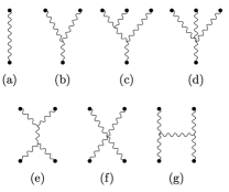
Figure 1: Feynman topologies to 3PM Kälin and Porto (2020a).

The EFT framework. The starting point is the effective action from which we derive the scattering trajectories. We proceed by integrating out the metric field $g_{\mu\nu}=\eta_{\mu\nu}+h_{\mu\nu}/M_{\rm Pl}$ (with $M_{\rm Pl}^{-1}\equiv\sqrt{32\pi G}$)

$$e^{iS_{\rm eff}}=\int{\cal D}h_{\mu\nu}\,e^{iS_{\rm EH}[h]+iS_{\rm GF}[h]+iS_{\rm pp}[x_{a},h]}\,,$$ (1)

in the (classical) saddle-point and weak-field approximations. We work with the Einstein-Hilbert action, $S_{\rm EH}$, and the convention $\eta_{\mu\nu}={\rm diag}(+,-,-,-)$. The gauge-fixing, $S_{\rm GF}$, is adjusted to simplify the Feynman rules Kälin and Porto (2020a). We use the (Polyakov) point-particle effective action,

$$S_{\rm pp}=-\sum_{a=1,2}\frac{m_{a}}{2}\int{\mathrm{d}}\tau_{a}\,g_{\mu\nu}(x^{\alpha}_{a})v_{a}^{\mu}v_{a}^{\nu}+\cdots\,,$$ (2)

with $\tau_{a}$ the proper time. The ellipses include higher-derivative terms accounting for finite-size effects and counterterms to remove (classical) ultraviolet divergences Goldberger and Rothstein (2006a); Kälin and Porto (2020a). As usual, we use dimensional regularization.

Impulse from Action. From the action we read off the effective Lagrangian at each order in $G$: ${\cal L}_{\rm eff}={\cal L}_{0}+{\cal L}_{1}+{\cal L}_{2}+{\cal L}_{3}+\cdots$. Although it may be non-local in time when radiation-reaction effects are included Damour et al. (2014); Galley et al. (2016), it is manifestly local with only potential modes Kälin and Porto (2020a). Using the effective Lagrangian we obtain the trajectories,

$$x^{\mu}_{a}(\tau_{a}) =b^{\mu}_{a}+u^{\mu}_{a}\tau_{a}+\sum_{n}\delta^{(n)}x^{\mu}_{a}(\tau_{a})\,,$$ (3)

with $u^{\mu}_{a}$ the velocity at infinity, obeying $u_{a}^{2}=1$, and $b^{\mu}\equiv b^{\mu}_{1}-b_{2}^{\mu}$ the impact parameter. For instance, at LO,

$$\delta^{(1)}x^{\mu}_{1}(\tau_{1})=- \frac{m_{2}}{8M_{\rm Pl}^{2}}\big{(}(2\gamma^{2}-1)\eta^{\mu\nu}-2(2\gamma u_{2}^{\mu}-u_{1}^{\mu})u_{1}^{\nu}\big{)}$$

$$\times\int_{k}\frac{ik_{\nu}\,\hat{\delta}(k\cdot u_{2})\,e^{ik\cdot b}}{k^{2}(k\cdot u_{1}-i0^{+})^{2}}e^{i(k\cdot u_{1}-i0^{+})\tau_{1}}.$$ (4)

We use the notation $\int_{k}\equiv\int\frac{{\mathrm{d}}^{4}k}{(2\pi)^{4}}$, $\hat{\delta}(x)\equiv 2\pi\delta(x)$ and

$$\gamma\equiv u_{1}\cdot u_{2}=\frac{p_{1}\cdot p_{2}}{m_{1}m_{2}}=\frac{E_{1}E_{2}+{\bm{p}}^{2}}{m_{1}m_{2}}\,,$$ (5)

where $E_{a}=\sqrt{{\bm{p}}^{2}+m_{a}^{2}}$ and $\pm{\bm{p}}$ is the incoming CoM momentum. Notice the factor of $(k\cdot u_{1}-i0^{+})^{-1}$, with the $i0^{+}$ to ensure convergence of the time integrals, which resembles the linear propagators appearing in heavy-quark effective theory Grinstein (1991). The pole shifts to $(k\cdot u_{2}+i0^{+})^{-1}$ for particle 2. The impulse follows from the effective action,

$$\Delta p_{a}^{\mu}=-\eta^{\mu\nu}\int_{-\infty}^{+\infty}{\mathrm{d}}\tau_{a}\frac{\partial{\cal L_{\rm eff}}}{\partial x^{\nu}_{a}}(x_{a}(\tau_{a}))\,,$$ (6)

where the overall sign is due to our conventions. The impulse can then be solved iteratively, starting with the undeflected trajectory in (3). Notice that all of the ${\cal L}_{k<n}$’s contribute to $n$PM order, and must be evaluated on the trajectories up to $(n{-}k)$-th order in $G$. We refer to this procedure as iterations Kälin and Porto (2020a). The scattering angle,

$$\frac{\chi}{2}=\sum_{n}\chi^{(n)}_{b}\left(\frac{GM}{b}\right)^{n}=\sum_{n}\frac{\chi^{(n)}_{j}}{j^{n}}\,,$$ (7)

with $1/j=GM\mu/(p_{\infty}b)$, is obtained from the relation

$$2\sin\frac{\chi}{2}=2\left(\frac{\chi}{2}-\frac{1}{6}\left(\frac{\chi}{2}\right)^{3}+\cdots\right)=\frac{\sqrt{-\Delta p_{a}^{2}}}{p_{\infty}}\,,$$ (8)

where

$$p_{\infty}=\mu\frac{\sqrt{\gamma^{2}-1}}{\Gamma}\,,\,\,\Gamma\equiv\frac{E}{M}=\sqrt{1+2\nu(\gamma-1)}\,,$$ (9)

with $E,M$ the total mass and energy, respectively. We use the notation $\mu=m_{1}m_{2}/M$ for the reduced mass, and $\nu=\mu/M$ for the symmetric mass ratio.The impulse may be further split into a contribution along the direction of the impact parameter as well as a term proportional to the velocities Kälin and Porto (2020a). Due to momentum conservation and the on-shell condition, we have

$$(p_{a}+\Delta p_{a})^{2}=p_{a}^{2}\,\,\Longrightarrow\,\,2p_{a}\cdot\Delta p_{a}=-\Delta p_{a}^{2}.$$ (10)

Moreover, since $\Delta^{(1)}p_{1}^{\mu}\propto b^{\mu}$ at leading PM order Kälin and Porto (2020a), and $b\cdot u_{a}=0$, we can use (10) to solve iteratively for the component along the velocities. This allows us to restrict the derivation of the impulse to the perpendicular plane Kälin and Porto (2020a). Feynman Integrals. To 3PM order the Feynman topologies are shown in Fig. 1. The computation yields four-dimensional relativistic integrals constrained by a series of $\delta$-functions, $\delta(k_{i}\cdot u_{a})$, which arise due to the time integration in (6) after inputting (3). Moreover, in addition to the standard factors of $1/k^{2}$ from the gravitational field, we have linear propagators, as in (Conservative Dynamics of Binary Systems to Third Post-Minkowskian Order from the Effective Field Theory Approach), which are needed to compute the iterations. As we mentioned, we restrict ourselves to the computation of the impulse in the direction of the impact parameter. The derivation is then reduced to a series of terms proportional to the Fourier transform in the ‘transfer momentum’,

$$\int_{q}\hat{\delta}(q\cdot u_{1})\hat{\delta}(q\cdot u_{2})\,iq^{\mu}\,t^{s}\,M^{(a,\tilde{a})}_{n_{1}n_{2};i_{1}\cdots i_{5}}(q,\gamma)e^{iq\cdot b}\,,$$ (11)

where the factor of $t^{s}$, with $t\equiv-q^{2}$, depends on the tensor reduction of the given diagram. We find the following (cut) ‘two loop’ integrals Kälin et al.

$$M^{(a,\tilde{a})}_{n_{1}n_{2};i_{1}\cdots i_{5}}(q,\gamma)\equiv\int_{k_{1},k_{2}}\frac{\hat{\delta}(k_{1}\cdot u_{a})\hat{\delta}(k_{2}\cdot u_{\tilde{a}})}{A_{1,\not a}^{n_{1}}A_{2,\not\tilde{a}}^{n_{2}}\,D_{1}^{i_{1}}\cdots D_{5}^{i_{5}}}\,,$$ (12)

are sufficient to 3PM order, where ($\not 1=2$, $\not 2=1$)

$$\begin{aligned} &A_{1,\not a}=k_{1}\cdot u_{\not a},\,A_{2,\not\tilde{a}}=k_{2}\cdot u_{\not{\tilde{a}}},\,D_{1}=k_{1}^{2},\,D_{2}=k_{2}^{2}\,,\\[3.50006pt] &D_{3}=(k_{1}{+}k_{2}{-}q)^{2},\,D_{4}=(k_{1}{-}q)^{2},\,D_{5}=(k_{2}{-}q)^{2}.\end{aligned}$$ (13)

All the integrals we encounter in our computation, including the iterations, can be embedded into the family in (12) with different choices of $(a,\tilde{a})$. The $i0$-prescription is such the $u_{1,2}$ are always accompanied by $\mp i0^{+}$, as in (Conservative Dynamics of Binary Systems to Third Post-Minkowskian Order from the Effective Field Theory Approach). The other cases are obtained by different symmetrizations Kälin et al. . We keep only non-analytic terms in $t$ which yield long-range interactions Kälin and Porto (2020a). We outline the integration procedure momentarily. The outcome is the scaling

$$t^{s}M^{(a,\tilde{a})}_{n_{1}n_{2};i_{1}\cdots i_{5}}\,\propto\,{1\over\epsilon}\,t^{-2\epsilon}\,,$$ (14)

with $\epsilon=(4-D)/2$, which gives for the impulse in (11) the expected $b^{\mu}/b^{4}$ in $D=4$. The poles (and $\log\bar{\mu}$’s) in dimensional regularization accompanying the $\log t$’s produce contact terms that neatly drop out without referring to subtraction schemes Kälin and Porto (2020a).

Potential Modes. In the framework of the PN expansion, the integrals would be performed using a mode factorization into potential $(k_{0}\ll|{\bm{k}}|)$ and radiation $(k_{0}\sim|{\bm{k}}|)$ modes, while keeping manifest power counting in the velocity Goldberger and Rothstein (2006a); Beneke and Smirnov (1998); Porto (2016b). The computation with potential modes then reduces to a series of three-dimensional (massless) integrals. In contrast, in the PM scheme we ought to keep the propagators fully relativistic. The associated Feynman integral still receive contributions from both potential and radiation modes (yielding real and imaginary parts). We are interested here in the conservative sector, and we ignore for now radiation-reaction effects. As discussed in Kälin and Porto (2020a), to isolate the potential modes we adapt to our EFT framework the powerful tools developed in Bern et al. (2019a, b); Parra-Martinez et al. (2020). Notably, we make use of the methodology of differential equations using boundary conditions from the (static) limit $\gamma\to 1$ Parra-Martinez et al. (2020).On the one hand, for diagrams $(c)$ and $(d)$ in Fig. 1, only the $M^{(1,1)}_{n_{1},n_{2};\cdots}$ in (12) are needed, with $(n_{1},n_{2})\leq 0$, plus mirror images. These integrals, which contribute to the one-point function of a (boosted) Schwarzschild background, can be computed in the rest frame

$$u_{1}=(1,0,0,0)\,,\,\,u_{2}=(\gamma,\gamma\beta,0,0)\,,$$ (15)

with $\beta\gamma=\sqrt{\gamma^{2}-1}$ Kälin and Porto (2020a). At the end of the day, they turn into the same type that appear in the static limit of the PN expansion, see e.g. Gilmore and Ross (2008). For diagrams ($e$), $(f)$ and $(g)$ in Fig. 1, on the other hand, the $M^{(1,2)}_{n_{1}n_{2};\cdots}$ are required instead, also with $(n_{1},n_{2})\leq 0$. Remarkably, the associated integrals for all these diagrams can be decomposed into a basis involving only the $M^{(1,2)}_{00;\cdots}$ subset Kälin et al. . Furthermore, using integration by part (IBP) relationships Chetyrkin and Tkachov (1981); Tkachov (1981), the contribution from diagrams $(e)$ and $(f)$ in Fig. 1 reduces to integrals with $i_{3}=0$. It is then straightforward to show that both diagrams vanish in $D=4$. (This is reminiscent of the fact that they do not enter at 2PN either Gilmore and Ross (2008).) Using the IBP relations and the aid of FIRE6 Smirnov and Chuharev (2019) and LiteRed Lee (2012), as well as symmetry arguments, the calculation of the remaining (so-called $H$) diagram in Fig.1 (g) is reduced to the following basis Kälin et al.

$$\left\{I_{11111},I_{11211},I_{01101},I_{11011},I_{00211},I_{00112},I_{00111}\right\},$$ (16)

with $I_{i_{1}\cdots i_{5}}\equiv M^{(1,2)}_{00;i_{1}\cdots i_{5}}$. For the computation we follow Henn (2013) and various tools, e.g. epsilon Prausa (2017), to construct a canonical basis $\vec{h}=\{h_{n=1\cdots 7}\}$ such that the velocity dependence is obtained via differential equations,

$$\partial_{x}\vec{h}(x,\epsilon)\,=\,\epsilon\,\mathbb{M}(x)\,\vec{h}(x,\epsilon)\,$$ (17)

with $\gamma=(x^{2}+1)/(2x)$, as advocated in Parra-Martinez et al. (2020). Because the set in (16) contains up to five (quadratic) propagators only, the associated boundary conditions in our case are then reduced to the same type of integrals that appear in the PN regime at two loops (Kite diagrams, e.g. Foffa et al. (2017)). It turns out only a handful contribute to the $H$ diagram in $D=4$, featuring the much anticipated factor of $\log x$ observed in Bern et al. (2019a, b); Parra-Martinez et al. (2020).

To complete the derivation we have to include the iterations. Surprisingly, the set in (16) is (almost) sufficient for all the contributions. For instance, iterations involving the deflection due to Fig.1 $(a)$ at LO order for the impulse due to Fig. 1 $(b)$, and vice verse, follow from (16). Yet, for the deflection from Fig.1 $(a)$ to NLO additional integrals are needed, resembling other (cut) topologies in Bern et al. (2019b); Parra-Martinez et al. (2020). In our case, we need the following two:

$$\{M^{(1,1)}_{11;11100}\,,\,\,M^{(1,2)}_{11;11100}\}\,.$$ (18)

Due to the presence of divergences, however, their computation is somewhat subtle. For the first one we can readily go to the rest frame in (15) producing a $D-1$ integral. We then use the symmetrization described in Parra-Martinez et al. (2020). Alternatively, it may be computed using the prescription in Cheung et al. (2018); Bern et al. (2019a, b) in the $u_{2}$-frame. Both can be adapted to all $\pm i0$ choices. The result is proportional to (twice) the standard one loop bubble integrals with static PN sources Gilmore and Ross (2008), although in $D-2$ dimensions. The same trick does not apply to the latter, but it can be easily incorporated into the canonical basis to obtain its $\gamma$-dependence. Yet, due to a divergence in the static limit, we need some care with the boundary condition. This is accounted for in the canonical basis by pulling out the relevant factor of $\beta$ (and $\epsilon$). Once again we perform the integral in the rest frame, expand in small velocity and retain the leading term in $1/\beta$. In this limit, the $M^{(1,2)}_{11;\ldots}$ integral turns out to be equivalent (modulo different $\pm i0$ choices) to the $M^{(1,1)}_{11;\ldots}$ counterpart. We have checked all these relationships explicitly via a standard $\alpha$-parameterization Smirnov (2012). At the end, as expected, the associated divergences cancel out in the final answer without subtractions.The above steps culminate the derivation of the master integrals in the potential region via differential equations. Using various arguments, the boundary conditions are reduced to the master integrals that appear in the static limit of the PN expansion at the same loop order. See Kälin et al. for a more detailed discussion.

Scattering data. The result for the impulse now follows from basic algebraic manipulations, and we arrive at

$$\Delta^{\!(3)}p_{1}^{\mu}=\, \frac{G^{3}b^{\mu}}{|b^{2}|^{2}}\Bigg{(}\frac{16m_{1}^{2}m_{2}^{2}(4\gamma^{4}-12\gamma^{2}-3)\operatorname{sinh^{-1}}\sqrt{\frac{\gamma-1}{2}}}{(\gamma^{2}-1)}$$

$$-\frac{4m_{1}^{2}m_{2}^{2}\gamma(20\gamma^{6}-90\gamma^{4}+120\gamma^{2}-53)}{3(\gamma^{2}-1)^{5/2}}$$

$$-\frac{2m_{1}m_{2}(m_{1}^{2}+m_{2}^{2})(16\gamma^{6}{-}32\gamma^{4}{+}16\gamma^{2}{-}1)}{(\gamma^{2}-1)^{5/2}}\Bigg{)}$$

$$+\frac{3\pi}{2}\frac{\left(2\gamma^{2}-1\right)(5\gamma^{2}-1)}{(\gamma^{2}-1)^{2}}\frac{G^{3}M^{2}\mu}{|b^{2}|^{3/2}}$$

$$\quad\times\Big{(}(\gamma m_{2}+m_{1})u_{2}^{\mu}-(\gamma m_{1}+m_{2})u_{1}^{\mu}\Big{)}.$$ (19)

The last term, which does not feature in the deflection angle at this order, is obtained from (10) and the result in Kälin and Porto (2020a). Hence, using (8), the 1PM angle (cube) and the 2PM impulse along the velocities in Kälin and Porto (2020a), we find

$$\frac{\chi^{(3)}_{b}}{\Gamma}=\, \frac{1}{(\gamma^{2}-1)^{3/2}}\Bigg{[}-\frac{4\nu}{3}\gamma\sqrt{\gamma^{2}-1}(14\gamma^{2}+25)$$

$$+\frac{(64\gamma^{6}-120\gamma^{4}+60\gamma^{2}-5)(1+2\nu(\gamma-1))}{3(\gamma^{2}-1)^{3/2}}$$

$$-8\nu(4\gamma^{4}-12\gamma^{2}-3)\operatorname{sinh^{-1}}\sqrt{\frac{\gamma-1}{2}}\,\Bigg{]}\,,$$ (20)

which, using $\chi_{j}^{(3)}=(p_{\infty}/\mu)^{3}\chi_{b}^{(3)}=\big{(}\sqrt{\gamma^{2}-1}/\Gamma\big{)}^{3}\chi_{b}^{(3)}$, is in agreement with the derivation in Bern et al. (2019a, b), see also Antonelli et al. (2019).

B2B map. The scattering data allows us to construct the (reduced) radial action Kälin and Porto (2020b, c)

$$i_{r}=\frac{p_{\infty}}{\sqrt{-p_{\infty}^{2}}}\chi^{(1)}_{j}-j\left(1+\frac{2}{\pi}\sum_{n=1}^{\infty}\frac{\chi^{(2n)}_{j}}{(1-2n)j^{2n}}\right)\,,$$ (21)

via analytic continuation to $\gamma<1$. As we discussed in Kälin and Porto (2020b, c), the natural power counting in $1/j$ in the PM expansion requires the (so far unknown) $\chi^{(4)}_{j}$ coefficient. The latter can be written, using the results in Kälin and Porto (2020b, c), as

$$\chi^{(4)}_{j}=\frac{3\pi}{8M^{4}\mu^{4}}\Big{(}P_{1}P_{3}+\frac{1}{2}P_{2}^{2}+p_{\infty}^{2}P_{4}\Big{)}\,,$$ (22)

with the $P_{n}$’s from the expansion of the CoM momentum

$${\bm{p}}^{2}=p_{\infty}^{2}+\sum_{n=1}^{\infty}P_{n}(E)\left(\frac{G}{r}\right)^{n}\,.$$ (23)

The $P_{n}$’s can also be obtained from the scattering angle, as described in Kälin and Porto (2020b, c). For instance, inverting the relation

$$\chi_{j}^{(3)}=\frac{1}{M^{3}\mu^{3}p_{\infty}^{3}}\left(-\frac{P_{1}^{3}}{24}+p_{\infty}^{2}\frac{P_{1}P_{2}}{2}+p_{\infty}^{4}P_{3}\right)\,,$$ (24)

together with (20) and the results in Kälin and Porto (2020a), yields

$$\frac{P_{3}}{M^{3}\mu^{2}}=\Bigg{(}\frac{18\gamma^{2}-1}{2\Gamma}+\frac{8\nu}{\Gamma}(3{+}12\gamma^{2}{-}4\gamma^{4})\frac{\operatorname{sinh^{-1}}\sqrt{\frac{\gamma-1}{2}}}{\sqrt{\gamma^{2}-1}}+$$ (25)

$$\frac{\nu}{6\Gamma}\left(6{-}206\gamma{-}108\gamma^{2}{-}4\gamma^{3}+\frac{18\Gamma(1-2\gamma^{2})(1-5\gamma^{2})}{(1+\Gamma)(1+\gamma)}\right)\Bigg{)}\,.$$

This compact expression encodes all the information at 3PM order. It can be analytically continued to negative binding energies ($\gamma<1$) to derive observables for binary systems via the B2B map. Because of the factor of $p_{\infty}^{2}$ in (22), and since (23) has a well-defined static limit, the contribution in (21) from $P_{4}$ is subleading in the PN expansion. This allows us to perform a consistent PN-truncation by keeping the $P_{n\leq 3}$ terms in (22) (ignoring also higher orders in $1/j$ which are PN-suppressed). This is carried out in detail in Kälin and Porto (2020b, c), and shown to agree with the literature in the overlapping regime of validity.

Amplitude & Hamiltonian. It is instructive to use the B2B dictionary to also reconstruct both, the classical limit of the scattering amplitude as well as the Hamiltonian for the two-body system in the CoM (isotropic) frame. Using the relationship found in Kälin and Porto (2020b),

$${\bm{p}}^{2}=p_{\infty}^{2}+\frac{1}{2E}\int{\mathrm{d}}^{3}{\bm{r}}{\cal M}(p_{\infty},{\bm{q}})e^{i{\bm{q}}\cdot{\bm{r}}},$$ (26)

we immediately read off from (25) the (infrared-finite part of the) scattering amplitude in the classical limit, which agrees with the result in Bern et al. (2019b) (see Eq. (9.3)). For the PM expansion of the Hamiltonian,

$$H(r,{\bm{p}}^{2})=\sum_{i}\frac{c_{i}({\bm{p}}^{2})}{i!}\left(\frac{G}{r}\right)^{i}\,,$$ (27)

the coefficients can also be expressed iteratively in terms of the $P_{n}$’s in (23) Kälin and Porto (2020b). To 3PM order we find

$$\frac{c_{3}({\bm{p}})}{3!}= -\frac{P_{3}(E)}{2E\xi}+\frac{(3\xi-1)P_{2}(E)P_{1}(E)}{4E^{3}\xi^{3}}$$

$$+\frac{(P_{2}(E)P^{\prime}_{1}(E)+P^{\prime}_{2}(E)P_{1}(E))}{4E^{2}\xi^{2}}$$

$$-\frac{(5\xi^{2}-5\xi+1)P_{1}^{3}(E)}{16E^{5}\xi^{5}}-\frac{(9\xi-3)P_{1}^{2}(E)P^{\prime}_{1}(E)}{16E^{4}\xi^{4}}$$

$$-\frac{P_{1}^{2}(E)P^{\prime\prime}_{1}(E)}{16E^{3}\xi^{3}}-\frac{P_{1}(E)(P^{\prime}_{1}(E))^{2}}{8E^{3}\xi^{3}}\,,$$ (28)

where prime denotes a derivative with respect to $E$, and $\xi\equiv E_{1}E_{2}/(E_{1}+E_{2})^{2}$. Inputting (25), and $P_{1,2}$ from the 2PM results Kälin and Porto (2020a), we exactly reproduce the $c_{3}$ in Bern et al. (2019a, b). Notice, however, that the relevant PM information to compute observables through the B2B map is (more succinctly) encoded in (25) at two loops, and ultimately the (yet to be computed) scattering angle at 4PM order.

Conclusions. Using the EFT approach and B2B dictionary Kälin and Porto (2020b, c, a), we derived the conservative dynamics for non-spinning binary systems to 3PM order. Our results, purely within the classical realm, are in perfect agreement with those reported in Bern et al. (2019a, b), thus removing the objections raised in Damour (2019) against their validity. Even though, unlike the approach in Bern et al. (2019a, b), our derivation entails the use of Feynman diagram, because of the simplifications of the EFT/B2B framework just a handful are required (two of which are zero) at this order, see Fig. 1. Moreover, only massless integrals appear and, as it was already illustrated in Kälin and Porto (2020a), we do not encounter the (super-classical) infrared singularities which have, thus far, polluted the extraction of classical physics from the amplitudes program. By adapting to our EFT approach the methods in Cheung et al. (2018); Bern et al. (2019a, b); Parra-Martinez et al. (2020), we found that the contribution from potential modes to the master integrals can be computed to all orders in velocities using differential equations (without the need of the PN-type resummations in Bern et al. (2019a, b)). Remarkably, the boundary conditions are obtained from the knowledge of the same master integrals which appear in the static limit with PN sources to two loops, albeit in $D-1$ and $D-2$ dimensions. This implies that the PM dynamics can be bootstrapped from PN information (at least to NNLO). This is not surprising for the evaluation on the unperturbed trajectory, which serves as a stationary limit of the PM regime, but strikingly the same occurs for the iterations. Since master integrals for the PN expansion are known to four loops Foffa et al. (2017), bootstrapping integrals through differential equations could potentially give us up to the 5PM order.We note also that the infusion of data from outside of PN/PM schemes can further simplify the computation. For instance, the test-particle limit in a Schwarzschild background provides us the value of the $M^{(1,1)}$ master integrals in the iterations. In turn, these are related to the $M^{(1,2)}$ family in the static limit. This would then allow us to read off their boundary condition directly from the test-body limit, and subsequently the entire velocity dependence with the differential equations. The fact that we get extra mileage from the probe limit is not surprising Kälin and Porto (2020b). What is remarkable, and more so due to the lack of crossing symmetry, is the connection to ${\cal O}(\nu)$ corrections through the static limit and differential equations. Likewise, information from the gravitational self-force program Barack and Pound (2019); Pound et al. (2020) may be also used to aid the calculation in the PM expansion, e.g. Damour (2016, 2018); Antonelli et al. (2019); Bini et al. (2019); Damour (2019); Bini et al. (2020b, a); Vines et al. (2018); Siemonsen and Vines (2019); Bini et al. (2020c). Irrespectively of the weapon of choice, the B2B dictionary Kälin and Porto (2020b, c) is imploring us to continue to even higher orders. The derivation of the needed 4PM scattering angle is ongoing in the EFT approach, which we have demonstrated here is a powerful framework, not only for PN calculations Goldberger and Rothstein (2006a); Goldberger (2007); Foffa and Sturani (2014); Rothstein (2014); Cardoso and Porto (2014); Porto (2016b), but also in the PM regime Kälin and Porto (2020a); Kälin et al. (2020).

Acknowledgements. We thank Babis Anastasiou, Zvi Bern, Clifford Cheung, Lance Dixon, Claude Duhr, Julio Parra-Martinez, Radu Roiban, Chia-Hsien Shen, Mikhail Solon, Gang Yang and Mao Zeng for useful discussions. We are grateful to Julio Parra-Martinez and Mao Zeng for helpful comments on the integration in the potential region. R.A.P. acknowledges financial support from the ERC Consolidator Grant “Precision Gravity: From the LHC to LISA” provided by the European Research Council (ERC) under the European Union’s H2020 research and innovation programme (grant agreement No. 817791). Z.L. and R.A.P. are also supported by the Deutsche Forschungsgemeinschaft (DFG) under Germany’s Excellence Strategy (EXC 2121) ‘Quantum Universe’ (390833306). G.K. is supported by the Knut and Alice Wallenberg Foundation under grant KAW 2018.0441, and in part by the US DoE under contract DE-AC02-76SF00515.

References

- Kälin and Porto (2020a) G. Kälin and R. A. Porto, (2020a), arXiv:2006.01184 .
- Kälin and Porto (2020b) G. Kälin and R. A. Porto, JHEP 01, 072 (2020b), arXiv:1910.03008 .
- Kälin and Porto (2020c) G. Kälin and R. A. Porto, JHEP 02, 120 (2020c), arXiv:1911.09130 .
- Bern et al. (2019a) Z. Bern, C. Cheung, R. Roiban, C.-H. Shen, M. P. Solon, and M. Zeng, Phys. Rev. Lett. 122, 201603 (2019a), arXiv:1901.04424 .
- Bern et al. (2019b) Z. Bern, C. Cheung, R. Roiban, C.-H. Shen, M. P. Solon, and M. Zeng, JHEP 10, 206 (2019b), arXiv:1908.01493 .
- Abbott et al. (2019a) B. P. Abbott et al. (LIGO Scientific, Virgo), Phys. Rev. X9, 031040 (2019a), arXiv:1811.12907 .
- Abbott et al. (2019b) R. Abbott et al. (LIGO Scientific, Virgo), (2019b), arXiv:1912.11716 .
- Buonanno and Sathyaprakash (2014) A. Buonanno and B. Sathyaprakash, (2014), arXiv:1410.7832 .
- Porto (2016a) R. A. Porto, Fortsch. Phys. 64, 723 (2016a), arXiv:1606.08895 .
- Porto (2017a) R. A. Porto, (2017a), arXiv:1703.06440 [physics.pop-ph] .
- Blanchet (2014) L. Blanchet, Living Reviews in Relativity 17, 2 (2014).
- Schäfer and Jaranowski (2018) G. Schäfer and P. Jaranowski, Living Rev. Rel. 21, 7 (2018), arXiv:1805.07240 .
- Damour et al. (2014) T. Damour, P. Jaranowski, and G. Schäfer, Phys. Rev. D 89, 064058 (2014), arXiv:1401.4548 .
- Jaranowski and Schäfer (2015) P. Jaranowski and G. Schäfer, Phys. Rev. D92, 124043 (2015), arXiv:1508.01016 .
- Bernard et al. (2016) L. Bernard, L. Blanchet, A. Bohe, G. Faye, and S. Marsat, Phys. Rev. D 93, 084037 (2016), arXiv:1512.02876 .
- Bernard et al. (2017) L. Bernard, L. Blanchet, A. Bohe, G. Faye, and S. Marsat, Phys. Rev. D96, 104043 (2017), arXiv:1706.08480 .
- Marchand et al. (2018) T. Marchand, L. Bernard, L. Blanchet, and G. Faye, Phys. Rev. D 97, 044023 (2018), arXiv:1707.09289 .
- Goldberger and Rothstein (2006a) W. D. Goldberger and I. Z. Rothstein, Phys. Rev. D73, 104029 (2006a), arXiv:hep-th/0409156 .
- Goldberger (2007) W. D. Goldberger, in Les Houches Summer School - Session 86 (2007) arXiv:hep-ph/0701129 .
- Foffa and Sturani (2014) S. Foffa and R. Sturani, Class. Quant. Grav. 31, 043001 (2014), arXiv:1309.3474 .
- Rothstein (2014) I. Rothstein, Gen. Rel. Grav. 46, 1726 (2014).
- Cardoso and Porto (2014) V. Cardoso and R. A. Porto, Gen. Rel. Grav. 46, 1682 (2014), arXiv:1401.2193 .
- Porto (2016b) R. A. Porto, Phys. Rept. 633, 1 (2016b), arXiv:1601.04914 .
- Elvang and Huang (2015) H. Elvang and Y.-t. Huang, Scattering Amplitudes in Gauge Theory and Gravity (Cambridge University Press, 2015).
- Bern et al. (2019c) Z. Bern, J. J. Carrasco, M. Chiodaroli, H. Johansson, and R. Roiban, (2019c), arXiv:1909.01358 .
- Gilmore and Ross (2008) J. B. Gilmore and A. Ross, Phys. Rev. D 78, 124021 (2008), arXiv:0810.1328 .
- Foffa and Sturani (2011) S. Foffa and R. Sturani, Phys. Rev. D 84, 044031 (2011), arXiv:1104.1122 .
- Foffa and Sturani (2013) S. Foffa and R. Sturani, Phys. Rev. D 87, 064011 (2013), arXiv:1206.7087 .
- Galley et al. (2016) C. Galley, A. Leibovich, R. A. Porto, and A. Ross, Phys. Rev. D 93, 124010 (2016), arXiv:1511.07379 .
- Foffa et al. (2017) S. Foffa, P. Mastrolia, R. Sturani, and C. Sturm, Phys. Rev. D 95, 104009 (2017), arXiv:1612.00482 .
- Porto and Rothstein (2017) R. A. Porto and I. Rothstein, Phys. Rev. D 96, 024062 (2017), arXiv:1703.06433 .
- Foffa and Sturani (2019) S. Foffa and R. Sturani, Phys. Rev. D 100, 024047 (2019), arXiv:1903.05113 .
- Foffa et al. (2019a) S. Foffa, R. A. Porto, I. Rothstein, and R. Sturani, Phys. Rev. D100, 024048 (2019a), arXiv:1903.05118 .
- Cheung et al. (2018) C. Cheung, I. Z. Rothstein, and M. P. Solon, Phys. Rev. Lett. 121, 251101 (2018), arXiv:1808.02489 .
- Foffa et al. (2019b) S. Foffa, P. Mastrolia, R. Sturani, C. Sturm, and W. J. Torres Bobadilla, Phys. Rev. Lett. 122, 241605 (2019b), arXiv:1902.10571 .
- Blümlein et al. (2020a) J. Blümlein, A. Maier, and P. Marquard, Phys. Lett. B 800, 135100 (2020a), arXiv:1902.11180 .
- Blümlein et al. (2020b) J. Blümlein, A. Maier, P. Marquard, and G. Schäfer, Phys. Lett. B 807, 135496 (2020b), arXiv:2003.07145 .
- Bini et al. (2020a) D. Bini, T. Damour, and A. Geralico, (2020a), arXiv:2004.05407 .
- Goldberger and Rothstein (2006b) W. Goldberger and I. Rothstein, Phys. Rev. D 73, 104030 (2006b), arXiv:hep-th/0511133 .
- Goldberger and Ross (2010) W. D. Goldberger and A. Ross, Phys. Rev. D81, 124015 (2010), arXiv:0912.4254 .
- Ross (2012) A. Ross, Phys. Rev. D85, 125033 (2012), arXiv:1202.4750 .
- Galley and Leibovich (2012) C. R. Galley and A. K. Leibovich, Phys. Rev. D 86, 044029 (2012), arXiv:1205.3842 .
- Leibovich et al. (2020) A. K. Leibovich, N. T. Maia, I. Z. Rothstein, and Z. Yang, Phys. Rev. D 101, 084058 (2020), arXiv:1912.12546 .
- Porto (2006) R. A. Porto, Phys. Rev. D 73, 104031 (2006), arXiv:gr-qc/0511061 .
- Porto and Rothstein (2006) R. A. Porto and I. Rothstein, Phys. Rev. Lett. 97, 021101 (2006), arXiv:gr-qc/0604099 .
- Porto and Rothstein (2007) R. A. Porto and I. Z. Rothstein, (2007), arXiv:0712.2032 .
- Porto (2008) R. A. Porto, Phys. Rev. D 77, 064026 (2008), arXiv:0710.5150 .
- Porto and Rothstein (2008a) R. A. Porto and I. Z. Rothstein, Phys.Rev. D78, 044012 (2008a), arXiv:0802.0720 .
- Porto and Rothstein (2008b) R. A. Porto and I. Z. Rothstein, Phys.Rev. D78, 044013 (2008b), arXiv:0804.0260 .
- Porto (2010) R. A. Porto, Class. Quant. Grav. 27, 205001 (2010), arXiv:1005.5730 .
- Porto et al. (2011) R. A. Porto, A. Ross, and I. Z. Rothstein, JCAP 1103, 009 (2011), arXiv:1007.1312 .
- Porto et al. (2012) R. A. Porto, A. Ross, and I. Z. Rothstein, JCAP 1209, 028 (2012), arXiv:1203.2962 .
- Maia et al. (2017a) N. T. Maia, C. R. Galley, A. K. Leibovich, and R. A. Porto, Phys. Rev. D 96, 084064 (2017a), arXiv:1705.07934 .
- Maia et al. (2017b) N. T. Maia, C. R. Galley, A. K. Leibovich, and R. A. Porto, Phys. Rev. D 96, 084065 (2017b), arXiv:1705.07938 .
- Levi and Steinhoff (2016) M. Levi and J. Steinhoff, (2016), arXiv:1607.04252 .
- Levi et al. (2020a) M. Levi, A. J. Mcleod, and M. Von Hippel, (2020a), arXiv:2003.02827 .
- Levi et al. (2020b) M. Levi, A. J. Mcleod, and M. Von Hippel, (2020b), arXiv:2003.07890 .
- Vaidya (2015) V. Vaidya, Phys. Rev. D91, 024017 (2015), arXiv:1410.5348 .
- Guevara et al. (2019a) A. Guevara, A. Ochirov, and J. Vines, Phys. Rev. D 100, 104024 (2019a), arXiv:1906.10071 .
- Arkani-Hamed et al. (2020) N. Arkani-Hamed, Y.-t. Huang, and D. O’Connell, JHEP 01, 046 (2020), arXiv:1906.10100 .
- Chung et al. (2020) M.-Z. Chung, Y.-t. Huang, J.-W. Kim, and S. Lee, (2020), arXiv:2003.06600 .
- Bern et al. (2020a) Z. Bern, A. Luna, R. Roiban, C.-H. Shen, and M. Zeng, (2020a), arXiv:2005.03071 .
- Damour (2019) T. Damour, (2019), arXiv:1912.02139v1 .
- Antonelli et al. (2019) A. Antonelli, A. Buonanno, J. Steinhoff, M. van de Meent, and J. Vines, Phys. Rev. D99, 104004 (2019), arXiv:1901.07102 .
- Damour (2016) T. Damour, Phys. Rev. D94, 104015 (2016), arXiv:1609.00354 .
- Damour (2018) T. Damour, Phys. Rev. D97, 044038 (2018), arXiv:1710.10599 .
- Bini et al. (2019) D. Bini, T. Damour, and A. Geralico, Phys. Rev. Lett. 123, 231104 (2019), arXiv:1909.02375 [gr-qc] .
- Damour and Nagar (2016) T. Damour and A. Nagar, Lect. Notes Phys. 905, 273 (2016).
- Henn (2015) J. M. Henn, J. Phys. A 48, 153001 (2015), arXiv:1412.2296 .
- Parra-Martinez et al. (2020) J. Parra-Martinez, M. S. Ruf, and M. Zeng, (2020), arXiv:2005.04236 .
- Neill and Rothstein (2013) D. Neill and I. Z. Rothstein, Nucl. Phys. B877, 177 (2013), arXiv:1304.7263 .
- Kosower et al. (2019) D. A. Kosower, B. Maybee, and D. O’Connell, JHEP 02, 137 (2019), arXiv:1811.10950 .
- Maybee et al. (2019) B. Maybee, D. O’Connell, and J. Vines, JHEP 12, 156 (2019), arXiv:1906.09260 .
- Galley and Porto (2013) C. Galley and R. A. Porto, JHEP 11, 096 (2013), arXiv:1302.4486 .
- Holstein and Ross (2008) B. R. Holstein and A. Ross, (2008), arXiv:0802.0716 .
- Bjerrum-Bohr et al. (2014) N. Bjerrum-Bohr, J. F. Donoghue, and P. Vanhove, JHEP 02, 111 (2014), arXiv:1309.0804 .
- Guevara (2019) A. Guevara, JHEP 04, 033 (2019), arXiv:1706.02314 .
- Chung et al. (2019a) M.-Z. Chung, Y.-T. Huang, J.-W. Kim, and S. Lee, JHEP 04, 156 (2019a), arXiv:1812.08752 .
- Guevara et al. (2019b) A. Guevara, A. Ochirov, and J. Vines, JHEP 09, 056 (2019b), arXiv:1812.06895 .
- Goldberger and Ridgway (2018) W. D. Goldberger and A. K. Ridgway, Phys. Rev. D97, 085019 (2018), arXiv:1711.09493 .
- Caron-Huot and Zahraee (2019) S. Caron-Huot and Z. Zahraee, JHEP 07, 179 (2019), arXiv:1810.04694 .
- Bjerrum-Bohr et al. (2018) N. E. J. Bjerrum-Bohr et al., Phys. Rev. Lett. 121, 171601 (2018), arXiv:1806.04920 .
- Cristofoli et al. (2019) A. Cristofoli, N. E. J. Bjerrum-Bohr, P. H. Damgaard, and P. Vanhove, (2019), arXiv:1906.01579 .
- Bjerrum-Bohr et al. (2019) N. E. J. Bjerrum-Bohr, A. Cristofoli, and P. H. Damgaard, (2019), arXiv:1910.09366 .
- Chung et al. (2019b) M.-Z. Chung, Y.-T. Huang, and J.-W. Kim, (2019b), arXiv:1908.08463 .
- Bautista and Guevara (2019a) Y. F. Bautista and A. Guevara, (2019a), arXiv:1903.12419 .
- Bautista and Guevara (2019b) Y. F. Bautista and A. Guevara, (2019b), arXiv:1908.11349 .
- Koemans Collado et al. (2019) A. Koemans Collado, P. Di Vecchia, and R. Russo, Phys. Rev. D100, 066028 (2019), arXiv:1904.02667 .
- Brandhuber and Travaglini (2020) A. Brandhuber and G. Travaglini, JHEP 01, 010 (2020), arXiv:1905.05657 [hep-th] .
- Johansson and Ochirov (2019) H. Johansson and A. Ochirov, JHEP 09, 040 (2019), arXiv:1906.12292 .
- Aoude et al. (2020) R. Aoude, K. Haddad, and A. Helset, (2020), arXiv:2001.09164 .
- Cristofoli et al. (2020) A. Cristofoli, P. H. Damgaard, P. Di Vecchia, and C. Heissenberg, (2020), arXiv:2003.10274 .
- Bern et al. (2020b) Z. Bern, H. Ita, J. Parra-Martinez, and M. S. Ruf, (2020b), arXiv:2002.02459 .
- Cheung and Solon (2020a) C. Cheung and M. P. Solon, JHEP 06, 144 (2020a), arXiv:2003.08351 .
- Cheung and Solon (2020b) C. Cheung and M. P. Solon, (2020b), arXiv:2006.06665 .
- Accettulli Huber et al. (2020) M. Accettulli Huber, A. Brandhuber, S. De Angelis, and G. Travaglini, (2020), arXiv:2006.02375 [hep-th] .
- Grinstein (1991) B. Grinstein, in Workshop on High-energy Phenomenology (1991) p. 0161.
- (98) G. Kälin, Z. Liu, and R. A. Porto, In preparation, .
- Beneke and Smirnov (1998) M. Beneke and V. A. Smirnov, Nucl. Phys. B522, 321 (1998), arXiv:hep-ph/9711391 .
- Chetyrkin and Tkachov (1981) K. Chetyrkin and F. Tkachov, Nucl. Phys. B 192, 159 (1981).
- Tkachov (1981) F. Tkachov, Phys. Lett. B 100, 65 (1981).
- Smirnov and Chuharev (2019) A. Smirnov and F. Chuharev, (2019), arXiv:1901.07808 .
- Lee (2012) R. Lee, (2012), arXiv:1212.2685 .
- Henn (2013) J. M. Henn, Phys. Rev. Lett. 110, 251601 (2013), arXiv:1304.1806 .
- Prausa (2017) M. Prausa, Comput. Phys. Commun. 219, 361 (2017), arXiv:1701.00725 .
- Smirnov (2012) V. A. Smirnov, Analytic tools for Feynman integrals (Springer, 2012).
- Porto (2017b) R. A. Porto, Phys. Rev. D 96, 024063 (2017b), arXiv:1703.06434 .
- Barack and Pound (2019) L. Barack and A. Pound, Rept. Prog. Phys. 82, 016904 (2019), arXiv:1805.10385 .
- Pound et al. (2020) A. Pound, B. Wardell, N. Warburton, and J. Miller, Phys. Rev. Lett. 124, 021101 (2020), arXiv:1908.07419 .
- Bini et al. (2020b) D. Bini, T. Damour, and A. Geralico, (2020b), arXiv:2003.11891 .
- Vines et al. (2018) J. Vines, J. Steinhoff, and A. Buonanno, (2018), arXiv:1812.00956 .
- Siemonsen and Vines (2019) N. Siemonsen and J. Vines, (2019), arXiv:1909.07361 .
- Bini et al. (2020c) D. Bini, T. Damour, and A. Geralico, Phys. Rev. D 101, 044039 (2020c), arXiv:2001.00352 .
- Kälin et al. (2020) G. Kälin, Z. Liu, and R. A. Porto, (2020), arXiv:2008.06047 [hep-th] .