Abstract

We compute the static contribution to the gravitational interaction potential of two point masses in the velocity-independent five-loop (and 5th post-Newtonian) approximation to the harmonic coordinates effective action in a direct calculation. The computation is performed using effective field methods based on Feynman diagrams in momentum-space in $d=3-2\varepsilon$ space dimensions. We also reproduce the previous results including the 4th post-Newtonian order.

1 Introduction

The interpretation of the signals detected in gravitational wave interferometers like LIGO and VIRGO [1] requires a very accurate knowledge of the binary dynamics of large coalescing masses. This also applies to the planned projects like INDIGO, LISA Pathfinder and the Einstein telescope [2]. The increasing improvements of the detector sensitivity requires highly precise theoretical predictions.

Different approaches are used as the effective one-body formalism [3, 4, 5, 6, 7, 8], numerical relativity [9, 10, 11], the self-force formalism [12, 13], the post-Newtonian (PN) [14, 15, 16, 17, 18, 19, 20, 21, 22, 23, 25, 24, 26, 27, 28, 29, 30, 31, 32, 33, 34, 35, 36, 37, 39, 38, 40, 41, 42, 43, 44, 45, 46, 47, 48, 49, 50, 51] and post-Minkowskian approach [52, 53, 54, 55, 56, 57, 58, 59, 60, 6, 7, 61, 48, 62] and effective field theory methods [63, 64]; for surveys see Refs. [65, 66, 67, 68, 69, 70].

In this letter we calculate a first contribution to the fifth post-Newtonian approximation: the five-loop static gravitational interaction potential between two non-spinning point masses. The two-particle force receives a series of different higher order corrections, which can be parameterized by a small parameter $\epsilon$, cf. Ref. [65],

$$F=F_{N}+\sum_{k=1}^{\infty}\epsilon^{2k}F_{kPN}+\epsilon^{4}F_{SO}+\epsilon^{4}F_{QO}+\epsilon^{5}F_{RR}+\epsilon^{6}F_{1PNSO}+\epsilon^{6}F_{1PNQO}+\epsilon^{6}F_{OO}+\epsilon^{6}F_{SS}+\epsilon^{6}F_{TO}+...$$ (1)

Here $F_{N}$ denotes Newton’s force [71], $F_{kPN}$ is the $k$th post-Newtonian force, $F_{RR}$ the 2.5 PN radiation reaction force, $F_{SO}$ and $F_{1PNSO}$ etc. are the spin-orbit coupling force and their post-Newtonian corrections, $F_{QO}$ and $F_{1PNQO}$ etc. are the quadrupole-orbit coupling force and its post-Newtonian corrections. $F_{OO},F_{SS}$ and $F_{TO}$ denote the octupole-orbit coupling force, the spin-spin coupling force, and tidal-orbit coupling force, respectively. We will concentrate here on the post-Newtonian corrections of the attraction of two spinless masses in the following, using non-relativistic gravitational fields obtained by a temporal Kaluza-Klein reduction [99] followed by a Weyl rescaling [100]. The corresponding action has been derived in Ref. [36]. In the representation time derivatives of arbitrary order occur, which also introduce higher derivatives of the accelerations $a_{1(2)}$. Since the Lagrange density of General Relativity is of second order, these terms shall be eliminated by adding suitable double (multiple)-zero terms [23]. One aims on the terms of the order

$$\sim\frac{G_{N}^{k}}{r^{k}}m_{1}^{l}m_{2}^{k+1-l},\leavevmode\nobreak\ \leavevmode\nobreak\ \leavevmode\nobreak\ l\in[1,k],$$ (2)

where $(k-1)$ labels the $k$th post-Newtonian approximation. Here $G_{N}$ denotes Newton’s constant, $r=|\mathbf{r}|$ the distance of the two masses and $m_{1(2)}$ are the two point masses.

We calculate the contribution to the fifth post-Newtonian approximation in the static limit, i.e. leaving the velocity-dependent contributions for a later work. The virial theorem [101] relates $m_{1}\mathbf{v}_{1}^{2}+m_{2}\mathbf{v}_{2}^{2}\sim\frac{G_{N}}{r}m_{1}m_{2}$ on temporal average, where $\mathbf{v}_{1(2)}$ denote the velocities of the two point masses. Therefore velocity terms have to be considered at this order in general. This also applies to higher derivatives of the velocities, which can finally be mapped to terms $\propto(G_{N}^{k}/r^{k})v_{i}^{l}$ by applying the equation of motion.

We first outline the basic formalism and present then the details of the calculation. Finally, we compare to the results in the literature including the fourth post-Newtonian approximation.

2 Basic Formalism

The action of General Relativity for the present problem consists of the following three components,

$$S_{GR}=S_{\text{pp}}+S_{\text{EH}}+S_{\text{GF}}\,,$$ (3)

where $S_{\text{pp}},S_{\text{EH}}$ and $S_{\text{GF}}$ are the point-particle-, the Einstein-Hilbert- , [102], and the gauge fixing contributions. Following [36] we parameterize the Riemann metric by

$$g_{\mu\nu}=e^{2\phi/\Lambda}\begin{pmatrix}-1&A_{j}/\Lambda\\ A_{i}/\Lambda&e^{-c_{d}\phi/\Lambda}\gamma_{ij}-A_{i}A_{j}/\Lambda^{2}\end{pmatrix}\,.$$ (4)

Here, the scalar field $\phi$, 3-vector field $A_{i}$ and tensor field $\gamma_{ij}$ are introduced which parameterize the ten components of the metric tensor and $\Lambda$ and $c_{d}$ are given by

$$\Lambda^{-1} = \sqrt{32\pi G_{N}},$$ (5)

$$c_{d} = 2\frac{d-1}{d-2},$$ (6)

where $d:=3-2\varepsilon$ and $G_{N}\rightarrow G_{N}(\mu)^{3-d}$ in $d$ dimensions, with $\mu$ a mass scale. In the Newtonian limit of flat space–time we adopt the ‘mostly plus’ convention $g_{\mu\nu}\to\eta_{\mu\nu}=\operatorname{diag}(-1,+1,+1,+1)$, with $\eta_{\mu\nu}$ the Minkowskian metric. The contribution to the spatial metric $\gamma_{ij}$ is parameterized by

$$\gamma_{ij} = \delta_{ij}+\sigma_{ij}/\Lambda,$$ (7)

where $\delta_{ij}$ denotes Kronecker’s symbol. The gravitational field amplitude is given by

$$h^{\alpha\beta}=\sqrt{-g}g^{\alpha\beta}-\eta^{\alpha\beta}$$ (8)

and the harmonic coordinate condition reads

$$\partial_{\mu}h^{\alpha\mu}=0.$$ (9)

The point-particle action

$$S_{\text{pp}} = -\sum_{k=1}^{2}m_{k}\int d\tau_{k}=-\sum_{k=1}^{2}m_{k}\int dt\sqrt{-g_{\mu\nu}\frac{dx_{k}^{\mu}}{dt}\frac{dx_{k}^{\nu}}{dt}}$$ (10)

$$= -\sum_{k=1}^{2}m_{k}\int dte^{\phi/\Lambda}\sqrt{(1-\mathbf{A}.\mathbf{v}_{k})^{2}-e^{-c_{d}\phi/\Lambda}\gamma_{ij}v_{k}^{i}v_{k}^{j}}$$

describes the point masses themselves.

The dynamics of the metric in one temporal and $d$ spatial dimensions are captured by the Einstein-Hilbert action, [36],

$$S_{\text{EH}}=\frac{1}{16\pi G_{N}}\int d^{d}x\leavevmode\nobreak\ dt\sqrt{-g}R[g]=S^{(0)}(\gamma,A,\phi)+S^{(1)}(\gamma,A,\phi)+S^{(2)}(\gamma,A,\phi),$$ (11)

sorting w.r.t. the occurring number of time-derivatives. For the static contribution calculated in the present paper only $S^{(0)}$ is relevant.

$$S^{(0)}(\gamma,A,\phi) = -\frac{1}{16\pi G_{N}}\int d^{d}x\leavevmode\nobreak\ dt\sqrt{\gamma}\Biggl{[}-R[\gamma]+\frac{1}{2}c_{d}\gamma^{ij}\partial_{i}\phi\partial_{j}\phi-\frac{1}{4}e^{c_{d}\phi}\gamma^{ik}\gamma^{jl}F_{ij}F_{kl}\Biggr{]},$$ (12)

where $R[\gamma]$ denotes the Ricci scalar and $F_{ij}=\partial_{i}A_{j}-\partial_{i}A_{j}$. The determinant $\gamma$ may be represented by

$$\gamma = 1+\sum_{k=1}^{\infty}\frac{\hat{\sigma}_{k}}{\Lambda^{k}}=1+\frac{1}{\Lambda}\text{tr}(\sigma)+\frac{1}{2\Lambda^{2}}\left[\text{tr}^{2}(\sigma)-\text{tr}\left(\sigma^{2}\right)\right]+\frac{1}{6\Lambda^{3}}\left[\text{tr}^{3}(\sigma)+2\text{tr}\left(\sigma^{3}\right)\right.$$ (13)

$$\left.-3\text{tr}\left(\sigma^{2}\right)\text{tr}(\sigma)\right]+O\left(\frac{1}{\Lambda^{4}}\right).$$

Finally, $S_{\text{GF}}$ is a gauge fixing action. We use the harmonic gauge

$$S_{\text{GF}} = -\frac{1}{32\pi G_{N}}\int d^{d}x\leavevmode\nobreak\ dt\sqrt{-g}\Gamma_{\mu}\Gamma^{\nu},$$ (14)

where $\Gamma^{\mu}=g^{\rho\sigma}\Gamma^{\mu}_{\rho\sigma}$ and $\Gamma^{\mu}_{\rho\sigma}$ denotes the Christoffel symbol.

The Feynman rules are derived from the path integral for the action (3) expanding in $1/\Lambda$ to the desired order and retaining the terms contributing in the static limit. This approach has been followed before also in [34, 37, 45]. Including the fifth post-Newtonian approximation the following relations are relevant. The Feynman rules for the propagators read

$$\phi:\quad\vbox{\hbox{\includegraphics{D_pp}}}={} -\frac{i}{2c_{d}\mathbf{p}^{2}},$$ (15)

$$\sigma:\quad\vbox{\hbox{\includegraphics{D_ss}}}={} -\frac{i}{2\mathbf{p}^{2}}\big{(}\delta_{i_{1}j_{1}}\delta_{i_{2}j_{2}}+\delta_{i_{1}j_{2}}\delta_{i_{2}j_{1}}+(2-c_{d})\delta_{i_{1}i_{2}}\delta_{j_{1}j_{2}}\big{)}.$$ (16)

Note that the kinetic terms are not canonically normalized, hence the unusual form of the scalar propagator. The point-mass propagator in position space is $D(x,y)=\Theta(x^{0}-y^{0})\delta(\mathbf{x}-\mathbf{y})$. We can always arrange our calculation in such a way that only symmetric combinations $D(x,y)+D(y,x)=\delta(\mathbf{x}-\mathbf{y})$ appear. In the static case, the Fourier transform to momentum space and the resulting momentum space propagator are given by

$$\vbox{\hbox{\includegraphics{D_ww}}}=1\,.$$ (17)

For the vertex Feynman rules, we choose all momenta as incoming. Choosing all momenta as outgoing or as left-to-right will give identical expressions. In contrast to [45] we follow the usual normalization for vertices involving multiple identical fields. For example, the coupling of a point mass to $n$ scalars does not involve a factor of $1/n!$. For more than one tensor field we obtain different Feynman rules than given in [45]. However, we agree with the result at 4PN.

$$\vbox{\hbox{\includegraphics{V_pps}}}={} i\frac{c_{d}}{2\Lambda}(V_{\phi\phi\sigma}^{i_{1}i_{2}}+V_{\phi\phi\sigma}^{i_{2}i_{1}})\,,$$ (18)

$$V_{\phi\phi\sigma}^{i_{1}i_{2}}={} \mathbf{p}_{1}\cdot\mathbf{p}_{2}\delta^{i_{1}i_{2}}-2p_{1}^{i_{1}}p_{2}^{i_{2}}\,,$$ (19)

$$\vbox{\hbox{\includegraphics{V_ppss}}}={} i\frac{c_{d}}{16\Lambda^{2}}(V_{\phi\phi\sigma\sigma}^{i_{1}i_{2},j_{1}j_{2}}+V_{\phi\phi\sigma\sigma}^{i_{2}i_{1},j_{1}j_{2}}+V_{\phi\phi\sigma\sigma}^{i_{1}i_{2},j_{2}j_{1}}+V_{\phi\phi\sigma\sigma}^{i_{2}i_{1},j_{2}j_{1}})\,,$$ (20)

$$V_{\phi\phi\sigma\sigma}^{i_{1}i_{2},j_{1}j_{2}}= \mathbf{p}_{1}\cdot\mathbf{p}_{2}(\delta^{i_{1}i_{2}}\delta^{j_{1}j_{2}}-2\delta^{i_{1}j_{1}}\delta^{i_{2}j_{2}})-2(p_{1}^{i_{1}}p_{2}^{i_{2}}\delta^{j_{1}j_{2}}+p_{1}^{j_{1}}p_{2}^{j_{2}}\delta^{i_{1}i_{2}})+8\delta^{i_{1}j_{1}}p_{1}^{i_{2}}p_{2}^{j_{2}}\,,$$ (21)

$$\vbox{\hbox{\includegraphics{V_sss}}}={} \frac{i}{32\Lambda}(\tilde{V}_{\sigma\sigma\sigma}^{i_{1}i_{2},j_{1}j_{2},k_{1}k_{2}}+\tilde{V}_{\sigma\sigma\sigma}^{i_{2}i_{1},j_{1}j_{2},k_{1}k_{2}})\,,$$ (22)

$$\tilde{V}_{\sigma\sigma\sigma}^{i_{1}i_{2},j_{1}j_{2},k_{1}k_{2}}={} V_{\sigma\sigma\sigma}^{i_{1}i_{2},j_{1}j_{2},k_{1}k_{2}}+V_{\sigma\sigma\sigma}^{i_{1}i_{2},j_{2}j_{1},k_{1}k_{2}}+V_{\sigma\sigma\sigma}^{i_{1}i_{2},j_{1}j_{2},k_{2}k_{1}}+V_{\sigma\sigma\sigma}^{i_{1}i_{2},j_{2}j_{1},k_{2}k_{1}}$$ (23)

$$V_{\sigma\sigma\sigma}^{i_{1}i_{2},j_{1}j_{2},k_{1}k_{2}}={} (\mathbf{p}_{1}^{2}+\mathbf{p}_{1}\cdot\mathbf{p}_{2}+\mathbf{p}_{2}^{2})\*\Big{(}-\delta^{j_{1}j_{2}}\*\big{(}2\*\delta^{i_{1}k_{1}}\*\delta^{i_{2}k_{2}}-\delta^{i_{1}i_{2}}\*\delta^{k_{1}k_{2}}\big{)}$$

$$\quad+2\*\big{[}\delta^{i_{1}j_{1}}\*\big{(}4\*\delta^{i_{2}k_{1}}\*\delta^{j_{2}k_{2}}-\delta^{i_{2}j_{2}}\*\delta^{k_{1}k_{2}}\big{)}-\delta^{i_{1}i_{2}}\*\delta^{j_{1}k_{1}}\*\delta^{j_{2}k_{2}}\big{]}\Big{)}$$

$$+2\*\Big{\{}4\*\big{(}p_{1}^{k_{2}}\*p_{2}^{i_{2}}-p_{1}^{i_{2}}\*p_{2}^{k_{2}}\big{)}\*\delta^{i_{1}j_{1}}\*\delta^{j_{2}k_{1}}$$

$$\quad+2\*\big{[}\big{(}p_{1}^{i_{1}}+p_{2}^{i_{1}}\big{)}\*p_{2}^{i_{2}}\*\delta^{j_{1}k_{1}}\*\delta^{j_{2}k_{2}}-p_{1}^{k_{1}}\*p_{2}^{k_{2}}\*\delta^{i_{1}j_{1}}\*\delta^{i_{2}j_{2}}\big{]}$$

$$\quad+\delta^{j_{1}j_{2}}\*\big{[}p_{1}^{k_{1}}\*p_{2}^{k_{2}}\*\delta^{i_{1}i_{2}}+2\*\big{(}p_{1}^{k_{2}}\*p_{2}^{i_{2}}-p_{1}^{i_{2}}\*p_{2}^{k_{2}}\big{)}\*\delta^{i_{1}k_{1}}-\big{(}p_{1}^{i_{1}}+p_{2}^{i_{1}}\big{)}\*p_{2}^{i_{2}}\*\delta^{k_{1}k_{2}}\big{]}$$

$$\quad+p_{2}^{j_{2}}\*\Big{(}4\*p_{1}^{i_{2}}\*\delta^{i_{1}k_{1}}\*\delta^{j_{1}k_{2}}+p_{1}^{j_{1}}\*\big{(}2\*\delta^{i_{1}k_{1}}\*\delta^{i_{2}k_{2}}-\delta^{i_{1}i_{2}}\*\delta^{k_{1}k_{2}}\big{)}$$

$$\qquad+2\*\big{[}\delta^{i_{1}j_{1}}\*\big{(}p_{1}^{i_{2}}\*\delta^{k_{1}k_{2}}-2\*p_{1}^{k_{2}}\*\delta^{i_{2}k_{1}}\big{)}-p_{1}^{k_{2}}\*\delta^{i_{1}i_{2}}\*\delta^{j_{1}k_{1}}\big{]}\Big{)}$$

$$\quad+p_{1}^{j_{2}}\*\Big{(}p_{1}^{j_{1}}\*\big{(}2\*\delta^{i_{1}k_{1}}\*\delta^{i_{2}k_{2}}-\delta^{i_{1}i_{2}}\*\delta^{k_{1}k_{2}}\big{)}-4\*p_{2}^{i_{2}}\*\delta^{i_{1}k_{1}}\*\delta^{j_{1}k_{2}}$$

$$\qquad+2\*\big{[}p_{2}^{k_{2}}\*\delta^{i_{1}i_{2}}\*\delta^{j_{1}k_{1}}+\delta^{i_{1}j_{1}}\*\big{(}2\*p_{2}^{k_{2}}\*\delta^{i_{2}k_{1}}-p_{2}^{i_{2}}\*\delta^{k_{1}k_{2}}\big{)}\big{]}\Big{)}\Big{\}},$$ (24)

$$\vbox{\hbox{\includegraphics{V_wwnp}}}={} -i\frac{m_{i}}{\Lambda^{n}}\,,$$ (25)

see also Ref. [46]. Here $m_{i},\leavevmode\nobreak\ i=1,2$ denote the mass of the interacting world line.

3 Feynman diagrams contributing to the potential

The calculation is performed making intense use of computer algebra, the usual approach in higher order calculations in Quantum Field Theories. We generate the Feynman diagrams contributing to the static interaction potential of two point masses using QGRAF [104], working in momentum space and setting velocity-contributions to zero ab initio. To minimise the number of diagrams which will not contribute to the final result of the present calculation we do not generate self-energy diagrams, demand that the number of world line (WL) propagators are equal to the number of loops and eliminate diagrams in which two vertices are connected by more than one propagator. This results in the number of diagrams given in column 2 of Table 1. A series of sample diagrams is shown in Figure 1.

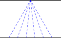
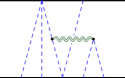
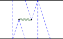
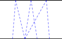
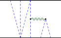
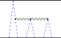
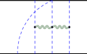
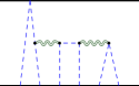
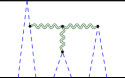
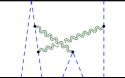
Figure 1: Sample diagrams for the $2\rightarrow 2$ scattering process in the static limit at 5PN order.

Diagrams that factorise when cutting an arbitrary number of worldlines correspond to multiple potential interactions and therefore yield no additional information. We discard such diagrams (column 3). Furthermore, the contributing graphs should not have loops out of world lines (column 4) and not contain massless tadpoles in the static limit (column 5).

Figure 2: The topologies contributing to the potential in the static limit at 5PN order.

At 5PN order 27582 diagrams remain. In principle, these can be reduced to a smaller set of diagrams by using symmetry relations under the exchange of the world lines and all vertices on each world line, introducing additional symmetry factors. This procedure would lead to the number of diagrams shown in column 6. Up to 4PN order, we have checked that those diagrams agree with those listed in [39, 45]. However, we find that this last symmetrisation provides no benefit in our setup and do not apply it in our calculation.

In the static limit the diagrams for $2\to 2$ scattering can be transformed into massless propagator-type diagrams representing the spacial potential between the two sources. At five-loop order we identify 22 top-level topologies, see Figure 2. We then insert the Feynman rules and perform algebraic simplifications using FORM [107, 108]. The remaining integrals are reduced using integration by parts [109] implemented in the package Crusher [110] leading to eight master integrals, out of which four contribute. In the same way we have calculated all the lower orders including 4PN. In the last column of Table 1 we list the number of master integrals, which turn out to be remarkably small. The present problem is by far simpler than the calculation of the five-loop $\beta$-function in QCD [111] and massive three-loop calculations in QCD, cf. [112].

	QGRAF	non fact.	no WL loops	no tadpoles	# Diag. [39]	# MI
N	1	1	1	1	1	-
1PN	2	2	2	2	1	1
2PN	19	19	19	15	5	1
3PN	360	276	258	122	8	1(1)
4PN	10081	5407	4685	1815	50	6(1)
5PN	332020	128080	101570	27582	154	4(4)

Table 1: Numbers of contributing diagrams at the different (post)-Newtonian levels and master integrals. The numbers in brackets denote the number of master integrals which occur during the reduction but do not contribute to the potential. In the next-to-last column the number of diagrams of equal value are given according to [39].

We have first calculated the static corrections up to 4PN in the way described above. The massless master integrals needed are known up to three loop order from Ref. [113] and at four loop order [114, 45, 46]. The master integrals depend on (multiple) zeta values [115], including $\ln(2)$. They have been compared to the numerical results given by FIESTA [116, 117, 118, 119]. Here it is useful to use the Monte Carlo integrator Divonne [120] of the CUBA package [121] besides VEGAS [122].

Figure 3: The master integral $M_{36}$ contributing to the 4th post-Newtonian approximation.

$M_{61}$	$M_{72}$	$M_{74}$	$M_{91}$

Figure 4: The five-loop master integrals contributing to the 5th post-Newtonian approximation in the static limit.

We use the $\overline{\sf MS}$-prescription in $d$ dimensions. The one-loop two-point function is therefore defined as

$$\vbox{\hbox{\includegraphics[width=45.0pt]{M21}}}=\int\frac{d^{d}k}{\pi^{d/2}}\frac{1}{((p-k)^{2})^{a}}\frac{1}{(k^{2})^{b}}=\frac{1}{(p^{2})^{a+b-d/2}}\frac{\Gamma\left(\frac{d}{2}-a\right)\Gamma\left(\frac{d}{2}-b\right)\Gamma\left(a+b-\frac{d}{2}\right)}{\Gamma(a)\Gamma(b)\Gamma\left(d-a-b\right)}\,.$$ (26)

The contributing five loop master integrals can all be traced back to lower loop structures by identifying effective propagator insertions. This leads to relations of the form

$$M(p^{2})=\int\frac{d^{d}k}{\pi^{d/2}}M_{1}\big{(}k^{2}\big{)}M_{2}\big{(}(p-k)^{2}\big{)}\,,$$ (27)

where $M_{1},M_{2}$ are suitably chosen propagator insertions and the argument of $M,M_{1},M_{2}$ denotes the respective external momentum squared. As a shorthand notation we define $M:=M(1)$ and $S_{\varepsilon}=\exp(-\gamma_{E}\varepsilon)$.

The most complicated insertion is

$$M_{36} = 2\pi^{2}S_{\varepsilon}^{4}\Biggl{[}\frac{1}{\varepsilon^{2}}+\frac{2}{\varepsilon}-2(16-\zeta_{2})+16\Biggl{[}9-6\zeta_{2}\left(\frac{13}{8}-\ln(2)\right)-\frac{77}{6}\zeta_{3}\Biggr{]}\Biggr{]}\varepsilon+O(\varepsilon^{2}),$$ (28)

cf. [45, 46]. A closed form representation for general values of $d$ of $M_{36}$ is not known. Here $\zeta_{k}=\sum_{l=1}^{\infty}(1/l^{k}),\leavevmode\nobreak\ \leavevmode\nobreak\ k\in\mathbb{N},\leavevmode\nobreak\ \leavevmode\nobreak\ k\geq 2$, denote Riemann’s $\zeta$-function at integers. With this, diagram $M_{91}$ can be obtained as a bubble insertion of diagram $M_{36}$ into the two-point function using

$$M_{91}(p^{2})=\int\frac{d^{d}k}{\pi^{d/2}}\frac{1}{((p-k)^{2})^{a}}\frac{M_{36}}{(k^{2})^{b}}=\frac{1}{(p^{2})^{a+b-d/2}}\frac{\Gamma\left(\frac{d}{2}-a\right)\Gamma\left(\frac{d}{2}-b\right)\Gamma\left(a+b-\frac{d}{2}\right)}{\Gamma(a)\Gamma(b)\Gamma\left(d-a-b\right)}M_{36},$$ (29)

where $a=1$ and $b=2+4\varepsilon$.

The results for all master integrals contributing to the potential read

$$M_{61} = \frac{\Gamma\left(6-\frac{5d}{2}\right)\Gamma^{6}\left(-1+\frac{d}{2}\right)}{\Gamma(-6+3d)}$$

$$= S_{\varepsilon}^{5}\pi^{7/2}\Biggl{[}\frac{2}{3}+\left(\frac{134}{9}+\frac{4}{3}\ln(2)\right)\varepsilon+\left(\frac{5894}{27}+\frac{268}{9}\ln(2)+\frac{4}{3}\ln^{2}(2)+19\zeta_{2}\right)\varepsilon^{2}\Biggr{]}+O(\varepsilon^{3})\,,$$

$$M_{72} = \frac{\Gamma\left(7-\frac{5d}{2}\right)\Gamma\left(3-d\right)\Gamma\left(2-\frac{d}{2}\right)\Gamma^{7}\left(-1+\frac{d}{2}\right)\Gamma(2d-5)}{\Gamma\left(5-\frac{3}{2}d\right)\Gamma(-2+d)\Gamma\left(-3+\frac{3}{2}d\right)\Gamma\left(-7+3d\right)}$$ (31)

$$= -S_{\varepsilon}^{5}\pi^{7/2}\Biggl{[}\frac{2}{\varepsilon}+4\left(11+\ln(2)\right)+\left(656+88\ln(2)+4\ln^{2}(2)+25\zeta_{2}\right)\varepsilon$$

$$+\left(8288+1312\ln(2)+88\ln^{2}(2)+550\zeta_{2}+\frac{8}{3}\ln^{3}(2)+50\ln(2)\zeta_{2}-\frac{2002}{3}\zeta_{3}\right)\varepsilon^{2}\Biggr{]}$$

$$+O(\varepsilon^{3})\,,$$

$$M_{74} = \frac{\Gamma\left(7-\frac{5d}{2}\right)\Gamma^{2}(3-d)\Gamma^{7}\left(-1+\frac{d}{2}\right)\Gamma\left(-6+\frac{5d}{2}\right)}{\Gamma\left(6-2d\right)\Gamma^{2}\left(-3+\frac{3d}{2}\right)\Gamma\left(-7+3d\right)}$$ (32)

$$= -S_{\varepsilon}^{5}\pi^{7/2}\Biggl{[}\frac{4}{\varepsilon}+72+8\ln(2)+\left(864+144\ln(2)+8\ln^{2}(2)+146\zeta_{2}\right)\varepsilon$$

$$+\left(8640+1728\ln(2)+144\ln^{2}(2)+2628\zeta_{2}+\frac{16}{3}\ln^{3}(2)+292\zeta_{2}\ln(2)-\frac{1988}{3}\zeta_{3}\right)\varepsilon^{2}\Biggr{]}$$

$$+O(\varepsilon^{3})\,,$$

$$M_{91} = 6\pi^{7/2}S_{\varepsilon}^{5}\Biggl{[}\frac{2}{\varepsilon}-4(1-\ln(2))-\left(48+8\ln(2)-4\ln^{2}(2)-105\zeta_{2}\right)\varepsilon+\Biggl{(}480-96\ln(2)$$ (33)

$$-8\ln^{2}(2)+\frac{8}{3}\ln^{3}(2)-530\zeta_{2}+402\ln(2)\zeta_{2}-\frac{1522}{3}\zeta_{3}\Biggr{)}\varepsilon^{2}\Biggr{]}+O(\varepsilon^{3})\,.$$

4 Results

Inserting the master integrals into the expression for the static contribution to the Lagrangian it turns out that all pole contributions in the dimensional parameter $\varepsilon$ cancel.

$${\cal L}^{S}={\cal L}_{N}^{S}+{\cal L}_{PN_{1}}^{S}+{\cal L}_{PN_{2}}^{S}+{\cal L}_{PN_{3}}^{S}+{\cal L}_{PN_{4}}^{S}+{\cal L}_{PN_{5}}^{S}$$ (34)

up to the fifth post-Newtonian order. One obtains the following contributions to the static Lagrangian up to the 5th PN order:

$${\cal L}_{N}^{S} =\frac{G_{N}}{r}m_{1}m_{2},$$ [71] (35)

$${\cal L}_{PN_{1}}^{S} =-\frac{G_{N}^{2}}{2r^{2}}m_{1}m_{2}(m_{1}+m_{2}),$$ [16] (36)

$${\cal L}_{PN_{2}}^{S} =\frac{G_{N}^{3}}{r^{3}}m_{1}m_{2}\left(\frac{1}{2}(m_{1}^{2}+m_{2}^{2})+3m_{1}m_{2}\right),$$ [34] (37)

$${\cal L}_{PN_{3}}^{S} =-\frac{G_{N}^{4}}{r^{4}}m_{1}m_{2}\left[\frac{3}{8}\left(m_{1}^{3}+m_{2}^{3}\right)+6m_{1}m_{2}(m_{1}+m_{2})\right],$$ [37] (38)

$${\cal L}_{PN_{4}}^{S} =\frac{G_{N}^{5}}{r^{5}}m_{1}m_{2}\left[\frac{3}{8}\left(m_{1}^{4}+m_{2}^{4}\right)+\frac{31}{3}m_{1}m_{2}\left(m_{1}^{2}+m_{2}^{2}\right)+\frac{141}{4}m_{1}^{2}m_{2}^{2}\right],$$ [45] (39)

$${\cal L}_{PN_{5}}^{S} =-\frac{G_{N}^{6}}{r^{6}}m_{1}m_{2}\Biggl{[}\frac{5}{16}(m_{1}^{5}+m_{2}^{5})+\frac{91}{6}m_{1}m_{2}(m_{1}^{3}+m_{2}^{3})+\frac{653}{6}m_{1}^{2}m_{2}^{2}(m_{1}+m_{2})\Biggr{]},$$ (40)

with $r=|{\bf r}_{1}-{\bf r}_{2}|$. We agree with the above results in the literature up to ${\cal L}_{PN_{4}}^{S}$. Moreover, including 5PN, all the contributions due to multiple zeta values also cancel and only rational coefficients remain.

To be explicit, the pole part of ${\cal L}_{PN_{5}}^{S}$ in terms of the master integrals is given by

$$\Big{[}{\cal L}_{PN_{5}}^{S}\Big{]}_{\varepsilon^{-1}}=\frac{G_{N}^{6}}{r^{6}}(m_{1}m_{2})^{3}(m_{1}+m_{2})\pi^{-7/2}\frac{45}{32}\Big{[}2M_{72}-M_{74}\Big{]}_{\varepsilon^{-1}}=0\,,$$ (41)

where $[X]_{\varepsilon^{n}}$ denotes the coefficient of $\varepsilon^{n}$ in $X$. With this in mind, the finite part can be written as

$$\begin{split}\Big{[}{\cal L}_{PN_{5}}^{S}\Big{]}_{\varepsilon^{0}}={}&-\frac{G_{N}^{6}}{r^{6}}(m_{1}m_{2})\pi^{-7/2}\left\{\frac{15}{32}(m_{1}^{5}+m_{2}^{5})\Big{[}M_{61}\Big{]}_{\varepsilon^{0}}+\frac{91}{4}m_{1}m_{2}(m_{1}^{3}+m_{2}^{3})\Big{[}M_{61}\Big{]}_{\varepsilon^{0}}\right.\\ &\quad+m_{1}^{2}m_{2}^{2}(m_{1}+m_{2})\left(\Big{[}\frac{293}{4}M_{61}-\frac{45}{16}M_{72}+\frac{45}{32}M_{74}\Big{]}_{\varepsilon^{0}}\right.\\ &\left.\left.\qquad+\Big{[}\frac{519}{16}M_{72}-\frac{627}{32}M_{74}+2M_{91}\Big{]}_{\varepsilon^{-1}}\right)\right\}\,.\end{split}$$ (42)

We remark that up to the term ${\cal L}_{PN_{1}}$ the results also agree to the zero–velocity limit of [42, 40]. In the limit $m_{1}\ll m_{2}$ the coefficients of the leading terms of $O(m_{1}(G_{N}m_{2}/r)^{k})$ for $k\in\mathbb{N},\leavevmode\nobreak\ k\geq 1$ are obtained as the expansion coefficients of the generating function $-m_{1}[\sqrt{(1-x)/(1+x)}|_{x=G_{N}m_{2}/r}-1]$ in accordance with the Schwarzschild solution of a test particle in the field of a second mass.

5 Conclusions

We have calculated the five-loop correction to the gravitational interaction potential between two static point masses. This constitutes an important part of the effective gravitational Lagrangian at fifth post-Newtonian order. We also agree with the corresponding results in the lower post-Newtonian orders. The calculation of the velocity-dependent terms at this order is work in progress.

Acknowledgments

We would like to thank Prof. Th. Damour and Prof. G. Schäfer for very helpful comments and P. Nogueira for a discussion. This project has received funding from the European Union’s Horizon 2020 research and innovation programme under the Marie Sklodowska-Curie grant agreement No. 764850, SAGEX, and COST action CA16201: Unraveling new physics at the LHC through the precision frontier.

Note added.
A few hours before the present submission the preprint [123] appeared, presenting an independent calculation of the same quantity. The final results, Eq. (40) in this work and Eq. (32) in [123], are in agreement.

References

- [1] B.P. Abbott et al. [LIGO Scientific and Virgo Collaborations], Phys. Rev. Lett. 116 (2016) no. 6, 061102 [arXiv:1602.03837 [gr-qc]]; Phys. Rev. Lett. 119, no. 16, 161101 (2017) [arXiv:1710.05832 [gr-qc]].
- [2] https://en.wikipedia.org/wiki/Gravitational-wave_observatory
- [3] A. Buonanno and T. Damour, Phys. Rev. D 59 (1999) 084006 [gr-qc/9811091].
- [4] A. Buonanno and T. Damour, Phys. Rev. D 62 (2000) 064015 [gr-qc/0001013].
- [5] T. Damour, F. Guercilena, I. Hinder, S. Hopper, A. Nagar and L. Rezzolla, Phys. Rev. D 89 (2014) no. 8, 081503 [arXiv:1402.7307 [gr-qc]].
- [6] T. Damour, Phys. Rev. D 94 (2016) no. 10, 104015 [arXiv:1609.00354 [gr-qc]].
- [7] T. Damour, Phys. Rev. D 97 (2018) no. 4, 044038 [arXiv:1710.10599 [gr-qc]].
- [8] J. Vines, Class. Quant. Grav. 35 (2018) no. 8, 084002 [arXiv:1709.06016 [gr-qc]].
- [9] F. Pretorius, Phys. Rev. Lett. 95 (2005) 121101 [gr-qc/0507014].
- [10] M. Campanelli, C.O. Lousto, P. Marronetti and Y. Zlochower, Phys. Rev. Lett. 96 (2006) 111101 [gr-qc/0511048].
- [11] J.G. Baker, J. Centrella, D.I. Choi, M. Koppitz and J. van Meter, Phys. Rev. Lett. 96 (2006) 111102 [gr-qc/0511103].
- [12] Y. Mino, M. Sasaki and T. Tanaka, Phys. Rev. D 55 (1997) 3457–3476 [gr-qc/9606018].
- [13] T.C. Quinn and R.M. Wald, Phys. Rev. D 56 (1997) 3381–3394 [gr-qc/9610053].
- [14] A. Einstein, Sitzungsber. Preuss. Akad. Wiss. (1915) 831–839.
-
[15]
J. Droste,
Proc. Acad. Sci. Amst. 19 (1916) 447–455;
H. Lorentz and J. Droste, in: The motion of a system of bodies under the influence of their mutual attraction, according to Einstein’s theory, (Nijhoff, The Hague, 1937) pp. 330–355. - [16] A. Einstein, L. Infeld and B. Hoffmann, Annals Math. 39 (1938) 65–100.
- [17] V. Fock, J. Phys. (Moscow) 1 (1939) 81–116; Theory of Space, Time and Gravitation, (Pergamon, London, 1959).
- [18] J.F. Plebański and S.L. Bażański, Acta Phys. Pol. 18 (1959) 307–345.
-
[19]
S. Chandrasekhar,
Astrophys. J. 142 (1965) 1488-1512;
Astrophys. J. 158 (1969) 45–54;
S. Chandrasekhar and Y. Nutku, Astrophys. J. 158 (1969) 55–79;
S. Chandrasekhar and F. Esposito, Astrophys. J. 160 (1970) 153–179. - [20] T. Kimura and T. Toiya, Prog. Theor. Phys. 48 (1972) 316–328.
- [21] T. Ohta, H. Okamura, T. Kimura and K. Hiida, Prog. Theor. Phys. 50 (1973) 492–514; 51 (1974) 1220–1238.
- [22] T. Ohta, H. Okamura, T. Kimura and K. Hiida, Prog. Theor. Phys. 51 (1974) 1598–1612.
- [23] T. Damour and G. Schäfer, Gen. Rel. Grav. 17 (1985) 879–905.
- [24] L. Blanchet and T. Damour, Phys. Rev. D 37 (1988) 1410–1435.
- [25] N. Wex and G. Schäfer, Phys. Lett. A 174 (1993) 196–205.
- [26] P. Jaranowski and G. Schäfer, Phys. Rev. D 57 (1998) 7274–7291 Erratum: [Phys. Rev. D 63 (2001) 029902] [gr-qc/9712075].
- [27] T. Damour, P. Jaranowski and G. Schäfer, Phys. Rev. D 62 (2000) 044024 [gr-qc/9912092]
- [28] L. Blanchet and G. Faye, Phys. Lett. A 271 (2000) 58–64 [gr-qc/0004009].
- [29] V.C. de Andrade, L. Blanchet and G. Faye, Class. Quant. Grav. 18 (2001) 753–778 [gr-qc/0011063].
- [30] T. Damour, P. Jaranowski and G. Schäfer, Phys. Lett. B 513 (2001) 147–155 [gr-qc/0105038].
- [31] T. Damour, P. Jaranowski and G. Schäfer, Phys. Rev. D 62 (2000) 021501 Erratum: [Phys. Rev. D 63 (2001) 029903] [gr-qc/0003051].
- [32] N.E.J. Bjerrum-Bohr, J.F. Donoghue and B.R. Holstein, Phys. Rev. D 67 (2003) 084033 Erratum: [Phys. Rev. D 71 (2005) 069903] [hep-th/0211072].
- [33] B. Kol and M. Smolkin, Class. Quant. Grav. 25 (2008) 145011 [arXiv:0712.4116 [hep-th]].
- [34] J.B. Gilmore and A. Ross, Phys. Rev. D 78 (2008) 124021 [arXiv:0810.1328 [gr-qc]].
- [35] B. Kol, M. Levi and M. Smolkin, Class. Quant. Grav. 28 (2011) 145021 [arXiv:1011.6024 [gr-qc]].
- [36] B. Kol and M. Smolkin, Phys. Rev. D 85 (2012) 044029 [arXiv:1009.1876 [hep-th]].
- [37] S. Foffa and R. Sturani, Phys. Rev. D 84 (2011) 044031 [arXiv:1104.1122 [gr-qc]].
- [38] D. Bini and T. Damour, Phys. Rev. D 87 (2013) no.12, 121501 doi:10.1103/PhysRevD.87.121501 [arXiv:1305.4884 [gr-qc]].
- [39] S. Foffa and R. Sturani, Phys. Rev. D 87 (2013) no.6, 064011 [arXiv:1206.7087 [gr-qc]].
- [40] T. Damour, P. Jaranowski and G. Schäfer, Phys. Rev. D 89 (2014) no. 6, 064058 [arXiv:1401.4548 [gr-qc]].
- [41] P. Jaranowski and G. Schäfer, Phys. Rev. D 92 (2015) no. 12, 124043 [arXiv:1508.01016 [gr-qc]];
- [42] L. Bernard, L. Blanchet, A. Bohé, G. Faye and S. Marsat, Phys. Rev. D 93 (2016) no.8, 084037 [arXiv:1512.02876 [gr-qc]].
- [43] T. Damour, P. Jaranowski and G. Schäfer, Phys. Rev. D 93 (2016) no.8, 084014 [arXiv:1601.01283 [gr-qc]].
- [44] L. Bernard, L. Blanchet, A. Bohé, G. Faye and S. Marsat, Phys. Rev. D 95 (2017) no.4, 044026 doi:10.1103/PhysRevD.95.044026 [arXiv:1610.07934 [gr-qc]].
- [45] S. Foffa, P. Mastrolia, R. Sturani and C. Sturm, Phys. Rev. D 95 (2017) no.10, 104009 [arXiv:1612.00482 [gr-qc]].
- [46] T. Damour and P. Jaranowski, Phys. Rev. D 95 (2017) no.8, 084005 [arXiv:1701.02645 [gr-qc]].
- [47] D. Bini and T. Damour, Phys. Rev. D 96 (2017) no. 6, 064021 [arXiv:1706.06877 [gr-qc]].
- [48] N.E.J. Bjerrum-Bohr, P.H. Damgaard, G. Festuccia, L. Planté and P. Vanhove, Phys. Rev. Lett. 121 (2018) no. 17, 171601 [arXiv:1806.04920 [hep-th]].
- [49] J. Plefka, J. Steinhoff and W. Wormsbecher, Phys. Rev. D 99 (2019) no.2, 024021 [arXiv:1807.09859 [hep-th]].
- [50] D.A. Kosower, B. Maybee and D. O’Connell, Amplitudes, Observables, and Classical Scattering, arXiv:1811.10950 [hep-th].
- [51] A. Antonelli, A. Buonanno, J. Steinhoff, M. van de Meent and J. Vines, Energetics of two-body Hamiltonians in post-Minkowskian gravity, arXiv:1901.07102 [gr-qc].
- [52] B. Bertotti, Nuovo Cimento 4 (1956) 898–906.
- [53] R.P. Kerr, Nuovo Cimento 13 (1959) 469–491.
- [54] B. Bertotti, J.F. Plebański, Ann. Phys. 11 (1960) 169–200.
- [55] M. Portilla, J. Phys. A 12, 1075 (1979) 1075–1090.
- [56] K. Westpfahl and M. Goller, Lett. Nuovo Cim. 26 (1979) 573–576.
- [57] M. Portilla, J. Phys. A 13 (1980) 3677–3683.
- [58] L. Bel, T. Damour, N. Deruelle, J. Ibanez and J. Martin, Gen. Rel. Grav. 13 (1981) 963–1004.
- [59] K. Westpfahl, Fortschr. Phys., 33 (1985) 417–493.
- [60] S. Foffa, Phys. Rev. D 89 (2014) no.2, 024019 [arXiv:1309.3956 [gr-qc]].
- [61] C. Cheung, I.Z. Rothstein and M.P. Solon, Phys. Rev. Lett. 121 (2018) no. 25, 251101 [arXiv:1808.02489 [hep-th]].
- [62] Z. Bern, C. Cheung, R. Roiban, C.H. Shen, M.P. Solon and M. Zeng, Scattering Amplitudes and the Conservative Hamiltonian for Binary Systems at Third Post-Minkowskian Order, arXiv:1901.04424 [hep-th].
- [63] T. Damour and G. Esposito-Farese, Phys. Rev. D 53 (1996) 5541–5578 [gr-qc/9506063].
- [64] W.D. Goldberger and I.Z. Rothstein, Phys. Rev. D 73 (2006) 104029 [hep-th/0409156].
- [65] T. Futamase and Y. Itoh, Living Rev. Rel. 10 (2007) 2–81.
- [66] L. Blanchet, Living Rev. Rel. 17 (2014) 2–187 [arXiv:1310.1528 [gr-qc]].
- [67] R.A. Porto, Phys. Rept. 633 (2016) 1–104 [arXiv:1601.04914 [hep-th]].
- [68] G. Schäfer and P. Jaranowski, Living Rev. Rel. 21, no. 1 (2018) 1–118 [arXiv:1805.07240 [gr-qc]].
- [69] L. Barack and A. Pound, Rept. Prog. Phys. 82, no. 1 (2019) 016904 [arXiv:1805.10385 [gr-qc]].
- [70] M. Levi, Effective field theories of post-Newtonian gravity: A comprehensive review, arXiv:1807.01699 [hep-th], 70 p.
- [71] I. Newton, Philosophiae Naturalis Principia Mathematica, (S. Pepys, Londini, 1686); German translation by J. Ph. Wolfers, (R. Oppenheim, Berlin 1872).
- [72] G. Schäfer, Annals Phys. 161 (1985) 81–100.
- [73] P. Jaranowski and G. Schäfer, Phys. Rev. D 55 (1997) 4712–4722.
- [74] A. Luna, R. Monteiro, I. Nicholson, D. O’Connell and C.D. White, JHEP 1606 (2016) 023 [arXiv:1603.05737 [hep-th]].
- [75] W.D. Goldberger and A.K. Ridgway, Phys. Rev. D 95 (2017) no. 12, 125010 [arXiv:1611.03493 [hep-th]].
- [76] W.D. Goldberger, S.G. Prabhu and J.O. Thompson, Phys. Rev. D 96 (2017) no. 6, (2017) 065009 [arXiv:1705.09263 [hep-th]].
- [77] W.D. Goldberger and A.K. Ridgway, Phys. Rev. D 97 (2018) no. 8, 085019 [arXiv:1711.09493 [hep-th]].
- [78] D. Chester, Phys. Rev. D 97 (2018) no. 8, 084025 [arXiv:1712.08684 [hep-th]].
- [79] W.D. Goldberger, J. Li and S.G. Prabhu, Phys. Rev. D 97 (2018) no. 10, 105018 [arXiv:1712.09250 [hep-th]].
- [80] J. Li and S.G. Prabhu, Phys. Rev. D 97 (2018) no. 10, 105019 [arXiv:1803.02405 [hep-th]].
- [81] C.H. Shen, JHEP 1811 (2018) 162 [arXiv:1806.07388 [hep-th]].
- [82] G. Faye, L. Blanchet, and A. Buonanno, Phys. Rev. D 74 (2006) [Errata: Phys. Rev. D 75 (2007) 049903; Phys. Rev. D 81 (2010) 089901].
- [83] R. Porto and I. Rothstein, Phys.Rev.Lett. 97 (2006) 021101; Phys. Rev. D 78 (2008) 044012 [Errata: Phys. Rev. D 81 (2010) 029904; Phys. Rev. D 81 (2010) 029905]; Phys. Rev. D 78 (2008) 044013 [Errata: Phys. Rev. D 81 (2010) 029904; Phys. Rev. D 81 (2010) 029905].
- [84] J. Steinhoff, S. Hergt, and Gerhard Schf̈er, Phys. Rev. D 7 (2008) 081501(R); Phys. Rev. D 78 (2008) 101503(R).
- [85] B.R. Holstein and A. Ross, arXiv:0802.0716 [hep-ph].
- [86] M. Levi, Phys. Rev. D 82 (2010) 104004; Phys. Rev. D 82 (2010) 064029; Phys. Rev. D 85 (2012) 064043 [arXiv:1107.4322 [gr-qc]].
- [87] R. Porto, Class. Quant. Grav. 27 (2010) 205001.
- [88] J. Steinhoff, Ann. Phys. (Leipzig) 523 (2011) 296–353.
- [89] J. Hartung and J. Steinhoff, Ann. Phys. (Leipzig) 523 (2011) 783–790.
- [90] J. Hartung, J. Steinhoff, and G. Schäfer, Ann. Phys. (Leipzig) 525 (2013) 359–394.
- [91] A. Bohé, S. Marsat, and L. Blanchet, Class. Quant. Grav. 30 (2013) 135009
- [92] A. Bohé, G. Faye, S. Marsat, and E.K. Porter, Class. Quant. Grav. 32 (2015) no.19, 195010
- [93] V. Vaidya, Phys. Rev. D 91 (2015) no. 2, 024017 [arXiv:1410.5348 [hep-th]].
- [94] M. Levi and J. Steinhoff, JCAP 1601 (2016) 008 [arXiv:1506.05794 [gr-qc]].
- [95] M. Levi and J. Steinhoff, JHEP 1509 (2015) 219 [arXiv:1501.04956 [gr-qc]].
- [96] A. Guevara, Holomorphic classical limit for spin efffects in gravitational and electromagnetic scattering, arXiv:1706.02314 [hep-th].
- [97] A. Guevara, A. Ochirov and J. Vines, Scattering of spinning black holes from exponentiated soft factors, arXiv:1812.06895 [hep-th].
- [98] M.Z. Chung, Y.T. Huang, J.W. Kim and S. Lee, The simplest massive S-matrix: from minimal coupling to Black Holes, arXiv:1812.08752 [hep-th].
-
[99]
T. Kaluza,
Sitzungsber. Preuss. Akad. Wiss. Berlin (Math. Phys. ) 1921 (1921) 966–972
[arXiv:1803.08616 [physics.hist-ph]];
O. Klein, Z. Phys. 37 (1926) 895–906 [Surveys High Energ. Phys. 5 (1986) 241–244]. - [100] H. Weyl, Raum, Zeit, Materie, (Springer, Berlin, 1918).
-
[101]
R. Clausius, Ann. Phys. (Leipzig) 217 (1870) 124–130;
H. Stephani and G. Kluge, Einführung in die theoretische Mechanik (DVW, Berlin, 1975). - [102] L. Blanchet, T. Damour and G. Esposito-Farese, Phys. Rev. D 69 (2004) 124007 [gr-qc/0311052].
- [103] M. Levi and J. Steinhoff, Class. Quant. Grav. 34 (2017) no.24, 244001 [arXiv:1705.06309 [gr-qc]].
- [104] P. Nogueira, J. Comput. Phys. 105 (1993) 279–289.
-
[105]
A.V. Smirnov, V.A. Smirnov and M. Steinhauser,
Phys. Lett. B 668 (2008) 293–298
[arXiv:0809.1927 [hep-ph]];
R.N. Lee, A.V. Smirnov, V.A. Smirnov and M. Steinhauser, Phys. Rev. D 94 (2016) no.5, 054029 [arXiv:1608.02603 [hep-ph]]. - [106] C. Anzai, Y. Kiyo and Y. Sumino, Phys. Rev. Lett. 104 (2010) 112003 [arXiv:0911.4335 [hep-ph]].
- [107] J.A.M. Vermaseren, New features of FORM, math-ph/0010025.
- [108] M. Tentyukov and J.A.M. Vermaseren, Comput. Phys. Commun. 181 (2010) 1419–1427 [hep-ph/0702279].
-
[109]
J. Lagrange, Nouvelles recherches sur la nature et la propagation du son,
Miscellanea Taurinensis t. II (1760-61) 263;
C.F. Gauß, Theoria attractionis corporum sphaeroidicorum ellipticorum homogeneorum methodo novo tractate, Commentationes societas scientiarum Gottingensis recentiores III (1813) 5–7;
G. Green, Essay on the mathematical theory of electricity and magnetism, Nottingham (1828), Green Papers, pp. 1–115;
M. Ostrogradski, Mem. Ac. Sci. St. Peters. 6 (1831) 129–133;
K.G. Chetyrkin and F.V. Tkachov, Nucl. Phys. B 192 (1981) 159–204;
S. Laporta, Int. J. Mod. Phys. A 15 (2000) 5087–5159 [hep-ph/0102033]. - [110] P. Marquard and D. Seidel, The package Crusher, (unpublished).
-
[111]
P.A. Baikov, K.G. Chetyrkin and J.H. Kühn,
Phys. Rev. Lett. 118 (2017) no.8, 082002
[arXiv:1606.08659 [hep-ph]];
F. Herzog, B. Ruijl, T. Ueda, J.A.M. Vermaseren and A. Vogt, JHEP 1702 (2017) 090 [arXiv:1701.01404 [hep-ph]];
T. Luthe, A. Maier, P. Marquard and Y. Schröder, JHEP 1710 (2017) 166 [arXiv:1709.07718 [hep-ph]];
K.G. Chetyrkin, G. Falcioni, F. Herzog and J.A.M. Vermaseren, JHEP 1710 (2017) 179 Addendum: [JHEP 1712 (2017) 006] [arXiv:1709.08541 [hep-ph]]. -
[112]
R.N. Lee, A.V. Smirnov, V.A. Smirnov and M. Steinhauser,
JHEP 1805 (2018) 187
[arXiv:1804.07310 [hep-ph]];
J. Ablinger, J. Blümlein, P. Marquard, N. Rana and C. Schneider, Nucl. Phys. B 939 (2019) 253–291 [arXiv:1810.12261 [hep-ph]];
J. Ablinger, A. Behring, J. Blümlein, A. De Freitas, A. von Manteuffel and C. Schneider, Nucl. Phys. B 890 (2014) 48–151 [arXiv:1409.1135 [hep-ph]]; PoS QCDEV 2017 (2017) 031 [arXiv:1711.07957 [hep-ph]]. - [113] K.G. Chetyrkin, A.L. Kataev and F.V. Tkachov, Nucl. Phys. B 174 (1980) 345–377.
- [114] P.A. Baikov and K.G. Chetyrkin, Nucl. Phys. B 837 (2010) 186 [arXiv:1004.1153 [hep-ph]].
- [115] J. Blümlein, D.J. Broadhurst and J.A.M. Vermaseren, Comput. Phys. Commun. 181 (2010) 582–625 [arXiv:0907.2557 [math-ph]].
- [116] T. Binoth and G. Heinrich, Nucl. Phys. B 680 (2004) 375–388 [hep-ph/0305234].
- [117] A.V. Smirnov and M.N. Tentyukov, Comput. Phys. Commun. 180 (2009) 735–746 [arXiv:0807.4129 [hep-ph]].
- [118] A.V. Smirnov, V.A. Smirnov and M. Tentyukov, Comput. Phys. Commun. 182 (2011) 790–803 [arXiv:0912.0158 [hep-ph]].
- [119] A.V. Smirnov, Comput. Phys. Commun. 204 (2016) 189–199 [arXiv:1511.03614 [hep-ph]].
- [120] J.H. Friedman, M.H. Wright, ACM Trans. Math. Software 7 (1981) 76–92; CGTM-193-REV, CGTM-193.
- [121] T. Hahn, Comput. Phys. Commun. 168 (2005) 78–95 [hep-ph/0404043].
- [122] G.P. Lepage, J. Comput. Phys. 27 (1978) 192–203; Vegas: An Adaptive Multidimensional Integration Program, CLNS-80/447.
- [123] S. Foffa, P. Mastrolia, R. Sturani, C. Sturm and W. J. Torres Bobadilla, Static two-body potential at fifth post-Newtonian order, arXiv:1902.10571 [gr-qc].