Abstract

We calculate the motion of binary mass systems in gravity up to the fourth post–Newtonian order. We use momentum expansions within an effective field theory approach based on Feynman amplitudes in harmonic coordinates by applying dimensional regularization. We construct the canonical transformations to ADM coordinates and to effective one body theory (EOB) to compare with other approaches. We show that intermediate poles in the dimensional regularization parameter $\varepsilon$ vanish in the observables and the classical theory is not renormalized. The results are illustrated for a series of observables for which we agree with the literature.

1 Introduction

Precise predictions for observables describing the merging of two heavy astrophysical objects like black holes or neutron stars are very important [1]. In particular the spiral-in phase of these processes can be described by analytic calculations. Methods of non-relativistic effective field theory [3, 2, 4, 5, 8, 9, 6, 7] allow to calculate the equations of motion of a binary mass system within the post–Newtonian (PN) approach. We will limit ourselves to the non-spinning case in the following. Until now the corrections have been computed to the 4th post–Newtonian order [2, 4, 5, 8, 9]. There are first corrections due to the static potential at 5PN [6, 7], see also [10]. The corrections up to 4PN were derived by using other methods, cf.  Refs. [11, 12], before. Very recently first partial results up to the 5th post–Newtonian order have been obtained in [13]. In the post–Newtonian approach one retains all terms in the velocity being of the same order as the pure potential terms by the virial theorem [14]. Recently also important progress has been made in the post-Minkowskian (PM) approach reaching 3PM cf. [15, 16], see also [17].

In this paper we present the corrections up to 4PN obtained using effective field theory methods. Here we apply dimensional regularization in calculating the Feynman integrals. At intermediary steps the dimensional parameter $D=4-2\varepsilon$ occurs. We perform multiple comparisons to results in the literature and find agreement. Starting at 3PN singular contributions of $O(1/\varepsilon)$ occur when working in harmonic coordinates. From 4PN onward singularities of $O(1/\varepsilon)$ also result from the tail terms, cf. also [5, 8]. By applying canonical transformations one may map the Hamiltonian in harmonic coordinates into a class of pole–free Hamiltonians at 3PN, to which the ADM and EOB Hamiltonians belong. This is also the case at 4PN when accounting for the tail terms before. Therefore, the classical observables are free of the intermediary regularization parameter.

The paper is organized as follows. In Section 2 we describe the calculation method. We outline the general framework and present the results up to 4PN in harmonic coordinates by deriving the effective Hamiltonian using the Hamiltonian formalism [18] in the center of momentum frame. The cancellation of the pole contributions is discussed. We also present an associated pole–free Hamiltonian obtained after applying a canonical transformation. At 3PN one also obtains a $\ln(r)$ free Hamiltonian, with $r=|\vec{x}_{1}-\vec{x}_{2}|$. In Section 3 we construct the canonical transformation to ADM coordinates, to compare with these results. In Section 4 we study the canonical transformation to EOB coordinates, which are widely used in the literature and present the EOB Hamiltonian up to 4PN in explicit form. We present numerical results for the energy of the innermost stable orbit and the angular momentum for circular coordinates in Section 5. Section 6 contains the conclusions. In an appendix we present the general $D$-dimensional Hamiltonian in harmonic coordinates up to $O(\varepsilon)$ in explicit form, which is also important for higher post–Newtonian calculations.

2 Calculation Method

2.1 The general framework

The main steps of our calculation have already been described in Ref. [7] calculating the static potential to 5PN ab initio. Now we add the different velocity contributions up to 4PN. Starting from the Einstein–Hilbert Lagrangian, one parameterizes the metric $g_{\mu\nu}$ as proposed in [2] in terms of one scalar, a three-component vector and a six-component tensor field. Within this parameterization one can derive the contributing Feynman rules using the path integral. The corresponding Feynman diagrams are generated using QGRAF [19], after providing the corresponding Feynman rules. We consider only the classical contributions and calculate the effective two–body potential. Here the necessary velocity contributions range up to $O((G_{N}\overline{M}/r)^{k}(v^{2})^{n-k+1})$, with $G_{N}$ Newton’s constant, $\overline{M}$ a mass scale, $r$ the distance of the point masses and $v\in\{v_{1},v_{2}\}$ their velocities. We will set $c=1$ in many places and keep it only when needed as an order parameter. The Lorentz algebra is carried out using Form [20] and the reduction to master integrals is performed using the code Crusher [21]. The contributing master integrals are known from the calculation of the static potential already, cf. [7] and references therein. One first obtains a Lagrange function of $m$th order containing also the accelerations $a_{i}$ and time derivatives thereof.

In Table 1 we give an overview on the complexity of the calculation up to 4PN and give the numbers of generated diagrams, the number of non factorizing diagrams, those with no world-line loops and no tadpoles by loop order. The initial number of 25324 diagrams reduces to 9266 contributing to the present result. Here we do not sort them in addition into equivalence classes and do thus determine the final combinatorial factors by the calculation itself.

	QGRAF	non fact.	no WL loops	no tadpoles	# Diag. [8, 22]	# MI
0	3	3	3	3	3	0
1	70	70	70	70	23	1
2	1770	1770	1770	1468	212	1
3	13400	9792	9482	5910	317	1
4	10081	5407	4685	1815	50	4(3)

Table 1: Numbers of contributing diagrams at the different loop levels and master integrals (MI). The numbers in brackets denote the number of master integrals which occur during the reduction but do not contribute to the potential. In the next-to-last column the number of diagrams of the respective equivalence classes are given according to [22, 8].

The computation time for the complete project from Feynman diagram generation, IBP reduction to the final results amounts to a few hours using an Intel(R) Core(TM) i7-8650U CPU.

The present results and those from [4, 22, 8] are given in form of an $m$th order Lagrange-density, from which one may derive the associated equation of motion [23]

$$\delta S=\int d^{D}x\left\{\sum_{k=0}^{m}(-1)^{k+1}\frac{d^{k}}{dt^{k}}\left[\frac{\partial{\cal L}}{\partial U_{\Omega|{\tiny\underbrace{t..t}_{k}}}}\right]\right\}\delta U_{\Omega}=0,$$ (1)

with ${\cal L}$ the Lagrangian density and $U_{\Omega}\in\{x_{1},x_{2}\}$, the coordinates of the two point masses and $U_{\Omega|t}=\partial_{t}U_{\Omega}$. The present results, although widely different in form and probably based on different Feynman rules, can be compared using the equation of motion (1) finding agreement with the corresponding equation of motion for the Lagrangians given in [4, 22, 8]. This applies to the potential contributions. In addition the tail terms have to be considered, cf. [8, 24, 33].

The next step is to eliminate the accelerations and their time derivatives. For this we use double zero insertions [25], up to linear terms in the acceleration. These are eliminated by a coordinate shift [26, 25, 27] implying the contribution of variational derivatives of the Lagrangian and a total time derivative. This procedure is applied to the $D$-dimensional Lagrangian for all post–Newtonian orders. The first order Lagrangian density is then obtained in somewhat different coordinates from harmonic coordinates [27]. Finally, we perform the Legendre transformation to obtain the Hamiltonian.

2.2 Remarks on the 4PN Tail Term

The quadrupole structure of the tail term at 4PN results from the leading term in the multipole expansion of the retarded radiation field from linearized Einstein gravity, cf. [28],

$$h^{\mu\nu}=|g|^{1/2}g^{\mu\nu}-\eta^{\mu\nu},$$ (2)

with $\eta^{\mu\nu}$ the Minkowski metric and $|g|$ the modulus of the determinant of the metric tensor. Let $L$ be the multi–index $L=i_{1},i_{2},...,i_{l}$, then the components of $h^{\mu\nu}$ are given by

$$h^{00} = -\frac{4G_{N}}{c^{2}}\sum_{l=0}^{\infty}\frac{(-1)^{l}}{l!}\partial_{L}\tilde{I}_{L},$$ (3)

$$h^{0i} = \frac{4G_{N}}{c^{3}}\sum_{l=1}^{\infty}\frac{(-1)^{l}}{l!}\partial_{L-1}\dot{\tilde{I}}_{iL-1},$$ (4)

$$h^{ij} = -\frac{4G_{N}}{c^{4}}\sum_{l=2}^{\infty}\frac{(-1)^{l}}{l!}\partial_{L-2}\ddot{\tilde{I}}_{ijL-2},$$ (5)

where

$$\tilde{I}_{L}(t,r)=\frac{\Gamma((D-3)/2)}{\pi^{(D-3)/2}\leavevmode\nobreak\ r^{D-3}}\int_{1}^{+\infty}dz\leavevmode\nobreak\ \gamma_{(2-D)/2}(z)\leavevmode\nobreak\ I_{L}(t-zr/c)$$ (6)

and

$$\gamma_{(2-D)/2}(z)=\frac{2\pi^{1/2}}{\Gamma((4-D)/2)\Gamma((D-3)/2)}(z^{2}-1)^{(2-D)/2}.$$ (7)

The dots are Newton’s notation for the time-derivative. $I_{L}(t)$ are the mass-type multipole moments in Cartesian coordinates in symmetric-trace-free (STF) tensor representation. We do not consider the current-type multipoles, since they do not contribute at the level of 4PN.

The leading order tail contribution results from the scattering of the $I_{ij}(t)$-generated quadrupole radiation field off the static field $h^{00}=-\frac{4G}{c^{2}}\tilde{I}_{0}$ from the monopole source $l=0$,

$$\tilde{I}_{0}=M\frac{\Gamma((D-3)/2)}{\pi^{(D-3)/2}}r^{3-D},$$ (8)

where $M=m_{1}+m_{2}$ denotes the total mass of the radiating system. The source representation of $I_{ij}(t)$ in the case of a binary system reads in its center-of-mass system

$$I_{ij}=\mu\left(r_{i}r_{j}-\frac{\delta_{ij}r^{2}}{D-1}\right),$$ (9)

with $\mu=m_{1}m_{2}/M$. More details are given in [28, 34]. A derivation of the tail-term in ADM-coordinates was given in [29, 30].

Since the derivation of the 4PN tail term is not thoroughly unique in the literature due to the use of different regularization schemes or combinations thereof, cf. [31, 32, 11, 35, 33, 34, 8], we add a few clarifying remarks in the present treatment based on Feynman amplitudes. We follow Ref. [8], Eq. (23), performing the calculation in $D$ dimensions. The gravitational constant is taken in $D$ dimensions, $G_{N}\rightarrow G_{N}\mu_{1}^{-2\varepsilon}$, with a mass scale $\mu_{1}$ which reappears in

$$r_{0}=\frac{e^{-\gamma_{E}/2}}{2\sqrt{\pi}\mu_{1}}$$ (10)

and $\gamma_{E}$ denotes the Euler–Mascheroni constant.

Adjusting the expression from [8] for the different choice of regulator $-2\varepsilon=\varepsilon_{\mathrm{FS}}$ the representation for the tail contribution to the action $S$ is given by

$$\delta S_{\mathrm{tail}}=-\frac{G_{N}^{2}M}{5}\int_{-\infty}^{\infty}\frac{dk_{0}}{2\pi}\,k_{0}^{6}\left(-\frac{1}{2\varepsilon}-\frac{41}{30}+\ln\left(\frac{k_{0}^{2}e^{\gamma_{E}}}{\pi\mu_{1}^{2}}\right)\right)Q_{ij}(k_{0})Q^{ij}(-k_{0}),$$ (11)

where $Q(k_{0})$ denotes the Fourier transform of the quadrupole moment $I_{ij}$

$$Q_{ij}(k_{0})={\cal F}[I_{ij}](k_{0})\equiv\int_{-\infty}^{\infty}dt\,e^{ik_{0}t}I_{ij}(t)\,.$$ (12)

To convert this expression to the time domain we have to make use of the well–known property of the Fourier transform [38]

$$k_{0}{\cal F}[I_{ij}](k_{0})=-i{\cal F}[\dot{I}_{ij}](k_{0})\,.$$ (13)

We finally obtain the following expression

$$\delta S_{\mathrm{tail}} = \frac{G_{N}^{2}M}{5}\int_{-\infty}^{+\infty}dt\Bigg{\{}\left(\frac{1}{2\varepsilon}+\frac{41}{30}\right)\left(\dddot{I_{ij}}(t)\right)^{2}$$ (14)

$$+\dddot{I_{ij}}(t)\int_{0}^{+\infty}d\tau\ln\left(\frac{\tau}{\tau_{0}}\right)\bigg{(}\ddddot{I_{ij}}(t-\tau)-\ddddot{I_{ij}}(t+\tau)\bigg{)}\Bigg{\}}$$

and $\tau_{0}$ is given by

$$\tau_{0}=2r_{0}.$$ (15)

The square of the third time derivative of $I_{ij}$ evaluates to

$$(\dddot{I}_{ij}(t))^{2}=\frac{G_{N}^{2}M^{2}}{r^{4}}\Bigg{[}-\frac{88}{3}(n.p)^{2}+32p^{2}$$

$$+\varepsilon\left(\left(128p^{2}-\frac{352}{3}(n.p)^{2}\right)\ln\left(\frac{r}{r_{0}}\right)+\frac{1672}{9}(n.p)^{2}-192p^{2}\right)\Bigg{]}\,.$$ (16)

Note, that we need to keep terms ${\cal O}(\varepsilon)$ that are multiplied with the pole term in $\delta S_{\mathrm{tail}}$.

On circular orbits, setting $p.n=0$, the $\tau$ integration in Eq. (14) can be performed analytically and one obtains

$$\delta S_{\mathrm{tail}}=\frac{G_{N}^{2}M}{5}\int_{-\infty}^{+\infty}dt\left(\dddot{I}_{ij}(t)\right)^{2}\Bigg{\{}\frac{1}{2\varepsilon}+\frac{41}{30}-2\big{(}\gamma_{E}+\ln{(2\Omega\tau_{0}})\big{)}\Bigg{\}}\,,$$ (17)

with the angular frequency $\Omega$ given by

$$\Omega=\frac{dE_{\rm circ}}{dJ},$$ (18)

with $E_{\rm circ}$ the energy and $J$ the angular momentum at the orbit. For later use we introduce the variable $x$

$$x=(G_{N}M\Omega)^{2/3}.$$ (19)

In observables on circular orbits only the combination

$$\ln\left(\frac{r}{r_{0}}\right)+\ln(2\Omega\tau_{0})=\ln(4\Omega r)=\frac{1}{2}\ln(16x)$$ (20)

appears, which unambiguously gives rise to the well–known result in the literature without the need to manually choose a particular scale.

Aside from this logarithm, logarithms of the type $\ln(r/r_{0})$ remain in the Hamiltonian in harmonic coordinates. They will be treated in Section 2.4.

2.3 The results in harmonic coordinates

In the following we list the different contributions to the Hamiltonian resulting from the first order Lagrange-function derived in Section 2.1 up to 4PN, which we write for center of mass system coordinates, normalizing the momentum $p$ by $\mu$. The coordinates are close to harmonic coordinates, modified due to shifts to eliminate the accelerations. We normalize the Hamiltonian $H$ by $\hat{H}=H/M-1$, and refer to the parameter $\nu=\mu/M$. Furthermore, we use $u=G_{N}M/r$. We account for the $O(\varepsilon)$ terms up to 1PN since they play a role in the transformation to other coordinates discussed later. The full $O(\varepsilon)$ up to 4PN is displayed in appendix A.

One obtains

$$\hat{H}_{\mathrm{N}} = \nu\Bigg{\{}\frac{p^{2}}{2}-u+\varepsilon\bigg{(}1-2\ln\left(\frac{r}{r_{0}}\right)\bigg{)}u\Bigg{\}},$$ (21)

$$\hat{H}_{\mathrm{1PN}} = \nu\Bigg{\{}\frac{1}{8}(-1+3\nu)p^{4}+\frac{u^{2}}{2}+\bigg{(}\bigg{(}-\frac{3}{2}-\frac{\nu}{2}\bigg{)}p^{2}-\frac{1}{2}\nu(p.n)^{2}\bigg{)}u$$ (22)

$$+\varepsilon\bigg{[}\bigg{(}p^{2}\bigg{(}-\frac{1}{2}+\frac{\nu}{2}+(-3-\nu)\ln\left(\frac{r}{r_{0}}\right)\bigg{)}u+\bigg{(}\frac{3\nu}{2}-\nu\ln\left(\frac{r}{r_{0}}\right)\bigg{)}(p.n)^{2}\bigg{)}$$

$$+\bigg{(}-1+2\ln\left(\frac{r}{r_{0}}\right)\bigg{)}u^{2}\bigg{]}\Bigg{\}},$$

$$\hat{H}_{\mathrm{2PN}} = \nu\Bigg{\{}\frac{1}{16}\big{(}1-5\nu+5\nu^{2}\big{)}p^{6}+\frac{1}{4}(-2-\nu)u^{3}+\bigg{(}\frac{1}{4}(11+15\nu)p^{2}+\frac{1}{2}(-1+6\nu)(p.n)^{2}\bigg{)}u^{2}$$ (23)

$$+\bigg{(}\frac{1}{8}\big{(}5-22\nu-3\nu^{2}\big{)}p^{4}-\frac{1}{4}(-1+\nu)\nu p^{2}(p.n)^{2}-\frac{3}{8}\nu^{2}(p.n)^{4}\bigg{)}u\Bigg{\}},$$

$$\hat{H}_{\mathrm{3PN}} = \nu\Bigg{\{}\frac{5}{128}\big{(}-1+7\nu-14\nu^{2}+7\nu^{3}\big{)}p^{8}+\frac{1}{576}\big{(}216-10232\nu+135\nu\pi^{2}\big{)}u^{4}$$ (24)

$$+\bigg{(}\frac{1}{72}p^{2}\big{(}-306+643\nu-108\nu^{2}-63\nu\pi^{2}\big{)}+\frac{1}{24}\big{(}36-2026\nu+294\nu^{2}$$

$$+63\nu\pi^{2}\big{)}(p.n)^{2}\bigg{)}u^{3}+\bigg{(}\frac{1}{16}(-1+8\nu)(29+12\nu)p^{4}+\frac{1}{4}\big{(}1-36\nu-36\nu^{2}\big{)}p^{2}(p.n)^{2}$$

$$+\frac{1}{3}\nu(7+69\nu)(p.n)^{4}\bigg{)}u^{2}+\bigg{(}-\frac{1}{16}\big{(}7-45\nu+62\nu^{2}+5\nu^{3}\big{)}p^{6}-\frac{1}{16}\nu\big{(}3-11\nu+3\nu^{2}\big{)}$$

$$\times p^{4}(p.n)^{2}-\frac{3}{16}(-1+\nu)\nu^{2}p^{2}(p.n)^{4}-\frac{5}{16}\nu^{3}(p.n)^{6}\bigg{)}u+\frac{1}{\varepsilon}\Biggl{[}\frac{17\nu u^{4}}{6}+\Biggl{(}-\frac{17\nu p^{2}}{6}$$

$$+\frac{17}{2}\nu(p.n)^{2}\Biggr{)}u^{3}\Biggr{]}+\Big{[}\frac{68\nu u^{4}}{3}+\big{(}-17\nu p^{2}+51\nu(p.n)^{2}\big{)}u^{3}\Big{]}\ln\left(\frac{r}{r_{0}}\right)\Bigg{\}},$$

$$\hat{H}_{4\rm PN} = \hat{H}_{4\rm PN}^{\rm loc}+\hat{H}_{4\rm PN}^{\rm tail},$$ (25)

$$\hat{H}_{\mathrm{4PN}}^{\rm loc} = \nu\Bigg{\{}\bigg{(}\frac{7}{256}-\frac{63\nu}{256}+\frac{189\nu^{2}}{256}-\frac{105\nu^{3}}{128}+\frac{63\nu^{4}}{256}\bigg{)}p^{10}$$ (26)

$$+\bigg{(}-\frac{3}{8}-\frac{123833\nu}{1200}+\frac{33347\nu^{2}}{400}+\frac{79\nu\pi^{2}}{64}-\frac{59\nu^{2}\pi^{2}}{8}\bigg{)}u^{5}$$

$$+\bigg{[}p^{2}\bigg{(}\frac{95}{16}+\frac{115733\nu}{2880}-\frac{1223723\nu^{2}}{7200}+\frac{643\nu\pi^{2}}{128}+\frac{1419\nu^{2}\pi^{2}}{128}\bigg{)}$$

$$+\bigg{(}-\frac{11}{4}+\frac{73801\nu}{1600}+\frac{953891\nu^{2}}{7200}-\frac{4429\nu\pi^{2}}{192}-\frac{4033\nu^{2}\pi^{2}}{128}\bigg{)}(p.n)^{2}\bigg{]}u^{4}$$

$$+\bigg{[}p^{4}\bigg{(}\frac{65}{16}-\frac{94439\nu}{800}+\frac{319789\nu^{2}}{14400}+\frac{205\nu^{3}}{32}+\frac{1091\nu\pi^{2}}{1024}-\frac{217\nu^{2}\pi^{2}}{64}\bigg{)}$$

$$+(p.n)^{4}\bigg{(}-\frac{6695\nu}{32}-\frac{200369\nu^{2}}{320}-\frac{333\nu^{3}}{32}+\frac{4395\nu\pi^{2}}{1024}+\frac{345\nu^{2}\pi^{2}}{128}\bigg{)}$$

$$+p^{2}(p.n)^{2}\bigg{(}-\frac{5}{4}+\frac{294477\nu}{800}+\frac{167173\nu^{2}}{1200}+\frac{11\nu^{3}}{16}-\frac{2955\nu\pi^{2}}{512}+\frac{1095\nu^{2}\pi^{2}}{128}\bigg{)}\bigg{]}u^{3}$$

$$+\bigg{[}\bigg{(}\frac{55}{32}-\frac{667\nu}{64}+\frac{1217\nu^{2}}{64}-\frac{89\nu^{3}}{64}\bigg{)}p^{6}+\bigg{(}-\frac{3}{16}-\frac{99\nu}{16}+\frac{733\nu^{2}}{16}$$

$$+\frac{3189\nu^{3}}{64}\bigg{)}p^{4}(p.n)^{2}+\bigg{(}-\frac{79\nu}{192}-\frac{4737\nu^{2}}{64}-\frac{7511\nu^{3}}{96}\bigg{)}p^{2}(p.n)^{4}+\bigg{(}\frac{487\nu}{160}+\frac{543\nu^{2}}{32}$$

$$+\frac{4609\nu^{3}}{80}\bigg{)}(p.n)^{6}\bigg{]}u^{2}+\bigg{[}\bigg{(}\frac{45}{128}-\frac{95\nu}{32}+\frac{475\nu^{2}}{64}-\frac{267\nu^{3}}{64}-\frac{35\nu^{4}}{128}\bigg{)}p^{8}+\bigg{(}\frac{5\nu}{32}-\frac{29\nu^{2}}{32}$$

$$+\frac{11\nu^{3}}{32}-\frac{5\nu^{4}}{32}\bigg{)}p^{6}(p.n)^{2}+\big{(}-\frac{9\nu^{2}}{64}+\frac{33\nu^{3}}{64}-\frac{9\nu^{4}}{64}\big{)}p^{4}(p.n)^{4}-\frac{5}{32}(-2+\nu)\nu^{3}p^{2}(p.n)^{6}$$

$$-\frac{35}{128}\nu^{4}(p.n)^{8}\Biggr{]}u+\frac{1}{\varepsilon}\Bigg{[}\frac{2}{15}\nu(-1+66\nu)u^{5}+\Bigg{(}-\frac{1}{180}\nu(-1215+827\nu)p^{2}+\frac{1}{180}\nu(-3354$$

$$+10685\nu)(p.n)^{2}\Bigg{)}u^{4}+\Bigg{(}-\frac{1}{180}\nu(-1425+757\nu)p^{4}-\frac{11}{60}\nu(195+133\nu)p^{2}(p.n)^{2}$$

$$+\frac{5}{3}\nu(12+37\nu)(p.n)^{4}\Bigg{)}u^{3}\Bigg{]}+\ln\left(\frac{r}{r_{0}}\right)\Bigg{[}\frac{4}{3}\nu(-1+66\nu)u^{5}+\Bigg{(}-\frac{2}{45}\nu(-1215+827\nu)p^{2}$$

$$+\frac{2}{45}\nu(-3354+10685\nu)(p.n)^{2}\Bigg{)}u^{4}+\Bigg{(}-\frac{1}{30}\nu(-1425+757\nu)p^{4}-\frac{11}{10}\nu(195$$

$$+133\nu)p^{2}(p.n)^{2}+10\nu(12+37\nu)(p.n)^{4}\Bigg{)}u^{3}\Bigg{]}\Bigg{\}},$$

$$\hat{H}_{\mathrm{4PN}}^{\mathrm{tail}} = \nu\Bigg{\{}\frac{1}{\varepsilon}\Bigg{[}u^{4}\bigg{(}-\frac{16\nu p^{2}}{5}+\frac{44}{15}\nu(p.n)^{2}\bigg{)}\Bigg{]}+\ln\left(\frac{r}{r_{0}}\right)u^{4}\bigg{(}-\frac{64\nu p^{2}}{5}+\frac{176}{15}\nu(p.n)^{2}\bigg{)}$$ (27)

$$+\bigg{[}\frac{784\nu p^{2}}{75}-\frac{264}{25}\nu(p.n)^{2}\bigg{]}u^{4}+{\cal I}^{\mathrm{tail}}\Bigg{\}},$$

$${\cal I}^{\mathrm{tail}} = -\frac{G_{N}^{2}}{5\nu}\dddot{I}_{ij}(t)\int_{0}^{+\infty}d\tau\ln\left(\frac{\tau}{\tau_{0}}\right)\bigg{(}\ddddot{I_{ij}}(t-\tau)-\ddddot{I_{ij}}(t+\tau)\bigg{)}$$ (28)

and

$${\cal I}^{\mathrm{tail}}_{\rm circ} = \frac{2G_{N}^{2}}{5\nu}\left(\dddot{I}_{ij}(t)\right)^{2}\big{(}\gamma_{E}+\ln{(2\Omega\tau_{0}})\big{)}\,,$$ (29)

with $p.n=p.r/r$, $r=|\vec{r}|$ and $\left(\dddot{I}_{ij}(t)\right)^{2}$ is given in Eq. (2.2).

The terms of first order in $\nu$ can be obtained in the Schwarzschild test-particle limit in harmonic coordinates [39, 40]

$$\hat{H}_{\rm TP} = \nu\Biggl{\{}\sqrt{\frac{1-u}{1+u}}\sqrt{1+\frac{p^{2}-(p.n)^{2}u^{2}}{(1+u)^{2}}}-1\Biggr{\}}$$ (30)

$$= \nu\Biggl{\{}\Biggl{[}\frac{1}{2}p^{2}-\frac{1}{8}(p^{2})^{2}+\frac{1}{16}(p^{2})^{3}-\frac{5}{128}(p^{2})^{4}+\frac{7}{256}(p^{2})^{5}\Biggr{]}+u\Biggl{[}-1-\frac{3}{2}p^{2}+\frac{5}{8}(p^{2})^{2}$$

$$-\frac{7}{16}(p^{2})^{3}+\frac{45}{128}(p^{2})^{4}\Biggr{]}+u^{2}\Biggl{[}\frac{1}{2}+\left(\frac{11}{4}p^{2}-\frac{1}{2}(p.n)^{2}\right)+\left(-\frac{29}{16}(p^{2})^{2}+\frac{1}{4}p^{2}(p.n)^{2}\right)$$

$$+\left(\frac{55}{32}(p^{2})^{3}-\frac{3}{16}(p^{2})^{2}(p.n)^{2}\right)\Biggr{]}+u^{3}\Biggl{[}-\frac{1}{2}+\left(-\frac{17}{4}p^{2}+\frac{3}{2}(p.n)^{2}\right)$$

$$+\left(\frac{65}{16}(p^{2})^{2}-\frac{5}{4}p^{2}(p.n)^{2}\right)\Biggr{]}+u^{4}\Biggl{[}\left(\frac{95}{16}p^{2}-\frac{11}{4}(p.n)^{2}\right)\Biggr{]}-\frac{3}{8}u^{5}+O(5PN)\Biggr{\}}\leavevmode\nobreak\ .$$

Both the 3PN and 4PN (effective) Hamiltonian contain pole-terms in the dimensional parameter $\varepsilon$ and logarithmic contributions. This is not unusual since these quantities are not observables.

2.4 The cancellation of the pole contributions

Using the effective field theory approach of Einstein–Hilbert gravity in the post–Newtonian orders, the harmonic coordinates belong to a class in which pole terms already occur at the level of 3PN. During the whole calculation one works in $3-2\varepsilon$ Euclidean space dimensions, starting at the Newtonian level. In various places one has to expand up to $O(\varepsilon)$ because certain terms appear multiplicatively together with pole terms. Because of the possible diagrammatic structures, the 6PN terms can potentially contain double poles, the 9PN terms triple poles etc., which is also indicated by the structure of the canonical transformations given e.g. in (38).

On the other hand, ADM coordinates [11] and EOB coordinates [13] are pole–free at 3PN.  Since at 3PN a canonical transformation exists, cf. Section 2.5, transforming to pole–free coordinates, no observable will exhibit poles, and, at 3PN, associated to that, no logarithmic terms of the kind $\ln(r/r_{0})$.

At 4PN for the complete Hamiltonian, including the tail terms, the poles arrange such, that they can be transformed away by a canonical transformation ending up with a pole–free Hamiltonian. However, logarithmic contributions remain. The latter ones are free of the dimensional mass scale $\mu_{1}$, cf. Section 2.2. Therefore, the potential renormalization group equation [41, 42] of the bare Hamiltonian is trivial and no renormalization takes place; both the interacting point masses remain constant w.r.t. their rest mass and Newton’s constant remains a constant, cf. also [43].

2.5 Hamiltonians in Pole–free Coordinates

Although first order bare Lagrangians and Hamiltonians of the effective field approach to classical gravity are allowed to have poles in the dimensional parameter $\varepsilon$, there exist classes of coordinates which are free of poles. This is well–known at 3PN and examples are the ADM and EOB coordinates. For convenience, we provide a canonical transformation from harmonic coordinates to this class in the following. These Hamiltonians have no real preference against Hamiltonians with poles, as e.g. obtained in the harmonic gauge, since all observables are pole free. In conjunction with the poles also associated logarithmic contributions emerge. These related logarithms are eliminated in the same manner, while others, stemming from the tail terms, may remain.

Canonical transformations form a group, cf. e.g. [44], and one may therefore also consider their products for some purpose. Let us consider the canonical transformation of a Hamiltonian $H$ to a Hamiltonian $H^{\prime}$. Given the differential operator $D_{g}$

$$D_{g}=\sum_{k=1}^{2l}\beta_{k}\frac{\partial}{\partial y_{k}}.$$ (31)

By using $y_{k}=q_{k}$ for $1\leq k\leq l$ and $y_{k}=p_{k}$ for $l+1\leq k\leq 2l$, one can write the canonical transformation induced by the generator $g$ as Lie–series [45, 44] in the following form,

$$y^{\prime}_{l}=\sum_{n=0}^{\infty}\frac{1}{n!}(D_{g})^{n}y_{l}$$ (32)

or

$$y^{\prime}_{l}={\rm exp}[D_{g}]y_{l},$$ (33)

with the linear differential operator

$$D_{g}=\sum_{n=1}^{k}\left[\frac{\partial}{\partial y_{n+k}}\frac{\partial g}{\partial y_{n}}-\frac{\partial}{\partial y_{n}}\frac{\partial g}{\partial y_{n+k}}\right].$$ (34)

By the aid of the fundamental relations

$${\rm exp}[D_{g}](A+B) = {\rm exp}[D_{g}]A+{\rm exp}[D_{g}]B$$ (35)

$${\rm exp}[D_{g}](AB) = {\rm exp}[D_{g}](A)\leavevmode\nobreak\ {\rm exp}[D_{g}](B)$$ (36)

one obtains

$$H^{\prime}(y)={\rm exp}[D_{g}]H(y)=H(y^{\prime}).$$ (37)

The canonical transformations are associated to symplectic groups [47, 48, 49].

The generating functions for the canonical transformation of $\hat{H}_{\rm harm}$ to the associated pole–free Hamiltonian $\hat{H}_{\rm harm}^{\rm polefree}$are given by

$$G_{\rm 3L} = \Bigg{(}-\frac{17\nu}{6\varepsilon}-17\nu\ln\left(\frac{r}{r_{0}}\right)\Bigg{)}u^{2}p.n,$$ (38)

$$G_{\rm 4L} = \Bigg{[}(p.n)^{3}\bigg{(}-\frac{4\nu}{\varepsilon}-\frac{37\nu^{2}}{3\varepsilon}-24\nu\ln\big{(}\frac{r}{r_{0}}\big{)}-74\nu^{2}\ln\left(\frac{r}{r_{0}}\right)\bigg{)}+p^{2}p.n\bigg{(}\frac{13\nu}{2\varepsilon}+\frac{2\nu^{2}}{45\varepsilon}$$ (39)

$$+39\nu\ln\left(\frac{r}{r_{0}}\right)+\frac{4}{15}\nu^{2}\ln\left(\frac{r}{r_{0}}\right)\bigg{)}\Bigg{]}u^{2}+p.n\Bigg{[}-\frac{27\nu}{10\varepsilon}-\frac{44\nu^{2}}{5\varepsilon}-\frac{108}{5}\nu\ln\left(\frac{r}{r_{0}}\right)$$

$$-\frac{352}{5}\nu^{2}\ln\left(\frac{r}{r_{0}}\right)\Bigg{]}u^{3}.$$

The transformations read

$$\hat{H}_{\mathrm{3PN,harm}}^{\mathrm{polefree}} = \hat{H}_{\mathrm{3PN,harm}}+\{H_{\rm N},G_{\rm 3L}\}$$ (40)

$$\hat{H}_{\mathrm{4PN,harm}}^{\mathrm{polefree}} = \hat{H}_{\mathrm{4PN,harm}}+\{H_{\rm 1PN,harm},G_{\rm 3L}\}+\{H_{\rm N},G_{\rm 4L}\},$$ (41)

with the Poisson brackets

$$\left\{A,B\right\}=\sum_{i=1}^{N}\left(\frac{\partial A}{\partial r_{i}}\frac{\partial B}{\partial p_{i}}-\frac{\partial A}{\partial p_{i}}\frac{\partial B}{\partial r_{i}}\right).$$ (42)

One obtains

$$\hat{H}_{\mathrm{3PN,harm}}^{\mathrm{polefree}} = \nu\Biggl{\{}\bigg{(}-\frac{5}{128}+\frac{35\nu}{128}-\frac{35\nu\ ^{2}}{64}+\frac{35\nu^{3}}{128}\bigg{)}p^{8}+\frac{1}{576}\big{(}216-5336\nu+135\nu\pi^{2}\big{)}u^{4}$$ (43)

$$+\Bigg{[}p^{2}\bigg{(}-\frac{17}{4}+\frac{643\nu}{72}-\frac{3\nu^{2}}{2}-\ \frac{7\nu\pi^{2}}{8}\bigg{)}+\bigg{(}\frac{3}{2}-\frac{809\nu}{12}+\frac{49\nu\ ^{2}}{4}+\frac{21\nu\pi^{2}}{8}\bigg{)}$$

$$\times(p.n)^{2}\Bigg{]}u^{3}+\Bigg{[}\frac{1}{16}(-1+8\nu)(29+12\nu)p^{4}+\frac{1}{4}\big{(}1-36\nu-36\nu^{2}\big{)}p^{2}(p.n)^{2}$$

$$+\frac{1}{3}\nu(7+69\nu)(p.n)^{4}\Bigg{]}u^{2}+\Bigg{[}\bigg{(}-\frac{7}{16}+\frac{45\nu}{16}-\frac{31\nu^{2}}{8}-\ \frac{5\nu^{3}}{16}\bigg{)}p^{6}+\bigg{(}-\frac{3\nu}{16}$$

$$+\frac{11\nu^{2}}{16}-\frac{3\nu\ ^{3}}{16}\bigg{)}p^{4}(p.n)^{2}-\frac{3}{16}(-1+\nu)\nu^{2}p^{2}(p.n)^{4}-\frac{5}{16}\nu^{3}(p.n)^{6}\Bigg{]}u\Biggr{\}},$$

$$\hat{H}_{\mathrm{4PN,harm}}^{\mathrm{polefree}} = \nu\Biggl{\{}\Bigg{(}\frac{7}{256}-\frac{63\nu}{256}+\frac{189\nu\ ^{2}}{256}-\frac{105\nu^{3}}{128}+\frac{63\nu^{4}}{256}\Bigg{)}p^{10}$$ (44)

$$+\Bigg{(}-\frac{3}{8}-\frac{42571\nu}{400}+\frac{43907\nu^{2}}{400}+\ \frac{79\nu\pi^{2}}{64}-\frac{59\nu^{2}\pi^{2}}{8}\Bigg{)}u^{5}$$

$$+\Bigg{[}p^{2}\bigg{(}\frac{95}{16}+\frac{509593\nu}{14400}-\frac{1173683\ \nu^{2}}{7200}+\frac{643\nu\pi^{2}}{128}+\frac{1419\nu^{2}\pi\ ^{2}}{128}\bigg{)}$$

$$+\bigg{(}-\frac{11}{4}+\frac{3733\nu}{320}+\frac{1880651\nu\ ^{2}}{7200}-\frac{4429\nu\pi^{2}}{192}-\frac{4033\nu^{2}\pi^{2}}{128}\ \bigg{)}(p.n)^{2}\Bigg{]}u^{4}$$

$$+\Bigg{[}p^{4}\bigg{(}\frac{65}{16}-\frac{94439\nu}{800}+\frac{319789\nu\ ^{2}}{14400}+\frac{205\nu^{3}}{32}+\frac{1091\nu\pi\ ^{2}}{1024}-\frac{217\nu^{2}\pi^{2}}{64}\bigg{)}$$

$$+(p.n)^{4}\bigg{(}-\frac{5927\nu}{32}-\frac{176689\nu\ ^{2}}{320}-\frac{333\nu^{3}}{32}+\frac{4395\nu\pi\ ^{2}}{1024}+\frac{345\nu^{2}\pi^{2}}{128}\bigg{)}$$

$$+p^{2}(p.n)^{2}\bigg{(}-\frac{5}{4}+\frac{256477\nu}{800}+\frac{197453\nu\ ^{2}}{1200}+\frac{11\nu^{3}}{16}-\frac{2955\nu\pi\ ^{2}}{512}+\frac{1095\nu^{2}\pi^{2}}{128}\bigg{)}\Bigg{]}u^{3}$$

$$+\Bigg{[}\bigg{(}\frac{55}{32}-\frac{667\nu}{64}+\frac{1217\nu\ ^{2}}{64}-\frac{89\nu^{3}}{64}\bigg{)}p^{6}+\bigg{(}-\frac{3}{16}-\frac{99\nu}{16}+\frac{733\nu\ ^{2}}{16}$$

$$+\frac{3189\nu^{3}}{64}\bigg{)}p^{4}(p.n)^{2}+\bigg{(}-\frac{79\nu}{192}-\frac{4737\nu\ ^{2}}{64}-\frac{7511\nu^{3}}{96}\bigg{)}p^{2}(p.n)^{4}+\bigg{(}\frac{487\nu}{160}+\frac{543\nu^{2}}{32}$$

$$+\frac{4609\ \nu^{3}}{80}\bigg{)}(p.n)^{6}\Bigg{]}u^{2}+\Bigg{[}\bigg{(}\frac{45}{128}-\frac{95\nu}{32}+\frac{475\nu\ ^{2}}{64}-\frac{267\nu^{3}}{64}-\frac{35\nu^{4}}{128}\bigg{)}p^{8}+\bigg{(}\frac{5\nu}{32}$$

$$-\frac{29\nu^{2}}{32}+\frac{11\nu\ ^{3}}{32}-\frac{5\nu^{4}}{32}\bigg{)}p^{6}(p.n)^{2}+\bigg{(}-\frac{9\nu^{2}}{64}+\frac{33\nu^{3}}{64}-\frac{9\nu\ ^{4}}{64}\bigg{)}p^{4}(p.n)^{4}$$

$$-\frac{5}{32}(-2+\nu)\nu^{3}p^{2}(p.n)^{6}-\frac{35}{128}\nu^{4}(p.n)^{8}\Bigg{]}u+{\cal J}^{\mathrm{tail}}\Biggr{\}},$$

with

$${\cal J}^{\mathrm{tail}} = {\cal I}_{\rm tail}+\frac{2}{5\nu}G_{N}^{2}(\dddot{I}_{ij}(t))^{2}\ln\left(\frac{r}{r_{0}}\right).$$ (45)

Note that here the contributions to the Hamiltonian are used in $D$ dimensions. Unlike the case in (51) a double commutator does not contribute to (41). It emerges for the first time at 6PN. Since canonical transformations leave the dynamics of a system invariant [50], one obtains that all observables calculated using (21–25) lead to the same results. Here the canonical transformations may contain also the regularization parameter $\varepsilon\neq 0$, which would formally imply singularities in the limit $\varepsilon\rightarrow 0$ in the Hamiltonian. However, this is not relevant since all observables do not depend on this parameter. It only remains a necessary asset by applying dimensional regularization for the calculation.

3 ADM coordinates

We notice that $\hat{H}_{N}$ and $\hat{H}_{1PN}$ in harmonic coordinates are the same as in ADM coordinates [11]. Now we construct the canonical transformation from our results to those of Ref. [11] using the same variables at both sides. Both Hamiltonians are then equivalent and lead to the same observables, which are also frame-independent [51].

The generating functions for the canonical transformation from $\hat{H}_{\rm harm}$ to $\hat{H}_{\rm ADM}$ are given by

$$G_{2} = p.n\Biggl{[}-\frac{1}{4}\nu p^{2}+\frac{1}{4}(1-2\nu)u\Biggr{]},$$ (46)

$$G_{3} = p.n\Biggl{[}\bigg{[}-\frac{1}{16}\nu(-57+10\nu)p^{2}-\frac{1}{48}\nu(23+224\nu)(p.n)^{2}\bigg{]}u$$ (47)

$$-\frac{1}{16}\nu(-1+3\nu)p^{4}-\frac{1}{576}\nu\big{(}-10280+513\pi^{2}\big{)}u^{2}\Biggr{]}+G_{\rm 3L},$$

$$G_{4} = p.n\Biggl{\{}\bigg{(}\frac{1}{32}+\frac{388531\nu}{7200}-\frac{492943\nu\ ^{2}}{3600}+\frac{4061\nu\pi^{2}}{1024}+\frac{30059\nu^{2}\pi\ ^{2}}{3072}\bigg{)}u^{3}$$ (48)

$$+\Bigg{[}p^{2}\bigg{(}-\frac{2856641\nu}{57600}+\frac{506003\nu\ ^{2}}{19200}+\frac{2331\nu\pi^{2}}{8192}-\frac{52155\nu^{2}\pi\ ^{2}}{16384}\bigg{)}$$

$$+\bigg{(}\frac{633481\nu}{19200}+\frac{1930769\nu\ ^{2}}{19200}-\frac{6957\nu\pi^{2}}{8192}-\frac{16563\nu^{2}\pi\ ^{2}}{16384}\bigg{)}(p.n)^{2}\Bigg{]}u^{2}$$

$$+\Bigg{[}\bigg{(}\frac{173\nu}{32}-\frac{2789\nu\ ^{2}}{256}-\frac{1133\nu^{3}}{128}\bigg{)}p^{4}+\bigg{(}-\frac{139\nu}{96}+\frac{5545\nu\ ^{2}}{384}+\frac{3113\nu^{3}}{192}\bigg{)}p^{2}(p.n)^{2}$$

$$+\bigg{(}-\frac{59\nu}{480}-\frac{3323\nu\ ^{2}}{768}-\frac{15559\nu^{3}}{1920}\bigg{)}(p.n)^{4}\Bigg{]}u+\bigg{(}-\frac{\nu}{32}+\frac{5\nu^{2}}{32}+\frac{137\nu\ ^{3}}{256}\bigg{)}p^{6}$$

$$-\frac{59}{768}\nu^{3}p^{4}(p.n)^{2}-\frac{13}{256}\nu^{3}p^{2}(p.n)^{4}+\frac{5}{256}\nu^{3}(p.n)^{6}\Biggr{\}}+G_{\rm 4L}.$$

The Hamiltonians starting from 2PN are related by

$$\hat{H}_{\rm ADM}^{(2)} = \hat{H}_{\rm harm}^{(2)}+\{\hat{H}_{\rm N},G_{2}\},$$ (49)

$$\hat{H}_{\rm ADM}^{(3)} = \hat{H}_{\rm harm}^{(3)}+\{\hat{H}_{\rm N},G_{3}\}+\{\hat{H}_{\rm harm}^{(1)},G_{2}\},$$ (50)

$$\hat{H}_{\rm ADM}^{(4)} = \hat{H}_{\rm harm}^{(4)}+\{\hat{H}_{\rm N},G_{4}\}+\{\hat{H}_{\rm harm}^{(1)},G_{3}\}+\{\hat{H}_{\rm harm}^{(2)},G_{2}\}+\{\{\hat{H}_{\rm N},G_{2}\},G_{2}\}.$$ (51)

4 Effective one body coordinates

We will now consider the link to the Hamiltonian of effective one body (EOB) theory [52, 53], which is widely used. Here we consider the effective Hamiltonian [52], Eq. (6.5), and transform from ADM to EOB coordinates. We define

$$\hat{H}_{\rm EOB}^{\rm eff}=\frac{H_{\rm EOB}}{\mu c^{2}}.$$ (52)

Note that in [55], Eq. (6.1), $\alpha_{3}=\alpha_{4}=0$ and

$$\hat{H}_{\rm EOB}^{\rm eff}=\sqrt{A[1+A\bar{D}(p.n)^{2}+(p^{2}-(p.n)^{2})+Q]}=1+\frac{1}{c^{2}\nu}\hat{H}_{\rm ADM}\left[1+\frac{1}{c^{2}}\frac{1}{2}\hat{H}_{\rm ADM}\right],$$ (53)

with the functions $A,\bar{D}$ and $Q$ given in [13], cf. [52], Eq. (6.10). Note that one also has to rescale

$$p^{2}\rightarrow p^{2}/c^{2},\leavevmode\nobreak\ \leavevmode\nobreak\ \leavevmode\nobreak\ (p.n)^{2}\rightarrow(p.n)^{2}/c^{2},\leavevmode\nobreak\ \leavevmode\nobreak\ \leavevmode\nobreak\ u\rightarrow u/c^{2},\leavevmode\nobreak\ \leavevmode\nobreak\ \leavevmode\nobreak\ r\rightarrow rc^{2}$$ (54)

in [13] in the root-term in (53), to be able to expand the contributions to (53) to compare the respective contributions. Here the coordinates in the r.h.s. are those of ADM and in the l.h.s. of EOB. In the following we will first consider the local contributions. Furthermore, it is convenient to consider the canonical transformation form ADM to the EOB coordinates for the quantity

$$T_{\rm EOB}\equiv\frac{1}{2c^{4}}(\hat{H}_{\rm EOB}^{\rm eff})^{2} = \frac{1}{2}+\sum_{k=0}^{4}\frac{1}{c^{2(k+1)}}T_{\rm EOB}^{(k)}=\frac{1}{2}+\sum_{k=0}^{4}\frac{1}{c^{2(k+1)}}T_{\rm ADM}^{(k)},$$

$$= \frac{1}{2}+\frac{1}{c^{2}\nu}\hat{H}_{\rm ADM}+\frac{1}{2c^{4}\nu^{2}}(1+\nu)\hat{H}_{\rm ADM}^{2}+\frac{1}{2c^{6}\nu^{2}}\hat{H}_{\rm ADM}^{3}+\frac{1}{8c^{8}\nu^{2}}\hat{H}_{\rm ADM}^{4},$$

with

$$\hat{H}_{\rm ADM} = \hat{H}_{\rm N}+\frac{1}{c^{2}}\hat{H}_{\rm ADM,1PN}+\frac{1}{c^{4}}\hat{H}_{\rm ADM,2PN}+\frac{1}{c^{6}}\hat{H}_{\rm ADM,3PN}+\frac{1}{c^{8}}\hat{H}_{\rm ADM,4PN}.$$ (56)

The different post–Newtonian contributions in both sides of (4) are now labeled by powers of $1/c^{2}$. We determine the canonical transformation mapping the expansion coefficients of $T_{\rm ADM}^{(k)}$ to $T_{\rm EOB}^{(k)}$. We write the canonical transformations using the respective terms of the associated Lie–series [45, 44].

At the Newtonian order $T_{\rm ADM}^{(0)}=\hat{H}_{\rm N}$ and $T_{\rm EOB}^{(0)}$ are the same. In the post–Newtonian orders one has

$$T_{\rm EOB}^{(1)} = T_{\rm ADM}^{(1)}+\{T_{\rm ADM}^{(0)},g_{1}\},$$ (57)

$$T_{\rm EOB}^{(2)} = T_{\rm ADM}^{(2)}+\{T_{\rm ADM}^{(1)},g_{1}\}+\{T_{\rm ADM}^{(0)},g_{2}\}+\frac{1}{2}\{\{T_{\rm ADM}^{(0)},g_{1}\},g_{1}\},$$ (58)

$$T_{\rm EOB}^{(3)} = T_{\rm ADM}^{(3)}+\{T_{\rm ADM}^{(2)},g_{1}\}+\{T_{\rm ADM}^{(1)},g_{2}\}+\{T_{\rm ADM}^{(0)},g_{3}\}+\frac{1}{2}\Biggl{[}\{\{T_{\rm ADM}^{(1)},g_{1}\},g_{1}\}$$ (59)

$$+\{\{T_{\rm ADM}^{(0)},g_{2}\},g_{1}\}+\{\{T_{\rm ADM}^{(0)},g_{1}\},g_{2}\}\Biggr{]}+\frac{1}{6}\{\{\{T_{\rm ADM}^{(0)},g_{1}\},g_{1}\},g_{1}\},$$

$$T_{\rm EOB}^{(4)} = T_{\rm ADM}^{(4)}+\{T_{\rm ADM}^{(3)},g_{1}\}+\{T_{\rm ADM}^{(2)},g_{2}\}+\{T_{\rm ADM}^{(1)},g_{3}\}+\{T_{\rm ADM}^{(0)},g_{4}\}$$ (60)

$$+\frac{1}{2}\Biggl{[}\{\{T_{\rm ADM}^{(2)},g_{1}\},g_{1}\}+\{\{T_{\rm ADM}^{(1)},g_{2}\},g_{1}\}+\{\{T_{\rm ADM}^{(1)},g_{1}\},g_{2}\}+\{\{T_{\rm ADM}^{(0)},g_{2}\},g_{2}\}$$

$$+\{\{T_{\rm ADM}^{(0)},g_{3}\},g_{1}\}+\{\{T_{\rm ADM}^{(0)},g_{1}\},g_{3}\}\Biggr{]}+\frac{1}{6}\Biggl{[}\{\{\{T_{\rm ADM}^{(1)},g_{1}\},g_{1}\},g_{1}\}$$

$$+\{\{\{T_{\rm ADM}^{(0)},g_{2}\},g_{1}\},g_{1}\}+\{\{\{T_{\rm ADM}^{(0)},g_{1}\},g_{2}\},g_{1}\}+\{\{\{T_{\rm ADM}^{(0)},g_{1}\},g_{1}\},g_{2}\}\Biggr{]}$$

$$+\frac{1}{24}\{\{\{\{T_{\rm ADM}^{(0)},g_{1}\},g_{1}\},g_{1}\},g_{1}\}.$$

We rescale $r\rightarrow G_{N}Mr$ and obtain the generating functions $\left.g_{i}\right|_{i=1}^{4}$ of the following canonical transformations

$$g_{1}(\vec{p},\vec{r}) = p.r\left\{\frac{\nu}{2}p^{2}-\left[1+\frac{\nu}{2}\right]\frac{1}{r}\right\},$$ (61)

$$g_{2}(\vec{p},\vec{r}) = p.r\left\{-\frac{\nu}{8}p^{4}-\left[\frac{1}{4}(4-\nu)\nu p^{2}+\frac{3}{8}\nu(4+\nu)(p.n)^{2}\right]\frac{1}{r}-\frac{1}{4}(1-7\nu+\nu^{2})\frac{1}{r^{2}}\right\},$$ (62)

$$g_{3}(\vec{p},\vec{r}) = p.r\Biggl{\{}\frac{1}{16}(1-\nu)\nu p^{6}+\Biggl{[}\frac{1}{96}\nu\big{(}36-25\nu-2\nu^{2}\big{)}p^{4}+\frac{1}{96}\nu\big{(}24+16\nu+\nu^{2}\big{)}p^{2}(p.n)^{2}$$ (63)

$$-\frac{1}{4}\nu^{2}(p.n)^{4}\Biggr{]}\frac{1}{r}+\left[\frac{1}{48}\nu\big{(}73-2\nu+10\nu^{2}\big{)}p^{2}+\frac{1}{48}\nu\big{(}87+28\nu-6\nu^{2}\big{)}(p.n)^{2}\right]\frac{1}{r^{2}}$$

$$-\frac{1}{192}\big{(}24-\nu\big{(}1396+3\pi^{2}\big{)}+12\nu^{2}+36\nu^{3}\big{)}\frac{1}{r^{3}}\Biggr{\}},$$

$$g_{4}(\vec{p},\vec{r}) = p.r\leavevmode\nobreak\ \nu\Biggl{\{}-\frac{1}{384}\big{(}15-30\nu+8\nu^{2}\big{)}p^{8}+\Biggl{\{}-\frac{1}{768}\big{(}192-316\nu+49\nu^{2}\big{)}p^{6}$$ (64)

$$-\Biggl{[}\frac{3}{16}-\frac{\nu}{48}-\frac{109\nu^{2}}{768}-\frac{\nu^{3}}{96}\Biggr{]}p^{4}(p.n)^{2}+\Biggl{[}\frac{\nu}{4}+\frac{13\nu^{2}}{256}-\frac{7\nu^{3}}{128}\Biggr{]}p^{2}(p.n)^{4}$$

$$-\frac{5}{256}\nu^{2}(1-2\nu)(p.n)^{6}\Biggr{\}}\frac{1}{r}+\Biggl{\{}-\Biggl{[}\frac{101}{64}-\frac{3139}{768}\nu+\frac{97}{384}\nu^{2}+\frac{1}{24}\nu^{3}\Biggr{]}p^{4}$$

$$-\Biggl{[}\frac{17}{48}+\frac{243}{128}\nu-\frac{127}{192}\nu^{2}-\frac{1}{48}\nu^{3}\Biggr{]}p^{2}(p.n)^{2}-\Biggl{[}\frac{593}{960}-\frac{16987}{3840}\nu+\frac{319}{640}\nu^{2}-\frac{1}{48}\nu^{3}\Biggr{]}$$

$$\times(p.n)^{4}\Biggr{\}}\frac{1}{r^{2}}+\Biggl{\{}-\Biggl{[}\frac{56163}{6400}+\frac{367553}{57600}\nu-\frac{67}{192}\nu^{2}-\frac{5}{24}\nu^{3}-\frac{(5626+18043\nu)\pi^{2}}{16384}\Biggr{]}p^{2}$$

$$+\Biggl{[}\frac{88099}{19200}-\frac{265601}{19200}\nu+\frac{13}{64}\nu^{2}-\frac{1}{8}\nu^{3}-\frac{3(50-2449\nu)\pi^{2}}{16384}\Biggr{]}(p.n)^{2}\Biggr{\}}\frac{1}{r^{3}}$$

$$-\Biggl{\{}\frac{7}{96\nu}-\frac{6409}{2400}+\frac{557}{360}\nu-\frac{3}{32}\nu^{2}+\frac{1}{6}\nu^{3}+\frac{(5886+3443\nu)\pi^{2}}{3072}\Biggr{\}}\frac{1}{r^{4}}\Biggr{\}}.$$

In this way we can directly compare to results obtained by using the effective one–body approach, which have been worked out to the second post–Newtonian order in [52], at third [54] and fourth post–Newtonian order [55], with first results at the fifth post–Newtonian order in [13].

For convenience we display the Hamiltonian of EOB in closed form. Its principal structure has been given in [55], Eq. (2.12),

$$\frac{1}{c^{2}}\hat{H}_{\rm EOB} = \sqrt{1+2\nu\left(\hat{H}^{\rm eff}_{\rm EOB}-1\right)}$$ (65)

$$= 1+\frac{1}{c^{2}}\hat{H}_{N}-\frac{\nu}{c^{4}}\Biggl{\{}\frac{1}{8}(1+\nu)p^{4}+\left[\frac{1}{2}(1-\nu)p^{2}+(p.n)^{2}\right]\frac{1}{r}+\frac{1+\nu}{2r^{2}}\Biggr{\}}$$

$$+\frac{\nu}{c^{6}}\Biggl{\{}\frac{1}{16}\big{(}1+\nu+\nu^{2}\big{)}p^{6}+\left[\frac{1}{8}\big{(}1+\nu-3\nu^{2}\big{)}p^{4}+\frac{1}{2}(1+\nu)p^{2}(p.n)^{2}\right]\frac{1}{r}$$

$$-\left[\frac{1}{4}\big{(}1+\nu-3\nu^{2}\big{)}p^{2}-(1+2\nu)(p.n)^{2}\right]\frac{1}{r^{2}}-\frac{1-\nu+\nu^{2}}{2r^{3}}\Biggr{\}}$$

$$-\frac{\nu}{c^{8}}\Biggl{\{}\frac{1}{128}\big{(}5+5\nu+6\nu^{2}+5\nu^{3}\big{)}p^{8}+\left[\frac{1}{16}\big{(}1+\nu-5\nu^{3}\big{)}p^{6}+\frac{3}{8}\big{(}1+\nu+\nu^{2}\big{)}p^{4}(p.n)^{2}\right]\frac{1}{r}$$

$$-\left[\frac{1}{16}\big{(}1+\nu+6\nu^{2}-15\nu^{3}\big{)}p^{4}-\frac{1}{2}(1+4\nu)p^{2}(p.n)^{2}-\frac{1}{2}(1-\nu)(1-6\nu)(p.n)^{4}\right]\frac{1}{r^{2}}$$

$$+\left[\frac{1}{4}\big{(}1-\nu+2\nu^{2}-5\nu^{3}\big{)}p^{2}-\frac{1}{2}\big{(}1+37\nu-3\nu^{2}\big{)}(p.n)^{2}\right]\frac{1}{r^{3}}$$

$$+\left[5-\frac{1}{24}\nu\big{(}3080-123\pi^{2}\big{)}-2\nu^{2}+5\nu^{3}\right]\frac{1}{8r^{4}}\Biggr{\}}$$

$$+\frac{\nu}{c^{10}}\Biggl{\{}\frac{1}{256}\big{(}7+7\nu+9\nu^{2}+10\nu^{3}+7\nu^{4}\big{)}p^{10}+\Biggl{[}\frac{1}{128}\big{(}5+5\nu+3\nu^{2}-10\nu^{3}-35\nu^{4}\big{)}p^{8}$$

$$+\frac{1}{16}\big{(}5+5\nu+6\nu^{2}+5\nu^{3}\big{)}p^{6}(p.n)^{2}\Biggr{]}\frac{1}{r}+\Biggl{[}\frac{1}{32}\big{(}-1-\nu-3\nu^{2}-10\nu^{3}+35\nu^{4}\big{)}p^{6}$$

$$-\frac{3}{8}(1+2\nu)\big{(}-1-2\nu+\nu^{2}\big{)}p^{4}(p.n)^{2}+\frac{1}{4}\big{(}3-5\nu+\nu^{2}+6\nu^{3}\big{)}p^{2}(p.n)^{4}$$

$$+\left[\frac{3}{10}\nu\big{(}-3-9\nu+10\nu^{2}\big{)}(p.n)^{6}\right]\frac{1}{r^{2}}+\Biggl{[}\frac{1}{16}\big{(}1-\nu+\nu^{2}+16\nu^{3}-35\nu^{4}\big{)}p^{4}$$

$$+\frac{1}{4}\big{(}-1-37\nu-36\nu^{2}+3\nu^{3}\big{)}p^{2}(p.n)^{2}+\frac{1}{2}\big{(}1+19\nu-66\nu^{2}+4\nu^{3}\big{)}(p.n)^{4}\Biggr{]}\frac{1}{r^{3}}$$

$$+\Biggl{[}\frac{1}{384}\big{(}-120-336\nu^{3}+840\nu^{4}+\nu\big{(}3080-123\pi^{2}\big{)}+\nu^{2}\big{(}-2888+123\pi^{2}\big{)}\big{)}p^{2}$$

$$+\Biggl{(}\frac{1}{2}+\left(\frac{611}{18}-\frac{25729}{3072}\pi^{2}\right)\nu+\left(-\frac{201}{2}+\frac{123}{32}\pi^{2}\right)\nu^{2}-\nu^{3}\Biggr{)}(p.n)^{2}\Biggr{]}\frac{1}{r^{4}}$$

$$-\left[7+\frac{\big{(}292096-24285\pi^{2}\big{)}}{1920}\nu+19\nu^{2}-2\nu^{3}+7\nu^{4}\right]\frac{1}{8r^{5}}+{\cal J}_{\rm tail}\Biggr{\}},$$

The local contribution to Eq. (65) has been derived from relations presented in Ref. [13]. The tail term ${\cal J}_{\rm tail}$ at 4PN is the same as in Eq. (45).

5 Observables at the fourth post-Newtonian level

In the following we calculate a series of observables up to 4PN starting from the Lagrangian in harmonic coordinates. We present the energy of the innermost stable orbit $E(\Omega)$ as a function of the orbital frequency $\Omega$ and the angular momentum $J(\Omega)$ along circular orbits, since we would like to use the tail term in closed analytic form directly from harmonic coordinates. Otherwise one would have to perform expansions in the excentricity [55, 30, 56]. We agree with the previous results given in [11], derived by using different calculation methods. The following kinematic decomposition holds

$$p^{2}=(p.n)^{2}+\frac{J^{2}}{r^{2}}.$$ (66)

For circular orbits, $p.n=0$, the energy $E$ is obtained by

$$E={H}(r,J)-M.$$ (67)

The relation between the angular momentum $J$ and $r$ is found by

$$\frac{\partial H(r,J)}{\partial r}=0,$$ (68)

cf. [18]. One may express $E=E(J,\nu)$ using the variable $x$ given in Eq. (19) and obtains

$$\frac{E(x,\nu)}{\mu} = -\frac{1}{2}x\Biggl{\{}1-\Biggl{(}\frac{3}{4}+\frac{\nu}{12}\Biggr{)}x-\Biggl{(}\frac{27}{8}-\frac{19\nu}{8}+\frac{\nu^{2}}{24}\Biggr{)}x^{2}-\Biggl{[}\frac{675}{64}-\Biggl{(}\frac{34445}{576}-\frac{205\pi^{2}}{96}\Biggr{)}\nu$$ (69)

$$+\frac{155}{96}\nu^{2}+\frac{35}{5184}\nu^{3}\Biggr{]}x^{3}+\Biggl{[}-\frac{3969}{128}+\Biggl{(}\frac{9038\pi^{2}}{1536}-\frac{123671}{5760}+\frac{448}{15}[2\gamma_{E}+\ln(16x)]\Biggr{)}\nu$$

$$+\Biggl{(}\frac{3157\pi^{2}}{576}-\frac{498449}{3456}\Biggr{)}\nu^{2}+\frac{301}{1728}\nu^{3}+\frac{77}{31104}\nu^{4}\Biggr{]}x^{4}+O(x^{5})\Biggr{\}}.$$

The innermost stable circular orbit is defined by the requirement $dE/dx=0.$ The test particle solution reads [18]

$$\frac{E(x)}{\mu} = \frac{1-2x}{\sqrt{1-3x}}-1.$$ (70)

It is convenient to normalize the angular momentum $J$ by $j=J/(G_{N}m_{1}m_{2})$, for which we obtain

$$\frac{1}{j^{2}(x,\nu)} = x\Biggl{\{}1-\left(3+\frac{\nu}{3}\right)x+\frac{25}{4}\nu x^{2}+\left(\frac{5269}{72}-\frac{41\pi^{2}}{12}-\frac{61\nu}{12}+\frac{\nu^{2}}{81}\right)\nu x^{3}+\Biggl{[}\frac{18263\pi^{2}}{768}$$ (71)

$$-\frac{1294339}{2880}+\frac{128}{3}[2\gamma_{E}+\ln(16x)]+\left(\frac{2747\pi^{2}}{288}-\frac{90985}{432}\right)\nu+\frac{181\nu^{2}}{108}+\frac{\nu^{3}}{243}\Biggr{]}\nu x^{4}$$

$$+O(x^{5})\Biggr{\}}.$$

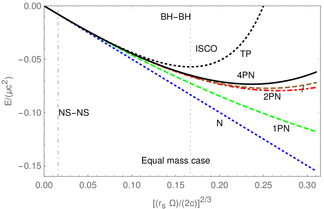
Figure 1: The energy of the last stable orbit in the quasi-circular case for equal masses. Dotted line: Newtonian case (N); Dashed line: 1PN; Dash-dotted line: 2PN; Upper dashed line: 3PN; Full line: 4PN; Upper dotted line: test particle solution (TP). Dashed vertical lines: range for the innermost stable circular orbit (ISCO), [58]. The other vertical lines mark the frequency spectrum for neutron star (NS) and black hole (BH) merging at LIGO.

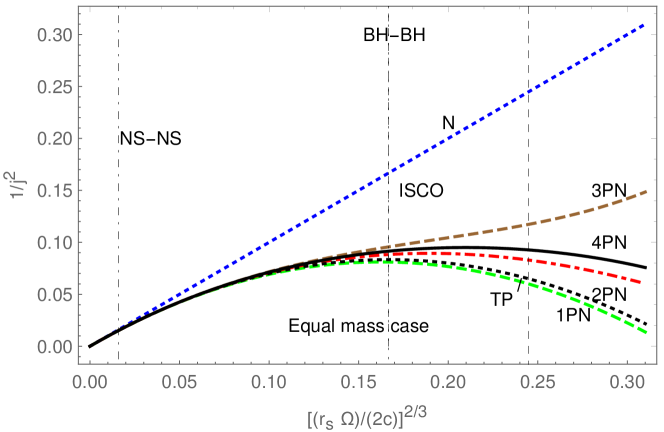
Figure 2: The angular momentum $1/j^{2}$; the labels correspond to Figure 1.

The test particle solution reads [18]

$$\frac{1}{j^{2}(x)} = x(1-3x).$$ (72)

Both relations (69,71) are well–known from the results of other calculations, cf. e.g. [18]. The position of the innermost stable circular orbit varies with $\nu$ [58]. In the limit $\nu\rightarrow 0$ it assumes $x=1/6$ and in the equal mass case at 4PN it reaches $x\approx 0.245$.

We have obtained agreement with the above relations by explicit calculation, which are illustrated in Figures 1–2. Here $r_{s}=2G_{N}M/c^{2}$ denotes the Schwarzschild radius. It is evident that even in the region of ISCO at 4PN convergence has not been reached and even higher order corrections are important. In these Figures we limited ourselves to the post–Newtonian approach. When extending the $x$-range, further matching to the results of other representations becomes necessary, cf. e.g. [59].

The final goal of the post–Newtonian calculations is the prediction of the oscillation signal due to gravitational waves in the detectors. This requires in addition to the Hamiltonian also the luminosity function $L$, cf. e.g. [60], which currently only allows to use the 3PN approximation on the Hamiltonian side, which we agree, cf. e.g. [60, 61].

6 Conclusions

We have calculated the Hamiltonian of two-body systems in an effective field theory approach to gravity to the fourth post–Newtonian order in harmonic coordinates using dimensional regularization. Here, starting with the third post–Newtonian order divergences in the dimensional regularization parameter $\varepsilon$ occur. However, these terms do not affect any observable. These are gauge- and coordinate system artifacts related to the regularization process. No renormalization of the observables related to the process under consideration is needed. We have also presented pole–free Hamiltonians, obtained after a canonical transformation. Already before similar calculations in harmonic coordinates were performed in Refs. [62, 12, 8]. The present calculation, however, cannot be compared literally to these, because of probable differences in Feynman rules and differences in total time derivatives, which are partly large contributions. We have checked for [8] that we obtain the same equation of motion for the $m$th order Lagrange density. Other differences lay in the elimination of the acceleration terms and their time derivatives by forming the first order effective Lagrangian. The approach in [12] (and references therein) in harmonic coordinates is not an effective field theory approach, but is based on the Fokker action [63]. However, we have shown by an explicit calculation, that the Lagrangian given [12] yield the same result for $E(\Omega)$ which we obtain.

We compared to other results obtained working in harmonic coordinates [12, 8], ADM coordinates [11] and EOB coordinates [13] and demonstrated equivalence on the Hamiltonian level by the construction of explicit canonical transformations. We have illustrated our results in the case of circular motion for $E(\Omega)$ and $j(\Omega)$. We also present the Hamiltonian resulting from harmonic coordinates up to $O(\varepsilon)$ after eliminating the acceleration by a shift in $D$ dimensions, which is useful for further higher order calculations.

Appendix A The 4PN Hamiltonian up to $O(\varepsilon)$

In the following we present the local Hamiltonian up to 4PN including the $O(\varepsilon)$ terms, a central result of the present calculation. In its details it also serves as an important input to higher order post–Newtonian calculations. We use the following abbreviations

$$\hat{r}=r\mu_{1},\leavevmode\nobreak\ \leavevmode\nobreak\ \leavevmode\nobreak\ \leavevmode\nobreak\ \leavevmode\nobreak\ S_{\varepsilon}=(4\pi)^{\varepsilon}\exp[\gamma_{E}\varepsilon],\leavevmode\nobreak\ \leavevmode\nobreak\ \leavevmode\nobreak\ \leavevmode\nobreak\ \leavevmode\nobreak\ \tilde{S}_{\varepsilon}=\pi^{\varepsilon}\exp[\gamma_{E}\varepsilon]$$ (73)

and obtain

$$H_{\text{N}}={} \frac{p_{1}^{2}}{2m_{1}}+\frac{p_{2}^{2}}{2m_{2}}+\tilde{S}_{\varepsilon}P_{10}\frac{G_{N}}{r}\,,$$ (74)

$$H_{\text{1PN}}={} -\frac{p_{1}^{4}}{8m_{1}^{3}}-\frac{p_{2}^{4}}{8m_{2}^{3}}+\tilde{S}_{\varepsilon}\bigg{\{}\bigg{[}\varepsilon\bigg{(}-\frac{3}{2}n.p_{1}n.p_{2}+\frac{p_{1}.p_{2}}{2}+n.p_{1}n.p_{2}\ln(2)+7p_{1}.p_{2}\ln(2)$$

$$+n.p_{1}n.p_{2}\ln(\hat{r})+7p_{1}.p_{2}\ln(\hat{r})+\frac{P_{168}m_{1}}{m_{2}}+\frac{P_{74}m_{2}}{m_{1}}\bigg{)}+\frac{1}{2}n.p_{1}n.p_{2}+\frac{7p_{1}.p_{2}}{2}$$

$$-\frac{3m_{2}p_{1}^{2}}{2m_{1}}-\frac{3m_{1}p_{2}^{2}}{2m_{2}}\bigg{]}\frac{G_{N}}{r}+P_{26}\left(\frac{G_{N}}{r}\right)^{2}S_{\varepsilon}\bigg{\}}\,,$$ (75)

$$H_{\text{2PN}}={} \frac{p_{1}^{6}}{16m_{1}^{5}}+\frac{p_{2}^{6}}{16m_{2}^{5}}+\tilde{S}_{\varepsilon}\bigg{\{}\bigg{[}\varepsilon\bigg{(}\frac{P_{86}}{m_{1}^{2}}+\frac{P_{253}m_{1}}{m_{2}^{3}}+\frac{P_{189}}{m_{2}^{2}}+\frac{P_{212}}{m_{1}m_{2}}+\frac{P_{107}m_{2}}{m_{1}^{3}}\bigg{)}+\frac{P_{63}}{m_{1}^{2}}+\frac{P_{153}}{m_{2}^{2}}$$

$$+\frac{P_{203}}{m_{1}m_{2}}+\frac{5m_{2}p_{1}^{4}}{8m_{1}^{3}}+\frac{5m_{1}p_{2}^{4}}{8m_{2}^{3}}\bigg{]}\frac{G_{N}}{r}+\bigg{[}\varepsilon\bigg{(}P_{162}m_{1}+\frac{P_{165}m_{1}^{2}}{m_{2}}+P_{68}m_{2}+\frac{P_{71}m_{2}^{2}}{m_{1}}\bigg{)}$$

$$+P_{132}m_{1}+\frac{P_{133}m_{1}^{2}}{m_{2}}+P_{48}m_{2}+\frac{P_{49}m_{2}^{2}}{m_{1}}\bigg{]}\left(\frac{G_{N}}{r}\right)^{2}S_{\varepsilon}+P_{27}\left(\frac{G_{N}}{r}\right)^{3}S_{\varepsilon}^{2}\bigg{\}}+\tilde{S}_{\varepsilon}^{2}\bigg{[}\varepsilon\bigg{(}$$

$$P_{173}m_{1}+\frac{P_{172}m_{1}^{2}}{m_{2}}+P_{78}m_{2}+\frac{P_{77}m_{2}^{2}}{m_{1}}\bigg{)}+P_{144}m_{1}+P_{57}m_{2}+\frac{9m_{2}^{2}p_{1}^{2}}{2m_{1}}+\frac{9m_{1}^{2}p_{2}^{2}}{2m_{2}}\bigg{]}\left(\frac{G_{N}}{r}\right)^{2}$$

$$+\tilde{S}_{\varepsilon}^{3}P_{12}\left(\frac{G_{N}}{r}\right)^{3}\,,$$ (76)

$$H_{\text{3PN}}={} -\frac{5p_{1}^{8}}{128m_{1}^{7}}-\frac{5p_{2}^{8}}{128m_{2}^{7}}+\tilde{S}_{\varepsilon}^{3}\bigg{\{}\bigg{[}\varepsilon\bigg{(}P_{156}m_{1}^{2}+\frac{P_{158}m_{1}^{3}}{m_{2}}+P_{157}m_{1}m_{2}+P_{65}m_{2}^{2}+\frac{P_{66}m_{2}^{3}}{m_{1}}\bigg{)}$$

$$+P_{127}m_{1}^{2}+P_{129}m_{1}m_{2}+P_{44}m_{2}^{2}-\frac{27m_{2}^{3}p_{1}^{2}}{2m_{1}}-\frac{27m_{1}^{3}p_{2}^{2}}{2m_{2}}\bigg{]}\left(\frac{G_{N}}{r}\right)^{3}+P_{37}\left(\frac{G_{N}}{r}\right)^{4}S_{\varepsilon}\bigg{\}}$$

$$+\tilde{S}_{\varepsilon}^{2}\bigg{\{}\bigg{[}\varepsilon\bigg{(}\frac{P_{214}}{m_{1}}+\frac{P_{252}m_{1}^{2}}{m_{2}^{3}}+\frac{P_{256}m_{1}}{m_{2}^{2}}+\frac{P_{215}}{m_{2}}+\frac{P_{109}m_{2}}{m_{1}^{2}}+\frac{P_{106}m_{2}^{2}}{m_{1}^{3}}\bigg{)}+\frac{P_{205}}{m_{1}}+\frac{P_{241}m_{1}}{m_{2}^{2}}$$

$$+\frac{P_{206}}{m_{2}}+\frac{P_{97}m_{2}}{m_{1}^{2}}-\frac{3m_{2}^{2}p_{1}^{4}}{4m_{1}^{3}}-\frac{3m_{1}^{2}p_{2}^{4}}{4m_{2}^{3}}\bigg{]}\left(\frac{G_{N}}{r}\right)^{2}+\bigg{[}\varepsilon\bigg{(}P_{184}m_{1}^{2}+\frac{P_{181}m_{1}^{3}}{m_{2}}+P_{182}m_{1}m_{2}$$

$$+P_{83}m_{2}^{2}+\frac{P_{81}m_{2}^{3}}{m_{1}}\bigg{)}+P_{148}m_{1}^{2}+\frac{P_{145}m_{1}^{3}}{m_{2}}+P_{147}m_{1}m_{2}+P_{60}m_{2}^{2}+\frac{P_{58}m_{2}^{3}}{m_{1}}\bigg{]}\left(\frac{G_{N}}{r}\right)^{3}S_{\varepsilon}$$

$$+P_{39}\left(\frac{G_{N}}{r}\right)^{4}S_{\varepsilon}^{2}\bigg{\}}+\tilde{S}_{\varepsilon}\bigg{\{}\bigg{[}\varepsilon\bigg{(}\frac{P_{113}}{m_{1}^{4}}+\frac{P_{283}m_{1}}{m_{2}^{5}}+\frac{P_{260}}{m_{2}^{4}}+\frac{P_{273}}{m_{1}m_{2}^{3}}+\frac{P_{217}}{m_{1}^{2}m_{2}^{2}}+\frac{P_{228}}{m_{1}^{3}m_{2}}$$

$$+\frac{P_{120}m_{2}}{m_{1}^{5}}\bigg{)}+\frac{P_{100}}{m_{1}^{4}}+\frac{P_{244}}{m_{2}^{4}}+\frac{P_{267}}{m_{1}m_{2}^{3}}+\frac{P_{208}}{m_{1}^{2}m_{2}^{2}}+\frac{P_{222}}{m_{1}^{3}m_{2}}-\frac{7m_{2}p_{1}^{6}}{16m_{1}^{5}}-\frac{7m_{1}p_{2}^{6}}{16m_{2}^{5}}\bigg{]}\frac{G_{N}}{r}$$

$$+\bigg{[}\varepsilon\bigg{(}\frac{P_{210}}{m_{1}}+\frac{P_{250}m_{1}^{2}}{m_{2}^{3}}+\frac{P_{251}m_{1}}{m_{2}^{2}}+\frac{P_{211}}{m_{2}}+\frac{P_{105}m_{2}}{m_{1}^{2}}+\frac{P_{104}m_{2}^{2}}{m_{1}^{3}}\bigg{)}+\frac{P_{201}}{m_{1}}+\frac{P_{237}m_{1}^{2}}{m_{2}^{3}}$$

$$+\frac{P_{238}m_{1}}{m_{2}^{2}}+\frac{P_{202}}{m_{2}}+\frac{P_{95}m_{2}}{m_{1}^{2}}+\frac{P_{94}m_{2}^{2}}{m_{1}^{3}}\bigg{]}\left(\frac{G_{N}}{r}\right)^{2}S_{\varepsilon}+\bigg{[}\pi^{2}P_{292}+\varepsilon\bigg{(}\pi^{2}P_{295}+P_{193}m_{1}^{2}$$

$$+\frac{P_{163}m_{1}^{3}}{m_{2}}+P_{192}m_{1}m_{2}+P_{88}m_{2}^{2}+\frac{P_{69}m_{2}^{3}}{m_{1}}\bigg{)}+P_{166}m_{1}^{2}+\frac{P_{135}m_{1}^{3}}{m_{2}}+P_{161}m_{1}m_{2}$$

$$+P_{72}m_{2}^{2}+\frac{P_{50}m_{2}^{3}}{m_{1}}\bigg{]}\left(\frac{G_{N}}{r}\right)^{3}S_{\varepsilon}^{2}+P_{38}\left(\frac{G_{N}}{r}\right)^{4}S_{\varepsilon}^{3}\bigg{\}}+\tilde{S}_{\varepsilon}^{4}P_{30}\left(\frac{G_{N}}{r}\right)^{4}\,,$$ (77)

$$H_{\text{4PN}}={} \frac{7p_{1}^{10}}{256m_{1}^{9}}+\frac{7p_{2}^{10}}{256m_{2}^{9}}+\tilde{S}_{\varepsilon}^{4}\bigg{\{}\bigg{[}\varepsilon\bigg{(}P_{187}m_{1}^{3}+\frac{P_{185}m_{1}^{4}}{m_{2}}+P_{188}m_{1}^{2}m_{2}+P_{186}m_{1}m_{2}^{2}+P_{85}m_{2}^{3}$$

$$+\frac{P_{84}m_{2}^{4}}{m_{1}}\bigg{)}+P_{150}m_{1}^{3}+P_{151}m_{1}^{2}m_{2}+P_{149}m_{1}m_{2}^{2}+P_{61}m_{2}^{3}+\frac{81m_{2}^{4}p_{1}^{2}}{2m_{1}}+\frac{81m_{1}^{4}p_{2}^{2}}{2m_{2}}\bigg{]}$$

$$\left(\frac{G_{N}}{r}\right)^{4}+P_{40}\left(\frac{G_{N}}{r}\right)^{5}S_{\varepsilon}\bigg{\}}+\tilde{S}_{\varepsilon}^{3}\bigg{\{}\bigg{[}\varepsilon\bigg{(}\frac{225}{4}(n.p_{1})^{3}n.p_{2}-\frac{92297}{30}(n.p_{1})^{2}(n.p_{2})^{2}$$

$$+\frac{225}{4}n.p_{1}(n.p_{2})^{3}+\frac{53}{2}(n.p_{1})^{2}p_{1}.p_{2}+\frac{2945849n.p_{1}n.p_{2}p_{1}.p_{2}}{1200}+\frac{53}{2}(n.p_{2})^{2}p_{1}.p_{2}$$

$$-\frac{496543(p_{1}.p_{2})^{2}}{1800}-\frac{177}{2}(n.p_{1})^{3}n.p_{2}\ln(2)+2473(n.p_{1})^{2}(n.p_{2})^{2}\ln(2)$$

$$-\frac{177}{2}n.p_{1}(n.p_{2})^{3}\ln(2)-\frac{1101}{4}(n.p_{1})^{2}p_{1}.p_{2}\ln(2)-\frac{103357}{40}n.p_{1}n.p_{2}p_{1}.p_{2}\ln(2)$$

$$-\frac{1101}{4}(n.p_{2})^{2}p_{1}.p_{2}\ln(2)-\frac{75359}{40}(p_{1}.p_{2})^{2}\ln(2)-\frac{177}{2}(n.p_{1})^{3}n.p_{2}\ln(\hat{r})$$

$$+2473(n.p_{1})^{2}(n.p_{2})^{2}\ln(\hat{r})-\frac{177}{2}n.p_{1}(n.p_{2})^{3}\ln(\hat{r})-\frac{1101}{4}(n.p_{1})^{2}p_{1}.p_{2}\ln(\hat{r})$$

$$-\frac{103357}{40}n.p_{1}n.p_{2}p_{1}.p_{2}\ln(\hat{r})-\frac{1101}{4}(n.p_{2})^{2}p_{1}.p_{2}\ln(\hat{r})-\frac{75359}{40}(p_{1}.p_{2})^{2}\ln(\hat{r})$$

$$+\frac{P_{247}m_{1}^{3}}{m_{2}^{3}}+\frac{P_{246}m_{1}^{2}}{m_{2}^{2}}+\frac{P_{245}m_{1}}{m_{2}}+\frac{P_{209}m_{2}}{m_{1}}+\frac{P_{101}m_{2}^{2}}{m_{1}^{2}}+\frac{P_{102}m_{2}^{3}}{m_{1}^{3}}-\frac{17525}{144}n.p_{1}n.p_{2}p_{1}^{2}$$

$$+\frac{1282037(n.p_{2})^{2}p_{1}^{2}}{2400}+\frac{25133}{432}p_{1}.p_{2}p_{1}^{2}+\frac{289}{2}n.p_{1}n.p_{2}\ln(2)p_{1}^{2}-\frac{24221}{80}(n.p_{2})^{2}\ln(2)p_{1}^{2}$$

$$+\frac{3490}{3}p_{1}.p_{2}\ln(2)p_{1}^{2}+\frac{289}{2}n.p_{1}n.p_{2}\ln(\hat{r})p_{1}^{2}-\frac{24221}{80}(n.p_{2})^{2}\ln(\hat{r})p_{1}^{2}$$

$$+\frac{3490}{3}p_{1}.p_{2}\ln(\hat{r})p_{1}^{2}+\frac{1282037(n.p_{1})^{2}p_{2}^{2}}{2400}-\frac{17525}{144}n.p_{1}n.p_{2}p_{2}^{2}+\frac{25133}{432}p_{1}.p_{2}p_{2}^{2}$$

$$-\frac{24221}{80}(n.p_{1})^{2}\ln(2)p_{2}^{2}+\frac{289}{2}n.p_{1}n.p_{2}\ln(2)p_{2}^{2}+\frac{3490}{3}p_{1}.p_{2}\ln(2)p_{2}^{2}$$

$$-\frac{24221}{80}(n.p_{1})^{2}\ln(\hat{r})p_{2}^{2}+\frac{289}{2}n.p_{1}n.p_{2}\ln(\hat{r})p_{2}^{2}+\frac{3490}{3}p_{1}.p_{2}\ln(\hat{r})p_{2}^{2}-\frac{145817}{900}p_{1}^{2}p_{2}^{2}$$

$$-\frac{49597}{40}\ln(2)p_{1}^{2}p_{2}^{2}-\frac{49597}{40}\ln(\hat{r})p_{1}^{2}p_{2}^{2}\bigg{)}-\frac{59}{4}(n.p_{1})^{3}n.p_{2}+\frac{2473}{6}(n.p_{1})^{2}(n.p_{2})^{2}$$

$$-\frac{59}{4}n.p_{1}(n.p_{2})^{3}-\frac{367}{8}(n.p_{1})^{2}p_{1}.p_{2}-\frac{103357}{240}n.p_{1}n.p_{2}p_{1}.p_{2}-\frac{367}{8}(n.p_{2})^{2}p_{1}.p_{2}$$

$$-\frac{75359}{240}(p_{1}.p_{2})^{2}+\frac{P_{234}m_{1}^{2}}{m_{2}^{2}}+\frac{P_{233}m_{1}}{m_{2}}+\frac{P_{200}m_{2}}{m_{1}}+\frac{P_{91}m_{2}^{2}}{m_{1}^{2}}+\frac{289}{12}n.p_{1}n.p_{2}p_{1}^{2}$$

$$-\frac{24221}{480}(n.p_{2})^{2}p_{1}^{2}+\frac{1745}{9}p_{1}.p_{2}p_{1}^{2}-\frac{45m_{2}^{3}p_{1}^{4}}{4m_{1}^{3}}-\frac{24221}{480}(n.p_{1})^{2}p_{2}^{2}+\frac{289}{12}n.p_{1}n.p_{2}p_{2}^{2}$$

$$+\frac{1745}{9}p_{1}.p_{2}p_{2}^{2}-\frac{49597}{240}p_{1}^{2}p_{2}^{2}-\frac{45m_{1}^{3}p_{2}^{4}}{4m_{2}^{3}}\bigg{]}\left(\frac{G_{N}}{r}\right)^{3}+\bigg{[}\varepsilon\bigg{(}\pi^{2}P_{291}+P_{190}m_{1}^{3}+\frac{P_{155}m_{1}^{4}}{m_{2}}$$

$$+P_{191}m_{1}^{2}m_{2}+P_{154}m_{1}m_{2}^{2}+P_{87}m_{2}^{3}+\frac{P_{64}m_{2}^{4}}{m_{1}}\bigg{)}+P_{159}m_{1}^{3}+\frac{P_{128}m_{1}^{4}}{m_{2}}+P_{160}m_{1}^{2}m_{2}$$

$$+P_{126}m_{1}m_{2}^{2}+P_{67}m_{2}^{3}+\frac{P_{45}m_{2}^{4}}{m_{1}}\bigg{]}\left(\frac{G_{N}}{r}\right)^{4}S_{\varepsilon}+P_{43}\left(\frac{G_{N}}{r}\right)^{5}S_{\varepsilon}^{2}\bigg{\}}+\tilde{S}_{\varepsilon}^{2}\bigg{\{}\bigg{[}$$

$$\varepsilon\bigg{(}\frac{P_{226}}{m_{1}^{3}}+\frac{P_{285}m_{1}^{2}}{m_{2}^{5}}+\frac{P_{286}m_{1}}{m_{2}^{4}}+\frac{P_{271}}{m_{2}^{3}}+\frac{P_{274}}{m_{1}m_{2}^{2}}+\frac{P_{229}}{m_{1}^{2}m_{2}}+\frac{P_{123}m_{2}}{m_{1}^{4}}+\frac{P_{122}m_{2}^{2}}{m_{1}^{5}}\bigg{)}+\frac{P_{220}}{m_{1}^{3}}$$

$$+\frac{P_{280}m_{1}}{m_{2}^{4}}+\frac{P_{265}}{m_{2}^{3}}+\frac{P_{268}}{m_{1}m_{2}^{2}}+\frac{P_{223}}{m_{1}^{2}m_{2}}+\frac{P_{117}m_{2}}{m_{1}^{4}}+\frac{23m_{2}^{2}p_{1}^{6}}{16m_{1}^{5}}+\frac{23m_{1}^{2}p_{2}^{6}}{16m_{2}^{5}}\bigg{]}\left(\frac{G_{N}}{r}\right)^{2}+\bigg{[}\varepsilon\bigg{(}$$

$$\pi^{2}\bigg{(}\frac{P_{236}m_{1}}{m_{2}}+\frac{P_{93}m_{2}}{m_{1}}-\frac{33}{8}n.p_{1}n.p_{2}p_{1}^{2}+\frac{11}{8}p_{1}.p_{2}p_{1}^{2}-\frac{33}{8}n.p_{1}n.p_{2}p_{2}^{2}+\frac{11}{8}p_{1}.p_{2}p_{2}^{2}\bigg{)}$$

$$-\frac{7219}{18}(n.p_{1})^{3}n.p_{2}+\frac{391051}{90}(n.p_{1})^{2}(n.p_{2})^{2}-\frac{7219}{18}n.p_{1}(n.p_{2})^{3}+\frac{568}{3}(n.p_{1})^{2}p_{1}.p_{2}$$

$$-\frac{188107}{90}n.p_{1}n.p_{2}p_{1}.p_{2}+\frac{568}{3}(n.p_{2})^{2}p_{1}.p_{2}+\frac{22691}{150}(p_{1}.p_{2})^{2}+278(n.p_{1})^{3}n.p_{2}\ln(2)$$

$$-\frac{8144}{3}(n.p_{1})^{2}(n.p_{2})^{2}\ln(2)+278n.p_{1}(n.p_{2})^{3}\ln(2)-24(n.p_{1})^{2}p_{1}.p_{2}\ln(2)$$

$$+\frac{3830}{3}n.p_{1}n.p_{2}p_{1}.p_{2}\ln(2)-24(n.p_{2})^{2}p_{1}.p_{2}\ln(2)+\frac{6518}{5}(p_{1}.p_{2})^{2}\ln(2)$$

$$+417(n.p_{1})^{3}n.p_{2}\ln(\hat{r})-4072(n.p_{1})^{2}(n.p_{2})^{2}\ln(\hat{r})+417n.p_{1}(n.p_{2})^{3}\ln(\hat{r})$$

$$-36(n.p_{1})^{2}p_{1}.p_{2}\ln(\hat{r})+1915n.p_{1}n.p_{2}p_{1}.p_{2}\ln(\hat{r})-36(n.p_{2})^{2}p_{1}.p_{2}\ln(\hat{r})$$

$$+\frac{9777}{5}(p_{1}.p_{2})^{2}\ln(\hat{r})+\frac{P_{258}m_{1}^{3}}{m_{2}^{3}}+\frac{P_{259}m_{1}^{2}}{m_{2}^{2}}+\frac{P_{261}m_{1}}{m_{2}}+\frac{P_{216}m_{2}}{m_{1}}+\frac{P_{112}m_{2}^{2}}{m_{1}^{2}}+\frac{P_{111}m_{2}^{3}}{m_{1}^{3}}$$

$$-\frac{9787}{144}n.p_{1}n.p_{2}p_{1}^{2}-\frac{113167}{360}(n.p_{2})^{2}p_{1}^{2}-\frac{17963}{432}p_{1}.p_{2}p_{1}^{2}+\frac{1475}{12}n.p_{1}n.p_{2}\ln(2)p_{1}^{2}$$

$$-\frac{29}{6}(n.p_{2})^{2}\ln(2)p_{1}^{2}-\frac{26015}{36}p_{1}.p_{2}\ln(2)p_{1}^{2}-44n.p_{1}n.p_{2}\ln^{2}(2)p_{1}^{2}+\frac{44}{3}p_{1}.p_{2}\ln^{2}(2)p_{1}^{2}$$

$$+\frac{1475}{8}n.p_{1}n.p_{2}\ln(\hat{r})p_{1}^{2}-\frac{29}{4}(n.p_{2})^{2}\ln(\hat{r})p_{1}^{2}-\frac{26015}{24}p_{1}.p_{2}\ln(\hat{r})p_{1}^{2}$$

$$-132n.p_{1}n.p_{2}\ln(2)\ln(\hat{r})p_{1}^{2}+44p_{1}.p_{2}\ln(2)\ln(\hat{r})p_{1}^{2}-99n.p_{1}n.p_{2}\ln^{2}(\hat{r})p_{1}^{2}$$

$$+33p_{1}.p_{2}\ln^{2}(\hat{r})p_{1}^{2}-\frac{113167}{360}(n.p_{1})^{2}p_{2}^{2}-\frac{9787}{144}n.p_{1}n.p_{2}p_{2}^{2}-\frac{17963}{432}p_{1}.p_{2}p_{2}^{2}$$

$$-\frac{29}{6}(n.p_{1})^{2}\ln(2)p_{2}^{2}+\frac{1475}{12}n.p_{1}n.p_{2}\ln(2)p_{2}^{2}-\frac{26015}{36}p_{1}.p_{2}\ln(2)p_{2}^{2}$$

$$-44n.p_{1}n.p_{2}\ln^{2}(2)p_{2}^{2}+\frac{44}{3}p_{1}.p_{2}\ln^{2}(2)p_{2}^{2}-\frac{29}{4}(n.p_{1})^{2}\ln(\hat{r})p_{2}^{2}$$

$$+\frac{1475}{8}n.p_{1}n.p_{2}\ln(\hat{r})p_{2}^{2}-\frac{26015}{24}p_{1}.p_{2}\ln(\hat{r})p_{2}^{2}-132n.p_{1}n.p_{2}\ln(2)\ln(\hat{r})p_{2}^{2}$$

$$+44p_{1}.p_{2}\ln(2)\ln(\hat{r})p_{2}^{2}-99n.p_{1}n.p_{2}\ln^{2}(\hat{r})p_{2}^{2}+33p_{1}.p_{2}\ln^{2}(\hat{r})p_{2}^{2}+\frac{7237}{225}p_{1}^{2}p_{2}^{2}$$

$$+\frac{13232}{15}\ln(2)p_{1}^{2}p_{2}^{2}+\frac{6616}{5}\ln(\hat{r})p_{1}^{2}p_{2}^{2}\bigg{)}+\frac{139}{2}(n.p_{1})^{3}n.p_{2}-\frac{2036}{3}(n.p_{1})^{2}(n.p_{2})^{2}$$

$$+\frac{139}{2}n.p_{1}(n.p_{2})^{3}-6(n.p_{1})^{2}p_{1}.p_{2}+\frac{1915}{6}n.p_{1}n.p_{2}p_{1}.p_{2}-6(n.p_{2})^{2}p_{1}.p_{2}+\frac{3259}{10}(p_{1}.p_{2})^{2}$$

$$+\frac{P_{242}m_{1}^{3}}{m_{2}^{3}}+\frac{P_{243}m_{1}^{2}}{m_{2}^{2}}+\frac{P_{249}m_{1}}{m_{2}}+\frac{P_{207}m_{2}}{m_{1}}+\frac{P_{99}m_{2}^{2}}{m_{1}^{2}}+\frac{P_{98}m_{2}^{3}}{m_{1}^{3}}+\frac{1475}{48}n.p_{1}n.p_{2}p_{1}^{2}$$

$$-\frac{29}{24}(n.p_{2})^{2}p_{1}^{2}-\frac{26015}{144}p_{1}.p_{2}p_{1}^{2}-22n.p_{1}n.p_{2}\ln(2)p_{1}^{2}+\frac{22}{3}p_{1}.p_{2}\ln(2)p_{1}^{2}$$

$$-33n.p_{1}n.p_{2}\ln(\hat{r})p_{1}^{2}+11p_{1}.p_{2}\ln(\hat{r})p_{1}^{2}-\frac{29}{24}(n.p_{1})^{2}p_{2}^{2}+\frac{1475}{48}n.p_{1}n.p_{2}p_{2}^{2}$$

$$-\frac{26015}{144}p_{1}.p_{2}p_{2}^{2}-22n.p_{1}n.p_{2}\ln(2)p_{2}^{2}+\frac{22}{3}p_{1}.p_{2}\ln(2)p_{2}^{2}-33n.p_{1}n.p_{2}\ln(\hat{r})p_{2}^{2}$$

$$+11p_{1}.p_{2}\ln(\hat{r})p_{2}^{2}+\frac{3308}{15}p_{1}^{2}p_{2}^{2}\bigg{]}\left(\frac{G_{N}}{r}\right)^{3}S_{\varepsilon}+\bigg{[}\pi^{2}P_{294}+\varepsilon\bigg{(}\pi^{2}P_{297}+P_{199}m_{1}^{3}+\frac{P_{183}m_{1}^{4}}{m_{2}}$$

$$+P_{198}m_{1}^{2}m_{2}+P_{197}m_{1}m_{2}^{2}+P_{90}m_{2}^{3}+\frac{P_{82}m_{2}^{4}}{m_{1}}\bigg{)}+P_{179}m_{1}^{3}+\frac{P_{146}m_{1}^{4}}{m_{2}}+P_{178}m_{1}^{2}m_{2}$$

$$+P_{177}m_{1}m_{2}^{2}+P_{80}m_{2}^{3}+\frac{P_{59}m_{2}^{4}}{m_{1}}\bigg{]}\left(\frac{G_{N}}{r}\right)^{4}S_{\varepsilon}^{2}+P_{42}\left(\frac{G_{N}}{r}\right)^{5}S_{\varepsilon}^{3}\bigg{\}}+\tilde{S}_{\varepsilon}\bigg{\{}\bigg{[}$$

$$\varepsilon\bigg{(}\frac{P_{124}}{m_{1}^{6}}+\frac{P_{290}m_{1}}{m_{2}^{7}}+\frac{P_{287}}{m_{2}^{6}}+\frac{P_{289}}{m_{1}m_{2}^{5}}+\frac{P_{275}}{m_{1}^{2}m_{2}^{4}}+\frac{P_{277}}{m_{1}^{3}m_{2}^{3}}+\frac{P_{230}}{m_{1}^{4}m_{2}^{2}}+\frac{P_{232}}{m_{1}^{5}m_{2}}+\frac{P_{125}m_{2}}{m_{1}^{7}}\bigg{)}$$

$$+\frac{P_{118}}{m_{1}^{6}}+\frac{P_{281}}{m_{2}^{6}}+\frac{P_{288}}{m_{1}m_{2}^{5}}+\frac{P_{269}}{m_{1}^{2}m_{2}^{4}}+\frac{P_{276}}{m_{1}^{3}m_{2}^{3}}+\frac{P_{224}}{m_{1}^{4}m_{2}^{2}}+\frac{P_{231}}{m_{1}^{5}m_{2}}+\frac{45m_{2}p_{1}^{8}}{128m_{1}^{7}}+\frac{45m_{1}p_{2}^{8}}{128m_{2}^{7}}\bigg{]}\frac{G_{N}}{r}$$

$$+\bigg{[}\varepsilon\bigg{(}\frac{P_{227}}{m_{1}^{3}}+\frac{P_{284}m_{1}^{2}}{m_{2}^{5}}+\frac{P_{282}m_{1}}{m_{2}^{4}}+\frac{P_{272}}{m_{2}^{3}}+\frac{P_{270}}{m_{1}m_{2}^{2}}+\frac{P_{225}}{m_{1}^{2}m_{2}}+\frac{P_{119}m_{2}}{m_{1}^{4}}+\frac{P_{121}m_{2}^{2}}{m_{1}^{5}}\bigg{)}$$

$$+\frac{P_{221}}{m_{1}^{3}}+\frac{P_{279}m_{1}^{2}}{m_{2}^{5}}+\frac{P_{278}m_{1}}{m_{2}^{4}}+\frac{P_{266}}{m_{2}^{3}}+\frac{P_{264}}{m_{1}m_{2}^{2}}+\frac{P_{219}}{m_{1}^{2}m_{2}}+\frac{P_{115}m_{2}}{m_{1}^{4}}+\frac{P_{116}m_{2}^{2}}{m_{1}^{5}}\bigg{]}\left(\frac{G_{N}}{r}\right)^{2}S_{\varepsilon}$$

$$+\bigg{[}\pi^{2}\bigg{(}\frac{15945}{512}(n.p_{1})^{2}(n.p_{2})^{2}-\frac{1635}{128}n.p_{1}n.p_{2}p_{1}.p_{2}+\frac{27}{256}(p_{1}.p_{2})^{2}+\frac{P_{239}m_{1}^{2}}{m_{2}^{2}}+\frac{P_{152}m_{1}}{m_{2}}$$

$$+\frac{P_{62}m_{2}}{m_{1}}+\frac{P_{96}m_{2}^{2}}{m_{1}^{2}}-\frac{1215}{512}(n.p_{2})^{2}p_{1}^{2}-\frac{1215}{512}(n.p_{1})^{2}p_{2}^{2}-\frac{253}{512}p_{1}^{2}p_{2}^{2}\bigg{)}+\varepsilon\bigg{(}\pi^{2}\bigg{(}$$

$$-35(n.p_{1})^{3}n.p_{2}-\frac{174061}{512}(n.p_{1})^{2}(n.p_{2})^{2}-35n.p_{1}(n.p_{2})^{3}+\frac{97}{5}(n.p_{1})^{2}p_{1}.p_{2}$$

$$+\frac{19315}{128}n.p_{1}n.p_{2}p_{1}.p_{2}+\frac{97}{5}(n.p_{2})^{2}p_{1}.p_{2}-\frac{21471(p_{1}.p_{2})^{2}}{1280}+\frac{47835}{256}(n.p_{1})^{2}(n.p_{2})^{2}\ln(2)$$

$$-\frac{4905}{64}n.p_{1}n.p_{2}p_{1}.p_{2}\ln(2)+\frac{81}{128}(p_{1}.p_{2})^{2}\ln(2)+\frac{47835}{256}(n.p_{1})^{2}(n.p_{2})^{2}\ln(\hat{r})$$

$$-\frac{4905}{64}n.p_{1}n.p_{2}p_{1}.p_{2}\ln(\hat{r})+\frac{81}{128}(p_{1}.p_{2})^{2}\ln(\hat{r})+\frac{P_{254}m_{1}^{2}}{m_{2}^{2}}+\frac{P_{240}m_{1}}{m_{2}}+\frac{P_{204}m_{2}}{m_{1}}$$

$$+\frac{P_{108}m_{2}^{2}}{m_{1}^{2}}+\frac{319}{20}n.p_{1}n.p_{2}p_{1}^{2}+\frac{43021(n.p_{2})^{2}p_{1}^{2}}{2560}-\frac{287}{60}p_{1}.p_{2}p_{1}^{2}-\frac{3645}{256}(n.p_{2})^{2}\ln(2)p_{1}^{2}$$

$$-\frac{3645}{256}(n.p_{2})^{2}\ln(\hat{r})p_{1}^{2}+\frac{43021(n.p_{1})^{2}p_{2}^{2}}{2560}+\frac{319}{20}n.p_{1}n.p_{2}p_{2}^{2}-\frac{287}{60}p_{1}.p_{2}p_{2}^{2}$$

$$-\frac{3645}{256}(n.p_{1})^{2}\ln(2)p_{2}^{2}-\frac{3645}{256}(n.p_{1})^{2}\ln(\hat{r})p_{2}^{2}+\frac{8827p_{1}^{2}p_{2}^{2}}{1536}-\frac{759}{256}\ln(2)p_{1}^{2}p_{2}^{2}$$

$$-\frac{759}{256}\ln(\hat{r})p_{1}^{2}p_{2}^{2}\bigg{)}-\frac{125231}{90}(n.p_{1})^{3}n.p_{2}+\frac{160115}{24}(n.p_{1})^{2}(n.p_{2})^{2}-\frac{125231}{90}n.p_{1}(n.p_{2})^{3}$$

$$+\frac{1818287(n.p_{1})^{2}p_{1}.p_{2}}{3375}-\frac{263129}{45}n.p_{1}n.p_{2}p_{1}.p_{2}+\frac{1818287(n.p_{2})^{2}p_{1}.p_{2}}{3375}$$

$$+\frac{12737819(p_{1}.p_{2})^{2}}{13500}+\frac{2215}{3}(n.p_{1})^{3}n.p_{2}\ln(2)-\frac{168443}{60}(n.p_{1})^{2}(n.p_{2})^{2}\ln(2)$$

$$+\frac{2215}{3}n.p_{1}(n.p_{2})^{3}\ln(2)-\frac{75172}{225}(n.p_{1})^{2}p_{1}.p_{2}\ln(2)+\frac{38974}{15}n.p_{1}n.p_{2}p_{1}.p_{2}\ln(2)$$

$$-\frac{75172}{225}(n.p_{2})^{2}p_{1}.p_{2}\ln(2)-\frac{282017}{450}(p_{1}.p_{2})^{2}\ln(2)-\frac{280}{3}(n.p_{1})^{3}n.p_{2}\ln^{2}(2)$$

$$+300(n.p_{1})^{2}(n.p_{2})^{2}\ln^{2}(2)-\frac{280}{3}n.p_{1}(n.p_{2})^{3}\ln^{2}(2)+\frac{776}{15}(n.p_{1})^{2}p_{1}.p_{2}\ln^{2}(2)$$

$$-176n.p_{1}n.p_{2}p_{1}.p_{2}\ln^{2}(2)+\frac{776}{15}(n.p_{2})^{2}p_{1}.p_{2}\ln^{2}(2)+\frac{56}{3}(p_{1}.p_{2})^{2}\ln^{2}(2)$$

$$+2215(n.p_{1})^{3}n.p_{2}\ln(\hat{r})-\frac{168443}{20}(n.p_{1})^{2}(n.p_{2})^{2}\ln(\hat{r})+2215n.p_{1}(n.p_{2})^{3}\ln(\hat{r})$$

$$-\frac{75172}{75}(n.p_{1})^{2}p_{1}.p_{2}\ln(\hat{r})+\frac{38974}{5}n.p_{1}n.p_{2}p_{1}.p_{2}\ln(\hat{r})-\frac{75172}{75}(n.p_{2})^{2}p_{1}.p_{2}\ln(\hat{r})$$

$$-\frac{282017}{150}(p_{1}.p_{2})^{2}\ln(\hat{r})-560(n.p_{1})^{3}n.p_{2}\ln(2)\ln(\hat{r})$$

$$+1800(n.p_{1})^{2}(n.p_{2})^{2}\ln(2)\ln(\hat{r})-560n.p_{1}(n.p_{2})^{3}\ln(2)\ln(\hat{r})$$

$$+\frac{1552}{5}(n.p_{1})^{2}p_{1}.p_{2}\ln(2)\ln(\hat{r})-1056n.p_{1}n.p_{2}p_{1}.p_{2}\ln(2)\ln(\hat{r})$$

$$+\frac{1552}{5}(n.p_{2})^{2}p_{1}.p_{2}\ln(2)\ln(\hat{r})+112(p_{1}.p_{2})^{2}\ln(2)\ln(\hat{r})-840(n.p_{1})^{3}n.p_{2}\ln^{2}(\hat{r})$$

$$+2700(n.p_{1})^{2}(n.p_{2})^{2}\ln^{2}(\hat{r})-840n.p_{1}(n.p_{2})^{3}\ln^{2}(\hat{r})+\frac{2328}{5}(n.p_{1})^{2}p_{1}.p_{2}\ln^{2}(\hat{r})$$

$$-1584n.p_{1}n.p_{2}p_{1}.p_{2}\ln^{2}(\hat{r})+\frac{2328}{5}(n.p_{2})^{2}p_{1}.p_{2}\ln^{2}(\hat{r})+168(p_{1}.p_{2})^{2}\ln^{2}(\hat{r})$$

$$+\frac{P_{248}m_{1}^{3}}{m_{2}^{3}}+\frac{P_{263}m_{1}^{2}}{m_{2}^{2}}+\frac{P_{262}m_{1}}{m_{2}}+\frac{P_{218}m_{2}}{m_{1}}+\frac{P_{114}m_{2}^{2}}{m_{1}^{2}}+\frac{P_{103}m_{2}^{3}}{m_{1}^{3}}+\frac{2713489n.p_{1}n.p_{2}p_{1}^{2}}{5400}$$

$$-\frac{13943393(n.p_{2})^{2}p_{1}^{2}}{9000}-\frac{605699p_{1}.p_{2}p_{1}^{2}}{9000}-\frac{284573}{900}n.p_{1}n.p_{2}\ln(2)p_{1}^{2}$$

$$+\frac{220249}{300}(n.p_{2})^{2}\ln(2)p_{1}^{2}+\frac{97787}{900}p_{1}.p_{2}\ln(2)p_{1}^{2}+\frac{638}{15}n.p_{1}n.p_{2}\ln^{2}(2)p_{1}^{2}$$

$$-92(n.p_{2})^{2}\ln^{2}(2)p_{1}^{2}-\frac{574}{45}p_{1}.p_{2}\ln^{2}(2)p_{1}^{2}-\frac{284573}{300}n.p_{1}n.p_{2}\ln(\hat{r})p_{1}^{2}$$

$$+\frac{220249}{100}(n.p_{2})^{2}\ln(\hat{r})p_{1}^{2}+\frac{97787}{300}p_{1}.p_{2}\ln(\hat{r})p_{1}^{2}+\frac{1276}{5}n.p_{1}n.p_{2}\ln(2)\ln(\hat{r})p_{1}^{2}$$

$$-552(n.p_{2})^{2}\ln(2)\ln(\hat{r})p_{1}^{2}-\frac{1148}{15}p_{1}.p_{2}\ln(2)\ln(\hat{r})p_{1}^{2}+\frac{1914}{5}n.p_{1}n.p_{2}\ln^{2}(\hat{r})p_{1}^{2}$$

$$-828(n.p_{2})^{2}\ln^{2}(\hat{r})p_{1}^{2}-\frac{574}{5}p_{1}.p_{2}\ln^{2}(\hat{r})p_{1}^{2}-\frac{13943393(n.p_{1})^{2}p_{2}^{2}}{9000}$$

$$+\frac{2713489n.p_{1}n.p_{2}p_{2}^{2}}{5400}-\frac{605699p_{1}.p_{2}p_{2}^{2}}{9000}+\frac{220249}{300}(n.p_{1})^{2}\ln(2)p_{2}^{2}$$

$$-\frac{284573}{900}n.p_{1}n.p_{2}\ln(2)p_{2}^{2}+\frac{97787}{900}p_{1}.p_{2}\ln(2)p_{2}^{2}-92(n.p_{1})^{2}\ln^{2}(2)p_{2}^{2}$$

$$+\frac{638}{15}n.p_{1}n.p_{2}\ln^{2}(2)p_{2}^{2}-\frac{574}{45}p_{1}.p_{2}\ln^{2}(2)p_{2}^{2}+\frac{220249}{100}(n.p_{1})^{2}\ln(\hat{r})p_{2}^{2}$$

$$-\frac{284573}{300}n.p_{1}n.p_{2}\ln(\hat{r})p_{2}^{2}+\frac{97787}{300}p_{1}.p_{2}\ln(\hat{r})p_{2}^{2}-552(n.p_{1})^{2}\ln(2)\ln(\hat{r})p_{2}^{2}$$

$$+\frac{1276}{5}n.p_{1}n.p_{2}\ln(2)\ln(\hat{r})p_{2}^{2}-\frac{1148}{15}p_{1}.p_{2}\ln(2)\ln(\hat{r})p_{2}^{2}-828(n.p_{1})^{2}\ln^{2}(\hat{r})p_{2}^{2}$$

$$+\frac{1914}{5}n.p_{1}n.p_{2}\ln^{2}(\hat{r})p_{2}^{2}-\frac{574}{5}p_{1}.p_{2}\ln^{2}(\hat{r})p_{2}^{2}+\frac{2824193p_{1}^{2}p_{2}^{2}}{5400}-\frac{3685}{12}\ln(2)p_{1}^{2}p_{2}^{2}$$

$$+\frac{124}{3}\ln^{2}(2)p_{1}^{2}p_{2}^{2}-\frac{3685}{4}\ln(\hat{r})p_{1}^{2}p_{2}^{2}+248\ln(2)\ln(\hat{r})p_{1}^{2}p_{2}^{2}+372\ln^{2}(\hat{r})p_{1}^{2}p_{2}^{2}\bigg{)}$$

$$+\frac{2215}{6}(n.p_{1})^{3}n.p_{2}-\frac{168443}{120}(n.p_{1})^{2}(n.p_{2})^{2}+\frac{2215}{6}n.p_{1}(n.p_{2})^{3}-\frac{37586}{225}(n.p_{1})^{2}p_{1}.p_{2}$$

$$+\frac{19487}{15}n.p_{1}n.p_{2}p_{1}.p_{2}-\frac{37586}{225}(n.p_{2})^{2}p_{1}.p_{2}-\frac{282017}{900}(p_{1}.p_{2})^{2}-\frac{280}{3}(n.p_{1})^{3}n.p_{2}\ln(2)$$

$$+300(n.p_{1})^{2}(n.p_{2})^{2}\ln(2)-\frac{280}{3}n.p_{1}(n.p_{2})^{3}\ln(2)+\frac{776}{15}(n.p_{1})^{2}p_{1}.p_{2}\ln(2)$$

$$-176n.p_{1}n.p_{2}p_{1}.p_{2}\ln(2)+\frac{776}{15}(n.p_{2})^{2}p_{1}.p_{2}\ln(2)+\frac{56}{3}(p_{1}.p_{2})^{2}\ln(2)$$

$$-280(n.p_{1})^{3}n.p_{2}\ln(\hat{r})+900(n.p_{1})^{2}(n.p_{2})^{2}\ln(\hat{r})-280n.p_{1}(n.p_{2})^{3}\ln(\hat{r})$$

$$+\frac{776}{5}(n.p_{1})^{2}p_{1}.p_{2}\ln(\hat{r})-528n.p_{1}n.p_{2}p_{1}.p_{2}\ln(\hat{r})+\frac{776}{5}(n.p_{2})^{2}p_{1}.p_{2}\ln(\hat{r})$$

$$+56(p_{1}.p_{2})^{2}\ln(\hat{r})+\frac{P_{235}m_{1}^{3}}{m_{2}^{3}}+\frac{P_{257}m_{1}^{2}}{m_{2}^{2}}+\frac{P_{255}m_{1}}{m_{2}}+\frac{P_{213}m_{2}}{m_{1}}+\frac{P_{110}m_{2}^{2}}{m_{1}^{2}}+\frac{P_{92}m_{2}^{3}}{m_{1}^{3}}$$

$$-\frac{284573n.p_{1}n.p_{2}p_{1}^{2}}{1800}+\frac{220249}{600}(n.p_{2})^{2}p_{1}^{2}+\frac{97787p_{1}.p_{2}p_{1}^{2}}{1800}+\frac{638}{15}n.p_{1}n.p_{2}\ln(2)p_{1}^{2}$$

$$-92(n.p_{2})^{2}\ln(2)p_{1}^{2}-\frac{574}{45}p_{1}.p_{2}\ln(2)p_{1}^{2}+\frac{638}{5}n.p_{1}n.p_{2}\ln(\hat{r})p_{1}^{2}-276(n.p_{2})^{2}\ln(\hat{r})p_{1}^{2}$$

$$-\frac{574}{15}p_{1}.p_{2}\ln(\hat{r})p_{1}^{2}+\frac{220249}{600}(n.p_{1})^{2}p_{2}^{2}-\frac{284573n.p_{1}n.p_{2}p_{2}^{2}}{1800}+\frac{97787p_{1}.p_{2}p_{2}^{2}}{1800}$$

$$-92(n.p_{1})^{2}\ln(2)p_{2}^{2}+\frac{638}{15}n.p_{1}n.p_{2}\ln(2)p_{2}^{2}-\frac{574}{45}p_{1}.p_{2}\ln(2)p_{2}^{2}-276(n.p_{1})^{2}\ln(\hat{r})p_{2}^{2}$$

$$+\frac{638}{5}n.p_{1}n.p_{2}\ln(\hat{r})p_{2}^{2}-\frac{574}{15}p_{1}.p_{2}\ln(\hat{r})p_{2}^{2}-\frac{3685}{24}p_{1}^{2}p_{2}^{2}+\frac{124}{3}\ln(2)p_{1}^{2}p_{2}^{2}$$

$$+124\ln(\hat{r})p_{1}^{2}p_{2}^{2}\bigg{]}\left(\frac{G_{N}}{r}\right)^{3}S_{\varepsilon}^{2}+\bigg{[}\pi^{2}P_{293}+\varepsilon\bigg{(}\pi^{2}P_{296}+P_{195}m_{1}^{3}+\frac{P_{164}m_{1}^{4}}{m_{2}}$$

$$+P_{194}m_{1}^{2}m_{2}+P_{196}m_{1}m_{2}^{2}+P_{89}m_{2}^{3}+\frac{P_{70}m_{2}^{4}}{m_{1}}\bigg{)}+P_{171}m_{1}^{3}+\frac{P_{136}m_{1}^{4}}{m_{2}}+P_{169}m_{1}^{2}m_{2}$$

$$+P_{175}m_{1}m_{2}^{2}+P_{76}m_{2}^{3}+\frac{P_{51}m_{2}^{4}}{m_{1}}\bigg{]}\left(\frac{G_{N}}{r}\right)^{4}S_{\varepsilon}^{3}+P_{41}\left(\frac{G_{N}}{r}\right)^{5}S_{\varepsilon}^{4}\bigg{\}}+\tilde{S}_{\varepsilon}^{5}P_{34}\left(\frac{G_{N}}{r}\right)^{5}.$$ (78)

Acknowledgment. We thank S. Foffa and R. Sturani for a discussion on Ref. [8] and Th. Damour, L. Blanchet, K. Schönwald and J. Steinhoff for different discussions. This work has been funded in part by EU TMR network SAGEX agreement No. 764850 (Marie Skłodowska-Curie) and COST action CA16201: Unraveling new physics at the LHC through the precision frontier. G. Schäfer has been supported in part by Kolleg Mathematik Physik Berlin (KMPB). Part of the text has been typesetted using SigmaToTeX of the package Sigma [64, 65].

References

• [1] B.P. Abbott et al. [LIGO Scientific and Virgo Collaborations], Phys. Rev. X 6 (2016) no.4, 041015 Erratum: [Phys. Rev. X 8 (2018) no.3, 039903] [arXiv:1606.04856 [gr-qc]]; Phys. Rev. X 9 (2019) no.3, 031040 [arXiv:1811.12907 [astro-ph.HE]].
• [2] B. Kol and M. Smolkin, Class. Quant. Grav.  25 (2008) 145011 [arXiv:0712.4116 [hep-th]];
M. Levi, Rep. Progr. Phys. in print [arXiv:1807.01699 [hep-th]].
• [3] W.D. Goldberger and I.Z. Rothstein, Phys. Rev. D 73 (2006) 104029 [hep-th/0409156].
• [4] J.B. Gilmore and A. Ross, Phys. Rev. D 78 (2008) 124021 [arXiv:0810.1328 [gr-qc]].
• [5] S. Foffa and R. Sturani, Phys. Rev. D 84 (2011) 044031 [arXiv:1104.1122 [gr-qc]].
• [6] S. Foffa, P. Mastrolia, R. Sturani, C. Sturm and W. J. Torres Bobadilla, Phys. Rev. Lett.  122 (2019) no.24, 241605 [arXiv:1902.10571 [gr-qc]].
• [7] J. Blümlein, A. Maier and P. Marquard, Phys. Lett. B 800 (2020) 135100 [arXiv:1902.11180 [gr-qc]].
• [8] S. Foffa and R. Sturani, Phys. Rev. D 100 (2019) no.2, 024047 [arXiv:1903.05113 [gr-qc]].
• [9] S. Foffa, R.A. Porto, I. Rothstein and R. Sturani, Phys. Rev. D 100 (2019) no.2, 024048 [arXiv:1903.05118 [gr-qc]].
• [10] S. Foffa and R. Sturani, Hereditary Terms at Next-To-Leading Order in Two-Body Gravitational Dynamics, arXiv:1907.02869 [gr-qc];
L. Blanchet, S. Foffa, F. Larrouturou and R. Sturani, Logarithmic tail contributions to the energy function of circular compact binaries, arXiv:1912.12359 [gr-qc].
• [11] T. Damour, P. Jaranowski and G. Schäfer, Phys. Rev. D 89 (2014) no.6, 064058 [arXiv:1401.4548 [gr-qc]].
• [12] L. Bernard, L. Blanchet, G. Faye and T. Marchand, Phys. Rev. D 97 (2018) no.4, 044037 [arXiv:1711.00283 [gr-qc]].
• [13] D. Bini, T. Damour and A. Geralico, Phys. Rev. Lett.  123 (2019) no.23, 231104 [arXiv:1909.02375 [gr-qc]] and references therein.
• [14] R. Clausius, Ann. Phys. (Leipzig) 217 (1870) 124–130;
H. Stephani and G. Kluge, Grundlagen der theoretischen Mechanik (DVW, Berlin, 1975).
• [15] Z. Bern, C. Cheung, R. Roiban, C.H. Shen, M.P. Solon and M. Zeng, JHEP 1910 (2019) 206 [arXiv:1908.01493 [hep-th]]; Phys. Rev. Lett.  122 (2019) no.20, 201603 [arXiv:1901.04424 [hep-th]].
• [16] T. Damour, Classical and Quantum Scattering in Post-Minkowskian Gravity, arXiv:1912.02139 [gr-qc].
• [17] C. Cheung, I.Z. Rothstein and M.P. Solon, Phys. Rev. Lett.  121 (2018) no.25, 251101 [arXiv:1808.02489 [hep-th]];
Phys. Rev. D 97 (2018) no.4, 044038 [arXiv:1710.10599 [gr-qc]];
T. Damour, Phys. Rev. D 94 (2016) no.10, 104015 [arXiv:1609.00354 [gr-qc]]; Phys. Rev. D 97 (2018) no.4, 044038 [arXiv:1710.10599 [gr-qc]];
N.E.J. Bjerrum-Bohr, P.H. Damgaard, G. Festuccia, L. Planté and P. Vanhove, Phys. Rev. Lett.  121 (2018) no.17, 171601 [arXiv:1806.04920 [hep-th]];
A. Koemans Collado, P. Di Vecchia and R. Russo, Phys. Rev. D 100 (2019) no.6, 066028 [arXiv:1904.02667 [hep-th]];
A. Cristofoli, N.E.J. Bjerrum-Bohr, P.H. Damgaard and P. Vanhove, Phys. Rev. D 100 (2019) no.8, 084040 [arXiv:1906.01579 [hep-th]];
N.E.J. Bjerrum-Bohr, A. Cristofoli and P.H. Damgaard, arXiv:1910.09366 [hep-th];
J. Blümlein, A. Maier, P. Marquard, G. Schäfer and C. Schneider, Phys. Lett. B 801 (2020) 135157 [arXiv:1911.04411 [gr-qc]].
• [18] G. Schäfer and P. Jaranowski, Living Rev. Rel.  21 (2018) no.1, 7, 1–117 [arXiv:1805.07240 [gr-qc]].
• [19] P. Nogueira, J. Comput. Phys.  105 (1993) 279–289.
• [20] J.A.M. Vermaseren, New features of FORM, math-ph/0010025;
M. Tentyukov and J.A.M. Vermaseren, Comput. Phys. Commun.  181 (2010) 1419–1427 [hep-ph/0702279].
• [21] P. Marquard and D. Seidel, The Crusher algorithm, unpublished.
• [22] S. Foffa and R. Sturani, Phys. Rev. D 87 (2013) no.6, 064011 [arXiv:1206.7087 [gr-qc]].
• [23] E. Schmutzer, Grundprinzipien der klassischen Mechanik und der klassischen Feldtheorie, (DVW, Berlin, 1973).
• [24] R.A. Porto and I.Z. Rothstein, Phys. Rev. D 96 (2017) no.2, 024062 [arXiv:1703.06433 [gr-qc]].
• [25] T. Damour and G. Schäfer, Gen. Rel. Grav.  17 (1985) 879–905.
• [26] B.S. DeWitt, Dynamical Theory of Groups and Fields in Relativiy, Groups and Topology, Eds. C. DeWitt and B. DeWitt, (Gordon and Breach, New York, 1964), Eq. (18.1).
• [27] T. Damour and G. Schäfer, J. Math. Phys.  32 (1991) 127–134.
• [28] T. Marchand, L. Bernard, L. Blanchet and G. Faye, Phys. Rev. D 97 (2018) no.4, 044023 [arXiv:1707.09289 [gr-qc]].
• [29] G. Schäfer, Astron. Nachr. 311 (1990) 213–217.
• [30] T. Damour, P. Jaranowski and G. Schäfer, Phys. Rev. D 93 (2016) no.8, 084014 [arXiv:1601.01283 [gr-qc]].
• [31] L. Blanchet and T. Damour, Phys. Rev. D 37 (1988) 1410–1435.
• [32] S. Foffa and R. Sturani, Phys. Rev. D 87 (2013) no.4, 044056 [arXiv:1111.5488 [gr-qc]].
• [33] C. R. Galley, A. K. Leibovich, R. A. Porto and A. Ross, Phys. Rev. D 93 (2016) 124010 [arXiv:1511.07379 [gr-qc]].
• [34] L. Bernard, L. Blanchet, A. Bohé, G. Faye and S. Marsat, Phys. Rev. D 96 (2017) no.10, 104043 [arXiv:1706.08480 [gr-qc]].
• [35] P. Jaranowski and G. Schäfer, Phys. Rev. D 92 (2015) no.12, 124043 [arXiv:1508.01016 [gr-qc]].
• [36] J. Lützen, The Prehistory of the Theory of Distributions, (Springer, New York, 1982).
• [37] J. Hadamard, Le problème de Cauchy et les équations aux dérivées partielles linéaires hyperboliques, (Hermann et Cie., Paris, 1932);
J. Naas, H.L. Schmid, Mathematisches Wörterbuch, (Akademie Verlag, Berlin, 1961), Vol. I, p. 448.
• [38] V.S. Vladimirov, Gleichungen der mathematischen Physik, (DVW, Berlin, 1972).
• [39] S. Weinberg, Gravitation and Cosmology, Principles and Applications of the General Theory of Relativity, (J. Wiley & Sons, Hoboken, NJ, 1972).
• [40] E. Schmutzer, Relativistische Physik, (Teubner, Leipzig, 1968).
• [41] K. Symanzik, Commun. Math. Phys.  18 (1970) 227–246.
• [42] C.G. Callan, Jr., Phys. Rev. D 2 (1970) 1541–1547.
• [43] J. Alvey, N. Sabti, M. Escudero and M. Fairbairn, Improved BBN Constraints on the Variation of the Gravitational Constant, arXiv:1910.10730 [astro-ph.CO].
• [44] P. Mittelstädt, Klassische Mechanik, 2nd Ed., BI Vol. 500, (BI Wissenschaftsverlag, Mannheim, 1995). k
• [45] W. Gröbner, Die Lie-Reihen und ihre Anwendungen, (DVW, Berlin, 1960).
• [46] J.P. Vinti, Orbital and Celestial Mechanics. Progress in Astronautics and Aeronautics, 177, (1998) American Institute of Aeronautics and Astronautics, Reston, VA, G.J Der and N.L Bonavito (Eds.).
• [47] C.G. Jacobi, Vorlesungen über analytische Mechanik, nach einer Mitschrift von Wilhelm Scheibner, Friedrich Wilhelms Universität Berlin 1847/48, Ed. H.  Pulte, (Vieweg, Wiesbaden, 1996).
• [48] W. Killing, Math. Ann. 31 (1888) 252–290; 33 (1889) 1–48; 34 (1889) 57–122; 36 (1890) 161–189.
• [49] E. Cartan, Sur la structure des groupes de transformations finis et continus, Première Thèse, L’ École Normale Supérior, (Libraire Nony & C, Paris, 1894).
• [50] W.R. Hamilton, Phil. Trans. Roy. Soc. 124 part II (1834) 247–308; Phil. Trans. Roy. Soc. of London 125 (1835) 95–144;
C.G. Jacobi, Gesammelte Werke, Supplement, Ed. E. Lottner, Vorlesungen über Mechanik, (G. Reimer, Berlin, 1884) gehalten 1842/43 [Mitschrift von C.W. Borchart].
• [51] H. Poincaré, Der gegenwärtige Zustand und die Zukunft der mathematischen Physik, In: Der Wert der Wissenschaft, Chap. 7–8, (Teubner, Leipzig, 1906), authorized translation by H. Weber; [La valeur de la science, (Flammarion, Paris, 1904, Bibliothèque de la philosophie scientifique)]; Wissenschaft und Hypothese, Chap. 5, German translation: F. and L. Lindemann, (Teubner, Leipzig, 1904) [La Science et l’Hypothése, (Flammarion, Paris, 1902, Bibliothèque de la philosophie scientifique)];
A. Einstein, Ann. Phys. 322 (1905) 89–921.
• [52] A. Buonanno and T. Damour, Phys. Rev. D 59 (1999) 084006 [gr-qc/9811091];
• [53] A. Buonanno and T. Damour, Phys. Rev. D 62 (2000) 064015 [gr-qc/0001013].
• [54] T. Damour, P. Jaranowski and G. Schäfer, Phys. Rev. D 62 (2000) 084011 [gr-qc/0005034].
• [55] T. Damour, P. Jaranowski and G. Schäfer, Phys. Rev. D 91 (2015) no.8, 084024 [arXiv:1502.07245 [gr-qc]].
• [56] T. Damour, Phys. Rev. D 81 (2010) 024017 [arXiv:0910.5533 [gr-qc]];
A. Le Tiec, A. H. Mroue, L. Barack, A. Buonanno, H. P. Pfeiffer, N. Sago and A. Taracchini, Phys. Rev. Lett.  107 (2011) 141101 [arXiv:1106.3278 [gr-qc]];
D. Bini, T. Damour and A. Geralico, hole,” Phys. Rev. D 93 (2016) no.6, 064023 [arXiv:1511.04533 [gr-qc]];
S. Hopper, C. Kavanagh and A.C. Ottewill, Phys. Rev. D 93 (2016) no.4, 044010 [arXiv:1512.01556 [gr-qc]];
D. Bini, T. Damour and A. Geralico, Phys. Rev. D 93 (2016) no.10, 104017 [arXiv:1601.02988 [gr-qc]].
• [57] A. Antonelli, A. Buonanno, J. Steinhoff, M. van de Meent and J. Vines, Phys. Rev. D 99 (2019) no.10, 104004 [arXiv:1901.07102 [gr-qc]];
A. Buonanno, Y.B. Chen and M. Vallisneri, Phys. Rev. D 67 (2003) 024016 Erratum: [Phys. Rev. D 74 (2006) 029903] [gr-qc/0205122].
• [58] P. Jaranowski and G. Schäfer, Phys. Rev. D 87 (2013) 081503 [arXiv:1303.3225 [gr-qc]].
• [59] T. Damour, A. Nagar and S. Bernuzzi, Phys. Rev. D 87 (2013) no.8, 084035 [arXiv:1212.4357 [gr-qc]];
T. Damour, Fundam. Theor. Phys.  177 (2014) 111–145 [arXiv:1212.3169 [gr-qc]];
A. Taracchini et al., Phys. Rev. D 89 (2014) no.6, 061502 doi:10.1103/PhysRevD.89.061502 [arXiv:1311.2544 [gr-qc]].
• [60] P. Jaranowski and A. Krolak, Analysis of Gravitational-Wave Data, Cambridge Monographs on Particle Physics, Nuclear Physics and Cosmology, Vol. 29, (Cambridge University Press, Cambridge, 2009).
• [61] L. Blanchet, Comptes Rendus Physique 20 (2019) 507–520 [arXiv:1902.09801 [gr-qc]]; L. Blanchet, in: https://indico.desy.de/indico/event/23129/other-view?view=standard
• [62] L. Bernard, L. Blanchet, A. Bohé, G. Faye and S. Marsat, Phys. Rev. D 93 (2016) no.8, 084037 [arXiv:1512.02876 [gr-qc]].
• [63] K. Schwarzschild, Nachr. Akad. Wiss. Göttingen II Math.-Physik. Kl. 2a (1903), 126–131, 132–141, 245–278;
H. Tetrode, Z. Physik 10 (1922) 317–328;
A.D. Fokker, Z. Physik 58 (1929) 386–393; Physica 9 (1929) 33–42; 12 (1932) 145–152;
J.A. Wheeler and R.P. Feynman, Rev. Mod. Phys. 17 (1945) 157–181; Rev. Mod. Phys. 21 (1949) 425–433;
R.P. Feynman, Phys. Rev. 74 (1948) 939–946;
A. Schild, Ann. Phys (NY) 93 (1975) 881–115.
• [64] C. Schneider, Sém. Lothar. Combin. 56 (2007) 1–36.
• [65] C. Schneider, in: Computer Algebra in Quantum Field Theory: Integration, Summation and Special Functions, Texts and Monographs in Symbolic Computation eds. C. Schneider and J. Blümlein (Springer, Wien, 2013), 325–360 [arXiv:1304.4134 [cs.SC]].