15th International Symposium on Radiative Corrections:
Applications of Quantum Field Theory to Phenomenology,
FSU, Tallahasse, FL, USA, 17-21 May 2021

Abstract

We present a novel framework to streamline the calculation of jet and beam functions to next-to-next-to-leading order (NNLO) in perturbation theory. By exploiting the infrared behaviour of the collinear splitting functions, we factorise the singularities with suitable phase-space parametrisations and perform the observable-dependent integrations numerically. We have implemented our approach in the publicly available code pySecDec and present first results for sample jet and beam functions.

 

Contents

1. 1 Introduction
2. 2 Jet functions
   1. 2.1 NLO calculation
   2. 2.2 NNLO calculation
   3. 2.3 Renormalisation
   4. 2.4 Results
3. 3 Beam functions
   1. 3.1 Calculational details
   2. 3.2 Results
4. 4 Conclusions

 

1 Introduction

In recent years, Soft-Collinear Effective Theory (SCET) has been successful in describing observables at lepton as well as hadron colliders through the resummation of large logarithms appearing in different corners of phase space. The resummation in the SCET framework relies on an underlying factorisation theorem consisting of hard ($H$), beam ($B$), jet ($J$), and soft ($S$) functions,

$$d\sigma=H\cdot\prod_{i}B_{i}\otimes\prod_{j}J_{j}\otimes S\,.$$ (1)

All these functions can be calculated in perturbation theory order-by-order in the strong-coupling expansion. The resummation can be performed by evolving them to a common renormalisation scale by solving the corresponding renormalisation group equations (RGE). The calculation of these functions often becomes challenging at higher orders. In particular, the jet, beam, and soft quantities depend on the specific observable and need to be calculated on a case-by-case basis. In recent years, there have been efforts in automating the calculation of these perturbative ingredients. Whereas di-jet soft functions are now available to next-to-next-to-leading order (NNLO) for many SCET-1 and SCET-2 observables through the publicly available package SoftSERVE [1, 2, 3], an extension to general N-jet soft functions is currently in progress [4]. There have also been efforts in automating the calculation of jet and beam functions at NLO [5, 6], and in this work we plan to bring these efforts to the NNLO level, which is essential to achieve high-precision resummations at collider processes.

2 Jet functions

The jet functions appear in SCET factorisation theorems whenever one considers processes with coloured partons in the final state at both lepton or hadron colliders. In this work, we focus on quark jet functions, which are defined in terms of the collinear field operator $\chi=W^{\dagger}_{\bar{n}}\frac{{\not{n}}{\not{\bar{n}}}}{4}\psi$ via

$$\Big{[}\frac{{\not{n}}}{2}\Big{]}_{{}_{\beta\alpha}}J_{q}(\tau,\mu)=\frac{1}{\pi}\sum_{X}(2\pi)^{d}\delta\Big{(}Q-\sum_{i}k_{i}^{-}\Big{)}\delta^{(d-2)}\Big{(}\sum_{i}k_{i}^{\perp}\Big{)}\bra{0}\chi_{\beta}\ket{X}\bra{X}\bar{\chi}_{\alpha}\ket{0}{\cal M}(\tau;\{k_{i}\})\,,$$ (2)

where $W_{\bar{n}}$ denotes a collinear Wilson line, and we introduced light-cone coordinates with $k_{i}^{-}=\bar{n}\cdot k_{i}$, $k_{i}^{+}=n\cdot k_{i}$ and a transverse component $k_{i}^{\perp,\mu}$ satisfying $n\cdot k_{i}^{\perp}=\bar{n}\cdot k_{i}^{\perp}=0$, along with $n^{2}=\bar{n}^{2}=0$ and $n\cdot\bar{n}=2$. The sum over $X$ refers to the phase space of the final-state particles and ${\cal M}(\tau;\{k_{i}\})$ denotes a generic measurement function in Laplace space, with $\tau$ being the corresponding Laplace variable and $\{k_{i}\}$ the momenta of the final-state particles. The expansion of the bare jet functions in the strong coupling ($a_{s}=\alpha_{s}/4\pi$) in Laplace space can then be written as

$$J_{q}^{0}(\tau) =1+\sum_{k=1}^{\infty}\left(Z_{\alpha}a_{s}\right)^{k}\left(\mu^{2}\bar{\tau}^{2}\right)^{k\epsilon}J_{q}^{(k)}(\tau,\epsilon)\,,$$ (3)

where $\bar{\tau}=\tau e^{\gamma_{E}}$ with $\gamma_{E}\simeq 0.5772$ being Euler’s constant, and $Z_{\alpha}=1-a_{s}\beta_{0}/\epsilon$ is the strong-coupling renormalisation constant in $d=4-2\epsilon$ dimensions in the $\overline{\text{MS}}$-scheme.

2.1 NLO calculation

At NLO one encounters a two-body phase space for the calculation of the jet functions in terms of an on-shell gluon ($k^{\mu}$) and a quark ($p^{\mu}$) momentum. However, according to (2) the sum of their large components is constrained by the total jet energy $Q$ and their transverse momenta must balance each other. This leads to the following parametrisation (defining $\bar{z}=1-z$),

$$k_{-}=zQ,\qquad p_{-}=\bar{z}Q,\qquad|\vec{k}_{\perp}|=|\vec{p}_{\perp}|=k_{T},\qquad\cos\theta_{k}=1-2t_{k}\,.$$ (4)

At NLO the collinear matrix element is proportional to the well-known splitting function [7],

$$P_{q^{*}\to gq}^{(0)}(z) =\frac{C_{F}}{z}\left[1+\bar{z}^{2}-\epsilon z^{2}\right]\,.$$ (5)

We then parametrise the one-emission measurement function in the form (see also [1, 2, 3]),

$${\cal M}_{1}(\tau;p,k) =\exp\left[-\tau k_{T}\left(\frac{k_{T}}{zQ}\right)^{n}f(z,t_{k})\right]\,,$$ (6)

where the exponential is a result of the Laplace transformation of the momentum-space measurement function, and the function $f(z,t_{k})$ is assumed to be finite and non-zero in the singular limit of the matrix element $z\to 0$. With this ansatz for the generic measurement function, we arrive at the following master formula for the NLO quark jet functions,

$$J_{q}^{(1)}(\tau,\epsilon)= \left(\tau Q\right)^{\frac{-2n\epsilon}{1+n}}\frac{8e^{-\gamma_{E}\epsilon}}{(1+n)\sqrt{\pi}}\,\frac{\Gamma\left(-\frac{2\epsilon}{1+n}\right)}{\Gamma\left(\frac{1}{2}-\epsilon\right)}$$

$$\times\;\int_{0}^{1}\!dz\;\,z^{-1-\frac{2n\epsilon}{1+n}}\;\left[zP_{q^{*}\to gq}^{(0)}(z)\right]\;\int_{0}^{1}\!d\!t_{k}\;\,(4t_{k}\bar{t}_{k})^{-\frac{1}{2}-\epsilon}\;f(z,t_{k})^{\frac{2\epsilon}{1+n}}\,.$$ (7)

Notice that the $k_{T}$-integration is already performed, and we are thus left with two remaining integrations over the splitting variable $z$ and the angular variable $t_{k}$, which we perform numerically. As seen above, all singularities are nicely factorised in this representation in terms of the gamma function and the monomial $z^{-1-\frac{2n\epsilon}{1+n}}$. The explicit dependence on the observable then enters through the parameter $n$ defined in (6) and the function $f(z,t_{k})$, which parametrises the dependence on the splitting variable and the azimuthal angle $\theta_{k}$.

2.2 NNLO calculation

The NNLO contribution to the jet functions involves two different kinds of contributions, $viz.$ the real-virtual (RV) and the real-real (RR) contribution. In the RV case, the calculation follows similarly to the NLO case since the phase space still consists of two particles. In particular, the measurement function is again given by (6) and the matrix element is now related to the one-loop correction to the splitting function [8, 9, 10],

$$\mathbb{P}_{q^{*}\to gq}^{(1)}(z)= \frac{C_{F}}{z^{1-\epsilon}\bar{z}^{-\epsilon}}\bigg{\{}(1+\bar{z}^{2}-\epsilon z^{2})\bigg{[}C_{F}+(C_{F}-C_{A})\,\Big{(}1-\frac{\epsilon^{2}}{1-2\epsilon}\Big{)}-C_{A}\;{}_{2}F_{1}\Big{(}1,-\epsilon;1-\epsilon;-\frac{\bar{z}}{z}\Big{)}$$

$$\hskip 19.91692pt+(C_{A}-2C_{F})\,{}_{2}F_{1}\Big{(}1,-\epsilon;1-\epsilon;-\frac{z}{\bar{z}}\Big{)}\bigg{]}+(C_{F}-C_{A})\,\frac{\epsilon^{2}\bar{z}(1+\bar{z})}{1-2\epsilon}\bigg{\}}\,.$$ (8)

In terms of this, the master formula for the RV contribution takes the form,

$$J^{(2)}_{q,RV}(\tau,\epsilon)= \left(\tau Q\right)^{\frac{-4n\epsilon}{1+n}}\frac{4^{2+\epsilon}\pi~{}e^{-2\gamma_{E}\epsilon}}{1+n}\,\frac{\Gamma(-\frac{4\epsilon}{1+n})\cot(\pi\epsilon)}{\epsilon~{}\Gamma(1/2-\epsilon)^{2}}$$

$$\times\;\int_{0}^{1}\!dz\;\,z^{-1-\frac{4n\epsilon}{1+n}}\;\left[z~{}\mathbb{P}_{q^{*}\to gq}^{(1)}(z)\right]\;\int_{0}^{1}\!d\!t_{k}\;\,(4t_{k}\bar{t}_{k})^{-\frac{1}{2}-\epsilon}\;f(z,t_{k})^{\frac{4\epsilon}{1+n}}\,.$$ (9)

The calculation of the RR contribution is, on the other hand, more involved due to the complicated singularity structure of the $1\to 3$ splitting functions [11, 12, 13]. In particular, it turns out one cannot factorise all the overlapping singularities of the matrix elements with a single parametrisation in this case. In order to tackle the RR contribution, we then start from the following parametrisation of the three-body phase space,

$$a=\frac{k_{-}l_{T}}{l_{-}k_{T}},\qquad b=\frac{k_{T}}{l_{T}},\qquad z=\frac{k_{-}+l_{-}}{Q},\qquad q_{T}=\sqrt{(k_{-}+l_{-})(k_{+}+l_{+})}\,,$$ (10)

where $k^{\mu}$ and $l^{\mu}$ are the momenta of the emitted partons, while we again denote the final-state momentum of the mother quark by $p^{\mu}$. Here, $a$ is a measure of the rapidity difference of the emitted daughter particles, $b$ is the ratio of their transverse momenta, and $z$ and $q_{T}$ parametrise the dependence on their total light-cone momenta. In addition, we also need three angles $\theta_{k},\theta_{l},\theta_{kl}$, which we rewrite in terms of $t_{k},t_{l},t_{kl}$, similar to the NLO parametrisation discussed above. We also find it convenient to remap the variables $a$ and $b$ to the unit hypercube, which automatically introduces four sectors for each contribution.

To factorise the divergences of the RR contribution, we employ a mixed strategy of sector-decomposition steps, non-linear transformations and selector functions (details will be given in [14]). We then introduce a similar generic measurement function for the two-emission case,

$${\cal M}_{2}(\tau;p,k,l) =\exp\left[-\tau q_{T}\left(\frac{q_{T}}{zQ}\right)^{n}{\cal F}(a,b,z,t_{k},t_{l},t_{kl})\right]\,,$$ (11)

whose exact form depends on the specific parametrisation and the divergences of the matrix element. While the RR contribution involves three colour structures ($C_{F}^{2},C_{F}C_{A},C_{F}T_{F}n_{f}$), the calculation simplifies significantly for the $C_{F}T_{F}n_{f}$ piece, where the above parametrisation can be used to factorise all divergences. Specifically, the singularities arise in the limits $q_{T}\to 0$, $z\to 0$ and in the overlap of $a\to 1$ and $t_{kl}\to 0$ in this case. The overlapping divergence is a result of the configuration where the partons with momenta $k^{\mu}$ and $l^{\mu}$ become collinear to each other. It can be resolved with a simple substitution $(a,t_{kl})\to(u,v)$ as shown in [1, 2, 3].

The calculation of the $C_{F}^{2}$ and $C_{F}C_{A}$ colour structures, on the other hand, involve more complicated singularity patterns. Moreover, one needs to ensure that the function ${\cal F}$ defined in (11) stays finite and non-zero in the singular limits of the matrix elements, which poses additional constraints on the phase-space parametrisations. We have developed a strategy that satisfies these constraints – while properly factorising all singularities – which requires, however, to introduce about a dozen different parametrisations for the $C_{F}^{2}$ and $C_{F}C_{A}$ contributions.

After factorising all divergences into monomials, one needs to perform a Laurent expansion to expose the divergences in the dimensional regulator $\epsilon$, followed by numerical integrations of the associated coefficients. To perform these steps, we use the publicly available package pySecDec [15]. The numerical integrations are then performed with the Vegas routine as implemented in the Cuba library inside the pySecDec framework.

2.3 Renormalisation

In Laplace space the renormalisation of the jet functions takes a multiplicative form, $J_{q}=Z_{J_{q}}J_{q}^{0}$, and the corresponding renormalisation group equation reads,

$$\frac{d}{d\ln\mu}\;J_{q}(\tau,\mu) =\bigg{[}2g(n)\,\Gamma_{\rm cusp}(\alpha_{s})\,L+\gamma^{\rm J}(\alpha_{s})\bigg{]}\;J_{q}(\tau,\mu)\,,$$ (12)

where $g(n)=(n+1)/n$, $L=\ln\big(\mu\bar{\tau}/\left(Q\bar{\tau}\right)^{\frac{n}{1+n}}\big{missing})$, and $\Gamma_{\rm cusp}(\alpha_{s})$ and $\gamma^{\rm J}(\alpha_{s})$ are the cusp and non-cusp anomalous dimensions, respectively. Expanding the anomalous dimensions in the form $G(\alpha_{s})=\sum_{n=0}^{\infty}G_{n}a_{s}^{n+1}$, the solution of the RGE becomes up to two-loop order,

$$J_{q}(\tau,\mu)=1\,+\, a_{s}(\mu)\,\bigg{\{}g(n)\,\Gamma_{0}L^{2}+\gamma_{0}^{J}L+c_{1}^{J}\bigg{\}}+a_{s}^{2}(\mu)\,\bigg{\{}g(n)^{2}\frac{\Gamma_{0}^{2}}{2}L^{4}+g(n)\,\Big{(}\gamma_{0}^{J}+\frac{2\beta_{0}}{3}\Big{)}\,\Gamma_{0}L^{3}$$

$$+\left(g(n)\,(\Gamma_{1}+\Gamma_{0}c_{1}^{J})+\gamma_{0}^{J}\,\Big{(}\frac{\gamma_{0}^{J}}{2}+\beta_{0}\Big{)}\right)L^{2}+\bigg{(}\gamma_{1}^{J}+c_{1}^{J}(\gamma_{0}^{J}+2\beta_{0})\bigg{)}\,L+c_{2}^{J}\bigg{\}}\,.$$ (13)

The renormalisation constant $Z_{J_{q}}$ satisfies a similar RGE as (12) and the solution follows as

$$Z_{J_{q}}(\tau,\mu)=1\,+\,a_{s}(\mu)\,\left\{-g(n)\frac{\Gamma_{0}}{2}\frac{1}{\epsilon^{2}}-\bigg{(}g(n)\Gamma_{0}L+\frac{\gamma_{0}^{J}}{2}\bigg{)}\,\frac{1}{\epsilon}\right\}+a_{s}^{2}(\mu)\,\bigg{\{}g(n)^{2}\frac{\Gamma_{0}^{2}}{8}\frac{1}{\epsilon^{4}}$$

$$\quad+\left(g(n)^{2}\frac{\Gamma_{0}^{2}}{2}L+g(n)\Gamma_{0}\Big{(}\frac{\gamma_{0}^{J}}{4}+\frac{3\beta_{0}}{8}\Big{)}\right)\frac{1}{\epsilon^{3}}+\bigg{(}g(n)^{2}\frac{\Gamma_{0}^{2}}{2}L^{2}+g(n)\frac{\Gamma_{0}}{2}\left(\gamma_{0}^{J}+\beta_{0}\right)L$$

$$\qquad\;-\frac{g(n)\Gamma_{1}}{8}+\frac{(\gamma_{0}^{J})^{2}}{8}+\frac{\beta_{0}\gamma_{0}^{J}}{4}\bigg{)}\frac{1}{\epsilon^{2}}-\left(g(n)\frac{\Gamma_{1}}{2}L+\frac{\gamma_{1}^{J}}{4}\right)\frac{1}{\epsilon}\bigg{\}}\,.$$ (14)

This form of $Z_{J_{q}}$ provides a strong check of our calculation for the higher poles, since the observable-independent anomalous dimensions $\Gamma_{0}$, $\Gamma_{1}$ and $\beta_{0}$ are all known (we use the conventions from [1, 2, 3]). On the other hand, we can use (13) and (14) to extract the non-cusp anomalous dimensions $\gamma_{0}^{J}$ and $\gamma_{1}^{J}$ from the $1/\epsilon$ poles, and the non-logarithmic coefficients $c_{1}^{J}$ and $c_{2}^{J}$ of the renormalised jet functions from the finite terms of the bare NNLO calculation.

2.4 Results

With this setup, we computed the jet functions for the event-shape observables thrust and angularities. As the NLO case is trivial, we focus here on the NNLO numbers, which we present in the form $\gamma_{1}^{J}=\gamma_{1}^{C_{F}}\,C_{F}^{2}+\gamma_{1}^{C_{A}}\,C_{F}C_{A}+\gamma_{1}^{n_{f}}\,C_{F}T_{F}n_{f}$, and similarly for $c_{2}^{J}$. Our numbers for thrust are summarised in Table 1, which show a very good agreement with the analytic results from [16]. Our uncertainty estimates, on the other hand, seem to be too conservative at present and require further investigations. We also find excellent agreement for angularities for the $\gamma_{1}^{J}$ coefficients with the literature [1], as can be seen from the left panel of Figure 1. On the right panel, we present our numbers for the $c_{2}^{J}$ coefficients for different angularity values, which significantly improve the Event2 fits results from [17].

	Analytic	This work
$\gamma_{1}^{n_{f}}$	$-26.699$	$-26.699(8)$
$\gamma_{1}^{C_{A}}$	$-6.520$	$-6.522(130)$
$\gamma_{1}^{C_{F}}$	$21.220$	$21.219(119)$

	Analytic	This work
$c_{2}^{n_{f}}$	$-10.787$	$-10.787(15)$
$c_{2}^{C_{A}}$	$-2.165$	$-2.169(189)$
$c_{2}^{C_{F}}$	$4.655$	$4.654(146)$

Table 1: Two-loop non-cusp anomalous dimension (left) and finite term of the renormalised jet function (right) for thrust. The analytic results have been extracted from [16].

     

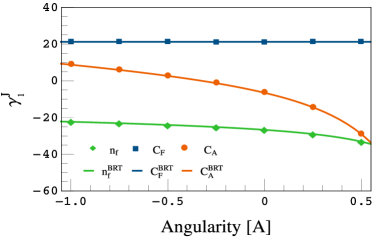
Figure 1: The two-loop non-cusp anomalous dimensions (left) are compared against the semi-analytic results (BRT) of [1]. The new $c_{2}^{J}$ coefficients (right) are obtained for different angularity values. The numerical uncertainties are too small to be visible on the plot.

3 Beam functions

The beam functions are defined via proton matrix elements of collinear field operators. In contrast to the jet functions discussed above, the beam functions are non-perturbative objects, which must be matched onto parton distribution functions (PDF) to extract the perturbative information. At the partonic level, the quark-to-quark beam function is defined e.g. as

$$\frac{1}{2}\,\left[\frac{{\not{n}}}{2}\right]_{\beta\alpha}{\cal B}_{qq}(x,\tau,\mu)=\sum_{X}\delta\Big{(}(1-x)P_{-}-\sum_{i}k_{i}^{-}\Big{)}\,\bra{P}\bar{\chi}_{\alpha}\ket{X}\bra{X}\chi_{\beta}\ket{P}{\cal M}(\tau;\{k_{i}\})\,,$$ (15)

where $\ket{P}$ is now a partonic state with momentum $P^{\mu}$. In the general case, the matching onto the partonic PDF $f_{ij}$ then takes the form,

$${\cal B}_{ij}(x,\tau,\mu) =\sum_{k}\int_{x}^{1}\frac{dz}{z}\,{\cal I}_{ik}\Big{(}\frac{x}{z},\tau,\mu\Big{)}~{}f_{kj}(z,\mu)\,.$$ (16)

While we use the same notation for the Laplace-space measurement function ${\cal M}(\tau;\{k_{i}\})$ as in the previous section, the beam functions ${\cal B}_{ij}$ and the matching kernels ${\cal I}_{ij}$ are distribution-valued in the momentum fraction $x$. To avoid this, we perform an additional Mellin transformation, and we denote the corresponding quantities in Mellin space by $\widehat{\cal B}_{ij}$ and $\widehat{\cal I}_{ij}$. In Mellin space, the bare quantities have a similar perturbative expansion as the jet functions in (3).

3.1 Calculational details

The collinear matrix elements in the definition of the beam functions can be extracted from the well-known splitting functions using crossing symmetry. Notice that at NNLO, the calculation of the beam functions only involves a two-body phase space, for which we employ similar parametrisations as in the jet-function case discussed above. In the following, we focus on the quark-to-quark beam function for transverse momentum resummation, which is defined in SCET-2, and as such requires an additional rapidity regulator. To this end, we adopt the analytic regulator from [18] in a symmetrised version (see also [1, 2, 3]), and we follow the collinear anomaly approach [19] to extract the final matching kernels. Specifically, we write the product of soft and beam-function kernels in Mellin space $(N_{1},N_{2})$ in the form

$$\left[{\cal S}(\tau,\mu,\nu)\;\widehat{\cal I}_{qq}(N_{1},\tau,\mu,\nu)\;\widehat{\cal I}_{\bar{q}\bar{q}}(N_{2},\tau,\mu,\nu)\right]_{q^{2}}\stackrel{{\scriptstyle\alpha=0}}{{\equiv}}\left(\bar{\tau}^{2}q^{2}\right)^{-F_{q\bar{q}}(\tau,\mu)}\;\widehat{I}_{qq}(N_{1},\tau,\mu)\;\widehat{I}_{\bar{q}\bar{q}}(N_{2},\tau,\mu)\,,$$ (17)

where $\alpha$ is the rapidity regulator, $\nu$ is the rapidity scale and $q^{2}$ refers to the hard scale in the problem, e.g. the invariant mass of the Drell-Yan pair. On the right-hand-side of (17), the large rapidity logarithms are then resummed to all orders through the anomaly coefficient $F_{q\bar{q}}(\tau,\mu)$. Due to our specific choice of the rapidity regulator, the collinear and anti-collinear matching kernels on the left-hand-side are furthermore symmetric under the exchange of $n^{\mu}\leftrightarrow\bar{n}^{\mu}$, and it is therefore sufficient to compute only one of them explicitly. On the other hand, we also need the soft function in the same regularisation scheme, for which we rely on SoftSERVE [1, 2, 3].

The renormalised anomaly coefficient then satisfies the RGE

$$\frac{d}{d\ln\mu}\;F_{q\bar{q}}(\tau,\mu)=2\,\Gamma_{\rm cusp}(\alpha_{s})\,,$$ (18)

whose solution, up to two loops, takes the form

$$F_{q\bar{q}}(\tau,\mu)=a_{s}(\mu)\,\Big{\{}2\Gamma_{0}L+d_{1}\Big{\}}+a_{s}^{2}(\mu)\,\Big{\{}2\beta_{0}\Gamma_{0}L^{2}+2\,(\Gamma_{1}+\beta_{0}d_{1})\,L+d_{2}\,\Big{\}}$$ (19)

where $L=\ln(\mu\bar{\tau})$ and $d_{i}$ are the non-logarithmic terms of the renormalised anomaly coefficient. The matching kernels, on the other hand, obey the following RGE in Mellin space,

$$\frac{d}{d\ln\mu}\;\widehat{I}_{qq}(N,\tau,\mu)=2\left[\Gamma_{\rm cusp}(\alpha_{s})\,L+\gamma^{B}(\alpha_{s})\right]\widehat{I}_{qq}(N,\tau,\mu)-2\sum_{j}\;\widehat{I}_{qj}(N,\tau,\mu)\,\widehat{P}_{jq}(N,\mu)\,,$$ (20)

where $\gamma^{B}$ is the non-cusp anomalous dimension, and the sum in the last term of the right-hand-side runs over all partons. In this notation, $\widehat{P}_{qq}$ ($\widehat{P}_{gq}$) is simply the Mellin-transformed splitting function $P_{q\to qg^{*}}$ ($P_{q\to gq^{*}}$). From the solution of (20), we finally extract the non-logarithmic pieces $\textstyle\widehat{I}_{qq,i}(N)$ by expanding in $a_{s}(\mu)$ and setting $\mu=1/\bar{\tau}$, similar to (13).

3.2 Results

At NNLO we have calculated all contributions except for the $C_{F}C_{A}$ colour structure appearing in the $P_{q\to ggq^{*}}$ splitting kernel.

	Analytic	This work
$\gamma_{1}^{n_{f}}$	$-11.395$	$-11.392(8)$
$\gamma_{1}^{C_{F}}$	$10.610$	$10.594(40)$

	Analytic	This work
$d_{2}^{n_{f}}$	$4.148$	$4.147(4)$
$d_{2}^{C_{F}}$	$0$	$0.024(45)$

Table 2: Two-loop non-cusp anomalous dimension (left) and anomaly coefficient (right) for $p_{T}$-resummation. The analytic results have been extracted from [20, 21].

As can be seen in Table 2, our results for the remaining colour structures of the anomaly coefficient $d_{2}$ as well as the non-cusp anomalous dimension $\gamma_{1}^{B}$ are consistent within numerical uncertainties with the analytic results from [20, 21]. In Figure 2, we display the non-logarithmic contribution to the renormalised matching kernel $\textstyle\widehat{I}_{qq,2}(N)$ as a function of the Mellin parameter $N$. For both colour structures computed so far, we again find a very good agreement with the known analytic results.

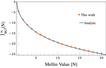
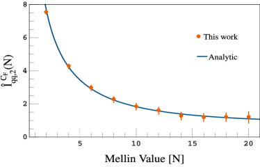
Figure 2: Comparison of the two-loop non-logarithmic contribution to the quark-to-quark matching kernel for $p_{T}$ resummation against the analytic results of [20, 21].

4 Conclusions

We have presented a formalism to automate the calculation of two-loop jet and beam functions. Due to the complicated divergence structure of the underlying collinear matrix elements, we encountered many overlapping singularities in the RR contribution, which we disentangled with the help of a mixed strategy based on sector decomposition, non-linear transformations and selector functions. We furthermore validated our setup against known results for the thrust jet function and the transverse-momentum-dependent beam function, and we obtained a new prediction for the angularity jet function. While we have not yet finished the implementation of the RR contribution in the beam-function case, we plan to look into more observables soon. In the longer term, we also envisage to provide a public code for the calculation of jet and beam functions, similar to the SoftSERVE distribution.

Funding information

This research was supported by the Deutsche Forschungsgemeinschaft (DFG, German Research Foundation) under grant 396021762 - TRR 257.

References

- [1] G. Bell, R. Rahn and J. Talbert, Two-loop anomalous dimensions of generic dijet soft functions, Nucl. Phys. B 936, 520 (2018), 10.1016/j.nuclphysb.2018.09.026, 1805.12414.
- [2] G. Bell, R. Rahn and J. Talbert, Generic dijet soft functions at two-loop order: correlated emissions, JHEP 07, 101 (2019), 10.1007/JHEP07(2019)101, 1812.08690.
- [3] G. Bell, R. Rahn and J. Talbert, Generic dijet soft functions at two-loop order: uncorrelated emissions, JHEP 09, 015 (2020), 10.1007/JHEP09(2020)015, 2004.08396.
- [4] G. Bell, B. Dehnadi, T. Mohrmann and R. Rahn, Automated Calculation of N-jet Soft Functions, PoS LL2018, 044 (2018), 10.22323/1.303.0044, 1808.07427.
- [5] K. Brune, NLO calculation of jet and beam functions in Soft-Collinear Effective Theory, Master’s thesis, Universität Siegen (2019).
- [6] A. Basdew-Sharma, F. Herzog, S. Schrijnder van Velzen and W. J. Waalewijn, One-loop jet functions by geometric subtraction, JHEP 10, 118 (2020), 10.1007/JHEP10(2020)118, 2006.14627.
- [7] G. Altarelli and G. Parisi, Asymptotic Freedom in Parton Language, Nucl. Phys. B 126, 298 (1977), 10.1016/0550-3213(77)90384-4.
- [8] Z. Bern and G. Chalmers, Factorization in one loop gauge theory, Nucl. Phys. B 447, 465 (1995), 10.1016/0550-3213(95)00226-I, hep-ph/9503236.
- [9] Z. Bern, V. Del Duca, W. B. Kilgore and C. R. Schmidt, The infrared behavior of one loop QCD amplitudes at next-to-next-to leading order, Phys. Rev. D 60, 116001 (1999), 10.1103/PhysRevD.60.116001, hep-ph/9903516.
- [10] D. A. Kosower and P. Uwer, One loop splitting amplitudes in gauge theory, Nucl. Phys. B 563, 477 (1999), 10.1016/S0550-3213(99)00583-0, hep-ph/9903515.
- [11] J. M. Campbell and E. W. N. Glover, Double unresolved approximations to multiparton scattering amplitudes, Nucl. Phys. B 527, 264 (1998), 10.1016/S0550-3213(98)00295-8, hep-ph/9710255.
- [12] S. Catani and M. Grazzini, Collinear factorization and splitting functions for next-to-next-to-leading order QCD calculations, Phys. Lett. B 446, 143 (1999), 10.1016/S0370-2693(98)01513-5, hep-ph/9810389.
- [13] S. Catani and M. Grazzini, Infrared factorization of tree level QCD amplitudes at the next-to-next-to-leading order and beyond, Nucl. Phys. B 570, 287 (2000), 10.1016/S0550-3213(99)00778-6, hep-ph/9908523.
- [14] G. Bell, K. Brune, G. Das and M. Wald, to appear .
- [15] S. Borowka, G. Heinrich, S. Jahn, S. P. Jones, M. Kerner, J. Schlenk and T. Zirke, pySecDec: a toolbox for the numerical evaluation of multi-scale integrals, Comput. Phys. Commun. 222, 313 (2018), 10.1016/j.cpc.2017.09.015, 1703.09692.
- [16] T. Becher and M. Neubert, Toward a NNLO calculation of the decay rate with a cut on photon energy. II. Two-loop result for the jet function, Phys. Lett. B 637, 251 (2006), 10.1016/j.physletb.2006.04.046, hep-ph/0603140.
- [17] G. Bell, A. Hornig, C. Lee and J. Talbert, angularity distributions at NNLL′ accuracy, JHEP 01, 147 (2019), 10.1007/JHEP01(2019)147, 1808.07867.
- [18] T. Becher and G. Bell, Analytic Regularization in Soft-Collinear Effective Theory, Phys. Lett. B 713, 41 (2012), 10.1016/j.physletb.2012.05.016, 1112.3907.
- [19] T. Becher and M. Neubert, Drell-Yan Production at Small , Transverse Parton Distributions and the Collinear Anomaly, Eur. Phys. J. C 71, 1665 (2011), 10.1140/epjc/s10052-011-1665-7, 1007.4005.
- [20] T. Gehrmann, T. Luebbert and L. L. Yang, Transverse parton distribution functions at next-to-next-to-leading order: the quark-to-quark case, Phys. Rev. Lett. 109, 242003 (2012), 10.1103/PhysRevLett.109.242003, 1209.0682.
- [21] T. Gehrmann, T. Luebbert and L. L. Yang, Calculation of the transverse parton distribution functions at next-to-next-to-leading order, JHEP 06, 155 (2014), 10.1007/JHEP06(2014)155, 1403.6451.