Automated Calculation of ${\boldsymbol{N}}$-jet Soft Functions

Abstract:

We present a systematic framework for the calculation of soft functions that are defined in terms of $N\geq 2$ light-like Wilson lines. The formalism represents an extension of a method that we developed earlier for the calculation of dijet soft functions to the general $N$-jet case. We discuss the technical aspects of this generalisation, focussing on SCET-1 soft functions that obey the non-Abelian exponentiation theorem in this contribution. As a first application of our method, we consider the $N$-jettiness observable and present numerical results for the $1$-jettiness and $2$-jettiness hadron-collider soft functions to next-to-next-to-leading order in the perturbative expansion.

1 Introduction

Soft functions are essential ingredients of factorisation theorems that arise whenever the QCD radiation to a hard-scattering process is restricted to the soft and collinear regions. Factorisation is the basis for an all-order resummation of logarithmic corrections, which can be achieved e.g. by solving renormalisation group (RG) equations in Soft-Collinear Effective Theory (SCET) [1, 2, 3]. In the past years, the factorised cross sections have also been used as a subtraction (or slicing) technique for fixed-order QCD calculations, with the $q_{T}$ subtraction [4] and the $N$-jettiness subtraction [5, 6] being the most prominent examples.

In this contribution we present a generalisation of a method that we developed previously for the calculation of soft functions that are defined in terms of two back-to-back light-like Wilson lines [7, 8, 9]. As a first step to the general $N$-jet case, we focus in this work on SCET-1 soft functions that obey the non-Abelian exponentiation (NAE) theorem [10, 11]. In the following, we discuss the technical aspects of our approach, and present numerical results for the $N$-jettiness soft function to next-to-next-to-leading order (NNLO) in the perturbative expansion.

2 $\boldsymbol{N}$-jet soft functions

We consider soft functions of the generic form

$$S(\tau,\mu)=\sum_{X}\;\mathcal{M}(\tau;\{k_{i}\})\;\langle 0|\big{(}S_{n_{1}}S_{n_{2}}\cdots S_{n_{N}}\big{)}^{\dagger}|X\rangle\langle X|S_{n_{1}}S_{n_{2}}\cdots S_{n_{N}}|0\rangle\,,$$ (1)

where $S_{n_{i}}$ are soft Wilson lines extending along $N\geq 2$ light-like directions $n_{i}^{\mu}$. The Wilson lines depend on the colour representation of the associated hard partons, and the soft function itself is a matrix in colour space. The path of the Wilson lines – and hence the $i\epsilon$ prescription of the eikonal propagators – furthermore differs for incoming and outgoing partons. The term $\mathcal{M}(\tau;\{k_{i}\})$ represents a generic measurement function that provides a constraint on the soft radiation with momenta $\{k_{i}\}$. The specific form we assume for the measurement function will be given in the following sections, but we generally assume that it is defined in Laplace space with $\tau$ denoting the corresponding Laplace variable.

Assuming that the tree-level (no emission) measurement function is normalised to one, the perturbative expansion of the $N$-jet soft function can be written in the form

$$S(\tau,\mu)=1+\left(\frac{Z_{\alpha}\alpha_{s}}{4\pi}\right)(\mu^{2}\bar{\tau}^{2})^{\epsilon}\;S^{(1)}(\epsilon)+\left(\frac{Z_{\alpha}\alpha_{s}}{4\pi}\right)^{2}(\mu^{2}\bar{\tau}^{2})^{2\epsilon}\;S^{(2)}(\epsilon)+\mathcal{O}(\alpha_{s}^{3})\,,$$ (2)

where $\epsilon=(4-d)/2$ is the dimensional regulator, $\bar{\tau}=\tau e^{\gamma_{E}}$ and $\alpha_{s}$ is the $\overline{\textrm{MS}}$-renormalised coupling constant, which is related to the bare coupling constant $\alpha_{s}^{0}$ via $Z_{\alpha}\alpha_{s}\,\mu^{2\epsilon}=e^{-\epsilon\gamma_{E}}(4\pi)^{\epsilon}\alpha_{s}^{0}$ with $Z_{\alpha}=1-\beta_{0}\alpha_{s}/(4\pi\epsilon)$ and $\beta_{0}=11/3\,C_{A}-4/3\,T_{F}n_{f}$. In this notation, the first term represents the unit operator in colour space, whereas the NLO and NNLO coefficients $S^{(1,2)}(\epsilon)$ have a non-trivial colour structure, and they implicitly depend on the kinematic factors $n_{ij}\equiv n_{i}\cdot n_{j}$. Our strategy for computing these coefficients closely follows the one we adopted for the calculation of dijet soft functions in [7]. In particular, we assume in this work that the soft functions are not sensitive to rapidity divergences (and are therefore of SCET-1 type) and that they are consistent with NAE.

3 NLO calculation

At NLO the virtual corrections are scaleless and vanish in dimensional regularisation. The real-emission diagrams that connect the same Wilson line also vanish, since the reference vectors $n_{i}^{\mu}$ are all light-like. We are thus left at this order with real-emission diagrams that connect a pair of different Wilson lines, and the soft function is thus given by a sum over dipole contributions,

$$S^{(1)}(\epsilon)=\sum_{i\neq j}\,{\mathbf{T}}_{i}\cdot{\mathbf{T}}_{j}\,\Big{(}\frac{n_{ij}}{2}\Big{)}^{\epsilon}\,S_{ij}^{(1)}(\epsilon)\,,$$ (3)

where ${\mathbf{T}}_{i}$ and ${\mathbf{T}}_{j}$ are the colour generators of the $i$’th and $j$’th parton in the colour-space notation of [12]. The dipole contributions can be calculated in close analogy to the method we developed for dijet soft functions in [7]. We thus start from

$$S_{ij}^{(1)}(\epsilon)=-\frac{(2\pi\,n_{ij}\,e^{\gamma_{E}}\tau^{2})^{-\epsilon}}{(2\pi)^{d-1}}\,\int d^{d}k\;\,\delta(k^{2})\,\theta(k^{0})\,\mathcal{M}_{1}(\tau;k)\,|\mathcal{A}_{ij}(k)|^{2}\,,$$ (4)

where $|\mathcal{A}_{ij}(k)|^{2}=16\pi^{2}n_{ij}/k_{i}k_{j}$ is the square of the dipole matrix element with $k_{i}=k\cdot n_{i}$ and $k_{j}=k\cdot n_{j}$. We furthermore decompose the gluon momentum according to

$$k^{\mu}=k_{j}\,\frac{n_{i}^{\mu}}{n_{ij}}+\,k_{i}\,\frac{n_{j}^{\mu}}{n_{ij}}+k_{\perp}^{\mu}\,,$$ (5)

where $k_{\perp}^{\mu}$ is a vector that is transverse to the jet directions $n_{i}^{\mu}$ and $n_{j}^{\mu}$. In $d$ dimensions the transverse space can be parametrised by $(d-2)$ components, and we find it convenient to work in a frame in which the dipole jets are back-to-back, such that the transverse space is purely space-like and can be expressed using ordinary spherical coordinates. We further introduce the boost-invariant variables $k_{T}=\sqrt{2k_{i}k_{j}/n_{ij}}$ and $y=k_{i}/k_{j}$, and write the one-emission measurement function as

$$\mathcal{M}_{1}(\tau;k)=\exp\bigg{\{}-\tau\,\sqrt{\frac{n_{ij}}{2}}\,k_{T}\bigg{(}y^{n/2}\,f_{A}(y,\theta_{1},\theta_{2})\,\theta(1-y)+y^{-n/2}\,f_{B}(1/y,\theta_{1},\theta_{2})\,\theta(y-1)\bigg{)}\bigg{\}}\,,$$ (6)

which consists of two hemisphere contributions for $y\leq 1$ and $y\geq 1$. In the first term, we factor out an appropriate power of the rapidity variable $y$ to make sure that the function $f_{A}(y,\theta_{1},\theta_{2})$ is finite and non-zero in the limit $y\to 0$, and we do so similarly for the second term for $y\to\infty$ [7]. The exponential typically arises from a Laplace transformation, and we assume that the Laplace variable $\tau$ has dimension $1/$mass, which fixes the linear dependence on $k_{T}$ on dimensional grounds. We further account for two angular dependences, since the projection of the gluon momentum onto the jet directions $n_{k}^{\mu}$ can in general be expressed in terms of two angles in the transverse plane [13].

After performing the observable-independent integrations and mapping $y\to 1/y$ in the second hemisphere contribution, we obtain the following representation of the NLO dipole contribution,

$$S_{ij}^{(1)}(\epsilon) =\frac{2\,e^{-\gamma_{E}\epsilon}}{\pi}\,\frac{\Gamma(-2\epsilon)}{\Gamma(-\epsilon)}\;\int_{0}^{1}dy\;\,y^{-1+n\epsilon}\;\int_{-1}^{1}d\cos\theta_{1}\;\,\sin^{-1-2\epsilon}\theta_{1}$$

$$\qquad\quad\int_{-1}^{1}d\cos\theta_{2}\;\,\sin^{-2-2\epsilon}\theta_{2}\;\;\Big{\{}f_{A}(y,\theta_{1},\theta_{2})^{2\epsilon}+f_{B}(y,\theta_{1},\theta_{2})^{2\epsilon}\Big{\}}\,.$$ (7)

Notice that for SCET-1 soft functions with $n\neq 0$, the rapidity integral produces a pole in $\epsilon$ in the collinear limit $y\to 0$. The factor $\Gamma(-2\epsilon)$ furthermore captures a soft singularity that arises in the limit $k_{T}\to 0$. We also remark that the integration over the angle $\theta_{2}$ produces an unphysical (spurious) divergence, which is compensated by the prefactor $1/\Gamma(-\epsilon)\sim\mathcal{O}(\epsilon)$. Our result in (3) generalises the corresponding expression for dijet soft functions in [7], where we assumed that the two jets are back-to-back and that the observable is symmetric under $n\leftrightarrow\bar{n}$ exchange.

4 NNLO calculation

At NNLO the two-loop virtual corrections are again scaleless and vanish. The remaining contributions are the mixed real-virtual (RV) and double real-emission corrections. The latter consists of two contributions: the emission of a soft quark-antiquark pair ($q\bar{q}$) and the emission of two soft gluons ($gg$). Hence the total NNLO correction to the soft function can be written in the form

$$S^{(2)}(\epsilon)=S^{(2,{\rm RV})}(\epsilon)+{S}^{(2,q\bar{q})}(\epsilon)+{S}^{(2,gg)}(\epsilon)\,.$$ (8)

The real-virtual correction consists of two-particle and three-particle correlations [14],

$$S^{(2,{\rm RV})}(\epsilon)=C_{A}\,\sum_{i\neq j}\,{\mathbf{T}}_{i}\cdot{\mathbf{T}}_{j}\,\Big{(}\frac{n_{ij}}{2}\Big{)}^{2\epsilon}\,S_{ij}^{(2,{\rm Re})}(\epsilon)+\sum_{i\neq j\neq k}(\lambda_{ij}-\lambda_{ip}-\lambda_{jp})\,f_{ABC}\;{\mathbf{T}}_{i}^{A}\;{\mathbf{T}}_{j}^{B}\;{\mathbf{T}}_{k}^{C}\;S_{ijk}^{(2,{\rm Im})}(\epsilon)\,,$$ (9)

where $\lambda_{AB}=1$ if partons $A$ and $B$ are both incoming or outgoing, and $\lambda_{AB}=0$ otherwise. Here the indices $i,j,k$ refer to the hard partons associated with the respective Wilson lines and $p$ represents the emitted soft gluon. The first term again has a dipole structure and the corresponding matrix element is proportional to $(n_{ij}/2k_{i}k_{j})^{1+\epsilon}$. The second term reveals a three-parton colour correlation, which we will refer to as a tripole contribution. It arises from the imaginary part of the loop integral, and it is thus process dependent. In processes with three hard partons, one can show that the tripole contribution vanishes because of colour conservation [14], but for general processes with four or more partons it leads to a non-trivial correction. The corresponding matrix element is of the form $(n_{ij}/2k_{i}k_{j})^{\epsilon}(n_{ik}/2k_{i}k_{k})$. As both matrix elements resemble the one of the NLO calculation, we apply a similar phase-space parametrisation to factorise the divergences.

For the double real-emission contribution, we obtain [15]

$${S}^{(2,q\bar{q})}(\epsilon) =T_{F}\,n_{f}\,\sum_{i\neq j}\,{\mathbf{T}}_{i}\cdot{\mathbf{T}}_{j}\,\Big{(}\frac{n_{ij}}{2}\Big{)}^{2\epsilon}S_{ij}^{(2,q\bar{q})}(\epsilon)\,,$$ (10)

$${S}^{(2,gg)}(\epsilon) =C_{A}\,\sum_{i\neq j}\,{\mathbf{T}}_{i}\cdot{\mathbf{T}}_{j}\,\Big{(}\frac{n_{ij}}{2}\Big{)}^{2\epsilon}S_{ij}^{(2,gg)}(\epsilon)+\frac{1}{4}\,\sum_{i\neq j}\sum_{k\neq l}\big{\{}{\mathbf{T}}_{i}\cdot{\mathbf{T}}_{j}\,,\,{\mathbf{T}}_{k}\cdot{\mathbf{T}}_{l}\big{\}}\Big{(}\frac{n_{ij}\,n_{kl}}{4}\Big{)}^{\epsilon}S_{ij}^{(1)}(\epsilon)\,S_{kl}^{(1)}(\epsilon),$$

where in the last term we asumed that the observable is consistent with NAE, and

$$S_{ij}^{(2,X)}(\epsilon)=-\frac{(2\pi\,n_{ij}\,e^{\gamma_{E}}\tau^{2})^{-2\epsilon}}{(2\pi)^{2d-2}}\,\int d^{d}k\;\,\delta(k^{2})\,\theta(k^{0})\,\int d^{d}l\;\,\delta(l^{2})\,\theta(l^{0})\;\mathcal{M}_{2}(\tau;k,l)\,|\mathcal{A}_{ij}^{X}(k,l)|^{2}$$ (11)

for $X\in\{q\bar{q},gg\}$. The corresponding matrix elements for both colour structures $|\mathcal{A}_{ij}^{X}(k,l)|^{2}$ can be found in [15]. Unlike the single-emission case, the double real-emission correction exhibits overlapping divergences, which we disentangle with a suitable phase-space reparametrisation [16].

For the double real-emission contribution, we again follow [7] and introduce the variables

$$p_{T}=\sqrt{\frac{2(k_{i}+l_{i})(k_{j}+l_{j})}{n_{ij}}}\,,\qquad y=\frac{k_{i}+l_{i}}{k_{j}+l_{j}}\,,\qquad a=\sqrt{\frac{k_{j}\,l_{i}}{k_{i}\,l_{j}}}\,,\qquad b=\sqrt{\frac{k_{i}\,k_{j}}{l_{i}\,l_{j}}}\,.$$ (12)

In terms of these variables, our ansatz for the two-emission measurement function becomes

$$\mathcal{M}_{2}(\tau;k,l) =\exp\bigg{\{}-\tau\,\sqrt{\frac{n_{ij}}{2}}\,p_{T}\,\theta(1-a)$$ (13)

$$\quad\times\bigg{(}y^{n/2}\Big{[}F_{A}\big{(}a,b,y,\{\theta_{i}\}\big{)}\,\theta(1-b)+F_{B}\big{(}a,1/b,y,\{\theta_{i}\}\big{)}\,\theta(b-1)\Big{]}\theta(1-y)$$

$$\qquad+y^{-n/2}\Big{[}F_{C}\big{(}a,b,1/y,\{\theta_{i}\}\big{)}\theta(1-b)+F_{D}\big{(}a,1/b,1/y,\{\theta_{i}\}\big{)}\theta(b-1)\Big{]}\theta(y-1)\bigg{)}\bigg{\}},$$

where $\{\theta_{i}\}\equiv\{\theta_{k_{1}},\theta_{k_{2}},\theta_{k_{3}},\theta_{l_{1}},\theta_{l_{2}}\}$ represents a set of angles that we use to express the momenta of the two emitted partons in the transverse space [13]. Furthermore, similar to the single-emission case in (6), we have factorised the linear dependence on $p_{T}$ on dimensional grounds, as well as the asymptotic behaviour of the measurement function in the limits $y\to 0$ and $y\to\infty$. We further exploit the symmetry under $k\leftrightarrow l$ exchange, to map the contribution from $a\geq 1$ onto $a\leq 1$. The functions $F_{i}$ satisfy certain constraints from infrared and collinear safety, which we discussed in detail for the dijet case in [9]. With the phase-space parametrisation and the measurement function at hand, one can then derive a similar master formula for the double real-emission contribution as in the NLO case, in which all singularities are factorised. Further details will be given in [13].

5 Renormalisation

In Laplace space the relation between the bare and the renormalised soft function reads

$$S_{0}(\tau)=Z_{S}(\tau,\mu)\;S(\tau,\mu)\;Z_{S}^{\dagger}(\tau,\mu)\,,$$ (14)

where the counterterm $Z_{S}(\tau,\mu)$ is a matrix in colour space. The $\overline{\text{MS}}$ renormalised soft function satisfies the RG equation

$$\frac{\mathrm{d}}{\mathrm{d}\ln\mu}\;S(\tau,\mu)=\frac{1}{2}\,\Gamma_{S}(\tau,\mu)\,S(\tau,\mu)+\frac{1}{2}\,S(\tau,\mu)\,\Gamma_{S}(\tau,\mu)^{\dagger}$$ (15)

with anomalous dimension

$$\Gamma_{S}(\tau,\mu)=\frac{1}{n}\,\bigg{\{}\sum_{i\neq j}\,{\mathbf{T}}_{i}\cdot{\mathbf{T}}_{j}\;\Gamma_{\rm cusp}(\alpha_{s})\bigg{[}2\,\ln\bigg{(}\sqrt{\frac{n_{ij}}{2}}\,\mu\bar{\tau}\bigg{)}-i\pi\,\lambda_{ij}\bigg{]}+2\gamma^{S}(\alpha_{s})\bigg{\}}\,,$$ (16)

where $\lambda_{ij}$ has been defined after (9). The imaginary part is related to the anomalous dimension of the associated hard function in the factorisation theorem, whose general structure was discussed in [17]. The cusp anomalous dimension has a perturbative expansion $\Gamma_{\rm cusp}(\alpha_{s})=\sum_{n=0}^{\infty}\Gamma_{n}(\frac{\alpha_{s}}{4\pi})^{n+1}$, with leading coefficients $\Gamma_{0}=4$ and $\Gamma_{1}=(268/9-4\pi^{2}/3)C_{A}-80/9\,T_{F}n_{f}$. Up to the considered two-loop order, the soft anomalous dimension also has a dipole structure and can be written in the form $\gamma^{S}(\alpha_{s})=\sum_{i\neq j}\,{\mathbf{T}}_{i}\cdot{\mathbf{T}}_{j}\,\big{\{}\gamma^{(0)}_{ij}\,(\frac{\alpha_{s}}{4\pi})+\gamma^{(1)}_{ij}\,(\frac{\alpha_{s}}{4\pi})^{2}\big{\}}$. Following [7, 9], we find it furthermore convenient to define the anomalous dimensions with a common prefactor $1/n$, where $n$ is related to the asymptotic behaviour of the observable in the collinear limit, see (6) and (13).

The two-loop solution of the RG equation takes the form

$$S(\tau,\mu) =1+\left(\frac{\alpha_{s}}{4\pi}\right)\sum_{i\neq j}\,{\mathbf{T}}_{i}\cdot{\mathbf{T}}_{j}\,\bigg{(}\frac{\Gamma_{0}}{n}\,L_{ij}^{2}+\frac{2\gamma^{(0)}_{ij}}{n}\,L_{ij}+c_{ij}^{(1)}\bigg{)}+\left(\frac{\alpha_{s}}{4\pi}\right)^{2}$$ (17)

$$\times\bigg{\{}\sum_{i\neq j}\,{\mathbf{T}}_{i}\cdot{\mathbf{T}}_{j}\,\bigg{(}\frac{2\beta_{0}\Gamma_{0}}{3n}\,L_{ij}^{3}+\bigg{(}\frac{\Gamma_{1}}{n}+\frac{2\beta_{0}\gamma^{(0)}_{ij}}{n}\bigg{)}L_{ij}^{2}+2\bigg{(}\frac{\gamma^{(1)}_{ij}}{n}+\beta_{0}c_{ij}^{(1)}\bigg{)}L_{ij}+c_{ij}^{(2)}\bigg{)}$$

$$\hskip 19.91692pt-2\pi\sum_{i\neq j\neq k}f_{ABC}\;{\mathbf{T}}_{i}^{A}\;{\mathbf{T}}_{j}^{B}\;{\mathbf{T}}_{k}^{C}\;\bigg{(}\frac{\lambda_{ij}\Gamma_{0}}{n^{2}}\bigg{(}\frac{\Gamma_{0}}{3}L_{jk}^{3}+\gamma^{(0)}_{jk}L_{jk}^{2}+n\,c_{jk}^{(1)}L_{jk}\bigg{)}+c_{ijk}^{(2)}\bigg{)}$$

$$\hskip 19.91692pt+\frac{1}{4}\,\sum_{i\neq j}\sum_{k\neq l}\big{\{}{\mathbf{T}}_{i}\cdot{\mathbf{T}}_{j}\,,\,{\mathbf{T}}_{k}\cdot{\mathbf{T}}_{l}\big{\}}\bigg{(}\frac{\Gamma_{0}}{n}\,L_{ij}^{2}+\frac{2\gamma^{(0)}_{ij}}{n}\,L_{ij}+c_{ij}^{(1)}\bigg{)}\bigg{(}\frac{\Gamma_{0}}{n}\,L_{kl}^{2}+\frac{2\gamma^{(0)}_{kl}}{n}\,L_{kl}+c_{kl}^{(1)}\bigg{)}\bigg{\}},$$

where $L_{ij}=\ln\big{(}\sqrt{n_{ij}/2}\,\mu\bar{\tau}\big{)}$ etc. Here the tripole structure arises from commutators of colour generators, e.g. $\big{[}{\mathbf{T}}_{i}\cdot{\mathbf{T}}_{j}\,,\,{\mathbf{T}}_{j}\cdot{\mathbf{T}}_{k}\big{]}=-if_{ABC}\;{\mathbf{T}}_{i}^{A}\;{\mathbf{T}}_{j}^{B}\;{\mathbf{T}}_{k}^{C}$.

The counterterm, on the other hand, fulfills the RG equation

$$\frac{\mathrm{d}}{\mathrm{d}\ln\mu}\;Z_{S}(\tau,\mu)=-\frac{1}{2}\,Z_{S}(\tau,\mu)\,\Gamma_{S}(\tau,\mu)\,,$$ (18)

and its explicit solution to two-loop order is given by

$$Z_{S}(\tau,\mu) =1+\left(\frac{\alpha_{s}}{4\pi}\right)\sum_{i\neq j}\,{\mathbf{T}}_{i}\cdot{\mathbf{T}}_{j}\,\bigg{(}\frac{\Gamma_{0}}{4n}\,\frac{1}{\epsilon^{2}}+\frac{G^{(0)}_{ij}}{4n}\,\frac{1}{\epsilon}\bigg{)}+\left(\frac{\alpha_{s}}{4\pi}\right)^{2}$$ (19)

$$\quad\times\bigg{\{}\sum_{i\neq j}\,{\mathbf{T}}_{i}\cdot{\mathbf{T}}_{j}\,\bigg{(}-\frac{3\beta_{0}\Gamma_{0}}{16n}\,\frac{1}{\epsilon^{3}}+\frac{\Gamma_{1}-2\beta_{0}G^{(0)}_{ij}}{16n}\,\frac{1}{\epsilon^{2}}+\frac{G^{(1)}_{ij}}{8n}\,\frac{1}{\epsilon}\bigg{)}$$

$$\hskip 31.29802pt+\frac{1}{4}\,\sum_{i\neq j}\sum_{k\neq l}\big{\{}{\mathbf{T}}_{i}\cdot{\mathbf{T}}_{j}\,,\,{\mathbf{T}}_{k}\cdot{\mathbf{T}}_{l}\big{\}}\bigg{(}\frac{\Gamma_{0}}{4n}\,\frac{1}{\epsilon^{2}}+\frac{G^{(0)}_{ij}}{4n}\,\frac{1}{\epsilon}\bigg{)}\bigg{(}\frac{\Gamma_{0}}{4n}\,\frac{1}{\epsilon^{2}}+\frac{G^{(0)}_{kl}}{4n}\,\frac{1}{\epsilon}\bigg{)}\bigg{\}},$$

where $G^{(k)}_{ij}=(2L_{ij}-i\pi\lambda_{ij})\Gamma_{k}+2\,\gamma^{(k)}_{ij}$ . Using these expressions, one can reconstruct all divergences of the bare soft function through NNLO via (14).

6 $\boldsymbol{N}$-jettiness soft function

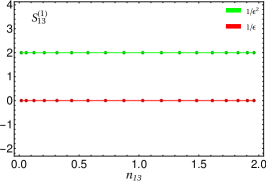
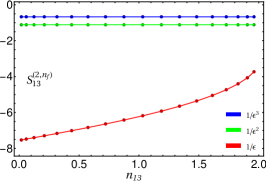
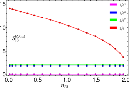
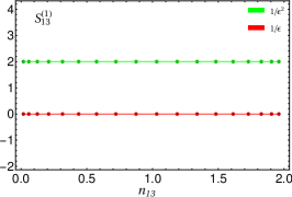
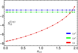
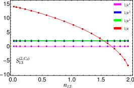
Figure 1: Dipole contributions to the 1-jettiness (upper row) and 2-jettiness (lower row) soft functions. The first, second and third column show the $\mathcal{O}(\alpha_{s})$, $\mathcal{O}(T_{f}\,n_{f}\,\alpha_{s}^{2})$ and $\mathcal{O}(C_{A}\,\alpha_{s}^{2})$ contributions as defined in the text. The dots show our numerical results for the poles of the bare soft function, and the solid lines are the predictions from the RG equation.

As an application of our framework, we consider the $N$-jettiness observable at hadron colliders. $N$-jettiness is defined as [18]

$$\mathcal{T}_{N}=\sum_{k}\;\min_{i}\big{\{}n_{i}\cdot p_{k}\big{\}}\,,$$ (20)

where for simplicity we adopt a specific normalisation that was also used in [19, 20]. Here $p_{k}^{\mu}$ are the momenta of the final-state radiation, and $n_{i}^{\mu}$ are a set of light-like reference vectors, with $i=1,2$ denoting the beam directions and $i=3,\ldots,(N+2)$ refering to the directions of the final-state jets. The $N$-jettiness hadron collider soft function thus corresponds to a $(N+2)$-jet soft function in the terminology of our paper.

The Laplace-space $N$-jettiness soft function falls into the class (1), and it is defined in SCET-1 (with parameter $n=1$) and obeys NAE. We can thus apply the developed formalism to compute the $N$-jettiness soft function for – in principle – arbitrary values of $N$. In the following, we show explicit results for the 1-jettiness and 2-jettiness soft functions. As the 1-jettiness soft function is already known to NNLO [19, 20], we can test our method by comparing our results to these calculations. The 2-jettiness soft function, on the other hand, is currently only known to NLO [21], and our results represent the first NNLO calculation for this observable.

We first illustrate that the divergences of the bare soft function calculation agree with the predictions from the RG equation that we discussed in Section 5. The relevant anomalous dimensions are all known to the considered order, and can be found in [21]. In Figure 1 we show the $(13)$-dipole contribution to the 1-jettiness (upper row) and 2-jettiness (lower row) soft functions for illustration. The plots show the NLO dipole $S_{13}^{(1)}$ (left) and the NNLO dipole contributions $S_{13}^{(2,n_{f})}=S_{13}^{(2,q\bar{q})}$ (middle) and $S_{13}^{(2,C_{A})}=S_{13}^{(2,{\rm Re})}+S_{13}^{(2,gg)}$ (right) as a function of $n_{13}$ . The dots represent the numbers that we obtain by processing the formulae from Sections 3 and 4 through pySecDec [22]. Our predictions use the Vegas integrator provided by the Cuba library [23], and they typically have numerical uncertainties at the subpercent level which are not visible on the scale of the plots. The numbers of the bare soft function calculation are then compared to the predictions of the RG equation, which are illustrated by the solid lines. As can be seen from the plots, the agreement is very satisfactory for all pole coefficients, which similarly holds for the other dipole contributions.

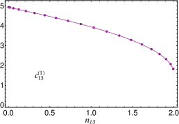
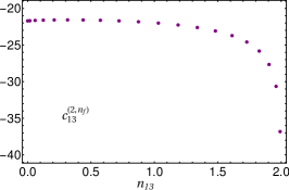
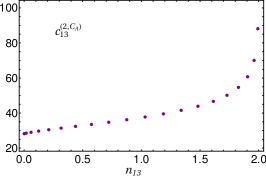
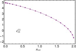
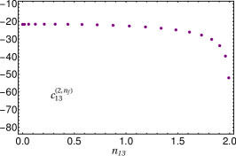
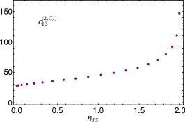
Figure 2: The same as in Figure 1, but for the finite terms of the renormalised soft function. The solid lines in the left plots show the result of the NLO calculation from [21].

In Figure 2 we display the corresponding finite terms of the renormalised soft function as defined in (17). The plots show the NLO coefficient $c_{13}^{(1)}$ (left) and the NNLO colour coefficients defined by $c_{13}^{(2)}=T_{F}\,n_{f}\,c_{13}^{(2,n_{f})}+C_{A}\,c_{13}^{(2,C_{A})}$ (middle and right). Our NLO results can be compared to the calculation in [21], which provides integral representations for the NLO dipoles for an arbitrary number of jets in distribution space. These results can readily be transformed to Laplace space and integrated numerically, which yields the solid lines in the left plots of Figure 2. We again observe a perfect agreement with these predictions for both the 1-jettiness and the 2-jettiness.

Whereas our results for the NNLO 2-jettiness soft function are new, the 1-jettiness results can be compared to the calculations in [19, 20]. To this end, we adopt the conventions used in [20], which provides useful fit functions for the complete NNLO correction for all partonic channels. We thus sum over the dipole contributions shown in Figure 2 with appropriate colour factors, and since the computation in [20] was carried out in distribution space, we transform our results to this space for the comparison. The finite non-logarithmic term at NNLO is proportional to $\delta(\mathcal{T}_{N})$ and denoted with $C_{-1,nab}$ in [20]. Our results for this coefficient are shown in the first panel of Figure 3 for different partonic channels, where the dots represent our numerical pySecDec numbers and the solid lines are the fit functions from [20]. The agreement between the two predictions is another highly non-trivial cross check of our calculation.

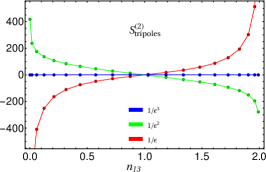
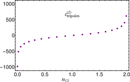
Figure 3: The first panel shows our results for the $\delta(\mathcal{T}_{1})$ coefficient of the renormalised 1-jettiness soft function (dots) in comparison with the fit functions from [20] (solid lines). The second panel compares our prediction for the sum over all tripole contributions to the 2-jettiness soft function (dots) with the one from the RG equation (solid lines). The third panel shows the corresponding finite term of the renormalised soft function.

We finally address the tripole contributions, which give a non-vanishing correction only for processes with four or more hard partons. They thus contribute to the 2-jettiness soft function, and for convenience we present our results for the sum over all tripole contributions in the form

$$\sum_{i\neq j\neq k}(\lambda_{ij}-\lambda_{ip}-\lambda_{jp})\,f_{ABC}\;{\mathbf{T}}_{i}^{A}\;{\mathbf{T}}_{j}^{B}\;{\mathbf{T}}_{k}^{C}\;S_{ijk}^{(2,{\rm Im})}(\epsilon)\equiv f_{ABC}\;{\mathbf{T}}_{1}^{A}\;{\mathbf{T}}_{2}^{B}\;{\mathbf{T}}_{3}^{C}\;S_{\rm tripoles}^{(2)}(\epsilon)\,,$$ (21)

where we have used colour conservation to bring the colour generators into this particular form. Our results for the divergences of the tripole contribution are represented by the dots in the middle panel of Figure 3. They are again in perfect agreement with the predictions from the RG equation, which are indicated by the solid lines. In the right panel of Figure 3, we finally display the corresponding finite term of the renormalised soft function in the form

$$\sum_{i\neq j\neq k}f_{ABC}\;{\mathbf{T}}_{i}^{A}\;{\mathbf{T}}_{j}^{B}\;{\mathbf{T}}_{k}^{C}\;c_{ijk}^{(2)}\equiv f_{ABC}\;{\mathbf{T}}_{1}^{A}\;{\mathbf{T}}_{2}^{B}\;{\mathbf{T}}_{3}^{C}\;c_{\rm tripoles}^{(2)}\,,$$ (22)

which is another new result.

7 Conclusions

We presented a generalisation of a formalism that we developed earlier for the calculation of dijet soft functions in [7, 8, 9]. Our method allows for a systematic computation of NNLO soft function with an arbitrary number of light-like Wilson lines. As a first step to the general $N$-jet case, we focussed on SCET-1 soft functions that obey the NAE theorem.

We then applied the novel formalism to compute the $N$-jettiness soft function for single-jet and dijet production at hadron colliders. We checked that the poles terms of the bare soft functions agree with the predictions from the RG equation, and we compared our NNLO 1-jettiness result with the calculation in [20]. Our prediction for the 2-jettiness soft function is new, and it provides the last missing ingredient to apply the $N$-jettiness subtraction technique to processes with two jets. As our setup is fairly general, we can also compute soft functions for other hadronic event shapes or boosted top observables with the same techniques. Further details will be given in [13].

- [1] C. W. Bauer, S. Fleming, D. Pirjol and I. W. Stewart, An Effective field theory for collinear and soft gluons: Heavy to light decays, Phys. Rev. D63 (2001) 114020 [hep-ph/0011336].
- [2] C. W. Bauer, D. Pirjol and I. W. Stewart, Soft collinear factorization in effective field theory, Phys. Rev. D65 (2002) 054022 [hep-ph/0109045].
- [3] M. Beneke, A. P. Chapovsky, M. Diehl and T. Feldmann, Soft collinear effective theory and heavy to light currents beyond leading power, Nucl. Phys. B643 (2002) 431 [hep-ph/0206152].
- [4] S. Catani and M. Grazzini, An NNLO subtraction formalism in hadron collisions and its application to Higgs boson production at the LHC, Phys. Rev. Lett. 98 (2007) 222002 [hep-ph/0703012].
- [5] R. Boughezal, C. Focke, X. Liu and F. Petriello, -boson production in association with a jet at next-to-next-to-leading order in perturbative QCD, Phys. Rev. Lett. 115 (2015) 062002 [1504.02131].
- [6] J. Gaunt, M. Stahlhofen, F. J. Tackmann and J. R. Walsh, N-jettiness Subtractions for NNLO QCD Calculations, JHEP 09 (2015) 058 [1505.04794].
- [7] G. Bell, R. Rahn and J. Talbert, Automated Calculation of Dijet Soft Functions in Soft-Collinear Effective Theory, PoS RADCOR2015 (2016) 052 [1512.06100].
- [8] G. Bell, R. Rahn and J. Talbert, Automated Calculation of Dijet Soft Functions in the Presence of Jet Clustering Effects, PoS RADCOR2017 (2018) 047 [1801.04877].
- [9] G. Bell, R. Rahn and J. Talbert, Two-loop anomalous dimensions of generic dijet soft functions, 1805.12414.
- [10] J. G. M. Gatheral, Exponentiation of Eikonal Cross-sections in Nonabelian Gauge Theories, Phys. Lett. 133B (1983) 90.
- [11] J. Frenkel and J. C. Taylor, Nonabelian eikonal exponentiation, Nucl. Phys. B246 (1984) 231.
- [12] S. Catani and M. H. Seymour, A General algorithm for calculating jet cross-sections in NLO QCD, Nucl. Phys. B485 (1997) 291 [hep-ph/9605323].
- [13] G. Bell, B. Dehnadi, T. Mohrmann and R. Rahn. In preparation.
- [14] S. Catani and M. Grazzini, The soft gluon current at one loop order, Nucl. Phys. B591 (2000) 435 [hep-ph/0007142].
- [15] S. Catani and M. Grazzini, Infrared factorization of tree level QCD amplitudes at the next-to-next-to-leading order and beyond, Nucl. Phys. B570 (2000) 287 [hep-ph/9908523].
- [16] G. Bell, R. Rahn and J. Talbert. In preparation.
- [17] T. Becher and M. Neubert, On the Structure of Infrared Singularities of Gauge-Theory Amplitudes, JHEP 06 (2009) 081 [0903.1126].
- [18] I. W. Stewart, F. J. Tackmann and W. J. Waalewijn, N-Jettiness: An Inclusive Event Shape to Veto Jets, Phys. Rev. Lett. 105 (2010) 092002 [1004.2489].
- [19] R. Boughezal, X. Liu and F. Petriello, -jettiness soft function at next-to-next-to-leading order, Phys. Rev. D91 (2015) 094035 [1504.02540].
- [20] J. M. Campbell, R. K. Ellis, R. Mondini and C. Williams, The NNLO QCD soft function for 1-jettiness, Eur. Phys. J. C78 (2018) 234 [1711.09984].
- [21] T. T. Jouttenus, I. W. Stewart, F. J. Tackmann and W. J. Waalewijn, The Soft Function for Exclusive N-Jet Production at Hadron Colliders, Phys. Rev. D83 (2011) 114030 [1102.4344].
- [22] S. Borowka, G. Heinrich, S. Jahn, S. P. Jones, M. Kerner, J. Schlenk et al., pySecDec: a toolbox for the numerical evaluation of multi-scale integrals, Comput. Phys. Commun. 222 (2018) 313 [1703.09692].
- [23] T. Hahn, CUBA: A Library for multidimensional numerical integration, Comput. Phys. Commun. 168 (2005) 78 [hep-ph/0404043].