hep-ph/9903516 BNL-HET-99/6 DFTT 16/99 UCLA/99/TEP/11 MSUHEP-90325

The Infrared Behavior of One-Loop QCD Amplitudes at Next-to-Next-to-Leading Order

Zvi Bern

Department of Physics and Astronomy
University of California at Los Angeles
Los Angeles, CA 90095-1547, USA

Vittorio Del Duca

I.N.F.N., Sezione di Torino
via P. Giuria, 1-10125
Torino, Italy

William B. Kilgore

Department of Physics
Brookhaven National Laboratory
Upton, NY 11973-5000, USA

and

Carl R. Schmidt

Department of Physics and Astronomy
Michigan State University
East Lansing, MI 48824, USA

We present universal factorization formulas describing the behavior of one-loop QCD amplitudes as external momenta become either soft or collinear. Our results are valid to all orders in the dimensional regularization parameter, $\epsilon$. Terms through ${\cal O}(\epsilon^{2})$ can contribute in infrared divergent phase space integrals associated with next-to-next-to-leading order jet cross-sections.

1 Introduction

In recent years, significant progress has been made in computing the next-to-leading order (NLO) corrections to multi-jet rates within perturbative QCD. This progress has come in the form of both matrix element calculations (see e.g. refs. [1, 2]) and algorithms for numerical jet calculations (see e.g. refs. [3, 4]). An important next step would be the computation of next-to-next-to-leading-order (NNLO) corrections to multi-jet rates. As an example, a calculation of NNLO contributions to $e^{+}e^{-}\to 3$ jets is needed to further reduce the theoretical uncertainty in the determination of the QCD coupling, $\alpha_{s}$, from event shape variables [5]. In fact, many of the experimental searches for new physics require a precise understanding of the QCD background, and a more accurate determination of $\alpha_{s}$. At hadron colliders, NNLO calculations would reduce the dependence of the multi-jet rates on the factorization and renormalization scales, and would allow a more detailed study of jet structure.

To compute $n$ particle production at NNLO, three sets of amplitudes are required: a) $n$ particle production amplitudes at tree level, one loop and two loops; b) $n+1$ particle production amplitudes at tree level and one loop; c) $n+2$ particle production amplitudes at tree level. For example, the computation of NNLO $e^{+}e^{-}\to 3$ jet production requires $e^{+}e^{-}\to 5$ parton amplitudes at tree level [6], $e^{+}e^{-}\to 4$ parton amplitudes at tree level [7] and at one loop [8, 9], and $e^{+}e^{-}\to 3$ parton amplitudes at tree level [10], one loop [11] and two loops. In terms of the amplitudes required, the crucial missing piece is the two-loop calculation. In fact, no two-loop computations exist for configurations involving more than a single kinematic variable, except in cases of maximal supersymmetry [12].

In general, loop-level amplitudes have a complicated analytic structure, with the complexity increasing rapidly with the multiplicity of kinematic variables. The analytic structure simplifies in the infrared limit (where parton momenta are soft or collinear) when the amplitudes become singular. Infrared singularities exhibit universal, i.e. process independent, behavior, manifesting themselves as poles in the dimensional regulator $\epsilon=(4-D)/2$ after integration over virtual or unresolved momenta. The Kinoshita-Lee-Nauenberg theorem [13] guarantees that the infrared singularities must cancel for sufficiently inclusive physical quantities when the real and virtual contributions are combined. For processes without strongly interacting initial state particles, like $e^{+}e^{-}\to X$, the cancellation is complete. For processes with strongly-interacting initial states, like jet production in hadron collisions, initial-state collinear divergences survive the cancellation and are factorized into the parton distribution functions, reducing the dependence of the hadron cross section on the factorization scale, $\mu_{F}$.

The structure of infrared singularities at NLO is well understood. In the squared tree-level amplitudes, any one of the $n+1$ produced particles can be unresolved in the final state. The ensuing infrared singularities are accounted for by tree-level soft [14, 15] and collinear splitting functions [16]. These have also been combined into a single function [17]. In addition, the universal structure of the coefficients of the $1/\epsilon^{2}$ and $1/\epsilon$ poles for the one-loop virtual contributions to $n$-particle productions is known [3, 18, 19]. The universality of the structure of the singularities has been exploited in building general-purpose algorithms [3, 4, 17] for NLO jet production calculations.

The study of the infrared structure at NNLO is still underway. A detailed understanding of the infrared singularities that arise from the combination of virtual loops and unresolved real emission will be crucial to the development of methods for performing NNLO calculations. In the squared tree-level amplitudes, any two of the $n+2$ produced particles can be unresolved. The resulting soft, collinear, and mixed soft/collinear singularities are described by universal tree-level double-soft [15], double-splitting and soft-splitting [20] functions, respectively. In addition, the universal structure of the coefficients of the $1/\epsilon^{4}$, $1/\epsilon^{3}$ and $1/\epsilon^{2}$ poles has been determined [21] for the two-loop virtual contributions to $n$-particle production.

In the interference between a one-loop amplitude for $n+1$ particle production and its tree-level counterpart, unresolved real emission generates additional $1/\epsilon^{2}$ divergences, which when combined with one-loop virtual singularities brings the total order of divergence to $1/\epsilon^{4}$. In order to evaluate the interference terms to ${\cal O}(\epsilon^{0})$, the $(n+1)$-parton one-loop amplitude must be evaluated to ${\cal O}(\epsilon^{2})$. In light of the already complicated analytic structure of one-loop amplitudes to ${\cal O}(\epsilon^{0})$ [8, 9, 22, 23, 24, 25], such a calculation would be a truly formidable task. A more reasonable approach is to evaluate the amplitudes to higher order in $\epsilon$ only in the infrared regions of phase-space where the amplitudes factorize into sums of products of $n$-parton final-state amplitudes multiplied by soft or collinear splitting amplitudes. It is only these soft and collinear splitting amplitudes and the $n$-parton final-state one-loop amplitudes that must be evaluated to higher order in $\epsilon$.

In this paper we describe in detail the methods used to obtain the soft and collinear splitting amplitudes to all orders in $\epsilon$ and present new results for the soft and splitting amplitudes with quarks, which have previously been given only through ${\cal O}(\epsilon^{0})$ [24, 26]. We present our results both in terms of the helicity representation and in terms of formal polarizations and spinors. The latter form is convenient if one is working entirely in conventional dimensional regularization [27]. In a previous letter [28], we presented all orders in $\epsilon$ results for the one-loop pure gluon soft and collinear splitting amplitudes and used the one-loop soft amplitudes to ${\cal O}(\epsilon)$ to re-derive [29] next-to-leading logarithmic corrections to the Lipatov vertex [30].

In order to present the factorization properties in their simplest forms, we decompose one-loop QCD amplitudes first into partial amplitudes [31, 32], which follow from the color structure, and then into primitive amplitudes [8, 24]. The benefit of this last step is that color factors are completely disentangled from primitive amplitudes, allowing for relatively simple description of the soft behavior of the amplitudes.

This paper is organized as follows: In section 2, we review the decomposition of one-loop QCD amplitudes by color ordering and the further decomposition into primitive amplitudes; in section 3, we review the collinear and soft factorization properties of QCD amplitudes; in section 4, we describe our method for obtaining the soft and collinear splitting amplitudes to all orders in $\epsilon$, which is based upon the discussion of ref. [33], and present our results; in section 5, we check our result by comparing to those obtained from $N=4$ supersymmetric amplitudes (which are known to all orders in $\epsilon$ [34]) and those obtained from $gggH$ amplitudes using the effective $ggH$ coupling [35] generated by a heavy fermion loop, again being careful to keep all higher order in $\epsilon$ contributions. (For a discussion of this calculation through ${\cal O}(\epsilon^{0})$ see ref. [36].)

We note that an interesting technique for obtaining the collinear splitting amplitudes has been recently proposed [37], using the unitarity reconstruction methods of refs. [2, 26, 38]. This method appears to allow for a straightforward generalization to higher loops.

2 Review of color decompositions and primitive amplitudes

To discuss the properties of one-loop QCD amplitudes as momenta become either soft or collinear we will use ‘primitive amplitudes’. Primitive amplitudes, defined in refs. [8, 24] and originally motivated by the structure of fermionic string theory amplitudes, are gauge invariant building blocks from which QCD amplitudes, including their color factors, can be built. An important characteristic of primitive amplitudes is that they have a fixed ordering of the external legs, leading to a relatively simple analytic structure. In traditional representations of QCD amplitudes, factorization in the collinear limit is fairly straightforward, but in the soft limit, color factors become entangled with kinematic factors in a non-trivial way. At tree level, a conventional color decomposition [31] is sufficient to disentangle the soft factorization properties. This is no longer true at one-loop where the presence of sub-leading color structures results in an even deeper entanglement of color and kinematics. Our purpose in using primitive amplitudes is to provide a clean factorization of one-loop amplitudes in the soft and collinear regions and to separate color issues from the kinematic issues. In section 4.6.3 we will make use of the formulas reviewed in this section to give an example of how the simple soft factorization of primitive amplitudes involving quarks leads to a nontrivial tangle in terms of the more conventional color ordered partial amplitudes. In ref. [28], where only the pure glue case was dealt with, there was no need to introduce primitive amplitudes since the standard leading color partial amplitudes play the same role.

For the cases of $n$-gluon amplitudes and two quark, $n-2$ gluon amplitudes general formulæ expressing color ordered partial amplitudes in terms of primitive amplitudes have been presented [24, 26]. For the purposes of this paper we review this one-loop decomposition for the limited cases of four or five colored partons, corresponding to NNLO $\bar{p}p\to 2$ jets, which will likely be among the first cases to which the results in this paper can be applied. We also very briefly outline the construction of the primitive decomposition of four quark, $n-4$ gluon amplitudes. The primitive decomposition for the one-loop contributions to $e^{+}e^{-}\to 3$ jets and $e^{+}e^{-}\to 4$ jets may be found in ref. [8].

The usual color decomposition follows from replacing the color structure constants with commutators of fundamental representation matrices,***Note that we use a non-standard normalization for fundamental representation matrices, $\mathop{\rm Tr}\nolimits[T^{a}T^{b}]=\delta^{ab}$.

$$f^{abc}=-{i\over\sqrt{2}}(\mathop{\rm Tr}\nolimits[T^{a}T^{b}T^{c}]-\mathop{\rm Tr}\nolimits[T^{b}T^{a}T^{c}])\,,$$ (2.1)

and then using $SU(N_{c})$ Fierz identities,

$$T^{a}_{i\bar{\jmath}}\,T^{a}_{m\bar{n}}=\delta_{i\bar{n}}\,\delta_{m\bar{\jmath}}-{1\over N_{c}}\,\delta_{i\bar{\jmath}}\,\delta_{m\bar{n}}\,,$$ (2.2)

to combine traces. In the case of amplitudes with purely adjoint particles one may use instead the $U(N_{c})$ Fierz identities which do not contain the second self contraction term.

At tree level the pure gluon amplitude may be expressed as [1, 31]

$${\cal A}_{n}^{{\rm tree}}(1,2,\ldots,n)=g^{n-2}\!\sum_{\sigma\in S_{n}/Z_{n}}\!\mathop{\rm Tr}\nolimits(T^{a_{\sigma(1)}}T^{a_{\sigma(2)}}\cdots T^{a_{\sigma(n)}})\,A_{n}^{{\rm tree}}(\sigma(1),\sigma(2),\ldots,\sigma(n))\,,$$ (2.3)

where $S_{n}/Z_{n}$ is the set of all non-cyclic permutations. For the case of two quarks in the fundamental representation and $(n-2)$ gluons in the adjoint representation the color decomposition is

$${\cal A}_{n}^{\rm tree}(1_{\bar{q}},2_{q},3,\ldots,n)=g^{n-2}\sum_{\sigma\in S_{n-2}}(T^{a_{\sigma(3)}}\ldots T^{a_{\sigma(n)}})_{i_{2}}^{~{}{\bar{\imath}}_{1}}\ A_{n}^{\rm tree}(1_{\bar{q}},2_{q};\sigma(3),\ldots,\sigma(n))\,,$$ (2.4)

where $S_{n-2}$ is the permutation group on $n-2$ elements. Similar expressions exist for the case of larger numbers of fermions. In each case, the terms which multiply different color structures are called ‘partial amplitudes’.

We may also define a set of tree-level primitive amplitudes for the pure gluon case to correspond to the partial amplitudes. For the case of two fermions the primitive amplitudes are the set of partial amplitudes one would obtain if all particles, including the fermions, were in the adjoint representation.

This decomposition yields color structures consisting of products of fundamental representation matrices. In the simplest color structures the product involves a single chain of representation matrices. Tree-level amplitudes only use the leading color structures. There are also more complicated (sub-leading) color structures, which come in one-loop, in which the product breaks into more than one chain.

For example, the color decomposition of the one-loop four-gluon amplitude is

$\displaystyle{{\cal A}_{4}^{{1\mbox{-}\rm loop}}(1,2,3,4)=g^{4}\left[\vphantom{\sum_{\sigma\in P_{4}}}\right.}$ $\displaystyle{{}\sum_{\sigma\in S_{4}/Z_{4}}N_{c}\mathop{\rm Tr}\nolimits(T^{a_{\sigma(1)}}T^{a_{\sigma(2)}}T^{a_{\sigma(3)}}T^{a_{\sigma}{(4)}})A_{4;1}^{[1]}(\sigma(1),\sigma(2),\sigma(3),\sigma(4))}$
$\displaystyle{+}$ $\displaystyle{{}\sum_{\sigma\in S_{4}/Z_{2}^{3}}\mathop{\rm Tr}\nolimits(T^{a_{\sigma(1)}}T^{a_{\sigma(2)}})\mathop{\rm Tr}\nolimits(T^{a_{\sigma(3)}}T^{a_{\sigma(4)}})A_{4;3}(\sigma(1),\sigma(2);\sigma(3),\sigma(4))\;.}$
$\displaystyle{{}+n_{\!f}\sum_{\sigma\in S_{4}/Z_{4}}\mathop{\rm Tr}\nolimits(T^{a_{\sigma(1)}}T^{a_{\sigma(2)}}T^{a_{\sigma(3)}}T^{a_{\sigma}{(4)}})A_{4;1}^{[1/2]}(\sigma(1),\sigma(2),\sigma(3),\sigma(4))}$
$\displaystyle{{}+n_{s}\left.\sum_{\sigma\in S_{4}/Z_{4}}\mathop{\rm Tr}\nolimits(T^{a_{\sigma(1)}}T^{a_{\sigma(2)}}T^{a_{\sigma(3)}}T^{a_{\sigma}{(4)}})A_{4;1}^{[0]}(\sigma(1),\sigma(2),\sigma(3),\sigma(4))\right]\,.}$
(2.5)

In the first term, the permutation $\sigma$ lies in the set of all permutations ($S_{4}$) of four objects with purely cyclic ones ($Z_{4}$) removed. In the second term, $\sigma$ is again in the set of permutations of four objects but with two factors of $Z_{2}$ removed, corresponding to exchanging the indices within each trace, as well as another $Z_{2}$ removed corresponding to interchanging the two traces. The leading partial amplitude is indicated by the subscript ‘4;1’, and the sub-leading partial amplitude is indicated by the subscript ‘4;3’. In this process, only a single sub-leading color structure appears. Processes with more external legs can have more sub-leading color structures. Note that in eq. (2.5), we have abbreviated the dependence of the $A_{n;j}$ on momentum $k_{l}$ and helicity $\lambda_{l}$ by writing the label $l$ alone.

The superscripts $[1]$, $[1/2]$ and $[0]$ label the spin of the particles circulating in the loops. The third and fourth terms are part of the leading partial amplitude and correspond to the contributions of $n_{f}$ flavors of fundamental representation quarks and $n_{s}$ flavors of complex scalars in the $(N_{c}+\overline{N}_{c})$ representation. In QCD, below the top threshold $n_{f}=5$ and $n_{s}=0$. Although fundamental scalars do not appear in QCD, it is convenient to keep explicit dependence on the number of scalars; when the number of bosonic states are equal to the number of fermion states certain supersymmetric Ward identities [39] must be respected which can be used as a check on results.

In our convention, each matter representation has $4N_{c}$ color and helicity degrees of freedom. This does not correspond to the standard assignment of $2N_{c}$ degrees of freedom for scalars, but has the advantage of making supersymmetry identities more apparent since the number of states matches that of a Dirac fermion.

Similarly the five-point amplitude is,

$\displaystyle{{\cal A}_{5}^{1\mbox{-}\rm loop}=}$ $\displaystyle{{}g^{5}\left[\sum_{\sigma\in S_{5}/Z_{5}}N_{c}\mathop{\rm Tr}\nolimits(\sigma(1)\ldots\sigma(5))A_{5;1}^{[1]}(\sigma(1),\ldots,\sigma(5))\right.}$
$\displaystyle{{}+\hskip-11.38109pt\sum_{\sigma\in S_{5}/(Z_{2}\times Z_{3})}\hskip-17.07164pt\mathop{\rm Tr}\nolimits(\sigma(1)\sigma(2))\mathop{\rm Tr}\nolimits(\sigma(3)\sigma(4)\sigma(5))A_{5;3}(\sigma(1),\sigma(2);\sigma(3),\sigma(4),\sigma(5))}$
$\displaystyle{{}+n_{\!f}\sum_{\sigma\in S_{5}/Z_{5}}\mathop{\rm Tr}\nolimits(\sigma(1)\ldots\sigma(5))A_{5;1}^{[1/2]}(\sigma(1),\ldots,\sigma(5))}$
$\displaystyle{{}+\left.n_{s}\sum_{\sigma\in S_{5}/Z_{5}}\mathop{\rm Tr}\nolimits(\sigma(1)\ldots\sigma(5))A_{5;1}^{[0]}(\sigma(1),\ldots,\sigma(5))\right]\,,}$
(2.6)

where $S_{5}/Z_{5}$ is the set of non-cyclic permutations of five objects and $S_{5}/(Z_{2}\times Z_{3})$ is the set of permutations of five objects that do not leave the product of two and three element traces invariant.

In the pure external gluon case the leading color amplitudes (broken down by the spin of the loop particle) play the role of primitive amplitudes in the sense that all sub-leading partial amplitudes can be obtained by the appropriate permutation sum given by

$$A_{n;c>1}(1,2,\ldots,c-1;c,c+1,\ldots,n)\ =\ (-1)^{c-1}\sum_{\sigma\in COP\{\alpha\}\{\beta\}}A^{[1]}_{n;1}(\sigma)\,,$$ (2.7)

where $\alpha_{i}\in\{\alpha\}\equiv\{c-1,c-2,\ldots,2,1\}$, $\beta_{i}\in\{\beta\}\equiv\{c,c+1,\ldots,n-1,n\}$, and $COP\{\alpha\}\{\beta\}$ is the set of all permutations of $\{1,2,\ldots,n\}$ with $n$ held fixed that preserve the cyclic ordering of the $\alpha_{i}$ within $\{\alpha\}$ and of the $\beta_{i}$ within $\{\beta\}$, while allowing for all possible relative orderings of the $\alpha_{i}$ with respect to the $\beta_{i}$. For example if $\{\alpha\}=\{2,1\}$ and $\{\beta\}=\{3,4,5\}$, then $COP\{\alpha\}\{\beta\}$ contains the twelve elements

$\displaystyle{{}(2,1,3,4,5),\quad(2,3,1,4,5),\quad(2,3,4,1,5),\quad(3,2,1,4,5),\quad(3,2,4,1,5),\quad(3,4,2,1,5),}$
$\displaystyle{{}(1,2,3,4,5),\quad(1,3,2,4,5),\quad(1,3,4,2,5),\quad(3,1,2,4,5),\quad(3,1,4,2,5),\quad(3,4,1,2,5)\,.}$
(2.8)

The color decomposition of the $\bar{q}qgg$ one-loop amplitude is [24, 40]

$\displaystyle{{\cal A}_{4}(1_{\bar{q}},2_{q},3,4)=g^{4}\left[N_{c}\,\sum_{\sigma\in S_{2}}\right.}$ $\displaystyle{{}(T^{a_{\sigma(3)}}T^{a_{\sigma(4)}})_{i_{2}}^{~{}{\bar{\imath}}_{1}}\ A_{4;1}(1_{\bar{q}},2_{q};\sigma(3),\sigma(4))}$
$\displaystyle{+}$ $\displaystyle{{}\left.\vphantom{\sum_{\sigma\in S_{2}}}\mathop{\rm Tr}\nolimits(T^{a_{3}}T^{a_{4}})\,\delta_{i_{2}}^{~{}{\bar{\imath}}_{1}}\ A_{4;3}(1_{\bar{q}},2_{q};3,4)\right]\,.}$
(2.9)

Similarly, the color decomposition of the $\bar{q}qggg$ amplitude is [19, 24]

$\displaystyle{{\cal A}_{5}(1_{\bar{q}},2_{q},3,4,5)=g^{5}\left[N_{c}\,\sum_{\sigma\in S_{3}}\right.(T^{a_{\sigma(3)}}T^{a_{\sigma(4)}}T^{a_{\sigma(5)}})_{i_{2}}^{~{}{\bar{\imath}}_{1}}\ }$ $\displaystyle{{}A_{5;1}(1_{\bar{q}},2_{q};\sigma(3),\sigma(4),\sigma(5))}$
$\displaystyle{+\sum_{\sigma\in Z_{3}}\mathop{\rm Tr}\nolimits\left(T^{a_{\sigma(3)}}T^{a_{\sigma(4)}}\right)\;\left(T^{a_{\sigma(5)}}\right)_{i_{2}}^{~{}{\bar{\imath}}_{1}}\ }$ $\displaystyle{{}A_{5;3}(1_{\bar{q}},2_{q};\sigma(3),\sigma(4);\sigma(5))}$
$\displaystyle{+\sum_{\sigma\in S_{2}}\mathop{\rm Tr}\nolimits\left(T^{a_{\sigma(3)}}T^{a_{4}}T^{a_{\sigma(5)}}\right)\,\delta_{i_{2}}^{~{}{\bar{\imath}}_{1}}\ }$ $\displaystyle{{}A_{5;4}(1_{\bar{q}},2_{q};\sigma(3),4,\sigma(5))\left.\vphantom{\sum_{\sigma\in Z_{3}}}\right]\,.}$
(2.10)

In the partial amplitude $A_{5;3}$ an additional semicolon separates the gluon sandwiched between the quark indices (the last gluon in $A_{5;3}$) from the other two gluons.

For the case of external fermions the leading partial amplitudes cannot play the role of primitive amplitudes. The primitive amplitudes with nearest neighboring quarks are given by subdividing $A_{n;1}$ into smaller pieces [24],

$\displaystyle{A_{n;1}(1_{\bar{q}},2_{q};3,\ldots,n)}$ $\displaystyle{{}\equiv A_{n}^{L,\,[1]}(1_{\bar{q}},2_{q},3,\ldots,n)-{1\over N_{c}^{2}}A_{n}^{R,\,[1]}(1_{\bar{q}},2_{q},3,\ldots,n)}$
$\displaystyle{{}\quad+{n_{\mskip-2.0muf}\over N_{c}}A_{n}^{L,\,[1/2]}(1_{\bar{q}},2_{q},3,\ldots,n)+{n_{\mskip-2.0mus}\over N_{c}}A_{n}^{L,\,[0]}(1_{\bar{q}},2_{q},3,\ldots,n)\,.}$
(2.11)

All color factors have been extracted into the coefficients of the primitive amplitudes. The primitive amplitudes themselves are independent of the numbers of colors. The labels $L$ and $R$ on the primitive amplitudes refer to whether the fermion line which enters a diagram turns either ‘left’ or ‘right’. For the purposes in this paper we may take eq. (2.11) to be the defining equation for the two-quark $n-2$ gluon amplitudes, when all gluons are between quark and the anti-quark in the cyclic ordering. Further details, and the definition of the primitive amplitudes when gluons are also between the anti-quark and quark, may be found in ref. [24]. The $L$ and $R$ primitive amplitudes are related by an inversion of the ordering of legs,

$$A_{n}^{L,\,[J]}(1_{\bar{q}},2,\ldots,k-1,k_{q},k+1,\ldots,n)=(-1)^{n}A_{n}^{R,\,[J]}(1_{\bar{q}},n,\ldots,k+1,k_{q},k-1,\ldots,2)\,.$$ (2.12)

For the $L,[1]$ primitive amplitudes all gluon legs between the anti-quark and the quark in the cyclic ordering are attached to the fermionic part of the loop, while all gluon legs between the quark and the anti-quark are attached to the bosonic part of the loop. (See ref. [24] for further details.)

The sub-leading partial amplitudes of two quark processes are given by permutation sums similar to eq. (2.7) for all-gluon processes,

$\displaystyle{A_{n;c>1}(1_{\bar{q}},2_{q};3,\ldots,c+}$ $\displaystyle{{}1;c+2,\ldots,n)=}$
$\displaystyle{{}(-1)^{c-1}\sum_{\sigma\in COP\{\alpha\}\{\beta\}}\left[A^{L,\,[1]}_{n;1}(\sigma)-{n_{f}\over N_{c}}A^{R,\,[1/2]}_{n;1}(\sigma)-{n_{s}\over N_{c}}A^{R,\,[0]}_{n;1}(\sigma)\right]\,,}$
(2.13)

where $\alpha_{i}\in\{\alpha\}\equiv\{c+1,c,\ldots,4,3\}$, $\beta_{i}\in\{\beta\}\equiv\{1_{\bar{q}},2_{q},c+2,c+3,\ldots,n-1,n\}$,

For example, for the four-point ${\bar{q}}qgg$ amplitude,

$\displaystyle{A_{4;3}(1_{\bar{q}},2_{q};3,4)\ =\ }$ $\displaystyle{{}A_{4}^{L,\,[1]}(1_{\bar{q}},2_{q},3,4)+A_{4}^{L,\,[1]}(1_{\bar{q}},2_{q},4,3)+A_{4}^{L,\,[1]}(1_{\bar{q}},3,2_{q},4)}$
$\displaystyle{+}$ $\displaystyle{{}A_{4}^{L,\,[1]}(1_{\bar{q}},3,4,2_{q})+A_{4}^{L,\,[1]}(1_{\bar{q}},4,3,2_{q})+A_{4}^{L,\,[1]}(1_{\bar{q}},4,2_{q},3)\,,}$
(2.14)

Symmetry relations among $n_{\mskip-2.0muf}$ and $n_{\mskip-2.0mus}$ terms cause them to cancel out.

The five-point relations are, of course, a bit more complicated,

$\displaystyle{A_{5;3}(1_{\bar{q}},2_{q};4,5;3)=}$ $\displaystyle{{}\sum_{\sigma\in S_{3}}A_{5}^{L,\,[1]}(1_{\bar{q}},2_{q},\sigma(3),\sigma(4),\sigma(5))+A_{5}^{L,\,[1]}(1_{\bar{q}},4,2_{q},5,3)}$
$\displaystyle{+}$ $\displaystyle{{}A_{5}^{L,\,[1]}(1_{\bar{q}},4,2_{q},3,5)+A_{5}^{L,\,[1]}(1_{\bar{q}},5,2_{q},3,4)+A_{5}^{L,\,[1]}(1_{\bar{q}},5,2_{q},4,3)}$
$\displaystyle{+}$ $\displaystyle{{}A_{5}^{L,\,[1]}(1_{\bar{q}},4,5,2_{q},3)+A_{5}^{L,\,[1]}(1_{\bar{q}},5,4,2_{q},3)\,,}$
(2.15)
$\displaystyle{A_{5;4}(1_{\bar{q}},2_{q};3,4,5)=\sum_{\sigma\in Z_{3}}\Biggl{[}-}$ $\displaystyle{{}A_{5}^{L,\,[1]}(1_{\bar{q}},2_{q},\sigma(5),\sigma(4),\sigma(3))-A_{5}^{L,\,[1]}(1_{\bar{q}},\sigma(5),2_{q},\sigma(4),\sigma(3))}$
$\displaystyle{{}-A_{5}^{L}(1_{\bar{q}},\sigma(5),\sigma(4),2_{q},\sigma(3))-A_{5}^{L}(1_{\bar{q}},\sigma(5),\sigma(4),\sigma(3),2_{q})}$
$\displaystyle{-{n_{\mskip-2.0muf}\over N_{c}}\Bigl{(}}$ $\displaystyle{{}A_{5}^{L,\,[1/2]}(1_{\bar{q}},2_{q},\sigma(3),\sigma(4),\sigma(5))+A_{5}^{L,\,[1/2]}(1_{\bar{q}},\sigma(3),2_{q},\sigma(4),\sigma(5))\Bigr{)}}$
$\displaystyle{-{n_{\mskip-2.0mus}\over N_{c}}\Bigl{(}}$ $\displaystyle{{}A_{5}^{L,\,[0]}(1_{\bar{q}},2_{q},\sigma(3),\sigma(4),\sigma(5))+A_{5}^{L,\,[0]}(1_{\bar{q}},\sigma(3),2_{q},\sigma(4),\sigma(5))\Bigr{)}\Biggr{]}\,.}$
(2.16)

The primitive decomposition of four quark amplitudes have not been explicitly given in the literature. Nevertheless, such a decomposition can be performed by following the ideas in ref. [24]. The first step in performing a decomposition into primitive amplitudes is to perform the usual decomposition into coefficients of independent color factors. Then as in the previous cases one defines a set of primitive amplitudes in terms of a set of ‘parent’ diagrams. As for the other cases, the essential distinguishing feature of the primitive amplitudes is that the colored external legs of all contributing diagrams have a fixed cyclic ordering. It is this general feature of primitive amplitudes which we use in subsequent sections to present a systematic description of the soft properties of the one-loop amplitudes.

3 Review of collinear and soft properties of QCD amplitudes

The properties of QCD tree amplitudes in the limits where momenta become collinear or soft has been extensively discussed in the literature. (See for example ref. [1].) Similarly, the properties of one-loop amplitudes in collinear limits have also been extensively discussed [2, 24, 26, 33] through ${\cal O}(\epsilon^{0})$. Although, the properties of one-loop QCD amplitudes as external momenta become soft has been less extensively discussed, it is straightforward to extract explicit expressions for the behavior using the known four-point [40, 41] and five-point amplitudes [22, 23, 24]. In this paper we wish to extend these results to higher orders in the dimensional regularization parameter, so that they can be inserted into NNLO computations.

In addition to the application of using the soft and collinear splitting amplitudes to evaluate the infrared divergent regions of phase space integrals, the understanding of the collinear and soft properties of one-loop amplitudes has led to a method for constructing amplitudes from their analytic properties. This has been used to simplify the computation of the $Z\to 4$ parton helicity amplitudes and to obtain infinite sequences of one-loop maximally helicity violating amplitudes [2, 26, 42].

We now review the known soft and collinear properties of the one-loop amplitudes in preparation for our extension of the results to all orders of the dimensional regularization parameter.

3.1 The collinear behavior

As the momenta of two massless particles become collinear, one-loop amplitudes factorize in the way depicted in fig. 1. As discussed in ref. [33], for infrared divergent massless theories the situation is more subtle than in infrared finite cases since the various contributions to individual integral functions diagrams may not have a smooth behavior as the intermediate momentum becomes massless. In particular, in terms of the diagrams of covariant gauges, the picture of fig. 1 is slightly misleading since there can be contributions from diagrams with no explicit propagator on which to factorize the amplitude; the kinematic poles arise instead from the loop integral. (This subtlety is related to the interchange of the limit $\epsilon\to 0$ with that of a kinematic variable vanishing $s_{ab}\to 0$.) Nevertheless, the complete amplitudes do obey the factorization described by fig. 1.

Refer to caption

Figure 1: The generic behavior of one-loop amplitudes in the limit as two external momenta become collinear. The shaded disc represents the sum over tree diagrams and the annulus the sum over one-loop diagrams.

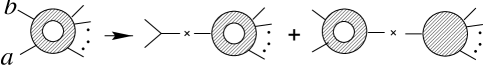
More explicitly, as two adjacent momenta $k_{1}$ and $k_{2}$ become collinear, we may factorize an $n$-point tree amplitude on the $s_{12}$ kinematic pole in terms of a three vertex and an $(n-1)$-point amplitude,

$\displaystyle{A_{n}^{{\rm tree}}(1,2,\ldots,n)}$ $\displaystyle{{}{\buildrel 1\parallel 2\over{\longrightarrow}}{\cal D}^{\mu,\,{\rm tree}}_{K\to 1,2}\left(i\sum_{\lambda}{\varepsilon^{-\lambda}_{\mu}(K)\varepsilon^{\lambda}_{\nu}(K)\over s_{12}}\right){\partial\over\partial\varepsilon^{\lambda}_{\nu}(K)}A^{{\rm tree}}_{n-1}(K^{\lambda},3,\dots)\,,}$
(3.1)

where $\lambda$ specifies the polarization and $k_{1}=zK$ and $k_{2}=(1-z)K$ with $K=k_{1}+k_{2}$. This basic structure is independent of the particle type, although we have written eq. (3.1) for the case of an intermediate gluon. The values of the ${\cal D^{\rm tree}}$ functions do however depend on the particle types and are simply given by the three-vertices

$\displaystyle{{\cal D}^{\mu,\,{\rm tree}}_{g\to g_{1}g_{2}}}$ $\displaystyle{{}=i\sqrt{2}(k_{1}^{\mu}\varepsilon_{1}\cdot\varepsilon_{2}+k_{2}\cdot\varepsilon_{1}\varepsilon_{2}^{\mu}-k_{1}\cdot\varepsilon_{2}\varepsilon_{1}^{\mu})\,,}$
$\displaystyle{{\cal D}^{\mu,\,{\rm tree}}_{g\to{\bar{q}}_{1}q_{2}}}$ $\displaystyle{{}={i\over\sqrt{2}}\overline{u}_{2}\gamma^{\mu}v_{1}\,,}$
$\displaystyle{{\cal D}^{j,\,{\rm tree}}_{q\to q_{1}g_{2}}}$ $\displaystyle{{}={i\over\sqrt{2}}\overline{u}_{j1}\raise 0.6458pt\hbox{/}\kern-5.00002pt\kern 0.16841pt\hbox{$\varepsilon$}\kern 0.16841pt_{2}\,.}$
(3.2)

In the first two cases $\mu$ represents the Lorentz index of the intermediate gluon which in the last case is replaced by a spinor index. Although it makes no difference in the results, we use the non-linear Gervais-Neveu [43] gauge since the vertices are particularly simple.

Refer to caption

Figure 2: The three vertices describing (a) ${\cal D}^{\mu,\,{\rm tree}}_{g\to g_{1}g_{2}}$, (b) ${\cal D}^{\mu,\,{\rm tree}}_{g\to{\bar{q}}_{1}q_{2}}$ and (c) ${\cal D}^{j,\,{\rm tree}}_{q\to q_{1}g_{2}}$.

After inserting an explicit representation of the helicity states [44], the collinear limits of tree amplitudes may be re-expressed as (see e.g. ref. [1])

$$A_{n}^{{\rm tree}}(1^{\lambda_{1}},2^{\lambda_{2}},\dots,n)\mathop{\longrightarrow}^{1\parallel 2}\ \sum_{\lambda=\pm}\mathop{\rm Split}\nolimits^{{\rm tree}}_{-\lambda}(1^{\lambda_{1}},2^{\lambda_{2}})\,A_{n-1}^{{\rm tree}}(K^{\lambda},3,\ldots,n)\,.$$ (3.3)

The splitting amplitudes in eq. (3.3) have square-root singularities in the collinear limit. For convenience we have collected the tree-level helicity splitting amplitudes in appendix A. For most computational purposes, the helicity form in eq. (3.3) is the more convenient one, but if one is working entirely in the context of conventional dimensional regularization where the polarization vectors become $(4-2\epsilon)$-dimensional, the representation in terms of formal polarization vectors and spinors is also useful.

The behavior of one-loop primitive amplitudes as the momenta of two adjacent legs becomes collinear is similar and is given by

$\displaystyle{A_{n}^{{1\mbox{-}\rm loop}}(1,2,\dots,n)}$ $\displaystyle{{}\mathop{\longrightarrow}^{1\parallel 2}\ {\cal D}^{\mu,\,{\rm tree}}_{K\to 1,2}\left(i\sum_{\lambda}{\varepsilon^{-\lambda}_{\mu}(K)\varepsilon^{\lambda}_{\nu}(K)\over s_{12}}\right){\partial\over\partial\varepsilon^{\lambda}_{\nu}(K)}A^{{1\mbox{-}\rm loop}}_{n-1}(K^{\lambda},3,\dots)}$
$\displaystyle{{}\hskip 28.45274pt+{\cal D}^{\mu,\,{1\mbox{-}\rm loop}}_{K\to 1,2}\left(i\sum_{\lambda}{\varepsilon^{-\lambda}_{\mu}(K)\varepsilon^{\lambda}_{\nu}(K)\over s_{12}}\right){\partial\over\partial\varepsilon^{\lambda}_{\nu}(K)}A^{{\rm tree}}_{n-1}(K^{\lambda},3,\dots)\,.}$
(3.4)

In the spinor helicity language, this becomes [26, 24]

$\displaystyle{A_{n}^{{1\mbox{-}\rm loop}}(1^{\lambda_{1}},2^{\lambda_{2}},\dots,n)}$ $\displaystyle{{}\mathop{\longrightarrow}^{1\parallel 2}\ \sum_{\lambda=\pm}\biggl{\{}\mathop{\rm Split}\nolimits^{{\rm tree}}_{-\lambda}(1^{\lambda_{1}},2^{\lambda_{2}})\,A_{n-1}^{{1\mbox{-}\rm loop}}(K^{\lambda},3,\ldots)}$
$\displaystyle{{}\hskip 56.9055pt+\mathop{\rm Split}\nolimits^{{1\mbox{-}\rm loop}}_{-\lambda}(1^{\lambda_{1}},2^{\lambda_{2}})\,A_{n-1}^{{\rm tree}}(K^{\lambda},3,\ldots)\biggr{\}}\,,}$
(3.5)

where $\lambda$ represents the helicity, $A_{n-1}^{{1\mbox{-}\rm loop}}$ and $A_{n}^{{\rm tree}}$ are one-loop and tree sub-amplitudes with a fixed ordering of legs with legs $1$ and $2$ consecutive in the ordering.

In section 4 we give expressions for the one-loop splitting functions ${\cal D}^{\mu,\,{1\mbox{-}\rm loop}}$ and $\mathop{\rm Split}\nolimits^{{1\mbox{-}\rm loop}}$ to all orders in the dimensional regularization parameter.

3.2 Soft behavior

In the limit that a gluon momentum becomes soft we may again factorize tree amplitudes on kinematic poles (see e.g. ref. [1]). In taking $k_{1}\to 0$ the two kinematic poles in the color ordered tree amplitude which may diverge are $1/s_{12}$ and $1/s_{n1}$ since $n$, $1$ and $2$ are consecutive legs in the cyclic color ordering. This yields the factorization relation

$$A_{n}^{\rm tree}(1^{\pm},2,\ldots,n)\mathop{\longrightarrow}^{k_{1}\to 0}\mathop{\cal S}\nolimits^{{\rm tree}}(n,1^{\pm},2)\,A_{n-1}^{\rm tree}(2,3,\ldots,n)\,.$$ (3.6)

In terms of polarization vectors, the tree-level soft function, $\mathop{\cal S}\nolimits^{{\rm tree}}$, is the familiar eikonal factor,

$$\mathop{\cal S}\nolimits^{{\rm tree}}(n,1^{\pm},2)=-{1\over\sqrt{2}}\left[{2\varepsilon^{\pm}_{1}\cdot k_{n}\over s_{n1}}-{2\varepsilon^{\pm}_{1}\cdot k_{2}\over s_{12}}\right]\,.$$ (3.7)

In spinor helicity notation, the soft amplitudes are,

$$\mathop{\cal S}\nolimits^{\rm tree}(n,1^{+},2)={\left\langle n\,2\right\rangle\over\left\langle n\,1\right\rangle\left\langle 1\,2\right\rangle}\,,\hskip 56.9055pt\mathop{\cal S}\nolimits^{\rm tree}(n,1^{-},2)={-\left[n\,2\right]\over\left[n\,1\right]\left[1\,2\right]}\,.$$ (3.8)

The soft amplitudes are independent of the helicities and particle types of the neighboring legs $n$ and $2$.

The behavior of one-loop gluon amplitudes in the soft limit is similar to the collinear behavior. As the momentum $k_{1}$ becomes soft the primitive one-loop amplitudes become

$$A_{n}^{1\mbox{-}\rm loop}(1,2,\ldots,n){{\buildrel k_{1}\to 0\over{\longrightarrow}}}\mathop{\cal S}\nolimits^{{\rm tree}}(n,1^{\pm},2)\,A_{n-1}^{1\mbox{-}\rm loop}(2,3,\ldots,n)+\mathop{\cal S}\nolimits^{1\mbox{-}\rm loop}(n,1^{\pm},2)\,A_{n-1}^{\rm tree}(2,3,\ldots,n)\,.$$ (3.9)

The one-loop soft function may be extracted from four- [40, 41, 45] and five-parton [22, 23, 24] one-loop amplitudes that are known through ${\cal O}(\epsilon^{0})$, with the result,

$$\mathop{\cal S}\nolimits^{{1\mbox{-}\rm loop}}(n,1^{\pm},2)=-\mathop{\cal S}\nolimits^{\rm tree}(n,1^{\pm},2)\,c_{\Gamma}\,\Bigl{[}{1\over\epsilon^{2}}\,\left({\mu^{2}(-s_{n2})\over(-s_{n1})(-s_{12})}\right)^{\epsilon}\,+{\pi^{2}\over 6}\Bigr{]}\,.$$ (3.10)

As for the collinear case, in section 4, we will generalize this to all orders in the dimensional regularization parameter. We will also generalize the discussion to include the case of one-loop primitive amplitudes with external fermions and present a representation in terms of formal polarization vectors. As we shall see, although the soft function does not depend on the neighboring external particles in the primitive ordering of legs, it does depend on whether the soft gluon is attached to a gluonic or fermionic part of the loop.

4 One-loop soft and collinear splitting amplitudes

In this section, we will apply the analysis of collinear limits and their relationship to infrared divergences of ref. [33] to obtain explicit expressions for the splitting amplitudes to all orders in the dimensional regulator, $\epsilon$. We shall also present explicit expressions for the soft amplitudes to all orders in $\epsilon$.

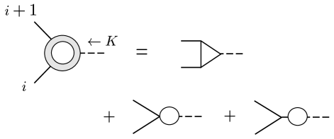
In our organization of the results, there are two contributions to the one-loop splitting amplitudes; the ‘factorizing’ and the ‘non-factorizing’ pieces, $\mathop{\rm Split}\nolimits^{{1\mbox{-}\rm loop}}=\mathop{\rm Split}\nolimits^{{\rm fact}}+\mathop{\rm Split}\nolimits^{{\rm non\hbox{-}fact}}$. The factorizing contributions are those which one naïvely expects for one-loop splitting. That is, they are derived from those diagrams, shown in fig. 3, in which one particle from a tree-level amplitude splits into two via a loop. They are called factorizing contributions because they factorize on a single particle propagator; one can amputate the splitting term from the diagram by cutting a single line.

Refer to caption

Figure 3: The diagrams in a massless theory (ignoring tadpoles) that need to be calculated to obtain the factorizing contribution to the loop splitting function. The dotted line represents the off-shell leg on which the collinear factorization is performed.

The non-factorizing contributions are quite different in nature. These arise from non-smooth behavior of infrared divergent integrals as a kinematic invariant vanishes. This non-smooth behavior arises because we take $\epsilon\rightarrow 0$ before we take the kinematic invariant to vanish. These non-factorizing contributions are proportional to the tree-level ones since the infrared singular parts of one-loop amplitudes are proportional to the tree-level amplitudes.

Although the division of the splitting amplitudes into factorizing and non-factorizing pieces contains some arbitrariness and is gauge dependent, the sum of the contributions is gauge independent. The calculation of the diagrams in fig. 3 always gives the complete non-singular contribution to the one-loop splitting amplitudes, but, depending on the gauge choice, also gives some portion of the infrared singular contribution. However, since the divergence structure of one-loop splitting amplitudes is known (see appendix B for their values through ${\cal O}(\epsilon^{0})$) and since each $1/\epsilon$ pole is uniquely identified with a known ‘discontinuity function’ (see reference [33] and section 4.2 below) we can push all singularities into the non-factorizing piece, and define the factorizing piece to be the infrared finite part of the diagrams in fig. 3, not involving any of the discontinuity functions. The non-factorizing contribution may then be determined by finding the linear combination of discontinuity functions that matches the known infrared divergence structure of the amplitudes.

We will first compute the diagrams that yield the factorizing parts of the one-loop splitting amplitudes. We then use the known structure of the infrared singularities of the leading partial amplitudes to derive the non-factorizing contributions to one-loop splitting. By combining the factorizing and non-factorizing parts we obtain the full one-loop splitting amplitudes for the leading partial amplitudes. Finally, we will derive the soft factorization properties of one-loop amplitudes. Our results will be in terms of the bare splitting amplitudes; in section 4.4 we give the appropriate ultraviolet subtraction for obtaining the splitting amplitudes for the renormalized amplitudes.

4.1 Factorizing contributions to the one-loop splitting amplitudes

The factorizing contributions to one-loop splitting amplitudes are determined by computing triangle and bubble diagrams like those shown in fig. 3. Any poles in $\epsilon$ that appear must come from one of two discontinuity functions [33],

$\displaystyle{f_{1}(s_{12},\epsilon)}$ $\displaystyle{{}={1\over\epsilon(1-2\epsilon)}\left({\mu^{2}\over-s_{12}}\right)^{\epsilon}\,,}$
$\displaystyle{f_{2}(s_{12},\epsilon)}$ $\displaystyle{{}=-{1\over\epsilon^{2}}\left({\mu^{2}\over-s_{12}}\right)^{\epsilon}\,.}$
(4.1)

After removing the poles by subtracting off terms proportional to these discontinuity functions the factorizing contribution to the splitting function is determined by inserting a complete set of states on the (off-shell) fused leg, imposing the collinear limit and then taking the fused leg on-shell.

The results below are computed in the Feynman background field gauge and apply to an $SU(N_{c})$ gauge theory with matter content of $n_{f}$ flavors of massless Dirac fermions in the fundamental representation and $n_{s}$ flavors of massless complex scalars in the $(N_{c}+\overline{N}_{c})$ representation. In each case, we describe a parton splitting into two final state partons labeled $1$ and $2$ which carry momentum fractions $z$ and $1-z$ respectively.

The difference between dimensional regularization schemes is parameterized by the quantity $\delta_{R}$. In the dimensional reduction [46] or four-dimensional helicity [41] schemes used to compute one-loop helicity amplitudes, both external gluons and those inside loops, have two polarization states. In these schemes, $\delta_{R}=0$. In the ’t Hooft–Veltman scheme, external gluons have two polarization states, but those inside loops have $[\epsilon]$-helicities, i.e. polarization states that point into the extra $-2\epsilon$ dimensions. For this scheme, $\delta_{R}=1$. In conventional dimensional regularization all gluons, external and internal, have $[\epsilon]$-helicities. The $[\epsilon]$-helicities of the internal gluons are accounted for by setting $\delta_{R}=1$; those of the external gluons must be accounted for by spin sums over $D$-dimensional polarization vectors.

4.1.1 Factorizing contributions to one-loop $g\to gg$ splitting amplitudes

The result of the triangle and bubble graphs is (after stripping the coupling and color factors) [33]

$${\cal D}_{g\to g_{1}g_{2}}^{\mu,\,{\rm fact}}={i\over\sqrt{2}}{\tau_{\Gamma}\over 3}\left(1-\epsilon\delta_{R}-{n_{f}\over N_{c}}+{n_{s}\over N_{c}}\right)(k_{1}-k_{2})^{\mu}\left[{\left({\varepsilon_{1}}\!\cdot\!{\varepsilon_{2}}\right)}-{{\left({k_{1}}\!\cdot\!{\varepsilon_{2}}\right)}{\left({k_{2}}\!\cdot\!{\varepsilon_{1}}\right)}\over{\left({k_{1}}\!\cdot\!{k_{2}}\right)}}\right]\,,$$ (4.2)

where

$$\tau_{\Gamma}^{\vphantom{A}}\equiv\left({\mu^{2}\over-s_{12}}\right)^{\epsilon}c_{\Gamma}{6\over(1-2\epsilon)(2-2\epsilon)(3-2\epsilon)}\,,$$ (4.3)

and

$$c_{\Gamma}={1\over\left(4\pi\right)^{2-\epsilon}}{\Gamma(1+\epsilon)\Gamma^{2}(1-\epsilon)\over\Gamma(1-2\epsilon)}\,.$$ (4.4)

In background field Feynman gauge, which is a convenient gauge for evaluating the diagrams, ${\cal D}_{g\to g_{1}g_{2}}^{\mu,\,{\rm fact}}$ is finite due to a Ward identity, so no discontinuity functions need to be subtracted off. The factorizing part of the one loop splitting function, ${\mathop{\rm Split}\nolimits}^{{\rm fact}}_{-\lambda}(1^{\lambda_{1}},2^{\lambda_{2}})$ (where the $\lambda$’s label helicities and are defined as if all particles exit the diagram), is derived from ${\cal D}$ by

$\displaystyle{A_{n}^{{\rm fact}}}$ $\displaystyle{{}{\buildrel 1\parallel 2\over{\longrightarrow}}{\cal D}^{\mu,\,{\rm fact}}_{g\to g_{1}g_{2}}({\lambda_{1}},{\lambda_{2}})\left(i\sum_{\lambda=\pm}{\varepsilon^{-\lambda}_{\mu}(K)\varepsilon^{\lambda}_{\nu}(K)\over 2k_{1}\cdot k_{2}}\right){\partial\over\partial\varepsilon^{\lambda}_{\nu}(K)}A^{{\rm tree}}_{n-1}(\dots K^{\lambda}\dots)}$
$\displaystyle{{}=\sum_{\lambda=\pm}{\mathop{\rm Split}\nolimits}^{{\rm fact}}_{-\lambda}(1^{\lambda_{1}},2^{\lambda_{2}})A^{{\rm tree}}_{n-1}(\dots K^{\lambda}\dots).}$
(4.5)

This yields

$\displaystyle{{\mathop{\rm Split}\nolimits}^{{\rm fact}}_{-\lambda}(1^{\lambda_{1}},2^{\lambda_{2}})}$ $\displaystyle{{}=-{\tau_{\Gamma}\over 3}\left(1-\epsilon\delta_{R}-{n_{f}\over N_{c}}+{n_{s}\over N_{c}}\right){\varepsilon^{-\lambda}(K)\!\cdot\!\left(k_{1}-k_{2}\right)\over 2\sqrt{2}{\left({k_{1}}\!\cdot\!{k_{2}}\right)}}\left[{\left({\varepsilon_{1}}\!\cdot\!{\varepsilon_{2}}\right)}-{{\left({k_{1}}\!\cdot\!{\varepsilon_{2}}\right)}{\left({k_{2}}\!\cdot\!{\varepsilon_{1}}\right)}\over{\left({k_{1}}\!\cdot\!{k_{2}}\right)}}\right]\,,}$
(4.6)

where $K=k_{1}+k_{2}$. Expressed in terms of spinor inner products [44, 1] the result is that

$\displaystyle{{\mathop{\rm Split}\nolimits}^{{\rm fact}}_{+}(1^{+},2^{+})=\ }$ $\displaystyle{{}-{\tau_{\Gamma}\over 3}\left(1-\epsilon\delta_{R}-{n_{f}\over N_{c}}+{n_{s}\over N_{c}}\right)\sqrt{z(1-z)}{\left[1\,2\right]\over{\left\langle 1\,2\right\rangle}^{2}}}$
$\displaystyle{{\mathop{\rm Split}\nolimits}^{{\rm fact}}_{+}(1^{-},2^{-})=\ }$ $\displaystyle{{}-{\tau_{\Gamma}\over 3}\left(1-\epsilon\delta_{R}-{n_{f}\over N_{c}}+{n_{s}\over N_{c}}\right)\sqrt{z(1-z)}{1\over\left[1\,2\right]},}$
$\displaystyle{{\mathop{\rm Split}\nolimits}^{{\rm fact}}_{+}(1^{+},2^{-})=\ }$ $\displaystyle{{}{\mathop{\rm Split}\nolimits}^{{\rm fact}}_{+}(1^{-},2^{+})=\ 0\,,}$
(4.7)

with the remaining terms, ${\mathop{\rm Split}\nolimits}_{-}(1^{\lambda_{1}},2^{\lambda_{2}})$, given by parity inversion. Except for ${\mathop{\rm Split}\nolimits}_{+}(1^{+},2^{+})$ and ${\mathop{\rm Split}\nolimits}_{-}(1^{-},2^{-})$ which vanish at tree level, the factorizing contributions to the one loop splitting amplitudes are proportional to the tree-level splitting amplitudes,

$${\mathop{\rm Split}\nolimits}^{{\rm fact}}_{-\lambda}(1^{\lambda_{1}},2^{\lambda_{2}})=c_{\Gamma}{\mathop{\rm Split}\nolimits}^{{\rm tree}}_{-\lambda}(1^{\lambda_{1}},2^{\lambda_{2}})r^{g\to g_{1}g_{2},\,{{\rm fact}}}_{S}(-\lambda,1^{\lambda_{1}},2^{\lambda_{2}})\,,$$ (4.8)

where

$\displaystyle{r^{g\to g_{1}g_{2},\,{{\rm fact}}}_{S}(\lambda,1^{\pm},2^{\mp})}$ $\displaystyle{{}=0\,,}$
$\displaystyle{r^{g\to g_{1}g_{2},\,{{\rm fact}}}_{S}(\pm,1^{\mp},2^{\mp})}$ $\displaystyle{{}=\left({\mu^{2}\over-s_{12}}\right)^{\epsilon}\left(1-\epsilon\delta_{R}-{n_{f}\over N_{c}}+{n_{s}\over N_{c}}\right){2z(1-z)\over(1-2\epsilon)(2-2\epsilon)(3-2\epsilon)}\,.}$
(4.9)

4.1.2 Factorizing contributions to one-loop $g\to\overline{q}q$ splitting amplitudes

For $g\to\overline{q}q$ splitting, the sum of the color and coupling stripped triangle and bubble graphs is

$\displaystyle{\widetilde{\cal D}^{\mu,\,{\rm fact}}_{g\to\overline{q}_{1}q_{2}}}$ $\displaystyle{{}=i{c_{\Gamma}\over\sqrt{2}}\left({\mu^{2}\over-s_{12}}\right)^{\epsilon}\overline{u}_{2}\gamma^{\mu}v_{1}\left\{\vphantom{\left[{(\delta_{R})\over(3)}\right.}\right.}$
$\displaystyle{{}\left[{13\over 6\epsilon(1-2\epsilon)}+{1\over 3(1-2\epsilon)(3-2\epsilon)}+{(1-\delta_{R})\over(1-2\epsilon)(2-2\epsilon)(3-2\epsilon)}\right]}$
$\displaystyle{{}-{1\over N_{c}^{2}}\left[-{1\over\epsilon^{2}}-{3\over 2\epsilon(1-2\epsilon)}-{1\over 1-2\epsilon}+{1-\delta_{R}\over(2-2\epsilon)}\right]}$
$\displaystyle{{}\left.\hbox{}+{1\over N_{c}}\left[-{2n_{f}+n_{s}\over 3\epsilon(1-2\epsilon)}+{2(n_{f}-n_{s})\over 3(1-2\epsilon)(3-2\epsilon)}\right]\vphantom{\left[{(\delta_{R})\over(3)}\right.}\right\}\,.}$
(4.10)

Here we see a number of terms that are proportional to the discontinuity functions $f_{1}$ and $f_{2}$. After removing these terms, we have,

$\displaystyle{{\cal D}^{\mu,\,{\rm fact}}_{g\to\overline{q}_{1}q_{2}}}$ $\displaystyle{{}=i{c_{\Gamma}\over\sqrt{2}}\left({\mu^{2}\over-s_{12}}\right)^{\epsilon}\overline{u}_{2}\gamma^{\mu}v_{1}\left\{{5-2\epsilon-3\delta_{R}\over 3(1-2\epsilon)(2-2\epsilon)(3-2\epsilon)}\right.}$
$\displaystyle{{}\left.\hbox{}+{1\over N_{c}^{2}}{1+\delta_{R}(1-2\epsilon)\over(1-2\epsilon)(2-2\epsilon)}+{n_{f}-n_{s}\over N_{c}}{2\over 3(1-2\epsilon)(3-2\epsilon)}\right\}\,.}$
(4.11)

After inserting a complete set of helicity states in an expression analogous to eq. (4.6), we find that the one loop splitting function is proportional to the tree-level result for each allowed helicity configuration. With $r^{g\to\overline{q}_{1}q_{2},\,{{\rm fact}}}_{S}$ defined as in eq. (4.8), we have,

$\displaystyle{r^{g\to\overline{q}_{1}q_{2},\,{{\rm fact}}}_{S}(\lambda,1^{\pm},2^{\mp})}$ $\displaystyle{{}=\left({\mu^{2}\over-s_{12}}\right)^{\epsilon}\left[{5-2\epsilon-3\delta_{R}\over 3(1-2\epsilon)(2-2\epsilon)(3-2\epsilon)}+{1\over N_{c}^{2}}{1+\delta_{R}(1-2\epsilon)\over(1-2\epsilon)(2-2\epsilon)}\right.}$
$\displaystyle{{}\phantom{\left({\mu^{2}\over-s_{12}}\right)^{\epsilon}\qquad}\left.\hbox{}+{n_{f}-n_{s}\over N_{c}}{2\over 3(1-2\epsilon)(3-2\epsilon)}\right]\,.}$
(4.12)

4.1.3 Factorizing contributions to one-loop $q\to qg$ splitting amplitudes

For $q\to qg$ splitting, the sum of the coupling and color stripped triangle and bubble graphs is

$\displaystyle{\widetilde{\cal D}^{i,\,{\rm fact}}_{q\to q_{1}g_{2}}}$ $\displaystyle{{}=-i{c_{\Gamma}\over\sqrt{2}}\left({\mu^{2}\over-s_{12}}\right)^{\epsilon}\left[\overline{u}_{i1}\raise 0.6458pt\hbox{/}\kern-5.00002pt\kern 0.16841pt\hbox{$\varepsilon$}\kern 0.16841pt_{2}-{\overline{u}_{i1}\kern 0.2604pt\raise 0.6458pt\hbox{/}\kern 0.2604pt\kern-5.52084pt\hbox{$k$}_{2}{\left({k_{1}}\!\cdot\!{\varepsilon_{2}}\right)}\over{\left({k_{1}}\!\cdot\!{k_{2}}\right)}}\right]\times}$
$\displaystyle{{}\hskip 36.135pt\left[{1\over\epsilon^{2}}+{N_{c}^{2}-1\over N_{c}^{2}}{1\over\epsilon(1-2\epsilon)}-{N_{c}^{2}+1\over N_{c}^{2}}{1-\epsilon\delta_{R}\over(1-2\epsilon)(2-2\epsilon)}\right]\,.}$
(4.13)

After subtracting out terms proportional to the discontinuity functions, we get

$${\cal D}^{i,\,{\rm fact}}_{q\to q_{1}g_{2}}=i{c_{\Gamma}\over\sqrt{2}}\left({\mu^{2}\over-s_{12}}\right)^{\epsilon}\left[\overline{u}_{i1}\raise 0.6458pt\hbox{/}\kern-5.00002pt\kern 0.16841pt\hbox{$\varepsilon$}\kern 0.16841pt_{2}-{\overline{u}_{i1}\kern 0.2604pt\raise 0.6458pt\hbox{/}\kern 0.2604pt\kern-5.52084pt\hbox{$k$}_{2}{\left({k_{1}}\!\cdot\!{\varepsilon_{2}}\right)}\over{\left({k_{1}}\!\cdot\!{k_{2}}\right)}}\right]{N_{c}^{2}+1\over N_{c}^{2}}{1-\epsilon\delta_{R}\over(1-2\epsilon)(2-2\epsilon)}\,.$$ (4.14)

Following the same procedure as above, we find that

$\displaystyle{r^{q\to q_{1}g_{2},\,{{\rm fact}}}_{S}(\pm,1^{\mp},2^{\pm})}$ $\displaystyle{{}=0\,,}$
$\displaystyle{r^{q\to q_{1}g_{2},\,{{\rm fact}}}_{S}(\pm,1^{\mp},2^{\mp})}$ $\displaystyle{{}=\left({\mu^{2}\over-s_{12}}\right)^{\epsilon}\left(1+{1\over N_{c}^{2}}\right){(1-z)(1-\epsilon\delta_{R})\over(1-2\epsilon)(2-2\epsilon)}\,.}$
(4.15)

For ${\bar{q}}\to g_{1}{\bar{q}}_{2}$ splitting, we need simply interchange $z$ and $1-z$.

4.2 Non-factorizing contributions

In ref. [33] it was shown that all non-factorizing contributions may be linked to infrared divergences which have a universal structure for an arbitrary number of external legs. The coefficients of the infrared divergences may be used to fix the coefficients of all integral functions associated with non-factorizing contributions to the splitting amplitudes.

The integral functions to be used are selected by demanding that they contain no infrared divergences other than ones which may appear in the splitting amplitudes. The infrared divergences of the integral functions may be obtained from the explicit forms of the integrals contained in, for example, refs. [33, 47]. By systematically stepping through the list of all integrals and their discontinuities one can construct a list of infrared divergent functions (and their associated higher order in $\epsilon$ parts) that may appear in the soft or collinear splitting amplitudes.

More explicitly, the complete one-loop splitting amplitudes are given by

$$\mathop{\rm Split}\nolimits^{{1\mbox{-}\rm loop}}(1,2)=\mathop{\rm Split}\nolimits^{{\rm fact}}(1,2)+c_{1}f_{1}(s_{12},\epsilon)+c_{2}f_{2}(s_{12},\epsilon)+c_{3}f_{3}(s_{12},\epsilon,z)+c_{4}f_{4}(s_{12},\epsilon,z)\,,$$ (4.16)

where the $c_{i}$ are coefficients to be fixed using known infrared divergences and the discontinuity functions are (see appendix C)

$\displaystyle{f_{1}(s_{12},\epsilon)}$ $\displaystyle{{}=-i\mu^{2\epsilon}{\cal I}_{2}(s_{12})={c_{\Gamma}\over\epsilon(1-2\epsilon)}\Bigl{(}{\mu^{2}\over-s_{12}}\Bigr{)}^{\epsilon}\,,}$
$\displaystyle{f_{2}(s_{12},\epsilon)}$ $\displaystyle{{}=-i\mu^{2\epsilon}{\cal I}_{3}(s_{12})=-{c_{\Gamma}\over\epsilon^{2}}\Bigl{(}{\mu^{2}\over-s_{12}}\Bigr{)}^{\epsilon}\,,}$
$\displaystyle{f_{3}(s_{12},\epsilon,z)}$ $\displaystyle{{}=-f_{2}(s_{12},\epsilon)+\lim_{k_{1}\parallel k_{2}}{i\over 2}\mu^{2\epsilon}s_{n1}s_{12}\,{\cal I}^{\rm 1m}_{4:3}={c_{\Gamma}\over\epsilon^{2}}\left({\mu^{2}\over-s_{12}}\right)^{\epsilon}\sum_{m=1}^{\infty}\epsilon^{m}{\mathop{\hbox{\rm Li}}\nolimits}_{m}\left({1-z\over-z}\right)\,,}$
$\displaystyle{f_{4}(s_{12},\epsilon,z)}$ $\displaystyle{{}=-f_{2}(s_{12},\epsilon)+\lim_{k_{1}\parallel k_{2}}{i\over 2}\mu^{2\epsilon}s_{12}s_{23}\,{\cal I}^{\rm 1m}_{4:4}={c_{\Gamma}\over\epsilon^{2}}\left({\mu^{2}\over-s_{12}}\right)^{\epsilon}\sum_{m=1}^{\infty}\epsilon^{m}{\mathop{\hbox{\rm Li}}\nolimits}_{m}\left({-z\over 1-z}\right)\,,}$
(4.17)

where ${\mathop{\hbox{\rm Li}}\nolimits}_{m}(x)$ is the $m{\rm th}$ polylogarithm [48]

$$\left.\begin{array}[]{l}{\mathop{\hbox{\rm Li}}\nolimits}_{1}(x)\ =-\ln(1-x)\\ \displaystyle{\mathop{\hbox{\rm Li}}\nolimits}_{m}(x)=\int_{0}^{x}{dt\over t}\,{\mathop{\hbox{\rm Li}}\nolimits}_{m-1}(t)\qquad(m=2,3,\dots)\end{array}\right\}=\sum_{n=1}^{\infty}{x^{n}\over n^{m}},$$

The scalar integrals appearing in the discontinuity functions are

$\displaystyle{{\rm(a)}\hskip 14.22636pt}$ $\displaystyle{{}{\cal I}_{2}(s_{12})=\int{d^{4-2\epsilon}p\over(2\pi)^{4-2\epsilon}}\,{1\over p^{2}(p-k_{1}-k_{2})^{2}}\,,}$
$\displaystyle{{\rm(b)}\hskip 14.22636pt}$ $\displaystyle{{}{\cal I}_{3}(s_{12})=\int{d^{4-2\epsilon}p\over(2\pi)^{4-2\epsilon}}\,{1\over p^{2}(p-k_{1})^{2}(p-k_{1}-k_{2})^{2}}\,,}$
$\displaystyle{{\rm(c)}\hskip 14.22636pt}$ $\displaystyle{{}{\cal I}^{\rm 1m}_{4:3}(s_{n1},s_{12})=\int{d^{4-2\epsilon}p\over(2\pi)^{4-2\epsilon}}\,{1\over p^{2}(p-k_{1})^{2}(p-k_{1}-k_{2})^{2}(p+k_{n})^{2}}\,,}$
$\displaystyle{{\rm(d)}\hskip 14.22636pt}$ $\displaystyle{{}{\cal I}^{\rm 1m}_{4:4}(s_{12},s_{23})=\int{d^{4-2\epsilon}p\over(2\pi)^{4-2\epsilon}}\,{1\over p^{2}(p-k_{1})^{2}(p-k_{1}-k_{2})^{2}(p-k_{1}-k_{2}-k_{3})^{2}}\,.}$
(4.18)

These integrals are depicted in fig. 4. No other integrals appear because they are either smooth functions in the collinear limits, or they do not have the correct infrared divergences to match those appearing in the splitting amplitudes [33]. It is easy to see from eq. (4.17) that $f_{4}(s_{12},\epsilon,z)=f_{3}(s_{12},\epsilon,1-z)$. This relation is apparent even in the integral function by shifting the loop momentum of ${\cal I}^{\rm 1m}_{4:4}(s_{12},s_{23})$ such that $p\to-p+k_{1}+k_{2}$.

Refer to caption

Figure 4: The scalar integrals that can appear in the collinear splitting amplitudes. Legs 1 and 2 are collinear.

To fix the coefficients $c_{i}$ we proceed as follows. An $n$-point primitive amplitude will have a known singular structure of the form [18, 3, 19],

$$A_{n}^{{1\mbox{-}\rm loop}}\Bigr{|}_{\rm singular}=-c_{\Gamma}A_{n}^{{\rm tree}}\left[{1\over\epsilon^{2}}\sum_{j=1}^{n}s_{j}^{[n]}\left({\mu^{2}\over-s_{j,j+1}}\right)^{\epsilon}+{c^{[n]}\over\epsilon}\right]\,,$$ (4.19)

where the coefficients $s^{[n]}_{j}$ and $c^{[n]}$ depend on the particular $n$-point amplitude under consideration. Consider now the collinear or soft limits given in eqs. (3.5) and (3.9). The $n-1$ point amplitudes appearing on the right-hand-side of these equations can have a different set of singularities. The difference between these two sets of known singularities must then be absorbed into the splitting or soft amplitudes $\mathop{\rm Split}\nolimits^{1\mbox{-}\rm loop}$ or $\mathop{\cal S}\nolimits^{1\mbox{-}\rm loop}$. More directly, we can use the known results for the splitting amplitudes through ${\cal O}(\epsilon^{0})$, which we have collected in appendix B, to determine the singularities. Using table 1 we can then uniquely determine all $c_{i}$ coefficients appearing in eq. (4.16). The unique $1/\epsilon$ singularities of the functions are listed in the first column of the table. The second column lists the discontinuity function associated with each singularity. One adjusts the $c_{i}$ coefficients so that the divergences in the splitting amplitudes are correct. This uniquely fixes the splitting amplitudes to all orders in the dimensional regularization parameter $\epsilon$.

Singularity Non-Factorizing Contribution
$\displaystyle\vphantom{\Bigg{|}^{A}}{c_{\Gamma}\over\epsilon}$ $\displaystyle f_{1}(s_{12},\epsilon)$
$\displaystyle\vphantom{\Bigg{|}^{A}}{c_{\Gamma}\ln(-s_{i,i+1})\over\epsilon}$ $\displaystyle f_{2}(s_{12},\epsilon)$
$\displaystyle\vphantom{\Bigg{|}^{A}}{c_{\Gamma}\ln(z)\over\epsilon}$ $\displaystyle f_{3}(s_{12},\epsilon,z)$
$\displaystyle\vphantom{\Bigg{|}^{A}}{c_{\Gamma}\ln(1-z)\over\epsilon}$ $\displaystyle f_{3}(s_{12},\epsilon,1-z)$
Table 1: The potential ‘non-factorizing’ contributions to the splitting amplitudes in the $k_{1}\parallel k_{2}$ channel.

Since the divergences of the primitive amplitudes are always proportional to tree amplitudes, the non-factorizing contributions to one-loop splitting amplitudes will all be proportional to the tree-level splitting amplitudes. In analogy to eq. (4.8), we write

$${\mathop{\rm Split}\nolimits}^{{\rm non\hbox{-}fact}}_{-\lambda}(1^{\lambda_{1}},2^{\lambda_{2}})=c_{\Gamma}\,{\mathop{\rm Split}\nolimits}^{{\rm tree}}_{-\lambda}(1^{\lambda_{1}},2^{\lambda_{2}})\,r^{{\rm non\hbox{-}fact}}_{S}\,,$$ (4.20)

for each type of splitting function. There is no need to specify the helicity structure of $r^{{\rm non\hbox{-}fact}}_{S}$ because the factor is the same for all allowed helicity configurations. For the ${\cal D}$ functions we can write

$${\cal D}^{\mu,\,{\rm non\hbox{-}fact}}_{K\to 1,2}=c_{\Gamma}\,{\cal D}^{\mu,\,{\rm tree}}_{K\to 1,2}\,r^{{\rm non\hbox{-}fact}}_{S}\,.$$ (4.21)

4.2.1 Non-factorizing contributions to one loop $g\to gg$ splitting amplitudes

In order to demonstrate the procedure more explicitly, we extract the non-factorizing contributions to one-loop $g\to gg$ splitting using pure gluon amplitudes. The unrenormalized pole structure of the leading $n$ gluon partial amplitude $A_{n:1}(1,2,\dots,n)$ is

$$A^{ng}_{n:1}\Big{|}_{\rm singular}=\ -c_{\Gamma}A_{n}^{ng,\,{\rm tree}}\left[{1\over\epsilon^{2}}\sum_{j=1}^{n}\left({\mu^{2}\over-s_{j,j+1}}\right)^{\epsilon}+{2\over\epsilon}\left({11\over 6}-{1\over 3}{n_{f}\over N_{c}}-{1\over 6}{n_{s}\over N_{c}}\right)\right]\,,$$ (4.22)

where we identify the label $n+1$ with $1$. In the limit that gluons $1$ and $2$ become collinear, we verify that for the helicity configurations forbidden at tree-level,

$$\mathop{\rm Split}\nolimits^{g\to g_{1}g_{2},\,{{\rm non\hbox{-}fact}}}(\pm,1^{\pm},2^{\pm})=0\,,$$ (4.23)

while for all configurations allowed at tree-level

$$r^{g\to g_{1}g_{2},\,{{\rm non\hbox{-}fact}}}_{S}=-{1\over\epsilon^{2}}+{\ln(-s_{12})\over\epsilon}+{\ln(z)\over\epsilon}+{\ln(1-z)\over\epsilon}+{\cal O}(\epsilon^{0})\,.$$ (4.24)

This may also be read off from the known results [26, 24] for the splitting amplitudes through ${\cal O}(\epsilon^{0})$ which we have collected in appendix B. Focusing on the $1/\epsilon$ poles we use table 1 to deduce that

$$r^{g\to g_{1}g_{2},\,{{\rm non\hbox{-}fact}}}_{S}=\ f_{2}(s_{12},\epsilon)+f_{3}(s_{12},\epsilon,z)+f_{3}(s_{12},\epsilon,1-z)\,,$$ (4.25)

where the discontinuity functions $f_{i}$ are defined in eq. (4.17). The combination of functions appearing here may be further simplified using eq. (C.10).

4.2.2 Non-factorizing contributions to one-loop $g\to\overline{q}q$ splitting amplitudes

To extract the non-factorizing contributions to one-loop $g\to\overline{q}q$ splitting we need the unrenormalized pole structure of the leading all-gluon partial amplitudes, eq. (4.22), as well as that of the leading two quark partial amplitudes $A_{n:1}(1_{\overline{q}},2_{q},3,\dots,n)$,

$$A^{2q}_{n:1}\Big{|}_{\rm singular}=\ -c_{\Gamma}A_{n}^{2q,\,{\rm tree}}\left[{1\over\epsilon^{2}}\sum_{j=2}^{n}\left({\mu^{2}\over-s_{j,j+1}}\right)^{\epsilon}-{1\over N_{c}^{2}}{1\over\epsilon^{2}}\left({\mu^{2}\over-s_{12}}\right)^{\epsilon}+{3\over 2\epsilon}\left(1-{1\over N_{c}^{2}}\right)\right]\,.$$ (4.26)

From this it follows that

$\displaystyle{r^{g\to\overline{q}_{1}q_{2},\,{{\rm non\hbox{-}fact}}}_{S}=}$
$\displaystyle{{1\over\epsilon^{2}}{1\over N_{c}^{2}}+{1\over\epsilon}\left(\ln(z)+\vphantom{{\ln(-s_{12})\over N_{c}^{2}}}\right.}$ $\displaystyle{{}\left.\ln(1-z)-{\ln(-s_{12})\over N_{c}^{2}}+{13\over 6}+{3\over 2N_{c}^{2}}-{2n_{f}\over 3}-{n_{s}\over 3}\right)+{\cal O}(\epsilon^{0})\,.}$
(4.27)

As before, this may also be obtained from the known results for the splitting amplitudes through ${\cal O}(\epsilon^{0})$ which we have collected in appendix B. Again, focusing on the $1/\epsilon$ poles, we read off

$\displaystyle{r^{g\to\overline{q}_{1}q_{2},\,{{\rm non\hbox{-}fact}}}_{S}=\ f_{3}(s_{12},\epsilon,z)}$ $\displaystyle{{}+f_{3}(s_{12},\epsilon,1-z)-{1\over N_{c}^{2}}f_{2}(s_{12},\epsilon)}$ $\displaystyle{{}+\left[{13\over 6}+{3\over 2N_{c}^{2}}-{2n_{f}\over 3N_{c}}-{n_{s}\over 3N_{c}}\right]f_{1}(s_{12},\epsilon)\,.}$ (4.28)

4.2.3 Non-factorizing contributions to one loop $q\to qg$ splitting amplitudes

We need only the pole structure of the leading two quark partial amplitudes, eq. (4.26), to derive the non-factorizing contributions to one-loop $q\to qg$ splitting. From

$$r^{q\to q_{1}g_{2},\,{{\rm non\hbox{-}fact}}}_{S}=-{1\over\epsilon^{2}}+{1\over\epsilon}\left(\ln(-s_{12})+\ln(1-z)-{\ln(z)\over N_{c}^{2}}\right)+{\cal O}(\epsilon^{0})\,,$$ (4.29)

we obtain

$$r^{q\to q_{1}g_{2},\,{{\rm non\hbox{-}fact}}}_{S}=f_{2}(s_{12},\epsilon)+f_{3}(s_{12},\epsilon,1-z)-{1\over N_{c}^{2}}f_{3}(s_{12},\epsilon,z)\,.$$ (4.30)

Again, for ${\bar{q}}\to g_{1}{\bar{q}}_{2}$ splitting we simply interchange $z$ and $1-z$.

4.3 Full one-loop splitting amplitudes for leading color partial amplitudes to all orders in $\epsilon$.

We now combine the factorizing and non-factorizing terms to give the full one loop splitting amplitudes for leading partial amplitudes to all orders in $\epsilon$.

For $g\to g_{1}g_{2}$ splitting, there is one independent helicity configuration that is non-zero at one loop but vanishes at tree-level,

$\displaystyle{\mathop{\rm Split}\nolimits^{g\to gg,\,{{1\mbox{-}\rm loop}}}_{+}(1^{+},2^{+})=\ }$
$\displaystyle{-\sqrt{z(1-z)}{\left[1\,2\right]\over{\left\langle 1\,2\right\rangle}^{2}}}$ $\displaystyle{{}{2c_{\Gamma}\over(1-2\epsilon)(2-2\epsilon)(3-2\epsilon)}\left({\mu^{2}\over-s_{12}}\right)^{\epsilon}\left(1-\epsilon\delta_{R}-{n_{f}\over N_{c}}+{n_{s}\over N_{c}}\right)\,.}$
(4.31)

We present the rest of the splitting amplitudes in terms of $r_{S}$.

$\displaystyle{r^{g\to g_{1}g_{2},\,{{1\mbox{-}\rm loop}}}_{S}(\pm,1^{\mp},2^{\mp})=\ \left({\mu^{2}\over-s_{12}}\right)^{\epsilon}}$ $\displaystyle{{}\left\{{1\over\epsilon^{2}}\left[-\left({1-z\over z}\right)^{\epsilon}{\pi\epsilon\over\sin(\pi\epsilon)}+\sum_{m=1}^{\infty}2\epsilon^{2m-1}{\mathop{\hbox{\rm Li}}\nolimits}_{2m-1}\left({-z\over 1-z}\right)\right]\right.}$
$\displaystyle{{}\left.\hbox{}+{2z(1-z)\over(1-2\epsilon)(2-2\epsilon)(3-2\epsilon)}\left(1-\epsilon\delta_{R}-{n_{f}\over N_{c}}+{n_{s}\over N_{c}}\right)\vphantom{\left[\sum_{m=0}^{\infty}\right]}\right\}\,,}$
$\displaystyle{r^{g\to g_{1}g_{2},\,{{1\mbox{-}\rm loop}}}_{S}(\lambda,1^{\pm},2^{\mp})=\ \left({\mu^{2}\over-s_{12}}\right)^{\epsilon}}$ $\displaystyle{{}{1\over\epsilon^{2}}\left[-\left({1-z\over z}\right)^{\epsilon}{\pi\epsilon\over\sin(\pi\epsilon)}+\sum_{m=1}^{\infty}2\epsilon^{2m-1}{\mathop{\hbox{\rm Li}}\nolimits}_{2m-1}\left({-z\over 1-z}\right)\right]\,.}$
(4.32)

In terms of formal polarization vectors,

$\displaystyle{{\cal D}^{\mu,\,{1\mbox{-}\rm loop}}_{g\to g_{1}g_{2}}=\ }$ $\displaystyle{{}{i\sqrt{2}}(k_{1}-k_{2})^{\mu}\left[{\left({\varepsilon_{1}}\!\cdot\!{\varepsilon_{2}}\right)}-{{\left({k_{1}}\!\cdot\!{\varepsilon_{2}}\right)}{\left({k_{2}}\!\cdot\!{\varepsilon_{1}}\right)}\over{\left({k_{1}}\!\cdot\!{k_{2}}\right)}}\right]\left({\mu^{2}\over-s_{12}}\right)^{\epsilon}{c_{\Gamma}\left(1-\epsilon\delta_{R}-{n_{f}\over N_{c}}+{n_{s}\over N_{c}}\right)\over(1-2\epsilon)(2-2\epsilon)(3-2\epsilon)}}$
$\displaystyle{{}+i\sqrt{2}[k_{1}^{\mu}\varepsilon_{1}\cdot\varepsilon_{2}+k_{2}\cdot\varepsilon_{1}\varepsilon_{2}^{\mu}-(k_{1}+k_{2})\cdot\varepsilon_{2}\varepsilon_{1}^{\mu}]\times}$
$\displaystyle{{}\hskip 28.45274pt\left({\mu^{2}\over-s_{12}}\right)^{\epsilon}{c_{\Gamma}\over\epsilon^{2}}\left[-\left({1-z\over z}\right)^{\epsilon}{\pi\epsilon\over\sin(\pi\epsilon)}+\sum_{m=1}^{\infty}2\epsilon^{2m-1}{\mathop{\hbox{\rm Li}}\nolimits}_{2m-1}\left({-z\over 1-z}\right)\right]\,.}$
(4.33)

For $g\to{\bar{q}}_{1}q_{2}$ splitting, we obtain the same result for each allowed helicity configuration

$\displaystyle{r^{g\to{\bar{q}}_{1}q_{2},\,{{1\mbox{-}\rm loop}}}_{S}(\lambda,1^{\pm},2^{\mp})=\ \left({\mu^{2}\over-s_{12}}\right)^{\epsilon}}$ $\displaystyle{{}\left\{{1\over\epsilon^{2}}\left[1-\left({1-z\over z}\right)^{\epsilon}{\pi\epsilon\over\sin(\pi\epsilon)}+\sum_{m=1}^{\infty}2\epsilon^{2m-1}{\mathop{\hbox{\rm Li}}\nolimits}_{2m-1}\left({-z\over 1-z}\right)\right]\vphantom{\left({\mu^{2}\over-s_{12}}\right)^{\epsilon}}\right.}$
$\displaystyle{{}+{13\over 6}{1\over\epsilon(1-2\epsilon)}+{5-2\epsilon-3\delta_{R}\over 3(1-2\epsilon)(2-2\epsilon)(3-2\epsilon)}\vphantom{\left({\mu^{2}\over-s_{12}}\right)^{\epsilon}}}$
$\displaystyle{{}+{1\over N_{c}^{2}}\left[{1\over\epsilon^{2}}+{3\over 2}{1\over\epsilon(1-2\epsilon)}+{1+\delta_{R}(1-2\epsilon)\over(1-2\epsilon)(2-2\epsilon)}\right]\vphantom{\left({\mu^{2}\over-s_{12}}\right)^{\epsilon}}}$
$\displaystyle{{}+{n_{f}\over N_{c}}\left[-{2\over 3}{1\over\epsilon(1-2\epsilon)}+{2\over 3(1-2\epsilon)(3-2\epsilon)}\right]\vphantom{\left({\mu^{2}\over-s_{12}}\right)^{\epsilon}}}$
$\displaystyle{{}+\left.{n_{s}\over N_{c}}\left[-{1\over 3}{1\over\epsilon(1-2\epsilon)}-{2\over 3(1-2\epsilon)(3-2\epsilon)}\right]\vphantom{\left({\mu^{2}\over-s_{12}}\right)^{\epsilon}}\right\}\,.}$
(4.34)

For $g\to q_{1}{\bar{q}}_{2}$ splitting we simply interchange $z$ and $1-z$. In fact, the $g\rightarrow\bar{q}q$ and $g\rightarrow gg$ splitting functions are symmetric in $z\rightarrow 1-z$, as can be seen from the results of appendix C. In terms of formal polarization vectors the ${\cal D}$ function is

$${\cal D}^{\mu,\,{1\mbox{-}\rm loop}}_{g\to{\bar{q}}_{1}q_{2}}={i\over\sqrt{2}}\overline{u}_{2}\gamma^{\mu}v_{1}c_{\Gamma}\,r^{g\to{\bar{q}}_{1}q_{2},\,{{1\mbox{-}\rm loop}}}_{S}(\lambda,1^{\pm},2^{\mp})$$ (4.35)

Finally, for $q\to q_{1}g_{2}$ and ${\bar{q}}\to g_{1}{\bar{q}}_{2}$ splitting,

$\displaystyle{r^{q\to q_{1}g_{2},\,{{1\mbox{-}\rm loop}}}_{S}(\pm,1^{\mp},2^{\mp})=\ }$ $\displaystyle{{}-\left(\mu^{2}\over-s_{12}\right)^{\epsilon}\left\{{1\over\epsilon^{2}}\left[1-\sum_{m=1}^{\infty}\epsilon^{m}\left[\mathop{\hbox{\rm Li}}\nolimits_{m}\left({-z\over 1-z}\right)-{1\over N_{c}^{2}}\mathop{\hbox{\rm Li}}\nolimits_{m}\left({1-z\over-z}\right)\right]\right]\right.}$ $\displaystyle{{}\left.\hskip 71.13188pt\vphantom{\sum_{m=1}^{\infty}}-\left(1+{1\over N_{c}^{2}}\right){(1-z)(1-\epsilon\delta_{R})\over(1-2\epsilon)(2-2\epsilon)}\right\}\,,}$ $\displaystyle{r^{q\to q_{1}g_{2},\,{{1\mbox{-}\rm loop}}}_{S}(\pm,1^{\mp},2^{\pm})=\ }$ $\displaystyle{{}-\left(\mu^{2}\over-s_{12}\right)^{\epsilon}{1\over\epsilon^{2}}\left[1-\sum_{m=1}^{\infty}\epsilon^{m}\left[\mathop{\hbox{\rm Li}}\nolimits_{m}\left({-z\over 1-z}\right)-{1\over N_{c}^{2}}\mathop{\hbox{\rm Li}}\nolimits_{m}\left({1-z\over-z}\right)\right]\right]\,,}$ $\displaystyle{r^{{\bar{q}}\to g_{1}{\bar{q}}_{2},\,{{1\mbox{-}\rm loop}}}_{S}(\pm,1^{\mp},2^{\mp})=\ }$ $\displaystyle{{}-\left(\mu^{2}\over-s_{12}\right)^{\epsilon}\left\{{1\over\epsilon^{2}}\left[1-\sum_{m=1}^{\infty}\epsilon^{m}\left[\mathop{\hbox{\rm Li}}\nolimits_{m}\left({1-z\over-z}\right)-{1\over N_{c}^{2}}\mathop{\hbox{\rm Li}}\nolimits_{m}\left({-z\over 1-z}\right)\right]\right]\right.}$ $\displaystyle{{}\left.\hskip 71.13188pt\vphantom{\sum_{m=1}^{\infty}}-\left(1+{1\over N_{c}^{2}}\right){z(1-\epsilon\delta_{R})\over(1-2\epsilon)(2-2\epsilon)}\right\}\,,}$ $\displaystyle{r^{{\bar{q}}\to g_{1}{\bar{q}}_{2},\,{{1\mbox{-}\rm loop}}}_{S}(\pm,1^{\mp},2^{\pm})=\ }$ $\displaystyle{{}-\left(\mu^{2}\over-s_{12}\right)^{\epsilon}{1\over\epsilon^{2}}\left[1-\sum_{m=1}^{\infty}\epsilon^{m}\left[\mathop{\hbox{\rm Li}}\nolimits_{m}\left({1-z\over-z}\right)-{1\over N_{c}^{2}}\mathop{\hbox{\rm Li}}\nolimits_{m}\left({-z\over 1-z}\right)\right]\right]\,.}$ (4.36)

For $q\to g_{1}q_{2}$ and ${\bar{q}}\to{\bar{q}}_{1}g_{2}$ splitting we simply interchange $z$ and $1-z$. In terms of formal polarization vectors, these are written as

$\displaystyle{{\cal D}^{i,\,{1\mbox{-}\rm loop}}_{q\to q_{1}g_{2}}=\ }$ $\displaystyle{{}{i\over\sqrt{2}}\left[\overline{u}_{i1}\raise 0.6458pt\hbox{/}\kern-5.00002pt\kern 0.16841pt\hbox{$\varepsilon$}\kern 0.16841pt_{2}-{\overline{u}_{i1}\kern 0.01561pt\raise 0.6458pt\hbox{/}\kern 0.01561pt\kern-5.03125pt\hbox{$p$}_{2}{\left({k_{1}}\!\cdot\!{\varepsilon_{2}}\right)}\over{\left({k_{1}}\!\cdot\!{k_{2}}\right)}}\right]c_{\Gamma}\left({\mu^{2}\over-s_{12}}\right)^{\epsilon}\left(1+{1\over N_{c}^{2}}\right){1-\epsilon\delta_{R}\over(1-2\epsilon)(2-2\epsilon)}}$
$\displaystyle{{}-{i\over\sqrt{2}}\overline{u}_{j1}\raise 0.6458pt\hbox{/}\kern-5.00002pt\kern 0.16841pt\hbox{$\varepsilon$}\kern 0.16841pt_{2}c_{\Gamma}\left({\mu^{2}\over-s_{12}}\right)^{\epsilon}{1\over\epsilon^{2}}\left[1-\sum_{m=1}^{\infty}\epsilon^{m}\left[\mathop{\hbox{\rm Li}}\nolimits_{m}\left({-z\over 1-z}\right)-{1\over N_{c}^{2}}\mathop{\hbox{\rm Li}}\nolimits_{m}\left({1-z\over-z}\right)\right]\right]\,,}$
(4.37)

4.4 Renormalizing the one-loop splitting amplitudes

We can easily convert to the renormalized splitting amplitudes by performing an $\overline{\rm MS}$ ultraviolet subtractionThe $\overline{\rm MS}$ subtraction [49] is precisely defined only to ${\cal O}(\epsilon^{0})$. Beyond ${\cal O}(\epsilon^{0})$ there are several different definitions [21, 50, 51] and [40] (which contains two different definitions in sect. 4 and 5). We choose the second definition of ref. [40]. using the fact that the splitting amplitudes implicitly contain one power of the couplingThe $\overline{\rm MS}$ running coupling depends on the regularization scheme in which the one-loop amplitude is renormalized; e.g. in the ’t Hooft-Veltman scheme, renormalizing the amplitude through eq. (4.39) amounts to replacing the bare coupling $\alpha_{s}$ with the running coupling $\alpha_{s}^{HV}$. The difference between running couplings in the different schemes is of $O(\epsilon^{0})$ [40, 52]. and that the ultraviolet divergence of an $n$-point one-loop amplitude is given by

$$A^{{1\mbox{-}\rm loop}}_{n}\Bigr{|}_{\rm UV\ divergence}=c_{\Gamma}A^{{\rm tree}}_{n}{n-2\over\epsilon}\left({11\over 6}-{1\over 3}{n_{f}\over N_{c}}-{1\over 6}{n_{s}\over N_{c}}\right)\,.$$ (4.38)

All other poles in $\epsilon$ in $A^{{1\mbox{-}\rm loop}}_{n}$ are infrared singularities. Since all of the singular terms have been pushed into the non-factorizing term, renormalization can be accomplished by altering just that piece:

$$r^{a\to b_{1}c_{2},\,{{\rm non\hbox{-}fact}}}_{S,\,{\rm ren}}=r^{a\to b_{1}c_{2},\,{{\rm non\hbox{-}fact}}}_{S}-{1\over\epsilon}\left({11\over 6}-{1\over 3}{n_{f}\over N_{c}}-{1\over 6}{n_{s}\over N_{c}}\right)\,.$$ (4.39)

Following this procedure we can rewrite any of the splitting or soft amplitudes presented in this paper so that they hold for renormalized instead of bare amplitudes.

4.5 Primitive decomposition of one-loop splitting amplitudes

As discussed in section 2, one-loop amplitudes are naturally broken down into color ordered partial amplitudes, which can themselves be broken down into gauge invariant primitive components. Once we determine the splitting rules for the primitive amplitudes, then formulae like eq. (2.7) can be used to generate the splitting rules for any partial amplitude.

In fact, collinear splitting is a property of full partial amplitudes, not just of the primitive ones. Furthermore, it is only the leading partial amplitude, $A_{5;1}$ which has the same color structure as the tree-level amplitude, that receives splitting contributions from both $\mathop{\rm Split}\nolimits^{{\rm tree}}$ and $\mathop{\rm Split}\nolimits^{{1\mbox{-}\rm loop}}$. The sub-leading partial amplitudes, which have no tree-level counterparts, require only $\mathop{\rm Split}\nolimits^{{\rm tree}}$. The primitive components of the sub-leading partial amplitudes do receive splitting contributions from $\mathop{\rm Split}\nolimits^{{1\mbox{-}\rm loop}}$, but these contributions cancel in the permutation sums that build the sub-leading partial amplitudes. This can easily be seen for the all-gluon case using eq. (2.7),

$\displaystyle{A_{n;j}(1,2,\ldots,j-1;j,\ldots,n)\ {\buildrel 1\parallel 2\over{\longrightarrow}}\ }$ $\displaystyle{{}(-1)^{j-1}\mathop{\rm Split}\nolimits^{{\rm tree}}(1,2)\sum_{\sigma\in COP\{\alpha\}\{\beta\}}A^{[1]}_{n-1;1}(\sigma)}$
$\displaystyle{+}$ $\displaystyle{{}(-1)^{j-1}\mathop{\rm Split}\nolimits^{{1\mbox{-}\rm loop}}(1,2)\sum_{\sigma\in COP\{\alpha\}\{\beta\}}A^{{\rm tree}}_{n-1}(\sigma)\,,}$
(4.40)

where $\alpha_{i}\in\{\alpha\}\equiv\{j-1,j-2,\ldots,3,c\}$, $\beta_{i}\in\{\beta\}\equiv\{j,j+1,\ldots,n-1,n\}$, and $c$ is the coalescence of gluons $1$ and $2$. The sum of tree-level amplitudes over $COP$ permutations vanishes [15]. The same permutation sums (see eq. (2.13)) and subsequent cancellation of tree-level amplitudes occurs in the collinear splitting of two-quark sub-leading partial amplitudes as well.

The primitive decomposition of the splitting amplitudes is thus not important to the computation of the one-loop cross section in the collinear limit. This should not be too surprising since collinear factorization is a global property of the entire tree-level amplitude, not just of the color-ordered amplitudes, which play the role of tree-level primitive amplitudes. Nonetheless, the primitive splitting rules are important for understanding the structure of primitive amplitudes and serve as useful checks on the primitive amplitudes themselves. Moreover, the primitive decomposition is important for an understanding of universal soft factorization. Even at tree-level, soft factorization is only a property of color ordered sub-amplitudes, not of the amplitude as a whole. Since soft factorization becomes apparent at the primitive level, it is convenient to express all infrared behavior at that level.

We can derive the primitive splitting rules for the all-gluon and the two-quark amplitudes directly from the splitting rules of the leading partial amplitude. The reason for this is the simple primitive decomposition rule for the leading partial amplitudes. For instance, for $n$ gluon amplitudes,

$$A_{n:1}(1,2,\dots,n)=A^{[1]}_{n;1}(1,2,\dots,n)+{n_{f}\over N_{c}}A^{[1/2]}_{n;1}(1,2,\dots,n)+{n_{s}\over N_{c}}A^{[0]}_{n;1}(1,2,\dots,n)\,,$$ (4.41)

where $A^{[J]}_{n;1},\,J=1,1/2,0$ are the primitive amplitudes. Corresponding to these primitive amplitudes are three one-loop primitive splitting amplitudes, ${\mathop{\rm Split}\nolimits}^{[J]}$. The leading terms in $N_{c}$ in the splitting relation for $A_{n;1}$ are part of the primitive splitting function ${\mathop{\rm Split}\nolimits}^{[1]}$, those proportional to $n_{f}/N_{c}$ are part of ${\mathop{\rm Split}\nolimits}^{[1/2]}$, and those proportional to $n_{s}/N_{c}$ are part of ${\mathop{\rm Split}\nolimits}^{[0]}$. That is,

$$A_{n;1}\ {\buildrel 1\parallel 2\over{\longrightarrow}}\ {\mathop{\rm Split}\nolimits}^{{\rm tree}}A_{n-1;1}+{\mathop{\rm Split}\nolimits}^{[1]}A^{{\rm tree}}_{n-1}+{n_{f}\over N_{c}}{\mathop{\rm Split}\nolimits}^{[1/2]}A^{{\rm tree}}_{n-1}+{n_{s}\over N_{c}}{\mathop{\rm Split}\nolimits}^{[0]}A^{{\rm tree}}_{n-1}\,,$$ (4.42)

which breaks up into terms like eq. (3.5),

$\displaystyle{A^{[1]}_{n;1}\ {\buildrel 1\parallel 2\over{\longrightarrow}}\ }$ $\displaystyle{{}{\mathop{\rm Split}\nolimits}^{{\rm tree}}A^{[1]}_{n-1;1}+{\mathop{\rm Split}\nolimits}^{[1]}A^{{\rm tree}}_{n-1}\,,}$
$\displaystyle{A^{[1/2]}_{n;1}\ {\buildrel 1\parallel 2\over{\longrightarrow}}\ }$ $\displaystyle{{}{\mathop{\rm Split}\nolimits}^{{\rm tree}}A^{[1/2]}_{n-1;1}+{\mathop{\rm Split}\nolimits}^{[1/2]}A^{{\rm tree}}_{n-1}\,,}$
$\displaystyle{A^{[0]}_{n;1}\ {\buildrel 1\parallel 2\over{\longrightarrow}}\ }$ $\displaystyle{{}{\mathop{\rm Split}\nolimits}^{{\rm tree}}A^{[0]}_{n-1;1}+{\mathop{\rm Split}\nolimits}^{[0]}A^{{\rm tree}}_{n-1}\,,}$
(4.43)

where the helicity sum has been suppressed.

Similarly, when considering amplitudes with a pair of external quarks, there are four types of primitive amplitudes, $A^{L,[1]}_{n}$, $A^{R,[1]}_{n}$, $A^{L,[1/2]}_{n}$ and $A^{L,[0]}_{n}$ in eq. (2.11), and, accordingly, four primitive splitting amplitudes. The leading terms in $N_{c}$ in the splitting relation for $A_{n:1}$ correspond to ${\mathop{\rm Split}\nolimits}^{L}$, those suppressed by $1/N_{c}^{2}$ correspond to ${\mathop{\rm Split}\nolimits}^{R}$, etc.

4.5.1 Primitive splitting rules for all-gluon amplitudes

Using eq. (4.43) and the results of section 4.3, the splitting rules for all-gluon primitive amplitudes are

(4.48)
(4.52)
(4.56)

4.5.2 Primitive splitting rules for two-quark amplitudes

It is clear from eq. (2.11) that we can obtain splitting rules for at least some of the primitive amplitudes from the results of section 4.3. However, there are additional primitive amplitudes for two-quark processes, those where the anti-quark and quark are not adjacent in the ordering like $A_{5}^{L,[1]}(1_{\overline{q}},3,2_{q},4,5)$, that contribute to sub-leading, but not the leading, partial amplitudes. Nonetheless, it turns out that all of the rules can be derived from the splitting of the leading partial amplitudes.

In $g\to gg$ splitting, there are two possibilities: the collinear pair could lie between the quark and the anti-quark in the ordering, (i.e. on the gluonic part of the loop) as it must in the leading partial amplitudes, or, as it can in the additional primitive amplitudes, the collinear pair could lie between the anti-quark and the quark (on the fermionic part of the loop). Similarly, the leading partial amplitudes can have $q\to qg$ or ${\bar{q}}\to g{\bar{q}}$ splitting, but the additional primitive amplitudes can also have $q\to gq$ or ${\bar{q}}\to{\bar{q}}{g}$ splitting. Clearly, neither $g\to{\bar{q}}{q}$ nor $g\to q{\bar{q}}$ splitting contributes to the splitting of primitive amplitudes where the quark and anti-quark are not adjacent in the ordering.

It would seem that we must take these extra cases into account. However, because the $A_{n}^{R,\,[J]}$’s are related to the $A_{n}^{L,\,[J]}$’s by a reflection identity, eq. (2.12), in which the ordering is reversed, an ‘$R$’-type primitive with the collinear pair lying between the quark and anti-quark is equivalent to an “$L$”-type primitive with the collinear pair lying between the anti-quark and the quark. The ‘extra’ splitting processes are thus already taken account in the splitting of the leading partial amplitudes.

We thus need only to derive the splitting rules for the ‘$L$’-type primitive amplitudes. There are eight cases: $g\to gg$ splitting when the collinear pair lies between the quark and the anti-quark; $g\to gg$ splitting when the collinear pair lies between the anti-quark and the quark; $q\to qg$ splitting; $q\to gq$ splitting; ${\bar{q}}\to g{\bar{q}}$ splitting; ${\bar{q}}\to{\bar{q}}{g}$ splitting; $g\to{\bar{q}}{q}$ splitting; and $g\to q{\bar{q}}$ splitting.

For $g\to g_{1}g_{2}$ splitting when the collinear pair is between the quark and anti-quark the splitting functions are identical to the pure glue case of eqs. (4.48), (4.52) and (4.56):

$$\mathop{\rm Split}\nolimits^{2q,\,L,\,[J=1,1/2,0]}_{{\bar{q}}q[g\to gg],\,\lambda}(1^{\lambda_{1}},2^{\lambda_{2}})=\mathop{\rm Split}\nolimits^{ng,\,[J=1,1/2,0]}_{\lambda}(1^{\lambda_{1}},2^{\lambda_{2}})\,.$$ (4.57)

For $g\to g_{1}g_{2}$ splitting when the collinear pair is between the anti-quark and quark,

$$\mathop{\rm Split}\nolimits^{2q,\,L,\,[J=1,1/2,0]}_{{\bar{q}}[g\to gg]q,\,\lambda}(1^{\lambda_{1}},2^{\lambda_{2}})=0\,.$$ (4.58)

For $g\to{\bar{q}}_{1}q_{2}$ splitting,

$\displaystyle{r^{2q,\,L,\,[1]}_{S\,[g\to{\bar{q}}{q}]}(\lambda,1^{\pm},2^{\mp})=\ \left({\mu^{2}\over-s_{12}}\right)^{\epsilon}}$ $\displaystyle{{}\left\{{1\over\epsilon^{2}}\left[1-\left({1-z\over z}\right)^{\epsilon}{\pi\epsilon\over\sin(\pi\epsilon)}+\sum_{m=1}^{\infty}2\epsilon^{2m-1}{\mathop{\hbox{\rm Li}}\nolimits}_{2m-1}\left({-z\over 1-z}\right)\right]\vphantom{\left({\mu^{2}\over-s_{12}}\right)^{\epsilon}}\right.}$
$\displaystyle{{}+\left.{13\over 6}{1\over\epsilon(1-2\epsilon)}+{5-2\epsilon-3\delta_{R}\over 3(1-2\epsilon)(2-2\epsilon)(3-2\epsilon)}\vphantom{\left({\mu^{2}\over-s_{12}}\right)^{\epsilon}}\right\}\,,}$
$\displaystyle{r^{2q,\,L,\,[1/2]}_{S\,[g\to{\bar{q}}{q}]}(\lambda,1^{\pm},2^{\mp})=\ \left({\mu^{2}\over-s_{12}}\right)^{\epsilon}}$ $\displaystyle{{}\left[-{2\over 3}{1\over\epsilon(1-2\epsilon)}+{2\over 3(1-2\epsilon)(3-2\epsilon)}\right]\,,}$
$\displaystyle{r^{2q,\,L,\,[0]}_{S\,[g\to{\bar{q}}{q}]}(\lambda,1^{\pm},2^{\mp})=\ \left({\mu^{2}\over-s_{12}}\right)^{\epsilon}}$ $\displaystyle{{}\left[-{1\over 3}{1\over\epsilon(1-2\epsilon)}-{2\over 3(1-2\epsilon)(3-2\epsilon)}\right]\,.}$
(4.59)

For $g\to q_{1}{\bar{q}}_{2}$ splitting,

$\displaystyle{r^{2q,\,L,\,[1]}_{S\,[g\to{q}{\bar{q}}]}(\lambda,1^{\pm},2^{\mp})=\ }$ $\displaystyle{{}-\left({\mu^{2}\over-s_{12}}\right)^{\epsilon}\left[{1\over\epsilon^{2}}+{3\over 2}{1\over\epsilon(1-2\epsilon)}+{1+\delta_{R}(1-2\epsilon)\over(1-2\epsilon)(2-2\epsilon)}\right]\,,}$
$\displaystyle{r^{2q,\,L,\,[1/2]}_{S\,[g\to{q}{\bar{q}}]}(\lambda,1^{\pm},2^{\mp})=\ }$ $\displaystyle{{}0\,,}$
$\displaystyle{r^{2q,\,L,\,[0]}_{S\,[g\to{q}{\bar{q}}]}(\lambda,1^{\pm},2^{\mp})=\ }$ $\displaystyle{{}0\,.}$
(4.60)

In the following $z$ refers to the momentum fraction of parton $1$. Thus, in $q\to q_{1}g_{2}$ splitting, $z$ is the quark momentum fraction, while in $q\to g_{1}q_{2}$ splitting, $z$ is the gluon momentum fraction. For $q\to q_{1}g_{2}$ splitting,

$\displaystyle{r^{2q,\,L,\,[1]}_{S\,[q\to{q}g]}(\pm,1^{\mp},2^{\mp})=\ }$ $\displaystyle{{}-\left({\mu^{2}\over-s_{12}}\right)^{\epsilon}\left\{{1\over\epsilon^{2}}\left[1-\sum_{m=1}^{\infty}\epsilon^{m}\mathop{\hbox{\rm Li}}\nolimits_{m}\left({-z\over 1-z}\right)\right]-{(1-z)(1-\epsilon\delta_{R})\over(1-2\epsilon)(2-2\epsilon)}\right\}\,,}$
$\displaystyle{r^{2q,\,L,\,[1]}_{S\,[q\to{q}g]}(\pm,1^{\mp},2^{\pm})=\ }$ $\displaystyle{{}-\left({\mu^{2}\over-s_{12}}\right)^{\epsilon}{1\over\epsilon^{2}}\left[1-\sum_{m=1}^{\infty}\epsilon^{m}\mathop{\hbox{\rm Li}}\nolimits_{m}\left({-z\over 1-z}\right)\right]\,,}$
$\displaystyle{r^{2q,\,L,\,[1/2]}_{S\,[q\to{q}g]}(\lambda,1^{-\lambda},2^{\pm})=\ }$ $\displaystyle{{}0\,,}$
$\displaystyle{r^{2q,\,L,\,[0]}_{S\,[q\to{q}g]}(\lambda,1^{-\lambda},2^{\pm})=\ }$ $\displaystyle{{}0\,.}$
(4.61)

For $q\to g_{1}q_{2}$ splitting,

$\displaystyle{r^{2q,\,L,\,[1]}_{S\,[q\to{g}q]}(\pm,1^{\mp},2^{\mp})=\ }$ $\displaystyle{{}-\left(\mu^{2}\over-s_{12}\right)^{\epsilon}\left\{{1\over\epsilon^{2}}\sum_{m=1}^{\infty}\epsilon^{m}\mathop{\hbox{\rm Li}}\nolimits_{m}\left({-z\over 1-z}\right)-{z(1-\epsilon\delta_{R})\over(1-2\epsilon)(2-2\epsilon)}\right\}\,,}$
$\displaystyle{r^{2q,\,L,\,[1]}_{S\,[q\to{g}q]}(\pm,1^{\mp},2^{\pm})=\ }$ $\displaystyle{{}-\left(\mu^{2}\over-s_{12}\right)^{\epsilon}{1\over\epsilon^{2}}\sum_{m=1}^{\infty}\epsilon^{m}\mathop{\hbox{\rm Li}}\nolimits_{m}\left({-z\over 1-z}\right)\,,}$
$\displaystyle{r^{2q,\,L,\,[1/2]}_{S\,[q\to{g}q]}(\lambda,1^{-\lambda},2^{\pm})=\ }$ $\displaystyle{{}0\,,}$
$\displaystyle{r^{2q,\,L,\,[0]}_{S\,[q\to{g}q]}(\lambda,1^{-\lambda},2^{\pm})=\ }$ $\displaystyle{{}0\,.}$
(4.62)

For ${\bar{q}}\to g_{1}{\bar{q}}_{2}$ splitting,

$\displaystyle{r^{2q,\,L,\,[1]}_{S\,[{\bar{q}}\to{g}{\bar{q}}]}(\pm,1^{\mp},2^{\mp})=\ }$ $\displaystyle{{}-\left(\mu^{2}\over-s_{12}\right)^{\epsilon}\left\{{1\over\epsilon^{2}}\left[1-\sum_{m=1}^{\infty}\epsilon^{m}\mathop{\hbox{\rm Li}}\nolimits_{m}\left({1-z\over-z}\right)\right]-{z(1-\epsilon\delta_{R})\over(1-2\epsilon)(2-2\epsilon)}\right\}\,,}$
$\displaystyle{r^{2q,\,L,\,[1]}_{S\,[{\bar{q}}\to{g}{\bar{q}}]}(\pm,1^{\mp},2^{\pm})=\ }$ $\displaystyle{{}-\left(\mu^{2}\over-s_{12}\right)^{\epsilon}{1\over\epsilon^{2}}\left[1-\sum_{m=1}^{\infty}\epsilon^{m}\mathop{\hbox{\rm Li}}\nolimits_{m}\left({1-z\over-z}\right)\right]\,,}$
$\displaystyle{r^{2q,\,L,\,[1/2]}_{S\,[{\bar{q}}\to{g}{\bar{q}}]}(\lambda,1^{-\lambda},2^{\pm})=\ }$ $\displaystyle{{}0\,,}$
$\displaystyle{r^{2q,\,L,\,[0]}_{S\,[{\bar{q}}\to{g}{\bar{q}}]}(\lambda,1^{-\lambda},2^{\pm})=\ }$ $\displaystyle{{}0\,.}$
(4.63)

For ${\bar{q}}\to{\bar{q}}_{1}g_{2}$ splitting,

$\displaystyle{r^{2q,\,L,\,[1]}_{S\,[{\bar{q}}\to{\bar{q}}{g}]}(\pm,1^{\mp},2^{\mp})=\ }$ $\displaystyle{{}-\left(\mu^{2}\over-s_{12}\right)^{\epsilon}\left\{{1\over\epsilon^{2}}\sum_{m=1}^{\infty}\epsilon^{m}\mathop{\hbox{\rm Li}}\nolimits_{m}\left({1-z\over-z}\right)-{(1-z)(1-\epsilon\delta_{R})\over(1-2\epsilon)(2-2\epsilon)}\right\}\,,}$
$\displaystyle{r^{2q,\,L,\,[1]}_{S\,[{\bar{q}}\to{\bar{q}}{g}]}(\pm,1^{\mp},2^{\pm})=\ }$ $\displaystyle{{}-\left(\mu^{2}\over-s_{12}\right)^{\epsilon}{1\over\epsilon^{2}}\sum_{m=1}^{\infty}\epsilon^{m}\mathop{\hbox{\rm Li}}\nolimits_{m}\left({1-z\over-z}\right)\,,}$
$\displaystyle{r^{2q,\,L,\,[1/2]}_{S\,[{\bar{q}}\to{\bar{q}}{g}]}(\lambda,1^{-\lambda},2^{\pm})=\ }$ $\displaystyle{{}0\,,}$
$\displaystyle{r^{2q,\,L,\,[0]}_{S\,[{\bar{q}}\to{\bar{q}}{g}]}(\lambda,1^{-\lambda},2^{\pm})=\ }$ $\displaystyle{{}0\,.}$
(4.64)

As for the leading color partial amplitudes it is straightforward to rewrite the primitive splitting amplitudes in terms of formal polarization vectors and spinors.

4.6 One-loop soft amplitudes

The situation with soft limits is quite similar to the collinear case. Again the contributions can be divided into factorizing and non-factorizing pieces. The factorizing contributions to the soft limit of one-loop $n$ point amplitudes come from those diagrams where an $n-1$ point tree diagram emits a soft gluon via a loop. These are exactly the same diagrams that gave the factorizing contribution to the collinear splitting amplitudes, although we are now taking a different infrared limit. Taking the gluon momentum $k_{2}$ to zero in eqs. (4.2) and (4.14), we find that the factorizing contributions to the one-loop soft amplitudes vanish.

Just as the non-factorizing contributions to collinear splitting came from taking the limit of infrared singular loop diagrams, the non-factorizing contributions to the soft amplitudes come from taking the soft limit of those same loop diagrams. In table 2 we list the infrared divergences and the corresponding discontinuity functions that can appear in the soft limit.

Singularity Non-Factorizing Contribution
$\displaystyle\vphantom{\Bigg{|}^{A}}{c_{\Gamma}\ln(-s_{n1})\over\epsilon}$ $\displaystyle f_{2}(s_{n1},\epsilon)$
$\displaystyle\vphantom{\Bigg{|}^{A}}{c_{\Gamma}\ln(-s_{12})\over\epsilon}$ $\displaystyle f_{2}(s_{12},\epsilon)$
$\displaystyle\vphantom{\Bigg{|}^{A}}{c_{\Gamma}\ln((-s_{n1})(-s_{12})/(-s_{n2}))\over\epsilon}$ $\displaystyle f_{5}(s_{n1},s_{12},s_{n2},\epsilon)$
Table 2: The potential ‘non-factorizing’ contributions to the soft amplitudes for $k_{1}\rightarrow 0$.

The complete one-loop soft amplitude as the momentum of leg 1 vanishes is given by

$$\mathop{\cal S}\nolimits^{{1\mbox{-}\rm loop}}(n,1,2)=\mathop{\cal S}\nolimits^{{\rm fact}}(n,1,2)+s_{1}f_{2}(s_{12},\epsilon)+s_{2}f_{2}(s_{n1},\epsilon)+s_{3}f_{5}(s_{n1},s_{12},s_{n2},\epsilon)\,,$$ (4.65)

where $f_{2}$ is defined in eq. (4.17) and $f_{5}$ is (see appendix C.2)

$$f_{5}(s_{n1},s_{12},s_{n2},\epsilon)\equiv\lim_{k_{1}\to 0}{i\over 2}\mu^{2\epsilon}s_{n1}s_{12}\,{\cal I}^{\rm 1m}_{4:3}=-{c_{\Gamma}\over\epsilon^{2}}\,\left({\mu^{2}(-s_{n2})\over(-s_{n1})(-s_{12})}\right)^{\epsilon}\,{\pi\epsilon\over\sin(\pi\epsilon)}\,.$$ (4.66)

Since $\mathop{\cal S}\nolimits^{{\rm fact}}(n,1,2)=0$, all that is needed to get the complete soft amplitude is to examine the infrared singularities of one-loop amplitudes and adjust the coefficients $s_{i}$ so that we have the correct poles in $\epsilon$.

Once again we can obtain the primitive soft rules for zero- and two-quark amplitudes from the soft rules of the leading partial amplitudes. Using the known divergence structure of the soft amplitudes (3.10), we find the infrared divergence structure,

$\displaystyle{\mathop{\cal S}\nolimits^{{\rm non\hbox{-}fact}}=}$ $\displaystyle{{}c_{\Gamma}\mathop{\cal S}\nolimits^{{\rm tree}}\left[-{1\over\epsilon^{2}}+{\ln(-s_{n1})\over\epsilon}+{\ln(-s_{12})\over\epsilon}-{\ln(-s_{n2})\over\epsilon}\right]+{\cal O}(\epsilon^{0})}$
$\displaystyle{=}$ $\displaystyle{{}c_{\Gamma}\mathop{\cal S}\nolimits^{{\rm tree}}\left[-{1\over\epsilon^{2}}+{\ln(-s_{n1})(-s_{12})/(-s_{n2})\over\epsilon}\right]+{\cal O}(\epsilon^{0})\,.}$
(4.67)

Using table 2 to match these divergences to their proper discontinuity function, it readily follows that

$\displaystyle{\mathop{\cal S}\nolimits^{{1\mbox{-}\rm loop}}(n,1^{\pm},2)=}$ $\displaystyle{{}\mathop{\cal S}\nolimits^{{\rm tree}}(n,1^{\pm},2)f_{5}(s_{n1},s_{12},s_{n2},\epsilon)}$
$\displaystyle{=}$ $\displaystyle{{}-{c_{\Gamma}\over\epsilon^{2}}\mathop{\cal S}\nolimits^{{\rm tree}}(n,1^{\pm},2)\left({\mu^{2}(-s_{n2})\over(-s_{n1})(-s_{12})}\right)^{\epsilon}\,{\pi\epsilon\over\sin(\pi\epsilon)}\,,}$
(4.68)

in agreement with our earlier result [28]. Although the helicity form (3.8) of $\mathop{\cal S}\nolimits^{{\rm tree}}(n,1^{\pm},2)$ is usually the most convenient representation, within the context of conventional dimensional regularization it is convenient to express $\mathop{\cal S}\nolimits^{{\rm tree}}(n,1^{\pm},2)$ in terms of the eikonal factor in eq. (3.7).

This result does not depend on $\delta_{R}$, so it is independent of the variety of dimensional regularization scheme used. This result is also independent of the particle and helicity types of the neighbors $n$ and $2$; a soft gluon gives rise to the same factorization term when both neighbors are gluons as it does when one or both neighbors are quarks. However, it does depend on whether the soft gluon is attached to a gluonic part of the loop or to a fermionic part of the loop. In eq. (2.11) all gluons in the leading in colors contribution are attached to the gluonic part of the loops, while in the sub-leading in color contributions they are attached to the fermionic (or scalar) parts of loops. Since there is no $n_{\!f}$, $n_{s}$ or $N_{c}$ dependence in eq. (4.68) there are no sub-leading contributions. This property may also be expressed in terms of the primitive amplitudes, as we do below.

4.6.1 Soft factorization of all-gluon primitive amplitudes

We see from eq. (4.68) that there are no $n_{f}$ or $n_{s}$ dependent contributions to soft factorization. We therefore have the simple result that

$\displaystyle{\mathop{\cal S}\nolimits^{ng,\,[1]}(n,1^{\pm},2)=\ }$ $\displaystyle{{}-{c_{\Gamma}\over\epsilon^{2}}\mathop{\cal S}\nolimits^{{\rm tree}}(n,1^{\pm},2)\left({\mu^{2}(-s_{n2})\over(-s_{n1})(-s_{12})}\right)^{\epsilon}\,{\pi\epsilon\over\sin(\pi\epsilon)}\,,}$
$\displaystyle{\mathop{\cal S}\nolimits^{ng,\,[1/2]}(n,1^{\pm},2)=\ }$ $\displaystyle{{}0\,,}$
$\displaystyle{\mathop{\cal S}\nolimits^{ng,\,[0]}(n,1^{\pm},2)=\ }$ $\displaystyle{{}0\,.}$
(4.69)

4.6.2 Soft factorization of two-quark primitive amplitudes

As in the case of primitive splitting relations, we must distinguish between situations where the soft gluon falls between the quark and the anti-quark in the ordering and those where it falls between the anti-quark and the quark. Again casting all factorization properties in terms of the ‘$L$’-type primitive amplitudes, we find that when the soft gluon is between the quark and the anti-quark (i.e. the soft gluon is attached to a gluonic part of the loop), the one loop soft amplitudes are

$\displaystyle{\mathop{\cal S}\nolimits^{2q,\,L,\,[1]}(n,1^{\pm},2)=\ }$ $\displaystyle{{}-{c_{\Gamma}\over\epsilon^{2}}\mathop{\cal S}\nolimits^{{\rm tree}}(n,1^{\pm},2)\left({\mu^{2}(-s_{n2})\over(-s_{n1})(-s_{12})}\right)^{\epsilon}\,{\pi\epsilon\over\sin(\pi\epsilon)}\,,}$
$\displaystyle{\mathop{\cal S}\nolimits^{2q,\,L,\,[1/2]}(n,1^{\pm},2)=\ }$ $\displaystyle{{}0\,,}$
$\displaystyle{\mathop{\cal S}\nolimits^{2q,\,L,\,[0]}(n,1^{\pm},2)=\ }$ $\displaystyle{{}0\,.}$
(4.70)

When the soft gluon is between the anti-quark and the quark so that it attaches to a fermionic part of the loop, the one-loop soft amplitudes vanish,

$\displaystyle{\mathop{\cal S}\nolimits^{2q,\,L,\,[1]}(n,1^{\pm},2)=\ }$ $\displaystyle{{}0\,,\hskip 216.81pt}$ $\displaystyle{\mathop{\cal S}\nolimits^{2q,\,L,\,[1/2]}(n,1^{\pm},2)=\ }$ $\displaystyle{{}0\,,}$ $\displaystyle{\mathop{\cal S}\nolimits^{2q,\,L,\,[0]}(n,1^{\pm},2)=\ }$ $\displaystyle{{}0\,.}$ (4.71)

The case of four or more quarks is similar: if soft gluon in any primitive amplitude connects to a fermionic part of the loop then the soft factor vanishes. If the soft gluon is attached to a gluonic part of the loop then the soft factor is given by the universal function in eq. (4.70).

4.6.3 Example: The soft limit of $A_{5;3}(1_{\overline{q}},2_{q};4,5;3)$.

To illustrate the utility of the primitive decomposition of the one-loop soft and collinear splitting amplitudes, we compute the soft limit of one of the sub-leading partial amplitudes for two-quark three-gluon scattering. Using eq. (2.15), and taking the limit that gluon $3$ becomes soft,

$\displaystyle{A_{5;3}}$ $\displaystyle{{}(1_{\bar{q}},2_{q};4,5;3)}$
$\displaystyle{\mathop{\longrightarrow}^{k_{3}\to 0}\hbox{}}$ $\displaystyle{{}\hbox{}-\left[A_{4}^{L}(1_{\bar{q}},4,5,2_{q})+A_{4}^{L}(1_{\bar{q}},5,4,2_{q})\right]\mathop{\cal S}\nolimits^{\rm tree}(1,2)}$
$\displaystyle{{}+A_{4}^{L}(1_{\bar{q}},2_{q},4,5)\left[\mathop{\cal S}\nolimits^{\rm tree}(2,4)+\mathop{\cal S}\nolimits^{\rm tree}(4,5)+\mathop{\cal S}\nolimits^{\rm tree}(5,1)\right]}$
$\displaystyle{{}+A_{4}^{L}(1_{\bar{q}},2_{q},5,4)\left[\mathop{\cal S}\nolimits^{\rm tree}(2,5)+\mathop{\cal S}\nolimits^{\rm tree}(5,4)+\mathop{\cal S}\nolimits^{\rm tree}(4,1)\right]}$
$\displaystyle{{}+A_{4}^{L}(1_{\bar{q}},4,2_{q},5)\left[\mathop{\cal S}\nolimits^{\rm tree}(2,5)+\mathop{\cal S}\nolimits^{\rm tree}(5,1)\right]}$
$\displaystyle{{}+A_{4}^{L}(1_{\bar{q}},5,2_{q},4)\left[\mathop{\cal S}\nolimits^{\rm tree}(4,1)+\mathop{\cal S}\nolimits^{\rm tree}(2,4)\right]}$
$\displaystyle{{}-A_{4}^{\rm tree}(1_{\bar{q}},2_{q},4,5)\left[\mathop{\cal S}\nolimits^{1\mbox{-}\rm loop}(1,2)+\mathop{\cal S}\nolimits^{1\mbox{-}\rm loop}(2,5)+\mathop{\cal S}\nolimits^{1\mbox{-}\rm loop}(5,4)+\mathop{\cal S}\nolimits^{1\mbox{-}\rm loop}(4,1)\right]}$
$\displaystyle{{}-A_{4}^{\rm tree}(1_{\bar{q}},2_{q},5,4)\left[\mathop{\cal S}\nolimits^{1\mbox{-}\rm loop}(1,2)+\mathop{\cal S}\nolimits^{1\mbox{-}\rm loop}(2,4)+\mathop{\cal S}\nolimits^{1\mbox{-}\rm loop}(4,5)+\mathop{\cal S}\nolimits^{1\mbox{-}\rm loop}(5,1)\right]\,,}$
(4.72)

where we abbreviate $\mathop{\cal S}\nolimits^{\rm tree}(i,j)\equiv\mathop{\cal S}\nolimits^{\rm tree}(i,3,j)$ and $\mathop{\cal S}\nolimits^{1\mbox{-}\rm loop}(i,j)\equiv\mathop{\cal S}\nolimits^{1\mbox{-}\rm loop}(i,3,j)$. Some useful properties for taking the limit are $\mathop{\cal S}\nolimits^{\rm tree}(i,3,j)=-\mathop{\cal S}\nolimits^{\rm tree}(j,3,i)$ and

$$A_{4}^{\rm tree}(1_{\bar{q}},4,2_{q},5)=A_{4}^{\rm tree}(1_{\bar{q}},5,2_{q},4)=-A_{4}^{\rm tree}(1_{\bar{q}},2_{q},4,5)-A_{4}^{\rm tree}(1_{\bar{q}},2_{q},5,4)\,,$$ (4.73)

As mentioned in section 2 the tree-level primitive amplitudes correspond to the partial amplitudes when all particles including the fermions are taken to be in the adjoint representation. These properties of the tree-level primitive amplitudes are simply the properties [1] of any such partial amplitudes.

Comparing this result to eqs. (2.14) and (2.15), it is clear that there is no simple soft factorization relation for sub-leading color partial amplitudes. In particular, there is no direct analog to eq. (3.9) which would express the factorization in terms of lower point partial amplitudes. The reason for this is that soft factorization depends upon the soft gluon’s neighbors in the color flow. Partial amplitudes, especially sub-leading partial amplitudes, can have a rather complicated color flow [24] with the result that soft factorization becomes deeply entangled. Primitive amplitudes have a fixed ordering of external legs so there can be no twist in the color flow to complicate soft factorization. By piecing together these primitive components, the soft limits of sub-leading partial amplitudes can be systematically understood.

5 Checks on results

5.1 Checks using supersymmetry.

Although QCD is not a supersymmetric theory we may use supersymmetry as a way of verifying our results. As described in the second appendix of ref. [26], we may convert the QCD splitting functions to those for $N=1$ super-Yang-Mills theory, which contains a single gluon and gluino, by adjusting the color factors to be $1/N_{c}^{2}\to-1$, $n_{\!f}/N_{c}\to 1$ and $n_{s}/N_{c}\to 0$ in the splitting amplitudes (eqs. (4.31) - (4.36)). (As discussed in appendix B of ref. [26], one can also check the case of an $N=1$ chiral multiplet, but then one must account for Yukawa interactions.) To preserve the supersymmetry we take the parameter controlling the variant of dimensional regularization to be $\delta_{R}=0$.

With these substitutions, the only non-vanishing splitting amplitudes are those where the tree-level amplitudes do not vanish. All the remaining non-vanishing splitting amplitudes are given by

$$\mathop{\rm Split}\nolimits_{-\lambda}(1^{\lambda_{1}},2^{\lambda_{2}})=c_{\Gamma}\mathop{\rm Split}\nolimits^{{\rm tree}}_{-\lambda}(1^{\lambda_{1}},2^{\lambda_{2}})\,r_{S}(-\lambda,1^{\lambda_{1}},2^{\lambda_{2}})\,,$$ (5.1)

where

$$r_{S}(-\lambda,1^{\lambda_{1}},2^{\lambda_{2}})=f_{2}(s_{12},\epsilon)+f_{3}(s_{12},\epsilon,z)+f_{3}(s_{12},\epsilon,1-z)\,,$$ (5.2)

is independent of the specific helicities or particle labels. (The explicit value of the sum of these functions is given in eq. (C.10).) This independence is a consequence of supersymmetry [39] as has been previously noted through ${\cal O}(\epsilon^{0})$ [26]. The fact that our expressions (for $\delta_{R}=0$) satisfy this constraint to all orders in $\epsilon$ provides non-trivial support that the results are correct.

For the special case of $N=4$ super-Yang-Mills explicit results for the one-loop four- five- and six-point amplitudes are known to all orders in $\epsilon$ [34]. Using these results, we may extract the splitting amplitudes simply by taking the collinear limit of the five-point amplitude and comparing it to the four-point amplitudes. The result so obtained agrees with the supersymmetric results in eqs. (5.1) and (5.2), providing another independent check.

We have also performed the same checks in the case where an external gluon momentum becomes soft. In this case the supersymmetry is manifest since the soft amplitude does not depend on the number of flavors or colors or on whether the neighboring particles are gluons or fermions.

5.2 Checks from Higgs amplitudes

We have also checked the one-loop $g\rightarrow gg$ and $g\rightarrow q{\bar{q}}$ splitting amplitudes, as well as the one-loop soft amplitude, by directly computing to all orders in $\epsilon$ the one-loop $gggH$ and $gq{\bar{q}}{H}$ amplitudes in a theory with an effective $ggH$ coupling [35]

$${\cal L}_{\rm eff}\ =\ -{1\over 4}\left[1-{\alpha_{s}\over 3\pi}{H\over v}\left(1+{11\alpha_{s}\over 4\pi}\right)\right]\,{\rm Tr}\,G_{\mu\nu}G^{\mu\nu}\,,$$ (5.3)

given by the infinite mass limit of a heavy quark triangle. The $gggH$ and $gq\bar{q}H$ amplitudes in this theory are convenient for extracting the splitting and soft amplitudes since they involve only four-point kinematics with a single massive leg; the massive Higgs ensures that both amplitudes have well-defined soft and collinear limits. Since there is no tree-level $q{\bar{q}}{H}$ coupling in this effective theory, we cannot use these processes, however, to check $q\to qg$ splitting.

The details of the calculation through ${\cal O}(\epsilon^{0})$ may be found in ref. [36]. For this comparison we have extended the calculation to all orders in $\epsilon$. We find that the amplitudes can be written as simple analytic expressions with the scalar box integrals expressed in terms of hypergeometric functions, as given in appendix C.

Since there are only three external partons, there are no sub-leading partial amplitudes for these processes. Primitive decompositions are trivial to perform. The $gggH$ amplitudes mirror the all-gluon amplitudes of pure QCD with the primitive amplitudes given simply by the parts of the leading partial amplitude corresponding to the different spins of the loop particle. The $gq{\bar{q}}{H}$ amplitudes mirror the two-quark amplitudes of pure QCD, with the rules for those orderings with the gluon between the quark and anti-quark $(1_{\bar{q}},2_{q},3)$ differing from the rules for those with the gluon between the anti-quark and quark $(1_{\bar{q}},3,2_{q})$.

With the $gggH$ amplitudes, we have checked the one-loop $g\to gg$ splitting amplitudes (eqs. (4.31) and (4.32)) as well as the one-loop soft amplitudes (eq. (4.68)). With the $gq{\bar{q}}{H}$ amplitudes, we can check the one-loop $g\to{\bar{q}}{q}$ splitting amplitudes (eqs. (4.34), (4.59) and (4.60)). In all cases, we find complete agreement to all orders in $\epsilon$. These checks emphasize the universal, i.e. process independent, nature of infrared factorization.

6 Conclusions

In this paper we have presented the functions describing the behavior of one-loop amplitudes in the infrared divergent regions of phase space. These functions should be useful for NNLO $n$-jet computations. When evaluating the phase space integrals associated with the $(n+1)$-point one-loop amplitudes with one unresolved parton, infrared divergences of order $\epsilon^{-2}$ in the dimensional regularization parameter are encountered. This suggests that one needs to know the one-loop amplitudes through ${\cal O}(\epsilon^{2})$. Given the complex analytic structure of multi-parton amplitudes [8, 9, 22, 23, 24, 25], it would be rather non-trivial to obtain the complete higher order in $\epsilon$ contributions. A better approach would be to use the splitting functions presented in this paper to all orders in $\epsilon$ to obtain the higher order in $\epsilon$ contributions only in the relevant soft and collinear regions of phase space. Then the only calculations needed would be the $(n+1)$-point one-loop amplitudes through ${\cal O}(\epsilon^{0})$ and the $n$-point amplitudes through ${\cal O}(\epsilon^{2})$, which is much simpler to obtain. We also discussed the decomposition of QCD amplitudes into primitive amplitudes as a way to disentangle the color factors from the infrared divergent regions of phase space; for the case of external fermions these primitive amplitudes are a finer subdivision of the amplitudes than the conventional color decomposed ones.

In order to extend the analysis in this paper to the case of two-loop soft and collinear splitting amplitudes, one would need a detailed understanding of the infrared structure of two-loop integrals as well as of the discontinuity functions which may arise in the soft or collinear limits. The factorizing contributions are, however, straightforward to compute since they involve only triangle contributions.

The development of formalisms that would enable one to compute the NNLO contributions to multi-jet amplitudes remains an important open problem in perturbative QCD. There has, however, been some recent progress towards this. For example, the singularity structure when two partons are unresolved has been examined in ref. [20]. An interesting formalism for obtaining collinear splitting amplitudes from unitarity [2, 26, 38] has also recently been developed [37]. Furthermore, two-loop four-gluon amplitudes in the special case of maximal supersymmetry have been evaluated in terms of scalar integral functions [12] using the new techniques described in ref. [2]. Although a number of substantial difficulties remain, these developments provide for some optimism.

Acknowledgments

We wish to thank H. Braden and A.O. Daalhuis for discussions on hypergeometric functions and D.A. Kosower for discussions on splitting functions. We also thank D.A. Kosower and P. Uwer for showing us a draft of their paper on one-loop splitting amplitudes to all orders in the dimensional regularization parameter [53]. Their results are obtained using the new method for computing splitting amplitudes from unitarity described in ref. [37].

The work of Z.B. was supported by the US Department of Energy under grant DE-FG03-91ER40662, that of W.B.K. by the US Department of Energy under grant DE-AC02-98CH10886 and that of C.R.S. by the US National Science Foundation under grant PHY-9722144. The work of V.D.D. and C.R.S was also supported by NATO Collaborative Research Grant CRG-950176.

Appendix A Tree-level splitting amplitudes

We collect here the helicity form of the tree-level splitting amplitudes [1], using the sign conventions of ref. [24]. For the case of a gluon splitting into two gluons, with helicities labeled as if all particles are outgoing, the splitting amplitudes are

$\displaystyle{{\mathop{\rm Split}\nolimits}^{g\to g_{1}g_{2},\,{{\rm tree}}}_{+}(1^{+},2^{+})}$ $\displaystyle{{}=0\,,}$
$\displaystyle{{\mathop{\rm Split}\nolimits}^{g\to g_{1}g_{2},\,{{\rm tree}}}_{+}(1^{-},2^{+})}$ $\displaystyle{{}={z^{2}\over\sqrt{z(1-z)}\left\langle 1\,2\right\rangle}\,,}$
  
$\displaystyle{{\mathop{\rm Split}\nolimits}^{g\to g_{1}g_{2},\,{{\rm tree}}}_{+}(1^{-},2^{-})}$ $\displaystyle{{}={-1\over\sqrt{z(1-z)}\left[1\,2\right]}\,,}$
$\displaystyle{{\mathop{\rm Split}\nolimits}^{g\to g_{1}g_{2},\,{{\rm tree}}}_{+}(1^{+},2^{-})}$ $\displaystyle{{}={(1-z)^{2}\over\sqrt{z(1-z)}\left\langle 1\,2\right\rangle}\,,}$
$\displaystyle{{\mathop{\rm Split}\nolimits}^{g\to g_{1}g_{2},\,{{\rm tree}}}_{-}(1^{-},2^{-})}$ $\displaystyle{{}=0\,,}$
$\displaystyle{{\mathop{\rm Split}\nolimits}^{g\to g_{1}g_{2},\,{{\rm tree}}}_{-}(1^{+},2^{-})}$ $\displaystyle{{}={-z^{2}\over\sqrt{z(1-z)}\left[1\,2\right]}\,,}$
  
$\displaystyle{{\mathop{\rm Split}\nolimits}^{g\to g_{1}g_{2},\,{{\rm tree}}}_{-}(1^{+},2^{+})}$ $\displaystyle{{}={1\over\sqrt{z(1-z)}\left\langle 1\,2\right\rangle}\,,}$
$\displaystyle{{\mathop{\rm Split}\nolimits}^{g\to g_{1}g_{2},\,{{\rm tree}}}_{-}(1^{-},2^{+})}$ $\displaystyle{{}={-(1-z)^{2}\over\sqrt{z(1-z)}\left[1\,2\right]}\,.}$
(A.1)

The spinor inner products [1, 44] are $\left\langle i\,j\right\rangle=\langle i^{-}|j^{+}\rangle$ and $\left[i\,j\right]=\langle i^{+}|j^{-}\rangle$, where $|i^{\pm}\rangle$ are massless Weyl spinors of momentum $k_{i}$, labeled with the sign of the helicity. They are antisymmetric, with norm $|\left\langle i\,j\right\rangle|=|\left[i\,j\right]|=\sqrt{s_{ij}}$, and obey the rule $\left\langle i\,j\right\rangle\left[j\,i\right]=s_{ij}=2k_{i}\cdot k_{j}$.

For $g\to{\bar{q}}_{1}q_{2}$,

$\displaystyle{\mathop{\rm Split}\nolimits^{g\to{\bar{q}}_{1}q_{2},\,{{\rm tree}}}_{+}(1_{\bar{q}}^{+},2_{q}^{-})}$ $\displaystyle{{}={z^{1/2}(1-z)^{3/2}\over\sqrt{z(1-z)}\left\langle 1\,2\right\rangle}\,,}$
$\displaystyle{\mathop{\rm Split}\nolimits^{g\to{\bar{q}}_{1}q_{2},\,{{\rm tree}}}_{-}(1_{\bar{q}}^{-},2_{q}^{+})}$ $\displaystyle{{}={z^{1/2}(1-z)^{3/2}\over\sqrt{z(1-z)}\left[1\,2\right]}\,,}$
  
$\displaystyle{\mathop{\rm Split}\nolimits^{g\to{\bar{q}}_{1}q_{2},\,{{\rm tree}}}_{+}(1_{\bar{q}}^{-},2_{q}^{+})}$ $\displaystyle{{}={z^{3/2}(1-z)^{1/2}\over\sqrt{z(1-z)}\left\langle 1\,2\right\rangle}\,,}$
$\displaystyle{\mathop{\rm Split}\nolimits^{g\to{\bar{q}}_{1}q_{2},\,{{\rm tree}}}_{-}(1_{\bar{q}}^{+},2_{q}^{-})}$ $\displaystyle{{}={z^{3/2}(1-z)^{1/2}\over\sqrt{z(1-z)}\left[1\,2\right]}\,.}$
(A.2)

Finally, for $q\to q_{1}g_{2}$ and ${\bar{q}}\to g_{1}{\bar{q}}_{2}$,

$\displaystyle{\mathop{\rm Split}\nolimits^{q\to q_{1}g_{2},\,{{\rm tree}}}_{-}(1_{q}^{+},2^{+})}$ $\displaystyle{{}={z^{1/2}\over\sqrt{z(1-z)}\left\langle 1\,2\right\rangle}\,,}$
$\displaystyle{\mathop{\rm Split}\nolimits^{q\to q_{1}g_{2},\,{{\rm tree}}}_{+}(1_{q}^{-},2^{-})}$ $\displaystyle{{}={-z^{1/2}\over\sqrt{z(1-z)}\left[1\,2\right]}\,,}$
$\displaystyle{\mathop{\rm Split}\nolimits^{{\bar{q}}\to g_{1}{\bar{q}}_{2},\,{{\rm tree}}}_{-}(1^{+},2_{\bar{q}}^{+})}$ $\displaystyle{{}={(1-z)^{1/2}\over\sqrt{z(1-z)}\left\langle 1\,2\right\rangle}\,,}$
$\displaystyle{\mathop{\rm Split}\nolimits^{{\bar{q}}\to g_{1}{\bar{q}}_{2},\,{{\rm tree}}}_{+}(1^{-},2_{\bar{q}}^{-})}$ $\displaystyle{{}={-(1-z)^{1/2}\over\sqrt{z(1-z)}\left[1\,2\right]}\,,}$
  
$\displaystyle{\mathop{\rm Split}\nolimits^{q\to q_{1}g_{2},\,{{\rm tree}}}_{-}(1_{q}^{+},2^{-})}$ $\displaystyle{{}={-z^{3/2}\over\sqrt{z(1-z)}\left[1\,2\right]}\,,}$
$\displaystyle{\mathop{\rm Split}\nolimits^{q\to q_{1}g_{2},\,{{\rm tree}}}_{+}(1_{q}^{-},2^{+})}$ $\displaystyle{{}={z^{3/2}\over\sqrt{z(1-z)}\left\langle 1\,2\right\rangle}\,,}$
$\displaystyle{\mathop{\rm Split}\nolimits^{{\bar{q}}\to g_{1}{\bar{q}}_{2},\,{{\rm tree}}}_{-}(1^{-},2_{\bar{q}}^{+})}$ $\displaystyle{{}={-(1-z)^{3/2}\over\sqrt{z(1-z)}\left[1\,2\right]}\,,}$
$\displaystyle{\mathop{\rm Split}\nolimits^{{\bar{q}}\to g_{1}{\bar{q}}_{2},\,{{\rm tree}}}_{+}(1^{+},2_{\bar{q}}^{-})}$ $\displaystyle{{}={(1-z)^{3/2}\over\sqrt{z(1-z)}\left\langle 1\,2\right\rangle}\,.}$
(A.3)

Because we are working with color ordered amplitudes, we must distinguish between, say, $q\to q_{1}g_{2}$ and $q\to g_{1}q_{2}$. This is accomplished by exchanging $1$ and $2$ (and therefore $z$ and $1-z$). For example,

$$\mathop{\rm Split}\nolimits^{g\to q_{1}{\bar{q}}_{2},\,{{\rm tree}}}_{+}(1_{q}^{-},2_{\bar{q}}^{+})={z^{3/2}(1-z)^{1/2}\over\sqrt{z(1-z)}\left\langle 2\,1\right\rangle}={-z^{3/2}(1-z)^{1/2}\over\sqrt{z(1-z)}\left\langle 1\,2\right\rangle}\,.$$ (A.4)

Appendix B Previous results through $O(\epsilon^{0})$ for one-loop splitting amplitudes.

For convenience we collect the splitting and soft amplitudes through ${\cal O}(\epsilon^{0})$. These were obtained from refs. [26, 24]. These are useful since they contain the infrared singularities which are used to fix the non-factorizing contributions. They also provides a check on our results.

The loop splitting amplitudes have a structure similar to the tree splitting amplitudes, so it is useful to express them in terms of a proportionality constant $r_{S}$ defined by

$$\mathop{\rm Split}\nolimits^{{1\mbox{-}\rm loop}}_{-\lambda}(1^{\lambda_{1}},2^{\lambda_{2}})=c_{\Gamma}\times\mathop{\rm Split}\nolimits^{{\rm tree}}_{-\lambda}(1^{\lambda_{1}},2^{\lambda_{2}})\times r_{S}(-\lambda,1^{\lambda_{1}},2^{\lambda_{2}})\,,$$ (B.1)

for general partons $1$ and $2$. The only exception to eq. (B.1) is for $g^{-}\to g^{+}g^{+}$ (and its parity conjugate $g^{+}\to g^{-}g^{-}$), where $\mathop{\rm Split}\nolimits^{{\rm tree}}$ vanishes but $\mathop{\rm Split}\nolimits^{{1\mbox{-}\rm loop}}$ does not. In general $r_{S}(-\lambda,1^{\lambda_{1}},2^{\lambda_{2}})$ depends on the parton helicities. As a notational point we distinguish between particles circulating in the loop by a spin index, i.e. $\mathop{\rm Split}\nolimits^{[J]}(1,2)$. For the cases $J=0,1/2,1$ respectively correspond to a scalar, a fermion, and a gluon in the loop.

The $\mathop{\rm Split}\nolimits^{[J]}_{+}(1^{+},2^{+})$ obey the supersymmetry relation $\mathop{\rm Split}\nolimits^{[1]}=-\mathop{\rm Split}\nolimits^{[1/2]}=\mathop{\rm Split}\nolimits^{[0]}$, where

$$\mathop{\rm Split}\nolimits^{[1]}_{+}(1^{+},2^{+})\ =\ -{1\over 48\pi^{2}}\sqrt{z(1-z)}\ {\left[1\,2\right]\over{\left\langle 1\,2\right\rangle}^{2}}\ .$$ (B.2)

We present the remaining $g\to gg$ loop splitting amplitudes in terms of $r_{S}$:

$\displaystyle{r^{g\to g_{1}g_{2},\,{{1\mbox{-}\rm loop}}}_{S}(\pm,1^{\mp},2^{\mp})}$ $\displaystyle{{}=-{1\over\epsilon^{2}}\left({\mu^{2}\over z(1-z)(-s_{12})}\right)^{\epsilon}+2\ln z\,\ln(1-z)-{\pi^{2}\over 6}}$
$\displaystyle{{}\hskip 85.35826pt+{1\over 3}z(1-z)\left(1-\epsilon\delta_{R}-{n_{f}\over N_{c}}+{n_{s}\over N_{c}}\right)\,,}$
$\displaystyle{r^{g\to g_{1}g_{2},\,{{1\mbox{-}\rm loop}}}_{S}(\lambda,1^{\pm},2^{\mp})}$ $\displaystyle{{}=-{1\over\epsilon^{2}}\left({\mu^{2}\over z(1-z)(-s_{12})}\right)^{\epsilon}+2\ln z\,\ln(1-z)-{\pi^{2}\over 6}\,.}$
(B.3)

The $r_{S}$ functions for the case

$\displaystyle{r^{q\to q_{1}g_{2},\,{{1\mbox{-}\rm loop}}}_{S}(\pm,1^{\mp},2^{\mp})}$ $\displaystyle{{}=f(1-z,s_{12})+\left(1+{1\over N_{c}^{2}}\right){1-z\over 2}\,,}$
$\displaystyle{r^{q\to q_{1}g_{2},\,{{1\mbox{-}\rm loop}}}_{S}(\pm,1^{\mp},2^{\pm})}$ $\displaystyle{{}=f(1-z,s_{12})\ ,}$
$\displaystyle{r^{{\bar{q}}\to g_{1}{\bar{q}}_{2},\,{{1\mbox{-}\rm loop}}}_{S}(\pm,1^{\mp},2^{\mp})}$ $\displaystyle{{}=f(z,s_{12})+\left(1+{1\over N_{c}^{2}}\right){z\over 2}\,,}$
$\displaystyle{r^{{\bar{q}}\to g_{1}{\bar{q}}_{2},\,{{1\mbox{-}\rm loop}}}_{S}(\pm,1^{\mp},2^{\pm})}$ $\displaystyle{{}=f(z,s_{12})\,,}$
(B.4)

where the function $f(z,s)$ is

$\displaystyle{f(z,s)\ }$ $\displaystyle{{}=\ -{1\over\epsilon^{2}}\left({\mu^{2}\over z(-s)}\right)^{\epsilon}-\mathop{\hbox{\rm Li}}\nolimits_{2}(1-z)}$
$\displaystyle{{}\quad-{1\over N_{c}^{2}}\left[-{1\over\epsilon^{2}}\left({\mu^{2}\over(1-z)(-s)}\right)^{\epsilon}+{1\over\epsilon^{2}}\left({\mu^{2}\over(-s)}\right)^{\epsilon}-\mathop{\hbox{\rm Li}}\nolimits_{2}(z)\right]\,.}$
(B.5)

For $g\to{\bar{q}}_{1}q_{2}$ the results are

$\displaystyle{r^{g\to{\bar{q}}_{1}q_{2},\,{{1\mbox{-}\rm loop}}}_{S}(\lambda,1^{\pm},2^{\mp})}$ $\displaystyle{{}=\ -{1\over\epsilon^{2}}\left[\left({\mu^{2}\over z(-s_{12})}\right)^{\epsilon}+\left({\mu^{2}\over(1-z)(-s_{12})}\right)^{\epsilon}-2\left({\mu^{2}\over-s_{12}}\right)^{\epsilon}\right]}$
$\displaystyle{{}\qquad+{13\over 6\epsilon}\left({\mu^{2}\over(-s_{12})}\right)^{\epsilon}+\ln(z)\,\ln(1-z)-{\pi^{2}\over 6}+{83\over 18}-{\delta_{R}\over 6}}$
$\displaystyle{{}\qquad-{1\over N_{c}^{2}}\left[-{1\over\epsilon^{2}}\left({\mu^{2}\over-s_{12}}\right)^{\epsilon}-{3\over 2\epsilon}\left({\mu^{2}\over-s_{12}}\right)^{\epsilon}-{7\over 2}-{\delta_{R}\over 2}\right]\,}$
$\displaystyle{{}\qquad-{n_{\!f}\over N_{c}}\left[{2\over 3\epsilon}\left({\mu^{2}\over-s_{12}}\right)^{\epsilon}+{10\over 9}\right]-{n_{s}\over N_{c}}\left[{1\over 3\epsilon}\left({\mu^{2}\over-s_{12}}\right)^{\epsilon}+{8\over 9}\right]\,.}$
(B.6)

Appendix C Evaluation of box integrals in collinear and soft limits

In this appendix we evaluate the integral functions appearing in the one-loop soft and collinear splitting amplitudes to all order in $\epsilon$. In the collinear or soft limits, the hypergeometric functions in terms of which the integrals may be expressed reduce to sums of polylogarithms. These results allow us to present explicit formulas for the non-factorizing contributions, valid to all orders in dimensional regularization.

Refer to caption


Figure 5: The particular box integral under consideration in this appendix. Leg 3 is composed of a sum over massless momenta so that $K_{3}^{2}\not=0$.

Consider the single-mass box integral ${\cal I}_{4:3}^{1m}(s,t,K_{3}^{2})$, depicted in fig. 5, where we take the third leg to be massive, $K_{3}^{2}\not=0$ and the Mandelstam variables appearing as arguments are,

$$s=(k_{1}+k_{2})^{2}\,\hskip 56.9055ptt=(k_{1}+k_{4})^{2}\,.$$ (C.1)

Limits of this integral appear in the collinear functions $f_{3}$ in eq. (4.17) and in the soft function in eq. (C.13). All other box integrals appearing in the soft and collinear splitting amplitudes are given by relabelings of this integral.

It can be expressed as a sum of hypergeometric functions [47]

$\displaystyle{-i\mu^{2\epsilon}st{\cal I}^{\rm 1m}_{4:3}}$ $\displaystyle{{}={2c_{\Gamma}\mu^{2\epsilon}\over\epsilon^{2}}\left\{\left({t-K_{3}^{2}\over st}\right)^{\epsilon}{\vphantom{F}}_{2}F_{1}\!\!\left(-\epsilon,-\epsilon;1-\epsilon;1+{s\over t-K_{3}^{2}}\right)\right.}$
$\displaystyle{{}\phantom{{2r_{\Gamma}\over st}}+\left({s-K_{3}^{2}\over st}\right)^{\epsilon}{\vphantom{F}}_{2}F_{1}\!\!\left(-\epsilon,-\epsilon;1-\epsilon;1+{t\over s-K_{3}^{2}}\right)}$
$\displaystyle{{}\left.\phantom{{2r_{\Gamma}\over st}}-\left({(s-K_{3}^{2})(t-K_{3}^{2})\over-stK_{3}^{2}}\right)^{\epsilon}{\vphantom{F}}_{2}F_{1}\!\!\left(-\epsilon,-\epsilon;1-\epsilon;1-{st\over(s-K_{3}^{2})(t-K_{3}^{2})}\right)\right\}\,.}$
(C.2)

C.1 The collinear limit of the single-mass box integral

In the collinear limit $k_{1}=zP$ and $k_{2}=(1-z)P$, we find that $s\to 0$, $t\to zK_{3}^{2}$, and eq. (C.2) reduces to

$$-i\mu^{2\epsilon}st{\cal I}_{4:3}^{\rm 1m}(s,t,K_{3}^{2}){\buildrel k_{1}\parallel k_{2}\over{\longrightarrow}}\ {2c_{\Gamma}\over\epsilon^{2}}\,\left({\mu^{2}\over-s}\right)^{\epsilon}\,z^{-\epsilon}\,{\vphantom{F}}_{2}F_{1}\left(-\epsilon,-\epsilon;1-\epsilon;1-z\right)\,.$$ (C.3)

We wish to re-express this as a power series in $\epsilon$. Using the hypergeometric identity

$${\vphantom{F}}_{2}F_{1}\left(-\epsilon,-\epsilon;1-\epsilon;1-z\right)=z^{\epsilon}\,{\vphantom{F}}_{2}F_{1}\left(1,-\epsilon;1-\epsilon;-{1-z\over z}\right)\,,$$ (C.4)

and the expansion of the hypergeometric function as a power series in $z$,

$\displaystyle{{\vphantom{F}}_{2}F_{1}(1,-\epsilon;1-\epsilon;z)}$ $\displaystyle{{}=1+\sum_{n=1}^{\infty}{(n!)(-\epsilon)(1-\epsilon)\cdots(n-1-\epsilon)\over(1-\epsilon)(2-\epsilon)\cdots(n-\epsilon)(n!)}z^{n}}$
$\displaystyle{{}=1-\sum_{m=1}^{\infty}\epsilon^{m}\left(\sum_{n=1}^{\infty}{z^{n}\over n^{m}}\right)=1-\sum_{m=1}^{\infty}\epsilon^{m}{\mathop{\hbox{\rm Li}}\nolimits}_{m}(z)\,,}$
(C.5)

we can write the single external mass box integral (eq. (C.3)) as

$\displaystyle{-i\mu^{2\epsilon}st{\cal I}_{4:3}^{\rm 1m}(s,t,K_{3}^{2})}$ $\displaystyle{{}{\buildrel k_{1}\parallel k_{2}\over{\longrightarrow}}{2c_{\Gamma}\over\epsilon^{2}}\left({\mu^{2}\over-s}\right)^{\epsilon}{\vphantom{F}}_{2}F_{1}\left(1,-\epsilon;1-\epsilon;-{1-z\over z}\right)}$
$\displaystyle{{}={2c_{\Gamma}\over\epsilon^{2}}\left({\mu^{2}\over-s}\right)^{\epsilon}\left(1-\sum_{m=1}^{\infty}\epsilon^{m}{\mathop{\hbox{\rm Li}}\nolimits}_{m}\left(-{1-z\over z}\right)\right)\,.}$
(C.6)

Note that this contains the infrared singularity,

$${{2c_{\Gamma}\over\epsilon}{\mathop{\hbox{\rm Li}}\nolimits}_{1}\left(-{(1-z)\over z}\right)={2c_{\Gamma}\over\epsilon}\ln(z)\,.}$$ (C.7)

As discussed in section 4 the known coefficient of this singularity may be used to determine the overall coefficient of the function $f_{3}(s_{12},\epsilon,z)$ given in eq. (4.17). Similarly, the coefficient of $f_{3}(s_{12},\epsilon,1-z)$ is fixed from the coefficient of ${2c_{\Gamma}\ln(1-z)/\epsilon}$.

When the splitting amplitude contains the combination $f_{3}(s,\epsilon,z)+f_{3}(s,\epsilon,1-z)$, as in the pure gluon case, we may further simplify the expression. Using hypergeometric identities (see eq. (9.132) of ref. [54]), we find that

$\displaystyle{{\vphantom{F}}_{2}F_{1}\left(1,-\epsilon;1-\epsilon;z^{-1}\right)}$ $\displaystyle{{}=-z\,{\Gamma(1-\epsilon)\Gamma(-1-\epsilon)\over\Gamma^{2}(-\epsilon)}\,{\vphantom{F}}_{2}F_{1}(1,1+\epsilon,2+\epsilon,z)}$
$\displaystyle{{}\hskip 85.35826pt+(-z)^{-\epsilon}\Gamma(1-\epsilon)\Gamma(1+\epsilon)\,{\vphantom{F}}_{2}F_{1}(-\epsilon,0,-\epsilon,z)}$
$\displaystyle{{}=-z\,{\epsilon\over 1+\epsilon}\,{\vphantom{F}}_{2}F_{1}\!\!\left(1,1+\epsilon;2+\epsilon;z\right)+(-z)^{-\epsilon}\Gamma(1-\epsilon)\Gamma(1+\epsilon)}$
$\displaystyle{{}=1-{\vphantom{F}}_{2}F_{1}\left(1,\epsilon;1+\epsilon;z\right)+(-z)^{-\epsilon}\Gamma(1-\epsilon)\Gamma(1+\epsilon)\,,}$
(C.8)

so that we can rewrite $-i\mu^{2\epsilon}st{\cal I}^{1m}_{4;3}(s,t)$ as

$$-i\mu^{2\epsilon}st{\cal I}^{\rm 1m}_{4;3}(s,t)={2c_{\Gamma}\over\epsilon^{2}}\left({\mu^{2}\over-s}\right)^{\epsilon}\left[1-{\vphantom{F}}_{2}F_{1}\left(1,\epsilon;1+\epsilon;{-z\over 1-z}\right)+\left({1-z\over z}\right)^{\epsilon}\Gamma(1-\epsilon)\Gamma(1+\epsilon)\right]\,.$$ (C.9)

Thus, using eq. (4.17), the total non-factorizing contribution for the case of $g\to gg$ splitting, given in eq. (4.25) is

$\displaystyle{r_{S}}$ $\displaystyle{{}=f_{2}(s,\epsilon)+f_{3}(s,\epsilon,z)+f_{3}(s,\epsilon,1-z)}$
$\displaystyle{{}={1\over\epsilon^{2}}\left({\mu^{2}\over-s}\right)^{\epsilon}\left[1-{\vphantom{F}}_{2}F_{1}\left(1,-\epsilon;1-\epsilon;-{z\over 1-z}\right)-{\vphantom{F}}_{2}F_{1}\left(1,-\epsilon;1-\epsilon;{z-1\over z}\right)\right]}$
$\displaystyle{{}={1\over\epsilon^{2}}\left({\mu^{2}\over-s}\right)^{\epsilon}\left[2\sum_{m=1,3,5,\dots}^{\infty}\epsilon^{m}\left(\sum_{n=1}^{\infty}{1\over n^{m}}\left({-z\over 1-z}\right)^{n}\right)-\left({1-z\over z}\right)^{\epsilon}\Gamma(1-\epsilon)\Gamma(1+\epsilon)\right]}$
$\displaystyle{{}={1\over\epsilon^{2}}\left({\mu^{2}\over-s}\right)^{\epsilon}\left[2\sum_{m=1,3,5,...}^{\infty}\epsilon^{m}{\mathop{\hbox{\rm Li}}\nolimits}_{m}\left({-z\over 1-z}\right)-\left({1-z\over z}\right)^{\epsilon}{\pi\epsilon\over\sin(\pi\epsilon)}\right]\,.}$
(C.10)

C.2 The soft limit of the single-mass box integral

In the soft limit $k_{1}\to 0$, we have $s\to 0$, $t\to 0$, and the single mass box integral eq. (C.2), reduces to

$$\Biggl{[}-i\mu^{2\epsilon}st{\cal I}_{4:3}^{1m}(s,t,K_{3}^{2})\Biggr{]}_{k_{1}\to 0}={2c_{\Gamma}\over\epsilon^{2}}\,\left({\mu^{2}(-K_{3}^{2})\over(-s)(-t)}\right)^{\epsilon}\,_{2}F_{1}\left(-\epsilon,-\epsilon;1-\epsilon;1\right)\,.$$ (C.11)

Using the identity

$${}_{2}F_{1}\left(-\epsilon,-\epsilon;1-\epsilon;1\right)={\pi\epsilon\over\sin(\pi\epsilon)}\,,$$ (C.12)

we can write the soft discontinuity function $f_{5}(s_{n1},s_{12},s_{n2},\epsilon)$ to all orders in $\epsilon$ as

$$f_{5}(s_{n1},s_{12},s_{n2},\epsilon)=-{c_{\Gamma}\over\epsilon^{2}}\,\left({\mu^{2}(-s_{ab})\over(-s_{as})(-s_{sb})}\right)^{\epsilon}\,{\pi\epsilon\over\sin(\pi\epsilon)}\,.$$ (C.13)

References

  • [1] M. Mangano and S.J. Parke, Phys. Rep. 200, 301 (1991);
    L. Dixon, in Proceedings of Theoretical Advanced Study Institute in Elementary Particle Physics (TASI 95), ed. D.E. Soper [hep-ph/9601359].
  • [2] Z. Bern, L. Dixon and D.A. Kosower, Ann. Rev. Nucl. Part. Sci. 46, 109 (1996) [hep-ph/9602280].
  • [3] W.T. Giele and E.W.N Glover, Phys. Rev. D46, 1980 (1992).
  • [4] W.T. Giele, E.W.N. Glover and D.A. Kosower, Nucl. Phys. B403 (1993) 633 [hep-ph/9302225];
    S. Frixione, Z. Kunszt and A. Signer, Nucl. Phys. B467 (1996) 399 [hep-ph/9512328].
  • [5] By P.N. Burrows, et. a., in New Directions for High Energy Physics: Proceedings Snowmass 96, Eds., D.G. Cassel, L. Trindle Gennari and R.H. Siemann [hep-ex/9612012];
    M. Schmelling, Proc. of 28th International Conf. on High Energy Physics, Warsaw, eds. Z. Ajduk and A.K. Wroblewski, (World Scientific, 1997) [hep-ex/9701002].
  • [6] K. Hagiwara and D. Zeppenfeld, Nucl. Phys. B313, 560 (1989);
    N.K. Falck, D. Graudenz and G. Kramer, Nucl. Phys. B328, 317 (1989);
    F.A. Berends, W.T. Giele and H. Kuijf, Nucl. Phys. B321, 39 (1989).
  • [7] A. Ali, et. al., Phys. Lett. B82 (1979) 285; Nucl. Phys. B178 (1980) 454;
    D. Dankaert, et. al., Phys. Lett. B114 (1982) 203;
    L. Clavelli and G. von Gehlen, Phys. Rev. D27 (1983) 1495.
  • [8] Z. Bern, L. Dixon, D.A. Kosower, Nucl. Phys. Proc. Suppl. 51C, 243 (1996) [hep-ph/9606378];
    Z. Bern, L. Dixon, D.A. Kosower and S. Weinzierl, Nucl. Phys. B489, 3 (1997) [hep-ph/9610370];
    Z. Bern, L. Dixon and D.A. Kosower, Nucl. Phys. B513, 3 (1998) [hep-ph/9708239].
  • [9] E.W.N. Glover and D.J. Miller, Phys. Lett. B396, 257 (1997) [hep-ph/9609474];
    J.M. Campbell, E.W.N. Glover and D.J. Miller, Phys. Lett. B409, 503 (1997) [hep-ph/9706297].
  • [10] J. Ellis, M.K. Gaillard and G.G. Ross, Nucl. Phys. B111 (1976) 253.
  • [11] R.K. Ellis, D.A. Ross and A.E. Terrano, Nucl. Phys. B178, 421 (1981);
    K. Fabricius, I. Schmitt, G. Kramer and G. Schierholz, Phys. Lett. B97, 431 (1980); Z. Phys.C11, 315 (1981);
    J.A.M. Vermaseren, K.J.F. Gaemers and S.J. Oldham, Nucl. Phys. B187 (1981) 301.
  • [12] Z. Bern, J.S. Rozowsky, B. Yan, Phys. Lett. B401, 273 (1997) [hep-ph/9702424];
    Z. Bern , L. Dixon, D.C. Dunbar, M. Perelstein and J.S. Rozowsky, Nucl. Phys. B530, 401 (1998) [hep-th/9802162].
  • [13] T. Kinoshita, J. Math. Phys. 3, 650 (1962);
    T.D. Lee and M. Nauenberg, Phys. Rev. 133, 1549 (1964).
  • [14] D.R. Yennie, S.C. Frautschi and H. Suura, Ann. Phys. 13, 379 (1961);
    A. Bassetto, M. Ciafaloni and G. Marchesini, Phys. Rep. 100, 201 (1983).
  • [15] F.A. Berends and W.A. Giele, Nucl. Phys. B313, 595 (1989).
  • [16] V.N. Gribov and L.N. Lipatov, Yad. Fiz. 15, 781 (1972) [Sov. J. Nucl. Phys. 46, 438 (1972)];
    L.N. Lipatov, Yad. Fiz. 20, 181 (1974) [Sov. J. Nucl. Phys. 20, 95 (1975)];
    G. Altarelli and G. Parisi, Nucl. Phys. 126, 298 (1977);
    Yu. L. Dokshitzer, Zh. Eksp. Teor. Fiz. 73, 1216 (1977) [Sov. Phys. JETP 46, 641 (1977)].
  • [17] S. Catani and M.H. Seymour, Phys. Lett. B378, 287 (1996) [hep-ph/9602277]; Nucl. Phys. B485, 291 (1997), Erratum ibid. B510, 503 (1997) [hep-ph/9605323];
    D.A. Kosower, Phys. Rev. D57 (1998) 5410 [hep-ph/9710213].
  • [18] Z. Kunszt and D. Soper, Phys. Rev. D46 (1992) 192.
  • [19] Z. Kunszt, A. Signer and Z. Trocsanyi, Nucl. Phys. B420 (1994) 550 [hep-ph/9401294].
  • [20] J.M. Campbell and E.W.N. Glover, Nucl. Phys. B527, 264 (1998) [hep-ph/9710255];
    S. Catani and M. Grazzini, preprint hep-ph/9810389.
  • [21] S. Catani, Phys. Lett. B427, 161 (1998) [hep-ph/9802439].
  • [22] Z. Bern, L. Dixon, D.A. Kosower, Phys. Rev. Lett 70, 2677 (1993) [hep-ph/9302280].
  • [23] Z. Kunszt, A. Signer and Z. Trocsanyi, Phys. Lett B336, 529 (1994) [hep-ph/9405386].
  • [24] Z. Bern, L. Dixon and D.A. Kosower, Nucl. Phys. B437, 259 (1995) [hep-ph/9409393].
  • [25] L. Dixon, Z. Kunszt and A. Signer, Nucl. Phys. B531 (1998) 3 [hep-ph/9803250]
  • [26] Z. Bern, L. Dixon, D.C. Dunbar and D.A. Kosower, Nucl. Phys. B425, 217 (1994) [hep-ph/9403226].
  • [27] J.C. Collins, Renormalization, (Cambridge University Press) (1984).
  • [28] Z. Bern, V. Del Duca and C.R. Schmidt, Phys. Lett. B445, 168 (1998) [hep-ph/9810409].
  • [29] V. Del Duca and C.R. Schmidt, Phys. Rev. D59 (1999) 074004 [hep-ph/9810215].
  • [30] E.A. Kuraev, L.N. Lipatov and V.S. Fadin, Zh. Eksp. Teor. Fiz. 71, 840 (1976) [Sov. Phys. JETP 44, 443 (1976)];
    E.A. Kuraev, L.N. Lipatov and V.S. Fadin, Zh. Eksp. Teor. Fiz. 72, 377 (1977) [Sov. Phys. JETP 45, 199 (1977)];
    Ya.Ya. Balitsky and L.N. Lipatov, Yad. Fiz. 28 1597 (1978) [Sov. J. Nucl. Phys. 28, 822 (1978);
    V.S. Fadin and L.N. Lipatov, Phys. Lett. B429, 127 (1998) [hep-ph/9802290].
  • [31] J.E. Paton and H.-M. Chan, Nucl. Phys. B10 (1969) 516;
    P. Cvitanovic, P.G. Lauwers, and P.N. Scharbach, Nucl. Phys. B186 (1981) 165;
    F.A. Berends and W.T. Giele, Nucl. Phys. B294 (1987) 700;
    D.A. Kosower, B.-H. Lee and V.P. Nair, Phys. Lett. B201 (1988) 85;
    M. Mangano, S. Parke and Z. Xu, Nucl. Phys. B298 (1988) 653;
    M. Mangano, Nucl. Phys. B309 (1988) 461;
    D. Zeppenfeld, Int. J. Mod. Phys. A3 (1988) 2175;
    Z. Bern and D.A.. Kosower, Nucl. Phys. B362 (1991) 389.
  • [32] Z. Bern and D.A. Kosower, Nucl. Phys. B362, 389 (1991).
  • [33] Z. Bern and G. Chalmers, Nucl. Phys. B447, 465 (1995) [hep-ph/9503236].
  • [34] Z. Bern, L. Dixon, D.C. Dunbar and D.A. Kosower, Phys. Lett. B394, 105 (1997) [hep-th/9611127].
  • [35] S. Dawson, Nucl. Phys., B359, 283 (1991);
    A. Djouadi, M. Spira and P. Zerwas, Phys. Lett. B284, 440 (1991).
  • [36] C.R. Schmidt, Phys. Lett. B413, 391 (1997) [hep-ph/9707448].
  • [37] D. A. Kosower, preprint hep-ph/9901201
  • [38] Z. Bern, L. Dixon, D.C. Dunbar and D.A. Kosower, Nucl. Phys. B435 (1995) 59 [hep-ph/9409265];
    Z. Bern and A.G. Morgan Nucl. Phys. B467 (1996) 479 [hep-ph/9511336].
  • [39] M.T. Grisaru, H.N. Pendleton and P. van Nieuwenhuizen, Phys. Rev. D15 (1977) 996;
    M.T. Grisaru and H.N. Pendleton, Nucl. Phys. B124 (1977 81;
    S.J. Parke and T. Taylor, Phys. Lett. B157 (1985) 81.
  • [40] Z. Kunszt, A. Signer and Z. Trocsanyi, Nucl. Phys. B411, 397 (1994) [hep-ph/9305239].
  • [41] Z. Bern and D.A. Kosower, Nucl. Phys. B379 451 (1992).
  • [42] Z. Bern, G. Chalmers, L. Dixon, D.A. Kosower, Phys. Rev. Lett. 72 (1994) 2134 [hep-ph/9312333];
    Z. Bern, L. Dixon, M. Perelstein, J.S. Rozowsky, Phys. Lett. B444 (1998) 273 [hep-th/9809160]; preprint hep-th/9811140.
  • [43] J.L. Gervais and A. Neveu, Nucl. Phys. B46 (1972) 381.
  • [44] F.A. Berends, R. Kleiss, P. De Causmaecker, R. Gastmans and T. T. Wu, Phys. Lett. B103, 124 (1981);
    P. De Causmaecker, R. Gastmans, W. Troost and T.T. Wu, Nucl. Phys. B206, 53 (1982);
    R. Kleiss and W.J. Stirling, Nucl. Phys. B262, 235 (1985);
    Z. Xu, D.-H. Zhang and L. Chang, Nucl. Phys. B291, 392 (1987).
  • [45] R.K. Ellis and J.C. Sexton, Nucl. Phys. B269, 445 (1986).
  • [46] W. Siegel, Phys. Lett. 84B (1979) 193; D.M. Capper, D.R.T. Jones and P. van Nieuwenhuizen, Nucl. Phys. B167 (1980) 479.
  • [47] Z. Bern, L. Dixon and D.A. Kosower, Nucl. Phys. B412 (1994) 751 [hep-ph/9306240].
  • [48] L. Lewin, Polylogarithms and associated functions, North Holland.
  • [49] W.A. Bardeen, A.J. Buras, D.W. Duke and T. Muta, Phys. Rev. D 18, 3998 (1978).
  • [50] E.B. Zijlstra and W.L. van Neerven, Nucl. Phys. B383, 525 (1992).
  • [51] S.G. Gorishnii, A.L. Kataev and S.A. Larin, Phys. Lett. B259, 144 (1991);
    L.R. Surguladze and M.A. Samuel, Phys. Rev. Lett. 66, 560 (1991); Erratum-ibid. 66 2416 (1991).
  • [52] S. Catani, M.H. Seymour and Z. Trócsányi, Phys. Rev. D55, 6819 (1997) [hep-ph/9610553].
  • [53] D.A. Kosower and P. Uwer, to appear.
  • [54] I.S. Gradshteyn and I.M. Ryzhik, Table of Integrals, Series, and Products (Academic Press, San Diego, 1980), ed. A. Jeffrey, p. 1043.