Generic dijet soft functions at two-loop order: uncorrelated emissions

Abstract

We extend our algorithm for automating the calculation of two-loop dijet soft functions to observables that do not obey the non-Abelian exponentiation theorem, i.e. to those that require an independent calculation of the uncorrelated-emission contribution. As the singularity structure of uncorrelated double emissions differs substantially from the one for correlated emissions, we introduce a novel phase-space parametrisation that isolates the corresponding divergences. The resulting integrals are implemented in SoftSERVE 1.0, which we release alongside of this work, and which we supplement by a regulator that is consistent with the rapidity renormalisation group framework. Using our automated setup, we confirm existing results for various jet-veto observables and provide a novel prediction for the soft-drop jet-grooming algorithm.

1 Introduction

The perturbative calculation of soft functions provides insights into the infrared structure of gauge theory amplitudes and enables the resummation of logarithmically enhanced corrections to all orders in perturbation theory. Starting at next-to-next-to-leading order (NNLO) and beyond, the perturbative computations often become intricate since the divergences in the phase-space integrations overlap. This motivated us to develop a systematic algorithm for the calculation of two-loop soft functions in Bell:2018vaa ; Bell:2018oqa , which exploits the fact that the defining matrix element of the soft functions is independent of the observable for a given hard-scattering process.

In this work we are concerned with soft functions that arise in processes with two massless, coloured, hard partons that are in a back-to-back configuration. These dijet soft functions can be defined in terms of two light-like Wilson lines $S_{n}$ and $S_{\bar{n}}$, which embed the eikonal form of the soft interactions and which trace the directions $n^{\mu}$ and $\bar{n}^{\mu}$ of the (initial or final-state) hard partons with $n^{2}=\bar{n}^{2}=0$ and $n\cdot{\bar{n}}=2$. A generic soft function of this type can be written in the form

$$S(\tau,\mu)=\frac{1}{N_{c}}\;\sum_{i\in X}\;\mathcal{M}(\tau;\{k_{i}\})\;\mathrm{Tr}\;|\langle X|\,T[S^{\dagger}_{n}(0)S_{\bar{n}}(0)]\,|0\rangle|^{2}\,,$$ (1)

where $\mathcal{M}\left(\tau;\{k_{i}\}\right)$ represents an observable-specific measurement on the soft radiation $X$ with partonic momenta $\{k_{i}\}$, which – after isolating the singularities present in the soft matrix element – acts as a weight factor for the phase-space integrations.

In Bell:2018oqa we specified a number of constraints that we impose on the functional form of the measurement function $\mathcal{M}\left(\tau;\{k_{i}\}\right)$, whose resulting generality was illustrated in applications to about a dozen $e^{+}e^{-}$ and hadron-collider soft functions. What all of these observables have in common is that they are consistent with non-Abelian exponentiation (NAE) Gatheral:1983cz ; Frenkel:1984pz . In a non-Abelian gauge theory this implies that for any observable the all-order soft matrix element takes the form of an exponential, which involves only Feynman diagrams with specific colour structures. At NNLO this fixes one of the three colour structures to the square of the NLO amplitude, and as long as the measurement function itself factorises into two single-emission pieces, this contribution to the soft function does not require a dedicated calculation since it is proportional to the square of the NLO soft function. This allowed us in Bell:2018oqa to present complete results for NAE observables, although the algorithm devised in that paper applies only to two out of three NNLO colour structures, which constitute the so-called correlated-emission contribution.

There exist, however, interesting soft functions that do not comply with NAE, and which require an independent calculation of the uncorrelated-emission contribution. This applies, for instance, to soft functions that are defined in terms of a jet algorithm, which partitions the phase space of the soft emissions into different regions in which the partons are clustered together. As these clustering constraints do not have an analogue at lower orders, the respective measurement function does not factorise into single-emission pieces and the uncorrelated-emission contribution becomes non-trivial.

The singularity structure of uncorrelated double emissions differs, on the other hand, from the one for correlated emissions, and the phase-space parametrisation we used in Bell:2018oqa fails to factorise the corresponding divergences. At first sight one may think that the calculation of the uncorrelated-emission contribution should be simpler than the one for correlated emissions since the underlying matrix element is trivial. As we will see in this paper, however, the singularity structure imposes more stringent constraints on the required phase-space parametrisation in a generic, observable-independent approach. It therefore turns out that one cannot apply a universal parametrisation for all observables in this case, but one instead has to resort to specific parametrisations for different classes of soft functions. We actually already presented the phase-space parametrisation we use for uncorrelated emissions in Bell:2018vaa ; Bell:2018jvf , in which we focused on the divergences of the soft functions, whereas we present complete NNLO results in this paper.

Apart from devising a systematic algorithm for the calculation of dijet soft functions, we developed a stand-alone program called SoftSERVE for their numerical evaluation Bell:2018oqa . Whereas the previous version SoftSERVE 0.9 could only be used for the calculation of the correlated-emission contribution, the new version SoftSERVE 1.0 – which we publish alongside this paper – contains a number of new features. Most importantly, we implemented the master formula derived in this work for the calculation of the uncorrelated-emission contribution, such that SoftSERVE 1.0 can now handle generic dijet soft functions that comply with our ansatz, both for NAE and NAE-violating observables. Moreover, the new version contains a script for the renormalisation of cumulant soft functions, which differs from the one for Laplace-space soft functions considered in Bell:2018oqa , and we implemented the formulae from Bell:2018vaa , which allow for a direct calculation of the soft anomalous dimension (and also the collinear anomaly exponent Becher:2010tm ; Becher:2011pf ), without having to calculate the complete bare soft function. Finally, we argued in Bell:2018oqa that the rapidity regulator that is used in SoftSERVE 0.9 is not suited for the rapidity renormalisation group (RRG) approach Chiu:2012ir , since it is not implemented on the level of connected webs. In the new version we remedied this point by adding an option which allows the user to run SoftSERVE with different rapidity regulators. Whereas we briefly comment on all of these changes in this work, we refer to the SoftSERVE user manual for more detailed explanations. The SoftSERVE distribution is publicly available at https://softserve.hepforge.org/.

The remainder of the paper develops as follows: in Section 2 we introduce the phase-space parametrisation we use for uncorrelated emissions as well as the corresponding form of the measurement function. In Section 3 we employ this parametrisation to obtain a master formula for the calculation of the uncorrelated-emission contribution to a generic bare two-loop soft function, which we then renormalise in Section 4. In Section 5 we briefly review the technical aspects of the SoftSERVE extension, and we present sample results for NAE and NAE-violating observables in Section 6, including a novel calculation of an NNLO soft function for the soft-drop jet-grooming algorithm. We finally conclude in Section 7, and we present some technical aspects of our analysis in an appendix.

2 Measurement function

Following the procedure outlined in Bell:2018oqa , we restrict ourselves to soft functions whose defining measurements are of the form

$$\mathcal{M}(\tau;\{k_{i}\})=\exp\big{(}-\tau\,\omega(\{k_{i}\})\,\big{)}\,,$$ (2)

where it is clear from the exponential that we typically evaluate the soft functions in some space conjugate to momentum space, e.g. Laplace or Fourier space. The variable $\tau$ then denotes the associated conjugate variable, and the function $\omega(\{k_{i}\})$ characterises the specific constraint on the final-state momenta that is provided by the observable in question. More specifically, we assume that

1. the soft function is embedded in a dijet factorisation theorem and it has a double-logarithmic evolution in the renormalisation scale $\mu$ and, possibly, also the rapidity scale $\nu$;

2. $\Re\big{(}\omega(\{k_{i}\})\big{)}\geq 0$ and $\omega(\{k_{i}\})$ is allowed to vanish only for configurations with zero weight in the phase-space integrations, and it is furthermore supposed to be independent of the dimensional and the rapidity regulators;

3. the variable $\tau$ has dimension 1/mass;

4. the function $\omega(\{k_{i}\})$ is symmetric under $n^{\mu}\leftrightarrow\bar{n}^{\mu}$ exchange;

5. the soft function depends only on one variable $\tau$ in conjugate space, although we already showed in Bell:2018oqa how to relax this condition, which is needed e.g. for multi-differential soft functions;

6. the function $\omega(\{k_{i}\})$ depends only on one angle $\theta_{i}$ per emission in the $(d-2)$-dimensional transverse plane to $n^{\mu}$ and $\bar{n}^{\mu}$ as well as on relative angles $\theta_{ij}$ between two emissions.

For further explanations regarding these assumptions, we refer the reader to the corresponding section in Bell:2018oqa .

In order to illustrate the implications of these assumptions, we considered three template observables in Bell:2018oqa relevant for $e^{+}e^{-}$ event shapes, threshold resummation and transverse-momentum resummation that are all consistent with NAE. We find it convenient to proceed similarly in this work, and to highlight the salient features of NAE-violating observables with a specific example. To this end, we consider the C-parameter-like jet veto observable $\mathcal{T}_{C\rm cm}$ from Gangal:2014qda , whose measurement function in Laplace space can be written in the form (2), except for a global factor of $1/\tau$ which arises because the constraint on the soft radiation is given in momentum space in the form of a $\theta$-function rather than a $\delta$-function. This factor is typical for cumulant soft functions, and we will investigate its consequences more closely when we discuss renormalisation in Section 4. For the calculation of the bare soft function, however, this factor is just a constant and can be ignored.

For zero and one emissions, the observable is just the usual C-parameter event shape, which we discussed at length in Bell:2018oqa . The clustering constraint, on the other hand, only becomes relevant for two and more emissions. Specifically for two emissions with momenta $k$ and $l$, we have

$$\omega^{CPV}(R;k,l) =\theta(\Delta-R)\;\max\bigg{(}\frac{k_{+}k_{-}}{k_{+}+k_{-}},\frac{l_{+}l_{-}}{l_{+}+l_{-}}\bigg{)}+\theta(R-\Delta)\;\frac{(k_{+}+l_{+})(k_{-}+l_{-})}{k_{+}+l_{+}+k_{-}+l_{-}}\,,$$ (3)

where we introduced light-cone coordinates via $k_{+}=n\cdot k$ and $k_{-}=\bar{n}\cdot k$, and

$$\Delta=\sqrt{\frac{1}{4}\ln^{2}\frac{k_{-}l_{+}}{k_{+}l_{-}}+\theta_{kl}^{2}}$$ (4)

represents the distance measure of the jet algorithm. From (3) we see that emissions that are closer than the jet radius $R$ are clustered together, whereas those that are further apart are treated as individual emissions, such that the jet veto constrains the one with a larger value of the C-parameter. One easily verifies that the assumptions (A1)-(A6) are satisfied for this observable, and from (3) it is obvious that $\omega^{CPV}(R;k,l)$ cannot be written as a sum of single-emission functions, which would be required for a factorisation of the measurement function (2). The observable therefore violates NAE.

In analogy to the correlated-emission calculation from Bell:2018oqa , we need to find a parametrisation of the double-emission measurement function that has a well-defined behaviour in the singular limits of the corresponding matrix element. The parametrisation we use for uncorrelated emissions was already given in Bell:2018jvf ,

$$y_{k} =\frac{k_{+}}{k_{-}}\,,\hskip 34.14322ptq_{T}=\sqrt{k_{+}k_{-}}\left(\frac{l_{-}+l_{+}}{\sqrt{l_{+}l_{-}}}\right)^{n}+\sqrt{l_{+}l_{-}}\left(\frac{k_{-}+k_{+}}{\sqrt{k_{+}k_{-}}}\right)^{n},$$

$$y_{l} =\frac{l_{+}}{l_{-}}\,,\hskip 42.67912ptb=\left(\frac{k_{+}k_{-}}{l_{+}l_{-}}\right)^{\frac{n+1}{2}}\left(\frac{l_{-}+l_{+}}{k_{-}+k_{+}}\right)^{n},$$ (5)

where $n$ is a parameter that is related to the power counting of the modes in the effective theory – see the discussion in Bell:2018oqa . Unlike the correlated-emission case, we thus use specific parametrisations for classes of observables that correspond to the same value of $n$. The parametrisation becomes, for instance, particularly simple for SCET-2 soft functions where $n=0$.

In physical terms, the variables $y_{k}$ and $y_{l}$ are measures of the rapidities of the individual partons, whereas $b$ and $q_{T}$ only have a simple interpretation for $n=0$, where they correspond to the ratio and the scalar sum of their transverse momenta, respectively (the $n$-dependent terms introduce rapidity-dependent weight factors). Similar to Bell:2018oqa , the parametrisation is supplemented by the angular variables

$$t_{k}=\frac{1-\cos\theta_{k}}{2}\,,\qquad\qquad t_{l}=\frac{1-\cos\theta_{l}}{2}\,,\qquad\qquad t_{kl}=\frac{1-\cos\theta_{kl}}{2}\,,$$ (6)

with $\theta_{k}=\sphericalangle(\vec{v}_{\perp},\vec{k}_{\perp})$, $\theta_{l}=\sphericalangle(\vec{v}_{\perp},\vec{l}_{\perp})$ and $\theta_{kl}=\sphericalangle(\vec{k}_{\perp},\vec{l}_{\perp})$. The vector $v^{\mu}$ encodes a potential azimuthal dependence of the observable around the collinear axis – see Bell:2018oqa for specific examples. The inverse transformation to (5) can be found in Bell:2018vaa .

The integration ranges for the variables $y_{k}$, $y_{l}$ and $b$ span the entire positive real axis and, similar to the correlated-emission case, they can be mapped onto the unit hypercube using symmetry arguments. The implicit phase-space divergences then arise in the following four limits:

• $q_{T}\rightarrow 0$, which corresponds to the situation in which both emitted partons become soft;

• $b\rightarrow 0$, which implies that the parton with momentum $k^{\mu}$ becomes soft (compared to $l^{\mu}$);

• $y_{k}\rightarrow 0$, which reflects the fact that the parton with momentum $k^{\mu}$ becomes collinear to the direction $n^{\mu}$ (at fixed transverse momentum);

• $y_{l}\rightarrow 0$, which is the corresponding limit for the parton with momentum $l^{\mu}$.

As $q_{T}$ is the only dimensionful variable in our parametrisation and the mass dimension of the variable $\tau$ is fixed by (A3), the function $\omega(\{k,l\})=\omega(q_{T},y_{k},y_{l},b,t_{k},t_{l},t_{kl})$ must be linear in $q_{T}$. The limit $b\to 0$ is furthermore protected by infrared safety, which means that the measurement function cannot vanish in this limit since it must fall back to the one-emission function Bell:2018oqa . Yet, we still have to control the measurement function in the remaining two limits to make sure that we can properly extract the associated divergences.

The very fact that one has to control the measurement function in two unprotected singular limits – as opposed to one for correlated emissions – is the main complication in the present calculation. To better illustrate this point, let us for the moment consider a generic observable that obeys NAE, i.e. its two-emission measurement function can be written in the form

$$\mathcal{M}_{2}(\tau;k,l) =\mathcal{M}_{1}(\tau;k)\;\mathcal{M}_{1}(\tau;l)\,,$$

$$=\exp\Big{\{}-\tau\,\Big{(}k_{T}\,y_{k}^{n/2}\,f(y_{k},t_{k})+l_{T}\,y_{l}^{n/2}\,f(y_{l},t_{l})\Big{)}\,\Big{\}},$$ (7)

where we have used the explicit form of the single-emission measurement function from Bell:2018oqa , and the function $f(y,t)$ is by construction finite and non-zero as $y\to 0$. In order to extract the collinear divergences that arise in the limits $y_{k}\rightarrow 0$ and $y_{l}\rightarrow 0$, one has to make sure that the term in the round parenthesis is finite and non-zero in either of the limits and in the combined limit $y_{k},y_{l}\to 0$ as well. Except for $n=0$ this is obviously not the case. Factoring out $y_{k}^{n/2}$, on the other hand, would guarantee that the first term stays finite as $y_{k}\to 0$, but at the same time the second term would blow up for $n>0$. Similarly, factoring out powers of $y_{l}$ does not help to make the expression in the parenthesis finite as $y_{l}\to 0$.

The problem is solved by the specific form of the parametrisation (5). In terms of these variables, the transverse-momentum variables $k_{T}$ and $l_{T}$ take the form

$$k_{T}=\sqrt{k_{+}k_{-}}=\left(\frac{\sqrt{y_{l}}}{1+y_{l}}\right)^{n}\frac{b}{1+b}\;\,q_{T}\,,\qquad l_{T}=\sqrt{l_{+}l_{-}}=\left(\frac{\sqrt{y_{k}}}{1+y_{k}}\right)^{n}\frac{1}{1+b}\;\,q_{T}\,,$$ (8)

which – when inserted into (7) – shows that both terms in the parenthesis are proportional to $y_{k}^{n/2}y_{l}^{n/2}$. Once this term is factored out, the remaining expression is thus finite and non-zero in the collinear limits as desired. This explains why the phase-space parametrisation for uncorrelated emissions must be $n$-dependent, and it motivates the following ansatz for the double-emission measurement function:

$$\mathcal{M}_{2}^{unc}(\tau;k,l)=\exp\big{(}-\tau\,q_{T}\,y_{k}^{n/2}\,y_{l}^{n/2}\,G(y_{k},y_{l},b,t_{k},t_{l},t_{kl})\,\big{)}\,,$$ (9)

where the dependence on $q_{T}$ is fixed on dimensional grounds and the function $G$ is supposed to be finite and non-zero as $y_{k}\to 0$ and $y_{l}\to 0$. Although our discussion started from the specific form (7) of a NAE observable, we expect that generic NAE-violating observables can be written in the form (9) as well. The reason is that the soft function is by assumption embedded in a dijet factorisation theorem – see (A1) – and the pole cancellation between the various regions requires that a potential NAE-violating term in the two-emission measurement function cannot upset the scaling in the limits $y_{k}\to 0$ and $y_{l}\to 0$. The discussion is actually similar to the one in Appendix A of Bell:2018oqa .

As an example we consider the jet-veto template from above, which corresponds to $n=1$, $f(y_{k},t_{k})=1/(1+y_{k})$ and

$$G(y_{k},y_{l},b,t_{k},t_{l},t_{kl}) =\theta(\Delta_{G}-R)\;\frac{\max(1,b)}{(1+b)\,(1+y_{k})\,(1+y_{l})}$$ (10)

$$\quad+\theta(R-\Delta_{G})\;\frac{\big{(}1+y_{l}+(1+y_{k})b\big{)}\,\big{(}y_{k}(1+y_{l})+by_{l}(1+y_{k})\big{)}}{\big{(}1+b\big{)}\,\big{(}1+y_{k}\big{)}\,\big{(}1+y_{l}\big{)}\,\big{(}y_{k}(1+y_{l})^{2}+by_{l}(1+y_{k})^{2}\big{)}}\,,$$

where the distance measure is now given by

$$\Delta_{G}=\sqrt{\frac{1}{4}\ln^{2}\frac{y_{k}}{y_{l}}+\arccos^{2}(1-2t_{kl})}\,.$$ (11)

Due to the factorisation of $\sqrt{y_{k}y_{l}}$ in (9), we see that the expression in (10) is indeed finite in the limits $y_{k}\to 0$ and $y_{l}\to 0$ as required. The distance measure (11) reveals, moreover, that the precise form in which the collinear limits are evaluated matters, and we will come back to this point at the end of this section.

Before doing so, we analyse the general constraints on the double-emission measurement function that arise from infrared safety. Following Bell:2018oqa , we express the variables $b$ and $q_{T}$ in terms of those that parametrise the one-particle phase space for each of the emitted partons,

$$b=\frac{k_{T}}{l_{T}}\left(\frac{\sqrt{y_{k}}}{1+y_{k}}\,\frac{1+y_{l}}{\sqrt{y_{l}}}\right)^{n},\qquad q_{T}=k_{T}\left(\frac{1+y_{l}}{\sqrt{y_{l}}}\right)^{n}+l_{T}\left(\frac{1+y_{k}}{\sqrt{y_{k}}}\right)^{n}.$$ (12)

The limit in which the parton with momentum $k^{\mu}$ becomes soft then corresponds to $k_{T}\to 0$, which translates into $b\to 0$ and $q_{T}\to l_{T}\big{(}(1+y_{k})/\sqrt{y_{k}}\big{)}^{n}$. Infrared safety implies that the double-emission measurement function is related to the single-emission function in this limit, which yields

$$G(y_{k},y_{l},0,t_{k},t_{l},t_{kl})=\frac{f(y_{l},t_{l})}{(1+y_{k})^{n}}\,.$$ (13)

As stated above, this relation guarantees that the function $G$ does not vanish in one of the singular limits of the uncorrelated-emission contribution. One can derive a similar constraint in the limit in which the two emitted partons become collinear to each other, and in this case one finds

$$G(y_{l},y_{l},b,t_{l},t_{l},0)=\frac{f(y_{l},t_{l})}{(1+y_{l})^{n}}\,.$$ (14)

Relations (13) and (14) reflect the fact that the observable is infrared safe, and they can easily be checked explicitly for the jet-veto template from above.

As already mentioned, we find it convenient to map the integration region onto the unit hypercube using symmetry arguments under $n\leftrightarrow\bar{n}$ and $k\leftrightarrow l$ exchange. Similar to Bell:2018oqa , this comes at the price of introducing two different versions of the measurement function, which we label by the letters “A” and “B”. As we will explain in more detail in Section 3, they are given by

$$G_{A}(y_{k},y_{l},b,t_{k},t_{l},t_{kl}) =G(y_{k},y_{l},b,t_{k},t_{l},t_{kl})\,,$$

$$G_{B}(y_{k},y_{l},b,t_{k},t_{l},t_{kl}) =\begin{dcases}\,y_{k}^{-n}\;G(1/y_{k},y_{l},b,t_{k},t_{l},t_{kl})&\,\text{or}\\ \,y_{l}^{-n}\;G(y_{k},1/y_{l},b,t_{k},t_{l},t_{kl})\,.\end{dcases}$$ (15)

Physically, region A corresponds to the case in which both partons are emitted into the same hemisphere with respect to the collinear axis, whereas region B describes the opposite-hemisphere case.

Finally, we saw in (11) that the distance measure of the jet algorithm is ambiguous in the double limit $y_{k}\to 0$ and $y_{l}\to 0$, since it matters if the limit is evaluated at a fixed ratio $y_{k}/y_{l}$ or if it is evaluated sequentially. Physically, this corresponds to a distinction between the joint collinear limit of the emitted partons at a fixed rapidity distance and the individual collinear limits of each of the partons. The ambiguity only arises in the same-hemisphere case, and it can be disentangled via a sector decomposition strategy. As we will show in the next section, this introduces two subregions in region A with

$$G_{A_{1}}(y,r,b,t_{k},t_{l},t_{kl}) =G_{A}(y,ry,b,t_{k},t_{l},t_{kl})\,,$$

$$G_{A_{2}}(y,r,b,t_{k},t_{l},t_{kl}) =G_{A}(ry,y,b,t_{k},t_{l},t_{kl})\,.$$ (16)

3 Calculation of the bare soft function

Having specified the measurement function for two uncorrelated emissions, the calculation of the bare soft function defined in (1) proceeds along the lines outlined for the correlated-emission contribution in Bell:2018oqa . In the following we adopt the notation from that paper and we assume that the Wilson lines are given in the fundamental colour representation.

The bare soft function has a double expansion in the dimensional regulator $\epsilon=(4-d)/2$ and the rapidity regulator $\alpha$, which we implement on the level of the phase-space integrals via the prescription Becher:2011dz

$$\int d^{d}p\;\left(\frac{\nu}{n\cdot p+\bar{n}\cdot p}\right)^{\alpha}\;\delta(p^{2})\theta(p^{0})\,.$$ (17)

The rapidity regulator is required only for SCET-2 soft functions, and we will introduce an alternative version that is compatible with the RRG framework later in Section 4.2. Up to NNLO the bare soft function can then be written in the form

$$S_{0}(\tau,\nu)=1 +\left(\frac{Z_{\alpha}\alpha_{s}}{4\pi}\right)\,(\mu^{2}\bar{\tau}^{2})^{\epsilon}\;(\nu\bar{\tau})^{\alpha}\,S_{R}(\epsilon,\alpha)$$

$$+\left(\frac{Z_{\alpha}\alpha_{s}}{4\pi}\right)^{2}(\mu^{2}\bar{\tau}^{2})^{2\epsilon}\;\bigg{\{}(\nu\bar{\tau})^{\alpha}\,S_{RV}(\epsilon,\alpha)+(\nu\bar{\tau})^{2\alpha}\,S_{RR}(\epsilon,\alpha)\bigg{\}}+\mathcal{O}(\alpha_{s}^{3})\,,$$ (18)

where $\bar{\tau}=\tau e^{\gamma_{E}}$ and $\alpha_{s}$ is the renormalised strong coupling constant in the $\overline{\text{MS}}$ scheme. In Bell:2018oqa we presented the calculation of the single real-emission correction $S_{R}(\epsilon,\alpha)$, the mixed real-virtual interference $S_{RV}(\epsilon,\alpha)$ and two out of three colour structures ($C_{F}C_{A}$, $C_{F}T_{F}n_{f}$) of the double real-emission contribution $S_{RR}(\epsilon,\alpha)$, and the goal of the present paper consists in computing the last missing NNLO ingredient, i.e. the $C_{F}^{2}$ contribution to $S_{RR}(\epsilon,\alpha)$.

The starting point of our calculation is the representation

$$S_{RR}^{(C_{F})}(\epsilon,\alpha) =\frac{(4\pi e^{\gamma_{E}}\tau^{2})^{-2\epsilon}\;\bar{\tau}^{-2\alpha}}{(2\pi)^{2d-2}}\,\int d^{d}k\;\,\delta(k^{2})\,\theta(k^{0})\,\int d^{d}l\;\,\delta(l^{2})\,\theta(l^{0})$$

$$\quad\times\frac{|\mathcal{A}_{RR}^{(C_{F})}(k,l)|^{2}}{(n\cdot k+\bar{n}\cdot k)^{\alpha}\,(n\cdot l+\bar{n}\cdot l)^{\alpha}}\;\,\mathcal{M}_{2}^{unc}(\tau;k,l)\,,$$ (19)

where – due to NAE – the squared matrix element is given by

$$|\mathcal{A}_{RR}^{(C_{F})}(k,l)|^{2} =\frac{|\mathcal{A}_{R}(k)|^{2}\,|\mathcal{A}_{R}(l)|^{2}}{2}=\frac{2048\pi^{4}\,C_{F}^{2}}{k_{+}k_{-}l_{+}l_{-}}\,.$$ (20)

From (19) it is evident that the calculation reduces to the square of the NLO soft function if the observable obeys NAE, i.e. if its double-emission measurement function is of the form (7). We do not assume here, however, that this is the case and instead use the more general parametrisation (9) of the measurement function.

Starting from (19), we thus switch to the variables introduced in (5) and (6) and perform the observable-independent integrations, following Bell:2018oqa for a convenient parametrisation of the angular integrals in the $(d-2)$-dimensional transverse plane. In order to map the integration ranges in the variables $y_{k}$, $y_{l}$ and $b$ onto the unit hypercube, we exploit the fact that the variables transform under $n\leftrightarrow\bar{n}$ exchange as

$$y_{k}\rightarrow\frac{1}{y_{k}}\,,\qquad y_{l}\rightarrow\frac{1}{y_{l}}\,,\qquad b\rightarrow b\,,\qquad t_{k}\rightarrow t_{k}\,,\qquad t_{l}\rightarrow t_{l}\,,\qquad t_{kl}\rightarrow t_{kl}\,,$$ (21)

whereas the corresponding relations under $k\leftrightarrow l$ exchange are given by

$$y_{k}\rightarrow y_{l}\,,\qquad y_{l}\rightarrow y_{k}\,,\qquad b\rightarrow\frac{1}{b}\,,\qquad t_{k}\rightarrow t_{l}\,,\qquad t_{l}\rightarrow t_{k}\,,\qquad t_{kl}\rightarrow t_{kl}\,.$$ (22)

Proceeding in analogy to the correlated-emission calculation in Bell:2018oqa , we can use these symmetry considerations to map the integration domain onto two independent regions that are illustrated in Figure 1. In region A, which we take to be the highlighted dashed blue cube in Figure 1(c), the integrand is simply the original integrand in which no substitutions are made. The second region B, on the other hand, refers to any of the white adjacent cubes in this figure, and it can be most easily recovered from the original integrand by inverting either of the variables $y_{k}$ or $y_{l}$.

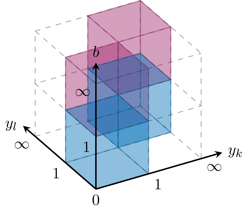
(a) $n\leftrightarrow\bar{n}$ exchange

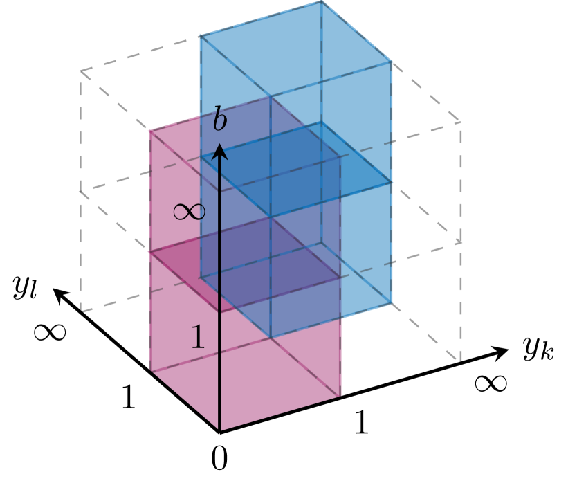
(b) $k\leftrightarrow l$ exchange

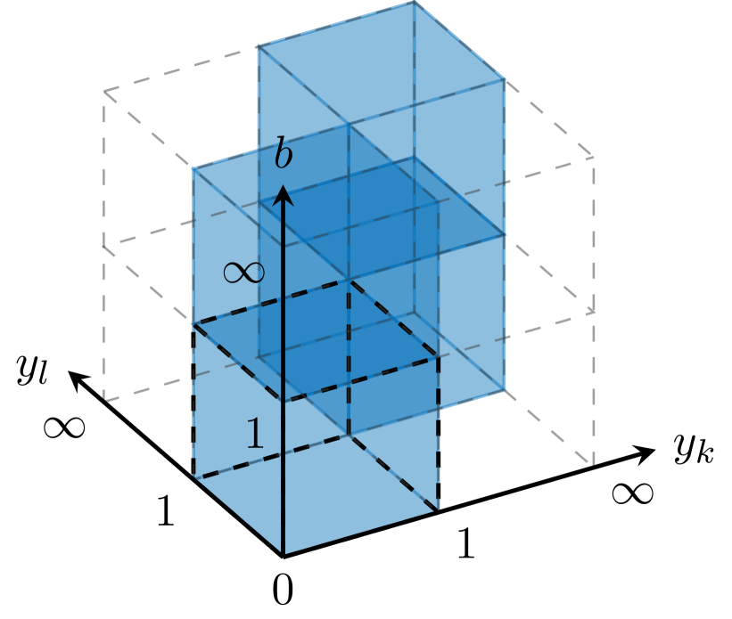
(c) Reduced integration region

Figure 1: Reduction of the integration domain in the variables $y_{k}$, $y_{l}$ and $b$ for the uncorrelated-emission contribution. Cubes of the same colour correspond to integration regions which yield the same result according to the stated symmetries. The second integration region B, complementing the highlighted region A in (c), can be any of the white adjacent cubes. In practice it is most easily recovered from A by inverting either $y_{k}$ or $y_{l}$.

After performing all of these manipulations, we arrive at the following master formula for the calculation of the uncorrelated-emission contribution

$$S_{RR}^{(C_{F})}(\epsilon,\alpha)=\frac{128C_{F}^{2}\,e^{-2\gamma_{E}(\epsilon+\alpha)}\,\Gamma(-4\epsilon-2\alpha)}{\pi^{3/2}\,\Gamma(-\epsilon)\,\Gamma(1/2-\epsilon)}\;\int_{0}^{1}\!dy_{k}\int_{0}^{1}\!dy_{l}\int_{0}^{1}\!db\int_{0}^{1}\!dt_{kl}\int_{0}^{1}\!dt_{l}\int_{0}^{1}\!dt_{5}^{\prime}$$

$$\qquad\times b^{-1-2\epsilon-\alpha}\,(y_{k}y_{l})^{-1+n\epsilon+(n+1)\alpha/2}\,(1+b)^{4\epsilon+2\alpha}\;\big{[}(1+y_{k})(1+y_{l})\big{]}^{2n\epsilon+(n-1)\alpha}$$

$$\qquad\times\big{(}4t_{kl}\bar{t}_{kl}\big{)}^{-1/2-\epsilon}\;\big{(}4t_{l}\bar{t}_{l}\big{)}^{-1/2-\epsilon}\;\big{(}t_{5}^{\prime}(2-t_{5}^{\prime})\big{)}^{-1-\epsilon}\;$$

$$\qquad\times\Big{\{}G_{A}(y_{k},y_{l},b,t_{k}^{+},t_{l},t_{kl})^{4\epsilon+2\alpha}+G_{B}(y_{k},y_{l},b,t_{k}^{+},t_{l},t_{kl})^{4\epsilon+2\alpha}+(t_{k}^{+}\to t_{k}^{-})\Big{\}}$$ (23)

with

$$t_{k}^{\pm}=t_{l}+t_{kl}-2t_{l}t_{kl}\pm 2\sqrt{t_{l}\bar{t}_{l}t_{kl}\bar{t}_{kl}}\,(1-t_{5}^{\prime})$$ (24)

and

$$G_{A}(y_{k},y_{l},b,t_{k},t_{l},t_{kl}) =G(y_{k},y_{l},b,t_{k},t_{l},t_{kl})\,,$$

$$G_{B}(y_{k},y_{l},b,t_{k},t_{l},t_{kl}) =\begin{dcases}\,y_{k}^{-n}\;G(1/y_{k},y_{l},b,t_{k},t_{l},t_{kl})&\,\text{or}\\ \,y_{l}^{-n}\;G(y_{k},1/y_{l},b,t_{k},t_{l},t_{kl})\,.\end{dcases}$$ (25)

In physical terms region A describes the emission of two soft partons into the same hemisphere with respect to the collinear axis, whereas region B covers the opposite-hemisphere case. Similar to Bell:2018oqa , the expression in region B is not unique, since the symmetry arguments only guarantee that the integrals in (23) are equal, but not necessarily the integrands. One is therefore free to derive the functional form of $G_{B}$ using either of the expressions on the right-hand side of (25).

From (23) we can analyse the divergence structure of the uncorrelated-emission contribution. For SCET-1 observables with $n\neq 0$, one can set the analytic regulator $\alpha$ to zero, and one finds an explicit divergence encoded in $\Gamma(-4\epsilon)$ that originates from the analytic integration over the dimensionful variable $q_{T}$. The integrand is, moreover, divergent in the limits $b\to 0$, $y_{k}\to 0$ and $y_{l}\to 0$ as anticipated in Section 2. In addition, there exists a spurious divergence in the limit $t_{5}^{\prime}\to 0$, which is cancelled by the prefactor $1/\Gamma(-\epsilon)$ as in Bell:2018oqa . The overall contribution to the bare soft function therefore starts with a $1/\epsilon^{4}$ divergence for SCET-1 observables.

For SCET-2 soft functions with $n=0$, the analytic regulator cannot be set to zero, since the $y_{k}$ and $y_{l}$-integrations generate poles in $\alpha$ in this case. As the $\alpha$-expansion has to be performed first, the terms $b^{-1-2\epsilon-\alpha}$ and $\Gamma(-4\epsilon-2\alpha)$ introduce additional $\epsilon$-divergences, and they trade $\alpha$-poles for $\epsilon$-poles in the double expansion. The leading divergences in the SCET-2 case are therefore of the form $1/(\alpha^{2}\epsilon^{2})$, $1/(\alpha\epsilon^{3})$ and $1/\epsilon^{4}$.

Finally, we noted towards the end of Section 2 that the collinear limits $y_{k}\to 0$ and $y_{l}\to 0$ can be ambiguous on the observable level. In order to disentangle the joint collinear limit of the emitted partons from the individual ones, we apply a sector decomposition strategy in the same-hemisphere contribution and write

$$\int_{0}^{1}\!dy_{k}\,\int_{0}^{1}\!dy_{l}\;\;\mathcal{I}(y_{k},y_{l}) =\int_{0}^{1}\!dy\,\int_{0}^{1}\!dr\;y\;\bigg{\{}\mathcal{I}(y,ry)+\mathcal{I}(ry,y)\bigg{\}}\,,$$ (26)

where $\mathcal{I}(y_{k},y_{l})$ symbolically represents the integrand in (23), which implicitly depends on the other integration variables. This generates two subregions in region A with

$$G_{A_{1}}(y,r,b,t_{k},t_{l},t_{kl}) =G_{A}(y,ry,b,t_{k},t_{l},t_{kl})\,,$$

$$G_{A_{2}}(y,r,b,t_{k},t_{l},t_{kl}) =G_{A}(ry,y,b,t_{k},t_{l},t_{kl})\,.$$ (27)

In the numerical implementation of our algorithm we perform a number of additional substitutions that are designed to improve the numerical convergence. For more details on this technical point we refer to Section 6 of Bell:2018oqa and the SoftSERVE user manual.

4 Renormalisation

With the master formula of the uncorrelated-emission contribution at hand, we have assembled all ingredients required for the calculation of bare NNLO dijet soft functions. In Bell:2018oqa we went one step ahead and extracted the anomalous dimensions and matching corrections that are needed for resummations within SCET. To do so, we assumed that the renormalised soft function $S=Z_{S}S_{0}$ obeys the renormalisation group equation (RGE)

$$\frac{\mathrm{d}}{\mathrm{d}\ln\mu}\;S(\tau,\mu) =-\frac{1}{n}\,\bigg{[}4\,\Gamma_{\mathrm{cusp}}(\alpha_{s})\,\ln(\mu\bar{\tau})-2\gamma^{S}(\alpha_{s})\bigg{]}\;S(\tau,\mu)$$ (28)

for SCET-1 observables, whereas we focused on the collinear anomaly exponent $\mathcal{F}(\tau,\mu)$ defined via

$$S(\tau,\mu,\nu) =(\nu^{2}\bar{\tau}^{2})^{-\mathcal{F}(\tau,\mu)}\;W^{S}(\tau,\mu)$$ (29)

in the SCET-2 case. The calculations provided in the current paper are fully compatible with this setup, and they provide the $C_{F}^{2}$ coefficients of the anomalous dimensions and matching corrections that were derived in Bell:2018oqa on the basis of NAE.

In this paper we generalise the renormalisation programme in two respects. First, we consider soft functions that renormalise directly in momentum (or cumulant) space rather than Laplace space, which is relevant e.g. for certain jet-veto observables. Second, we discuss the renormalisation of SCET-2 soft functions in the RRG approach Chiu:2012ir , which is equivalent to the collinear anomaly framework from Becher:2010tm ; Becher:2011pf , but which requires a specific implementation of the rapidity regulator. We will address both of these questions in turn.

4.1 Cumulant soft functions

Soft functions for jet-veto observables typically involve measurement functions that are formulated in terms of a $\theta$-function, which reflects the fact that the jet veto provides a cutoff for the phase-space integrations of the soft radiation. Instead of the exponential form (2), their measurement function can be expressed as

$$\widehat{\mathcal{M}}(\omega;\{k_{i}\})=\theta\big{(}\omega-\omega(\{k_{i}\})\,\big{)}\,,$$ (30)

where $\omega$ is the cutoff variable and the function $\omega(\{k_{i}\})$ is assumed to obey the same constraints that were listed in detail in Section 2.

The measurement function of such cumulant soft functions can easily be brought into the form (2) via a Laplace transformation,

$$\int_{0}^{\infty}\text{d}\omega\;e^{-\tau\omega}\;\theta\big{(}\omega-\omega(\{k_{i}\})\,\big{)} =\frac{1}{\tau}\;\exp\big{(}-\tau\,\omega(\{k_{i}\})\,\big{)}\,.$$ (31)

The factor $1/\tau$ is just a constant for the bare soft function calculation, but it is relevant for inverting the Laplace transformation. From (18) we see that the individual contributions to the soft function come with different powers of the Laplace variable $\tau$, which can be transformed back to momentum space using the relation

$$\int_{0}^{\infty}\text{d}\omega\;e^{-\tau\omega}\;\omega^{m} =\Gamma(1+m)\;\tau^{-1-m}\,,\qquad m>-1\,.$$ (32)

Up to NNLO a generic bare cumulant soft function therefore takes the form

$$\widehat{S}_{0}(\omega,\nu)=1 +\left(\frac{Z_{\alpha}\alpha_{s}}{4\pi}\right)\left(\frac{\mu^{2}}{\omega^{2}}\right)^{\epsilon}\left(\frac{\nu}{\omega}\right)^{\alpha}\frac{e^{\gamma_{E}(2\epsilon+\alpha)}}{\Gamma(1-2\epsilon-\alpha)}\;S_{R}(\epsilon,\alpha)$$ (33)

$$+\left(\frac{Z_{\alpha}\alpha_{s}}{4\pi}\right)^{2}\left(\frac{\mu^{2}}{\omega^{2}}\right)^{2\epsilon}\,\bigg{\{}\left(\frac{\nu}{\omega}\right)^{\alpha}\frac{e^{\gamma_{E}(4\epsilon+\alpha)}}{\Gamma(1-4\epsilon-\alpha)}\;S_{RV}(\epsilon,\alpha)$$

$$\hskip 113.81102pt+\left(\frac{\nu}{\omega}\right)^{2\alpha}\frac{e^{\gamma_{E}(4\epsilon+2\alpha)}}{\Gamma(1-4\epsilon-2\alpha)}\;S_{RR}(\epsilon,\alpha)\bigg{\}}+\mathcal{O}(\alpha_{s}^{3})\,,$$

where the terms $S_{i}(\epsilon,\alpha)$ for $i\in\{R,RV,RR\}$ can be calculated with the formulae provided in Bell:2018oqa and the present paper, and their prefactors in terms of Euler’s constant and Gamma functions slightly reshuffle the coefficients in the $\epsilon$ and $\alpha$ expansions. They do not modify, however, the divergence structure of the soft function since they all expand to $1+\mathcal{O}(\alpha,\epsilon)$.

We now assume that the RGEs for cumulant soft functions take the same form as (28) and the corresponding equation in the SCET-2 case, with the replacement $\bar{\tau}\to 1/\omega$. The renormalisation procedure that we developed for Laplace-space soft functions in Bell:2018oqa can then be carried over to cumulant soft functions if the prefactors in (33) are included. As we will explain later in Section 5, SoftSERVE 1.0 contains a script for the renormalisation of cumulant soft functions which applies these modifications and which takes the correct error propagation into account.

4.2 Rapidity renormalisation group

The collinear anomaly Becher:2010tm ; Becher:2011pf and the RRG Chiu:2012ir provide two equivalent frameworks for the renormalisation of SCET-2 soft functions. In the latter the soft function is renormalised via multiplication with a Z-factor, $S=Z_{S}S_{0}$, that absorbs the divergences both in the dimensional regulator $\epsilon$ and the rapidity regulator $\alpha$. The renormalised soft function is furthermore assumed to satisfy the RRG equation

$$\frac{\mathrm{d}}{\mathrm{d}\ln\nu}\;S(\tau,\mu,\nu) =\bigg{[}4\,A_{\Gamma}(\mu_{s},\mu)-2\gamma_{\nu}^{S}(\tau,\mu_{s})\bigg{]}\;S(\tau,\mu,\nu)\,,$$ (34)

where $A_{\Gamma}(\mu_{1},\mu_{2})$ is an RG kernel that was given explicitly in Bell:2018oqa , and the $\nu$-anomalous dimension can be identified with the collinear anomaly exponent defined in (29) via

$$\gamma_{\nu}^{S}(\tau,\mu_{s}) =\mathcal{F}(\tau,\mu_{s})\,.$$ (35)

In the RRG approach the renormalised soft function is in addition supposed to obey a RGE in the scale $\mu$,

$$\frac{\mathrm{d}}{\mathrm{d}\ln\mu}\;S(\tau,\mu,\nu) =\bigg{[}4\,\Gamma_{\mathrm{cusp}}(\alpha_{s})\,\ln(\mu\bar{\tau})-4\,\Gamma_{\mathrm{cusp}}(\alpha_{s})\,\ln(\nu\bar{\tau})-2\gamma^{S}_{\mu}(\alpha_{s})\bigg{]}\;S(\tau,\mu,\nu)\,,$$ (36)

whereas the corresponding quantity in the collinear anomaly framework – the soft remainder function $W^{S}(\tau,\mu)$ in (29) – does not obey a simple RGE without its collinear counterpart. The RRG therefore makes stronger assumptions than the collinear anomaly framework, and we argued in Bell:2018oqa that the RGE (36) only holds if the rapidity regulator is implemented on the level of connected webs – a necessary requirement for the consistency of the RRG approach that was not formulated so clearly in the original literature.

As we implement the rapidity regulator via the prescription (17) for individual emissions, our default setup is not suited for the RRG approach. In other words the $\alpha^{0}$-pieces calculated with SoftSERVE 0.9 cannot be renormalised in a way that is consistent with (36) (as the problem does not affect the $1/\alpha$ poles, all results presented in Bell:2018vaa ; Bell:2018oqa ; Bell:2018jvf are nevertheless correct). In SoftSERVE 1.0 we remedy this point and implement an alternative prescription that fulfils the requirements of the RRG approach. To do so, we add a factor $w^{2}$ to (17), where $w$ is a bookkeeping parameter that fulfils the RRG equation $\mathrm{d}w/\mathrm{d}\ln\nu=-\alpha w/2$ Chiu:2012ir , and we implement the rapidity regulator for double correlated emissions via

$$w^{2}\,\int d^{d}k\int d^{d}l\;\left(\frac{\nu}{k_{+}+k_{-}+l_{+}+l_{-}}\right)^{\alpha}\;\delta(k^{2})\theta(k^{0})\;\delta(l^{2})\theta(l^{0})$$ (37)

rather than

$$w^{4}\int d^{d}k\;\left(\frac{\nu}{k_{+}+k_{-}}\right)^{\alpha}\;\delta(k^{2})\theta(k^{0})\;\int d^{d}l\;\left(\frac{\nu}{l_{+}+l_{-}}\right)^{\alpha}\;\delta(l^{2})\theta(l^{0})\,,$$ (38)

whereas the remaining contributions to the bare soft function are not changed, except for trivial factors of $w$.

We will address the technical aspects of the SoftSERVE implementation in the following section, and show here how to extract the two-loop anomalous dimensions and matching corrections from the bare soft function in the RRG setup. To do so, we start from

$$S_{0}(\tau,\nu) =1+\left(\frac{Z_{\alpha}\alpha_{s}}{4\pi}\right)\,w^{2}\,(\mu^{2}\bar{\tau}^{2})^{\epsilon}\;(\nu\bar{\tau})^{\alpha}\bigg{\{}\frac{1}{\alpha}\bigg{(}\frac{x^{1}_{1}}{\epsilon}+x^{1}_{0}+x^{1}_{-1}\,\epsilon+x^{1}_{-2}\,\epsilon^{2}+x^{1}_{-3}\,\epsilon^{3}\bigg{)}$$ (39)

$$+\frac{x^{0}_{2}}{\epsilon^{2}}+\frac{x^{0}_{1}}{\epsilon}+x^{0}_{0}+x^{0}_{-1}\,\epsilon+x^{0}_{-2}\,\epsilon^{2}+\alpha\bigg{(}\frac{x^{-1}_{3}}{\epsilon^{3}}+\frac{x^{-1}_{2}}{\epsilon^{2}}+\frac{x^{-1}_{1}}{\epsilon}+x^{-1}_{0}+x^{-1}_{-1}\,\epsilon\bigg{)}$$

$$+\mathcal{O}\Big{(}\frac{\epsilon^{4}}{\alpha},\epsilon^{3},\alpha\epsilon^{2},\alpha^{2}\Big{)}\bigg{\}}+\left(\frac{Z_{\alpha}\alpha_{s}}{4\pi}\right)^{2}(\mu^{2}\bar{\tau}^{2})^{2\epsilon}\;\bigg{\{}w^{4}\,(\nu\bar{\tau})^{2\alpha}\,\bigg{[}\frac{1}{\alpha^{2}}\bigg{(}\frac{y^{2}_{2}}{\epsilon^{2}}+\frac{y^{2}_{1}}{\epsilon}+y^{2}_{0}\bigg{)}$$

$$+\frac{1}{\alpha}\bigg{(}\frac{y^{1}_{3}}{\epsilon^{3}}+\frac{y^{1}_{2}}{\epsilon^{2}}+\frac{y^{1}_{1}}{\epsilon}+y^{1}_{0}\bigg{)}+\frac{y^{0}_{4}}{\epsilon^{4}}+\frac{y^{0}_{3}}{\epsilon^{3}}+\frac{y^{0}_{2}}{\epsilon^{2}}+\frac{y^{0}_{1}}{\epsilon}+y^{0}_{0}+\mathcal{O}\Big{(}\frac{\epsilon}{\alpha^{2}},\frac{\epsilon}{\alpha},\epsilon,\alpha\Big{)}\bigg{]}$$

$$+w^{2}\,(\nu\bar{\tau})^{\alpha}\bigg{[}\frac{1}{\alpha}\bigg{(}\frac{z^{1}_{3}}{\epsilon^{3}}+\frac{z^{1}_{2}}{\epsilon^{2}}+\frac{z^{1}_{1}}{\epsilon}+z^{1}_{0}\bigg{)}+\frac{z^{0}_{4}}{\epsilon^{4}}+\frac{z^{0}_{3}}{\epsilon^{3}}+\frac{z^{0}_{2}}{\epsilon^{2}}+\frac{z^{0}_{1}}{\epsilon}+z^{0}_{0}+\mathcal{O}\Big{(}\frac{\epsilon}{\alpha},\epsilon,\alpha\Big{)}\bigg{]}\bigg{\}},$$

where the only difference with respect to Bell:2018oqa consists in the presence of the bookkeeping parameter $w$. Due to (37) the correlated-emission contribution is, moreover, now contained in the $z^{i}_{j}$ coefficients along with the real-virtual interference term. The single real-emission and uncorrelated double-emission contributions constitute the $x^{i}_{j}$ and $y^{i}_{j}$ coefficients, respectively, as before. The coefficients $x^{i}_{j}$ are thus proportional to the colour factor $C_{F}$, the $y^{i}_{j}$ to $C_{F}^{2}$, and the $z^{i}_{j}$ consist of two contributions with colour factors $C_{F}T_{f}n_{f}$ and $C_{F}C_{A}$.

We now expand the anomalous dimensions to two-loop order,

$$\Gamma_{\mathrm{cusp}}(\alpha_{s}) =\left(\frac{\alpha_{s}}{4\pi}\right)\Gamma_{0}+\left(\frac{\alpha_{s}}{4\pi}\right)^{2}\Gamma_{1}\,,$$ (40)

$$\gamma_{\mu}^{S}(\alpha_{s}) =\left(\frac{\alpha_{s}}{4\pi}\right)\gamma^{S}_{\mu,0}+\left(\frac{\alpha_{s}}{4\pi}\right)^{2}\gamma^{S}_{\mu,1}\,,$$

$$\gamma_{\nu}^{S}(\tau,\mu) =\left(\frac{\alpha_{s}}{4\pi}\right)\Big{\{}2\Gamma_{0}L_{\mu}+\gamma^{S}_{\nu,0}\Big{\}}+\left(\frac{\alpha_{s}}{4\pi}\right)^{2}\Big{\{}2\beta_{0}\Gamma_{0}L_{\mu}^{2}+2\left(\Gamma_{1}+\beta_{0}\gamma^{S}_{\nu,0}\right)L_{\mu}+\gamma^{S}_{\nu,1}\Big{\}},$$

where $L_{\mu}=\ln(\mu\bar{\tau})$ and the coefficients $\gamma^{S}_{\nu,i}$ correspond to the $d_{i+1}$ in the collinear anomaly language of Bell:2018oqa . Using $Z_{\alpha}=1-\beta_{0}\alpha_{s}/(4\pi\epsilon)+\mathcal{O}(\alpha_{s}^{2})$, we can solve the RGEs (34) and (36) for the soft function and the corresponding equations for the Z-factor $Z_{S}=S/S_{0}$ explicitly. In order to avoid cross terms from higher orders, the latter is conveniently determined via its logarithm, which in the $\overline{\text{MS}}$ scheme takes the form

$$\ln Z_{S}=\left(\frac{\alpha_{s}}{4\pi}\right)w^{2}\,\bigg{\{}\frac{2\Gamma_{0}}{\alpha\epsilon}+\frac{4\Gamma_{0}L_{\mu}+2\gamma_{\nu,0}^{S}}{\alpha}-\frac{\Gamma_{0}}{\epsilon^{2}}+\frac{\gamma_{\mu,0}^{S}-2\Gamma_{0}(L_{\mu}-L_{\nu})}{\epsilon}\bigg{\}}$$

$$\quad+\left(\frac{\alpha_{s}}{4\pi}\right)^{2}w^{2}\,\bigg{\{}-\frac{\beta_{0}\Gamma_{0}}{\alpha\epsilon^{2}}+\frac{\Gamma_{1}}{\alpha\epsilon}+\Big{(}4\beta_{0}\Gamma_{0}L_{\mu}^{2}+4(\Gamma_{1}+\beta_{0}\gamma_{\nu,0}^{S})L_{\mu}+2(\gamma_{\nu,1}^{S})_{C}+w^{2}(\gamma_{\nu,1}^{S})_{U}\Big{)}\frac{1}{\alpha}$$

$$\hskip 79.66771pt+\frac{3\beta_{0}\Gamma_{0}}{4\epsilon^{3}}-\frac{1}{4}\Big{(}\Gamma_{1}+2\beta_{0}\gamma_{\mu,0}^{S}-4\beta_{0}\Gamma_{0}(L_{\mu}-L_{\nu})\Big{)}\frac{1}{\epsilon^{2}}$$

$$\hskip 79.66771pt-\frac{1}{2}\Big{(}2\Gamma_{1}(L_{\mu}-L_{\nu})-(\gamma_{\mu,1}^{S})_{C}-w^{2}(\gamma_{\mu,1}^{S})_{U}\Big{)}\frac{1}{\epsilon}\bigg{\}}\,,$$ (41)

where $L_{\nu}=\ln(\nu\bar{\tau})$ and we have split the correlated and uncorrelated-emission contributions to the two-loop anomalous dimensions $\gamma^{S}_{\mu,1}$ and $\gamma^{S}_{\nu,1}$ since – according to (39) – they come with different powers of the bookkeeping parameter $w$. For the renormalised soft function, we obtain up to the considered two-loop order

$$\ln S(\tau,\mu,\nu)=\left(\frac{\alpha_{s}}{4\pi}\right)\bigg{\{}2\Gamma_{0}L_{\mu}^{2}-4\Gamma_{0}L_{\mu}L_{\nu}-2\gamma^{S}_{\mu,0}L_{\mu}-2\gamma^{S}_{\nu,0}L_{\nu}+c_{1}^{S}\bigg{\}}$$

$$\quad+\left(\frac{\alpha_{s}}{4\pi}\right)^{2}\bigg{\{}\frac{4}{3}\beta_{0}\Gamma_{0}L_{\mu}^{3}-4\beta_{0}\Gamma_{0}L_{\mu}^{2}L_{\nu}+2\Big{(}\Gamma_{1}-\beta_{0}\gamma_{\mu,0}^{S}\Big{)}L_{\mu}^{2}-4\Big{(}\Gamma_{1}+\beta_{0}\gamma_{\nu,0}^{S}\Big{)}L_{\mu}L_{\nu}$$

$$\hskip 62.59605pt-2\Big{(}\gamma_{\mu,1}^{S}-\beta_{0}c_{1}^{S}\Big{)}L_{\mu}-2\gamma_{\nu,1}^{S}L_{\nu}+c_{2}^{S}-\frac{1}{2}(c_{1}^{S})^{2}\bigg{\}}\,,$$ (42)

where we have set $w=1$. As the cusp anomalous dimension and the beta function are known to the required order,

$$\Gamma_{0}=4C_{F}\,,\quad\Gamma_{1}=4C_{F}\left\{\left(\frac{67}{9}-\frac{\pi^{2}}{3}\right)C_{A}-\frac{20}{9}T_{F}n_{f}\right\},\quad\beta_{0}=\frac{11}{3}C_{A}-\frac{4}{3}T_{F}n_{f}\,,$$ (43)

the higher poles in the product of the Z-factor and the bare soft function provide checks of our calculation, whereas the coefficients of the $1/\alpha$ and $1/\epsilon$ poles determine the rapidity anomalous dimension $\gamma^{S}_{\nu}$ and the $\mu$-anomalous dimension $\gamma^{S}_{\mu}$, respectively. In terms of the coefficients introduced in (39), we obtain

$$\gamma^{S}_{\nu,0} =-\frac{x^{1}_{0}}{2}\,,$$

$$\gamma^{S}_{\nu,1} =-y^{1}_{0}-\frac{z^{1}_{0}}{2}+x^{0}_{-1}x^{1}_{1}+x^{0}_{0}x^{1}_{0}+x^{0}_{1}x^{1}_{-1}+x^{0}_{2}x^{1}_{-2}+\frac{\beta_{0}x^{1}_{-1}}{2}\,,$$ (44)

which is precisely the relation we found for the collinear anomaly exponent in Bell:2018oqa . The non-logarithmic terms of the renormalised soft function are, on the other hand, in the RRG framework given by

$$c_{1}^{S} =x^{0}_{0}\,,$$ (45)

$$c_{2}^{S} =y^{0}_{0}+z^{0}_{0}-x^{0}_{2}x^{0}_{-2}-(x^{0}_{1}+\beta_{0})x^{0}_{-1}-x^{1}_{1}x^{-1}_{-1}-x^{1}_{0}x^{-1}_{0}-x^{1}_{-1}x^{-1}_{1}-x^{1}_{-2}x^{-1}_{2}-x^{1}_{-3}x^{-1}_{3}\,,$$

whereas one can show that the $\mu$-anomalous dimension is unphysical for SCET-2 soft functions since it drops out in the final expressions once the soft and collinear RG kernels are combined. Following the procedure outlined in Bell:2018vaa , we can actually prove that the $\mu$-anomalous dimension is a universal number in our setup, i.e. it is independent of the observable given by

$$\gamma^{S}_{\mu,0}=0\,,\quad\gamma^{S}_{\mu,1}=\bigg{\{}\frac{224}{27}-\frac{4\pi^{2}}{9}\bigg{\}}\,C_{F}T_{F}n_{f}\,+\,\bigg{\{}-\frac{808}{27}+\frac{11\pi^{2}}{9}+28\zeta_{3}\bigg{\}}\,C_{F}C_{A}\,.$$ (46)

Rather than extracting this quantity from the coefficient of the $1/\epsilon$ pole, we therefore turn the argument around and use these numbers in SoftSERVE to check if the singularities cancel out as predicted by the RRG framework.

The discussion of cumulant soft functions from the previous section applies identically to the RRG setup, with the sole exception that the correlated-emission contribution in (33) comes with a prefactor $e^{\gamma_{E}(4\epsilon+\alpha)}/\Gamma(1-4\epsilon-\alpha)$ rather than $e^{\gamma_{E}(4\epsilon+2\alpha)}/\Gamma(1-4\epsilon-2\alpha)$ because of (37). Once again, SoftSERVE 1.0 provides a script that takes these modifications into account.

5 Extending the SoftSERVE distribution

The central new element of SoftSERVE 1.0 is the direct calculation of the uncorrelated-emission contribution, whereas SoftSERVE 0.9 reconstructs this term from the NLO correction, assuming that the observable is consistent with NAE. For the SoftSERVE user, this means that calling make all – or calling make without target – now generates executables for all colour structures, and the target list is supplemented with the uncorrelated, CFA and CFB targets. The latter correspond to the two contributions from regions A and B in (23), and uncorrelated refers to them as a pair. For observables obeying NAE, the correlated target now provides all the required input, skipping the $C_{F}^{2}$ contributions.

In addition we implemented the new features discussed in Section 4 concerning cumulant soft functions and the RRG. Apart from the existing script for the renormalisation of Laplace-space soft functions (laprenorm), there now also exists a script for the renormalisation of cumulant soft functions (momrenorm) that applies the changes discussed in Section 4.1. Both scripts come in two versions designed for observables that obey NAE (postfix NAE) and those that violate NAE (no postfix). The latter require the full set of results files, whereas the former do not need the CFA and CFB results – they reconstruct the $C_{F}^{2}$ contribution directly from the NLO result. Execution and summary scripts to run and refine the results now also exist in two versions for observables that obey/violate NAE, similarly postfixed. To prevent accidentally calling non-NAE scripts on results that are derived assuming NAE, some safeguards are implemented.

Moreover, the SCET-2 executables can now be generated with a rapidity regulator that is compatible with the RRG approach. As discussed in Section 4.2, this requires that one implements the regulator on the level of connected webs rather than individual emissions. At NNLO the only difference arises in the correlated-emission contribution for which the regulator is implemented via (37) rather than (38). This feature is switched off by default, but it can be used by setting a nonzero RRG variable during the make call. In other words, to generate e.g. the $C_{F}T_{F}n_{f}$ colour structure binary for some observable using the RRG regulator, one calls make NF RRG=1. In the SCET-2 branch, there are scripts to summarise (sftsrvres), renormalise (laprenorm or momrenorm) and to account for Fourier phases (fourierconvert) that use the results derived with the new regulator, and they are all postfixed RRG. These scripts of course also exist for observables that obey NAE, and they then simply carry both postfixes like laprenormNAERRG. Again, safeguards to avoid calling RRG scripts on results that were derived with the default rapidity regulator and vice-versa are implemented.

Finally, we added the formulae derived in Bell:2018vaa that allow for a direct calculation of the soft anomalous dimensions and collinear anomaly exponents without having to calculate the complete bare soft function. As the SoftSERVE input differs slightly from the conventions of Bell:2018vaa , we rederived these formulae in a form that is suitable for SoftSERVE and summarise the corresponding expressions in Appendix A. To access these formulae the user must call make with targets ADLap or ADMom, which generates the respective executables for Laplace-space and cumulant soft functions. These executables then reside in the Executables folder and must be called manually. While they allow for a fast evaluation of the anomalous dimension/anomaly exponent, we do not recommend using them for a precision determination since they are numerically less robust. Observables which exhibit features that reduce numerical accuracy, like integrable divergences, slow them down disproportionately. In addition, the term (63), which is conjectured to vanish for all observables, happens to sometimes be numerically unstable due to the peculiar structure in its last line. For observables for which this expression is non-trivial, the integration converges comparatively slowly.

6 Results

We are now in a position to use SoftSERVE 1.0 to compute NNLO dijet soft functions for various $e^{+}e^{-}$ event shapes and hadron-collider observables. As in Bell:2018oqa , we present our results for SCET-1 soft functions in the form

$$\gamma_{0}^{S} =\gamma_{0}^{C_{F}}\,C_{F}\,,$$

$$\gamma_{1}^{S} =\gamma_{1}^{C_{A}}\,C_{F}C_{A}+\gamma_{1}^{n_{f}}\,C_{F}T_{F}n_{f}+\gamma_{1}^{C_{F}}\,C_{F}^{2}\,,$$

$$c_{1}^{S} =c_{1}^{C_{F}}\,C_{F}\,,$$

$$c_{2}^{S} =c_{2}^{C_{A}}\,C_{F}C_{A}+c_{2}^{n_{f}}\,C_{F}T_{F}n_{f}+c_{2}^{C_{F}}\,C_{F}^{2}\,,$$ (47)

where the coefficients $\gamma^{S}_{i}$ of the soft anomalous dimension and the finite terms $c_{i}^{S}$ of the renormalised soft function refer to the conventions introduced in Section 4.1 of Bell:2018oqa . In contrast to that work, we now use SoftSERVE to calculate the $\gamma_{1}^{C_{F}}$ and $c_{2}^{C_{F}}$ numbers, which were derived in Bell:2018oqa on the basis of NAE.

For SCET-2 soft functions we quote our numbers in the RRG notation of Section 4.2. The relevant resummation ingredients are in this case the coefficients $\gamma_{\nu,i}^{S}$ of the rapidity anomalous dimension and the finite terms $c_{i}^{S}$ of the RRG renormalised soft function, which we decompose analogously to (47) according to their colour structures. Whereas the former are equivalent to the anomaly coefficients $d_{i+1}$ used in Bell:2018oqa , the latter are not well defined in the collinear anomaly framework and were therefore not given in Bell:2018oqa . As explained in Section 4.2, the $\mu$-anomalous dimension $\gamma_{\mu}^{S}$ is, moreover, unphysical for SCET-2 soft functions and will therefore be disregarded in the following.

Similar to Bell:2018oqa , SoftSERVE 1.0 comes with a number of template files that can be used to rederive the numbers quoted in this section. For most of the observables the runtime of the uncorrelated-emission contribution turns out to be comparable to the correlated-emission calculation, which can of course be tailored to the specific needs of the user by adjusting the respective Cuba settings. Although the focus of the present paper is on NAE-violating observables, we first consider a few observables that respect NAE, since this allows us to test the new algorithm and to gauge the accuracy of our numerical predictions. We then switch to some exemplary NAE-violating soft functions in a second step.

6.1 Observables that obey NAE

For all observables in this section NAE implies $\gamma_{1}^{C_{F}}=0$ and $c_{2}^{C_{F}}=1/2(c_{1}^{C_{F}})^{2}$ for SCET-1 soft functions, and similarly $\gamma_{\nu,1}^{C_{F}}=0$ and $c_{2}^{C_{F}}=1/2(c_{1}^{C_{F}})^{2}$ in the SCET-2 case.

C-parameter

We first consider the C-parameter event shape, which was one of the template observables we studied in Bell:2018oqa . The only new element required for the uncorrelated-emission contribution is the function

$$G(y_{k},y_{l},b) =\frac{1}{(1+y_{k})(1+y_{l})}$$ (48)

defined in (9), which can be translated into the relevant input functions $G_{A_{1}}$, $G_{A_{2}}$ and $G_{B}$ using the relations (25) and (27). We then find using SoftSERVE 1.0

$$\gamma_{0}^{C_{F}} =1\cdot 10^{-10}\pm 2\cdot 10^{-7}\, \quad[0]\,, \qquad\quad c_{1}^{C_{F}} =-3.28987\pm 9\cdot 10^{-7}\, \quad[-3.28987]\,,$$

$$\gamma_{1}^{C_{A}} =15.7940(10)\, \quad[15.7945]\,, c_{2}^{C_{A}} =-57.9814(35) \quad[-57.9757]\,,$$

$$\gamma_{1}^{n_{f}} =3.90983(14)\, \quad[3.90981]\,, c_{2}^{n_{f}} =43.8181(4)\, \quad[43.8182]\,,$$

$$\gamma_{1}^{C_{F}} =-0.0004(24) \quad[0]\,, c_{2}^{C_{F}} =5.41178(592) \quad[5.41162]\,,$$ (49)

which is in excellent agreement with the analytic results from Hoang:2014wka ; Bell:2018oqa shown in the square brackets.

W-production at large transverse momentum

We next consider the soft function for $W$-production at large transverse momentum which we also discussed in detail in Bell:2018oqa . We now have

$$G(y_{k},y_{l},b,t_{k},t_{l},t_{kl}) \!=\!\frac{b(1+y_{l})(1+y_{k}-2\sqrt{y_{k}}(1-2t_{k}))}{(1+b)}+\frac{(1+y_{k})(1+y_{l}-2\sqrt{y_{l}}(1-2t_{l}))}{(1+b)}$$ (50)

and obtain

$$\gamma_{0}^{C_{F}} =-1\cdot 10^{-9}\pm 2\cdot 10^{-6}\, \quad[0]\,, \qquad\quad c_{1}^{C_{F}} =9.86960(2)\, \quad[9.86960]\,,$$

$$\gamma_{1}^{C_{A}} =15.7945(24)\, \quad[15.7945]\,, c_{2}^{C_{A}} =-2.64324(890) \quad[-2.65010]\,,$$

$$\gamma_{1}^{n_{f}} =3.90987(22)\, \quad[3.90981]\,, c_{2}^{n_{f}} =-25.3069(10)\, \quad[-25.3073]\,,$$

$$\gamma_{1}^{C_{F}} =-1\cdot 10^{-7}\pm 0.003 \quad[0]\,, c_{2}^{C_{F}} =48.7050(96) \quad[48.7045]\,,$$ (51)

which is again in perfect agreement with the analytic results from Becher:2012za .

Jet broadening

In order to illustrate the new RRG routine of SoftSERVE, we consider the SCET-2 event-shape variable jet broadening. As in Bell:2018oqa we consider a recoil-free definition here and refer to that paper for more details on the observable. The relevant input for the uncorrelated-emission contribution is then given by

$$G(y_{k},y_{l},b) =\frac{1}{2}\,,$$ (52)

which yields

$$\gamma_{\nu,0}^{C_{F}} =-5.54518(1) \quad[-5.54518]\,, \qquad\quad c_{1}^{C_{F}} =-20.2930(1) \quad[-20.2930]\,,$$

$$\gamma_{\nu,1}^{C_{A}} =7.03652(110) \quad[7.03605]\,, c_{2}^{C_{A}} =-56.6537(21)\,,$$

$$\gamma_{\nu,1}^{n_{f}} =-11.5393(1) \quad[-11.5393]\,, c_{2}^{n_{f}} =24.1971(3)\,,$$

$$\gamma_{\nu,1}^{C_{F}} =-0.00001(163) \quad[0]\,, c_{2}^{C_{F}} =205.902(5) \quad[205.902]\,.$$ (53)

For the rapidity anomalous dimension, this agrees with the expressions found in Becher:2012qc , and the one-loop matching coefficient $c_{1}^{C_{F}}=-8\ln^{2}2-5\pi^{2}/3$ can be extracted from that paper as well. Our results for the two-loop coefficients $c_{2}^{C_{A}}$ and $c_{2}^{n_{f}}$ are, on the other hand, new.

Transverse-momentum resummation

We finally examine the soft function for transverse-momentum resummation in Drell-Yan production, which is an example of a Fourier-space rather than a Laplace-space soft function. As argued in Bell:2018oqa , these can be computed with SoftSERVE by using the absolute value of the naive measurement function, which in the specific case of transverse-momentum resummation is given by

$$G(y_{k},y_{l},b,t_{k},t_{l},t_{kl}) =\frac{2}{1+b}\;\big{|}b(1-2t_{k})+1-2t_{l}\big{|}\,.$$ (54)

Running the fourierconvertRRG script before renormalisation, we then obtain

$$\gamma_{\nu,0}^{C_{F}} =1\cdot 10^{-9}\pm 2\cdot 10^{-6} \quad[0]\,, \qquad\quad c_{1}^{C_{F}} =-3.2899(1) \quad[-3.2899]\,,$$

$$\gamma_{\nu,1}^{C_{A}} =-3.7407(94) \quad[-3.7317]\,, c_{2}^{C_{A}} =-16.749(169) \quad[-16.507]\,,$$

$$\gamma_{\nu,1}^{n_{f}} =-8.2963(20) \quad[-8.2963]\,, c_{2}^{n_{f}} =10.338(27) \quad[10.347]\,,$$

$$\gamma_{\nu,1}^{C_{F}} =-0.0322(281) \quad[0]\,, c_{2}^{C_{F}} =5.1718(3987) \quad[5.4116]\,.$$ (55)

While we already calculated the rapidity anomalous dimension for this observable in Bell:2018oqa , we did not have access to the finite terms in the RRG framework at the time, which are however known analytically from the calculation in Luebbert:2016itl . Our SoftSERVE numbers compare well to these results, although we observe a slightly reduced accuracy in comparison to the prior examples, which is due to integrable divergences in the bulk of the integration region as well as the required Fourier shuffle, which mixes coefficients and adds up the corresponding errors. The agreement is, however, still acceptable.

6.2 Observables that violate NAE

Having established that SoftSERVE 1.0 satisfactorily reproduces known results for sample NAE observables, we now turn to soft functions that do not respect the NAE theorem and which require an independent calculation of the uncorrelated-emission contribution. Whereas we already presented our results for the corresponding anomalous dimensions in Bell:2018vaa ; Bell:2018jvf , we compute the matching coefficients in this work for the first time.

Rapidity-dependent jet vetoes

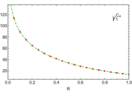
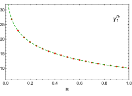
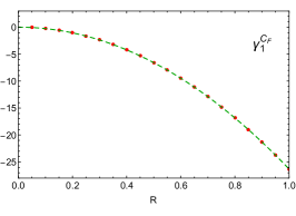
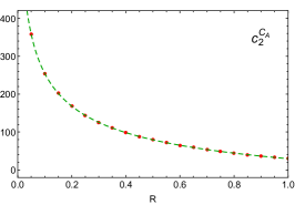
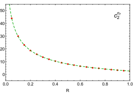
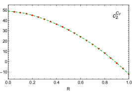
Figure 2: Two-loop anomalous dimension and finite term of the renormalised C-parameter jet-veto soft function. Red dots indicate values calculated with SoftSERVE and green dashed lines represent the interpolating functions from Gangal:2016kuo .

The first family of NAE-violating observables are the rapidity-dependent jet vetoes from Gangal:2014qda . Specifically, we consider the beam-thrust and C-parameter-like jet-veto variables $\mathcal{T}_{B\rm cm}$ and $\mathcal{T}_{C\rm cm}$ defined in that paper, which are both SCET-1 observables with $n=1$. For the C-parameter jet veto, one further has $f(y_{k},t_{k})=1/(1+y_{k})$ and

$$F(a,b,y,t_{k},t_{l},t_{kl}) =\theta(\Delta_{F}-R)\;\text{max}\bigg{(}\frac{ab}{a(a+b)+(1+ab)y}~{},~{}\frac{a}{a+b+a(1+ab)y}\bigg{)}$$

$$\quad+\theta(R-\Delta_{F})\;\frac{1}{1+y}\,,$$ (56)

where $R$ is the jet radius and $\Delta_{F}=\sqrt{\ln^{2}a+\arccos^{2}(1-2t_{kl})}$, and the corresponding expression for the uncorrelated-emission measurement function was given in (10). The jet-veto observables renormalise multiplicatively in cumulant space, and therefore the formalism from Section 4.1 applies in this case. Furthermore, as the jet algorithm has no effect on a single emission, the NLO coefficients $\gamma_{0}^{C_{F}}=0$ and $c_{1}^{C_{F}}=\pi^{2}$ are independent of the jet radius $R$, whereas the NNLO coefficients are displayed in the range $0\leq R\leq 1$ in Figure 2. From the plots it is evident that our SoftSERVE numbers agree well with the numerical results from Gangal:2016kuo indicated by the dashed lines.

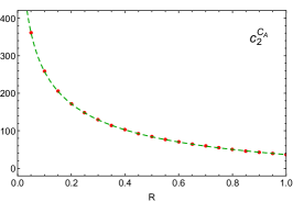
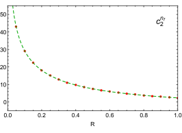
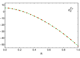
Figure 3: The same as in Figure 2 for the finite term of the renormalised beam-thrust jet-veto soft function.

For the beam-thrust jet veto, the input functions are slightly more complicated and we refer to the SoftSERVE manual for their explicit expressions. As the two jet vetoes have the same anomalous dimension, we refrain from showing the corresponding plots in this case, since they are – in view of the negligible numerical uncertainties – literally identical to the upper plots in Figure 2. The one-loop matching coefficient is, moreover, now given by $c_{1}^{C_{F}}=\pi^{2}/3$, and the two-loop coefficients are displayed as a function of the jet radius in Figure 3. Our numbers are once more in perfect agreement with the results from Gangal:2016kuo .

Standard jet veto

The standard way of implementing a jet veto uses a cutoff on the transverse momenta of the emissions. The corresponding soft function is in this case defined in SCET-2, and the required SoftSERVE input is given by $n=0$, $f(y_{k},t_{k})=1$ and

$$F(a,b,y,t_{k},t_{l},t_{kl}) =\sqrt{\frac{a}{(1+ab)(a+b)}}\bigg{\{}\!\theta(\Delta_{F}-R)+\theta(R-\Delta_{F})\sqrt{1+b^{2}+2b(1-2t_{kl})}\bigg{\}}\,,$$

$$\!\!\!\!G(y_{k},y_{l},b,t_{k},t_{l},t_{kl}) =\theta(\Delta_{G}-R)\,\frac{\max(1,b)}{1+b}+\theta(R-\Delta_{G})\,\frac{\sqrt{1+b^{2}+2b(1-2t_{kl})}}{1+b}\,.$$ (57)

As for the rapidity-dependent jet vetoes, the soft function renormalises multiplicatively in cumulant space, and the respective NLO coefficients are now given by $\gamma_{\nu,0}^{C_{F}}=0$ and $c_{1}^{C_{F}}=-\pi^{2}/3$. Our numbers for the two-loop rapidity anomalous dimension are shown in the upper plots of Figure 4, and they confirm the existing results from Banfi:2012yh ; Becher:2013xia ; Stewart:2013faa indicated by the dashed lines. In the RRG setup the two-loop matching corrections can furthermore be compared to Stewart:2013faa , which gives these numbers in an expansion in $R\ll 1$ up to terms of $\mathcal{O}(R^{0})$. As is evident from the lower plots in Figure 4, this expansion works surprisingly well for the $c_{2}^{C_{A}}$ and $c_{2}^{n_{f}}$ coefficients even for large values $R\simeq 1$, but it misses the leading $\mathcal{O}(R^{2})$ correction to $c_{2}^{C_{F}}$.

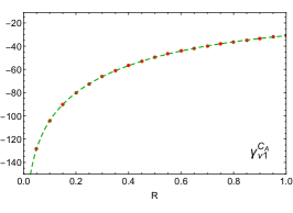
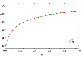
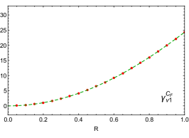
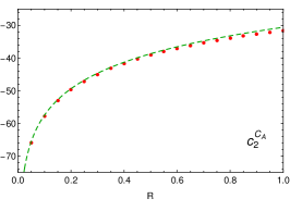
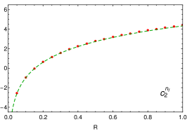
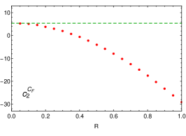
Figure 4: Two-loop rapidity anomalous dimension and finite term of the RRG renormalised $p_{T}$ veto soft function. Red dots indicate values calculated with SoftSERVE and green dashed lines show the interpolating functions from Becher:2013xia (upper plots) and Stewart:2013faa (lower plots).

Soft-drop jet groomer

Finally, we present novel results for the soft-drop groomed jet mass discussed in Frye:2016aiz . According to this definition, the groomer depends on a parameter $\beta$, and for values $\beta>0$ considered here, the soft function is defined in SCET-1 with $n=-1-\beta$. As the formulae for the measurement functions are rather lengthy, we refer to the SoftSERVE distribution for their explicit expressions. The renormalisation of the soft function is, moreover, again performed in cumulant space, and the one-loop coefficients are found to be $\gamma_{0}^{C_{F}}=0$ and $c_{1}^{C_{F}}=-\pi^{2}(3+3\beta+\beta^{2})/3/(1+\beta)$. Our results for the two-loop coefficients are shown in Figure 5 together with the numbers from Frye:2016aiz for the anomalous dimension. For $\beta=0$ these values have been extracted from an analytic calculation, whereas the $\beta=1$ numbers stem from a fit to the EVENT2 generator. From the plots we see that our results confirm these numbers, but they are far more precise than the EVENT2 extraction. Our results for other values of the grooming parameter $\beta$ are new, as are the finite terms of the renormalised soft function which are shown in the lower plots of the figure. Our numbers have actually already been used to extend the resummation for the soft-drop groomed jet mass to next-to-next-to-next-to-leading logarithmic (N³LL) accuracy Kardos:2020gty ; Kardos:2020ppl .

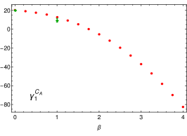
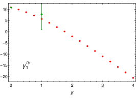
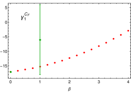
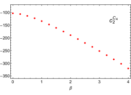
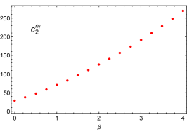
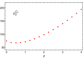
Figure 5: Two-loop anomalous dimensions and finite term of the renormalised soft function for the soft-drop jet groomer. Red dots indicate values calculated with SoftSERVE and the green diamonds show the numbers from Frye:2016aiz .

7 Conclusions

We have extended our automated approach for calculating NNLO dijet soft functions to the uncorrelated-emission ($C_{F}^{2}$) contribution. While one can trivially obtain this term from the NLO calculation for observables that obey the NAE theorem, one must calculate it explicitly for NAE-violating observables like those that depend on a jet algorithm. From the technical point of view, the divergence structure of the $C_{F}^{2}$ matrix element differs from the other colour structures treated in Bell:2018oqa , and we have devised a novel phase-space parametrisation that isolates these singularities.

Our algorithm permits a systematic numerical evaluation of NNLO dijet soft functions, and it is implemented in SoftSERVE 1.0 which we release alongside of this paper at https://softserve.hepforge.org/. In addition to the new core routine for calculating the uncorrelated-emission contribution to bare dijet soft functions, SoftSERVE 1.0 includes novel renormalisation scripts that are compatible with the RRG formalism and observables that renormalise directly in momentum space rather than Laplace space.

SoftSERVE has therefore become a powerful program for calculating NNLO dijet soft functions, and we have used it to cross-check existing calculations for multiple $e^{+}e^{-}$ and hadron-collider observables, as well as to obtain some novel predictions. In particular, our results for the angularity event shape derived in Bell:2018oqa enabled NNLL Procura:2018zpn and NNLL^′ Bell:2018gce resummations, and our novel predictions for the soft-drop groomed jet mass have recently been employed in a precision N³LL resummation in Kardos:2020gty ; Kardos:2020ppl . While we hope that SoftSERVE will prove useful for many further applications, an extension of our algorithm to soft functions that depend on more than two light-like directions is currently in progress Bell:2018mkk .

Appendix A Anomalous dimensions

In this appendix we rederive the integral representations from Bell:2018vaa , which allow for a fast evaluation of the soft anomalous dimension $\gamma^{S}$ and the collinear anomaly exponent $\mathcal{F}(\tau,\mu)$ for SCET-1 and SCET-2 observables, respectively. While our derivation follows the conventions from Bell:2018vaa , it differs in one aspect from that work; namely the sector decomposition step in (27) is performed only for the same-hemisphere contribution for uncorrelated emissions (region A), while it was also applied to the opposite-hemisphere case (region B) in Bell:2018vaa .

We start with the $C_{F}^{2}$ contribution to the soft anomalous dimension for SCET-1 observables, for which (22) of Bell:2018vaa is replaced by

$$\gamma^{C_{F}}_{1} =\frac{128}{\pi}\,\int_{0}^{1}\!dy\int_{0}^{1}\!dt_{l}\;\,\frac{1}{\sqrt{\rule{0.0pt}{9.95845pt}4t_{l}\bar{t}_{l}}}\;\,\frac{1}{y}\;\ln^{2}\left(\frac{(1+y)^{n}\,f(y,t_{l})}{f(0,t_{l})}\right)$$

$$\quad+\frac{256}{\pi}\,\int_{0}^{1}\!dy\int_{0}^{1}\!dt_{l}\;\,\frac{\ln f(0,t_{l})}{\sqrt{\rule{0.0pt}{9.95845pt}4t_{l}\bar{t}_{l}}}\;\frac{\ln f(y,t_{l})}{y_{+}}$$

$$\quad-\frac{512}{\pi^{2}}\,\int_{0}^{1}\!dt_{k}\;\,\frac{\ln f(0,t_{k})}{\sqrt{\rule{0.0pt}{9.95845pt}4t_{k}\bar{t}_{k}}}\;\int_{0}^{1}\!dy\int_{0}^{1}\!dt_{l}\;\,\frac{1}{\sqrt{\rule{0.0pt}{9.95845pt}4t_{l}\bar{t}_{l}}}\;\frac{\ln f(y,t_{l})}{y_{+}}$$

$$\quad-\frac{128}{\pi^{2}}\int_{0}^{1}\!dy\int_{0}^{1}\!db\int_{0}^{1}\!dt_{l}\int_{0}^{1}\!dt_{kl}\;\frac{1}{\sqrt{\rule{0.0pt}{9.95845pt}16t_{l}\bar{t}_{l}t_{kl}\bar{t}_{kl}}}\;\,\frac{\mathcal{H}_{1}(y,b,t_{l},t_{kl})}{y_{+}b_{+}}\,$$

$$\quad-\frac{64}{\pi^{2}}\int_{0}^{1}\!dr\int_{0}^{1}\!db\int_{0}^{1}\!dt_{l}\int_{0}^{1}\!dt_{kl}\;\frac{1}{\sqrt{\rule{0.0pt}{9.95845pt}16t_{l}\bar{t}_{l}t_{kl}\bar{t}_{kl}}}\;\,\frac{\mathcal{H}_{2}(r,b,t_{l},t_{kl})}{r_{+}b_{+}}$$

$$\quad-\frac{128}{\pi^{2}}\int_{0}^{1}\!dy_{k}\int_{0}^{1}\!db\int_{0}^{1}\!dt_{l}\int_{0}^{1}\!dt_{kl}\;\frac{1}{\sqrt{\rule{0.0pt}{9.95845pt}16t_{l}\bar{t}_{l}t_{kl}\bar{t}_{kl}}}\;\,\frac{\mathcal{H}_{3}(y_{k},b,t_{l},t_{kl})}{{y_{k}}_{+}b_{+}}\,$$

$$\quad-\frac{128}{\pi^{2}}\int_{0}^{1}\!dy_{l}\int_{0}^{1}\!db\int_{0}^{1}\!dt_{l}\int_{0}^{1}\!dt_{kl}\;\frac{1}{\sqrt{\rule{0.0pt}{9.95845pt}16t_{l}\bar{t}_{l}t_{kl}\bar{t}_{kl}}}\;\,\frac{\mathcal{H}_{4}(y_{l},b,t_{l},t_{kl})}{{y_{l}}_{+}b_{+}}\,,$$ (58)

with

$$\mathcal{H}_{1}(y,b,t_{l},t_{kl}) =\ln G_{A_{1}}(y,0,b,t_{k}^{+},t_{l},t_{kl})+\ln G_{A_{2}}(y,0,b,t_{k}^{+},t_{l},t_{kl})+(t_{k}^{+}\to t_{k}^{-})\,,$$

$$\mathcal{H}_{2}(r,b,t_{l},t_{kl}) =\ln G_{A_{1}}(0,r,b,t_{k}^{+},t_{l},t_{kl})+\ln G_{A_{2}}(0,r,b,t_{k}^{+},t_{l},t_{kl})+(t_{k}^{+}\to t_{k}^{-})\,,$$

$$\mathcal{H}_{3}(y_{k},b,t_{l},t_{kl}) =\ln G_{B}(y_{k},0,b,t_{k}^{+},t_{l},t_{kl})+(t_{k}^{+}\to t_{k}^{-})\,,$$

$$\mathcal{H}_{4}(y_{l},b,t_{l},t_{kl}) =\ln G_{B}(0,y_{l},b,t_{k}^{+},t_{l},t_{kl})+(t_{k}^{+}\to t_{k}^{-})\,,$$ (59)

and

$$t_{k}^{\pm}=t_{l}+t_{kl}-2t_{l}t_{kl}\pm 2\sqrt{t_{l}\bar{t}_{l}t_{kl}\bar{t}_{kl}}\,.$$ (60)

Similar to Bell:2018vaa , we find that this result only holds if the following constraint

$$\frac{8}{\pi}\,\int_{0}^{1}\!dt_{l}\;\,\frac{\ln^{2}f(0,t_{l})}{\sqrt{\rule{0.0pt}{9.95845pt}4t_{l}\bar{t}_{l}}}-\frac{16}{\pi^{2}}\,\int_{0}^{1}\!dt_{k}\;\,\frac{\ln f(0,t_{k})}{\sqrt{\rule{0.0pt}{9.95845pt}4t_{k}\bar{t}_{k}}}\;\int_{0}^{1}\!dt_{l}\;\,\frac{\ln f(0,t_{l})}{\sqrt{\rule{0.0pt}{9.95845pt}4t_{l}\bar{t}_{l}}}$$

$$\qquad-\frac{4}{\pi^{2}}\int_{0}^{1}\!db\int_{0}^{1}\!dt_{l}\int_{0}^{1}\!dt_{kl}\;\frac{1}{\sqrt{\rule{0.0pt}{9.95845pt}16t_{l}\bar{t}_{l}t_{kl}\bar{t}_{kl}}}\;\,\frac{\mathcal{H}_{0}(b,t_{l},t_{kl})}{b_{+}}\,=\,0$$ (61)

is satisfied, where

$$\mathcal{H}_{0}(b,t_{l},t_{kl}) =\ln G_{A_{1}}(0,0,b,t_{k}^{+},t_{l},t_{kl})+\ln G_{A_{2}}(0,0,b,t_{k}^{+},t_{l},t_{kl})$$

$$\quad+2\ln G_{B}(0,0,b,t_{k}^{+},t_{l},t_{kl})+(t_{k}^{+}\to t_{k}^{-})\,.$$ (62)

Moreover, we find an additional contribution to the soft anomalous dimension, which we conjecture to vanish for all observables, given by

$$\Delta\gamma^{C_{F}}_{1} =\frac{64}{n}\,\bigg{\{}\frac{4}{\pi}\,\int_{0}^{1}\!dt_{l}\;\,\frac{\ln^{3}f(0,t_{l})}{\sqrt{\rule{0.0pt}{9.95845pt}4t_{l}\bar{t}_{l}}}-\frac{2}{\pi}\,\int_{0}^{1}\!dt_{l}\;\,\frac{\ln(16t_{l}\bar{t}_{l})}{\sqrt{\rule{0.0pt}{9.95845pt}4t_{l}\bar{t}_{l}}}\;\ln^{2}f(0,t_{l})$$ (63)

$$\qquad\quad-\frac{8}{\pi^{2}}\,\int_{0}^{1}\!dt_{k}\;\,\frac{\ln f(0,t_{k})}{\sqrt{\rule{0.0pt}{9.95845pt}4t_{k}\bar{t}_{k}}}\;\int_{0}^{1}\!dt_{l}\;\,\frac{\ln f(0,t_{l})}{\sqrt{\rule{0.0pt}{9.95845pt}4t_{l}\bar{t}_{l}}}\;\ln\frac{f(0,t_{l})}{16t_{l}\bar{t}_{l}}$$

$$\qquad\quad+\frac{1}{\pi^{2}}\int_{0}^{1}\!db\int_{0}^{1}\!dt_{l}\int_{0}^{1}\!dt_{kl}\;\frac{1}{\sqrt{\rule{0.0pt}{9.95845pt}16t_{l}\bar{t}_{l}t_{kl}\bar{t}_{kl}}}\;\,\bigg{[}\frac{1}{b}\,\ln\frac{256\,t_{l}\bar{t}_{l}t_{kl}\bar{t}_{kl}\,b^{2}}{(1+b)^{4}}\bigg{]}_{+}\;\mathcal{H}_{0}(b,t_{l},t_{kl})$$

$$\qquad\quad-\frac{2}{\pi^{2}}\int_{0}^{1}\!db\int_{0}^{1}\!dt_{l}\int_{0}^{1}\!dt_{kl}\;\frac{1}{\sqrt{\rule{0.0pt}{9.95845pt}16t_{l}\bar{t}_{l}t_{kl}\bar{t}_{kl}}}\;\,\frac{\mathcal{H}_{5}(b,t_{l},t_{kl})}{b_{+}}$$

$$\qquad\quad+\frac{2}{\pi^{2}}\int_{0}^{1}\!db\int_{0}^{1}\!dt_{l}\int_{0}^{1}\!dt_{kl}\int_{0}^{1}\!ds\;\frac{1}{\sqrt{\rule{0.0pt}{9.95845pt}16t_{l}\bar{t}_{l}t_{kl}\bar{t}_{kl}}}\;\,\frac{1}{b}\bigg{[}\frac{1}{s\sqrt{1-s^{2}}}\bigg{]}_{+}\;\mathcal{H}_{6}(b,t_{l},t_{kl},s)\bigg{\}},$$

with

$$\mathcal{H}_{5}(b,t_{l},t_{kl}) =\ln^{2}G_{A_{1}}(0,0,b,t_{k}^{+},t_{l},t_{kl})+\ln^{2}G_{A_{2}}(0,0,b,t_{k}^{+},t_{l},t_{kl})$$

$$\quad+2\ln^{2}G_{B}(0,0,b,t_{k}^{+},t_{l},t_{kl})+(t_{k}^{+}\to t_{k}^{-})\,,$$

$$\mathcal{H}_{6}(b,t_{l},t_{kl},s) =\ln G_{A_{1}}(0,0,b,t_{k}^{\oplus},t_{l},t_{kl})+\ln G_{A_{2}}(0,0,b,t_{k}^{\oplus},t_{l},t_{kl})$$

$$\quad+2\ln G_{B}(0,0,b,t_{k}^{\oplus},t_{l},t_{kl})+(t_{k}^{\oplus}\to t_{k}^{\ominus})\,,$$ (64)

and

$$t_{k}^{\oplus} =t_{l}+t_{kl}-2t_{l}t_{kl}+2\sqrt{t_{l}\bar{t}_{l}t_{kl}\bar{t}_{kl}(1-s^{2})}\,,$$

$$t_{k}^{\ominus} =t_{l}+t_{kl}-2t_{l}t_{kl}-2\sqrt{t_{l}\bar{t}_{l}t_{kl}\bar{t}_{kl}(1-s^{2})}\,.$$ (65)

For SCET-2 observables the relevant formulae are $d_{2}^{\,C_{F}}=-\gamma^{C_{F}}_{1}$,

$$\Delta d^{\,C_{F}}_{2} =64\,\bigg{\{}-\frac{4}{\pi}\,\int_{0}^{1}\!dt_{l}\;\,\frac{\ln^{3}f(0,t_{l})}{\sqrt{\rule{0.0pt}{9.95845pt}4t_{l}\bar{t}_{l}}}+\frac{8}{\pi^{2}}\,\int_{0}^{1}\!dt_{k}\;\,\frac{\ln f(0,t_{k})}{\sqrt{\rule{0.0pt}{9.95845pt}4t_{k}\bar{t}_{k}}}\;\int_{0}^{1}\!dt_{l}\;\,\frac{\ln^{2}f(0,t_{l})}{\sqrt{\rule{0.0pt}{9.95845pt}4t_{l}\bar{t}_{l}}}\;$$

$$\qquad\quad-\frac{1}{\pi^{2}}\int_{0}^{1}\!db\int_{0}^{1}\!dt_{l}\int_{0}^{1}\!dt_{kl}\;\frac{1}{\sqrt{\rule{0.0pt}{9.95845pt}16t_{l}\bar{t}_{l}t_{kl}\bar{t}_{kl}}}\;\,\bigg{[}\frac{1}{b}\,\ln\frac{b^{2}}{(1+b)^{4}}\bigg{]}_{+}\;\mathcal{H}_{0}(b,t_{l},t_{kl})$$

$$\qquad\quad+\frac{2}{\pi^{2}}\int_{0}^{1}\!db\int_{0}^{1}\!dt_{l}\int_{0}^{1}\!dt_{kl}\;\frac{1}{\sqrt{\rule{0.0pt}{9.95845pt}16t_{l}\bar{t}_{l}t_{kl}\bar{t}_{kl}}}\;\,\frac{\mathcal{H}_{5}(b,t_{l},t_{kl})}{b_{+}}\bigg{\}},$$ (66)

and the same constraint (61) has to be fulfilled. According to Bell:2018vaa , these relations are slightly modified for cumulant soft functions, and we will not repeat the required changes here.

While the above formulae hold under the assumptions specified in Section 2, our SoftSERVE implementation is subject to one additional constraint, i.e. the measurement function $\omega(\{k_{i}\})$ must be strictly real and non-negative. The SoftSERVE routines ADLap and ADMom therefore cannot immediately be applied to Fourier-space soft functions, but as we explained in Appendix B of Bell:2018oqa , there exists a workaround in SoftSERVE, which consists in replacing the complex-valued measurement functions by their absolute values, and by multiplying the result with appropriate factors that reshuffle the expansion in the dimensional and rapidity regulators. For the anomalous dimensions considered here, there exists a similar workaround, and in the SCET-1 case one finds that the anomalous dimension in (58) is not changed, whereas (61) and (63) receive additional contributions in this case given by $(-\pi^{2})$ and $-128\pi/n\int_{0}^{1}\!dt_{l}/\sqrt{\rule{0.0pt}{9.95845pt}4t_{l}\bar{t}_{l}}\,\ln f(0,t_{l})$, respectively. For SCET-2 soft functions, we find that the collinear anomaly exponent itself is shifted by $-2\pi^{2}\beta_{0}C_{F}$, whereas (61) and (66) are changed by $(-\pi^{2})$ and $128\pi\int_{0}^{1}\!dt_{l}/\sqrt{\rule{0.0pt}{9.95845pt}4t_{l}\bar{t}_{l}}\,\ln f(0,t_{l})$.

References

• (1) G. Bell, R. Rahn and J. Talbert, Two-loop anomalous dimensions of generic dijet soft functions, Nucl. Phys. B936 (2018) 520 [1805.12414].
• (2) G. Bell, R. Rahn and J. Talbert, Generic dijet soft functions at two-loop order: correlated emissions, JHEP 07 (2019) 101 [1812.08690].
• (3) J. G. M. Gatheral, Exponentiation of Eikonal Cross-sections in Nonabelian Gauge Theories, Phys. Lett. 133B (1983) 90.
• (4) J. Frenkel and J. C. Taylor, Non-abelian eikonal exponentiation, Nucl. Phys. B246 (1984) 231.
• (5) G. Bell, R. Rahn and J. Talbert, Automated Calculation of Dijet Soft Functions in the Presence of Jet Clustering Effects, PoS RADCOR2017 (2018) 047 [1801.04877].
• (6) T. Becher and M. Neubert, Drell-Yan Production at Small $q_{T}$, Transverse Parton Distributions and the Collinear Anomaly, Eur. Phys. J. C71 (2011) 1665 [1007.4005].
• (7) T. Becher, G. Bell and M. Neubert, Factorization and Resummation for Jet Broadening, Phys. Lett. B704 (2011) 276 [1104.4108].
• (8) J.-Y. Chiu, A. Jain, D. Neill and I. Z. Rothstein, A Formalism for the Systematic Treatment of Rapidity Logarithms in Quantum Field Theory, JHEP 05 (2012) 084 [1202.0814].
• (9) S. Gangal, M. Stahlhofen and F. J. Tackmann, Rapidity-Dependent Jet Vetoes, Phys. Rev. D91 (2015) 054023 [1412.4792].
• (10) T. Becher and G. Bell, Analytic Regularization in Soft-Collinear Effective Theory, Phys. Lett. B713 (2012) 41 [1112.3907].
• (11) A. H. Hoang, D. W. Kolodrubetz, V. Mateu and I. W. Stewart, $C$-parameter distribution at N3LL’ including power corrections, Phys. Rev. D91 (2015) 094017 [1411.6633].
• (12) T. Becher, G. Bell and S. Marti, NNLO soft function for electroweak boson production at large transverse momentum, JHEP 04 (2012) 034 [1201.5572].
• (13) T. Becher and G. Bell, NNLL Resummation for Jet Broadening, JHEP 11 (2012) 126 [1210.0580].
• (14) T. Lübbert, J. Oredsson and M. Stahlhofen, Rapidity renormalized TMD soft and beam functions at two loops, JHEP 03 (2016) 168 [1602.01829].
• (15) S. Gangal, J. R. Gaunt, M. Stahlhofen and F. J. Tackmann, Two-Loop Beam and Soft Functions for Rapidity-Dependent Jet Vetoes, JHEP 02 (2017) 026 [1608.01999].
• (16) A. Banfi, G. P. Salam and G. Zanderighi, NLL+NNLO predictions for jet-veto efficiencies in Higgs-boson and Drell-Yan production, JHEP 06 (2012) 159 [1203.5773].
• (17) T. Becher, M. Neubert and L. Rothen, Factorization and $N^{3}LL_{p}$+NNLO predictions for the Higgs cross section with a jet veto, JHEP 10 (2013) 125 [1307.0025].
• (18) I. W. Stewart, F. J. Tackmann, J. R. Walsh and S. Zuberi, Jet $p_{T}$ resummation in Higgs production at $NNLL^{\prime}+NNLO$, Phys. Rev. D89 (2014) 054001 [1307.1808].
• (19) C. Frye, A. J. Larkoski, M. D. Schwartz and K. Yan, Factorization for groomed jet substructure beyond the next-to-leading logarithm, JHEP 07 (2016) 064 [1603.09338].
• (20) S. Borowka, G. Heinrich, S. Jahn, S. P. Jones, M. Kerner, J. Schlenk et al., pySecDec: a toolbox for the numerical evaluation of multi-scale integrals, Comput. Phys. Commun. 222 (2018) 313 [1703.09692].
• (21) A. Kardos, A. J. Larkoski and Z. Trócsányi, Groomed jet mass at high precision, 2002.00942.
• (22) A. Kardos, A. J. Larkoski and Z. Trócsányi, Two- and Three-Loop Data for Groomed Jet Mass, 2002.05730.
• (23) M. Procura, W. J. Waalewijn and L. Zeune, Joint resummation of two angularities at next-to-next-to-leading logarithmic order, JHEP 10 (2018) 098 [1806.10622].
• (24) G. Bell, A. Hornig, C. Lee and J. Talbert, $e^{+}e^{-}$ angularity distributions at NNLL accuracy, JHEP 01 (2019) 147 [1808.07867].
• (25) G. Bell, B. Dehnadi, T. Mohrmann and R. Rahn, Automated Calculation of $N$-jet Soft Functions, PoS LL2018 (2018) 044 [1808.07427].