CLNS 06/1954

FERMILAB-PUB-06-057-T

March 17, 2006

Toward a NNLO calculation of the $\bar{B}\to X_{s}\gamma$ decay rate with a cut on photon energy:
II. Two-loop result for the jet function

Thomas Becher^a and Matthias Neubert^b
a Fermi National Accelerator Laboratory
P.O. Box 500, Batavia, IL 60510, U.S.A.
^b Institute for High-Energy Phenomenology
Newman Laboratory for Elementary-Particle Physics, Cornell University
Ithaca, NY 14853, U.S.A.

The complete two-loop expression for the jet function $J(p^{2},\mu)$ of soft-collinear effective theory is presented, including non-logarithmic terms. Combined with our previous calculation of the soft function $S(\omega,\mu)$, this result provides the basis for a calculation of the effect of a photon-energy cut in the measurement of the $\bar{B}\to X_{s}\gamma$ decay rate at next-to-next-to-leading order in renormalization-group improved perturbation theory. The jet function is also relevant to the resummation of Sudakov logarithms in other hard QCD processes.

1 Introduction

A significant effort is currently underway to complete the Standard Model calculation of the $\bar{B}\to X_{s}\gamma$ decay rate at next-to-next-to-leading order (NNLO) in renormalization-group improved perturbation theory. It is motivated by the fact that the relatively large branching ratio for this decay, combined with the increased precision in its measurement at the $B$ factories, make this an excellent way to probe for hints of new flavor physics. The experimental detection of $\bar{B}\to X_{s}\gamma$ events relies on the reconstruction of a high-energy photon, whose energy in the $B$-meson rest frame exceeds a value $E_{0}\approx 1.8$ GeV. The theoretical analysis of the partial inclusive $\bar{B}\to X_{s}\gamma$ decay rate with a cut $E_{\gamma}\geq E_{0}$ must deal with short-distance contributions associated with three different mass scales: the hard scale $m_{b}$, an intermediate scale $\sqrt{m_{b}\Delta}$, and a soft scale $\Delta$, where $\Delta=m_{b}-2E_{0}\approx 1$ GeV [1]. The cut-dependent effects are described in terms of two perturbative objects called the jet function and the soft function, which for an analysis of the decay rate at NNLO are required with two-loop accuracy. The two-loop calculation of the soft function has been presented in [2], while that of the jet function is described in the present work. As a by-product of our analysis we calculate the two-loop anomalous-dimension kernel of the jet function.

The jet function $j(L,\mu)$ needed in the factorization formula for the partial $\bar{B}\to X_{s}\gamma$ decay rate [3] is related to the original jet function $J(p^{2},\mu)$ of a massless quark in QCD [4] by

$$j\Big{(}\ln\frac{Q^{2}}{\mu^{2}},\mu\Big{)}\equiv\int_{0}^{Q^{2}}\!dp^{2}\,J(p^{2},\mu)\,.$$ (1)

While the perturbative expression for $J(p^{2},\mu)$ involves singular distributions (see, e.g., [5, 6]), the function $j$ has a double-logarithmic expansion of the form

$$j(L,\mu) = 1+\sum_{n=1}^{\infty}\left(\frac{\alpha_{s}(\mu)}{4\pi}\right)^{n}\left(b_{0}^{(n)}+b_{1}^{(n)}L+\dots+b_{2n-1}^{(n)}L^{2n-1}+b_{2n}^{(n)}L^{2n}\right).$$ (2)

By solving the renormalization-group equation for the jet function order by order in perturbation theory, the coefficients $b_{k\neq 0}^{(n)}$ of the logarithmic terms in (2) can be obtained from the expansion coefficients of the jet-function anomalous dimension and the $\beta$-function, together with the coefficients $b_{0}^{(n)}$ arising in lower orders [3]. The two-loop calculation performed in the present work gives the constant $b_{0}^{(2)}$ and provides the first direct calculation of the two-loop anomalous dimension of the jet function. We also note that from our result for $j(L,\mu)$ one can derive the two-loop expression for $J(p^{2},\mu)$ in terms of so-called star distributions [6, 7].

We stress that even though our primary goal is to improve the theoretical analysis of $\bar{B}\to X_{s}\gamma$ decay, applications of our results are not confined to flavor physics. Indeed, the jet function is a universal object, which enters in many applications of perturbative QCD to jet physics, deep-inelastic scattering, and other hard processes. The two-loop calculation of the function $j(L,\mu)$ is described in Section 2. It follows closely our calculation of the soft function in [2]; however, the evaluation of the two-loop master integrals is considerably more complicated in the present case. In Section 3 we briefly discuss jet-function moments and their renormalization-group evolution.

2 Two-loop calculation of the jet function

The factorization properties of decay rates and cross sections for processes involving hard, soft, and collinear degrees of freedom become most transparent if an effective field theory is employed to disentangle the contributions associated with these different momentum regions. Soft-collinear effective theory (SCET) has been designed to accomplish this task [8, 9, 10, 11]. In the context of SCET the jet function is defined in terms of the hard-collinear quark propagator [6, 9]

$$\frac{\hbox to0.0pt{\hskip 2.27626pt/\hss}{n}}{2}\,\bar{n}\cdot p\,{\cal J}(p^{2},\mu)=\int d^{4}x\,e^{-ip\cdot x}\,\langle 0\,|\,{\rm T}\left\{{\mathcal{X}}_{hc}(0)\,\overline{\mathcal{X}}_{hc}(x)\right\}|\,0\rangle\,,$$ (3)

where $\mu$ is the renormalization scale, and $n$ and $\bar{n}$ are two light-like vectors satisfying $n\cdot\bar{n}=2$. For simplicity we suppress color indices on the quark fields. The propagator is proportional to a unit matrix in color space. The composite field ${\mathcal{X}}_{hc}(x)=S_{s}^{\dagger}(x_{-})\,W_{hc}^{\dagger}(x)\,\xi(x)$ [11, 12, 13] is the gauge-invariant (under both soft and hard-collinear gauge transformations) effective-theory field for a massless quark after a decoupling transformation has been applied, which removes the interactions of soft gluons with hard-collinear fields in the leading-order SCET Lagrangian [9]. In the absence of such interactions the hard-collinear Lagrangian is equivalent to the conventional QCD Lagrangian, and we can rewrite the propagator in terms of standard QCD fields as

$$\frac{\hbox to0.0pt{\hskip 2.27626pt/\hss}{n}}{2}\,\bar{n}\cdot p\,{\cal J}(p^{2},\mu)=\int d^{4}x\,e^{-ip\cdot x}\,\langle 0\,|\,{\rm T}\left\{\frac{\hbox to0.0pt{\hskip 2.27626pt/\hss}{n}\hbox to0.0pt{\hskip 2.27626pt/\hss}{\bar{n}}}{4}\,W^{\dagger}(0)\,\psi(0)\,\overline{\psi}(x)\,W(x)\,\frac{\hbox to0.0pt{\hskip 2.27626pt/\hss}{\bar{n}}\hbox to0.0pt{\hskip 2.27626pt/\hss}{n}}{4}\right\}|\,0\rangle\,.$$ (4)

The quark fields are multiplied by Wilson lines

$$W(x)={\rm\bf P}\,\exp\left(ig\int_{-\infty}^{0}\!ds\,\bar{n}\cdot A(x+s\bar{n})\right),$$ (5)

which render the expression (4) gauge invariant. Note that the Wilson lines are absent in the light-cone gauge $\bar{n}\cdot A=0$. For this reason the function ${\cal J}$ is sometimes referred to as the quark propagator in axial gauge. Lorentz invariance dictates that the QCD propagator in the presence of these Wilson lines contains two Dirac structures proportional to $\hbox to0.0pt{\hskip 2.27626pt/\hss}{p}$ and $\hbox to0.0pt{\hskip 2.27626pt/\hss}{\bar{n}}$. The Dirac matrices appearing to the left and right of the field operators in (4) project out the terms proportional to $\hbox to0.0pt{\hskip 2.27626pt/\hss}{p}$. The jet function $J$ is the discontinuity of the propagator, i.e.

$$J(p^{2},\mu)=\frac{1}{\pi}\,{\rm Im}\left[i{\cal J}(p^{2},\mu)\right]=\delta(p^{2})+{\cal O}(\alpha_{s})\,.$$ (6)

Finally, we calculate the function $j$ from the contour integral

$$j\Big{(}\ln\frac{Q^{2}}{\mu^{2}},\mu\Big{)}=\int_{0}^{Q^{2}}\!dp^{2}\,J(p^{2},\mu)=-\frac{1}{2\pi}\ointctrclockwise\limits_{|{p^{2}}|=Q^{2}}\!d{p^{2}}\,{\cal J}(p^{2},\mu)\,.$$ (7)

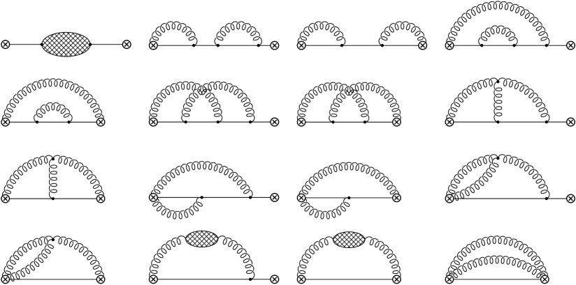
Figure 1: Two-loop diagrams contributing to the jet function in QCD. Gluons emitted from the crossed circles originate from the Wilson lines. Not shown are additional diagrams resulting from mirror images in which the two external points are exchanged. The first diagram is the full fermion two-point function, not just the one-particle irreducible part.

Our calculation of the jet function employs the representation (4) of the function ${\cal J}(p^{2},\mu)$ in terms of ordinary QCD quark and gluon fields. The relevant two-loop diagrams are shown in Figure 1. Equally well, one could use the SCET Lagrangian together with (3) to perform the calculation. In this case diagrams in which a quark emits more than one gluon at the same vertex would also be present, in addition to the topologies shown in Figure 1. Also, the analysis would be complicated by the fact that the SCET Feynman rules are more complicated that those of QCD.

2.1 Evaluation of the two-loop diagrams

We first discuss the evaluation of the bare quantity $j_{\rm bare}(Q^{2})$ and later perform its renormalization. Let us begin by quoting the result for the one-loop master integral

$$\int\!d^{d}k\,\frac{(-1)^{-a-b-c}}{\left(k^{2}+i0\right)^{a}\left[(k+p)^{2}+i0\right]^{b}\left(\bar{n}\cdot k\right)^{c}}=i\pi^{\frac{d}{2}}\left(-p^{2}-i0\right)^{\frac{d}{2}-a-b}\left(\bar{n}\cdot p\right)^{-c}J(a,b,c)\,,$$ (8)

with

$$J(a,b,c)=\frac{\Gamma(\frac{d}{2}-b)\,\Gamma(\frac{d}{2}-a-c)\,\Gamma(a+b-\frac{d}{2})}{\Gamma(a)\,\Gamma(b)\,\Gamma(d-a-b-c)}\,.$$ (9)

At two-loop order, the most general integral we need is (omitting the “$+i0$” terms for brevity)

$$\int\!d^{d}k\,\int\!d^{d}l\, \frac{(-1)^{-a_{1}-a_{2}-a_{3}-b_{1}-b_{2}-b_{3}-c_{1}-c_{2}}}{\left(k^{2}\right)^{a_{1}}\left(l^{2}\right)^{a_{2}}\left[(k-l)^{2}\right]^{a_{3}}\left[(k+p)^{2}\right]^{b_{1}}\left[(l+p)^{2}\right]^{b_{2}}\left[(k+l+p)^{2}\right]^{b_{3}}\left(\bar{n}\cdot k\right)^{c_{1}}\left(\bar{n}\cdot l\right)^{c_{2}}}$$ (10)

$$= -\pi^{d}\left(-p^{2}\right)^{d-a_{1}-a_{2}-a_{3}-b_{1}-b_{2}-b_{3}}\left(\bar{n}\cdot p\right)^{-c_{1}-c_{2}}J(a_{1},a_{2},a_{3},b_{1},b_{2},b_{3},c_{1},c_{2})\,.$$

We use the same standard reduction techniques as in the two-loop calculation of the soft function [2] to express all integrals we need for the evaluation of the diagrams in Figure 1 in terms of four master integrals $M_{n}$. Introducing the dimensional regulator $\epsilon=2-d/2$, we obtain

$$M_{1} = J(1,1,0,0,0,1,0,0)=\frac{\Gamma^{3}(1-\epsilon)\,\Gamma(2\epsilon-1)}{\Gamma(3-3\epsilon)}\,,$$

$$M_{2} = J(1,1,0,1,1,0,0,0)=J(1,1,0)^{2}=\left[\frac{\Gamma^{2}(1-\epsilon)\,\Gamma(\epsilon)}{\Gamma(2-2\epsilon)}\right]^{2},$$

$$M_{3} = J(1,0,1,1,1,0,0,1)=\frac{\Gamma(2\epsilon)}{\epsilon}\int_{0}^{1}\!dx\int_{0}^{1}\!dy\,\frac{(x\bar{x}y^{2}\bar{y})^{-\epsilon}}{1-xy}$$

$$\hskip 100.86496pt=e^{-2\epsilon\gamma_{E}}\left(\frac{\pi^{2}}{12\epsilon^{2}}+\frac{7\zeta_{3}}{2\epsilon}+\frac{11\pi^{4}}{72}+{\cal O}(\epsilon)\right),$$

$$M_{4} = J(1,1,0,1,1,1,1,1)=e^{-2\epsilon\gamma_{E}}\left(\frac{\pi^{2}}{3\epsilon^{2}}-\frac{7\zeta_{3}}{\epsilon}+\frac{23\pi^{4}}{360}+{\cal O}(\epsilon)\right),$$ (11)

where we use the shorthand notation $\bar{x}=1-x$ and $\bar{y}=1-y$. The evaluation of the first three integrals is straightforward. In the case of $M_{3}$ the double parameter integral resulting from the loop integrations can be expanded in $\epsilon$ without difficulty. The calculation of the master integral $M_{4}$, which is needed for the evaluation of the seventh graph in Figure 1, is notably more complicated.

To tackle this last integral we use the Mellin-Barnes technique [14, 15]. The basic strategy is to first introduce Feynman parameters to perform the loop integration and then introduce Mellin-Barnes parameters to carry out the Feynman parameter integrations. What makes this method powerful is that (after analytic continuation to $\epsilon\approx 0$) the Mellin-Barnes integrands can be Taylor expanded about $\epsilon=0$. To start, note that after performing the loop integral over $k$ using conventional Feynman parameters the result for $M_{4}$ can be written as

$$M_{4} = i\pi^{-\frac{d}{2}}\left(-p^{2}\right)^{5-d}\left(\bar{n}\cdot p\right)^{2}\Gamma(3-{\textstyle\frac{d}{2}})\int\!d^{d}l\,\frac{1}{l^{2}\,(l+p)^{2}\,n\cdot l}$$ (12)

$$\times \int_{0}^{1}\!dx\int_{0}^{1}\!dy\,\frac{1}{\bar{n}\cdot p+\bar{y}\,\bar{n}\cdot l}\,\frac{1}{\left(-x^{2}y\bar{y}l^{2}-x\bar{x}\bar{y}(l+p)^{2}-x\bar{x}yp^{2}\right)^{3-\frac{d}{2}}}\,.$$

We now introduce two Mellin-Barnes parameters via

$$(A+B)^{-\alpha}=\frac{1}{2\pi i}\int_{c-i\infty}^{c+i\infty}\!dw\,A^{w}\,B^{-\alpha-w}\,\frac{\Gamma(-w)\,\Gamma(\alpha+w)}{\Gamma(\alpha)}$$ (13)

to break apart the last denominator in (12) into a product with factors $l^{2}$, $(l+p)^{2}$, and $p^{2}$. (We do not introduce a Mellin-Barnes parameter for the denominator $(\bar{n}\cdot p+\bar{y}\,\bar{n}\cdot l)$, as this would lead to ambiguities in the treatment of poles in the resulting light-cone propagators.) We then introduce additional Feynman parameters and perform the loop integration over $l$. We use a third Mellin-Barnes parameter to simplify the resulting Feynman parameter integrals, which can then be expressed in terms of $\Gamma$-functions. This leaves us with the following three-fold Mellin-Barnes integral:

$$M_{4} = \frac{1}{(2\pi i)^{3}}\,\prod_{i=1}^{3}\int_{c_{i}-i\infty}^{c_{i}+i\infty}\!\!dw_{i}\,\frac{\Gamma(-w_{1})\,\Gamma(-w_{2})\,\Gamma(-w_{3})\,\Gamma(1+w_{1})}{\Gamma(-2\epsilon)\,\Gamma(1-2\epsilon+w_{1}+w_{2}+w_{3})\,\Gamma(1-w_{2})\,\Gamma(1-w_{3})}$$ (14)

$$\times \Gamma(-\epsilon-w_{2})\,\Gamma(\epsilon-w_{2}-w_{3})\,\Gamma(1-\epsilon+w_{1}+w_{3})\,\Gamma(1+\epsilon+w_{2}+w_{3})\,\Gamma(1+w_{1}+w_{2}+w_{3})$$

$$\times \Gamma(w_{2}-\epsilon)\,\Gamma(-1-\epsilon-w_{1}-w_{3})\,.$$

In deriving this representation we have interchanged loop, Feynman, and Mellin-Barnes integrations. Careful inspection reveals that the representation (14) is valid if the real parts of all $\Gamma$-functions are positive, i.e., if the poles of each $\Gamma$-function are either all to the left or all to the right of the integration contours. With the choice $c_{1}=-\frac{1}{4}$, $c_{2}=-\frac{1}{8}$, and $c_{3}=-\frac{3}{8}$, this condition is fulfilled if $-\frac{1}{2}<\epsilon<-\frac{3}{8}$. Starting in the allowed range and increasing $\epsilon$, we see that at $\epsilon=-\frac{3}{8}$ the first pole in $\Gamma(-1-\epsilon-w_{1}-w_{3})$ crosses the contour from the right to the left. At $\epsilon=-\frac{1}{8}$ the first pole in $\Gamma(w_{2}-\epsilon)$ crosses from the left to the right. The arguments of all other $\Gamma$-functions remain positive up to $\epsilon<\frac{1}{8}$. To obtain a representation that is valid around $\epsilon=0$, one has to either deform the contours such that the crossings are avoided, or separately take into account the contributions of the poles that end up on the wrong side of the contours as $\epsilon\to 0$, as proposed in [15]. The residues of these poles have again the form of Mellin-Barnes integrals, however with one integration less than the original expression (14). One analyzes these contributions with the same method as the original integral and continues until one ends up with a representation which is valid around $\epsilon=0$. Once this is achieved, the integrands are expanded in $\epsilon$, the integration contours are closed, and the integrations are rewritten as sums over the residues of the poles. In fact, since the original integral includes a factor $1/\Gamma(-2\epsilon)={\cal O}(\epsilon)$, only contributions which arise from poles that cross a contour need to be included in the limit $\epsilon\to 0$. Very recently, the continuation in $\epsilon$ with subsequent numerical evaluation of the integrals has been automatized [16, 17]. We have used the public code of [17] to check our analytical result for $M_{4}$.

As a further independent check of our result we have numerically evaluated the multi-dimensional integral over Feynman parameters, which is obtained after performing the loop integration over $l$ in (12) using conventional methods. As is evident from (2.1) the integral $M_{4}$ is divergent, and the divergences need to be isolated in order to perform the numerical evaluation. We use the method of sector decomposition [18, 19, 20], which allows one to systematically disentangle overlapping singularities in Feynman integrals. This procedure splits the integral into a large number of terms in which all singularities are factorized. Because it leads to large algebraic expressions, the sector decomposition is performed using computer algebra. After numerical integration of the resulting expressions we reproduce the analytical result for the integral $M_{4}$ with a numerical precision of better than 1 part in $10^{6}$.

With the integrals at hand, the evaluation of the two-loop diagrams in Figure 1 is straightforward. We write each diagram as a sum of integrals of the form (10) and express those in terms of the four master integrals $M_{1},\dots,M_{4}$. Summing up the results for the individual diagrams, we obtain

$$j_{\rm bare}(Q^{2}) = 1+\frac{Z_{\alpha}\alpha_{s}}{4\pi}\left(\frac{Q^{2}}{\mu^{2}}\right)^{-\epsilon}C_{F}\left[\frac{4}{\epsilon^{2}}+\frac{3}{\epsilon}+7-\pi^{2}+\left(14-\frac{3\pi^{2}}{4}-\frac{28}{3}\,\zeta_{3}\right)\epsilon\right.$$ (15)

$$\left.\hskip 102.43008pt\mbox{}+\left(28-\frac{7\pi^{2}}{4}-\frac{\pi^{4}}{24}-7\zeta_{3}\right)\epsilon^{2}+{\cal O}(\epsilon^{3})\right]$$

$$\mbox{}+\left(\frac{Z_{\alpha}\alpha_{s}}{4\pi}\right)^{2}\left(\frac{Q^{2}}{\mu^{2}}\right)^{-2\epsilon}C_{F}\,\Big{[}C_{F}K_{F}(\epsilon)+C_{A}K_{A}(\epsilon)+T_{F}n_{f}K_{f}(\epsilon)\Big{]}+\dots\,,$$

where

$$Z_{\alpha}=1-\beta_{0}\,\frac{\alpha_{s}}{4\pi\epsilon}+\dots=1-\left(\frac{11}{3}\,C_{A}-\frac{4}{3}\,T_{F}n_{f}\right)\,\frac{\alpha_{s}}{4\pi\epsilon}+\dots\,.$$ (16)

Here $\alpha_{s}\equiv\alpha_{s}(\mu)$ is the renormalized coupling. Note that the bare jet function is scale independent, since the bare coupling $Z_{\alpha}\alpha_{s}\mu^{2\epsilon}$ does not depend on the renormalization scale. The two-loop coefficients are

$$K_{F}(\epsilon) = \frac{8}{\epsilon^{4}}+\frac{12}{\epsilon^{3}}+\left(\frac{65}{2}-\frac{16\pi^{2}}{3}\right)\frac{1}{\epsilon^{2}}+\left(\frac{311}{4}-9\pi^{2}-\frac{124}{3}\,\zeta_{3}\right)\frac{1}{\epsilon}$$

$$\mbox{}+\frac{1437}{8}-\frac{301\pi^{2}}{12}+\frac{113\pi^{4}}{90}-86\zeta_{3}+{\cal O}(\epsilon)\,,$$

$$K_{A}(\epsilon) = \frac{11}{3\epsilon^{3}}+\left(\frac{233}{18}-\frac{\pi^{2}}{3}\right)\frac{1}{\epsilon^{2}}+\left(\frac{4541}{108}-\frac{55\pi^{2}}{18}-20\zeta_{3}\right)\frac{1}{\epsilon}$$

$$\mbox{}+\frac{86393}{648}-\frac{1129\pi^{2}}{108}-\frac{17\pi^{4}}{180}-\frac{514}{9}\,\zeta_{3}+{\cal O}(\epsilon)\,,$$

$$K_{f}(\epsilon) = -\frac{4}{3\epsilon^{3}}-\frac{38}{9\epsilon^{2}}+\left(-\frac{373}{27}+\frac{10\pi^{2}}{9}\right)\frac{1}{\epsilon}-\frac{7081}{162}+\frac{95\pi^{2}}{27}+\frac{128}{9}\,\zeta_{3}+{\cal O}(\epsilon)\,.$$ (17)

We have checked that the divergences of the first diagram in Figure 1 (together with the appropriate one-loop counter term, and accounting for the renormalization of the gauge parameter) reproduce the known result for the two-loop quark wave-function renormalization [21]. A stringent check of the remaining diagrams with gluon emissions from the Wilson lines is that their divergences must cancel against the jet-function renormalization factor, which we will now derive.

2.2 Renormalization of the jet function

The renormalization of the bare jet function proceeds in complete analogy to that of the bare soft function discussed in [2], to which we refer the reader for a more detailed discussion. The procedure is more complicated than in conventional applications of renormalization owing to the presence of Sudakov double logarithms.

We define an operator renormalization factor for the jet function via

$$J({p^{2}},\mu)=\int d{p^{\prime 2}}\,Z({p^{2}},{p^{\prime 2}},\mu)\,J_{\rm bare}({p^{\prime 2}})\,,$$ (18)

where $Z$ absorbs the UV divergences of the bare jet function, such that the renormalized jet function is finite in the limit $\epsilon\to 0$. In the $\overline{\rm MS}$ regularization scheme, we have

$$Z({p^{2}},{p^{\prime 2}},\mu)=\delta({p^{2}}-{p^{\prime 2}})+\sum_{k=1}^{\infty}\,\frac{1}{\epsilon^{k}}\,Z^{(k)}({p^{2}},{p^{\prime 2}},\mu)\,.$$ (19)

The relations

$$\gamma_{\rm jet}=2\alpha_{s}\,\frac{\partial Z^{(1)}}{\partial\alpha_{s}}\,,\qquad 2\alpha_{s}\,\frac{\partial Z^{(n+1)}}{\partial\alpha_{s}}=2\alpha_{s}\,\frac{\partial Z^{(1)}}{\partial\alpha_{s}}\otimes Z^{(n)}+\beta(\alpha_{s})\,\frac{\partial Z^{(n)}}{\partial\alpha_{s}}+\frac{\partial Z^{(n)}}{\partial\ln\mu}\,,$$ (20)

with $n\geq 1$, connect the coefficient of the $1/\epsilon$ pole in the $Z$ factor to the anomalous dimension and moreover imply a set of consistency conditions among the coefficients of the higher pole terms. The symbol $\otimes$ represents a convolution in $p^{2}$. The term $\partial Z^{(n)}/\partial\ln\mu$ arises because the $Z$ factor depends both implicitly (via the renormalized coupling constant) and explicitly (via Sudakov logarithms contained in star distributions) on the renormalization scale [2].

To all orders in perturbation theory the anomalous-dimension kernel of the jet function has the form

$$\gamma_{\rm jet}({p^{2}},{p^{\prime 2}},\mu)=2\Gamma_{\rm cusp}(\alpha_{s})\left(\frac{1}{{p^{2}}-{p^{\prime 2}}}\right)_{\!*}^{\![\mu^{2}]}+2\gamma^{J}(\alpha_{s})\,\delta({p^{2}}-{p^{\prime 2}})\,,$$ (21)

where $\Gamma_{\rm cusp}$ is the cusp anomalous dimension associated with the Sudakov double logarithms, while $\gamma^{J}$ controls the single-logarithmic evolution of the jet function. The definition of the star distribution can be found in [6]. The corresponding integro-differential evolution equation reads

$$\frac{dJ(p^{2},\mu)}{d\ln\mu}=-\left[2\Gamma_{\rm cusp}\,\ln\frac{p^{2}}{\mu^{2}}+2\gamma^{J}\right]J(p^{2},\mu)-2\Gamma_{\rm cusp}\int_{0}^{p^{2}}\!dp^{\prime 2}\,\frac{J({p^{\prime 2}},\mu)-J(p^{2},\mu)}{p^{2}-{p^{\prime 2}}}\,.$$ (22)

We have derived relation (21) by requiring that the $\bar{B}\to X_{s}\gamma$ decay rate be renormalization-group invariant and using the known evolution equations for the soft function [22] and for the hard matching coefficient [8, 23]. Denoting by $Z_{[n]}$ the coefficient of $(\alpha_{s}/4\pi)^{n}$ in $Z({p^{2}},{p^{\prime 2}},\mu)$, we obtain from (20)

$$Z_{[0]} = \delta({p^{2}}-{p^{\prime 2}})\,,$$

$$Z_{[1]} = \delta({p^{2}}-{p^{\prime 2}})\left(-\frac{\Gamma_{0}}{\epsilon^{2}}+\frac{\gamma^{J}_{0}}{\epsilon}\right)+\frac{\Gamma_{0}}{\epsilon}\left(\frac{1}{{p^{2}}-{p^{\prime 2}}}\right)_{\!*}^{\![\mu^{2}]},$$

$$Z_{[2]} = \delta({p^{2}}-{p^{\prime 2}})\left[\frac{\Gamma_{0}^{2}}{2\epsilon^{4}}-\frac{\Gamma_{0}(\gamma^{J}_{0}-\frac{3}{4}\beta_{0})}{\epsilon^{3}}+\left(\frac{\gamma^{J}_{0}(\gamma^{J}_{0}-\beta_{0})}{2}-\frac{\Gamma_{1}}{4}-\frac{\pi^{2}}{12}\,\Gamma_{0}^{2}\right)\frac{1}{\epsilon^{2}}+\frac{\gamma^{J}_{1}}{2\epsilon}\right]$$ (23)

$$\mbox{}+\left[-\frac{\Gamma_{0}^{2}}{\epsilon^{3}}+\frac{\Gamma_{0}(\gamma^{J}_{0}-\frac{1}{2}\beta_{0})}{\epsilon^{2}}+\frac{\Gamma_{1}}{2\epsilon}\right]\left(\frac{1}{{p^{2}}-{p^{\prime 2}}}\right)_{\!*}^{\![\mu^{2}]}+\frac{\Gamma_{0}^{2}}{\epsilon^{2}}\left(\frac{\ln\frac{{p^{2}}-{p^{\prime 2}}}{\mu^{2}}}{{p^{2}}-{p^{\prime 2}}}\right)_{\!*}^{\![\mu^{2}]},$$

where the expansion coefficients of the anomalous dimensions and $\beta$-function are defined as

$$\Gamma_{\rm cusp}(\alpha_{s}) = \sum_{n=0}^{\infty}\,\Gamma_{n}\left(\frac{\alpha_{s}}{4\pi}\right)^{n+1},\qquad\gamma^{J}(\alpha_{s})=\sum_{n=0}^{\infty}\,\gamma_{n}\left(\frac{\alpha_{s}}{4\pi}\right)^{n+1},$$

$$\beta(\alpha_{s}) = \frac{d\alpha_{s}}{d\ln\mu}=-2\alpha_{s}\sum_{n=0}^{\infty}\,\beta_{n}\left(\frac{\alpha_{s}}{4\pi}\right)^{n+1}.$$ (24)

The expression for the two-loop cusp anomalous dimension can be found, e.g., in our previous paper [2]. The two-loop anomalous dimension of the jet function has never been calculated directly, but it was inferred in [1] from existing two-loop results for jet-function moments in deep-inelastic scattering [24]. In that way one obtains

$$\gamma_{0}^{J} = -3C_{F}\,,$$ (25)

$$\gamma_{1}^{J} = C_{F}^{2}\left(-\frac{3}{2}+2\pi^{2}-24\zeta_{3}\right)+C_{F}C_{A}\left(-\frac{1769}{54}-\frac{11\pi^{2}}{9}+40\zeta_{3}\right)+C_{F}T_{F}n_{f}\left(\frac{242}{27}+\frac{4\pi^{2}}{9}\right)\,.$$

It is straightforward to show that the function $j(\ln\frac{Q^{2}}{\mu^{2}},\mu)$ obeys the same evolution equation as the original jet function $J(p^{2},\mu)$, i.e.

$$j\Big{(}\ln\frac{Q^{2}}{\mu^{2}},\mu\Big{)}=\int_{0}^{Q^{2}}\!dQ^{\prime 2}\,Z(Q^{2},Q^{\prime 2},\mu)\,j_{\rm bare}(Q^{\prime 2})\,,$$ (26)

where $j_{\rm bare}(Q^{2})$ is the quantity we have calculated in Section 2.1. Expanding this relation in perturbation theory we obtain $j_{[0]}=j_{[0]}^{\rm bare}=1$ and

$$j_{[1]}=j_{[1]}^{\rm bare}+Z_{[1]}\otimes j_{[0]}^{\rm bare}\,,\qquad j_{[2]}=j_{[2]}^{\rm bare}+Z_{[1]}\otimes j_{[1]}^{\rm bare}+Z_{[2]}\otimes j_{[0]}^{\rm bare}\,.$$ (27)

The first term on the right-hand side in each equation corresponds to the contribution (15) obtained from the loop diagrams. The remaining terms correspond to the counter-term contributions. Explicitly, we find

$$j_{[1]}^{\rm C.T.} = -\frac{\Gamma_{0}}{\epsilon^{2}}+\frac{\gamma^{J}_{0}}{\epsilon}+\frac{\Gamma_{0}}{\epsilon}\,\ln\frac{Q^{2}}{\mu^{2}}\,,$$

$$j_{[2]}^{\rm C.T.} = \left[-\frac{\Gamma_{0}}{\epsilon^{2}}+\frac{\gamma^{J}_{0}}{\epsilon}+\frac{\Gamma_{0}}{\epsilon}\left(\ln\frac{Q^{2}}{\mu^{2}}-\gamma_{E}-\psi(1-\epsilon)\right)\right]j_{[1]}^{\rm bare}(Q^{2})$$ (28)

$$\mbox{}+\frac{\Gamma_{0}^{2}}{2\epsilon^{4}}-\frac{\Gamma_{0}(\gamma^{J}_{0}-\frac{3}{4}\beta_{0})}{\epsilon^{3}}+\left(\frac{\gamma^{J}_{0}(\gamma^{J}_{0}-\beta_{0})}{2}-\frac{\Gamma_{1}}{4}-\frac{\pi^{2}}{12}\,\Gamma_{0}^{2}\right)\frac{1}{\epsilon^{2}}+\frac{\gamma^{J}_{1}}{2\epsilon}$$

$$\mbox{}+\left[-\frac{\Gamma_{0}^{2}}{\epsilon^{3}}+\frac{\Gamma_{0}(\gamma^{J}_{0}-\frac{1}{2}\beta_{0})}{\epsilon^{2}}+\frac{\Gamma_{1}}{2\epsilon}\right]\ln\frac{Q^{2}}{\mu^{2}}+\frac{\Gamma_{0}^{2}}{2\epsilon^{2}}\,\ln^{2}\frac{Q^{2}}{\mu^{2}}\,.$$

Together with the results for the bare one-loop jet function from (15) this yields explicit expressions for the counter terms. When adding these contributions to the bare jet function we find that all $1/\epsilon^{n}$ pole terms cancel, so that the limit $\epsilon\to 0$ can now be taken. This implies, in particular, that we confirm by direct calculation the expression for the anomalous-dimension coefficient $\gamma_{1}^{J}$ given in (25).

2.3 Results

The logarithmic terms in the renormalized jet function have been determined in [3] by solving the renormalization-group equation perturbatively. At two-loop order, it was found that

$$j(L,\mu) = 1+\frac{\alpha_{s}(\mu)}{4\pi}\left[b_{0}^{(1)}+\gamma_{0}^{J}L+\frac{\Gamma_{0}}{2}\,L^{2}\right]$$ (29)

$$\mbox{}+\left(\frac{\alpha_{s}(\mu)}{4\pi}\right)^{2}\Bigg{[}b_{0}^{(2)}+\left(b_{0}^{(1)}(\gamma_{0}^{J}-\beta_{0})+\gamma_{1}^{J}-\frac{\pi^{2}}{6}\,\Gamma_{0}\gamma_{0}^{J}+\zeta_{3}\,\Gamma_{0}^{2}\right)L$$

$$\quad\mbox{}+\frac{1}{2}\left(\gamma_{0}^{J}(\gamma_{0}^{J}-\beta_{0})+b_{0}^{(1)}\,\Gamma_{0}+\Gamma_{1}-\frac{\pi^{2}}{6}\,\Gamma_{0}^{2}\right)L^{2}+\frac{\Gamma_{0}}{2}\left(\gamma_{0}^{J}-\frac{\beta_{0}}{3}\right)L^{3}+\frac{\Gamma_{0}^{2}}{8}\,L^{4}\Bigg{]}\,.\qquad$$

Our results for the logarithmic terms agree with the above expression. The one-loop coefficient $b_{0}^{(1)}$ was derived in [5, 6]. The main new result is $b_{0}^{(2)}$, the constant term at two-loop order. We obtain

$$b_{0}^{(1)} = (7-\pi^{2})\,C_{F}\,,$$

$$b_{0}^{(2)} = C_{F}^{2}\left(\frac{205}{8}-\frac{67\pi^{2}}{6}+\frac{14\pi^{4}}{15}-18\zeta_{3}\right)+C_{F}C_{A}\left(\frac{53129}{648}-\frac{208\pi^{2}}{27}-\frac{17\pi^{4}}{180}-\frac{206}{9}\,\zeta_{3}\right)$$ (30)

$$\mbox{}+C_{F}T_{F}n_{f}\left(-\frac{4057}{162}+\frac{68\pi^{2}}{27}+\frac{16}{9}\,\zeta_{3}\right).$$

It is interesting to compare the exact answer for the coefficient $b_{0}^{(2)}$ with the approximation obtained by keeping only the terms of order $\beta_{0}\alpha_{s}^{2}$. In the absence of exact two-loop results it is sometimes argued that the $\beta_{0}\alpha_{s}^{2}$ terms constitute the dominant part of the complete two-loop correction. In the present case, we obtain for $N_{c}=3$ colors $b_{0}^{(2)}\approx-16.25x-128.78\approx-145.04$, where $x=\frac{3}{25}\,\beta_{0}=1$ for $n_{f}=4$ light flavors. Keeping only the $\beta_{0}\alpha_{s}^{2}$ terms would give $-16.25$, which is off by an order of magnitude. This illustrates the importance of performing exact two-loop calculations.

We now briefly discuss the impact of our results for phenomenology. Besides the jet function $j(L,\mu)$ itself, it is useful to consider a related function $\widetilde{j}(L,\mu)$ obtained by replacing the $n$-th power of $L$ in (2) with an $n$-th order polynomial, $L^{n}\to I_{n}(L)$, where at two-loop order we need

$$I_{1}(x) = x\,,\hskip 56.9055ptI_{3}(x)=x^{3}+\frac{\pi^{2}}{2}\,x-2\zeta_{3}\,,$$

$$I_{2}(x) = x^{2}+\frac{\pi^{2}}{6}\,,\qquad I_{4}(x)=x^{4}+\pi^{2}x^{2}-8\zeta_{3}\,x+\frac{3\pi^{4}}{20}\,.$$ (31)

The function $\widetilde{j}$ enters in the factorization formula for the partial $\bar{B}\to X_{s}\gamma$ decay rate with a cut on photon energy [3]. For the case of $N_{c}=3$ colors and $n_{f}=4$ light quark flavors we get

$$j(L,\mu) \approx 1+\left(-0.304-0.318L+0.212L^{2}\right)\alpha_{s}(\mu)$$

$$\mbox{}+\left(-0.918+0.926L+0.079L^{2}-0.114L^{3}+0.023L^{4}\right)\alpha_{s}^{2}(\mu)+\dots\,,$$

$$\widetilde{j}(L,\mu) \approx 1+\left(0.045-0.318L+0.212L^{2}\right)\alpha_{s}(\mu)$$ (32)

$$\mbox{}+\left(-0.185+0.145L+0.301L^{2}-0.114L^{3}+0.023L^{4}\right)\alpha_{s}^{2}(\mu)+\dots\,.$$

The two-loop corrections to $j$ are very large and, for realistic parameter values, can even dominate over the one-loop corrections. However, the two-loop corrections are much smaller for the function $\widetilde{j}$. Figure 2 shows the dependence of the two jet functions on $L=\ln(Q^{2}/\mu^{2})$ for a fixed scale $\mu\approx 2$ GeV chosen such that $\alpha_{s}(\mu)=0.3$, corresponding to a renormalization point appropriate for the calculation of the partial $\bar{B}\to X_{s}\gamma$ decay rate with a cut $E_{\gamma}>1.8$ GeV. The two-loop effects calculated in this work impact the jet function $j$ at the 10% level, while their effect on the function $\widetilde{j}$ is at the level of 2% or less. The latter finding suggests a good convergence of the perturbative expansion at the intermediate scale in the analysis of $\bar{B}\to X_{s}\gamma$ decay. In addition to the one- and two-loop predictions, the figure also displays the results obtained if only terms of order $\beta_{0}\alpha_{s}^{2}$ are kept in the two-loop coefficients. In both cases this provides a poor approximation to the exact two-loop results. We also note that the jet functions by themselves are not renormalization-group invariant, so it is meaningless to study their dependence on the scale $\mu$ for fixed $Q^{2}$. In physical results such as the expression for the $\bar{B}\to X_{s}\gamma$ decay rate and photon-energy moments given in [1, 3], the scale dependence of the jet function cancels against that of other renormalization-group functions.

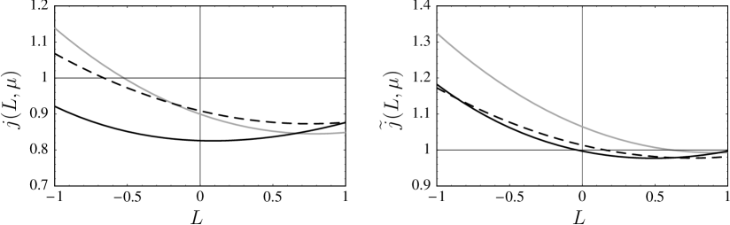
Figure 2: One- and two-loop predictions for the jet functions $j(L,\mu)$ and $\widetilde{j}(L,\mu)$ evaluated at $\alpha_{s}(\mu)=0.3$. The dashed lines show the one-loop results, while the solid lines give the complete two-loop results derived in the present work. The gray lines are obtained if only the $\beta_{0}\alpha_{s}^{2}$ terms are kept in the two-loop contributions.

3 Moments of the jet function

In the analysis of hard QCD processes such as deep-inelastic scattering it is often convenient to introduce moments of the jet function defined as (see e.g. [25])

$$J_{N}(Q^{2},\mu)=\int_{0}^{Q^{2}}\!dp^{2}\left(1-\frac{p^{2}}{Q^{2}}\right)^{N-1}J(p^{2},\mu)\,.$$ (33)

Whereas in inclusive $B$ decays the scale $Q^{2}$ setting the upper integration limit in (1) is an intermediate (hard-collinear) scale, $Q^{2}\ll m_{b}^{2}$, which is of order the invariant mass squared of the final-state hadronic jet, the variable $Q^{2}$ in (33) is set by a characteristic hard scale of the process. In the large-$N$ limit the integral receives leading contributions only from the region $p^{2}\sim Q^{2}/N\ll Q^{2}$. The scale $Q^{2}/N$ is the analog of the intermediate scale in $\bar{B}\to X_{s}\gamma$ decay.

Using an integration by parts, it is straightforward to express the jet-function moments in terms of integrals over the function $j$ calculated at two-loop order in the present work. We obtain

$$J_{1}(Q^{2},\mu)=j\Big{(}\ln\frac{Q^{2}}{\mu^{2}},\mu\Big{)}\,,\qquad J_{N}(Q^{2},\mu)=(N-1)\int_{0}^{1}\!dx\,(1-x)^{N-2}\,j\Big{(}\ln\frac{xQ^{2}}{\mu^{2}},\mu\Big{)}\,,$$ (34)

where the second relation holds for $N\geq 2$. It follows from (22) that the moments obey the evolution equation

$$\frac{dJ_{N}(Q^{2},\mu)}{d\ln\mu} = -\left[2\Gamma_{\rm cusp}\left(\ln\frac{Q^{2}}{\mu^{2}}-H_{N-1}\right)+2\gamma^{J}\right]J_{N}(Q^{2},\mu)$$ (35)

$$\mbox{}-2\Gamma_{\rm cusp}\int_{0}^{Q^{2}}\!dp^{2}\left(1-\frac{p^{2}}{Q^{2}}\right)^{N-1}\ln\left(1-\frac{p^{2}}{Q^{2}}\right)J(p^{2},\mu)\,,$$

where $H_{N-1}=\sum_{n=1}^{N-1}\frac{1}{n}$ is the harmonic number. These results simplify greatly in the large-$N$ limit. We find that the moments are given by

$$J_{N}(Q^{2},\mu)=\widetilde{j}\Big{(}\ln\frac{Q^{2}}{e^{\gamma_{E}}N\mu^{2}},\mu\Big{)}+{\cal O}\left(\frac{1}{N}\right),$$ (36)

and that they obey the local evolution equation

$$\frac{dJ_{N}(Q^{2},\mu)}{d\ln\mu}=-\left[2\Gamma_{\rm cusp}\,\ln\frac{Q^{2}}{e^{\gamma_{E}}N\mu^{2}}+2\gamma^{J}\right]J_{N}(Q^{2},\mu)+{\cal O}\left(\frac{1}{N}\right).$$ (37)

In deriving this result we have used that the second line in (35) is suppressed in the large-$N$ limit, since $p^{2}/Q^{2}={\cal O}(1/N)$ in the argument of the logarithm. This local evolution equation can be integrated using standard techniques.

4 Conclusions

We have calculated the two-loop expression for the jet function $j(L,\mu)$ defined in terms of an integral over the hard-collinear quark propagator in soft-collinear effective theory. This quantity is a necessary ingredient for the NNLO evaluation of the $\bar{B}\to X_{s}\gamma$ decay rate with a cut on the photon energy. Moreover, since the jet function is universal, it appears in many other applications of perturbative QCD. The results obtained in the present work, when combined with [2], provide a complete description of low-scale effects in the analysis of the partial $\bar{B}\to X_{s}\gamma$ decay rate at NNLO in renormalization-group improved perturbation theory. A detailed study of the phenomenological impact of these effects will be presented elsewhere.

Acknowledgments

We thank Frank Petriello for discussions and for numerically evaluating the master integral $M_{4}$. The research of T.B. was supported by the Department of Energy under Grant DE-AC02-76CH03000. The research of M.N. was supported by the National Science Foundation under Grant PHY-0355005. Fermilab is operated by Universities Research Association Inc., under contract with the U.S. Department of Energy.

References

[1]
M. Neubert,
Eur. Phys. J. C 40, 165 (2005)
[hep-ph/0408179].
[2]
T. Becher and M. Neubert,
Phys. Lett. B 633, 739 (2006)
[hep-ph/0512208].
[3]
M. Neubert,
Phys. Rev. D 72, 074025 (2005)
[hep-ph/0506245].
[4]
G. Sterman,
Nucl. Phys. B 281, 310 (1987).
[5]
C. W. Bauer and A. V. Manohar,
Phys. Rev. D 70, 034024 (2004)
[hep-ph/0312109].
[6]
S. W. Bosch, B. O. Lange, M. Neubert and G. Paz,
Nucl. Phys. B 699, 335 (2004)
[hep-ph/0402094].
[7]
F. De Fazio and M. Neubert,
JHEP 9906, 017 (1999)
[hep-ph/9905351].
[8]
C. W. Bauer, S. Fleming, D. Pirjol and I. W. Stewart,
Phys. Rev. D 63, 114020 (2001)
[hep-ph/0011336].
[9]
C. W. Bauer, D. Pirjol and I. W. Stewart,
Phys. Rev. D 65, 054022 (2002)
[hep-ph/0109045].
[10]
M. Beneke, A. P. Chapovsky, M. Diehl and T. Feldmann,
Nucl. Phys. B 643, 431 (2002)
[hep-ph/0206152].
[11]
R. J. Hill and M. Neubert,
Nucl. Phys. B 657, 229 (2003)
[hep-ph/0211018].
[12]
M. Beneke and T. Feldmann,
Phys. Lett. B 553, 267 (2003)
[hep-ph/0211358].
[13]
T. Becher, R. J. Hill and M. Neubert,
Phys. Rev. D 69, 054017 (2004)
[hep-ph/0308122].
[14]
V. A. Smirnov,
Phys. Lett. B 460, 397 (1999)
[hep-ph/9905323].
[15]
J. B. Tausk,
Phys. Lett. B 469, 225 (1999)
[hep-ph/9909506].
[16]
C. Anastasiou and A. Daleo,
hep-ph/0511176.
[17]
M. Czakon,
hep-ph/0511200.
[18]
K. Hepp,
Commun. Math. Phys. 2, 301 (1966).
[19]
T. Binoth and G. Heinrich,
Nucl. Phys. B 585, 741 (2000)
[hep-ph/0004013].
[20]
C. Anastasiou, K. Melnikov and F. Petriello,
Phys. Rev. D 69, 076010 (2004)
[hep-ph/0311311].
[21]
E. Egorian and O. V. Tarasov,
Theor. Math. Phys. 41, 863 (1979)
[Teor. Mat. Fiz. 41, 26 (1979)].
[22]
A. G. Grozin and G. P. Korchemsky,
Phys. Rev. D 53, 1378 (1996)
[hep-ph/9411323].
[23]
T. Becher, R. J. Hill, B. O. Lange and M. Neubert,
Phys. Rev. D 69, 034013 (2004)
[hep-ph/0309227].
[24]
A. Vogt,
Phys. Lett. B 497, 228 (2001)
[hep-ph/0010146].
[25]
S. Catani, B. R. Webber and G. Marchesini,
Nucl. Phys. B 349, 635 (1991).