$e^{+}e^{-}$ angularity distributions at NNLL^′ accuracy

Abstract

We present predictions for the $e^{+}e^{-}$ event shape angularities at NNLL^′ resummed and $\mathcal{O}(\alpha_{s}^{2})$ matched accuracy and compare them to LEP data at center-of-mass energies $Q=91.2$ GeV and $Q=197$ GeV. We perform the resummation within the framework of Soft-Collinear Effective Theory, and make use of recent results for the two-loop angularity soft function. We determine the remaining NNLL^′ and $\mathcal{O}(\alpha_{s}^{2})$ ingredients from a fit to the EVENT2 generator, and implement a shape function with a renormalon-free gap parameter to model non-perturbative effects. Using values of the strong coupling $\alpha_{s}(m_{Z})$ and the universal non-perturbative shift parameter $\Omega_{1}$ that are consistent with those obtained in previous fits to the thrust and $C$-parameter distributions, we find excellent agreement between our predictions and the LEP data for all angularities with $a\in[-1,0.5]$. This provides a robust test of the predictions of QCD, factorization, and the universal scaling of the non-perturbative shift across different angularities. Promisingly, our results indicate that current degeneracies in the $\{\alpha_{s}(m_{Z}),\Omega_{1}\}$ parameter space could be alleviated upon fitting these parameters to experimental data for the angularity distributions.

LA-UR-18-24071

DESY 18-083

SI-HEP-2018-19

1 Introduction

Event-shape variables are classic QCD observables that characterize the geometric properties of a hadronic final-state distribution in high-energy collisions Dasgupta:2003iq . They have been measured to high accuracy at LEP and other $e^{+}e^{-}$ colliders in the past, and are commonly used for determinations of the strong coupling constant $\alpha_{s}$. Whereas past $\alpha_{s}$ extractions from event shapes were often limited by perturbative uncertainties, various theoretical developments triggered a renewed interest in event-shape data in the past decade.

The theoretical description of event-shape distributions combines elements from QCD in different regimes. For generic values of the event shape, the distributions can be described in fixed-order perturbation theory where, currently, $\mathcal{O}(\alpha_{s}^{3})$ corrections are known for a large class of variables GehrmannDeRidder:2007hr ; Weinzierl:2009ms ; Ridder:2014wza ; DelDuca:2016ily . In phase-space regions in which the QCD radiation is confined to jet-like configurations, the perturbative expansion develops large logarithmic corrections that need to be controlled to all orders. The resummation of these Sudakov logarithms was pioneered in Catani:1992ua using the coherent branching formalism, and has since been reformulated and pushed to new levels of accuracy with methods from Soft-Collinear Effective Theory (SCET) Bauer:2000ew ; Bauer:2000yr ; Bauer:2001yt ; Beneke:2002ph . To date, resummations for a variety of event-shape variables have been worked out to impressively high accuracies, e.g. to next-to-next-to-leading logarithmic (NNLL) deFlorian:2004mp ; Becher:2012qc ; Banfi:2014sua and even N³LL order Becher:2008cf ; Chien:2010kc ; Hoang:2014wka .

The resummation of the logarithmic corrections tames the singular behaviour of the cross section near the kinematic endpoint and generates a characteristic peak structure whose shape is affected by non-perturbative physics. For the tails of the distributions—the region commonly used for the $\alpha_{s}$ determinations—the non-perturbative effects typically result in a shift of the perturbative distribution that is driven by a non-perturbative but universal parameter $\Omega_{1}$. Current $\alpha_{s}$ extractions from event shapes (see e.g. Davison:2008vx ; Abbate:2010xh ; Abbate:2012jh ; Gehrmann:2012sc ; Hoang:2015hka ) are therefore organized as two-dimensional $\{\alpha_{s}(m_{Z}),\Omega_{1}\}$ fits to the experimental data. The parameter $\Omega_{1}$ is universal in the sense that the leading non-perturbative shift to a large number of event shapes depends only on this single parameter, scaled by exactly calculable observable-dependent coefficients, as can be demonstrated using factorization and an operator product expansion Lee:2006fn ; Lee:2006nr ; Becher:2013iya . This universality does, however, require a careful consideration of hadron mass effects Salam:2001bd ; Mateu:2012nk . It is therefore possible to reduce the correlation between $\alpha_{s}(m_{Z})$ and $\Omega_{1}$ in the two-dimensional fits by including data from different event-shape variables.

The most precise $\alpha_{s}$ extractions from event shapes to date are based on the thrust Abbate:2010xh ; Abbate:2012jh and $C$-parameter Hoang:2015hka variables. In these works the authors combine an N³LL resummation of large logarithmic corrections in the two-jet region together with fixed-order predictions up to $\mathcal{O}(\alpha_{s}^{3})$ accuracy in the multi-jet region, and they use a shape function that reproduces the aforementioned shift in the tail region to model non-perturbative effects. While the values of $\alpha_{s}(m_{Z})$ the authors find from these fits are very precise and consistent with each other, they are noticeably below the world average PhysRevD.98.030001 (see also Bethke:2011tr ). As can be seen, e.g., in Fig. 4 of Hoang:2015hka , the low value of $\alpha_{s}(m_{Z})$ seems to be associated with the implementation of non-perturbative effects. It is therefore important to test the underlying assumptions of the non-perturbative physics with other event-shape variables.

In the present work we analyze a class of event shapes known as angularities, which are defined as Berger:2003iw

$$\tau_{a}=\frac{1}{Q}\,\underset{i}{\sum}\;|{\bf p}_{\perp}^{i}|\;e^{-|\eta_{i}|(1-a)}\,,$$ (1)

where $Q$ is the center-of-mass energy of the collision and the sum runs over all final-state particles $i$ with rapidity $\eta_{i}$ and transverse momentum ${\bf p}_{\perp}^{i}$ with respect to the thrust axis. The angularities depend on a continuous parameter $a$, and they include thrust ($a=0$) and total jet broadening ($a=1$) as special cases. Whereas infrared safety requires that $a<2$, we restrict our attention to values of $a\leq 0.5$ in this work, since soft recoil effects which complicate the resummation are known to become increasingly more important as $a\to 1$ Dokshitzer:1998kz . It is also possible to define $\tau_{a}$ in Eq. (1) with respect to an axis other than the thrust axis, such as the broadening axis or another soft-recoil-insensitive axis Larkoski:2014uqa . We stick to the standard thrust-axis-based definition here, to coincide with the available data. See Procura:2018zpn for a recent calculation with an alternative axis.

The phenomenological effect of varying $a$ is to change the proportions of two-jet-like events and three-or-more-jet-like events that populate the peak region of the $\tau_{a}$ distributions (see Fig. 1). The relevant collinear scale that enters the factorization of angularity distributions in the two-jet limit then varies accordingly with $a$, to properly reflect the transverse size of the jets that are dominating each region of the distributions.

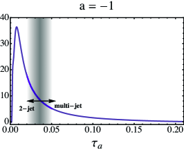
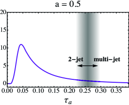
Figure 1: Angularity distributions at NNLL${}^{\prime}+\mathcal{O}(\alpha_{s}^{2})$ accuracy, convolved with a renormalon-free non-perturbative shape function, whose calculation is the subject of this paper. We display the predictions for three values of $a$ (for now without uncertainties), illustrating roughly where two-jet and three-or-more-jet events lie in each $\tau_{a}$ spectrum. For this illustration, the boundary is drawn at the value of $\tau_{a}$ for a four-particle state that is grouped into pairs of jets with opening angle $30^{\circ}$. As $a$ becomes larger (smaller), the peak region is more (less) dominated by purely two-jet events.

The resummation of Sudakov logarithms for the angularity distributions is based on the factorization theorem Berger:2003iw ; Bauer:2008dt ; Hornig:2009vb ; Almeida:2014uva

$$\frac{1}{\sigma_{0}}\frac{d\sigma}{d\tau_{a}}(\tau_{a})=H(Q^{2},\mu)\int dt_{n}^{a}\,dt_{\bar{n}}^{a}\,dk_{s}\,J_{n}^{a}(t_{n}^{a},\mu)\,J_{\bar{n}}^{a}(t_{\bar{n}}^{a},\mu)\,S^{a}(k_{s},\mu)\;\delta\Bigl{(}\tau_{a}-\frac{t_{n}^{a}+t_{\bar{n}}^{a}}{Q^{2-a}}-\frac{k_{s}}{Q}\Bigr{)}\,,$$ (2)

which arises in the two-jet limit $\tau_{a}\to 0$. Here $H$ is a hard function that contains the virtual corrections to $e^{+}e^{-}\to q\bar{q}$ scattering at center-of-mass energy $Q$ (normalised to the Born cross section $\sigma_{0}$); $J_{n,{\bar{n}}}^{a}$ are quark jet functions that describe the collinear emissions into the jet directions, and are functions of a variable $t_{n,{\bar{n}}}^{a}$ of mass dimension $(2-a)$; and $S^{a}$ is a soft function that encodes the low-energetic cross talk between the two jets and depends on a variable $k_{s}$ of mass dimension $1$. In the language of SCET, the angularities are of SCET_I type, since the virtuality of the soft modes $\mu_{S}^{2}\sim Q^{2}\tau_{a}^{2}$ is smaller than that of the collinear modes $\mu_{J}^{2}\sim Q^{2}\tau_{a}^{2/(2-a)}$ for $a<1$. In contrast, jet broadening with $a=1$ corresponds to a SCET_II observable, which requires somewhat different techniques for the resummation of the logarithmic corrections Becher:2011pf ; Chiu:2012ir .

For very small values of $\tau_{a}$, the soft scale becomes non-perturbative and the soft effects are often parametrized by a non-perturbative shape function that is convolved with the perturbative distribution Korchemsky:1998ev ; Korchemsky:1999kt . The dominant effect of the shape function in the tail region is a shift of the perturbative distribution:

$$\frac{d\sigma}{d\tau_{a}}(\tau_{a})\underset{\text{NP}}{\longrightarrow}\frac{d\sigma}{d\tau_{a}}\Big{(}\tau_{a}-c_{\tau_{a}}\frac{\Omega_{1}}{Q}\Big{)}\,.$$ (3)

This form of the shift, scaling as $1/Q$ and with a value of $c_{\tau_{a}}=2/(1-a)$ for the angularity-dependent coefficient, was argued for in Berger:2003pk ; Berger:2004xf based on the infrared behavior of the resummed perturbative exponent Korchemsky:1999kt and on dressed gluon exponentation Gardi:2001di , building upon earlier models of an effective infrared coupling leading to the proposed universal form of the shift in Eq. (3) for numerous event shapes Dokshitzer:1995qm ; Dokshitzer:1995zt ; Dokshitzer:1998pt . This universal form was later proven to all orders in soft emissions by an operator analysis in Lee:2006nr . In the latter work, a definition of the non-perturbative parameter $\Omega_{1}$ was obtained as a vacuum matrix element of soft Wilson lines and a transverse energy-flow operator. More importantly, it turns out that $\Omega_{1}$ is the same non-perturbative parameter that enters the thrust analysis, related through the coefficient $c_{\tau_{a}}$. The growth of the shift with larger $a$ reflects the greater dominance of narrow two-jet events in the peaks of the $\tau_{a}$ distributions than for smaller $a$ (see Fig. 1). It is one of the purposes of this work to provide a state-of-the-art description of the angularity distributions in order to verify if the angularity-dependent shift is reflected in the experimental data.

To this end we will significantly improve the theoretical description of the angularity distributions for which, up until this year, the NLL^′+$\mathcal{O}(\alpha_{s})$ calculation from Hornig:2009vb represented the highest accuracy achieved. However, a recent calculation of the two-loop angularity soft function Bell:2015lsf ; Bell:2018vaa ; Bell:2018oqa allows the distributions to immediately be extended to NNLL accuracy, and indeed NNLL predictions using these two-loop results appeared recently in Procura:2018zpn in the context of multi-differential observables. NNLL predictions were also obtained using the ARES formalism in Banfi:2018mcq . In this paper, we will further extend these results to NNLL${}^{\prime}+\mathcal{O}(\alpha_{s}^{2})$ accuracy by utilizing the EVENT2 generator to determine the missing singular ingredients (the constant in the two-loop angularity jet function) and the full non-singular part of the fixed-order $\mathcal{O}(\alpha_{s}^{2})$ prediction. Furthermore, in order to treat non-perturbative effects, we convolve the improved perturbative distribution with a shape function,

$$\frac{1}{\sigma_{0}}\,\sigma(\tau_{a})=\int dk\,\sigma_{\text{PT}}\Bigl{(}\tau_{a}-\frac{k}{Q};\mu_{H},\mu_{J},\mu_{S},\mu_{\text{ns}}\Bigr{)}\Bigl{[}e^{-2\delta_{a}(\mu_{S},R)\frac{d}{dk}}f_{\text{mod}}\bigl{(}k-2\Delta_{a}(\mu_{S},R)\bigr{)}\Bigr{]}\,,$$ (4)

where $\sigma_{\text{PT}}$ represents the perturbative prediction. In our notation, $\sigma$ and $\sigma_{\text{PT}}$ can represent either the differential or integrated spectra,

$$\sigma=\frac{d\sigma}{d\tau_{a}}\qquad\text{or}\qquad\sigma=\sigma_{c}\equiv\int^{\tau_{a}}d\tau_{a}^{\prime}\,\frac{d\sigma}{d\tau_{a}^{\prime}}\,.$$ (5)

The perturbative cross section $\sigma_{\text{PT}}$ depends on the scales $\mu_{H,J,S}$ associated with the factorization into hard, jet, and soft functions in the two-jet region (see Eq. (2)), and a scale $\mu_{\text{ns}}$ related to nonsingular terms in $\tau_{a}$ which are predicted in fixed-order perturbation theory, but which are not contained in the factorized part of $\sigma_{\text{PT}}$. That is, one can write the perturbative distribution as

$$\sigma_{\text{PT}}(\tau_{a};\mu_{H},\mu_{J},\mu_{S},\mu_{\text{ns}})=\sigma_{\text{sing}}(\tau_{a};\mu_{H},\mu_{J},\mu_{S})+\sigma_{\text{ns}}(\tau_{a},\mu_{\text{ns}})\,.$$ (6)

The non-perturbative shape function $f_{\text{mod}}$ contains a gap parameter $\Delta_{a}$ accounting for the minimum value of $\tau_{a}$ for a hadronic (as opposed to partonic) spectrum, while $R$ is the scale of subtraction terms $\delta_{a}(\mu_{S},R)$ that remove renormalon ambiguities between $\Delta_{a}$ and the perturbative soft function Hoang:2007vb . Formal definitions of all these objects will be given below.

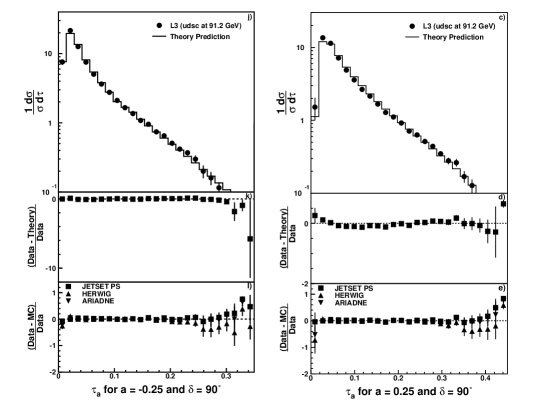
Figure 2: Sample data at $Q=91.2$ GeV from the L3 collaboration Achard:2011zz for two angularities: $a=-0.25$ and $a=0.25$. The theory predictions in the top panels are based on Berger:2003pk ; Berger:2003zh ; Berger:2004xf , which include the prediction of the non-perturbative scaling rule in Eq. (3).

Finally, we compare our predictions to experimental data from the L3 Collaboration Achard:2011zz , which provides measurements of the angularity distributions for eight different values of $a\in\{-1.0,\,-0.75,\,-0.5,\,-0.25,\,0.0,\,0.25,\,0.5,\,0.75\}$ at center-of-mass energies $Q=91.2$ GeV and $Q=197$ GeV (though we will stick to seven values in our analysis, leaving out $a=0.75$ due to uncontrolled $a\to 1$ corrections). The $Q=91.2$ GeV data for two values of $a$ is shown in Fig. 2 for illustration. The L3 analysis also includes a comparison of this data with different Monte-Carlo event generators and NLL theory predictions from Berger:2003pk ; Berger:2003zh ; Berger:2004xf , which include the non-perturbative scaling rule. However, with the higher-order perturbative contributions and more sophisticated treatment of non-perturbative effects now available, we think that the time is ripe for an updated comparison. In particular, our setup in Eq. (4) allows for a clear separation of perturbative and non-perturbative effects, which is not possible with Monte Carlo hadronization models that were tuned to LEP data and which entered many of the theory comparisons in Achard:2011zz . We can therefore rigorously assess the impact of the non-perturbative corrections in our framework.

This paper is organized as follows: In Section 2 we collect the formulae required for the resummation of Sudakov corrections in the two-jet region, which includes the new two-loop ingredients from the soft function calculation in Bell:2015lsf ; Bell:2018vaa ; Bell:2018oqa . In order to achieve NNLL^′ accuracy, one in addition needs to obtain the corresponding two-loop jet function terms, which we determine from a fit to the EVENT2 generator in Section 3. In this section we also perform the matching of the resummed distribution to the fixed-order $\mathcal{O}(\alpha_{s}^{2})$ prediction. Then, in Section 4, we discuss our implementation of non-perturbative effects and we present the final expressions of our analysis after renormalon subtraction. We further discuss our scale choices in Section 5, and compare our results to the L3 data in Section 6. Finally, we conclude and give an outlook about a future $\alpha_{s}$ determination from a fit to the angularity distributions in Section 7. Some technical details of our analysis are discussed in the Appendix.

2 NNLL^′ resummation

The formalism for factoring and resumming dijet event shapes within a SCET${}_{\text{I}}$ factorization framework is well developed and documented in many places (see, e.g., Fleming:2007xt ; Bauer:2008dt ; Almeida:2014uva ) and will not be re-derived here. Below we will simply display the final results of these analyses and collect the required ingredients to achieve the NNLL^′ resummation we desire. The precise prescriptions for which parts of Eq. (4) are needed to which order in $\alpha_{s}$ will be given in Table 6 in Sec. 4.3. In particular, to reach NNLL^′ accuracy, we need to know the heretofore unknown two-loop jet and soft anomalous dimensions $\gamma_{J,S}^{1}$ and finite terms of the two-loop jet and soft functions $c_{J,S}^{2}$ (in a notation we shall define below). These have recently been determined or can be obtained from results in Bell:2015lsf ; Bell:2018vaa ; Bell:2018oqa and the EVENT2 simulations we report in this paper. The rest of this section details what these ingredients are and how they enter the final cross sections that we use to predict the angularity distributions.

2.1 Resummed cross section

The analytic forms for the resummed differential or integrated cross sections in $\tau_{a}$, derived in standard references like Hornig:2009vb ; Almeida:2014uva , are given by

$$\frac{\sigma_{\text{sing}}(\tau_{a})}{\sigma_{0}} =e^{K(\mu,\mu_{H},\mu_{J},\mu_{S})}\biggl{(}\frac{\mu_{H}}{Q}\biggr{)}^{\!\omega_{H}(\mu,\mu_{H})}\!\biggl{(}\frac{\mu_{J}^{2-a}}{Q^{2-a}\tau_{a}}\biggr{)}^{\!2\omega_{J}(\mu,\mu_{J})}\biggl{(}\frac{\mu_{S}}{Q\tau_{a}}\biggr{)}^{\!\omega_{S}(\mu,\mu_{S})}\!H(Q^{2},\mu_{H})$$

$$\quad\times\widetilde{J}\Bigl{(}\partial_{\Omega}\!+\!\ln\frac{\mu_{J}^{2-a}}{Q^{2-a}\tau_{a}},\mu_{J}\Bigr{)}^{2}\;\widetilde{S}\Bigl{(}\partial_{\Omega}\!+\!\ln\frac{\mu_{S}}{Q\tau_{a}},\mu_{S}\Bigr{)}\times\begin{cases}\frac{1}{\tau_{a}}\mathcal{F}(\Omega)&\sigma=\frac{d\sigma}{d\tau_{a}}\\ \mathcal{G}(\Omega)&\sigma=\sigma_{c}\end{cases}\,,$$ (7)

where the two cases are for $\sigma$ being the differential or integrated distributions in Eq. (5), and with the two functions $\mathcal{F},\mathcal{G}$ given by

$$\mathcal{F}(\Omega)=\frac{e^{\gamma_{E}\Omega}}{\Gamma(-\Omega)}\,,\quad\mathcal{G}(\Omega)=\frac{e^{\gamma_{E}\Omega}}{\Gamma(1-\Omega)}\,.$$ (8)

The Born cross-section

$$\sigma_{0}=\frac{4\pi\alpha_{\text{em}}^{2}N_{C}}{3Q^{2}}\sum_{f}\biggl{[}Q_{f}^{2}-\frac{2Q^{2}v_{e}v_{f}Q_{f}}{Q^{2}-m_{Z}^{2}}+\frac{Q^{4}(v_{e}^{2}+a_{e}^{2})(v_{f}^{2}+a_{f}^{2})}{(Q^{2}-m_{Z}^{2})^{2}}\biggr{]}\,$$ (9)

contains a sum over massless quark flavours $f=\{u,d,s,c,b\}$ with $Q_{f}$ being the charge of the associated flavour in units of the electronic charge $e$, and $v_{f}$ and $a_{f}$ are the vector and axial charges of the flavour:

$$v_{f}=\frac{1}{2\sin\theta_{W}\cos\theta_{W}}(T_{f}^{3}-2Q_{f}\sin^{2}\theta_{W})\,,\,\,\,\,\,\,\,\,\,\,a_{f}=\frac{1}{2\sin\theta_{W}\cos\theta_{W}}T^{3}_{f}\,.$$ (10)

The jet and soft functions $\widetilde{J},\widetilde{S}$ appearing in Eq. (2.1) are the Laplace transforms of $J_{n,{\bar{n}}}^{a},S^{a}$ from Eq. (2), with their arguments written in terms of the logarithms on which they naturally depend (we suppress their indices to simplify the notation). The total evolution kernels $K,\Omega$ accounting for the running of the hard function $H$ and the jet and soft functions $\widetilde{J},\widetilde{S}$ are given by

$$\begin{split}K(\mu,\mu_{H},\mu_{J},\mu_{S})&=K_{H}(\mu,\mu_{H})+2K_{J}(\mu,\mu_{J})+K_{S}(\mu,\mu_{S})\,,\\ \Omega\equiv\Omega(\mu_{J},\mu_{S})&=2\omega_{J}(\mu,\mu_{J})+\omega_{S}(\mu,\mu_{S})\,,\end{split}$$ (11)

constructed out of the individual evolution kernels

$$\begin{split}K_{F}(\mu,\mu_{F})&\equiv-j_{F}\kappa_{F}K_{\Gamma}(\mu,\mu_{F})+K_{\gamma_{F}}(\mu,\mu_{F})\,,\\ \omega_{F}(\mu,\mu_{F})&\equiv-\kappa_{F}\,\eta_{\Gamma}(\mu,\mu_{F})\,,\end{split}$$ (12)

which are determined from the anomalous dimensions of the functions $F=H,\widetilde{J},\widetilde{S}$:

$$K_{\Gamma}(\mu,\mu_{F}) \equiv\int_{\mu_{F}}^{\mu}\frac{d\mu^{\prime}}{\mu^{\prime}}\Gamma_{\rm cusp}[\alpha_{s}(\mu^{\prime})]\ln\frac{\mu^{\prime}}{\mu_{F}}\,,$$ (13)

$$\eta_{\Gamma}(\mu,\mu_{F}) \equiv\int_{\mu_{F}}^{\mu}\frac{d\mu^{\prime}}{\mu^{\prime}}\Gamma_{\rm cusp}[\alpha_{s}(\mu^{\prime})]\,,\qquad K_{\gamma_{F}}(\mu,\mu_{F})\equiv\int_{\mu_{F}}^{\mu}\frac{d\mu^{\prime}}{\mu^{\prime}}\gamma_{F}[\alpha_{s}(\mu^{\prime})]\,.$$

The coefficients $j_{F},\kappa_{F}$ in Eq. (12) are given by

$$j_{H} =1\,, \kappa_{H} =4\,,$$ (14)

$$j_{J} =2-a\,, \kappa_{J} =-\frac{2}{1-a}\,,$$

$$j_{S} =1\,, \kappa_{S} =\frac{4}{1-a}\,,$$

and RG invariance of the cross section Eq. (2.1) imposes two consistency relations on these anomalous dimension coefficients,

$$\kappa_{H}+2j_{J}\kappa_{J}+\kappa_{S} =0\,,$$ (15)

$$2\kappa_{J}+\kappa_{S} =0\,.$$

The appearance of partial derivatives $\partial_{\Omega}$ in the arguments of Eq. (2.1) uses the notation of Becher:2006mr ; Becher:2006nr , and is due to the implementation of the following identity for arbitrary powers of logarithms:

$$\left[\ln^{m}\left(\frac{x^{2}}{y^{2}}\right)\right]\left(\frac{x^{2}}{y^{2}}\right)^{n}=\partial_{n}^{(m)}\left(\frac{x^{2}}{y^{2}}\right)^{n}\,,$$ (16)

such that functions originally dependent on a logarithm $L$ can be rewritten as $F(L,\mu)\rightarrow F(\partial_{n},\mu)$. The arguments are further shifted by logarithms of scale ratios in Eq. (2.1) because we have pulled the evolution kernels through the fixed-order $H$, $\widetilde{J}$, and $\widetilde{S}$ functions from the right.

Note that in Eq. (11) $\Omega$ is actually independent of the factorization scale $\mu$ due to Eq. (15), whereas $K$ still depends on $\mu$, but this dependence cancels against the $\omega_{F}$-dependent factors on the first line of Eq. (2.1). Of course, even the dependence on $\mu_{H,J,S}$ cancels in the all-order cross section, but a residual dependence will remain at any finite order of resummed accuracy. The $\mu$-dependence, on the other hand, should cancel exactly because of the consistency relations satisfied by the hard, jet, and soft anomalous dimensions. With standard perturbative expansions of $K_{\Gamma},\eta_{\Gamma}$ in Eq. (13), however, this property does not precisely hold in practice. We explain why and show how to restore exact, explicit $\mu$-independence in App. C. Though the difference is formally subleading and numerically quite small, it is our aesthetic preference to work in this paper with the explicitly $\mu$-invariant form. The result from App. C for the cross section is

$$\frac{\sigma_{\text{sing}}(\tau_{a})}{\sigma_{0}} =e^{\widetilde{K}(\mu_{H},\mu_{J},\mu_{S};Q)+K_{\gamma}(\mu_{H},\mu_{J},\mu_{S})}\biggl{(}\frac{1}{\tau_{a}}\biggr{)}^{\Omega(\mu_{J},\mu_{S})}H(Q^{2},\mu_{H})$$ (17)

$$\quad\times\widetilde{J}\Bigl{(}\partial_{\Omega}+\ln\frac{\mu_{J}^{2-a}}{Q^{2-a}\tau_{a}},\mu_{J}\Bigr{)}^{2}\;\widetilde{S}\Bigl{(}\partial_{\Omega}+\ln\frac{\mu_{S}}{Q\tau_{a}},\mu_{S}\Bigr{)}\times\begin{cases}\frac{1}{\tau_{a}}\mathcal{F}(\Omega)&\sigma=\frac{d\sigma}{d\tau_{a}}\\ \mathcal{G}(\Omega)&\sigma=\sigma_{c}\end{cases}\,,$$

where

$$\widetilde{K}(\mu_{H},\mu_{J},\mu_{S};Q)\equiv-\kappa_{H}\widetilde{K}_{\Gamma}(\mu,\mu_{H};Q)-2j_{J}\kappa_{J}\widetilde{K}_{\Gamma}(\mu,\mu_{J};Q)-\kappa_{S}\widetilde{K}_{\Gamma}(\mu,\mu_{S};Q)\,,$$ (18)

in terms of the modified cusp evolution kernel,

$$\widetilde{K}_{\Gamma}(\mu,\mu_{F};Q)=\int_{\mu_{F}}^{\mu}\frac{d\mu^{\prime}}{\mu^{\prime}}\Gamma_{\rm cusp}[\alpha_{s}(\mu^{\prime})]\ln\frac{\mu^{\prime}}{Q}\,,$$ (19)

and where $K_{\gamma}$ is the sum of just the non-cusp evolution kernels in Eq. (13),

$$K_{\gamma}(\mu_{H},\mu_{J},\mu_{S})\equiv K_{\gamma_{H}}(\mu,\mu_{H})+2K_{\gamma_{J}}(\mu,\mu_{J})+K_{\gamma_{S}}(\mu,\mu_{S})\,.$$ (20)

The reorganization of individual pieces of the evolution kernels that leads to Eq. (17) restores explicit $\mu$-invariance to every piece of this formula. In what follows we use Eq. (17) to generate our theory predictions. (The numerical differences with Eq. (2.1) will be negligible.)

2.2 Evolution kernels

The evolution kernels in Eq. (13) or Eq. (19) can be computed explicitly in terms of the coefficients of the perturbative expansions of the anomalous dimensions given by

$$\Gamma_{\rm cusp}[\alpha_{s}]=\sum_{n=0}^{\infty}\Bigl{(}\frac{\alpha_{s}}{4\pi}\Bigr{)}^{n+1}\Gamma_{n}\,,\quad\gamma_{F}[\alpha_{s}]=\sum_{n=0}^{\infty}\Bigl{(}\frac{\alpha_{s}}{4\pi}\Bigr{)}^{n+1}\gamma_{F}^{n}\,,$$ (21)

and where the running of $\alpha_{s}$ is given by

$$\mu\frac{d}{d\mu}\alpha_{s}(\mu)=\beta[\alpha_{s}(\mu)]\,,\quad\beta[\alpha_{s}]=-2\alpha_{s}\sum_{n=0}^{\infty}\Bigl{(}\frac{\alpha_{s}}{4\pi}\Bigr{)}^{n+1}\beta_{n}\,.$$ (22)

The values of the first few coefficients $\Gamma_{n},\gamma_{F}^{n},\beta_{n}$ are given in App. B.

The formulas for the evolution kernels $\widetilde{K}_{\Gamma},\eta_{\Gamma}$ can be evaluated at any finite N^kLL accuracy in closed form by first making the change of integration variables from $\mu$ to $\alpha_{s}$, using Eq. (22):

$$\widetilde{K}_{\Gamma}(\mu,\mu_{F};Q) \equiv\int_{\alpha_{s}(\mu_{F})}^{\alpha_{s}(\mu)}\frac{d\alpha}{\beta[\alpha]}\Gamma_{\rm cusp}[\alpha]\int_{\alpha_{s}(Q)}^{\alpha}\frac{d\alpha^{\prime}}{\beta[\alpha^{\prime}]}\,,$$ (23)

$$\eta_{\Gamma}(\mu,\mu_{F}) \equiv\int_{\alpha_{s}(\mu_{F})}^{\alpha_{s}(\mu)}\frac{d\alpha}{\beta[\alpha]}\Gamma_{\rm cusp}[\alpha]\,,$$

and similarly for $K_{\gamma_{F}}$. Up to N³LL accuracy, the expansion of the kernel $\eta_{\Gamma}$ becomes, for instance,

$$\eta_{\Gamma}^{\text{LL}}(\mu,\mu_{F}) =-\frac{\Gamma_{0}}{2\beta_{0}}\ln r\,,$$ (24a)

$$\eta_{\Gamma}^{\text{NLL}}(\mu,\mu_{F}) =-\frac{\Gamma_{0}}{2\beta_{0}}\frac{\alpha_{s}(\mu_{F})}{4\pi}\left(\frac{\Gamma_{1}}{\Gamma_{0}}-\frac{\beta_{1}}{\beta_{0}}\right)(r-1)\,,$$ (24b)

$$\eta_{\Gamma}^{\text{NNLL}}(\mu,\mu_{F}) =-\frac{\Gamma_{0}}{2\beta_{0}}\left(\frac{\alpha_{s}(\mu_{F})}{4\pi}\right)^{2}\left(B_{2}+\frac{\Gamma_{2}}{\Gamma_{0}}-\frac{\Gamma_{1}\beta_{1}}{\Gamma_{0}\beta_{0}}\right)\frac{r^{2}-1}{2}\,,$$ (24c)

$$\eta_{\Gamma}^{\text{N${}^{3}$LL}}(\mu,\mu_{F}) =-\frac{\Gamma_{0}}{2\beta_{0}}\left(\frac{\alpha_{s}(\mu_{F})}{4\pi}\right)^{3}\left(B_{3}+\frac{\Gamma_{1}}{\Gamma_{0}}B_{2}-\frac{\Gamma_{2}\beta_{1}}{\Gamma_{0}\beta_{0}}+\frac{\Gamma_{3}}{\Gamma_{0}}\right)\frac{r^{3}-1}{3}\,,$$ (24d)

where

$$r\equiv\frac{\alpha_{s}(\mu)}{\alpha_{s}(\mu_{F})}\,,\quad B_{2}\equiv\frac{\beta_{1}^{2}}{\beta_{0}^{2}}-\frac{\beta_{2}}{\beta_{0}}\,,\quad B_{3}=-\frac{\beta_{1}^{3}}{\beta_{0}^{3}}+\frac{2\beta_{1}\beta_{2}}{\beta_{0}^{2}}-\frac{\beta_{3}}{\beta_{0}}\,$$ (25)

and $K_{\gamma_{F}}$ is directly obtained from Eq. (24) by using the replacement rules,

$$K_{\gamma_{F}}^{\text{LL}}=0\,,\quad K_{\gamma_{F}}^{\text{NLL}}=\eta_{\gamma_{F}}^{\text{LL}}\,,\quad K_{{\gamma_{F}}}^{\text{NNLL}}=\eta_{\gamma_{F}}^{\text{NLL}}\,.\quad\dots$$ (26)

The non-cusp kernels only need to be evaluated to one order lower than the cusp kernels, since they do not multiply an additional logarithm of $\mu_{F}/Q_{F}$ in the anomalous dimension or in Eq. (2.1). Even though an appropriate choice of $\mu_{F}$ will keep these logarithms small, cancellation of the $\mu$-dependence of the $K_{\Gamma}$ kernels requires $K_{\Gamma}$ and $\eta$ to be kept to the same accuracy, see Almeida:2014uva or App. C.

Meanwhile, the expansion of $K_{\Gamma}$ in Eq. (13) is quoted in Eq. (141). As mentioned above, we observe that, when using these standard expansion formulae for $K_{\Gamma}$, the sum of evolution factors on the first line of Eq. (2.1) does not exhibit exact independence of the factorization scale $\mu$ at any truncated order of resummed logarithmic accuracy, but instead has a residual (subleading) numerical dependence on it. This is due to a reliance on the relation used to obtain Eq. (141),

$$\ln\frac{\mu}{\mu_{F}}=\int_{\alpha_{s}(\mu_{F})}^{\alpha_{s}(\mu)}\frac{d\alpha}{\beta[\alpha]}\,,$$ (27)

which is not exactly true if $\beta[\alpha]$ is truncated to finite accuracy. It is true at one-loop order and to infinite order, but not at any other fixed order. The corrections are, of course, subleading compared to the order to which Eq. (27) is evaluated — see App. C for details. The expansion for $\widetilde{K}_{\Gamma}$ in Eq. (17), on the other hand, does exhibit exact numerical independence on $\mu$ at any order. Its expansion up to N³LL accuracy is given by

$$\widetilde{K}_{\Gamma}^{\text{LL}}(\mu,\mu_{F};Q) =\frac{\Gamma_{0}}{4\beta_{0}^{2}}\frac{4\pi}{\alpha_{s}(\mu_{F})}\biggl{\{}r_{Q}\ln r+\frac{1}{r}-1\biggr{\}},$$ (28a)

$$\widetilde{K}_{\Gamma}^{\text{NLL}}(\mu,\mu_{F};Q) =\frac{\Gamma_{0}}{4\beta_{0}^{2}}\biggl{\{}\left(\frac{\Gamma_{1}}{\Gamma_{0}}\!-\!\frac{\beta_{1}}{\beta_{0}}\right)[r_{Q}(r\!-\!1)\!-\!\ln r]\!-\!\frac{\beta_{1}}{2\beta_{0}}(\ln^{2}r\!+\!2\ln r_{Q}\ln r)\biggr{\}},$$ (28b)

$$\!\widetilde{K}_{\Gamma}^{\text{NNLL}}(\mu,\mu_{F};Q) =\frac{\Gamma_{0}}{4\beta_{0}^{2}}\frac{\alpha_{s}(\mu_{F})}{4\pi}\biggl{\{}\left(\frac{\Gamma_{2}}{\Gamma_{0}}\!-\!\frac{\beta_{1}\Gamma_{1}}{\beta_{0}\Gamma_{0}}\right)\biggl{[}\frac{(1\!-\!r)^{2}}{2}\!+\!\frac{r^{2}\!-\!1}{2}(r_{Q}\!-\!1)\biggr{]}$$ (28c)

$$\quad+B_{2}\bigg{(}r_{Q}\frac{r^{2}\!-\!1}{2}-\frac{\ln r}{r_{Q}}\bigg{)}+\bigg{(}\frac{\beta_{1}\Gamma_{1}}{\beta_{0}\Gamma_{0}}\!-\!\frac{\beta_{1}^{2}}{\beta_{0}^{2}}\bigg{)}[(r\!-\!1)(1\!-\!\ln r_{Q})\!-\!r\ln r]\biggr{\}},$$

$$\widetilde{K}_{\Gamma}^{\text{N${}^{3}$LL}}(\mu,\mu_{F};Q) =\frac{\Gamma_{0}}{4\beta_{0}^{2}}\bigg{(}\frac{\alpha_{s}(\mu_{F})}{4\pi}\bigg{)}^{2}\biggl{\{}\bigg{(}\frac{\Gamma_{3}}{\Gamma_{0}}-\frac{\Gamma_{2}\beta_{1}}{\Gamma_{0}\beta_{0}}+\frac{B_{2}\Gamma_{1}}{\Gamma_{0}}+B_{3}\bigg{)}\frac{r^{3}-1}{3}r_{Q}$$ (28d)

$$\quad-\frac{\beta_{1}}{2\beta_{0}}\bigg{(}\frac{\Gamma_{2}}{\Gamma_{0}}-\frac{\Gamma_{1}\beta_{1}}{\Gamma_{0}\beta_{0}}+B_{2}\bigg{)}[r^{2}\ln r+(r^{2}-1)\ln r_{Q}]-\frac{B_{3}\ln r}{2r_{Q}^{2}}$$

$$\quad+\biggl{(}\frac{\beta_{3}}{\beta_{0}}-\frac{\beta_{1}\beta_{2}}{\beta_{0}^{2}}-\frac{2\Gamma_{3}}{\Gamma_{0}}+\frac{3\Gamma_{2}\beta_{1}}{\Gamma_{0}\beta_{0}}-\frac{\Gamma_{1}\beta_{1}^{2}}{\Gamma_{0}\beta_{0}^{2}}\biggr{)}\frac{r^{2}-1}{4}+B_{2}\bigg{(}\frac{\Gamma_{1}}{\Gamma_{0}}\!-\!\frac{\beta_{1}}{\beta_{0}}\bigg{)}\frac{1\!-\!r}{r_{Q}}\biggr{\}},$$

where $r=\alpha_{s}(\mu)/\alpha_{s}(\mu_{F})$ as in Eq. (25), and

$$r_{Q}\equiv\frac{\alpha_{s}(\mu_{F})}{\alpha_{s}(Q)}\,.$$ (29)

We use these expressions to evaluate Eq. (17) at a given resummed accuracy.

2.3 Fixed-order hard, jet, and soft functions

The hard, jet, and soft functions $H,\widetilde{J},\widetilde{S}$ in Eqs. (2.1) and (17) can be expanded to fixed order, as their corresponding logarithms are small near their natural scales $\mu_{H,J,S}$. We can obtain the generic form of their fixed-order expansions by making use of the solutions of the renormalization group equations (RGEs) that they satisfy,

$$\mu\frac{d}{d\mu}F(\mu)=\gamma_{F}(\mu)F(\mu)\,,$$ (30)

where $F=H,\widetilde{J},\widetilde{S}$, and

$$\gamma_{F}(\mu)=-\kappa_{F}\,\Gamma_{\rm cusp}[\alpha_{s}(\mu)]\ln\frac{\mu^{j_{F}}}{Q_{F}^{j_{F}}}+\gamma_{F}[\alpha_{s}(\mu)]\,,$$ (31)

where $Q_{H}=Q$, and $Q_{F}=Q/(e^{\gamma_{E}}\nu_{a})^{1/j_{F}}$ for $\widetilde{J},\widetilde{S}$. Here $\nu_{a}$ is the Laplace-conjugate variable to $\tau_{a}$. From the solution of Eq. (30), which is in general

$$F(\mu)=F(\mu_{F})\;e^{K_{F}(\mu,\mu_{F})}\;\Bigl{(}\frac{\mu_{F}}{Q_{F}}\Bigr{)}^{j_{F}\omega_{F}(\mu,\mu_{F})}\,,$$ (32)

we can derive the form of each function $F$ order-by-order in their perturbative expansions,

$$F(L_{F},\mu_{F})=\sum_{n=0}^{\infty}\left(\frac{\alpha_{s}(\mu_{F})}{4\pi}\right)^{n}F_{n}(L_{F})\,,$$ (33)

and to order $\alpha_{s}^{2}$ the coefficients $F_{n}$ are given by

$$F_{0}(L_{F}) =1\,,$$ (34a)

$$F_{1}(L_{F}) =\frac{\Gamma_{F}^{0}}{j_{F}^{2}}L_{F}^{2}+\frac{\gamma_{F}^{0}}{j_{F}}L_{F}+c_{F}^{1}\,,$$ (34b)

$$F_{2}(L_{F}) =\frac{1}{2j_{F}^{4}}(\Gamma_{F}^{0})^{2}L_{F}^{4}+\frac{\Gamma_{F}^{0}}{j_{F}^{3}}\left(\gamma_{F}^{0}+\frac{2}{3}\beta_{0}\right)L_{F}^{3}$$ (34c)

$$\quad+\frac{1}{j_{F}^{2}}\left(\Gamma_{F}^{1}+\frac{1}{2}(\gamma_{F}^{0})^{2}+\gamma_{F}^{0}\beta_{0}+c_{F}^{1}\Gamma_{F}^{0}\right)L_{F}^{2}+\frac{1}{j_{F}}(\gamma_{F}^{1}+c_{F}^{1}\gamma_{F}^{0}+2c_{F}^{1}\beta_{0})L_{F}+c_{F}^{2}\,.$$

The corresponding logarithms are $L_{H}\equiv\ln(\mu_{H}/Q)$ for $F=H$ and $L_{F}=\ln(\mu_{F}^{j_{F}}e^{\gamma_{E}}\nu_{a}/Q^{j_{F}})$ for $F=\widetilde{J},\widetilde{S}$. In Eqs. (2.1) and (17), each factor $L_{F}$ gets replaced by the differential operator shown in the argument of $\widetilde{J},\widetilde{S}$ for the jet and soft functions. The quantities $\Gamma_{F}^{n},\gamma_{F}^{n}$ are the coefficients of the perturbative expansions of the anomalous dimensions given by Eq. (21), and the individual cusp parts $\Gamma_{F}$ of the anomalous dimensions are defined by

$$\Gamma_{F}\equiv-\frac{j_{F}\kappa_{F}}{2}\Gamma_{\rm cusp}\,,$$ (35)

where $j_{F},\kappa_{F}$ were given in Eq. (14). In evaluating the $\partial_{\Omega}$ derivatives acting on the functions $\mathcal{F},\mathcal{G}$ in Eqs. (2.1) and (17) up to two-loop order, we need to know the first four derivatives. For $\mathcal{G}$ in the integrated distributions, this yields

$$\partial_{\Omega}\mathcal{G}(\Omega) =H(-\Omega)\,\mathcal{G}(\Omega)\,,$$ (36)

$$\partial_{\Omega}^{2}\mathcal{G}(\Omega) =\bigl{[}H(-\Omega)^{2}-\psi^{(1)}(1-\Omega)\bigr{]}\,\mathcal{G}(\Omega)\,,$$

$$\partial_{\Omega}^{3}\mathcal{G}(\Omega) =\bigl{[}H(-\Omega)^{3}-3H(-\Omega)\psi^{(1)}(1-\Omega)+\psi^{(2)}(1-\Omega)\bigr{]}\,\mathcal{G}(\Omega)\,,$$

$$\partial_{\Omega}^{4}\mathcal{G}(\Omega) =\bigl{[}H(-\Omega)^{4}-6H(-\Omega)^{2}\psi^{(1)}(1-\Omega)+4H(-\Omega)\psi^{(2)}(1-\Omega)$$

$$\qquad+3\psi^{(1)}(1-\Omega)^{2}-\psi^{(3)}(1-\Omega)\bigr{]}\,\mathcal{G}(\Omega)\,,$$

where $H(-\Omega)\equiv\gamma_{E}+\psi(1-\Omega)$ is the harmonic number function, $\psi(x)$ is the digamma function, and $\psi^{(n)}(x)$ is its $n$th derivative. For $\mathcal{F}$ in the differential distributions, the derivatives can be obtained using $\mathcal{F}(\Omega)=-\Omega\,\mathcal{G}(\Omega)$, yielding

$$\partial_{\Omega}\mathcal{F}(\Omega) \equiv-\Omega\,\partial_{\Omega}\mathcal{G}(\Omega)-\mathcal{G}(\Omega)\,,$$ (37)

$$\partial_{\Omega}^{2}\mathcal{F}(\Omega) \equiv-\Omega\,\partial_{\Omega}^{2}\mathcal{G}(\Omega)-2\partial_{\Omega}\mathcal{G}(\Omega)\,,$$

$$\partial_{\Omega}^{3}\mathcal{F}(\Omega) \equiv-\Omega\,\partial_{\Omega}^{3}\mathcal{G}(\Omega)-3\partial_{\Omega}^{2}\mathcal{G}(\Omega)\,,$$

$$\partial_{\Omega}^{3}\mathcal{F}(\Omega) \equiv-\Omega\,\partial_{\Omega}^{4}\mathcal{G}(\Omega)-4\partial_{\Omega}^{3}\mathcal{G}(\Omega)\,.$$

The forms of Eqs. (36) and (37) are convenient as they contain in closed, compact form the results of convolving fixed-order logarithmic plus-distributions in the momentum-space jet and soft functions with the generalized plus-distributions in the momentum-space evolution kernels (see, e.g., Ligeti:2008ac ; Hornig:2009vb ; Abbate:2010xh ).

2.4 NNLL^′ ingredients

In order to achieve NNLL^′ accuracy, one needs to combine the NNLL evolution kernels with the $\mathcal{O}(\alpha_{s}^{2})$ fixed-order expansions of the hard, jet, and soft functions (the required ingredients are listed in Table 6 in Sec. 4.3). Whereas the cusp and the non-cusp anomalous dimension for the hard function are currently known to three-loop order, the non-cusp anomalous dimensions for the jet and soft function were previously only known to one-loop order for generic values of $a$ Hornig:2009vb . Recently, some of us developed a generic framework for the computation of two-loop soft anomalous dimensions Bell:2018vaa , which we will use to determine $\gamma_{S}^{1}$. The two-loop jet anomalous dimension can then be determined from the consistency relation $\gamma_{H}+2\gamma_{J}+\gamma_{S}=0$.

According to Bell:2018vaa , the two-loop soft anomalous dimension can be written in the form

$$\gamma_{S}^{1}(a)=\frac{2}{1-a}\,\Bigl{[}\gamma_{1}^{CA}(a)\,C_{F}C_{A}+\gamma_{1}^{nf}(a)\,C_{F}T_{F}n_{f}\Bigr{]}\,,$$ (38)

where we have made the $a$-dependence of the anomalous dimension explicit, and

$$\gamma_{1}^{CA}(a) =-\frac{808}{27}+\frac{11\pi^{2}}{9}+28\zeta_{3}-\Delta\gamma_{1}^{CA}(a)\,,$$ (39)

$$\gamma_{1}^{nf}(a) =\frac{224}{27}-\frac{4\pi^{2}}{9}-\Delta\gamma_{1}^{nf}(a)\,,$$

are expressed in terms of the thrust anomalous dimension and $a$-dependent contributions expressed as integrals:

$$\Delta\gamma_{1}^{CA}(a)\! =\!\int_{0}^{1}\!\!dx\int_{0}^{1}\!\!dy\frac{32x^{2}(1\!+\!xy\!+\!y^{2})\bigl{[}x(1\!+\!y^{2})+(x\!+\!y)(1\!+\!xy)\bigr{]}}{y(1-x^{2})(x+y)^{2}(1+xy)^{2}}\ln\Bigl{[}\frac{(x^{a}+xy)(x+x^{a}y)}{x^{a}(1+xy)(x+y)}\Bigr{]},$$

$$\Delta\gamma_{1}^{nf}(a)\! =\!\int_{0}^{1}\!\!dx\int_{0}^{1}\!\!dy\frac{64x^{2}(1+y^{2})}{(1-x^{2})(x+y)^{2}(1+xy)^{2}}\ln\Bigl{[}\frac{(x^{a}+xy)(x+x^{a}y)}{x^{a}(1+xy)(x+y)}\Bigr{]},$$ (40)

which vanish for $a=0$. The integral representations can easily be evaluated numerically to high accuracy for any value of $a$, and the relevant values for our work are given in Table 1.

$a$	$-1.0$	$-0.75$	$-0.5$	$-0.25$	0.0	0.25	0.5
$\gamma_{1}^{CA}$	$1.0417$	$5.8649$	$9.8976$	$13.190$	$15.795$	$17.761$	$19.132$
$\gamma_{1}^{nf}$	$-0.9571$	$0.5284$	$1.8440$	$2.9751$	$3.9098$	$4.6398$	$5.1613$

Table 1: Coefficients of the two-loop soft anomalous dimension as defined in Eq. (38).

The constants in Eq. (34) are known for the hard function at one Manohar:2003vb ; Bauer:2003di , two Idilbi:2006dg ; Becher:2006mr , and three loops Abbate:2010xh ; Lee:2010cga . At NNLL^′ accuracy, we will need these constants to two-loop order, and they are given by

$$c_{H}^{1} =C_{F}\biggl{(}\frac{7\pi^{2}}{3}-16\biggr{)}\,,$$ (41)

$$c_{H}^{2} =C_{F}^{2}\biggl{(}\frac{511}{4}-\frac{83}{3}\pi^{2}+\frac{67}{30}\pi^{4}-60\zeta_{3}\biggr{)}+C_{F}C_{A}\biggl{(}-\frac{51157}{324}+\frac{1061}{54}\pi^{2}-\frac{8}{45}\pi^{4}+\frac{626}{9}\zeta_{3}\biggr{)}$$

$$\quad+C_{F}T_{F}n_{f}\biggl{(}\frac{4085}{81}-\frac{182}{27}\pi^{2}+\frac{8}{9}\zeta_{3}\biggr{)}\,.$$

These results can be obtained from the two-loop quark form factor Gehrmann:2005pd ; Matsuura:1987wt ; Matsuura:1988sm ; Moch:2005id , also quoted in Becher:2006mr ; Idilbi:2006dg . From the latter results, we replace the logarithm $L=\ln(Q^{2}/\mu^{2})$ present there for deep-inelastic scattering with $L=\ln(-Q^{2}-i\epsilon)/\mu^{2}$ for $e^{+}e^{-}$ annihilation, keeping the resulting extra $\pi^{2}$ and $\pi^{4}$ terms in the hard function. The result in Eq. (41) agrees with the expressions in Becher:2008cf . The expansion of the entire two-loop hard function given by Eq. (34) with the values in Eq. (41) for the $c_{H}^{1,2}$ also agrees with Becher:2006mr ; Idilbi:2006dg with the replacement $L\to\ln(-Q^{2}-i\epsilon)/\mu^{2}$, and with the expressions in Becher:2008cf .

The soft function constants are known to one Fleming:2007xt and two loops Kelley:2011ng ; Monni:2011gb for $a=0$, but they were, until recently, only known to one-loop order for generic values of $a$ Hornig:2009vb . The two-loop $a\neq 0$ soft function constants have now been determined numerically in Bell:2015lsf ; Bell:2018oqa . In Laplace space, they are

$$c_{\tilde{S}}^{1}(a)=c_{S}^{1}(a)+\Gamma_{S}^{0}(a)\frac{\pi^{2}}{6}=-C_{F}\frac{\pi^{2}}{1-a}\,,$$ (42)

where Hornig:2009vb

$$c_{S}^{1}(a)=C_{F}\frac{1}{1-a}\frac{\pi^{2}}{3}\,,$$ (43)

and $c_{\tilde{S}}^{2}(a)$ is given by Bell:2015lsf ; Bell:2018oqa

$$c_{\tilde{S}}^{2}(a)=c_{2}^{CA}(a)\,C_{F}C_{A}+c_{2}^{nf}(a)\,C_{F}T_{F}n_{f}+\frac{\pi^{4}}{2(1-a)^{2}}C_{F}^{2}\,.$$ (44)

Sample values of $c_{2}^{CA}$ and $c_{2}^{nf}$ for the values of $a$ we plot in this paper are given in Table 2.

$a$	$-1.0$	$-0.75$	$-0.5$	$-0.25$	0.0	0.25	0.5
$c_{2}^{CA}$	$-22.430$	$-29.170$	$-36.398$	$-44.962$	$-56.499$	$-74.717$	$-110.55$
$c_{2}^{nf}$	27.315	28.896	31.589	36.016	43.391	56.501	83.670

Table 2: Coefficients of the two-loop soft function constant as defined in Eq. (44).

Finally, the jet function constants are known to one Bauer:2003pi ; Becher:2009th , two Becher:2006qw ; Becher:2010pd , and even three loops Bruser:2018rad ; Banerjee:2018ozf for $a=0$, but they were so far only known to one-loop order for generic values of $a$ Hornig:2009vb . In Laplace space, they read

$$c_{\tilde{J}}^{1}(a) =c_{J}^{1}(a)+\frac{\Gamma_{J}^{0}(a)}{(2-a)^{2}}\frac{\pi^{2}}{6}$$ (45)

$$=\frac{C_{F}}{2-a}\Bigl{(}14-13a-\frac{\pi^{2}}{6}\,\frac{8-20a+9a^{2}}{1-a}-4f(a)\Bigr{)}\,,$$

where $c_{J}^{1}$ is the momentum-space constant computed in Hornig:2009vb ,

$$c_{J}^{1}(a)=\frac{C_{F}}{2-a}\Bigl{(}14-13a-\frac{\pi^{2}}{6}\,\frac{12-20a+9a^{2}}{1-a}-4f(a)\Bigr{)}\,,$$ (46)

and

$$f(a)=\int_{0}^{1}\!dx\frac{2-2x+x^{2}}{x}\ln\bigl{[}(1-x)^{1-a}+x^{1-a}\bigr{]}\,.$$ (47)

The two loop constant $c_{\tilde{J}}^{2}(a)$ is thus far unknown and will be derived in the next section.

3 Numerical extraction of fixed-order contributions

In this section we determine the remaining fixed-order ingredients needed to predict the angularity distributions to NNLL^′+$\mathcal{O}(\alpha_{s}^{2})$ accuracy: the constant $c_{\tilde{J}}^{2}$ in the two-loop jet function (as defined in Eq. (34)) and the $\mathcal{O}(\alpha_{s}^{2})$ part of the nonsingular distribution in Eq. (6) predicted by full QCD. We will determine these in Sec. 3.2 and 3.3, respectively, using the EVENT2 generator Catani:1996jh ; Catani:1996vz . In Sec. 3.1 we first derive the analytic relation between $c_{\tilde{J}}^{2}$ and the singular part of the cross section that will allow us to perform this extraction.

3.1 Fixed-order expansion

To extract the unknown constant $c_{\tilde{J}}^{2}$ in the jet function, we need to know the fixed-order expansion of the singular part of the cross section in Eq. (2.1) to $\mathcal{O}(\alpha_{s}^{2})$. We can do this by setting all the scales equal, $\mu=\mu_{H}=\mu_{J}=\mu_{S}$, and multiplying out the fixed-order expansions of the individual $H,\widetilde{J},\widetilde{S}$ functions. In Laplace space,

$$\frac{\widetilde{\sigma}_{\text{sing}}(\nu_{a})}{\sigma_{0}}\equiv\int_{0}^{\infty}\!d\tau_{a}\,e^{-\tau_{a}\nu_{a}}\,\frac{1}{\sigma_{0}}\frac{d\sigma}{d\tau_{a}}=H(Q^{2},\mu)\;\widetilde{J}(Q/\nu_{a}^{1/(2-a)},\mu)^{2}\;\widetilde{S}(Q/\nu_{a},\mu)\,.$$ (48)

The expansions of each function are given in Eq. (34), with $\Gamma_{F}^{n}$ given by Eqs. (35) and (14). The explicit expressions for the anomalous dimension coefficients and the constants $c_{F}^{1,2}$ for $F=H,\widetilde{J},\widetilde{S}$ can be found in Sec. 2.4 and App. B. The two-loop jet function constant $c_{\tilde{J}}^{2}$ is the only missing ingredient at NNLL^′ accuracy, and its numerical extraction is the main goal of this and the next subsection.

Writing out the individual expansions for $H$, $\widetilde{J}$, and $\widetilde{S}$ explicitly and multiplying them together gives the Laplace-space cross section:

$$\frac{\widetilde{\sigma}_{\text{sing}}(\nu_{a})}{\sigma_{0}}=1 +\frac{\alpha_{s}(Q)}{4\pi}\Bigl{(}-\frac{2\Gamma_{0}}{2-a}\ln^{2}\bar{\nu}_{a}+\frac{2\gamma_{J}^{0}}{2-a}\ln\bar{\nu}_{a}+c_{H}^{1}+2c_{\tilde{J}}^{1}+c_{\tilde{S}}^{1}\Bigr{)}$$ (49)

$$+\Bigl{(}\frac{\alpha_{s}(Q)}{4\pi}\Bigr{)}^{2}\biggl{\{}\frac{2\Gamma_{0}^{2}}{(2\!-\!a)^{2}}\ln^{4}\bar{\nu}_{a}-\frac{4\Gamma_{0}\bigl{[}\gamma_{J}^{0}+(1-\frac{a}{3})\beta_{0}\bigr{]}}{(2-a)^{2}}\ln^{3}\bar{\nu}_{a}$$

$$\qquad\qquad+\biggl{[}-\frac{2\Gamma_{1}+2\Gamma_{0}(c_{H}^{1}+2c_{\tilde{J}}^{1}+c_{\tilde{S}}^{1})}{2-a}+\frac{2\gamma_{J}^{0}(\gamma_{J}^{0}+\beta_{0})}{(2-a)^{2}}\biggr{]}\ln^{2}\bar{\nu}_{a}$$

$$\qquad\qquad+\Bigl{[}\frac{2\gamma_{J}^{1}+2\gamma_{J}^{0}(c_{H}^{1}+2c_{\tilde{J}}^{1}+c_{\tilde{S}}^{1})+4\beta_{0}c_{\tilde{J}}^{1}}{2-a}+\gamma_{S}^{1}+2\beta_{0}c_{\tilde{S}}^{1}\Bigr{]}\ln\bar{\nu}_{a}$$

$$\qquad\qquad+c_{H}^{2}+2c_{\tilde{J}}^{2}+c_{\tilde{S}}^{2}+(c_{\tilde{J}}^{1})^{2}+2c_{\tilde{J}}^{1}c_{\tilde{S}}^{1}+c_{H}^{1}(2c_{\tilde{J}}^{1}+c_{\tilde{S}}^{1})\biggr{\}}\,,$$

where we have used the consistency relation $\gamma_{H}+2\gamma_{J}+\gamma_{S}=0$ to eliminate $\gamma_{H}$, along with $\gamma_{S}^{0}(a)=0$. We have further expressed Eq. (49) in terms of $\alpha_{s}(Q)$, using Eq. (134) to one-loop order, and we introduced the notation $\bar{\nu}_{a}\equiv e^{\gamma_{E}}{\nu_{a}}$.

We can now use Eq. (131) to inverse Laplace transform Eq. (49) back to momentum space. Specifically, we obtain the integrated distribution via

$$\frac{\sigma_{\text{c,sing}}(\tau_{a})}{\sigma_{0}}\,=\,\int_{\gamma-i\infty}^{\gamma+i\infty}\frac{d\nu_{a}}{2\pi i}\;e^{\tau_{a}\nu_{a}}\,\frac{1}{\nu_{a}}\frac{\widetilde{\sigma}_{\text{sing}}(\nu_{a})}{\sigma_{0}}\,,$$ (50)

where $\gamma$ is such that the integration path lies to the right of all the singularities of the integrand. After performing the inverse Laplace transform and plugging in explicit values for the anomalous dimensions and fixed-order constants, we obtain

$$\frac{\sigma_{\text{c,sing}}(\tau_{a})}{\sigma_{0}}=\theta(\tau_{a})\,\biggl{\{}1+\frac{\alpha_{s}(Q)}{2\pi}\,\sigma_{\text{c,sing}}^{(1)}(\tau_{a})+\Bigl{(}\frac{\alpha_{s}(Q)}{2\pi}\Bigr{)}^{2}\sigma_{\text{c,sing}}^{(2)}(\tau_{a})\biggr{\}}\,,$$ (51)

where

$$\sigma_{\text{c,sing}}^{(1)}(\tau_{a})=-\frac{C_{F}}{2-a}\biggl{(}4\ln^{2}\tau_{a}+6\ln\tau_{a}+2+5a-\frac{\pi^{2}}{3}(2+a)+4f(a)\biggr{)}\,,$$ (52)

and

$$\sigma_{\text{c,sing}}^{(2)}(\tau_{a}) =\frac{C_{F}^{2}}{(2-a)^{2}}\biggl{\{}8\ln^{4}\tau_{a}+24\ln^{3}\tau_{a}+\Bigl{[}26+20a-\frac{4\pi^{2}}{3}(6+a)+16f(a)\Bigr{]}\ln^{2}\tau_{a}$$ (53)

$$\qquad\qquad+\Bigl{[}9+\frac{63a}{2}-4\pi^{2}(2+a)+8\zeta_{3}(2+3a)+24f(a)\Bigr{]}\ln\tau_{a}\biggr{\}}$$

$$\quad+\frac{4C_{F}\beta_{0}}{(2-a)^{2}}\Bigl{(}1-\frac{a}{3}\Bigr{)}\ln^{3}\tau_{a}+\biggl{[}\frac{3C_{F}\beta_{0}}{(2-a)^{2}}-\frac{2C_{F}}{2-a}\frac{\Gamma_{1}}{\Gamma_{0}}\biggr{]}\ln^{2}\tau_{a}+\biggl{[}\frac{\gamma_{H}^{1}\bigr{\rvert}_{\text{n.A.}}}{4(2\!-\!a)}$$

$$\qquad\qquad-\frac{1\!-\!a}{4(2\!-\!a)}\gamma_{S}^{1}(a)-\frac{C_{F}\beta_{0}}{(2\!-\!a)^{2}}\Bigl{(}14\!-\!13a\!-\!\frac{4\pi^{2}}{3}(1\!-\!a)\!-\!4f(a)\Bigr{)}\biggr{]}\ln\tau_{a}+c^{(2)}\,,$$

where we recall that the function $f(a)$ was defined in Eq. (47). Explicit values for $\gamma_{H}^{1}\bigr{\rvert}_{\text{n.A.}}$ and $\gamma_{S}^{1}$ can then be inserted from Eqs. (138) and (38). The total two-loop constant $c^{(2)}$ is given in terms of the Laplace-space constants by

$$c^{(2)} =\frac{c_{\tilde{J}}^{2}}{2}+\frac{c_{H}^{2}+c_{\tilde{S}}^{2}+(c_{\tilde{J}}^{1})^{2}+2c_{\tilde{J}}^{1}c_{\tilde{S}}^{1}+c_{H}^{1}(2c_{\tilde{J}}^{1}+c_{\tilde{S}}^{1})}{4}+\frac{\pi^{4}}{120}\frac{\Gamma_{0}^{2}}{(2-a)^{2}}$$ (54)

$$\quad+\frac{2\zeta_{3}\Gamma_{0}}{(2-a)^{2}}\Bigl{[}\gamma_{J}^{0}+\Bigl{(}1-\frac{a}{3}\Bigr{)}\beta_{0}\Bigr{]}+\frac{\pi^{2}}{12}\frac{1}{2-a}\Bigl{[}\Gamma_{1}+\Gamma_{0}(c_{H}^{1}+2c_{\tilde{J}}^{1}+c_{\tilde{S}}^{1})-\frac{\gamma_{J}^{0}(\gamma_{J}^{0}+\beta_{0})}{2-a}\Bigr{]}\,.$$

This formula immediately gives us $c_{\tilde{J}}^{2}$ as soon as we determine $c^{(2)}$ (which, we recall from Eq. (53), is in momentum space), whose extraction from EVENT2 will be described in the next subsection.

3.2 Two-loop jet function constant

The program EVENT2 Catani:1996jh ; Catani:1996vz gives numerical results for partonic QCD observables in $e^{+}e^{-}$ collisions to $\mathcal{O}(\alpha_{s}^{2})$. Using the method described by Hoang and Kluth Hoang:2008fs , we can extract the singular constant $c^{(2)}$ in Eq. (53), and thus the unknown jet function constant $c_{\tilde{J}}^{2}$ via Eq. (54). For pedagogical purposes, we will give our own description of this method in the language of continuous distributions, which we find more intuitive to understand, rather than the language of discrete bins, which we encourage the reader to study in Hoang:2008fs , as in practice one implements the discrete method.

The integrated (cumulative) angularity distribution in full QCD has a fixed-order expansion of the form:

$$\frac{\sigma_{c}(\tau_{a})}{\sigma_{0}}=\theta(\tau_{a})\,\biggl{\{} 1+\frac{\alpha_{s}(Q)}{2\pi}\bigl{[}c_{12}\ln^{2}\tau_{a}+c_{11}\ln\tau_{a}+c_{10}+r_{c}^{1}(\tau_{a})\bigr{]}$$ (55)

$$+\Bigl{(}\frac{\alpha_{s}(Q)}{2\pi}\Bigr{)}^{2}\bigl{[}c_{24}\ln^{4}\tau_{a}+c_{23}\ln^{3}\tau_{a}+c_{22}\ln^{2}\tau_{a}+c_{21}\ln\tau_{a}+c_{20}+r_{c}^{2}(\tau_{a})\bigr{]}\biggr{\}},$$

to $\mathcal{O}(\alpha_{s}^{2})$. The $c_{nm}$ coefficients should agree with the SCET prediction in Eq. (51) for the singular terms. The $r_{c}^{n}$ functions are the nonsingular remainders that vanish as $\tau_{a}\to 0$ and which are not predicted by the leading power expansion in SCET. Since SCET predicts the singular coefficients correctly, the difference of the QCD and SCET results is simply given by these remainders:

$$\frac{\sigma_{c}(\tau_{a})}{\sigma_{0}}-\frac{\sigma_{\text{c,sing}}(\tau_{a})}{\sigma_{0}}=r_{c}(\tau_{a})=\theta(\tau_{a})\,\biggl{\{}\frac{\alpha_{s}(Q)}{2\pi}r_{c}^{1}(\tau_{a})+\Bigl{(}\frac{\alpha_{s}(Q)}{2\pi}\Bigr{)}^{2}r_{c}^{2}(\tau_{a})\biggr{\}},$$ (56)

which we will use in the next subsection to obtain the nonsingular remainder functions $r_{c}^{n}$ from the difference of the EVENT2 output and the SCET prediction. To do this, however, we must know all the $c_{nm}$ coefficients in Eq. (55), including the constants in $c_{20}\equiv c^{(2)}$ in Eq. (54). But we do not yet know $c_{\tilde{J}}^{2}$.

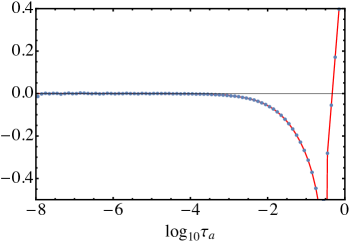
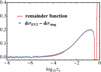
Figure 3: Top: Comparison of the EVENT2 prediction for two angularity distributions at $\mathcal{O}(\alpha_{s})$ with the analytically-known singular terms that follow from Eq. (52). Bottom: Comparison of their difference with the remainder function $r^{1}(\tau_{a})$ from Hornig:2009vb .

In the limit of zero bin size, EVENT2 is generating an approximation to the differential distribution, which takes the form:

$$\frac{1}{\sigma_{0}}\frac{d\sigma}{d\tau_{a}}=A\,\delta(\tau_{a})+[B(\tau_{a})]_{+}+r(\tau_{a})\,,$$ (57)

where $A$ is the constant coefficient of the delta function, $B$ is a singular function, turned into an integrable plus-distribution, and $r=dr_{c}/d\tau_{a}$ is nonsingular, that is, directly integrable as $\tau_{a}\to 0$. However, in practice we only obtain the distribution away from $\tau_{a}=0$ from EVENT2, thus obtaining a histogram of the function:

$$\frac{1}{\sigma_{0}}\frac{d\sigma}{d\tau_{a}}\biggr{\rvert}_{\tau_{a}>0}=B(\tau_{a})+r(\tau_{a})\,.$$ (58)

The delta function coefficient $A$, which gives the constants $c_{n0}$ in the integrated distribution Eq. (55), does not appear. The SCET prediction, on the other hand, gives just the singular parts:

$$\frac{1}{\sigma_{0}}\frac{d\sigma_{\text{sing}}}{d\tau_{a}}=A\,\delta(\tau_{a})+[B(\tau_{a})]_{+}\,,$$ (59)

so the difference between the EVENT2 and SCET predictions (away from $\tau_{a}=0$) gives the nonsingular part:

$$\frac{1}{\sigma_{0}}\frac{d\sigma}{d\tau_{a}}-\frac{1}{\sigma_{0}}\frac{d\sigma_{\text{sing}}}{d\tau_{a}}\;\biggr{\rvert}_{\tau_{a}>0}=r(\tau_{a})=\frac{\alpha_{s}(Q)}{2\pi}r^{1}(\tau_{a})+\Bigl{(}\frac{\alpha_{s}(Q)}{2\pi}\Bigr{)}^{2}r^{2}(\tau_{a})\,.$$ (60)

Integrating this difference over $0<\tau_{a}\leq 1$ then gives the expansion of the nonsingular part in terms of the $r_{c}^{n}$ functions in Eq. (55):

$$\lim_{\tau_{a}\to 0}\,\int_{\tau_{a}}^{1}d\tau_{a}^{\prime}\,r(\tau_{a}^{\prime})=r_{c}(1)=\frac{\alpha_{s}(Q)}{2\pi}r_{c}^{1}(1)+\Bigl{(}\frac{\alpha_{s}(Q)}{2\pi}\Bigr{)}^{2}r_{c}^{2}(1)\,.$$ (61)

Now, the total hadronic cross section, normalized to $\sigma_{0}$, is simply the integrated distribution Eq. (55) evaluated at $\tau_{a}=1$. As the plus-distributions integrate to zero over this region, we use Eq. (57) to obtain

$$\sigma_{\text{tot}}=A+r_{c}(1)\,.$$ (62)

The total cross section

$$\sigma_{\text{tot}}=1+\frac{\alpha_{s}(Q)}{2\pi}\,\sigma^{(1)}_{\text{tot}}+\Bigl{(}\frac{\alpha_{s}(Q)}{2\pi}\Bigr{)}^{2}\sigma^{(2)}_{\text{tot}}$$ (63)

is known to the considered order from Chetyrkin:1979bj ; Dine:1979qh ; Celmaster:1979xr :

$$\begin{split}\sigma^{(1)}_{\text{tot}}&=\frac{3}{2}C_{F}\,,\\ \sigma^{(2)}_{\text{tot}}&=-\frac{3}{8}C_{F}^{2}+\Bigl{(}\frac{123}{8}-11\zeta_{3}\Bigr{)}C_{F}C_{A}+\Bigl{(}-\frac{11}{2}+4\zeta_{3}\Bigr{)}C_{F}T_{F}n_{f}\,.\end{split}$$ (64)

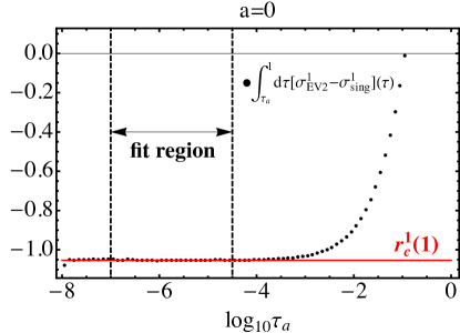
Figure 4: Integral Eq. (61) of the $\mathcal{O}(\alpha_{s})$ remainder function from EVENT2 as a function of the lower integration limit $\tau_{a}$. As $\tau_{a}\to 0$, a suitable fitting region is indicated that gives the constant $r_{c}^{1}(1)$, for the case $a=0$.

From the perturbative expansion of Eq. (62), we then obtain the relations

$$\begin{split}\sigma^{(1)}_{\text{tot}}&=c_{10}+r_{c}^{1}(1)\,,\\ \sigma^{(2)}_{\text{tot}}&=c_{20}+r_{c}^{2}(1)\,.\end{split}$$ (65)

The coefficient $c_{20}$ is precisely the constant $c^{(2)}$ in Eq. (53), so we can use Eq. (65) to determine $c^{(2)}$—and thus $c_{\tilde{J}}^{2}$ through Eq. (54)—from the known $\sigma^{(2)}_{\text{tot}}$ in Eq. (64) and the EVENT2 results for $r_{c}^{2}(1)$.

Essentially, the method relies on the fact that the total cross section is the sum of the singular constant $A$ and the integral over the nonsingular distribution $r_{c}(1)$. Summing the EVENT2 bins, with the singular terms subtracted off, between a small $\tau_{a}\sim 0$ and $\tau_{a}=1$ gives the latter. Its difference from the known total cross section then gives the singular constants $c_{n0}$.

This is illustrated for the $\mathcal{O}(\alpha_{s})$ parts of the differential distributions in Figs. 3 and 4. The EVENT2 data for these plots is based on $1\cdot 10^{11}$ events with a cutoff parameter of $10^{-12}$. In the upper plots of Fig. 3 we show the output of EVENT2 for two values of the angularity parameter, $a=-0.5$ and $a=0.5$, compared to the known predictions for the singular terms. The difference is shown in the lower plots of Fig. 3 together with the remainder function $r^{1}(\tau_{a})$ from Hornig:2009vb . One sees that the difference between the EVENT2 output and the singular terms vanishes as $\tau_{a}\to 0$ as expected. In Fig. 4 we show the result of computing the integral Eq. (61) as a sum over EVENT2 bins, for $a=0$. The value of this integral as the lower limit $\tau_{a}\to 0$ gives the numerical result for the constant $r_{c}^{1}(1)$, which through Eq. (65) gives an extraction of the singular constant $c_{10}$ in the fixed-order distribution. The $\mathcal{O}(\alpha_{s})$ terms are, of course, already known; we show this just to illustrate the logic of our procedure.

$a=-0.5$
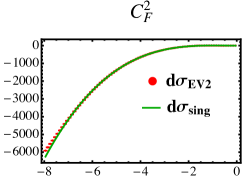
$a=0.5$

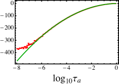
Figure 5: Comparison of the EVENT2 prediction for two angularity distributions at $\mathcal{O}(\alpha_{s}^{2})$ with the analytically-known singular terms that follow from Eq. (53). The plots show the coefficients of the color structures $C_{F}^{2}$, $C_{F}C_{A}$, $C_{F}T_{F}n_{f}$.

$a=-1$
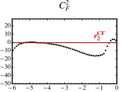
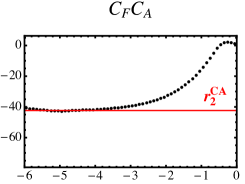
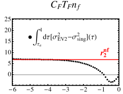
$a=-0.75$
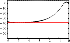
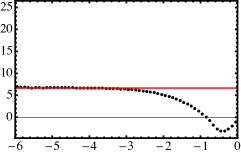
$a=-0.5$
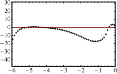
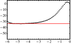
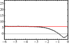
$a=-0.25$
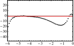
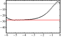
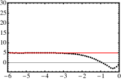
$a=0$
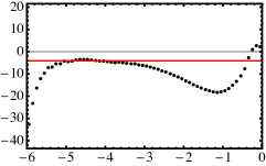
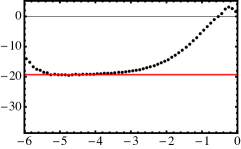
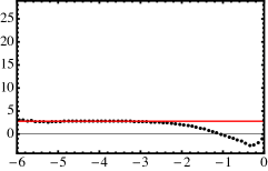
$a=0.25$
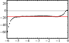
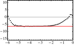
$a=0.5$

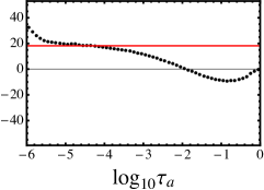
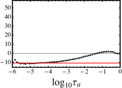
Figure 6: Integral Eq. (61) of the $\mathcal{O}(\alpha_{s}^{2})$ remainder function from EVENT2 as a function of the lower integration limit $\tau_{a}$. Shown are the coefficients of the $C_{F}^{2}$, $C_{F}C_{A}$, $C_{F}T_{F}n_{f}$ colour structures. Our best fit values for the constants $r_{2}^{CF},r_{2}^{CA},r_{2}^{nf}$ defined in Eq. (66) are shown in red.

Our EVENT2 results for the $\mathcal{O}(\alpha_{s}^{2})$ parts of the differential distributions are displayed for $a=-0.5$ and $a=0.5$ in Fig. 5. The functions plotted are the coefficients of the color structures $C_{F}^{2}$, $C_{F}C_{A}$, $C_{F}T_{F}n_{f}$, and the EVENT2 output is again shown in comparison to the singular terms predicted by Eq. (51). The agreement looks very good down to small values of $\tau_{a}$, until one gets so low that cutoff effects in EVENT2 play a role. For these plots we have again set the cutoff parameter to $10^{-12}$, and the results are based this time on $4\cdot 10^{10}$ events. The difference between the EVENT2 output and the singular terms is the nonsingular remainder function $r^{2}(\tau_{a})$, which we will show in Sec. 3.3. Integrating this difference according to Eq. (61) gives the numerical result for the integral $r_{c}^{2}(1)$. The relevant plots for computing these integrals as a sum over EVENT2 bins are shown in Fig. 6, and the values we extract for $r_{c}^{2}(1)$ are listed in Table 3. The tabulated results are the coefficients of each color structure:

$$r_{c}^{2}(1)=r_{2}^{CF}C_{F}^{2}+r_{2}^{CA}C_{F}C_{A}+r_{2}^{nf}C_{F}T_{F}n_{f}\,.$$ (66)

The errors we report on the extracted central values are determined by the values of the fitted parameters at which the $\chi^{2}$ per degree of freedom increases by 100% relative to that at the best fit value over the fit range of $\log_{10}\!\tau_{a}\in(-5+4a/10,-4+4a/10)$ for $C_{F}^{2}$, $\log_{10}\!\tau_{a}\in(-5,-4)$ for $C_{F}C_{A}$, and $\log_{10}\!\tau_{a}\in(-4.5,-3.5)$ for $C_{F}T_{F}n_{f}$, which we determined empirically by looking for stable plateau regions in Fig. 6 from which to perform the fits. These plateaus are very stable for the $C_{F}C_{A}$ and $C_{F}T_{F}n_{f}$ color structures for most values of $a$, but less so for many of the $C_{F}^{2}$ results — stability issues with $C_{F}^{2}$ singular terms in EVENT2 have been encountered in prior analyses as well (e.g. Chien:2010kc ; Chien:2015cka ). This is possibly due to an undersampling of $C_{F}^{2}$ contributions in the infrared region. Also from Fig. 6 it can be seen that we did not achieve stable plateaus for $a=0.5$ (except arguably for $C_{F}T_{F}n_{f}$) before hitting the cutoff-affected region. However we went ahead and applied the same fit procedure as described above, and the result in Table 4 for $a=0.5$ correspondingly has a much larger uncertainty. Despite these issues with $C_{F}^{2}$ and $a=0.5$ contributions, for our present analysis we were nevertheless able to obtain sufficiently reliable results for the final cross sections we present in Sec. 6. Namely, even doubling the uncertainties on $c_{\tilde{J}}^{2}$ shown in Table 4, the total NNLL^′ uncertainty bands on the cross sections in Sec. 6 are unchanged for all $a\leq 0.25$, and only change a few percent for $a=0.5$ in the resummation region, with the methods for uncertainty estimation described in Sec. 5.2. Of course, when other theoretical uncertainties are pushed sufficiently low to make the uncertainties on $r_{2}^{CF}$ and for $a=0.5$ more prominent (and before making a robust uncertainty estimate on any definitive extraction of $\alpha_{s}$), one should revisit the methods used to compute these numbers.

$a$	$-1.0$	$-0.75$	$-0.5$	$-0.25$	0.0	0.25	0.5
$r_{2}^{CF}$	$-0.16_{-0.28}^{+0.37}$	$0.19_{-0.24}^{+0.34}$	$0.24_{-0.18}^{+0.35}$	$-0.66_{-0.29}^{+0.36}$	$-4.03_{-0.27}^{+0.38}$	$-15.9_{-0.7}^{+0.4}$	$-49.9_{-8.4}^{+3.2}$
$r_{2}^{CA}$	$-42.3_{-0.5}^{+0.2}$	$-38.0_{-0.5}^{+0.2}$	$-33.2_{-0.3}^{+0.1}$	$-27.3_{-0.2}^{+0.1}$	$-19.3_{-0.2}^{+0.1}$	$-6.42_{-0.11}^{+0.20}$	$18.1_{-0.5}^{+1.5}$
$r_{2}^{nf}$	$6.76_{-0.03}^{+0.08}$	$6.57_{-0.03}^{+0.08}$	$6.03_{-0.03}^{+0.07}$	$4.92_{-0.02}^{+0.06}$	$2.78_{-0.02}^{+0.03}$	$-1.42_{-0.06}^{+0.02}$	$-9.92_{-0.87}^{+0.23}$

Table 3: Fit values for the coefficients of the integral $r_{c}^{2}(1)$ of the nonsingular QCD distribution as defined in Eq. (66). The central values and their uncertainties have been extracted from the plots in Fig. 6 as described in the text.

$a$	$-1.0$	$-0.75$	$-0.5$	$-0.25$	0.0	0.25	0.5
$c_{\tilde{J}}^{2}$	$66.0_{-3.4}^{+5.2}$	$42.3_{-3.3}^{+5.1}$	$17.3_{-2.5}^{+3.2}$	$-9.34_{-2.48}^{+2.76}$	$-36.3_{-2.4}^{+2.7}$	$-57.6_{-3.2}^{+3.8}$	$-79.8_{-24.9}^{+39.7}$

Table 4: Extracted values of the two-loop jet function constants $c_{\tilde{J}}^{2}$, determined by Eq. (54) and the value for $c^{(2)}$ implied by Eq. (67) and the numerical results for $r_{c}^{2}(1)$ in Table 3.

The constant part of the singular $\mathcal{O}(\alpha_{s}^{2})$ cross section is finally given by Eq. (65),

$$c^{(2)}\equiv c_{20}=\sigma^{(2)}_{\text{tot}}-r_{c}^{2}(1)\,,$$ (67)

which we can plug into Eq. (54) to obtain the so-far unknown two-loop jet function constant $c_{\tilde{J}}^{2}$. Our results are shown in Table 4, where we have set $n_{f}=5$ and we have added the uncertainties of the individual $r_{c}^{2}(1)$ coefficients in Table 3 linearly. In our phenomenological analysis below, we will vary $c_{\tilde{J}}^{2}$ over the uncertainties shown in Table 4, and we will account for its contribution to the overall uncertainties presented in Sec. 6. This particular contribution to the total uncertainty turns out, however, to be almost negligible. Our fit result for $a=0$ agrees well with the analytically known result from Becher:2006qw , $c_{\tilde{J}}^{2}=-36.3$.

3.3 Remainder functions

Figure 7: Left: $\mathcal{O}(\alpha_{s})$ remainder function for $a=0.25$, which is known from Hornig:2009vb . Right: The corresponding $\mathcal{O}(\alpha_{s}^{2})$ remainder function from EVENT2 (data points) with a suitable interpolation as described in the text.

We next move on to the integrable remainder function $r^{2}(\tau_{a})$ in Eq. (60), and consequently its nonsingular integrated version $r_{c}^{2}(\tau_{a})$ in Eq. (55). A prior issue to sort out in this context is the kinematic endpoint of the $\tau_{a}$ distribution in full QCD, which the singular predictions from SCET do not “see” since they assume $\tau_{a}\ll\tau_{a}^{\text{max}}\sim 1$.

The full QCD distribution $d\sigma/d\tau_{a}$ in Eq. (57) vanishes at $\mathcal{O}(\alpha_{s}^{k})$ above the maximum kinematic value of $\tau_{a}$ for $(k+2)$ particles in the final state, which we will call $\tau_{a}^{k,\text{max}}$. The SCET distribution $d\sigma_{\text{sing}}/d\tau_{a}$, however, continues above $\tau_{a}>\tau_{a}^{k,\text{max}}$ at this order. The remainder distribution $r(\tau_{a})$ in Eq. (60) is therefore just the negative of the SCET distribution above $\tau_{a}^{k,\text{max}}$:

$$r^{k}(\tau_{a})=\theta(\tau_{a}^{k,\text{max}}-\tau_{a})\,r^{k}(\tau_{a})-\theta(\tau_{a}-\tau_{a}^{k,\text{max}})\,B^{k}(\tau_{a})\,,$$ (68)

where $B^{k}$ is the $\mathcal{O}(\alpha_{s}^{k})$ coefficient of the singular distribution $B(\tau_{a})$ in Eq. (57) (in units of $(\alpha_{s}(Q)/(2\pi))^{k}$), and we have slightly abused notation in using the same symbol $r^{k}$ for the remainder function for $\tau_{a}<\tau_{a}^{k,\text{max}}$.

At $\mathcal{O}(\alpha_{s})$ there are up to three particles in the final state. The maximum value of $\tau_{a}$ occurs for the symmetric “Mercedes-star” configuration with three particles in a plane, with equal energy $E_{1,2,3}=Q/3$ and an angle $\theta_{ij}=2\pi/3$ between any two of them (for the values of $a$ we consider, but see Hornig:2009vb for exceptions). The thrust axis may then be taken to be along any of the three particles, and one easily derives $\tau_{a}^{1,\text{max}}=(1/3)^{1-a/2}$.

At $\mathcal{O}(\alpha_{s}^{2})$ there are up to four particles in the final state, and it is similarly straightforward to compute the angularity $\tau_{a}$ for the symmetric four-particle configuration, which we derive in App. D. Assuming that the symmetric configuration again determines the maximum for the values of $a$ relevant for our analysis, we obtain

$$\tau_{a}^{2,\text{max}}=\Bigl{(}1-\frac{\sqrt{3}}{3}\Bigr{)}^{1-a}\Bigl{(}\frac{2}{3}\Bigr{)}^{a/2}\,.$$ (69)

$a$	$-1$	$-0.75$	$-0.5$	$-0.25$	0	0.25	0.5
$a_{1}$	$6212$	$5401$	$4328$	$3526$	$1475$	$-209$	$22756$
$a_{2}$	1377	1210	986	803	343	50.8	6262
$a_{3}$	94.4	82.5	67.3	54.2	23.5	14.0	512
$b_{2}$	$-1680$	$-1139$	$-518$	$-491$	$-25.4$	793	4440
$b_{3}$	$-2455$	$-2098$	$-1619$	$-1317$	$-465$	423	$-7037$
$a_{0}$	5634	4694	3516	2884	1083	$-598$	14658

Table 5: Results for the fit coefficients in Eq. (71) obtained from the EVENT2 data displayed in Fig. 8. The uncertainties on these fits are illustrated in the plots on the right panel of Fig. 8.

$a=-1$
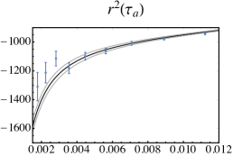
$a=-0.75$
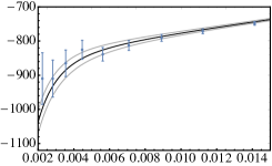
$a=-0.5$
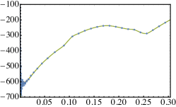
$a=-0.25$
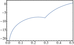
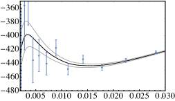
$a=0$
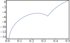
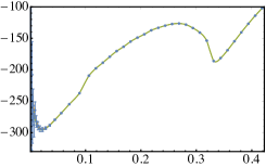
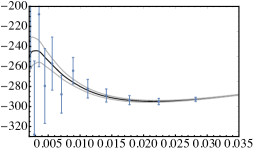
$a=0.25$
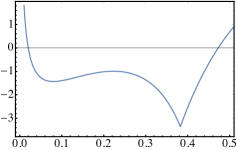
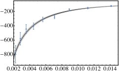
$a=0.5$

Figure 8: Left: $\mathcal{O}(\alpha_{s})$ remainder functions from Hornig:2009vb . Middle: $\mathcal{O}(\alpha_{s}^{2})$ remainder functions across the whole physical spectrum. Right: Magnified plots of the latter in the low $\tau_{a}$ region. Note that the vertical scales differ significantly across the plots, affecting the visual appearance of the uncertainty bands’ actual widths.

We next turn to the functional form of the remainder functions $r^{1}(\tau_{a})$ and $r^{2}(\tau_{a})$, which are displayed in Fig. 7 for $a=0.25$. For these results we collect EVENT2 data from all events at cutoffs of $10^{-12}$ and $10^{-15}$ as mentioned above. In the left panel the predicted curve from Hornig:2009vb for the $\mathcal{O}(\alpha_{s})$ remainder function is shown, whereas our EVENT2 results at $\mathcal{O}(\alpha_{s}^{2})$ are given by the data points in the right panel. In this panel we also illustrate how, following Abbate:2010xh , we divide the $\tau_{a}$ domain into two regions $\tau_{a}<0.1$ and $\tau_{a}>0.1$, where we bin linearly in $\log_{10}\tau_{a}$ or in $\tau_{a}$ itself, respectively, to accurately capture the shape of the remainder function across the whole domain. In the linearly binned region, the EVENT2 uncertainties are negligible and we take a direct interpolation of the data points to be our working remainder function. In the low $\tau_{a}$ region, on the other hand, we perform a fit to a predetermined basis of functions and use the result as our functional prediction. We then join these predictions smoothly to determine the final remainder function entering our cross section predictions:

$$r^{2}(\tau_{a}) =[1-f(\tau_{a},0.05,0.01)]\,r^{2}_{\log}(\tau_{a})+f(\tau_{a},0.05,0.01)\,r^{2}_{\text{lin}}(\tau_{a})\,,$$ (70)

with $f(z,z_{0},\epsilon)=1/(1+e^{-(z-z_{0})/\epsilon})$. We actually transition to the direct interpolation of the EVENT2 data $r^{2}_{\text{lin}}$ at $\tau_{a}=0.05$, which is a bit below the boundary $\tau_{a}=0.1$ between the logarithmically and linearly binned regions, since the EVENT2 data is so precise well below this point anyway.

The basis of functions we use to fit the data in the low $\tau_{a}$ region is given by

$$r^{2}_{\log}(\tau_{a})=a_{0}+a_{1}\ln\tau_{a}+a_{2}\ln^{2}\tau_{a}+a_{3}\ln^{3}\tau_{a}+b_{2}\,\tau_{a}\ln^{2}\tau_{a}+b_{3}\,\tau_{a}\ln\tau_{a}\,,$$ (71)

which is meant to be a representative but not necessarily complete (or even fully accurate) set of functions that can appear in the fixed-order $\mathcal{O}(\alpha_{s}^{2})$ distribution. This basis is simply chosen since it gives a good fit to the growth of $r^{2}(\tau_{a})$ at small values of $\tau_{a}$ to the accuracy of the EVENT2 data that we have. The fit is performed subject to the constraint that the total area $r_{c}^{2}(1)$ under the remainder function $r^{2}(\tau_{a})$ is consistent with the values extracted in Table 3. We just use the central values from that table, as varying it within the ranges shown gives a negligible shift in the extracted fit parameters in Eq. (71). The errors on our remainder function $r^{2}(\tau_{a})$ actually come from the 1-$\sigma$ error bands determined by the NonlinearModelFit routine in Mathematica, with the weight of each data point inversely proportional to the square of its EVENT2 error bar, and with $a_{0}$ determined by the area condition, leaving five free parameters in the fit. We give the results of these fits in Table 5.

Our final results for the $\mathcal{O}(\alpha_{s})$ and $\mathcal{O}(\alpha_{s}^{2})$ remainder functions for all seven values of the angularity $a$ we consider in this work are shown in Fig. 8. The uncertainties of the aforementioned fit procedure are hardly visible in the plots in the middle panel of Fig. 8, but they become noticeable in the low $\tau_{a}$ region, which is magnified in the right panel. Although the statistical errors from EVENT2 at low $\tau_{a}$ grow substantially, the fits are constrained by the highly precise larger $\tau_{a}$ data and the constraint on the total area under the remainder function. More precise results for $r^{2}(\tau_{a})$ at low $\tau_{a}$, and a more rigorous derivation of the fit functions that should appear in Eq. (71), are certainly desirable for precision phenomenology in this region, but such exercises lie outside the scope of this paper. Here we seek only to obtain sufficiently smooth and stable visual results for very low $\tau_{a}$ values, and focus on precision comparisons to data for intermediate-to-large $\tau_{a}$.

The remainder functions $r^{1}(\tau_{a})$ and $r^{2}(\tau_{a})$ have been extracted at a scale $\mu=Q$, cf. Eq. (55). The singular parts predicted by the factorization theorem Eq. (2.1) and these non-singular parts must separately add up to be scale independent, if summed to all orders in $\alpha_{s}(\mu)$. Thus we can probe the perturbative uncertainty of the non-singular parts by varying them as a function of a separate scale $\mu_{\text{ns}}$:

$$r(\tau_{a},\mu_{\text{ns}}) =r^{(1)}(\tau_{a},\mu_{\text{ns}})+r^{(2)}(\tau_{a},\mu_{\text{ns}})\,,$$ (72)

$$\text{where }r^{(1)}(\tau_{a},\mu_{\text{ns}}) \equiv\frac{\alpha_{s}(\mu_{\text{ns}})}{2\pi}\,r^{1}(\tau_{a})\,,$$

$$r^{(2)}(\tau_{a},\mu_{\text{ns}}) \equiv\Bigl{(}\frac{\alpha_{s}(\mu_{\text{ns}})}{2\pi}\Bigr{)}^{2}\Bigl{[}r^{2}(\tau_{a})+\beta_{0}\,r^{1}(\tau_{a})\ln\frac{\mu_{\text{ns}}}{Q}\Bigr{]}\,,$$

and similarly for the integrated version $r_{c}$. These functions $r(\tau_{a},\mu_{\text{ns}}),r_{c}(\tau_{a},\mu_{\text{ns}})$ enter our final NLL${}^{\prime}+\mathcal{O}(\alpha_{s})$, NNLL$+\mathcal{O}(\alpha_{s})$, and NNLL${}^{\prime}+\mathcal{O}(\alpha_{s}^{2})$ resummed and matched predictions for the cross sections we will present in Sec. 6. We have now assembled all the perturbative ingredients that we need to make these predictions. But before we do so, we turn our attention to the implementation of non-perturbative effects, whose proper treatment can even improve the behaviour of the perturbative convergence.

4 Non-perturbative corrections

Having resummed the angularity distributions in Sec. 2 and matched them to the fixed-order predictions in Sec. 3, we will now include a treatment of non-perturbative corrections that will influence the overall shape and position of the distributions.

4.1 Non-perturbative shape function

As with any hadronic observable, event shapes are sensitive to low energetic QCD radiation and effects of confinement. The importance of these non-perturbative effects depends on the domain of $\tau_{a}$ considered. For angularities with $a<1$, power corrections from the collinear sector are suppressed with respect to those from the soft sector Lee:2006nr ; Becher:2013iya . The non-perturbative effects can then be parameterized into a soft shape function $f_{\text{mod}}(k)$ that is convolved with the perturbative distribution Korchemsky:1998ev ; Korchemsky:1999kt ; Hoang:2007vb :

$$S(k,\mu)=\int dk^{\prime}\;S_{\text{PT}}(k-k^{\prime},\mu)\,f_{\text{mod}}(k^{\prime}-2\overline{\Delta}_{a})\,,$$ (73)

which ultimately leads to Eq. (4) for the cross section. Here $S_{\text{PT}}$ is the soft function computed in perturbation theory, and $\overline{\Delta}_{a}$ is a gap parameter, which we will address in the next subsection. The shape function $f_{\text{mod}}(k)$ is positive definite and normalized. We follow previous approaches and expand the shape function in a complete set of orthonormal basis functions Ligeti:2008ac :

$$f_{\text{mod}}(k)=\frac{1}{\lambda}\left[\sum_{n=0}^{\infty}\,b_{n}\,f_{n}\left(\frac{k}{\lambda}\right)\right]^{2}\,,$$ (74)

where

$$f_{n}(x) =8\sqrt{\frac{2x^{3}\left(2n+1\right)}{3}}\,e^{-2x}\,P_{n}\big{(}g(x)\big{)}\,,$$ (75)

$$g(x) =\frac{2}{3}\left(3-e^{-4x}\left(3+12x+24x^{2}+32x^{3}\right)\right)-1\,,$$

and $P_{n}$ are Legendre polynomials. The normalization of the shape function implies that the coefficients $b_{n}$ satisfy $\sum_{n=0}^{\infty}b_{n}^{2}=1$. In practice, we only keep one term in the sum (74), setting $b_{n}=0$ for $n>0$ (cf. Abbate:2010xh ; Hoang:2014wka ; Kang:2013nha ). The parameter $\lambda$ is then constrained by the first moment of the shape function as explained in the next subsection. More terms can in principle be included in Eq. (74) if one wishes to study higher non-perturbative moments beyond the first one.

This function, when convolved with the perturbative distribution from the previous sections, reproduces the known shift in the tail region Korchemsky:1994is ; Dokshitzer:1995zt ; Dokshitzer:1995qm , which can be shown rigorously via an operator product expansion (OPE) Lee:2006nr to be the dominant non-perturbative effect,

$$\frac{d\sigma}{d\tau_{a}}(\tau_{a})\underset{\text{NP}}{\longrightarrow}\frac{d\sigma}{d\tau_{a}}\Big{(}\tau_{a}-c_{\tau_{a}}\frac{\overline{\Omega}_{1}}{Q}\Big{)}\,.$$ (76)

Here $\overline{\Omega}_{1}$ is a universal non-perturbative parameter that is defined as a vacuum matrix element of soft Wilson lines and a transverse energy-flow operator (for details, see Lee:2006nr ). On the other hand, $c_{\tau_{a}}$ is an exactly calculable observable-dependent coefficient which, for the angularities, is given by $c_{\tau_{a}}=2/(1-a)$ Berger:2003pk ; Berger:2004xf ; Lee:2006nr .

4.2 Gap parameter and renormalon subtraction

As advocated in Hoang:2007vb , we use a soft function with a non-perturbative gap parameter $\overline{\Delta}_{a}$, as already displayed in Eq. (73). The gap parameter accounts for the minimum value of $\tau_{a}$ for a hadronic spectrum (the distribution can go down to zero for massless partons, but not for massive hadrons). In the tail region of the distributions, Eq. (73) then leads to a shift of the perturbative cross section, Eq. (76), with

$$\frac{2\overline{\Omega}_{1}}{1-a}=2\overline{\Delta}_{a}+\int dk\,k\,f_{\text{mod}}(k)\,.$$ (77)

Since the first moment is shifted linearly by $\overline{\Delta}_{a}$, this parameter was rescaled in Hornig:2009vb from its default definition in Hoang:2007vb via

$$\overline{\Delta}_{a}=\frac{\overline{\Delta}}{1-a}\,,$$ (78)

where $\overline{\Delta}\sim\Lambda_{\text{QCD}}$ is an $a$-independent parameter. Note that this determines that, with Eq. (74) truncated at $n=0$, the model function parameter $\lambda=2(\overline{\Omega}_{1}-\overline{\Delta})/(1-a)$. Up to this point, the barred quantities $\overline{\Omega}_{1},\overline{\Delta}_{(a)}$ are taken to be defined in a perturbative scheme like $\overline{\text{MS}}$ in which $S_{\text{PT}}$ has been calculated. In Hoang:2007vb it was pointed out that such a definition of the gap parameter $\overline{\Delta}_{a}$ has a renormalon ambiguity, shared by the perturbative soft function $S_{\text{PT}}$ in Eq. (73). This is similar but not identical to the renormalon in the pole mass for heavy quarks (see, e.g. Beneke:1994sw ). To obtain stable predictions, it is necessary to cancel the ambiguity from both $S_{\text{PT}}$ and $\overline{\Delta}_{a}$ in Eq. (73). This can be done by redefining the gap parameter as

$$\overline{\Delta}_{a}=\Delta_{a}(\mu)+\delta_{a}(\mu)\,,$$ (79)

where $\delta_{a}$ has a perturbative expansion with the same renormalon ambiguity as $S_{\text{PT}}$ (but opposite sign). The remainder $\Delta_{a}$ is then renormalon free, but its definition depends on the scheme and the scale of the subtraction term $\delta_{a}$. We adopt here the prescription chosen in Hoang:2008fs and also later implemented by Hornig:2009vb ; Abbate:2010xh ; Hoang:2014wka , which is based on the position-space subtraction for the heavy-quark pole-mass renormalon introduced in Jain:2008gb ; Hoang:2008yj . We will translate this notation to the Laplace-space soft function we have been using in this paper—see Eq. (34). The two formulations are completely equivalent with $\nu\leftrightarrow ix$.

The subtraction and its evolution equations are easier to formulate in Laplace space than in momentum space. For the Laplace-space soft function

$$\widetilde{S}(\nu,\mu)=\int_{0}^{\infty}dk\,e^{-\nu k}S(k,\mu)\,,$$ (80)

the convolution in Eq. (73) becomes

$$\widetilde{S}(\nu,\mu)=\Bigl{[}e^{-2\nu\Delta_{a}(\mu)}\widetilde{f}_{\text{mod}}(\nu)\Bigr{]}\Bigl{[}e^{-2\nu\delta_{a}(\mu)}\widetilde{S}_{\text{PT}}(\nu,\mu)\Bigr{]}\,,$$ (81)

where we have grouped the renormalon-free gap parameter $\Delta_{a}$ with the shape function $\widetilde{f}_{\text{mod}}$, and the perturbative subtraction term $\delta_{a}$ with $\widetilde{S}_{\text{PT}}$, rendering each group of terms in brackets renormalon free. There are a number of schemes one can choose to define $\delta_{a}$ that achieve cancellation of the leading renormalon. A particularly convenient one found in Jain:2008gb ; Hoang:2008yj ; Hoang:2008fs is a condition that fixes the derivative of the soft function at some value of $\nu$ to have an unambiguous value:

$$Re^{\gamma_{E}}\frac{d}{d\ln\nu}\Bigl{[}\ln\widehat{S}_{\text{PT}}(\nu,\mu)\Bigr{]}_{\nu=1/(Re^{\gamma_{E}})}=0\,,$$ (82)

where $\widehat{S}_{\text{PT}}(\nu,\mu)=e^{-2\nu\delta_{a}(\mu)}\widetilde{S}_{\text{PT}}(\nu,\mu)$, which is sufficient to render $\widehat{S}_{\text{PT}}$, and thus $\Delta_{a}$, to be renormalon-free. This is known as the “Rgap” scheme, and its condition determines $\delta_{a}$ as a function of a new, arbitrary subtraction scale $R$, which should be taken to be perturbative, but small enough to describe the characteristic fluctuations in the soft function. Explicitly, Eq. (82) defines the subtraction term as

$$\delta_{a}(\mu,R)=\frac{1}{2}Re^{\gamma_{E}}\frac{d}{d\ln\nu}\Bigl{[}\ln\widetilde{S}_{\text{PT}}(\nu,\mu)\Bigr{]}_{\nu=1/(Re^{\gamma_{E}})}\,,$$ (83)

and we see that $\delta_{a}$ (and thus $\Delta_{a}$) depends on two perturbative scales, $\mu$ and $R$. Expanding the subtraction terms as

$$\delta_{a}(\mu,R)=Re^{\gamma_{E}}\biggl{[}\frac{\alpha_{s}(\mu)}{4\pi}\delta_{a}^{1}(\mu,R)+\Bigl{(}\frac{\alpha_{s}(\mu)}{4\pi}\Bigr{)}^{2}\delta_{a}^{2}(\mu,R)+\cdots\biggr{]}\,,$$ (84)

we obtain, for the $\overline{\text{MS}}$ Laplace-space soft function $\widetilde{S}_{\text{PT}}$, using its expansion in Eq. (34),

$$\delta_{a}^{1}(\mu,R) =\Gamma_{S}^{0}\ln\frac{\mu}{R}\,,$$ (85a)

$$\delta_{a}^{2}(\mu,R) =\Gamma_{S}^{0}\beta_{0}\ln^{2}\frac{\mu}{R}+\Gamma_{S}^{1}\ln\frac{\mu}{R}+\frac{\gamma_{S}^{1}(a)}{2}+c_{\tilde{S}}^{1}(a)\beta_{0}\,,$$ (85b)

where from Eq. (35), $\Gamma_{S}^{n}=-2\Gamma_{n}/(1-a)$, and $\gamma_{S}^{1}$ and $c_{\tilde{S}}^{1}$ are given by Eq. (38) and Eq. (42).

Eq. (85) exhibits logarithms of $\mu/R$ that appear in the subtraction term $\delta_{a}$ and thus the renormalon-free gap parameter $\Delta_{a}$. Since $\mu=\mu_{S}$ will be chosen in the next section to be a function of $\tau_{a}$, which varies over a large range between $\mu_{0}\sim 1\text{ GeV}$ and $Q$, a fixed value of $R$ can only minimize these logarithms in one region of $\tau_{a}$, but not everywhere. We therefore need to allow $R$ to vary as well to track $\mu_{S}$, and so we need to know the evolution of $\Delta_{a}$ in both $\mu$ and $R$. The $\mu$-RGE is simple to derive. Since $\overline{\Delta}_{a}$ in Eq. (79) is $\mu$-independent, we obtain

$$\mu\frac{d}{d\mu}\Delta_{a}(\mu,R)=-\mu\frac{d}{d\mu}\delta_{a}(\mu,R)\equiv\gamma_{\Delta}^{\mu}[\alpha_{s}(\mu)]\,,$$ (86)

where from the perturbative expansion of $\delta_{a}$ in Eq. (85), we can determine

$$\gamma_{\Delta}^{\mu}[\alpha_{s}(\mu)]=-Re^{\gamma_{E}}\Gamma_{S}[\alpha_{s}(\mu)]\,,$$ (87)

explicitly to $\mathcal{O}(\alpha_{s}^{2})$, and which can be shown to hold to all orders Hoang:2008fs . The solution of this RGE is given by

$$\Delta_{a}(\mu,R)=\Delta_{a}(\mu_{\Delta},R)+Re^{\gamma_{E}}\frac{\kappa_{S}}{2}\,\eta_{\Gamma}(\mu,\mu_{\Delta})\,,$$ (88)

with an initial condition at some scale $\mu_{\Delta}$, and where $\kappa_{S}=4/(1-a)$ was given in Eq. (14) and the kernel $\eta_{\Gamma}$ was defined in Eq. (13).

The evolution of the gap parameter $\Delta_{a}(\mu,R)$ in $R$ is a bit more involved, and was solved in Hoang:2008yj for quark masses and applied to the soft gap parameter in Hoang:2008fs . We follow this derivation here (in our own notation). Since from Eq. (88) we know how to evolve $\Delta_{a}(\mu,R)$ in $\mu$, we just need to derive the evolution of $\Delta_{a}(R,R)$ in $R$. Since $\overline{\Delta}_{a}$ in Eq. (79) is also $R$-independent, we can derive from the perturbative expansion of $\delta_{a}$ in Eq. (85) the “$R$-evolution” equation:

$$\frac{d}{dR}\,\Delta_{a}(R,R)=-\frac{d}{dR}\,\delta_{a}(R,R)\equiv-\gamma_{R}[\alpha_{s}(R)]\,,$$ (89)

where $\gamma_{R}$ has a perturbative expansion,

$$\gamma_{R}[\alpha_{s}(R)]=\sum_{n=0}^{\infty}\Bigl{(}\frac{\alpha_{s}(R)}{4\pi}\Bigr{)}^{n+1}\gamma_{R}^{n}\,,$$ (90)

whose first two coefficients we read off from Eqs. (84) and (85),

$$\gamma_{R}^{0}=0\,,\quad\gamma_{R}^{1}=\frac{e^{\gamma_{E}}}{2}\bigl{[}\gamma_{S}^{1}(a)+2c_{\widetilde{S}}^{1}\beta_{0}\bigr{]}\,.$$ (91)

Even though $\gamma_{R}^{0}=0$ for the soft gap parameter (since $\gamma_{S}^{0}(a)=0$), we will keep it symbolically in the solution below for generality (and for direct comparison with the quark mass case in Hoang:2008yj ).

To solve Eq. (89), we integrate:

$$\Delta_{a}(R_{1},R_{1})-\Delta_{a}(R_{\Delta},R_{\Delta})=-\int_{R_{\Delta}}^{R_{1}}\frac{dR}{R}\,R\,\gamma_{R}[\alpha_{s}(R)]\,,$$ (92)

multiplying and dividing by $R$ in the integrand, anticipating using Eq. (27) to change integration variables to $\alpha_{s}$. But first we need to invert $\alpha_{s}(R)$ to express $R$. To this end, we write Eq. (27) in the form

$$\ln\frac{R}{R_{\Delta}}=\int_{\alpha_{s}(R_{\Delta})}^{\alpha_{s}(R)}\frac{d\alpha}{\beta[\alpha]}=G[\alpha_{s}(R)]-G[\alpha_{s}(R_{\Delta})]\,,$$ (93)

where $G[\alpha]$ is the antiderivative of $1/\beta[\alpha]$,

$$G^{\prime}[\alpha]=\frac{1}{\beta[\alpha]}=-\frac{2\pi}{\beta_{0}}\frac{1}{\alpha^{2}}\frac{1}{1+\frac{\alpha}{4\pi}\frac{\beta_{1}}{\beta_{0}}+\bigl{(}\frac{\alpha}{4\pi}\bigr{)}^{2}\frac{\beta_{2}}{\beta_{0}}+\cdots}\,.$$ (94)

This determines $G$ up to a constant of integration (we effectively choose it such that $G[\alpha]\to 0$ as $\alpha\to\infty$). If $R,R_{\Delta}$ are scales for which $\alpha_{s}$ is perturbative, we can determine $G$ explicitly order by order,

$$G[\alpha]=\frac{2\pi}{\beta_{0}}\biggl{[}\frac{1}{\alpha}+\frac{\beta_{1}}{4\pi\beta_{0}}\ln\alpha-\frac{B_{2}}{(4\pi)^{2}}\,\alpha+\cdots\biggr{]}\,,$$ (95)

with $B_{2}$ from Eq. (25). Then Eq. (93) gives $R$ in terms of any other perturbative scale $R_{\Delta}$ as

$$R=e^{G[\alpha_{s}(R)]}\Bigl{[}R_{\Delta}e^{-G[\alpha_{s}(R_{\Delta})]}\Bigr{]}\,,$$ (96)

and we can use this relation in Eq. (92) to achieve the change of variables from $R$ to $\alpha_{s}$,

$$\Delta_{a}(R_{1},R_{1})-\Delta_{a}(R_{\Delta},R_{\Delta})=-R_{\Delta}e^{-G[\alpha_{s}(R_{\Delta})]}\int_{\alpha_{s}(R_{\Delta})}^{\alpha_{s}(R_{1})}\frac{d\alpha}{\beta[\alpha]}\,e^{G[\alpha]}\,\gamma_{R}[\alpha]\,.$$ (97)

Keeping the explicit expression for $G$ in Eq. (95) up to the $B_{2}$ term, and expanding out the integrand in powers of $\alpha_{s}$ where we can, we obtain

$$\Delta_{a}(R_{1},R_{1})-\Delta_{a}(R_{\Delta},R_{\Delta})$$ (98)

$$\quad=\frac{R_{\Delta}}{2\beta_{0}}\,e^{-G[\alpha_{s}(R_{\Delta})]}\int_{\alpha_{s}(R_{\Delta})}^{\alpha_{s}(R_{1})}\frac{d\alpha}{\alpha}\,e^{\frac{2\pi}{\beta_{0}\alpha}}\;\alpha^{\frac{\beta_{1}}{2\beta_{0}^{2}}}\,\biggl{\{}\gamma_{R}^{0}+\frac{\alpha}{4\pi}\Bigl{[}\gamma_{R}^{1}-\frac{\gamma_{R}^{0}}{\beta_{0}}\Bigl{(}\beta_{1}+\frac{B_{2}}{2}\Bigr{)}\Bigr{]}+\cdots\biggr{\}}\,.$$

This series of integrals is conveniently evaluated by changing the integration variable to $t=-2\pi/(\beta_{0}\alpha)$, upon which

$$\Delta_{a}(R_{1},R_{1})-\Delta_{a}(R_{\Delta},R_{\Delta})$$ (99)

$$\quad=\frac{R_{\Delta}}{2\beta_{0}}\,e^{-G[\alpha_{s}(R_{\Delta})]}\,\Bigl{(}\frac{2\pi}{\beta_{0}}e^{i\pi}\Bigr{)}^{\frac{\beta_{1}}{2\beta_{0}^{2}}}\int_{t_{1}}^{t_{0}}\frac{dt}{t}\,e^{-t}\,t^{-\frac{\beta_{1}}{2\beta_{0}^{2}}}\biggl{\{}\gamma_{R}^{0}-\frac{1}{2\beta_{0}t}\Big{[}\gamma_{R}^{1}-\frac{\gamma_{R}^{0}}{\beta_{0}}(\beta_{1}+\frac{B_{2}}{2}\Bigr{)}\Bigr{]}+\cdots\biggr{\}}\,.$$

These integrals can then be expressed in terms of the incomplete gamma function $\Gamma(c,x)=\int_{x}^{\infty}dt\,t^{-1+c}\,e^{-t}$, such that

$$\Delta_{a}(R_{1},R_{1})-\Delta_{a}(R_{\Delta},R_{\Delta})$$ (100)

$$\quad=\frac{R_{\Delta}}{2\beta_{0}}\,e^{-G[\alpha_{s}(R_{\Delta})]}\,\Bigl{(}\frac{2\pi}{\beta_{0}}e^{i\pi}\Bigr{)}^{\frac{\beta_{1}}{2\beta_{0}^{2}}}\,\biggl{\{}\gamma_{R}^{0}\,\Bigl{[}\Gamma\Bigl{(}-\tfrac{\beta_{1}}{2\beta_{0}^{2}},-\tfrac{2\pi}{\beta_{0}\alpha_{s}(R_{1})}\Bigr{)}-\Gamma\Bigl{(}-\tfrac{\beta_{1}}{2\beta_{0}^{2}},-\tfrac{2\pi}{\beta_{0}\alpha_{s}(R_{\Delta})}\Bigr{)}\Bigr{]}$$

$$\qquad\!-\frac{1}{2\beta_{0}}\Bigl{[}\gamma_{R}^{1}-\frac{\gamma_{R}^{0}}{\beta_{0}}\Bigl{(}\beta_{1}\!+\!\frac{B_{2}}{2}\Bigr{)}\Bigr{]}\Bigl{[}\Gamma\Bigl{(}-\tfrac{\beta_{1}}{2\beta_{0}^{2}}\!-\!1,-\tfrac{2\pi}{\beta_{0}\alpha_{s}(R_{1})}\Bigr{)}-\Gamma\Bigl{(}-\tfrac{\beta_{1}}{2\beta_{0}^{2}}\!-\!1,-\tfrac{2\pi}{\beta_{0}\alpha_{s}(R_{\Delta})}\Bigr{)}\Bigr{]}\!+\cdots\!\biggr{\}}\,,$$

which is consistent with the solution of the $R$-evolution equation given in Hoang:2008yj ; Hoang:2008fs . The solution of both $\mu$- and $R$-evolution equations in Eqs. (88) and (100) finally determines the renormalon-subtracted gap parameter $\Delta_{a}(R,\mu)$ at any perturbative scales $R,\mu$ in terms of an input value $\Delta_{a}(R_{\Delta},R_{\Delta})$ at a reference scale $R_{\Delta}$:

$$\Delta_{a}(\mu,R)=\Delta_{a}(R_{\Delta},R_{\Delta})+Re^{\gamma_{E}}\frac{\kappa_{S}}{2}\,\eta_{\Gamma}(\mu,R)$$ (101)

$$\quad+\frac{R_{\Delta}}{2\beta_{0}}\,e^{-G[\alpha_{s}(R_{\Delta})]}\Bigl{(}\frac{2\pi}{\beta_{0}}e^{i\pi}\Bigr{)}^{\frac{\beta_{1}}{2\beta_{0}^{2}}}\,\biggl{\{}\gamma_{R}^{0}\Bigl{[}\Gamma\Bigl{(}-\tfrac{\beta_{1}}{2\beta_{0}^{2}},-\tfrac{2\pi}{\beta_{0}\alpha_{s}(R)}\Bigr{)}-\Gamma\Bigl{(}-\tfrac{\beta_{1}}{2\beta_{0}^{2}},-\tfrac{2\pi}{\beta_{0}\alpha_{s}(R_{\Delta})}\Bigr{)}\Bigr{]}$$

$$\qquad-\frac{1}{2\beta_{0}}\Bigl{[}\gamma_{R}^{1}-\frac{\gamma_{R}^{0}}{\beta_{0}}\Bigl{(}\beta_{1}\!+\!\frac{B_{2}}{2}\Bigr{)}\Bigr{]}\Bigl{[}\Gamma\Bigl{(}-\tfrac{\beta_{1}}{2\beta_{0}^{2}}\!-\!1,-\tfrac{2\pi}{\beta_{0}\alpha_{s}(R)}\Bigr{)}-\Gamma\Bigl{(}-\tfrac{\beta_{1}}{2\beta_{0}^{2}}\!-\!1,-\tfrac{2\pi}{\beta_{0}\alpha_{s}(R_{\Delta})}\Bigr{)}\Bigr{]}\!+\cdots\!\biggr{\}}\,.$$

This expression is real, and we recall that $\gamma_{R}^{0}=0$ in our case.

In the solution of the $\mu$- and $R$-evolution of $\Delta_{a}$ in Eq. (101), we truncate at each order of logarithmic accuracy as follows: at NLL(^′) we keep $\gamma_{\Delta}^{\mu},\gamma_{R}$ to $\mathcal{O}(\alpha_{s})$ (i.e. up to the second line of Eq. (101)), and at NNLL(^′) we keep $\gamma_{\Delta}^{\mu},\gamma_{R}$ to $\mathcal{O}(\alpha_{s}^{2})$ (i.e up to the last line). These rules are summarized with all other truncation rules in Table 6 below. Note that this means that $\eta_{\Gamma}$ is actually kept to one order of accuracy lower than indicated by Eq. (24). This is because the $\mu$-evolution of $\Delta_{a}$ in Eq. (88) is not multiplied by an extra logarithm as for the hard, jet, and soft functions in the full factorized cross section.

Transforming the renormalon-free soft function in Eq. (81) back to momentum space, we obtain the shifted version of Eq. (73),

$$S(k,\mu)=\int dk^{\prime}\;S_{\text{PT}}\bigl{(}k-k^{\prime}-2\delta_{a}(\mu,R),\mu\bigr{)}\,f_{\text{mod}}\bigl{(}k^{\prime}-2\Delta_{a}(\mu,R)\bigr{)}\,.$$ (102)

Then the parameter $\overline{\Omega}_{1}$ in Eq. (77), describing the non-perturbative shift of the perturbative cross section induced by the shape function, turns into a renormalon-free shift:

$$\frac{2\Omega_{1}(\mu,R)}{1-a}=2\Delta_{a}(\mu,R)+\int dk\,k\,f_{\text{mod}}(k)\,,$$ (103)

We will take the input gap parameter at a reference scale $R_{\Delta}=1.5\text{ GeV}$ to be $\Delta(R_{\Delta},R_{\Delta})=0.1$ GeV in our phenomenological analysis below. The exact value of this parameter is not particularly relevant to the tail region in which we focus our comparisons to data Abbate:2010xh .

The shift in the perturbative part of Eq. (102) can also be expressed in terms of a differential translation operator that acts on the perturbative soft function $S_{\text{PT}}$:

$$S(k,\mu)=\int dk^{\prime}\,\Bigl{[}e^{-2\delta_{a}(\mu,R)\frac{d}{dk}}\,S_{\text{PT}}\bigl{(}k-k^{\prime},\mu\bigr{)}\Bigr{]}\,f_{\text{mod}}\bigl{(}k^{\prime}-2\Delta_{a}(\mu,R)\bigr{)}\,,$$ (104)

which, after integrating by parts, gives

$$S(k,\mu)=\int dk^{\prime}\,S_{\text{PT}}\bigl{(}k-k^{\prime},\mu\bigr{)}\,\Bigl{[}e^{-2\delta_{a}(\mu,R)\frac{d}{dk^{\prime}}}\,f_{\text{mod}}\bigl{(}k^{\prime}-2\Delta_{a}(\mu,R)\bigr{)}\Bigr{]}\,.$$ (105)

In the final cross section, the renormalon-subtracted shape function then enters as a convolution against the perturbative distribution,

$$\frac{1}{\sigma_{0}}\,\sigma(\tau_{a})=\int dk\,\sigma_{\text{PT}}\Bigl{(}\tau_{a}-\frac{k}{Q}\Bigr{)}\Bigl{[}e^{-2\delta_{a}(\mu_{S},R)\frac{d}{dk}}f_{\text{mod}}\bigl{(}k-2\Delta_{a}(\mu_{S},R)\bigr{)}\Bigr{]}\,,$$ (106)

which is the expression we anticipated in Eq. (4). This implies we convolve both the singular and nonsingular parts of the cross section Eq. (6) with the same, renormalon-subtracted shape function. In doing this we follow Abbate:2010xh and ensure a smooth transition from the resummation to fixed-order regime even after non-perturbative effects are included.

In practice we expand out the shape function terms to the order we work in $\alpha_{s}$,

$$e^{-2\delta_{a}(\mu_{S},R)\frac{d}{dk}}f_{\text{mod}}(k-2\Delta_{a}(\mu_{S},R)) =f_{\text{mod}}^{(0)}(k-2\Delta_{a}(\mu_{S},R))+f_{\text{mod}}^{(1)}(k-2\Delta_{a}(\mu_{S},R))$$

$$\quad+f_{\text{mod}}^{(2)}(k-2\Delta_{a}(\mu_{S},R))\,,$$ (107)

where

$$f_{\text{mod}}^{(0)}(k-2\Delta_{a}(\mu_{S},R)) =f_{\text{mod}}(k-2\Delta_{a}(\mu_{S},R))\,,$$ (108a)

$$f_{\text{mod}}^{(1)}(k-2\Delta_{a}(\mu_{S},R)) =-\frac{\alpha_{s}(\mu_{S})}{4\pi}\,2\delta_{a}^{1}(\mu_{S},R)Re^{\gamma_{E}}f^{\prime}_{\text{mod}}(k-2\Delta_{a}(\mu_{S},R))\,,$$ (108b)

$$f_{\text{mod}}^{(2)}(k-2\Delta_{a}(\mu_{S},R)) =\Bigl{(}\frac{\alpha_{s}(\mu_{S})}{4\pi}\Bigr{)}^{2}\Bigl{[}-2\delta_{a}^{2}(\mu_{S},R)Re^{\gamma_{E}}f^{\prime}_{\text{mod}}(k-2\Delta_{a}(\mu_{S},R))$$ (108c)

$$\qquad\qquad+2(\delta_{a}^{1}(\mu_{S},R)Re^{\gamma_{E}})^{2}f^{\prime\prime}_{\text{mod}}(k-2\Delta_{a}(\mu_{S},R))\Bigr{]}\,,$$

with $\delta_{a}^{1,2}(\mu_{S},R)$ from Eq. (85). The order to which these terms are kept at each accuracy are included in Table 6.

Accuracy	$\Gamma_{\text{cusp}}$	$\gamma_{F},\gamma_{\Delta}^{\mu},\gamma_{R}$	$\beta$	$H,\tilde{J},\tilde{S},\delta_{a}$
LL	$\alpha_{s}$	1	$\alpha_{s}$	1
NLL	$\alpha^{2}_{s}$	$\alpha_{s}$	$\alpha^{2}_{s}$	1
NNLL	$\alpha^{3}_{s}$	$\alpha^{2}_{s}$	$\alpha^{3}_{s}$	$\alpha_{s}$
N3LL	$\alpha^{4}_{s}$	$\alpha^{3}_{s}$	$\alpha^{4}_{s}$	$\alpha^{2}_{s}$

Accuracy	$H,\tilde{J},\tilde{S},\delta_{a}$
NLL′	$\alpha_{s}$
NNLL′	$\alpha^{2}_{s}$
N3LL′	$\alpha^{3}_{s}$

Matching	$r^{n}(\tau_{a})$
$+\mathcal{O}(\alpha_{s})$	$\alpha_{s}$
$+\mathcal{O}(\alpha_{s}^{2})$	$\alpha^{2}_{s}$
$+\mathcal{O}(\alpha_{s}^{3})$	$\alpha^{3}_{s}$

Table 6: Ingredients we include at various orders of unprimed N^kLL (Left), primed N^kLL^′ (Middle), and matched (Right) accuracies, up to a given fixed order $\mathcal{O}(\alpha_{s}^{n})$. The tables apply to the integrated distribution in Eq. (110) and the Laplace-transformed distribution, but not, for unprimed accuracies, directly to the differential form in Eq. (2.1)—see Almeida:2014uva for details. We have included a counting for the renormalon subtractions terms $\delta_{a}$ in Eq. (84) and the $\mu$- and $R$-evolution anomalous dimensions $\gamma_{\Delta}^{\mu},\gamma_{R}$ in Eqs. (87) and (90) as described in the text.

4.3 Final resummed, matched, and renormalon-subtracted cross section

We now collect all pieces described above, giving our final expressions for the resummed cross section, matched to fixed-order and convolved with a renormalon-free shape function.

In evaluating the convolution in Eq. (106), we must truncate the product of the fixed-order perturbative pieces contained in Eqs. (17) and (60) along with the non-perturbative pieces in Eq. (4.2) to the appropriate order in $\alpha_{s}$ for N^kLL${}^{(^{\prime})}$ accuracy. Namely, starting with Eq. (17) for the integrated distribution, we expand the fixed-order coefficients in powers of $\alpha_{s}$:

$$\frac{\sigma_{c,\text{PT}}(\tau_{a})}{\sigma_{0}}=\sigma_{c}^{\text{LO}}(\tau_{a})+\sigma_{c}^{\text{NLO}}(\tau_{a})+\sigma_{c}^{\text{NNLO}}(\tau_{a})\,,$$ (109)

where

$$\sigma_{c}^{\text{N${}^{k}$LO}}(\tau_{a};\mu_{H},\mu_{J},\mu_{S},\mu_{\text{ns}}) =e^{\widetilde{K}(\mu_{H},\mu_{J},\mu_{S};Q)+K_{\gamma}(\mu_{H},\mu_{J},\mu_{S})}\Bigl{(}\frac{1}{\tau_{a}}\Bigr{)}^{\Omega(\mu_{J},\mu_{S})}$$ (110)

$$\quad\times\widetilde{F}_{k}(\tau_{a},\partial_{\Omega},\mu_{H},\mu_{J},\mu_{S})\;\frac{e^{\gamma_{E}\Omega}}{\Gamma(1-\Omega)}\ +\ r_{c}^{(k)}(\tau_{a},\mu_{\text{ns}})\,,$$

with the fixed-order operators $\widetilde{F}_{k}$ at each order given by

$$\widetilde{F}_{0}(\tau_{a},\partial_{\Omega},\mu_{H},\mu_{J},\mu_{S}) =1\,,$$ (111a)

$$\widetilde{F}_{1}(\tau_{a},\partial_{\Omega},\mu_{H},\mu_{J},\mu_{S}) =\frac{\alpha_{H}}{4\pi}H_{1}(Q^{2},\mu_{H})+2\frac{\alpha_{J}}{4\pi}\widetilde{J}_{1}\Bigl{(}\partial_{\Omega}+\ln\frac{\mu_{J}^{2-a}}{Q^{2-a}\tau_{a}},\mu_{J}\Bigr{)}$$ (111b)

$$\quad+\frac{\alpha_{S}}{4\pi}\widetilde{S}_{1}\Bigl{(}\partial_{\Omega}+\ln\frac{\mu_{S}}{Q\tau_{a}},\mu_{S}\Bigr{)}\,,$$

$$\widetilde{F}_{2}(\tau_{a},\partial_{\Omega},\mu_{H},\mu_{J},\mu_{S}) =\Bigl{(}\frac{\alpha_{H}}{4\pi}\Bigr{)}^{2}H_{2}(Q^{2},\mu_{H})+\Bigl{(}\frac{\alpha_{J}}{4\pi}\Bigr{)}^{2}(2\widetilde{J}_{2}+\widetilde{J}_{1}^{2})\Bigl{(}\partial_{\Omega}+\ln\frac{\mu_{J}^{2-a}}{Q^{2-a}\tau_{a}},\mu_{J}\Bigr{)}$$

$$\quad+\Bigl{(}\frac{\alpha_{S}}{4\pi}\Bigr{)}^{2}\widetilde{S}_{2}\Bigl{(}\partial_{\Omega}+\ln\frac{\mu_{S}}{Q\tau_{a}},\mu_{S}\Bigr{)}+\frac{\alpha_{H}}{4\pi}H_{1}(Q^{2},\mu_{H})$$ (111c)

$$\qquad\times\biggl{[}2\frac{\alpha_{J}}{4\pi}\widetilde{J}_{1}\Bigl{(}\partial_{\Omega}\!+\!\ln\frac{\mu_{J}^{2-a}}{Q^{2-a}\tau_{a}},\mu_{J}\Bigr{)}+\frac{\alpha_{S}}{4\pi}\widetilde{S}_{1}\Bigl{(}\partial_{\Omega}\!+\!\ln\frac{\mu_{S}}{Q\tau_{a}},\mu_{S}\Bigr{)}\biggr{]}$$

$$\quad+2\frac{\alpha_{J}}{4\pi}\frac{\alpha_{S}}{4\pi}\widetilde{J}_{1}\Bigl{(}\partial_{\Omega}\!+\!\ln\frac{\mu_{J}^{2-a}}{Q^{2-a}\tau_{a}},\mu_{J}\Bigr{)}\widetilde{S}_{1}\Bigl{(}\partial_{\Omega}\!+\!\ln\frac{\mu_{S}}{Q\tau_{a}},\mu_{S}\Bigr{)}\,,$$

where $\alpha_{F}\equiv\alpha_{s}(\mu_{F})$, $H_{n},\widetilde{J}_{n},\widetilde{S}_{n}$ are given by Eq. (34), and $r_{c}^{(k)}$ are the integrated versions of the remainder functions in Eq. (72) with $r_{c}^{(0)}(\tau_{a},\mu_{\text{ns}})=0$.

In the convolved cross section Eq. (106), the proper fixed-order expansion up to NNLL(^′) accuracy is then given by:

$$\frac{\sigma_{c}(\tau_{a})}{\sigma_{0}}=\sigma_{c}^{[0]}(\tau_{a})+\sigma_{c}^{[1]}(\tau_{a})+\sigma_{c}^{[2]}(\tau_{a})\,,$$ (112)

where

$$\sigma_{c}^{[0]}(\tau_{a}) =\int dk\;\sigma_{c}^{\text{LO}}\Bigl{(}\tau_{a}-\frac{k}{Q};\mu_{H},\mu_{J},\mu_{S}\Bigr{)}\,f_{\text{mod}}^{(0)}(k-2\Delta_{a}(\mu_{S},R))\,,$$ (113a)

$$\sigma_{c}^{[1]}(\tau_{a}) =\int dk\;\Bigl{\{}\sigma_{c}^{\text{NLO}}\Bigl{(}\tau_{a}-\frac{k}{Q};\mu_{H},\mu_{J},\mu_{S},\mu_{\text{ns}}\Bigr{)}\,f_{\text{mod}}^{(0)}(k-2\Delta_{a}(\mu_{S},R))$$ (113b)

$$\qquad\quad+\sigma_{c}^{\text{LO}}\Bigl{(}\tau_{a}-\frac{k}{Q};\mu_{H},\mu_{J},\mu_{S}\Bigr{)}\,f_{\text{mod}}^{(1)}(k-2\Delta_{a}(\mu_{S},R))\Bigr{\}}\,,$$

$$\sigma_{c}^{[2]}(\tau_{a}) =\int dk\;\Bigl{\{}\sigma_{c}^{\text{NNLO}}\Bigl{(}\tau_{a}-\frac{k}{Q};\mu_{H},\mu_{J},\mu_{S},\mu_{\text{ns}}\Bigr{)}\,f_{\text{mod}}^{(0)}(k\!-\!2\Delta_{a}(\mu_{S},R))$$ (113c)

$$\qquad\quad+\sigma_{c}^{\text{NLO}}\Bigl{(}\tau_{a}-\frac{k}{Q};\mu_{H},\mu_{J},\mu_{S},\mu_{\text{ns}}\Bigr{)}\,f_{\text{mod}}^{(1)}(k\!-\!2\Delta_{a}(\mu_{S},R))$$

$$\qquad\quad+\sigma_{c}^{\text{LO}}\Bigl{(}\tau_{a}-\frac{k}{Q};\mu_{H},\mu_{J},\mu_{S}\Bigr{)}\,f_{\text{mod}}^{(2)}(k-2\Delta_{a}(\mu_{S},R))\Bigr{\}}\,.$$

Eq. (112) is to be truncated at the fixed order demanded by Table 6 (first term up to NLL, second term for NLL^′ and NNLL, and up to the last term for NNLL^′), while the evolution kernels contained in each expression are to be evaluated to the appropriate resummed logarithmic accuracy as described in Sec. 2.

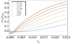
Figure 9: Predictions for the central values of the integrated cross sections at NNLL^′ accuracy in the low $\tau_{a}$ domain, shown here for seven values of the angularity parameter $a$. Left: Predictions from the purely perturbative cross section. Right: Predictions after renormalon subtraction as implemented in Eq. (113).

Eqs. (112) and (113) represent our final expression for the renormalon-free resummed and matched cross section that is convolved with a non-perturbative shape function. We should point out that we will perform the convolution in $k$ prior to choosing particular values for the scales $\mu_{H,J,S,\text{ns}}$ and $R$. We have clearly exhibited the dependence on these scales versus the explicit dependence on $\tau_{a}$ appearing in Eqs. (110) and (111). In the next section we will describe how we choose these scales, but for now it suffices to say that they are functions of the measured $\tau_{a}$ in the cross section, and not functions of the convolution variable $\tau_{a}-k/Q$. Thus the $\tau_{a}$ dependence inside the scales $\mu_{H,J,S,\text{ns}}$ and $R$ are not convolved over in Eq. (113). In our numerical code, the convolution between the explicit $\tau_{a}-k/Q$ dependence from Eqs. (110) and (111) and the $k$ dependence in $f_{\text{mod}}$ is then computed for a given set of scales $\mu_{i}(\tau_{a}),R(\tau_{a})$.

Fig. 9 illustrates the practical effect of implementing the renormalon subtraction and the convolution with the non-perturbative shape function as described above. We present the central theory curves at NNLL^′ accuracy for the cumulant cross sections at seven values of the parameter $a$, all in the low-$\tau_{a}$ domain. The curves in the left panel reflect the purely perturbative calculation, which exhibit unphysical (negative) values for the cross section. The curves in the right panel, on the other hand, represent the calculation performed with Eq. (113). It is clear that the renormalon cancellation is successful and no unphysical behavior is observed.

5 Scale choices

5.1 Profile functions

From the arguments of the logarithms in the fixed-order hard, jet, and soft functions appearing in Eq. (17), one can identify the natural scales at which these logarithms are minimized, finding

$$\mu_{H}^{\text{nat}}=Q,\,\,\,\,\,\,\,\mu_{J}^{\text{nat}}=Q\tau_{a}^{1/(2-a)},\,\,\,\,\,\,\,\mu_{S}^{\text{nat}}=Q\tau_{a}\,.$$ (114)

In the tail region, where the resummation is critical, we want to evaluate the distributions near these scales. However, we ultimately predict the distributions over a domain of $\tau_{a}$ that can be roughly broken into three regions where the comparative scalings differ (see, e.g. Abbate:2010xh ):

• Peak Region:     $\mu_{H}\gg\mu_{J}\gg\mu_{S}\sim\Lambda_{QCD}$ ,

• Tail Region:      $\mu_{H}\gg\mu_{J}\gg\mu_{S}\gg\Lambda_{QCD}$ ,

• Far-tail Region: $\mu_{H}=\mu_{J}=\mu_{S}\gg\Lambda_{QCD}$ .

In the peak region the soft scale is non-perturbative, and it is here that the full model shape function described in Sec. 4 becomes necessary for making reliable predictions. In this region we will adjust the scales to plateau at a constant value just above $\Lambda_{\text{QCD}}$. On the other hand, the scales are well separated in the tail region where the resummation is most important. We want to minimize the logarithms in the resummed distributions, and hence the scalings are close to the natural values in Eq. (114). Finally, our predictions should match onto fixed-order perturbation theory in the far-tail region. The resummations should therefore be switched off, and the scales should merge at $\mu_{H,J,S}\sim Q$.

Getting the scales to merge near $\mu_{H,J,S}\sim Q$ in the far-tail region will require $\mu_{J,S}$ to rise faster with $\tau_{a}$ than the natural scales in Eq. (114), since the physical maximum value of $\tau_{a}$ is less than 1. We will achieve this below by defining a smooth function to transition between the resummation and fixed-order regions. But the transition can be made less sudden by increasing the rate of change of $\mu_{J,S}$ even in the resummation region. Such an increased slope was used for the $C$-parameter and thrust distributions in Hoang:2014wka . For thrust, i.e. $a=0$, the authors used the central values

$$\mu_{S}=r_{s}\mu_{H}\tau_{0}\,,\qquad\mu_{J}=(\mu_{H}\mu_{S})^{1/2}\,,$$ (115)

with $r_{s}=2$ in the resummation region. We will follow this strategy here and give a physical interpretation to the slope parameter $r_{s}$. The maximal value for thrust is $\tau_{0}=1/2$, which is achieved for a perfectly spherically symmetric distribution of particles in the final state. The slope $r_{s}=2$ thus ensures that $\mu_{J,S}$ merge with $\mu_{H}$ at this maximum value $\tau_{0}^{\text{sph}}$, instead of at $\tau_{a}=1$ as the natural scales Eq. (114) do. For arbitrary $a$, the angularity of the spherically symmetric configuration is

$$\tau_{a}^{\text{sph}} =\frac{1}{4\pi}\int_{0}^{2\pi}d\phi\int_{-1}^{1}d\cos\theta\,\sin^{a}\theta(1-\left\lvert\cos\theta\right\rvert)^{1-a}=\frac{1}{2-\frac{a}{2}}\;{}_{2}F_{1}\Bigl{(}1,-\frac{a}{2};3-\frac{a}{2};-1\Bigr{)}\,,$$ (116)

which ranges from $\tau_{-1}^{\text{sph}}\approx 0.356$ to $\tau_{1/2}^{\text{sph}}\approx 0.616$ for the values of $a$ we consider in this work. These may be compared to the maximum values of a three- and four-particle configuration in Fig. 20 in App. D. We will then choose a default slope $r_{s}=1/\tau_{a}^{\text{sph}}$ in Eq. (115) that ensures that the scales $\mu_{H,J,S}$ meet at $\tau_{a}=\tau_{a}^{\text{sph}}$. We actually want the scales to merge a bit before $\tau_{a}^{\text{sph}}$, so that there is a non-vanishing region where the predicted distributions are purely fixed order.

We have designed a set of profile functions (see, e.g. Ligeti:2008ac ; Abbate:2010xh ; Kang:2014qba ; Hornig:2016ahz ) that fulfill all of the criteria discussed above while smoothly interpolating between the various regions. The precise form of our profiles depends on a running scale defined by

$$\mu_{\text{run}}(\tau_{a})=\begin{cases}\mu_{0}&\tau_{a}\leq t_{0}\\ \zeta\Big{(}\tau_{a};\{t_{0},\mu_{0},0\},\{t_{1},0,\frac{r}{\tau_{a}^{\text{sph}}}\mu_{H}\}\Big{)}&t_{0}\leq\tau_{a}\leq t_{1}\\ \frac{r}{\tau_{a}^{\text{sph}}}\,\mu_{H}\tau_{a}&t_{1}\leq\tau_{a}\leq t_{2}\\ \zeta\Big{(}\tau_{a};\{t_{2},0,\frac{r}{\tau_{a}^{\text{sph}}}\mu_{H}\},\{t_{3},\mu_{H},0\}\Big{)}&t_{2}\leq\tau_{a}\leq t_{3}\\ \mu_{H}&\tau_{a}\geq t_{3}\end{cases}\,.$$ (117)

The function $\zeta$ ensures that $\mu_{\text{run}}$ and its first derivative are smooth. Specifically, we adopt the functional form from Hoang:2014wka , which connects a straight line in the region $\tau_{a}<t_{0}$ with slope $r_{0}$ and intercept $y_{0}$ with another straight line in the region $\tau_{a}>t_{1}$ with slope $r_{1}$ and intercept $y_{1}$ via

$$\zeta\left(\tau_{a};\{t_{0},y_{0},r_{0}\},\{t_{1},y_{1},r_{1}\}\right)=\begin{cases}a+r_{0}(\tau_{a}-t_{0})+c(\tau_{a}-t_{0})^{2}&\tau_{a}\leq\frac{t_{0}+t_{1}}{2}\\ A+r_{1}(\tau_{a}-t_{1})+C(\tau_{a}-t_{1})^{2}&\tau_{a}\geq\frac{t_{0}+t_{1}}{2}\end{cases}\,,$$ (118)

where the coefficients of the polynomials are determined by continuity of the function and its first derivative:

$$a =y_{0}+r_{0}t_{0}\,, A =y_{1}+r_{1}t_{1}\,,$$ (119)

$$c =2\,\frac{A-a}{(t_{0}-t_{1})^{2}}+\frac{3r_{0}+r_{1}}{2(t_{0}-t_{1})}\,, C =2\,\frac{a-A}{(t_{0}-t_{1})^{2}}+\frac{3r_{1}+r_{0}}{2(t_{1}-t_{0})}\,.$$

The parameters $t_{i}$ control the transitions between the non-perturbative, resummation, and fixed-order regions of the distributions, and can be varied as well as part of the estimation of the theoretical uncertainties. We will set these parameters to

$$t_{0} =\frac{n_{0}}{Q}\,3^{a},\,\,\, t_{2}=n_{2}\times 0.295^{1-0.637\,a}\,,$$ (120)

$$t_{1} =\frac{n_{1}}{Q}\,3^{a},\,\,\, t_{3}=n_{3}\,\tau_{a}^{\text{sph}}\,,$$

with coefficients $n_{i}$ that we can adjust. The design of profile functions is somewhat of an art. The chosen $a$-dependence of $t_{0,1,2}$ in Eq. (120) is based on some empirical observations about the theory distributions ultimately predicted. The first two, $t_{0,1}$, control the transition between the non-perturbative and resummation regions, and we have chosen them to track the location of the peak of the differential $\tau_{a}$ distributions. Very roughly, this location scales like $3^{a}$. The parameter $t_{2}$ was determined as a numerical approximation to the point where singular and nonsingular contributions become equal in magnitude, since the resummation should be turned off once the latter become as sizable as the former. The formula for $t_{2}$ in Eq. (120) is our rough empirical fit to this crossing point in $\tau_{a}$. Finally, the parameter $t_{3}$ is chosen so that our predictions for the distributions revert to those of fixed-order perturbation theory a bit below the maximum value $\tau_{a}^{\text{sph}}$, as described above, which we will achieve by choosing $n_{3}\lesssim 1$.

The parameters $n_{i}$ in Eq. (120), and $r$ and $\mu_{0}$ in Eq. (117), will be treated differently in the discussion of Sec. 5.2, where we probe the theoretical uncertainty of our predictions in two different ways: the band and scan methods. In the former, certain parameters including $n_{i}$, $r$ and $\mu_{0}$ will be taken as constants, whereas in the latter these will be varied over. The central values and/or scan ranges for all parameters we consider are given for both methods in Table 7, and the details of the two procedures are described in Sec. 5.2.

	Band Method	Scan Method
$e_{H}$	$\{0.5,2\}$	$0.5\leftrightarrow 2$
$e_{J}$	$\{-0.5,0.5\}$	$-0.75\leftrightarrow 0.75$
$e_{S}$	$\{-0.5,0.5\}$	0
$n_{0}$	$2~{}\text{GeV}$	$1\leftrightarrow 2$ GeV
$n_{1}$	$10~{}\text{GeV}$	$8.5\leftrightarrow 11.5$ GeV
$n_{2}$	$0.85$	$0.9\leftrightarrow 1.1$
$n_{3}$	$0.8$	$0.8\leftrightarrow 0.9$

	Band Method	Scan Method
$\mu_{0}$	$1~{}\text{GeV}$	$0.8\leftrightarrow 1.2$ GeV
$R_{0}$	$0.6~{}\text{GeV}$	$\mu_{0}-0.4$ GeV
$r$	$1$	$0.75\leftrightarrow 1.33$
$\delta c_{\tilde{J}}^{2}$	$\{-1,1\}$	$-1\leftrightarrow 1$
$\delta r^{2}$	$\{-1,1\}$	$-1\leftrightarrow 1$
$n_{s}$	$\{-1,1\}$	$\{-1,0,1\}$

Table 7: Central values and/or parameter ranges we use in the band and scan methods described in Sec. 5.2. For the band method, the lists of parameters are discrete variations whose results are added in quadrature. For the scan method, all parameters are chosen randomly within the ranges shown. It is important to remember that the range of values chosen for any given parameter need not be identical in the two independent approaches we use to estimate the theoretical uncertainties.

Finally then, we use the following forms for the hard, jet, and soft profiles:

$$\mu_{H} =e_{H}Q\,,$$ (121a)

$$\mu_{S}(\tau_{a}) =\left[1+e_{S}\,\theta(t_{3}-\tau_{a})\left(1-\frac{\tau_{a}}{t_{3}}\right)^{2}\right]\mu_{\text{run}}(\tau_{a})\,,$$ (121b)

$$\mu_{J}(\tau_{a}) =\left[1+e_{J}\,\theta(t_{3}-\tau_{a})\left(1-\frac{\tau_{a}}{t_{3}}\right)^{2}\right]\,\mu_{H}^{\frac{1-a}{2-a}}\,\mu_{\text{run}}(\tau_{a})^{\frac{1}{2-a}}\,,$$ (121c)

where varying the parameter $e_{H}$ will adjust the overall magnitude for all the scales together (since $\mu_{H}$ enters $\mu_{\text{run}}$ in Eq. (117)), and varying $e_{S,J}$ controls the width of the respective soft and jet bands, thereby allowing a variation about the default shape and the canonical relation $\mu_{J}^{2-a}=\mu_{H}^{1-a}\mu_{S}$.

In addition to Eq. (121), our predictions depend on the scale $R$ associated with the renormalon subtraction in the soft function, see Eqs. (105) and (106). For this scale, following Abbate:2010xh ; Hoang:2014wka , we use a profile that mimics the soft scale $\mu_{S}$ in Eq. (121b) but that starts at an initial value of $R_{0}<\mu_{0}$ for $\tau_{a}<t_{0}$:

$$R(\tau_{a})=\mu_{S}(\tau_{a})\quad\text{ with }\,\mu_{0}\to R_{0}\,,$$ (122)

where our choice for $R_{0}$ is given in Table 7. As pointed out in Abbate:2010xh , a choice like this ensures that the hierarchy between $R$ and $\mu_{S}$ is never large enough to generate large logarithms in the subtraction terms $\delta_{a}^{n}$ in Eq. (84), while also keeping a nonzero $\mathcal{O}(\alpha_{s})$ subtraction $\delta_{a}^{1}$ (with the right sign) below $t_{1}$ where the effect is most pronounced, by strictly taking $R<\mu_{S}$.

Finally, our predictions depend on the scale $\mu_{\text{ns}}$ that enters the nonsingular fixed-order contribution in Eq. (110). A variation of this scale probes missing higher-order terms in the fixed-order prediction. For small values of $\tau_{a}$, this includes subleading logarithms of the form $\tau_{a}\ln^{k}\tau_{a}$ (in the integrated distribution) (see, e.g., Freedman:2013vya ) which are not resummed by our leading-power factorization theorem in Eq. (17) (see Moult:2018jjd for a resummation of subleading logarithms of thrust in $H\to gg$). To this end, we again adopt the strategy of Abbate:2010xh ; Hoang:2014wka (cf. also Kang:2013nha ) and consider three choices of $\mu_{\text{ns}}$ as a function of $\tau_{a}$:

$$\mu_{\text{ns}}(\tau_{a})=\begin{cases}\frac{1}{2}\big{(}\mu_{H}+\mu_{J}(\tau_{a})\big{)}&n_{s}=1\\ \mu_{H}&n_{s}=0\\ \frac{1}{2}\big{(}3\mu_{H}-\mu_{J}(\tau_{a})\big{)}&n_{s}=-1\\ \end{cases}\,,$$ (123)

where $n_{s}$ is a discrete parameter, which we will vary to select between the three different choices of $\mu_{\text{ns}}$.

In order to obtain a comprehensive theory error estimate, we must consider uncertainties associated with all of the scale and profile parameters that contribute to our calculation. Far from adding arbitrariness to our predictions, these scales and parameters have meanings that reflect the physics contributing to the different regions of the event shape distributions, while the observation of reduced dependence on these parameters from one order of accuracy to the next provides a stringent test that we have organized the perturbative expansion correctly. We have carried out these variations with two different methods, which we discuss next.

5.2 Scale variations

There exist numerous approaches to varying the different scale and profile parameters that enter the theoretical predictions in order to gauge their respective uncertainties. Two methods were contrasted in Abbate:2010xh , the so-called band and scan methods. In the first, one parameter is varied at a time and the envelope of the resulting predictions is taken to be the total uncertainty band. In the second, many random choices for all the parameters are taken at once, within predefined ranges for each, and the resulting envelope of the predictions is again taken to be the total uncertainty band. The analysis in Abbate:2010xh concluded that the band method implemented this way tends to underestimate uncertainties, and the authors therefore advocated the use of the scan method. We will apply both methods to all seven angularity distributions treated in this study, but we will purposefully make the band method more conservative by adding uncertainties from each individual variation in quadrature (cf. also Kang:2013nha ). We furthermore adjust the ranges of the parameter variation in each method to achieve convergence plots for the final cross section that exhibit both good convergence and display sufficiently conservative error estimates. In the end, the two methods can be made to give similar results. We undertake this comparison not to advocate one or the other method, but more as a conservative test of the reliability of our displayed uncertainties.

Band method

A simple and intuitive procedure for obtaining uncertainty estimates is to execute independent variations about the relevant scales $\mu_{i}$ ($i=H,J,S,R$ with $\mu_{R}\equiv R$) and $\mu_{\text{ns}}$, with each variation designed to probe missing orders of perturbative accuracy not calculated in our study. As mentioned above, we then add the uncertainties from the individual variations in quadrature to obtain our final theory error estimate. We have performed six independent variations, with the particular scale settings in each one given by:

• a jet-scale variation with $\mu_{H,S,R}=\mu_{H,S,R}^{c}$, $\mu_{J}\in\{\mu_{J}^{J,low},\mu_{J}^{J,high}\}$ and $\mu_{\text{ns}}=\mu_{H}^{c}$,

• a soft-scale variation with $\mu_{H,J}=\mu_{H,J}^{c}$, $\mu_{R,S}\in\{\mu_{R,S}^{(R,S),low},\mu_{R,S}^{(R,S),high}\}$ and $\mu_{\text{ns}}=\mu_{H}^{c}$,

• a hard-scale variation with $\mu_{i}\in\{\mu_{i}^{low},\mu_{i}^{high}\}$ and $\mu_{\text{ns}}\in\{\mu_{H}^{low},\mu_{H}^{high}\}$,

• a nonsingular-scale variation with $\mu_{i}=\mu_{i}^{c}$ and $\mu_{\text{ns}}\in\{\frac{1}{2}(\mu^{c}_{H}+\mu^{c}_{J}),\frac{1}{2}(3\mu^{c}_{H}-\mu^{c}_{J})\}$,

• a variation of $c_{\tilde{J}}^{2}$ as described below, with $\mu_{i}=\mu_{i}^{c}$ and $\mu_{\text{ns}}=\mu_{H}^{c}$,

• a variation of $r^{2}$ as described below, with $\mu_{i}=\mu_{i}^{c}$ and $\mu_{\text{ns}}=\mu_{H}^{c}$.

Our notation is such that in the hard-scale variation $\{\mu_{i}^{low},\mu_{i}^{high}\}\equiv\{\mu_{i}(\mu_{H}=Q/2),\mu_{i}(\mu_{H}=2Q)\}$ whereas in the jet- and soft-scale variations $\mu_{i}^{i,low}$, $\mu_{i}^{c}$, and $\mu_{i}^{i,high}$ ($i=J,S$) correspond to $e_{J,S}=\{-0.5,0.0,0.5\}$, respectively. Note that, while we have not included an independent variation of the renormalon scale (due to its negligible difference with the soft scale), we have maintained the relative splitting and hierarchy between $\mu_{S}$ and $R$ (and therefore the size of the logarithms of their ratios) by defining $R^{high}$ and $R^{low}$ as

$$R^{high}=\phi_{RS}\,\mu_{S}^{high},\qquad R^{low}=\phi_{RS}\,\mu_{S}^{low},\qquad\text{with}\qquad\phi_{RS}=\frac{R^{c}}{\mu_{S}^{c}}\,,$$ (124)

and similarly for the functions $R^{R,low}$ and $R^{R,high}$.

	GeV	GeV
$a=-1$
$a=-0.5$
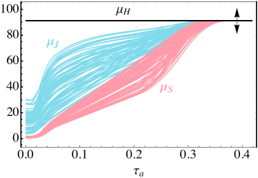
$a=0$
$a=0.5$

Figure 10: Profile functions implemented in our resummation, shown for $a=\{-1.0,-0.5,0.0,0.5\}$ and $Q=m_{Z}$. Left: Band method. Right: Scan method. Each set of profiles $\mu_{H,J,S}$ actually has a different absolute vertical scale set by $\mu_{H}=e_{H}Q$, which has been rescaled for this illustration to $e_{H}=1$. Also, for each individual set of scales, it is the case that $\mu_{S}<\mu_{J}$, although the overall bands from the scan overlap.

In the left panel of Fig. 10, we illustrate the width of the jet- and soft-scale variations for $a=\{-1.0,\,-0.5,\,0.0,\,0.5\}$ and $Q=m_{Z}$. One clearly observes the leveling off in the low $\tau_{a}$ region, the natural behavior in the mid $\tau_{a}$ region, and finally the convergence of all three scales in the far-tail region. Again, the coloured bands represent independent variations of the jet and soft scales through $e_{J,S}\in\{-0.5,0.0,0.5\}$. The third hard-scale variation then corresponds to shifting the overall scale of the plots in Fig. 10 up and down, and we do so through $Q/2\leq\mu_{H}\leq 2Q$.

The last three variations are not illustrated in Fig. 10. The nonsingular scale variation is designed to probe missing fixed-order terms not accounted for in our calculation, and the variation of $c_{\tilde{J}}^{2}$ and $r^{2}$ estimate the systematic uncertainty of our EVENT2 extraction of both the two-loop jet-function constant and the $\mathcal{O}(\alpha_{s}^{2})$ remainder function. For the former, differences from central values are obtained by maximizing and minimizing the cross section over the listed uncertainties of $c_{\tilde{J}}^{2}$ in Table 4. For the latter, differences from central values are obtained by varying $r^{2}(\tau_{a})$ across the 1-$\sigma$ error bands obtained in the NonLinearModelFit described in Section 3.3 (these procedures correspond to setting the parameters $\delta c^{2}_{\tilde{J}}$ and $\delta r^{2}$ to $\pm 1$ in Eqs. (125) and (126) below). The errors induced by these variations are minimal in comparison to the other four variations.

Scan method

For the scan method we take 64 random selections of profile and scale parameters within the ranges shown in Table 7. Note that in this method we have chosen not to vary $e_{S}$ away from 0, thus allowing the variations of the other relevant parameters (e.g. $n_{0},n_{1},\mu_{0},r$) to probe the relevant range of the soft scale $\mu_{S}$. Note also that we fix $R_{0}$ to always be ($\mu_{0}-0.4$ GeV) so that while $\mu_{0}$ varies, the difference between $\mu_{0}$ and $R_{0}$ remains fixed, to preserve the scheme choice for the gap parameter $\Delta_{a}$ (cf. Abbate:2010xh ; Hoang:2014wka ). The parameters $\delta c_{\tilde{J}}^{2}$ and $\delta r^{2}$ are defined to probe the uncertainties coming from scanning over the 1-$\sigma$ ranges of $c_{\tilde{J}}^{2}$ and $r^{2}(\tau_{a})$ determined in Sec. 3. That is, we take

$$c_{\tilde{J}}^{2}=c_{\tilde{J}}^{2,\text{central}}+\begin{cases}\delta c_{\tilde{J}}^{2}\;\Delta c_{\tilde{J}}^{2,\text{upper}}&\delta c_{\tilde{J}}^{2}>0\\ \delta c_{\tilde{J}}^{2}\;\Delta c_{\tilde{J}}^{2,\text{lower}}&\delta c_{\tilde{J}}^{2}<0\end{cases}\,,$$ (125)

where “central, upper, lower” refer to the central values, upper, and lower uncertainties on $c_{\tilde{J}}^{2}$ given in Table 4. Similarly,

$$r^{2}(\tau_{a})=r^{2,\text{central}}(\tau_{a})+\delta r^{2}\;\Delta r^{2}(\tau_{a})\,,$$ (126)

where $r^{2,\text{central}}$ and $\Delta r^{2}$ are the central values and 1-$\sigma$ uncertainty function illustrated in Fig. 8.

In the right panel of Fig. 10, we show the analogous width of the jet- and soft-scale variations probed with the scan method. As is clear, the error bands between the two methods are of a similar form and they exhibit all of the qualities we demand of the profile functions across the whole $\tau_{a}$ domain. Given the current scan ranges and parameter choices, the errors in the scan method indeed appear to be larger than those of the band method, but this is somewhat compensated for by taking the simple envelope of resulting variations rather than adding in quadrature. In the next section we will apply both methods to our final predictions for the resummed and matched cross sections, and we will compare the quality of their convergence both for integrated and differential distributions.

6 Results and data comparison

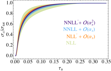
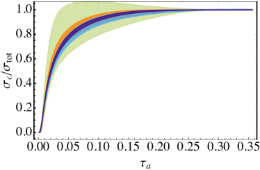
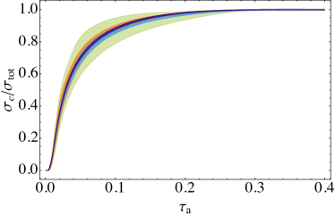
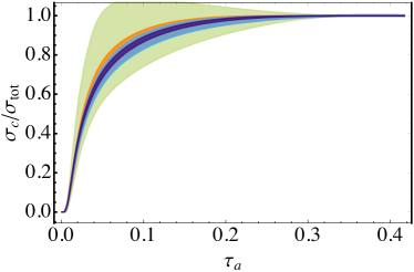
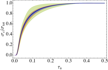
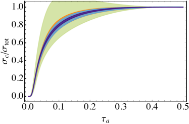
Band Method                                 Scan Method
$a=-1$ $a=-0.5$ $a=0$ $a=0.5$

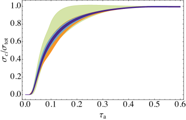
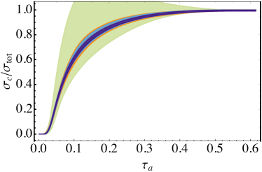
Figure 11: Integrated angularity distributions for four values of $a=\{-1.0,-0.5,0.0,0.5\}$ and $Q=m_{Z}$ at NLL (green), NLL${}^{\prime}+\mathcal{O}(\alpha_{s})$ (orange), NNLL$+\mathcal{O}(\alpha_{s})$ (blue), and NNLL${}^{\prime}+\mathcal{O}(\alpha_{s}^{2})$ (purple) accuracy, with renormalon subtractions to the corresponding orders. The theoretical uncertainties have been estimated with the band method (left) and the scan method (right) as discussed in Sec. 5.2.

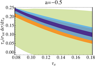
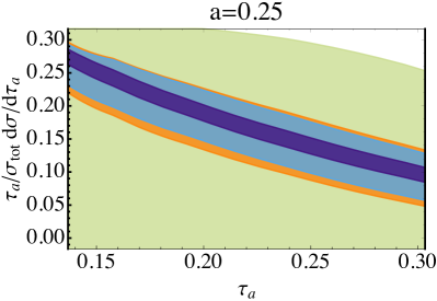
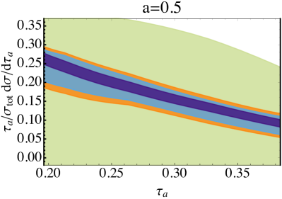
Figure 12: Differential angularity distributions for four values of $a=\{-0.5,-0.25,0.25,0.5\}$ and $Q=m_{Z}$ in the central $\tau_{a}$ region, resummed and matched to NLL (green), NLL${}^{\prime}+\mathcal{O}(\alpha_{s})$ (orange), NNLL$+\mathcal{O}(\alpha_{s})$ (blue), and NNLL${}^{\prime}+\mathcal{O}(\alpha_{s}^{2})$ (purple) accuracy, with renormalon subtractions to the corresponding orders, and uncertainties estimated with the scan method.

We now present our predictions for the angularity distributions for seven values of the angularity parameter $a\in\{-1.0,\,-0.75,\,-0.5,\,-0.25,\,0.0,\,0.25,\,0.5\}$ at $Q=91.2$ GeV and $Q=197$ GeV, and compare them to the L3 data presented in Achard:2011zz . In our analysis we will use the $\overline{\mathrm{MS}}$ coupling constant $\alpha_{s}(m_{Z})=0.11$ and the non-perturbative shift parameter, defined through Eq. (103), $\Omega_{1}(R_{\Delta},R_{\Delta})=0.4$ GeV at $R_{\Delta}=1.5$ GeV. These values are chosen to be consistent with the central fit values from Hoang:2015hka for $\alpha_{s}(m_{Z})$ (to two signficant digits) and $\Omega_{1}(R_{\Delta},R_{\Delta})$ (to one signficant digit) at NNLL^′ accuracy. Some discussion on the phenomenological impact of choosing different values for these input parameters will be given in Sec. 7.

We first show in Fig. 11 our predictions for the integrated distributions $\sigma_{c}(\tau_{a})$ given by Eqs. (112) and (113) for four values of $a$ at $Q=m_{Z}$ up to NNLL${}^{\prime}+\mathcal{O}(\alpha_{s}^{2})$ accuracy, including renormalon subtractions. At the same time we compare the two methods discussed in Sec. 5.2 to estimate the overall uncertainties of our analysis. The band method has been applied in the left panel and the scan method in the right panel. One clearly observes that moving to primed accuracies not only dramatically reduces the scale uncertainties, but that also the variations converge across the entire spectra as we move to higher accuracies. One also sees that the two methods that have been applied to estimate the theory uncertainties are consistent with one another, given the parameter ranges and variations chosen. However, when computing differential distributions by taking the derivative of Eq. (112), we notice a slight improvement in numerical stability when using the scan method. This is partially due to the envelope of the many (64) variations smoothing out wiggles coming from derivatives of profile functions $\mu_{i}(\tau_{a})$, especially in transition regions. Fig. 12 illustrates this convergence of the differential distribution (multiplied by $\tau_{a}$) in the central $\tau_{a}$ domain for four values of the angularity parameter $a$. For this reason, and to allow for a more direct comparison of our results to those of Abbate:2010xh ; Hoang:2014wka ; Hoang:2015hka , we implement theory uncertainties as obtained with the scan method in the following.

$a=-0.5$
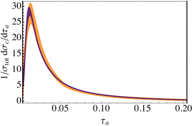
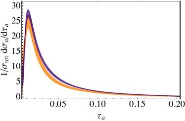
$a=0.25$

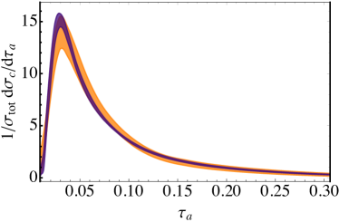
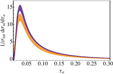
Figure 13: Differential angularity distributions for $a=-0.5$ and $a=0.25$ at $Q=m_{Z}$ over the entire $\tau_{a}$ domain. The distributions correspond to NLL${}^{\prime}+\mathcal{O}(\alpha_{s})$ (orange) and NNLL${}^{\prime}+\mathcal{O}(\alpha^{2}_{s})$ (purple) accuracy with renormalon subtractions, and they are either obtained as the derivative of the integrated distributions (left) or directly resummed as differential distributions (right). As expected from the analysis in Almeida:2014uva , the former show a bit better convergence than the latter.

In order to demonstrate the improvement in precision that we achieve for the differential distributions in moving from NLL${}^{\prime}+\mathcal{O}(\alpha_{s})$ Hornig:2009vb to NNLL${}^{\prime}+\mathcal{O}(\alpha^{2}_{s})$ accuracy, we present our (renormalon-subtracted) predictions for $a=\{-0.5,0.25\}$ and $Q=m_{Z}$ across the entire $\tau_{a}$ domain in Fig. 13. This figure also illustrates the differences between taking the derivative of the integrated distributions (which we call $d\sigma_{c}/d\tau_{a}$ here) in the left panel, and directly evaluating the resummed (“naïve”) differential distributions (which we call $d\sigma_{n}/d\tau_{a}$ here) in the right panel. We see that the former give better convergence and that they better preserve the total integral under the distributions. These issues with the naïve distributions were extensively discussed in Almeida:2014uva . In fact, as shown there, at unprimed orders the naïve formulas do not even preserve the correct order of accuracy, and even the primed orders suffer from the illustrated mismatch with the total integral under the curve. These issues can be remedied by supplementing the naïve formula with additional terms that both preserve accuracy (at unprimed orders) and maintain agreement with the total integral under the curve (at any order). See Almeida:2014uva ; Procura:2018zpn for such strategies, and Bertolini:2017eui for a beautiful mathematical solution to this problem. Here, for simplicity, we have not implemented such strategies, and we simply stick to the integrated distributions from Eq. (112) as the basis for all of our predictions.

	Slope $r_{s}=1/\tau_{a}^{\text{sph}}$	Slope $r_{s}=1$
$a=-0.5$
$a=0.25$

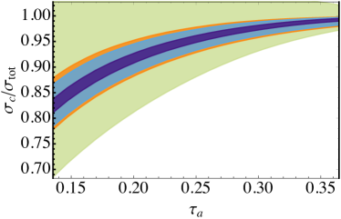
Figure 14: Integrated angularity distributions for $a=-0.5$ and $a=0.25$ at $Q=m_{Z}$ at NLL (green), NLL${}^{\prime}+\mathcal{O}(\alpha_{s})$ (orange), NNLL$+\mathcal{O}(\alpha_{s})$ (blue), and NNLL${}^{\prime}+\mathcal{O}(\alpha_{s}^{2})$ (purple) accuracy, with renormalon subtractions to the corresponding orders. The distributions have been obtained with the slope parameter $r_{s}=1/\tau_{a}^{\text{sph}}$ (left) and $r_{s}=1$ (right).

In Fig. 14 we illustrate the effect of choosing a slope parameter $r_{s}=1/\tau_{a}^{\text{sph}}$ for the running scale in Eq. (117) in the resummation region. In this figure we compare predictions for integrated distribution for $a=\{-0.5,0.25\}$ and $Q=m_{Z}$ at different logarithmic accuracies. One observes that the convergence is slightly better for the choice $r_{s}=1/\tau_{a}^{\text{sph}}$ than for $r_{s}=1$, although the differences between both choices become smaller at higher logarithmic accuracies. This is consistent with the findings of Hoang:2014wka , who made a similar comparison for thrust ($a=0$), and this also validates our interpretation of the slope parameter $r_{s}$ as being related to the maximum value of the angularity $\tau_{a}^{\text{sph}}$.

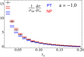
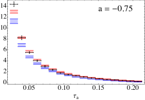
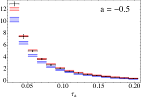
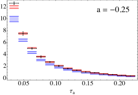
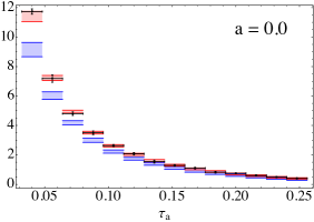
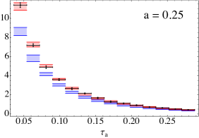
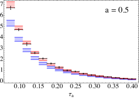
Figure 15: NNLL^′ resummed and $\mathcal{O}(\alpha_{s}^{2})$ matched angularity distributions for all values of $a$ considered in this study, $a\in\{-1.0,-0.75,-0.5,-0.25,0.0,0.25,0.5\}$, at $Q=m_{Z}$, with $\alpha_{s}(m_{Z})=0.11$. The blue bins represent the purely perturbative prediction and the red bins include a convolution with a gapped and renormalon-subtracted shape function, with a first moment set to $\Omega_{1}(R_{\Delta},R_{\Delta})=0.4\text{ GeV}$. Overlaid is the experimental data from Achard:2011zz .

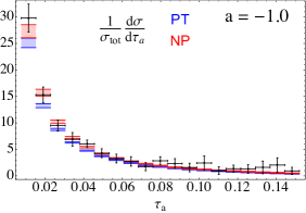
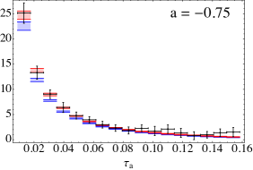
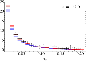
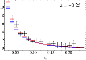
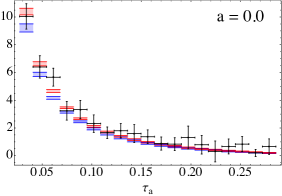
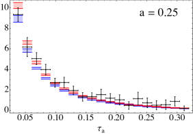
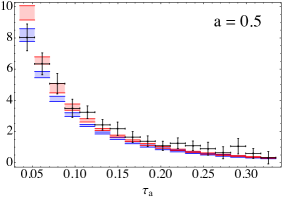
Figure 16: The same as in Figure 15, but with $Q=197$ GeV.

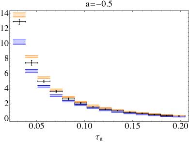
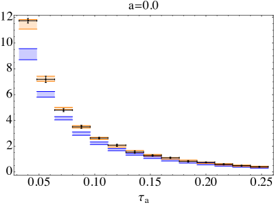
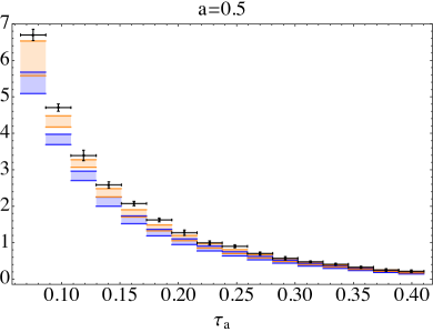
Figure 17: The same as in Figure 15 (for $a=\{-1.0,-0.5,0.0,0.5\}$), but with the non-perturbative scaling coefficient purposefully altered to $c_{\tau_{a}}=2.0$, instead of $c_{\tau_{a}}=2/(1-a)$.

Finally, we present binned results for NNLL^′ resummed, $\mathcal{O}(\alpha_{s}^{2})$ matched and renormalon-subtracted differential distributions for $a=\{-1.0,-0.75,-0.5,-0.25,0.0,0.25,0.5\}$ in Fig. 15 ($Q=m_{Z}$) and Fig. 16 ($Q=197$ GeV). To obtain the binning, we have integrated the upper and lower bounds of the differentiated cumulative distribution over each bin, which we then divided by the bin width. In both cases we compare to the data from the L3 collaboration Achard:2011zz , and we explicitly illustrate the effect of including the non-perturbative effects from Eq. (113) (red bins). In the figures we focus on the central $\tau_{a}$ domain where the effect of the resummation is most relevant. It is clear that—given the parameters we have applied in our analysis—the data is consistent with the non-perturbative shifted curves for the entirety of the angularity spectra. On the other hand, the bins obtained using only the perturbative predictions (blue bins) systematically undershoot the available data throughout the resummation-sensitive region. These observations are less obvious with the less precise 197 GeV data in Fig. 16, which nevertheless provides a decent test of the $Q$ dependence of $\alpha_{s}$ and the $1/Q$ scaling of the leading nonperturbative correction.

These results serve as an impressive visual confirmation of the leading non-perturbative correction discussed in Sec. 4, which clearly indicates a scaling with the angularity parameter $a$. To further emphasize that this scaling is actually reflected in the data, in Fig. 17 we have drawn analogous plots to those in Fig. 15, but we have purposefully altered the non-perturbative scaling coefficient such that $c_{\tau_{a}}\rightarrow 2.0$, instead of the predicted $c_{\tau_{a}}=2/(1-a)$. The associated bins for the predictions convolved with a renormalon-free shape function, now shown in orange, clearly overshoot the data at $a=\{-1.0,-0.5\}$, obviously remain unchanged for thrust ($a=0$), and are beginning to slightly undershoot some bins at $a=0.5$. This indicates that the scaling $c_{\tau_{a}}=2/(1-a)$ is indeed a good theoretical prediction.

Note that the leading bin depicted in all panels of Figs. 15–17 is actually the first bin after the peak of the distribution, as determined by the experimental data. It is unsurprising that in most cases our theory predictions do not successfully describe this data point, as it is particularly sensitive to the form of the non-perturbative shape function. As described in Sec. 4.1, we have only included the first term in its expansion in a series of basis functions, and one would need to include additional terms in this expansion in order to accurately describe the data in the peak region.

The above results serve as a powerful visual confirmation of the predictions of factorization and resummation in QCD using the SCET framework, the evolution of $\alpha_{s}$, and the scaling and universality of leading non-perturbative corrections for $e^{+}e^{-}$ event shapes. We have not yet performed a full, robust statistical fit to the available L3 data for $\alpha_{s}(m_{Z})$ and $\Omega_{1}(R_{\Delta},R_{\Delta})$, but visually the fit values from Hoang:2015hka appear consistent within our calculations when compared to the data in Fig. 15. This motivates carrying out such a fit to the available LEP angularity data in the future.

7 Summary and outlook

We have presented NNLL^′ resummed and $\mathcal{O}(\alpha_{s}^{2})$ matched distributions for the $e^{+}e^{-}$ event shape angularities at $Q=91.2$ GeV and $Q=197$ GeV. Our results are the most precise achieved for this observable to date, and they are made possible by a recent calculation of the two-loop soft anomalous dimension $\gamma_{S}^{1}$ Bell:2015lsf ; Bell:2018vaa and finite constants $c_{\tilde{S}}^{2}$ Bell:2015lsf ; Bell:2018oqa . We determined the remaining unknown NNLL^′ ingredient $c_{\tilde{J}}^{2}$ from a fit to the EVENT2 generator, from which we also obtained the fixed-order matching to QCD at $\mathcal{O}(\alpha_{s}^{2})$. We further modeled non-perturbative effects with a gapped shape function whose renormalon ambiguity was cancelled using the “Rgap” scheme to define the appropriate subtractions and obtain the “$R$-evolution” of the non-perturbative moment $\Omega_{1}(\mu,R)$. Finally, reliable theory uncertainty estimates have been obtained via variations about a suitable profile function describing the transition of non-perturbative and perturbative scales throughout the relevant domain.

We have compared the predictions resulting from this analysis to data from the L3 collaboration, and find excellent agreement for all angularities considered in this study. In particular, we have visually confirmed the predicted sensitivity of the distributions to leading non-perturbative scaling effects that are simultaneously encoded in the angularity parameter $a$ and the universal shift parameter ${\Omega}_{1}$ — the distributions indeed seem to require shifts proportional to $2/(1-a)$ in order to accurately describe the data.

$a=-1.0$	$a=0.5$

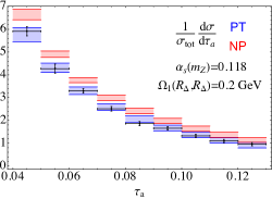
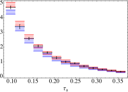
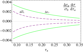
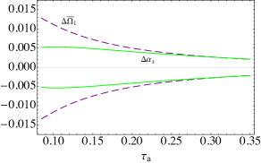
Figure 18: Top: A binned data comparison at $a=\{-1.0,\,0.5\}$ for distributions generated with $\alpha_{s}(m_{Z})=0.118$ and $\Omega_{1}(R_{\Delta},R_{\Delta})=0.2$ GeV. All other settings are the same as in Figure 15. As is clear, the final renormalon-corrected (red) curves overshoot the data at $a=-1.0$ but, thanks to the small shift parameter, successfully describe the $a=0.5$ data. Bottom: Difference between central curves and curves evaluated with single variations of either $\overline{\Omega}_{1}$ (dashed, purple) or $\alpha_{s}(m_{Z})$ (solid, green) at the same values of $a$ and $Q=m_{Z}$. Note that the lower plots are generated with canonical scales, are unmatched, and the variation about $\overline{\Omega}_{1}$ is illustrated using the shift (3), rather than the fully shape and renormalon-corrected formulae.

This characteristic non-perturbative scaling strongly motivates an extraction of both $\alpha_{s}$ and $\Omega_{1}$ from a fit to experimental data on angularities. As previous extractions of $\alpha_{s}$ from $e^{+}e^{-}$ event shapes like thrust and $C$-parameter have shown Abbate:2010xh ; Abbate:2012jh ; Hoang:2015hka , the disentangling of perturbative and non-perturbative effects is crucial and has a large impact on the determined value of $\alpha_{s}$ itself. Thus angularities, with their tunable relative contributions of these effects, can play an important role in confirming (or not) the values coming from these other extractions, which as mentioned before, are considerably lower than the PDG world average PhysRevD.98.030001 . While we have not performed a dedicated extraction in this study, in the top panels of Fig. 18 we have shown the analogous plots to those in Fig. 15 at $a=\{-1.0,0.5\}$, but with $\alpha_{s}(m_{Z})=0.118$ (consistent with the PDG value) and $\Omega_{1}(R_{\Delta},R_{\Delta})=0.2$ GeV, just large enough to consistently implement our gap parameter and provide a good fit to the data for the angularity $a=0.5$. As can be seen, however, at $a=-1.0$ the final theory bins are then well above the data in the tail region. As the practical effect of lowering (raising) $\alpha_{s}(m_{Z})$ (${\Omega}_{1}$) away from the best values used in Fig. 15 is to the lower (raise) the theory prediction, this naïve exercise leads one to provisionally expect that such parameter values will be difficult to reconcile with the available data.

In the bottom panels of Fig. 18 we finally show the difference $(d\sigma/d\tau_{a})_{\text{central}}-d\sigma/d\tau_{a}$ over the range $0.085\leq\tau_{a}\leq 0.35$ for $a=\{-1.0,\,0.5\}$, where $(d\sigma/d\tau_{a})_{\text{central}}$ is an (unmatched, non-renormalon corrected) NNLL^′ resummed curve. For $(d\sigma/d\tau_{a})$ we have varied 2$\overline{\Omega}_{1}$ by $\pm\,0.1$ GeV and $\alpha_{s}(m_{Z})$ by $\pm\,0.001$, corresponding to the purple and green curves, respectively. Our plots are to be compared to Fig. 10 in Abbate:2010xh , where the same variations were made at different center-of-mass energies $Q$. We find that varying $a$ ($Q$) down (up) from high (low) values leads to an enhanced sensitivity to the relative effects of $\alpha_{s}$ and $\overline{\Omega}_{1}$ variation. This suggests that extractions from angularity data at a single centre-of-mass energy $Q$, but different values of $a$, will be able to discriminate between $\alpha_{s}$ and $\overline{\Omega}_{1}$ in a similar way to varying $Q$. In fact, angularities for $-2\leq a\leq 0.5$ exhibit a factor of six variance in the overall non-perturbative shift, which represents an essentially equivalent sensitivity to measurements made between $Q=35$ GeV and $Q=207$ GeV, as analyzed for thrust in Abbate:2010xh . Unfortunately, angularity data is currently only available down to $a=-1.0$ and only at two values of $Q$. Thus a reanalysis of additional LEP data would be highly desirable. Of course, a high-precision determination of $\alpha_{s}$ and $\Omega_{1}$ should ideally also include further theory improvements beyond those we have already implemented here, such as hadron mass effects or higher-precision numerical (or even analytical) determinations of $c_{\tilde{J}}^{2}$ and $r^{2}(\tau_{a})$. New methods and calculations for $\mathcal{O}(\alpha_{s}^{3})$ jet and soft functions at $a\neq 0$ would be needed to go to N³LL$(^{\prime})$ accuracy, while $\mathcal{O}(\alpha_{s}^{3})$ fixed-order matching to QCD could be obtained from a program like EERAD3 Ridder:2014wza . In conclusion, we are optimistic that the $a$-dependence of the angularities may ultimately be helpful in lifting degeneracies between $\alpha_{s}$ and ${\Omega}_{1}$ in the two-parameter event-shape fits. We leave it to future work to bring such an analysis to full culmination.

Appendix A Laplace transforms

In this appendix we collect results for the Laplace transforms and inverse Laplace transforms between the logarithms

$$L\equiv\ln\frac{1}{\tau}\,,\qquad\tilde{L}\equiv\ln(\nu e^{\gamma_{E}})\,.$$ (127)

The Laplace transforms, defined by

$$\widetilde{F}(\nu)\equiv\mathscr{L}\{F\}(\nu)=\int_{0}^{\infty}d\tau\,e^{-\nu\tau}F(\tau)$$ (128)

are given by

$$\mathscr{L}\bigl{\{}1\bigr{\}} =\frac{1}{\nu}\,, \mathscr{L}\bigl{\{}L^{3}\bigr{\}} =\frac{1}{\nu}\biggl{\{}\tilde{L}^{3}+\frac{\pi^{2}}{2}\tilde{L}+2\zeta_{3}\biggr{\}}\,,$$ (129)

$$\mathscr{L}\bigl{\{}L\bigr{\}} =\frac{1}{\nu}\,\tilde{L}\,, \mathscr{L}\bigl{\{}L^{4}\bigr{\}} =\frac{1}{\nu}\biggl{\{}\tilde{L}^{4}+\pi^{2}\tilde{L}^{2}+8\zeta_{3}\tilde{L}+\frac{3\pi^{4}}{20}\biggr{\}}\,,$$

$$\mathscr{L}\bigl{\{}L^{2}\bigr{\}} =\frac{1}{\nu}\biggl{\{}\tilde{L}^{2}+\frac{\pi^{2}}{6}\biggr{\}}\,,$$

and so on. The inverse Laplace transforms, defined by

$$\mathscr{L}^{-1}\{\widetilde{F}\}(\tau)=\int_{\gamma-i\infty}^{\gamma+i\infty}\,\frac{d\nu}{2\pi i}\,e^{\nu\tau}\widetilde{F}(\nu)\,,$$ (130)

where $\gamma$ lies to the right of all the poles of $\widetilde{F}$ in the complex plane, are given by

$$\mathscr{L}^{-1}\Bigl{\{}\frac{1}{\nu}\Bigr{\}} =1\,, \mathscr{L}^{-1}\Bigl{\{}\frac{1}{\nu}\tilde{L}^{3}\Bigr{\}} =L^{3}-\frac{\pi^{2}}{2}L-2\zeta_{3}\,,$$ (131)

$$\mathscr{L}^{-1}\Bigl{\{}\frac{1}{\nu}\tilde{L}\Bigr{\}} =L\,, \mathscr{L}^{-1}\Bigl{\{}\frac{1}{\nu}\tilde{L}^{4}\Bigr{\}} =L^{4}-\pi^{2}L^{2}-8\zeta_{3}L+\frac{\pi^{4}}{60}\,,$$

$$\mathscr{L}^{-1}\Bigl{\{}\frac{1}{\nu}\tilde{L}^{2}\Bigr{\}} =L^{2}-\frac{\pi^{2}}{6}\,,$$

and so on. The results explicitly tabulated in Eqs. (129) and (131) are needed to transform logarithms in the fixed-order expansions of event-shape distributions in QCD up to $\mathcal{O}(\alpha_{s}^{2})$.

Appendix B Anomalous dimensions

The coefficients of the beta function up to four-loop order in the $\overline{\mathrm{MS}}$ scheme are given by Tarasov:1980au ; Larin:1993tp ; vanRitbergen:1997va

$$\beta_{0} =\frac{11}{3}\,C_{A}-\frac{4}{3}\,T_{F}\,n_{f}\,,$$ (132)

$$\beta_{1} =\frac{34}{3}\,C_{A}^{2}-\Bigl{(}\frac{20}{3}\,C_{A}\,+4C_{F}\Bigr{)}\,T_{F}\,n_{f}\,,$$

$$\beta_{2} =\frac{2857}{54}\,C_{A}^{3}+\Bigl{(}C_{F}^{2}-\frac{205}{18}\,C_{F}C_{A}-\frac{1415}{54}\,C_{A}^{2}\Bigr{)}\,2T_{F}\,n_{f}+\Bigl{(}\frac{11}{9}\,C_{F}+\frac{79}{54}\,C_{A}\Bigr{)}\,4T_{F}^{2}\,n_{f}^{2}\,,$$

$$\beta_{3} =4826.16\quad(N_{C}=3,n_{f}=5)\,.$$ (133)

The running coupling $\alpha_{s}(\mu)$ up to four-loop accuracy is given by the formula,

$$\frac{\alpha_{s}(m_{Z})}{\alpha_{s}(\mu)}=X+\frac{\alpha_{s}(m_{Z})}{4\pi}\frac{\beta_{1}}{\beta_{0}}\ln X+\Bigl{(}\frac{\alpha_{s}(m_{Z})}{4\pi}\Bigr{)}^{2}\biggl{[}\frac{\beta_{2}}{\beta_{0}}\Bigl{(}1\!-\!\frac{1}{X}\Bigr{)}+\frac{\beta_{1}^{2}}{\beta_{0}^{2}}\Bigl{(}\frac{\ln X}{X}\!+\!\frac{1}{X}\!-\!1\Bigr{)}\biggr{]}$$ (134)

$$+\Bigl{(}\frac{\alpha_{s}(m_{Z})}{4\pi}\Bigr{)}^{3}\frac{1}{X^{2}}\biggl{[}\frac{\beta_{3}}{2\beta_{0}}(X^{2}\!-\!1)+\frac{\beta_{1}\beta_{2}}{\beta_{0}^{2}}(X\!+\!\ln X\!-\!X^{2})+\frac{\beta_{1}^{3}}{2\beta_{0}^{3}}\bigl{(}(1\!-\!X)^{2}\!-\!\ln^{2}X\bigr{)}\biggr{]}\,,$$

where

$$X\equiv 1+\frac{\alpha_{s}(m_{Z})\beta_{0}}{2\pi}\ln\frac{\mu}{m_{Z}}\,.$$ (135)

The four-loop term in Eq. (134) agrees with the numerical form given in Abbate:2010xh , and is rederived below in App. C.

The cusp anomalous dimension coefficients are given up to 3-loop order  Korchemsky:1987wg ; Moch:2004pa

$$\Gamma^{q}_{0} =4C_{F}\,,$$ (136)

$$\Gamma^{q}_{1} =4C_{F}\Bigl{[}\Bigl{(}\frac{67}{9}-\frac{\pi^{2}}{3}\Bigr{)}\,C_{A}-\frac{20}{9}\,T_{F}\,n_{f}\Bigr{]}\,,$$

$$\Gamma^{q}_{2} =4C_{F}\Bigl{[}\Bigl{(}\frac{245}{6}-\frac{134\pi^{2}}{27}+\frac{11\pi^{4}}{45}+\frac{22\zeta_{3}}{3}\Bigr{)}C_{A}^{2}+\Bigl{(}-\frac{418}{27}+\frac{40\pi^{2}}{27}-\frac{56\zeta_{3}}{3}\Bigr{)}C_{A}\,T_{F}\,n_{f}$$

$$\hskip 34.44434pt+\Bigl{(}-\frac{55}{3}+16\zeta_{3}\Bigr{)}C_{F}\,T_{F}\,n_{f}-\frac{16}{27}\,T_{F}^{2}\,n_{f}^{2}\Bigr{]}\,.$$

The $\overline{\mathrm{MS}}$ non-cusp anomalous dimension for the hard function can be obtained Idilbi:2006dg ; Becher:2006mr from the infrared divergences of the on-shell massless quark form factor, which are known to three loops Moch:2005id ,

$$\gamma_{H}^{0} =-12C_{F}\,,$$ (137)

$$\gamma_{H}^{1} =-2C_{F}\Bigl{[}\Bigl{(}\frac{82}{9}-52\zeta_{3}\Bigr{)}C_{A}+(3-4\pi^{2}+48\zeta_{3})C_{F}+\Bigl{(}\frac{65}{9}+\pi^{2}\Bigr{)}\beta_{0}\Bigr{]}\,,$$

$$\gamma_{H}^{2} =-4C_{F}\Bigl{[}\Bigl{(}\frac{66167}{324}-\frac{686\pi^{2}}{81}-\frac{302\pi^{4}}{135}-\frac{782\zeta_{3}}{9}+\frac{44\pi^{2}\zeta_{3}}{9}+136\zeta_{5}\Bigr{)}C_{A}^{2}$$

$$\quad+\Bigl{(}\frac{151}{4}-\frac{205\pi^{2}}{9}-\frac{247\pi^{4}}{135}+\frac{844\zeta_{3}}{3}+\frac{8\pi^{2}\zeta_{3}}{3}+120\zeta_{5}\Bigr{)}C_{F}C_{A}$$

$$\quad+\Bigl{(}\frac{29}{2}+3\pi^{2}+\frac{8\pi^{4}}{5}+68\zeta_{3}-\frac{16\pi^{2}\zeta_{3}}{3}-240\zeta_{5}\Bigr{)}C_{F}^{2}$$

$$\quad+\Bigl{(}-\frac{10781}{108}+\frac{446\pi^{2}}{81}+\frac{449\pi^{4}}{270}-\frac{1166\zeta_{3}}{9}\Bigr{)}C_{A}\beta_{0}$$

$$\quad+\Bigl{(}\frac{2953}{108}-\frac{13\pi^{2}}{18}-\frac{7\pi^{4}}{27}+\frac{128\zeta_{3}}{9}\Bigr{)}\beta_{1}+\Bigl{(}-\frac{2417}{324}+\frac{5\pi^{2}}{6}+\frac{2\zeta_{3}}{3}\Bigr{)}\beta_{0}^{2}\Bigr{]}\,.$$

In the text we found it convenient to split up the Abelian and non-Abelian pieces of $\gamma_{H}^{1}$. We define

$$\begin{split}\gamma_{H}^{1}\bigr{\rvert}_{C_{F}}&\equiv-2C_{F}^{2}(3-4\pi^{2}+48\zeta_{3})\,,\\ \gamma_{H}^{1}\bigr{\rvert}_{\text{n.A.}}&\equiv-2C_{F}\biggl{[}\biggl{(}\frac{82}{9}-52\zeta_{3}\biggr{)}C_{A}+\biggl{(}\frac{65}{9}+\pi^{2}\biggr{)}\beta_{0}\biggr{]}\,.\end{split}$$ (138)

The non-cusp anomalous dimensions for the $a=0$ soft function are given explicitly by

$$\gamma_{S}^{0} =0\,,$$ (139)

$$\gamma_{S}^{1} =-2C_{F}\Bigl{[}\Big{(}\frac{64}{9}-28\zeta_{3}\Bigr{)}C_{A}+\Bigl{(}\frac{56}{9}-\frac{\pi^{2}}{3}\Bigr{)}\beta_{0}\Bigr{]}\,,$$

$$\gamma_{S}^{2} =-2C_{F}\bigg{[}C_{A}^{2}\bigg{(}\frac{37871}{162}-\frac{310\pi^{2}}{81}-\frac{8\pi^{4}}{5}-\frac{2548\zeta_{3}}{9}+\frac{88\pi^{2}\zeta_{3}}{9}+192\zeta_{5}\bigg{)}$$

$$\qquad\quad+C_{A}\beta_{0}\bigg{(}-\frac{4697}{54}-\frac{242\pi^{2}}{81}+\frac{56\pi^{4}}{45}-\frac{220\zeta_{3}}{9}\bigg{)}$$

$$\qquad\quad+\beta_{1}\bigg{(}\frac{1711}{54}-\frac{\pi^{2}}{3}-\frac{4\pi^{4}}{45}-\frac{152\zeta_{3}}{9}\bigg{)}+\beta_{0}^{2}\bigg{(}-\frac{520}{81}-\frac{5\pi^{2}}{9}+\frac{28\zeta_{3}}{3}\bigg{)}\bigg{]}\,.$$

For $a\neq 0$, we have $\gamma_{S}^{0}(a)=0$ Hornig:2009vb and the non-cusp two-loop soft anomalous dimension was given in Eq. (38). The non-cusp jet anomalous dimension is then given by the consistency relation $2\gamma_{J}=-\gamma_{H}-\gamma_{S}$.

Appendix C RG invariance of total evolution kernels

C.1 Residual scale dependence due to standard change of variables

Renormalization group (RG) invariance of the physical cross section guarantees that the combination of all evolution kernels on the right-hand side of Eq. (2.1) is independent of the scale $\mu$. This is in fact true not only in the limit of infinite accuracy in perturbation theory in $\alpha_{s}$, but at each finite order of resummed and fixed-order accuracy, as a consequence of the anomalous dimensions satisfying the consistency relation $\gamma_{H}(\mu)+2\gamma_{J}(\mu)+\gamma_{S}(\mu)=0$ at each finite order. The evaluation of $K_{\Gamma}$ defined in Eq. (13), after the change of integration variables Eq. (27),

$$K_{\Gamma}(\mu,\mu_{F})=\int_{\alpha_{s}(\mu_{F})}^{\alpha_{s}(\mu)}\frac{d\alpha}{\beta[\alpha]}\Gamma_{\rm cusp}[\alpha]\int_{\alpha_{s}(\mu_{F})}^{\alpha}\frac{d\alpha^{\prime}}{\beta[\alpha^{\prime}]}\,,$$ (140)

order-by-order in logarithmic accuracy gives the well-known results (e.g. Ligeti:2008ac ; Abbate:2010xh ):

$$K_{\Gamma}^{\text{LL}}(\mu,\mu_{F}) =\frac{\Gamma_{0}}{4\beta_{0}^{2}}\frac{4\pi}{\alpha_{s}(\mu_{F})}\biggl{\{}\ln r+\frac{1}{r}-1\biggr{\}}\,,$$ (141a)

$$K_{\Gamma}^{\text{NLL}}(\mu,\mu_{F}) =\frac{\Gamma_{0}}{4\beta_{0}^{2}}\biggl{\{}\left(\frac{\Gamma_{1}}{\Gamma_{0}}\!-\!\frac{\beta_{1}}{\beta_{0}}\right)(r\!-\!1\!-\!\ln r)\!-\!\frac{\beta_{1}}{2\beta_{0}}\ln^{2}r\biggr{\}}\,,$$ (141b)

$$K_{\Gamma}^{\text{NNLL}}(\mu,\mu_{F}) =\frac{\Gamma_{0}}{4\beta_{0}^{2}}\frac{\alpha_{s}(\mu_{F})}{4\pi}\biggl{\{}B_{2}\left(\frac{r^{2}\!-\!1}{2}-\ln r\right)+\left(\frac{\beta_{1}\Gamma_{1}}{\beta_{0}\Gamma_{0}}\!-\!\frac{\beta_{1}^{2}}{\beta_{0}^{2}}\right)(r\!-\!1\!-\!r\ln r)$$ (141c)

$$\qquad\qquad\qquad+\left(\frac{\Gamma_{2}}{\Gamma_{0}}-\frac{\beta_{1}\Gamma_{1}}{\beta_{0}\Gamma_{0}}\right)\frac{(1-r)^{2}}{2}\biggr{\}}\,,$$

$$K_{\Gamma}^{\text{N${}^{3}$LL}}(\mu,\mu_{F}) =\frac{\Gamma_{0}}{4\beta_{0}^{2}}\Bigl{(}\frac{\alpha_{s}(\mu_{F})}{4\pi}\Bigr{)}^{2}\biggl{\{}\Bigl{(}\frac{\Gamma_{3}}{\Gamma_{0}}-\frac{\Gamma_{2}\beta_{1}}{\Gamma_{0}\beta_{0}}+\frac{\Gamma_{1}}{\Gamma_{0}}B_{2}+B_{3}\Bigr{)}\frac{r^{3}-1}{3}-\frac{B_{3}}{2}\ln r$$ (141d)

$$\qquad\qquad\qquad-B_{2}\Bigl{(}\frac{\Gamma_{1}}{\Gamma_{0}}-\frac{\beta_{1}}{\beta_{0}}\Bigr{)}(r-1)-\frac{\beta_{1}}{2\beta_{0}}\Bigl{(}\frac{\Gamma_{2}}{\Gamma_{0}}-\frac{\Gamma_{1}\beta_{1}}{\Gamma_{0}\beta_{0}}+B_{2}\Bigr{)}r^{2}\ln r$$

$$\qquad\qquad\qquad+\Bigl{(}-\frac{2\Gamma_{3}}{\Gamma_{0}}+\frac{3\Gamma_{2}\beta_{1}}{\Gamma_{0}\beta_{0}}-\frac{\Gamma_{1}\beta_{1}^{2}}{\Gamma_{0}\beta_{0}^{2}}+\frac{\beta_{3}}{\beta_{0}}-\frac{\beta_{1}\beta_{2}}{\beta_{0}^{2}}\Bigr{)}\frac{r^{2}-1}{4}\biggr{\}}\,,$$

where $r$, $B_{2}$ and $B_{3}$ were defined in Eq. (25) and the corresponding expressions for the kernel $\eta_{\Gamma}$ were given in Eq. (24). From these formulae we can explicitly check the property of $\mu$-invariance.

In their general form Eq. (11), we can check the $\mu$-independence that $K$ and $\Omega$ should satisfy. For instance, for $\Omega$:

$$\Omega =2\omega_{J}(\mu,\mu_{J})+\omega_{S}(\mu,\mu_{S})$$ (142)

$$=-2\kappa_{J}\int_{\mu_{J}}^{\mu}d\ln\mu^{\prime}\,\Gamma_{\rm cusp}[\alpha_{s}(\mu^{\prime})]-\kappa_{S}\int_{\mu_{S}}^{\mu}d\ln\mu^{\prime}\,\Gamma_{\rm cusp}[\alpha_{s}(\mu^{\prime})]$$

$$=-\kappa_{S}\int_{\mu_{S}}^{\mu_{J}}d\ln\mu^{\prime}\,\Gamma_{\rm cusp}[\alpha_{s}(\mu^{\prime})]\,,$$

using that $2\kappa_{J}=-\kappa_{S}$ from Eq. (14), and thus $\Omega$ is exactly $\mu$-independent. The same is then clearly true of the sum of the non-cusp parts of $K$. Focusing, then, on the cusp terms in $K$, they form a $\mu$-independent combination with all the $\omega$-dependent factors on the first line of Eq. (2.1):

$$e^{-\kappa_{H}K_{\Gamma}(\mu,\mu_{H})}\biggl{(}\frac{\mu_{H}}{Q}\biggr{)}^{\omega_{H}(\mu,\mu_{H})}e^{-2j_{J}\kappa_{J}K_{\Gamma}(\mu,\mu_{J})}\biggl{(}\frac{\mu_{J}}{Q\tau_{a}^{1/j_{J}}}\biggr{)}^{2j_{J}\omega_{J}(\mu,\mu_{J})}e^{-\kappa_{S}K_{\Gamma}(\mu,\mu_{S})}\biggl{(}\frac{\mu_{S}}{Q\tau_{a}}\biggr{)}^{\omega_{S}(\mu,\mu_{S})}$$

$$\quad=-\kappa_{H}\int_{\mu_{H}}^{\mu}d\ln\mu^{\prime}\,\Gamma_{\rm cusp}[\alpha_{s}(\mu^{\prime})]\ln\frac{\mu^{\prime}}{\mu_{H}}-\kappa_{H}\int_{\mu_{H}}^{\mu}d\ln\mu^{\prime}\,\Gamma_{\rm cusp}[\alpha_{s}(\mu^{\prime})]\ln\frac{\mu_{H}}{Q}$$ (143a)

$$\qquad-2j_{J}\kappa_{J}\int_{\mu_{J}}^{\mu}d\ln\mu^{\prime}\,\Gamma_{\rm cusp}[\alpha_{s}(\mu^{\prime})]\ln\frac{\mu^{\prime}}{\mu_{J}}-2j_{J}\kappa_{J}\int_{\mu_{J}}^{\mu}d\ln\mu^{\prime}\,\Gamma_{\rm cusp}[\alpha_{s}(\mu^{\prime})]\ln\frac{\mu_{J}}{Q\tau_{a}^{1/j_{J}}}$$

$$\qquad-\kappa_{S}\int_{\mu_{S}}^{\mu}d\ln\mu^{\prime}\,\Gamma_{\rm cusp}[\alpha_{s}(\mu^{\prime})]\ln\frac{\mu^{\prime}}{\mu_{S}}-\kappa_{S}\int_{\mu_{S}}^{\mu}d\ln\mu^{\prime}\,\Gamma_{\rm cusp}[\alpha_{s}(\mu^{\prime})]\ln\frac{\mu_{S}}{Q\tau_{a}}\,,$$

wherein we group together the terms depending on $$Q \tau_{a}$$ and on :

$$\quad=-\kappa_{H}\int_{\mu_{H}}^{\mu}d\ln\mu^{\prime}\,\Gamma_{\rm cusp}[\alpha_{s}(\mu^{\prime})]\ln\frac{\mu^{\prime}}{Q}-2j_{J}\kappa_{J}\int_{\mu_{J}}^{\mu}d\ln\mu^{\prime}\,\Gamma_{\rm cusp}[\alpha_{s}(\mu^{\prime})]\ln\frac{\mu^{\prime}}{Q}$$

$$\qquad-\kappa_{S}\int_{\mu_{S}}^{\mu}d\ln\mu^{\prime}\,\Gamma_{\rm cusp}[\alpha_{s}(\mu^{\prime})]\ln\frac{\mu^{\prime}}{Q}$$

$$\qquad+\ln\tau_{a}\biggl{\{}2\kappa_{J}\int_{\mu_{J}}^{\mu}d\ln\mu^{\prime}\,\Gamma_{\rm cusp}[\alpha_{s}(\mu^{\prime})]+\kappa_{S}\int_{\mu_{S}}^{\mu}d\ln\mu^{\prime}\,\Gamma_{\rm cusp}[\alpha_{s}(\mu^{\prime})]\biggr{\}}\,,$$

which, using the relations $$\kappa_{H}+2j_{J}\kappa_{J}+\kappa_{S}=0 2\kappa_{J}+\kappa_{S}=0$$ and from Eq. (14), simplifies to

$$=-\kappa_{H}\int_{\mu_{H}}^{\mu_{J}}d\ln\mu^{\prime}\,\Gamma_{\rm cusp}[\alpha_{s}(\mu^{\prime})]\ln\frac{\mu^{\prime}}{Q}-\kappa_{S}\int_{\mu_{S}}^{\mu_{J}}d\ln\mu^{\prime}\,\Gamma_{\rm cusp}[\alpha_{s}(\mu^{\prime})]\ln\frac{\mu^{\prime}}{Q\tau_{a}}\,,$$ (143b)

which is explicitly $\mu$-independent. The properties Eqs. (142) and (143) should hold not only at infinite order in $\alpha_{s}$, but at every truncated order, since the anomalous dimensions satisfy consistency at every order. Thus the expression in Eq. (2.1) for the resummed cross section should be exactly $\mu$-independent at any truncated order of perturbation theory.

If, however, one uses the closed-form expressions in Eqs. (141) and (24) for $K_{\Gamma},\eta_{\Gamma}$ to evaluate the individual kernels $K_{F}(\mu,\mu_{F}),\omega_{F}(\mu,\mu_{F})$ at a truncated resummed accuracy, one will find a small residual dependence on $\mu$ left over in Eq. (2.1) in practice (see Table 8 below). This residual dependence is subleading to the order at which the pieces of Eq. (2.1) are truncated, but the proof in Eq. (143) should have guaranteed the dependence to be exactly vanishing. What happened?

Examining the steps in Eq. (143), we observe that the cancellation of $\mu$ dependence between the different pieces of the total evolution kernel relies, among other things, on the scales $\mu_{H,J,S}$ in the logarithms inside each integral canceling between the logarithms of $\mu/\mu_{F}$ in the $K$ part of the kernels and the logarithms of $\mu_{F}/Q_{F}$ in the $\omega_{F}$ parts of the kernels. In obtaining the closed forms of $K_{\Gamma}$ in Eq. (141), however, we made the substitution (see Eq. (23)):

$$\ln\frac{\mu}{\mu_{F}}=\int_{\alpha_{s}(\mu_{F})}^{\alpha_{s}(\mu)}\frac{d\alpha}{\beta[\alpha]}\,,$$ (144)

using the definition of the beta function in Eq. (22), $d\mu/\mu=d\alpha_{s}/\beta[\alpha_{s}]$. It turns out that this innocent-looking relation is only approximate at a given order of truncated accuracy (wherein $\beta$ and $\alpha_{s}$ are themselves truncated), with nonzero corrections that are subleading. The exceptions are at LL accuracy and N^∞LL accuracy, where it is exact. If Eq. (144) is violated, then the $\mu$ dependence in the combination of RG evolution kernels evaluated in Eq. (143) will no longer be exactly zero. While numerically this is not a serious issue, since corrections are subleading, our observation may help to explain any perplexing residual $\mu$-dependence of a cross section evaluated using an equation like Eq. (2.1). To obtain a purely $\mu$-independent expression for the cross section, one commonly cancels it in the generic forms for the evolution kernels as in Eq. (143b), and then uses the closed-form expressions in Eqs. (141) and (24) to evaluate them, which amounts just to picking, e.g., $\mu=\mu_{J}$, as is the case in Eq. (143b). The resulting expression, then, still implicitly depends on this hidden choice. Can we remove the dependence on such a choice of $\mu$ exactly?

Let us proceed to evaluate Eq. (144) explicitly at finite orders of accuracy up to N³LL. The expansion of the beta function to the needed accuracy is:

$$\beta[\alpha_{s}]=-2\alpha_{s}\biggl{[}\beta_{0}\frac{\alpha_{s}}{4\pi}+{\color[rgb]{0,0,1}\beta_{1}\Bigl{(}\frac{\alpha_{s}}{4\pi}\Bigr{)}^{2}}+{\color[rgb]{1,0,0}\beta_{2}\Bigl{(}\frac{\alpha_{s}}{4\pi}\Bigr{)}^{3}}+{\color[rgb]{0,.5,.5}\beta_{3}\Bigl{(}\frac{\alpha_{s}}{4\pi}\Bigr{)}^{4}}\biggr{]}\,,$$ (145)

where we will keep track of terms of LL, NLL, NNLL, and N³LL accuracy by color coding. Plugged into Eq. (144), and Taylor expanding the denominator, we obtain the relation

$$\ln\frac{\mu}{\mu_{F}} =-\frac{2\pi}{\beta_{0}}\int_{\alpha_{s}(\mu_{F})}^{\alpha_{s}(\mu)}\frac{d\alpha}{\alpha^{2}}\frac{1}{1+{\color[rgb]{0,0,1}\frac{\alpha}{4\pi}\frac{\beta_{1}}{\beta_{0}}}+{\color[rgb]{1,0,0}\bigl{(}\frac{\alpha}{4\pi}\bigr{)}^{2}\frac{\beta_{2}}{\beta_{0}}}+{\color[rgb]{0,.5,.5}\bigl{(}\frac{\alpha}{4\pi}\bigr{)}^{3}\frac{\beta_{3}}{\beta_{0}}}}$$ (146)

$$=-\frac{2\pi}{\beta_{0}}\int_{\alpha_{s}(\mu_{F})}^{\alpha_{s}(\mu)}\frac{d\alpha}{\alpha^{2}}\biggl{[}1-{\color[rgb]{0,0,1}\frac{\alpha}{4\pi}\frac{\beta_{1}}{\beta_{0}}}+{\color[rgb]{1,0,0}\Bigl{(}\frac{\alpha}{4\pi}\Bigr{)}^{2}\Bigl{(}\frac{\beta_{1}^{2}}{\beta_{0}^{2}}-\frac{\beta_{2}}{\beta_{0}}\Bigr{)}}-{\color[rgb]{0,.5,.5}\Bigl{(}\frac{\alpha}{4\pi}\Bigr{)}^{3}\Bigl{(}\frac{\beta_{1}^{3}}{\beta_{0}^{3}}-\frac{2\beta_{1}\beta_{2}}{\beta_{0}^{2}}+\frac{\beta_{3}}{\beta_{0}}\Bigr{)}}\biggr{]}$$

$$=\frac{2\pi}{\beta_{0}}\biggl{\{}\frac{1}{\alpha_{s}(\mu)}-\frac{1}{\alpha_{s}(\mu_{F})}+{\color[rgb]{0,0,1}\frac{\beta_{1}}{4\pi\beta_{0}}\ln\frac{\alpha_{s}(\mu)}{\alpha_{s}(\mu_{F})}}+{\color[rgb]{1,0,0}\frac{1}{16\pi^{2}}\Bigl{(}\frac{\beta_{2}}{\beta_{0}}-\frac{\beta_{1}^{2}}{\beta_{0}^{2}}\Bigr{)}[\alpha_{s}(\mu)-\alpha_{s}(\mu_{F})]}$$

$$\qquad\qquad+{\color[rgb]{0,.5,.5}\frac{1}{128\pi^{3}}\Bigl{(}\frac{\beta_{3}}{\beta_{0}}-\frac{2\beta_{1}\beta_{2}}{\beta_{0}^{2}}+\frac{\beta_{1}^{3}}{\beta_{0}^{3}}\Bigr{)}[\alpha_{s}^{2}(\mu)-\alpha_{s}^{2}(\mu_{F})]}\biggr{\}}\,.$$

Now, the running coupling $\alpha_{s}(\mu)$ must itself have a perturbative expansion in $\alpha_{s}(\mu_{F})$ such that this relation is satisfied order-by-order. At LL, we have from Eq. (134)

$$\frac{1}{\alpha_{s}(\mu)}-\frac{1}{\alpha_{s}(\mu_{F})}=\frac{1}{\alpha_{s}(\mu_{F})}(X-1)=\frac{\beta_{0}}{2\pi}\ln\frac{\mu}{\mu_{F}}\,,$$ (147)

so at LL, Eq. (146) is satisfied exactly (all colored terms are truncated away at this order). Beyond LL, let us pretend the coefficients in Eq. (134) are unknown and use Eq. (146) to solve for them:

$$\frac{\alpha_{s}(\mu_{F})}{\alpha_{s}(\mu)}=X+{\color[rgb]{0,0,1}\frac{\alpha_{s}(\mu_{F})}{4\pi}X_{1}}+{\color[rgb]{1,0,0}\Bigl{(}\frac{\alpha_{s}(\mu_{F})}{4\pi}\Bigr{)}^{2}X_{2}}+{\color[rgb]{0,.5,.5}\Bigl{(}\frac{\alpha_{s}(\mu_{F})}{4\pi}\Bigr{)}^{3}X_{3}}+\cdots\,,$$ (148)

which plugged into Eq. (146) gives the condition

$$0 =\frac{1}{\alpha_{s}(\mu_{F})}\biggl{[}{\color[rgb]{0,0,1}\frac{\alpha_{s}(\mu_{F})}{4\pi}X_{1}}+{\color[rgb]{1,0,0}\Bigl{(}\frac{\alpha_{s}(\mu_{F})}{4\pi}\Bigr{)}^{2}X_{2}}+{\color[rgb]{0,.5,.5}\Bigl{(}\frac{\alpha_{s}(\mu_{F})}{4\pi}\Bigr{)}^{3}X_{3}+\cdots}\biggr{]}$$ (149)

$$\quad-{\color[rgb]{0,0,1}\frac{\beta_{1}}{4\pi\beta_{0}}\ln\biggl{[}X}+{\color[rgb]{1,0,0}\frac{\alpha_{s}(\mu_{F})}{4\pi}X_{1}}+{\color[rgb]{0,.5,.5}\Bigl{(}\frac{\alpha_{s}(\mu)}{4\pi}\Bigr{)}^{2}X_{2}}+\cdots\biggr{]}$$

$$\quad+{\color[rgb]{1,0,0}\frac{\alpha_{s}(\mu_{F})}{16\pi^{2}}\Bigl{(}\frac{\beta_{2}}{\beta_{0}}-\frac{\beta_{1}^{2}}{\beta_{0}^{2}}\Bigr{)}\biggl{[}\biggl{(}X}+{\color[rgb]{0,.5,.5}\frac{\alpha_{s}(\mu_{F})}{4\pi}X_{1}}+\cdots\biggr{)}^{-1}-{\color[rgb]{1,0,0}1}\biggr{]}$$

$$\quad+{\color[rgb]{0,.5,.5}\frac{\alpha_{s}^{2}(\mu_{F})}{128\pi^{3}}\Bigl{(}\frac{\beta_{3}}{\beta_{0}}-\frac{2\beta_{1}\beta_{2}}{\beta_{0}^{2}}+\frac{\beta_{1}^{3}}{\beta_{0}^{3}}\Bigr{)}\Bigl{(}\frac{1}{X^{2}}-1\Bigr{)}}+\cdots\,,$$

where the $\cdots$ indicate terms beyond N³LL accuracy. Expanding the logarithm and reciprocal functions on the second and third lines in Taylor series and solving for $X_{n}$ iteratively order-by-order, we obtain precisely the coefficients of the running coupling in Eq. (134),

$${\color[rgb]{0,0,1}X_{1}=\frac{\beta_{1}}{\beta_{0}}\ln X}\,,$$ (150)

$${\color[rgb]{1,0,0}X_{2}=\frac{\beta_{2}}{\beta_{0}}\Bigl{(}1-\frac{1}{X}\Bigr{)}+\frac{\beta_{1}^{2}}{\beta_{0}^{2}}\Bigl{(}\frac{\ln X}{X}+\frac{1}{X}-1\Bigr{)}}\,,$$

$${\color[rgb]{0,.5,.5}X_{3}=\frac{1}{X^{2}}\biggl{[}\frac{\beta_{3}}{2\beta_{0}}(X^{2}\!-\!1)+\frac{\beta_{1}\beta_{2}}{\beta_{0}^{2}}(X\!+\!\ln X\!-\!X^{2})+\frac{\beta_{1}^{3}}{2\beta_{0}^{3}}\bigl{(}(1\!-\!X)^{2}\!-\!\ln^{2}X\bigr{)}\biggr{]}}\,.$$

However, imagine truncating Eq. (149), and thus Eq. (146), at a finite N^kLL accuracy. At NLL, we keep the black and blue terms of Eq. (146) and truncate red and above. Plugging in up to the blue $X_{1}$ term of Eq. (148) for $\alpha_{s}(\mu)$, we retain the blue terms on the first two lines of Eq. (149) but as a byproduct also the red term of the second line:

$${\color[rgb]{0,0,1}0=X_{1}-\frac{\beta_{1}}{\beta_{0}}\ln X}-{\color[rgb]{1,0,0}\frac{\beta_{1}}{\beta_{0}}\ln\biggl{[}1+\frac{\alpha_{s}(\mu_{F})}{4\pi}\frac{X_{1}}{X}\biggr{]}}\,,$$ (151)

which is satisfied up to the blue (NLL) terms, but violated at NNLL (red). We would have needed to keep the red NNLL term on the first line of Eq. (149) to cancel this last term, but it was truncated at NLL. Thus at NLL the relation Eq. (144) is only numerically correct up to terms of NLL accuracy, and violated at subleading order beginning with the red term in Eq. (151). In effect, the relation Eq. (144) at NLL accuracy is making the replacement

$$\ln\frac{\mu}{\mu_{F}}\rightarrow\ln\frac{\mu}{\mu_{F}}{\color[rgb]{1,0,0}-\frac{\beta_{1}}{2\beta_{0}^{2}}\ln\biggl{[}1+\frac{\alpha_{s}(\mu_{F})}{4\pi}\frac{X_{1}}{X}\biggr{]}}\,,$$ (152)

and the presence of the red term causes violations of $\mu$-independence when plugged into Eq. (143). Namely, this violation adds to the RHS of Eq. (143) the terms:

$${\color[rgb]{1,0,0}\frac{\beta_{1}}{2\beta_{0}^{2}}}\biggl{\{} \kappa_{H}\int_{\mu_{H}}^{\mu}{\color[rgb]{1,0,0}\ln\biggl{[}1+\frac{\alpha_{s}(\mu_{H})\beta_{1}}{4\pi\beta_{0}}\frac{\ln X_{H}}{X_{H}}\biggr{]}}$$ (153)

$$+2j_{J}\kappa_{J}\int_{\mu_{J}}^{\mu}{\color[rgb]{1,0,0}\ln\biggl{[}1+\frac{\alpha_{s}(\mu_{J})\beta_{1}}{4\pi\beta_{0}}\frac{\ln X_{J}}{X_{J}}\biggr{]}}$$

$$+\kappa_{S}\int_{\mu_{S}}^{\mu}{\color[rgb]{1,0,0}\ln\biggl{[}1+\frac{\alpha_{s}(\mu_{S})\beta_{1}}{4\pi\beta_{0}}\frac{\ln X_{S}}{X_{S}}\biggr{]}}\biggr{\}}\Gamma_{\rm cusp}[\alpha_{s}(\mu^{\prime})]d\ln\mu^{\prime}\,,$$

where $X_{F}\equiv 1+\alpha_{s}(\mu_{F})\beta_{0}/(2\pi)\ln\mu^{\prime}/\mu_{F}$, with nothing to cancel the $\mu$ dependence of these terms. Similarly, at NNLL, Eq. (149) is satisfied up to the red terms on the first three lines, but violated by the green terms on the second and third lines, which would have needed the truncated $X_{3}$ term on the first line. This pattern continues to higher orders. The exact relation Eq. (144) is not restored beyond LL until infinite resummed accuracy.

In principle this numerical mismatch is not a problem, as the offending terms are always of subleading order to the accuracy one is working. But it is useful to be aware of, in the case one expected the cross section Eq. (2.1) to be exactly $\mu$-independent based on the properties shown in Eq. (143), but finds it is not when using the closed-form expressions Eqs. (141) and (24) for the evolution kernels. These compact forms are extremely useful in capturing all logarithms at a given order summed into closed expressions, but the inexactness at subleading order of the relation Eq. (144) is the small price to pay for them.

C.2 Alternative organization restoring RG invariance

The observations in the previous subsection suggest a way to restore exact RG invariance to the cross section Eq. (2.1) at every order in resummed perturbation theory, while still using closed-form expressions as Eq. (141) for the cusp evolution kernel. Going back to the general demonstration of exact RG invariance in Eq. (143) (before changing integration variables), note that the only properties of the integrands that we needed for this proof were that, after combining the $K$ and $\omega_{F}$ parts of the RG evolution kernels,

1. The three integrands in the last equality of Eq. (143) dependent on $\ln\mu^{\prime}/Q$ are all the same.

2. The integrals multiplying $\ln\tau_{a}$ in the last line of Eq. (143) do not contain any extra $\ln\mu^{\prime}$ in the integrands, and they are proportional to $\Omega=2\omega_{J}+\omega_{S}$, which is exactly $\mu$-invariant even after the change of variables and closed-form evaluation in Eq. (24).

Property 1 means that we could still apply the change of variables Eq. (144) to $\ln\mu^{\prime}/Q$ at the end of Eq. (143) and preserve exact $\mu$ invariance. Property 2 means that we do not need to apply Eq. (144) to the $\ln\tau_{a}$ factor at the end of Eq. (143)—in fact, we should not.

Instead, Properties 1 and 2 lead us to write the resummed cross section Eq. (2.1) in terms of the following reshuffled combinations of $K_{\Gamma},\eta_{\Gamma}$ in Eq. (13):

$$\begin{split}\widetilde{K}_{\Gamma}(\mu,\mu_{F};Q)&\equiv K_{\Gamma}(\mu,\mu_{F})+\eta_{\Gamma}(\mu,\mu_{F})\ln\frac{\mu_{F}}{Q}\\ &=\int_{\mu_{F}}^{\mu}\frac{d\mu^{\prime}}{\mu^{\prime}}\Gamma_{\rm cusp}[\alpha_{s}(\mu^{\prime})]\ln\frac{\mu^{\prime}}{Q}\,,\end{split}$$ (154)

to which we can freely apply the change of variables Eq. (144) and express it as:

$$\widetilde{K}_{\Gamma}(\mu,\mu_{F};Q)=\int_{\alpha_{s}(\mu_{F})}^{\alpha_{s}(\mu)}\frac{d\alpha}{\beta[\alpha]}\Gamma_{\rm cusp}[\alpha]\int_{\alpha_{s}(Q)}^{\alpha}\frac{d\alpha^{\prime}}{\beta[\alpha^{\prime}]}\,,$$ (155)

similar to Eq. (23). It is now easy to show that the combination

$$\widetilde{K}(\mu_{H},\mu_{J},\mu_{S};Q)\equiv-\kappa_{H}\widetilde{K}_{\Gamma}(\mu,\mu_{H};Q)-2j_{J}\kappa_{J}\widetilde{K}_{\Gamma}(\mu,\mu_{J};Q)-\kappa_{S}\widetilde{K}_{\Gamma}(\mu,\mu_{S};Q)$$ (156)

is by itself exactly $\mu$-invariant, at any order of resummed accuracy, not just LL. This leads us to reorganize the pieces of the cross section Eq. (2.1),

$$\frac{\sigma_{\text{sing}}(\tau_{a})}{\sigma_{0}} =e^{\widetilde{K}(\mu_{H},\mu_{J},\mu_{S};Q)+K_{\gamma}(\mu_{H},\mu_{J},\mu_{S})}\biggl{(}\frac{1}{\tau_{a}}\biggr{)}^{\Omega(\mu_{J},\mu_{S})}H(Q^{2},\mu_{H})$$ (157)

$$\quad\times\widetilde{J}\Bigl{(}\partial_{\Omega}+\ln\frac{\mu_{J}^{2-a}}{Q^{2-a}\tau_{a}},\mu_{J}\Bigr{)}^{2}\;\widetilde{S}\Bigl{(}\partial_{\Omega}+\ln\frac{\mu_{S}}{Q\tau_{a}},\mu_{S}\Bigr{)}\times\begin{cases}\frac{1}{\tau_{a}}\mathcal{F}(\Omega)&\sigma=\frac{d\sigma}{d\tau_{a}}\\ \mathcal{G}(\Omega)&\sigma=\sigma_{c}\end{cases}\,,$$

where $K_{\gamma}$ is the sum of just the non-cusp evolution kernels in Eq. (13):

$$K_{\gamma}(\mu_{H},\mu_{J},\mu_{S})\equiv K_{\gamma_{H}}(\mu,\mu_{H})+2K_{\gamma_{J}}(\mu,\mu_{J})+K_{\gamma_{S}}(\mu,\mu_{S})\,,$$ (158)

which is exactly $\mu$-invariant by itself at any order of accuracy, and where we will evaluate $\widetilde{K},\Omega$ using closed-form expressions like Eqs. (141) and (24), replacing Eq. (141) for $K_{\Gamma}$ with the expansion for $\widetilde{K}_{\Gamma}$ we have given in Eq. (28).

Note the expressions in Eq. (28) for $\widetilde{K}_{\Gamma}$ reduce to those for $K_{\Gamma}$ in Eq. (141) for $Q=\mu_{F}$ or $r_{Q}=1$, as they must. The departure of $r_{Q}$ from 1 is an $\mathcal{O}(\alpha_{s})$ effect, so the difference between $K_{\Gamma}$ and $\widetilde{K}_{\Gamma}$ at each order is always subleading, consistent with our observations above. However, the $r_{Q}$ terms precisely compensate for the subleading terms that violate the $\mu$ invariance arising from using Eq. (144), restoring exact $\mu$ invariance of $\widetilde{K}$ in Eq. (156).

$\frac{1}{\sigma_{\text{tot}}}\sigma_{c,\text{sing}}(\tau_{a}=0.1)$	Eq. (157)	Eq. (2.1)
NLL	0.8154	$\{0.8164,0.8167,0.8169\}$
NLL${}^{\prime}+\mathcal{O}(\alpha_{s})$	0.8451	$\{0.8462,0.8465,0.8467\}$
NNLL$+\mathcal{O}(\alpha_{s})$	0.85769	$\{0.85775,0.85778,0.85781\}$
NNLL${}^{\prime}+\mathcal{O}(\alpha_{s}^{2})$	0.87638	$\{0.87643,0.87647,0.87650\}$

Table 8: Prediction of $\mu$-invariant form of resummed perturbative integrated distribution in Eq. (157) versus standard form Eq. (2.1), which has residual $\mu$-dependence at truncated orders of resummed accuracy. These values are for $a=0$, $\tau_{a}=0.1$, $Q=m_{Z}$, $\alpha_{s}(m_{Z})=0.11$, and canonical scales $\mu_{H,J,S}$. The three values for Eq. (2.1) at each order are for the scale choices $\mu=\{\mu_{J}/2,\mu_{J},2\mu_{J}\}$.

To see the small numerical effect of using the $\mu$-invariant Eq. (157) in place of the original form Eq. (2.1), we show in Table 8 the predictions of these two formulas for the purely perturbative resummed integrated distributions $\sigma_{c,\text{sing}}/\sigma_{0}$ given by Eqs. (2.1) and (157) for $a=0$, $Q=m_{Z}$, $\alpha_{s}(m_{Z})=0.11$, at $\tau_{a}=0.1$, and canonical scales $\mu_{H}=Q,\mu_{J}=Q\tau_{a}^{1/(2-a)},\mu_{S}=Q\tau_{a}$, and with $\mu$ varied amongst $\mu=\{\mu_{J}/2,\mu_{J},2\mu_{J}\}$. We see the small effect both of reorganizing terms in Eq. (2.1) to get Eq. (157) and also of varying $\mu$ in Eq. (2.1), which retains subleading $\mu$-dependence. In the succession of results at different orders, we observe that the differences between Eqs. (157) and (2.1) as well as the $\mu$-dependence of Eq. (2.1) itself, decrease at higher orders, as they should. This level of numerical variation is negligible in any practical application, and the use of the $\mu$-invariant reorganized Eq. (157) is, again, mostly for purely mathematical aesthetics, though it does remove one pesky parameter to worry about.

Appendix D Angularity of symmetric four-particle final state

In this appendix we determine the upper kinematic endpoint $\tau_{a}^{2,\text{max}}$ of the $\mathcal{O}(\alpha_{s}^{2})$ angularity distributions, which enters the remainder functions through Eq. (68).

At $\mathcal{O}(\alpha_{s}^{2})$ there are up to four particles in the final state. To compute any $\tau_{a}$, we first need to determine the thrust axis. The maximum thrust $\tau_{0}$ occurs for the maximally symmetric four-particle configuration shown in Fig. 19. In the frame where the momentum of particle 1 is aligned with the $z$-axis and the momentum of particle 2 lies in the $xz$-plane, the four particles have three-momenta $\mathbf{p}=(p_{x},p_{y},p_{z})$:

$$\begin{split}\mathbf{p}_{1}&=\frac{Q}{4}(0,0,1)\,,\\ \mathbf{p}_{2}&=\frac{Q}{4}(\sin\theta,0,\cos\theta)=\frac{Q}{4}\Bigl{(}\frac{2\sqrt{2}}{3},0,-\frac{1}{3}\Bigr{)}\,,\\ \mathbf{p}_{3}&=\frac{Q}{4}(\sin\theta\cos\phi,\sin\theta\sin\phi,\cos\theta)=\frac{Q}{4}\Bigl{(}-\frac{\sqrt{2}}{3},\frac{\sqrt{6}}{3},-\frac{1}{3}\Bigr{)}\,,\\ \mathbf{p}_{4}&=\frac{Q}{4}(\sin\theta\cos(2\phi),\sin\theta\sin(2\phi),\cos\theta)=\frac{Q}{4}\Bigl{(}-\frac{\sqrt{2}}{3},-\frac{\sqrt{6}}{3},-\frac{1}{3}\Bigr{)}\,,\\ \theta&=\cos^{-1}\Bigl{(}-\frac{1}{3}\Bigr{)}\approx 109.5^{\circ}\,,\quad\phi=\frac{2\pi}{3}\,,\end{split}$$ (159)

where $\theta$ is the angle between any two particles and $\phi$ is the azimuthal angle between the planes of particles 1-2 and 3-4. The thrust axis then lies along $\mathbf{p}_{1}+\mathbf{p}_{2}=-(\mathbf{p}_{3}+\mathbf{p}_{4})$. In these coordinates,

$$\mathbf{\hat{t}}=\Bigl{(}\frac{\sqrt{6}}{3},0,\frac{\sqrt{3}}{3}\Bigr{)}\,,$$ (160)

and the thrust of this configuration is

$$\tau_{0}^{2,\text{max}}=1-\frac{\sqrt{3}}{3}\approx 0.4227\,.$$ (161)

In a coordinate system in which the thrust axis is aligned along the $z$-axis, $\mathbf{\hat{t}}=(0,0,1)$, the four particles have three-momenta:

$$\begin{split}\mathbf{p}_{1}&=\frac{Q}{4}(-\sin\vartheta,0,\cos\vartheta)=\frac{Q}{4}\Bigl{(}-\sqrt{\frac{2}{3}},0,\sqrt{\frac{1}{3}}\Bigr{)}\,,\\ \mathbf{p}_{2}&=\frac{Q}{4}(\sin\vartheta,0,\cos\vartheta)=\frac{Q}{4}\Bigl{(}\sqrt{\frac{2}{3}},0,\sqrt{\frac{1}{3}}\Bigr{)}\,,\\ \mathbf{p}_{3}&=\frac{Q}{4}(\sin\vartheta\cos\phi,\sin\vartheta\sin\phi,-\cos\vartheta)=\frac{Q}{4}\Bigl{(}\sqrt{\frac{1}{6}},\sqrt{\frac{1}{2}},-\sqrt{\frac{1}{3}}\Bigr{)}\,,\\ \mathbf{p}_{4}&=\frac{Q}{4}(\sin\vartheta\cos(2\phi),\sin\vartheta\sin(2\phi),-\cos\vartheta)=\frac{Q}{4}\Bigl{(}-\sqrt{\frac{1}{6}},-\sqrt{\frac{1}{2}},-\sqrt{\frac{1}{3}}\Bigr{)}\,,\\ \vartheta&=\cos^{-1}\Bigl{(}-\frac{\sqrt{3}}{3}\Bigr{)}\approx 54.7^{\circ}\,,\quad\phi=\frac{2\pi}{3}\,,\end{split}$$ (162)

where $\vartheta$ is now the angle between the $z$-axis and any particle.

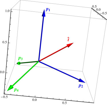
Figure 19: Maximally symmetric four-particle configuration. The blue and green pairs of particles are in back-to-back hemispheres, and the thrust axis $\mathbf{\hat{t}}$ is along the red vector, which is aligned with $\mathbf{p}_{1}+\mathbf{p}_{2}$ or $-(\mathbf{p}_{3}+\mathbf{p}_{4})$.

The angularity of this configuration can easily be computed using the representation

$$\tau_{a}=\frac{1}{Q}\,\sum_{i}\,E_{i}\,(1-|\cos\theta_{i}|)^{1-a}\;|\sin\theta_{i}|^{a}\,,$$ (163)

where $E_{i}$ is the energy and $\theta_{i}$ the angle of the i’th particle with respect to the thrust axis. This yields

$$\tau_{a}^{2,\text{max}}=4\times\frac{1}{Q}\frac{Q}{4}(1-\cos\vartheta)^{1-a}\sin^{a}\vartheta=\Bigl{(}1-\frac{\sqrt{3}}{3}\Bigr{)}^{1-a}\Bigl{(}\frac{2}{3}\Bigr{)}^{a/2}\,,$$ (164)

or in terms of the three-particle maximum $\tau_{a}^{1,\text{max}}=1/3^{1-a/2}$,

$$\tau_{a}^{2,\text{max}}=\tau_{a}^{1,\text{max}}\times 2^{a/2}(3-\sqrt{3})^{1-a}\,.$$ (165)

For some extreme values of $a$, it is possible that the maximum $\tau_{a}$ configuration is not the symmetric one in Fig. 19, as occurs for the three-particle configuration for $a\lesssim-2.6$ Hornig:2009vb . We assume that this does not occur in the four-particle configuration for the values of $a$ we consider, $-1\leq a\leq 0.5$. We in fact did not notice any anomalous deviation in the endpoints of our $\mathcal{O}(\alpha_{s}^{2})$ distributions away from this formula. The maximum three- and four-particle values of $\tau_{a}$ are illustrated in Fig. 20.

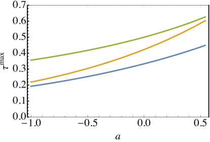
   $a$ $\tau_{a}^{1,\text{max}}$ $\tau_{a}^{2,\text{max}}$ $\tau_{a}^{\text{sph.}}$ $-1$ 0.192 0.219 0.356 $-0.75$ 0.221 0.258 0.385 $-0.5$ 0.253 0.304 0.417 $-0.25$ 0.291 0.358 0.455 0 0.333 0.423 0.5 0.25 0.382 0.498 0.553 0.5 0.439 0.587 0.616

Figure 20: The maximum values of $\tau_{a}$ for the three-particle (blue), four-particle (orange) and spherical distribution of particles (green) as a function of $a$.

References

- (1) M. Dasgupta and G. P. Salam, Event shapes in annihilation and deep inelastic scattering, J.Phys.G G30 (2004) R143, [hep-ph/0312283].
- (2) A. Gehrmann-De Ridder, T. Gehrmann, E. W. N. Glover, and G. Heinrich, NNLO corrections to event shapes in annihilation, JHEP 12 (2007) 094, [arXiv:0711.4711].
- (3) S. Weinzierl, Event shapes and jet rates in electron-positron annihilation at NNLO, JHEP 06 (2009) 041, [arXiv:0904.1077].
- (4) A. Gehrmann-De Ridder, T. Gehrmann, E. W. N. Glover, and G. Heinrich, EERAD3: Event shapes and jet rates in electron-positron annihilation at order , Comput. Phys. Commun. 185 (2014) 3331, [arXiv:1402.4140].
- (5) V. Del Duca, C. Duhr, A. Kardos, G. Somogyi, Z. Szõr, Z. Trócsányi, and Z. Tulipánt, Jet production in the CoLoRFulNNLO method: event shapes in electron-positron collisions, Phys. Rev. D94 (2016), no. 7 074019, [arXiv:1606.03453].
- (6) S. Catani, L. Trentadue, G. Turnock, and B. R. Webber, Resummation of large logarithms in event shape distributions, Nucl. Phys. B407 (1993) 3–42.
- (7) C. W. Bauer, S. Fleming, and M. E. Luke, Summing Sudakov logarithms in in effective field theory, Phys. Rev. D63 (2000) 014006, [hep-ph/0005275].
- (8) C. W. Bauer, S. Fleming, D. Pirjol, and I. W. Stewart, An effective field theory for collinear and soft gluons: Heavy to light decays, Phys. Rev. D63 (2001) 114020, [hep-ph/0011336].
- (9) C. W. Bauer, D. Pirjol, and I. W. Stewart, Soft-collinear factorization in effective field theory, Phys. Rev. D65 (2002) 054022, [hep-ph/0109045].
- (10) M. Beneke, A. Chapovsky, M. Diehl, and T. Feldmann, Soft collinear effective theory and heavy to light currents beyond leading power, Nucl.Phys. B643 (2002) 431–476, [hep-ph/0206152].
- (11) D. de Florian and M. Grazzini, The back-to-back region in energy energy correlation, Nucl. Phys. B704 (2005) 387–403, [hep-ph/0407241].
- (12) T. Becher and G. Bell, NNLL Resummation for Jet Broadening, JHEP 1211 (2012) 126, [arXiv:1210.0580].
- (13) A. Banfi, H. McAslan, P. F. Monni, and G. Zanderighi, A general method for the resummation of event-shape distributions in annihilation, JHEP 05 (2015) 102, [arXiv:1412.2126].
- (14) T. Becher and M. D. Schwartz, A precise determination of from LEP thrust data using effective field theory, JHEP 07 (2008) 034, [arXiv:0803.0342].
- (15) Y.-T. Chien and M. D. Schwartz, Resummation of heavy jet mass and comparison to LEP data, JHEP 1008 (2010) 058, [arXiv:1005.1644].
- (16) A. H. Hoang, D. W. Kolodrubetz, V. Mateu, and I. W. Stewart, -parameter distribution at including power corrections, Phys. Rev. D91 (2015), no. 9 094017, [arXiv:1411.6633].
- (17) R. A. Davison and B. R. Webber, Non-perturbative contribution to the thrust distribution in annihilation, Eur. Phys. J. C59 (2009) 13–25, [arXiv:0809.3326].
- (18) R. Abbate, M. Fickinger, A. H. Hoang, V. Mateu, and I. W. Stewart, Thrust at N3LL with Power Corrections and a Precision Global Fit for , Phys. Rev. D83 (2011) 074021, [arXiv:1006.3080].
- (19) R. Abbate, M. Fickinger, A. H. Hoang, V. Mateu, and I. W. Stewart, Precision Thrust Cumulant Moments at LL, Phys. Rev. D86 (2012) 094002, [arXiv:1204.5746].
- (20) T. Gehrmann, G. Luisoni, and P. F. Monni, Power corrections in the dispersive model for a determination of the strong coupling constant from the thrust distribution, Eur. Phys. J. C73 (2013), no. 1 2265, [arXiv:1210.6945].
- (21) A. H. Hoang, D. W. Kolodrubetz, V. Mateu, and I. W. Stewart, Precise determination of from the -parameter distribution, Phys. Rev. D91 (2015), no. 9 094018, [arXiv:1501.04111].
- (22) C. Lee and G. F. Sterman, Universality of nonperturbative effects in event shapes, eConf C0601121 (2006) A001, [hep-ph/0603066].
- (23) C. Lee and G. Sterman, Momentum flow correlations from event shapes: Factorized soft gluons and Soft-Collinear Effective Theory, Phys. Rev. D75 (2007) 014022, [hep-ph/0611061].
- (24) T. Becher and G. Bell, Enhanced nonperturbative effects through the collinear anomaly, Phys. Rev. Lett. 112 (2014), no. 18 182002, [arXiv:1312.5327].
- (25) G. Salam and D. Wicke, Hadron masses and power corrections to event shapes, JHEP 0105 (2001) 061, [hep-ph/0102343].
- (26) V. Mateu, I. W. Stewart, and J. Thaler, Power Corrections to Event Shapes with Mass-Dependent Operators, Phys.Rev. D87 (2013) 014025, [arXiv:1209.3781].
- (27) Particle Data Group Collaboration, M. Tanabashi et al., Review of particle physics, Phys. Rev. D 98 (Aug, 2018) 030001.
- (28) S. Bethke et al., Workshop on Precision Measurements of alphas, arXiv:1110.0016.
- (29) C. F. Berger, T. Kucs, and G. Sterman, Event shape / energy flow correlations, Phys. Rev. D68 (2003) 014012, [hep-ph/0303051].
- (30) Y. L. Dokshitzer, A. Lucenti, G. Marchesini, and G. P. Salam, On the QCD analysis of jet broadening, JHEP 01 (1998) 011, [hep-ph/9801324].
- (31) A. J. Larkoski, D. Neill, and J. Thaler, Jet Shapes with the Broadening Axis, JHEP 1404 (2014) 017, [arXiv:1401.2158].
- (32) M. Procura, W. J. Waalewijn, and L. Zeune, Joint resummation of two angularities at next-to-next-to-leading logarithmic order, JHEP 10 (2018) 098, [arXiv:1806.10622].
- (33) C. W. Bauer, S. Fleming, C. Lee, and G. Sterman, Factorization of event shape distributions with hadronic final states in Soft Collinear Effective Theory, Phys. Rev. D78 (2008) 034027, [arXiv:0801.4569].
- (34) A. Hornig, C. Lee, and G. Ovanesyan, Effective predictions of event shapes: Factorized, resummed, and gapped angularity distributions, JHEP 05 (2009) 122, [arXiv:0901.3780].
- (35) L. G. Almeida, S. D. Ellis, C. Lee, G. Sterman, I. Sung, and J. R. Walsh, Comparing and counting logs in direct and effective methods of QCD resummation, JHEP 1404 (2014) 174, [arXiv:1401.4460].
- (36) T. Becher, G. Bell, and M. Neubert, Factorization and Resummation for Jet Broadening, Phys.Lett. B704 (2011) 276–283, [arXiv:1104.4108].
- (37) J.-Y. Chiu, A. Jain, D. Neill, and I. Z. Rothstein, A Formalism for the Systematic Treatment of Rapidity Logarithms in Quantum Field Theory, JHEP 1205 (2012) 084, [arXiv:1202.0814].
- (38) G. P. Korchemsky, Shape functions and power corrections to the event shapes, in Continuous advances in QCD. Proceedings, 3rd Workshop, QCD’98, Minneapolis, USA, April 16-19, 1998, pp. 489–498, 1998. hep-ph/9806537.
- (39) G. P. Korchemsky and G. Sterman, Power corrections to event shapes and factorization, Nucl. Phys. B555 (1999) 335–351, [hep-ph/9902341].
- (40) C. F. Berger and G. Sterman, Scaling rule for nonperturbative radiation in a class of event shapes, JHEP 09 (2003) 058, [hep-ph/0307394].
- (41) C. F. Berger and L. Magnea, Scaling of power corrections for angularities from dressed gluon exponentiation, Phys. Rev. D70 (2004) 094010, [hep-ph/0407024].
- (42) E. Gardi, Dressed gluon exponentiation, Nucl. Phys. B622 (2002) 365–392, [hep-ph/0108222].
- (43) Y. L. Dokshitzer, G. Marchesini, and B. R. Webber, Dispersive approach to power-behaved contributions in QCD hard processes, Nucl. Phys. B469 (1996) 93–142, [hep-ph/9512336].
- (44) Y. L. Dokshitzer and B. R. Webber, Calculation of power corrections to hadronic event shapes, Phys. Lett. B352 (1995) 451–455, [hep-ph/9504219].
- (45) Y. L. Dokshitzer, A. Lucenti, G. Marchesini, and G. P. Salam, On the universality of the Milan factor for 1 / Q power corrections to jet shapes, JHEP 05 (1998) 003, [hep-ph/9802381].
- (46) G. Bell, R. Rahn, and J. Talbert, Automated Calculation of Dijet Soft Functions in Soft-Collinear Effective Theory, PoS RADCOR2015 (2016) 052, [arXiv:1512.06100].
- (47) G. Bell, R. Rahn, and J. Talbert, Two-loop anomalous dimensions of generic dijet soft functions, Nucl. Phys. B936 (2018) 520–541, [arXiv:1805.12414].
- (48) G. Bell, R. Rahn, and J. Talbert, Generic dijet soft functions at two-loop order: correlated emissions, arXiv:1812.08690.
- (49) A. Banfi, B. K. El-Menoufi, and P. F. Monni, The Sudakov radiator for jet observables and the soft physical coupling, arXiv:1807.11487.
- (50) G. Bell, A. Hornig, C. Lee, and J. Talbert, Angularities from LEP to FCC-ee, in Proceedings, Parton Radiation and Fragmentation from LHC to FCC-ee: CERN, Geneva, Switzerland, November 22-23, 2016, pp. 90–96, 2017.
- (51) A. H. Hoang and I. W. Stewart, Designing gapped soft functions for jet production, Phys. Lett. B660 (2008) 483–493, [arXiv:0709.3519].
- (52) P. Achard, O. Adriani, M. Aguilar-Benitez, J. Alcaraz, G. Alemanni, et al., Generalized event shape and energy flow studies in annihilation at 91.2–208.0 GeV, JHEP 1110 (2011) 143.
- (53) C. F. Berger, Soft gluon exponentiation and resummation. PhD thesis, SUNY, Stony Brook, 2003. hep-ph/0305076.
- (54) S. Fleming, A. H. Hoang, S. Mantry, and I. W. Stewart, Top jets in the peak region: Factorization analysis with NLL resummation, Phys. Rev. D77 (2008) 114003, [arXiv:0711.2079].
- (55) T. Becher, M. Neubert, and B. D. Pecjak, Factorization and momentum-space resummation in deep-inelastic scattering, JHEP 01 (2007) 076, [hep-ph/0607228].
- (56) T. Becher and M. Neubert, Threshold resummation in momentum space from effective field theory, Phys. Rev. Lett. 97 (2006) 082001, [hep-ph/0605050].
- (57) Z. Ligeti, I. W. Stewart, and F. J. Tackmann, Treating the quark distribution function with reliable uncertainties, Phys. Rev. D78 (2008) 114014, [arXiv:0807.1926].
- (58) A. V. Manohar, Deep inelastic scattering as using Soft-Collinear Effective Theory, Phys. Rev. D68 (2003) 114019, [hep-ph/0309176].
- (59) C. W. Bauer, C. Lee, A. V. Manohar, and M. B. Wise, Enhanced nonperturbative effects in Z decays to hadrons, Phys. Rev. D70 (2004) 034014, [hep-ph/0309278].
- (60) A. Idilbi, X.-d. Ji, and F. Yuan, Resummation of threshold logarithms in effective field theory for DIS, Drell-Yan and Higgs production, Nucl.Phys. B753 (2006) 42–68, [hep-ph/0605068].
- (61) R. N. Lee, A. V. Smirnov, and V. A. Smirnov, Analytic Results for Massless Three-Loop Form Factors, JHEP 04 (2010) 020, [arXiv:1001.2887].
- (62) T. Gehrmann, T. Huber, and D. Maitre, Two-loop quark and gluon form-factors in dimensional regularisation, Phys. Lett. B622 (2005) 295–302, [hep-ph/0507061].
- (63) T. Matsuura and W. L. van Neerven, Second Order Logarithmic Corrections to the Drell-Yan Cross-section, Z. Phys. C38 (1988) 623.
- (64) T. Matsuura, S. C. van der Marck, and W. L. van Neerven, The Calculation of the Second Order Soft and Virtual Contributions to the Drell-Yan Cross-Section, Nucl. Phys. B319 (1989) 570.
- (65) S. Moch, J. Vermaseren, and A. Vogt, The Quark form-factor at higher orders, JHEP 0508 (2005) 049, [hep-ph/0507039].
- (66) R. Kelley, M. D. Schwartz, R. M. Schabinger, and H. X. Zhu, The two-loop hemisphere soft function, Phys.Rev. D84 (2011) 045022, [arXiv:1105.3676].
- (67) P. F. Monni, T. Gehrmann, and G. Luisoni, Two-Loop Soft Corrections and Resummation of the Thrust Distribution in the Dijet Region, JHEP 1108 (2011) 010, [arXiv:1105.4560].
- (68) C. W. Bauer and A. V. Manohar, Shape function effects in and decays, Phys. Rev. D70 (2004) 034024, [hep-ph/0312109].
- (69) T. Becher and M. D. Schwartz, Direct photon production with effective field theory, JHEP 02 (2010) 040, [arXiv:0911.0681].
- (70) T. Becher and M. Neubert, Toward a NNLO calculation of the anti-BX(s) gamma decay rate with a cut on photon energy. II. Two-loop result for the jet function, Phys.Lett. B637 (2006) 251–259, [hep-ph/0603140].
- (71) T. Becher and G. Bell, The gluon jet function at two-loop order, Phys. Lett. B695 (2011) 252–258, [arXiv:1008.1936].
- (72) R. Brüser, Z. L. Liu, and M. Stahlhofen, The Three-loop Quark Jet Function, Phys. Rev. Lett. 121 (2018) 072003, [arXiv:1804.09722].
- (73) P. Banerjee, P. K. Dhani, and V. Ravindran, Gluon jet function at three loops in QCD, Phys. Rev. D98 (2018), no. 9 094016, [arXiv:1805.02637].
- (74) S. Catani and M. H. Seymour, The dipole formalism for the calculation of QCD jet cross sections at next-to-leading order, Phys. Lett. B378 (1996) 287–301, [hep-ph/9602277].
- (75) S. Catani and M. H. Seymour, A general algorithm for calculating jet cross sections in NLO QCD, Nucl. Phys. B485 (1997) 291–419, [hep-ph/9605323].
- (76) A. H. Hoang and S. Kluth, Hemisphere soft function at for dijet production in annihilation, arXiv:0806.3852.
- (77) K. G. Chetyrkin, A. L. Kataev, and F. V. Tkachov, Higher Order Corrections to Hadrons) in Quantum Chromodynamics, Phys. Lett. B85 (1979) 277.
- (78) M. Dine and J. R. Sapirstein, Higher Order QCD Corrections in Annihilation, Phys. Rev. Lett. 43 (1979) 668.
- (79) W. Celmaster and R. J. Gonsalves, An Analytic Calculation of Higher Order Quantum Chromodynamic Corrections in Annihilation, Phys. Rev. Lett. 44 (1980) 560.
- (80) Y.-T. Chien, A. Hornig, and C. Lee, Soft-collinear mode for jet cross sections in soft collinear effective theory, Phys. Rev. D93 (2016), no. 1 014033, [arXiv:1509.04287].
- (81) D. Kang, C. Lee, and I. W. Stewart, Using 1-Jettiness to Measure 2 Jets in DIS 3 Ways, Phys.Rev. D88 (2013) 054004, [arXiv:1303.6952].
- (82) G. P. Korchemsky and G. Sterman, Nonperturbative corrections in resummed cross-sections, Nucl. Phys. B437 (1995) 415–432, [hep-ph/9411211].
- (83) M. Beneke and V. M. Braun, Heavy quark effective theory beyond perturbation theory: Renormalons, the pole mass and the residual mass term, Nucl. Phys. B426 (1994) 301–343, [hep-ph/9402364].
- (84) A. Jain, I. Scimemi, and I. W. Stewart, Two-loop Jet-Function and Jet-Mass for Top Quarks, Phys. Rev. D77 (2008) 094008, [arXiv:0801.0743].
- (85) A. H. Hoang, A. Jain, I. Scimemi, and I. W. Stewart, Infrared renormalization group flow for heavy quark masses, Phys. Rev. Lett. 101 (2008) 151602, [arXiv:0803.4214].
- (86) V. Mateu. Private communication.
- (87) D. Kang, C. Lee, and I. W. Stewart, Analytic calculation of 1-jettiness in DIS at , JHEP 1411 (2014) 132, [arXiv:1407.6706].
- (88) A. Hornig, Y. Makris, and T. Mehen, Jet Shapes in Dijet Events at the LHC in SCET, JHEP 04 (2016) 097, [arXiv:1601.01319].
- (89) S. M. Freedman, Subleading Corrections To Thrust Using Effective Field Theory, arXiv:1303.1558.
- (90) I. Moult, I. W. Stewart, G. Vita, and H. X. Zhu, First Subleading Power Resummation for Event Shapes, JHEP 08 (2018) 013, [arXiv:1804.04665].
- (91) D. Bertolini, M. P. Solon, and J. R. Walsh, Integrated and Differential Accuracy in Resummed Cross Sections, Phys. Rev. D95 (2017), no. 5 054024, [arXiv:1701.07919].
- (92) O. Tarasov, A. Vladimirov, and A. Y. Zharkov, The Gell-Mann-Low Function of QCD in the Three Loop Approximation, Phys.Lett. B93 (1980) 429–432.
- (93) S. Larin and J. Vermaseren, The Three loop QCD Beta function and anomalous dimensions, Phys.Lett. B303 (1993) 334–336, [hep-ph/9302208].
- (94) T. van Ritbergen, J. A. M. Vermaseren, and S. A. Larin, The Four loop beta function in quantum chromodynamics, Phys. Lett. B400 (1997) 379–384, [hep-ph/9701390].
- (95) G. P. Korchemsky and A. V. Radyushkin, Renormalization of the Wilson Loops Beyond the Leading Order, Nucl. Phys. B283 (1987) 342–364.
- (96) S. Moch, J. Vermaseren, and A. Vogt, The Three loop splitting functions in QCD: The Nonsinglet case, Nucl.Phys. B688 (2004) 101–134, [hep-ph/0403192].