SI-HEP-2018-16

QFET-2018-10

DESY 18-078

Two-loop anomalous dimensions of
generic dijet soft functions

Guido Bell^a, Rudi Rahn^b and Jim Talbert^c

^a Theoretische Physik 1, Naturwissenschaftlich-Technische Fakultät,
Universität Siegen, Walter-Flex-Strasse 3, 57068 Siegen, Germany
^b Albert Einstein Center for Fundamental Physics, Institut für Theoretische Physik, Universität Bern, Sidlerstrasse 5, 3012 Bern, Switzerland
^c Theory Group, Deutsches Elektronen-Synchrotron (DESY), 22607 Hamburg, Germany

We present compact integral representations for the calculation of two-loop anomalous dimensions for a generic class of soft functions that are defined in terms of two light-like Wilson lines. Our results are relevant for the resummation of Sudakov logarithms for $e^{+}e^{-}$ event-shape variables and inclusive hadron-collider observables at next-to-next-to-leading logarithmic accuracy within Soft-Collinear Effective Theory (SCET). Our formalism applies to both SCET-1 and SCET-2 soft functions and we clarify the relation between the respective soft anomalous dimension and the collinear anomaly exponent. We confirm existing two-loop results for about a dozen dijet soft functions and obtain new predictions for the angularity event shape and the soft-drop jet-grooming algorithm.

1 Dijet soft functions

Scattering cross sections at large momentum transfer $Q$ are often sensitive to large logarithmic corrections that spoil the convergence of the perturbative expansion in the strong coupling $\alpha_{s}(Q)\ll 1$. By computing corrections of the form $\alpha_{s}(Q)L\sim 1$ to all orders, where $L\gg 1$ represents the large logarithm, the theoretical predictions can be systematically improved with respect to a fixed-order expansion. This reorganisation of the perturbative series – commonly called resummation – can be achieved on the basis of factorisation theorems which disentangle the relevant scales of the scattering process to all orders in perturbation theory.

The factorisation of cross sections in QCD has a long history. Traditionally, factorisation was established via an analysis of Feynman diagrams that incorporates the constraints from gauge invariance using Ward identities (see [1, 2] for a review). Alternatively, the problem can be accessed with methods from effective field theory, which separate the effects from the relevant degrees of freedom directly on the level of the Lagrangian. The two approaches have many similarities and yield identical physical results (see e.g. [3] for a detailed comparison). While we use the language of Soft-Collinear Effective Theory (SCET) [4, 5, 6] in the present work, we stress that our analysis is also relevant for resummations that are formulated in QCD.

The scattering processes of interest in this work involve two hard, massless and colour-charged partons at the Born level. Whenever the QCD radiation is confined to be low-energetic (soft) or collinear to the directions of the hard partons, the partonic cross section factorises in the schematic form

$$d\hat{\sigma}=H\cdot J_{n}\otimes J_{\bar{n}}\otimes S\,,$$ (1)

where the symbol $\otimes$ denotes a convolution in suitable kinematic variables. The hard function $H$ contains the virtual corrections to the Born process at the scale $Q^{2}$, the jet functions $J_{n}$ and $J_{\bar{n}}$ encode the effects from the collinear emissions in the directions $n^{\mu}$ and $\bar{n}^{\mu}$ of the hard partons, and the soft function $S$ describes the low-energetic cross talk between the two jets. The characteristic scales associated with the jet and soft functions are typically much smaller than $Q^{2}$, but their respective hierarchy depends on the specific observable. In fact, different hierarchies between the jet and soft scales are described by different versions of the effective theory as we will see below.

The individual factors in (1) depend on an unphysical factorisation scale, and by solving the associated renormalisation group equations (RGEs) one can resum the logarithmic corrections to the cross section to all orders. Whereas the fixed-order expansion is organised into leading order (LO) corrections, next-to-leading order (NLO) corrections, and so on, the resummed expressions refer to leading logarithmic (LL) accuracy, next-to-leading logarithmic (NLL) accuracy, etc. As in any effective field theory, the desired accuracy can then be achieved by computing anomalous dimensions and matching corrections to a given order in perturbation theory. For Sudakov problems with a double logarithm per loop order, the appropriate counting scheme is given e.g. in Table 5 of [3].

The purpose of this work is to develop a systematic framework for the computation of two-loop soft anomalous dimensions for a wide class of collider observables. The two-loop soft anomalous dimension is required for NNLL resummation and it often represents the only missing piece at this accuracy, since the two-loop hard anomalous dimension is known for arbitrary processes [7] and the two-loop jet anomalous dimension can then be extracted from the factorisation theorem (1) using RG invariance of the cross section. While one in addition needs the one-loop hard, jet, and soft matching corrections at NNLL, their computation often represents a comparably simple task.

The soft functions that enter the factorisation theorem (1) are given by vacuum matrix elements of a configuration of Wilson lines that reflect the structure of the scattering process at the Born level. More specifically, they can be written in the form

$$S(\tau,\mu)=\frac{1}{N_{c}}\;\sum_{X}\;\mathcal{M}(\tau;\{k_{i}\})\;\mathrm{Tr}\;|\langle X|\,T[S^{\dagger}_{n}(0)S_{\bar{n}}(0)]\,|0\rangle|^{2}\,,$$ (2)

where $S_{n}$ and $S_{\bar{n}}$ are soft Wilson lines extending along two light-like directions $n^{\mu}$ and $\bar{n}^{\mu}$ with $n\cdot{\bar{n}}=2$. For concreteness, we assume that the Wilson lines are in the fundamental colour representation and the definition in (2) involves a trace over colour indices as well as a generic measurement function $\mathcal{M}(\tau,\{k_{i}\})$ that provides a constraint on the soft radiation with parton momenta $\{k_{i}\}$ according to the observable under consideration. The explicit form we assume for the measurement function will be specified in the following section. Notice that up to two-loop order, it is irrelevant whether $n^{\mu}$ and $\bar{n}^{\mu}$ refer to incoming or outgoing directions [8, 9], and our results therefore equally apply to $e^{+}e^{-}$ dijet observables, one-jet observables in deep-inelastic scattering or zero-jet observables at hadron colliders. For convenience, we refer to all of these cases as dijet soft functions in the following.

The soft functions can further be classified according to the hierarchy between the jet and soft scales in the underlying factorisation theorem (1). For SCET-1 observables, the virtuality of the collinear modes is much larger than the one of the soft modes and the logarithmic corrections can be resummed using standard RG techniques. For SCET-2 observables, on the other hand, the jet and soft scales are of the same order and additional techniques like the collinear anomaly [10] or the rapidity RG [11] are needed to resum the logarithmic corrections. On the technical level, the difference between SCET-1 and SCET-2 soft functions manifests itself in the form of rapidity divergences in the phase-space integrals that are not regularised in dimensional regularisation. One therefore needs to introduce an additional regulator for SCET-2 soft functions, for which we use a symmetrised version of the analytic regulator proposed in [12].

The outline of this paper is as follows: In the next section we define more precisely which class of dijet soft functions we consider by specifying the functional form we assume for the measurement function. In Section 3 we present our results for the calculation of two-loop soft anomalous dimensions for SCET-1 type observables, and Section 4 contains the corresponding expressions for SCET-2 soft functions, for which the relevant anomalous dimension is often called the collinear anomaly exponent. The expressions we find in the SCET-1 and SCET-2 sections turn out to be similar, and we elaborate on the relation between the soft anomalous dimension and the collinear anomaly exponent in Section 5. In Section 6 we discuss several extensions of our formalism which are relevant, e.g., for jet-veto observables, multi-differential soft functions, and processes with more than two jet directions. We finally conclude in Section 7 and present further details of our calculation in two appendices.

2 Measurement function

The soft functions we consider are typically defined in Laplace (or Fourier) space. The main reason why we work in Laplace space is that the factorisation theorem (1) and the associated RGEs often take a particularly simple form in this space. For some soft functions like those associated with jet-veto observables, the RGEs are more naturally formulated in momentum (or cumulant) space, but even in this case it is possible to work with the Laplace transform to bring the soft function into the form considered in this section, and to correct for the factors associated with the inversion of the Laplace transformation at a later stage. We will come back to the discussion of jet-veto observables in Section 6.

Another advantage of the Laplace space technique is that the functions are not distribution-valued. At tree level the measurement function is then trivial and can be normalised to one, $\mathcal{M}_{0}(\tau)=1$. For a single emission with momentum $k^{\mu}$, we introduce light-cone coordinates with $k_{+}=n\cdot k$, $k_{-}=\bar{n}\cdot k$ and a vector $k_{\perp}^{\mu}$ that is transverse to $n^{\mu}$ and $\bar{n}^{\mu}$. We further parametrise the phase-space integrals in terms of the magnitude of the transverse momentum $k_{T}$, a measure of the rapidity $y_{k}$, and an angular variable $t_{k}$ as

$$k_{-}=\frac{k_{T}}{\sqrt{y_{k}}}\,,\qquad\qquad k_{+}=\sqrt{y_{k}}\,k_{T}\,,\qquad\qquad\cos\theta_{k}=1-2t_{k}\,.$$ (3)

A non-trivial dependence on the angle $\theta_{k}$ may arise when the measurement is performed with respect to a vector $v^{\mu}$ that differs from the jet axes $n^{\mu}$ and $\bar{n}^{\mu}$. If so, we project this vector onto the transverse plane and denote the angle between $\vec{v}_{\perp}$ and $\vec{k}_{\perp}$ by $\theta_{k}$.

In terms of these variables, we assume that the single-emission measurement function can be written in the form

$$\mathcal{M}_{1}(\tau;k)=\exp\big{(}-\tau\,k_{T}\,y_{k}^{n/2}\,f(y_{k},t_{k})\,\big{)}\,,$$ (4)

where the exponential reflects the fact the we work in Laplace space. We further assume that the Laplace variable $\tau$ has the dimension $1/$mass, which fixes the linear dependence on the variable $k_{T}$ on dimensional grounds. At NLO the soft functions we consider are thus characterised by a parameter $n$ and a function $f(y_{k},t_{k})$ that encodes the angular and rapidity dependence. One can show that the parameter $n$ is related to the power counting of the soft modes in the underlying factorisation theorem and that the value $n=0$ corresponds to a SCET-2 observable [13].

For our purposes, it is sufficient to adopt a pragmatic approach to determine the parameter $n$ for a given observable. After integration over $k_{T}$ and expanding in the various regulators, the expression contains logarithms of the function $f(y_{k},t_{k})$ that are multiplied by a matrix element that is divergent in the collinear limit $y_{k}\to 0$. It is therefore crucial to factor out the leading scaling in $y_{k}$, i.e. we define the parameter $n$ by the requirement that the function $f(y_{k},t_{k})$ is finite and non-zero in the limit $y_{k}\to 0$.

The considered class of soft functions may look specific, but it captures a large variety of dijet soft functions as will become clear when we discuss explicit examples below. Sample expressions for the parameter $n$ and the associated function $f(y_{k},t_{k})$ for various $e^{+}e^{-}$ and hadron-collider soft functions can be found in Table 1 of [14].

At NNLO one in addition needs to specify the double-emission measurement function. As the singularity structure of the underlying matrix element differs among the colour structures, we apply distinct phase-space parametrisations for the correlated ($C_{F}T_{F}n_{f}$, $C_{F}C_{A}$) and uncorrelated ($C_{F}^{2}$) emission contributions. These parametrisations have been chosen according to two criteria: First, they should allow us to factorise the divergences of the matrix elements and, second, they should provide a simple parametrisation of the measurement function with a two-emission equivalent of the function $f(y_{k},t_{k})$ that is finite in the singular limits of the matrix element. We found it furthermore convenient to exploit the symmetries from $n\leftrightarrow\bar{n}$ and $k\leftrightarrow l$ exchange, where $k$ and $l$ are the momenta of the emitted partons, to map the integration region onto the unit hypercube [13].

For the correlated double-emission contribution, we parametrise

$$k_{-}=\frac{ab}{1+ab}\;\frac{p_{T}}{\sqrt{y}}\,,\qquad k_{+}=\frac{b}{a+b}\;\sqrt{y}\,p_{T}\,,\qquad l_{-}=\frac{1}{1+ab}\;\frac{p_{T}}{\sqrt{y}}\,,\qquad l_{+}=\frac{a}{a+b}\;\sqrt{y}\,p_{T}\,,$$ (5)

where $p_{T}$ and $y$ are functions of the sum of the light-cone momenta, $a$ is a measure of the rapidity difference of the emitted partons, and $b$ is the ratio of their transverse momenta [14]. In general the measurement function now depends on three angles $\theta_{k}=\sphericalangle(\vec{v}_{\perp},\vec{k}_{\perp})$, $\theta_{l}=\sphericalangle(\vec{v}_{\perp},\vec{l}_{\perp})$ and $\theta_{kl}=\sphericalangle(\vec{k}_{\perp},\vec{l}_{\perp})$, and we denote the corresponding variables that are defined on the unit hypercube by $t_{k}$, $t_{l}$ and $t_{kl}$ in analogy to (3). The corresponding relation to (4) for the correlated double-emission contribution then becomes

$$\mathcal{M}_{2}^{corr}(\tau;k,l)=\exp\big{(}-\tau\,p_{T}\,y^{n/2}\,F(a,b,y,t_{k},t_{l},t_{kl})\,\big{)}\,,$$ (6)

where the dependence on $p_{T}$ is again fixed on dimensional grounds and the function $F$ is assumed to be finite and non-zero in the limit $y\to 0$. Notice that this is achieved by factorising the same power of the rapidity variable $y$ as in the one-emission case [13].

For uncorrelated emissions we use a phase-space parametrisation that itself depends on the parameter $n$,

$$k_{-} =\left(\frac{\sqrt{y_{l}}}{1+y_{l}}\right)^{n}\frac{b}{1+b}\;\frac{q_{T}}{\sqrt{y_{k}}}\,,\hskip 59.75095ptl_{-}=\left(\frac{\sqrt{y_{k}}}{1+y_{k}}\right)^{n}\frac{1}{1+b}\;\frac{q_{T}}{\sqrt{y_{l}}}\,,$$

$$k_{+} =\left(\frac{\sqrt{y_{l}}}{1+y_{l}}\right)^{n}\frac{b}{1+b}\;\sqrt{y_{k}}\,q_{T}\,,\qquad\qquad l_{+}=\left(\frac{\sqrt{y_{k}}}{1+y_{k}}\right)^{n}\frac{1}{1+b}\;\sqrt{y_{l}}\,q_{T}\,,$$ (7)

where $q_{T}$ is now the only dimensionful variable, $y_{k}$ and $y_{l}$ are measures of the rapidities of the individual partons, and $b$ reduces to the ratio of their transverse momenta for $n=0$ (the parentheses introduce rapidity-dependent weight factors for $n\neq 0$) [15]. The measurement function for uncorrelated emissions is then parametrised as

$$\mathcal{M}_{2}^{unc}(\tau;k,l)=\exp\big{(}-\tau\,q_{T}\,y_{k}^{n/2}\,y_{l}^{n/2}\,G(y_{k},y_{l},b,t_{k},t_{l},t_{kl})\,\big{)}\,,$$ (8)

where the dependence on $q_{T}$ is once more fixed on dimensional grounds and the function $G$ is supposed to be finite and non-zero in the collinear limits $y_{k}\to 0$ and $y_{l}\to 0$. The latter again requires us to factorise the rapidity variables $y_{k}$ and $y_{l}$ to the same power as in (4).

Up to NNLO the considered class of soft functions is thus characterised by the three functions $f(y_{k},t_{k})$, $F(a,b,y,t_{k},t_{l},t_{kl})$, $G(y_{k},y_{l},b,t_{k},t_{l},t_{kl})$ and a parameter $n$. As an example, we consider the soft function for $W$-production at large transverse momentum discussed in [16]. In Laplace space the one-emission measurement function reads $\mathcal{M}_{1}(\tau;k)=\exp\big{(}-\tau\,n_{J}\cdot k\big{)}$, from which we read off that the jet direction $n_{J}^{\mu}$ serves as the measurement vector $v^{\mu}$ in this case. After decomposing $n_{J}^{\mu}$ in light-cone coordinates, one has $n_{J}\cdot k=k_{-}+k_{+}-2k_{T}\cos\theta_{k}$, which in the parametrisation (3) leads to $n=-1$ and $f(y_{k},t_{k})=1+y_{k}-2\sqrt{y_{k}}(1-2t_{k})$. For two emissions, the measurement function involves the sum $n_{J}\cdot k+n_{J}\cdot l$, which for correlated emissions implies

$$F(a,b,y,t_{k},t_{l},t_{kl})=1+y-2\;\sqrt{\frac{ay}{(1+ab)(a+b)}}\;\Big{(}b(1-2t_{k})+1-2t_{l}\Big{)}\,,$$ (9)

which is finite in the limit $y\to 0$. For uncorrelated emissions, one obtains

$$G(y_{k},y_{l},b,t_{k},t_{l},t_{kl})=\frac{b(1+y_{l})(1+y_{k}-2\sqrt{y_{k}}(1-2t_{k}))}{(1+b)}+\frac{(1+y_{k})(1+y_{l}-2\sqrt{y_{l}}(1-2t_{l}))}{(1+b)}\,,$$ (10)

which is again finite in the limits $y_{k}\to 0$ and $y_{l}\to 0$.

In general the functions $F$ and $G$ are constrained by infrared and collinear safety. In the soft limit $k^{\mu}\to 0$, which corresponds to the limit $b\to 0$ in our parametrisations, one has

$$F(a,0,y,t_{k},t_{l},t_{kl})=f(y,t_{l})\,,\qquad\qquad G(y_{k},y_{l},0,t_{k},t_{l},t_{kl})=\frac{f(y_{l},t_{l})}{(1+y_{k})^{n}}\,.$$ (11)

After using the $k\leftrightarrow l$ symmetry, the soft limit $l^{\mu}\to 0$ is mapped onto the same constraints. Whenever the two emitted partons become collinear to each other, one obtains

$$F(1,b,y,t_{l},t_{l},0)=f(y,t_{l})\,,\qquad\qquad G(y_{l},y_{l},b,t_{l},t_{l},0)=\frac{f(y_{l},t_{l})}{(1+y_{l})^{n}}\,.$$ (12)

We use these relations in the following to verify if the poles of the bare soft function cancel as predicted by the RGE. The constraints also serve as a check for the derivation of the functions $F$ and $G$, and one easily verifies that they are satisfied for the example from above.

With the phase-space parametrisations and the measurement function at hand, the soft function can be evaluated in dimensional regularisation with $d=4-2\varepsilon$ dimensions. The basic strategy for the evaluation of the integrals has been outlined in [14, 15] and further details will be given in a future publication [13]. For SCET-2 soft functions with $n=0$, we implement a variant of the phase-space regulator proposed in [12],

$$\int\!d^{d}p\;\left(\frac{\nu}{p_{+}+p_{-}}\right)^{\alpha}\;\delta(p^{2})\theta(p^{0})\,,$$ (13)

which respects the $n\leftrightarrow\bar{n}$ symmetry. The rapidity divergences then manifest themselves as poles in the regulator $\alpha$.

3 Soft anomalous dimension

For observables with $n\neq 0$, the phase-space integrals are well defined in dimensional regularisation and the soft function is defined in SCET-1. Our goal then consists in determining the soft anomalous dimension $\gamma^{S}(\alpha_{s})$ from the $1/\varepsilon$ poles of the bare soft function. In the following we assume that the soft function renormalises multiplicatively in Laplace space, and that the RGE can be written in the form

$$\frac{\mathrm{d}}{\mathrm{d}\ln\mu}\;S(\tau,\mu) =-\frac{1}{n}\,\bigg{[}4\,\Gamma_{\mathrm{cusp}}(\alpha_{s})\,\ln(\mu\bar{\tau})-2\gamma^{S}(\alpha_{s})\bigg{]}\;S(\tau,\mu)\,,$$ (14)

where $\bar{\tau}=\tau e^{\gamma_{E}}$ and $\Gamma_{\mathrm{cusp}}(\alpha_{s})$ is the universal cusp anomalous dimension. Notice that we define the soft anomalous dimension with a prefactor $2/n$, where $n$ reflects the scaling of the observable in the soft-collinear limit as discussed in the previous section. The leading coefficients in the expansion of the cusp anomalous dimension $\Gamma_{\mathrm{cusp}}(\alpha_{s})=\sum_{n=0}^{\infty}\,\Gamma_{n}(\frac{\alpha_{s}}{4\pi})^{n+1}$ are $\Gamma_{0}=4C_{F}$ and $\Gamma_{1}/\Gamma_{0}=(67/9-\pi^{2}/3)C_{A}-20/9\,T_{F}n_{f}.$

Expanding the soft anomalous dimension as $\gamma^{S}(\alpha_{s})=\sum_{n=0}^{\infty}\,\gamma^{S}_{n}\,(\frac{\alpha_{s}}{4\pi})^{n+1}$, we can determine its leading coefficient from the NLO calculation that has been described in detail in [14]. For the class of soft functions defined in (4), we find

$$\gamma^{S}_{0} =-\frac{16C_{F}}{\pi}\int_{0}^{1}\!dt_{k}\;\,\frac{\ln f(0,t_{k})}{\sqrt{\rule{0.0pt}{9.95845pt}4t_{k}\bar{t}_{k}}}$$ (15)

with $\bar{t}_{k}=1-t_{k}$. Notice that the single-emission function $f(y_{k},t_{k})$ enters this formula only in the collinear limit $y_{k}\to 0$, which explains why the one-loop anomalous dimension is identical for many observables. With the normalisation adopted in (14), $\gamma^{S}_{0}$ is moreover independent of the parameter $n$.

At NNLO the soft anomalous dimension receives contributions from three colour structures,

$$\gamma_{1}^{S} =\gamma_{1}^{n_{f}}\,C_{F}T_{F}n_{f}\,+\,\gamma_{1}^{C_{A}}\,C_{F}C_{A}\,+\,\gamma_{1}^{C_{F}}\,C_{F}^{2}\,.$$ (16)

The first two terms refer to the correlated emission contribution, which according to (6) can be expressed in terms of the function $F(a,b,y,t_{k},t_{l},t_{kl})$. Similar to the one-loop result, it turns out that this function is only required in the limit $y\to 0$, and we obtain

$$\gamma^{n_{f}}_{1} =\frac{224}{27}-\frac{4\pi^{2}}{9}+\frac{64}{9\pi}\,\int_{0}^{1}\!dt_{l}\;\,\frac{5+3\ln(16t_{l}\bar{t}_{l})}{\sqrt{\rule{0.0pt}{9.95845pt}4t_{l}\bar{t}_{l}}}\;\ln f(0,t_{l})$$

$$\quad+\frac{1}{\pi^{2}}\int_{0}^{1}\!da\int_{0}^{1}\!db\int_{0}^{1}\!dt_{l}\int_{0}^{1}\!dt_{kl}\;\frac{k_{1}(a,b,t_{kl})}{\sqrt{\rule{0.0pt}{9.95845pt}16t_{l}\bar{t}_{l}t_{kl}\bar{t}_{kl}}}\;\,\mathcal{F}(a,b,t_{l},t_{kl})\,,$$

$$\gamma^{C_{A}}_{1} =-\frac{808}{27}+\frac{11\pi^{2}}{9}+28\zeta_{3}-\frac{16}{9\pi}\,\int_{0}^{1}\!dt_{l}\;\,\frac{67-3\pi^{2}+33\ln(16t_{l}\bar{t}_{l})}{\sqrt{\rule{0.0pt}{9.95845pt}4t_{l}\bar{t}_{l}}}\;\ln f(0,t_{l})$$

$$\quad+\frac{1}{\pi^{2}}\int_{0}^{1}\!da\int_{0}^{1}\!db\int_{0}^{1}\!dt_{l}\int_{0}^{1}\!dt_{kl}\;\frac{k_{2}(a,b,t_{kl})}{\sqrt{\rule{0.0pt}{9.95845pt}16t_{l}\bar{t}_{l}t_{kl}\bar{t}_{kl}}}\;\mathcal{F}(a,b,t_{l},t_{kl})\,,$$ (17)

where $\bar{t}_{l}$ and $\bar{t}_{kl}$ are defined in analogy to $\bar{t}_{k}$, and

$$\mathcal{F}(a,b,t_{l},t_{kl}) =\ln\frac{F_{A}(a,b,0,t_{k}^{+},t_{l},t_{kl})}{f(0,t_{l})}+\ln\frac{F_{B}(a,b,0,t_{k}^{+},t_{l},t_{kl})}{f(0,t_{l})}+(t_{k}^{+}\to t_{k}^{-})$$ (18)

encodes the dependence on the two-emission measurement function. Here the subscripts $A$ and $B$ refer to two different versions of the measurement function with

$$F_{A}(a,b,y,t_{k},t_{l},t_{kl}) =F(a,b,y,t_{k},t_{l},t_{kl})\,,$$

$$F_{B}(a,b,y,t_{k},t_{l},t_{kl}) =F(1/a,b,y,t_{k},t_{l},t_{kl})\,,$$ (19)

which arise because of certain remappings that are needed to constrain the integration region onto the unit hypercube [13]. We further introduced the angular variables

$$t_{k}^{\pm}=t_{l}+t_{kl}-2t_{l}t_{kl}\pm 2\sqrt{t_{l}\bar{t}_{l}t_{kl}\bar{t}_{kl}}$$ (20)

as well as the integration kernels

$$k_{1}(a,b,t_{kl}) =\frac{128a}{(a+b)^{2}(1+ab)^{2}}\;\bigg{\{}\frac{b(1-a^{2})^{2}}{[(1-a)^{2}+4at_{kl}]^{2}}-\frac{(a+b)(1+ab)}{(1-a)^{2}+4at_{kl}}\bigg{\}}\,,$$

$$k_{2}(a,b,t_{kl}) =-\frac{32}{ab(a+b)^{2}(1+ab)^{2}}\;\bigg{\{}\frac{2a^{2}b^{2}(1-a^{2})^{2}}{[(1-a)^{2}+4at_{kl}]^{2}}-(a+b)(1+ab)$$

$$\qquad\times\bigg{[}b(1+a^{2})+2a(1+b^{2})-\frac{b(1-a^{2})^{2}+2a(1+a^{2})(1+b^{2})}{(1-a)^{2}+4at_{kl}}\bigg{]}\bigg{\}}\,.$$ (21)

The third colour structure in (16) is only non-zero for observables that violate the non-Abelian exponentiation (NAE) theorem [17, 18]. For observables that obey NAE, the two-emission measurement function factorises in Laplace space into a product of single-emission functions, and one easily verifies that $\gamma^{C_{F}}_{1}$ vanishes in this case. With our general ansatz (8) in terms of a non-factorisable function $G(y_{k},y_{l},b,t_{k},t_{l},t_{kl})$, it is however non-trivial to show that $\gamma^{C_{F}}_{1}$ is zero for observables that obey NAE. Moreover, we find that the $1/\varepsilon^{2}$ poles only cancel as predicted by the RGE (14) if the constraint (54) in Appendix A is satisfied. For further details on the calculation of the $C_{F}^{2}$ contribution we refer to the appendix, but we stress once more that the following result for $\gamma^{C_{F}}_{1}$ only holds if the condition (54) is fulfilled. Explicitly, we find

$$\gamma^{C_{F}}_{1} =\frac{128}{\pi}\,\int_{0}^{1}\!dy\int_{0}^{1}\!dt_{l}\;\,\frac{1}{\sqrt{\rule{0.0pt}{9.95845pt}4t_{l}\bar{t}_{l}}}\;\,\frac{1}{y}\;\ln^{2}\left(\frac{(1+y)^{n}\,f(y,t_{l})}{f(0,t_{l})}\right)$$

$$\quad+\frac{256}{\pi}\,\int_{0}^{1}\!dy\int_{0}^{1}\!dt_{l}\;\,\frac{\ln f(0,t_{l})}{\sqrt{\rule{0.0pt}{9.95845pt}4t_{l}\bar{t}_{l}}}\;\frac{\ln f(y,t_{l})}{y_{+}}$$

$$\quad-\frac{512}{\pi^{2}}\,\int_{0}^{1}\!dt_{k}\;\,\frac{\ln f(0,t_{k})}{\sqrt{\rule{0.0pt}{9.95845pt}4t_{k}\bar{t}_{k}}}\;\int_{0}^{1}\!dy\int_{0}^{1}\!dt_{l}\;\,\frac{1}{\sqrt{\rule{0.0pt}{9.95845pt}4t_{l}\bar{t}_{l}}}\;\frac{\ln f(y,t_{l})}{y_{+}}$$

$$\quad-\frac{128}{\pi^{2}}\int_{0}^{1}\!dy\int_{0}^{1}\!db\int_{0}^{1}\!dt_{l}\int_{0}^{1}\!dt_{kl}\;\frac{1}{\sqrt{\rule{0.0pt}{9.95845pt}16t_{l}\bar{t}_{l}t_{kl}\bar{t}_{kl}}}\;\,\frac{\mathcal{G}_{1}(y,b,t_{l},t_{kl})}{y_{+}b_{+}}\,$$

$$\quad-\frac{64}{\pi^{2}}\int_{0}^{1}\!dr\int_{0}^{1}\!db\int_{0}^{1}\!dt_{l}\int_{0}^{1}\!dt_{kl}\;\frac{1}{\sqrt{\rule{0.0pt}{9.95845pt}16t_{l}\bar{t}_{l}t_{kl}\bar{t}_{kl}}}\;\,\frac{\mathcal{G}_{2}(r,b,t_{l},t_{kl})}{r_{+}b_{+}}$$ (22)

up to an additional contribution in (55), which we conjecture to vanish for all observables. Here the notation $1/x_{+}$ refers to a plus-distribution defined as $\int_{0}^{1}\!dx\,f(x)/x_{+}=\int_{0}^{1}\!dx\,(f(x)-f(0))/x$. The dependence on the two-emission measurement function is furthermore now encoded in

$$\mathcal{G}_{1}(y,b,t_{l},t_{kl}) =\ln G_{A_{1}}(y,0,b,t_{k}^{+},t_{l},t_{kl})+\ln G_{A_{2}}(y,0,b,t_{k}^{+},t_{l},t_{kl})$$

$$\quad+\ln G_{B_{1}}(y,0,b,t_{k}^{+},t_{l},t_{kl})+\ln G_{B_{2}}(y,0,b,t_{k}^{+},t_{l},t_{kl})+(t_{k}^{+}\to t_{k}^{-})\,,$$

$$\mathcal{G}_{2}(r,b,t_{l},t_{kl}) =\ln G_{A_{1}}(0,r,b,t_{k}^{+},t_{l},t_{kl})+\ln G_{A_{2}}(0,r,b,t_{k}^{+},t_{l},t_{kl})$$

$$\quad+\ln G_{B_{1}}(0,r,b,t_{k}^{+},t_{l},t_{kl})+\ln G_{B_{2}}(0,r,b,t_{k}^{+},t_{l},t_{kl})+(t_{k}^{+}\to t_{k}^{-})\,,$$ (23)

where the subscripts $A$ and $B$ refer to the same and opposite hemisphere contributions, respectively, with

$$G_{A}(y_{k},y_{l},b,t_{k},t_{l},t_{kl}) =G(y_{k},y_{l},b,t_{k},t_{l},t_{kl})\,,$$

$$G_{B}(y_{k},y_{l},b,t_{k},t_{l},t_{kl}) =y_{l}^{-n}\;G(y_{k},1/y_{l},b,t_{k},t_{l},t_{kl})\,,$$ (24)

and we have disentangled the scalings in the joint limit $y_{k}\to 0$ and $y_{l}\to 0$ at a fixed ratio $y_{k}/y_{l}$ from those of the subsequent limits with $y_{k}/y_{l}\to 0$ or $y_{l}/y_{k}\to 0$ via

$$G_{A_{1}}(y,r,b,t_{k},t_{l},t_{kl}) =G_{A}(y,ry,b,t_{k},t_{l},t_{kl})\,,$$

$$G_{A_{2}}(y,r,b,t_{k},t_{l},t_{kl}) =G_{A}(ry,y,b,t_{k},t_{l},t_{kl})\,,$$ (25)

and similarly for region $B$.

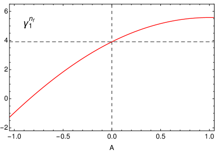
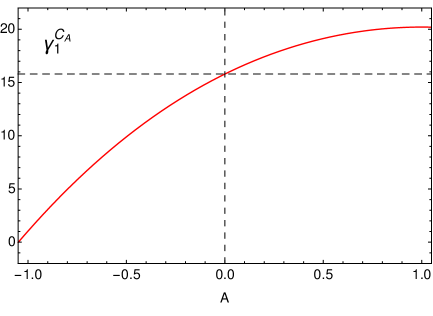
Figure 1: Two-loop soft anomalous dimension of the $e^{+}e^{-}$ event-shape variable angularities. The dashed line indicates the thrust number, which is known analytically from [21, 22].

Equations (15), (17) and (22) represent the main result of this section; they directly yield the soft anomalous dimension once the measurement functions for an observable have been determined. Let us now illustrate how to use these equations with a few examples. For simplicity, we focus here on soft functions that obey NAE such that $\gamma^{C_{F}}_{1}=0$ in the following. We will come back to the discussion of NAE-violating observables in Section 6.

We first consider the soft function relevant for threshold resummation in Drell-Yan production [19, 20], which is characterised by $n=-1$, $f(y_{k},t_{k})=1+y_{k}$ and $F(a,b,y,t_{k},t_{l},t_{kl})=1+y$. It turns out that the integrals in (15) and (17) vanish for this observable and so $\gamma^{S}_{0}=0$, $\gamma^{n_{f}}_{1}=224/27-4/9\,\pi^{2}$ and $\gamma^{C_{A}}_{1}=-808/27+11/9\,\pi^{2}+28\zeta_{3}$, which agrees with the findings from [19, 20]. With the explicit formulae for the measurement function from the previous section, one similarly shows that the soft anomalous dimension for $W$-production at large transverse momentum is identical (in our normalisation), which is in line with the calculation in [16]. The same is true for certain event-shape variables like thrust and C-parameter [21, 22, 23].

As a new application of our formalism, we consider the $e^{+}e^{-}$ event shape angularities [24]. In this case one has $n=1-A$, $f(y_{k},t_{k})=1$ (for $0\leq y_{k}\leq 1$), and

$$F_{A}(a,b,0,t_{k},t_{l},t_{kl}) =\frac{a+a^{A}b}{a+b}\;\bigg{(}\frac{a+b}{a(1+ab)}\bigg{)}^{A/2}\,,$$

$$F_{B}(a,b,0,t_{k},t_{l},t_{kl}) =\frac{a^{A}+ab}{1+ab}\;\bigg{(}\frac{1+ab}{a(a+b)}\bigg{)}^{A/2}\,,$$ (26)

where $A<1$ is the value of the angularity. At NLO this again implies $\gamma^{S}_{0}=0$ in agreement with [25] and at NNLO the integral representations in (17) can be evaluated numerically. The result is shown in Figure 1, which represents the first calculation of the two-loop soft anomalous dimension for this observable. Our result can be used to extend existing resummations for the angularity distributions to NNLL accuracy [26, 27, 28].

4 Collinear anomaly exponent

For observables with $n=0$, the phase-space integrals are sensitive to rapidity divergences and the soft function is defined in SCET-2. In this case we implement the phase-space regulator $\alpha$ as discussed at the end of Section 2, and we determine the collinear anomaly exponent $\mathcal{F}(\tau,\mu)$ from the $1/\alpha$ poles of the bare soft function. The collinear anomaly exponent controls the logarithmic corrections in the rapidity scale $\nu$ [10],

$$S(\tau,\mu,\nu) =(\nu^{2}\bar{\tau}^{2})^{-\mathcal{F}(\tau,\mu)}\;W_{S}(\tau,\mu)\,,$$ (27)

which can also be viewed as the solution of a rapidity RGE [11]. The renormalised anomaly exponent satisfies the RGE

$$\frac{\mathrm{d}}{\mathrm{d}\ln\mu}\;\mathcal{F}(\tau,\mu) =2\,\Gamma_{\mathrm{cusp}}(\alpha_{s})\,,$$ (28)

which has the two-loop solution

$$\mathcal{F}(\tau,\mu) =\left(\frac{\alpha_{s}}{4\pi}\right)\Big{\{}2\Gamma_{0}\,L+d_{1}\Big{\}}+\left(\frac{\alpha_{s}}{4\pi}\right)^{2}\Big{\{}2\beta_{0}\Gamma_{0}\,L^{2}+2\left(\Gamma_{1}+\beta_{0}d_{1}\right)L+d_{2}\Big{\}},$$ (29)

where $L=\ln(\mu\bar{\tau})$ and $\beta_{0}=11/3\,C_{A}-4/3\,T_{F}n_{f}$ is the one-loop coefficient of the beta function.

We then proceed along the lines of the previous section to determine the non-logarithmic terms of the collinear anomaly exponent $d_{1}$ and $d_{2}$. At NLO we find that the one-loop anomaly exponent has a similar integral representation as in (15) with

$$d_{1}=-\gamma^{S}_{0}\,.$$ (30)

At NNLO we again distinguish between correlated and uncorrelated emission contributions, and we decompose the two-loop anomaly exponent according to three colour structures,

$$d_{2} =d_{2}^{\,n_{f}}\,C_{F}T_{F}n_{f}\,+\,d_{2}^{\,C_{A}}\,C_{F}C_{A}\,+\,d_{2}^{\,C_{F}}\,C_{F}^{2}\,.$$ (31)

Intriguingly, we again find similar integral representations as in (17) and (22) with

$$d_{2}^{\,n_{f}} =-\gamma^{n_{f}}_{1}-\frac{4\pi^{2}}{3}-\frac{64}{3\pi}\,\int_{0}^{1}\!dt_{l}\;\,\frac{\ln f(0,t_{l})}{\sqrt{\rule{0.0pt}{9.95845pt}4t_{l}\bar{t}_{l}}}\;\ln\bigg{(}\frac{f(0,t_{l})}{16t_{l}\bar{t}_{l}}\bigg{)}\,,$$

$$d_{2}^{\,C_{A}} =-\gamma^{C_{A}}_{1}+\frac{11\pi^{2}}{3}+\frac{176}{3\pi}\,\int_{0}^{1}\!dt_{l}\;\,\frac{\ln f(0,t_{l})}{\sqrt{\rule{0.0pt}{9.95845pt}4t_{l}\bar{t}_{l}}}\;\ln\bigg{(}\frac{f(0,t_{l})}{16t_{l}\bar{t}_{l}}\bigg{)}\,,$$

$$d_{2}^{\,C_{F}} =-\gamma^{C_{F}}_{1}\,,$$ (32)

where the same remarks apply for the $C_{F}^{2}$ contribution as in the previous section, namely our result for $d_{2}^{\,C_{F}}$ only holds if the constraint (54) is satisfied and there exists an additional contribution to $d_{2}^{\,C_{F}}$ that is specified in (56) and which we conjecture to vanish for all observables.

We again illustrate the use of equations (30) and (32) with a few examples that respect NAE such that $d_{2}^{\,C_{F}}=0$. We first consider the soft function for the jet broadening event shape, neglecting any complications from recoil effects. It is specified by $f(y_{k},t_{k})=1/2$ and

$$F(a,b,y,t_{k},t_{l},t_{kl}) =\sqrt{\frac{a}{(1+ab)(a+b)}}\;\frac{1+b}{2}\,,$$ (33)

which yields $d_{1}=-8C_{F}\ln 2$. The two-loop anomaly exponent can also be obtained analytically in our setup, and we find

$$d_{2}^{\,n_{f}} =-\frac{32}{3}\ln^{2}2+\frac{320}{9}\ln 2-\frac{128}{27}-\frac{8\pi^{2}}{3}\,,$$

$$d_{2}^{\,C_{A}} =\frac{88}{3}\ln^{2}2-\left(\frac{1048}{9}+\frac{16\pi^{2}}{3}\right)\ln 2+\frac{760}{27}+\frac{22\pi^{2}}{3}+8\zeta_{3}\,,$$ (34)

which agrees with the results from [30].

Another interesting application is the soft function for transverse-momentum resummation in Drell-Yan production [31, 32]. In this case, one has $f(y_{k},t_{k})=-2i(1-2t_{k})$ and

$$F(a,b,y,t_{k},t_{l},t_{kl}) =-2i\;\sqrt{\frac{a}{(1+ab)(a+b)}}\;\Big{(}b(1-2t_{k})+1-2t_{l}\Big{)}\,,$$ (35)

where the global factor of $i$ arises from taking a Fourier instead of a Laplace transformation. Although the imaginary unit may lead to non-trivial phases for the individual terms in (32), the imaginary parts must cancel in their sum since the anomaly exponent is real. The results from Sections 3 and 4 can therefore equally be applied to soft functions that are defined in Fourier space, and for the specific case of transverse-momentum resummation, we find $d_{1}=0$ at NLO, and $d_{2}^{\,n_{f}}=-8.294(8)$ and $d_{2}^{\,C_{A}}=-3.727(11)$ at NNLO, which is in excellent agreement with the analytic results $d_{2}^{\,n_{f}}=-224/27$ and $d_{2}^{\,C_{A}}=808/27-28\zeta_{3}$ from [10, 33].

5 Relation between $\gamma^{S}$ and $\mathcal{F}$

The results of the previous section suggest that there exists a relation between the soft anomalous dimension $\gamma^{S}(\alpha_{s})$ and the collinear anomaly exponent $\mathcal{F}(\tau,\mu)$, which we explore more generally in this section. As we are mainly interested in understanding the mismatch between $\gamma_{1}$ and $d_{2}$ that arises at NNLO in (32), we focus in this section on observables that are consistent with NAE. For concreteness, we consider the angularity event shape [24]

$$e_{A}(X)=\sum_{i\in X}\,|k_{\perp}^{i}|\;e^{-|\eta_{i}|\,(1-A)}\,,$$ (36)

where the transverse momentum $k_{\perp}^{i}$ and the rapidity $\eta_{i}$ are measured with respect to the thrust axis. The angularities obey a SCET-1 type factorisation theorem for $A<1$ in the dijet limit $e_{A}\ll 1$ [25]. The case $A=1$, on the other hand, corresponds to the event shape total jet broadening, which is a SCET-2 observable [34, 11]. In the limit $A\to 1$, we can thus examine the transition from SCET-1 to SCET-2 and in this way we can connect the soft anomalous dimension with the collinear anomaly exponent. Our analysis is inspired by and extends the study of [29].

The starting point of our analysis is the resummed angularity distribution in Laplace space,

$$\frac{1}{\sigma_{0}}\frac{\mathrm{d}\sigma}{\mathrm{d}\tau_{A}} =e^{4\mathcal{S}(\mu_{h},\mu_{j})-2A_{H}(\mu_{h},\mu_{j})+\frac{4}{1-A}\mathcal{S}(\mu_{s},\mu_{j})+\frac{2}{1-A}A_{S}(\mu_{j},\mu_{s})}\;\left(\frac{Q^{2}}{\mu_{h}^{2}}\right)^{-2A_{\Gamma}(\mu_{h},\mu_{j})}\;\left(\mu_{s}\bar{\tau}_{A}\right)^{-\frac{4}{1-A}A_{\Gamma}(\mu_{j},\mu_{s})}$$

$$\quad\times H(Q,\mu_{h})\;J(\tau_{A},\mu_{j})\;J(\tau_{A},\mu_{j})\;S(\tau_{A},\mu_{s})\,,$$ (37)

where $\tau_{A}$ represents the Laplace-conjugate variable to $e_{A}$ and the scales $\mu_{i}$ with $i=h,j,s$ are to be chosen such that the quantities in the second line do not contain large logarithmic corrections. The evolution kernels

$$\mathcal{S}(\mu_{1},\mu_{2}) =-\int_{\alpha_{s}(\mu_{1})}^{\alpha_{s}(\mu_{2})}d\alpha\;\frac{\Gamma_{\mathrm{cusp}}(\alpha)}{\beta(\alpha)}\;\int_{\alpha_{s}(\mu_{1})}^{\alpha}\,\frac{d\alpha^{\prime}}{\beta(\alpha^{\prime})}\,,$$

$$A_{i}(\mu_{1},\mu_{2}) =-\int_{\alpha_{s}(\mu_{1})}^{\alpha_{s}(\mu_{2})}d\alpha\;\frac{\gamma^{i}(\alpha)}{\beta(\alpha)}$$ (38)

for $i=H,S$ and $A_{\Gamma}(\mu_{1},\mu_{2})$, which is defined as $A_{i}(\mu_{1},\mu_{2})$ but with $\gamma^{i}$ replaced by $\Gamma_{\mathrm{cusp}}$, then resum the logarithmic corrections to all orders in perturbation theory.

Whereas the above expression holds for $A<1$, one can apply the collinear anomaly technique [10] or, equivalently, the rapidity RG [11] to resum the logarithmic corrections to the (recoil-free) broadening distribution in the dijet limit. In this case, one finds

$$\frac{1}{\sigma_{0}}\frac{\mathrm{d}\sigma}{\mathrm{d}\tau_{1}} =e^{4\mathcal{S}(\mu_{h},\mu_{s})-2A_{H}(\mu_{h},\mu_{s})}\;\left(\frac{Q^{2}}{\mu_{h}^{2}}\right)^{-2A_{\Gamma}(\mu_{h},\mu_{j})}\;\left(\frac{\nu_{j}^{2}}{\nu_{s}^{2}}\right)^{-\mathcal{F}(\tau_{1},\mu_{s})}$$

$$\quad\times H(Q,\mu_{h})\;J(\tau_{1},\mu_{j},\nu_{j})\;J(\tau_{1},\mu_{j},\nu_{j})\;S(\tau_{1},\mu_{s},\nu_{s})\,,$$ (39)

where $\mathcal{F}(\tau_{1},\mu_{s})$ is the collinear anomaly exponent and $\nu_{j}$ and $\nu_{s}$ are rapidity scales. Notice that in our notation we distinguish between the SCET-2 jet and soft functions and the corresponding ones in (37) only by their arguments.

Our goal thus consists in connecting equations (37) and (39) in the limit $A\to 1$. To this end, we first compare the terms that resum the double-logarithmic corrections in the RGEs of the respective soft functions,

$$\frac{\mathrm{d}\ln S(\tau_{A},\mu_{s})}{\mathrm{d}\ln\mu_{s}} =-\frac{4}{1-A}\;\Gamma_{\mathrm{cusp}}(\alpha_{s})\ln(\mu_{s}\bar{\tau}_{A})+\ldots\,,$$

$$\frac{\mathrm{d}\ln S(\tau_{1},\mu_{s},\nu_{s})}{\mathrm{d}\ln\mu_{s}} =4\,\Gamma_{\mathrm{cusp}}(\alpha_{s})\ln(\mu_{s}\bar{\tau}_{1})-4\,\Gamma_{\mathrm{cusp}}(\alpha_{s})\ln(\nu_{s}\bar{\tau}_{1})+\ldots\,.$$ (40)

As the two equations must coincide in the limit $A\to 1$, we obtain a relation between the soft RG scale $\mu_{s}$ and the corresponding rapidity scale $\nu_{s}$,

$$\mu_{s} =\nu_{s}^{\frac{1-A}{2-A}}\;\bar{\tau}_{1}^{-\frac{1}{2-A}}\,.$$ (41)

Proceeding similarly for the jet functions, one obtains

$$\frac{\mu_{j}}{\mu_{s}} =\left(\frac{\nu_{j}}{\nu_{s}}\right)^{\frac{1-A}{2-A}}\,\xlongrightarrow{A\to 1\;}\,1+(1-A)\,\ln\frac{\nu_{j}}{\nu_{s}}+\mathcal{O}(1-A)^{2}\,$$

which reveals that the jet and soft RG scales coincide in the strict broadening limit, and that the rapidity logarithms emerge in the first-order correction.

The preceding relation can be used to analyse the RG kernels in (37) that are multiplied by a divergent prefactor in the broadening limit. This yields

$$\frac{4}{1-A}\,\,\mathcal{S}(\mu_{s},\mu_{j}) \,\xlongrightarrow{A\to 1\;}\,\mathcal{O}(1-A)\,,$$

$$\frac{2}{1-A}\;A_{S}(\mu_{j},\mu_{s}) \,\xlongrightarrow{A\to 1\;}\,\gamma^{S}\big{(}\alpha_{s}(1/\bar{\tau}_{1})\big{)}\ln\frac{\nu_{j}^{2}}{\nu_{s}^{2}}+\mathcal{O}(1-A)\,,$$ (42)

which shows that the rapidity logarithms are indeed controlled by the soft anomalous dimension. In order to connect equations (37) and (39), we still need, however, to examine the matching corrections more closely.

It turns out that the SCET-1 matching corrections are by themselves divergent in the limit $A\to 1$. Up to the considered NNLL accuracy, they can be written in the form

$$J(\tau_{A},\mu_{j}) \,\xlongrightarrow{A\to 1\;}\,1+\frac{\alpha_{s}(\mu_{j})}{4\pi}\bigg{\{}\gamma_{0}^{S}\,\ln\frac{Q}{\nu_{j}}+\frac{d^{\prime}_{1}}{2(1-A)}+c_{1}^{J}+\mathcal{O}(1-A)\bigg{\}}\,,$$

$$S(\tau_{A},\mu_{s}) \,\xlongrightarrow{A\to 1\;}\,1+\frac{\alpha_{s}(\mu_{s})}{4\pi}\bigg{\{}2\gamma_{0}^{S}\,\ln(\nu_{s}\bar{\tau}_{1})-\frac{d^{\prime}_{1}}{(1-A)}+c_{1}^{S}+\mathcal{O}(1-A)\bigg{\}}\,.$$ (43)

Whereas the regular terms in the limit $A\to 1$ match onto the corresponding expressions in the SCET-2 matching corrections (after identifying $d_{1}=-\gamma_{0}^{S}$ as shown below), the pole terms in $(1-A)$ induce a new contribution. Although the poles themselves cancel in the product of jet and soft functions, their interplay generates a non-trivial correction since the coupling constants in (43) are evaluated at different scales. In total, we find that the ratio of SCET-1 and SCET-2 matching corrections becomes

$$\frac{J(\tau_{A},\mu_{j})\;J(\tau_{A},\mu_{j})\;S(\tau_{A},\mu_{s})}{J(\tau_{1},\mu_{j},\nu_{j})\;J(\tau_{1},\mu_{j},\nu_{j})\;S(\tau_{1},\mu_{s},\nu_{s})} \,\xlongrightarrow{A\to 1\;}\,1-\left(\frac{\alpha_{s}(1/\bar{\tau}_{1})}{4\pi}\right)^{2}\beta_{0}\,d^{\prime}_{1}\,\ln\frac{\nu_{j}^{2}}{\nu_{s}^{2}}\,,$$ (44)

which must be interpreted as an additional contribution to the anomaly exponent.

We now have assembled all pieces to combine equations (37) and (39) in the limit $A\to 1$ and to connect the soft anomalous dimension with the collinear anomaly exponent. Up to NNLO, we find

$$d_{1} =-\gamma^{S}_{0}\,,$$

$$d_{2} =-\gamma^{S}_{1}+\beta_{0}\,d^{\prime}_{1}\,,$$ (45)

which explains the relation and the mismatch between $d_{2}$ and $\gamma^{S}_{1}$ that we found earlier in (32). The coefficient $d^{\prime}_{1}$, which we introduced in (43) as the coefficient of the $(1-A)$ pole in the one-loop matching corrections, can furthermore be identified with the $\mathcal{O}(\varepsilon)$ piece of the one-loop anomaly exponent,

$$\mathcal{F}(\tau_{1},\mu_{s}=1/\bar{\tau}_{1}) =\left(\frac{\alpha_{s}}{4\pi}\right)\Big{\{}d_{1}+d^{\prime}_{1}\,\varepsilon\Big{\}}+\mathcal{O}(\alpha_{s}^{2})\,.$$ (46)

Our results in (45) resemble similar relations between the soft anomalous dimension and the collinear anomaly exponent that were found earlier in [35, 36]. The physical contents of these relations and our results is, however, different. Whereas the authors in [35, 36] found a relation between the anomaly exponent for transverse-momentum resummation and the anomalous dimension for threshold resummation using either bootstrapping [35] or conformal-mapping [36] techniques, our results assume that the same measurement functions $f(y_{k},t_{k})$, $F(a,b,y,t_{k},t_{l},t_{kl})$ and $G(y_{k},y_{l},b,t_{k},t_{l},t_{kl})$ enter the SCET-1 formulae (15), (17), (22) and the corresponding SCET-2 relations (30) and (32). We therefore cannot connect the quantities for transverse-momentum and threshold resummation in our formalism, but in contrast our result can be used, for instance, to determine the (recoil-free) jet broadening anomaly exponent directly from the angularity soft anomalous dimension for $A=1$.

6 Generalisation to other observables

Our findings so far are limited to dijet soft functions with a measurement function that can be written in the form (4), (6) and (8). In this section we consider three types of generalisations: (i) cumulant soft functions with measurement functions that involve theta functions instead of exponentials, (ii) multi-differential soft functions that depend on more than one Laplace variable and (iii) $N$-jet soft functions that are defined in terms of $N>2$ light-like directions. We will address each of these extensions in turn.

Cumulant soft functions: Soft functions for jet-veto and jet-grooming observables typically involve measurement functions that are formulated in terms of a theta function, which reflects the fact that the jet veto/groomer provides a cutoff for the phase-space integrations of the soft radiation. Our formalism can easily be generalised to this class of observables. To do so, we write the one-emission measurement function of a cumulant soft function $\widehat{S}(\omega,\mu)$ in the form

$$\widehat{\mathcal{M}}_{1}(\omega;k)=\theta\big{(}\omega-k_{T}\,y_{k}^{n/2}\,f(y_{k},t_{k})\,\big{)}\,,$$ (47)

and similarly for the two-emission functions. By taking the Laplace transform with respect to the cutoff variable $\omega$, one can then bring the measurement function into the form considered in Section 2. We can thus calculate the bare soft function in Laplace space using the strategy from the previous sections, and we finally have to invert the Laplace transformation which reshuffles some of the coefficients in the $\varepsilon$ and $\alpha$ expansions. Assuming that the RGEs for cumulant soft functions $\widehat{S}(\omega,\mu)$ take a similar form as (14) and (28), we can derive master formulae for the calculation of the soft anomalous dimension $\widehat{\gamma}^{S}(\alpha_{s})$ and the anomaly exponent $\widehat{\mathcal{F}}(\omega,\mu)$ for this class of observables. Specifically, we find that the results in Section 3 can be directly carried over for SCET-1 type cumulant soft functions,

$$\widehat{\gamma}^{S}_{0} =\gamma^{S}_{0}\,,$$

$$\widehat{\gamma}^{S}_{1} =\gamma^{S}_{1}\,,$$ (48)

but that the constraints for the $C_{F}^{2}$ contribution in Appendix A are slightly modified in this case. For SCET-2 type cumulant soft functions, we find that the two-loop anomaly exponent receives an additional contribution proportional to $\beta_{0}=11/3\,C_{A}-4/3\,T_{F}n_{f}$ with

$$\widehat{d}_{1} =d_{1}\,,$$

$$\widehat{d}_{2} =d_{2}-\frac{\pi^{2}}{3}\,\beta_{0}\,\Gamma_{0}\,,$$ (49)

and the $C_{F}^{2}$ constraints are again slightly modified for these observables as discussed in more detail in Appendix A.

Figure 2: Two-loop soft anomalous dimension of the rapidity-dependent jet-veto observables (upper row) and two-loop anomaly exponent of the $p_{T}$ jet veto (lower row).

In order to test the validity of these equations, we consider the soft functions for the rapidity-dependent jet-veto observables from [37] and the standard transverse-momentum based jet veto from [38, 39]. With the explicit form of the measurement functions from Appendix B, we can then determine the soft anomalous dimension for the former and the collinear anomaly exponent for the latter. At NLO, this yields $\widehat{\gamma}^{S}_{0}=0$ and $\widehat{d}_{1}=0$, respectively, and at NNLO our results are shown as a function of the jet radius $R$ in Figure 6. We compared these curves to the interpolating functions provided in [40] for the rapidity-dependent jet vetoes and in [41, 38, 39] for the $p_{T}$ veto and found agreement for all colour structures (the difference between these functions and our results is not visible on the scale of the plots). In particular, this represents the first validation of the expression in (22) and the last equation in (32), which are needed only for observables that violate the NAE theorem.

As a new application of our formalism, we consider the soft function for the soft-drop jet-grooming algorithm from [42]. In this case we have $n=-1-\beta$, where $\beta$ is a parameter that controls the aggressiveness of the jet groomer (the explicit expressions for the measurement function can be found in Appendix B). For values of $\beta>0$ considered here, the soft function is thus defined in SCET-1, and at NLO one finds $\widehat{\gamma}^{S}_{0}=0$. At NNLO our results for the soft anomalous dimension are displayed in Figure 3 as a function of the grooming parameter $\beta$. The plots also show the numbers of an analytic extraction for $\beta=0$ and an EVENT2 fit for $\beta=1$ from [42]. As can be seen from the plots, we confirm the value for $\beta=0$, but our numbers for $\beta=1$ are by far more precise than the ones from [42]. The two-loop soft anomalous dimension has not been determined for other values of $\beta$ before.

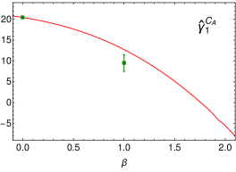
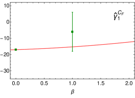
Figure 3: Two-loop soft anomalous dimension of the soft-drop jet groomer. The (green) squares with error bars represent the results of [42] — see the text.

Multi-differential soft functions: Soft functions for exclusive observables typically depend on more than one kinematic variable such that several Laplace transformations may be needed to resolve all distributions. In this case, we choose the first Laplace variable $\tau_{1}$ to have dimension 1/mass, whereas the remaining variables $\tau_{i}$ for $i\geq 2$ should be dimensionless. Our ansatz (4) for the one-emission measurement function can then be generalised to

$$\mathcal{M}_{1}(\tau_{1},\tau_{2},\ldots;k)=\exp\big{(}-\tau_{1}\,k_{T}\,y_{k}^{n/2}\,f(y_{k},t_{k};\tau_{2},\ldots)\,\big{)}\,,$$ (50)

and similarly for the two-emission functions. As long as the RGE (14) only depends on the first Laplace variable through logarithms $L_{1}=\ln(\mu\bar{\tau}_{1})$, the results from Section 3 for the soft anomalous dimension can equally be applied for multi-differential soft functions. The same is true for the expressions from Section 4 for the collinear anomaly exponent as long as the expansion in (29) only depends on $L_{1}$.

As an example of a double-differential soft function, we consider the one for exclusive Drell-Yan production from [43]. Due to rescaling invariance of the Wilson lines, the position-space soft function can only depend on $\tau_{1}=\sqrt{x_{+}x_{-}}$ and $\tau_{2}=\sqrt{x_{T}^{2}/x_{+}x_{-}}$, which play the role of a dimensionful and a dimensionless Laplace (or Fourier) variable. After rescaling $\tau_{1}\to\frac{i}{2}\tau_{1}$, the soft function is then specified by $n=-1$, $f(y_{k},t_{k};\tau_{2})=1+y_{k}-2\sqrt{y_{k}}(1-2t_{k})\tau_{2}$ and

$$F(a,b,y,t_{k},t_{l},t_{kl};\tau_{2})=1+y-2\;\sqrt{\frac{ay}{(1+ab)(a+b)}}\;\Big{(}b(1-2t_{k})+1-2t_{l}\Big{)}\tau_{2}\,.$$ (51)

As the underlying RGE only depends on logarithms of $\tau_{1}$ [43], we can apply the formulae from Section 3 to compute the soft anomalous dimension. This yields $\gamma^{S}_{0}=0$, $\gamma^{n_{f}}_{1}=224/27-4/9\,\pi^{2}$ and $\gamma^{C_{A}}_{1}=-808/27+11/9\,\pi^{2}+28\zeta_{3}$, along with $\gamma^{C_{F}}_{1}=0$ since the soft function is consistent with NAE in position space. These findings are in agreement with [43].

We next consider the double-differential hemisphere soft function that was computed to NNLO in [21, 44]. In this case, we take two Laplace transformations with respect to the hemisphere masses $M_{L}$ and $M_{R}$ and denote the respective Laplace variables by $\tau_{L}$ and $\tau_{R}$. We may then choose $\tau_{1}=\sqrt{\tau_{L}\tau_{R}}$ and $\tau_{2}=(\tau_{L}+\tau_{R})/\sqrt{\tau_{L}\tau_{R}}$, which is convenient since these variables respect the $\tau_{L}\leftrightarrow\tau_{R}$ symmetry of the soft function. More importantly, the RGE then again only depends on logarithms of $\tau_{1}$, such that the formulae from Section 3 can be used to compute the soft anomalous dimension. Without going into further details here, we find the same result as in the previous example, which is in line with the findings of [21, 44].

N-jet soft functions: The computation of soft functions that involve Wilson lines in more than two light-like directions is clearly more complicated and beyond the scope of the present paper. Still, it has been argued in [45] that the anomalous dimension of an $N$-jet soft function can be reconstructed from the information on dijet soft functions. The strategy of [45] relies on the fact that the two-loop hard anomalous dimensions are known for arbitrary processes [7] and that cross sections are invariant under a variation of the factorisation scale.

The authors of [45] illustrate this method with the hadronic event-shape variable transverse thrust. In the dijet limit, the transverse thrust distribution satisfies a hard-beam-jet-soft factorisation theorem that contains a soft function which depends on two incoming and two outgoing light-like directions [46]. By considering simpler toy processes, in which all but two of the hard QCD partons are replaced by leptons, the required jet and beam anomalous dimensions can then be extracted from known results of hard and soft (dijet) anomalous dimensions. This information is then used in a second step to determine the soft anomalous dimension of the $N$-jet observable.

The toy processes that are needed to determine the two-loop soft anomalous dimension for transverse thrust are $e^{+}e^{-}\to q\bar{q}$ and $q\bar{q}\to e^{+}e^{-}$ scattering. In the first case, the soft function falls into the pattern defined in Section 2 with $n=1$, $f(0,t_{k})=16t_{k}\bar{t}_{k}$ and

$$F_{A}(a,b,0,t_{k},t_{l},t_{kl}) =\frac{16(at_{l}\bar{t}_{l}+bt_{k}\bar{t}_{k})}{a+b}\,,$$

$$F_{B}(a,b,0,t_{k},t_{l},t_{kl}) =\frac{16(t_{l}\bar{t}_{l}+abt_{k}\bar{t}_{k})}{1+ab}\,.$$ (52)

The integral representations for the calculation of the soft anomalous dimension from Section 3 can then be evaluated numerically, giving $\gamma^{S}_{0}=0$, $\gamma^{n_{f}}_{1}=19.3954(5)$ and $\gamma^{C_{A}}_{1}=-158.276(5)$, as well as $\gamma^{C_{F}}_{1}=0$ since the soft function is consistent with NAE. The two-loop soft anomalous dimension for this (toy) observable was previously extracted via an EVENT2 fit in [46] with considerably larger uncertainties ($\gamma^{n_{f}}_{1}=18^{+2}_{-3}$, $\gamma^{C_{A}}_{1}=-148^{+20}_{-30}$).

The soft function for the second toy process turns out to be a SCET-2 observable with $n=0$, $f(y_{k},t_{k})=2c_{0}(1-|1-2t_{k}|)$ and

$$F(a,b,y,t_{k},t_{l},t_{kl}) =2c_{0}\;\sqrt{\frac{a}{(1+ab)(a+b)}}\;\big{(}b(1-|1-2t_{k}|)+1-|1-2t_{l}|\big{)}\,,$$ (53)

where $c_{0}=e^{4G/\pi}$ involves Catalan’s constant $G\simeq 0.915966$. In this case we obtain $d_{1}=0$, $d^{\,n_{f}}_{2}=-37.1743(5)$ and $d_{2}^{\,C_{A}}=208.098(3)$, whereas again $d_{2}^{\,C_{F}}=0$ because of NAE. These numbers can be compared to the calculation from [45], which quotes $d^{\,n_{f}}_{2}=-37.191(6)$ and $d_{2}^{\,C_{A}}=208.0(1)$.

As the strategy proposed in [45] is general, we conclude that our results for dijet soft functions can be used indirectly to determine soft anomalous dimensions for processes with more than two light-like directions.

7 Conclusions

We have developed a novel formalism for the calculation of two-loop soft anomalous dimensions that is relevant for processes with two hard, massless and colour-charged partons. As long as the corresponding soft function falls into the pattern defined in Section 2, the integral representations for the soft anomalous dimensions can easily be evaluated numerically, without having to perform an explicit two-loop calculation anymore. Our approach is sufficiently general to treat observables that are defined in SCET-1 and SCET-2, and we clarified the relation between the respective soft anomalous dimension and the collinear anomaly exponent.

By considering various examples, we illustrated that our setup can be applied to a large variety of dijet soft functions. In particular, we computed the two-loop soft anomalous dimension of the $e^{+}e^{-}$ angularity event shape and the soft-drop jet-grooming algorithm for the first time. Our results allow one to extend existing resummations for these observables to NNLL accuracy. In Section 6 we have furthermore shown that our formalism can be generalised to soft functions which a priori do not belong to the class defined in Section 2. This includes, in particular, jet-veto observables and soft functions that are relevant for processes with more than two jet directions.

We believe that our results will help facilitate precision resummations in both QCD and SCET in the future, and that they may be particularly useful for developing an automated resummation code. For convenience of the user, we plan to implement the integral representations from this paper in the forthcoming SoftSERVE distribution [13].

Acknowledgments: We are grateful to Thomas Becher and Bahman Dehnadi for helpful discussions and comments on the manuscript. G.B. is supported by the Deutsche Forschungsgemeinschaft (DFG) within Research Unit FOR 1873. R.R. is supported by the Swiss National Science Foundation (SNF) under grant CRSII2-160814. J.T. acknowledges research and travel funds from DESY. G.B. and R.R. thank the Munich Institute for Astro- and Particle Physics (MIAPP) of the DFG cluster of excellence ”Origin and Structure of the Universe” for hospitality and support.

Appendix A Details of the $C_{F}^{2}$ contribution

For the uncorrelated emission contribution, we find that the pole terms of the bare soft function only cancel as predicted by the RGE if the following constraint is satisfied,

$$\frac{8}{\pi}\,\int_{0}^{1}\!dt_{l}\;\,\frac{\ln^{2}f(0,t_{l})}{\sqrt{\rule{0.0pt}{9.95845pt}4t_{l}\bar{t}_{l}}}-\frac{16}{\pi^{2}}\,\int_{0}^{1}\!dt_{k}\;\,\frac{\ln f(0,t_{k})}{\sqrt{\rule{0.0pt}{9.95845pt}4t_{k}\bar{t}_{k}}}\;\int_{0}^{1}\!dt_{l}\;\,\frac{\ln f(0,t_{l})}{\sqrt{\rule{0.0pt}{9.95845pt}4t_{l}\bar{t}_{l}}}$$

$$\qquad-\frac{4}{\pi^{2}}\int_{0}^{1}\!db\int_{0}^{1}\!dt_{l}\int_{0}^{1}\!dt_{kl}\;\frac{1}{\sqrt{\rule{0.0pt}{9.95845pt}16t_{l}\bar{t}_{l}t_{kl}\bar{t}_{kl}}}\;\,\frac{\mathcal{G}_{1}(0,b,t_{l},t_{kl})}{b_{+}}\,=\,0\,,$$ (54)

where the explicit form of the function $\mathcal{G}_{1}(y,b,t_{l},t_{kl})$ was given in (23). We checked that this constraint is fulfilled for all soft functions we considered explicitly in this work, but we cannot prove that it holds in the general case.

Similarly, we find an additional contribution to the two-loop soft anomalous dimension $\gamma^{C_{F}}_{1}$ and the two-loop anomaly exponent $d^{\,C_{F}}_{2}$, which vanishes for all examples we considered, and which we conjecture to be zero in general. This contribution reads

$$\Delta\gamma^{C_{F}}_{1} =\frac{64}{n}\,\bigg{\{}\frac{4}{\pi}\,\int_{0}^{1}\!dt_{l}\;\,\frac{\ln^{3}f(0,t_{l})}{\sqrt{\rule{0.0pt}{9.95845pt}4t_{l}\bar{t}_{l}}}-\frac{2}{\pi}\,\int_{0}^{1}\!dt_{l}\;\,\frac{\ln(16t_{l}\bar{t}_{l})}{\sqrt{\rule{0.0pt}{9.95845pt}4t_{l}\bar{t}_{l}}}\;\ln^{2}f(0,t_{l})$$

$$\qquad\quad-\frac{8}{\pi^{2}}\,\int_{0}^{1}\!dt_{k}\;\,\frac{\ln f(0,t_{k})}{\sqrt{\rule{0.0pt}{9.95845pt}4t_{k}\bar{t}_{k}}}\;\int_{0}^{1}\!dt_{l}\;\,\frac{\ln f(0,t_{l})}{\sqrt{\rule{0.0pt}{9.95845pt}4t_{l}\bar{t}_{l}}}\;\ln\frac{f(0,t_{l})}{16t_{l}\bar{t}_{l}}$$

$$\qquad\quad+\frac{1}{\pi^{2}}\int_{0}^{1}\!db\int_{0}^{1}\!dt_{l}\int_{0}^{1}\!dt_{kl}\;\frac{1}{\sqrt{\rule{0.0pt}{9.95845pt}16t_{l}\bar{t}_{l}t_{kl}\bar{t}_{kl}}}\;\,\bigg{[}\frac{1}{b}\,\ln\frac{256\,t_{l}\bar{t}_{l}t_{kl}\bar{t}_{kl}\,b^{2}}{(1+b)^{4}}\bigg{]}_{+}\;\mathcal{G}_{1}(0,b,t_{l},t_{kl})$$

$$\qquad\quad-\frac{2}{\pi^{2}}\int_{0}^{1}\!db\int_{0}^{1}\!dt_{l}\int_{0}^{1}\!dt_{kl}\;\frac{1}{\sqrt{\rule{0.0pt}{9.95845pt}16t_{l}\bar{t}_{l}t_{kl}\bar{t}_{kl}}}\;\,\frac{\mathcal{G}_{3}(b,t_{l},t_{kl})}{b_{+}}$$

$$\qquad\quad+\frac{2}{\pi^{2}}\int_{0}^{1}\!db\int_{0}^{1}\!dt_{l}\int_{0}^{1}\!dt_{kl}\int_{0}^{1}\!ds\;\frac{1}{\sqrt{\rule{0.0pt}{9.95845pt}16t_{l}\bar{t}_{l}t_{kl}\bar{t}_{kl}}}\;\,\frac{1}{b}\bigg{[}\frac{1}{s\sqrt{1-s^{2}}}\bigg{]}_{+}\;\mathcal{G}_{4}(b,t_{l},t_{kl},s)\bigg{\}}$$ (55)

for the soft anomalous dimension, and

$$\Delta d^{\,C_{F}}_{2} =64\,\bigg{\{}-\frac{4}{\pi}\,\int_{0}^{1}\!dt_{l}\;\,\frac{\ln^{3}f(0,t_{l})}{\sqrt{\rule{0.0pt}{9.95845pt}4t_{l}\bar{t}_{l}}}+\frac{8}{\pi^{2}}\,\int_{0}^{1}\!dt_{k}\;\,\frac{\ln f(0,t_{k})}{\sqrt{\rule{0.0pt}{9.95845pt}4t_{k}\bar{t}_{k}}}\;\int_{0}^{1}\!dt_{l}\;\,\frac{\ln^{2}f(0,t_{l})}{\sqrt{\rule{0.0pt}{9.95845pt}4t_{l}\bar{t}_{l}}}\;$$

$$\qquad\quad-\frac{1}{\pi^{2}}\int_{0}^{1}\!db\int_{0}^{1}\!dt_{l}\int_{0}^{1}\!dt_{kl}\;\frac{1}{\sqrt{\rule{0.0pt}{9.95845pt}16t_{l}\bar{t}_{l}t_{kl}\bar{t}_{kl}}}\;\,\bigg{[}\frac{1}{b}\,\ln\frac{b^{2}}{(1+b)^{4}}\bigg{]}_{+}\;\mathcal{G}_{1}(0,b,t_{l},t_{kl})$$

$$\qquad\quad+\frac{2}{\pi^{2}}\int_{0}^{1}\!db\int_{0}^{1}\!dt_{l}\int_{0}^{1}\!dt_{kl}\;\frac{1}{\sqrt{\rule{0.0pt}{9.95845pt}16t_{l}\bar{t}_{l}t_{kl}\bar{t}_{kl}}}\;\,\frac{\mathcal{G}_{3}(b,t_{l},t_{kl})}{b_{+}}\bigg{\}}$$ (56)

for the collinear anomaly exponent. Here

$$\mathcal{G}_{3}(b,t_{l},t_{kl}) =\ln^{2}G_{A_{1}}(0,0,b,t_{k}^{+},t_{l},t_{kl})+\ln^{2}G_{A_{2}}(0,0,b,t_{k}^{+},t_{l},t_{kl})$$

$$\quad+\ln^{2}G_{B_{1}}(0,0,b,t_{k}^{+},t_{l},t_{kl})+\ln^{2}G_{B_{2}}(0,0,b,t_{k}^{+},t_{l},t_{kl})+(t_{k}^{+}\to t_{k}^{-})\,,$$

$$\mathcal{G}_{4}(b,t_{l},t_{kl},s) =\ln G_{A_{1}}(0,0,b,t_{k}^{\oplus},t_{l},t_{kl})+\ln G_{A_{2}}(0,0,b,t_{k}^{\oplus},t_{l},t_{kl})$$

$$\quad+\ln G_{B_{1}}(0,0,b,t_{k}^{\oplus},t_{l},t_{kl})+\ln G_{B_{2}}(0,0,b,t_{k}^{\oplus},t_{l},t_{kl})+(t_{k}^{\oplus}\to t_{k}^{\ominus})\,,$$ (57)

and

$$t_{k}^{\oplus} =t_{l}+t_{kl}-2t_{l}t_{kl}+2\sqrt{t_{l}\bar{t}_{l}t_{kl}\bar{t}_{kl}(1-s^{2})}\,,$$

$$t_{k}^{\ominus} =t_{l}+t_{kl}-2t_{l}t_{kl}-2\sqrt{t_{l}\bar{t}_{l}t_{kl}\bar{t}_{kl}(1-s^{2})}\,.$$ (58)

For the cumulant soft functions $\widehat{S}(\omega,\mu)$ discussed in Section 6, the above relations are slightly modified. In particular, we find an additional term $-2\pi^{2}/3$ on the left hand side of equation (54) and, similarly, the corresponding relations to (55) and (56) for cumulant soft functions become

$$\Delta\widehat{\gamma}^{C_{F}}_{1} =\Delta\gamma^{C_{F}}_{1}-\frac{256\zeta_{3}}{n}+\frac{16\pi^{2}}{3n}\,\frac{\gamma^{S}_{0}}{C_{F}}\,,$$

$$\Delta\widehat{d}^{\,C_{F}}_{2} =\Delta d^{\,C_{F}}_{2}+256\zeta_{3}+\frac{16\pi^{2}}{3}\,\frac{d_{1}}{C_{F}}\,,$$ (59)

which we again conjecture to vanish for all observables.

Appendix B Details of cumulant soft functions

In this appendix we list the explicit expressions for the measurement functions of the three cumulant soft functions discussed in Section 6. These are required to compute the soft anomalous dimensions and the collinear anomaly exponents from Figures 6 and 3.

Rapidity-dependent jet vetoes: As the four jet-veto observables from [37] have the same soft anomalous dimension, we focus here on the C-parameter jet veto in the hadronic center-of-mass frame, $\mathcal{T}_{C\rm cm}$, for concreteness. The corresponding soft function is specified by $n=1$, $f(y_{k},t_{k})=1/(1+y_{k})$ and

$$F_{A}(a,b,0,t_{k},t_{l},t_{kl}) =\theta(\Delta_{F}-R)\;\frac{\text{max}(a,b)}{a+b}+\theta(R-\Delta_{F})\,,$$

$$F_{B}(a,b,0,t_{k},t_{l},t_{kl}) =\theta(\Delta_{F}-R)\;\frac{\text{max}(1,ab)}{1+ab}+\theta(R-\Delta_{F})\,,$$ (60)

where $R$ is the jet radius and $\Delta_{F}=\sqrt{\ln^{2}a+\arccos^{2}(1-2t_{kl})}$ represents the clustering condition in the parametrisation (5). For uncorrelated emissions, we find

$$G_{i}(y,0,b,t_{k},t_{l},t_{kl}) =\frac{1}{(1+b)(1+y)}\,,\hskip 107.26688pt(i=A_{1},A_{2},B_{1},B_{2})$$

$$G_{i}(0,r,b,t_{k},t_{l},t_{kl}) =\theta(\Delta_{G}-R)\;\frac{1}{1+b}+\theta(R-\Delta_{G})\,,\qquad(i=A_{1},A_{2})$$

$$G_{i}(0,r,b,t_{k},t_{l},t_{kl}) =\frac{1}{1+b}\,,\hskip 152.79129pt(i=B_{1},B_{2})$$ (61)

where $\Delta_{G}=\sqrt{\frac{1}{4}\ln^{2}r+\arccos^{2}(1-2t_{kl})}$ is the analogous clustering constraint in the parametrisation (2).

Standard jet veto: The $p_{T}$ jet veto turns out to be a SCET-2 observable that depends on the same clustering conditions in terms of $\Delta_{F}$ and $\Delta_{G}$ as in the previous example. The corresponding soft function satisfies $n=0$, $f(y_{k},t_{k})=1$ and

$$F_{i}(a,b,0,t_{k},t_{l},t_{kl}) =\sqrt{\frac{a}{(a+b)(1+ab)}}\Big{(}\theta(\Delta_{F}-R)+\theta(R-\Delta_{F})\;\sqrt{1+b^{2}+2b(1-2t_{kl})}\Big{)}$$ (62)

for both regions $i=A,B$. For uncorrelated emissions, we now obtain

$$G_{i}(y,0,b,t_{k},t_{l},t_{kl}) =\frac{1}{1+b}\,,\hskip 182.09763pt(i=A_{1},A_{2},B_{1},B_{2})$$

$$G_{i}(0,r,b,t_{k},t_{l},t_{kl}) =\theta(\Delta_{G}-R)\;\frac{1}{1+b}$$

$$\quad+\theta(R-\Delta_{G})\;\frac{\sqrt{1+b^{2}+2b(1-2t_{kl})}}{1+b}\,,\qquad(i=A_{1},A_{2})$$

$$G_{i}(0,r,b,t_{k},t_{l},t_{kl}) =\frac{1}{1+b}\,.\hskip 181.81308pt(i=B_{1},B_{2})$$ (63)

Jet grooming: The soft function for the soft-drop jet grooming algorithm is characterised by $n=-1-\beta$, $f(y_{k},t_{k})=(1+y_{k})^{1+\beta/2}$ (for $0\leq y_{k}\leq 1$) and

$$F_{A}(a,b,0,t_{k},t_{l},t_{kl}) =1+\theta(1+4at_{kl}-2a)\,\left(a^{-\beta/2}(a+b)^{\beta/2}(1+ab)^{-1-\beta/2}-1\right)\,,$$

$$F_{B}(a,b,0,t_{k},t_{l},t_{kl}) =1+\theta(1+4at_{kl}-2a)$$

$$\qquad\Big{\{}\theta(b-a^{1+\beta})\,b\,a^{-\beta/2}(a+b)^{-1-\beta/2}(1+ab)^{\beta/2}$$

$$\qquad\quad+\theta(a^{1+\beta}-b)\,a^{1+\beta/2}(a+b)^{-1-\beta/2}(1+ab)^{\beta/2}-1\Big{\}}\,.$$ (64)

The measurement function for the uncorrelated emission contribution is in this case given by

$$G_{i}(y,0,b,t_{k},t_{l},t_{kl}) =\frac{(1+y)^{1+\beta}}{1+b}\,,\hskip 242.13297pt(i=A_{1},B_{1})$$

$$G_{i}(y,0,b,t_{k},t_{l},t_{kl}) =\theta_{1}\,\frac{(1+y)^{1+\beta/2}}{1+b}+(1-\theta_{1})\,\frac{b(1+y)^{1+\beta}}{1+b}\,,\hskip 105.27519pt(i=A_{2},B_{2})$$

$$G_{A_{1}}(0,r,b,t_{k},t_{l},t_{kl}) =\theta_{2}\theta_{3}\,\frac{(b+r^{1+\beta/2})^{-\beta/2}(b+r^{\beta/2})^{1+\beta/2}}{1+b}+(1-\theta_{2}\theta_{3})\,\frac{1}{1+b}\,,$$

$$G_{A_{2}}(0,r,b,t_{k},t_{l},t_{kl}) =\theta_{2}\theta_{3}\,\frac{(b\,r^{1+\beta/2}+1)^{-\beta/2}(b\,r^{\beta/2}+1)^{1+\beta/2}}{1+b}+(1-\theta_{2}\theta_{3})\,\frac{1}{1+b}\,,$$

$$G_{i}(0,r,b,t_{k},t_{l},t_{kl}) =\frac{1}{1+b}\,,\hskip 268.594pt(i=B_{1},B_{2})$$ (65)

where $\theta_{1}=\theta\big{(}1-b(1+y)^{\beta/2}\big{)}$, $\theta_{2}=\theta\big{(}2(1-2t_{kl})-\sqrt{r}\big{)}$ and $\theta_{3}=\theta\big{(}2\sqrt{r}(1-2t_{kl})-1\big{)}$.

References

[1]
J. C. Collins, D. E. Soper and G. F. Sterman,
Adv. Ser. Direct. High Energy Phys. 5 (1989) 1
[hep-ph/0409313].
[3]
L. G. Almeida, S. D. Ellis, C. Lee, G. Sterman, I. Sung and J. R. Walsh,
JHEP 1404 (2014) 174
[arXiv:1401.4460 [hep-ph]].
[4]
C. W. Bauer, S. Fleming, D. Pirjol and I. W. Stewart,
Phys. Rev. D 63 (2001) 114020
[hep-ph/0011336].
[5]
C. W. Bauer, D. Pirjol and I. W. Stewart,
Phys. Rev. D 65 (2002) 054022
[hep-ph/0109045].
[6]
M. Beneke, A. P. Chapovsky, M. Diehl and T. Feldmann,
Nucl. Phys. B 643 (2002) 431
[hep-ph/0206152].
[7]
T. Becher and M. Neubert,
JHEP 0906 (2009) 081
Erratum: [JHEP 1311 (2013) 024]
[arXiv:0903.1126 [hep-ph]].
[8]
S. Catani and M. Grazzini,
Nucl. Phys. B 591 (2000) 435
[hep-ph/0007142].
[9]
D. Kang, O. Z. Labun and C. Lee,
Phys. Lett. B 748 (2015) 45
[arXiv:1504.04006 [hep-ph]].
[10]
T. Becher and M. Neubert,
Eur. Phys. J. C 71 (2011) 1665
[arXiv:1007.4005 [hep-ph]].
[11]
J. Y. Chiu, A. Jain, D. Neill and I. Z. Rothstein,
JHEP 1205 (2012) 084
[arXiv:1202.0814 [hep-ph]].
[12]
T. Becher and G. Bell,
Phys. Lett. B 713 (2012) 41
[arXiv:1112.3907 [hep-ph]].
[13]
G. Bell, R. Rahn and J. Talbert,
arXiv:1812.08690 [hep-ph].
[14]
G. Bell, R. Rahn and J. Talbert,
PoS RADCOR 2015 (2016) 052
[arXiv:1512.06100 [hep-ph]].
[15]
G. Bell, R. Rahn and J. Talbert,
PoS RADCOR 2017 (2018) 047
[arXiv:1801.04877 [hep-ph]].
[16]
T. Becher, G. Bell and S. Marti,
JHEP 1204 (2012) 034
[arXiv:1201.5572 [hep-ph]].
[17]
J. G. M. Gatheral,
Phys. Lett. 133B (1983) 90.
[18]
J. Frenkel and J. C. Taylor,
Nucl. Phys. B 246 (1984) 231.
[19]
A. V. Belitsky,
Phys. Lett. B 442 (1998) 307
[hep-ph/9808389].
[20]
T. Becher, M. Neubert and G. Xu,
JHEP 0807 (2008) 030
[arXiv:0710.0680 [hep-ph]].
[21]
R. Kelley, M. D. Schwartz, R. M. Schabinger and H. X. Zhu,
Phys. Rev. D 84 (2011) 045022
[arXiv:1105.3676 [hep-ph]].
[22]
P. F. Monni, T. Gehrmann and G. Luisoni,
JHEP 1108 (2011) 010
[arXiv:1105.4560 [hep-ph]].
[23]
A. H. Hoang, D. W. Kolodrubetz, V. Mateu and I. W. Stewart,
Phys. Rev. D 91 (2015) no.9, 094017
[arXiv:1411.6633 [hep-ph]].
[24]
C. F. Berger, T. Kucs and G. F. Sterman,
Phys. Rev. D 68 (2003) 014012
[hep-ph/0303051].
[25]
A. Hornig, C. Lee and G. Ovanesyan,
JHEP 0905 (2009) 122
[arXiv:0901.3780 [hep-ph]].
[26]
G. Bell, A. Hornig, C. Lee and J. Talbert,
in Proceedings to ”Parton Radiation and Fragmentation from LHC to FCC-ee”,
CERN, Geneva, Switzerland, November 22-23, 2016,
pp. 90-96, 2017.
[27]
M. Procura, W. J. Waalewijn and L. Zeune,
JHEP 1810 (2018) 098
[arXiv:1806.10622 [hep-ph]].
[28]
G. Bell, A. Hornig, C. Lee and J. Talbert,
JHEP 1901 (2019) 147
[arXiv:1808.07867 [hep-ph]].
[29]
A. J. Larkoski, D. Neill and J. Thaler,
JHEP 1404 (2014) 017
[arXiv:1401.2158 [hep-ph]].
[30]
T. Becher and G. Bell,
JHEP 1211 (2012) 126
[arXiv:1210.0580 [hep-ph]].
[31]
M. G. Echevarria, I. Scimemi and A. Vladimirov,
Phys. Rev. D 93 (2016) no.5, 054004
[arXiv:1511.05590 [hep-ph]].
[32]
T. Luebbert, J. Oredsson and M. Stahlhofen,
JHEP 1603 (2016) 168
[arXiv:1602.01829 [hep-ph]].
[33]
T. Gehrmann, T. Luebbert and L. L. Yang,
JHEP 1406 (2014) 155
[arXiv:1403.6451 [hep-ph]].
[34]
T. Becher, G. Bell and M. Neubert,
Phys. Lett. B 704 (2011) 276
[arXiv:1104.4108 [hep-ph]].
[35]
Y. Li and H. X. Zhu,
Phys. Rev. Lett. 118 (2017) no.2, 022004
[arXiv:1604.01404 [hep-ph]].
[36]
A. A. Vladimirov,
Phys. Rev. Lett. 118 (2017) no.6, 062001
[arXiv:1610.05791 [hep-ph]].
[37]
S. Gangal, M. Stahlhofen and F. J. Tackmann,
Phys. Rev. D 91 (2015) no.5, 054023
[arXiv:1412.4792 [hep-ph]].
[38]
T. Becher, M. Neubert and L. Rothen,
JHEP 1310 (2013) 125
[arXiv:1307.0025 [hep-ph]].
[39]
I. W. Stewart, F. J. Tackmann, J. R. Walsh and S. Zuberi,
Phys. Rev. D 89 (2014) no.5, 054001
[arXiv:1307.1808 [hep-ph]].
[40]
S. Gangal, J. R. Gaunt, M. Stahlhofen and F. J. Tackmann,
JHEP 1702 (2017) 026
[arXiv:1608.01999 [hep-ph]].
[41]
A. Banfi, G. P. Salam and G. Zanderighi,
JHEP 1206 (2012) 159
[arXiv:1203.5773 [hep-ph]].
[42]
C. Frye, A. J. Larkoski, M. D. Schwartz and K. Yan,
JHEP 1607 (2016) 064
[arXiv:1603.09338 [hep-ph]].
[43]
Y. Li, S. Mantry and F. Petriello,
Phys. Rev. D 84 (2011) 094014
[arXiv:1105.5171 [hep-ph]].
[44]
A. Hornig, C. Lee, I. W. Stewart, J. R. Walsh and S. Zuberi,
JHEP 1108 (2011) 054
Erratum: [JHEP 1710 (2017) 101]
[arXiv:1105.4628 [hep-ph]].
[45]
T. Becher, X. Garcia i Tormo and J. Piclum,
Phys. Rev. D 93 (2016) no.5, 054038
Erratum: [Phys. Rev. D 93 (2016) no.7, 079905]
[arXiv:1512.00022 [hep-ph]].
[46]
T. Becher and X. Garcia i Tormo,
JHEP 1506 (2015) 071
[arXiv:1502.04136 [hep-ph]].