Towards an algebraic method of solar cycle prediction

Abstract

An algebraic method for the reconstruction and potentially prediction of the solar dipole moment value at sunspot minimum (known to be a good predictor of the amplitude of the next solar cycle) was suggested in the first paper in this series. The method sums up the ultimate dipole moment contributions of individual active regions in a solar cycle: for this, detailed and reliable input data would in principle be needed for thousands of active regions in a solar cycle. To reduce the need for detailed input data, here we propose a new active region descriptor called ARDoR (Active Region Degree of Rogueness). In a detailed statistical analysis of a large number of activity cycles simulated with the 2$\times$2D dynamo model we demonstrate that ranking active regions by decreasing ARDoR, for a good reproduction of the solar dipole moment at the end of the cycle it is sufficient to consider the top $N$ regions on this list explicitly, where $N$ is a relatively low number, while for the other regions the ARDoR value may be set to zero. E.g., with $N=5$ the fraction of cycles where the dipole moment is reproduced with an error exceeding $\pm 30$ % is only 12%, significantly reduced with respect to the case $N=0$, i.e. ARDoR set to zero for all active regions, where this fraction is 26%. This indicates that stochastic effects on the intercycle variations of solar activity are dominated by the effect of a low number of large “rogue” active regions, rather than the combined effect of numerous small ARs. The method has a potential for future use in solar cycle prediction.

1 General introduction

The magnetic fields responsible for solar activity phenomena emerge into the solar atmosphere in a concentrated form, in active regions (ARs). In each solar cycle thousands of active regions are listed in the official NOAA database and many more small active regions are missed if their heliographic position and lifetime do not render them directly observable on the visible hemisphere. Similarly, no detailed catalogues exist for the ubiquitous ephemeral active regions, of even smaller size.

The emergence of this large number of (typically) bipolar magnetic regions obeys some well known statistical regularities like Hale’s polarity rules and Joy’s law. As a consequence, upon their decay by turbulent diffusion their remains contribute to the large-scale ordered photospheric magnetic field, including the Sun’s global axial dipole field (the so-called Babcock–Leighton mechanism). Active regions emerging in a given solar cycle contribute on average to the global dipole with a sign opposite to the preexisting field at the start of the cycle, and these contributions from active regions add up until, some time in the middle of the cycle, the global field reverses and a new cycle starts at the Sun’s poles, still overlapping with the ongoing cycle at low latitudes. Flux emergence is thus an important element of the solar dynamo mechanism sustaining the periodically overturning solar magnetic field.

The inherently stochastic nature of flux emergence introduces random fluctuations into this statistically ordered process. In recent years it has been realized that the random nature of flux emergence can give rise to significant deviations of the solar dipole moment built up during a cycle from its expected mean value: in some cycles a small number of so-called “rogue” active regions (Petrovay and Nagy 2018) with atypical properties may lead to a major, unexpected change in the level of activity. The unexpected change in the level of activity from solar cycle 23 to 24 has been interpreted as the result a few such abnormal regions by Jiang et al. (2015), while in a dynamo model Nagy et al. (2017) found that in extreme cases even a single rogue AR can trigger a grand minimum.

An open question is how to identify the [candidate] rogue active regions, and how many such regions need to be considered in individual detail in models aiming to reproduce the evolution of the Sun’s large scale field. It is not a priori clear that this number is low, so the question we pose in this paper is whether the stochastic effects in cycle-to-cycle variation originating in the random nature of the flux emergence process are dominated by a few “rogue” AR in each cycle with individually large and unusual contributions to the dipole moment, or by the “fluctuation background” due to numerous other AR with individually much lower deviations from the expected dipole contribution. While the recent studies cited above stressed the importance of a few large rogue AR, the importance of the fluctuation background cannot be discarded out of hand. The issue has obvious practical significance from the point of view of solar cycle prediction: it would be useful to know how many (and exactly which) observed individual AR need to be assimilated into a model for successful forecasts.

A related investigation was recently carried out by Whitbread et al. (2018). In that work ARs were ordered by their individual contributions to the global axial dipole moment: it was found that, far from being dominated by a few ARs with the largest contributions, the global dipole moment built up during a cycle cannot be reproduced without taking into account a large number (hundreds) of ARs. In another recent work Cameron and Schüssler (2020) found that even ephemeral active regions contribute to the net toroidal flux loss from the Sun by an amount comparable to the contribution of large active regions. By analogy, this opens the possibility that ephemeral ARs may also contribute to the global poloidal field by a non-negligible amount, though statistical studies of the orientation of ephemeral ARs are unfortunately rare (cf. Tlatov et al. 2010).

While these interesting results shed new light on the overall role of flux emergence in smaller bipoles in the global dynamo, we think that from the point of view of solar cycle prediction, instead of the dipole moment contribution per se, a more relevant control parameter is the deviation of the dipole contribution from the case with no random fluctations in flux emergence, i.e. the “degree of rogueness” (DoR). We therefore set out to systematically study the effect of individual AR on the subsequent course of solar activity using the DoR as an ordering parameter.

The question immediately arises how this DoR should be defined.

The approach we take in this work assumes that the effect of random fluctuations manifests itself primarily in the properties of individual active regions, rather than in their spatiotemporal distribution. The DoR based on individual AR properties will be called “active region degree of rogueness” — ARDoR for brevity.

The structure of this paper is as follows. Section 2 introduces and discusses our definition of ARDoR. In Section 3, after recalling salient features of the 2$\times$2D dynamo model, we use statistics based on this model to answer the central question of this paper. Conclusions are drawn in Section 4.

2 Introducing ARDoR

The Sun’s axial dipolar moment is expressed as

$$D(t)=\frac{3}{2}\int_{-\pi/2}^{\pi/2}B(\lambda,t)\sin\lambda\cos\lambda\,\mathrm{d}\lambda,$$ (1)

where $B$ is the azimuthal average of the large scale photospheric magnetic field (assumed to be radial) while $\lambda$ is heliographic latitude.

The value $D_{n}$ of this dipole moment at the start of cycle $n$ is widely considered the best physics-based precursor of the the amplitude of the incipient cyle $n$ (Petrovay 2020). Understanding intercycle variations in solar activity and potentially extending the scope of the prediction calls for an effective and robust method to compute $D_{n}$ from (often limited) observational data on the previous course of solar activity.

In the first paper of this series, Petrovay et al. (2020) (hereafter Paper 1) we suggested a simplified approach to the computation of the evolution of the global axial dipole moment of the Sun. Instead of solving the partial differential equation normally used for modeling surface magnetic flux transport (SFT) processes on the Sun, this method simply represents the dipole moment by an algebraic sum:

$$\Delta D_{n}\equiv D_{n+1}-D_{n}=\sum_{i=1}^{N_{\mathrm{tot}}}\delta D_{U,i}=\sum_{i=1}^{N_{\mathrm{tot}}}\delta D_{\infty,i}\,e^{{(t_{i}-t_{n+1})}/\tau}=\sum_{i=1}^{N_{\mathrm{tot}}}{f_{\infty,i}}\,\delta D_{1,i}\,e^{{(t_{i}-t_{n+1})}/\tau},$$ (2)

where $i$ indexes the active regions in a cycle, $N_{\mathrm{tot}}$ is the total number of ARs in the cycle, $\delta D_{1}$ is the initial contribution of an active region to the global dipole moment, $\delta D_{U}$ is its ultimate contribution at the end of a cycle and $\tau\leq\infty$ is the assumed timescale of magnetic field decay due to radial diffusion. Furthermore,

$$f_{\infty}=\delta D_{\infty}/\delta D_{1},$$ (3)

where $\delta D_{\infty}$ is the asymptotic contribution of the same AR in a SFT model with $\tau=\infty$, once the meridional flow has concentrated the relic magnetic flux from the AR to two opposite polarity patches at the two poles. (See Paper 1 for further explanations.)

In this approach, ARs are assumed to be represented by simple bipoles at the time of their introduction into the model so their initial dipole moment contribution is given by

$$\delta D_{1}=\frac{3}{4\pi R^{2}}\,\Phi\,d_{\lambda}\cos\lambda_{0},$$ (4)

where $\Phi$ is the magnetic flux in the northern polarity patch, $d_{\lambda}$ is the latitudinal separation of the polarities, $\lambda_{0}$ is the initial latitude of [the center of] the bipole and $R$ is the radius of the Sun. As demonstrated in Paper 1, $f_{\infty}$, is in turn given by

$$f_{\infty}=\frac{a}{\lambda_{R}}\exp\left(\frac{-\lambda_{0}^{2}}{2\lambda_{R}^{2}}\right).$$ (5)

It was numerically demonstrated in Paper 1 that this Gaussian form holds quite generally irrespective of the details of the SFT model, its parameters ($\lambda_{R}$ and $a$) only have a very weak dependence on the assumed form of the meridional flow profile (at least for profiles that are closer to observations), and their value only depends on a single combination of SFT model parameters. The values of $\lambda_{R}$ and $a$ for a given SFT model may be determined by interpolation of the numerical results, as presented in Paper 1.

The terms of the sum (2) represent the ultimate dipole contributions $\delta D_{U}$ of individual active regions in a cycle at the solar minimum ending that cycle. In principle each and every active region should be represented by an explicit term in the sum. Such a case was indeed considered in Paper 1 in a comparison with a run result from the 2$\times$2D dynamo and it was found that the algebraic method returns the total change in dipole moment during a cycle quite accurately in the overwhelming majority of cycles.

When it comes to applying the method to the real Sun, however, the need to include each bipolar region in the source becomes quite a nuisance. As discussed above in the Introduction, data for individual active regions are often missing for the smaller ARs, while in the case of the larger, more complex AR representing them by an instantaneously introduced bipole is nontrivial. As it was recently pointed out by Iijima et al. (2019), for an AR with zero tilt but different extents of the two polarity distributions $\delta D_{\infty}$ will be nonzero, even though $\delta D_{1}=0$ for this configuration. The reason is that the configuration has a nonzero quadrupole moment, which may alternatively be represented by not one but two oppositely oriented dipoles slightly shifted in latitude.

Such intricacies would certainly make it advisable to keep the number of active regions explicitly represented in the sum (2) to a minimum. This again brings us to the central question of this paper: how many and which active regions need to be explicitly taken into consideration for the calculation of the solar dipole moment? While the previous study of Whitbread et al. (2018) has shown that keeping only a few ARs in the summation is certainly not correct, representing the rest of the ARs in a less faithful or detailed manner may still be admissible as long as this does not distort the statistics.

To select those few ARs that still need to be realistically represented we introduce the concept of ARDoR. As known examples of rogue AR presented e.g. in Nagy et al. (2017) are primarily rogue on account of their unusual tilts and large separations, the first idea is to define ARDoR as the difference between the ultimate dipole moment contribution of an AR and the value this would take with no scatter in the tilt and separation (i.e. if the tilt and separation were to take their expected values for the given latitude and magnetic flux, as given by eqs. (15) and (16a) in Lemerle et al. 2015).

In the present paper we thus consider the case where for the majority of ARs only the information regarding their size (magnetic flux) and heliographic latitude is retained, while further details such as polarity separation or tilt angle (and therefore $\delta D_{1}$) are simply set to their expected values for the ARs with the given flux and heliographic latitude (“reduced stochasticity” or RS representation), and compare this with the case when the actual polarity separations and tilts are used (“fully stochastic” or FS case). The active region degree of rogueness is defined by

$$\mbox{\sl ARDoR}=\delta D_{U,\mathrm{FS}}-\delta D_{U,\mathrm{RS}}=f_{\infty}\,e^{(t_{i}-t_{n+1})/\tau}(\delta D_{1,\mathrm{FS}}-\delta D_{1,\mathrm{RS}}).$$ (6)

An objection to this definition may be raised as a large AR with unusually low separation and/or tilt will yield a negligible contribution to the dipole moment ($\delta D_{U}=0$), yet it may be characterized by a large negative DoR value according to the proposed definition. On the other hand, this is arguably not a shortcoming of the approach: on the contrary, as the total flux emerging in a cycle of a given amplitude is more or less fixed, the emergence of a large AR with unusually low $\delta D_{U}$ implies that the expected $\delta D_{U}$ contribution will be “missing” at the final account, resulting in the buildup of lower-than-expected global dipole moment at the end of the cycle.

Ranking the ARs in a cycle according to their decreasing ARDoR values, we now set out to compare the results where ARDoR is explicitly considered for the top $N$ ARs on this list, while the rest of the ARs are represented in the RS approach. We ask the question what is the lowest value for $N$ for which the algebraic method still yields acceptable results?

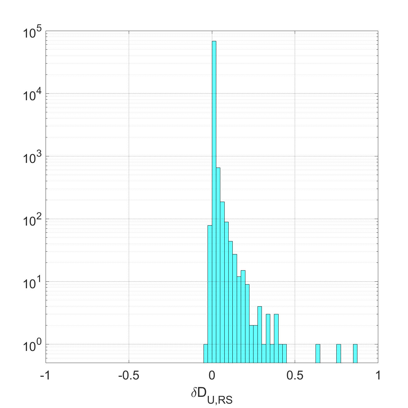
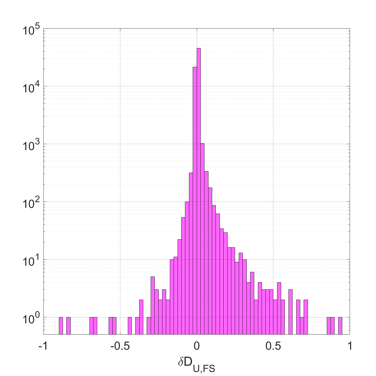
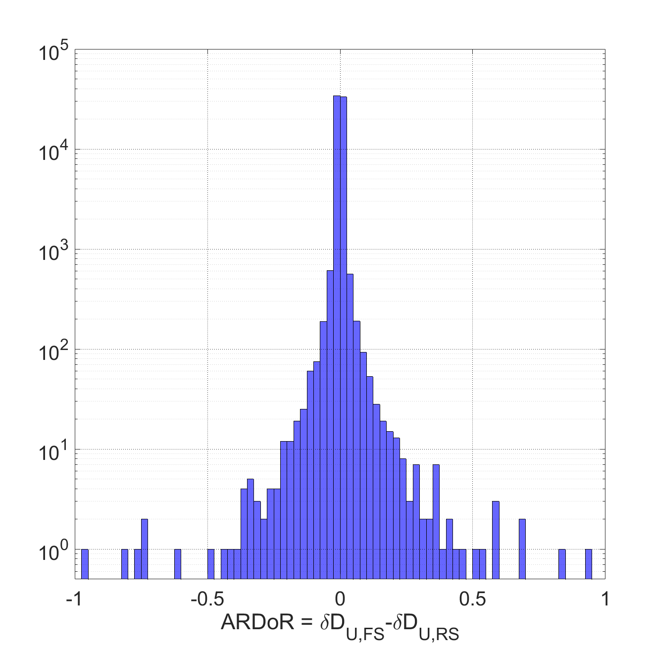
Figure 1: Histograms of ultimate dipole moment contributions of individual active regions in the FS and RS cases and their differences (i.e. ARDoR values) measured in Gauss, based on 647 cycles with an average of 3073 active regions per cycle.

N	mean	median	st.dev.
1	0.4977	0.4565	0.4146
2	0.6184	0.6022	0.4305
3	0.6696	0.6735	0.4065
4	0.6996	0.7188	0.3953
5	0.7245	0.7490	0.3535
10	0.8139	0.8078	0.3136
20	0.8838	0.8822	0.2576
50	0.9381	0.9472	0.1917
100	0.9689	0.9816	0.1324

Table 1: Means, medians and standard deviations of the total ARDoR of the top $N$ ARs divided by the total ARDoR of all ARs for cycles where the total ARDoR exceeds 15 % of the absolute change in the dipole moment $\Delta D$ (230 cycles)

3 ARDoR and rogue active regions in the 2$\times$2D dynamo model

Characteristics of the hybrid kinematic $2\times 2$D Babcock-Leighton dynamo model developed by Lemerle et al. (2015) and Lemerle and Charbonneau (2017) are particularly suitable for a study of this type. This model couples an internal axially symmetric flux transport dynamo (FTD) with a surface flux transport (SFT) model. The FTD component module provides the new active region emergences acting as a source term in the SFT component, while the output of the SFT model is used as upper boundary condition on the FTD model. In the model, bipolar magnetic regions (BMRs) representing active regions are generated at the surface randomly, with a probability based on the amplitude of the toroidal field in the deep convective zone, their properties being drawn from a statistical ensemble constructed to obey observationally determined statistical relationships. This makes it straightforward to extract the set of AR properties for any cycle from the model and to convert it to a reduced stochasticity set by setting the random fluctuations around the mean in the distributions of polarity separations and tilts to zero. In addition, the numerical efficiency of the model allows to run it for a large number of simulated solar cycles, rendering it suitable for statistical analysis of the results.

For the present analysis we use run results from the standard setup of the 2$\times$2D model as described in Lemerle and Charbonneau (2017). Evaluating the parameters of the algebraic model from the numerical results presented in Paper 1 (for the same meridional flow and parameter values as in the dynamo model) yields $\lambda_{R}=13{\hbox{$.\!\!^{\circ}$}}6$ and $a/\lambda_{R}=3.75$, so for the algebraic method these values are used. The number of simulated cycles used in the analysis was 647. The distribution of computed ARDoR values is plotted in Fig. 1.

ARs in each cycle are ranked by the ARDoR values. In each cyle we compute the absolute change $\Delta D$ in the global solar dipole moment from equation (2) for a “cocktail” of ARs, taking the ARs with the top $N$ highest ARDoR from the original, fully stochastic set, while taking the rest from the RS set. For brevity, this will be referred to as the “rank-$N$ ARDoR method”. The dipole moment change calculated with the rank-$N$ ARDoR method is then

$$\Delta D_{\mbox{\sl ARDoR},N}=\Delta D_{\mathrm{RS}}+\sum_{i=1}^{N}\mbox{\sl ARDoR}_{i}$$ (7)

where the AR index $i$ is in the order of decreasing ARDoR.

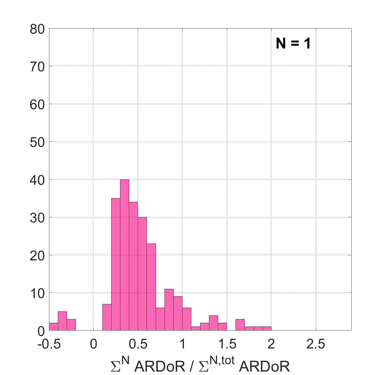
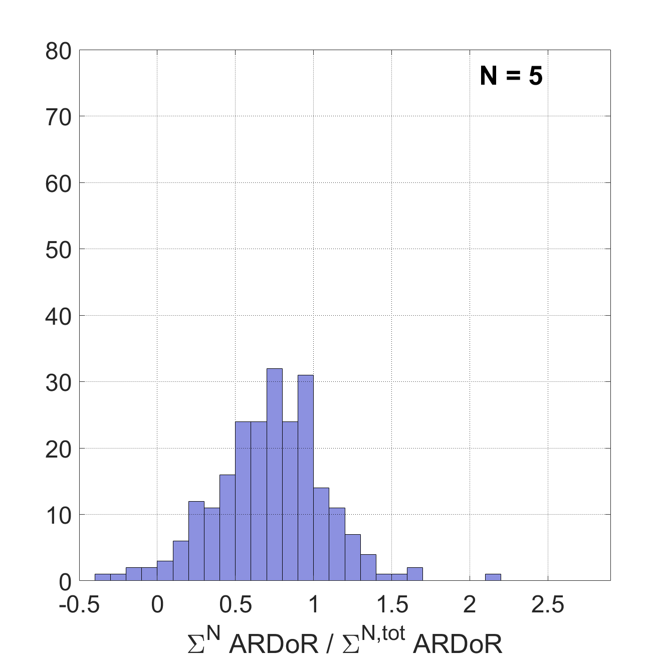
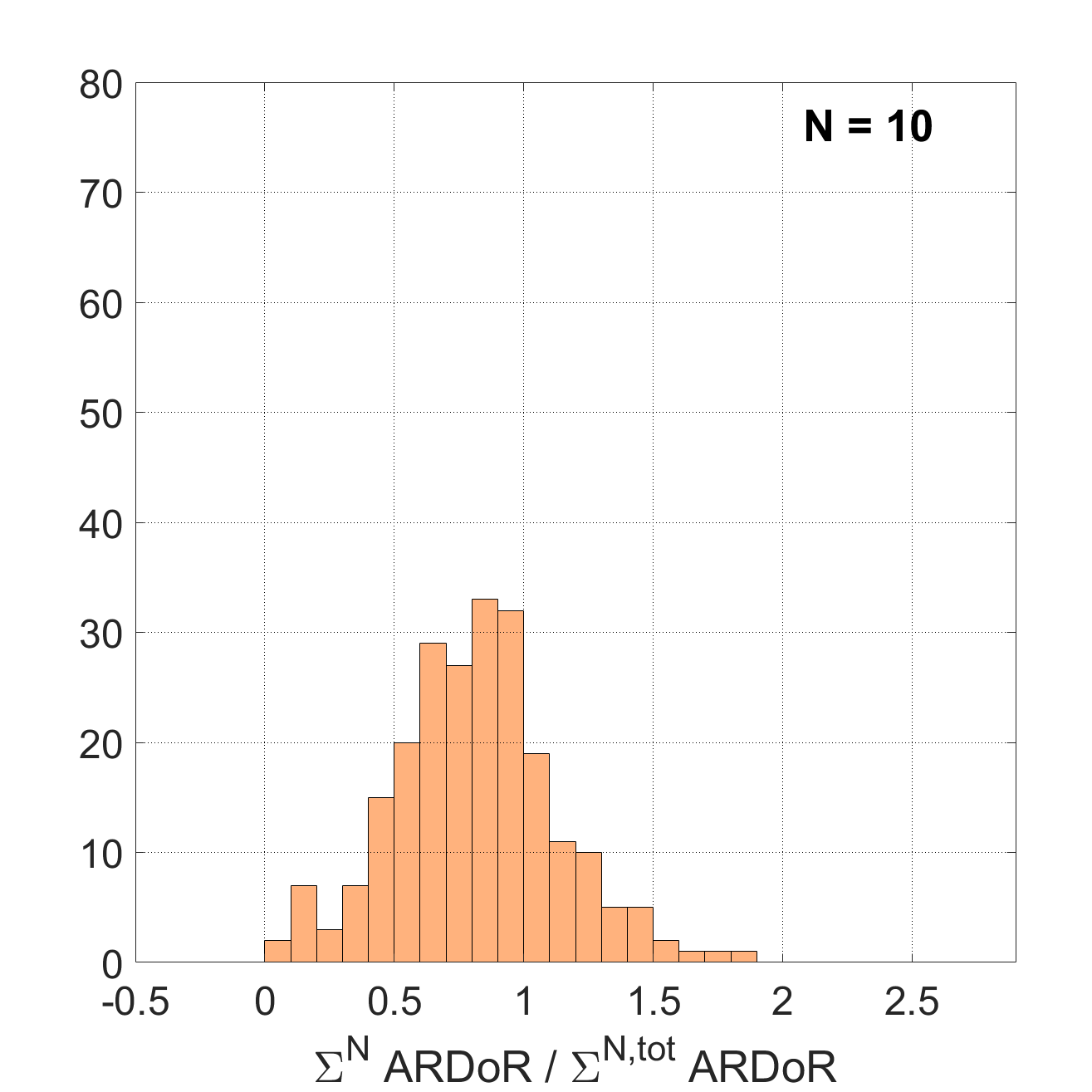
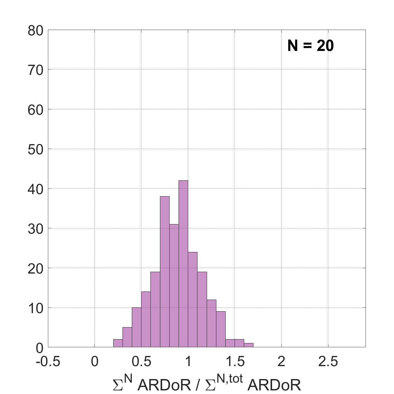
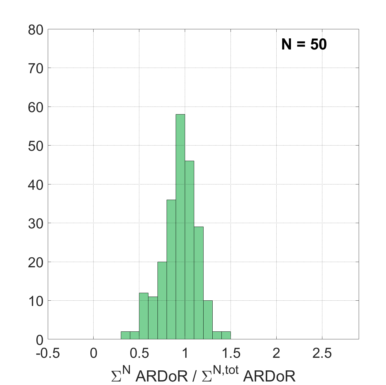
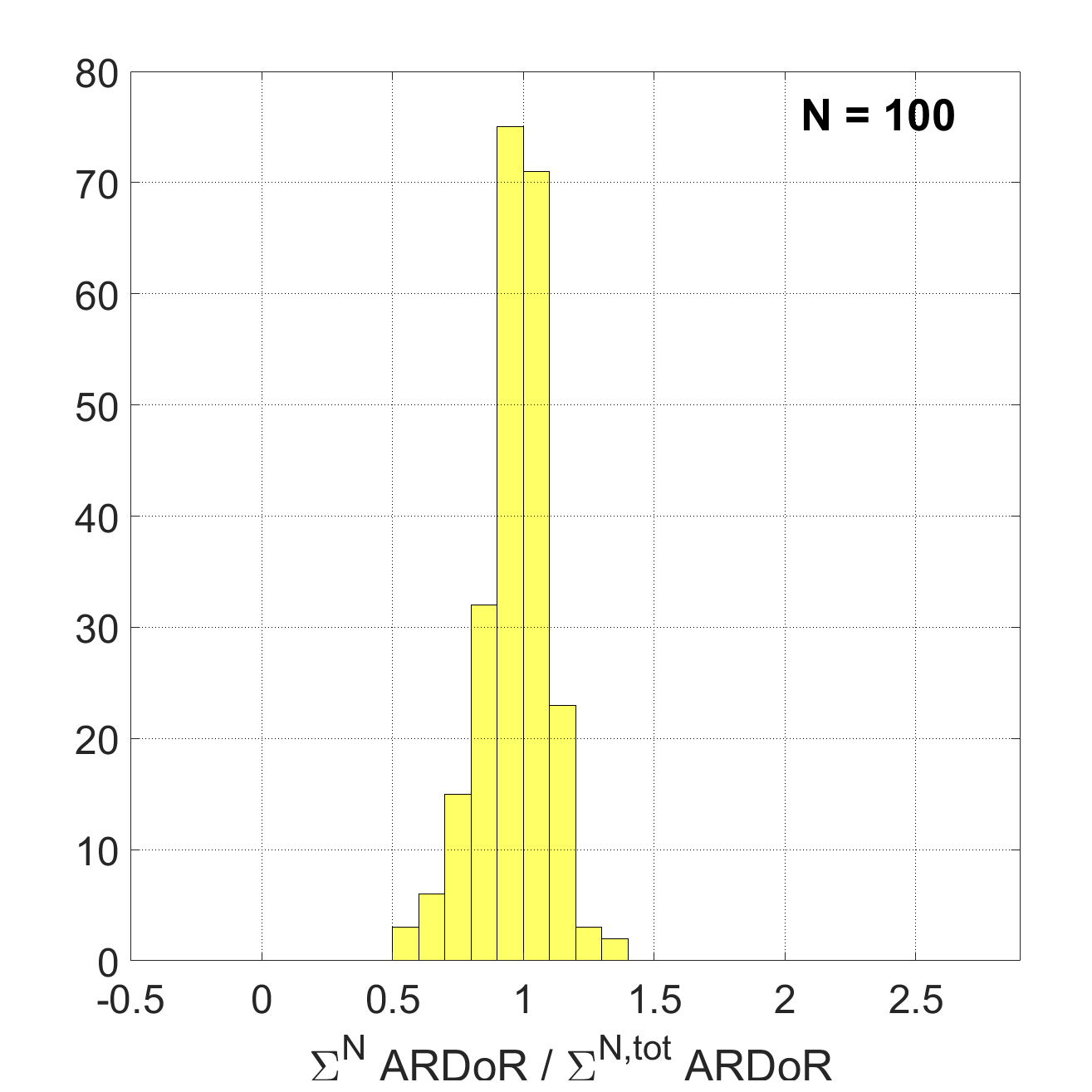
Figure 2: Histograms of the total ARDoR of the top $N$ ARs divided by the total ARDoR of all ARs for cycles where the total ARDoR exceeds 15 % of the absolute change in the dipole moment $\Delta D$ (230 cycles). The value of $N$ is shown inside each panel.

Note that the special case $N=0$, i.e. the RS set was already considered in Paper 1 where we found that even this method yields $\Delta D$ values in good agreement with the full simulations for a large majority of the cycles, but the prediction breaks down for a significant minority. As we are primarily interested in improving predictions for this minority, we first select cycles where the difference between the $\Delta D$ values from the fully stochastic and reduced stochasticity sets exceeds $\pm 15\,$%. (Note that this difference is by definition equal to the sum of ARDoRs for all ARs in the cycle, so the condition for selection was $(\sum_{i=1}^{N_{\mathrm{tot}}}\mathrm{ARDoR}_{i})/\Delta D>0.15$, which held for 230 cycles.)

Figure 2 presents histograms of the fraction of the deviation explained by ARs with the the top $N$ highest ARDoR values. Means, medians and standard deviations of these plots are collected in Table 1. It is apparent that ARs with the top 10–20 highest ARDoR are sufficient to explain 80–90 % of the deviation of $\Delta D$ computed with the reduced stochasticity model from the full value of $\Delta D$. Even the single AR with the highest ARDoR alone can explain 50 % of the deviation. Meanwhile, a significant scatter is present in the plots: e.g., adding up the columns below 0.5 and above 1.5 in the 4th panel one finds that in $\sim 8\,$% of these 230 deviating cycles even the rank-20 ARDoR method is insufficient to reproduce the deviation at an accuracy better than $\pm 50$ %. (This is $\pm 50$% of the deviation: as in this sample the mean deviation is roughly $\sim 20$% of the expected value of $\Delta D$, $\Delta D$ itself is still reproduced with an accuracy up to $\pm 10$% for these cycles.)

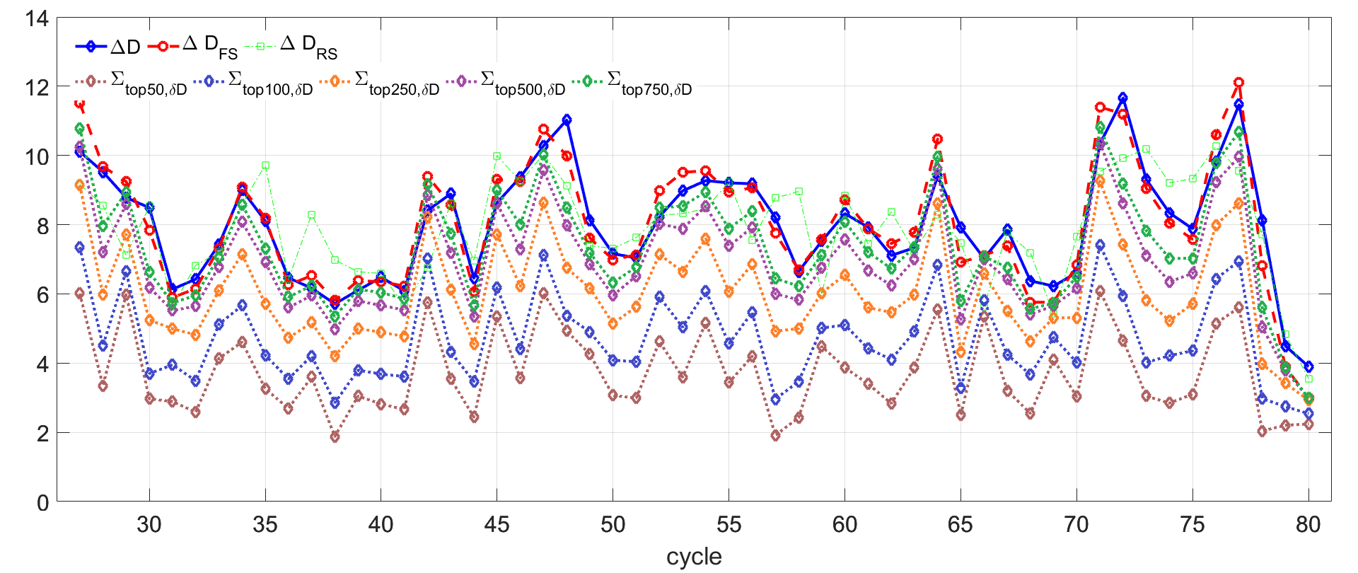
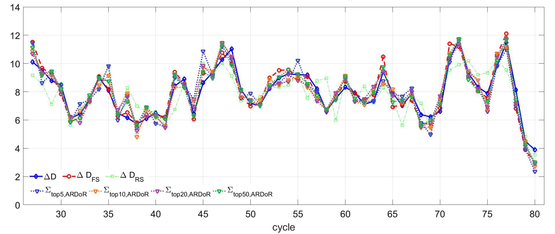
Figure 3: Absolute change $\Delta D$ on the global dipole moment during a cycle (blue solid); its approximation using the fully stochastic algebraic method (red dashed) and the reduced stochasticity algebraic method (light green dashed). The curves are compared with the absolute change computed with the algebraic method for various sets of the active regions in a cycle. Top panel: subsets containing ARs with the top $N$ highest ultimate dipole contribution (FS case). Bottom panel: subsets containing ARs with the top $N$ highest $ARDoR$ values added to $\Delta D_{\mathrm{RS}}$.

$\Delta D_{N}=\Delta D_{\mathrm{RS}}+\sum_{i=1}^{N}\mbox{\sl ARDoR}_{i}$, ranking by ARDoR:
$N$	mean	median	st.dev.	st.dev. of $(\Delta D_{N}-\Delta D)/\Delta D$
0	0.0578	0.0966	1.1365	0.212
5	–0.0115	0.0073	0.7360	0.128
10	–0.0330	–0.0116	0.7134	0.120
20	–0.0368	–0.0144	0.6662	0.125
50	–0.0599	–0.0406	0.6132	0.110
$N_{\mathrm{tot}}$	–0.0499	–0.1817	0.5861	0.101
$\sum_{i=1}^{N}\delta D_{U,i}$, ranking by $\delta_{U}$:
$N$	mean	median	st.dev.
50	4.1280	4.1777	1.4684
100	3.1874	3.1173	1.3479
250	1.8958	1.7491	1.1311
500	1.0129	0.8471	0.9346
750	0.6003	0.4895	0.8186

Table 2: Means, medians and standard deviations of the residuals of various approximations relative to the simulated value of the absolute dipole moment change $\Delta D$ during an activity cycle, as plotted in Fig. 3.

The improvement that the ARDoR method brings to the problem of reproducing the solar axial dipole moment at the end of a cycle is dramatically illustrated in Fig. 3. While in the case of ranking ARs by $\delta D$ even adding contributions from the top 750 AR yields only a barely tolerable representation of the dipole moment variation, the ARDoR method produces excellent agreement already for very low values of the rank $N$. The quality of these representations is documented in Table 2. The standard deviation of the rank-5 ARDoR method relative to the simulation result is lower than in the case of $\Delta D$ calculated from even the top 750 highest $\delta D$ contributions.

Finally, in Fig. 4 we present histograms of the deviations from the simulated value of $\Delta D$ computed with the various methods (FS, RS and ARDoR with different $N$ values). Here deviations are expressed as fractions of the actual $\Delta D$ resulting from the simulations, i.e. the quantities given in the headings of Table 2 are divided by $\Delta D$. Adding up the columns it is straightforward to work out from this that, e.g., in the case of the rank-5 ARDoR method (i.e., considering only the top 5 highest ARDoR values and adding them to the RS algebraic result), the deviation of $\Delta D$ from the simulated cycle change in the global dipole moment is less than 15 % in 88 % of the cycles. As $\Delta D$ is, on average, twice the amplitude of the polar field at minimum, the rank-5 ARDoR method reproduces the polar field precursor within $\pm 30$ % in 88 % of all cycles. This is to be compared to 74 % of the cycles in the RS case.

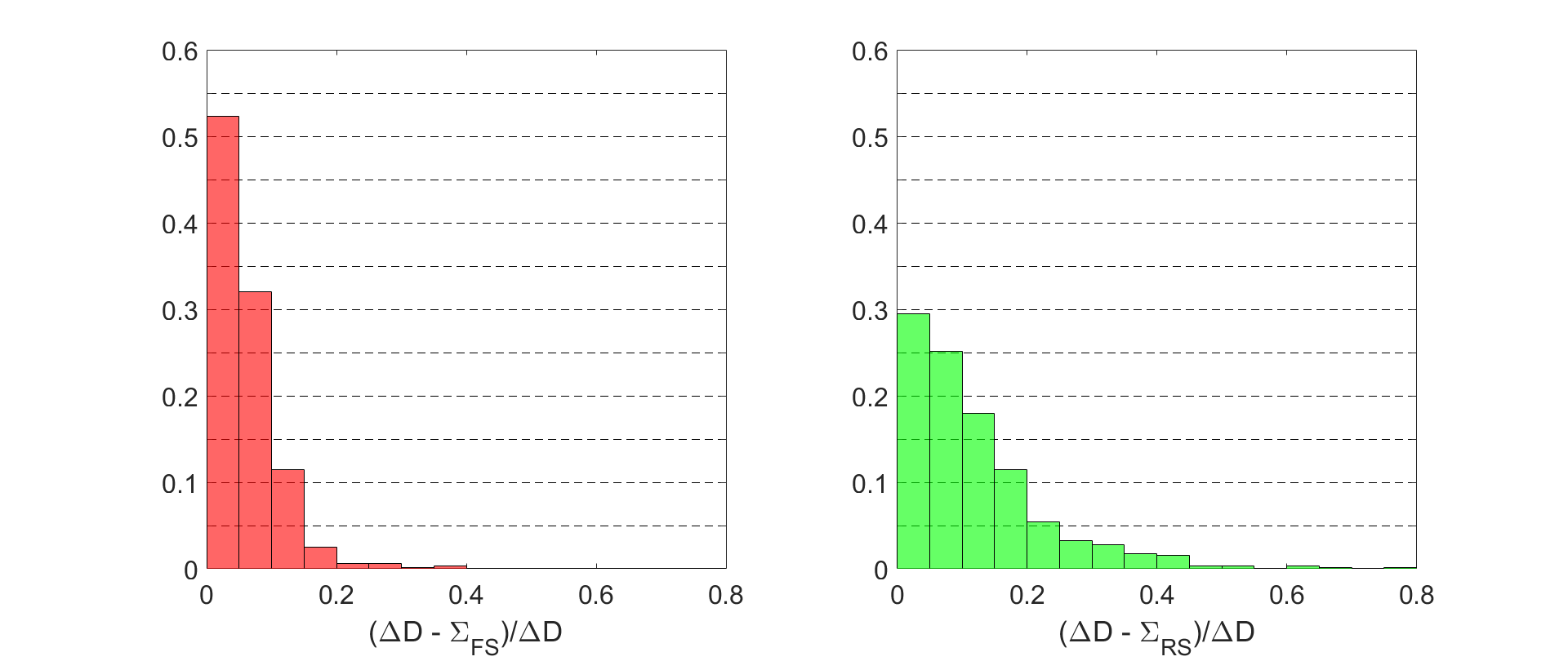
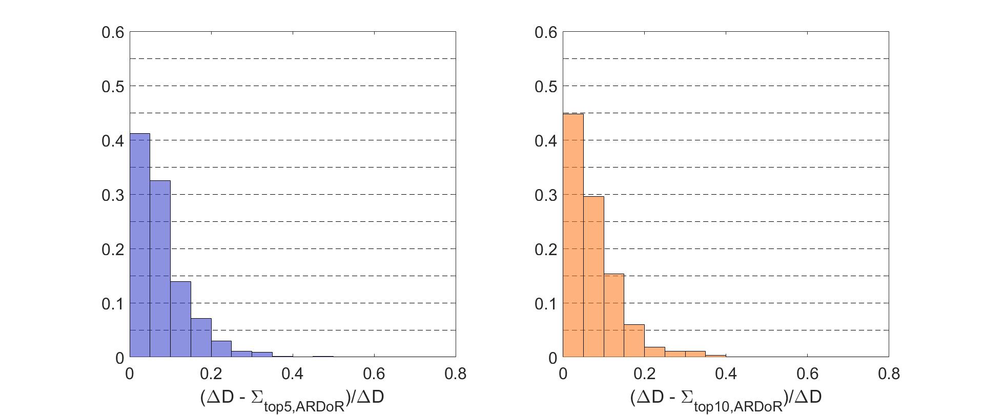
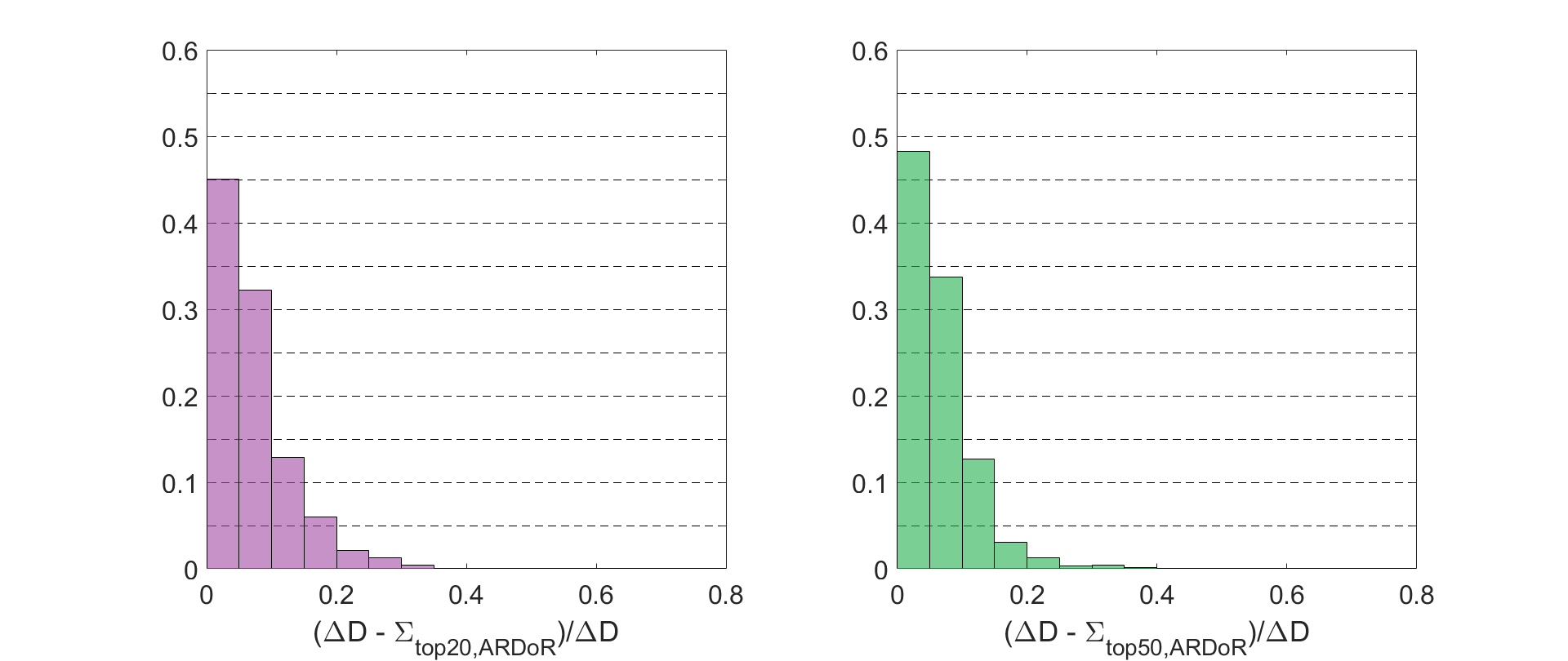
Figure 4: Fractional histograms of the fractional deviation from the absolute change in dipole moment during a solar cycle, calculated summing ultimate AR contributions in the RS case $+$ ARDoR values for ARs with the the top $N$ highest ARDoR. ($N=N_{\mathrm{tot}}$ and $N=0$ for the first and second panels, respectively.) Colour codes are the same as in the previous plots.

4 Conclusions

In Paper 1 we introduced a method to reconstruct variations in the global axial dipole moment of the Sun by an algebraic summation of the contributions from individual active regions. In principle, for the application of this method, for each AR the optimal representation in terms of a simple bipole (or possibly several bipoles in more complex cases) needs to be known. Obtaining this information for thousands of active regions is a nontrivial task, but significant efforts have been made in this direction:

• Wang and Sheeley (1989) determined the properties of bipoles representing close to 3000 ARs with $\Phi>3\cdot 10^{20}\,$Mx from NSO-KP (Kitt Peak) magnetograms in Cycle 21 (1976–1986). Each AR was considered at its maximum development; recurrent ARs were multiply listed.

• Yeates et al. (2007) determined the properties of bipoles representing ARs from NSO-KP/SOLIS synoptic magnetic maps in cycles 23 and 24 (1997–2017). Each AR was considered at central meridian passage; recurrent ARs were multiply listed.

• Whitbread et al. (2018) determined initial dipole moments $D_{1}$ for active regions from Kitt Peak/SOLIS synoptic magnetic maps in cycles 21–24 (1976–2017). Each AR was considered at central meridian passage; recurrent ARs were multiply listed.

• From white-light data without direct magnetic information Jiang et al. (2019) determined an indicative “dipole moment index” for sunspot groups larger than 800 MSH in cycles 21–24 (1976–2017).

Data resulting from the above listed efforts have been placed in public databases. In addition to these, Li and Ulrich (2012) determined tilt angles for 30,600 ARs from Mt.Wilson ad MDI magnetograms in cycles 21–24 (1974–2010). Virtanen et al. (2019b) determined initial dipole moments $D_{1}$ for active regions from Kitt Peak/SOLIS synoptic magnetic maps combined with SDO HMI synoptic maps in cycles 21–24 (1976–2019).

The above studies are limited to the last four cycles when magnetograms were available on a regular basis. For earlier cycles, a number of statistical analyses of sunspot data without direct magnetic information (e.g., Dasi-Espuig et al. 2010, Ivanov 2012, McClintock and Norton 2013, Baranyi 2015, Işık et al. 2018, Senthamizh Pavai et al. 2015) resulted in tilt angle values, offering some potential for use as input for models of the dipole moment evolution. Recently, information on the magnetic polarities of sunspots from Mt.Wilson measurements has been used in combination with Ca II spectroheliograms by Pevtsov et al. (2016) to construct “pseudo-magnetograms” for the period 1915–1985; the results have been benchmarked against direct observations for the last period (Virtanen et al. 2019a).

Despite these impressive efforts, the determination of AR dipole moment values to be used as input in our algebraic method is subject to many uncertainties. As discussed in the Introduction, the available data are increasingly incomplete for smaller ARs. The arbitrariness of the time chosen for the incorporation of ARs is also problematic as during their evolution the structure of ARs can change significantly due to processes not represented in the SFT models (flux emergence or localized photospheric flows). The complexities of AR structure imply that their representation with a single bipole may be subject to doubt (cf. Jiang et al. 2019, Iijima et al. 2019). And for historical data these difficulties are further aggravated.

In view of these considerable difficulties, looking for ways to minimize the need for detailed input data for our algebraic method is advisable. With this objective in mind, in the present work we introduced the ARDoR method and tested it on a large number of activity cycles simulated with the 2$\times$2D dynamo model. We found that

• Including all information on the bipolar active regions appearing in a cycle, our algebraic method can reproduce the dipole moment at the end of the cycle with an error below $\pm 30$ % in over 97 % of cycles.

• Using only positions and magnetic fluxes of the ARs, and arbitrarily equating their polarity separations and tilts to their expected values (reduced stochasticity or RS case), the algebraic method can reproduce the dipole moment at the end of the cycle with an error below $\pm 30$ % in about 74 % of cycles.

• Combining the RS case with detailed information on a small number $N$ of ARs with the largest ARDoR values, the fraction of unexplained cycles is significantly reduced (from 26 % to 12 % in the case of $N=5$ and a $\pm 30$ % accuracy threshold).

These results indicate that stochastic effects on the intercycle variations of solar activity are dominated by the effect of a low number of large “rogue” active regions, rather than the combined effect of numerous small ARs.

Beyond the academic interest of these results, the method has a potential for use in solar cycle prediction. For the realization of this potential, however, a number of further problems need to be addressed. As in forecasts the positions and fluxes of ARs are also not known, the representation of the majority of ARs not faithfully represented in our method must be stochastic also in these variables, or simply replaced by a smooth continuous distribution. Furthermore, for the selection of ARs with the top $N$ ARDoR values these values should be theoretically be computed for all ARs. To avoid this need, “proxies” of ARDoR based on straightforward numerical criteria may need to be identified to select the ARs for which a more in-depth study is then needed to determine ARDoR values. Studies in this direction are left for further research.