Towards an algebraic method of solar cycle prediction

Abstract

We discuss the potential use of an algebraic method to compute the value of the solar axial dipole moment at solar minimum, widely considered to be the most reliable precursor of the activity level in the next solar cycle. The method consists of summing up the ultimate contributions of individual active regions to the solar axial dipole moment at the end of the cycle. A potential limitation of the approach is its dependence on the underlying surface flux transport (SFT) model details. We demonstrate by both analytical and numerical methods that the factor relating the initial and ultimate dipole moment contributions of an active region displays a Gaussian dependence on latitude with parameters that only depend on details of the SFT model through the parameter $\eta/\Delta_{u}$ where $\eta$ is supergranular diffusivity and $\Delta_{u}$ is the divergence of the meridional flow on the equator. In a comparison with cycles simulated in the 2$\times$2D dynamo model we further demonstrate that the inaccuracies associated with the algebraic method are minor and the method may be able to reproduce the dipole moment values in a large majority of cycles.

1 Introduction

Predicting the amplitude of an upcoming solar cycle is the central issue of space climate forecasting. It is widely accepted that the best performing, physically well motivated prediction method is based on the good linear correlation between the solar axial dipole moment in solar activity minimum and the amplitude of the next cycle (Schatten et al. 1978, Wang and Sheeley 2009, Muñoz-Jaramillo et al. 2013, Hathaway and Upton 2016, Petrovay 2020). In order to extend the rather short, 3–4 year long time span of these forecasts, in recent years efforts have been made to “predict the predictor”, i.e. to model and forecast the evolution of the magnetic flux distribution over the solar surface (Jiang et al. 2018).

Starting with the pioneering work of DeVore et al. (1985), the standard approach to this problem has been the use of surface flux transport (SFT) simulations. This approach assumes that the line-of-sight magnetic field component shown in synoptic maps constructed from solar magnetograms corresponds to the projection of an inherently radial mean photospheric magnetic field with strength $B_{r}$, the transport of which is governed by advection due to large scale flows and diffusion due to supergranular motions:

$$\frac{\partial B_{r}}{\partial t} = \displaystyle-\Omega(\lambda)\,\frac{\partial B_{r}}{\partial\phi}-\frac{1}{R\cos{\lambda}}\,\frac{\partial}{\partial\lambda}\left[B_{r}\,u(\lambda)\cos{\lambda}\right]$$ (1)

$$+\frac{\eta}{R^{2}}\left[\frac{1}{\cos\lambda}\,\frac{\partial}{\partial\lambda}\left(\cos{\lambda}\,\frac{\partial B_{r}}{\partial\lambda}\right)+\frac{1}{\cos^{2}\lambda}\,\frac{\partial^{2}B_{r}}{\partial{\phi}^{2}}\right]-\frac{B_{r}}{\tau}+S_{r}(\lambda,\phi,t),$$

where $t$ is time, $\lambda$ and $\phi$ are heliographic latitude and longitude, $R$ is the radius of the Sun, $\Omega$ is the angular velocity of differential rotation, $u(\lambda)=u_{0}f(\lambda)$ is the meridional flow, and $\eta$ is the supergranular diffusivity. The source term $S_{r}$ represents the emergence of new flux into the atmosphere in active regions, while the term $-B_{r}/\tau$ is the simplest (though not the most realistic) form of a sink term representing the effects of radial diffusion that would appear in a consistent derivation of the transport equation from the radial component of the induction equation. (For further discussion of the decay term see e.g. Baumann et al. 2006, Whitbread et al. 2017 or Petrovay and Talafha 2019. For general reviews of the SFT modelling approach see Sheeley 2005, Mackay and Yeates 2012, Jiang et al. 2014b, Wang 2017).

Numerous studies have been performed with the objective to reproduce and predict the evolution of the solar dipole moment (Wang and Sheeley 1991, Whitbread et al. 2017, Virtanen et al. 2017). Despite some spectacular successes, this approach still suffers from two main limitations:

(1) Ill constrained SFT model ingredients. The model has at least 3 free numerical parameters ($u_{0}$, $\eta$, $\tau$) as well as a free function, the observationally not well mapped meridional flow profile $f(\lambda)$. Attempts to determine the ingredients from direct observations have dubious relevance and often yield contradictory results. Internal optimizations of the model, in turn, result in parameter combinations that may depend on the choice of merit and still allow a rather wide freedom in the choices (Lemerle et al. 2015, Virtanen et al. 2017, Whitbread et al. 2017, Petrovay and Talafha 2019). The ill constrained ingredients imply that in order to obtain a realistic estimate of the uncertainities in the predictions an ensemble of models with varying parameters should be studied; with the need to numerically solve the partial differential equation (1) for each of these models the process can get rather lengthy and cumbersome.

(2) A realistic representation of the active region source. These sources are often represented as simple bipoles instantaneously introduced into the simulation, or, more realistically, by assimilating actual magnetograms taken at the time of their central meridian passage. In reality, however, during the evolution of an active region its magnetic flux distribution keeps changing as a consequence of the emergence of new flux and the proper motions of sunspots and other magnetic flux concentrations driven by subsurface dynamics and/or by random, localized photospheric flows —effects which are not accounted for in the SFT model. The choice of the proper form of the source and the time of its introduction is therefore a highly nontrivial problem. And the very large number (thousands) of active regions arising in a solar cycle makes this task challenging even in the simplest, idealized case of bipole representation. These problems are even further aggravated in the case of historical data, when the objective is to understand and reproduce the course of evolution of solar activity in centuries past.

The objective of this paper is to consider ways to alleviate these difficulties by simplifying the prediction method to its bare essentials. Specifically, in Section 2 we will show that the SFT modelling approach of solving a partial differential equation can be reduced to the calculation of an algebraic sum. Sections 3 and 4 demonstrate that the result of this procedure only depends on two numerical combinations of the model parameters without the need to specify the choice of any unknown function. Then, in Section 5 we validate the approach in a comparison with activity cycles simulated in a dynamo model. These results may pave the way towards a more robust and effective approach to solar cycle prediction.

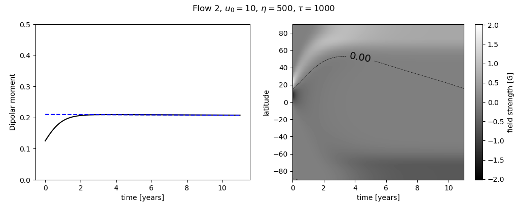
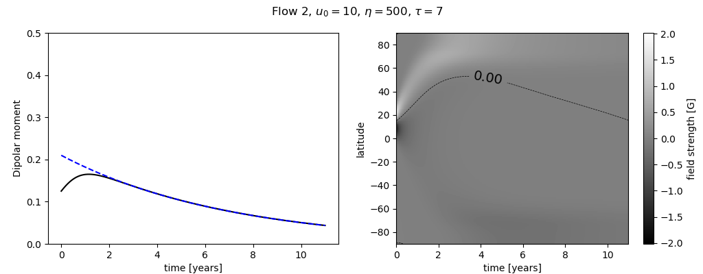
Figure 1: Solutions of the 1D SFT equation with a bipolar source placed at $\lambda_{0}=+15^{\circ}$ latitude at time $t=0$. Units of the model parameters shown on top of the rows are m$/$s, km${}^{2}/$s and year, respectively. The meridional flow profile is given by eq. (9). Dashed blue lines in the left-hand plots mark the asymptotic solutions $D=\delta D_{\infty}$ (top) and $D=\delta D_{\infty}\exp(-t/\tau)$ (bottom).

2 Mathematical formulation of the problem

The axial dipolar moment of the Sun is given by

$$D(t)=\frac{3}{2}\int_{-\pi/2}^{\pi/2}B(\lambda,t)\sin\lambda\cos\lambda\,\mathrm{d}\lambda,$$ (2)

where $B=\frac{1}{2\pi}\int_{0}^{2\pi}B_{r}\,d\phi$ is the azimuthally averaged field strength. Throughout this paper, $D$ will denote the global dipole moment of the whole Sun as defined in equation (2), while $\delta D$ will denote the contribution to $D$ from an individual active region. The evolution of $B$, and consequently $D$, is determined by the 1D surface flux transport equation obtained by azimuthally integrating equation (1):

$$\frac{\partial B}{\partial t}=\displaystyle-\frac{1}{R\cos{\lambda}}\,\frac{\partial}{\partial\lambda}\left[B\,u(\lambda)\cos{\lambda}\right]+\frac{\eta}{R^{2}}\frac{1}{\cos\lambda}\,\frac{\partial}{\partial\lambda}\left(\cos{\lambda}\,\frac{\partial B}{\partial\lambda}\right)-\frac{B}{\tau}+S(\lambda,t),$$ (3)

where $S=\frac{1}{2\pi}\int_{0}^{2\pi}S_{r}\,d\phi$.

In this azimuthally averaged representation a tilted bipolar region is then a pair of flux rings of opposite polarity, appearing as a bipole source with a finite latitudinal separation in equation (3)

Figure 1 presents solutions of equation (3) for a particular case where the source is a single bipole placed at $\lambda_{0}=+15^{\circ}$ latitude at time $t=0$. Both polarities were assumed to initially have a Gaussian profile in $\lambda$ with a half-width $\sigma_{0}=6^{\circ}$. The left-hand panels show the evolution of the axial dipolar moment. The right-hand panels display the evolution of $B$ in the time-latitude plane. The cases shown in the top and bottom rows only differ in the value of $\tau$: in the first case $\tau$ is effectively infinite (no decay), while in the second case it is shorter than the solar cycle period. As it is easy to understand from the structure of eq. (3), the two solutions only differ by the presence of an exponential factor $\exp(-t/\tau)$ when $\tau$ is finite.

The evolution is determined by the competition of two processes. The diffusive spreading of the two polarity patches of opposite sign leads to the cancellation of a large part of the flux originally present, yet a small fraction of the flux still manages to reach the Southern hemisphere where it is transported to the South pole by the meridional flow. The “leading” polarity flux patch, situated closer to the equator, gives a larger contribution to the flux ultimately reaching the South pole, so in the final state, a leading polarity patch remains at the South pole, while a corresponding trailing polarity patch remains at the North pole. While the flux in these patches is a fraction of the original flux in the region, their high latitudinal separation gives rise to a dipole moment that, in the case plotted in Fig. 1, exceeds the initial value. In the limit $\tau\rightarrow\infty$ the dipole moment remains very nearly constant at a fixed value $\delta D_{\infty}(\lambda_{0})$. For finite $\tau$ the dipole moment asymptotically behaves as $\delta D_{\infty}\exp(-t/\tau)$.

This implies that if, ignoring the complex details of its structure and evolution, the $i$th active region in cycle $n$ (starting at time $t_{n}$) is represented by a simple dipole instantaneously introduced into the SFT model at time $t_{i}$ with an initial dipole moment $\delta D_{1,i}$, the ultimate contribution of all active regions at the end of the cycle will be given by

$$\Delta D_{n}\equiv D_{n+1}-D_{n}=\sum_{i=1}^{N_{\mathrm{tot}}}\delta D_{U,i}=\sum_{i=1}^{N_{\mathrm{tot}}}\delta D_{\infty,i}\,e^{(t_{i}-t_{n+1})/\tau}=\sum_{i=1}^{N_{\mathrm{tot}}}{f_{\infty,i}}\,\delta D_{1,i}\,e^{(t_{i}-t_{n+1})/\tau},$$ (4)

where $N_{\mathrm{tot}}$ is the total number of ARs in the cycle, $\delta D_{U}$ is the ultimate contribution of an active region to the global dipole moment at the end of a cycle, and the asymptotic dipole contribution factor is

$$f_{\infty}=\delta D_{\infty}/\delta D_{1}.$$ (5)

From equation (2) it is straightforward to show that for a pointlike bipole consisting of a pair of pointlike polarities with a small latitudinal separation $d_{\lambda}$ the initial dipole moment contribution $\delta D_{1}$ is given by

$$\delta D_{1}=\frac{3}{4\pi R^{2}}\,\Phi\,d_{\lambda}\cos\lambda_{0},$$ (6)

where $\Phi$ is the magnetic flux in the northern flux patch.

Equations (4)–(6) offer a simple algebraic tool to extend the temporal scope of the polar field precursor method by “predicting the precursor”, i.e. computing the dipole moment built up during a solar activity cycle without the need to solve the partial differential equation (3) or (1). For the case of cycle 23 this approach has been already exploited by Jiang et al. (2019) for one particular SFT model setup.

Generally, however, this approach is subject to a number of limitations. These limitations were already outlined in the Introduction above. In more detail, they are:

(1a) The result depends on details of the SFT model used, mainly through the $f_{\infty,i}$, and for models with a decay term also through the exponential factor in (4).

(1b) As illustrated in Fig. 1, the asymptotic solution is approximated after a transitional period of 2–3 years only. The contribution of active regions emerging in the last years of the cycle is therefore not accurately represented by this formula. As, however, activity in this late phase of the cycle is normally rather low, this is not expected to be a major limitation in most cases.

(2a) The assumption that active regions may be represented by the instantaneous introduction of simple bipoles into the simulation is undoubtedly a strong simplification.

(2b) The number $N_{\mathrm{tot}}$ of terms in the sum, i.e. the number of bipolar regions contributing to the solar axial dipole moment can be quite high.

In the present work we focus on issues (1a), (1b) and (2a). Issue (2b) will be dealt with in a companion paper.

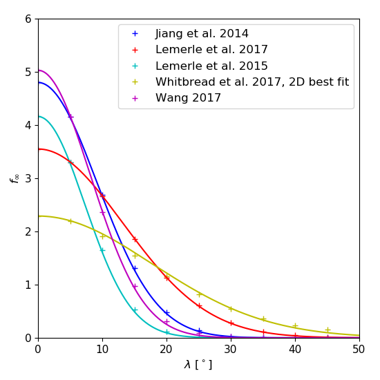
Figure 2: Dependence of the asymptotic dipole contribution factor $f_{\infty}$ of bipolar sources on their latitude in various SFT model setups. Solid lines are Gaussian fits to the numerical results.

3 Calculating the ultimate dipole contribution of active regions

The dependence of the asymptotic dipole contribution factor $f_{\infty}$ on latitude was first considered by Jiang et al. (2014a). In a series of numerical experiments with one particular SFT model they found a Gaussian dependence on latitude:

$$f_{\infty}=A\exp(-\lambda_{0}^{2}/2\lambda_{R}^{2}).$$ (7)

In what follows, $\lambda_{R}$ will be referred to as the dynamo effectivity range of active regions.

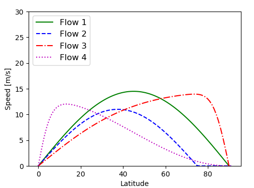
Figure 3: The meridional flow profiles used in the paper.

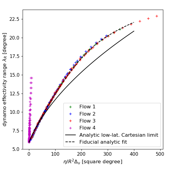
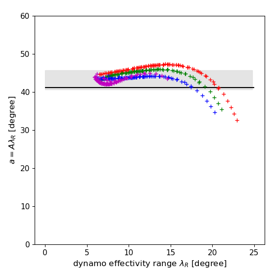
Figure 4: Dependence of the dynamo effectivity range $\lambda_{R}$ (left) and the amplitude $A$ (right) of the asymptotic dipole contribution factor of bipolar sources on selected parameter combinations in various SFT model setups for $\sigma_{0}=6^{\circ}$. In the left-hand panel the solid line shows the analytic result (22) in the low-latitude Cartesian limit, while the dashed line shows a fiducial analytic fit of the type (26). In the right-hand panel the shaded region is the range expected for a $\sin^{n}\lambda$ equilibrium polar field profile with $n>7$; the horizontal line marks the value for $n=8$.

Let us consider whether this conclusion holds generally for other SFT model setups. In Fig. 2 the results of a similar set of experiments for different model setups are shown: in addition to Jiang et al.’s original setup, the other SFT models used were those of Lemerle et al. (2015) , Lemerle and Charbonneau (2017), Whitbread et al. (2017) and Wang (2017). It is apparent that the Gaussian dependence identified by Jiang et al. (2014a) holds generally. Indeed, even in an SFT model where active region shapes are determined by assimilation rather than fitted with bipoles, Whitbread et al. (2018) still found a Gaussian. In all these cases, however, the width and amplitude of the Gaussian are different. It was indeed already found by Nagy et al. (2017) that the dynamo effectivity range in the case of the Lemerle and Charbonneau (2017) setup was significantly wider than expected from the results of Jiang et al. (2014a).

In order to understand the dependence of $\lambda_{R}$ and $A$ on model parameters we determine these parameters on a large grid of SFT models. Our model grid is essentially identical to the grid considered by Petrovay and Talafha (2019), except that here we limit ourselves to models with effectively no decay term ($\tau=1000\,$years) as the effect of $\tau$ has already been separated in the exponential factor in eq. 4. Four types of flow profiles are considered (cf. Fig. 3).

Flow 1: a simple sinusoidal profile

$$u=u_{0}\sin(2\lambda)$$ (8)

Flow 2: a sinusoidal profile with a dead zone around the poles,

$$u=\left\{\begin{array}[]{ll}u_{0}\sin(\pi\lambda/\lambda_{0})&\mbox{if }|\lambda|<\lambda_{0}\\ 0&\mbox{otherwise }\end{array}\right.$$ (9)

Flow 3: The Lemerle and Charbonneau (2017) profile peaking at high latitudes,

$$u=\frac{u_{0}}{u_{0}^{\ast}}\mbox{erf}\,(V\cos{\lambda})\,\mbox{erf}\,(\sin{\lambda})\qquad u_{0}^{\ast}=0.82\qquad V=7$$ (10)

Flow 4: A profile peaking at very low latitudes, considered by Wang (2017):

$$u=1.08\,u_{0}\,\tanh(\lambda/6^{\circ})\,\cos^{2}\lambda$$ (11)

For each of the profiles, $u_{0}$ was allowed to vary between 5 and 20 m/s in steps of 2.5, while $\eta$ varied from 50 to 750 km${}^{2}/$s in steps of 50. From numerical runs like the one plotted in Fig. 1 the values of $\lambda_{R}$ and $A$ were determined for each model.

Experimenting with different simple combinations of the input and output parameters we find the clearest relationship in the case plotted in Fig. 4. Here,

$$\Delta_{u}=\frac{1}{R}\left.\frac{{\mathrm{d}}u}{{\mathrm{d}}\lambda}\right|_{\lambda=0}$$ (12)

is the divergence of the meridional flow at the equator.

The finding that the single parameter combination $\eta/\Delta_{u}$ determines $f_{\infty}$ for all but one of our 2-parameter model grids, irrespective of the choice of the meridional flow profile is an impressive and somewhat unexpected result which calls for a theoretical interpretation.

4 Analytical derivation of the asymptotic dipole contribution factor

4.1 Low-latitude Cartesian limit

To make the problem analytically tractable, we limit ourselves to the neighbourhood of the equator ($\lambda\ll 1$ radian) where the spherical coordinate grid may be locally approximated by a Cartesian setup and meridional flow is expressed by the leading term of its Taylor expansion as $u=R\Delta_{u}\lambda$ with $\Delta_{u}=$const. This is formally identical to the cosmological case of a one-dimensional Hubble flow in a vacuum dominated universe and the advection of a frozen-in magnetic field configuration by the flow is an exponential expansion. This cosmological analogy suggests to consider the evolution in the Lagrangian comoving (co-expanding) frame, where fluid elements are labelled by their latitude $\lambda_{L}$ at time zero, rather than their current latitude $\lambda=\mathrm{e}^{\Delta_{u}t}\lambda_{L}$.

We recall the initial condition of the evolution, as illustrated in Fig. 1: a pair of opposite polarity flux rings with Gaussian profile of half width $\sigma_{0}\ll 1$ radian, situated at latitude $\lambda_{0}$, with a separation $d_{\lambda}\ll 1$ radian between the rings. (In the diffusive case, other assumed initial profiles will also soon approach Gaussian by virtue of the central limit theorem.) What we are looking for is the amount of net transequatorial flux (flux in the other hemisphere) in the limit $t\rightarrow\infty$.

4.1.1 Asymptotic magnetic field profile

In the Lagrangian frame flow advection is absent by definition, so the flux transport equation simplifies to a diffusion equation

$$\frac{dB_{L}}{dt}=\frac{\eta_{L}}{R^{2}}\frac{\partial^{2}B_{L}}{\partial{\lambda_{L}}^{2}},$$ (13)

where, however, the diffusivity $\eta_{L}(t)$ is now time dependent. Indeed, in the comoving frame the unit of length expands exponentially as $\exp(\Delta_{u}t)$, so the diffusivity, of dimension length${}^{2}/$time, expressed in these units, will scale as $\eta_{L}\propto e^{-2\Delta_{u}t}$. For the same reason, the Lagrangian flux density $B_{L}$ is related to the Eulerian by $B=B_{L}\mathrm{e}^{-\Delta_{u}t}$.

Consider the evolution of one of the two flux patches comprising the bipole. Our initial condition is

$$B_{L}(\lambda_{L},0)=\frac{a}{\sigma_{0}}\exp-\frac{(\lambda_{L}-\lambda_{0})^{2}}{2\sigma_{0}^{2}}.$$ (14)

This problem may be solved exactly using Fourier transforms (cf. Mackay et al., 2016). First, we change the time variable from $t$ to $t^{\prime}={\textstyle\frac{1}{R^{2}}}\int_{0}^{t}\eta_{L}(\tilde{t})\,\mathrm{d}\tilde{t}$ to obtain the standard diffusion equation

$$\frac{\partial B_{L}}{\partial t^{\prime}}=\frac{\partial^{2}B_{L}}{\partial\lambda_{L}^{2}},$$ (15)

which may be solved using standard techniques. In particular, if we define the Fourier transform

$$\hat{B}_{L}(k,t^{\prime})=\frac{1}{2\pi}\int_{-\infty}^{\infty}B_{L}(\lambda_{L},t^{\prime})\mathrm{e}^{-ik\lambda_{L}}\,\mathrm{d}\lambda_{L}$$ (16)

then equation (15) implies that $\hat{B}_{L}(k,t^{\prime})=\hat{B}_{L}(k,0)\mathrm{e}^{-k^{2}t^{\prime}}$. The Fourier transform of our initial condition is

$$\hat{B}_{L}(k,0)=\frac{a}{\sqrt{2\pi}}\exp-\frac{\sigma_{0}^{2}k^{2}+2\lambda_{0}ki}{2}.$$ (17)

Inverting the transform finally gives

$$B_{L}(\lambda_{L},t^{\prime})=\int_{-\infty}^{\infty}\hat{B}_{L}(k,t^{\prime})\mathrm{e}^{ik\lambda_{L}}\,\mathrm{d}k=\frac{a}{\sqrt{2t^{\prime}+\sigma_{0}^{2}}}\exp-\frac{(\lambda_{L}-\lambda_{0})^{2}}{2(2t^{\prime}+\sigma_{0}^{2})}.$$ (18)

Since $t^{\prime}=-\frac{\eta}{2R^{2}\Delta_{u}}(\mathrm{e}^{-2\Delta_{u}t}-1)$, we arrive at

$$B_{L}=\frac{a}{\sigma(t)}\exp-\frac{(\lambda_{L}-\lambda_{0})^{2}}{2\sigma(t)^{2}},$$ (19)

with

$$\sigma(t)=\left[\sigma_{0}^{2}+\frac{\eta}{R^{2}\Delta_{u}}(1-e^{-2\Delta_{u}t})\right]^{1/2}.$$ (20)

Note that this self-similar solution might have been anticipated, given that the Gaussian is known to be a self-similar solution of the diffusion equation and the meaning of $B_{L}$ is [one-dimensional] flux density, so magnetic flux conservation requires the amplitude of the Gaussian to scale with the inverse of $\sigma$. Plugging eq. (19) back into (13) then returns (20).

4.1.2 Transequatorial flux

In the $t\rightarrow\infty$ limit equation (19) gives

$$B_{L,\infty}=\frac{a}{\lambda_{R}(t)}\exp-\frac{(\lambda_{L}-\lambda_{0})^{2}}{2\lambda_{R}(t)^{2}},$$ (21)

with

$$\lambda_{R}=\lambda_{R,\mathrm{limit}}\equiv\left(\sigma_{0}^{2}+\frac{\eta}{R^{2}\Delta_{u}}\right)^{1/2}.$$ (22)

Using equation (21), and taking $\lambda_{0}>0$ for concreteness, the fraction of flux of this single polarity in the opposite (Southern) hemisphere is given by

$$f_{\Phi}(\lambda_{0})=\int_{-\infty}^{0}B_{L,\infty}\,d\lambda_{L}\left/\int_{-\infty}^{\infty}B_{L,\infty}\,d\lambda_{L}\right.=\frac{1}{2}\left[1-{\rm erf}\,(\lambda_{0}/\sqrt{2}\lambda_{R})\right].$$ (23)

For our pair of flux rings separated by $d_{\lambda}$, the net transequatorial flux fraction is then

$$\Phi_{\infty}/\Phi_{1}=f_{\Phi}(\lambda_{0}-d_{\lambda}/2)-f_{\Phi}(\lambda_{0}+d_{\lambda}/2)\simeq\frac{d_{\lambda}}{2^{1/2}\pi^{1/2}\lambda_{R}}\exp{\frac{-\lambda_{0}^{2}}{2\lambda_{R}^{2}}},$$ (24)

where the last form is the leading term in a Taylor expansion for small $d_{\lambda}$.

4.2 Sphericity effects

To compute the asymptotic dipole contribution $\delta D_{\infty}$ from $\Phi_{\infty}$ by equation (2) we need to return to spherical geometry. The poleward meridional flow results in a “topknot” equilibrium field distribution strongly peaked near the poles (Sheeley et al. 1989). Indeed, approximating the field profile as $B(\lambda)\propto\sin^{n}\lambda$, even flows mildly concentrated on the poles will result in $n\simeq 7$ (cf. Fig. 4 in Wang 2017). Observational constraints indicate $n\ga 8$–$9$ (Petrie 2015). With this approximation, using eqs. (2), (5), (6) and (24), we have the following expression for the asymptotic dipole contribution factor in the low-latitude limit:

$$f_{\infty}=\frac{a}{\lambda_{R}}\exp{-\frac{\lambda_{0}^{2}}{2\lambda_{R}^{2}}}\qquad\mathrm{with}\qquad a=\left(\frac{2}{\pi}\right)^{1/2}\frac{n+1}{n+2}.$$ (25)

(A factor $1/\cos\lambda_{0}$ originating from (6) has been omitted as in the low-latitude limit it becomes unity.) For $n=8$ this yields $a=41{\hbox{$.\!\!^{\circ}$}}16$; values for $n>7$ are in the range between $40{\hbox{$.\!\!^{\circ}$}}66$ and $45{\hbox{$.\!\!^{\circ}$}}7$. The curves in the right-hand panel of Figure 4 are in agreement with this result.

The curves representing flow types 1 to 3 in the left-hand panel of Fig. 4 are well fitted by the solution (22) at low values of $\lambda_{R}$. This is to be expected as these flows peak at latitudes above $40^{\circ}$ so for low latitudes the profiles are well approximated as linear. For the same reason, while for values $\lambda_{R}\sim 10$–$20^{\circ}$ curvature effects do come into play, the curves still do not diverge as the nonlinearity of the flow profile remains low, hence, with an appropriate planar projection of the spherical surface, the flow may still be transformed out switching to a homologously expanding Lagrangian frame. In this case equation (13) generalizes to the diffusion equation on a spherical surface which has no flux-conserving solution with an exactly Gaussian profile, though Figure 2 indicates that at moderate latitudes the solutions may still be well approximated by a Gaussian. The dynamo effectivity range, however, changes. A good empirical fit to the curves is found to be

$$\lambda_{R,\mathrm{fit}}=g^{1/2}(x=\eta/R^{2}\Delta_{u})\lambda_{R,\mathrm{limit}}$$ (26)

with

$$g(x)=(m_{1}x+c_{1})\{1-\tanh[(x-c_{0})/w]\}+(m_{2}x+c_{2})\tanh[(x-c_{0})/w].$$ (27)

The points representing flow type 4 in the left-hand panel of Fig. 4 strongly diverge from both equation (22) and (26). The reason is that for this profile peaking at very low latitude, the nonlinearity of the profile becomes important already at $\lambda\sim\sigma_{0}$. In effect, in most of the area covered by the AR flux during its evolution the expansion rate will be far below the nominal equatorial value —at $\lambda>13^{\circ}$ the surface will actually already contract, strengthening the field. Hence, nominal values of the parameter $\eta/\Delta_{u}$ are not really relevant for the determination of $\lambda_{R}$ in this case.

To close off our analytic discussion we note that the expression (22) for the dynamo effectivity range can also be understood in simple physical terms. The time scale associated with diffusion to the other hemisphere from latitude $\lambda$ is $(R\lambda)^{2}/\eta$. The latitude where this equals the advective time scale $1/\Delta_{u}$ is just $(\eta/{R^{2}\Delta_{u}})^{1/2}$: for higher latitudes diffusion cannot compete with the poleward advection and little flux from here can reach the other hemisphere.

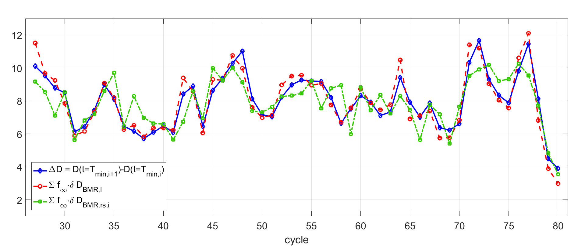
Figure 5: Comparison of total net change in the solar axial dipole moment $|D_{n+1}-D_{n}|$ in the 2$\times$2D dynamo simulation and its approximations with the algebraic method in a segment of 80 cycles. Plotted are absolute values of the quantities shown in the legend. See text for further explanations.

5 Comparison to a dynamo model solution

Our suggested algebraic approach to solar cycle prediction consists in using equation (4) to calculate the net dipole moment at the end of a solar cycle, where the dynamo effectivity $f_{\infty}$ is given by eq. (25), with $\lambda_{R}$ and $a$ taken from either a direct interpolation of the numerical results plotted in Fig. 4, from their analytical approximation (dashed curve) or even from the low-latitude limit (22).

In order to test the validity and accuracy of the suggested algebraic approach, in Fig. 5 we compare the results of a run of the 2$\times$2D dynamo model, as described in Lemerle and Charbonneau (2017), with the results of our algebraic approach. For the SFT parameters used in the Lemerle and Charbonneau (2017) model ($u_{0}^{\ast}=0.82$, $u_{0}=17\,$m$/$s, $\eta=600\,$km${}^{2}/$s, $\tau=10\,$yr) the numerical results plotted in Fig. 4 give $\lambda_{R}=13{\hbox{$.\!\!^{\circ}$}}6$ and $A=3.75$. The advantage of using the 2$\times$2D model is that it explicitly includes a 2D SFT model as one of its components, with the source term represented as idealized bipoles with parameters that can be directly extracted from the models. In this way, factors like an arbitrary choice of model parameters or ill-specified sources will not influence the comparison.

Plotted in blue is the net change in the axial dipole moment $|D_{n+1}-D_{n}|$ between subsequent minima of the cycle in the model. The red dashed curve shows the values computed by adding to the actual dipole moment at the start of a cycle the expected total dipole moment contribution calculated by the algebraic method, eqs. (4) and (25), with the parameter values quoted above; $\delta D_{1,i}$ values are computed using the BMR properties extracted from the dynamo code. While the overall agreement is quite good, some smaller discrepancies remain. The standard deviation of the relative error is 10.1 %. Sources contributing to this unexplained variance include the invalidity of formula (4) for active regions emerging in the last three years of each cycle: as illustrated in Fig. 1, in these cases the time elapsed from emergence to solar minimum is too short for the asymptotic solution to set in. Other contributing factors are smaller differences in model details between the 2$\times$2D model and the 1D SFT model forming the basis of our algebraic approach.

The green dashed curve, in turn, diplays the result of the algebraic method for the “reduced stochasticity” case. In this case, bipolar magnetic regions (as the active regions are called in the 2$\times$2D model) are substituted with regions of the same flux and latitude, but with tilt and polarity separation values corresponding to the expected values for the given flux and latitude, as given by eqs. (15) and (16a) in Lemerle et al. (2015). While the agreement is noticeably poorer (standard deviation of the relative error now reaches 21.2 %), the net dipole moment change is still reproduced with less than 25% error in about 90 % of the cases. This indicates that detailed knowledge of the structure and evolution of each individual active region may not be indispensable for a tolerably good predictive skill in the algebraic method in most (though not all) cycles. This issue will be discussed further in the second paper of this series (Nagy et al. 2020).

6 Conclusions

We have discussed the potential use of an algebraic method to predict the value of the solar axial dipole moment at solar minimum. The method, already applied in the case of one particular SFT model by Jiang et al. (2019), consists in summing up the ultimate contributions of individual active regions the solar axial dipole moment as given by equations (4) and (25).

In Section 2 we listed four potential limitations of the approach. The first of these, (1a) was its dependence on SFT model details. Indeed, the meridional flow profile is still rather uncertain and potentially variable; in addition, systematic inflows towards the activity belts are also expected to impact on flux transport, see Nagy, Lemerle and Charbonneau (2020, in this issue). Disregarding time dependent effects here we demonstrated by both analytical and numerical methods that the dynamo effectivity range $\lambda_{R}$ and the equatorial value of the asymptotic dipole contribution factor $A$ only depend on details of the SFT model through the parameter $\eta/\Delta_{u}$. This significantly reduces the uncertainty introduced by the choice of model details and makes the algebraic method preferable to the more computation-intensive traditional method of numerically solving the SFT equation.

While numerical costs and a more limited freedom in the choice of parameters advocate the use of this algebraic approach, this clearly goes at the cost of accuracy. One source of the inaccuracy, (1b), is inapplicability of the ultimate dipole contribution to active regions appearing in the last years of a solar cycle, as the contributions of such ARs have not yet reached equilibrium at the time of minimum. In a comparison with cycles simulated in the 2$\times$D dynamo model we demonstrated that the inaccuracy introduced by this effect and by differences in the underlying numerical models is small and does not constitute a great obstacle in the way of correctly reproducing the dipole moment.

Another source of inaccuracy of this approach, (2a), is that the representation of active region sources by idealized bipoles is likely to be far from perfect. Applying our method to the same dynamo-simulated cycles but substituting the assumed initial AR dipole moments with their expected values for an AR of the given size and latitude showed that in this case the dipole moment could still be reasonably well reproduced in the large majority of cycles, lending further support to the algebraic approach. Nevertheless, in a small fraction of cycles inaccurate representation of the sources does lead to significant inaccuracies in the resulting dipole moment values. Note that while in the dynamo model used here for comparison ARs were assumed to be be bipolar, in applications to solar data a further source of uncertainty concerns to what extent a bipolar representation reflects the structure of ARs (cf. Iijima et al. 2019, Jiang et al. 2019, Yeates 2020).

The fourth limitation of the method, (2b) is related to the very high number of terms in the summation that are theoretically needed for the correct representation of the dipole contributions, which exacerbates the issue with the correct representation of the initial AR contributions. On the other hand, the fact that there are many regions might help fluctuations from the Gaussian trend to average out in an overall prediction. This issue will be discussed further in the second part of this series.