∎
22email: jiejiang@nao.cas.cn 33institutetext: D. H. Hathaway 44institutetext: NASA/MSFC, Huntsville, AL 35812, USA
44email: david.hathaway@nasa.gov 55institutetext: R. H. Cameron 66institutetext: Max-Planck-Institut für Sonnensystemforschung, Justus-von-Liebig-Weg 3, 37077 Göttingen, Germany
66email: cameron@mps.mpg.de 77institutetext: S. K. Solanki 88institutetext: Max-Planck-Institut für Sonnensystemforschung, Justus-von-Liebig-Weg 3, 37077 Göttingen, Germany
and School of Space Research, Kyung Hee University,Yongin, Gyeonggi-Do,446-701, Korea
88email: solanki@mps.mpg.de 99institutetext: L. Gizon 1010institutetext: Max-Planck-Institut für Sonnensystemforschung, Justus-von-Liebig-Weg 3, 37077 Göttingen, Germany
and Georg-August-Universität Göttingen, Institut für Astrophysik, Friedrich-Hund-Platz 1, 37077 Göttingen, Germany
1010email: gizon@mps.mpg.de 1111institutetext: L. Upton 1212institutetext: Vanderbilt University, Nashville, TN 37235 USA 1313institutetext: The University of Alabama in Huntsville, Huntsville, Al 35899 USA
1313email: lar0009@uah.edu
Magnetic Flux Transport at the Solar Surface
Abstract
After emerging to the solar surface, the Sun’s magnetic field displays a complex and intricate evolution. The evolution of the surface field is important for several reasons. One is that the surface field, and its dynamics, sets the boundary condition for the coronal and heliospheric magnetic fields. Another is that the surface evolution gives us insight into the dynamo process. In particular, it plays an essential role in the Babcock-Leighton model of the solar dynamo. Describing this evolution is the aim of the surface flux transport model. The model starts from the emergence of magnetic bipoles. Thereafter, the model is based on the induction equation and the fact that after emergence the magnetic field is observed to evolve as if it were purely radial. The induction equation then describes how the surface flows – differential rotation, meridional circulation, granular, supergranular flows, and active region inflows – determine the evolution of the field (now taken to be purely radial). In this paper, we review the modeling of the various processes that determine the evolution of the surface field. We restrict our attention to their role in the surface flux transport model. We also discuss the success of the model and some of the results that have been obtained using this model.
1 Introduction
The magnetic fields on the Sun are generated by dynamo action, ultimately driven by convective motions beneath the Sun’s surface (Charbonneau, 2010). Many of the physically important dynamo processes take place beneath the solar surface, where the details are mostly hidden from us. The tools we have for probing the subsurface dynamics of the magnetic fields are theory and helioseismology, both of which have unveiled some of the dynamics (for a review of helioseismic results see Gizon and Birch, 2005).
Our knowledge of the magnetic field dynamics at the solar surface can be inferred from high resolution spectropolarimetric observations, for example, the Hinode spacecraft with about 230 km resolution (Tsuneta et al., 2008) and the Sunrise balloon-borne solar observatory with about 100 km resolution (Solanki et al., 2010), and is consequently much richer in detail. The magnetic field at the solar surface is observed to be structured on all spatial scales we can observe - from below the resolution limit of the largest available solar telescopes to the scale of the whole Sun (Solanki et al., 2006). In this review, we will concentrate exclusively on the evolution of the large-scale magnetic fields at the solar surface.
One reason for studying the evolution of the large-scale magnetic field on the solar surface is because that it sets the structure of the heliospheric magnetic field (Mackay and Yeates, 2012). A second reason is that it is the observable part of the solar dynamo. In the context of the Babcock-Leighton dynamo (Babcock, 1961; Leighton, 1964), the surface evolution is particularly important because the source of poloidal flux in this model is the emergence and subsequent evolution of tilted magnetic bipolar regions.
The evolution of the surface magnetic field is, in its simplest form, almost trivial. Magnetic flux emerges at the solar surface in the form of bipolar magnetic regions. The flux is then transported and dispersed over the solar surface due to systematic and turbulent motions. Lastly, when magnetic flux of opposite polarity come into contact, the features cancel, removing equal amounts of flux of each sign.
These processes are modeled by the surface flux transport equation, which describes the evolution of the radial component of the magnetic field on the solar surface. The equation is the -component of the MHD induction equation at under the assumption that the field at the surface is purely vertical, augmented by a source term for , and flux removal term, and respectively (see DeVore et al., 1984) . The equation for the radial component of the field at is then
| (2) |
where is the velocity in the longitudinal () direction, is the velocity in the latitudinal () direction, is the horizontal diffusivity at the surface (which we have assumed is uniform), is some operator representing the removal of flux from the surface, and is a source term describing the emergence of new flux rising from below, and are the solar longitude and colatitude respectively and is the solar radius.
In principle, both the the surface velocity, , and the radial component of the magnetic field are structured on all scales from tens of meters to the size of Sun, and evolves on time scales of seconds for the small scales to years for the largest scales. This renders the full problem intractable. For almost all problems, however, the full range of scales do not need to be dealt with, and average values of and can be used, with smaller unresolved velocities being treated as an enhanced diffusivity . There is no single best choice of what temporal or spatial averaging should be done: different temporal and spatial averaging allow different science questions to be addressed.
In the following sections we will add flesh to Eq. (1) by describing in detail the relevant physical processes and the ways in which they can be modeled. We start with a deeper exposition of the basis for the surface flux transport model in Section 2. Then we describe some of the ways in which the source term can be constructed in Section 3, and the flows and diffusivity in Section 4. The removal of the magnetic flux from the solar surface is reviewed in Section 5. The results from using the surface flux transport model will be presented in Section 6. Section 7 concludes our review.
2 Observational Basis for Solar Surface Flux Transport
The part of the magnetic field at the Sun’s surface that dominates the signal in magnetograms, such as those recorded by the MDI instrument (Scherrer et al., 1995) on SOHO or by the HMI instrument (Scherrer et al., 2012; Schou et al., 2012) on SDO, is thought to be produced by a dynamo that resides deep in the solar convection zone or in the convective overshoot layer below the convection zone (e.g. Weiss and Thompson, 2009; Charbonneau, 2010). The toroidal field concentrated there becomes buoyantly unstable once it reaches a critical strength and a part of it, thought to be in the form of magnetic flux tubes, rises through the convection zone until it reaches the solar surface (Parker, 1955; Choudhuri and Gilman, 1987; Schüssler et al., 1994). On the way to the surface, the rising magnetic flux tube is affected by solar rotation (via the Coriolis force) and convection, which affect its path and hence the longitudes and latitudes at which the field finally emerges. See Fan (2009) for a review. The combined effects of solar rotation and convection are also responsible for the orientation of two polarities at the solar surface (e.g., Joy’s law) (Weber et al., 2011, 2013).
With its footpoints simply thought to remain connected with the horizontal toroidal magnetic field, the rising flux tube becomes akin to an -shaped magnetic loop. The top of this loop is the first feature to appear above the solar surface. Its footpoints at the solar surface move apart rapidly as lower parts of the loop reach the solar atmosphere.
By the time the magnetic flux tube reaches the surface, it has typically been shredded into smaller features by the convection. Hence, on small scales the emerging magnetic field initially presents a complex pattern on the solar surface (Cheung et al., 2008). With time the many small magnetic structures partly grow together again. This is particularly striking in the case of sunspots, which often originally appear at the surface in the form of fragments that move together, joining up to form the final, larger sunspot. Young sunspots and active regions also display some amount of twisting motion (Brown et al., 2003), which is thought to be associated with the unwinding of the heavily twisted emerging magnetic loop.
Hence the horizontal motions associated with the early evolution of the magnetic field after it reaches the solar surface mainly appear to reflect its own internal dynamics, dictated by its rise and the interaction of the flux tube with the convection in the solar interior (as well as any unwinding that may happen in the process). However, even while the emergence process is ongoing, other forces start acting to move and shape the magnetic field at the solar surface.
Once at the surface the magnetic field is affected by a number of large- as well as small-scale flows. These include differential rotation (Howe, 2009) and its variation in the form of torsional oscillations (Howard and Labonte, 1980), meridional circulation (Miesch, 2005; Rightmire-Upton et al., 2012; Zhao et al., 2013), and different scales of convection ranging from granulation (Nordlund et al., 2009) to supergranulation (Rieutord and Rincon, 2010) and possibly larger scales (e.g., Hathaway et al., 2013). More about the large-scale and small-scale flows will be given in Section 4.
That these flows can drag along the magnetic field is related to the high magnetic Reynolds number, , where is a typical flow velocity, the length scale of the flow and is the molecular magnetic diffusivity (which is inversely proportional to the electrical conductivity). In and on the Sun, at the scales we are interested in, we have , so that the magnetic field is frozen into the gas (Choudhuri, 1998).
How strongly the horizontal components of the various flows at or close to the solar surface move the magnetic elements depends on both the strength of the flows relative to the strength of the magnetic field and how strongly the features are anchored below the surface. A critical quantity is the equipartition field strength, , where is the gas density and is the magnitude of the velocity of the (convective) flow. Magnetic fields that are weak compared to will always be basically dragged by the flows, whereas stronger fields can influence the flows if they are anchored below (which requires all the way down to their anchoring depth). The expectation is then that the magnetic elements will move with some (weighted) average of the velocity field over the range from where it is anchored. It has been argued that even large, strong-field features at the solar surface, such as sunspots, lose the connection with their roots at the bottom of the convection zone at rather shallow depths (Schüssler and Rempel, 2005). The simulations by Rempel (2011) indicated that the anchoring depth, which ranges from few Mm to dozens of Mm, is related to the lifetime of the sunspot.
On the Sun we have the interesting situation that while averaged over the solar disk the field strength is well below the equipartition value, the individual strong-field magnetic features have kG fields (e.g., Solanki et al., 2006). This makes their fields considerably stronger than , which is around 200-400 G (Solanki et al., 1996) in the lower photosphere for granular flows and smaller for slower flows (such as of supergranulation). The strong-field magnetic features, i.e., magnetic elements, pores and sunspots, make up the dominant part of the field seen in most magnetograms.
It turns out that the size of the magnetic features helps determine whether they affect the flow or are moved by it. Thus, sunspots are located at the centers of moat cells and pores also have a positive divergence of horizontal velocity surrounding them (Verma and Denker, 2014). Smaller magnetic features, however, are almost always situated at the edges of convection cells. In the quiet Sun the magnetic field forms a network at the edges of supergranules, while in active regions the structuring is generally on a mesogranular scale (Domínguez Cerdeña, 2003). On a smaller scale magnetic elements are found almost exclusively at the edges of granules (Title et al., 1987; Solanki, 1989). Hence observationally it is clear that the magnetic field is dragged along by convective flows on different scales. The effect of the meridional circulation is difficult to determine well from direct measurements (see Section 4.3) due to the slow speeds of a few ms-1 (but plays an important role in flux transport computations; see Section 6). The fact that the strong-field (i.e., kG) magnetic features are mostly aligned radially (i.e., vertically in the local solar coordinates, Martinez Pillet et al., 1997; Jafarzadeh et al., 2014), makes it easier for the field to be advected passively.
Studies of the motion of individual magnetic features show that these resemble a random-walk process, with the features moving between granules as these grow, evolve, move and die. On a larger scale these motions are affected by the location of the magnetic features within the supergranules, being subdiffusive in regions of converging supergranular flows and superdiffusive in the bodies of supergranules (Abramenko et al., 2011; Jafarzadeh et al., 2014).
Strong evidence that magnetic features are advected along with horizontal flows on the solar surface comes from the comparison of results from surface flux transport simulations with the observed distributions of magnetic fields. More about surface flux transport models will be given in the upcoming sections of this paper.
3 Sources of Magnetic Flux
In this section, we begin our description of the individual physical processes relevant to the evolution of the large-scale magnetic field on the Sun’s surface. We begin with flux-emergence which is the process that brings magnetic field generated by dynamo action through the solar surface. The largest scales of emergence are large active regions with length scales on the order of 100 Mm and fluxes of Mx. They are observed to extend down to the smallest scale loops currently observable (Centeno et al., 2007; Ishikawa et al., 2010) with fluxes of Mx, based on Hinode observations, and the almost ubiquitous emergence found by Hagenaar and Cheung (2009) and Danilovic et al. (2010) using Hinode and Sunrise observations respectively. Below currently resolvable limits, recirculation of magnetic fields and dynamo action in the turbulent intergranular lanes are believed to occur (de Wijn et al., 2009, and references therein).
The emergence processes have been modeled in detail for both large-scale active regions (e.g., Cheung et al., 2008, 2010; Stein et al., 2011) and for the small-scale dynamo processes (Vögler and Schüssler, 2007; Schüssler and Vögler, 2008). The physics involved includes magnetic buoyancy, magnetic tension, gravity, radiative cooling, thermodynamics including the effect of partial ionization, and small-scale turbulence which drains mass from the loops (see e.g., Cheung et al., 2008).
This review does not deal explicitly with intranetwork fields (the weak field that lies inside the superganular network), nor with the even smaller scale, more turbulent field found in the quiet Sun by the Hanle effect. See de Wijn et al. (2009) for a review of quiet-Sun fields. The evolution of such a field at the solar surface is expected to be different from that of the field produced by a global dynamo, given that the intranetwork field is relatively weak and horizontal (Lites et al., 2008; Jin et al., 2009), and hence is transported even more easily by convective flows. It is easily deformed and distributed by the turbulent convection, so that distinct magnetic features lose their identity relatively quickly.
The model to understand the solar surface flux transport process does not include the physics necessary to properly describe the evolution of the field during emergence, which are intrinsically three dimensional. Rather, the model assumes that the emergence occurs on a time scale much shorter than those otherwise of interest, enabling the emergence to be treated as occurring instantaneously. The source term for one particular emergence event (event ) therefore has the form . The prescription of is not unique in the literature, and depends on the purpose of the study and the observational data that are available to reconstruct . Ordering them by the extent to which they include the details of observations of individual emergence events, the different ways of creating are
For those methods that do not simply rely on magnetic field assimilation (i.e., methods 2–5 in the above list), represents an isolated bipolar magnetic region, usually the superposition of positive and negative polarity patches displaced some distance from one another. The most important physical constraint on is that the total (signed) flux vanishes over some small distance. This requirement follows from the induction equation
| (3) |
applied to a local patch of the solar surface . By Stokes’ theorem we have
| (4) |
where is the boundary of and is the unit vector normal to the surface element . This reduces to
| (5) |
from which it can be seen that the only way the magnetic flux integrated over any region of the solar surface can change is by advection or diffusion across the boundary of the region (the argument given here is similar to that in Durrant et al., 2001). For truly instantaneous emergence, the opposite polarities must balance over a very small region. For emergence taking place over a day, the flux must be balanced on scales of about Mm (this being the distance field can be carried by a 1 km s-1 flow over the course of a day).
Usually, each bipolar magnetic region is idealized as a pair of equal and opposite fluxes concentrated around the centroid of their respective polarities. Also, each such doublet is typically emerged suddenly at the time that its flux is largest. The contribution of the magnetic flux to the surface field is
| (6) |
where is the flux distribution of the positive and negative polarity of the -th bipolar magnetic region (BMR). Two major methods have been developed to give these distributions. One is from the NRL group, e.g, Sheeley et al. (1985), DeVore (1987) and Wang et al. (1989) who took each region as a point bipole. It has the form
| (7) |
where is total flux of the BMR and are the co-latitude and longitude of each polarity of the BMR. The other method was initiated by van Ballegooijen et al. (1998) and was adopted by others (Mackay et al., 2002a, b; Baumann et al., 2004; Schüssler and Baumann, 2006; Cameron et al., 2010; Jiang et al., 2011b; Upton and Hathaway, 2014). Instead of point sources, they used finite-sized Gaussian-like polarity patches. The areas, locations (latitude and longitude), and latitudinal separations determined by the tilt angles of BMRs determine the source flux distribution. Specific details for sources used in many models and how the source parameters affect the flux transport are given in Section 6.
The long-term sunspot record from the network of observatories by Royal Greenwich Observatory (RGO), starting in May of 1874 and until 1976 and continued by the Solar Optical Observing Network (SOON) since 1976, provides daily observations of the location and area of sunspot groups. The systematic differences in the area measurements between the two datasets pose a barrier to understanding and reconstructing the long-term magnetic field evolution. A factor of about 1.4 was suggested to correct the SOON area to be homogeneous with RGO data (Balmaceda et al., 2009). Another disadvantage of RGO/SOON data is the absence of information concerning the tilt angles. The records of sunspots based on white-light photographs from the observatories at Mount Wilson (MWO) in the interval 1917-1985 (Howard et al., 1984) and at Kodaikanal in the interval 1906-1987 (Sivaraman et al., 1993) provide two large, but not complete, samples of sunspot group tilt angles. These records are being extended based on data from the Debrecen observatory (Győri et al., 2011). Magnetic polarities of the sunspot groups cannot be identified from the white-light photographs. The studies based on the magnetograms show that sunspot groups have reversed polarity orientations (anti-Hale source) with percentages ranging from 4% to 10% (Wang and Sheeley, 1989; Tian et al., 2003; Stenflo and Kosovichev, 2012; Li and Ulrich, 2012).
The dependence of the statistical properties of sunspot emergence on the cycle phase and strength may be derived using the historic record of sunspot groups together with the group ( Hoyt and Schatten, 1998) or Wolf (, Wolf, 1861) sunspot number. Using the group sunspot number and RGO, MWO and Kodaikanal data sets, the main correlations found are as follows. (i) Strong cycles have a higher mean latitude for sunspot emergence (Waldmeier, 1955; Solanki et al., 2008). The mean latitude at which sunspots emerge can be modeled using a second order polynomial of cycle phase (Jiang et al., 2011a). (ii) The distribution of sunspot areas is similar for all cycles (Bogdan et al., 1988). (iii) The size distribution is a power-law for small sunspots (Baumann and Solanki, 2005) and obeys a log-normal profile for large sunspots (Bogdan et al., 1988). During cycle maxima, sunspots are larger on average (Jiang et al., 2011a). (iv) The cycle averaged tilt angle is anti-correlated with the cycle strength (Dasi-Espuig et al., 2010; Dasi-Espuig et al., 2013). (v) Sunspot nests are important, especially during cycle maximum phases. Using these empirical characteristics, the time-latitude diagram of sunspot group emergence (butterfly diagram) was reconstructed by Jiang et al. (2011a) from 1700 onward on the basis of the Wolf and group sunspot numbers. Figure 1 shows the comparison of butterfly diagrams from observation and reconstruction for the weakest cycle 14 covered RGO period (upper panel) and the strongest cycle 19 (lower panel), both for the northern hemisphere.
4 Flux Transport Processes
For any particular scale at the surface, the flows that transport the magnetic flux can conveniently be categorized as systematic flows or random motions. This distinction is only possible once the spatial and temporal scales relevant to the study have been decided. At scales below those that we are interested in, random flows with zero mean can be treated in several ways, as discussed below. The systematic flows include the differential rotation and the meridional circulation.
The random-walk effect introduced by the random flows can be treated as diffusion with a diffusivity estimated from the observed motions of the magnetic elements or the characteristics of the convective flows themselves. The differential rotation and meridional circulation can both be measured using a variety of techniques, including feature tracking, direct Doppler measurements, and helioseismology. A wide range of studies have been carried out to investigate the natures of the flux transport processes, which are reviewed in the following subsections.
4.1 Diffusion
One of the key terms of the flux transport is the horizontal diffusion of the radial component of the field. The Spitzer value for the magnetic diffusivity in the solar photosphere becomes relevant on scales of 30 km for a time scale of one day, which is a much smaller scale than the surface flux transport (SFT) model aims to capture. On the scales of interest, which are much larger than 30 km, there is a choice as to how to treat the random flows.
One approach, adopted by Schrijver (2001) and Upton and Hathaway (2014), is to include in the advection velocities and small-scale cellular flows or random motions corresponding to, e.g., supergranulation. The second, more commonly used approach, is to model the small-scale random motions as a turbulent diffusivity, . The value of is therefore not the Spitzer diffusivity, but rather a parameterization of the effect of the turbulent near-surface convective motions on the magnetic field.
The initial estimation of by Leighton (1964), based on the correct reversal time of the polar fields without including meridional flow, was in the range 770 – 1540 km2s-1. The value was lowered to around 200 – 600 km2s-1 once meridional flow was included (DeVore et al., 1984). Mosher (1977) derived a value of 200 – 400 km2s-1 using magnetic observations to trace the history of a typical solar active regions. Using similar methods, Schrijver and Martin (1990) estimated a diffusivity of about 250 km2s-1 in a quiet region surrounding a magnetic plage, and 110 km2s-1 in the magnetic plage itself. The results from a number of observational studies are summarized in Table 1 of Schrijver et al. (1996). Values of between 100 and 340 km2 s-1 have been found on spatial scales in the 6 Mm range using comprehensive photospheric simulations with different upper boundary conditions (Cameron et al., 2011), and values of km2 s-1 based on a mean-field motivated analysis of numerical simulations and Hinode data (Rüdiger et al., 2012). The photospheric motions responsible for the turbulent diffusion range from turbulence in the intergranular lanes, through granular motions to supergranulation. Each of these types of motion occupies a range of spatial scales, and in principle should therefore be a function of spatial scale (Chae et al., 2008; Abramenko et al., 2011; Abramenko, 2013), with the issue being complicated by the limited lifetime of the features being tracked and realization noise (Jafarzadeh et al., 2014). The values used in simulations cover the range suggested by observations, and a parameter study of the effects of varying was reported by Baumann et al. (2004) and is discussed further in Section 6.
4.2 Differential Rotation
The Sun’s differential rotation is the oldest known, and best characterized, flux transport process. It has a dynamic range of 250 m s-1 in latitude and a well characterized latitudinal and radial structure thanks to helioseismology. The near-surface radial shear is also of importance for the magnetic flux transport as the magnetic elements are anchored within this layer. See also Beck (2000) for a review.
The motions of sunspots gave the first measure of the latitudinal differential rotation (first noted by Christoph Scheiner in 1610), with well-characterized rotation profiles given by Newton and Nunn (1951), by Ward (1966), and by Howard et al. (1984). These rotation profiles only cover the low latitudes (30∘ and below) and they indicate that spots of different sizes have different rotation rates (faster rotation for smaller spots). The rotation profile derived for all spots by Howard et al. (1984) is indicated by the dashed-dotted line in Fig. 2.
Direct Doppler measurements (Howard and Harvey, 1970; Snodgrass et al., 1984; Ulrich et al., 1988) extend to all latitudes. These measurements indicate a slower rotation rate in the photosphere. The average profile measured by Ulrich et al. (1988) is plotted in Fig. 2 as a dashed line.
Global helioseismology (Thompson et al., 1996; Schou et al., 1998) gives a surface shear layer in which, at low to moderate latitudes, the rotation rate increases inward from the photosphere to a depth of about 50 Mm or 7% of the solar radius. This shear layer is clearly seen in the lower latitudes but its structure becomes more uncertain at latitudes greater than about 50∘ (Corbard and Thompson, 2002). Local Helioseismology gives similar results (Giles et al., 1998; Basu et al., 1999; Komm et al., 2003) that also indicate uncertainty at the higher latitudes. The profile obtained with global helioseismology by Schou et al. (1998) at (a depth of 3.5 Mm) is plotted with the dotted line in Fig. 2.
The motions of the small magnetic elements (Komm et al., 1993b; Meunier, 2005; Hathaway and Rightmire, 2010; Hathaway and Rightmire, 2011) show a similar shape of the differential rotation profile, but substantially faster rotation speeds than those given by direct Doppler measurements in the photosphere or from helioseismology at a depth of 3.5 Mm. The profile obtained by Komm et al. (1993b) is plotted with the solid line in Fig. 2 and is given by
| (8) |
where is relative to the Carrington frame of reference.
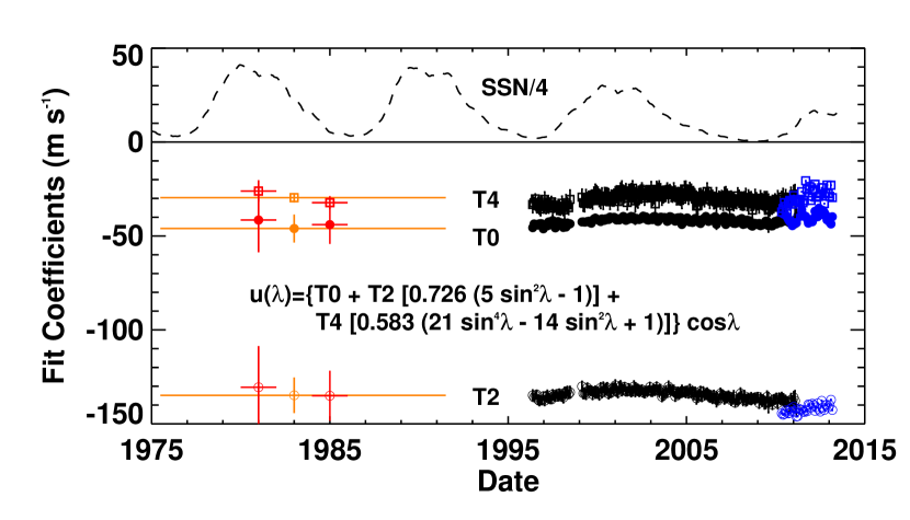
The surface differential rotation varies over the course of each sunspot cycle in small but systematic ways. Changes in the overall shape of the differential rotation can be followed by tracking the changes in the coefficients that fit the profiles. Care should be taken, however, to cast the fits to the profiles in terms of orthogonal polynomials (in this case associated Legendre polynomials of order 1) as was suggested by Snodgrass (1984) to avoid crosstalk between the coefficients. Results of doing this for the measurements made with the small magnetic features are shown in Fig. 3. The average values obtained by Komm et al. (1993b), for the length of their study (1975 to 1991), are shown in orange with 1 error bars for the first three north-south symmetric polynomials (given by the expression included within the figure). Komm et al. (1993b) also provided coefficients for cycle 21 maximum (1980-1982) and for cycle 21/22 minimum (1984-1985). These are shown in red with 1 error bars. The results for individual Carrington rotations, obtained from SOHO/MDI magnetograms by Hathaway and Rightmire (2011), are shown in black with 2 error bars. This is augmented by results from SDO/HMI magnetograms shown in blue with 2 error bars.
All three coefficients are smaller (in absolute terms) at sunspot cycle maxima than they are at cycle minima. This gives a slightly faster (less negative relative to the Carrington rate) solid body rotation but a weaker differential rotation with less latitudinal shear at cycle maxima. The differences in the differential rotation flow profiles between cycle minima and maxima are nonetheless quite small as shown in Fig. 4.
In addition to these systematic changes to the basic profile there are the smaller scale, evolving perturbations referred to as torsional oscillations by Howard and Labonte (1980). These variations in the differential rotation profile are easily seen after removing an average profile (Howe et al., 2011). The deviations from the average profile are in the form of latitude bands with faster and slower than average rotation rates. The faster bands are located on the equatorward sides of the sunspot zones, while the slower bands are located on the poleward sides. This system of fast and slow streams drifts equatorward with the sunspot zones but are apparent at higher latitudes years before sunspots appear. While these flows are clearly associated with the solar cycle and are of considerable interest, the relative flows are quite weak ( m s-1) and thus probably of little consequence for surface flux transport. The torsional oscillations are also seen with helioseismology (Schou et al., 1998) and extend in depth throughout the convection zone (Vorontsov et al., 2002). In addition, helioseismology revealed the existence of a second torsional oscillation branch, which propagates poleward, at high latitudes (Schou, 1999).
4.3 Meridional Circulation
A meridional flow was implicated in surface flux transport long before its strength (or even direction) had been well-determined. In his pioneering paper on the solar dynamo Babcock (1961) suggested that there was a meridional circulation that spread outward from the active latitudes. In his model, the higher latitude poleward flows would transport following polarity flux to the poles where it would reverse the polar fields halfway through the cycle and then build up new polar fields with the sign of the following polarity in each hemisphere. Babcock’s model also included a low latitude equatorward flow that would transport preceding polarity flux to the equator, where it would cancel with the opposite polarity from the other hemisphere. This meridional flow seemed reasonable based on the effects of the Coriolis force on the differential rotation relative to the Carrington rotation frame of reference – the low latitude faster flow would be turned equatorward by the Coriolis force while the high latitude slower flow would be turned poleward. Babcock also cited observations of the motions of sunspots which suggested a meridional flow of this form. After the “discovery” of supergranules by Leighton et al. (1962), Babcock’s meridional circulation was deemed unnecessary by Leighton (1964) who proposed that the surface flux transport was all done by a random walk of the magnetic elements due to evolving granules and supergranules.
The earliest measurements of the meridional flow were based on the motions of sunspot groups. Dyson and Maunder (1913) used sunspot group motions to refine the determination of the orientation of the Sun’s rotation axis and noted a tendency for high latitude groups to move poleward and low latitude groups to move equatorward. Tuominen (1942) examined the meridional motions of recurring sunspot groups (groups that live long enough to be identified on more than one disk passage) and found that these groups did indeed diverge from the active latitudes with velocities of 1-2 m s-1. Similar results were found for individual sunspots by Howard and Gilman (1986). There are two significant problems in using the meridional motions of sunspots in surface flux transport models: sunspots do not appear at high latitudes (thereby leaving the meridional flow unknown poleward of about 40∘) and the motion of sunspots may not representative of the surface meridional flow.
More or less complete latitude coverage is available with direct Doppler, helioseismology, and feature tracking using the small magnetic elements that populate the entire surface of the Sun. Figure 5 shows some of the meridional flow profiles that have been reported. There are small but significant differences in the surface velocity derived from the different techniques. This is partly because the measurements are all subject to systematic uncertainties and sample different depths.
Measurements of the near-surface meridional motions of the small magnetic elements (Komm et al., 1993a; Gizon et al., 2003; Hathaway and Rightmire, 2010; Hathaway and Rightmire, 2011; Rightmire-Upton et al., 2012) can also be used to determine the meridional velocity. A typical cycle-averaged meridional flow profile determined by magnetic feature tracking is as given by Komm et al. (1993a) as
| (9) |
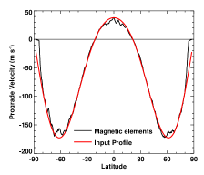
Hathaway and Rightmire (2011) tested the sensitivity of magnetic feature tracking as a way of determining the large-scale flows to the effects of the random motions of the magnetic elements. They took a magnetic map representative of cycle maximum, represented the magnetic field distribution on a 4096-by-1500 grid in longitude and latitude by a collection of some 120,000 magnetic elements that were then advected by an evolving pattern of supergranules. They did not find any substantial flow away from the active latitudes as was suggested by Dikpati et al. (2010). They later (Upton and Hathaway, 2014) produced a fully advective surface flux transport code in which the magnetic elements are transported by the flows in an evolving pattern of supergranules. They assimilate data from magnetograms on the Sun’s near side but the field evolution on the far side is produced purely by the surface flux transport. Figure 6 shows that both the differential rotation and meridional flow measured by magnetic element feature tracking on the far side data for the maximum of cycle 23 (the year 2000) do not differ significantly from the input profiles for this choice of random (supergranular) motions. They argue that the velocity field determined in this way is the most consistent for use in the SFT model.
The interpretation of the Doppler measurements are complicated by the presence of the strong convective blue shift signal (Hathaway, 1996; Ulrich, 2010). This signal is an apparent blue shift in spectral lines due to the correlation between emergent intensity and radial flows in granules. It can vary by as much as 500 m s-1 between disk center and limb, and is affected by the presence of magnetic field (Welsch et al. (2013) studied the Doppler velocity details in active regions and noted that the presence of magnetic fields can have substantial effects on the observed Doppler velocities.). The Doppler signal from the meridional flow has a spatial structure similar to that of the convective blue shift but with a maximum of only 10 m s-1 – hence the difficulty in measuring the meridional flow from the Doppler shift of spectral lines.
Measurements of the meridional flow have been made using several local helioseismic techniques, with similar results for the near-surface flows. The first such measurement (Giles et al., 1997) used the method of time-distance helioseismology (Duvall et al., 1993) and gave a poleward flow of approximately m s-1 at 30∘. More recent near-surface measurements, covering most of cycle 23, are shown in Fig. 7 from two different techniques: MDI time-distance helioseismology measurements of the advection of the supergranulation pattern (Gizon et al., 2003; Gizon and Rempel, 2008) and GONG ring-diagram helioseismology (González Hernández et al., 2008). The peak near-surface meridional velocity is about 15 ms-1 at a latitude of 30∘ in these more recent studies.
The time dependence of the meridional flow is clearly seen in the local helioseismology observations. We see in Fig. 7 that, in the rising phase (1996 to 2002) of the cycle, the latitude where the meridional circulation peaks moves towards lower latitudes. The time-varying component of the near-surface meridional flow is consistent with an inflow into the active latitudes (Gizon, 2004; Zhao and Kosovichev, 2004; Gizon and Rempel, 2008; González Hernández et al., 2010). The inflows into individual active regions can be seen in two dimensional maps, first reported by Gizon et al. (2001) using -mode time-distance helioseismology. A theory for the inflows, related to the enhanced cooling associated with the bright plage, was suggested by Spruit (2003) with a demonstration of the plausibility of the idea being given in Gizon and Rempel (2008).
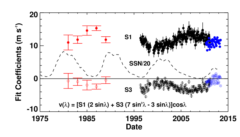
Using magnetic feature tracking applied to MDI observations, Meunier (1999) detected clear changes in the meridional flow associated with active regions. The more extensive MDI measurements of Hathaway and Rightmire (2010) show changes with the solar cycle indicated by: 1) polynomial fits to the profiles (Fig. 8) and 2) by detailed changes to the meridional flow profiles (Hathaway and Rightmire, 2011) fully consistent with superimposed inflows toward the active regions (Cameron and Schüssler, 2010).
5 Sinks of Magnetic Flux
Without the supply of new flux introduced by , the total unsigned flux at the solar surface monotonically decreases. For plausible values of the meridional flow speed and magnetic diffusivity, the e-folding time of the slowest decaying solution is about 4000 years (Cameron and Schüssler, 2007). The slowest decaying solution consists of equal amounts of oppositely directed magnetic flux that is well separated, concentrated at the two poles. Much more rapid decay occurs when the two polarities are close to each other, with an e-folding time of at most a few years as the field of both polarities is advected to the poles where the two polarities then come into close proximity and cancel. The cancellation is, in most models, due to the diffusion term , i.e. it is due to magnetic reconnection which is assumed to occur in the photosphere.
The second type of sink is represented by the term . This type of term was introduced by Schrijver et al. (2002) and Baumann et al. (2006). In physical terms, the idea is that processes below the surface of the Sun, where magnetic diffusion is also operating, cause the magnetic field at the surface to decay in-situ (Baumann et al., 2006). Because both sources and sinks are subject to the same requirement that changes in flux must be localized, Schrijver et al. (2002) suggests the possibility that the decay of the field is accompanied by the emergence of a large number of small, weak bipoles that together form a chain of loops, and allows the field to appear to decay in-situ without violating the argument presented in Section 3. As opposed to emergence events, the decay envisaged here is slow, and the fluxes are low, so that the observational signal of the large chains of bipoles can be lost in the noise of the omnipresent flux recycling.
Because is a parametrisation of the physics of the highly dynamic convection zone, both its functional form and amplitude are open to discussion. Baumann et al. (2006), for example, consider that the functional form of might reflect the eigen solutions of the problem of free-decay in a static convection zone with a uniform diffusivity, which fixes the functional form for the diffusivity. Schrijver et al. (2002), on the other hand, consider a simpler model where the field decays with a constant -folding time.
Once the functional form of is chosen, the question of its amplitude arises. Again this is, in principle, difficult to determine from first principles as it depends on the properties of the turbulence in the convection zone, with mean-field magnetohydrodynamic effects such as turbulent diffusivity and magnetic pumping playing a role. The strength of , in those cases where it has been included, is chosen to ensure that the polar fields reverse during each cycle.
In practical terms, reduces the 4000 year memory of the SFT model to a few cycles. Such a reduction of the memory of the system might be physically justified (as suggested by Schrijver et al., 2002; Baumann et al., 2006), but also has the effect of removing the long term accumulation of small errors in the modeling. For example, Jiang et al. (2011b) used to reduce the effects of the imperfect knowledge and therefore modeling of the source term .
We comment that nonlinearities can be included in the model via the cycle dependence of the latitude and tilt angle at which sunspot groups emerge (Cameron et al., 2010; Jiang et al., 2011b), or the global meridional circulation rate (Wang et al., 2002), or localized inflows into the active region latitudes (Cameron and Schüssler, 2012). Depending on the time being simulated, these nonlinearities can remove the need for a diffusive term to ensure the cyclic reversal of the polar fields and a match with observations.
6 Solar Surface Flux Transport Models
6.1 A reference model
In the above sections, we have presented the observational features of the solar surface flow and the surface flux source due to the BMR emergences. Babcock and Babcock (1955) speculated that the following flux of BMRs tended to migrate poleward, while the leading flux tended to migrate equatorward. The poleward migration of following flux would neutralize and reverse the solar polar fields over the course of a sunspot cycle. Babcock (1961) later speculated that the observed poleward migration might reflect a pattern of meridional flow on the Sun. Leighton (1964) proposed an alternative mechanism – that the random motions of magnetic flux by supergranular flows, together with Joy’s law would lead to a preferred equatorward diffusion of leading flux and poleward diffusion of following flux. This proposal did not require other latitudinal transport mechanisms. However, Mosher (1977) showed that the diffusivity needed by Leighton was much higher than suggested by the observed flows and that a systematic flow was required. From the 1980s onwards such large-scale flows, including differential rotation and meridional flows have been included in the models (DeVore et al., 1984; Sheeley et al., 1985; DeVore, 1987; Wang et al., 1989). A historical review of the development of the surface flux transport model has been given by Sheeley (2005). The models and applications of the magnetic flux transport at the solar surface flux were also reviewed by Mackay and Yeates (2012).
The SFT model (described by Eq. (2)) has been applied to the evolution of the Sun’s global field (see DeVore et al., 1984, and numerous papers there after). It has also been applied (e.g., Schrijver, 2001) to smaller scales, from large active regions to small ephemeral regions. It has been applied by treating the supergranular motions as a diffusivity, as well as by explicitly modeling them (Upton and Hathaway, 2014).
For the differential rotation, the synodic rotation rate of the large-scale magnetic field, as measured by Snodgrass (1983), is widely used in SFT models. It is
| (10) |
For the meridional flow, the profiles
| (11) |
and
| (14) |
are close to the solid curves in Fig.3 at middle and low latitudes. In contrast, a sharp gradient near the equator was used by Wang et al. (1989, 2009). The comparisons of the different profiles are shown in Fig. 11 of Hathaway and Rightmire (2011) and Fig. 3 of Jiang et al. (2013a).
As a reference model, we take the transport equation Eq. (2), with the source in the form of used by van Ballegooijen et al. (1998), transport parameters, i.e., meridional flow and differential rotation in the forms of Eq. (10) and (11), 250 km2s-1 horizontal turbulent diffusivity, and zero radial diffusivity.
6.2 Evolution of an Individual Sunspot Group: Effects of Different Model Parameters
The axisymmetric component of the large-scale field is measured by the axial dipole moment, which is defined as
| (15) |
In this review, we do not consider the equatorial dipole field, which is strongly affected by differential rotation and hence has a short life time, on order of one year (DeVore, 1987). We note that although such a field is not central for the solar cycle evolution of the Sun’s surface field, it is an important ingredient in the evolution of solar open flux (Mackay et al., 2002a; Wang and Sheeley, 2002).
6.2.1 Source Parameters
The initial contribution of an individual BMR with tilt angle and total flux (area ) located at colatitude , to the solar axial dipole field may be expressed as
| (16) |
where is the distance between the opposite polarities. The axial dipole of the bipole then evolves due to the latitudinal transport of the two polarities, which depends on both diffusion and flows. In the presence of diffusion alone, the axial dipole field decays on a time scale (Leighton, 1964; Baumann et al., 2006), which is approximately 30 years for a diffusivity of 250 km2s-1. For the pure advection case, the dipole field is proportional to and declines on the time scale years (Wang and Sheeley, 1991) as both polarities are swept to the poles. In the presence of both systematic flows and diffusion (or random motions) a fraction of the magnetic field can cross the equator (under the action of the diffusive or random motions) after which they are kept apart by the meridional circulation.
Left panel of Fig. 9 from Jiang et al. (2014) shows the combined effect of diffusion and flow on the axial dipole field of a single BMR with area 1000 Hem, total flux 6Mx and a large tilt angle of 80∘ emerged at different latitudes (latitudes 40∘, 30∘, 20∘, 10∘ and 0∘). The BMRs at the high latitudes and close to the equator display quite different dipole field evolution. For the cross-equator emergence (0∘), the centroids of the two polarities are located at about . Advection in each hemisphere separates the polarities and causes the increase of the dipole field. Part (about half) of the flux diffuses and annihilates across the equator along the polarity inversion line (Mackay et al., 2002a). The remaining flux eventually concentrates around the poles and the dipole field reaches a plateau. Jiang et al. (2014) show that the equilibrium axial dipole field generated by the emergence of a single such extreme cross-equatorial BMR is about 20% of the total simulated dipole field generated by all recorded sunspots groups of cycle 17, which had a medium amplitude. When the BMR emerges at 10∘ and 20∘, the poleward flow gradient (larger gradient at lower latitudes) causes an increase of the separation between the polarities and an increase of the dipole field during the beginning phase. Then more leading flux is transported to the same pole and annihilated with the following polarity. This causes a weaker equilibrium field for a BMR emerging at higher latitude. For BMRs emerging at 30∘ and 40∘, the dipole field diminishes in about 2 years. The right panel shows the relation between the final axial dipole field and the latitudinal location of the BMR with a given magnetic flux and tilt angle. The solid curve represents a Gaussian fit with a HWHM in latitude of 8.8∘.
Hence, the large BMRs with large tilt angles emerging close to the equator contribute most to the solar axial dipole field. Usually the BMRs are assumed to obey the Hale’s polarity law in the SFT models. The anti-Hale spots generate the same amplitude of the axial dipole field as the spots obeying Hale’s law, but have opposite sign.
6.2.2 Transport Parameters
Differential rotation is one of the key ingredients in the evolution of the non axisymmetric component of the large-scale magnetic field (DeVore, 1987). It has no effects on the axial dipole field. Hence we do not discuss its effects here.
Figure 10 shows the dependence of the BMR’s axial dipole fields after reaching equilibrium on the diffusivity (left panel) and on the maximum meridional flow strength (right panel). The BMR has 1000 Hem area, 6Mx total flux and normal tilt angle 5∘. We deposit the BMR at 8∘ (dashed line) and 18∘ (solid line) to show the different effects of the diffusion and meridional flow on the BMR eruptions at different latitudes. The reference model is used except for the variations of the diffusivity and the meridional flow strength.
The BMR located at high latitude (18∘) generates higher equilibrium dipole fields at higher diffusivity since more flux from the leading polarity can diffuse across the equator and be transported into the opposite hemisphere. For the BMR located at low latitude (8∘), the axial dipole field increases with the increase of the diffusivity when the diffusivity is low. When the diffusivity is further increased, more flux will be canceled between the two opposite polarities, which causes the decrease of the equilibrium dipole fields. The BMR at a latitude of 8∘ always generates a stronger dipole field than that at 18∘ latitude.
The axial dipole field monotonically decreases to zero with increasing meridional flow when the BMR is deposited at 18∘ latitude. This is because more leading polarity flux is transported to the same pole as the following polarity due to the stronger meridional flow. When the flow is strong enough, all the leading polarity flux is transported to the north pole without diffusion across the equator. When the BMR is deposited at 8∘ latitude, being close to the equator facilitates cross-equator diffusion. When the flow strength is low, more of the flux cancels before the equilibrium dipole field is established. Increasing flow speed decreases the flux cancellation and hence generates a stronger axial dipole field. When the flow is further increased, the flux diffusing across the equator decreases. Hence the axial dipole field decreases. This numerical simulation implies that the variation of the meridional flow might have different effects on the axial dipole field evolution of different cycles since the latitudinal distribution of the sunspot groups depends on the cycle strength (Solanki et al., 2008; Jiang et al., 2011a).
The effects of perturbations to the meridional flow in the form of inflows toward the active latitudes, as described in Section 4.3, on the evolution of solar surface axial dipole field was studied by Jiang et al. (2010b). In each hemisphere, an axisymmetric band of latitudinal flows converging toward the central latitude of the activity belt was superposed onto the background poleward meridional flow. The overall effect of these flow perturbations is to reduce the latitudinal separation of the magnetic polarities of a BMR and thus diminish its contribution to the equilibrium axial dipole field.
6.3 Simulations of Solar Cycles
6.3.1 Comparisons of Observed and Simulated Magnetic Butterfly Diagrams
In his original paper on the transport of solar magnetic flux, Leighton (1964) simulated the effect of the thousands of sources that occur during an entire sunspot cycle. Cycle 21 was the first cycle that permitted a realistic comparison with the observed field (Sheeley et al., 1985; DeVore and Sheeley, 1987; Wang et al., 1989). The observed features of BMRs were derived from the full-disk magnetograms. The large-scale axisymmetric magnetic field features, such as the polar field structure, poleward surges and polar field reversals were well reproduced. The time evolution of the longitudinally averaged photospheric magnetic field, i.e, the magnetic butterfly diagram, is a good illustration of the large-scale field evolution under the flux transport process.
The upper panel of Fig. 11 shows the magnetic butterfly diagram resulting from a flux transport simulation, the source and transport parameters of which are based on Jiang et al. (2010a), see also Schüssler and Baumann (2006). The lower panel of Fig. 11 is produced from the Kitt Peak Solar Observatory synoptic magnetograms of the radial magnetic field. There are qualitative agreements between simulation and observation, particularly concerning the poleward surges of following-polarity magnetic flux leading to the reversals of the polar fields.
Some differences can also be identified between the simulated and the observed magnetic butterfly diagrams. For example, the observations have a more grainy structure, which leads to a high mean flux density at the activity belt, see Eq.(9) of Jiang et al. (2014) for the definition. The average of the observed values over the three cycle maxima is about 3G, which is about twice that of the simulated result. Furthermore, the simulations lack the occasional cross-equatorial flux plumes that appear in the data due to the large, highly tilted sunspot groups that emerge near the equator, for example in the years of 1980, 1986, and 2002 (Cameron et al., 2013).
The differences can mainly be attributed to the scatter in sunspot group tilt angles relative to Joy’s law. Jiang et al. (2014) measured the tilt scatter based on the observed tilt angle data from MWO and Kodaikanal. The standard deviations () of the tilt angles depend on the sunspot area in the form of , where is the umbra area. Figure 12 shows the comparisons of the simulated magnetic butterfly diagrams using the observed sunspot records of cycle 17, which is a cycle with an average strength and not associated with a sudden increase or decrease with respect to the adjacent cycles, without (upper panel) and with (lower panel) the tilt scatter. The lower panel corresponds to one random realization of the sunspot group tilt scatter, which generates the similar polar field as the upper panel without the tilt scatter. The randomly occurring large tilt angles cause the more grainy structure, which is represented by an increase of the low latitude flux density by about 40% compared to the case without tilt angle scatter. There are also more poleward surges with opposite polarities. Qualitatively, the magnetic butterfly diagram for the cases with tilt angle scatter is more similar to the observed counterpart for the last 3 cycles. See Jiang et al. (2014) for more details about the effects of the scatter in sunspot group tilt angles on the magnetic butterfly diagram. Occasionally, the near equator sunspot groups with big sizes have big tilt angles. According to Section 6.2.1, a single such event can significantly affect the axial dipole field at the end of the cycle. If the event obeys the Hale polarity law, it strengthens the axial dipole field. If the event is anti-Hale, it weakens the axial dipole field.
6.3.2 Simulations of Multiple Solar Cycles
The success of the SFT model, with BMR emergence as the main source of flux, opens the possibility for the reconstruction of the solar large-scale magnetic field into the past on the basis of recorded sunspot data. The observed cycle-to-cycle variations provide constraints for the modeling of the different physical processes in the model. When the BMR source amplitude fluctuations were included in the model, Wang et al. (2002) and Schrijver et al. (2002) found that the polar field cannot reverse polarity every 11 yr. In their studies, the BMRs of different cycles had the same range of latitude distributions. The tilt angles of BMRs obeyed Joy’s law and did not depend on the cycle strength. The total intrinsic axial dipole field was proportional to the total flux of the emergent sunspot groups during a cycle. Under the same transport parameters, the strength of the polar field then varied linearly with the total amount of emerged flux. During the weaker cycles the flux supply was insufficient to cancel the existing polar field, to reverse it and to build up a new polar field of opposite polarity and of the same strength as before. Three different ways of resolving this discrepancy have been put forward.
Including in a component due to the intrinsically three-dimensional nature of flux transport
The reference SFT model described in Section 6.1 is explicitly two dimensional. With , there is no flux transport across the solar surface. In models simpler than the SFT, multi-year decay times were proposed by Solanki et al. (2000) to successfully describe the evolution of the total amount of open and total magnetic flux. Schrijver et al. (2002) and Baumann et al. (2006) introduced different forms of in order to account for an intrinsically three-dimensional decay of the field. Schrijver et al. (2002) found that a simple exponential decay of the field with a decay time of about 10 yr allowed regular reversals of the polar fields given fluctuations in the source term similar to those in the historical records. Baumann et al. (2006) introduced a more detailed expression for based on a parameterization of radial diffusion processes. A radial diffusivity of 100 km2s-1 (corresponding to a decay time of 5 years for the dipole component) was suggested. See Section 5 for more discussions.
Nonlinearities in the transport parameters
Variations in the meridional flow have been considered as an alternate way of ensuring the polar fields reverse at the end of each cycle. The two types of changes considered are a modulation of the global flow speed (Wang et al., 2002, 2005), or the inclusion of a localized inflow into active regions (Cameron and Schüssler, 2012). The model of the inflow in the latter study was calibrated to helioseismic observations (Cameron and Schüssler, 2010), although more work is needed to assimilate the raw observations into their model. Both types of nonlinearities can lead to reversals of the polar fields at the end of each cycle.
Nonlinearities in the source parameters
In Section 3 we have listed the characteristics of sunspot group emergence. Strong cycles have a higher mean latitude (related to the Waldmeier effect; Waldmeier 1955) and a lower tilt angle for sunspot emergence (Dasi-Espuig et al., 2010). According to the results discussed in Section 6.2.1, both the latitudes and the tilts of the source term can significantly modulate the polar field generation. Cameron et al. (2010) made the first attempt to introduce nonlinearities in the source parameters to study the magnetic field evolution of multiple cycles. Figure 13 shows the average of the unsigned polar field strength from the flux transport model (red) and observed sunspot area (black). In agreement with observations, the polar field at the end of a solar cycle is correlated with the subsequent cycle strength (e.g., see Muñoz-Jaramillo et al., 2013), and similarly for the open flux (e.g., see Wang and Sheeley, 2009).
Mixed approaches are also possible. Wang and Sheeley (2003) include the nonlinearities in both the source and the transport parameters to simulate the evolution of the Sun’s large-scale magnetic field under Maunder minimum conditions. They showed that the regular polarity oscillations of the axial dipole and polar fields can be maintained if the source flux emerges at low latitudes () and the speed of the poleward surface flow was reduced from to m s-1. Jiang et al. (2011b) have used semi-synthetic records of emerging sunspot groups based on sunspot number data as input for a surface flux transport model to reconstruct the evolution of the large-scale solar magnetic field from the year 1700 onward. A nonlinear modulation of the tilt angles and emergence latitudes based on observations was included as well as a decay term based on the formalism in Baumann et al. (2006) with km2s-1 to reduce the error in the modeling due to the errors in the sunspot numbers. Figure 14 shows the reconstructed polar field based on Wolf sunspot number during 1700-2010 from Jiang et al. (2011b).
6.3.3 Assimilations of Observed Magnetograms
Surface flux transport models have also been used to construct synchronic magnetic maps (maps of the magnetic field over the entire surface of the Sun for a given moment in time) for use in coronal field extrapolations and space weather predictions. In the above sections, the flux sources were idealized as magnetic dipoles produced by the emergence of BMRs. For synchronic map production, observed magnetograms are assimilated into a SFT model that then includes the magnetic field evolution on the far side of the Sun. Worden and Harvey (2000) used their flux transport model and the Kitt Peak synoptic magnetograms to update unobserved or poorly observed regions. Schrijver and De Rosa (2003) assimilated SOHO/MDI magnetograms within 60∘ from disk center into a SFT model with an duration of 5.5 yr and temporal resolution of 6 hours. With this they were able to approximate the evolution of the photospheric magnetic field on the unobservable hemisphere, and thus obtain a continuously evolving model of the surface field over the whole solar surface. Schrijver and Liu (2008) extended the study throughout the whole of cycle 23 to further understand the large-scale transport of the magnetic flux in the solar photosphere. Upton and Hathaway (2014) assimilated magnetograms from both MDI and HMI to produce a “baseline” set of synchronic maps from 1996 to 2013 at a 15-minute cadence for comparison with maps made with BMR sources. They found excellent agreement and showed that predictions of polar field reversals and the polar field strength at cycle minimum could be made years in advance. McCloughan and Durrant (2002) and Durrant and McCloughan (2004) noted that flux transport produces and requires synchronic maps rather than traditional synoptic maps and care must therefore be taken when estimating transport parameters from synoptic maps.
Yeates et al. (2007) used synoptic magnetogram data as the initial condition and assimilated the emergence of new active regions into the model throughout the course of the simulation to maintain the accuracy of the simulated photospheric magnetic field over many months. The simulations were coupled with simulations of the 3 dimensional coronal magnetic field to explain the hemispheric pattern of the axial magnetic field direction in solar filaments (Yeates and Mackay, 2009).
6.4 Peculiar Cycle 23 Minimum
The polar field at the end of cycle 23 was unexpectedly weak, which caused the unusual properties of the polar corona, the open flux, and the solar wind at that time, see Wang et al. (2009) and Jiang et al. (2013a) for more details. As shown in Fig. 15, cycle 23 has a similar amplitude and shape as cycle 17. However, the amplitudes of their subsequent cycles, cycles 24 and 18, are very different. The cycle strength is proportional to the polar field at the end of the preceding cycle (Jiang et al., 2007; Muñoz-Jaramillo et al., 2013), which implies that cycles with similar amplitudes can generate rather different amounts of polar flux at the end of the cycles. This situation poses an interesting challenge to surface flux transport models.
Schrijver and Liu (2008), Wang et al. (2009) and Jiang et al. (2013a) simulated the evolution of the photospheric field of cycle 23 using flux transport models. Sunspot number data were used to determine the number of BMRs emergence at a given time. These studies could produce the observed weak polar field strength by increasing the meridional flow relative to the reference case.
Yeates (2014) simulated cycle 23 by inserting individual BMR with properties matching those in observed Kitt Peak synoptic magnetograms. They also found that their standard flux transport model is insufficient to simultaneously reproduce the observed polar fields and butterfly diagram during cycle 23, and that additional effects must be added. The variations they considered include an increase of the meridional flow to 35 ms-1, decrease of the supergranular diffusivity to 200 km2s-1, decrease of the sunspot groups tilt angle by 20%, decrease of the flux per sunspot groups by 20%, inclusion of in Eq. (1) with a decay time of 5 years, decrease of the tilt angle of the sunspot groups by 20% coupled with radial diffusion in about 10 years, and the inflow toward the active regions.
Stochastic variations in sunspot group emergence is another possible cause of the weak cycle 23 minimum. As shown in Section 6.2.1, large highly tilted BMRs that emerge at low latitudes produce cross-equatorial flux plumes in the synoptic magnetograms and provide a large contribution to the axial dipole field. Cameron et al. (2014) simulated cycles 21-23 and showed that the magnetic flux from four observed cross-equatorial flux plumes could provide one explanation for the weakness of the polar fields at the end of solar cycle 23.
7 Conclusions
The solar photosphere is a thin layer between the high plasma- solar interior and the low plasma- solar atmosphere. It is the layer where the energy transport changes from convective to radiative, the layer where the poloidal field is generated in the Babcock-Leighton model and critically it is the layer that we can observe and best measure the magnetic field. The dynamics of the magnetic field in this layer are, based on observations, particularly simple: emergence, dispersion and advection by surface velocities, and eventually cancellation with opposite polarity flux. These few processes explain the evolution of the large-scale magnetic field at the solar surface, and beyond it in the corona and the heliosphere. In this paper we have reviewed these processes and shown how they can impact the evolution of the Sun’s magnetic field and the sunspot cycle.
The surface flux transport is the key to understanding what produces the polar fields and the axial dipole moment seen at activity minima. The strength of the polar fields at this phase of the activity cycle is well correlated with the strength of the next solar cycle and can be used as a reliable predictor (Schatten et al., 1978; Schatten and Sofia, 1987; Svalgaard et al., 2005; Jiang et al., 2007; Wang and Sheeley, 2009; Muñoz-Jaramillo et al., 2013). In some Babcock-Leighton type dynamo models (e.g., Chatterjee et al., 2004; Jiang et al., 2013b), this correlation exists because the poloidal field generated by the surface flux transport can be quickly transported to the tachocline where it gets wound up by the differential rotation to produce the strong toroidal flux that emerges in the sunspots of the next cycle.
The strength of the polar fields and the axial dipole moment depend on the surface flux transport processes – both the active region sources (total magnetic flux, polarity separation, and latitude of emergence) and the surface flows (differential rotation, meridional flow, and the random convective flows). These processes have been found to vary systematically with both the phase and the strength of sunspot cycles.
The transport processes are dominated by the observed surface flows that include both the large-scale axisymmetric flows (differential rotation and meridional flow) and the smaller scale non-axisymmetric flows (granules, supergranules, giant cells, and flows associated with active regions). These non axisymmetric convective flows are usually treated as diffusion. Some models also include a decay term in addition to the observed surface flows. The combined effects of these transport processes on the emergent sunspot groups impact the Sun’s axial dipole magnetic field in different ways depending on latitude. While high latitude sunspots typically have more latitudinal separation between polarities, sunspots emerging closer to the equator can contribute more to the axial dipole moment by way of cross-equatorial cancelation.
We note that an important aspect of the magnetic flux transport at the solar surface is the natural tendency for perturbations in the sizes of sunspot cycles to produce cycles that continue to grow in size or decay in size (with the inability to reverse the polar fields). On the Sun this tendency must be held in check by some nonlinear feedback mechanism. We discussed some of the possible mechanisms – active region tilt dependent on cycle size, active region latitude distribution dependent on cycle size, variations in the meridional flow dependent on cycle size. At this time it is not clear which, if any, of these mechanisms dominate. It may be that one mechanism limits the growth while another limits the decay and the competition between the two keeps sunspot cycles from exhibiting even more variability.
We now have more that a cycle of reasonably high-resolution and high temporal cadence observations of the magnetic field and the surface flows from SOHO/MDI and SDO/HMI. Extending backwards in time we have over a hundred years of daily records of sunspot group sizes and locations, as well as knowledge of the Sun s open magnetic flux inferred from geomagnetic field measurements (see the review by Svalgaard, this volume). Looking even further back in time, we have sunspot number data extending through the Maunder Minimum. Given this data (and in particular the well-observed transition from large cycle 22 to small cycle 24), we expect that the evolution of the Sun’s large-scale magnetic field is entering a new stage of understanding.
Acknowledgements.
We are grateful to the referee for helpful comments on the paper. We acknowledge the support from ISSI Bern, for our participation in the workshop on the solar activity cycle: physical causes and consequences. J.J. acknowledges the financial support by the National Natural Science Foundations of China (11173033, 11221063, 2011CB811401) and the Knowledge Innovation Program of the CAS (KJCX2-EW-T07). S.K.S. acknowledges the partial support for this work by the BK21 plus program through the National Research Foundation (NRF) funded by the Ministry of Education of Korea. L.G. acknowledges support from DFG SFB 963 Astrophysical Flow Instabilites and Turbulence (Project A18/1) and from EU FP7 Collaborative Project Exploitation of Space Data for Innovative Helio- and Asteroseismology (SPACEINN).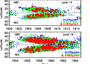


References
- Abramenko (2013) V.I. Abramenko, Fractal multi-scale nature of solar/stellar magnetic fields, in IAU Symposium, ed. by A.G. Kosovichev, E. de Gouveia Dal Pino, Y. Yan IAU Symposium, vol. 294, 2013, pp. 289–300. doi:10.1017/S1743921313002652
- Abramenko et al. (2011) V.I. Abramenko, V. Carbone, V. Yurchyshyn, P.R. Goode, R.F. Stein, F. Lepreti, V. Capparelli, A. Vecchio, Turbulent Diffusion in the Photosphere as Derived from Photospheric Bright Point Motion. Astrophys. J. 743, 133 (2011). doi:10.1088/0004-637X/743/2/133
- Babcock (1961) H.W. Babcock, The Topology of the Sun’s Magnetic Field and the 22-YEAR Cycle. Astrophys. J. 133, 572 (1961). doi:10.1086/147060
- Babcock and Babcock (1955) H.W. Babcock, H.D. Babcock, The Sun’s Magnetic Field, 1952-1954. Astrophys. J. 121, 349 (1955). doi:10.1086/145994
- Balmaceda et al. (2009) L.A. Balmaceda, S.K. Solanki, N.A. Krivova, S. Foster, A homogeneous database of sunspot areas covering more than 130 years. Journal of Geophysical Research (Space Physics) 114, 7104 (2009). doi:10.1029/2009JA014299
- Basu and Antia (2010) S. Basu, H.M. Antia, Characteristics of Solar Meridional Flows during Solar Cycle 23. Astrophys. J. 717, 488–495 (2010). doi:10.1088/0004-637X/717/1/488
- Basu et al. (1999) S. Basu, H.M. Antia, S.C. Tripathy, Ring Diagram Analysis of Near-Surface Flows in the Sun. Astrophys. J. 512, 458–470 (1999). doi:10.1086/306765
- Baumann and Solanki (2005) I. Baumann, S.K. Solanki, On the size distribution of sunspot groups in the Greenwich sunspot record 1874-1976. Astron. Astrophys. 443, 1061–1066 (2005). doi:10.1051/0004-6361:20053415
- Baumann et al. (2006) I. Baumann, D. Schmitt, M. Schüssler, A necessary extension of the surface flux transport model. Astron. Astrophys. 446, 307–314 (2006). doi:10.1051/0004-6361:20053488
- Baumann et al. (2004) I. Baumann, D. Schmitt, M. Schüssler, S.K. Solanki, Evolution of the large-scale magnetic field on the solar surface: A parameter study. Astron. Astrophys. 426, 1075–1091 (2004). doi:10.1051/0004-6361:20048024
- Beck (2000) J.G. Beck, A comparison of differential rotation measurements - (Invited Review). Solar Phys. 191, 47–70 (2000). doi:10.1023/A:1005226402796
- Bogdan et al. (1988) T.J. Bogdan, P.A. Gilman, I. Lerche, R. Howard, Distribution of sunspot umbral areas - 1917-1982. Astrophys. J. 327, 451–456 (1988). doi:10.1086/166206
- Brown et al. (2003) D.S. Brown, R.W. Nightingale, D. Alexander, C.J. Schrijver, T.R. Metcalf, R.A. Shine, A.M. Title, C.J. Wolfson, Observations of Rotating Sunspots from TRACE. Solar Phys. 216, 79–108 (2003). doi:10.1023/A:1026138413791
- Cameron and Schüssler (2007) R. Cameron, M. Schüssler, Solar Cycle Prediction Using Precursors and Flux Transport Models. Astrophys. J. 659, 801–811 (2007). doi:10.1086/512049
- Cameron et al. (2011) R. Cameron, A. Vögler, M. Schüssler, Decay of a simulated mixed-polarity magnetic field in the solar surface layers. Astron. Astrophys. 533, 86 (2011). doi:10.1051/0004-6361/201116974
- Cameron and Schüssler (2010) R.H. Cameron, M. Schüssler, Changes of the Solar Meridional Velocity Profile During Cycle 23 Explained by Flows Toward the Activity Belts. Astrophys. J. 720, 1030–1032 (2010). doi:10.1088/0004-637X/720/2/1030
- Cameron and Schüssler (2012) R.H. Cameron, M. Schüssler, Are the strengths of solar cycles determined by converging flows towards the activity belts? Astron. Astrophys. 548, 57 (2012). doi:10.1051/0004-6361/201219914
- Cameron et al. (2010) R.H. Cameron, J. Jiang, D. Schmitt, M. Schüssler, Surface Flux Transport Modeling for Solar Cycles 15-21: Effects of Cycle-Dependent Tilt Angles of Sunspot Groups. Astrophys. J. 719, 264–270 (2010). doi:10.1088/0004-637X/719/1/264
- Cameron et al. (2012) R.H. Cameron, D. Schmitt, J. Jiang, E. Işık, Surface flux evolution constraints for flux transport dynamos. Astron. Astrophys. 542, 127 (2012). doi:10.1051/0004-6361/201218906
- Cameron et al. (2013) R.H. Cameron, M. Dasi-Espuig, J. Jiang, E. Işık, D. Schmitt, M. Schüssler, Limits to solar cycle predictability: Cross-equatorial flux plumes. Astron. Astrophys. 557, 141 (2013). doi:10.1051/0004-6361/201321981
- Cameron et al. (2014) R.H. Cameron, J. Jiang, M. Schüssler, L. Gizon, Physical causes of solar cycle amplitude variability. Journal of Geophysical Research (Space Physics) 119, 680–688 (2014). doi:10.1002/2013JA019498
- Centeno et al. (2007) R. Centeno, H. Socas-Navarro, B. Lites, M. Kubo, Z. Frank, R. Shine, T. Tarbell, A. Title, K. Ichimoto, S. Tsuneta, Y. Katsukawa, Y. Suematsu, T. Shimizu, S. Nagata, Emergence of Small-Scale Magnetic Loops in the Quiet-Sun Internetwork. Astrophys. J. Lett. 666, 137–140 (2007). doi:10.1086/521726
- Chae et al. (2008) J. Chae, Y.E. Litvinenko, T. Sakurai, Determination of Magnetic Diffusivity from High-Resolution Solar Magnetograms. Astrophys. J. 683, 1153–1159 (2008). doi:10.1086/590074
- Charbonneau (2010) P. Charbonneau, Dynamo Models of the Solar Cycle. Living Reviews in Solar Physics 7, 3 (2010). doi:10.12942/lrsp-2010-3
- Chatterjee et al. (2004) P. Chatterjee, D. Nandy, A.R. Choudhuri, Full-sphere simulations of a circulation-dominated solar dynamo: Exploring the parity issue. Astron. Astrophys. 427, 1019–1030 (2004). doi:10.1051/0004-6361:20041199
- Cheung et al. (2008) M.C.M. Cheung, M. Schüssler, T.D. Tarbell, A.M. Title, Solar Surface Emerging Flux Regions: A Comparative Study of Radiative MHD Modeling and Hinode SOT Observations. Astrophys. J. 687, 1373–1387 (2008). doi:10.1086/591245
- Cheung et al. (2010) M.C.M. Cheung, M. Rempel, A.M. Title, M. Schüssler, Simulation of the Formation of a Solar Active Region. Astrophys. J. 720, 233–244 (2010). doi:10.1088/0004-637X/720/1/233
- Choudhuri (1998) A.R. Choudhuri, The physics of fluids and plasmas : an introduction for astrophysicists (Cambridge University Press, Cambridge, 1998)
- Choudhuri and Gilman (1987) A.R. Choudhuri, P.A. Gilman, The influence of the Coriolis force on flux tubes rising through the solar convection zone. Astrophys. J. 316, 788–800 (1987). doi:10.1086/165243
- Corbard and Thompson (2002) T. Corbard, M.J. Thompson, The subsurface radial gradient of solar angular velocity from MDI f-mode observations. Solar Phys. 205, 211–229 (2002). doi:10.1023/A:1014224523374
- Danilovic et al. (2010) S. Danilovic, B. Beeck, A. Pietarila, M. Schüssler, S.K. Solanki, V. Martínez Pillet, J.A. Bonet, J.C. del Toro Iniesta, V. Domingo, P. Barthol, T. Berkefeld, A. Gandorfer, M. Knölker, W. Schmidt, A.M. Title, Transverse Component of the Magnetic Field in the Solar Photosphere Observed by SUNRISE. Astrophys. J. Lett. 723, 149–153 (2010). doi:10.1088/2041-8205/723/2/L149
- Dasi-Espuig et al. (2010) M. Dasi-Espuig, S.K. Solanki, N.A. Krivova, R. Cameron, T. Peñuela, Sunspot group tilt angles and the strength of the solar cycle. Astron. Astrophys. 518, 7 (2010). doi:10.1051/0004-6361/201014301
- Dasi-Espuig et al. (2013) M. Dasi-Espuig, S.K. Solanki, N.A. Krivova, R. Cameron, T. Peñuela, Sunspot group tilt angles and the strength of the solar cycle (Corrigendum). Astron. Astrophys. 556, 3 (2013). doi:10.1051/0004-6361/201014301e
- de Wijn et al. (2009) A.G. de Wijn, J.O. Stenflo, S.K. Solanki, S. Tsuneta, Small-Scale Solar Magnetic Fields. Space Sci. Rev. 144, 275–315 (2009). doi:10.1007/s11214-008-9473-6
- DeVore (1987) C.R. DeVore, The decay of the large-scale solar magnetic field. Solar Phys. 112, 17–35 (1987). doi:10.1007/BF00148484
- DeVore and Sheeley (1987) C.R. DeVore, N.R. Sheeley Jr., Simulations of the sun’s polar magnetic fields during sunspot cycle 21. Solar Phys. 108, 47–59 (1987). doi:10.1007/BF00152076
- DeVore et al. (1984) C.R. DeVore, J.P. Boris, N.R. Sheeley Jr., The concentration of the large-scale solar magnetic field by a meridional surface flow. Solar Phys. 92, 1–14 (1984). doi:10.1007/BF00157230
- Dikpati et al. (2010) M. Dikpati, P.A. Gilman, R.K. Ulrich, Physical Origin of Differences Among Various Measures of Solar Meridional Circulation. Astrophys. J. 722, 774–778 (2010). doi:10.1088/0004-637X/722/1/774
- Domínguez Cerdeña (2003) I. Domínguez Cerdeña, Evidence of mesogranulation from magnetograms of the Sun. Astron. Astrophys. 412, 65–68 (2003). doi:10.1051/0004-6361:20034617
- Durrant and McCloughan (2004) C.J. Durrant, J. McCloughan, A method of evolving synoptic maps of the solar magnetic field, II. Comparison with observations of the polar fields. Solar Phys. 219, 55–78 (2004). doi:10.1023/B:SOLA.0000021830.88336.86
- Durrant et al. (2001) C.J. Durrant, J.M. Kress, P.R. Wilson, The Evolution of Trailing Plumes from Active Regions. Solar Phys. 201, 57–69 (2001). doi:10.1023/A:1010393806958
- Duvall (1979) T.L. Duvall Jr., Large-scale solar velocity fields. Solar Phys. 63, 3–15 (1979). doi:10.1007/BF00155690
- Duvall et al. (1993) T.L. Duvall Jr., S.M. Jefferies, J.W. Harvey, M.A. Pomerantz, Time-distance helioseismology. Nature 362, 430–432 (1993). doi:10.1038/362430a0
- Dyson and Maunder (1913) F.W. Dyson, E.W. Maunder, Sun, Axis, the position of, from photographs, 1874-1912. Mon. Not. Roy. Astron. Soc. 73, 673 (1913)
- Fan (2009) Y. Fan, Magnetic fields in the solar convection zone. Living Reviews in Solar Physics 6(4) (2009). doi:10.12942/lrsp-2009-4. http://www.livingreviews.org/lrsp-2009-4
- Giles et al. (1998) P.M. Giles, T.L. Duvall Jr., A.G. Kosovichev, ”Solar rotation and large-scale flows determined by time-distance helioseismology MDI”, in New Eyes to See Inside the Sun and Stars, ed. by F.-L. Deubner, J. Christensen-Dalsgaard, D. Kurtz IAU Symposium, vol. 185, 1998, p. 149
- Giles et al. (1997) P.M. Giles, T.L. Duvall, P.H. Scherrer, R.S. Bogart, A subsurface flow of material from the Sun’s equator to its poles. Nature 390, 52–54 (1997). doi:10.1038/36294
- Gizon (2004) L. Gizon, Helioseismology of Time-Varying Flows Through The Solar Cycle. Solar Phys. 224, 217–228 (2004). doi:10.1007/s11207-005-4983-9
- Gizon and Birch (2005) L. Gizon, A.C. Birch, ’local helioseismology’. Living Reviews in Solar Physics 2, 6 (2005). doi:10.12942/lrsp-2005-6
- Gizon and Rempel (2008) L. Gizon, M. Rempel, Observation and Modeling of the Solar-Cycle Variation of the Meridional Flow. Solar Phys. 251, 241–250 (2008). doi:10.1007/s11207-008-9162-3
- Gizon et al. (2010) L. Gizon, A.C. Birch, H.C. Spruit, Local Helioseismology: Three-Dimensional Imaging of the Solar Interior. Annual Review of Astron and Astrophys 48, 289–338 (2010). doi:10.1146/annurev-astro-082708-101722
- Gizon et al. (2003) L. Gizon, T.L. Duvall, J. Schou, Wave-like properties of solar supergranulation. Nature 421, 43–44 (2003). doi:10.1038/nature01287
- Gizon et al. (2001) L. Gizon, T.L. Duvall Jr., R.M. Larsen, Probing Surface Flows and Magnetic Activity with Time-Distance Helioseismology, in Recent Insights into the Physics of the Sun and Heliosphere: Highlights from SOHO and Other Space Missions, ed. by P. Brekke, B. Fleck, J.B. Gurman IAU Symposium, vol. 203, 2001, p. 189
- González Hernández et al. (2008) I. González Hernández, S. Kholikov, F. Hill, R. Howe, R. Komm, Subsurface Meridional Circulation in the Active Belts. Solar Phys. 252, 235–245 (2008). doi:10.1007/s11207-008-9264-y
- González Hernández et al. (2010) I. González Hernández, R. Howe, R. Komm, F. Hill, Meridional Circulation During the Extended Solar Minimum: Another Component of the Torsional Oscillation? Astrophys. J. Lett. 713, 16–20 (2010). doi:10.1088/2041-8205/713/1/L16
- Győri et al. (2011) L. Győri, T. Baranyi, A. Ludmány, ”Photospheric data programs at the Debrecen Observatory”, in IAU Symposium, ed. by D. Prasad Choudhary, K.G. Strassmeier IAU Symposium, vol. 273, 2011, pp. 403–407. doi:10.1017/S174392131101564X
- Hagenaar and Cheung (2009) M. Hagenaar, M. Cheung, Magnetic Flux Emergence on Different Scales, in The Second Hinode Science Meeting: Beyond Discovery-Toward Understanding, ed. by B. Lites, M. Cheung, T. Magara, J. Mariska, K. Reeves Astronomical Society of the Pacific Conference Series, vol. 415, 2009, p. 167
- Hathaway (1996) D.H. Hathaway, Doppler Measurements of the Sun’s Meridional Flow. Astrophys. J. 460, 1027 (1996). doi:10.1086/177029
- Hathaway and Rightmire (2010) D.H. Hathaway, L. Rightmire, Variations in the Sun’s Meridional Flow over a Solar Cycle. Science 327, 1350 (2010). doi:10.1126/science.1181990
- Hathaway and Rightmire (2011) D.H. Hathaway, L. Rightmire, Variations in the Axisymmetric Transport of Magnetic Elements on the Sun: 1996-2010. Astrophys. J. 729, 80 (2011). doi:10.1088/0004-637X/729/2/80
- Hathaway et al. (2013) D.H. Hathaway, L. Upton, O. Colegrove, Giant Convection Cells Found on the Sun. Science 342, 1217–1219 (2013). doi:10.1126/science.1244682
- Hathaway et al. (1996) D.H. Hathaway, P.A. Gilman, J.W. Harvey, F. Hill, R.F. Howard, H.P. Jones, J.C. Kasher, J.W. Leibacher, J.A. Pintar, G.W. Simon, GONG Observations of Solar Surface Flows. Science 272, 1306–1309 (1996). doi:10.1126/science.272.5266.1306
- Howard and Gilman (1986) R. Howard, P.A. Gilman, Meridional motions of sunspots and sunspot groups. Astrophys. J. 307, 389–394 (1986). doi:10.1086/164425
- Howard and Harvey (1970) R. Howard, J. Harvey, Spectroscopic Determinations of Solar Rotation. Solar Phys. 12, 23–51 (1970). doi:10.1007/BF02276562
- Howard and Labonte (1980) R. Howard, B.J. Labonte, The sun is observed to be a torsional oscillator with a period of 11 years. Astrophys. J. Lett. 239, 33–36 (1980). doi:10.1086/183286
- Howard et al. (1984) R. Howard, P.I. Gilman, P.A. Gilman, Rotation of the sun measured from Mount Wilson white-light images. Astrophys. J. 283, 373–384 (1984). doi:10.1086/162315
- Howe (2009) R. Howe, Solar Interior Rotation and its Variation. Living Reviews in Solar Physics 6, 1 (2009). doi:10.12942/lrsp-2009-1
- Howe et al. (2000) R. Howe, J. Christensen-Dalsgaard, F. Hill, R.W. Komm, R.M. Larsen, J. Schou, M.J. Thompson, J. Toomre, Deeply Penetrating Banded Zonal Flows in the Solar Convection Zone. Astrophys. J. Lett. 533, 163–166 (2000). doi:10.1086/312623
- Howe et al. (2011) R. Howe, F. Hill, R. Komm, J. Christensen-Dalsgaard, T.P. Larson, J. Schou, M.J. Thompson, R. Ulrich, The torsional oscillation and the new solar cycle. Journal of Physics Conference Series 271(1), 012074 (2011). doi:10.1088/1742-6596/271/1/012074
- Hoyt and Schatten (1998) D.V. Hoyt, K.H. Schatten, Group Sunspot Numbers: A New Solar Activity Reconstruction. Solar Phys. 181, 491–512 (1998). doi:10.1023/A:1005056326158
- Ishikawa et al. (2010) R. Ishikawa, S. Tsuneta, J. Jurčák, Three-Dimensional View of Transient Horizontal Magnetic Fields in the Photosphere. Astrophys. J. 713, 1310–1321 (2010). doi:10.1088/0004-637X/713/2/1310
- Jafarzadeh et al. (2014) S. Jafarzadeh, S.K. Solanki, A. Lagg, L.R. Bellot Rubio, M. van Noort, A. Feller, S. Danilovic Astron. Astrophys. submitted, (2014)
- Jafarzadeh et al. (2014) S. Jafarzadeh, R.H. Cameron, S.K. Solanki, A. Pietarila, A. Feller, A. Lagg, A. Gandorfer, Migration of ca ii h bright points in the internetwork. Astron. Astrophys. 563, 101 (2014). doi:10.1051/0004-6361/201323011
- Jiang et al. (2014) J. Jiang, R.H. Cameron, M. Schüssler, Effects of the scatter in sunspot group tilt angles on the large-scale magnetic field at the solar surface. Astrophys. J. 791, 5 (2014). doi:10.1088/0004-637X/791/1/5
- Jiang et al. (2007) J. Jiang, P. Chatterjee, A.R. Choudhuri, Solar activity forecast with a dynamo model. Mon. Not. Roy. Astron. Soc. 381, 1527–1542 (2007). doi:10.1111/j.1365-2966.2007.12267.x
- Jiang et al. (2010a) J. Jiang, R. Cameron, D. Schmitt, M. Schüssler, Modeling the Sun’s Open Magnetic Flux and the Heliospheric Current Sheet. Astrophys. J. 709, 301–307 (2010a). doi:10.1088/0004-637X/709/1/301
- Jiang et al. (2010b) J. Jiang, E. Işik, R.H. Cameron, D. Schmitt, M. Schüssler, The Effect of Activity-related Meridional Flow Modulation on the Strength of the Solar Polar Magnetic Field. Astrophys. J. 717, 597–602 (2010b). doi:10.1088/0004-637X/717/1/597
- Jiang et al. (2011a) J. Jiang, R.H. Cameron, D. Schmitt, M. Schüssler, The solar magnetic field since 1700. I. Characteristics of sunspot group emergence and reconstruction of the butterfly diagram. Astron. Astrophys. 528, 82 (2011a). doi:10.1051/0004-6361/201016167
- Jiang et al. (2011b) J. Jiang, R.H. Cameron, D. Schmitt, M. Schüssler, The solar magnetic field since 1700. II. Physical reconstruction of total, polar and open flux. Astron. Astrophys. 528, 83 (2011b). doi:10.1051/0004-6361/201016168
- Jiang et al. (2013a) J. Jiang, R.H. Cameron, D. Schmitt, M. Schüssler, Can Surface Flux Transport Account for the Weak Polar Field in Cycle 23? Space Sci. Rev. 176, 289–298 (2013a). doi:10.1007/s11214-011-9783-y
- Jiang et al. (2013b) J. Jiang, R.H. Cameron, D. Schmitt, E. Işık, Modeling solar cycles 15 to 21 using a flux transport dynamo. Astron. Astrophys. 553, 128 (2013b). doi:10.1051/0004-6361/201321145
- Jin et al. (2009) C. Jin, J. Wang, M. Zhao, Vector Magnetic Fields of Solar Granulation. Astrophys. J. 690, 279–287 (2009). doi:10.1088/0004-637X/690/1/279
- Komm et al. (1993a) R.W. Komm, R.F. Howard, J.W. Harvey, Meridional Flow of Small Photospheric Magnetic Features. Solar Phys. 147, 207–223 (1993a). doi:10.1007/BF00690713
- Komm et al. (1993b) R.W. Komm, R.F. Howard, J.W. Harvey, Rotation rates of small magnetic features from two- and one-dimensional cross-correlation analyses. Solar Phys. 145, 1–10 (1993b). doi:10.1007/BF00627979
- Komm et al. (2003) R. Komm, R. Howe, B.R. Durney, F. Hill, Temporal Variation of Angular Momentum in the Solar Convection Zone. Astrophys. J. 586, 650–662 (2003). doi:10.1086/367608
- Leighton (1964) R.B. Leighton, Transport of Magnetic Fields on the Sun. Astrophys. J. 140, 1547 (1964). doi:10.1086/148058
- Leighton (1969) R.B. Leighton, A Magneto-Kinematic Model of the Solar Cycle. Astrophys. J. 156, 1 (1969). doi:10.1086/149943
- Leighton et al. (1962) R.B. Leighton, R.W. Noyes, G.W. Simon, Velocity Fields in the Solar Atmosphere. I. Preliminary Report. Astrophys. J. 135, 474 (1962). doi:10.1086/147285
- Li and Ulrich (2012) J. Li, R.K. Ulrich, Long-term Measurements of Sunspot Magnetic Tilt Angles. Astrophys. J. 758, 115 (2012). doi:10.1088/0004-637X/758/2/115
- Lites et al. (2008) B.W. Lites, M. Kubo, H. Socas-Navarro, T. Berger, Z. Frank, R. Shine, T. Tarbell, A. Title, K. Ichimoto, Y. Katsukawa, S. Tsuneta, Y. Suematsu, T. Shimizu, S. Nagata, The Horizontal Magnetic Flux of the Quiet-Sun Internetwork as Observed with the Hinode Spectro-Polarimeter. Astrophys. J. 672, 1237–1253 (2008). doi:10.1086/522922
- Mackay and Yeates (2012) D. Mackay, A. Yeates, The Sun’s Global Photospheric and Coronal Magnetic Fields: Observations and Models. Living Reviews in Solar Physics 9, 6 (2012). doi:10.12942/lrsp-2012-6
- Mackay et al. (2002a) D.H. Mackay, E.R. Priest, M. Lockwood, The Evolution of the Sun’s Open Magnetic Flux - I. A Single Bipole. Solar Phys. 207, 291–308 (2002a). doi:10.1023/A:1016249917230
- Mackay et al. (2002b) D.H. Mackay, E.R. Priest, M. Lockwood, The Evolution of the Sun’s Open Magnetic Flux - II. Full Solar Cycle Simulations. Solar Phys. 209, 287–309 (2002b). doi:10.1023/A:1021230604497
- Martinez Pillet et al. (1997) V. Martinez Pillet, B.W. Lites, A. Skumanich, Active Region Magnetic Fields. I. Plage Fields. Astrophys. J. 474, 810 (1997). doi:10.1086/303478
- McCloughan and Durrant (2002) J. McCloughan, C.J. Durrant, A method of evolving synoptic maps of the solar magnetic field. Solar Phys. 211, 53–76 (2002). doi:10.1023/A:1022400324489
- Meunier (1999) N. Meunier, Large-Scale Dynamics of Active Regions and Small Photospheric Magnetic Features. Astrophys. J. 527, 967–976 (1999). doi:10.1086/308111
- Meunier (2005) N. Meunier, Magnetic network dynamics: Activity level, feature size and anchoring depth. Astron. Astrophys. 436, 1075–1086 (2005). doi:10.1051/0004-6361:20042414
- Miesch (2005) M.S. Miesch, Large-Scale Dynamics of the Convection Zone and Tachocline. Living Reviews in Solar Physics 2, 1 (2005). doi:10.12942/lrsp-2005-1
- Mosher (1977) J.M. Mosher, The magnetic history of solar active regions, PhD thesis, California Institute of Technology, Pasadena., 1977
- Muñoz-Jaramillo et al. (2013) A. Muñoz-Jaramillo, M. Dasi-Espuig, L.A. Balmaceda, E.E. DeLuca, Solar Cycle Propagation, Memory, and Prediction: Insights from a Century of Magnetic Proxies. Astrophys. J. Lett. 767, 25 (2013). doi:10.1088/2041-8205/767/2/L25
- Newton and Nunn (1951) H.W. Newton, M.L. Nunn, The Sun’s rotation derived from sunspots 1934-1944 and additional results. Mon. Not. Roy. Astron. Soc. 111, 413 (1951)
- Nordlund et al. (2009) Å. Nordlund, R.F. Stein, M. Asplund, Solar Surface Convection. Living Reviews in Solar Physics 6, 2 (2009). doi:10.12942/lrsp-2009-2
- Parker (1955) E.N. Parker, The Formation of Sunspots from the Solar Toroidal Field. Astrophys. J. 121, 491 (1955). doi:10.1086/146010
- Rempel (2011) M. Rempel, Subsurface Magnetic Field and Flow Structure of Simulated Sunspots. Astrophys. J. 740, 15 (2011). doi:10.1088/0004-637X/740/1/15
- Rieutord and Rincon (2010) M. Rieutord, F. Rincon, The Sun’s Supergranulation. Living Reviews in Solar Physics 7, 2 (2010). doi:10.12942/lrsp-2010-2
- Rightmire-Upton et al. (2012) L. Rightmire-Upton, D.H. Hathaway, K. Kosak, Measurements of the Sun’s High-latitude Meridional Circulation. Astrophys. J. 761, 14 (2012). doi:10.1088/2041-8205/761/1/L14
- Rüdiger et al. (2012) G. Rüdiger, M. Küker, R.S. Schnerr, Cross helicity at the solar surface by simulations and observations. Astron. Astrophys. 546, 23 (2012). doi:10.1051/0004-6361/201219268
- Schatten and Sofia (1987) K.H. Schatten, S. Sofia, Forecast of an exceptionally large even-numbered solar cycle. Geophys. Res. Lett. 14, 632–635 (1987). doi:10.1029/GL014i006p00632
- Schatten et al. (1978) K.H. Schatten, P.H. Scherrer, L. Svalgaard, J.M. Wilcox, Using dynamo theory to predict the sunspot number during solar cycle 21. Geophys. Res. Lett. 5, 411–414 (1978). doi:10.1029/GL005i005p00411
- Scherrer et al. (1995) P.H. Scherrer, R.S. Bogart, R.I. Bush, J.T. Hoeksema, A.G. Kosovichev, J. Schou, W. Rosenberg, L. Springer, T.D. Tarbell, A. Title, C.J. Wolfson, I. Zayer, MDI Engineering Team, The Solar Oscillations Investigation - Michelson Doppler Imager. Solar Phys. 162, 129–188 (1995). doi:10.1007/BF00733429
- Scherrer et al. (2012) P.H. Scherrer, J. Schou, R.I. Bush, A.G. Kosovichev, R.S. Bogart, J.T. Hoeksema, Y. Liu, T.L. Duvall, J. Zhao, A.M. Title, C.J. Schrijver, T.D. Tarbell, S. Tomczyk, The Helioseismic and Magnetic Imager (HMI) Investigation for the Solar Dynamics Observatory (SDO). Solar Phys. 275, 207–227 (2012). doi:10.1007/s11207-011-9834-2
- Schou (1999) J. Schou, Migration of Zonal Flows Detected Using Michelson Doppler Imager F-Mode Frequency Splittings. Astrophys. J. Lett. 523, 181–184 (1999). doi:10.1086/312279
- Schou et al. (1998) J. Schou, H.M. Antia, S. Basu, R.S. Bogart, R.I. Bush, S.M. Chitre, J. Christensen-Dalsgaard, M.P. di Mauro, W.A. Dziembowski, A. Eff-Darwich, D.O. Gough, D.A. Haber, J.T. Hoeksema, R. Howe, S.G. Korzennik, A.G. Kosovichev, R.M. Larsen, F.P. Pijpers, P.H. Scherrer, T. Sekii, T.D. Tarbell, A.M. Title, M.J. Thompson, J. Toomre, Helioseismic Studies of Differential Rotation in the Solar Envelope by the Solar Oscillations Investigation Using the Michelson Doppler Imager. Astrophys. J. 505, 390–417 (1998). doi:10.1086/306146
- Schou et al. (2012) J. Schou, P.H. Scherrer, R.I. Bush, R. Wachter, S. Couvidat, M.C. Rabello-Soares, R.S. Bogart, J.T. Hoeksema, Y. Liu, T.L. Duvall, D.J. Akin, B.A. Allard, J.W. Miles, R. Rairden, R.A. Shine, T.D. Tarbell, A.M. Title, C.J. Wolfson, D.F. Elmore, A.A. Norton, S. Tomczyk, Design and Ground Calibration of the Helioseismic and Magnetic Imager (HMI) Instrument on the Solar Dynamics Observatory (SDO). Solar Phys. 275, 229–259 (2012). doi:10.1007/s11207-011-9842-2
- Schrijver (2001) C.J. Schrijver, Simulations of the Photospheric Magnetic Activity and Outer Atmospheric Radiative Losses of Cool Stars Based on Characteristics of the Solar Magnetic Field. Astrophys. J. 547, 475–490 (2001). doi:10.1086/318333
- Schrijver and De Rosa (2003) C.J. Schrijver, M.L. De Rosa, Photospheric and heliospheric magnetic fields. Solar Phys. 212, 165–200 (2003). doi:10.1023/A:1022908504100
- Schrijver and Liu (2008) C.J. Schrijver, Y. Liu, The Global Solar Magnetic Field Through a Full Sunspot Cycle: Observations and Model Results. Solar Phys. 252, 19–31 (2008). doi:10.1007/s11207-008-9240-6
- Schrijver and Martin (1990) C.J. Schrijver, S.F. Martin, Properties of the large- and small-scale flow patterns in and around AR 19824. Solar Phys. 129, 95–112 (1990). doi:10.1007/BF00154367
- Schrijver et al. (2002) C.J. Schrijver, M.L. De Rosa, A.M. Title, What Is Missing from Our Understanding of Long-Term Solar and Heliospheric Activity? Astrophys. J. 577, 1006–1012 (2002). doi:10.1086/342247
- Schrijver et al. (1996) C.J. Schrijver, R.A. Shine, H.J. Hagenaar, N.E. Hurlburt, A.M. Title, L.H. Strous, S.M. Jefferies, A.R. Jones, J.W. Harvey, T.L. Duvall Jr., Dynamics of the Chromospheric Network: Mobility, Dispersal, and Diffusion Coefficients. Astrophys. J. 468, 921 (1996). doi:10.1086/177747
- Schüssler and Baumann (2006) M. Schüssler, I. Baumann, Modeling the Sun’s open magnetic flux. Astron. Astrophys. 459, 945–953 (2006). doi:10.1051/0004-6361:20065871
- Schüssler and Rempel (2005) M. Schüssler, M. Rempel, The dynamical disconnection of sunspots from their magnetic roots. Astron. Astrophys. 441, 337–346 (2005). doi:10.1051/0004-6361:20052962
- Schüssler and Vögler (2008) M. Schüssler, A. Vögler, Strong horizontal photospheric magnetic field in a surface dynamo simulation. Astron. Astrophys. 481, 5–8 (2008). doi:10.1051/0004-6361:20078998
- Schüssler et al. (1994) M. Schüssler, P. Caligari, A. Ferriz-Mas, F. Moreno-Insertis, Instability and eruption of magnetic flux tubes in the solar convection zone. Astron. Astrophys. 281, 69–72 (1994)
- Sheeley (2005) N.R. Sheeley Jr., Surface Evolution of the Sun’s Magnetic Field: A Historical Review of the Flux-Transport Mechanism. Living Reviews in Solar Physics 2, 5 (2005). doi:10.12942/lrsp-2005-5
- Sheeley et al. (1985) N.R. Sheeley Jr., C.R. DeVore, J.P. Boris, Simulations of the mean solar magnetic field during sunspot cycle 21. Solar Phys. 98, 219–239 (1985). doi:10.1007/BF00152457
- Sivaraman et al. (1993) K.R. Sivaraman, S.S. Gupta, R.F. Howard, Measurement of Kodaikanal white-light images. I - A comparison of 35 years of Kodaikanal and Mount Wilson sunspot data. Solar Phys. 146, 27–47 (1993). doi:10.1007/BF00662168
- Snodgrass (1983) H.B. Snodgrass, Magnetic rotation of the solar photosphere. Astrophys. J. 270, 288–299 (1983). doi:10.1086/161121
- Snodgrass (1984) H.B. Snodgrass, Separation of large-scale photospheric Doppler patterns. Solar Phys. 94, 13–31 (1984). doi:10.1007/BF00154804
- Snodgrass et al. (1984) H.B. Snodgrass, R. Howard, L. Webster, Recalibration of Mount Wilson Doppler measurements (Research note). Solar Phys. 90, 199–202 (1984). doi:10.1007/BF00153796
- Solanki (1989) S.K. Solanki, The origin and the diagnostic capabilities of the Stokes V asymmetry observed in solar faculae and the network. Astron. Astrophys. 224, 225–241 (1989)
- Solanki et al. (2006) S.K. Solanki, B. Inhester, M. Schüssler, The solar magnetic field. Reports on Progress in Physics 69, 563–668 (2006). doi:10.1088/0034-4885/69/3/R02
- Solanki et al. (2000) S.K. Solanki, M. Schüssler, M. Fligge, Evolution of the Sun’s large-scale magnetic field since the Maunder minimum. Nature 408, 445–447 (2000). doi:10.1038/408445a
- Solanki et al. (2008) S.K. Solanki, T. Wenzler, D. Schmitt, Moments of the latitudinal dependence of the sunspot cycle: a new diagnostic of dynamo models. Astron. Astrophys. 483, 623–632 (2008). doi:10.1051/0004-6361:20054282
- Solanki et al. (1996) S.K. Solanki, D. Zufferey, H. Lin, I. Rueedi, J.R. Kuhn, Infrared lines as probes of solar magnetic features. XII. Magnetic flux tubes: evidence of convective collapse? Astron. Astrophys. 310, 33–36 (1996)
- Solanki et al. (2010) S.K. Solanki, P. Barthol, S. Danilovic, A. Feller, A. Gandorfer, J. Hirzberger, T.L. Riethmüller, M. Schüssler, J.A. Bonet, V. Martínez Pillet, J.C. del Toro Iniesta, V. Domingo, J. Palacios, M. Knölker, N. Bello González, T. Berkefeld, M. Franz, W. Schmidt, A.M. Title, SUNRISE: Instrument, Mission, Data, and First Results. Astrophys. J. Lett. 723, 127–133 (2010). doi:10.1088/2041-8205/723/2/L127
- Spruit (2003) H.C. Spruit, Origin of the torsional oscillation pattern of solar rotation. Solar Phys. 213, 1–21 (2003). doi:10.1023/A:1023202605379
- Stein et al. (2011) R.F. Stein, A. Lagerfjärd, Å. Nordlund, D. Georgobiani, Solar Flux Emergence Simulations. Solar Phys. 268, 271–282 (2011). doi:10.1007/s11207-010-9510-y
- Stenflo and Kosovichev (2012) J.O. Stenflo, A.G. Kosovichev, Bipolar Magnetic Regions on the Sun: Global Analysis of the SOHO/MDI Data Set. Astrophys. J. 745, 129 (2012). doi:10.1088/0004-637X/745/2/129
- Svalgaard et al. (2005) L. Svalgaard, E.W. Cliver, Y. Kamide, Sunspot cycle 24: Smallest cycle in 100 years? Geophys. Res. Lett. 32, 1104 (2005). doi:10.1029/2004GL021664
- Thompson et al. (1996) M.J. Thompson, J. Toomre, E.R. Anderson, H.M. Antia, G. Berthomieu, D. Burtonclay, S.M. Chitre, J. Christensen-Dalsgaard, T. Corbard, M. De Rosa, C.R. Genovese, D.O. Gough, D.A. Haber, J.W. Harvey, F. Hill, R. Howe, S.G. Korzennik, A.G. Kosovichev, J.W. Leibacher, F.P. Pijpers, J. Provost, E.J. Rhodes Jr., J. Schou, T. Sekii, P.B. Stark, P.R. Wilson, Differential Rotation and Dynamics of the Solar Interior. Science 272, 1300–1305 (1996). doi:10.1126/science.272.5266.1300
- Tian et al. (2003) L. Tian, Y. Liu, H. Wang, Latitude and Magnetic Flux Dependence of the Tilt Angle of Bipolar Regions. Solar Phys. 215, 281–293 (2003)
- Title et al. (1987) A.M. Title, T.D. Tarbell, K.P. Topka, On the relation between magnetic field structures and granulation. Astrophys. J. 317, 892–899 (1987). doi:10.1086/165339
- Tsuneta et al. (2008) S. Tsuneta, K. Ichimoto, Y. Katsukawa, S. Nagata, M. Otsubo, T. Shimizu, Y. Suematsu, M. Nakagiri, M. Noguchi, T. Tarbell, A. Title, R. Shine, W. Rosenberg, C. Hoffmann, B. Jurcevich, G. Kushner, M. Levay, B. Lites, D. Elmore, T. Matsushita, N. Kawaguchi, H. Saito, I. Mikami, L.D. Hill, J.K. Owens, The Solar Optical Telescope for the Hinode Mission: An Overview. Solar Phys. 249, 167–196 (2008). doi:10.1007/s11207-008-9174-z
- Tuominen (1942) J. Tuominen, Die systematische Strombewegung der Sonnenflecke in heliographischer Breite. Mit 1 Abbildung. Z. Astrophys. 21, 96 (1942)
- Tuominen and Kyrolainen (1982) J. Tuominen, J. Kyrolainen, On the latitude drift of sunspot groups and solar rotation. Solar Phys. 79, 161–172 (1982). doi:10.1007/BF00146980
- Ulrich (2010) R.K. Ulrich, Solar Meridional Circulation from Doppler Shifts of the Fe I Line at 5250 Å as Measured by the 150-foot Solar Tower Telescope at the Mt. Wilson Observatory. Astrophys. J. 725, 658–669 (2010). doi:10.1088/0004-637X/725/1/658
- Ulrich et al. (1988) R.K. Ulrich, J.E. Boyden, L. Webster, S.P. Padilla, H.B. Snodgrass, Solar rotation measurements at Mount Wilson. V - Reanalysis of 21 years of data. Solar Phys. 117, 291–328 (1988). doi:10.1007/BF00147250
- Upton and Hathaway (2014) L. Upton, D.H. Hathaway, Predicting the Sun’s Polar Magnetic Fields with a Surface Flux Transport Model. Astrophys. J. 780, 5 (2014). doi:10.1088/0004-637X/780/1/5
- van Ballegooijen et al. (1998) A.A. van Ballegooijen, N.P. Cartledge, E.R. Priest, Magnetic Flux Transport and the Formation of Filament Channels on the Sun. Astrophys. J. 501, 866 (1998). doi:10.1086/305823
- Verma and Denker (2014) M. Verma, C. Denker, Horizontal flow fields observed in Hinode G-band images IV. Statistical properties of the dynamical environment around pores. ArXiv e-prints (2014)
- Vögler and Schüssler (2007) A. Vögler, M. Schüssler, A solar surface dynamo. Astron. Astrophys. 465, 43–46 (2007). doi:10.1051/0004-6361:20077253
- Vorontsov et al. (2002) S.V. Vorontsov, J. Christensen-Dalsgaard, J. Schou, V.N. Strakhov, M.J. Thompson, Helioseismic Measurement of Solar Torsional Oscillations. Science 296, 101–103 (2002). doi:10.1126/science.1069190
- Waldmeier (1955) M. Waldmeier, Ergebnisse und Probleme der Sonnenforschung. 1955
- Wang and Sheeley (2009) Y.-M. Wang, N.R. Sheeley, Understanding the Geomagnetic Precursor of the Solar Cycle. Astrophys. J. Lett. 694, 11–15 (2009). doi:10.1088/0004-637X/694/1/L11
- Wang and Sheeley (1989) Y.-M. Wang, N.R. Sheeley Jr., Average properties of bipolar magnetic regions during sunspot cycle 21. Solar Phys. 124, 81–100 (1989). doi:10.1007/BF00146521
- Wang and Sheeley (1991) Y.-M. Wang, N.R. Sheeley Jr., Magnetic flux transport and the sun’s dipole moment - New twists to the Babcock-Leighton model. Astrophys. J. 375, 761–770 (1991). doi:10.1086/170240
- Wang and Sheeley (2002) Y.-M. Wang, N.R. Sheeley Jr., Sunspot activity and the long-term variation of the Sun’s open magnetic flux. Journal of Geophysical Research (Space Physics) 107, 1302 (2002). doi:10.1029/2001JA000500
- Wang and Sheeley (2003) Y.-M. Wang, N.R. Sheeley Jr., Modeling the Sun’s Large-Scale Magnetic Field during the Maunder Minimum. Astrophys. J. 591, 1248–1256 (2003). doi:10.1086/375449
- Wang et al. (2002) Y.-M. Wang, J. Lean, N.R. Sheeley Jr., Role of a Variable Meridional Flow in the Secular Evolution of the Sun’s Polar Fields and Open Flux. Astrophys. J. Lett. 577, 53–57 (2002). doi:10.1086/344196
- Wang et al. (2005) Y.-M. Wang, J.L. Lean, N.R. Sheeley Jr., Modeling the Sun’s Magnetic Field and Irradiance since 1713. Astrophys. J. 625, 522–538 (2005). doi:10.1086/429689
- Wang et al. (1989) Y.-M. Wang, A.G. Nash, N.R. Sheeley Jr., Evolution of the sun’s polar fields during sunspot cycle 21 - Poleward surges and long-term behavior. Astrophys. J. 347, 529–539 (1989). doi:10.1086/168143
- Wang et al. (2009) Y.-M. Wang, E. Robbrecht, N.R. Sheeley Jr., On the Weakening of the Polar Magnetic Fields during Solar Cycle 23. Astrophys. J. 707, 1372–1386 (2009). doi:10.1088/0004-637X/707/2/1372
- Wang et al. (2002) Y.-M. Wang, N.R. Sheeley Jr., J. Lean, Meridional Flow and the Solar Cycle Variation of the Sun’s Open Magnetic Flux. Astrophys. J. 580, 1188–1196 (2002). doi:10.1086/343845
- Ward (1966) F. Ward, Determination of the Solar-Rotation Rate from the Motion of Identifiable Features. Astrophys. J. 145, 416 (1966). doi:10.1086/148783
- Weber et al. (2011) M.A. Weber, Y. Fan, M.S. Miesch, The Rise of Active Region Flux Tubes in the Turbulent Solar Convective Envelope. Astrophys. J. 741, 11 (2011). doi:10.1088/0004-637X/741/1/11
- Weber et al. (2013) M.A. Weber, Y. Fan, M.S. Miesch, Comparing Simulations of Rising Flux Tubes Through the Solar Convection Zone with Observations of Solar Active Regions: Constraining the Dynamo Field Strength. Solar Phys. 287, 239–263 (2013). doi:10.1007/s11207-012-0093-7
- Weiss and Thompson (2009) N.O. Weiss, M.J. Thompson, The Solar Dynamo. Space Sci. Rev. 144, 53–66 (2009). doi:10.1007/s11214-008-9435-z
- Welsch et al. (2013) B.T. Welsch, G.H. Fisher, X. Sun, A Magnetic Calibration of Photospheric Doppler Velocities. Astrophys. J. 765, 98 (2013). doi:10.1088/0004-637X/765/2/98
- Wolf (1861) R. Wolf, Abstract of his latest Results. Mon. Not. Roy. Astron. Soc. 21, 77 (1861)
- Worden and Harvey (2000) J. Worden, J. Harvey, An Evolving Synoptic Magnetic Flux map and Implications for the Distribution of Photospheric Magnetic Flux. Solar Phys. 195, 247–268 (2000). doi:10.1023/A:1005272502885
- Yeates (2014) A.R. Yeates, Coronal Magnetic Field Evolution from 1996 to 2012: Continuous Non-potential Simulations. Solar Phys. 289, 631–648 (2014). doi:10.1007/s11207-013-0301-0
- Yeates and Mackay (2009) A.R. Yeates, D.H. Mackay, Modelling the Global Solar Corona: III. Origin of the Hemispheric Pattern of Filaments. Solar Phys. 254, 77–88 (2009). doi:10.1007/s11207-008-9276-7
- Yeates et al. (2007) A.R. Yeates, D.H. Mackay, A.A. van Ballegooijen, Modelling the Global Solar Corona: Filament Chirality Observations and Surface Simulations. Solar Phys. 245, 87–107 (2007). doi:10.1007/s11207-007-9013-7
- Zhao and Kosovichev (2004) J. Zhao, A.G. Kosovichev, Torsional Oscillation, Meridional Flows, and Vorticity Inferred in the Upper Convection Zone of the Sun by Time-Distance Helioseismology. Astrophys. J. 603, 776–784 (2004). doi:10.1086/381489
- Zhao et al. (2004) J. Zhao, A.G. Kosovichev, T.L. Duvall Jr., On the Relationship between the Rotational Velocity and the Field Strength of Solar Magnetic Elements. Astrophys. J. Lett. 607, 135–138 (2004). doi:10.1086/421974
- Zhao et al. (2013) J. Zhao, R.S. Bogart, A.G. Kosovichev, T.L. Duvall Jr., T. Hartlep, Detection of Equatorward Meridional Flow and Evidence of Double-cell Meridional Circulation inside the Sun. Astrophys. J. Lett. 774, 29 (2013). doi:10.1088/2041-8205/774/2/L29