A coupled D Babcock–Leighton solar dynamo model. II. Reference dynamo solutions
Abstract
In this paper we complete the presentation of a new hybrid D flux transport dynamo (FTD) model of the solar cycle based on the Babcock–Leighton mechanism of poloidal magnetic field regeneration via the surface decay of bipolar magnetic regions (BMRs). This hybrid model is constructed by allowing the surface flux transport (SFT) simulation described in Lemerle et al. (2015) to provide the poloidal source term to an axisymmetric FTD simulation defined in a meridional plane, which in turn generates the BMRs required by the SFT. A key aspect of this coupling is the definition of an emergence function describing the probability of BMR emergence as a function of the spatial distribution of the internal axisymmetric magnetic field. We use a genetic algorithm to calibrate this function, together with other model parameters, against observed cycle 21 emergence data. We present a reference dynamo solution reproducing many solar cycle characteristics, including good hemispheric coupling, phase relationship between the surface dipole and the BMR-generating internal field, and correlation between dipole strength at cycle maximum and peak amplitude of the next cycle. The saturation of the cycle amplitude takes place through the quenching of the BMR tilt as a function of the internal field. The observed statistical scatter about the mean BMR tilt, built into the model, acts as a source of stochasticity which dominates amplitude fluctuations. The model thus can produce Dalton-like epochs of strongly suppressed cycle amplitude lasting a few cycles and can even shut off entirely following an unfavorable sequence of emergence events.
Subject headings:
dynamo — Sun: activity — Sun: interior — Sun: magnetic fields — Sun: photosphere — sunspotsI. Introduction
Close to a century has now gone by since the discovery of the underlying magnetic nature of the eleven-year sunspot cycle (Hale et al., 1919). The magnetic polarity reversals of the leading and following (with respect to rotation) components of large bipolar magnetic regions is now thought to reflect the presence, somewhere in the solar interior, of a large-scale, dominantly axisymmetric zonally-oriented (toroidal) magnetic field, antisymmetric about the sun’s equator and itself undergoing polarity reversals approximately every eleven years, for a full magnetic cycle period of years. The rotational shear of a pre-existing dipole, later detected on the solar surface (Babcock & Babcock, 1955), can act as an inductive source for such an internal toroidal magnetic flux system. However, closing the dynamo loop requires an inductive mechanism capable of regenerating the dipole from this internal toroidal component, in a manner such as leading the cyclic polarity reversals of both of these large-scale components of the solar magnetic field.
Many candidates for this toroidal-to-poloidal hydromagnetic inductive mechanisms have been identified, starting with cyclonic convection (Parker, 1955) and its associated mean electromotive force, and the surface decay of bipolar magnetic regions (Babcock, 1961), now referred to as the Babcock–Leighton (BL) mechanism. These were joined more recently by helical waves along thin magnetic flux tubes (Schmitt 1987; Ossendrijver 2000, and references therein), and shear instabilities in the tachocline (Dikpati & Gilman, 2001), the stably stratified rotational shear layer located beneath the base of the solar convection zone, as revealed by helioseismology. In all cases, the rotational influence mediated by the Coriolis force is the key agent that breaks the mirror symmetry of the inductive flows, thus allowing to circumvent Cowling’s theorem.
Of these various candidates for poloidal field regeneration, the BL mechanism stands out as the only one that can be directly observed operating at the solar surface, and as such is far better constrained than any other. In particular, the distribution of tilt angles of BMRs, namely the angle defined by a line segment joining each pole of the BMR measured with respect to the east–west direction, is now well characterized from white light (Howard, 1991; Dasi-Espuig et al., 2010) and magnetographic observations (Wang & Sheeley, 1989). This tilt arises through the action of the Coriolis force, and associated with it is a net dipole moment so that, effectively, a poloidal magnetic component is being produced from the pre-existing deep-seated toroidal component ultimately giving rise to emerging BMRs (see Fan 2009 for a review). The magnitude of this tilt, and its pattern of variations with latitude, BMR flux and separation, and statistical fluctuations about the mean, all play a key role in setting the magnitude of the surface dipole moment produced in the course of a sunspot cycle.
Because the BL mechanism operates at the solar surface, a transport mechanism is also needed to carry the surface poloidal magnetic field down into the interior, where rotational shearing is taking place. Here again a number of appropriate candidate mechanisms are available, including advection by large-scale meridional flows pervading the solar convection zone, as well as turbulent transport effects, namely isotropic diffusive transport and directional turbulent pumping. Viewed globally, the BL mechanism is a non-local inductive effect: the surface source of poloidal field is driven by the deep-seated toroidal component, on timescales much shorter than the magnetic cycle period.
Dynamo models of the solar cycle relying on the BL mechanism of poloidal field regeneration have undergone a vigorous revival in the last 25 years or so, spurred by Wang et al. (1989), Wang & Sheeley (1991), Choudhuri et al. (1995), and Durney (1995). Many such models are now dispersed in the literature (for recent reviews see Charbonneau 2010; Karak et al. 2014). The vast majority rely on a two-dimensional axisymmetric formulation of the problem, whereby the large-scale flows and magnetic field components are both axisymmetric, and the dynamo equations solved in a meridional plane. Typically, helioseismology-compatible parameterizations for solar-like internal differential rotation and meridional circulation are introduced, and these flows are assumed steady (the so-called kinematic approximation).
Many such models do differ in how they incorporate the BL mechanism, a fundamentally non-axisymmetric effect, into the axisymmetric dynamo equations (compare, e.g., Durney 1995; Dikpati & Charbonneau 1999; Nandy & Choudhuri 2001; Muñoz-Jaramillo et al. 2010). They also differ in assumptions made regarding the primary magnetic field transport mechanism. As a consequence, models based on rather different input physics can do roughly as well as one another in reproducing the primary characteristics of the observed solar cycle. However, the differences can matter a lot in practice. Perhaps no better illustration of this point can be found than the widely differing dynamo model-based predictions of sunspot cycle 24 made by Dikpati et al. (2006) and Choudhuri et al. (2007), each using a distinct BL model “calibrated” to earlier sunspot cycles.
This problem is compounded when introducing data assimilation into the model-based prediction, as the datasets must then also be preprocessed in some way to accommodate the axisymmetric formulation of the dynamo model used for forecasting. Both aforecited model-based prediction schemes used distinct geometrically simplified implementations of different datasets being assimilated, and in all likelihood these differences also contributed to the widely varying predictions for the amplitude of cycle 24. Ideally, data assimilation should be carried out using full-disk magnetograms and/or detailed observations of active region emergences, including complete positional and timing information. Either way, this requires a dynamo model with a geometrically complete representation of the solar surface, and thus demands abandoning axisymmetry.
One extreme possibility consists in turning to global magnetohydrodynamical simulations of solar convection. Despite remarkable progress in the past decade (for a review see, e.g., § 3 of Charbonneau 2014), such simulations still cannot accommodate sufficient spatial resolution to resolve convection and magnetic field evolution in the surface layers, or even capture the interior process of magnetic flux rope formation and buoyant rise (but on the latter do see Fan & Fang 2014; Nelson et al. 2013; 2014). Typically, such simulations also fail to drive regular, solar-like polarity cyclic reversals in the large-scale magnetic field they generate (see Passos & Charbonneau 2014 for the closest thing yet).
Intermediate approaches are also possible: finding a way to include the full non-axisymmetric representation of, at-least, the surface processes, while retaining the kinematic approach for the transport of magnetic flux. To our knowledge, only two such models exist in the literature (Yeates & Muñoz-Jaramillo, 2013; Miesch & Dikpati, 2014, hereafter MD2014), as they include a full three-dimensional kinematic representation of the solar convection zone up to the surface. Here again, they mostly differ in how they incorporate the localized emergence of new magnetic flux: Yeates & Muñoz-Jaramillo (2013) impose localized flow perturbations at the base of the convection zone to trigger the eruption of active regions out of the toroidal flux, while MD2014 and Miesch & Teweldebirhan (2015) apply a surface flux deposition technique, through an empirical masking of the deep-seated toroidal field.
In this series of paper we present a BL dynamo model that belongs to this same category. We retain a fairly conventional two-dimensional axisymmetric kinematic flux transport dynamo (FTD) model, specifically the model described in Charbonneau et al. (2005), without its non-local poloidal source term, and couple it to a two-dimensional surface flux transport (SFT) simulation. The latter provides the source term for the former through the upper boundary condition, and in turn the FTD provides the emergences required as input to the SFT simulation. We opted to call this a “D” dynamo model. This is still a kinematic model, in that it uses steady parametrized large-scale flow fields compatible with helioseismology and surface measurements. Specifying the form of these flows requires the adjustment of many model parameters, in order to generate the most “solar-like” dynamo solutions possible.
In Lemerle et al. (2015, hereafter Paper I) we introduced a genetic algorithm-based method for formally carrying out this optimization problem, in the context of the surface flux transport simulation. The optimization process is set to minimize deviations with respect to synoptic magnetograms (and derived global quantities). Not only does this approach finds an optimal solution, but it also allows to map a range of acceptable solutions, thus providing robust Monte Carlo-like confidence intervals on best-fit model parameters and allowing the identification of parameter degeneracies. A key result is that the range of acceptable surface meridional flow profiles fits nicely surface Doppler measurements (Ulrich, 2010), even though these data are not used to constrain the optimization process.
In the present paper we extend the procedure to the coupled model described above, and thus produce an “optimal” D BL dynamo model of the solar cycle. The use of quotes is motivated by the fact that even this basic optimal model involves unavoidable stochastic components, associated with the flux emergence process, so that it can only fit the Sun (meaning, e.g., the sunspot number time series) in a statistical sense. Indeed, the SFT solutions presented in Paper I already show how the uncertainties in global cycle characteristics are dominated by the inherent stochasticity of the flux emergence process.
In § 2 we discuss the formulation of the coupled model and its components. In § 3 we turn to its calibration against observed solar features. In § 4 we present self-consistent reference dynamo solutions and examine their patterns of long term variability. In § 5 we discuss the limitations of the calibration technique and compare some of the results with direct solar observations. We conclude by summarizing our most salient results as well as possible paths of improvement and ongoing work.
II. Model
The contemporary version of the original scenario proposed by Babcock (1959) runs as follows:
-
(0)
at solar maximum, strong toroidal magnetic fields are present deep in the solar interior, antisymmetric with respect to the equator;
-
(i)
during the ascending and descending phases of the solar cycle, toroidal flux loops rise and emerge at the solar surface in the form of BMRs, twisted due to the Coriolis effect, such that the western spots tend to be closer to the equator (tilt following on average Joy’s law);
-
(ii)
surface diffusion/transport near the equator allows for more cancellation of the western polarities, when merging with their counterparts from the other hemisphere, leaving the remaining “eastern” flux to be transported toward the poles and trigger the polarity reversal of magnetic polar caps;
-
(iii)
the new surface dipole is subducted and sheared by differential rotation, building up a new internal toroidal magnetic structure, opposite to the preceding one and ready for…
-
(iv)
…the generation of a new population of BMRs during the next half-cycle (from now on, we refer to such half magnetic cycle, or sunspot cycle, as simply a “cycle”).
The numerical implementation we propose for carrying out this scheme is quite simple:
-
(i)
new BMRs are continuously deposited at the solar surface, at times, latitudes and longitudes, tilts, angular separations, magnetic fluxes and polarity generated through a (probabilistic) flux emergence algorithm based on the strength and spatial distribution of the deep-seated magnetic fields;
-
(ii)
the SFT equation is solved on the solar spherical surface, and generates the expected cancellation, decay, transport and specific features typically observed in surface magnetograms (see Paper I);
-
(iii)
the FTD equation is solved in the meridional plane, using the evolving results of the surface simulation as a time-dependent upper boundary condition on the poloidal field; transport of this poloidal field to the base of the convection zone and subsequent shearing by differential rotation eventually builds up strong toroidal magnetic fields deep in the convection zone;
-
(iv)
the dynamo loop is closed by allowing this deep-seated magnetic structure to generate the emergences required in step (i).
II.1. Basic Ingredients
In the depths of the solar convection zone or in the tangles of photospheric turbulent motions, magnetic fields are dispersed, transported, amplified or destroyed by small and large-scale flows. In the solar interior and photosphere, these processes are well-captured by the magnetohydrodynamics (MHD) induction equation:
| (1) |
with the net magnetic diffusivity, including contributions from the small microscopic magnetic diffusivity (with the electric resistivity of the plasma), as well as a dominant turbulent contribution associated with the destructive folding of magnetic field lines by small-scale convective fluid motions. We adopt here the kinematic approximation, whereby the flow u is considered given. This approximation has been shown to be appropriate in reproducing reasonably well the synoptic evolution of the solar surface magnetic field (see, e.g., Wang et al., 2002a; Baumann et al., 2004), as well as the overall solar dynamo properties (see, e.g., Karak et al., 2014, and references therein). On spatial scales much larger than convection, two flows contribute to u: meridional circulation and differential rotation . Both these flows can be considered axisymmetric () and steady () as per the kinematic approximation. They can be expressed in spherical polar coordinates as
| (2) |
where the meridional flow has been formulated in terms of a stream function , thus ensuring mass conservation in a density profile, with , for an adiabatic stratification, the solar radius, and .
II.1.1 Meridional Circulation
We opted to use a modified form of the meridional flow profile introduced by van Ballegooijen & Choudhuri (1988). This flow can be defined through a separable stream function of the form:
| (3a) | ||||||
| where | ||||||
| and . Parameters and determine the depth and concentration of the return flow, down to . For the purpose of the foregoing analysis and calibration, parameters and will be treated as free parameters, while the polytropic index is set at , appropriate for an adiabatic stratification. | ||||||
We deviate from the original formulation of van Ballegooijen & Choudhuri (1988) by using the following latitudinal dependence, also used in Paper I:
| (3b) |
with a normalization factor such that is the maximum meridional flow velocity and , , , and parameters that allow to generate a very wide range of solar-like surface meridional flow profiles. The value of is fixed to as to prevent the formation of a plateau near the equator. We developed this flexible formulation in Paper I to allow for the inclusion of various profiles used in flux transport modeling (e.g., Dikpati & Charbonneau 1999; van Ballegooijen & Choudhuri 1988; Wang et al. 2002b) and measured on the Sun (e.g., Ulrich 2010).
II.1.2 Differential Rotation
Unlike meridional circulation, the solar internal differential rotation profile is well constrained by helioseismology. We use here the helioseismically-calibrated solar-like parameterization introduced in Charbonneau et al. (1999):
| (4a) | |||
| with , , and surface rotation | |||
| (4b) | |||
where , , and (see also Snodgrass 1983). The thickness of the transition region between differential and solid rotation, the tachocline, near the base of the convection zone, is kept as a free parameter.
II.1.3 Magnetic Diffusivity
In the stably stratified core, the presumed absence of turbulence suggests a net diffusivity () given by Ohmic dissipation, while in the bulk of the convection zone, enhanced turbulent dissipation () of the magnetic field is expected to dominate. The following parametric profile, given by Dikpati & Charbonneau (1999), allows for a smooth transition between these two regimes:
| (5) |
where takes the same value as in the preceding differential rotation profile.
In the surface layer, supergranular convective motions drive a random walk that disperses magnetic flux, and can be modeled as a diffusive process (Leighton, 1964) characterized by an effective magnetic diffusivity of order . This value is used solely in the SFT part of the model. The overall radial profile of consequently includes an implicit step function at . The exact values for , , and , as well as , are virtually impossible to determine from first principles, such that they must be treated as unknown parameters needing a proper calibration.
II.2. The Flux Transport Dynamo Equations
The large-scale axisymmetric magnetic field simulated in the FTD component of the model can be expressed as
| (6) |
where and are respectively the poloidal and toroidal vector components of the field. Inserting this decomposition for B, along with Equation (2) for the flow, into the MHD induction Equation (1) then yields the usual two evolutionary equations for the scalar components and :
| (7a) | ||||
| (7b) | ||||
These two equations are linear in and , but are coupled by the shearing term in Equation (7b) which acts as a source for proportional to . No such source appears explicitly in Equation (7a). Here the regeneration and amplification of the poloidal field is supplied by a continuous input from the SFT simulation, providing a time-evolving surface boundary condition for which effectively acts as a source.
II.3. Surface Flux Transport
Following earlier modeling work on surface magnetic flux evolution, in particular in Paper I, we consider the magnetic field to be predominantly radial on global scales and we solve only the -component of Equation (1), at . This leads to the usual two-dimensional linear advection–diffusion equation for the scalar component ,
| (8) |
to which two supplementary terms have been added: a source term to account for the discrete emergence of new surface flux in the form of BMRs, and a linear sink term to allow for an exponential decay of the surface field with time. Schrijver et al. (2002) originally found such a decay on a timescale of to be necessary to preclude secular drift and ensure polarity reversal of the polar caps when modeling surface flux evolution over many successive cycles of differing amplitudes. This was subsequently justified physically by Baumann et al. (2006) as the effect of a vertical turbulent diffusion, or equivalently a convective submergence, on the decay of the dominant dipole mode, two physical mechanisms that cannot be directly included in the SFT model. We included this term in Paper I but did not find it to be required for the SFT results to match the synoptic magnetogram of cycle 21. We test it again here, with treated as a free parameter.
II.4. Numerical Solution and Coupling
The FTD equations (7) and SFT equation (8) are solved concurrently, each on a separate two-dimensional computational grid on which spatial discretization is carried out via the Galerkin finite element method, and implicit temporal discretization through the one-step -method (see, e.g., Burnett 1987).
The SFT simulation is solved over a regular Cartesian grid in representing the whole solar surface, with longitudinal periodicity enforced through a padding of ghost cells. Rigorous flux conservation is also required since only a small fraction of the emerging magnetic flux ultimately builds up the axial dipole observed at sunspot minima. We minimize numerical discretization errors by adopting double precision arithmetics, a longitude–latitude grid, and time steps for the eight-cycle runs that will be analyzed in § 3 (for more details on numerical errors see Paper I, § 2.4 and discussion therein).
The FTD simulation is solved simultaneously over a regular Cartesian grid in (,), from pole to pole and . Below , the radiative core is considered perfectly conductive and the boundary condition is applied. For , the absence of flows and electrical currents imposes . The spherical geometry finally constrains at the poles. The overall scheme is similar to that described in Charbonneau et al. (2005).
With such spatial resolutions and typical time steps of and days respectively in the SFT and FTD simulations, the former dominates the computational workload by a factor of .
II.4.1 From SFT to FTD
The surface () boundary condition on is updated at every FTD time step, via the longitudinal averaging of the SFT solution and integration of the resulting latitudinal function:
| (9) |
where is set to zero at the poles. This provides the coupling from the SFT toward the FTD model.
Such coupling assumes that physical processes responsible for surface magnetic flux evolution occur only inside the single FTD grid layer located at , which is of thickness for our working spatial mesh.
II.4.2 From FTD to SFT: Emergence Function
The coupling from the FTD toward the SFT is the emergence of BMRs. In view of the considerable complexity of the various processes involved in the formation, destabilization, buoyant rise, and emergence of deep-seated magnetic flux tubes (see, e.g., Weber et al. 2011 and review by Fan 2009), we opted here to input emerging BMRs directly into the SFT component of the model, based on a semi-empirical emergence function giving, as a function of the strength of the internal magnetic field, the probability that the emergence of a BMR will occur.
Calculations of the destabilization and buoyant rise of magnetic flux tubes carried out in the thin-tube approximation do offer some useful guidance. From the stability diagrams obtained by Schüssler et al. (1994) and Ferriz-Mas et al. (1994), one can infer the depth, latitude and magnetic amplitudes at which toroidal flux tubes are expected to destabilize. According to their results, and depending on the level of subadiabaticity in the outer reaches of the radiative core, instability growth rates near remain approximately constant, or show a smooth increase with latitude, from the equator up to , and then fall of rapidly to zero over a latitudinal width of . A lower threshold of order is also required, on the amplitude of the magnetic field inside concentrated flux tubes. A crucial missing link is the degree of magnetic field amplification taking place during the formation of these toroidal flux tubes from the dynamo-generated large-scale magnetic field. Accordingly, we define this lower limit as (with units that depend on the exact parameterization of Equation 10 below), and treat it as another free parameter to be calibrated. Modeling also shows that a certain level of twist is required for the tube to maintain its coherence during the rise through the convective envelope (Fan, 2009). Accordingly, we introduce the quantity , evaluated at depth and with exponents in the ranges and , and use it to build the following quasi-normalized emergence function:
| (10) |
The first part of Equation (10) sets a lower threshold on above which emergences can take place, as well as a possible saturation () or linear growth () of the probability above . The transition scale is set to some fraction of (see § III). The second part accounts for the latitudinal dependence of the instability’s growth rate, which we assume to increase linearly from at the equator to near latitude , followed by a quick drop to zero in (cf. Figures 1 and 2 of Ferriz-Mas et al. 1994). The sign of is given by the sign of the input .
The emergence process is made inherently non-deterministic with the following sources of stochasticity:
- (i)
-
(ii)
the probability of emergence of a BMR at a given latitude is made proportional to .
Also, independently from the distribution of , and as determined in our analysis of Wang & Sheeley (1989)’s database entries (see Appendix A of Paper I):
-
(iii)
emergence longitudes are assumed to be random;
-
(iv)
magnetic fluxes are extracted from a log-normal distribution centered at with standard deviation (Paper I, Equation (13)), independently of cycle phase and amplitude (following Bogdan et al. 1988);
-
(v)
magnetic bipole separations follow a power law with flux, with a gaussian dispersion about it (Paper I, Equation (15));
-
(vi)
magnetic bipole tilts relative to the equatorial direction follow a linear increase with latitude (Joy’s law) and a gaussian spread with standard deviation decreasing exponentially with (Paper I, Equations (16a) and (16b)).
The input of BMRs in the SFT simulation enters the source term
| (11a) | |||
| with the Dirac delta. Each new BMRs is placed at its given position and time , with a gaussian distribution for each pole: | |||
| (11b) | |||
where and are the heliocentric angular distances from the centres and of the two poles, respectively, and the width of the gaussians.
The preceding steps dictate the relative probability of given emergences to occur, but the actual number of BMRs to emerge every time step remains adjustable. We introduce a proportionality factor between the emergence function and the actual emerged butterfly diagram, so that . Therefore, effectively acts as a dynamo number in the model. Here however, the fact that the poloidal source term depends on a number of emergences , rather than being directly proportional to the underlying toroidal flux, means that the relationship is not formally linear. Nonetheless, as described in § IV.1, the model appears to behave linearly when averaged over many different stochastic realizations of emergences. Stochastic aspects notwithstanding, may thus be considered a dynamo number in a statistical sense, as it sets the mean growth rate in the linear regime. This dynamo number is akin to that encountered in the classical mean-field framework, where it is defined as the dimensionless product of the strength of differential rotation and turbulent electromotive force over magnetic dissipation. Moreover, as demonstrated by the dynamo solutions to be discussed presently, the value of also sets the absolute mean amplitude of the dynamo, together with the tilt-quenching mechanism introduced in § IV.2.
As a result, for the reference dynamo solution presented in § IV.2, with the working spatial mesh and time stepping described above and after adjustment of to obtain stable, solar-like solutions, the value of varies from per SFT time step ( per month) near cycle maxima down to per SFT time step ( per month) at cycle minima.
Meanwhile, the exact distribution of these newly emerged BMRs, i.e. the shape of , is mostly critical if one strives to match the observed butterfly diagram. The next logical step is now to carry out a calibration of all parameters describing the full model, using observed emergences as a constraint, as detailed in the following section.
III. Model Calibration
The various physical components of the coupled SFT–FTD model introduced in the preceding section jointly involve a large number of numerical parameters; to be precise. Nine of these can be fixed confidently either through observations or theoretical considerations. Five (, , , , and ) are the numerical parameters defining the differential rotation profile (see § II.1.2), another () is the polytropic index characterizing the stratification within the convection zone, and yet another () is used to formulate a flexible surface meridional flow profile but set to to reflect solar observations (see § II.1.1). The last two parameters to be held fixed, and , control the shapes of the latitudinal and magnetic masking used in the emergence function (see § II.4.2); experimenting with the model reveals that within reasonably wide ranges, the exact values chosen for these parameters have little impact on the global dynamo behavior. Consequently, they are fixed at values and respectively.
This leaves adjustable parameters, which are listed in Table 1. Eleven pertain to the linear terms in the model, including the shape of the meridional flow, magnetic diffusivity and surface sink (, , , , , , , , , , and ), and the remaining seven (, , , , , , and ) to the form of the nonlinear emergence function (Equation (10)).
| Parameters | bb Reference values as to approximate velocity and diffusivity profiles and emergence algorithm used by MD2014, leading to the solution shown in Figure 1(a).Reference | Tested | gg Solutions for the first seven parameters (, , , , , , and ) result from the full W218-18 optimization. Solutions for the remaining eleven parameters (, , , , , , , , , , and ) result from the subsequent W218-11 optimization. “Optimal values” listed in bold font correspond to one chosen optimal solution (see Figures 1(e) and (f)) among the acceptable solutions bounded by the given error bars. Other combinations of parameters allowed by the error bars should still be used with care, considering the shape of the parameter-space landscape inside the optimal region and in particular the correlations described at the end of § III.5. Optimal |
|---|---|---|---|
| Values | Intervals | Values | |
| () | () | ||
| cc Threshold value unavailable from MD2014. | |||
| / m \reciprocal s | ee As determined in Paper I, where the initial interval were , , and . The linear correlation between and obtained from the surface analysis should still be considered in conjunction with the final results given in the rightmost column. | ||
| ff As opposed to the optimal intervals obtained in Paper I, where , , and . | |||
| ff As opposed to the optimal intervals obtained in Paper I, where , , and . | |||
| ff As opposed to the optimal intervals obtained in Paper I, where , , and . | |||
| / c m ^ 2 \reciprocal s ) | |||
| / c m ^ 2 \reciprocal s ) | |||
| / c m ^ 2 \reciprocal s ) | ee As determined in Paper I, where the initial interval were , , and . The linear correlation between and obtained from the surface analysis should still be considered in conjunction with the final results given in the rightmost column. | ||
| /years | dd is similar to removing term in Equation (8). | ee As determined in Paper I, where the initial interval were , , and . The linear correlation between and obtained from the surface analysis should still be considered in conjunction with the final results given in the rightmost column. |
III.1. Validation with the MD2014 Model
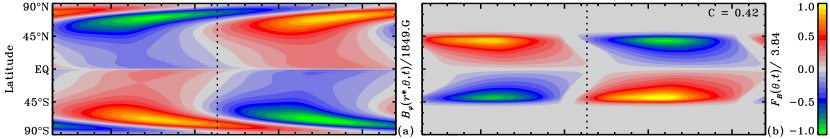
The large number of model parameters listed in Table 1 results from the very general forms adopted for many model ingredients, notably the meridional flow profile and emergence function. This gives the model great flexibility, in that it includes as a subset a number of published models. As an example and a form of validation exercise, we now reproduce a dynamo solution resembling that presented in MD2014.
Since MD2014’s model includes a full two-dimensional representation of the solar surface and an emergence algorithm similar to ours, direct contact is allowed between specific features of the two models despite significant differences in algorithmic implementation and numerical procedures. Their (single-cell) meridional circulation profile (described in Dikpati 2011) and magnetic diffusivity profile (described in Dikpati & Gilman 2007) may be closely approached by ours, through the parameter values listed in the first column of Table 1. Similarly, their emergence function is comparable to the one we describe in § II.4.2, with a latitudinal masking approximated by parameters and (a low-latitude cutoff conducive to the production of a solar-like butterfly diagram but hard to justify from the point of view of stability of thin flux tubes) and applied only to the component evaluated near depth . The magnetic masking includes a lower threshold of unspecified value and apparently no upper saturation threshold (parameter ). The detailed parametrization of individual emerging BMRs nonetheless differs significantly from ours, in a generally more deterministic manner. The latitude of emergence is directly associated with the location of peak toroidal field, as compare to the probabilistic approach we use. The tilt, separation, size and flux of the spot pair are mainly determined by the value of and the latitude of emergence, and so are deterministic rather than stochastic.
In order to minimize the differences associated with stochastic realizations of our emergence procedure, we limit this exercise to the input of observed emergences. Following Paper I, we use the comprehensive database of over 3000 BMRs gathered by Wang & Sheeley (1989) for cycle 21. By feeding these data into Equations (11a) and (11b), the D simulation is indirectly forced to run in a cycle-21-like mode. The remaining model parameters are set to mimic MD2014’s model (first column of Table 1). We obtain the two-cycles solution presented in Figure 1(a), for the synoptic evolution of at the base of the convection zone. This solutions resembles MD2014’s result in that it presents a strong mid-high-latitude poleward branch. Our low-latitude equatorial branch is however much weaker. Applying the appropriate latitudinal and magnetic mask from MD2014, we obtain the emergence function, or equivalently the probabilistic distribution of emergences, presented in Figure 1(b). This resembles the pattern of emergence produced in MD2014, with surface emergences strongly localized around latitude, with a hint of equatorward propagation (see their Figure 2a, keeping in mind that the slanted thick poleward streaks going from mid to high latitudes on this time–latitude plot reflect post-emergence surface flux transport, not emergence per se).
III.2. Numerical Optimization
We now seek to select model parameter values so as to obtain a solar-like dynamo solution. This defines a numerical optimization task which consists in optimizing the parameters listed in Table 1 to yield the closest possible fit to solar observations.
The first choice to be made is the goodness-of-fit measure to be used to drive such optimization. We opted to use a single fitness measure, namely the value of the linear correlation coefficient between the synoptic distribution of synthetic and observed emergences of BMRs. This presupposes that the magnetic flux tubes producing BMRs upon emergence through the photosphere rise radially through the convection zone, on a timescale very much shorter than the cycle period. Models based on the thin flux tube approximation support this idea, at least for the more strongly magnetized flux tube presumably producing the larger BMRs (see, e.g., Fan 2009, and references therein).
Next we must select a suitable observational dataset against which to optimize the model. As for the preceding validation exercise, we use Wang & Sheeley (1989)’s BMRs database for cycle 21. In order to minimize any influence of the initial condition (solar minimum-like dipolar configuration, as introduced in Paper I), we generate a sequence of eight replicates of the cycle 21 database (hereafter W218), by sequentially inverting the latitudes of emergence from one replication to the next, and use the output corresponding to the last two cycles to compute the correlation coefficient.
III.3. Genetic Algorithm (GA): PIKAIA
We perform the numerical optimization of using the GA-based optimizer PIKAIA 1.2111 http://www.hao.ucar.edu/modeling/pikaia/pikaia.php (March 2015) (Charbonneau & Knapp, 1995; Charbonneau, 2002). GAs allow for an efficient and adaptive exploration of the parameter space, and are thus quite robust at handling global optimization problems. As described in Paper I, they also allow for a quasi-Monte Carlo sampling of the parameter space about the current optimum solution, thus helping to construct error estimates on optimal parameter values. In the present context PIKAIA is operating in a 18-dimensional parameter space (viz. Table 1), with the fitness measure given by the correlation . Calculating the fitness of a single trial solution (18-parameter vector) implies running the SFT and FTD simulations in parallel, with appropriate coupling through the surface boundary condition, and finally evaluating . For our working spatial mesh and time stepping this requires about twenty minutes on a single-core modern CPU. For a typical optimization run of generations with trial solutions per generation, this adds up to core-days, but the fitness calculation being almost trivial to parallelize across the population, the wall-clock time can be brought down to a few days.
III.4. Choosing Parameter Ranges
PIKAIA is designed to carry out optimization in a bounded parameter space. The intervals explored for each parameter (second column of Table 1) are chosen to be physically meaningful and computationally stable. In particular, parameters , , and are restricted to the intervals found in Paper I to better reproduce surface synoptic magnetograms. Parameters , , and , however, are left free to vary in their original intervals despite the preceding calibration, to allow full exploration of the domain. Diffusivity values and and profile parameters , , and are given broad intervals but still within limits inferred by theoretical considerations and numerical experiments. Masking parameters are allowed to vary within ranges inferred from calculated stability diagrams, as described in § II.4.2.
III.5. Optimal Solution for Cycle 21
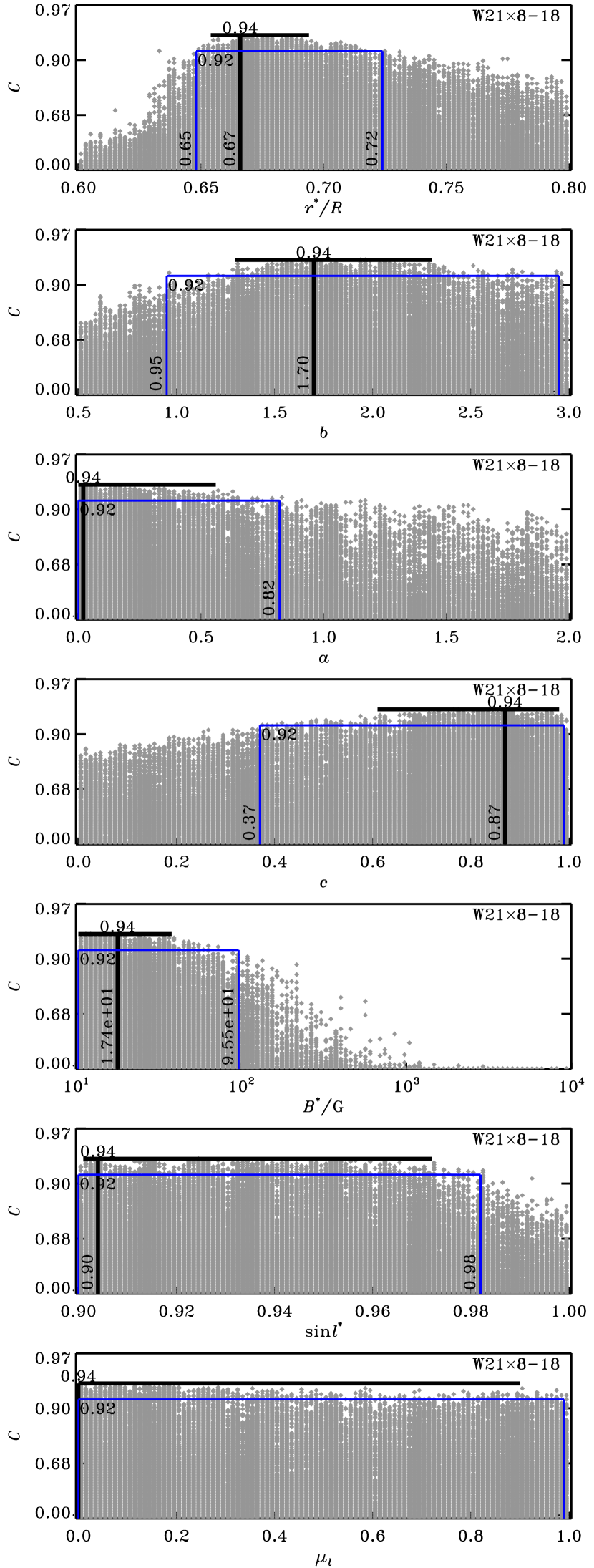
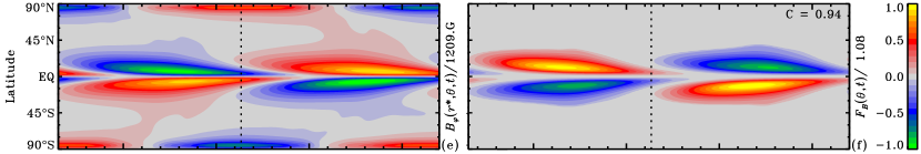
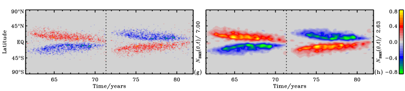
The first sequence of optimizations are run with all unconstrained parameters allowed to vary freely in the intervals listed in Table 1, hence called W218-18. We first analyse the model’s behavior relative to the parameters involved in the very definition of the emergence function (Equation (10)). Figure 2 illustrates the value of the goodness-of-fit as a function of emergence parameters , , , , , , and for a set of solutions obtained from four independent optimizations (different seed populations), generations each, trial solutions per generation. In all four optimizations, the fitness reaches the same optimal value . Such optimal solution, which parameters are listed in bold font in the rightmost column of Table 1, is presented in Figures 1(e) and 1(f). The fit between the emergence function (Figure 1(f)) and the smoothed butterfly diagram of cycle 21 emergences (Figure 1(h)) is good, with expected butterfly shapes and cycle overlaps.
However, it is clear from Figure 2 that considering only a single optimal solution is insufficient, optima being surrounded by a wide variety of sub-optimal but likely acceptable solutions, besides the clearly unacceptable ones. Also, all seven parameters presented are not equally constrained by the fitting procedure. By looking at all solutions standing above the level (thick black line), we get a first estimate of the relative restriction applied on each parameter. For instance, parameters , , and are fairly well constrained to a limited interval within the original boundaries, while parameters , , , and show wider regions of acceptable fit.
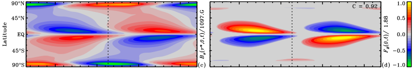
In order to build meaningful error estimates for each parameter, we must assess the physical limit of validity of the optimization criterion. Clearly, there must exist a value of above which solutions are physically acceptable, even if not strictly optimal. An example of such a solution, with , is presented in Figures 1(c) and 1(d). The butterfly shape in this solution is still clearly visible, though a second tail is starting to build towards the high latitudes. These differences are significant enough to declare such a solution inferior to the optimal one, but still at the limit of acceptability in terms of observed global features. The horizontal blue lines in Figure 2 delimit the solutions that are characterized by a criterion .
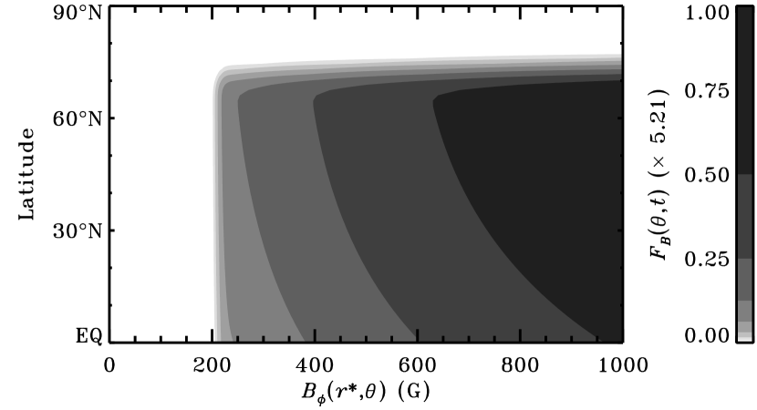
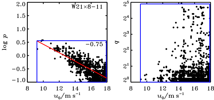
Before proceeding further into the parameters analysis, we now opt to get rid of the variability associated with the definition of the empirical emergence function (Equation (10)), and pick up definitive values, within the interval of acceptability, for the parameters involved. The inferred depth for the generation of flux instabilities is thus set near its optimal value , by averaging the magnetic field values between and . For simplicity, the relative contribution to of the poloidal field is set to zero (), while we round the optimal exponent of the toroidal contribution to . The lower threshold, above which this diffuse toroidal field is assumed to be able to generate instabilities, is set to its highest acceptable value, that is . The units of are in fact in the case to ensure coherence in Equation (10). This corresponds to a lower threshold of in , as illustrated in Figure 3. The emergence function remains proportional to , with , rather than saturating above . The highest latitude of emergence is fixed to (), in accordance with stability diagrams by Ferriz-Mas et al. (1994), and the equatorial intercept is set to , such that the latitudinal filter halves smoothly from down to the equator. The final emergence function (i.e. emergence probability) can now be mapped as a function of latitude and toroidal field amplitude, as shown in Figure 3, to form a synthetic “stability” diagram, which is the model’s equivalent to the stability diagrams presented in Ferriz-Mas et al. (1994, Figures 1 and 2).
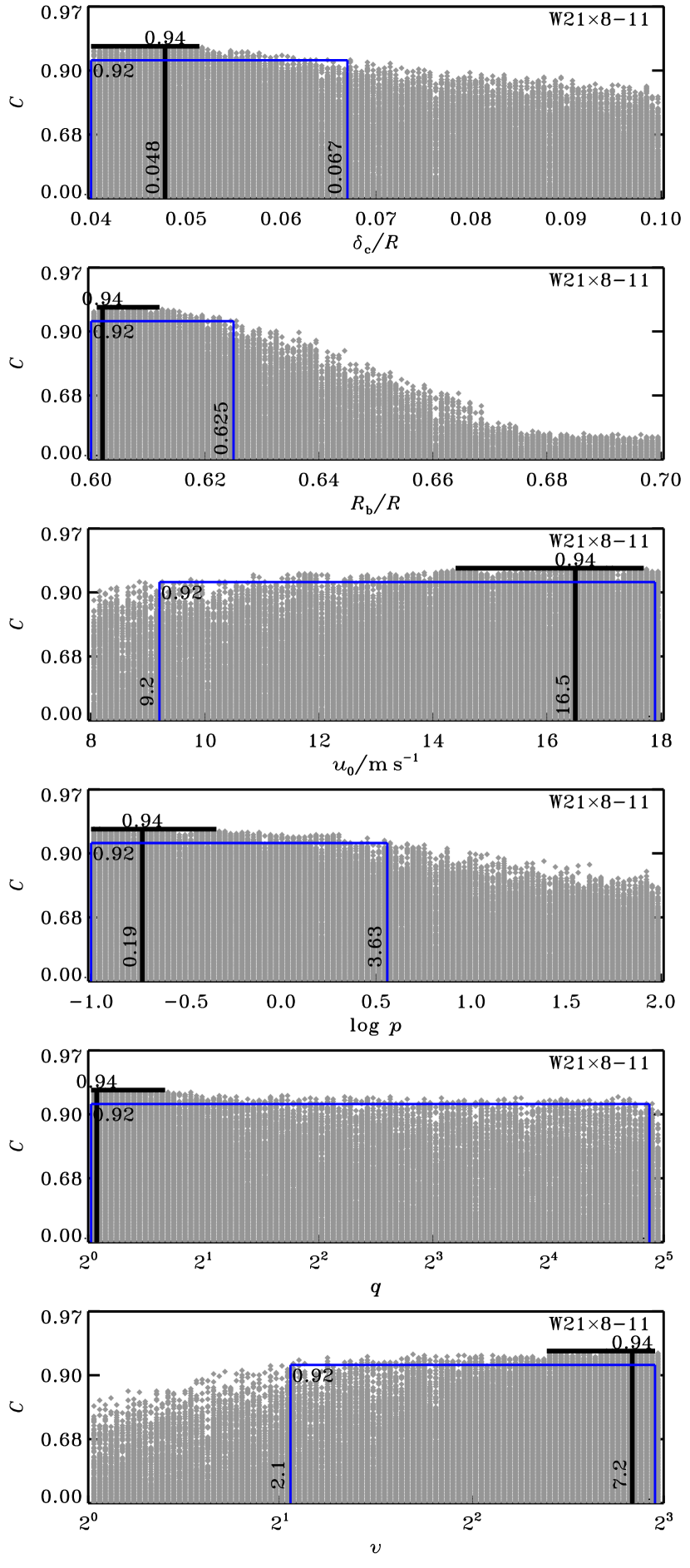
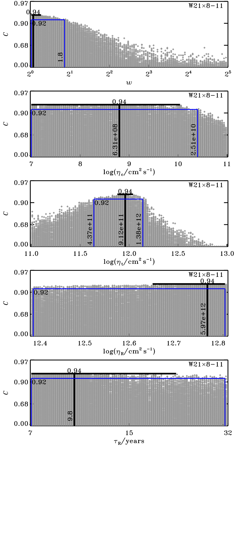
With the emergence function now fixed, we carry out a new series of four optimizations, hereafter called W218-11, with only the physical model parameters (, , , , , , , , , , and ) left to vary freely in their prescribed intervals. The corresponding solutions are presented in Figure 4 as a function of each parameter values. Again, the optimal fitness reaches , and all solutions characterized by a are considered acceptable. The corresponding interval for each parameter is used to define final error bars about the optimal values, as listed in the rightmost column of Table 1. As mentioned earlier, various combinations of parameters within these accepted intervals lead to acceptable solutions, but not all do, due to various correlations between some pairs of best-fit parameters (see also discussion in Paper I, § 3.5). Figure 5 depicts two of the strongest such correlations uncovered in our W218-11 set of solutions. The left panel shows a net linear (anti)correlation between the surface meridional flow speed and one of the parameters () setting the depth dependence of the meridional flow in the interior (viz. Equation 3a). This (anti)correlation has an unambiguous physical explanation: it leads to all solutions near the red line having an equatorward meridional flow speed equal to at , that is below the base of the convective envelope, beneath the layer where the emergence function is calculated. It is the speed of this return flow that sets the cycle period, and thus is strongly constrained by the sunspot butterfly diagram used to establish our goodness-of-fit measure. The right panel of Figure 5 shows another correlation between a pair of parameters, in the form of a somehow triangular constraint on parameter , which controls the polar end of the latitudinal dependence of the meridional flow, as a function of maximum flow speed (viz. Equation 3b). This correlation sets a lower limit on the surface flow speed at mid–high latitude, of the order of .
IV. A Solar-like Dynamo Solution
Now that the physical model and masking parameters have been properly calibrated to ensure that function reproduces the observed solar butterfly diagram of surface emergences, we may use it as the statistical emergence function it was meant to be, i.e. providing the missing surface source term with new emergences generated from deep seated toroidal flux (Equations (11a) and (11b)) and thus closing the loop for a self-consistent and autonomous D dynamo.
In all following cases, we use as initial condition the simulation state at the end of the previously calibrated W218 sequences. This ensures that the new simulations start up from a state representative of a solar activity minimum.
IV.1. Quasi-Linear Regime

The linearity in B of the FTD equations (7a) and (7b) and SFT equation (8) is expected to lead to either growing or decaying dynamo solutions. In the well-studied mean-field framework, this behavior is controlled by the “dynamo number”. Here it is the proportionality constant between and the absolute number of emerging BMRs per time step that plays the equivalent role. Since and in the definition of , and in Equation (10), the number of emerging BMRs is proportional to as long as the latter exceeds the lower threshold . However, the emergence process itself is inherently stochastic, so the dynamo growth rate can only be defined in a statistical sense, hence the “quasi-linear” labeling.
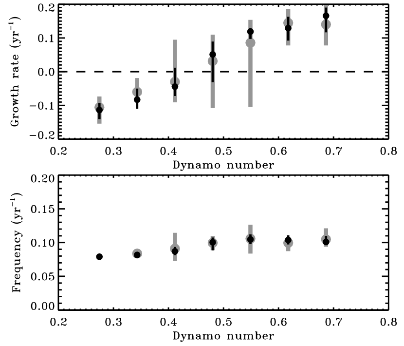
The top panel of Figure 6 depicts the temporal evolution of the total magnetic energy content inside the simulated Sun, for -cycles sample realizations of a D dynamo run in the quasi-linear regime at four different dynamo numbers . From these few samples, the transition between decaying (small ) and exponentially growing (large ) solutions seems sharp, but a more complete analysis reveals otherwise. The middle panel of Figure 6 shows how the growth rate of the magnetic energy can show a wide spread at a given value of . Error bars on the plot illustrate the intervals of growth rates obtained at each given , through ten different realizations of the statistical emergence procedure described earlier (cf. § II.4.2). We also performed a similar set of simulations in a reduced stochastic regime (shown in black on the plot). This reveals the strong global impact of stochasticity in the emergence process, particularly by the distributions in separations and tilts of emerging BMRs. The consequence is that a precise value for the critical dynamo number cannot be defined, with different realizations of the dynamo with resulting in dynamo solutions that can either grow or decay. The fact that this transition region lies significantly below the value required to reproduce the observed butterfly diagram for cycle 21 in the preceding section suggests that the dynamo should run in the supercritical regime, with some non-linear feedback regulating the mean cycle amplitude. This aspect will be discussed in the following subsection.
As another indicator of the model behavior, average cycle frequencies (periods) of the corresponding solutions, are also presented in the bottom panel of Figure 6, again with error bars showing the intervals of frequencies obtained for a given . Considering the difficulty of measuring cycle periods in quickly decaying oscillatory solutions (low ), no strong trend appears from this plot. This suggests how robust is the model at producing oscillations on a timescale, in spite of the strong variability associated with stochastic processes.
IV.2. Tilt-Quenching and Reference Dynamo Solutions
To overcome the problem of (quasi-)linearity, but without dealing explicitly with dynamical feedback, some ad hoc quenching may be added to the dynamo source terms. Motivated by the modeling of the buoyant rise of thin magnetic flux tubes by D’Silva & Choudhuri (1993) and Caligari et al. (1995) (for a review see Fan 2009, § 5.1.2, and references therein), we introduce a quenching of the BMR mean tilt as a function of the amplitude of the contributing underlying toroidal field , in order to mimic the resistance of magnetic tension in strongly magnetized flux tubes against the twisting imparted by the Coriolis force. Observationally the situation is less clear-cut (see § 6 in Pevtsov et al. (2014) for a recent review). Dasi-Espuig et al. (2010) and McClintock & Norton (2013) do find an influence of cycle amplitude on mean tilt angles, varying from cycle to cycle and from one solar hemisphere to another, but Stenflo & Kosovichev (2012) do not find a statistically significant relationship between tilt angles and flux of individual BMRs.
The quenched tilt is written
| (12) |
with some ajustable critical magnetic field amplitude. In the context of the present dynamo model, we find a tilt-quenching with , at dynamo number , to be adequate to generate stable dynamo solutions, comparable to solar amplitudes for the butterfly density plot and the monthly number of newly-emerged BMRs. The latter we refer to as a “pseudo-SSN”, since no consideration is given here to distinguishing groups vs individual emergences, or assigning them different weights, as is the case in the definition of the international SunSpot Number (SSN). For instance, observed cycle 21 peaks at a SSN of while the maximum monthly number of newly-emerged BMRs in Wang & Sheeley (1989)’s database is .
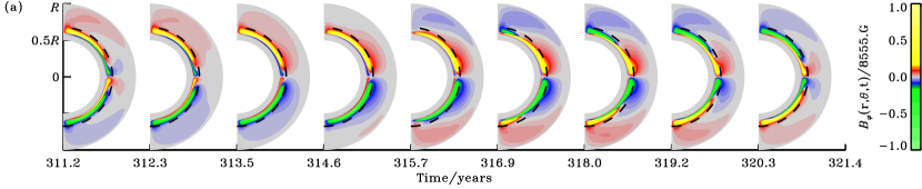
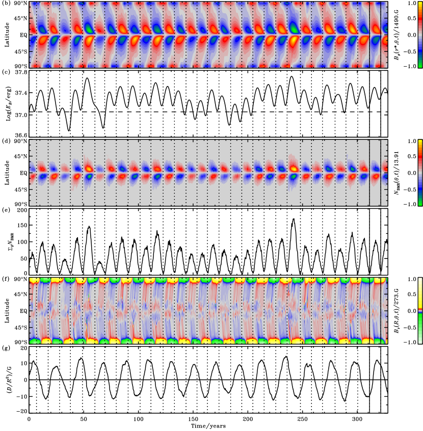
Figure 7(b)–(g) illustrate the evolution of the deep toroidal field, total magnetic energy, BMRs density, pseudo-SSN, surface radial field, and axial dipole moment for a sample dynamo solution run over more than years and roughly synthetic solar cycles. The temporal series exhibit solar-like behaviors in many aspects, in particular cycle periods varying between and years, cycle amplitude variations of a factor three to four in the pseudo-SSN, and long term variability such as some progressive increase of cycle amplitude after the occurence of a weak cycle or the triggering of small cycles after very strong ones. Some significant hemispheric asymmetries are also noticeable on the various plots, but polarity reversals remain sharply synchronized, indicating strong cross-hemispheric coupling. The oscillating surface axial dipole moment peaks at or near pseudo-SSN minimum, in agreement with observations. The phase relationship between the surface dipole and deep-seated toroidal field is also solar-like, with the dipole peaking at or shortly prior to pseudo-SSN minimum.
The overall amplitude of this dynamo solution is however slightly higher than that of the average solar cycle. The axial dipole moment (panel (g)) oscillates with an amplitude of as compared to for the Sun. The pseudo-SSN (panel (e)) peaks between and , which is slightly higher than average solar cycle amplitude ( for cycle 21). This corresponds to emergences per month near cycle maxima down to per month at cycle minima. The total number of BMRs to emerge during a cycle varies from for the smallest cycles to for the strongest ones, which is comparable, but again slightly higher in average, than the original BMRs extracted from Wang & Sheeley (1989)’s database for cycle 21. Due to the use of a constant log-normal distribution for BMR magnetic fluxes, total magnetic flux emerged during a cycle scales linearly with the number of BMRs. Finally, most presumably due to the use of a suboptimal profile for the surface meridional circulation leading to extra flux accumulation near the poles at activity minima, the peak amplitude of the radial surface field (panel (f)) builds up at an order of magnitude stronger than observed. At any rate, a dynamo number is more than sufficient to maintain stable dynamo solutions, with only the BL mechanism operating and without having to artificially enhance the emerging flux (see also Cameron & Schüssler 2015). The value of used here for the reference dynamo should even be brought down a little to better fit solar cycle observations.
Also shown in Figure 7(a) is a series of radius–latitude cuts of the toroidal field component, at nine different phases of a synthetic sunspot cycle. The toroidal field reverses amplitude after , which is slightly shorter than the average observed sunspot cycle. The peak toroidal field amplitude near is reached at mid-cycle, near maximum sunspot activity. Below the tachocline, the magnetic field from three to four successive cycles piles up to thinner and thinner layers as it reaches the depth . This is precisely what is to be expected from the average diffusivity used at , which corresponds to a diffusive time-scale of years. Below , the magnetic diffusivity of , leads to a diffusive time-scale years. Therefore, while the meridional circulation acts on a time-scale commensurate with the sunspot cycle period, the deep diffusive processes act on much longer timescales. The remnants from old cycles appear to be able to feed back into the dynamo system and induce some long term memory in cycle amplitude.

Figure 8 shows some long term interrelations between cycle properties, extracted from the preceding dynamo solution. Panel (c) in the figure shows the strong linear correlation () obtained between amplitude (maximum pseudo-SSN) of a cycle () and maximum axial dipole moment at the end of the preceding cycle (). This behavior is to be expected from the quasi-linear transport and shearing of the poloidal magnetic field accumulated at cycle minimum into a deep toroidal component peaking at cycle maximum and generating a proportional number of surface emergences. As shown in panel (d) of the figure, the reverse correlation is not true, however, as the stochastic properties of emerged BMRs during a given cycle destroy the otherwise expected correlation between pseudo-SSN and axial dipole amplitude at the end of the same cycle (). Also, even if long term magnetic memory does exist in the interior, the poor correlations obtained between amplitude of cycle and axial dipole moment at the end of cycles (panel (b)) and cycles (panel (a)) indicate that it is erased by the stochasticity of flux emergence. Despite these stochastic sources of fluctuations, hemispheric cycle amplitudes remain strongly correlated, as shown in Figure 8(f). All the preceding results are in good agreement with observed solar cycle characteristics (see, e.g., Muñoz-Jaramillo et al. 2013, Figure 5).
As also shown in panel (e) of Figure 8, cycle amplitude and period are essentially uncorrelated. This differs from the behavior observed in the Sun, where a significant anticorrelation is inferred between these two cycle measures. Some additional dynamical feedback would likely be required to reproduce such behavior.
IV.3. Long Term Variability
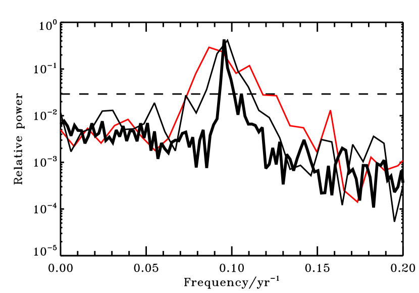
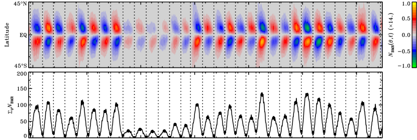
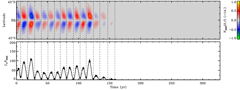
Figure 9 shows the Fourier transforms of the pseudo-SSN time series, for a sample 32-cycles tilt-quenched D dynamo simulation similar to the reference solution of Figure 7, along with the average spectra constructed from three statistically independent realizations of a 96-cycles simulation. The relatively poor sampling of the 32-cycles simulation shows spectral features similar to those of the 23-cycles solar SSN spectrum (also shown in the figure), in that it presents a broad peak between periods of to ( to for the SSN) as well as low amplitude ( of peak power) structures at other frequencies. However, these secondary features occur at different frequencies for the SSN and for different realizations of the pseudo-SSN, and so do not represent physically robust signals. Indeed, the averaging of three 96-cycles spectra (equivalent to cycles in total) reveals no hint of low-frequency signature above of peak power, of the type one would associate with the so-called Gleissberg or Suess cycles detected in temporally-extended records of solar activity. The cycle period is also much more robust, at . These results indicate that despite the strong variability in cycle amplitude characterizing the simulations, the period is very stable, even more so than in the real Sun.
Figure 10 shows two sets of synthetic butterfly diagrams and associated pseudo-SSN time series, obtained for the same parameter values as the solution of Figure 7 but using distinct stochastic realizations for the fluctuating properties of the synthetic BMRs. The top solution generally resembles panels (d) and (e) of Figure 7 in its overall amplitude fluctuation pattern, but now also shows an episode of strongly reduced cycle amplitude, persisting here for four cycles () and reminiscent of the 1796–1825 Dalton minimum of the sunspot record. Entry into this low amplitude episode is sudden, the preceding few cycles being of average amplitude or higher. Recovery is however more gradual, with a few cycles required for the cycle to build back up to its pre-event average amplitude.
The solution plotted on the two bottom panels of Figure 10 shows yet another interesting behavior: a complete halt of the cyclic dynamo, here at , following a sequence of unfavorably positioned and/or tilted large BMRs, leading to a much reduced dipole moment building up in the descending phase of the cycle peaking at . Because of the lower cutoff built into our emergence function (viz. Equation (10) herein), once the toroidal magnetic field falls below this threshold, BMRs are no longer produced, so that the existing dipole then undergoes simple resistive decay, followed by resistive decay of the toroidal component, as per Cowling’s theorem. A distinct inductive mechanism able to operate at low mean-field strengths, such as the alpha-effect of classic mean-field electrodynamics, would be needed here to restart the dynamo cycle (see, e.g., Passos et al. 2014). Ongoing numerical experiments along these lines suggest that this would be a feasible path towards the generation of solar-like Grand Minima of activity.
In a set of realizations similar to the one displayed in Figure 7 and the two in Figure 10, seven shut off before reaching the th cycle, and 15 before reaching the th cycle. The probability of a dynamo to remain active after a certain number of cycles thus decreases with time in a manner that appears consistent with a stationary memoryless random process, as would be expected from the stochastic nature of the properties of emerging BMRs built into the model. A detailed, quantitative investigation of these matters, currently underways, will be the focus of a subsequent paper in this series.
V. Discussion
The dynamo solutions presented above result from the use of a model calibrated to cycle 21 emergence data through an optimization process operating on a specific goodness-of-fit measure and in a bounded search space. These bounds were set (loosely) on observational and/or physical grounds, but obviously pose a restriction on the range of solutions accessible to the optimization. Could we do better than the optimal solution listed in Table 1 ? We have carried out a number of alternate optimization runs in order to answer this question, as described in what follows.
An 18-parameter optimization similar to that described in § III.5 but using much broader ranges of parameter does manage to return a best-fit solution with , significantly better than the original 18-parameter best-fit solution, which has . This nominally superior fit, however, is achieved through a low-latitude cutoff for the emergence function, down to , which is clearly incompatible with stability diagrams for thin toroidal flux ropes.
We also carried out optimization runs in which the parameters defining the latitudinal dependence of the meridional flow (via Equations (3a)—(3b)) are constrained to a narrower range of acceptable values, corresponding to the best-fit surface flux transport solution obtained in Paper I by fitting actual synoptic magnetograms, rather than just the spatiotemporal distributions of BMR emergences. The best-fit solution from such an optimization reaches only , which is much less satisfactory than the best-fit solution. More worrisome is the fact that the surface meridional flow for the best-fit solution and error bars of Table 1, plotted in Figure 11 (dark gray band), provides a rather poor fit to the Doppler observations of Ulrich (2010), which lie mostly outside the range of acceptable solutions from the optimization run. The best-fit profile of Paper I did much better in this respect (reproduced herein as the pale gray band in Figure 11).
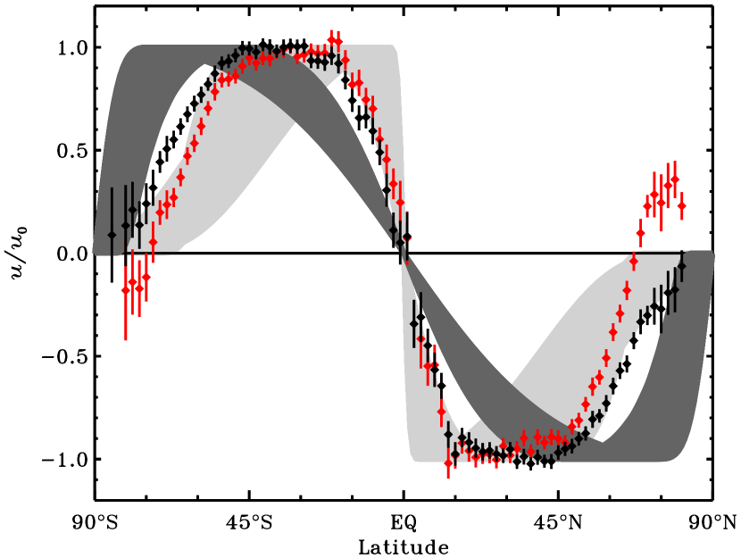
This suggests some incompatibility between the optimization of the SFT model relative to surface magnetograms and the optimization of the coupled SFT–FTD model relative to the shape of the sunspot butterfly diagram. The W218-11 optimal solution of § III.5 still lies within the surface-optimized ranges for the maximum meridional flow amplitude , the surface diffusivity , and the exponential decay time obtained in paper I, while the parameters , and (see Equation (3b)), setting the latitudinal dependence of the stream function, do not. Interestingly, despite significant variations in latitudinal profiles, all acceptable solutions ) have a peak equatorward meridional flow speed of near the base of the circulation cell; this is consistent with the deep meridional flow setting the cycle period in these dynamo solutions, which leads to a very tight constraint when fitting the butterfly diagram.
The analytic form adopted here for the meridional flow stream function is of course extremely simple: steady and separable in and , which enforces the same latitudinal dependence at all depths, and defining a single flow cell per meridional quadrant. What our butterfly diagram-based goodness-of-fit measure thus constrains is primarily the flow at the base of the convection zone. The misfit with the results from purely surface optimization suggests that the internal flow is more complex than the single-cell profile used here. Indeed, the recent helioseismic inversions of Zhao et al. (2013) and Schad et al. (2013) suggest multiple cells in radius, which is known to have a large impact on the operation of flux transport dynamos (e.g., Jouve & Brun 2007). The dynamo modeling work of Hazra et al. (2014a) indicates, however, that provided additional transport processes such as turbulent diffusion and/or pumping can couple the surface and base of the convection zone, solar-like butterfly diagrams can be produced as long as an equatorward flow is present at or immediately beneath the base of the convection zone (see also Jiang et al. 2013).
Another physical inconsistency of the W218-11 optimal solution is the meridional flow’s deep penetration below the base of the convection zone. This is known to be conducive to the production of solar-like butterfly diagrams (e.g., Nandy & Choudhuri 2002), but unlikely on dynamical grounds (Gilman & Miesch, 2004), and delicate to reconcile with observed solar light element abundances (Charbonneau, 2007). Finally, both observations (Ulrich, 2010) and numerical simulations (Passos et al., 2012) suggest that the meridional flow may undergo systematic temporal variations in the course of the cycle, presumably driven by the cycling magnetic field. Such effects are a priori excluded from the meridional flow parametrization used here.
All these incompatibilities and inconsistencies most likely reflect, at least in part, the specific choices made for the parametrization of the meridional flow profile. An interesting possibility would be to use our GA-based fitting technique to invert a spatially-resolved discretization of the internal meridional flow from the sunspot butterfly diagram. Such a method, dubbed genetic forward modeling, has already been used successfully to infer the rotational profile of the deep solar core from low- rotational frequency splittings (see Charbonneau et al. 1998).
Genetic forward modeling could also be used to invert stability diagrams for the emergence of BMRs. Our best-fit emergence function has in Equation (10), implying that the emergence probability is primarily set by the strength of the toroidal magnetic component, in agreement with the idea that sunspots form from axisymmetric toroidal magnetic flux ropes located at or near the base of the convection zone. However, our eruption threshold of is rather low, even if some level of amplification is expected in forming a compact flux rope from a diffuse magnetic field. There is clearly room for improvement in this model component.
VI. Conclusions
In this paper we have described a new solar cycle model based on the Babcock–Leighton mechanism of poloidal field regeneration through the surface decay of active regions. This new model is based on the coupling of a conventional latitude–longitude simulation of surface magnetic flux evolution (as described in Paper I), coupled to an equally conventional axisymmetric kinematic flux transport dynamo model defined in a meridional plane (closely following Charbonneau et al. 2005). The novelty lies in the coupling between these to model components: the surface flux evolution simulation provides the source term of the internal dynamo through the surface boundary condition; while the internal dynamo provides the magnetic flux emergence, in the form of pseudo-sunspot bipolar pairs, that act as a source in the surface magnetic flux simulation. The properties of these synthetic bipolar pairs —flux distribution, component separation, tilt angles, etc— are tailored to reflect observed statistical properties of real sunspots and active regions, as documented in Paper I (Appendix).
The other key aspect of the coupling is the emergence function, which controls the probability of bipole emergence as a function of the spatiotemporal distribution of the deep-seated magnetic field produced by the dynamo component of the coupled model. The emergence probability is assumed to scale linearly with this emergence function, with the proportionality constant acting as the dynamo number for the full coupled model.
The coupled model involves a number of parameters and functionals that cannot be set from first principle, and thus must be optimized to provide the best possible fit to solar observations. We opted to carry out this optimization task through a genetic algorithm-based maximization of the fit between the spatiotemporal distribution of sunspot emergences (butterfly diagram) as produced by the model, and the cycle 21 emergence data of Wang & Sheeley (1989). This scheme returns not only a globally optimal solution, but also Monte Carlo-like error estimates on best-fit parameters values.
The magnetic cycles generated by this dynamo model are intrinsically non-steady, due primarily to the large statistical scatter about the mean East–West tilt pattern of BMRs (as embodied in Joy’s Law). This is expected, since the axial dipole component of the bipolar pair is determined by this tilt. As a consequence, a critical dynamo number can only be defined in a statistical sense.
A quenching parametrization of the mean tilt angle based on the strength of the internal magnetic field readily stabilizes the mean cycle amplitude, but large fluctuations about this mean nonetheless persist. Such a quenching is consistent with the modeling of the buoyant rise of thin magnetic flux tubes (see Fan 2009, § 5.1.2, and references therein), and, at the relatively mild level taking place in our dynamo model, does not conflict with extant observational analyses (see Pevtsov et al. 2014). One consequence of tilt quenching is that a very high amplitude cycle tend to be followed by a lower-than-average cycle. This alternation would tend to amplify over time were it not for the stabilizing effect of the linear sink term used in Equation (8) with . Very low amplitude cycles can also be produced by unfavorable emergence patterns, which then lead to persistently low amplitudes in subsequent cycles, with slow recovery to normal amplitude values.
Even though the amplitude of successive simulated cycles are strongly affected by the specific stochastic realization of flux, separation and tilts in the course of a given cycle, even in the linear regime the cycle period is largely insensitive to the value of the dynamo number. The magnetic cycle is also characterized by good hemispheric coupling, in terms of both hemispheric cycle amplitude and timing of hemispheric minima/maxima.
As a descriptive representation of the observed solar cycle, the model reproduces a number of well-known features. The dipole peaks at or slightly before the time of pseudo-sunspot cycle minimum, and its amplitude shows no correlation with the maximum pseudo-sunspot number of the ending cycle. This is a direct consequence of the strong stochasticity introduced by the realization of tilt patterns throughout the cycle, which is the primary source of cycle amplitude fluctuations. However, the model reproduces the observed positive correlation between dipole strength at cycle minimum and the amplitude of the subsequent pseudo-sunspot cycle. This indicates that, as in the real Sun, the dipole moment generated in the model is a good precursor of cycle amplitude.
Room for improvement certainly remains. The model fails to reproduce the observed moderate anticorrelation between cycle amplitude and duration, yielding instead a very weak positive correlation between these two quantities. While a few extant kinematic flux transport dynamo models do better in this respect (e.g., Karak & Choudhuri 2011), another possibility is that the origin of this pattern is to be found in dynamical effects, namely the magnetic backreaction on large-scale flows. The recent analyses of Passos et al. (2012) suggest that an increase in the speed of the deep equatorward meridional flow may indeed be driven by a higher-than-average large-scale magnetic field, which in advection-dominated flux transport dynamos would be expected to lead to a proportional reduction in cycle period (see, e.g., Dikpati & Charbonneau 1999).
The long timescale behavior of the simulated cycles also shows some interesting features, some solar-like and others less so. The model produces a very stable cycle period of years, but no well-defined low-frequency spectral peaks that could be associated with Gleissberg-like long periodicities. The model does produce occasional Dalton-minimum-like periods of successive low amplitude cycles, and can also spontaneously shut down the cycle and enter a non-cycling grand-minima-like state, through an unfavorable stochastic pattern of bipolar pseudo-sunspot emergences in the course of a cycle. This is a relatively common occurrence for a simulation using the best-fit parameter values obtained in § III: more than one half of simulations initialized with distinct random seeds were found to undergo shutdown at some point during a 100-cycle long time span.
In subsequent papers in this series we will investigate cycle fluctuation patterns in greater detail, and quantify the occurrence statistics of Dalton-like minima. The few such events found so far in our extant simulation runs suggest that entry into these failed minima is rapid, from one cycle to the next, while recovery to average cycle amplitudes is more gradual. We also plan to add a weak turbulent alpha-effect in the convective envelope portion of the domain, and investigate whether this can pull the model out of a shutdown state, as existing simulations have already suggested (e.g., Ossendrijver 2000; Karak & Choudhuri 2013; Hazra et al. 2014b).
Because it includes an explicit, spatially-resolved representation of the solar “surface”, the D solar cycle model presented here is ideally suited for providing synthetic data for coronal magnetic field reconstructions, as well as for assimilation of magnetographic data towards solar cycle forecasting. The results presented in this paper indicate that an accurate determination of the tilt angles of individual emerging bipolar sunspot pairs will be a critical element of such latter endeavor.
- AR
- active region
- BL
- Babcock–Leighton
- BMR
- bipolar magnetic region
- FTD
- flux transport dynamo
- GA
- Genetic Algorithm
- MHD
- magnetohydrodynamics
- probability distribution function
- RMS
- root-mean-square
- SFT
- surface flux transport
- WS
- Wang and Sheeley
References
- Babcock (1959) Babcock, H. D. 1959, ApJ, 130, 364
- Babcock (1961) Babcock, H. W. 1961, ApJ, 133, 572
- Babcock & Babcock (1955) Babcock, H. W., & Babcock, H. D. 1955, ApJ, 121, 349
- Baumann et al. (2006) Baumann, I., Schmitt, D., & Schüssler, M. 2006, A&A, 446, 307
- Baumann et al. (2004) Baumann, I., Schmitt, D., Schüssler, M., & Solanki, S. K. 2004, A&A, 426, 1075
- Bogdan et al. (1988) Bogdan, T. J., Gilman, P. A., Lerche, I., & Howard, R. 1988, ApJ, 327, 451
- Burnett (1987) Burnett, D. S. 1987, Finite Element Analysis: From Concepts to Applications (Reading, Massachusetts: Addison-Wesley Pub. Co.)
- Caligari et al. (1995) Caligari, P., Moreno-Insertis, F., & Schussler, M. 1995, ApJ, 441, 886
- Cameron & Schüssler (2015) Cameron, R., & Schüssler, M. 2015, Science, 347, 1333
- Charbonneau (2002) Charbonneau, P. 2002, NCAR Tech. Note, NCAR/TN-451+STR (Boulder: National Center for Atmospheric Research), 1
- Charbonneau (2007) Charbonneau, P. 2007, Advances in Space Research, 39, 1661
- Charbonneau (2010) —. 2010, Living Reviews in Solar Physics, 7, 3
- Charbonneau (2014) —. 2014, ARA&A, 52, 251
- Charbonneau et al. (1999) Charbonneau, P., Christensen-Dalsgaard, J., Henning, R., et al. 1999, ApJ, 527, 445
- Charbonneau & Knapp (1995) Charbonneau, P., & Knapp, B. 1995, NCAR Tech. Note, NCAR/TN-418+IA (Boulder: National Center for Atmospheric Research), 1
- Charbonneau et al. (2005) Charbonneau, P., St-Jean, C., & Zacharias, P. 2005, ApJ, 619, 613
- Charbonneau et al. (1998) Charbonneau, P., Tomczyk, S., Schou, J., & Thompson, M. J. 1998, ApJ, 496, 1015
- Choudhuri et al. (2007) Choudhuri, A. R., Chatterjee, P., & Jiang, J. 2007, Physical Review Letters, 98, 131103
- Choudhuri et al. (1995) Choudhuri, A. R., Schüssler, M., & Dikpati, M. 1995, A&A, 303, L29+
- Dasi-Espuig et al. (2010) Dasi-Espuig, M., Solanki, S. K., Krivova, N. A., Cameron, R., & Peñuela, T. 2010, A&A, 518, A7
- Dikpati (2011) Dikpati, M. 2011, ApJ, 733, 90
- Dikpati & Charbonneau (1999) Dikpati, M., & Charbonneau, P. 1999, ApJ, 518, 508
- Dikpati et al. (2006) Dikpati, M., de Toma, G., & Gilman, P. A. 2006, Geophys. Res. Lett., 33, 5102
- Dikpati & Gilman (2001) Dikpati, M., & Gilman, P. A. 2001, ApJ, 559, 428
- Dikpati & Gilman (2007) —. 2007, Sol. Phys., 241, 1
- D’Silva & Choudhuri (1993) D’Silva, S., & Choudhuri, A. R. 1993, A&A, 272, 621
- Durney (1995) Durney, B. R. 1995, Sol. Phys., 160, 213
- Fan (2009) Fan, Y. 2009, Living Reviews in Solar Physics, 6, 4
- Fan & Fang (2014) Fan, Y., & Fang, F. 2014, ApJ, 789, 35
- Ferriz-Mas et al. (1994) Ferriz-Mas, A., Schmitt, D., & Schuessler, M. 1994, A&A, 289, 949
- Gilman & Miesch (2004) Gilman, P. A., & Miesch, M. S. 2004, ApJ, 611, 568
- Hale et al. (1919) Hale, G. E., Ellerman, F., Nicholson, S. B., & Joy, A. H. 1919, ApJ, 49, 153
- Hazra et al. (2014a) Hazra, G., Karak, B. B., & Choudhuri, A. R. 2014a, ApJ, 782, 93
- Hazra et al. (2014b) Hazra, S., Passos, D., & Nandy, D. 2014b, ApJ, 789, 5
- Howard (1991) Howard, R. F. 1991, Sol. Phys., 136, 251
- Jiang et al. (2013) Jiang, J., Cameron, R. H., Schmitt, D., & Işık, E. 2013, A&A, 553, A128
- Jouve & Brun (2007) Jouve, L., & Brun, A. S. 2007, A&A, 474, 239
- Karak & Choudhuri (2011) Karak, B. B., & Choudhuri, A. R. 2011, MNRAS, 410, 1503
- Karak & Choudhuri (2013) —. 2013, Research in Astronomy and Astrophysics, 13, 1339
- Karak et al. (2014) Karak, B. B., Jiang, J., Miesch, M. S., Charbonneau, P., & Choudhuri, A. R. 2014, Space Sci. Rev., 186, 561
- Leighton (1964) Leighton, R. B. 1964, ApJ, 140, 1547
- Lemerle et al. (2015) Lemerle, A., Charbonneau, P., & Carignan-Dugas, A. 2015, ApJ, 810, 78
- McClintock & Norton (2013) McClintock, B. H., & Norton, A. A. 2013, Sol. Phys., 287, 215
- Miesch & Dikpati (2014) Miesch, M. S., & Dikpati, M. 2014, ApJ, 785, L8
- Miesch & Teweldebirhan (2015) Miesch, M. S., & Teweldebirhan, K. 2015, ArXiv e-prints, arXiv:1511.03613
- Muñoz-Jaramillo et al. (2013) Muñoz-Jaramillo, A., Dasi-Espuig, M., Balmaceda, L. A., & DeLuca, E. E. 2013, ApJ, 767, L25
- Muñoz-Jaramillo et al. (2010) Muñoz-Jaramillo, A., Nandy, D., Martens, P. C. H., & Yeates, A. R. 2010, ApJ, 720, L20
- Nandy & Choudhuri (2001) Nandy, D., & Choudhuri, A. R. 2001, ApJ, 551, 576
- Nandy & Choudhuri (2002) —. 2002, Science, 296, 1671
- Nelson et al. (2013) Nelson, N. J., Brown, B. P., Brun, A. S., Miesch, M. S., & Toomre, J. 2013, ApJ, 762, 73
- Nelson et al. (2014) Nelson, N. J., Brown, B. P., Sacha Brun, A., Miesch, M. S., & Toomre, J. 2014, Sol. Phys., 289, 441
- Ossendrijver (2000) Ossendrijver, M. A. J. H. 2000, A&A, 359, 1205
- Parker (1955) Parker, E. N. 1955, ApJ, 122, 293
- Passos & Charbonneau (2014) Passos, D., & Charbonneau, P. 2014, A&A, 568, A113
- Passos et al. (2012) Passos, D., Charbonneau, P., & Beaudoin, P. 2012, Sol. Phys., 279, 1
- Passos et al. (2014) Passos, D., Nandy, D., Hazra, S., & Lopes, I. 2014, A&A, 563, A18
- Pevtsov et al. (2014) Pevtsov, A. A., Berger, M. A., Nindos, A., Norton, A. A., & van Driel-Gesztelyi, L. 2014, Space Sci. Rev., 186, 285
- Schad et al. (2013) Schad, A., Timmer, J., & Roth, M. 2013, ApJ, 778, L38
- Schmitt (1987) Schmitt, D. 1987, A&A, 174, 281
- Schrijver et al. (2002) Schrijver, C. J., De Rosa, M. L., & Title, A. M. 2002, ApJ, 577, 1006
- Schüssler et al. (1994) Schüssler, M., Caligari, P., Ferriz-Mas, A., & Moreno-Insertis, F. 1994, A&A, 281, L69
- Snodgrass (1983) Snodgrass, H. B. 1983, ApJ, 270, 288
- Stenflo & Kosovichev (2012) Stenflo, J. O., & Kosovichev, A. G. 2012, ApJ, 745, 129
- Ulrich (2010) Ulrich, R. K. 2010, ApJ, 725, 658
- van Ballegooijen & Choudhuri (1988) van Ballegooijen, A. A., & Choudhuri, A. R. 1988, ApJ, 333, 965
- Wang et al. (2002a) Wang, Y.-M., Lean, J., & Sheeley, Jr., N. R. 2002a, ApJ, 577, L53
- Wang et al. (1989) Wang, Y.-M., Nash, A. G., & Sheeley, Jr., N. R. 1989, Science, 245, 712
- Wang & Sheeley (1989) Wang, Y.-M., & Sheeley, Jr., N. R. 1989, Sol. Phys., 124, 81
- Wang & Sheeley (1991) —. 1991, ApJ, 375, 761
- Wang et al. (2002b) Wang, Y.-M., Sheeley, Jr., N. R., & Lean, J. 2002b, ApJ, 580, 1188
- Weber et al. (2011) Weber, M. A., Fan, Y., & Miesch, M. S. 2011, ApJ, 741, 11
- Yeates & Muñoz-Jaramillo (2013) Yeates, A. R., & Muñoz-Jaramillo, A. 2013, MNRAS, 436, 3366
- Zhao et al. (2013) Zhao, J., Bogart, R. S., Kosovichev, A. G., Duvall, Jr., T. L., & Hartlep, T. 2013, ApJ, 774, L29