Effects of the scatter in sunspot group tilt angles on the large-scale magnetic field at the solar surface

Abstract

The tilt angles of sunspot groups represent the poloidal field source in Babcock-Leighton-type models of the solar dynamo and are crucial for the build-up and reversals of the polar fields in Surface Flux Transport (SFT) simulations. The evolution of the polar field is a consequence of Hale’s polarity rules, together with the tilt angle distribution which has a systematic component (Joy’s law) and a random component (tilt-angle scatter). We determine the scatter using the observed tilt angle data and study the effects of this scatter on the evolution of the solar surface field using SFT simulations with flux input based upon the recorded sunspot groups. The tilt angle scatter is described in our simulations by a random component according to the observed distributions for different ranges of sunspot group size (total umbral area). By performing simulations with a number of different realizations of the scatter we study the effect of the tilt angle scatter on the global magnetic field, especially on the evolution of the axial dipole moment. The average axial dipole moment at the end of cycle 17 (a medium-amplitude cycle) from our simulations was 2.73G. The tilt angle scatter leads to an uncertainty of 0.78 G (standard deviation). We also considered cycle 14 (a weak cycle) and cycle 19 (a strong cycle) and show that the standard deviation of the axial dipole moment is similar for all three cycles. The uncertainty mainly results from the big sunspot groups which emerge near the equator. In the framework of Babcock-Leighton dynamo models, the tilt angle scatter therefore constitutes a significant random factor in the cycle-to-cycle amplitude variability, which strongly limits the predictability of solar activity.

1 Introduction

Hale et al. (1919) were the first to notice the systematic tilt of the line joining the two polarities of a sunspot group with respect to the East-West direction. The increase of the average tilt angle with heliographic latitude later became known as ‘Joy’s Law’. Detailed studies (e.g., Howard, 1991a; Sivaraman et al., 1999, 2007; Dasi-Espuig et al., 2010; McClintock & Norton, 2013) used the records of sunspots based on white-light photographs from the observatories at Mount Wilson in the interval 1917–1985 (Howard et al., 1984) and at Kodaikanal in the interval 1906–1987 (Ravindra et al., 2013). Since these data do not provide magnetic polarity information, the identification of the leading (westward) and following (eastward) parts of sunspot groups had to be based on visual inspection of the group morphology. Studies based on the magnetograms (Wang & Sheeley, 1989; Howard, 1991b, c; Tian et al., 1999, 2003; Stenflo & Kosovichev, 2012; Li & Ulrich, 2012) more accurately define the leading and following parts on the basis of the magnetic polarities, but they are less complete in their coverage of sunspot groups (or bipolar magnetic regions) and cover at most only 3 cycles. Regardless of the type of data, all studies based on a large sample of sunspot groups or bipolar regions confirm Joy’s law, i.e., a systematic increase of the average tilt angle away from the equator. They also consistently find a large scatter of the individual tilt angles about the mean.

A possible physical explanation of Joy’s law and the scatter of the tilt angles is suggested by simulations of rising magnetic flux tubes in the rotating solar convective envelope (D’Silva & Choudhuri, 1993; Fan et al., 1993; Caligari et al., 1995; Fisher et al., 1995; Fan, 2009; Weber et al., 2013). In these simulations, the Coriolis force acting on the expanding flows along a buoyantly rising flux loop leads to a latitudinal tilt of the loop that is consistent with Joy’s law. Weber et al. (2013) show that the mean tilt angles (Joy’s law) depend on the strength of the magnetic field in the flux tubes but are not significantly dependent on the total flux of the tube. The effects of the turbulent convective flows on a rising flux tube were studied by Fisher et al. (1995), Longcope & Fisher (1996) and, more recently, by Weber et al. (2011, 2013). The simulations show that, for flux tubes with field strengths above 30kG, convective flows introduce more scatter into tubes with less flux, because such tubes are more susceptible to deformation by convective flows. The inverse correlation between the scatter in the tilt angle and the flux of active regions are consistent with observations (e.g. the observational results in Stenflo & Kosovichev, 2012, who suggest a different intepretation). Other possible physical mechanisms for both Joy’s law and the scatter in the tilt angles remain to be explored. In this paper we restrict our attention to measuring the scatter and determining its consequences on the evolution of the large-scale magnetic field of the Sun.

The tilt angles of sunspot groups and, more generally, bipolar magnetic regions have a considerable effect on the evolution of the large-scale distribution of magnetic flux on the solar surface. The tilt corresponds to a latitudinal offset of the two polarities of a bipolar region. As a result of Hale’s polarity laws, this offset is consistent across both hemispheres: during one half of a 22-year magnetic cycle (during which, say, the North pole in the beginning has negative polarity), the positive polarity of the emerging bipolar regions is displaced northward from the negative polarity (on average) in both hemispheres. The transport of the magnetic flux by surface flows then leads to reversals of axial dipole moment and polar fields. In the next magnetic half-cycle, all polarities are reversed. In the framework of Babcock-Leighton dynamos, it is through this process based upon the tilt angle that toroidal field is converted to poloidal field and the dynamo loop is closed (see review by Charbonneau, 2010).

Given its fundamental importance for the evolution of the large-scale magnetic field and its role in Babcock-Leighton dynamo models, systematic and random variations of the tilt angles are important for a quantitative understanding of these processes (Jiang et al., 2013a). Using the Mount Wilson and Kodaikanal tilt angle data, Dasi-Espuig et al. (2010) found an anti-correlation between the mean tilt angle (normalized by emergence latitude) of a given cycle and the strength of that cycle (see also McClintock & Norton, 2013). Cameron et al. (2010) included this observed cycle-to-cycle variation in a surface flux transport simulation, which reproduced the empirically derived time evolution of the solar open magnetic flux and the reversal times of the polar fields between 1913 and 1986.

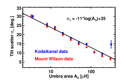
Figure 2: Standard deviations of the observed tilt angle distributions binned in logarithmic umbral area. Kodaikanal data are indicated in blue, Mount Wilson in red. The solid curve represents a fit with the function given by Eq. (1).

Random and systematic variations of the tilt angles directly affect the poloidal source term (akin to the $\alpha$-effect in mean-field dynamo theory) of Babcock-Leighton-type dynamo models. This leads to fluctuations in the amplitudes of the activity cycles and to extended episodes of very low activity (e.g., Charbonneau & Dikpati, 2000; Olemskoy et al., 2013). From Kitt Peak synoptic magnetograms, Cameron et al. (2013) found that occasionally a large sunspot group with a large tilt angle emerges straddling the equator (see their Figure 2). Such an event can strongly affect the reversal and built-up of opposite-polarity polar field, and possibly causes the weakness of the polar fields at the end of solar cycle 23 (Cameron et al., 2014), within the context of the surface flux transport model.

In the course of their extensive parameter study, Baumann et al. (2004) investigated the effects of the scatter in sunspot group tilt angles on the total flux and on the polar field based on artificial solar cycles. They found that the polar field varies by less than 30% when the standard deviation of the scatter was varied from 1^∘ to 30^∘. The objectives of this paper are to determine the tilt angle scatter from observations and to investigate quantitatively how strongly this observed scatter affects the evolution of the large-scale magnetic field at the solar surface. In particular, we consider the strength of the axial dipole moment during activity minima as a measure of the large-scale field and investigate which spot groups are most important in determining its variation. We take cycle 17 as a reference cycle to do the quantitative numerical investigation since cycle 17 is a cycle with an average strength and not associated with a sudden increase or decrease with respect to the adjacent cycles. In comparison, we also consider the weak cycle 14 and the strong cycle 19. We use input data from the Royal Greenwich Observatory (RGO) sunspot group observations of real cycles instead of simulating artificial cycles, in order to capture as much of the behaviour of the Sun as is possible.

The paper is organized as follows. In Sec. 2, we consider the dependence of the tilt angle scatter on sunspot group size using observational data. The surface flux transport model used to study the evolution of the large-scale flux distribution is described in Sec. 3. The results of the simulations with and without tilt angle scatter are presented in Sec. 4. Our conclusions are given in Sec. 5.

2 Dependence of tilt angle scatter on sunspot group size and latitude

We considered the tilt angles given in the sunspot group records from Kodaikanal (30,476 sunspot groups) and Mount Wilson (28,245 sunspot groups). The sunspot groups were binned according to their total umbral area, $A_{U}$, using bins of equal logarithmic size (except for the first and last bins). The tilt angle distributions were fit with Gaussians. For both data sets, Table LABEL:tab:tilts_obs gives the number of spot groups, $N$, the mean tilt angle, $\left\langle\alpha\right\rangle$, the standard deviation, $\sigma_{\alpha}$ and the corresponding standard deviations of $\left\langle\alpha\right\rangle$ and $\sigma_{\alpha}$ from the Gaussian fits, for each bin. Since the emergence rate decreases towards larger sunspot groups, $N$ decreases with increasing umbral area. The mean tilt angles are in good agreement with MWO white-light photograph analysis of Howard (1996), but are smaller than the tilt angles based on magnetograms as reported by Howard (1996) and Stenflo & Kosovichev (2012).

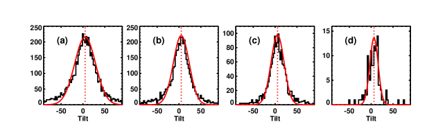
Figure 1: Histograms (2.5^∘ bins) of the tilt angle distributions for different ranges of umbral area (Kodaikanal data). Red curves show Gaussian fits. From (a) to (d), the umbra area ranges are 10–15.8, 25.1–39.8, 63.1–100, and 158.5–251.2 in $\mu$H, respectively.

Consistent with Stenflo & Kosovichev (2012), we find that the tilt angle scatter strongly decreases with increasing sunspot group area (see Table LABEL:tab:tilts_obs). In contrast to Stenflo & Kosovichev (2012), we also find that the mean tilt angle increases somewhat with sunspot group area, but only for the Kodaikanal data, so that the relevance of this trend is unclear. Hereafter we therefore do not consider a size dependence of the mean tilt angle, but only its the latitudinal dependence (Joy’s Law). Figure 1 shows four of the tilt angle distributions in $2.5^{\circ}$ bins from Kodaikanal record together with the Gaussian fits (red curves) from which the values given in Table LABEL:tab:tilts_obs were derived. Figure 2 shows the tilt angle scatter, $\sigma_{\alpha}$, as a function of umbral area, $A_{U}$. The error bars indicate one-sigma error estimates. The data shown in Figure 2 can be represented by the expression

$$\sigma_{\alpha}=-11*\log(A_{U})+35.$$ (1)

We also studied the latitude dependence of the scatter. Table LABEL:tab:lat shows that there is no significant latitudinal dependence of the scatter on the tilt angle. These results are consistent with the visual impression given by Figure 2 of Fisher et al. (1995) where a strong dependence of the HWHM of the distributions with respect to area can be seen, with no obvious dependence on latitude.

3 Model description

3.1 Surface flux transport model

The surface flux transport (SFT) model (see the review by Mackay & Yeates, 2012) describes the evolution of the large-scale magnetic flux distribution at the solar surface as a combined result of the emergence of bipolar magnetic regions, a random walk due to supergranular flows, and the transport by large-scale surface flows (e.g., Wang et al., 1989; van Ballegooijen et al., 1998; Mackay et al., 2002; Schrijver et al., 2002; Baumann et al., 2004). The relevant equation is

$$\frac{\partial B}{\partial t}= - \omega(\theta)\frac{\partial B}{\partial\phi}-\frac{1}{R_{\odot}\sin\theta}\frac{\partial}{\partial\theta}\left[\upsilon(\theta)B\sin\theta\right]$$ (2)

$$+ \frac{\eta}{R_{\odot}^{2}}\left[\frac{1}{\sin\theta}\frac{\partial}{\partial\theta}\left(\sin\theta\frac{\partial B}{\partial\theta}\right)+\frac{1}{\sin^{2}\theta}\frac{\partial^{2}B}{\partial\phi^{2}}\right]$$

$$+ S(\theta,\phi,t),$$

where $B$ is the radial component of the magnetic field, $\theta$ is the heliographic colatitude ($\lambda=\pi/2-\theta$ is the latitude), and $\phi$ is the heliographic longitude. For the surface differential rotation, $\omega(\theta)$, we use the profile given by Snodgrass (1983) $\omega(\theta)=13.38-2.30\cos^{2}\theta-1.62\cos^{4}\theta$-13.2 (in deg day ^-1). The surface meridional flow, $\upsilon(\theta)$, is described by the profile suggested by van Ballegooijen et al. (1998), i.e.,

$$\upsilon(\lambda)=\left\{\begin{array}[]{l l}\upsilon_{0}\sin(180^{\circ}\lambda/\lambda_{0})&|\lambda|\leq\lambda_{0}\\ 0&\textrm{otherwise},\end{array}\right.$$ (3)

with $\upsilon_{0}=11$ ms^-1 and $\lambda_{0}=75^{\circ}$. The turbulent diffusivity that models the random walk of magnetic features associated with supergranulation is taken as $\eta=250\,$km²s^-1. This value is in the middle of the range given by Schrijver & Zwaan (2000) (see also Jiang et al., 2013a). The source of the magnetic flux, $S(\theta,\phi,t)$, describing the emergence of the sunspot groups is discussed in the subsequent section.

For the numerical simulations we used the code originally developed by Baumann et al. (2004). The magnetic field is expressed in terms of spherical harmonics up to $l$ = 63. A fourth-order Runge-Kutta method is used for time stepping.

3.2 Sources of magnetic flux

We follow the method described by Cameron et al. (2010) and Jiang et al. (2011b) to generate the source term, $S(\theta,\phi,t)$, from the RGO sunspot record. In brief, each observed sunspot group is regarded as a bipolar magnetic region (BMR) with modified Gaussian distributions for the preceding and following parts (Baumann et al., 2004). Polarities are chosen according to Hale’s laws, taken into account the cycle overlap around activity minima. Each BMR is introduced into the SFT simulation at the time of maximum sunspot area of the corresponding sunspot group.

We use the RGO record since it is by far the longest and most complete in terms of coverage of sunspot groups. The disadvantage of RGO data, however, is the absence of information concerning the tilt angles. We therefore assign the tilt angle for each BMR according to the relation determined by Jiang et al. (2011a),

$$\alpha=0.7\,T_{n}\sqrt{|\lambda|}+\epsilon,$$ (4)

where $T_{n}$ ($n$ is the cycle number) represents the systematic variation of the mean tilt angle between solar cycles, as determined by Jiang et al. (2011a) (see their Figure 11 and Equation 15). In the cycles studied here, we have $T_{14}=1.5$, $T_{17}=1.3$ and $T_{19}=1.0$. Combining the RGO sunspot area records with $T_{n}$ for different cycles, the study by Cameron et al. (2010) can be extended back to 1874. The factor 0.7 was introduced and calibrated by Cameron et al. (2010) to reproduce the observed ratio between the maxima and minima of the open heliospheric flux. It possibly results from the reduction of the tilt angles by near-surface inflows towards sunspot groups (Gizon, 2004; Jiang et al., 2010).

The scatter of the tilt angles is modeled by $\epsilon$ in Equation (4), which is drawn from random distributions consistent with the observationally inferred standard deviations in the various $A_{U}$ bins (cf. Table LABEL:tab:tilts_obs). We assume $\epsilon$ for each BMR to be an independent realization of a random process with a Gaussian distribution with zero mean and a half width according to the relationship between scatter and umbral area given by Equation (1).

We first study cycle 17 (1933.8-1944.2), which has a medium cycle amplitude during the period of RGO data, with a maximum $R_{g}=123$ of the 12-month running mean of the group sunspot number. We discuss the results for cycle 19 (the strongest cycle during the period covered by the RGO data) and cycle 14 (the weakest cycle) in Section 4.5. As the initial condition for the SFT simulations, we take the field distribution at the time 1933.8 from the extended simulation of Cameron et al. (2010), where we use the values of $T_{n}$ according to its relationship to cycle strength (in the form given by Jiang et al., 2011a). Since it takes roughly 2 years for low-latitude magnetic flux to be transported to the poles, we run the SFT simulations until 2 years after the minimum between cycles 17 and 18, i.e., until 1946.2. Similar procedures are followed for cycles 14 and 19.

3.3 Averaged quantities

The output of the SFT simulations is the radial component of the magnetic field at the solar surface as a function of colatitude, longitude and time, $B(\theta,\phi,t)$. A more compact representation of the results is obtained by considering the longitudinally averaged field as a function of colatitude and time,

$$\left\langle B\right\rangle(\theta,t)=\frac{1}{2\pi}\int_{0}^{360}B(\theta,\phi,t)d\phi,$$ (5)

which yields a “magnetic butterfly diagram”. Several one-dimensional time series can be constructed from $\left\langle B\right\rangle(\theta,t)$ by performing weighted integrals over various (co)latitude ranges. Among these are the polar fields of each hemisphere, which we here define as the average (signed) field poleward of $\pm 75^{\circ}$ latitude in each hemisphere. For the north polar field we thus write

$$B_{\rm NP}=\int_{0}^{15}\left\langle B\right\rangle(\theta,t)\sin\theta d\theta\left/\int_{0}^{15}\sin\theta d\theta\right.,$$ (6)

and analogous for the south polar field, $B_{\rm SP}$. Other relevant quantities are the axial dipole moment,

$$D(t)=\frac{3}{2}\int_{0}^{180}\left\langle B\right\rangle(\theta,t)\cos\theta\sin\theta d\theta,$$ (7)

the low-latitude contribution to the dipole moment,

$$D_{<55}(t)=\frac{3}{2}\int_{35}^{145}\left\langle B\right\rangle(\theta,t)\cos\theta\sin\theta d\theta,$$ (8)

and the quantity

$$S_{<55}(t)=\int_{35}^{145}|\left\langle B\right\rangle(\theta,t)|\sin\theta d\theta\left/\int_{35}^{145}\sin\theta d\theta\right.,$$ (9)

which we introduce as a measure of the structure in the mid- and low-latitude part of the magnetic butterfly diagram.

4 Results

We study the effect of the scatter in the tilt angles on the evolution of the Sun’s large-scale magnetic field by comparing simulations with and without the scatter.

4.1 Evolution without tilt angle scatter

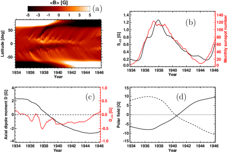
Figure 3: Evolution of the simulated large-scale magnetic field during cycle 17 for the case without tilt angle scatter. (a): time-latitude diagram of $\langle B\rangle$; (b): low-latitude structure, $S_{<55}$ (black), and observed sunspot number (red); (c): total axial dipole moment, $D$ (black), and contribution to $D$ of the latitudes below $\pm 55^{\circ}$ (red); (d): North (dashed) and South (solid) polar field. For definitions of these quantities, see Eqs. (5) to (9).

Figure 3 shows results of the simulation for cycle 17 with no scatter in the tilt angles, i.e., $\epsilon=0$ in Equation (4). Panel (a) shows the magnetic butterfly diagram, i.e., the time-latitude plot of $\langle B\rangle$. Poleward surges of magnetic flux in both hemispheres illustrate the transport magnetic flux with following polarity (opposite to the polarity of the polar field during rise phase of the cycle) from the activity belt to the poles. They reverse the old polar field of cycle 16 and build up the polar field of cycle 17. The time evolution of $S_{<55}(t)$, which represents the amount of structure in the magnetic butterfly diagram at mid and low latitudes, is given in panel (b) along with the observed sunspot number (in red). The value of $S_{<55}(t)$ at a given time is mainly determined by the product of area and modulus of the tilt of the BMRs present. Its evolution roughly follows the solar cycle and peaks around the cycle maximum in 1937.9. Panel (c) shows the evolution of the total axial dipole moment, $D$ (black curve), and the contribution of the low-latitude flux, $D_{<55}$ (red curve). During the initial phase of the simulation, the positive north polar field and negative south polar field correspond to a positive dipole moment. BMRs emerging in the course of cycle 17 then contribute negative dipole moments at low latitude as seen in $D_{<55}$ (the positive values during the beginning of the cycle are due to cycle overlap). With the subsequent transport towards the poles, the global dipole moment decreases and reverses around 1938.5. It peaks just after the cycle minimum (1944.6). Panel (d) shows the corresponding evolution of the polar fields, which reach their (unsigned) maxima about 2 years after solar minimum. Note that the timing of the polar field reversals depends on the definition of the ‘polar cap’ and on whether the radial component or the line-of-sight component with respect to the ecliptic of the magnetic field is considered. The difference can amount up to two years (Jiang et al., 2013b).

The second column in Table LABEL:tab:comparison gives numerical values for the maxima of the quantities discussed above. The asymmetry of the polar fields is due to the hemispherically asymmetric sunspot emergence.

4.2 Evolution with tilt angle scatter

We evaluated the effects of the tilt angle scatter by performing SFT simulations of cycle 17 for which each emerging BMR was associated with a random perturbation of the tilt angle, $\epsilon$, according to Equation (4). The values for $\epsilon$ were taken from a Gaussian distribution with zero mean and a standard deviation $\sigma_{\alpha}$ based on Equation (1). We carried out 50 simulation runs with different realizations of $\epsilon$. The standard deviations, associated with 50 random realizations, of the quantities defined in Section 3.3 reflect the effects of the scatter in sunspot group tilt angles on the large-scale field.

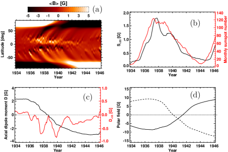
Figure 4: Similar to Figure 3, but for one simulation run (out of 50) with random scatter of the tilt angles according to the observed distributions. This example develops a similar dipole field as the case without the tilt angle scatter.

Figure 4 illustrates the result for one of these runs. The simulated magnetic butterfly diagram, shown in panel (a), appears more ‘grainy’ than the corresponding plot in Figure 3, which is the result of some BMRs emerging with randomly occurring large tilt angles. This graininess is represented by an increase of the quantity $S_{<55}$ by about 40% compared to the case without tilt angle scatter (cf. panel (b) in Figure 3). In the case of SFT simulations without tilt angle scatter, the ratio of the net magnetic fluxes in the activity belts and in the polar regions is usually lower than in the observations. Examples are Figure 6 of Schüssler & Baumann (2006) and Figure 3 of Yeates (2014). The tilt angle scatter increases the averaged net flux at the low latitudes without increasing the net flux at high latitudes. There are also more poleward surges of opposite-polarity flux. The magnetic butterfly diagrams for simulations with tilt angle scatter are therefore more similar to their observed counterpart for the last 3 cycles (see, e.g., Hathaway, 2010).

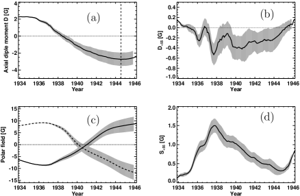
Figure 5: Evolution of various quantities for simulations including random scatter of the tilt angles. Solid curves show averages of 50 simulations with different sets of random numbers while gray shades indicate the corresponding standard deviations. (a): total axial dipole moment, $D$; (b): contribution to $D$ of the latitudes below $\pm 55^{\circ}$; (c): North (dashed) and South (solid) polar field; (d): mean net flux density within $\pm 55^{\circ}$ latitude. For definitions of these quantities, see Eqs. (6) to (9).

For the case shown in Figure 4, the dipole field in panel (c) and the polar field in panel (d) exhibit a similar time evolution as in the case without the tilt scatter. However, this is not a general feature as can be seen in Figure 5, which shows the averages (solid and dashed curves) and the standard deviations (grey shades) of these quantities for the 50 SFT simulations with tilt angle scatter. Panel (a) gives the time evolution of the axial dipole moment, $D$. The average curve is close to the case without the tilt angle scatter shown in Figure 3. Since the dipole moment is built up from the accumulated contributions of emerging BMRs, the standard deviation increases with time. It starts at zero since the initial condition was the same for all runs. At the time of maximum dipole moment (indicated by the dashed vertical line), the standard deviation due to the random scatter of the tilt angles amounts to 0.78G, which is about 30% of the average value at the end of cycle 17. The relative variation (30%) depends on the mean dipole moment at the end of the cycle (which is correlated with the strength of the following cycle, Jiang et al., 2007).

The contribution of the lower latitudes to the axial dipole moment, $D_{<55}$, shown in panel (b) of Figure 5 is strongly affected by the tilt angle scatter. Finally, panel (d) shows the quantity $S_{<55}(t)$, which represents the amount of structure in the magnetic butterfly diagram. The maximum of its average time profile is about 20% higher than for the case without the tilt scatter. This results from strongly tilted BMRs, which occasionally appear in the runs with scatter and contribute significantly to $S_{<55}(t)$. A comparison between the values for the various quantities discussed above for the cases with and without scatter is given in Table LABEL:tab:comparison.

4.3 Dependence on sunspot group size

In order to study the dependence of the effect of tilt angle scatter on group size, we divided the sunspot groups of cycle 17 into 5 samples of approximately equal total umbral area. We then carried out $5\times 50$ SFT simulations for which the random component of the tilt angle, $\epsilon$, was only introduced in one of these samples while the others had $\epsilon=0$.

Table LABEL:tab:diff_size summarizes the results of these simulations, where $N$ denotes the number of the sunspot groups in each bin. We see that the contribution of each bin to the standard deviation of the axial dipole moment scales roughly as $1/\sqrt{N}$, so that the effect of the tilt angle scatter decreases systematically for the (more numerous) small groups. We therefore expect that the effect of the scatter in the tilt angles of the abundant ephemeral regions is negligible.

4.4 Dependence on sunspot group latitude

In order to study how the effect of the tilt angle scatter depends on the latitude of emerging BMRs, we divided the sunspot groups of cycle 17 in 5 latitude bins. We then carried out $5\times 50$ SFT simulations for which the tilt angle scatter was only applied to the groups belonging to one of these bins. The bins and the results of these simulations are shown in Table LABEL:tab:diff_lati.

Similar to the size dependence discussed in the preceding subsection, we find that the averages of the maximum values of the dipole moment and of the polar fields are almost unaffected (cf. Table LABEL:tab:comparison). However, the latitude dependence of the standard deviations of the axial dipole and the polar fields, i.e., their uncertainty due to the random component, is quite strong: sunspot groups emerging below 15^∘ contribute much more strongly to the uncertainties than those appearing in higher latitudes. As explained in the above subsection, the uncertainties result from a combination of two factors: the number of sunspot groups $N$ in a given latitude bin and their individual contribution to the dipole and polar fields. Although there are 3 times less sunspot groups in the 0^∘-5^∘ bin than that in the 10^∘-15^∘ bin, both latitude ranges contribute similarly to the standard deviation of the dipole moment. This reflects the fact that individual sunspot groups at lower latitudes affect the evolution of the dipole field more strongly.

To illustrate the strong dependence of the uncertainty on emergence latitude, we performed SFT simulations with single BMRs initially placed at different latitudes. We chose a sunspot group with $A_{U}=1000$ $\mu$H, corresponding to a total magnetic flux of 6$\times 10^{21}$Mx, and assumed a large tilt angle of 80^∘. We considered cases where the BMR was inserted at latitudes between 0^∘ and 40^∘, in steps of 10^∘.

The left panel of Figure 6 shows the evolution of the axial dipole moment for the various emergence latitudes. For cross-equator emergence (0^∘), the centroids of the two polarities are initially located at about $\pm 4.3^{\circ}$ latitude. Advection by the meridional flow in each hemisphere separates the polarities and increases the dipole moment. At the same time, about half of the magnetic flux diffuses across the equator, where it cancels with opposite-polarity flux. The remaining flux is eventually transported to the poles and the dipole moment reaches a plateau of 0.9 G, corresponding to polar fields of $\pm 3.7$ G. These values represent about 20% of the simulated dipole and polar fields generated by all recorded sunspot groups of cycle 17. At the other extreme, the axial dipole moments due to BMRs emerging at 30^∘ or 40^∘ steadily decay as both polarities are swept together towards the pole and cancel there, while only a negligible amount of magnetic flux is transported across the equator. The intermediate cases of emergence at 10^∘ and 20^∘, show a mixture of the two types of behavior. The right panel of Figure 6 shows the relation between the final axial dipole moment and the latitudinal location of the BMR with a given magnetic flux and tilt angle. The behaviour corresponds to a Gaussian distribution with a HWHM in latitude of 8.8^∘ (solid curve). The final dipole field is roughly proportional to the BMR size and the sine of the tilt angle (Baumann et al., 2004).

4.5 Dependence of the scatter in the dipole moment at the end of a cycle on the strength of the cycle

We have also carried out the above analysis for cycle 14 (the weakest cycle covered by RGO, 2222 sunspot groups) and for cycle 19 (the strongest cycle, 4648 sunspot groups). The results are shown in Table LABEL:tab:cycles14-19. For our reference cycle 17 (3579 sunspot groups) the scatter in the tilt angle leads to a standard deviation of 0.78G in the resulting axial dipole moment at the end of the cycle. The substantially weaker cycle 14 produces a dipole field with a standard deviation of 0.81G, and the much stronger cycle 19 is associated with a standard deviation of 0.76G. The uncertainty of the dipole moment at the end of a cycle resulting from the random tilt angle scatter is thus almost unrelated to the strength of the cycle. This can be understood because stronger cycles have higher mean latitudes (Solanki et al., 2008; Jiang et al., 2011a) where the scatter introduces less noise into the dipole moment (see Section 4.4). The cycle dependence of the latitude distribution of sunspot groups is also presented in Table LABEL:tab:cycles14-19, where we see that the differences between the two cycles decreases at low latitudes. According to the results in the above two subsections, only the scatter in the tilt angles of large sunspot groups at low latitudes has large effects on the uncertainties of the axial dipole moment.

As shown in Table LABEL:tab:cycles14-19, the average dipole moments for cycles 14 and 19 are 2.01G and 2.21G, respectively. The standard deviations correspond to 40% and 34%, respectively, of these values. The percentages are somewhat higher than the value of 28% for cycle 17., but this is mainly due to the differing strengths of the dipole moment at the end of the three cycles rather than to a change in the standard deviation introduced by the scatter. In absolute terms, the scatter in the dipole moments for cycles 14, 17 and 19 are almost the same: 0.8G, 0.78G, and 0.75G, respectively.

Table LABEL:tab:cycles14-19 also shows that the near-equator emergence dominates the scatter of the dipole moments for both weak and strong cycles: sunspot groups emerging below 15^∘ contribute most to the standard deviation of the axial dipole moment. Similar to the results for cycle 17 given in Table LABEL:tab:diff_lati, the combination of the number of sunspot groups in a given bin and the latitude dependence of their individual contributions leads to a maximum of the standard deviation in the 5^∘-10^∘ bin.

Figure 7 shows the averages (solid curves) and the standard deviations (grey shades) of the axial dipole moment and $S_{n}$, the mean unsigned latitudinally averaged (signed) flux densities in the latitudinal range from $-55^{\circ}$ to $55^{\circ}$ for cycles 14 and 19.

5 Summary

We have measured the tilt scatter based on the Kodaikanal and Mount Wilson tilt angle data and studied the effects of this scatter on the evolution of the solar surface field using the surface flux transport simulations with flux input based upon the recorded sunspot groups.

The analysis of the tilt angle data shows that the average tilt angles have a weak trend to increase with the sunspot group size, while the standard deviations significantly decrease. The relation between the standard deviations and the sunspot group size can be well fitted by a linear logarithmic function.

The simulations including the tilt scatter of the sunspot groups show that the scatter has a significant effect on the evolution of the large-scale magnetic field at the solar surface. The longitudinal averaged magnetic flux at low latitudes is increased with a more grainy structure generated by sunspot groups with large tilt angles. On the average, the net unsigned magnetic flux in the magnetic butterfly diagram at latitudes below 55^∘ is increased by about 20%. Including the tilt angle scatter makes the simulated magnetic butterfly diagram thus better consistent with the observations: the ratio of the unsigned magnetic flux between the low and the high latitudes is increased and more poleward surges of opposite-polarity flux are generated.

The axial dipole moment and the polar fields during solar activity minimum of cycle 17 may change by about $\pm 30$% (compared to its mean value) owing to random fluctuations of the tilt angles within the range indicated by observations. This is consistent with the results of Baumann et al. (2004) for artificial solar cycles. The standard deviation of the axial dipole field introduced by the scatter in the tilt angle is almost independent of the strength of the cycle. The effects of the tilt scatter on the large-scale field at the solar surface mainly result from large sunspot groups emerging at low latitudes.

We may conclude from these results that, in the framework of Babcock-Leighton dynamo models, the random component introduced by the tilt angle scatter has a significant impact on the variability of the solar cycle strength. Since the polar fields (or axial dipole moment of the surface field) that are built up during a cycle represent the poloidal field source for the following cycle, the fluctuations due to the tilt angle scatter directly affect the strength of this cycle. Even a single big sunspot group with large tilt appearing near the equator may in this way significantly affect the strength of the next cycle (cf. Cameron et al., 2013). This obviously sets stringent limits on the predictability of future activity cycles.

Figure 6: Left panel: time evolution of the axial dipole moment resulting from a single BMR with a total flux of 6$\times 10^{21}$ Mx and tilt angle 80^∘, for various emergence latitudes; Right panel: relation between the eventual equilibrium axial dipole moment and the latitudinal location of a BMR with given flux, F, and tilt angle, $\alpha$. The points are the results from SFT simulations for different BMRs emerging at different latitudes. The solid curve is the Gaussian fit of the form $\exp(-\lambda^{2}/110)$.

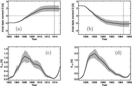
Figure 7: Results for cycle 14 (left panels) and cycle 19 (right panels) for simulations including random scatter of the tilt angles. Panels (a) and (b): total axial dipole moment; Panels (c) and (d): mean unsigned latitudinally averaged (signed) flux density within $\pm 55^{\circ}$ latitude.

Table 1: Tilt angles of sunspot groups from the Kodaikanal (KOD) and Mount Wilson (MWO) records for various ranges of umbral area, $A_{U}$. $N$: number of sunspot groups; $\left\langle\alpha\right\rangle$: average tilt angle (in degrees); $\sigma_{\alpha}$ standard deviation.

		KOD			MWO
$A_{U}$ [$\mu$H]	$N$	$\left\langle\alpha\right\rangle$	$\sigma_{\alpha}$	$N$	$\left\langle\alpha\right\rangle$	$\sigma_{\alpha}$
0.0 – 6.3	6801	4.75$\pm$0.91	29.97$\pm$0.76	6660	4.63$\pm$0.89	30.23$\pm$0.75
6.3 – 10.0	4557	4.56$\pm$0.88	25.63$\pm$0.73	3939	5.25$\pm$0.89	24.64$\pm$0.73
10.0 – 15.8	5196	4.96$\pm$0.65	24.02$\pm$0.53	4686	4.94$\pm$0.75	23.13$\pm$0.61
15.8 – 25.1	5054	5.04$\pm$0.69	20.78$\pm$0.56	4758	5.36$\pm$0.57	19.89$\pm$0.46
25.1 – 39.8	4014	5.11$\pm$0.53	18.16$\pm$0.44	3822	5.51$\pm$0.57	17.17$\pm$0.47
39.8 – 63.1	2692	6.18$\pm$0.47	15.55$\pm$0.39	2583	5.14$\pm$0.48	14.80$\pm$0.39
63.1 – 100.0	1469	5.59$\pm$0.45	14.94$\pm$0.37	1293	5.24$\pm$0.32	13.06$\pm$0.26
100.0 – 158.5	532	6.78$\pm$0.38	10.24$\pm$0.31	400	5.06$\pm$0.43	10.57$\pm$0.35
158.5 – 251.2	131	6.53$\pm$0.68	9.55$\pm$0.55	84	5.63$\pm$0.66	8.29$\pm$0.54
251.2 – max	30	2.62$\pm$2.50	14.67$\pm$2.04	20	4.26$\pm$1.02	6.89$\pm$0.83

Table 2: Standard deviation of the tilt angle scatter of sunspot groups from the Kodaikanal (KOD) and Mount Wilson (MWO) records for various latitudinal ranges.

	0.0∘ – 10.0∘	10.0∘ – 15.0∘	15.0∘ – 20.0∘	20.0∘ – max
KOD	30.8	29.1	30.2	31.1
MWO	30.0	29.6	30.2	30.9

Table 3: Maximum values (in G) of various quantities from simulation runs without and with tilt angle scatter from 50 random realizations. $D$: axial dipole moment; $B_{\rm NP}$ and $B_{\rm SP}$: north and south polar field; $S_{<55}$: mean flux of the magnetic butterfly diagram among $\pm 55^{\circ}$ latitudes. For definitions, see Eqs. (6) to (9).

	without scatter	with scatter
$|D|$	$2.68$	$2.73\pm 0.78$
$|B_{\rm NP}|$	$9.46$	$8.82\pm 3.05$
$|B_{\rm SP}|$	$10.82$	$12.02\pm 3.18$
$S_{<55}$	$1.27$	$1.50\pm 0.18$

Table 4: Results (in G) for tilt angle scatter restricted to sunspot groups within a given range of umbral area, $A_{U}$ (in $\mu$H). $N$ denotes the number of the sunspot groups in each bin.

$A_{U}$ range	0 – 28	28 – 56	56 – 94	94 – 160	160 – max
$|D|$	$2.67\pm 0.16$	$2.75\pm 0.24$	$2.69\pm 0.33$	$2.69\pm 0.45$	$2.81\pm 0.48$
$|B_{\rm NP}|$	$8.73\pm 0.64$	$8.98\pm 0.95$	$8.84\pm 1.27$	$8.76\pm 1.83$	$9.14\pm 1.74$
$|B_{\rm SP}|$	$11.49\pm 0.57$	$11.83\pm 0.94$	$11.53\pm 1.31$	$11.61\pm 1.72$	$11.99\pm 2.01$
$N$	2496	514	294	179	84

Table 5: Results (in G) for tilt angle scatter restricted to sunspot groups emerging within a given latitude range.

$|\lambda|$ range	25∘ – max	15∘ – 25∘	10∘ – 15∘	5∘ – 10∘	0∘ – 5∘
$|D|$	$2.72\pm 0.01$	$2.72\pm 0.08$	$2.71\pm 0.36$	$2.74\pm 0.57$	$2.71\pm 0.35$
$|B_{\rm NP}|$	$8.91\pm 0.07$	$8.95\pm 0.39$	$8.86\pm 1.42$	$8.84\pm 2.20$	$8.89\pm 1.26$
$|B_{\rm SP}|$	$11.63\pm 0.02$	$11.66\pm 0.37$	$11.68\pm 1.67$	$11.81\pm 2.20$	$11.66\pm 1.20$
$N$	436	1249	932	729	223

Table 6: Results for cycles 14 and 19 with the tilt angle scatter restricted to sunspot groups emerging within a given latitude range. $D_{14}$ and $D_{19}$: dipole moments; $N_{14}$ and $N_{19}$: numbers of the sunspot groups in each bin.

$|\lambda|$ range	0∘ – max	25∘ – max	15∘ – 25∘	10∘ – 15∘	5∘ – 10∘	0∘ – 5∘
$|D_{14}|$	$2.01\pm 0.81$	$2.09\pm 0.003$	$2.09\pm 0.06$	$2.11\pm 0.24$	$2.09\pm 0.60$	$2.01\pm 0.37$
$N_{14}$	$2222$	73	770	648	557	174
$|D_{19}|$	$2.21\pm 0.76$	$2.27\pm 0.004$	$2.28\pm 0.13$	$2.20\pm 0.35$	$2.27\pm 0.63$	$2.27\pm 0.43$
$N_{19}$	$4648$	789	1719	1095	764	281

References

- Baumann et al. (2004) Baumann, I., Schmitt, D., Schüssler, M., & Solanki, S. K. 2004, A&A, 426, 1075
- Caligari et al. (1995) Caligari, P., Moreno-Insertis, F., & Schüssler, M. 1995, ApJ, 441, 886
- Cameron et al. (2014) Cameron, R., Jiang, J., S. M., & Gizon, L. 2014, J. Geophys. Res. Space Physics, 119, 9
- Cameron et al. (2013) Cameron, R. H., Dasi-Espuig, M., Jiang, J., et al. 2013, A&A, 557, A141
- Cameron et al. (2010) Cameron, R. H., Jiang, J., Schmitt, D., & Schüssler, M. 2010, ApJ, 719, 264
- Charbonneau (2010) Charbonneau, P. 2010, Living Reviews in Solar Physics, 7, 3, http://www.livingreviews.org/lrsp-2010-3
- Charbonneau & Dikpati (2000) Charbonneau, P., & Dikpati, M. 2000, ApJ, 543, 1027
- Dasi-Espuig et al. (2010) Dasi-Espuig, M., Solanki, S. K., Krivova, N. A., Cameron, R., & Peñuela, T. 2010, A&A, 518, A7
- D’Silva & Choudhuri (1993) D’Silva, S., & Choudhuri, A. R. 1993, A&A, 272, 621
- Fan (2009) Fan, Y. 2009, Living Reviews in Solar Physics, 6, 4, http://www.livingreviews.org/lrsp-2009-4, doi:10.12942/lrsp-2009-4
- Fan et al. (1993) Fan, Y., Fisher, G. H., & Deluca, E. E. 1993, ApJ, 405, 390
- Fisher et al. (1995) Fisher, G. H., Fan, Y., & Howard, R. F. 1995, ApJ, 438, 463
- Gizon (2004) Gizon, L. 2004, Sol. Phys., 224, 217
- Hale et al. (1919) Hale, G. E., Ellerman, F., Nicholson, S. B., & Joy, A. H. 1919, ApJ, 49, 153
- Hathaway (2010) Hathaway, D. H. 2010, Living Reviews in Solar Physics, 7, 1, http://www.livingreviews.org/lrsp-2010-1, doi:10.12942/lrsp-2010-1
- Howard et al. (1984) Howard, R., Gilman, P. I., & Gilman, P. A. 1984, ApJ, 283, 373
- Howard (1991a) Howard, R. F. 1991a, Sol. Phys., 136, 251
- Howard (1991b) —. 1991b, Sol. Phys., 132, 49
- Howard (1991c) —. 1991c, Sol. Phys., 132, 257
- Howard (1996) —. 1996, Sol. Phys., 167, 95
- Jiang et al. (2013a) Jiang, J., Cameron, R. H., Schmitt, D., & Işık, E. 2013a, A&A, 553, A128
- Jiang et al. (2011a) Jiang, J., Cameron, R. H., Schmitt, D., & Schüssler, M. 2011a, A&A, 528, A82
- Jiang et al. (2011b) —. 2011b, A&A, 528, A83
- Jiang et al. (2013b) —. 2013b, Space Sci. Rev., 176, 289
- Jiang et al. (2007) Jiang, J., Chatterjee, P., & Choudhuri, A. R. 2007, MNRAS, 381, 1527
- Jiang et al. (2010) Jiang, J., Işik, E., Cameron, R. H., Schmitt, D., & Schüssler, M. 2010, ApJ, 717, 597
- Li & Ulrich (2012) Li, J., & Ulrich, R. K. 2012, ApJ, 758, 115
- Longcope & Fisher (1996) Longcope, D. W., & Fisher, G. H. 1996, ApJ, 458, 380
- Mackay & Yeates (2012) Mackay, D., & Yeates, A. 2012, Living Reviews in Solar Physics, 9, 6, http://www.livingreviews.org/lrsp-2012-6, arXiv:1211.6545
- Mackay et al. (2002) Mackay, D. H., Priest, E. R., & Lockwood, M. 2002, Sol. Phys., 209, 287
- McClintock & Norton (2013) McClintock, B. H., & Norton, A. A. 2013, Sol. Phys., 287, 215
- Olemskoy et al. (2013) Olemskoy, S. V., Choudhuri, A. R., & Kitchatinov, L. L. 2013, Astronomy Reports, 57, 458
- Ravindra et al. (2013) Ravindra, B., Priya, T. G., Amareswari, K., et al. 2013, A&A, 550, A19
- Schrijver et al. (2002) Schrijver, C. J., De Rosa, M. L., & Title, A. M. 2002, ApJ, 577, 1006
- Schrijver & Zwaan (2000) Schrijver, C. J., & Zwaan, C. 2000, Solar and Stellar Magnetic Activity (Cambridge University Press)
- Schüssler & Baumann (2006) Schüssler, M., & Baumann, I. 2006, A&A, 459, 945
- Sivaraman et al. (2007) Sivaraman, K. R., Gokhale, M. H., Sivaraman, H., Gupta, S. S., & Howard, R. F. 2007, ApJ, 657, 592
- Sivaraman et al. (1999) Sivaraman, K. R., Gupta, S. S., & Howard, R. F. 1999, Sol. Phys., 189, 69
- Solanki et al. (2008) Solanki, S. K., Wenzler, T., & Schmitt, D. 2008, A&A, 483, 623
- Stenflo & Kosovichev (2012) Stenflo, J. O., & Kosovichev, A. G. 2012, ApJ, 745, 129
- Tian et al. (2003) Tian, L., Liu, Y., & Wang, H. 2003, Sol. Phys., 215, 281
- Tian et al. (1999) Tian, L., Zhang, H., Tong, Y., & Jing, H. 1999, Sol. Phys., 189, 305
- van Ballegooijen et al. (1998) van Ballegooijen, A. A., Cartledge, N. P., & Priest, E. R. 1998, ApJ, 501, 866
- Wang et al. (1989) Wang, Y.-M., Nash, A. G., & Sheeley, Jr., N. R. 1989, ApJ, 347, 529
- Wang & Sheeley (1989) Wang, Y.-M., & Sheeley, Jr., N. R. 1989, Sol. Phys., 124, 81
- Weber et al. (2011) Weber, M. A., Fan, Y., & Miesch, M. S. 2011, ApJ, 741, 11
- Weber et al. (2013) —. 2013, Sol. Phys., 287, 239
- Yeates (2014) Yeates, A. R. 2014, Sol. Phys., 289, 631