The cause of the weak solar cycle 24

Abstract

The ongoing 11-year cycle of solar activity is considerably less vigorous than the three cycles before. It was preceded by a very deep activity minimum with a low polar magnetic flux, the source of the toroidal field responsible for solar magnetic activity in the subsequent cycle. Simulation of the evolution of the solar surface field shows that the weak polar fields and thus the weakness of the present cycle 24 are mainly caused by a number of bigger bipolar regions emerging at low latitudes with a ‘wrong’ (i.e., opposite to the majority for this cycle) orientation of their magnetic polarities in the North-South direction, which impaired the growth of the polar field. These regions had a particularly strong effect since they emerged within $\pm 10^{\circ}$ latitude from the solar equator.

1 Introduction

Solar activity, as manifested by sunspots and bipolar magnetic regions at the solar surface, by energy release in flares, eruptions, coronal mass ejections, and energetic particles, varies cyclically with a (quasi-)period of about 11 years (Hathaway, 2010). Activity cycles differ significantly with regard to their length and strength. The present cycle is among the weaker ones, particularly if compared with the sequence of strong cycles during the second half of the 20th century. Cycle 24 was preceded by an unusually extended period of very low activity (Russell et al., 2010), weak polar magnetic field (Muñoz-Jaramillo et al., 2012), and low heliospheric open flux (Smith & Balogh, 2008; Owens & Forsyth, 2013). This is consistent with the empirical correlation of the polar field around solar activity minimum with the strength of the subsequent cycle (Wang & Sheeley, 2009). This correlation reflects the role of poloidal magnetic flux connected to the polar fields as the dominant poloidal source of the toroidal flux generated by differential rotation in the solar interior (Cameron & Schüssler, 2015), whose emergence at the surface during the subsequent 11-year cycle leads to the various manifestations of solar activity.

Generally, the observed large-scale solar surface field is well represented by Surface Flux Transport (SFT) simulations (Wang et al., 1989; Sheeley, 2005; Mackay & Yeates, 2012; Jiang et al., 2014b), which address the evolution of the magnetic field as a result of the emergence of bipolar magnetic regions (sunspot groups) and the subsequent transport of magnetic flux by near-surface plasma flows (convection, differential rotation, poleward meridional flow). Such models showed that the polar fields are reversed and built up by preferred flux transport of one polarity across the equator as a result of the systematic tilt of bipolar sunspot groups with respect to the direction of rotation. The strength of the polar fields mainly depends on the tilt angle, the distribution of emerging flux in heliographic latitude, and the speed of the meridional flow (Baumann et al., 2004). SFT simulations reproduce the polar fields (as regularly measured directly since 1976 and inferred from geomagnetic and solar proxies measured since the 19th century) relatively well for the cycles before cycle 23. However, unless they are continuously adjusted by data assimilation from observations (Upton & Hathaway, 2014b), such simulations so far could not reproduce the very weak polar field during the declining phase and activity minimum of cycle 23 (Jiang et al., 2010; Yeates, 2014; Upton & Hathaway, 2014a). Suitable ad-hoc variations of the meridional flow were considered as a possible remedy (Schrijver & Liu, 2008; Wang & Sheeley, 2009; Nandy et al., 2011; Jiang et al., 2013), but there is no empirical basis for changes of the kind required by these models (González Hernández et al., 2008; Hathaway & Rightmire, 2010; Cameron & Schüssler, 2010).

While systematic variations of the tilt angles of sunspot groups (Cameron et al., 2010) were found to be an unlikely cause of the weak polar fields of cycle 23 (Schrijver & Liu, 2008; Jiang et al., 2013), there is evidence for a considerable random element in the evolution of the polar fields: the observed scatter of the tilt angles causes a variation of 30–40% (standard deviation from the mean for many realizations) in the resulting polar field around activity minima (Baumann et al., 2004; Jiang et al., 2014a). Even single big bipolar regions emerging very near or across the solar equator can significantly affect the amplitude of the polar field (Cameron et al., 2013). This suggests that an answer to the question why the polar fields in the declining phase of cycle 23 were so weak (and, as a consequence, why cycle 24 is rather feeble) requires a study that includes detailed information about the individual tilt angles and magnetic polarities of the bipolar regions that emerged during cycle 23. Such data became available only recently (Li & Ulrich, 2012; Stenflo & Kosovichev, 2012), so that, in contrast to previous studies, we could run SFT simulations including the actual tilt angles for cycle 23.

2 Surface flux transport simulations

For our simulations we used the SFT code described in Baumann et al. (2004) and Cameron et al. (2010), which solves the magnetohydrodynamic induction equation describing the evolution of the radial component of the large-scale magnetic field at the solar surface, $B(\lambda,\phi,t)$ (where $\lambda$ and $\phi$ are heliographic latitude and longitude, respectively), as a result of passive magnetic flux transport by surface flows, viz.

$$\frac{\partial B}{\partial t}= -\Omega(\lambda)\frac{\partial B}{\partial\phi}-\frac{1}{R_{\odot}\cos\lambda}\frac{\partial}{\partial\lambda}[\upsilon(\lambda)B\cos\lambda]$$ (1)

$$+\eta\left[\frac{1}{R_{\odot}^{2}\cos{\lambda}}\frac{\partial}{\partial\lambda}\left(\cos\lambda\frac{\partial B}{\partial\lambda}\right)+\frac{1}{R_{\odot}^{2}\cos^{2}{\lambda}}\frac{\partial^{2}B}{\partial\phi^{2}}\right]+S(\lambda,\phi,t).$$

The latitudinal differential rotation of Sun, $\Omega(\lambda)$, is taken from Snodgrass (1983). For the poleward meridional flow, $\upsilon(\lambda)$, we used the profile by van Ballegooijen et al. (1998), which is consistent with the empirical profile derived by magnetic element tracking (Hathaway & Rightmire, 2011). The “turbulent” magnetic diffusivity of $\eta=250$ km²s^-1 describes the random walk of the magnetic flux elements in the large-scale convective flow pattern of supergranulation (Leighton, 1964).

The source term, $S(\lambda,\phi,t)$, represents the emergence of bipolar magnetic regions. As input database for these we used the sunspot observations obtained by the Solar Optical Observing Network (SOON) of the US Air Force, which yields 3046 bipolar regions between June 1996 and December 2010 (2921 regions during cycle 23 until the end of 2008). The corresponding magnetic flux is determined by a single parameter, $B_{\textrm{max}}$, which is calibrated by the total unsigned surface flux obtained from SoHO/MDI synoptic maps after rebinning to the spatial resolution of the simulation (1^∘ in both latitude and longitude) (Scherrer et al., 1995). The match of the observation and simulation during the activity maximum of cycle 23 yields $B_{\textrm{max}}$ = 592G. We applied the procedure described in Baumann et al. (2004) to define the properties of the corresponding bipolar regions. Further details of the source generation and calibration are given in Cameron et al. (2010).

For the tilt angles of the emerging bipolar regions we used the data set of Li & Ulrich (2012), which is based upon daily magnetograms from the Mount Wilson Observatory and from the SoHO/MDI. These data provide superior information about tilt angles since they contain magnetic polarity information and also include plage regions, both of which are not available when considering only white-light images of sunspot groups (Wang et al., 2015). As in our previous studies, the tilt angles were multiplied by a factor 0.7 in order to account for the near-surface inflows towards active regions (Gizon et al., 2010).

Since single big active regions can have a significant impact on the polar fields (Cameron et al., 2013), the input data were double-checked, thereby eliminating 22 duplicate (recurrent) active regions, which would otherwise have entered the simulation more than once – a list of these regions is provided in Table LABEL:tab:repeatingARs.

As a comparison case, we also carried a SFT simulation that assigns to each emerging bipolar region a tilt angle, $\alpha$, according to a function of latitude (commonly referred to as Joy’s law) of the form $\alpha=T\sqrt{|\lambda|}$, where the constant $T=\sum_{i}\alpha_{i}/\sum_{i}\sqrt{|\lambda_{i}|}=1.4$ and summation is over all bipolar regions of cycle 23 (Cameron et al., 2010).

Our SFT simulations start at the end of June 1996, around the minimum of cycle 22, using as initial condition the (interpolated and polar-field corrected) synoptic map of the surface magnetic field for Carrington rotation 1911 obtained by SoHO/MDI (Sun et al., 2011). The evolution of the large-scale field resulting from flux emergence in bipolar magnetic regions and flux transport by surface flows according to Eq. (1) is then followed until the end of 2010.

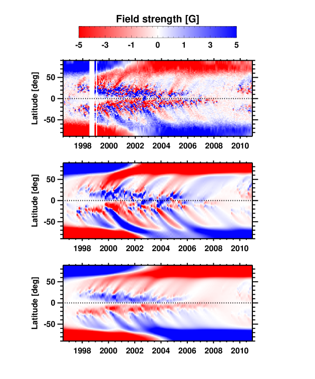
Figure 1: Time-latitude diagrams of the longitudinally averaged radial magnetic field at the solar surface. Top panel: observation (SoHO/MDI synoptic magnetic field data); middle panel: simulation using the actual tilt angles of bipolar magnetic regions; bottom panel: simulation using tilt angles according to a fitted latitude dependence.

Fig. 1 shows observed and simulated time-latitude diagrams of the longitudinally averaged radial surface field. Although there are differences in detail, the simulation on the basis of the actual individual tilt angles (middle panel) reproduce the main features of the evolution of the surface field rather well. Deviations in detail can be traced back to a small number of errors in the tilt data of Li & Ulrich (2012). We have confirmed that these errors do not significantly affect the polar fields and dipole moment around the activity minimum, for which only the cross-equator transport of magnetic flux from low-latitude active regions is important (Jiang et al., 2014a). To avoid potential bias, we therefore chose not to correct these errors, which would have improved the agreement of the time-latitude diagrams.

The main difference between the simulation with actual tilt angles and that with Joy’s law becomes apparent when considering the axial dipole moment of the Sun,

$$D(t)=\frac{3}{2}\int_{\pi/2}^{-\pi/2}\left\langle B(\lambda,t)\right\rangle\cos\lambda\sin\lambda\,d\lambda,$$ (2)

where $\langle B(\lambda,t)\rangle$ is the longitudinally averaged radial surface field. The axial dipole moment is a better suited quantity than the polar field for the comparison of observation and simulation. It is uniquely defined and limits the effect of asymmetries in the magnetic flux distribution on the two hemispheres (such as non-synchronous reversals of the polar fields). Around activity minima, the axial dipole moment is dominated by the polar fields and represents the relevant quantity for the poloidal magnetic flux connected to the polar fields. Likewise, it also represents the open heliospheric magnetic flux during these periods.

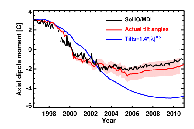
Figure 2: Time evolution of the solar axial dipole moment. The curves correspond, respectively, to observed SoHO/MDI magnetic maps (black), a simulation using the actual tilt angles of bipolar magnetic regions (red), and a simulation using tilt angles according to a fitted latitude dependence (blue).

Fig. 2 shows the evolution of the axial dipole moment as determined from observations (SoHO/MDI magnetic maps) and our SFT simulations. The simulation based on the actual tilt angles follows the observed evolution of the axial dipole moment well within the shaded error range (see below). On the other hand, employing Joy’s law for the tilt angles leads to a much too strong axial dipole moment in the declining and minimum phases of cycle 23. This behavior is typical for previous attempts to reproduce the observed weak axial dipole moment and polar field by SFT simulations, unless the models were arbitrarily modified (e.g., in terms of meridional flow variations).

We estimate the error of the axial dipole moment in our simulations as follows. The main source of uncertainty are the errors in the determination of the tilt angles. We have therefore used a different data source, the Kitt Peak Synoptic Magnetograms, to independently redetermine the tilt angles of about 30% of the bipolar regions considered by Li & Ulrich (2012), who used SoHO/MDI magnetograms. The regions were chosen from the SOON list, their area determined by applying a threshold on measured magnetic flux density, and their tilt then calculated using the line connecting the centers of gravity of the positive and negative polarity parts. Comparison with the data of Li & Ulrich (2012) yields an overall value of $\sigma=11.5^{\circ}\,$ for the rms scatter. However, the error is dependent on the area of the region; e.g., for the 50 biggest ARs, the scatter is reduced to about $5^{\circ}$. The dependence on area, $A$ (in microhemispheres), can be roughly approximated by the function

$$\sigma(A)=\left\{\begin{array}[]{l l}18^{\circ}-0.02A&\textrm{for}A<650.\\ 5^{\circ}&\textrm{otherwise}.\end{array}\right.$$ (3)

We carried out 20 SFT simulations with random scatter of the AR tilts according to this function. The rms variation of the resulting axial dipole strength is then taken as error estimate.

3 Origin of the low dipole moment

Figure 3 illustrates the reason for the discrepancy between the simulation with actual tilt angles and the one based upon Joy’s law. Shown are cumulative contributions of magnetic regions to the change of the dipole moment (since 1996) as a function of emergence latitude (modulus). The individual contribution of a magnetic region for large times is proportional to $\Delta=A^{3/2}\,\sin(\alpha)\exp(-\lambda^{2}/110)$, where $A$ is the area of the region (Jiang et al., 2014a). The normalized cumulated contributions using the actual tilt angles (dashed curve) closely follow those when assuming Joy’s law (solid curve) for emergence latitudes poleward of $\pm 10^{\circ}$ from the equator. Nearer to the equator, the curves diverge: the actual tilt angles of magnetic regions emerging in this range statistically deviate strongly from Joy’s law in such a way that the resulting total change of the dipole moment since 1996 is reduced by about 40%. The is mainly due to comparatively few regions in the (positive and negative) tails of the distribution of $\Delta$, i.e., a result of random variations together with low-number statistics.

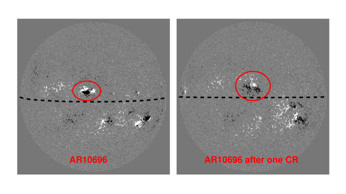
Figure 4: Example of a bipolar magnetic region that significantly weakened the axial dipole moment in the declining phase of cycle 23. Shown are SoHO/MDI magnetic maps of the active region AR10696 taken Nov 5, 2004 (left panel) and Dec 2, 2004 (right panel, after one solar rotation, then denominated AR10708), respectively. Positive magnetic flux is indicated in white, negative flux in black. Owing to its near-equator emergence, high tilt, and abnormal polarity orientation in the North/South direction, the region provides a significant amount of negative flux that is transported over the equator (by supergranular random walk) to the southern hemisphere. Through poleward advection (mainly by meridional flow) this flux eventually weakened the buildup of positive flux around the south pole of the Sun, thus lowering the axial dipole moment.

An example for a big magnetic region with ‘wrong’ orientation (i.e., opposite to the majority of the magnetic regions during this cycle) of the magnetic polarities in the North-South direction is active region AR10696, which appeared in November 2004. Magnetic maps for this region are shown in Fig. 4. Since it emerged near the equator, a significant amount of negative-polarity magnetic flux could cross the equator and thus significantly reduce the buildup of the axial dipole moment in the descending phase of the cycle (Cameron et al., 2013). Since the magnetic flux at the poles around activity minima is typically of the order of the flux of only one big bipolar magnetic region, a few bipolar regions emerging near the equator can have a significant impact.

4 Comparison with cycles 21 and 22

While Joy’s law was a reasonable assumption in SFT simulations before cycle 23, we have seen that it is inadequate to describe the evolution of the axial dipole moment in cycle 23. It is therefore of interest to consider a similar analysis as the one resulting in Fig. 3 for earlier cycles. Since magnetic information is necessary to properly determine the tilt angle (particularly for the big regions with ‘wrong’ tilt), we have to restrict ourselves to cycles 21 and 22, for which Kitt Peak National Observatory (KPNO) synoptic magnetograms are available. Since these are based on observations along the central meridian only, they contain not all of the emerging bipolar regions detectable by full-disk magnetograms such as those from SoHO/MDI, but still provide a statistically meaningful sample. We used the synoptic magnetograms to determine the individual tilt angles of bipolar regions emerging in cycles 21-23. The (normalized) cumulative distributions to the change of the dipole moment during these cycles are given in Figure 5. For comparison, the result for cycle 23 on the basis of tilts from the MDI magnetograms (Fig. 3) is also reproduced. The two results for cycle 23 (from MDI and KPNO data, respectively) are consistent with each other (taking into account that the KPNO analysis covers only 30% of the MDI regions): both show the big deviation from Joy’s law for latitudes below $10^{\circ}$. On the other hand, the result for cycle 21 and 22 (combined in order to improve statistics) is fully consistent with tilt angles according to Joy’s law. This indicates these cycles were less strongly affected than cycle 23 by randomness concerning the tilt angles of low-latitude active regions in the descending phase of the cycle.

5 Concluding remarks

Our SFT simulations have shown that the weak axial dipole moment (weak polar fields) around the activity minimum of cycle 23 are a result of a number of low-latitude bigger active regions whose ‘wrong’ tilt angles did not follow Joy’s law. Since the poloidal magnetic flux related to the axial dipole moment (directly related to the polar fields) is the dominant source of the toroidal flux that emerges in the subsequent cycle (Cameron & Schüssler, 2015), its low amplitude during the declining phase of cycle 23 caused the weakness of the current cycle 24. The dependence on the properties of big bipolar regions emerging in the vicinity of the solar equator, which are affected by randomness, strongly limits the scope of predicting solar cycle strength: until the amplitude of the polar fields is established around solar minimum, no sensible prediction of the strength of the next cycle can be made. Sound predictions projecting even further into the future are virtually impossible.

Table 1: List of the recurrent ARs. At Time (yyyymmdd), the ARs reached their maximum area (in microhemispheres). The column AR gives the active regions that are retained in the SFT simulations.

No.	Recurrent AR	AR	Time	Latitude	Area	Tilt
1	8375	8398	19981109	21.0	964	48.13
2	8771	8739	19991125	-15.0	1097	3.63
3	8759	8731	19991109	10.0	1230	1.54
4	9085	9046	20000720	15.0	405	29.88
5	9131	9090	20000825	15.0	312	38.84
6	9636	9601	20010926	14.0	538	36.56
7	9670	9628	20011019	-18.0	711	16.66
8	9672	9704	20011026	-18.0	791	44.88
9	9684	9715	20011104	5.0	737	16.04
10	9751	9715	20011226	4.0	671	15.86
11	9973	9934	20020529	-16.0	1283	8.43
12	10036	10069	20020721	-6.0	1429	17.57
13	10105	10069	20020910	-8.0	2028	28.38
14	10386	10365	20030617	-7.0	418	54.31
15	10464	10484	20030926	4.0	817	17.88
16	10507	10488	20031119	10.0	1190	13.23
17	10508	10486	20031119	-17.0	937	25.08
18	10520	10484	20031216	1.0	232	56.46
19	10661	10652	20040818	10.0	724	24.04
20	10708	10696	20041203	8.0	219	55.61
21	10743	10735	20050319	-8.0	525	40.70
22	10750	10735	20050408	-7.0	205	51.75
23	10775	10792	20050612	10.0	485	31.27
24	10803	10792	20050825	12.0	272	40.14
25	10875	10865	20060425	-10.0	644	32.90
26	10904	10908	20060812	-13.0	1003	9.94
27	10930	10923	20061212	-6.0	910	29.36
28	10935	10923	20070104	-6.0	365	41.59

Figure 3: Cumulative contributions (in latitudinal distance from the equator) of magnetic regions to the change of the axial dipole moment since 1996. Results are given assuming tilt angles according to Joy’s law ($\propto 1.4\sqrt{|\lambda|}$, solid curve) and for the actual individual tilt angles (dashed curve).

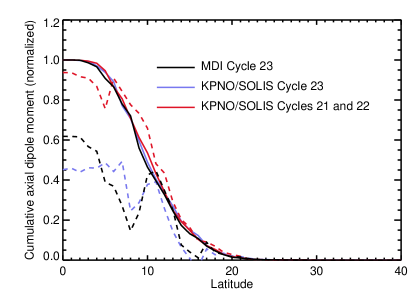
Figure 5: Cumulative contributions (in latitudinal distance from the equator) of magnetic regions to the change of the axial dipole moment during cycles 21, 22, and 23. Full lines give the result assuming tilt angles according to Joy’s law (almost coincident with each other), dashed lines for the case using the actual individual tilt angles. The black curves are reproduced from Fig. 3 (on the basis of MDI full-disk magnetograms), blue lines indicates results from KPNO synoptic magnetograms for cycle 23, and red lines the corresponding results for cycles 21 and 22 combined.

References

- Baumann et al. (2004) Baumann, I., Schmitt, D., Schüssler, M., & Solanki, S. K. 2004, A&A, 426, 1075
- Cameron et al. (2013) Cameron, R. H., Dasi-Espuig, M., Jiang, J., Işık, E., Schmitt, D., & Schüssler, M. 2013, A&A, 557, A141
- Cameron et al. (2010) Cameron, R. H., Jiang, J., Schmitt, D., & Schüssler, M. 2010, ApJ, 719, 264
- Cameron & Schüssler (2010) Cameron, R. H. & Schüssler, M. 2010, ApJ, 720, 1030
- Cameron & Schüssler (2015) —. 2015, Science, 347, 1333
- Gizon et al. (2010) Gizon, L., Birch, A. C., & Spruit, H. C. 2010, ARA&A, 48, 289
- González Hernández et al. (2008) González Hernández, I., Kholikov, S., Hill, F., Howe, R., & Komm, R. 2008, Sol. Phys., 252, 235
- Hathaway (2010) Hathaway, D. H. 2010, Living Reviews in Solar Physics, 7, 1
- Hathaway & Rightmire (2010) Hathaway, D. H. & Rightmire, L. 2010, Science, 327, 1350
- Hathaway & Rightmire (2011) Hathaway, D. H. & Rightmire, L. 2011, ApJ, 729, 80
- Jiang et al. (2013) Jiang, J., Cameron, R. H., Schmitt, D., & Schüssler, M. 2013, Space Sci. Rev., 176, 289
- Jiang et al. (2014a) Jiang, J., Cameron, R. H., & Schüssler, M. 2014a, ApJ, 791, 5
- Jiang et al. (2014b) Jiang, J., Hathaway, D. H., Cameron, R. H., Solanki, S. K., Gizon, L., & Upton, L. 2014b, Space Sci. Rev.
- Jiang et al. (2010) Jiang, J., Işik, E., Cameron, R. H., Schmitt, D., & Schüssler, M. 2010, ApJ, 717, 597
- Leighton (1964) Leighton, R. B. 1964, ApJ, 140, 1547
- Li & Ulrich (2012) Li, J. & Ulrich, R. K. 2012, ApJ, 758, 115
- Mackay & Yeates (2012) Mackay, D. & Yeates, A. 2012, Living Reviews in Solar Physics, 9, 6
- Muñoz-Jaramillo et al. (2012) Muñoz-Jaramillo, A., Sheeley, N. R., Zhang, J., & DeLuca, E. E. 2012, ApJ, 753, 146
- Nandy et al. (2011) Nandy, D., Muñoz-Jaramillo, A., & Martens, P. C. H. 2011, Nature, 471, 80
- Owens & Forsyth (2013) Owens, M. J. & Forsyth, R. J. 2013, Living Reviews in Solar Physics, 10, 5
- Russell et al. (2010) Russell, C. T., Luhmann, J. G., & Jian, L. K. 2010, Reviews of Geophysics, 48, 2004
- Scherrer et al. (1995) Scherrer, P. H., Bogart, R. S., Bush, R. I., Hoeksema, J. T., Kosovichev, A. G., Schou, J., Rosenberg, W., Springer, L., Tarbell, T. D., Title, A., Wolfson, C. J., Zayer, I., & MDI Engineering Team. 1995, Sol. Phys., 162, 129
- Schrijver & Liu (2008) Schrijver, C. J. & Liu, Y. 2008, Sol. Phys., 252, 19
- Sheeley (2005) Sheeley, Jr., N. R. 2005, Living Reviews in Solar Physics, 2, 5
- Smith & Balogh (2008) Smith, E. J. & Balogh, A. 2008, Geophys. Res. Lett., 35, 22103
- Snodgrass (1983) Snodgrass, H. B. 1983, ApJ, 270, 288
- Stenflo & Kosovichev (2012) Stenflo, J. O. & Kosovichev, A. G. 2012, ApJ, 745, 129
- Sun et al. (2011) Sun, X., Liu, Y., Hoeksema, J. T., Hayashi, K., & Zhao, X. 2011, Sol. Phys., 270, 9
- Upton & Hathaway (2014a) Upton, L. & Hathaway, D. H. 2014a, ApJ, 792, 142
- Upton & Hathaway (2014b) —. 2014b, ApJ, 780, 5
- van Ballegooijen et al. (1998) van Ballegooijen, A. A., Cartledge, N. P., & Priest, E. R. 1998, ApJ, 501, 866
- Wang et al. (2015) Wang, Y.-M., Colaninno, R. C., Baranyi, T., & Li, J. 2015, ApJ, 798, 50
- Wang et al. (1989) Wang, Y.-M., Nash, A. G., & Sheeley, Jr., N. R. 1989, Science, 245, 712
- Wang & Sheeley (2009) Wang, Y.-M. & Sheeley, N. R. 2009, ApJ, 694, L11
- Yeates (2014) Yeates, A. R. 2014, Sol. Phys., 289, 631