Rogue Active Regions and the Inherent Unpredictability of the Solar Dynamo

Abstract

New developments in surface flux transport modeling and theory of flux transport dynamos have given rise to the notion that certain large active regions with anomalous properties (location, tilt angle and/or Hale/non-Hale character) may have a major impact on the course of solar activity in subsequent years, impacting also on the amplitude of the following solar cycles. Here we discuss our current understanding of the role of such “rogue” active regions in cycle-to-cycle variations of solar activity.

1 Dynamo-based cycle forecasting and rogue active regions

In the last ten years significant advance has been made towards solar cycle forecasting based on dynamo models. Most efforts in this direction are based on the flux transport dynamo concept. An essential feature of these models is that the poloidal magnetic field, peaking near the poles around the minimum of the solar cycle, serves as seed for the toroidal field built up in the next cycle: the strength of the polar field is therefore a good predictor of the amplitude of the next solar cycle. This is confirmed by a good empirical correlation between the respective indicators (e.g. Muñoz-Jaramillo et al. 2013). The problem of predicting an upcoming solar cycle is then reduced to the problem of predicting the peak strength of the polar field being built up during the course of the ongoing cycle. Surface flux transport models based on observations indicate that the polar magnetic flux is built up from the unbalanced trailing polarity flux originating in active regions of the ongoing cycle. As the leading and trailing fluxes in a bipolar magnetic region are initially balanced, a significant contribution to the polar flux is only expected if the two polarities are located at significantly different latitudes, facilitating a more effective cancellation of flux of one (typically, leading) polarity with its opposite hemisphere counterpart across the equator. This is, in turn, easier to achieve at low latitudes and for relatively high tilts.

A single bipolar magnetic region represents a contribution

$$\delta D_{\mathrm{BMR}}\approx F\,d\,\sin\alpha\,\sin\theta$$ (1)

to the solar axial dipole moment where $F$ is magnetic flux, $d$ is the separation of the two polarities, $\alpha$ is the tilt angle, $\theta$ is the colatitude. Active regions with unusually high or deviant values of the parameters may then be expected to induce significant fluctuations in the strength of the polar magnetic field built up in a cycle. In addition to tilt quenching, i.e. a nonlinear dependence of the mean value of the tilt angle $\alpha$ on cycle amplitude (Dasi-Espuig et al. 2010), a possibly important factor in intercycle variations are fluctuations in the unbalanced flux contribution by active regions, related to the random nature of the flux emergence process. Indeed, while Cameron et al. (2010) find that tilt quenching satisactorily reproduces the observed polar field amplitude built up during cycles 15 to 22, the same approach fails for Cycle 23. Cameron et al. (2013) suggested that the vagaries of the flux emergence process can be responsible for such deviations from the expected behaviour of the solar cycle. This was corroborated by Jiang et al. (2014, 2015) who showed that assimilating individual active regions into the model, the polar field amplitude built up in Cycle 23 can be reproduced.

This suggests that in extreme cases even a single large active region with unusual properties can have a dramatic impact on the further course of cyclic solar magnetic activity. To have such a major impact, an active region needs to be (1) large, (2) unusually tilted, strongly deviating from Joy’s law (e.g. non-Joy or very “over-Joy”) (3) positioned at low latitudes to facilitate the cross-equatorial cancellation of flux of one polarity. In a recent work (Nagy et al. 2017) we reported examples of potentially dramatic effects of such “rogue” active regions on the solar cycle in a dynamo model. The main results from this research are summarized in the next section, while the third, concluding section briefly discusses the implications of these results for the importance of long-term datasets.

2 Rogue active regions in the $2\times 2$D dynamo

Dynamo models incorporating individual active regions have been developed by several research groups (Yeates and Muñoz-Jaramillo 2013, Yeates et al. 2015, Miesch and Teweldebirhan 2016, Hazra et al. 2017). One particularly attractive approach is the $2\times 2$D dynamo developed in Montreal (Lemerle et al. 2015, Lemerle and Charbonneau 2017).

The model couples a 2D surface flux transport simulation (SFT) with a 2D axisymmetric flux transport dynamo (FTD). The azimuthally averaged SFT component provides the upper boundary condition for the FTD component, while the FTD module couples toward the SFT by the emergences of new bipolar magnetic regions (BMR). This step is based on a semi-empirical emergence function that gives the emergence probability of a BMR depending on the toroidal magnetic field $B_{\phi}$ at the bottom of the convective zone in the FTD module. In the optimized solution used here the emergence probability is proportional to $B_{\phi}^{3/2}$; there is, however, a threshold below which flux emergence is suppressed. Properties of the emerging BMR — flux, angular separation, tilt — are randomly drawn from distribution functions for these quantities built from observed statistics of solar active region emergences (see Appendix A in Lemerle et al. 2015).

The other nonlinearity built in the model is tilt quenching: a reduction of the average BMR tilt angle $\alpha$ with $B_{\phi}$ according to the ad hoc formula

$$\alpha=\frac{\alpha_{0}}{1+(B_{\phi}/B_{q})^{2}},$$ (2)

where $B_{q}$ is the quenching field amplitude.

The main advantages of this model are its high numerical efficiency and the fact that it is calibrated to follow accurately the statistical properties of the real Sun. The complete latitude–longitude representation of the simulated solar surface in the SFT component further makes it possible to achieve high spatial resolution and account for the effect of individual active region emergences.

The reference solar cycle solution presented in Lemerle and Charbonneau (2017), which is adopted in the numerical experiments of Nagy et al. (2017) is defined by 11 adjustable parameters, which were optimized using a genetic algorithm designed to minimize the differences between the spatiotemporal distribution of emergences produced by the model, and the observed sunspot butterfly diagram. Thanks to the numerical efficiency of the model, the reference solution can be run for many hundreds of cycles, in contrast to the limited number of actual solar cycles observed. We have studied this reference solution looking for sudden changes in the behaviour of the dynamo and trying to identify the culprits. We found that in some cases even a single rogue BMR can have a major effect on the further development of solar activity cycles, boosting or suppressing the amplitude of subsequent cycles. In extreme cases an individual BMR can completely halt the dynamo, causing a grand minimum. Alternatively a dynamo on the verge of being halted can also be resuscitated by a rogue BMR with favourable characteristics. Rogue BMR also have the potential to induce significant hemispheric asymmetries in the solar cycle.

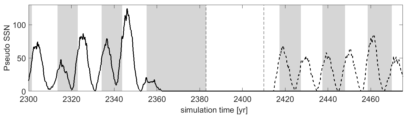
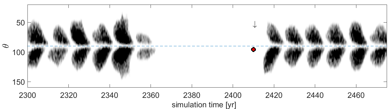
Figure 1: A rogue sunspot restarting cyclic activity after a 60 years long grand minimum state. On the top panel black dashed line shows the cycles launched by a single BMR manually inserted on the souther hemisphere, close to the equator. The gray background corresponds to the negative dipole periods, while the vertical dashed lines show the 30 years long period, when it was zero. On the bottom panel we show the butterfly diagram of the simulation run with the BMR inserted. The position of the leading polarity is indicated by the red dot. The properties of this BMR are listed in the first row of Table 1.

In addition to these effects, discussed in detail in Nagy et al. (2017), here we present a further possible role of rogue active regions. While, owing to the presence of the field strength threshold, the dynamo is not self-excited and it can never recover from a grand minimum state, in one case, displayed in Figure 1, we manually insert a large rogue BMR in the model at $t=2410$ during a grand minimum phase, overriding the threshold. A strong “over-Joy” BMR with similar properties (given in the first data row of Table 1) did indeed arise in one of the model runs (see Figure 4 of Nagy et al. 2017). As apparent from the figure, this BMR is capable of inducing a recovery even from a long lasting deep grand minimum state.

Figure 2 summarizes the results of several numerical experiments that aimed to study how the characteristics of active regions affect the subsequent, or even the ongoing cycle (Nagy et al., 2017). For this analysis a ’test’ BMR was selected with characteristics listed in the second data row of Table 1. (Such a BMR did also emerge spontaneously during the reference simulation run.) This active region was manually inserted into ongoing simulations with preset parameters. The experiments were performed for three cycles of average, below average and above average, respectively. In each case two series of experiments were carried out with Hale (anti-Hale) test-BMR in order to increase (decrease) the dipole moment of the examined cycle. The characteristics of the test-BMR – emergence time and latitude, flux, tilt angle and angular separation – were changed one by one in order to map the impact of each property on the subsequent simulated cycle.

As it is shown in Figure 2, the flux, tilt angle and separation (green, blue and magenta curves) have quite similar effect on the temporal evolution of the dipole moment, and consequently of the next cycle. The good agreement of the green, blue and magenta curves in the plot confirms that the effect of these factors can indeed be combined in the form given in equation (1) providing a good measure of the “dynamo efficiency” of individual active regions at a given latitude.

The red curve, showing the influence of the emergence latitude, indicates that the effect of a BMR decreases with the emergence latitude. Nevertheless, BMRs appearing $20^{\circ}$ far from the equator can still have significant impact on the next cycle in the present model (but see discussion in the following section).

By setting the emergence time Nagy et al. (2017) found that active regions emerging during the rising phase of the cycle can modify even the ongoing cycle, but this effect disappears at cycle maximum. The strongest impact on the subsequent cycle is obtained if the test BMR emerges at cycle maximum while for later epochs the effect gradually subsides.

$\theta_{\mathrm{lead}}$	$\theta_{\mathrm{trail}}$	$F$ [$10^{23}$ Mx]	$\alpha$	$d$	$\delta D_{\mathrm{BMR}}$[$10^{23}$ Mx]	J/H
95.6∘	104.1∘	–3.58	$-15.53^{\circ}$	32.11∘	0.5293	J/H	Figure 1
89.5∘	82.1∘	–1.39	13.98∘	30.97∘	–0.1810	J/H, J/a-H	Figure 2

Table 1: Parameters of active regions discussed in the paper. Colatitudes $\theta_{\mathrm{lead}}$ and $\theta_{\mathrm{trail}}$ are the latitudinal positions of leading and trailing polarities; $F$ is the flux of the trailing polarity ($F_{\mathrm{trail}}=-F_{\mathrm{lead}}$); $\alpha$ is the tilt angle and $d$ is the angular separation of leading and trailing polarities. $\delta D_{\mathrm{BMR}}$, the contribution of the BMR to the global dipole moment, is defined according to Equation 1. J/H indicates whether the active region is (anti-)Joy/(anti-)Hale. In the case of the second row a J/H (J/a-H) test-BMR increases (decreases) the dipole moment during the experiments detailed in Section 5 of (Nagy et al., 2017).

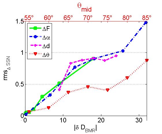
Figure 2: Average effect of varying the properties of a BMR (2nd data row of Table 1), inserted in the simulations at cycle maximum, on the amplitude of the subsequent cycle. Variations in BMR flux (green), tilt angle (blue) and polarity separation (magenta) are converted to the contribution to the dipole moment (in units of $10^{21}\,$Mx) according to Equation 1, while the varying colatitudes (red) are shown on the top axis.

3 Implications for observational records and their analysis

It is to be noted that the magnetic fluxes of the rogue BMR identified in the simulations are mostly within or only slightly outside the size range of solar active regions on record. While for historical records the magnetic fluxes can only be roughly estimated based on sunspot areas, such estimates suggest that the largest spots on record were in the $(1$–$3.5)\cdot 10^{23}\,$Mx range. What seems to be more exaggerated is the polarity separations: in fact, observed values of $d$ do not normally exceed about $20^{\circ}$. The high values in the simulations are due to the fact that Lemerle et al. (2015) calibrate their $d$–$F$ relation to cycle 21 which did not show any AR with flux exceeding $10^{23}\,$Mx, so the application to rogue spots is based on a somewhat dubious extrapolation. Nevertheless, equation (1) indicates that a 33 % reduction in $d$ is readily compensated by, e.g. a 50 % increase in $F$ which is still not inconceivable. So while the occurrence rate of rogue AR might be overestimated in the model, the reality of the phenomenon is not brought into question.

In the CESAR Solar Data Archives maintained by Kanzelhöhe Observatory a list of the largest sunspots recorded in the observatory is presented. It is remarkable that 5 out of the 6 largest spots on the list arose in the period 1946–1951, i.e. during the declining phase of Cycle 18. It is well known that Cycle 19 that followed this was by far the strongest and most anomalous cycle on record; reproducing its amplitude represents a challenge for dynamo based cycle prediction methods.

A detailed analysis of the effect of these and similar large active regions on the dynamo is, however, still hindered by a number of unresolved issues both from the theoretical and observational side.

On the theoretical side, equation (1) only gives the initial contribution of a BMR to the global dipole. The final net contribution will be determined by the amount of unbalanced flux, i.e. by the amount of flux cancelling across the equator during the subsequent evolution of the BMR. The relation between initial and final contributions has been studied by Jiang et al. (2014); however, this relation may be quite sensitive to model details, possibly explaining why the latitude dependence reported by Nagy et al. (2017) differs. This dependence on model details is currently under study; a more reliable measure of the latitude dependence of the dynamo efficiency of active regions can only be constructed after the clarification of this issue.

From the observational point of view, detailed and reliable information on the evolution of large active regions (rogue active region candidates) is needed. In currently available historical records even the reported sunspot areas often differ by a large amount between various sources. Magnetic flux and even magnetic polarity data are not always well correlated with the white light information on sunspot groups and they are only sporadically available for epochs prior to the invention of magnetographs. Collecting and correlating all relevant information from all available sources is therefore important for a reliable assessment of the dynamo effectivity of large active regions and for identifying rogue active region candidates.

Finally, the largest active regions often live for several Carrington rotations, displaying dramatic changes in extent, appearance and spot distribution. During this extended period of time the constituent sunspots only gradually decay to release weak magnetic flux into the plage where the linear transport processes modelled in SFT simulations will take over. Representing active regions as a simple bipolar pair of instantaneous point sources is clearly a very crude approximation to this process. More realistic models of active region sources of magnetic flux in SFT simulations need to be developed, and for these every piece of information concerning the detailed structure and evolution of large active regions can potentially have a high significance.

As a final remark we note that unusually large active regions harbouring a significant amount of free energy may also be responsible for superflares, as recently discussed by Shibata et al. (2013), Maehara et al. (2017) or Namekata et al. (2017). As tilt and free energy are closely related to the writhe and twist of magnetic flux bundles, respectively, which are but two manifestations of magnetic helicity, the categories of rogue AR and superflaring AR may overlap to a significant extent. Yet we stress that size alone does not imply that an active region will have a major influence: it is the added presence of helicity, manifest as tilt and/or free energy, that can lead to a major effect of sunspots on either space weather or space climate.

References

- Cameron et al. (2013) Cameron, R. H., Dasi-Espuig, M., Jiang, J., Işık, E., Schmitt, D., and Schüssler, M.: 2013, A&A 557, A141
- Cameron et al. (2010) Cameron, R. H., Jiang, J., Schmitt, D., and Schüssler, M.: 2010, ApJ 719, 264
- Dasi-Espuig et al. (2010) Dasi-Espuig, M., Solanki, S. K., Krivova, N. A., Cameron, R., and Peñuela, T.: 2010, A&A 518
- Hazra et al. (2017) Hazra, G., Choudhuri, A. R., and Miesch, M. S.: 2017, ApJ 835, 39
- Jiang et al. (2014) Jiang, J., Cameron, R. H., and Schüssler, M.: 2014, ApJ 791, 5
- Jiang et al. (2015) Jiang, J., Cameron, R. H., and Schüssler, M.: 2015, ApJ 808, L28
- Lemerle and Charbonneau (2017) Lemerle, A. and Charbonneau, P.: 2017, ApJ 834, 133
- Lemerle et al. (2015) Lemerle, A., Charbonneau, P., and Carignan-Dugas, A.: 2015, ApJ 810, 78
- Maehara et al. (2017) Maehara, H., Notsu, Y., Notsu, S., Namekata, K., Honda, S., Ishii, T. T., Nogami, D., and Shibata, K.: 2017, PASJ 69, 41
- Miesch and Teweldebirhan (2016) Miesch, M. S. and Teweldebirhan, K.: 2016, Advances in Space Research 58, 1571
- Muñoz-Jaramillo et al. (2013) Muñoz-Jaramillo, A., Balmaceda, L. A., and DeLuca, E. E.: 2013, Physical Review Letters 111, 041106
- Nagy et al. (2017) Nagy, M., Lemerle, A., Labonville, F., Petrovay, K., and Charbonneau, P.: 2017, Sol. Phys. 292, 167
- Namekata et al. (2017) Namekata, K., Sakaue, T., Watanabe, K., Asai, A., Maehara, H., Notsu, Y., Notsu, S., Honda, S., Ishii, T. T., Ikuta, K., Nogami, D., and Shibata, K.: 2017, ApJ 851, 91
- Shibata et al. (2013) Shibata, K., Isobe, H., Hillier, A., Choudhuri, A. R., Maehara, H., Ishii, T. T., Shibayama, T., Notsu, S., Notsu, Y., Nagao, T., Honda, S., and Nogami, D.: 2013, PASJ 65, 49
- Yeates et al. (2015) Yeates, A. R., Baker, D., and van Driel-Gesztelyi, L.: 2015, Sol. Phys. 290, 3189
- Yeates and Muñoz-Jaramillo (2013) Yeates, A. R. and Muñoz-Jaramillo, A.: 2013, MNRAS 436, 3366