Sunspot group tilt angles from drawings for cycles 19-24

Abstract

The tilt angle of a sunspot group is a critical quantity in the surface transport of magnetic flux and the solar dynamo. To contribute long-term databases of the tilt angle, we developed an IDL routine, which allows the user to interactively select and measure sunspot positions and areas on the solar disc. We measured the tilt angles of sunspot groups for solar cycles 19-24 (1954.6-2017.8), using the sunspot drawing database of Kandilli Observatory. The method is similar to that used in the discontinued Mt. Wilson and Kodaikanal databases, with the exception that sunspot groups were identified manually, which has improved the accuracy of the resulting tilt angles. We obtained cycle averages of the tilt angle and compared them with the values from other datasets, keeping the same group selection criteria. We conclude that the previously reported anti-correlation with the cycle strength needs further investigation.

1 Introduction

The angle between the line joining opposite polarities and the local latitude is called the tilt angle of a sunspot group. It is defined as positive when the preceding polarity is closer to the equator. This is an important quantity because, through latitudinal separation between opposite polarities of bipolar regions, it controls the net magnetic flux which contributes to the global axial dipole moment of the Sun, which is well-correlated with the strength of the subsequent activity cycle. Systematic changes in the tilt angle by inflows at the surface [(Jiang et al. 2010)] or by stabilisation of deep-seated flux tubes [(Işık 2015)] can play important roles in the nonlinear saturation of the solar dynamo.

It is evident from the literature that long-term tilt angle databases should be enriched, to evaluate the relationship of its cycle averages with amplitude fluctuations of solar cycles. Our main motivation to construct an additional dataset is to make an independent test of the reported anti-correlation between cycle-averaged tilt angle and the cycle strength [(Dasi-Espuig et al. 2010)].

(a)

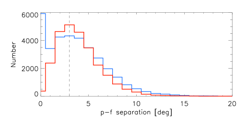
(b)

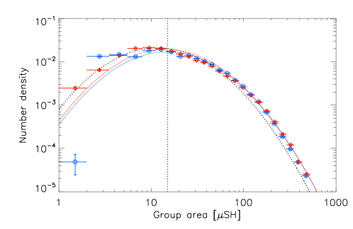
Figure 1: Distributions for (a) the angular separation between p- and f- parts, and (b) the group area for $S>3^{\circ}$, the vertical line in panel (a), normalised to the number of groups with $A>1$ MSH (Kandilli in red, DPD in blue). The vertical error bars show the standard deviation of the mean, and the horizontal bars show the area bins. Lognormal fits were made for $A>15~{}\mu$SH, and a model function from [Baumann & Solanki (2005)] is also shown (dotted curve).

2 Measuring sunspot groups

We used the digitised web archive of Kandilli Observatory sunspot drawings, which have been systematically produced since 1944, using a 20-cm equatorial-mount refractor with 307-cm focal length. We developed and used an interactive IDL routine, to record the positions and areas of umbral features, including pores, so far as they were detected and drawn by the observers. The selection of pixels is based on a region-of-interest algorithm. We also measured the inclination of the solar axis relative to the local meridian, at the time of each observation. This is used not only to determine the position angle of each spot, but also to correct for the small tilt of the scanned drawing, by referring to the exact value of the inclination. To measure the tilt angle, we use the method of [Howard (1991)], with the exception that we adopt group identifications of the observers, rather than using an automated algorithm. There are 1-2 year data gaps in parts of cycle 19 (1955-57 and 1962-63) and in cycle 22 (1993).

Figure 1a shows the histogram of the angular separation, $S$, between the preceding (p-) and follower (f-) parts of our groups with area $A>1~{}\mu$SH (micro solar hemisphere) and distance to disc centre, $\rho<60^{\circ}$. For comparison, we plotted the Debrecen Photoheliographic Record (DPD) results [(Baranyi et al. 2016)] keeping the same criteria. Since DPD provides the angular distance to the central meridian (CMD), we took CMD$<60^{\circ}$. For DPD, we chose only those group measurements which have a measured tilt angle. A local peak around $3^{\circ}$ is present in both datasets. In our data, the distribution drops rather sharply towards more compact groups, owing to the tendency of observers not to classify them as bipolar (we measured only ‘bipolar’ regions, excluding McIntosh types A and H). In DPD data, however, there is an additional peak at the smallest separations (see also [(Baranyi 2015), Baranyi 2015], Fig. 3). To have a reliable comparison of tilt angles in these datasets, we considered only groups with $S>3^{\circ}$, as also suggested by [(Baranyi 2015), Baranyi (2015)] and [Senthamizh Pavai et al. (2015)], in addition to the criteria described for Fig. 1a. The discrete area distributions for both datasets are shown in Fig. 1b, along with lognormal function fits, which are applied to data above a group area of $15$ MSH. We adopted this threshold from [Baumann & Solanki (2005)], whose model distribution including lognormal spot decay rates is also shown for comparison. Our data fits well with the DPD in terms of the group area distribution, except for very small areas of a few $\mu$SH, for which intrinsic uncertainties become comparable with the group area in any case.

3 Joy’s law and cycle-averaged tilt angles

Figure 2 shows the latitude dependence of the tilt angle of Kandilli data, for different hemispheres and for unsigned latitude. We applied here the same group selection criteria as in Fig. 1b. We confirm [(Baranyi 2015), Baranyi’s (2015)] result that there is a persistent pattern in the latitudinal dependence of the tilt angle. In particular, there is a significant north-south asymmetry in Joy’s law for our six-cycle averages, and a double-hump pattern in the global averages of $\alpha(|\lambda|)$, all very similar to those found for three cycles by [(Baranyi 2015), Baranyi (2015, Figs. 8-9)]. A linear least-squares fit gives a Joy’s law slope of $0.398\pm 0.006$, where the y-intercept is forced to zero. When the fit is confined to $|\lambda|<30^{\circ}$ we find $0.405\pm 0.007$, which is closer to that found by [(Baranyi 2015), Baranyi (2015)]. When the intercept is not forced, we find $\alpha=(0.328\pm 0.015)\lambda+(1.34\pm 0.27)$.

Figure 2: Joy’s law for signed (left panel) and unsigned (right panel) latitude. The error bars show standard deviation of the means over $5^{\circ}$ bins.

We calculated cycle-averages of the tilt angles $\langle\alpha\rangle$ and latitudes $\langle\lambda\rangle$, of all groups with the same criteria as in Fig. 1b to check for a systematic dependence on cycle strength. Figure 3 shows the ratio $\langle\alpha\rangle/\langle\lambda\rangle$ for Kandilli and DPD. It is known that unipolar and compact groups have an almost zero mean tilt angle, whereas ephemeral regions have negative mean tilt angles in magnetographic results [(Tlatov et al. 2013)]. Owing to the lowest-separation constraint, such groups are now eliminated. This is the reason for the systematic differences between $\langle\alpha\rangle$ (thus $\langle\alpha\rangle/\langle\lambda\rangle$) of our data and those in [(Dasi-Espuig et al. 2010), Dasi-Espuig et al. (2010)]. The correlation coefficient we find for Kandilli data with 6 cycles is $-0.57$ with a $p$-value of $0.23$ for $S>3^{\circ}$ (Fig. 3) and $-0.75$ with a $p$-value of $0.08$ when $S>2.5^{\circ}$. In the latter case, the discrepancy in Cycle 23 between the two datasets also decreases.

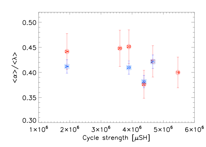
Figure 3: Cycle-averaged tilt angle normalised to cycle-averaged latitude, as a function of cycle strengths, for Kandilli (red circles) and DPD (blue squares) datasets. Note that cycle 24 is covered until 2017.8 in Kandilli, and 2016.0 in DPD.

4 Conclusion

We have found a remarkable similarity between our data covering cycles 1954-2017 and DPD, which provides sunspot group tilt angles for 1973-2016. This demonstrates the great potential of sunspot drawing archives in deriving important spatio-temporal information on sunspot group properties. Despite differences in the tilt angle determination, both datasets compared here have the common feature of careful group identification and the elimination of unipolar and/or very compact, complex groups. Our results do not indicate a clear anti-correlation between $\langle\alpha\rangle/\langle\lambda\rangle$ and the cycle strength, contrary to [(Dasi-Espuig et al. 2010), (Dasi-Espuig et al. 2013), Dasi-Espuig et al. (2010, 2013)]. In a subsequent paper, we will present our work in more detail, also by revisiting Mt. Wilson and Kodaikanal datasets.

References

- [(Baranyi 2015)] Baranyi, T. 2015, MNRAS, 447, 1857
- [(Baranyi et al. 2016)] Baranyi, T., Győri, L., & Ludmány, A. 2016, Solar Phys., 291, 3081
- [Baumann & Solanki (2005)] Baumann, I., & Solanki, S. K. 2005, A&A, 443, 1061
- [(Dasi-Espuig et al. 2010)] Dasi-Espuig, M., Solanki, S. K., Krivova, N. A., Cameron, R., & Peñuela, T. 2010, A&A, 518, A7
- [(Dasi-Espuig et al. 2013)] Dasi-Espuig, M., Solanki, S. K., Krivova, N. A., Cameron, R., & Peñuela, T. 2013, A&A, 556, C3
- [Howard (1991)] Howard, R. F. 1991, Solar Phys., 136, 251
- [(Işık 2015)] Işık, E. 2015, ApJ (Letters), 813, L13
- [(Jiang et al. 2010)] Jiang, J., Işık, E., Cameron, R. H., Schmitt, D., & Schüssler, M. 2010, ApJ, 717, 597
- [Senthamizh Pavai et al. (2015)] Senthamizh Pavai, V., Arlt, R., Dasi-Espuig, M., Krivova, N. A., & Solanki, S.K. 2015, A&A, 584, A73
- [(Tlatov et al. 2013)] Tlatov, A., Illarionov, E., Sokoloff, D., & Pipin, V. 2013, MNRAS, 432, 2975