Space-filling curves of self-similar sets (III): Skeletons

Abstract.

Skeleton is a new notion designed for constructing space-filling curves of self-similar sets. In a previous paper by Dai and the authors [6], it was shown that for all connected self-similar sets with a skeleton satisfying the open set condition, space-filling curves can be constructed. In this paper, we give a criterion of existence of skeletons by using the so-called neighbor graph of a self-similar set. In particular, we show that a connected self-similar set satisfying the finite type condition always possesses skeletons: an algorithm is obtained here.

1. Introduction

Space-filling curves (SFC) have attracted the attention of mathematicians over a century since Peano’s seminal work [18]. In a series of three papers, [20], [6] and the present paper, we give a systematic investigation of space-filling curves for connected self-similar sets.

The notion of skeleton, which can be regarded as a kind of vertex set of a fractal, was first introduced in [7], designed for SFCs of self-affine tiles. The constructions of SFCs in [20] and [6] are based on the assumption that the self-similar set in consideration possesses a skeleton. Precisely, it is shown that

Theorem 1.1 ([6]).

Let $K$ be a connected self-similar set which has a skeleton and satisfies the open set condition, then $K$ admits space-filling curves.

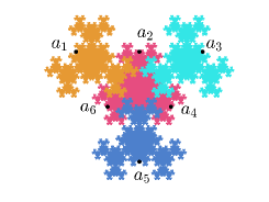
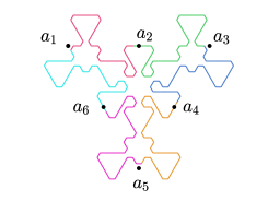
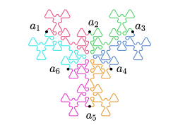
Figure 1. (a) illustrates the four-tile star and $\{a_{1},\dots,a_{6}\}$, a skeleton of it. (b), (c) are the approximating curves constructed by the positive Euler-tour method in [6] with this skeleton. For more details, see [20, Section 7].

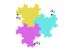
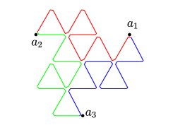
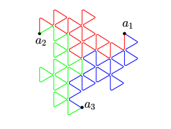
Figure 2. (a) shows the fractal Terdragon and $\{a_{1},a_{2},a_{3}\}$, a skeleton of it. (b), (c) are the approximating curves constructed in [6, Example 5.1] with this skeleton.

The goal of the present paper is to study when a self-similar set has skeletons and how to find them, which is the last part of our theory on constructing SFCs.

Recall that a self-similar set is a non-empty compact set $K$ satisfying the set equation

$$K=\bigcup_{i=1}^{N}S_{i}(K),$$

where $S_{1},\dots,S_{N}$ are contraction similitudes on $\mathbb{R}^{d}$. The family $\{S_{1},\dots,S_{N}\}$ is called an iterated function system, or IFS in short; $K$ is also called the invariant set of the IFS. (See for instance, [11, 9]). For the open set condition, we refer to [9, Section 9.2].

To define the skeleton of a self-similar set, we construct a graph which is a generalization of Hata [10]. Let $\{S_{j}\}_{j=1}^{N}$ be an IFS with invariant set $K$. For any subset $A$ of $K$, we define an undirected graph $H(A)$ as follows:

• The vertex set is $V=\{S_{1},S_{2},\dots,S_{N}\}$;

• There is an edge between $S_{i}$ and $S_{j}$ $(i\neq j)$ if and only if $S_{i}(A)\cap S_{j}(A)\neq\emptyset$.

We call $H(A)$ the Hata graph induced by $A$ (with respect to the IFS $\{S_{1},\dots,S_{N}\}$).

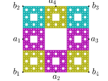
(a) Sierpiński carpet $C$

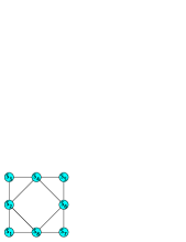
(b) $H(A)$ with $A=C$ or $A=\{b_{1},b_{2},b_{3},b_{4}\}$

(c) $H(A)$ with $A=\{a_{1},a_{2},a_{3},a_{4}\}$

Figure 3. The Hata graphs $H(A)$ of the Sierpiński carpet w.r.t. the IFS $\{S_{i}(x)=\frac{x+d_{i}}{3}\}_{i=1}^{8}$, $\{d_{1},\dots,d_{8}\}=\{0,{\mathbf{i}},2{\mathbf{i}},2{\mathbf{i}}+1,2{\mathbf{i}}+2,{\mathbf{i}}+2,2,1\}$. It is easy to check that both $\{a_{1},\dots,a_{4}\}$ and $\{b_{1},\dots,b_{4}\}$ are skeletons of Sierpiński carpet.

Remark 1.2.

Hata [10] introduced the above graph but fixed $A$ to be $K$. Hata proved that a self-similar set $K$ is connected if and only if the graph $H(K)$ is connected. (An undirected graph $G$ is said to be connected, if for every pair of vertices in $G$ there is a path in $G$ joining them.)

Definition 1.3.

Let $\{S_{j}\}_{j=1}^{N}$ be an IFS such that the invariant set $K$ is connected. We call a finite subset $A$ of $K$ a skeleton of $\{S_{j}\}_{j=1}^{N}$ (or $K$), if the following two conditions are fulfilled:

• $A$ is stable under iteration, that is, $A\subset\bigcup_{j=1}^{N}S_{j}(A)$;

• The Hata graph $H(A)$ is connected.

A skeleton consists of at least two elements if the self-similar set $K$ is not a singleton (Proposition 2.2).

In the previous works, there are two notions closely related to the skeleton, the self-similar zipper and the boundary of a self-similar set, see Remark 1.4 and 1.5.

Remark 1.4.

The word zipper was first used in fractal context by Thurston [24] to denote curves in C which have conformally rigid complement. Later Astala [2] proved that this property is true for any self-similar quasi-interval in $\mathbb{C}$ which is not a line segment. The definition of self-similar zipper with binary signature in Section 2.3 was initially proposed by Aseev and Tetenov [1]. Before that, self-similar zippers of zero signature (without giving them any name) appeared in several papers, including [11, 25, 27]. The graph directed version of zippers, called multizippers, was introduced and studied in [22]. The definition of multizipper is equivalent to the one of linear GIFS proposed by the authors in [20, 6].

Self-similar zippers have skeletons of cardinality $2$ (see Section 2.3). Indeed, many beautiful fractals have self-similar zipper structures, for example, the Heighway dragon and the Gosper island. It is shown [6] that a self-similar zipper, which is called the path-on-lattice IFS in [20], admits space-filling curves provided the open set condition holds. The website [26] provides a nice collection of SFCs of self-similar zippers.

Figure 4. (a) is the Gosper island and a skeleton $\{a_{1},a_{2}\}$. (b), (c) are the approximating curves generated by path-on-lattice IFS, see [20, Example 5.2].

Remark 1.5.

Kigami [15] and Morán [16] have studied the ‘boundary’ of a self-similar set. If the ‘boundary’ is a finite set, it is so-called p.c.f. self-similar set ([14, Definition 1.12]). Clearly a p.c.f. self-similar set always has skeletons. We also note that the notion of skeleton is very close to the ideas used in [5, 21] for building minimal paths in p.c.f. self-similar sets.

Next, we show existence of the skeleton for a more general case. The self-similar sets satisfying finite type condition constitute an important class of fractals (see for instance, [19, 17, 4]). In fact, all the space-filling curves appeared in the literature were constructed for the self-similar sets of finite type. We prove that

Theorem 1.6.

Let $K$ be the invariant set of an IFS satisfying the finite type condition. If $K$ is connected, then $K$ possesses a skeleton.

Proof.

This is an immediate consequence of Theorem 3.3 and Theorem 4.5. ∎

As a consequence of Theorem 1.1 and Theorem 1.6, we conclude that: if a connected self-similar set satisfies both the open set condition and the finite type condition, then it admits space-filling curves, which is the main result of [6].

There do exist self-similar sets without skeletons.

Example 1.1.

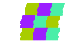
Figure 5. Self-similar set without skeleton

Let $\mathcal{D}=\{d_{1},d_{2},\dots,d_{9}\}=\{0,1,2,{\mathbf{i}},1+{\mathbf{i}},2+{\mathbf{i}},\varepsilon+2{\mathbf{i}},\varepsilon+1+2{\mathbf{i}},\varepsilon+2+2{\mathbf{i}}\}$ where $\varepsilon$ is a small irrational number, for example, $\varepsilon={\sqrt{2}}/{4}$. Kenyon [13] shows that the self-similar set $K$ generated by the IFS $\{S_{i}(z)=(z+d_{i})/3\}_{i=1}^{9}$ is a reptile. In Section 3 we will show that $K$ has no skeleton.

This paper is organized as follows. In Section 2, we give some notation and basic properties of skeletons. In Section 3, we introduce the bifurcation pair and give a criterion for the existence of skeletons. The finite type condition is discussed in Section 4. In the last section we give an algorithm for finding skeletons and we provide some examples.

2. Basic properties of skeletons

In this section, we deduce some basic properties of skeletons. Let ${\mathcal{S}}=\{S_{j}\}_{j=1}^{N}$ be an IFS and $K$ be the invariant set.

2.1. Symbolic space

First, we recall some notations of symbolic space. Denote $\Sigma=\{1,2,\dots,N\}$ and $\mathbb{N}=\{0,1,\dots\}$. For $m\geq 1$, define $\Sigma^{m}=\{1,2\cdots N\}^{m}$ with $\Sigma^{0}=\{\emptyset\}$, and set $\Sigma^{\ast}=\bigcup_{m=0}^{\infty}{\Sigma^{m}}$. Denote $\Sigma^{\mathbb{N}}$ the collection of infinite sequences over $\Sigma$. For ${\boldsymbol{\omega}}=(\omega_{j})_{j=1}^{\infty}\in\Sigma^{\mathbb{N}}$, let ${\boldsymbol{\omega}}|_{n}=\omega_{1}\omega_{2}\dots\omega_{n}$ be the prefix of ${\boldsymbol{\omega}}$ of length $n$. For $i_{1}i_{2}\dots i_{m}\in\Sigma^{*}$, we call

$$[i_{1}i_{2}\dots i_{m}]=\{{\boldsymbol{\omega}}\in\Sigma^{\mathbb{N}}~{};~{}~{}{\boldsymbol{\omega}}|_{m}=i_{1}i_{2}\dots i_{m}\}$$

a cylinder. We denote $S_{i_{1}i_{2}\dots i_{m}}=S_{i_{1}}\circ S_{i_{2}}\circ\cdots\circ S_{i_{m}}$.

Define $\pi:\Sigma^{\mathbb{N}}\rightarrow K$ as

$$\{\pi({\boldsymbol{\omega}})\}=\bigcap_{1}^{\infty}S_{{\boldsymbol{\omega}}|_{m}}(K).$$

Then $\pi$ is a surjection. We call ${\boldsymbol{\omega}}$ a coding of $x$ if $\pi({\boldsymbol{\omega}})=x$.

The shift map $\sigma:\Sigma^{\mathbb{N}}\rightarrow\Sigma^{\mathbb{N}}$ is defined as $\sigma((\omega_{k})_{k\geq 1})=(\omega_{k})_{k\geq 2}$.

For $k\in\Sigma$, we define $\sigma_{k}:\Sigma^{\mathbb{N}}\rightarrow\Sigma^{\mathbb{N}}$ as

$$\sigma_{k}(\omega_{1}\omega_{2}\omega_{3}\dots)=k\omega_{1}\omega_{2}\omega_{3}\dots.$$

It holds that  $\pi\circ\sigma_{k}=S_{k}\circ\pi$ (see [11] or [15].)

2.2. Skeleton of an iteration of an IFS

Denote the Hata graph of $K$ by $H=H(K)$. We shall denote by $\{S_{i},S_{j}\}$ the edge in $H$ connecting $S_{i}$ and $S_{j}$. In an undirected graph $G$, we will use a sequence of distinct vertices in $G$ to indicate a path, if any two consecutive vertices in the sequence are joined by an edge.

We define the $n$-th iteration of $\mathcal{S}$ to be the IFS

$${\mathcal{S}}^{n}=\{S_{I};~{}I\in\Sigma^{n}\}.$$

It is well-known that ${\mathcal{S}}^{n}$ shares the same invariant sets as ${\mathcal{S}}$ (see Falconer [9]). Similarly, we have

Proposition 2.1.

If $A$ is a skeleton of $\mathcal{S}$, then $A$ is also a skeleton of $\mathcal{S}^{n}$.

Proof.

Note that $H({\mathcal{S}}^{n},A)$ is the Hata graph of $A$ related to ${\mathcal{S}}^{n}$. We prove that $A\subset\bigcup_{I\in\Sigma^{k}}S_{I}(A)$ and $H({\mathcal{S}}^{k},A)$ is connected for all $k\geq 1$ by induction.

Clearly the statement holds for $k=1$ by the definition of skeleton. Suppose the statement hold for $k=n-1$, that is, $A\subset\bigcup_{I^{\prime}\in\Sigma^{n-1}}S_{I^{\prime}}(A)$ and $H({\mathcal{S}}^{n-1},A)$ is connected. We shall show the statement holds for $k=n$.

First, we observe that

$$A\subset\bigcup_{i=1}^{N}S_{i}(A)\subset\bigcup_{i=1}^{N}S_{i}\left(\bigcup_{I^{\prime}\in\Sigma^{n-1}}S_{I^{\prime}}(A)\right)=\bigcup_{I\in\Sigma^{n}}S_{I}(A).$$

Next, we show that $H(\mathcal{S}^{n},A)$ is connected. To this end, we need only show that for any two words $I=i_{1}\dots i_{n},~{}J=j_{1}\dots,j_{n}\in\Sigma^{n}$, there is a path in $H({\mathcal{S}}^{n},A)$ connecting $S_{I}$ and $S_{J}$. Denote $I^{\prime}=i_{2}\dots i_{n}$, $J^{\prime}=j_{2}\dots j_{n}$.

Claim 1. The restriction of $H({\mathcal{S}}^{n},A)$ on $\{i\}\times\Sigma^{n-1}$ is connected.

By induction hypothesis, there exist $L_{1},\dots,L_{k}\in\Sigma^{n-1}$ such that $S_{I^{\prime}},S_{L_{1}},\dots,S_{L_{k}},S_{J^{\prime}}$ is a path in $H({\mathcal{S}}^{n-1},A)$, so

$$S_{i_{1}I^{\prime}},S_{i_{1}L_{1}},\dots,S_{i_{1}L_{k}},S_{i_{1}J^{\prime}}$$

is a path joining $S_{I}$ and $S_{i_{1}J^{\prime}}$ in $H({\mathcal{S}}^{n},A)$.

Claim 2. $S_{I}$ and $S_{J}$ are connected in $H({\mathcal{S}}^{n},A)$ if $\{S_{i_{1}},S_{j_{1}}\}$ is an edge in $H({\mathcal{S}},A)$.

The assumption implies that $S_{i_{1}}(A)\cap S_{j_{1}}(A)\neq\emptyset$, so

$$\left(\bigcup_{I^{\prime\prime}\in\Sigma^{n-1}}S_{i_{1}I^{\prime\prime}}(A)\right)\cap\left(\bigcup_{J^{\prime\prime}\in\Sigma^{n-1}}S_{j_{1}J^{\prime\prime}}(A)\right)\neq\emptyset,$$

so $S_{i_{1}I^{\prime\prime}}(A)\cap S_{j_{1}J^{\prime\prime}}(A)\neq\emptyset$ for some $I^{\prime\prime},J^{\prime\prime}$ with length $n-1$; namely, there is an edge connecting $S_{i_{1}I^{\prime\prime}}$ and $S_{j_{1}J^{\prime\prime}}$. Therefore, the path from $S_{I}$ to $S_{i_{1}I^{\prime\prime}}$ (by Claim 1), the edge $\{S_{{i_{1}}I^{\prime\prime}},S_{{j_{1}}J^{\prime\prime}}\}$, and the path from $S_{j_{1}J^{\prime\prime}}$ to $S_{J}$ (again by Claim 1) form a path from $S_{I}$ to $S_{J}$.

Now we deal with the general case. Since $H({\mathcal{S}},A)$ is connected, there exists a path connected the vertices $S_{i_{1}}$ and $S_{j_{1}}$. Using Claim 2 repeatedly, we obtain that $H({\mathcal{S}}^{n},A)$ is connected. ∎

Proposition 2.2.

If a self-similar set $K$ has a skeleton $A=\{a\}$, then $K=\{a\}$.

Proof.

Since the Hata graph $H(A)$ is connected, $S_{i}(a)=S_{j}(a)$ if there is an edge between the vertices $S_{i}$ and $S_{j}$ in $H(A)$, so $S_{1}(a)=\cdots=S_{N}(a)$. This together with $A\subset\bigcup_{j=1}^{N}S_{j}(A)$ implies that $a$ is the fixed point of $S_{j}$ for every $j=1,\dots,N$. It follows that $K=\{a\}$. ∎

2.3. Self-similar zippers

Let $(S_{j})_{j=1}^{N}$ be an IFS where the mappings are ordered. If there exists a set $\{x_{0},\dots,x_{N}\}$ of points and a sequence $(\beta_{1},\dots,\beta_{N})\in\{-1,1\}^{N}$ such that the mapping $S_{j}$ takes the pair $(x_{0},x_{N})$ into the pair $(x_{j-1},x_{j})$ if $s_{j}=1$, and into the pair $(x_{j},x_{j-1})$ if $s_{j}=-1$, then we call $\{S_{j}\}_{j\in\Sigma}$ a self-similar zipper. $\{x_{0},\dots,x_{N}\}$ is called the set of vertices and call $(\beta_{1},\dots,\beta_{N})$ the vector of signature. It is easy to prove that $A=\{x_{0},x_{N}\}$ is a skeleton of the IFS.

The definition of self-similar zipper above is introduced by [1]. It is worth to mention that [23] considers a self-similar dendrite which cannot be the attractor of any zipper. At the same time, it has a skeleton, therefore it admits a space-filling curve, as it follows from Theorem 1.1.

3. Bifurcation pairs

In this section, we give a necessary and sufficient condition of the existence of a skeleton. Recall that $\Sigma=\{1,2,\dots,N\}$. Let $K$ be the connected self-similar set generated by an IFS $\{S_{i}\}_{i\in\Sigma}$.

Denote the Hata graph of $K$ by $H=H(K)$. A sequence $(\omega_{j})_{j=1}^{\infty}$ is called eventually periodic, if there exists $p\geq 1$ such that $(\omega_{j})_{j=p}^{\infty}$ is periodic.

Definition 3.1.

For $e=\{S_{i},S_{j}\}\in H$, a pair ${\boldsymbol{\omega}}=(\omega_{k})_{k\geq 1},{\boldsymbol{\gamma}}=(\gamma_{k})_{k\geq 1}\in\Sigma^{\mathbb{N}}$ is called a bifurcation pair of $e$, if both sequences are eventually periodic, and $\omega_{1}=i,\gamma_{1}=j$, $\pi({\boldsymbol{\omega}})=\pi({\boldsymbol{\gamma}})$.

Let $R$ be a subgraph of the Hata graph $H$. We call $R$ a spanning graph of $H$ if $R$ is connected, and $R$ has the same vertex set as $H$.

Lemma 3.2.

Let $B$ be a finite subset of $K$ such that $B\subset\bigcup_{j=1}^{N}S_{j}(B)$. Then for any point $x\in B$, $x$ has an eventually periodic coding.

Proof.

Since $B$ is stable under iteration, for any $x\in B$, there exist $i_{1}\in\Sigma$ and $x_{1}\in B$ such that $x=S_{i_{1}}(x_{1})$. Inductively, let $i_{k+1}\in\Sigma$ and $x_{k+1}\in B$ such that $x_{k}=S_{i_{k+1}}(x_{k+1})$. Since $B$ is finite, there must exist $m,\ell\geq 1$ such that $x_{\ell}=x_{\ell+m}$. Hence $i_{1}\dots i_{\ell}(i_{\ell+1}\dots i_{\ell+m})^{\infty}$ is an eventually periodic coding of $x$. ∎

Theorem 3.3.

Let $K$ be a connected self-similar set. Then $K$ possesses a skeleton if and only if there exists a spanning graph $R\subset H(K)$ such that every edge $e\in R$ admits a bifurcation pair.

Proof.

First, we prove the ‘if’ part. Let $R$ be a spanning graph of $H(K)$ such that each edge $e\in R$ admits a bifurcation pair. Pick $e=\{S_{i},S_{j}\}\in R$ and let $\{{\boldsymbol{\omega}}_{e},{\boldsymbol{\gamma}}_{e}\}$ be a bifurcation pair of $e$. Then

$$\mathcal{B}_{e}=\{\sigma^{k}({\boldsymbol{\omega}}_{e});~{}k\in\mathbb{N}\}\cup\{\sigma^{k}({\boldsymbol{\gamma}}_{e});~{}k\in\mathbb{N}\},$$

the union of orbits of ${\boldsymbol{\omega}}$ and ${\boldsymbol{\gamma}}$ under $\sigma$, is a finite set. We claim that

(3.1) $$A=\bigcup_{e\in R}{\pi(\mathcal{B}_{e})}$$

is a skeleton of $K$.

First, we show that the Hata graph $H(A)$ contains $R$ as a subgraph, and hence $H(A)$ is connected since $R$ is spanning and connected. For $e=\{S_{i},S_{j}\}\in R$, denote $x_{e}=\pi({\boldsymbol{\omega}})=\pi({\boldsymbol{\gamma}})$. Then

$$x_{e}=S_{i}\circ\pi(\sigma({\boldsymbol{\omega}}))=S_{j}\circ\pi(\sigma({\boldsymbol{\gamma}}))\in S_{i}(A)\cap S_{j}(A),$$

which implies that $e\in H(A)$. Therefore, $R$ is a subgraph of $H(A)$.

Secondly, we show that $A$ is stable. Take $x\in A$, $x$ can be written as $x=\pi(\sigma^{k}({\boldsymbol{\omega}}_{e}))$ for some $e\in R$. Let $\ell$ be the $(k+1)$-th entry of the sequence ${\boldsymbol{\omega}}_{e}$, then

$$x=\pi(\ell\sigma^{k+1}({\boldsymbol{\omega}}_{e}))=S_{\ell}\circ\pi(\sigma^{k+1}({\boldsymbol{\omega}}_{e}))\in S_{\ell}(A),$$

which verifies that $A\subset\cup_{j=1}^{N}S_{j}(A)$.

Now we prove the ‘only if’ part. Suppose $A$ is a skeleton of $K$. Then $R=H(A)$ is a spanning graph of $H(K)$. We claim that every edge of $R$ admits a bifurcation pair and hence $R$ is the desired spanning graph of $H(K)$.

Let $e=\{S_{i},S_{j}\}$ be an edge of $R$. Let $z\in S_{i}(A)\cap S_{j}(A)$. Then there exist $x,y\in A$ such that $z=S_{i}(x)=S_{j}(y)$. By Lemma 3.2, there exist eventually periodic sequences ${\boldsymbol{\omega}},{\boldsymbol{\gamma}}\in\Sigma^{\mathbb{N}}$ such that $x=\pi({\boldsymbol{\omega}}),y=\pi({\boldsymbol{\gamma}})$. It follows that $i\boldsymbol{\omega}$ and $j{\boldsymbol{\gamma}}$ are two eventually periodic codings of $z$, in other words, $\{i{\boldsymbol{\omega}},j{\boldsymbol{\gamma}}\}$ is a bifurcation pair. The theorem is proved. ∎

To close this section, we show that the reptile $K$ in Example 1.1 does not have a skeleton.

Suppose on the contrary that $K$ has a skeleton $A$. To guarantee that the Hata graph $H(A)$ is connected, there must exist $i^{*}\in\{1,2,3\}$, $j^{*}\in\{4,5,6\}$ such that $S_{i^{*}}(A)\cap S_{j^{*}}(A)\neq\emptyset$. Take a point $\left(\begin{matrix}x\\ y\end{matrix}\right)$ from the intersection. It is seen that we must have $y=1/3$.

By Theorem 3.3, the point $\left(\begin{matrix}x\\ 1/3\end{matrix}\right)$ has two eventually codings with initial letter $i^{*}$ and $j^{*}$ respectively. It follows that

$$\left(\begin{array}[]{c}x\\ 1/3\end{array}\right)=\sum_{k=1}^{\infty}3^{-k}\left(\begin{array}[]{c}x_{k}\\ y_{k}\end{array}\right)=\sum_{k=1}^{\infty}3^{-k}\left(\begin{array}[]{c}\tilde{x}_{k}\\ \tilde{y}_{k}\end{array}\right),$$

where $\left(\begin{matrix}x_{1}\\ y_{1}\end{matrix}\right)=d_{i^{*}}$, $\left(\begin{matrix}\tilde{x}_{1}\\ \tilde{y}_{1}\end{matrix}\right)=d_{j^{*}}$, and $\left(\begin{matrix}x_{k}\\ y_{k}\end{matrix}\right),\left(\begin{matrix}\tilde{x}_{k}\\ \tilde{y}_{k}\end{matrix}\right)\in\mathcal{D}$ for $k\geq 2$. Focusing on the second coordinate, we see that $y_{1}=0$, $\tilde{y}_{1}=1$ and $y_{k},\tilde{y}_{k}\in\{0,1,2\}$ for $k\geq 2$. From $1/3=\sum_{k\geq 1}3^{-k}y_{k}=\sum_{k\geq 1}3^{-k}\tilde{y}_{k}$ we deduce that

$$y_{k}=2,\ \tilde{y}_{k}=0,\text{ for }k\geq 2.$$

Then

$$\left(\begin{matrix}x_{k}\\ y_{k}\end{matrix}\right)\in\{d_{7},d_{8},d_{9}\}\text{ and }\left(\begin{matrix}\tilde{x}_{k}\\ \tilde{y}_{k}\end{matrix}\right)\in\{d_{1},d_{2},d_{3}\},\quad k\geq 2,$$

and so that $x_{k}\in\{\varepsilon,\varepsilon+1,\varepsilon+2\}$ and $\tilde{x}_{k}\in\{0,1,2\}$ for $k\geq 2$. Since $(x_{k})_{k\geq 1}$ and $(\tilde{x}_{k})_{k\geq 1}$ are eventually periodic, we have that $\sum 3^{-k}x_{k}$ is irrational and $\sum 3^{-k}\tilde{x}_{k}$ is rational, which contradicts that $\sum 3^{-k}x_{k}=\sum 3^{-k}\tilde{x}_{k}$. This contradiction completes the proof.

4. Finite type condition

In this section, we deal with self-similar sets of finite type, and then Theorem 1.6 can be proved.

4.1. Terminology of Graphs

First, we recall some terminologies of graph theory, see for instance, [3]. Let $H$ be a directed graph. We shall use $\{e_{1},\dots,e_{k}\}$ to denote a walk consisting of the edges $e_{1},\dots,e_{k}$. (For the definition of walk see [3, Definition 1.5.1].) We call the starting vertex and terminate vertex of a walk the origin and terminus, respectively. The walk is closed if the origin of $e_{1}$ and the terminus of $e_{k}$ coincide. A walk is called a trail, if all the edges appearing in the walk are distinct. A trail is called a path if all the vertices are distinct. A closed path is called a cycle.

4.2. Neighbor maps

Recall that $\Sigma=\{1,\dots,N\}$ and $\Sigma^{\ast}=\bigcup_{m=0}^{\infty}{\Sigma^{m}}$. For $I,J\in\Sigma^{*}$, we say that $I$ and $J$ are non-comparable, if neither $I$ is a prefix of $J$, nor $J$ is a prefix of $I$. We use $|I|$ to denote the length of the word $I$, and use $I^{-}$ to denote the word obtained by deleting the last letter of $I$.

Let $\{S_{i}\}_{i\in\Sigma}$ be an IFS with invariant set $K$. Without loss of generality, we assume that $0\in K$. Denote the contraction ratio of $S_{j}$ by $r_{j}$, and denote $r_{I}$ the contraction ratio of the map $S_{I}$. Set

$$r_{*}=\min_{j\in\Sigma}|r_{j}|,\quad r^{*}=\max_{j\in\Sigma}|r_{j}|.$$

Definition 4.1.

For a non-comparable pair $I,J\in\Sigma^{*}$, the map

$$f(z)=S_{J}^{-1}\circ S_{I}(z)$$

is called a neighbor map, and we call it a feasible neighbor map if

$$r_{*}<(r_{J})^{-1}r_{I}\leq(r_{*})^{-1}.$$

A feasible neighbor map describes the relative position of two cylinders which have about the same size. Let ${\mathcal{N}}_{0}$ be the collection of feasible neighbor maps. For any $i,j\in\Sigma$ with $i\neq j$, we call $S_{j}^{-1}\circ S_{i}$ the basic neighbor maps. Clearly all basic neighbor maps are feasible.

4.3. Neighbor graph

The neighbor graph is a directed graph with vertex set ${\mathcal{N}}_{0}$. Let $\epsilon$ be the empty word, and we set $S_{\epsilon}=id$ to be the identity map for convention. For $f,g\in{\mathcal{N}}_{0}$, we say that there is an edge from $f$ to $g$, if there exist $i\in\Sigma$ such that

$$f\circ S_{i}=g\text{ or }S_{i}^{-1}\circ f=g;$$

in the first case, we denote the edge by $(\epsilon,i)$, or $(f,\epsilon,i,g)$, while in the second case, we name the edge by $(i,\epsilon)$, or $(f,i,\epsilon,g)$. We call the graph defined above the complete neighbor graph, and denote it by $\Delta_{0}$.

Definition 4.2.

An IFS $\{S_{j}\}_{j\in\Sigma}$ is said to satisfy the finite type condition if

$${\mathcal{N}}=\left\{f\in{\mathcal{N}}_{0};~{}f(K)\cap K\neq\emptyset\right\}$$

is a finite set. We call the restriction of $\Delta_{0}$ on ${\mathcal{N}}$, denoted by $\Delta$, the neighbor graph.

The following lemma is folklore. We give a proof for the sake of readers.

Lemma 4.3.

(i) For any $f\in{\mathcal{N}}_{0}$, there is a walk in $\Delta_{0}$ starting at some basic neighbor map and terminating at $f$. (If $f$ is a basic neighbor map, then it is an empty walk starting from itself. )

(ii) For any $f\in{\mathcal{N}}$, there is at least one edge in $\Delta$ emanating from $f$.

Proof.

(i) Suppose $f=S_{J}^{-1}\circ S_{I}\in{\mathcal{N}}_{0}$ is a feasible neighbor map, we prove the lemma by induction on $|I|+|J|$. The lemma is clearly true if $|I|+|J|=2$, since $f$ itself is a basic neighbor map. Let $r$ be the contraction ratio of $f$.

If $|r|>1$, then $h=S_{J^{-}}^{-1}\circ S_{I}$ is clearly a feasible neighbor map, and there is an edge $(h,j^{*},\epsilon,f)$ from $h$ to $f$ where $j^{*}$ is the last letter of $J$. By induction, there is a walk starting at some basic neighbor map and terminating at $h$, and this walk can be extended to $f$.

If $|r|\leq 1$, let $h=S_{J}^{-1}\circ S_{I^{-}}$, and the above discussion still holds.

(ii) Without loss of generality, let us assume that the contraction ratio of $f$ is no less than $1$. Pick $x\in f(K)\cap K$, then there exists $j\in\Sigma$ such that $x\in f\circ S_{j}(K)$. Clearly $f\circ S_{j}\in{\mathcal{N}}$ and there is an edge $(\epsilon,S_{j})$ from $f$ to $f\circ S_{j}$. ∎

4.4. Searching bifurcation pairs with the neighbor graph

The existence of bifurcation pair can be characterized in terms of the neighbor graph.

Lemma 4.4.

An edge $e=\{S_{i},S_{j}\}$ of the Hata graph $H(K)$ admits a bifurcation pair if there is an eventually periodic walk on $\Delta$ emanating from the basic neighbor map $S_{i}^{-1}\circ S_{j}$ or $S_{j}^{-1}\circ S_{i}$.

Proof.

Let $(\omega_{n})_{n\geq 1}$ be an eventually periodic walk emanating from $S_{i}^{-1}\circ S_{j}$. This means that there exist $I_{0},I_{1},J_{0},J_{1}\in\Sigma^{*}$ such that $S_{iI_{0}I_{1}^{k}}^{-1}S_{jJ_{0}J_{1}^{k}}\in{\mathcal{N}}$ for all $k\geq 1$, so

(4.1) $$S_{iI_{0}I_{1}^{k}}(K)\cap S_{jJ_{0}J_{1}^{k}}(K)\neq\emptyset$$

for all $k\geq 1$. Let $x$ be the point with the coding $iI_{0}(I_{1})^{\infty}$, then by (4.1), $x$ has a second coding $jJ_{0}(J_{1})^{\infty}$. Therefore, $\{iI_{0}(I_{1})^{\infty},jJ_{0}(J_{1})^{\infty}\}$ is a bifurcation pair of $e=\{S_{i},S_{j}\}$. ∎

As an immediate consequence of the above lemma, we have

Theorem 4.5.

Let $K$ be a self-similar set satisfying the finite type condition. Let $H=H(K)$ be the Hata graph. Then every edge $e\in H$ admits a bifurcation pair.

Proof.

Suppose $e=(S_{i},S_{j})\in H(K)$, then $S_{j}(K)\cap S_{i}(K)\neq\emptyset$. Thus $f=S_{j}^{-1}\circ S_{i}\in{\mathcal{N}}$.

By Lemma 4.3 (ii), there is an infinite walk in $\Delta$ starting from $f$; moreover, this walk must be eventually periodic since $\Delta$ is a finite graph. Finally, by Lemma 4.4, $e$ admits a bifurcation pair. ∎

Another consequence of Lemma 4.4 is the following.

Corollary 4.6.

Let $K$ be a connected self-similar set. If there exists a spanning graph $R\subset H(K)$ such that, for every edge $e=\{S_{i},S_{j}\}\in R$, there is an eventually periodic walk on $\Delta$ emanating from the neighbor map $S_{i}^{-1}\circ S_{j}$ or $S_{j}^{-1}\circ S_{i}$, then $K$ possesses a skeleton.

5. Algorithm and Examples

In this section, we formulate an algorithm to obtain skeletons for a self-similar set of finite type. Besides, we will give three examples related to the so-called single-matrix IFS.

5.1. Algorithm

Let $\mathcal{S}=\{S_{j}\}_{j\in{\Sigma}}$ be an IFS such that the invariant set $K$ is connected and $\mathcal{S}$ satisfies the finite type condition. Summarizing the results in the previous sections, we give an algorithm consisting of the following four steps:

$(i)$ Compute the neighbor graph $\Delta$;

$(ii)$ Compute the Hata graph $H(K)$, and choose a spanning graph $R$;

$(iii)$ For each $e\in R$, find a bifurcation pair of $e$ by Theorem 4.5;

$(iv)$ Construct a skeleton according to (3.1).

5.2. Neighbor graph of IFS with uniform contraction ratio

If all the contraction ratios $r_{j}$ of the similitudes in an IFS have the same value, then the neighbor graph can be simplified as follows (see [4]). First, the sets ${\mathcal{N}}_{0}$ and ${\mathcal{N}}$ can be reduced to

$$\mathcal{N}_{0}=\bigcup_{n=1}^{\infty}\left\{S_{J}^{-1}S_{I};~{}~{}{I},{J}\in\Sigma^{n},i_{1}\neq j_{1}\right\},$$

$${\mathcal{N}}=\{f\in{\mathcal{N}}_{0};~{}f(K)\cap K\neq\emptyset\}.$$

Secondly, the neighbor graph can be simplified as follows: For $f,g\in{\mathcal{N}}_{0}$, there is an edge from $f$ to $g$, if there exists a pair $i,j\in\Sigma$ such that

$$S_{j}^{-1}\circ f\circ S_{i}=g;$$

in this case, we name the edge by $(f,j,i,g)$, or label the edge by $(j,i)$ in short.

5.3. Single-matrix IFS

A single-matrix IFS is a special type of IFS with uniform ratio giving by

(5.1) $$S_{i}(z)=rM(z+d_{i}),\quad i=1,\dots,N,$$

where $0<r<1$ and $M$ is an orthogonal matrix, see [12]. Let us denote ${\mathcal{D}}=\{d_{1},\dots,d_{N}\}$, and define

$${\mathcal{D}}^{*}=\bigcup_{n=1}^{\infty}\left\{\sum_{k=0}^{n-1}(rM)^{-k}x_{k};~{}x_{k}\in D-D\right\}.$$

By induction, one can show that

$${\mathcal{N}}_{0}=\{z\mapsto z+b;~{}b\in{\mathcal{D}}^{*}\}.$$

In particular, if ${\mathcal{D}}^{*}$ is uniformly discrete, that is, $\inf_{x,y\in{\mathcal{D}}^{*}}|x-y|>0$, then

the set $\{|b|<T;~{}b\in{\mathcal{D}}^{*}\}$ is a finite set for any $T>0$,
and hence the IFS satisfies the finite type condition.

5.4. Examples

Example 5.1.

Skeleton of Terdragon. Recall the IFS of Terdragon is

$$S_{1}(z)=\lambda z+1,~{}S_{2}(z)=\lambda z+\omega,S_{3}(z)=\lambda z+\omega^{2},$$

where $\lambda=\exp(\pi{\mathbf{i}}/6)/\sqrt{3}$ and $\omega=\exp(2\pi{\mathbf{i}}/3)$. The IFS is of the form (5.1) with $rM=\exp({\mathbf{i}}\pi/6)/\sqrt{3}$, and

$${\mathcal{D}}=\sqrt{3}\exp(-{\mathbf{i}}\pi/6)\cdot\{1,\omega,\omega^{2}\}.$$

Since $(rM)^{-1}=1-\omega$, it is easy to show that ${\mathcal{D}}^{*}$ is a subset of the lattice $\mathbb{Z}+\mathbb{Z}\omega$ and hence it is uniformly discrete.

$(i)$ The feasible neighbor map set is

$${\mathcal{N}}=\{f_{1},f_{2},f_{3},f_{4},f_{5},f_{6}\}:=\{S_{2}^{-1}\circ S_{3},S_{1}^{-1}\circ S_{3},S_{1}^{-1}\circ S_{2},S_{2}^{-1}\circ S_{1},S_{3}^{-1}\circ S_{1},S_{3}^{-1}\circ S_{2}\}.$$

The neighbor graph $\Delta$ (see Figure 6) is

$$f_{1}\stackrel{{\scriptstyle(3,1)}}{{\longrightarrow}}f_{1},\ f_{1}\stackrel{{\scriptstyle(3,2)}}{{\longrightarrow}}f_{2},\ f_{2}\stackrel{{\scriptstyle(2,1)}}{{\longrightarrow}}f_{2},\ f_{2}\stackrel{{\scriptstyle(3,1)}}{{\longrightarrow}}f_{3};$$

$$f_{3}\stackrel{{\scriptstyle(2,3)}}{{\longrightarrow}}f_{3},\ f_{3}\stackrel{{\scriptstyle(2,1)}}{{\longrightarrow}}f_{6},\ f_{6}\stackrel{{\scriptstyle(1,3)}}{{\longrightarrow}}f_{6},\ f_{6}\stackrel{{\scriptstyle(2,3)}}{{\longrightarrow}}f_{5};$$

$$f_{5}\stackrel{{\scriptstyle(1,2)}}{{\longrightarrow}}f_{5},\ f_{5}\stackrel{{\scriptstyle(1,3)}}{{\longrightarrow}}f_{4},\ f_{4}\stackrel{{\scriptstyle(3,2)}}{{\longrightarrow}}f_{4},\ f_{4}\stackrel{{\scriptstyle(1,2)}}{{\longrightarrow}}f_{1}.$$

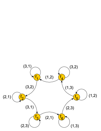
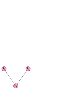
Figure 6. (a): Neighbor graph of Terdragon. (b): Hata graph $H$ of Terdragon.

$(ii)$ We choose $R=H$.

(1) The first skeleton (see Figure 2 (a)). For the three edges $\{S_{1},S_{2}\}$, $\{S_{2},S_{3}\}$ and $\{S_{3},S_{1}\}$ of $R$, we choose the self-loops of $f_{3}=S_{1}^{-1}\circ S_{2},f_{1}=S_{2}^{-1}\circ S_{3},f_{5}=S_{3}^{-1}\circ S_{1}$ respectively, then we obtain the associated bifurcation pairs $\{12^{\infty},\ 23^{\infty}\},\ \{23^{\infty},\ 31^{\infty}\},\ \{31^{\infty},12^{\infty}\}$ respectively. Notice that $\pi(12^{\infty})=\pi(23^{\infty})=\pi(31^{\infty})$=0. So, we obtain the following skeleton

$$\{a_{1},a_{2},a_{3}\}=\pi\{1^{\infty},2^{\infty},3^{\infty}\}=\{S_{3}^{-1}(0),S_{1}^{-1}(0),S_{2}^{-1}(0)\}=\{-\omega^{2},-1,-\omega\}/\lambda.$$

This skeleton is used in [8] and [6].

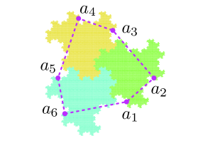
Figure 7. Another skeleton of Terdragon

(2) The second skeleton (see Figure 7). Notice that

$$\big{(}(3,2)(3,1)(2,1)(2,3)(1,3)(1,2)\big{)}^{\infty}$$

is a infinite repetition of a cycle in $\Delta$ passing all the vertices. For $\{S_{2},~{}S_{3}\}\in R$, we regard $f_{1}=S_{2}^{-1}\circ S_{3}$ as the starting point of the above cycle. Then the bifurcation pair associated to $\{S_{2},~{}S_{3}\}$ is $\{2(332211)^{\infty},3(211332)^{\infty}\}$. Similarly, the other two bifurcation pairs associated to $\{S_{1},~{}S_{2}\}$ and $\{S_{3},~{}S_{1}\}$ are $\{1(221133)^{\infty},2(133221)^{\infty}\}$ and $\{3(113322)^{\infty},1(322113)^{\infty}\}$, respectively. Denote ${\boldsymbol{\omega}}=(332211)^{\infty}$, then the resulting skeleton is (see Figure 7)

$$\begin{array}[]{rl}&\{a_{1},a_{2},a_{3},a_{4},a_{5},a_{6}\}=\pi\{\sigma^{k}({\boldsymbol{\omega}});k=0,\dots,5\}\\ =&\{\frac{6}{7}-\frac{4\sqrt{3}}{7}{\mathbf{i}},\frac{12}{7}-\frac{\sqrt{3}}{7}{\mathbf{i}},\frac{3}{7}+\frac{5\sqrt{3}}{7}{\mathbf{i}},-\frac{9}{14}+\frac{13\sqrt{3}}{14}{\mathbf{i}},-\frac{9}{7}-\frac{\sqrt{3}}{7}{\mathbf{i}},-\frac{15}{14}-\frac{11\sqrt{3}}{14}{\mathbf{i}}\}.\end{array}$$

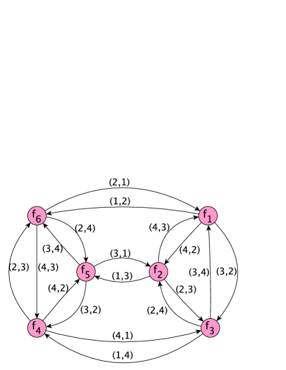
Figure 8. Neighbor graph of Four tile star restricted on basic neighbor maps.

Example 5.2.

Skeleton of the four-tile star. The associated IFS is

$$S_{1}(x)=-\frac{1}{2}x,\ S_{2}(x)=-\frac{1}{2}x-{\mathbf{i}},\ S_{3}(x)=-\frac{1}{2}x+\exp(\frac{5\pi{\mathbf{i}}}{6}),\ S_{4}(x)=-\frac{1}{2}x+\exp(\frac{\pi{\mathbf{i}}}{6}).$$

By the same argument of the previous example, the four-tile star also satisfies the finite type condition.

$(i)$ Figure 8 illustrates a subgraph of the neighbor graph restricted on the six basic neighbor maps $f_{1},\dots,f_{6}$ given by

$$f_{1}=f_{6}^{-1}=S_{1}^{-1}\circ S_{2},\ f_{2}=f_{5}^{-1}=S_{1}^{-1}\circ S_{3},\ f_{3}=f_{4}^{-1}=S_{1}^{-1}\circ S_{4}.$$

$(ii)$ The Hata graph $H$ is depicted in Figure 9 (b), and the spanning graph we choose is

$$R=\{\{S_{1},S_{2}\},\{S_{1},S_{3}\},\{S_{1},S_{4}\}\}.$$

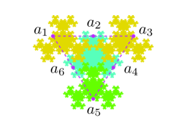
(a) Four-tile star

(b) Hata graph $H$

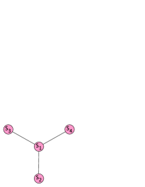
(c) A spanning graph $R$

Figure 9. Four-tile star.

$(iii)$ To find a bifurcation pair of $\{S_{1},S_{2}\}$, we need an eventually walk starting from $f_{1}=S_{1}^{-1}\circ S_{2}$. We choose $\big{(}(1,2),(2,1)\big{)}^{\infty}$ which is the infinite repetition of a cycle. Then we have the bifurcation pairs $\{1(12)^{\infty},2(21)^{\infty}\}$. Similarly, we get the bifurcation pairs of the other two edges $\{S_{1},S_{3}\}$ and $\{S_{1},S_{4}\}$, which are $\{1(13)^{\infty},3(31)^{\infty}\},\ \{1(14)^{\infty},4(41)^{\infty}\},$ respectively.

$(iv)$ The resulted skeleton is

$$\begin{array}[]{rl}\{a_{1},a_{2},a_{3},a_{4},a_{5},a_{6}\}&=\pi\{(31)^{\infty},(12)^{\infty},(41)^{\infty},(13)^{\infty},(21)^{\infty},(14)^{\infty}\}\\ &=\{\frac{-2\sqrt{3}+2{\mathbf{i}}}{3},\frac{2{\mathbf{i}}}{3},\frac{2\sqrt{3}+2{\mathbf{i}}}{3},\frac{\sqrt{3}-{\mathbf{i}}}{3},\frac{-4{\mathbf{i}}}{3},\frac{-\sqrt{3}-{\mathbf{i}}}{3}\}.\end{array}$$

(See Figure 9 (a).)

Example 5.3.

Space-filling curves of Sierpiński carpet. Here we display the SFCs constructed from different skeletons of Sierpiński carpet by using the postive Euler-tour method in [6, Section 5].

• We choose the four vertices $\{b_{1},b_{2},b_{3},b_{4}\}$ as a skeleton (Figure 3 (a)), then we get the space-filling curve as Figure 10.

  

  

  

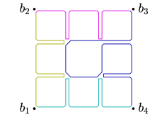
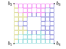
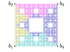
  Figure 10. The first three approximations of SFC of Sierpiński carpet with four vertice as a skeleton.

• We choose three vertice $\{b_{1},b_{2},b_{4}\}$ as a skeleton (Figure 3 (a)). Figure 11 gives the first three approximations of the SFC.

  

  

  

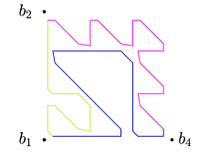
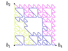
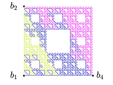
  Figure 11. The first three approximations of SFC of Sierpiński carpet with three vertices as a skeleton.

• Consider the skeleton of four middle points $\{a_{1},a_{2},a_{3},a_{4}\}$ (Figure 3 (a)). The according approximation curves are shown in Figure 12. A detailed discussion of this SFC can be found in [6, Example 5.2].

  

  

  

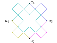
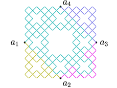
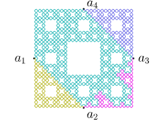
  Figure 12. The first three approximations of SFC of Sierpiński carpet with middle points as a skeleton.

Acknowledgement

We thank the anonymous referees for valuable suggestions and comments, especially that concerns the self-similar zipper.

References

- [1] V. V. Aseev, A. V. Tetenov, and A. S. Kravchenko, Self-similar Jordan curves on the plane, Sibirsk. Mat. Zh., 44 (2003), pp. 481–492.
- [2] K. Astala, Self-similar zippers, in Holomorphic functions and moduli, Vol. I (Berkeley, CA, 1986), vol. 10 of Math. Sci. Res. Inst. Publ., Springer, New York, 1988, pp. 61–73.
- [3] R. Balakrishnan and K. Ranganathan, A textbook of graph theory, Universitext, Springer-Verlag, New York, 2000.
- [4] C. Bandt and M. Mesing, Self-affine fractals of finite type, in Convex and fractal geometry, vol. 84 of Banach Center Publ., Polish Acad. Sci. Inst. Math., Warsaw, 2009, pp. 131–148.
- [5] C. Bandt and J. Stahnke, Self-similar sets 6. interior distance on deterministic fractals, Preprint, (1990).
- [6] X.-R. Dai, H. Rao, and S.-Q. Zhang, Space-filling curves of self-similar sets (II): edge-to-trail substitution rule, Nonlinearity, 32 (2019), pp. 1772–1809.
- [7] X.-R. Dai and Y. Wang, Peano curves on connected self-similar sets, Unpublished note, (2010).
- [8] M. Dekking, Recurrent sets, Adv. in Math., 44 (1982), pp. 78–104.
- [9] K. Falconer, Fractal geometry, John Wiley & Sons, Ltd., Chichester, 1990. Mathematical foundations and applications.
- [10] M. Hata, On the structure of self-similar sets, Japan J. Appl. Math., 2 (1985), pp. 381–414.
- [11] J. E. Hutchinson, Fractals and self-similarity, Indiana Univ. Math. J., 30 (1981), pp. 713–747.
- [12] L. Jun and Y.-M. Yang, On single-matrix graph-directed iterated function systems, J. Math. Anal. Appl., 372 (2010), pp. 8–18.
- [13] R. Kenyon, Self-replicating tilings, in Symbolic dynamics and its applications (New Haven, CT, 1991), vol. 135 of Contemp. Math., Amer. Math. Soc., Providence, RI, 1992, pp. 239–263.
- [14] J. Kigami, Harmonic calculus on p.c.f. self-similar sets, Trans. Amer. Math. Soc., 335 (1993), pp. 721–755.
- [15] , Analysis on fractals, vol. 143 of Cambridge Tracts in Mathematics, Cambridge University Press, Cambridge, 2001.
- [16] M. Morán, Dynamical boundary of a self-similar set, Fund. Math., 160 (1999), pp. 1–14.
- [17] S.-M. Ngai and Y. Wang, Hausdorff dimension of self-similar sets with overlaps, J. London Math. Soc. (2), 63 (2001), pp. 655–672.
- [18] G. Peano, Sur une courbe, qui remplit toute une aire plane, Math. Ann., 36 (1890), pp. 157–160.
- [19] H. Rao and Z.-Y. Wen, A class of self-similar fractals with overlap structure, Adv. in Appl. Math., 20 (1998), pp. 50–72.
- [20] H. Rao and S.-Q. Zhang, Space-filling curves of self-similar sets (I): iterated function systems with order structures, Nonlinearity, 29 (2016), pp. 2112–2132.
- [21] R. S. Strichartz, Isoperimetric estimates on Sierpinski gasket type fractals, Trans. Amer. Math. Soc., 351 (1999), pp. 1705–1752.
- [22] A. V. Tetenov, Self-similar Jordan arcs and graph-directed systems of similarities, Sibirsk. Mat. Zh., 47 (2006), pp. 1147–1159.
- [23] A. V. Tetenov and O. Purevdorj, A self-similar continuum which is not the attractor of any zipper, Sib. Èlektron. Mat. Izv., 6 (2009), pp. 510–513.
- [24] W. P. Thurston, Zippers and univalent functions, in The Bieberbach conjecture (West Lafayette, Ind., 1985), vol. 21 of Math. Surveys Monogr., Amer. Math. Soc., Providence, RI, 1986, pp. 185–197.
- [25] C. Tricot, Curves and fractal dimension, Springer-Verlag, New York, 1995. With a foreword by Michel Mendès France, Translated from the 1993 French original.
- [26] J. Ventrella, http://www.fractalcurves.com.
- [27] Z.-Y. Wen and L.-F. Xi, Relations among Whitney sets, self-similar arcs and quasi-arcs, Israel J. Math., 136 (2003), pp. 251–267.