Sunspot areas and tilt angles for solar cycles 7–10

Abstract

Aims. Extending the knowledge about the properties of solar cycles into the past is essential for understanding the solar dynamo. This paper aims at estimating areas of sunspots observed by Schwabe in 1825–1867 and at calculating the tilt angles of sunspot groups.

Methods. The sunspot sizes in Schwabe’s drawings are not to scale and need to be converted into physical sunspot areas. We employed a statistical approach assuming that the area distribution of sunspots was the same in the 19th century as it was in the 20th century.

Results. Umbral areas for about 130,000 sunspots observed by Schwabe were obtained, as well as the tilt angles of sunspot groups assuming them to be bipolar. There is, of course, no polarity information in the observations. The annually averaged sunspot areas correlate reasonably with sunspot number. We derived an average tilt angle by attempting to exclude unipolar groups with a minimum separation of the two alleged polarities and an outlier rejection method which follows the evolution of each group and detects the moment it turns unipolar at its decay. As a result, the tilt angles, although displaying considerable scatter, place the leading polarity on average $5\aas@@fstack{\circ}85\pm 0\aas@@fstack{\circ}25$ closer to the equator, in good agreement with tilt angles obtained from 20th-century data sets. Sources of uncertainties in the tilt angle determination are discussed and need to be addressed whenever different data sets are combined. The sunspot area and tilt angle data are provided online.

1 Introduction

Solar activity is apparently driven by internal magnetic fields, which are roughly oscillatory in time. Sunspots are the most obvious manifestations of solar activity in visible light, and it was Samuel Heinrich Schwabe (1844) who first published a paper on the abundance of sunspots as a cyclic phenomenon.

Apart from the number of sunspots and the various indices that can be defined from their appearance, there are other properties that contain information on the underlying process of generating variable magnetic fields in the solar interior. The most prominent feature is the distribution of spots in latitude versus time (butterfly diagram; Carrington 1863). The latitudes of the spots give us an idea of the location of the underlying magnetic fields. In the majority of attempts to explain the dynamo process of the Sun, it is assumed that it is strong azimuthal magnetic fields which emerge as sunspots at the solar surface (for a review, see Charbonneau 2010). These internal horizontal (i.e. parallel to the solar surface) fields become locally unstable and form loops eventually penetrating the surface of the Sun. At this stage, two polarities are formed, which are actually measured and often accompanied by sunspot groups (for a review, see Fan 2004). Alternatively, sunspots may form as a consequence of a large-scale magnetic field suppressing the convective motions and thereby reducing the turbulent pressure. The lower pressure at the field location compresses the flux even further leading to further turbulence suppression, and an instability can occur (Kleeorin et al. 1989; Warnecke et al. 2013).

The radial magnetic field within active regions provides poloidal fields to the dynamo system. The production of poloidal magnetic flux is an essential ingredient to the sustainability of the Sun’s large-scale magnetic field. The angle the group polarities form with the solar equator is called the tilt angle and was first measured by Hale et al. (1919). On average, the leading polarity of the group is slightly closer to the solar equator than the following one. The dependence of the average tilt angle on the emergence latitude of the sunspot groups is often referred to as Joy’s law, according to the paper mentioned above.

Tilt angles from sunspots in white-light images were computed by Howard (1991) from Mt. Wilson images and by Sivaraman et al. (1999) from Kodaikanal images. From those data, average tilt angles were obtained by Dasi-Espuig et al. (2010, 2013) for the solar cycles 15–21. An anti-correlation between the average tilt angle and the amplitude of the corresponding cycle was found. Additionally, the product of this average and the cycle amplitude correlates significantly with the strength of the next cycle. We will come back to more recent tilt angle determinations in Sects. 4.3 and 5.

Based on magnetograms from Kitt Peak, Wang & Sheeley (1989) determined tilt angles for cycle 21 and obtained a large average value of $10\degr$, a result confirmed by Stenflo & Kosovichev (2012) from MDI data. Recently, Wang et al. (2015) compared tilt angles from white-light images of the Debrecen Photoheliographic Database and from Mt. Wilson magnetograms for cycles 21–23. They found that magnetogram tilt angles tend to be larger than the ones from sunspot groups in white-light images, both because a substantial fraction of the white-light tilt angles refer to sunspots of the same polarity, and because the magnetograms include magnetic flux from plage regions typically showing higher tilts than the sunspots of the same active region. We will address the first issue later in this Paper.

This Paper is based on the digitized observations by Samuel Heinrich Schwabe (Arlt 2011) of cycles 7–10 and extends the subsequent measurements of all positions and estimates of the sizes of the sunspots drawn in these manuscripts (Arlt et al. 2013). The initial sizes were in arbitrary units corresponding to pixel areas in the digital images and may not be to scale. We will describe the method of converting these sunspot size estimates into physical areas in Sect. 2, an attempt at defining proper sunspot groups in Sect. 3, the computations of the tilt angles in Sect. 4 and will summarize the results in Sect. 5.

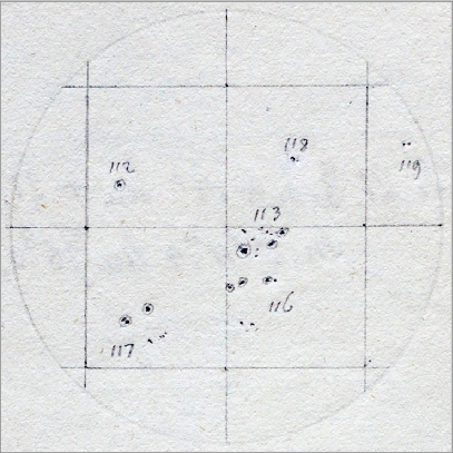
Figure 1: Example of the drawing style in the main period of 1831–1867. This full-disk drawing of 1847 July 22 shows spots with and without penumbrae. The drawing also shows two group designations (116 and 117) which actually refer to two individual groups each (see Sect. 3, also for the treatment of more difficult cases such as group 113).

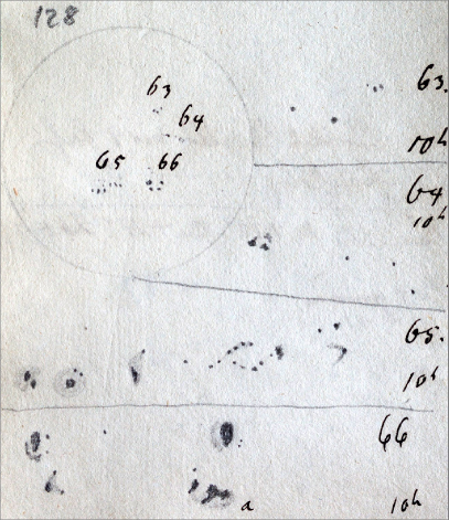
Figure 2: Example of the drawing style in the initial period of 1825–1830. This full-disk drawing of 1827 June 13 shows large spots which combine several umbrae and at least part of the penumbral area, as is revealed by the detailed drawings.

2 Calibration of sunspot areas

Apart from the importance to have reliable sunspot area information for the Schwabe period, we also need to know the individual sunspot areas for reasonable estimates of the two polarities and their locations in sunspot groups when determining the tilt angles of sunspot groups. The sunspot areas may be seen as proxies for the magnetic flux (e.g. Houtgast & van Sluiters 1948; Ringnes & Jensen 1960, for early studies), although the relation of the two may be complex, as emphasized recently by Tlatov & Pevtsov (2014).

Schwabe plotted the sunspots into relatively small circles of about 5 cm diameter, representing the solar disk. Given the finite width of a pencil tip, at least small spots must have been plotted with an area larger than a corresponding structure on the Sun would have at that scale. Pores, if plotted to scale, would need to have diameters of 0.04–0.1 mm in such a drawing. The umbral areas measured in the drawings therefore need to be converted into physical areas on the Sun.

There are two ways of obtaining physical sizes of the sunspots drawn by Schwabe. The one requires the existence of high-resolution drawings by other observers within the observing period of Schwabe for calibration. The other is a statistical approach using data sets of the 20th century to calibrate the sizes. We will first describe the latter method, since the number of high-resolution drawings by other observers that can be employed for the first method is very limited. The statistical approach also required a splitting of the data into two sets: 1825–1830 and 1831–1867. This is due to a change in the drawing style after 1831 Jan 1, as demonstrated in Figs. 1 and 2. In the initial period, Schwabe plotted spots without distinction of umbrae and penumbrae. In the second period starting in 1831, Schwabe distinguished umbrae from penumbrae. In those cases, umbral sizes were measured. We begin with the second period when areas are clearly umbral and describe afterwards a work-around for the conversion of sunspot sizes to umbral areas in the initial period until 1830.

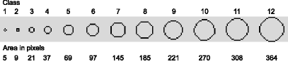
Figure 3: Twelve cursor shapes (size classes) used for the size estimates of the sunspots drawn by Schwabe. The bottom line gives the area in square pixels on the screen, including the black border pixels.

2.1 Indirect umbral areas for 1831–1867

One approach to obtaining physical areas of the sunspot sizes is of a statistical nature. Sunspots were divided into 12 classes by size, as introduced by Arlt et al. (2013). The measurements were actually carried out with twelve different circular cursor shapes having areas from 5 to 364 square pixels. Their shapes and screen areas are shown in Fig. 3. The classes increase monotonously in area, but were chosen relatively arbitrarily. Any more precise individual pixel-counts of umbral areas are unlikely to yield more accurate data, since the drawings are meant to be sketches of the sunspot distributions and sizes rather than exact copies. More details are given by Arlt et al. (2013).

The division into 12 size classes is done both for Schwabe’s dataset and for a modern data set (see below), whereby for the modern dataset the classes are chosen such that each class has the same relative number of sunspots as the corresponding class in Schwabe’s data. In other words, the relative abundances of the twelve size classes of the Schwabe spots are compared and calibrated with 20th century data by building histograms of 12 artificial size classes constructed to contain the identical abundances. The average umbral area in such an artificial class gives us the umbral area corresponding to a Schwabe size class. Finally, a function for the area depending on the heliocentric angle of a spot from the centre of the solar disk is fitted for each size class. We will refer to this angle as ‘disk-centre distance’ $\delta$ in the following.

The reference data sets used to obtain a statistical mapping of sunspot umbral areas are from photoheliographic data of the observatories of Debrecen, Mt. Wilson, Kodaikanal, and the MDI instrument of SOHO. As described by Győri (1998), an improved automatic analysis method was used for the Debrecen data starting in 1988. Before that, from 1974 to 1987, the areas were measured by video techniques (Dezső et al. 1987). In the 1974–1987 data, the area values of larger sunspots at disk-centre distances $\delta>60^{\circ}$ increase very rapidly with $\delta$. This effect is not seen in the area values measured from 1988 onward, so we have used the Debrecen data from 1988–2013 only. The Mt. Wilson data were analysed by Howard et al. (1984) and contain spot properties from 1917–1985. The Kodaikanal data covering 1906–1987 were obtained in almost the same way as the Mt. Wilson ones (Sivaraman et al. 1993). The MDI data for 1996–2010 were obtained using a telescope of 4 arc seconds resolution (Watson et al. 2011) which is similar to or perhaps a bit worse than the resolving capabilities of Schwabe’s setup. Note that the data from the Greenwich Photoheliographic Database were not used because it contains group area totals instead of areas of individual spots.

Typical diameters of solar pores in white light are between 1000 km and 4000 km (Keppens & Martínez Pillet 1996). That converts to $0.8$–$13\cdot 10^{6}$ km² or 0.26–4.1 millionths of the solar hemisphere (MSH). We are using a lower limit of 1 MSH for the construction of the histogram as argued below. In the Debrecen data, integer values of the projected area in millionths of the solar disk are given ($0,1,2,\dots$), while the corrected areas are given in MSH, also as integer values. Since the projection correction increases the area, whereas the conversion to MSH reduces the value by half, the lower limits of 1 in both quantities are therefore statistically compatible. We discarded all spots smaller than 1 MSH from the other data sets before the analysis. Ideally, one would want to define a minimum spot size plotted by Schwabe, but in reality, his drawing style was not that straight-forward. Whenever he detected a small group on the Sun, he indicated its location by small dots. In more complex groups, however, he did not indicate all the small spots because of their abundance. There is apparently no clear lower limit for the spot size. We therefore use a compromise at this point, excluding the smallest pores, and start from 1 MSH which is also the lower limit in the Debrecen data.

The relative abundances of the twelve cursor size classes, denoted by $i=1,2,\dots,12$, are determined for three different ranges of disk-centre distances, which were $\delta<30^{\circ}$, $30^{\circ}$–$60^{\circ}$, and $60^{\circ}$–$70^{\circ}$. These distance classes are numbered as $d=1,2,3$. The upper limit of $70^{\circ}$ is due to the fact that not all reference data sets contain spots beyond that distance. The four reference data sets (this number will be denoted by $N$ in the following) are now also divided into twelve classes fulfilling the same relative abundances as obtained for the Schwabe classes, again split into the three selected ranges of distances. The histograms are based on the umbral areas which are corrected for foreshortening. We therefore expect a mapping of size classes with a fairly small dependence on $\delta$.

Then the area for each cursor size is calculated by the unweighted average of all spots

$$\overline{A}_{id}={\sum\limits_{n=1}^{N}\sum\limits_{j=1}^{S_{\!nid}}A_{njid}}\left/{\sum\limits_{n=1}^{N}S_{\!nid}}\right.,$$ (1)

where $\overline{A}_{id}$ is the area for a cursor of $i$-th size class in the $d$-th disk-centre distance class, ${A_{njid}}$ is the umbral area (corrected for projection by $\cos^{-1}\delta$) of the $j$-th spot in the $n$-th data source, $i$-th size class and $d$-th distance class, and $S_{\!nid}$ is the total number of spots present in $n$-th data source, $i$-th size class in $d$-th distance class. Note that these averages consist of different histogram bins for different $n$. For example, the equivalent class-5 bin in the Debrecen data will have other area limits than the equivalent class-5 bin of the MDI data. The averaging helps smooth possible systematic over- or underestimations of areas in the 20th-century data sources. The averages $\overline{A}_{id}$ are not immediately areas corrected for foreshortening, since the histogram classes are constructed using Schwabe’s raw sunspot sizes. We will capture any possibly remaining disk-centre distance dependence in Sect. 2.4, where functions through the three distance classes for each $i$ will be derived, i.e. 12 functions for the 12 size classes.

2.2 Indirect umbral areas for 1825–1830

The sunspots in the early full-disk drawings from 1825 to 1830 were not drawn at a good resolution. Instead, Schwabe plotted high-resolution magnifications at unknown scale beside the full-disk drawings. The magnifications show that nearby spots were combined in the full-disk drawings. The spots in these drawings are therefore often ‘blobs’ made out of very close spots and including the penumbrae between those spots. Hence, the pencil dots used to measure the sizes of those spots do not represent their umbral area. To estimate the area for these spots, we need to compare the size statistics with grouped spots including penumbrae. To do that, we combined the spots inside a single penumbra in a modern data set and used these for the statistical estimation of the area.

Among the data used here, the Debrecen data is the only source which contains umbral and penumbral areas broken down into individual spots. Recently, Tlatov et al. (2014) published detailed measurements of the Kislovodsk Mountain Astronomical Station. Since those only cover the somewhat peculiar cycle 24, we prefer not to use them for the area calibration of Schwabe’s drawings. The conversion of the 1825–1830 data is therefore based on the Debrecen data (1988–2013) as a mixture of different cycles. From that source, we prepared a data set in which all the umbrae inside a continuous penumbra are added and considered as a single spot of which we store the whole-spot area and the total umbral area in each spot. Now we divide the whole-spot areas into 12 classes with the same relative abundances as we obtained from Schwabe’s 1825–1830 data, but use the corresponding umbral areas for an average according to Eq. (1) for each size class in each distance class. The results for the distance classes are again combined into a function of the disk-centre distance in Sect. 2.4.

There are still differences between these combined spots from the Debrecen data and the pre-1831 Schwabe spots. (1) A penumbra with a single umbra would look similar to a penumbra with two umbrae in Schwabe’s drawings. The penumbral area between the two umbrae in the latter case, however, will lead to different total umbral areas when derived from the Debrecen data. (2) It is not always the entire penumbra which Schwabe plotted in a ‘blob’. (3) All the umbrae inside a penumbra are added in the Debrecen data, even for very extended penumbrae. Schwabe, however, did not club together all the umbrae inside a connected penumbra when it was very large, but plotted ‘sub-penumbrae’ in that case.

There are 38 spots apparently drawn without the inclusion of a penumbra which were found from the visual comparison of disk drawings with magnifications. These spots were not used in the procedure described here; their areas were calculated using the method discussed in Sect. 2.1.

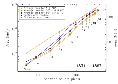
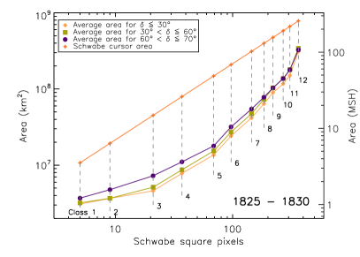
Figure 4: Average areas in km² (left ordinate) and MSH (right ordinate) for each of the twelve size classes (abscissa), and for three different centre-distance ranges: $<30^{\circ}$ (diamonds), $30^{\circ}$–$60^{\circ}$ (squares), and $60^{\circ}$–$70^{\circ}$ (circles). The areas corresponding to the simple pixel areas of the size classes without any calibration are indicated by plus signs. The direct calibration of size classes by observations from Sestini in 1850 are shown as triangles. Top: average areas for the data from 1831–1867. Bottom: average areas for the data from 1825–1830. An open symbol means that the number of spots used in the calculation of the average area is less than twenty. Note that the lower curves in the lower panel do not imply smaller areas, but they rather mean that any spot of a given true area were drawn as a spot of larger class in 1825–1830 than in 1831–1867.

2.3 Umbral areas from parallel observations

For a short period from 1850 Sep 19 to Nov 4, large-scale drawings are also available from Sestini who observed from Washington, D.C., comprising a total of 42 full-disk graphs (Sestini 1853). We compiled spots seen by both Schwabe and Sestini and measured the umbral areas of the corresponding spots in Sestini’s drawings. There were not enough observations to cover the whole range of size classes – we could only cover classes 1–6. We will come back to the results in the following Section. One has to note though that the time difference between the observations from Dessau and the ones from Washington implies changes in the evolution of the spots either leading to wrong areas or to wrong spot associations between the two observers.

2.4 Final mapping of sunspot sizes

Figure 4 shows the mappings of Schwabe size classes to physical areas in km² and MSH for three different ranges of disk-centre distances for the statistical conversion as well as a mapping for the calibration with concurrent high-resolution observations. One immediate result is that the direct conversion of the pencil spots in Schwabe’s drawings into sunspot areas would lead to overestimated umbral areas in most size classes. One can also see that the areas corresponding to the pixel areas do not form a linear function or power law. The areas from the comparison with the sunspots observed by Sestini in 1850 are in good agreement with the indirect mapping based on the size distribution. This shows that the direct conversion of pixel areas into sunspot areas is not a good choice. The only exception is class 5, but it contains only 21 measurements and may be a poor estimate (as is the one for class 6).

The lower panel of Fig. 4 appears to show much smaller areas. This is not true, however. The graph actually shows that a 5-MSH spot which was typically drawn as a class-3 dot in 1831–1867, was represented by a class-5 dot before that period, since it encompassed a considerable fraction of the penumbra at that time. The areas of class 3 in the top panel cannot be compared with the areas of class 3 in the lower panel. Sunspot sizes corresponding to large size classes were much more often used by Schwabe in the period of 1825–1830 than afterwards (note that there are no longer open symbols with fewer than twenty spots in the lower panel).

The dependence of final areas on the disk-centre distance is described by functions of the form

$${\cal A}_{i}(\delta)=a_{i}+\left(b_{i}/\cos\delta\right),$$ (2)

where $a_{i}$ and $b_{i}$ are coefficients for the $i$-th size class and $\delta$ is the distance of the spot from the centre of the solar disk. In the end, there are 12 functions for the period 1825–1830 and another 12 functions for the period 1831–1867. They deliver a mapping of the size classes into physical areas.

When computing the areas for the final sunspot data base, the area is not calculated if a spot distance is greater than $85^{\circ}$ from the disk centre, since the area values become very uncertain. All spots with $\delta\leq 70\degr$ are reliable in the sense that they are covered by the statistics leading to the mapping. All spots with $70\degr<\delta\leq 85\degr$ are uncertain because they rely on an extrapolation of the mapping, while all spots with $\delta>85\degr$ are highly uncertain and are therefore excluded from the data base. The smallest sunspot area occurring in our data after applying Eq. (2) is 1 MSH which is consistent with the initial lower limit for spots in the reference data sets.

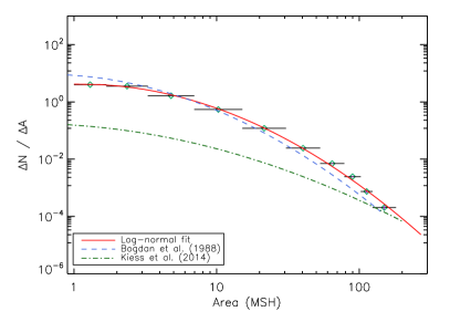
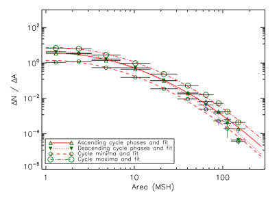
Figure 5: The distribution of estimated umbral areas of sunspots. Top: The area distribution for 1831–1867. The solid curve shows the log-normal fit. The dashed curve and dash dot curve are the fit curves form Bogdan et al. (1988) and Kiess et al. (2014), respectively. The horizontal bars show the widths of the bins. The error margins on the distribution values are all smaller than the symbols. Bottom: The area distribution of spots for ascending phases, descending phases, cycle minima and maxima of all cycles within 1831–1867. The lines show the log-normal fits for the corresponding area distributions.

2.5 Distribution of sunspot area

The data base of Schwabe’s observations contains a total of 135 921 entries comprising 134 386 spots with size estimates (each line corresponds to an individual umbra) as well as 1535 spotless days (each line corresponds to a day with zero spot size). Whenever we use the term ‘spots’ we refer to individual umbrae as far as Schwabe resolved them. Positions are not available for 849 umbrae because the orientation of the drawing could not be identified. No physical areas are available because $\delta$ is missing. There are another 41 umbrae beyond $85^{\circ}$ from the centre of the disk for which areas are not calculated because of too large uncertainties. The area values are therefore available for 133 496 umbrae. To study the distribution of areas, we consider the spots within $\pm 50^{\circ}$ central meridian distance (CMD) and within $\pm 45^{\circ}$ latitude. The same latitude limit was chosen by Bogdan et al. (1988). The central meridian limit, however, was $\pm 7\aas@@fstack{\circ}5$ in Bogdan et al. (1988) in order to avoid duplicate counts of groups (a group will typically appear only once in a $15\degr$ window because of the solar rotation). Since drawings by Schwabe are not available on all days, we need to widen this window reasonably and found $\pm 50^{\circ}$ a good compromise between not missing too many groups due to observing gaps on the one hand and the contamination by duplicate consideration of groups on the other hand. The latter will actually not affect the distribution significantly, since Baumann & Solanki (2005) and Kiess et al. (2014) did not see any drastic changes between counting umbrae only once and counting them on every day they were visible. The lowest area considered for the distribution is our lowest area, 1 MSH. The above criteria reduce the data to a sample of 104 217 spots in total, and 96 984 spots from 1831 to 1867.

The umbral area spectrum was obtained as described by Bogdan et al. (1988) with the exception that they used a lower umbral area limit of 1.5 MSH. Since the distribution is differential, the different lower limit should not affect the shape of the curve. The bins for small areas were selected such that each bin encompasses approximately one size class up to class 9, whereas one additional bin was defined such that it contains the spots from class 10 and about half the spots in class 11. All spots even larger than that ($\geq 185$ MSH) were outside the above mentioned CMD window. Dividing the area range into twenty bins as in Bogdan et al. (1988) would have caused a strong scatter since the Schwabe areas accumulate near twelve typical area values, because the dependences on the disk-centre distance described by (2) are all small.

The area distribution of the Schwabe spots also resembles a log-normal distribution and looks similar to the curve by Bogdan et al. (1988). The parameters for such a distribution over the area $A$ are obtained through a fit by the function

$$\ln\left(\frac{\mathrm{d}N}{\mathrm{d}A}\right)=-\frac{\left(\ln\leavevmode\nobreak\ A-\ln\leavevmode\nobreak\ \langle A\rangle\right)^{2}}{2\leavevmode\nobreak\ \ln\leavevmode\nobreak\ \sigma_{\!A}}+\ln\left(\frac{\mathrm{d}N}{\mathrm{d}A}\right)_{\rm max},$$ (3)

where $(\mathrm{d}N/\mathrm{d}A)_{\rm max}$ is the maximum of the area distribution function, $\langle A\rangle$ is the mean, and $\sigma_{\!A}$ is the geometric standard deviation. Table LABEL:fitparameters shows the log-normal fit parameters obtained with a Levenberg-Marquardt least-squares method. The cycle minima and maxima were taken from the “Average” column of the cycle timings by Hathaway (2010). Minima periods and maxima periods are defined as $\pm 1$ yr around the minima/maxima, while the ascending and descending phases are the remaining periods.

Table 1: Log-normal fit parameters for the Schwabe data and various subsets of them.

Data	Umbrae	$\langle A\rangle$	$\sigma_{\!A}$	$\left(\frac{\mathrm{d}N}{\mathrm{d}A}\right)_{\rm max}$
		[MSH]	[MSH]	[MSH-1]
All data (1825–1867)	104 217	1.05	3.8	3.8
1825–1830	7 233	0.58	9.9	1.7
1831–1867	96 984	1.10	3.5	4.2
Cycle 7	9 448	1.09	5.3	1.3
Cycle 8	22 382	1.08	3.8	4.0
Cycle 9	36 862	1.08	3.0	5.3
Cycle 10	35 181	1.10	3.4	4.9
Ascending phases	13 613	1.09	3.5	3.7
Descending phases	46 763	1.10	3.1	4.7
Cycle minima	3 507	1.08	3.4	1.4
Cycle maxima	31131	1.10	3.6	7.6

The top panel of Fig. 5 shows the resulting total area distribution of umbrae for 1831–1867. The errors on the ordinate values were estimated by $(\Delta N/\Delta A)/\sqrt{\Delta N}$, where $\Delta N/\Delta A$ is the discrete area distribution value and $\Delta N$ is the number of spots in each bin. The errors are all smaller than the symbols. The lower curve from Fig. 1 in Bogdan et al. (1988), which is the fit to the full range of umbral areas of 1.5–141 MSH, and the curve from Kiess et al. (2014) are also plotted in Fig. 5 for comparison. While the data of both analyses also influence our size calibration of Schwabe’s sunspots, the distribution only agrees with the one by Bogdan et al. (1988) based on Mt. Wilson data. Interestingly, also the area distributions obtained from group umbral areas (Baumann & Solanki 2005) agree fairly well with our results. The peak position $\langle A\rangle$ of their log-normal distribution from the Greenwich group data is ten times larger than ours from individual spot data, in good agreement with the fact that sunspot groups consist of roughly ten spots on average.

The bottom panel of Fig. 5 shows four individual area distributions for the ascending and descending phases of the cycles as well as for the cycle minima and maxima. They exhibit nearly the same distribution as the whole area distribution. The descending phases of all cycles have larger $(\mathrm{d}N/\mathrm{d}A)_{\rm max}$ than the ascending phases, however. The fairly small variation of $\sigma_{\!A}$ is remarkable and confirms the corresponding findings by Bogdan et al. (1988) and Schad & Penn (2010).

The umbral area distribution was calculated for the data from 1825–1830 and from 1831–1867 separately, and the fit parameters are given in Table LABEL:fitparameters. The distribution for the earlier period is much wider, with $\sigma_{\!A}$ being similar to the one by Kiess et al. (2014) who derived $\sigma_{\!A}=10.7$ ($\sigma=1.54$ in their work).

3 Group definitions

Tilt-angles of groups will be sensitive to the actual association of spots into groups. Schwabe’s original drawings contain group names which he started from number one every new year. His perception of a group was often too broad. A fair number of sunspot clusters actually contain two or more groups. This new definition of the groups was made by manual inspection of the drawings. We also used the evolutionary information of the clusters and sub-clusters provided by the images of adjacent days. Very often, a small apparently new bipolar group emerged near an existing one and showed its individual evolution through the Waldmeier (or Zurich) types. Schwabe included them in the group number of the existing group, while we defined a new group in many such cases. In other cases, when splitting of the polarities was not obvious and the parts of the group were all in the same evolutionary phase, we kept Schwabe’s definition, despite leading to somewhat large groups of $30\degr$ extent or more. Any splitting, however, would have been very arbitrary and would add noise rather than new information to the tilt angle data base. A total of 56 groups with extents $\geq 30\degr$ size remained.

Table 2: Statistics of coverage, spot areas, groups, and tilt angles $\alpha$ for Schwabe’s observations in 1825–1867. CMD is the central meridian distance of the area weighted centre of a group.

Period	Days with	Gaps longer	Gross groups	Unique groups	Groups	Group tilts with	Group tilts with
	drawings	than 5 days	with areas	with areas	with tilt	$|{\rm CMD}|<60\degr$	$|{\rm CMD}|<60\degr$
							and $\alpha>3\degr$
1825–1830	1187 (63.0%)	32	4 401	945	2 452	2 159	1 745
1831–1867	8808 (65.2%)	149	27 116	5903	20 689	17 365	13 803
Total	9995 (64.9%)	182	31 517	6848	23 141	19 524	15 548

Figure 6: The number of new groups obtained by splitting Schwabe’s original groups, normalised to the number of groups before splitting (i.e. Schwabe’s original groups). The criteria for splitting a group are described in the main text.

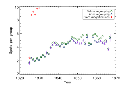
Figure 7: Annual averages of the number of spots per group calculated before regrouping of sunspot groups (circles), after regrouping (triangles), and manually counted number of spots from the magnification drawings of sunspot groups (diamonds). Uncertainties are only given for the values after regrouping and are obtained from the relative Poissonian error $1/\sqrt{n_{\rm counts}}$, where $n_{\rm counts}$ are the number of all instances of all groups in a given year (groups count several times with different numbers of spots).

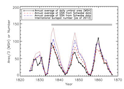
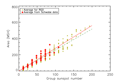
Figure 8: Top: Annual averages of total-disk umbral area of sunspots in MSH and divided by three (solid line), the group sunspot number (GSN) derived from our groupings (dashed line), the sunspot number (SSN; Wolf number) derived from our groupings and the actual number of spots in the full-disk drawings (dash-dotted line), and the official International Sunspot Number (dotted line) of before the revision suggested by Clette et al. (2014) which was not yet available. The gray horizontal bar indicates the period in which the number of spots per group was fairly constant (cf. Fig. 7). Bottom: Daily total umbral areas versus GSN (in case of Schwabe, the GSN is based on our grouping in Schwabe’s drawings, corresponding to the dashed line in the upper panel), averaged over 100 values in each group sunspot number bin for the Schwabe data (circles) and the Greenwich data (asterisks). The solid and dashed lines are linear fits through the Schwabe and Greenwich data, respectively, being enforced to go through the origin.

Figure 6 shows the ratio of the number of newly formed groups, i.e. those obtained by splitting Schwabe’s original groups, to the original number of groups. For instance, if there were a total of 10 groups which were all split into two, resulting in 10 new groups, the ratio would be one (100% splitting). The large fraction of splittings seen after 1850 is partly due to the presence of very many closely located groups, but chiefly due to a wider definition of groups Schwabe adopted during those cycles. In nine cases, Schwabe assigned one group designation each to two spots, while they apparently form one bipolar group. We combined those cases to one group name.

The splittings are marked by modified group names in the above mentioned data file. The two groups 116 and 117 in Fig. 1 will now appear as four groups, 116-0, 116-1, 117-0, and 117-1 in the catalogue. Combined groups are marked with plus signs in the new group name, e.g. 39+40.

To demonstrate the impact of the regrouping (splitting as well as combining), Fig. 7 shows the annual averages of the number of spots per group, derived from Schwabe’s group definitions and derived after regrouping by visual inspection. Additionally, the sunspot group magnifications drawn by Schwabe (see Fig. 2) were used to compute a third set of average spot numbers per group. Since the magnifications are not biased towards exceptionally large groups until 1830, we give only the averages for 1826–1830. These spot numbers per group obtained from detailed drawings of individual groups match modern values very well (Tlatov 2013; Clette et al. 2014). After 1830, only selected, big groups were magnified, so the values of spots per group are biased.

In the averages derived from the full-disk drawings, there is a significant increase in the number of spots per group from 1830 to 1836. This increase was not flattened after the regrouping of sunspot groups. It may be partly due to initially smaller true numbers of spots per group and partly due to the early, coarser drawing style of Schwabe. The most notable jump from 1835 to 1836 does not coincide, however, with the change in drawing style in 1830/1831. An increase in the number of spots per group can also be seen after the other minima, namely in 1843–1847, 1856–1858, and 1866–1867. Therefore, the change in drawing style and the recovery from the activity minimum in 1833 are probably superimposed effects.

By the same token, we may spot small peaks coinciding with the solar cycle maxima 8, 9, and 10 in Fig. 7. This effect has also been observed – even more drastically – by Clette et al. (2014) in 20th-century data, and it may actually be a mixture of a real effect and observational bias (basically because on a crowded Sun, the splitting of groups is difficult).

The upper panel of Fig. 8 shows the annual averages of umbral areas of sunspots. They are compared to the yearly averages of the group sunspot number (GSN) according to our own group number information and the (Wolf or Zurich) sunspot number (SSN), both derived from Schwabe’s observations, as well as to the International Sunspot Number (ISN). Good agreement is found between umbral areas and Schwabe’s group sunspot number for cycle 8, while the areas of cycles 7 and 9 fall below the (rescaled) sunspot numbers and cycle 10 has larger areas than the sunspot numbers indicate. Since Schwabe’s observing method, telescope and drawings are very constant after 1835, the difference between the ISN and the Schwabe record may be due to calibration issues of the ISN before 1849 (Leussu et al. 2013).

In an attempt to assess the correlation of the umbral areas with the group sunspot number, we plot averages of 100 daily all-disk umbral areas versus the corresponding group sunspot number of the same days in the lower panel of Fig. 8. The same was done for the Greenwich photoheliographic database which contains umbral areas until 1976. The graph is similar to the one by Balmaceda et al. (2009) who used the total spot areas instead. There is an intrinsic scatter in the correlation due to a certain randomness if both the sunspot number and sunspot areas are related to an internal magnetic field, rather than to each other. The uncertainty from the randomness has been reduced to about 10% by averaging over 100 days. Although the scatter in total umbral areas is higher than that due to randomness (as seen in the bottom panel of Fig. 8), it is comparable to the results from the Greenwich data, except for a slight tendency to larger areas (lines of linear fits through the origin were added for clarity in Fig. 8). We therefore conclude that the areas inferred from the Schwabe data are compatible with the Greenwich data, which did not enter our calibration at any step. The Schwabe areas do show, however, cycle-to-cycle variations in the strength of the correlation with the sunspot number indices.

The final total numbers of groups as well as the numbers of groups that will have tilt angles (see Sect. 4) are given in Table 2.

4 Tilt-angles of groups

4.1 Determination of tilt and separation

The tilt angle of a given sunspot group is calculated in a plane tangential to the solar surface in an estimated mid-point of that particular group to avoid problems with the curvilinear heliographic coordinates. The mid-point of the group (hereafter box-centre as opposed to the area-weighted centre of gravity of the group) is obtained using the easternmost and westernmost spots as well as the northernmost and southernmost spots of a given group. The longitude and latitude of the box-centre is set to be the contact point of the tangential plane with the solar surface. The Cartesian coordinates in this plane are $x_{i}$ and $y_{i}$ for the $i$-th spot and $x_{\rm g}$ and $y_{\rm g}$ for the box-centre and are normalised with respect to the solar diameter.

The algorithm then checks for the number of spots in a group. If it is equal to two, it proceeds to calculate directly the tilt angle and polarity separation. If it is more than two spots, we have to assess the most probable configuration of which spots belong to which polarity, since magnetic information is not available. We look for the most probable division of the group into two clusters by finding the least positional variance within the individual clusters. For that, we let a division line, running through the box-centre, rotate from $\theta=0$ to $\theta=180\degr$ and obtain – for each angle – a cluster of ‘leading’ spots and a cluster of ‘following’ spots. This is achieved by using a vector perpendicular to the division line, $\@vec{D}=\left(\cos\leavevmode\nobreak\ \theta,\sin\leavevmode\nobreak\ \theta\right)$. The sign of the inner product of this vector with the spot vector, $\@vec{S}_{i}=(x_{i}-x_{g},y_{i}-y_{g})$ defines the cluster (‘polarity’) membership of the $i$-th spot. The sum of the two variances of the spots’ coordinates on either side of the division line is calculated. We denote the angle at which the least positional variance is achieved by $\theta_{\rm opt}$ and adopt it as the most probable division of the sunspot group into polarities. The area-weighted centres of the polarities found are then calculated. The eastern and western parts correspond to the following and leading polarities, respectively, and their coordinate pairs are denoted by $(x_{\rm F},y_{\rm F})$ and $(x_{\rm L},y_{\rm L})$. The coordinate pairs convert to heliographic coordinates $(\phi_{\rm F},\lambda_{\rm F})$ and $(\phi_{\rm L},\lambda_{\rm L})$, respectively.

The tilt angle $\alpha$ is computed by

$$\tan\alpha=\left\{\begin{array}[]{l}\left(y_{\rm F}-y_{\rm L}\right)/\left(x_{\rm L}-x_{\rm F}\right)\qquad\mbox{if $\lambda_{\rm g}\geq 0$}\\ \left(y_{\rm L}-y_{\rm F}\right)/\left(x_{\rm L}-x_{\rm F}\right)\qquad\mbox{otherwise},\end{array}\right.$$ (4)

where $\lambda_{\rm g}$ is the heliographic latitude of the box-centre. The tilt angles are positive if the leading polarity is nearer to the equator. Note that these operations are done in a tangential plane through the box-centre. Problems with measuring on a spherical surface are thus very small. The tilt angles calculated are called ‘pseudo-tilt-angle’ as in case of the Mt. Wilson data because magnetic polarity information is not available (Howard 1991).

The polarity separation is then computed on the great circle (orthodrome) through the polarities:

$$\cos\Delta\beta=\sin\lambda_{\rm F}\sin\lambda_{\rm L}+\cos\lambda_{\rm F}\cos\lambda_{\rm L}\cos(\phi_{\rm F}-\phi_{\rm L}).$$ (5)

The tilt angles are calculated for all spot groups with two or more spots.

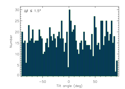
Figure 9: Histogram of the ‘tilt angles’ of supposedly unipolar groups in the Schwabe data, selected by a maximum ‘polarity’ separation of $\Delta\beta\leq 1\aas@@fstack{\circ}5$.

4.2 Sources of errors

Differences between various data sources and tilt angle determinations may have the following origins:

• unipolar groups are assigned a tilt angle erroneously,

• the method of computation may introduce a bias if the division angle through the bipolar group is presumed or prejudiced,

• ambiguity of the tilt angle sign due to the lack of magnetic information,

• or incorrect splittings or combinations of groups lead to spurious tilt angles.

The misidentification of unipolar regions generates a noise component whose distribution is much shallower than the distribution from bipolar groups (Wang et al. 2015; Baranyi 2015). The peak-to-tail ratio apparent from figure 8 in Wang et al. (2015) is about six for unipolar groups with $\Delta\beta<2\aas@@fstack{\circ}5$, while it is roughly 100 for the groups with $\Delta\beta>2\aas@@fstack{\circ}5$. In the Schwabe data, we find a peak-to-tail ratio of a bit more than two for $\Delta\beta<2\aas@@fstack{\circ}5$, while it is entirely uniform for $\Delta\beta\leq 1\aas@@fstack{\circ}5$ (Fig. 9). An interesting exercise is the determination of the dependence of the average tilt angle on the level of noise that is typically introduced by unipolar sunspot groups that are erroneously included when no magnetic information is available. We assume that the true tilt angle distribution is symmetric around its mean and denote it by $S(\alpha,\alpha_{0},\sigma_{\alpha})$, where $\alpha_{0}$ and $\sigma_{\alpha}$ are the true average and width of that distribution, respectively. We add the noise as a simple background constant $C$ which mimics the contamination by unipolar groups or other spurious tilt angles to simplify the analysis, giving an upper limit of the error introduced by those tilt angles. The average tilt angle is then

$$\langle\alpha\rangle=\int_{-\pi/2}^{\pi/2}\alpha\,(C+S)\,\mathrm{d}\alpha\,\left/\,\int_{-\pi/2}^{\pi/2}(C+S)\,\mathrm{d}\alpha\right..$$ (6)

We can replace the constant $C$ by the number of sunspot groups that contribute to $C$ as a fraction of the total number of groups and denote this fraction by $f$. We find

$$C=\frac{f\int_{-\pi/2}^{\pi/2}S\mathrm{d}\alpha}{\pi(1-f)}.$$ (7)

Inserting this into (6) leads to

$$\langle\alpha\rangle = (1-f)\int_{\pi/2}^{\pi/2}\alpha S\mathrm{d}\alpha\,\left/\,\int_{\pi/2}^{\pi/2}S\mathrm{d}\alpha\right.$$ (8)

$$\approx (1-f)\,\alpha_{0}.$$

The approximation coming from the finite-limit integral is better than $0\aas@@fstack{\circ}05$ up to $\alpha_{0}=42\degr$ for $\sigma_{\alpha}=20\degr$ and up to $15\degr$ for $\sigma_{\alpha}=30\degr$ – good enough for any relevant average tilt angles. The relation (8) tells us that if 10% of the individual tilt angles are spurious, the average tilt angle reduces by 10%, e.g. from a true value of $5\degr$ to a measured value of $4\aas@@fstack{\circ}5$. Looking at the cycle-to-cycle variations derived by Wang et al. (2015) for individual data sets, we infer cycle-to-cycle scatters (corrected by $t$-distribution) of 4%, 9%, and 14% for the Debrecen umbral-based tilt angles, the Debrecen whole-spot-based tilt angles, and the tilt angles from the Mt. Wilson white-light images, respectively. Since the cycle-to-cycle variations of the average tilt angles are that small, the possible contamination of the distribution should be assessed, especially when data from different sources are combined. Note that 100% noise naturally leads to an average tilt angle of $0\degr$ (without polarity information). The influence of unipolar groups can be reduced significantly by excluding all groups with apparent separations of $\Delta\beta<2\aas@@fstack{\circ}5$ or even $\Delta\beta<3\degr$ (Baranyi 2015).

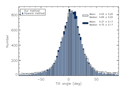
Figure 10: Histograms of the tilt angles in the Schwabe data, analysed with two different methods. Light bars show the excess of tilt angles from our isotropic method searching for the optimum polarity division, while dark bars show the excess of tilt angles from the method by Howard (1991). Only groups with area weighted centres within $\pm 60\degr$ CMD and polarity separations $\Delta\beta>3\degr$ are used.

We tried to further reduce the influence of spurious tilt angles by looking at the scatter of tilt angles of a given group during its evolution over several days. We denote the individual appearances of a group over several days as “instances”. A similar procedure was proposed by Li & Ulrich (2012). On the one hand, outliers due to ill-defined groups need to be removed. On the other hand, groups become unipolar at the end of their lifetime, but are still large and accompanied by pores, mimicking $\Delta\beta>3\degr$. We therefore determine the median tilt angle $\bar{\alpha}$ from the various instances of a given group and determine the average deviation from it by

$$\Delta\alpha=\sum_{i=1}^{I}|\alpha_{i}-\bar{\alpha}|/I,$$ (9)

where $I$ is the number of instances of the group and $\alpha_{i}$ are the tilt angles of the individual instances of the group. The tilt angle will be fairly reliable if the polarity separation is large. We therefore tested whether the tilt angle at maximum polarity separation, $\alpha_{\rm maxsep}$, does not deviate from the median significantly, using the criterion $|\alpha_{\rm maxsep}-\bar{\alpha}|<\Delta\alpha$. The groups fulfilling this criterion are a good guess of the ‘real’ bipolar groups, while others are omitted entirely. Now, within the accepted groups, all instances with $|\alpha_{i}-\bar{\alpha}|>2\Delta\alpha$ are omitted as outliers. A group turning unipolar near the end of its lifetime still exhibits scattered spots and pores around the remaining (large-area) polarity which will cause quickly changing spurious tilt-angles. Those (mostly H-type) groups are not supposed to deliver a tilt angle. We will call those cases ‘evolutionary outliers’ in the following.

The removal of ‘evolutionary outliers’ also requires the decision on which hemisphere a given group lay, since low-latitude groups may have instances on both sides of the equator, leading to jumps in the tilt angle. We decided upon the hemispheric ‘membership’ by the average (signed) latitude of the group instances of each group. The signs of the tilt angles of all instances are then computed assuming the single hemisphere obtained from that average latitude, regardless of the actual hemisphere of an individual instance.

With respect to the method of computing tilt angles, we used the Schwabe data set to compare the method by Howard et al. (1984) with our method. The former divides groups always with a north–south line leading to a bias with an avoidance of tilt angles near $90\degr$. Our method of trying all possible dividing lines is isotropic with equal prior probabilities for tilt angles of $90\degr$, $0\degr$, and $-90\degr$. Figure 10 shows a comparison of the two methods based on the Schwabe data of individual spots. The method of Howard (1991) tends to concentrate tilt angles at lower values.

Groups which are ‘reversed dipoles’ as compared to the typical polarity of a given cycle (anti-Hale groups) cannot be detected in white-light images or sunspot drawings. The anti-Hale fraction of all groups is about 8% (Li & Ulrich 2012; McClintock et al. 2014) or about 5% (Sokoloff & Khlystova 2010) or even lower (Sokoloff et al. 2015), based on magnetogram data. This fraction holds true for large bipolar regions though, while the fraction may be as high as 50% for ephemeral regions with areas less than 50 MSH (Illarionov et al. 2015), which are not relevant here as they are not accompanied by sunspots. In our cleanest distribution without ‘evolutionary outliers’, 95% of the groups are larger than 10 MSH in terms of their umbral group area. This translates to roughly 100 MSH total group area. For this lower limit of group areas, Illarionov et al. (2015) give an anti-Hale fraction of about 37%, while for large groups with 500 MSH or more, that fraction is 10% or less. The unsigned tilt angle distribution of anti-Hale groups is broader than that of the Hale groups, but with similar peaks (McClintock et al. 2014). The influence of the missing knowledge of the polarity on the average tilt angle is therefore relatively mild and not as strong as a similar fraction of random noise in the data.

The definition of what exactly is a group yields another source of possible errors. Baranyi (2015) revisited the Mt. Wilson and Kodaikanal data sets and compared them with Debrecen tilt angles. Among other things, she found that the automated routine used in the original analysis of the Mt. Wilson and Kodaikanal data often splits true groups into two smaller ones. While the average tilt angle by Howard (1991) ($4\aas@@fstack{\circ}2\pm 0\aas@@fstack{\circ}2$) was reproduced as $4\aas@@fstack{\circ}16\pm 0.19$, a higher value of $4\aas@@fstack{\circ}69\pm 0\aas@@fstack{\circ}20$ was found for 1917–1976 when these extra splittings were corrected. In terms of Eq. 9, this new value indicates a random noise fraction in the original value of 11%. That period of 1917–1976 is the one for which the Greenwich Photoheliographic Database was used as a reference to define proper groups. For 1974–1985, the Debrecen Photoheliographic Database was used to obtain the ‘true groups’, to give the average of $5\aas@@fstack{\circ}00\pm 0\aas@@fstack{\circ}47$. Note that the difference to $4\aas@@fstack{\circ}69\pm 0\aas@@fstack{\circ}20$ may actually be real and due to the different cycles covered.

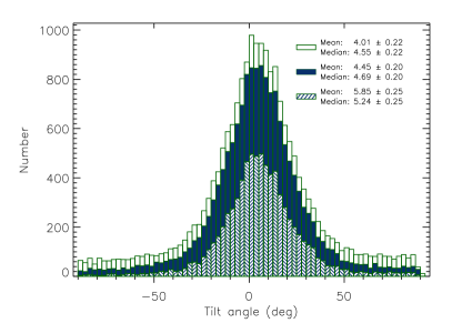
Figure 11: Histograms of the tilt angles of groups with area weighted centres within $60\degr$ central meridian distance. Open bars: entire set, filled bars: groups with a minimum polarity separation of $\Delta\beta_{\rm min}=3\degr$, and hatched bars: groups with $\Delta\beta_{\rm min}=3\degr$ and a removal of ‘evolutionary’ outliers that occur in the sequence of tilt angles during the evolution of any given group. This hatched histogram is an attempt to further reduce the influence of occasional unipolar instances of otherwise bipolar groups. See text for the detailed algorithm. The bin width is $2\aas@@fstack{\circ}5$.

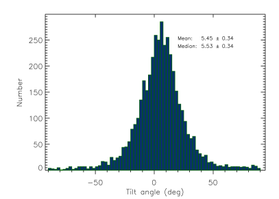
Figure 12: Tilt angle histogram of the Schwabe data for group centres within $60\degr$ central meridian distance and polarity separations $\Delta\beta>3\degr$. In this analysis, only spots with umbral areas of 5 MSH or more were used to compute the weighted positions of the polarities. The selection therefore affects both tilt angles and polarity separations. As compared with the hatched bars in Fig. 11, many groups have now turned into unipolar groups, since one of the polarities was represented by a single spot of less than 5 MSH.

4.3 Distribution and averages

Figure 11 shows the resulting distribution of tilt angles. Being quite broad, the distribution has its maximum at small, non-zero $\alpha$. Note that the open bars may include tilt angles which are erroneously computed for two or more spots of a single polarity, fragmented spots, and spots inside the same penumbra. The filled histogram therefore shows the distribution of tilt angles with polarity separations $\Delta\beta>3\degr$. In this distribution, spots inside a common penumbra are essentially excluded, but, on the one hand, true bipolar groups with very small polarity separations may also be excluded. On the other hand, spurious tilt angles due to a decaying big group with a single polarity may still contribute to this distribution, but are a very minor fraction (Baranyi 2015). The selection of bipolar groups may perhaps be fine-tuned by using an area-dependent minimum polarity separation, but we did not wish to impose biases which may affect the distribution of polarity separations. A constant minimum separation $\Delta\beta_{\rm min}$ is therefore used for selecting actual bipolar groups.

The average tilt angle for the distribution with $\Delta\beta_{\rm min}=3\degr$ and with area weighted group centres within $\pm 60\degr$ CMD is $4\aas@@fstack{\circ}45\pm 0\aas@@fstack{\circ}20$ (median $4\aas@@fstack{\circ}69\pm 0\aas@@fstack{\circ}20$) where the error of the mean is computed by the standard deviation of the distribution divided by the square root of the number of points, $\sigma_{\rm tilt}/\sqrt{n}$. For comparison, we may also compute the average tilt angle for $\Delta\beta_{\rm min}=0$ (again $|{\rm CMD|}<60\degr$) and obtain $4\aas@@fstack{\circ}01\pm 0\aas@@fstack{\circ}22$ (median $4\aas@@fstack{\circ}55\pm 0\aas@@fstack{\circ}22$). The lower value is consistent with our earlier supposition that spurious bipolarities add a certain amount of randomness to the data, bringing the average closer to zero. This average agrees relatively well with the ones found by Howard (1991) ($4\aas@@fstack{\circ}2\pm 0\aas@@fstack{\circ}2$) and Dasi-Espuig et al. (2010) ($4\aas@@fstack{\circ}25\pm 0\aas@@fstack{\circ}18$ for Mt. Wilson and $4\aas@@fstack{\circ}51\pm 0\aas@@fstack{\circ}18$ for Kodaikanal) for solar cycles 15–21 which were all computed without a lower limit, i.e. $\Delta\beta_{\rm min}=0$.

An analysis of the Debrecen data by Baranyi (2015) with careful extraction of truly bipolar groups delivered $5\aas@@fstack{\circ}12\pm 0\aas@@fstack{\circ}46$ for 1974–1985 (end of cycle 20 and cycle 21). Based on a minimum polarity separation of $\Delta\beta_{\rm min}=3\degr$, we recomputed the Mt. Wilson and Kodaikanal averages as well which resulted in values of $5\aas@@fstack{\circ}95\pm 0\aas@@fstack{\circ}42$ and $6\aas@@fstack{\circ}91\pm 0\aas@@fstack{\circ}45$, respectively, for cycle 21. Ivanov (2012) used the Pulkovo database (Catalogue of Solar Activity – CSA) for tilt angles in the period 1948–1991. We used their database and obtained an average tilt angle of $6\aas@@fstack{\circ}41\pm 0\aas@@fstack{\circ}14$ for cycle 21 only. In this sample, the groups were determined manually and contain a fairly clean definition of what a group is, similar to our analysis of the Schwabe drawings. Since the average tilt angle varies from one cycle to the next, we cannot compare Schwabe’s tilt angles with 20th-century ones directly, but we find that averages of clean tilt angle samples are typically $5\degr$ or larger.

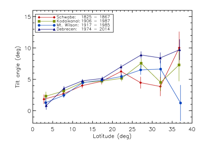
Figure 13: Dependence of the average tilt angle on the unsigned latitude for the data from Schwabe, Kodaikanal, Mt. Wilson, and Debrecen. Only groups with central meridian distances within $\pm 60\degr$ are used as the simplest common filter for all datasets. Errors of the means are the standard deviation of the bin sample divided by $\sqrt{n}$ in each bin.

The resulting histogram of tilt angles with deleted ‘evolutionary outliers’ (Sect. 4.2) is shown in Fig. 11 as hatched bars. The average tilt angle has risen to $5\aas@@fstack{\circ}85\pm 0\aas@@fstack{\circ}25$, based on 7765 tilt angles. We consider this the cleanest sample of tilt angles for cycles 7–10. The only average this value can be compared with now (as far as different cycles can be compared at all) is the one given by Baranyi (2015) where bipolar groups have also been selected fairly rigorously. However, that Debrecen tilt angle of $5\aas@@fstack{\circ}12$ is different in that spots smaller than 5 MSH are considered as pores which do not enter the determination of tilt angles and polarity separations. Figure 12 shows the histogram of the tilt angles restricted to spots that have areas $\geq 5$ MSH. The average of $5\aas@@fstack{\circ}45\pm 0\aas@@fstack{\circ}34$ (based on 4154 tilt angles) is slightly lower than the above value of $5\aas@@fstack{\circ}85\pm 0\aas@@fstack{\circ}25$, but not significantly. Even though the pores seem to play a minor role in determining reliable tilt angles, the difference shows that the minimum umbral area needs to be considered when combining several data sets.

Table 3: Modified format of the data of individual sunspots observed by Samuel Heinrich Schwabe. The format extends the one by Arlt et al. (2013) after column 93. In the Format column, I denotes integer fields, C8 is an 8-character text field, and, e.g., F5.1 denotes a 5-character-wide floating point field with one decimal. Areas in UMB are based on the derivation by (2).

Field	Column	Format	Explanation
YYYY	1–4	I4	Year
MM	6–7	I2	Month
DD	9–10	I2	Day referring to the German civil calendar running from midnight to midnight
HH	12–13	I2	Hour, times are mean local time in Dessau, Germany
MI	15–16	I2	Minute, typically accurate to 15 minutes
T	18	I1	Indicates how accurate the time is. Timeflag = 0 means the time has been inferred by the measurer (in most cases to be 12h local time); Timeflag = 1 means the time is as given by the observer
L0	20–24	F5.1	Heliographic longitude of apparent disk centre seen from Dessau
B0	26–30	F5.1	Heliographic latitude of apparent disk centre seen from Dessau
CMD	32–36	F5.1	Central meridian distance, difference in longitude from disk centre; contains –.- if line indicates spotless day; contains NaN if position of spot could not be measured.
LLL.L	38–42	F5.1	Heliographic longitude in the Carrington rotation frame; contains –.- if line indicates spotless day; contains NaN if position of spot could not be measured.
BBB.B	44–48	F5.1	Heliographic latitude, southern latitudes are negative; contains –.- if line indicates spotless day; contains NaN if position of spot could not be measured.
M	50	C1	Method of determining the orientation. ‘C’: horizontal pencil line parallel to celestial equator; ‘H’: book aligned with azimuth-elevation; ‘Q’: rotational matching with other drawings (spot used for the matching have ${\rm ModelLong}\neq{\rm`-.-^{\prime}}$, ${\rm ModelLat}\neq{\rm`-.-^{\prime}}$, and ${\rm Sigma}\neq{\rm`-.-^{\prime}}$).
Q	52	I1	Subjective quality, all observations with coordinate system drawn by Schwabe get Quality = 1. Positions derived from rotational matching may also obtain Quality = 2 or 3, if the probability distributions fixing the position angle of the drawing were not very sharp, or broad and asymmetric, respectively. Spotless days have Quality = 0; spots for which no position could be derived, but which have sizes, get Quality = 4.
SS	54–55	I2	Size estimate in 12 classes running from 1 to 12; a spotless day is indicated by 0
GROUP	57–64	C8	Group designation based on Schwabe, but modified by our regrouping
MEASURER	66–75	C10	Last name of person who obtained position
MOD_L	77–81	F5.1	Model longitude from rotational matching (only spots used for the matching have this)
MOD_B	83–87	F5.1	Model latitude from rotational matching (only spots used for the matching have this)
SIGMA	89–93	F6.3	Total residual of model positions compared with measurements of reference spots in rotational matching (only spots used for the matching have this). Holds for entire day.
DELTA	96–99	F4.1	Heliocentric angle between the spot and the apparent disk centre in degrees (disk-centre distance); it is $-.-$ for spotless days, while it is NaN if the spot position could not be determined.
UMB	100–103	I3	Inferred umbral area in millionths of the solar hemisphere (MSH); it is 0 for spotless days and NaN if spot position could not be derived or ${\tt DELTA}>85\degr$
A	105	C1	Flag saying whether area mapping is based on umbral (‘U’) or penumbral (‘!’) areas with the latter being less certain. Note that the actual area given in UMB is always umbral. Spotless days have $-$.

Table 4: Format for the tilt angle data derived from the sunspot groups observed by Schwabe, with format symbols as in Table 3. All areas are based on the UMB column in Table 3.

Field	Column		Format	Explanation
YYYY	1–	4	I4	Year
MM	6–	7	I2	Month
DD	9–	10	I2	Day
HH	12–	13	I2	Hour
MI	15–	16	I2	Minute; mean local time in Dessau, Germany
GROUP	18–	25	C8	Group name based on Schwabe, but modified by our regrouping
SP	27–	28	I2	Number of spots in a group
ARA	30–	32	I3	Sum of umbral area of all spots in a group, in millionths of the solar hemisphere (MSH)
AWL.L	34–	38	F5.1	Area-weighted heliographic longitude of the group
AWB.B	40–	44	F5.1	Area-weighted heliographic latitude of the group
TILTAN	46–	51	F6.2	Tilt angle of the group; positive sign means leading polarity closer to equator in either hemisphere. This tilt angle was found using an isotropic search for the most likely dividing line between the polarities.
TILTHO	53–	58	F6.2	Tilt angle computed as in Howard (1991) for compatibility reasons. It is based on a fixed vertical dividing line between the polarities and an approximative formula for the tilt angle.
POLSP	60–	64	F5.2	Polarity separation of the group in degrees on the solar sphere. This and the following items are based on the polarity definition for TILTAN.
FN	66–	67	I2	Number of spots in the following polarity
LN	69–	70	I2	Number of spots in the leading polarity
FAR	72–	74	I3	Umbral area of the following polarity, in MSH
LAR	76–	78	I3	Umbral area of the leading polarity, in MSH
FLL.L	80–	84	F5.1	Area-weighted longitude of the following polarity
FBB.B	86–	90	F5.1	Area-weighted latitude of the following polarity
LLL.L	92–	96	F5.1	Area-weighted longitude of the leading polarity
LBB.B	98–	102	F5.1	Area-weighted latitude of the leading polarity
GFC	104–	108	F5.1	Heliocentric distance of the group from the disk centre in degrees

The average dependence of the tilt angle on the absolute heliographic latitude (Joy’s law) is shown in Fig. 13. Together with the Schwabe data, we also plotted the average tilt angles obtained from the Mt. Wilson, Kodaikanal, and Debrecen data, using only tilt angles from groups within $\pm 60\degr$ CMD. The latitudinal dependence in the Schwabe data may be a bit shallower than the dependences from the other data sets – especially since it exhibits a non-zero intersection with the ordinate –, but is in agreement with them considering the uncertainty margins.

The format of the database containing the individual umbrae including umbral areas as well as spotless days is given in Table 3 which extends the one given by Arlt et al. (2013), while the format of the final data set containing the tilt angles and polarity separations of sunspot groups is given in Table LABEL:tilt_tab_format. Note that we give both, the tilt angles obtained according to our method described above as well as the tilt angles derived with the method by Howard (1991) in the latter table.

5 Summary

This study aims at determining physical areas of sunspots from drawings by Samuel Heinrich Schwabe in 1825–1867 as well as ordering these sunspots into (hopefully bipolar) groups and computing tilt angles of these sunspot groups for that period. The fraction of the solar disk covered by the pencil dots in the drawings cannot be directly converted into an area in km² or millionths of a solar hemisphere (MSH). We therefore constructed a mapping of the twelve arbitrary cursor sizes which were used by Arlt et al. (2013) to estimate the sizes of sunspots in the Schwabe drawings. For cycles 8–10, we obtain an average umbral area per day of 113. The Debrecen data for cycles 21–23, which were predominantly used for calibration, yield an average of roughly 150. The difference appears to be compatible with the stronger cycles in the second half of the 20th century and the fact, that Schwabe may have overlooked (or not plotted) a number of small spots. The umbral areas in the Greenwich Photoheliographic Database lead to an average of about 140 from cycles 12–20 of mixed strengths. Our area conversion is independent of the Greenwich data, but seems to agree with it fairly well, again taking into account that the Schwabe drawings may miss a few smaller spots.

The area distribution of the Schwabe sunspots exhibits a log-normal distribution in agreement with 20th-century data (Bogdan et al. 1988) and is essentially independent of the cycle phase. Schwabe’s original sunspot group designations were modified so that the groups comply with the modern understanding of a sunspot group, with the limitation of missing magnetic information. Using the positions and areas of all individual sunspots, the tilt angles as well as the polarity separations of the sunspot groups were calculated. Without the magnetic information, the definition of the polarities may lead to wrong associations affecting both tilt angles and polarity separations. The manual inspection of the groups before computing these quantities reduces these incorrect polarities as compared to fully automatic analysis schemes. Nevertheless, a remaining random component in the tilt angle distribution is likely to be present.

Both an updated sunspot database and a tilt angle database are available at http://www.aip.de/Members/rarlt/sunspots for further study. We note that in the sunspot database:

• sunspot areas for spots with ${\rm CMD}\leq 70\degr$ are reliable,

• sunspot areas for spots with $70\degr<{\rm CMD}\leq 85\degr$ are uncertain because they are an extrapolation of the statistical method employed,

• sunspot areas for spots with ${\rm CMD}>85\degr$ have been omitted,

• sunspot areas are calibrated using 20th century data; they will not serve for the purpose of detecting differences in areas between the 19th and the 20th century.

In the tilt angle database:

• tilt angles for all groups with two or more spots are reported,

• tilt angles for groups with ${\rm CMD}\leq 60\degr$ are considered reliable as the positions are reliable,

• tilt angles for polarity separations $\Delta\beta>3\degr$ (POLSP) are likely to be bipolar groups and should be selected for further analysis.

• the influence of spurious tilt angles from remaining unipolar groups can be further reduced by removing outliers from the sequence of tilt angles provided by the evolution of a given group. In brief, we removed days of appearance of a given group if the obtained tilt angle deviates significantly from the mean tilt angle of all appearances of that single group. The actual procedure is a bit more involved and is described in Sect. 4.2.

Joy’s law was found to be obeyed by the likely bipolar groups. The latitude dependence averages over all Schwabe cycles is not significantly different from cycles in the 20th century.

The applicability of white-light images for inferring cycle properties was doubted by Wang et al. (2015), mostly because of the inevitable contamination by actual unipolar groups. We believe the white-light images and drawings can still be useful, because (a) improved algorithms and visual inspection can reduce the impact of unipolar groups significantly, and because (b) we are interested in relative variations of tilt angles from one cycle to another, so consistently analysed sunspot data can still provide useful relative information of cycle-to-cycle variability. Care has to be taken that all data used for a particular study are consistent with each other, e.g. tilt angles from white-light images and magnetograms cannot be combined directly into a single record.

We have not studied the tilt angles of the individual cycles in this Paper. This will be the subject of a future study of tilt angles and strengths of invidual cycles as well as correlations thereof, extending ealier works on Mt. Wilson and Kodaikanal data. Especially cycle 7 is an interesting candidate for peculiarities, since it occurred shortly after the Dalton minimum (roughly 1795–1820). The current Paper aims at the disemination of the areas and tilt angles as the basis for further studies.