Supernovae as cosmological probes

Foreword

This work started as a wild goose chase for evidence beyond any doubt that supernova data show cosmic acceleration. Through a study involving artificial neural networks, trying to find parametrisation free constraints on the expansion history of the universe, we ran into trouble that led us all the way to reconsider the standard method. We encountered the same problem that has been lurking in many previous studies, only in an uncommon disguise. Solving this problem for the neural networks degenerated into solving the original problem. Having done that, it turned out that this result in itself is interesting. This thesis is more or less laying out the article [1] in all gory details.

The level of rigour throughout is kept, I think, sufficient but not over the top — particularly the chapter on statistics suffers at the hands of a physicist. I have tried to keep unnecessary details out of the way in favor of results and physical insight. I leave the details to be filled in by smarter people — well, more interested people.

A bunch of humble thanks to everyone who helped me at the institute, including — but presumably not limited to — Laure, Andy, Chris, Anne Mette, Sebastian, Assaf, Morten, Jenny, Christian, Tristan, and the rest of the Academy and high energy groups, and of course Helle and Anette without whom our building would crumble.

Thanks to Alberto and Subir for company and supervision on this trip through cosmology and data analysis. Obviously I extend my gratitude to Subir for teaching me the most valuable lesson leading to this work: don’t believe any analysis you can’t understand and, if time permits, carry out the analysis yourself. The following is my attempt at understanding the analysis of supernova data.

Abstract

The cosmological standard model at present is widely accepted as containing mainly things we do not understand. In particular the appearance of a Cosmological Constant, or dark energy, is puzzling. This was first inferred from the Hubble diagram of a low number of Type Ia supernovae, and later corroborated by complementary cosmological probes.

Today, a much larger collection of supernovae is available, and here I perform a rigorous statistical analysis of this dataset. Taking into account how the supernovae are calibrated to be standard candles, we run into some subtleties in the analysis. To our surprise, this new dataset — about an order of bigger than the size of the original dataset — shows, under standard assumptions, only mild evidence of an accelerated universe.

Contents

1. 1 Introduction
2. 2 Statistics
   1. 2.1 Probabilities
   2. 2.2 Expectations
   3. 2.3 Common distributions
   4. 2.4 Parameter estimation
   5. 2.5 Monte Carlo methods
   6. 2.6 Bayesian statistics
3. 3 Cosmology
   1. 3.1 General relativity
   2. 3.2 The cosmological principle
   3. 3.3 Cosmography
   4. 3.4 The Cosmological Constant
   5. 3.5 Alternative views
4. 4 Supernovae
   1. 4.1 Supernova progenitors
   2. 4.2 Observing supernovae
   3. 4.3 Comparison with the cosmos
5. 5 Putting the pieces together
   1. 5.1 The dataset
   2. 5.2 A statistical model of calibrated standard candles
   3. 5.3 Results of the main fit
   4. 5.4 Older analyses
6. 6 Conclusion

Introduction

The present standard model of cosmology explains quite well a host of observations. The inclusion of a cosmological constant in Einstein’s equations combined with the assumed homogeneous and isotropic Friedmann-Robertson-Walker metric description of spacetime gives us the hailed $\Lambda$CDM model. $\Lambda$ for the inferred cosmological constant, more popularly known as dark energy, and CDM is the cold dark matter. Dark because we can’t see it, and cold because apparently it behaves like non-relativistic particles — compared to (almost) massless particles, like neutrinos, which are hot. The baryonic matter is a minor component of the content of the universe.

The usual starting point of the history of modern cosmology is the two groups studying supernovae at the end of the nineties, [2, 3]. With observations of very far-away supernovae, the two teams independently claimed that the Hubble expansion rate is accelerating and inferred from that a best-fit universe with a cosmological constant density parameter around $0.7$. These results followed a massive experimental effort to find, classify, and calibrate the supernovae.

The big bang picture of the universe had emerged long before then. From extrapolating the expansion of the universe back in time, it was realised that in the past, the universe will have been much denser and much hotter. Two consequences of this is the cosmic microwave background (CMB) and a particular abundance of light elements, in particular ⁴He, in the early universe — which is of course altered during the history of the universe. Both these phenomenas are observable today, and confirm to a high degree this picture of a hot plasma filling the universe. Since Penzias and Wilson first saw a glimpse of the cosmic radiation, many experiments have come to the same conclusion. The three latest spaceborne missions, COBE, WMAP, and Planck, have, one after the other, measured to unprecedented precision the spectrum, and lately there has been a spur of interest in detecting gravitational waves in the hopes of information about the inflationary stage — even before the hot plasma!

Since mid-2000, another probe has also come into light. Baryon accoustic oscillations (BAO) are the remnant effects of soundwaves in the primeval plasma, which are supposed to enhance the matter correlation function at a particular scale — even in the late universe. Other constraints on the model come from more sides than I can hope to do justice here. Large scale structure surveys, gravitational lensing surveys etc., all help to constrain parameters of the model. Supernova observations have since the late nineties been one of the major players in cosmology. They, along with BAO and CMB observations are now the three major pillars of any analysis — an analysis of one will usually include the constraints of the others when quoting final results. Amazingly, these three observables apparently agree that the universe is indeed mostly cosmological constant and cold dark matter.

In the following I focus on the analysis of supernovae, in particular by performing a maximum likelihood analysis to put constraints on the cosmological model parameters. On the way, we will look at some of the problems of the standard model of cosmology and the standard treatment of the supernova data. I hope to have made the whole thing reasonably self contained.

I first present all the needed statistical tools in Chap. 2. This is followed by a description of the cosmology we will look at in Chap. 3 and the observations of supernovae in Chap. 4. Finally a presentation of the main analysis and result is in Chap. 5 and some concluding remarks in Chap. 6.

Statistics

Statistics is an old, well studied subject, from which physicists take that everything is distributed as gaussians and counting experiments have Poisson statistics. In the present section I hope to clarify why this is the case, and to which extent it is true. The main approach will be what is now known as frequentist, but Bayesian statistics will also be described briefly. For a vivid discussion of the differences between the two, see eg. [5].

2.1   Probabilities

I will start with the basics. We write the probability for some event, call it $A$, to happen $P(A)$. One immediate statement is that the universe is unitary, which is to say that something must happen, so the sum of all probabilities must be one: $\sum_{A}P(A)=1$. If the outcome $A$ is dependent on some other observation $B$, we write the probability of $A$ to happen, given $B$ as $P(A|B)$. This quantity is in general different from $P(A)$. We can connect the two through summing over the possible outcomes of the event $B$,

$$P(A)=\sum_{B}P(A|B)P(B)$$ (2.1.1)

We may also consider the joint probability of both events $A$ and $B$ to happen, $P(AB)$. We may now expand this as the probability of just one of the events happening times the probability of the other happening — given the other. In equations,

$$P(AB)=P(A|B)P(B)=P(B|A)P(A)$$ (2.1.2)

The second step follows from the symmetry of $A$ and $B$. The second equality is known as Bayes’ theorem. This is what underlies Bayesian statistics — but it is certainly true whether one is Bayesian or not.

If we wish to describe outcomes which are not discrete (like heads or tails) but rather continuous, we want to consider instead of just probabilities, a probability density function (pdf). To motivate this, consider an infinite number of possible outcomes of an experiment. Then the probability for any individual outcome in general vanishes. This is what the pdf sorts out for us. Say $A$ is a real number we are trying to predict. Then the pdf $f(A)$ is defined to fulfil

$$P(A\in[A_{min},A_{max}])=\int_{A_{min}}^{A_{max}}f(A)dA$$ (2.1.3)

This definition is trivially extended to multiple dimensions by simply extending $A$ and generalising the interval. We may write, generally

$$P(A\in\Omega)=\int_{\Omega}f(A)dA,$$ (2.1.4)

where $\Omega$ is some volume in the space of possible $A$s. As before, the integral over all possible outcomes must be $1$ by unitarity. We note that by putting in delta functions in the above pdfs, we can go back to the discrete picture. Say there are only discrete outcomes $A_{i}$ of $A$ with probabilities $p_{i}$, respectively. I can then write the pdf as

$$f(A)=\sum_{i}\delta(A-A_{i})p_{i}$$ (2.1.5)

What shall interest us most here are continuous distributions, ie. pdfs. The Eqs. (2.1.1)-(2.1.2) extend to

$$f(A)= \int f(A|B)f(B)\ dB$$ (2.1.6)

$$f(A|B)f(B)= f(B|A)f(A)$$ (2.1.7)

Note the abuse of notation that $f$ may vary according to the argument. If nothing else is explicit, it is simply to be understood as the pdf of the argument.

2.2   Expectations

To any pdf $f(A)$, where $A$ may generally describe a set of multiple parameters, $A=\{a_{1},a_{2}\dots a_{n}\}$, we define the expectation value of a quantity $B(A)$ as

$$\langle B\rangle=\int f(A)B\ dA$$ (2.2.1)

Special cases of this are the average $\mu=\langle A\rangle$ and variance $\sigma^{2}=\langle A^{2}-\langle A\rangle^{2}\rangle$ of a distribution. For some distributions these integrals may not converge, in which case extra care has to be taken. A particular, not immediately interesting, average is the following function of $k$,

$$\tilde{f}(k)=\langle e^{ikA}\rangle=\int f(A)e^{ikA}\ dA,$$ (2.2.2)

called the characteristic function. Obviously, this is just the fourier transform of the pdf. The significance of this particular function becomes evident when considering sums of random variables. Take the sum of the independent random variables $\{X_{i}\}$. The characteristic function of this is the expectation value of $\exp ik\sum_{i}X_{i}\equiv\exp ikY$. Writing the exponential in two different ways, we see that the characteristic function of the sum is just the product of the characteristic functions of the summands,

$$\tilde{f}_{Y}(k)=\langle\exp ikY\rangle=\prod_{i}\langle\exp ikX_{i}\rangle=\prod_{i}\tilde{f}_{X_{i}}(k)$$ (2.2.3)

Let’s see how this works in practice by some examples.

The $\chi^{2}$ distribution   Consider $\nu$ independent random variables, all drawn from normal distributions. We denote this as

$$X_{i} \sim\mathcal{N}(0,1)$$

$$f_{X}(X_{i}) =(2\pi)^{-1/2}\exp(-X_{i}^{2}/2),$$ (2.2.4)

We are now interested in the pdf $f_{\chi^{2}}$ of $Y=\sum_{i}^{\nu}X_{i}^{2}$, called the $\chi^{2}$ distribution with $\nu$ degrees of freedom. We will use that we know how to go back again from the characteristic function, simply by an inverse fourier transform. First writing down the characteristic function, I denote $Z_{i}=X_{i}^{2}$,

$$\tilde{f}_{\chi^{2}}(k)=\int\prod_{i}e^{ikZ_{i}}f_{Z}(Z_{i})\ dZ_{i}=\prod_{i}\tilde{f}_{Z}(k)$$ (2.2.5)

since $Y$ is the sum of the $Z_{i}$s, the characteristic function is just the product of the characteristic functions of the summands. Now we need first the characteristic function for the square of a single normally distributed variable. We find for the pdf of $Z$,

$$f_{X^{2}}(Z)= \int f_{X}(X)\delta(Z-X^{2})dX=\int f_{X}(X)\frac{\delta(\sqrt{Z}-X)+\delta(\sqrt{Z}+X)}{2|X|}\ dX$$

$$= (2Z\pi)^{-1/2}\exp(-Z/2),\hskip 28.45274ptZ>0$$ (2.2.6)

Where the second equality follows from the identity,

$$\delta(g(x))=\sum_{x_{i}}\frac{\delta(x-x_{i})}{|g^{\prime}(x_{i})|}$$ (2.2.7)

where the $x_{i}$ are the roots of $g$. The proof of Eq. (2.2.7) follows by a change of variables in the integral. The characteristic function is then

$$\tilde{f}_{X^{2}}(k)= \int e^{ikZ}f_{X^{2}}(Z)\ dZ=(2\pi)^{-1/2}\int Z^{-1/2}e^{Z(ik-1/2)}\ dZ$$

$$= (2\pi)^{-1/2}\int e^{(2ik-1)X^{2}/2}dX=\frac{1}{\sqrt{1-2ik}}$$ (2.2.8)

From Eq. (2.2.3) we now see by multiplication and taking the inverse fourier transform that

$$\tilde{f}_{\chi^{2}}(k)=\frac{1}{(1-2ik)^{\nu/2}}\Rightarrow f_{\chi^{2}}(Y)=\frac{1}{2\pi}\int dk\frac{\exp(-ikY)}{(1-2ik)^{\nu/2}}$$ (2.2.9)

This last one is a tricky integral. Anticipating the correct answer, I rewrite it as

$$\frac{1}{2}\exp(-Y/2)\left(\frac{Y}{2}\right)^{\frac{\nu}{2}-1}\frac{1}{2\pi i}\int_{\infty}^{-\infty}e^{Y/2-ikY}\frac{-iY\ dk}{(Y/2-ikY)^{\nu/2}}$$ (2.2.10)

Here I have simply pulled some functions of $Y$ outside the integral and the inverse inside the integral. Changing variables to $s=-ikY+Y/2$, we get

$$\frac{1}{2}\exp(-Y/2)\left(\frac{Y}{2}\right)^{\frac{\nu}{2}-1}\frac{1}{2\pi i}\int_{-i\infty+Y/2}^{i\infty+Y/2}e^{s}s^{-\nu/2}ds$$ (2.2.11)

To solve this last integral, we are inspired by how it looks like an inverse Laplace transform, [6]. Consider first the integral representation of the $\Gamma$ function, which can be moulded to look like a Laplace transform by a change of variables,

$$\Gamma(z)= \int_{0}^{\infty}t^{z-1}e^{-t}dt=\int_{0}^{\infty}(su)^{z-1}e^{-su}s\ du$$ (2.2.12)

$$\Rightarrow \frac{\Gamma(z)}{s^{z}}=\int_{0}^{\infty}u^{z-1}e^{-su}du=\mathcal{L}(u^{z-1})$$ (2.2.13)

We now invert this and find $u^{z-1}$ as the inverse Laplace transform of the left hand side,

$$u^{z-1}= \frac{1}{2\pi i}\int_{-i\infty+\lambda}^{i\infty+\lambda}e^{su}\frac{\Gamma(z)}{s^{z}}\ ds$$

$$\Rightarrow\frac{1}{\Gamma(z)}= \frac{1}{2\pi i}\int_{-i\infty+\lambda}^{i\infty+\lambda}e^{su}(su)^{-z}u\ ds=\frac{1}{2\pi i}\int_{-i\infty+\tilde{\lambda}}^{i\infty+\tilde{\lambda}}e^{\tilde{s}}\tilde{s}^{-z}d\tilde{s}$$ (2.2.14)

It is now evident from inserting $z=\nu/2$ and $\tilde{\lambda}=Y/2$, that we get for Eq. (2.2.9)

$$f_{\chi^{2}}(Y)=\frac{1}{2\Gamma(\nu/2)}\left(\frac{Y}{2}\right)^{\frac{\nu}{2}-1}\exp(-Y/2)$$ (2.2.15)

The $\chi^{2}$ distribution is widely used in statistical analysis, and we shall see why later on.

Another application of characteristic functions is a derivation of the central limit theorem, which goes as follows.

The central limit theorem   This theorem states that asymptotically, the sum of many random variables will converge to a normal distribution — almost irrespective of the original distributions! We will again use the fact that the characteristic function of a sum is the product of characteristic functions. Define $Y=\sum_{i}X_{i}/\sqrt{N}$, where the $X_{i}$ are independently, identically distributed (iid.) variables,

$$f(X_{1})=\dots=f(X_{N})$$ (2.2.16)

We are now interested in $f_{Y}$ in the limit $N\rightarrow\infty$. Assume first that $f$ has a well defined variance $\sigma^{2}$ and zero mean $\mu=0$. Now expand the characteristic function to second order in $k$ and write

$$\tilde{f}_{Y}(k)= \tilde{f}(k/\sqrt{N})^{N}=\prod_{i}\langle e^{ikX_{i}/\sqrt{N}}\rangle=\left(1-\frac{k^{2}\sigma^{2}}{2N}+\mathcal{O}\left(\frac{k^{3}}{N^{3/2}}\right)\right)^{N}$$

$$\approx \exp\left(-\frac{k^{2}\sigma^{2}}{2}+\mathcal{O}\left(\frac{k^{3}}{N^{1/2}}\right)\right)$$ (2.2.17)

Now we calculate the characteristic function of a general normal distribution,

$$f(x) =\mathcal{N}(a,b)=\frac{1}{b\sqrt{2\pi}}\exp\left(\frac{(x-a)^{2}}{2b^{2}}\right)$$

$$\Rightarrow\tilde{f}(k) =\int dxe^{ikx}\frac{1}{b\sqrt{2\pi}}\exp\left(\frac{(x-a)^{2}}{2b^{2}}\right)=\exp\left(iak-\frac{k^{2}b^{2}}{2}\right)$$ (2.2.18)

Comparing Eqs. (2.2) and (2.2), we see that the two match if we identify

$$\mu_{Y}=0$$ (2.2.19)

$$\sigma^{2}_{Y}=\sigma^{2}$$ (2.2.20)

Thus the distribution of a sum of many iid. random variables converges to a normal distribution. This underlies many assumptions made in statistical treatments of errors and uncertainties.

A closely related concept to the characteristic function is the moment generating function. This is constructed by simply taking $k$ imaginary in the characteristic function,

$$M(k)=\int f(x)e^{xk}\ dx=\langle e^{xk}\rangle=\tilde{f}(-ik)$$ (2.2.21)

The nice property of this function is that we can, as the name suggests, generate the moments, $\langle x^{n}\rangle$ of a distribution. Having all the moments of a distribution defines it uniquely. To generate the moments, we do the following,

$$\langle x^{n}\rangle=\int x^{n}f(x)\ dx=\left.\left(\frac{\partial}{\partial k}\right)^{n}M(k)\right|_{k=0}$$ (2.2.22)

We can eg. calculate the first two moments of the $\chi^{2}$ distribution. First, the moment generating function is

$$M_{\chi^{2}}(k)=\tilde{f}_{\chi^{2}}(-ik)=(1-2k)^{-\nu/2}$$ (2.2.23)

We then find easily by direct differentiation

$$\langle x\rangle_{\chi^{2}} =\left.\frac{\partial}{\partial k}(1-2k)^{-\nu/2}\right|_{k=0}=\left.\nu(1-2k)^{-(\nu/2+1)}\right|_{k=0}=\nu$$ (2.2.24)

$$\langle x^{2}\rangle_{\chi^{2}} =\nu\left.\frac{\partial}{\partial k}(1-2k)^{-(\nu/2+1)}\right|_{k=0}=\nu(\nu+2)\left.(1-2k)^{-(\nu/2+2)}\right|_{k=0}=\nu(\nu+2)$$ (2.2.25)

Recognising a pattern immediately, we boldly write down the general formula for the $n^{th}$ moment, which can be proven by simple induction,

$$\langle x^{n}\rangle_{\chi^{2}}=\nu(\nu+2)\cdots(\nu+2(n-1))=\prod_{i=0}^{n-1}(\nu+2i)$$ (2.2.26)

2.3   Common distributions

Some distributions are used more than others, and the normal distribution more than any. In this section, I want to introduce a few common examples of probability distributions. A curious property of the normal distribution is that many other distributions asymptotically converge to it. We will see here exactly how this comes about. This combined with the central limit theorem are the reasons why almost all statistics is carried out with normal distributions.

2.3.1   The Poisson distribution

The Poisson distribution describes the probability of obtaining $N$ successes, eg. a number count of cosmic rays or photons from some cosmic event, in a fixed time interval, if the average rate is fixed and the different successes are uncorrelated. That is, any success is independent from another. Call the rate $\lambda$, then the probability is

$$P(N;\lambda)=\frac{\lambda^{N}}{N!}e^{-\lambda}$$ (2.3.1)

This simply reflects the relative probability of obtaining $N$ successes in the fraction, taking into account combinatorics, along with a normalisation $e^{-\lambda}$, such that $\sum_{N}P(N;\lambda)=1$.

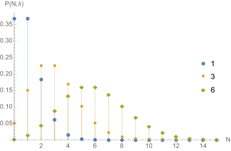
Figure 1: Examples of the Poisson distribution for various values of $\lambda$ as described in the legend.

We can find the mean and standard deviation by direct summation,

$$\langle N\rangle= \sum_{N}^{\infty}NP(N;\lambda)=\lambda e^{-\lambda}\sum_{N}^{\infty}\frac{\lambda^{N}}{N!}=\lambda$$ (2.3.2)

$$\langle N^{2}\rangle= \sum_{N}^{\infty}N^{2}P(N;\lambda)=\lambda e^{-\lambda}\sum_{N}^{\infty}(N+1)\frac{\lambda^{N}}{N!}$$

$$= \lambda e^{-\lambda}(\lambda+1)\sum_{N}^{\infty}\frac{\lambda^{N}}{N!}=\lambda(\lambda+1)$$ (2.3.3)

$$\Rightarrow\sigma^{2}= \ \lambda$$ (2.3.4)

Now let’s take the limit $\lambda\gg 1$. This means the mean, as we just calculated, is also very large, and we allow ourselves to expand around it, parametrising the distribution with the continuous $N(\delta)=\lambda(1+\delta)$, where the region of interest is $|\delta|\ll 1$. Before things get interesting, we need an intermediate result, known as Stirling’s approximation. This is basically an expansion of the $\Gamma$ function defined above in Eq. (2.2.12). Since $n!=\Gamma(n+1)$, we have

$$n!=\int x^{n}e^{-x}\ dx=\int e^{n\log x-x}\ dx$$ (2.3.5)

Now I expand the content of the exponential around the maximum at $x_{0}=n$. This becomes

$$n\log x-x\approx n\log n-n+\frac{1}{2n}(x-n)^{2}$$ (2.3.6)

Inserting this into the integral, we have

$$n!\approx n^{n}e^{-n}\int_{0}^{\infty}e^{(x-n)^{2}/2n}\ dx\approx n^{n}e^{-n}\sqrt{2\pi n}$$ (2.3.7)

where the last integral is done taking the lower limit to minus infinity, as we take $n\gg 1$. Now put all this back into the distribution function,

$$f(\delta;\lambda) \approx\frac{\lambda^{N}}{N^{N}e^{-N}\sqrt{2\pi N}}e^{-\lambda}=\exp\left\{\lambda\delta-(\lambda[1+\delta]+1/2)\log(1+\delta)\right\}\frac{1}{\sqrt{2\pi\lambda}}$$

$$\approx\frac{1}{\sqrt{2\pi\lambda}}\exp\left\{-\frac{\lambda\delta^{2}}{2}\right\}=\frac{1}{\sqrt{2\pi\lambda}}\exp\left\{-\frac{(N-\lambda)^{2}}{2\lambda}\right\}$$ (2.3.8)

where the last approximation expands the content of the exponential to second order in $\delta$ and uses $\lambda\gg 1\gg\delta$. We finally see here the result we might have anticipated, we simply insert the mean and variance of the Poisson distribution in the normal distribution to get the asymptotic expression for the former.

2.3.2   The binomial distribution

This distribution comes about when looking at binary outcomes of a repeated experiment, like a series of coin flips. If the probability of the coin landing heads is $p$, then after $N$ experiments, the probability of obtaining exactly $n$ heads is

$$P(n;N,p)=\begin{pmatrix}N\\ n\end{pmatrix}p^{n}(1-p)^{N-n}$$ (2.3.9)

The first factor on the right hand side is the binomial coefficient

$$\begin{pmatrix}N\\ n\end{pmatrix}=\frac{N!}{n!(N-n)!},$$ (2.3.10)

which takes care of the combinatorics of the different orders of obtaining the $n$ heads. Note that here we have a fixed number of repetitions, where in finding the Poisson distribution, we had a fixed time interval.

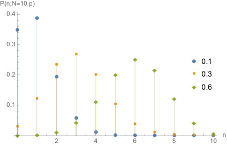
Figure 2: Examples of the binomial distribution for various values of $p$, but fixed $N=10$.

We find again the mean and variance

$$\langle n\rangle =\sum_{n=0}^{N}nP(n;N,p)=Np\sum_{n=1}^{N}\frac{(N-1)!}{(n-1)!(N-n)!}p^{n-1}(1-p)^{N-n}$$

$$=Np\sum_{n=0}^{N-1}P(n;N-1,p)=Np$$ (2.3.11)

$$\langle n^{2}\rangle =Np\sum_{n=0}^{N-1}(n+1)P(n;N-1,p)=Np([N-1]p+1)=(Np)^{2}+Np(1-p)$$

$$\Rightarrow\sigma^{2} =Np(1-p)$$ (2.3.12)

Now consider the double limit $N\rightarrow\infty,p\rightarrow 0$ with the product $Np=\lambda$ fixed. Rewriting the probability distribution using $n\ll N$, we get

$$P(n;\lambda) =\lim_{N\rightarrow\infty}\frac{N!}{n!(N-n)!}\left(\frac{\lambda}{N}\right)^{n}\left(1-\frac{\lambda}{N}\right)^{N-n}$$

$$=\frac{\lambda^{n}}{n!}\lim_{N\rightarrow\infty}\frac{N\cdots(N-n+1)}{N^{n}}\left(1-\frac{\lambda}{N}\right)^{N-n}$$

$$\approx\frac{\lambda^{n}}{n!}e^{-\lambda}$$ (2.3.13)

which is just the Poisson distribution. That means that for a large amount of trials with vanishing probability per trial, the binomial distribution looks just like the Poisson distribution. This makes sense, since we can exactly interpret the infinite trials as being done in continuous time with vanishing probability, such that $Np$ is the rate of success. Taking $\lambda\gg 1$ of course brings us to the gaussian limit again.

2.3.3   The $\chi^{2}$ distribution

We have already seen what this distribution is, along with its moments. Here I quickly show how also this distribution asymptotically looks like a gaussian. I again use Stirling’s approximation to write, in the limit $\nu\rightarrow\infty$, and writing temporarily $x=\nu(1+\delta)$,

$$f(x) =\frac{\nu/2+1}{\sqrt{4\pi\nu}}\left(\frac{e}{\nu/2}\right)^{\nu/2}\left(\frac{\nu}{2}\right)^{\nu/2-1}(1+\delta)^{\nu/2-1}e^{-\nu(1+\delta)/2}$$

$$\approx\frac{1}{\sqrt{2\pi(2\nu)}}e^{-\nu\delta/2+(\nu/2-1)\log(1+\delta)}\approx\frac{1}{\sqrt{2\pi(2\nu)}}\exp\left\{-\frac{\nu\delta^{2}}{4}\right\}$$

$$=\frac{1}{\sqrt{2\pi(2\nu)}}\exp\left\{-\frac{(x-\nu)^{2}}{2(2\nu)}\right\}$$ (2.3.14)

which again is simply a normal distribution with the expected mean and variance.

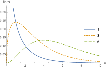
Figure 3: Examples of the $\chi^{2}$ distribution for various values of $\nu$.

2.4   Parameter estimation

An ideal theory will naturally explain all constants involved in it. That means we would very simply be able to compare predictions of this theory with an experiment. However, this is usually not the case. What happens most often is that a theory will contain some unexplained parameter(s), which must be fitted. Supposing the model is true, we can then constrain the parameters of the theory with a particular experiment. This notion of fitting is what the current section explores.

We generally have some experiment, which produces random numbers — due to noise in the experiment or intrinsic variability in the source. How do we compare our model of the experiment to the data produced and in the process fit the parameters of the model? In general these are two different problems, but by the method we are going to use, they can in general be solved simultaneously. The majority of the current section will be about the likelihood and in particular maximising the likelihood, along with finding estimators of the model parameters.

The likelihood is defined as the pdf of the data, $\hat{X}$, given a specific model, which I generically denote $\theta$,

$$\mathcal{L}(\theta)=f(\hat{X}|\theta)$$ (2.4.1)

Note the funny semantics — it is indeed not a probability density of the model, but we still want to link it to some notion of model selection by probability. This has the potential to confuse. One easily avoids this by simply stating what the likelihood is, and never using it as a probability of the model [5]. Note right away that the likelihood is itself in general a random variable, as are the estimators we are going to derive from it.

We now define the maximum likelihood estimators (MLE), $\hat{\theta}$, to be the model parameters, which maximise the likelihood given the obtained data, ie.

$$\frac{\partial\mathcal{L}(\hat{\theta})}{\partial\theta}=0$$ (2.4.2)

These estimators generally have nice properties. The most interesting properties can be found exactly in the context of linear models, which is what I discuss next. In the limit of infinite datasets, these properties extend to non-linear models. I will not discuss this in detail, only illustrate it with an example. For a complete description of the problem and its solution, I refer to textbooks on the subject, eg. [7].

2.4.1   Linear models

Consider a model describing a dataset $\{\hat{x}_{i},\hat{y}_{i}\},\ i=1\dots N$ as

$$y_{i}(x_{i})=\sum_{j=1}^{M}a_{j}A_{j}(x_{i})$$ (2.4.3)

where $M<N$ and the functions $A_{j}$ are fixed and linearly independent, ie. $\sum_{j}a_{j}A_{j}(x_{i})=0\Rightarrow a_{j}=0$. These $A_{j}$ could be monomials, sines and cosines etc. Now assume we measure $x$ with negligible uncertainty and $y$ with some known uncertainty, which we take to be gaussian, ie. $\hat{y}_{i}=y_{i}+\epsilon_{i}$, where $\epsilon_{i}\sim\mathcal{N}(0,1)$. We can now write the likelihood,

$$\mathcal{L}\propto\exp\left\{-\frac{1}{2}\sum_{i}^{N}\left(\hat{y}_{i}-\sum_{j=1}^{M}a_{j}A_{j}(\hat{x}_{i})\right)^{2}\right\}$$ (2.4.4)

The constant of proportionality just normalises the likelihood. Now we want to maximise this likelihood as a function of the $a_{j}$s — the unknown model parameters. Because the exponential is a bit unwieldy, we take the $\log$ and a factor $-2$ out, and instead of maximising $\mathcal{L}$, we minimise $-2\log\mathcal{L}$. The reason for this will hopefully become clear. To find the minimum, we simply solve for the differential to be zero. Doing this, we get a set of $M$ equations for the $M$ $a_{j}$s,

$$\frac{\partial\left(-2\log\mathcal{L}(\hat{a}_{j})\right)}{\partial a_{j}}=0=-2\sum_{i}A_{j}(\hat{x}_{i})\left(\hat{y}_{i}-\sum_{j^{\prime}=1}^{M}\hat{a}_{j^{\prime}}A_{j^{\prime}}(\hat{x}_{i})\right)$$ (2.4.5)

Since we know linear algebra, and this looks an awful lot like it, we drop the indices and see everything as vector-/matrix products. I explicitly define the elements of the matrix $A$ as $A_{ji}=A_{j}(\hat{x}_{i})$, and the sum now looks like

$$0=A(\hat{y}-A^{T}\hat{a})\Rightarrow\hat{a}=(AA^{T})^{-1}A\hat{y}$$ (2.4.6)

The matrix $A$ was defined to have linearly independent rows, which in turn means the inverse of $AA^{T}$ exists. The proof of this is as follows. Define $S=AA^{T}$. Any positive-definite matrix is invertible, so I want to show $S$ is positive definite. We have straight forwardly that for any $X$,

$$X^{T}SX=X^{T}AA^{T}X=|X^{T}A|^{2}\geq 0$$ (2.4.7)

which shows it is positive semi-definite. Now we need to show that if the product is exactly $0$, then so is $X$. Remember the functions $A_{j}$ were assumed to be linearly independent, which means

$$a^{T}A=0\Rightarrow a=0$$ (2.4.8)

This is exactly what we need, since if we write

$$0=X^{T}SX=X^{T}AA^{T}X=|X^{T}A|^{2}\Rightarrow X^{T}A=0\Rightarrow X=0$$ (2.4.9)

This means that $S$ is indeed positive definite and the inverse $(AA^{T})^{-1}$ exists.

Now we are interested in two things: the distribution of $-2\log\mathcal{L}(\hat{a}_{j})$ and of the estimators $\hat{a}_{j}$, under repeated (thought-)experiments. We first look at the likelihood.

$$-2\log\mathcal{L}(\hat{a}) =|\hat{y}-A^{T}\hat{a}|^{2}=|\hat{y}-A^{T}(AA^{T})^{-1}A\hat{y}|^{2}$$

$$=\left|\left(\mathbb{1}_{N}-A^{T}(AA^{T})^{-1}A\right)\hat{y}\right|^{2}$$ (2.4.10)

Here $P=A^{T}(AA^{T})^{-1}A$ is a projection in the sense $P^{2}X=PX$ for any $X\in\mathbb{R}^{N}$ to an $M$ dimensional subspace. By an orthogonal transformation, we can rotate the $\hat{y}$ to $\tilde{y}=\mathcal{O}\hat{y}$ such that the projection $P\tilde{y}$ has its elements only in the first $M$ entries, ie. $P(\tilde{y}_{1},\dots,\tilde{y}_{N})^{T}=(\tilde{y}_{1},\dots,\tilde{y}_{M},0,\dots,0)^{T}$. Note that since the transformation is orthogonal, we also have $\tilde{y}_{i}\sim\mathcal{N}(0,1)$. Taking now $\bar{y}=(\mathbb{1}_{N}-P)\tilde{y}=(0,\dots,0,\tilde{y}_{M+1},\dots,\tilde{y}_{N})^{T}$, the likelihood takes the following form

$$-2\log\mathcal{L}(\hat{a})=\bar{y}^{T}\bar{y}=\sum_{i=M+1}^{N}\tilde{y}_{i}^{2}\sim\chi^{2}_{\nu=N-M}$$ (2.4.11)

This result is the origin of two notions, which are often abused in practice. The first is, we simply call $-2\log\mathcal{L}$ the chi squared, $\chi^{2}$. This may result in a bit of confusion since now one has a random variable called $\chi^{2}$, which is $\chi^{2}$-distributed, ie. its pdf is the $\chi^{2}$ distribution. The other is the idea of a reduced number of degrees of freedom, $\nu=N-M$, ie. the number of data points minus the number of fit parameters. These ideas are widely used even when the model is not linear.

Now we turn to the distribution of the estimators $\hat{a}$. We have already seen the result, which is

$$\hat{a} =(AA^{T})^{-1}A\hat{y}\Rightarrow\hat{a}\sim\mathcal{N}(a,(AA^{T})^{-1})=\mathcal{N}(a,\mathcal{I}^{-1}),$$ (2.4.12)

where the normal distribution is to be understood in the multivariate sense. We see here a specific example of a more general result. The MLE is normally distributed around the true value — it is unbiased — with covariance matrix described by

$$\Sigma_{\hat{a}} \geq\mathcal{I}(\hat{a})^{-1},\hskip 28.45274pt\text{where}$$ (2.4.13)

$$\mathcal{I}(\hat{a})_{ij} =\left\langle\frac{\partial^{2}(-\log\mathcal{L}(\hat{a}))}{\partial a_{i}\partial a_{j}}\right\rangle$$ (2.4.14)

where the average is taken over repeated experiments. $\mathcal{I}=AA^{T}$ is called the Fisher Information. In this case, the double derivative is a constant, so the average is trivial. This bound on the covariance matrix is called the Cramér-Rao bound, and is the minimal covariance for unbiased estimators. An unbiased estimator with this minimal variance is called efficient. We see that the MLE for linear models are all exactly unbiased, normally distributed, efficient estimators for all $N$.

The linear models are nice because, as we have just seen, practically everything can be done analytically. This gives us a nice starting point for the next discussion. For a general, non-linear model, the results in the example are no longer valid. Let us explore finite sample sizes with a very simple example.

2.4.2   A non-linear model

Consider the data set $\{\hat{x}_{i}\},\ i=1\dots N$, drawn from a normal distribution with unknown mean and variance, but with no measurement uncertainty, $x_{i}\sim\mathcal{N}(\mu,\sigma)$. The likelihood for this experiment is

$$\mathcal{L}=(2\pi\sigma^{2})^{-N/2}\exp\left\{-\frac{1}{2}\sum_{i}^{N}\left(\frac{\hat{x}_{i}-\mu}{\sigma}\right)^{2}\right\}$$ (2.4.15)

and we are trying to determine $\mu$ and $\sigma^{2}$. Note how we cannot neglect the normalisation this time, since we are now fitting $\sigma$. The maximum point $(\hat{\mu},\hat{\sigma}^{2})$ is

$$\hat{\mu} =N^{-1}\sum_{i}\hat{x}_{i}$$ (2.4.16)

$$\hat{\sigma}^{2} =\sum_{i}(\hat{x}_{i}-\hat{\mu})^{2}$$ (2.4.17)

Now consider the distribution of these estimators. The fact that we don’t know $\sigma$ complicates things, since this is what set the scale for us before — we could measure deviations in terms of a fixed number. Now this scale is a random variable. For instance, we immediately see that $\hat{\mu}\sim\mathcal{N}(\mu,\sigma/\sqrt{N})$, but here we’ve used the unknown $\sigma$ to define the variance.

We turn therefore first to the distribution of the variance $\sigma^{2}$. I first write out the $\hat{\mu}$ and rewrite the sum, giving

$$\hat{\sigma}^{2}=N^{-2}\sum_{ij}(\hat{x}_{i}-\hat{x}_{j})^{2}$$ (2.4.18)

We now need a small trick to evaluate this sum. What we really want — anticipating the answer — is something like a sum of squares $\sum x_{i}x_{j}$, not of squares of differences, as we have. So we recast it to

$$\hat{\sigma}^{2}=N^{-1}\sum_{ij}x_{i}C_{ij}x_{j}$$ (2.4.19)

and find the matrix $C$ we need here is

$$C=\begin{pmatrix}1-N^{-1}&-N^{-1}&\cdots\\ -N^{-1}&1-N^{-1}&\\ \vdots&&\ddots\end{pmatrix},\ |C|=0$$ (2.4.20)

We now pseudo Cholesky factorise $C$, ie. we find an upper triangular matrix $U$, which satisfies $U^{T}U=C$. This matrix is

$$U_{ij}=\left\{\begin{matrix}\sqrt{(N-i)/(N+1-i)}&i=j\\ -1/\sqrt{(N-i)(N+1-i)}&i<j\\ 0&i>j\end{matrix}\right.$$ (2.4.21)

We now use $U$ to find the rank of $C$, which determines the pdf of the sum. Taking the reverse product, we see that

$$UU^{\text{T}}=\begin{pmatrix}1&0&\cdots&&\\ 0&1&&\\ \vdots&&\ddots&\\ &&&1&0\\ &&&0&0\end{pmatrix},$$ (2.4.22)

which immediately tells us the rank of $C$ is $N-1$. This means $U$ is almost an orthogonal transformation — we just lose one degree of freedom. Thus we will define new variables $y_{j}=\sum_{i}U_{ji}x_{i},\ j=1\dots N-1$, which are also drawn from independent normal distributions. The variance is now given as

$$N\hat{\sigma}^{2} =\sum_{ij}x_{i}C_{ij}x_{j}=\sum_{ijk}x_{i}U_{ki}U_{kj}x_{j}$$

$$=\sum_{i}(Ux)_{i}^{2}=\sum_{i}^{N-1}y_{i}^{2}\sim\sigma^{2}\chi^{2}_{\nu=N-1}$$ (2.4.23)

This shows that for finite $N$, the estimator is a bit off, as

$$\langle\hat{\sigma}^{2}\rangle=\sigma^{2}\frac{N-1}{N}$$ (2.4.24)

This comes about because we fit the mean while calculating it. The missing degree of freedom is of course the mean $\hat{\mu}$ which we now consider. Had we known $\sigma$, we would immediately write $\sqrt{N}(\hat{\mu}-\mu)/\sigma\sim\mathcal{N}(0,1)$. Exchanging $\sigma$ for $\hat{\sigma}$, the distribution changes a bit. We may write

$$\sqrt{N}(\hat{\mu}-\mu)/\hat{\sigma}=\frac{n}{c}$$ (2.4.25)

where $n$ is normally distributed $n\sim\mathcal{N}(0,1)$ and $c$ follows a $\chi$ distribution, $c\sim\chi_{\nu=N-1}$. Note how this combination exactly cancels the dependence of $\sigma$. This particular combination of random variables follows a distribution known as Student’s t-distribution with $\nu=N-1$ degrees of freedom. Its pdf is

$$f(x;\nu)=\frac{\Gamma(\frac{\nu+1}{2})}{\sqrt{\nu\pi}\Gamma(\frac{\nu}{2})}\left(1+\frac{x^{2}}{\nu}\right)^{-\frac{\nu+1}{2}}$$ (2.4.26)

We are now in a position to understand the $N\rightarrow\infty$ limit of the MLE. We see that for finite $N$, neither of the two estimators follow a normal distribution, and $\hat{\sigma}^{2}$ is even biased. In the asymptotic limit though, both distributions are normal, and we have

$$\sqrt{N}(\hat{\mu}-\mu)/\hat{\sigma}\sim\mathcal{N}(0,1) \Rightarrow\hat{\mu}\sim\mathcal{N}(\mu,\hat{\sigma}/\sqrt{N})$$ (2.4.27)

$$N\hat{\sigma}^{2}/\sigma^{2}\sim\mathcal{N}(N,\sqrt{2N}) \Rightarrow\hat{\sigma}^{2}\sim\mathcal{N}(\sigma^{2},\sqrt{\frac{2}{N}}\sigma^{2})$$ (2.4.28)

It is only in the asymptotic limit the estimators follow an unbiased normal distribution, with variance given by Eq. (2.4.13). As I showed earlier, many distributions tend to a normal distribution for large $N$. This is what is happening here too. In this limit, the likelihood tends to a normal distribution, for which the results from the previous section hold.

2.4.3   Cramér-Rao lower bound

Now let us see how the Cramér-Rao bound appears. I will follow the proof from [7]. Assume we have a set of unbiased estimators $\{\hat{g}_{i}\},i=1\dots r$, of the quantities $\{g_{i}\}$, ie. $\langle\hat{g}_{i}\rangle=g_{i}$. The likelihood function generally depends on some parameters, say $\theta_{j},j=1\dots k$. We now construct another set of variables, $\{\frac{\partial\log\mathcal{L}}{\partial\theta_{j}}\}$, and build the $r+k$-vector $\{\hat{g}_{1}\dots\hat{g}_{r},\frac{\partial\log\mathcal{L}}{\partial\theta_{1}}\dots\frac{\partial\log\mathcal{L}}{\partial\theta_{k}}\}$. The covariance matrix of this vector is

$$\begin{pmatrix}\Sigma_{\hat{g}}&\Delta\\ \Delta^{T}&\mathcal{I}\end{pmatrix}$$ (2.4.29)

Where $\Sigma_{\hat{g}}$ is the covariance of the estimators $\hat{g}$, $\mathcal{I}$ is the Fisher Information and

$$\Delta_{ij}=\int\hat{g}_{i}\frac{\partial\log\mathcal{L}}{\partial\theta_{j}}\mathcal{L}\ dx=\int\hat{g}_{i}\frac{\partial\mathcal{L}}{\partial\theta_{j}}\ dx=\frac{\partial g_{i}}{\partial\theta_{j}}$$ (2.4.30)

By construction, this covariance matrix is positive definite. Furthermore, we have that

$$\left|\begin{matrix}\mathbb{1}&-\Delta\mathcal{I}^{-1}\\ 0&\mathcal{I}^{-1}\end{matrix}\right|=|\mathcal{I}|^{-1}\geq 0$$ (2.4.31)

since the Fisher Information is positive definite. This is seen easily since we can rewrite it as

$$\mathcal{I}_{ij} =\left\langle\frac{\partial^{2}(-\log\mathcal{L})}{\partial\theta_{i}\partial\theta_{j}}\right\rangle=\left\langle\frac{\partial\log\mathcal{L}}{\partial\theta_{i}}\frac{\partial\log\mathcal{L}}{\partial\theta_{j}}\right\rangle$$

$$\Rightarrow q^{T}\mathcal{I}q =\left\langle\left(\sum_{i}\frac{\partial\log\mathcal{L}}{\partial\theta_{i}}q_{i}\right)^{2}\right\rangle\geq 0$$ (2.4.32)

By multiplying the two matrices, we see that

$$\left|\begin{matrix}\mathbb{1}&-\Delta\mathcal{I}^{-1}\\ 0&\mathcal{I}^{-1}\end{matrix}\right|\times\left|\begin{matrix}\Sigma_{\hat{g}}&\Delta\\ \Delta^{T}&\mathcal{I}\end{matrix}\right|=\left|\begin{matrix}\Sigma_{\hat{g}}-\Delta\mathcal{I}\Delta^{T}&0\\ \mathcal{I}^{-1}\Delta^{T}&\mathbb{1}\end{matrix}\right|=\left|\Sigma_{\hat{g}}-\Delta\mathcal{I}^{-1}\Delta^{T}\right|\geq 0,$$ (2.4.33)

which holds for any subset of the estimators $\hat{g}$. From this it follows that all eigenvalues of $\Sigma_{\hat{g}}-\Delta\mathcal{I}^{-1}\Delta^{T}$ are positive or zero, or equivalently that the matrix is positive semi-definite. Looking at unbiased estimators of the $\theta$s, we see that $\Delta$ reduces to an identity matrix and the bound dictates the matrix $\Sigma_{\hat{\theta}}-\mathcal{I}^{-1}$ is positive semi-definite. This is exactly what is meant in Eq. (2.4.13).

Note however, that in deriving this bound, we rely on the estimator being unbiased. It is easy to think of estimators with lower variance, say $\hat{g}=1$. This has obviously zero variance, but is not a particularly good estimator of anything. It is also worth noting that this bound does not require that the estimator follows a normal distribution. It sets a bound on the variance of any unbiased estimator. However, it is only a lower bound, and by no means a guarantee — only in special cases, like the MLE of a linear model, does an estimator saturate the bound exactly.

2.4.4   Confidence regions

Having found the distributions of the estimators of the parameters of a theory, I now want to define the notion of confidence regions. Loosely speaking, these are regions in which we are confident the true value of the parameter lies. This confidence is usually defined in terms of a coverage probability, $p_{c}$. That is, if we define our confidence regions in the same way in repeat experiments, then for every repetition we have the probability $p_{c}$ that $\theta$ is inside our confidence region. The usual objection here is that once the experiment is done, we can no longer speak of a probability that the true $\theta$ is inside or outside the confidence region — it either is or is not! The probability as such is defined prior to the experiment. This distinction shall not worry us too much.

To begin the discussion on confidence regions, we have to understand the concept of a p-value, which is closely related to the coverage probability. This is very simple. The p-value of some event is the probability of seeing something more extreme or as extreme as what is observed. In different scenarios this may be computed in a variety of ways, depending on the difficulty of the problem at hand. In some cases, p-values can be computed analytically, while for others one resorts to Monte Carlo (MC), ie. random simulations. As such, the p-value is entirely dependent on the model being tested, and is only telling us how unlikely something is, given a specific model. Let us see how this works in an example.

A fair coin?   Consider tossing the same coin $N$ times. We now ask ourselves the question ”is the coin fair?”, and we can address the answer with a p-value. Say the coin lands heads up $M$ times, where without loss of generality, $M\geq N/2$. To calculate the p-value, we now simply add up the probabilities of getting $M$ or more heads when tossing a fair coin,

$$p =\sum_{m=M}^{N}\begin{pmatrix}N\\ m\end{pmatrix}0.5^{m}0.5^{N-m}=\sum_{m=M}^{N}\begin{pmatrix}N\\ m\end{pmatrix}0.5^{N}$$

$$=0.5^{N}\begin{pmatrix}N\\ M\end{pmatrix}\phantom{}_{2}F_{1}(1,M-N,1+M;-1),$$ (2.4.34)

where $\phantom{}{}_{2}F_{1}$ is the hypergeometric function, whose form is not particularly enlightening. To make things more clear, let’s take a specific example. In Fig. 4 I take various values for $N$ and plot the p-value one would obtain as a function of $M$. The line across denotes the custom $95\%$ confidence level, ie. everything under the line is excluded at more than $95\%$ confidence. It is evident that the as $N$ goes up, we need a smaller and smaller relative deviation from $M=N/2$ before we can exclude that the coin is fair. Figure 4: p-value, given by Eq. (2.4.34), of different outcomes $M$ from tossing a coin $N$ times for different values of $N$ as labeled in the legend. This tests the hypothesis that the coin is fair.

Originally we wanted to constrain our parameters. With the p-value at hand, we just need Wilks’ theorem, which tells us the distribution of a likelihood ratio in terms of a $\chi^{2}$ distribution. This was first shown in [8]. First I go through the proof of the theorem, and following that, we will see how this constrains our parameters through confidence regions. I will here just look at a linear model, and I simply argue that the results we find extend to non-linear models in the asymptotic limit — and that we abuse this fact and use Wilks’ theorem always.

Consider the type of model from Sec. 2.4.1. Take a space for the possible coefficients, $\Omega$, and a subset $\bot\in\Omega$ of dimensions $N$ and $M$ respectively, so $0\leq M<N$. Now call the true parameters $a_{\Omega}\equiv\{a_{\bot},a_{\omega}\}$, where $a_{\omega}\in\omega,a_{\bot}\in\bot=\omega^{\bot}$. We can see $\bot$ as the remaining part of $\Omega$, when we fix $a_{\omega}$. Now we have both the MLE $\hat{a}_{\Omega}=\{\hat{a}_{\bot},\hat{a}_{\omega}\}\in\Omega$ and a restricted MLE $\hat{\hat{a}}_{\bot}\in\bot$, which satisfy

$$\frac{\partial\log\mathcal{L}(\hat{a}_{\Omega})}{\partial a_{i}} =0,\hskip 28.45274pti=1\dots N$$ (2.4.35)

$$\frac{\partial\log\mathcal{L}(\hat{\hat{a}}_{\bot},a_{\omega})}{\partial a_{i}} =0,\hskip 28.45274pti=1\dots M$$ (2.4.36)

The quantity $\mathcal{L}_{p}(a_{\omega})=\mathcal{L}(\hat{\hat{a}}_{\bot},a_{\omega})$ is called the profile likelihood. $\hat{\hat{a}}_{\bot}$ is given by

$$\hat{\hat{a}}_{\bot}=\hat{a}_{\bot}-\mathcal{I}_{\bot}^{-1}\tilde{\mathcal{I}}(a_{\omega}-\hat{a}_{\omega})$$ (2.4.37)

where I have partitioned the Fisher Information as

$$\mathcal{I}_{\Omega}=\begin{pmatrix}\mathcal{I}_{\bot}&\tilde{\mathcal{I}}\\ \tilde{\mathcal{I}}^{T}&\mathcal{I}_{\omega}\end{pmatrix}$$ (2.4.38)

Now I define the likelihood ratio

$$\lambda=\frac{\mathcal{L}(\hat{\hat{a}}_{\bot},a_{\omega})}{\mathcal{L}(\hat{a}_{\Omega})}$$ (2.4.39)

and seek the distribution of this under the hypothesis that $a_{\omega}$ are indeed the true parameters. Take $-2\log$ of this and insert factors of the true likelihood $\mathcal{L}(a_{\Omega})$,

$$-2\log\lambda=-2\log\frac{\mathcal{L}(\hat{\hat{a}}_{\bot},a_{\omega})}{\mathcal{L}(a_{\Omega})}+2\log\frac{\mathcal{L}(\hat{a}_{\Omega})}{\mathcal{L}(a_{\Omega})}$$ (2.4.40)

Each of the terms on the right hand side can be reduced to the forms

$$-2\log\frac{\mathcal{L}(\hat{\hat{a}}_{\bot},a_{\omega})}{\mathcal{L}(a_{\Omega})} =-(\hat{\hat{a}}_{\bot}-a_{\bot})^{T}\mathcal{I}_{\bot}(\hat{\hat{a}}_{\bot}-a_{\bot})$$ (2.4.41)

$$2\log\frac{\mathcal{L}(\hat{a}_{\Omega})}{\mathcal{L}(a_{\Omega})} =(\hat{a}_{\Omega}-a_{\Omega})^{T}\mathcal{I}_{\Omega}(\hat{a}_{\Omega}-a_{\Omega})$$ (2.4.42)

This is seen by simply inserting the MLE, Eq. (2.4.6) into Eq. (2.4.4) and collecting terms. Now write the derivative of the log-likelihood at the true parameters $a_{\Omega}$, split into the $\bot$ and $\omega$ parts as

$$\begin{pmatrix}\eta\\ \xi\end{pmatrix}_{i}=\frac{\partial\log\mathcal{L}(a_{\Omega})}{\partial a_{i}}$$ (2.4.43)

This gives two expressions for $\eta$ and one for $\xi$,

$$\begin{pmatrix}\eta\\ \xi\end{pmatrix} =\mathcal{I}_{\Omega}(\hat{a}_{\Omega}-a_{\Omega})$$ (2.4.44)

$$\eta =\mathcal{I}_{\bot}(\hat{\hat{a}}_{\bot}-a_{\bot})$$ (2.4.45)

Remember, since the estimators follow the distribution in Eq. (2.4.12), these variables follow a normal distribution $(\eta,\xi)_{i}\sim\mathcal{N}(0,\mathcal{I}_{\Omega})$. Inserting this into Eq. (2.4.40), we have

$$-2\log\lambda=\begin{pmatrix}\eta\\ \xi\end{pmatrix}^{T}\mathcal{I}_{\Omega}^{-1}\begin{pmatrix}\eta\\ \xi\end{pmatrix}-\eta\mathcal{I}_{\bot}^{-1}\eta$$ (2.4.46)

Using the following block inversion identity

$$\mathcal{I}_{\Omega}^{-1}=\begin{pmatrix}\mathcal{I}_{\bot}^{-1}+\mathcal{I}_{\bot}^{-1}\tilde{\mathcal{I}}(\mathcal{I}_{\omega}-\tilde{\mathcal{I}}^{T}\mathcal{I}_{\bot}^{-1}\tilde{\mathcal{I}})^{-1}\tilde{\mathcal{I}}^{T}\mathcal{I}_{\bot}^{-1}&-\mathcal{I}_{\bot}^{-1}\tilde{\mathcal{I}}(\mathcal{I}_{\omega}-\tilde{\mathcal{I}}^{T}\mathcal{I}_{\bot}^{-1}\tilde{\mathcal{I}})^{-1}\\ -(\mathcal{I}_{\omega}-\tilde{\mathcal{I}}^{T}\mathcal{I}_{\bot}^{-1}\tilde{\mathcal{I}})^{-1}\tilde{\mathcal{I}}^{T}\mathcal{I}_{\bot}^{-1}&(\mathcal{I}_{\omega}-\tilde{\mathcal{I}}^{T}\mathcal{I}_{\bot}^{-1}\tilde{\mathcal{I}})^{-1}\end{pmatrix}$$ (2.4.47)

we can write the first product in Eq. (2.4.46) as

$$\eta^{T}\mathcal{I}_{\bot}^{-1}\eta+(\tilde{\mathcal{I}}^{T}\mathcal{I}_{\bot}^{-1}\eta-\xi)^{T}(\mathcal{I}_{\omega}-\tilde{\mathcal{I}}^{T}\mathcal{I}_{\bot}^{-1}\tilde{\mathcal{I}})^{-1}(\tilde{\mathcal{I}}^{T}\mathcal{I}_{\bot}^{-1}\eta-\xi)$$ (2.4.48)

The first term here is subtracted in the likelihood ratio, and we have

$$-2\log\lambda=(\tilde{\mathcal{I}}^{T}\mathcal{I}_{\bot}^{-1}\eta-\xi)^{T}(\mathcal{I}_{\omega}-\tilde{\mathcal{I}}^{T}\mathcal{I}_{\bot}^{-1}\tilde{\mathcal{I}})^{-1}(\tilde{\mathcal{I}}^{T}\mathcal{I}_{\bot}^{-1}\eta-\xi)$$ (2.4.49)

This combination of variables, $\tilde{\mathcal{I}}^{T}\mathcal{I}_{\bot}^{-1}\eta-\xi$ again follows a normal distribution, for which the covariance is easily seen to be

$$\left\langle(\tilde{\mathcal{I}}^{T}\mathcal{I}_{\bot}^{-1}\eta-\xi)(\tilde{\mathcal{I}}^{T}\mathcal{I}_{\bot}^{-1}\eta-\xi)^{T}\right\rangle= \left\langle\xi\xi^{T}-2\tilde{\mathcal{I}}^{T}\mathcal{I}_{\bot}^{-1}\eta\xi^{T}+\tilde{\mathcal{I}}^{T}\mathcal{I}_{\bot}^{-1}\eta\eta^{T}\mathcal{I}_{\bot}^{-1}\tilde{\mathcal{I}}\right\rangle$$

$$= (\mathcal{I}_{\omega}-\tilde{\mathcal{I}}^{T}\mathcal{I}_{\bot}^{-1}\tilde{\mathcal{I}})$$ (2.4.50)

Meaning the likelihood ratio is simply the sum the squares of $N-M$ — the number of fixed dimensions — independent gaussian random variables

$$-2\log\lambda\sim\chi^{2}_{\nu=N-M}$$ (2.4.51)

To test the hypothesis that $a_{\omega}$ are the true parameters, we now simply find the p-value of getting the particular $-2\log\lambda$ value for that $a_{\omega}$. This p-value is given by

$$\text{p-value}=\int_{-2\log\lambda}^{\infty}\chi^{2}_{\nu=N-M}(x)\ dx$$ (2.4.52)

To illustrate this, let’s look at an example.

Constraining a one-parameter linear model   Consider drawing from a gaussian distribution with known variance, say $\sigma=1$, but unknown mean $\mu$. The likelihood is of the form Eq. (2.4.4), specifically

$$\mathcal{L}(\mu)\propto\exp\left\{-\frac{1}{2}\sum_{i}(\hat{y}_{i}-\mu)^{2}\right\}$$ (2.4.53)

and we want to say something about $\mu$ given some experimental result. For a particular outcome of the experiment, say $N$ datapoints, we use Wilks’ theorem in the following way. We take as $\Omega$ the full range of the $\mu$, for which we find the MLE as

$$\hat{\mu}=N^{-1}\sum_{i}\hat{y}_{i}$$ (2.4.54)

and for every possible value of $\mu$, we take $\omega$ as just that $\mu$. Since there are no parameters left, the restricted MLE in $\bot$ is trivial. The p-value is calculated according to Eq. (2.4.52),

$$\text{p-value}(\mu) =\int_{-2\log\lambda(\mu)}^{\infty}\chi^{2}_{\nu=1}(x)\ dx$$ where (2.4.55)

$$-2\log\lambda(\mu) =-2\log[\mathcal{L}(\mu)/\mathcal{L}(\hat{\mu})]=N(\mu-\hat{\mu})^{2}$$ (2.4.56)

I now choose to look at the values $\mu_{n}=\hat{\mu}(1\pm n/\sqrt{N})$ for various $n$. This gives us the integral, for $n=\{1,2,3\}$,

$$\text{p-value}(\mu_{n})=\int_{n^{2}}^{\infty}\chi^{2}_{\nu=1}(x)\ dx=\{0.32,0.046,0.0027\}$$ (2.4.57)

Or in words, we can exclude these values with confidence $\{0.68,0.954,0.9973\}$. Say we want to be at least $68\%$ confident, then our confidence region is $\hat{\mu}\pm\frac{\hat{\mu}}{\sqrt{N}}\equiv[\hat{\mu}(1-\frac{1}{\sqrt{N}}),\hat{\mu}(1+\frac{1}{\sqrt{N}})]$, ie. no values inside this interval can be excluded with confidence greater than 68%.

Because of the gaussian nature of the likelihood ratio, this limit is usually called the $1$-$\sigma$ confidence interval, as it is exactly one standard deviation away from the mean, and the standard deviation is usually denoted $\sigma$. We can in the same fashion construct the $n$-$\sigma$ interval for the other $n$s.

The previous example simply shows the general use of Wilks’ theorem. Another subtle thing we can do is to eliminate parameters, which are not of immediate interest. Such parameters are usually called nuisance parameters. To see how this works, we just have to have one more parameter. The following example is trivially extended to $N$ parameters of which $M<N$ are nuisance parameters. Unfortunately the 2 dimensional nature of paper only allows for easy visualisation of 2 dimensions.

Eliminating nuisance parameters   Consider a two-parameter linear model with the general likelihood, in vector notation,

$$\mathcal{L}(a)\propto\exp\left\{-\frac{1}{2}(\hat{y}-A^{T}a)^{2}\right\}$$ (2.4.58)

with $a=\{a_{\bot},a_{\omega}\}$ and $y\in\mathbb{R}^{N}$. As stated before, the MLE is given by Eq. (2.4.6), $\hat{a}=(AA^{T})^{-1}A\hat{y}$. First, let’s do the same thing we did before, and let $\Omega$ be the entire space of $a$, while $\omega$ fixes both parameters, ie. $\Omega=\omega$. That makes the likelihood ratio

$$-2\log\lambda(a)=(a-\hat{a})^{T}\mathcal{I}(a-\hat{a})$$ (2.4.59)

a random $\chi^{2}_{\nu=2}$ variable for which we again calculate p-values according to Eq. (2.4.52).

Now one of the parameters $a_{\bot}$ is a nuisance parameter. This means that we only fix $a_{\omega}$, and find the constrained maximum over $a_{\bot}$. So we look at the quantity

$$-2\log\tilde{\lambda}(a_{\omega})=-2\log\frac{\mathcal{L}(\hat{\hat{a}}_{\bot},a_{\omega})}{\mathcal{L}(\hat{a})},$$ (2.4.60)

Now, by Wilks’ theorem, this quantity is a random $\chi^{2}_{\nu=1}$ variable. The last two points are illustrated in Fig. 5. For the sake of illustration, the parameters are taken to be very correlated. Figure 5: Illustration of confidence regions for two parameters with $\mathcal{I}_{\bot}=\mathcal{I}_{\omega}=1,\tilde{\mathcal{I}}=1/\sqrt{2}$. The dashed contour shows the $68\%$ confidence region of both parameters, while the dotted lines are the boundaries of the $68\%$ $a_{\omega}$ confidence interval, taking $a_{\bot}$ to be a nuisance parameter. As shown, these dotted lines mark the extreme $a_{\omega}$ for which any $a_{\bot}$ gives $-2\log\lambda\leq 1$. The number $2.3$ is the solution $y$ to the equation $\int_{y}^{\infty}\chi^{2}_{\nu=2}(x)\ dx=1-0.68$. For higher dimensions, one could also give the boundaries of the joint contour in lower dimensions — here the boundary would be at $\pm\sqrt{2.3}$ instead of $1$. It is important though, to remember the difference in meaning. The bigger one also contains information on the other parameter, while the small one take all but $a_{\omega}$ as nuisance parameters.

We see that the question which Wilks’ theorem helps us answer is if we can confidently exclude some parameters $a_{\omega}$ for all values of the remaining parameters $a_{\bot}$. Even if there is just a single set of parameters $\{a_{\bot},a_{\omega}\}$ such that the p-value is big enough, ie. $-2\log\lambda$ is small enough, then $a_{\omega}$ cannot be excluded. From Fig. 5 we see exactly how for $a_{\omega}=\sqrt{2}$, we only have $-\log\tilde{\lambda}\leq 1$ when $a_{\bot}=1$. This still means $a_{\omega}=\sqrt{2}$ cannot be excluded at $1\sigma$. Said differently, for every $a_{\omega}$ we test the hypothesis that this is the true value, regardless of what the $a_{\bot}$ parameter is.

2.4.5   Marginalisation

In the previous derivation, I strictly refer to maximisation of likelihoods. Even so, one will often encounter the term marginalised likelihood. The use of this should be kept to a minimum outside Bayesian reasoning, which is described briefly in Sec. 2.6. Marginalising the likelihood in simply integration instead of maximisation. That is, instead of using $\mathcal{L}_{p}$, we define the marginal likelihood

$$\mathcal{L}_{m}(\theta)=\int\mathcal{L}(\theta,\phi)\ d\phi$$ (2.4.61)

A trivial exercise is to show that the confidence regions determined from this quantity is in general not the same as one would get with the profile likelihood. The objection is now that, obviously, the marginal likelihood is not reparametrisation invariant, ie. for some other parametrisation of the nuisance parameters $\Phi=f(\phi)$,

$$\int\mathcal{L}(\theta,\phi)\ d\phi\neq\int\mathcal{L}(\theta,\Phi)\ d\Phi$$ (2.4.62)

The two integrands differ by a jacobian $J=d\phi/d\Phi$. This means that when you pick your parametrisation for the likelihood, you assume in some sense that this is a good parametrisation. This again reflects the issue that the likelihood is not a pdf of the model — that is why the meaning of this integral is not immediate.

Now it is an equally easy exercise to convince oneself that the maximisation procedure is completely free of this caveat. The maximum likelihood for some $\theta$ cannot depend on the chosen parametrisation of $\phi$, so obviously $\max_{\phi}\mathcal{L}(\theta,\phi)=\max_{\Phi}\mathcal{L}(\theta,\Phi)$.

2.5   Monte Carlo methods

The previous sections have mostly described linear models, and in one case a very simple non-linear model, whose answer can be found analytically. This, unfortunately, is not always the case. For some random variables, it can be impossible to find explicit expressions for their distributions. When this happens, as is often the case, one way around it is to simply simulate the distribution. This approach is broadly called Monte Carlo (MC) methods, and underlies many results of modern physics. The approach can also be applied to numerical evaluation of integrals. To see this, let’s go through the classic example, where we find $\pi\approx 3.14$ by MC integration.

Estimating $\pi$   We know the ratio of areas of a unit circle to a square with side length $2$ to be $\pi/4$. Now as an exercise we want to find the value of this numerically. We look at a single quadrant, $x\in[0,1],\ y\in[0,1]$, where the ratio of areas is the same. We now draw $N$ points inside this region and for every point check if it is inside or outside the circle. So for every point, check if $\sqrt{x^{2}+y^{2}}\leq 1$. Finally, we count the number inside the circle, call it $M$, and divide by $N$. The ratio $M/N$ estimates $\pi/4$ (since the region from which we draw has unit area).

Now, since we are doing this as MC, the estimate we get has an associated error, which we must also estimate. Namely, for every point we draw, it has the probability $\pi/4$ to be inside the circle. That means $M$ will be binomial distributed with $p=\pi/4$ with $N$ draws. From our previous calculations (2.3.11)-(2.3.12), we get immediately

$$\langle M\rangle=N\cdot\pi/4$$ (2.5.1)

$$\sigma_{M}^{2}=N\cdot\pi/4(1-\pi/4)$$ (2.5.2)

or, if we look at the quantity $M/N$, and approximate the binomial with $N$ very large as a gaussian,

$$M/N\sim\mathcal{N}(\pi/4,\sqrt{\pi/4(1-\pi/4)/N}).$$ (2.5.3)

We see here a very general (approximate) result: the error on the estimate falls off as $\sqrt{N}^{-1}$. So, not surprisingly, the larger we take $N$, the better the approximation we get. This is illustrated in Figs. 6 and 7. This technique is in its most naive form extended trivially to any integral in any number of dimensions. Of course, as the parameter space becomes larger, computing time increases, but the basic picture remains. Figure 6: Example of MC integration. Each point is drawn at random. In this case, $N=10^{3},\ M=781$. This means the $1\sigma$ confidence interval for the integral is approximately $(\pi/4)_{\text{MC}}=0.781\pm 0.013$, compared to the true value, $\pi/4=0.7853$, we see that this is indeed a reasonable estimate. Figure 7: Errors from the computation of $\pi$ by MC integration. We see that all the errors are of expected magnitude (notice that it is plotted on log-log axes). For every $N$, I perform $10$ MC simulations, simply to show the intrinsic variability in the estimate.

So we can do integrals numerically. This is comforting! As mentioned earlier, we also might want to find distributions for which we cannot find an analytic expression. This is heavily used when finding p-values for some non-trivial quantity. What one does is to simulate an experiment a number of times, say $N$, and for every simulation find the desired quantity. The distribution of these simulated quantities then answers the same question as would the analytic expression, given this model, how (un)likely is the observed outcome, simply by numerical comparison between the MC results and the real experiment. I will now extend the previous non-linear model of Sec. 2.4.2 very slightly, and we shall see that we immediately lose the analytic expression for the estimators. We will then use MC to regain control.

Unequal errors on measurements   Take again the estimation of a normal distribution with $(\mu,\sigma^{2})=(0,1)$, but this time add distinct measurement errors, $\sigma_{i}$, on all $\hat{x}_{i}$s. This means the likelihood is

$$\mathcal{L}=\prod_{i}^{N}(2\pi[\sigma^{2}+\sigma_{i}^{2}])^{-1/2}\exp\left\{-\frac{1}{2}\frac{(\hat{x}_{i}-\mu)^{2}}{\sigma^{2}+\sigma_{i}^{2}}\right\}$$ (2.5.4)

Looking for the MLE $(\hat{\mu},\hat{\sigma}^{2})$ of this model, we get

$$\hat{\mu}= \frac{\sum\hat{x}_{i}/(\sigma^{2}+\sigma_{i}^{2})}{\sum 1/(\hat{\sigma}^{2}+\sigma_{i}^{2})}$$ (2.5.5)

$$\sum 1/(\hat{\sigma}^{2}+\sigma_{i}^{2})= \sum\frac{(\hat{x}_{i}-\hat{\mu})^{2}}{(\hat{\sigma}^{2}+\sigma_{i}^{2})^{2}}$$ (2.5.6)

The appearance of $\sigma_{i}$ in these sums prohibits the nice manipulations we could do before, and at this point we’re stuck on the analytic side. What we do is to simply solve these two equations numerically, for a number of simulated experiments and find an empirical distribution. It is immediate that the distribution of $\sigma_{i}$ has a lot to say about the distribution of the MLE.

Now let’s do the concrete MC for two different experiments. The only difference between the two is the distribution of the individual, known errors $\sigma_{i}$. We will take $N=100$ datapoints in every experiment, and $10^{4}$ simulations. The first experiment is just like the old one, we take all $\sigma_{i}=1$ equal. The other has uniformly distributed errors $\sigma_{i}\sim U(0.1,1.9)$, and $\langle\sigma_{i}\rangle=1.02$, ie. almost $1$ like the other. The exact distribution is not of huge importance. Now let’s see what difference this makes. Simulating the experiment $10^{4}$ times, we get the distributions shown in Fig. 8. We see that while both are hitting the right answer on average, the tails are different in the distribution of $\hat{\sigma}^{2}$.

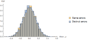
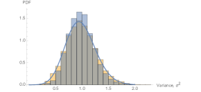
Figure 8: Distribution of $\hat{\mu}$ and $\hat{\sigma}^{2}$ from $10^{4}$ MC simulations. Orange shows the original experiment with only the same errors, while blue shows the distribution with errors $\sigma_{i}$ distributed uniformly between $0.1$ to $1.9$. We see clearly that while the distribution of the mean is more or less unchanged, the distribution of $\hat{\sigma}^{2}$ is altered, and no longer follows the $\chi^{2}$ distribution derived earlier. The two histograms have the expected distribution for the original experiment superimposed.

Another interesting distribution to see from this experiment is the distribution of the $\chi^{2}=\sum(\hat{x}_{i}-\hat{\mu})^{2}/(\sigma^{2}+\sigma_{i}^{2})$. This is shown in Fig. 9. It is immediate that the $\chi^{2}$ distribution does not describe this distribution very well. We can interpret this as exchanging variability is the $\chi^{2}$ for variability in the $\hat{\sigma}^{2}$. Had we set all $\sigma_{i}^{2}\ll\sigma^{2}$, then we end up with the situation from Sec. 2.4.2, and the $\chi^{2}$ is always perfect, and all variability is in the $\sigma^{2}$. If we instead have $\sigma_{i}^{2}\gg\sigma^{2}$, then all the errors are practically fixed and we end up with an almost linear model, ie. the $\sigma^{2}$ does nothing to the fit, and we just fit $\mu$. This gives us a fixed $\sigma\approx 0$ and a $\chi^{2}$ which is distributed, well, as a $\chi^{2}$. The situation here is a kind of middle ground, where both are of the same order, and so the $\chi^{2}$ holds some of the variation, while also the $\hat{\sigma}^{2}$ varies.

Most importantly, this shows that when the errors on the datapoints are not equal, the MLE is not always a perfect fit, ie. $\chi^{2}\neq N$. Even when fitting the error, some variation remains.

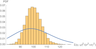
Figure 9: Distribution of $\chi^{2}=\sum(\hat{x}_{i}-\hat{\mu})^{2}/(\sigma^{2}+\sigma_{i}^{2})$ from MC simulations with distinct errors. Superimposed is a $\chi^{2}$ distribution with $100$ degrees of freedom.

These two examples show the very basics of MC simulations, and the types of problems they solve. This section is by no means exhaustive. It is mostly meant as a very soft introduction to the subject of stuff we can’t calculate exactly, which unfortunately is a very big one.

2.6   Bayesian statistics

All statistical analysis in our work is frequentist. An objection to what I have shown so far, as I already mentioned, is that the p-values we get out are not probabilities in the sense we would like them to be — they do not represent model probabilities. If one is unsatisfied by this, then we may use Bayes’ theorem to go from the likelihood, which is the pdf of data given a model, to a posterior pdf, say $f(\theta|\hat{X})$, which is the probability of a certain model given the obtained data. By Eq. (2.1.2), this is done as

$$f(\theta|\hat{X})=\frac{\mathcal{L}(\theta)f(\theta)}{f(\hat{X})}$$ (2.6.1)

where, given $f(\theta)$, $f(\hat{X})=\int\mathcal{L}(\theta)f(\theta)\ d\theta$. $f(\theta)$ is called the prior, and $f(\hat{X})$ is called the evidence. Note however, that using Bayes’ theorem requires a prior, for which we in most cases of interest in fundamental physics have no idea what should be. In particular, the pdf changes under change of variables, so if we were to pick something boring, in the sense of being uninformative, then the very same function in another variable might be very restrictive — recall the discussion in Sec. 2.4.5.

With Bayesian statistics, we get exactly what we like — a direct measure of the pdf of a model given the data we see. No hypothesis testing and no ambiguous p-values. The price one has to pay is the choice of a prior, which in some cases is less trivial than other. In a sense, the Bayesian method is trying to answer the unanswerable — doing fundamental physics, there is no way we can pick the true prior, since all our knowledge on any subject is derived from experience, which again would have to have been interpreted with some prior.

Cosmology

Today’s cosmological studies are by and large interpreted within the bounds of the so-called Concordance or Standard cosmological model. In this section, I will give a summary of the theory with some examples of links to observables and experiments constraining it. I cannot hope to give a textbook introduction to cosmology, but instead refer to one of the many excellent books written on the subject, [9, 10, 11, 12].

3.1   General relativity

The foundation of modern cosmology is Einstein’s general theory of relativity. Here I aim to introduce main motivations and concepts necessary for the framework of cosmology. This describes not only how matter moves in space and time, but also how matter influences, or perhaps more famously bends, spacetime.

The geometry of spacetime is described by the metric, which tells the distance between neighbouring points. We define the proper time interval as

$$d\tau^{2}\equiv-g_{\mu\nu}dx^{\mu}dx^{\nu},$$ (3.1.1)

which defines for us the metric. The equations of motion for a test-particle in spacetime is, in a freely falling, locally inertial coordinate system, a straight line, or more specifically a curve of extremal proper time. In this coordinate system, call it $\xi$, this means we differentiate the coordinates of the particle two times with respect to the proper time and require it be zero,

$$\frac{\partial^{2}\xi^{\mu}}{\partial\tau^{2}}=0.$$ (3.1.2)

By reparametrisation invariance — loosely the statement that Nature doesn’t care what coordinates we use — we can translate the coordinates $\xi$ to any coordinate system $x$ we find convenient, leaving all physics invariant. In particular, the line-element Eq. (3.1.1) doesn’t change,

$$-\eta_{\mu\nu}d\xi^{\mu}d\xi^{\nu}=-g_{\mu\nu}dx^{\mu}dx^{\nu}$$ (3.1.3)

In the $\xi$ coordinates, the metric takes the very special form $\eta=diag(-1,1,1,1)$. In the $x$ coordinates Eq. (3.1.2) takes the form

$$\frac{\partial}{\partial\tau}\left(\frac{\partial\xi^{\mu}}{\partial x^{\nu}}\frac{\partial x^{\nu}}{\partial\tau}\right) =\frac{\partial\xi^{\mu}}{\partial x^{\nu}}\frac{\partial^{2}x^{\nu}}{\partial\tau^{2}}+\frac{\partial^{2}\xi^{\mu}}{\partial x^{\nu}\partial x^{\rho}}\frac{\partial x^{\nu}}{\partial\tau}\frac{\partial x^{\rho}}{\partial\tau}=0$$

$$\Rightarrow\frac{\partial^{2}x^{\mu}}{\partial\tau^{2}}+\Gamma^{\mu}_{\rho\sigma}\frac{\partial x^{\rho}}{\partial\tau}\frac{\partial x^{\sigma}}{\partial\tau}=0$$ (3.1.4)

where the second line follows from multiplying with $\frac{\partial x^{\lambda}}{\partial\xi^{\mu}}$ and renaming indices. I also introduce the affine connection

$$\Gamma^{\mu}_{\rho\sigma}\equiv\frac{\partial^{2}\xi^{\nu}}{\partial x^{\rho}\partial x^{\sigma}}\frac{\partial x^{\mu}}{\partial\xi^{\nu}}$$ (3.1.5)

$$\Rightarrow\frac{\partial^{2}\xi^{\lambda}}{\partial x^{\rho}\partial x^{\sigma}}=\frac{\partial\xi^{\lambda}}{\partial x^{\mu}}\Gamma^{\mu}_{\rho\sigma}$$ (3.1.6)

Eq. (3.1) is known as the geodesic equation.

There is a subtlety here, which I brushed over. For massless particles — radiation — we cannot use the proper time as independent variable to label the path, since this vanishes identically. Instead use the zero-component of the coordinate vector, $\xi^{0}$. The following derivation is like before and we end up with

$$0=\frac{\partial^{2}x^{\mu}}{\partial(\xi^{0})^{2}}+\Gamma^{\mu}_{\rho\sigma}\frac{\partial x^{\rho}}{\partial\xi^{0}}\frac{\partial x^{\sigma}}{\partial\xi^{0}}$$ (3.1.7)

We will need these equations to describe the propagation and properties of particles in the universe. Before doing that, we must know how spacetime reacts to matter. First, let’s rewrite the connection. Rewrite Eq. (3.1.3)

$$g_{\mu\nu}=\frac{\partial\xi^{\alpha}}{\partial x^{\mu}}\frac{\partial\xi^{\beta}}{\partial x^{\nu}}\eta_{\alpha\beta}$$ (3.1.8)

and differentiate with respect to the $x$ coordinates

$$\frac{\partial g_{\mu\nu}}{\partial x^{\lambda}} =\left\{\frac{\partial^{2}\xi^{\alpha}}{\partial x^{\mu}\partial x^{\lambda}}\frac{\partial\xi^{\beta}}{\partial x^{\nu}}+\frac{\partial\xi^{\alpha}}{\partial x^{\mu}}\frac{\partial^{2}\xi^{\beta}}{\partial x^{\nu}\partial x^{\lambda}}\right\}\eta_{\alpha\beta}$$

$$=\left\{\Gamma^{\sigma}_{\mu\lambda}\frac{\partial\xi^{\alpha}}{\partial x^{\sigma}}\frac{\partial\xi^{\beta}}{\partial x^{\nu}}+\frac{\partial\xi^{\alpha}}{\partial x^{\mu}}\Gamma^{\sigma}_{\nu\lambda}\frac{\partial\xi^{\beta}}{\partial x^{\sigma}}\right\}\eta_{\alpha\beta}$$

$$=\Gamma^{\sigma}_{\mu\lambda}g_{\sigma\nu}+\Gamma^{\sigma}_{\nu\lambda}g_{\sigma\mu},$$ (3.1.9)

where line 2 and 3 follow from Eq. (3.1.6) and Eq. (3.1.8) respectively. Next, add three of these with mixed indices,

$$\frac{\partial g_{\mu\alpha}}{\partial x^{\nu}}+\frac{\partial g_{\nu\alpha}}{\partial x^{\mu}}-\frac{\partial g_{\mu\nu}}{\partial x^{\alpha}} =\Gamma^{\sigma}_{\mu\nu}g_{\sigma\alpha}+\Gamma^{\sigma}_{\alpha\nu}g_{\sigma\mu}$$

$$+\Gamma^{\sigma}_{\nu\mu}g_{\sigma\alpha}+\Gamma^{\sigma}_{\alpha\mu}g_{\sigma\nu}$$

$$-\Gamma^{\sigma}_{\mu\alpha}g_{\sigma\nu}-\Gamma^{\sigma}_{\nu\alpha}g_{\mu\sigma}$$

$$=2\Gamma^{\sigma}_{\mu\nu}g_{\sigma\alpha},$$ (3.1.10)

where I use that the connection is symmetric in the two lower indices, as is clear from the definition Eq. (3.1.5). Defining the inverse of the metric, $g^{\mu\nu}$,

$$g^{\mu\nu}g_{\nu\lambda}=\delta^{\mu}_{\lambda}$$ (3.1.11)

we multiply Eq. (3.1.10) by $g^{\lambda\alpha}$ and get

$$\Gamma^{\lambda}_{\mu\nu}=\frac{1}{2}g^{\lambda\alpha}\left\{\frac{\partial g_{\mu\alpha}}{\partial x^{\nu}}+\frac{\partial g_{\nu\alpha}}{\partial x^{\mu}}-\frac{\partial g_{\mu\nu}}{\partial x^{\alpha}}\right\}$$ (3.1.12)

This expression is entirely free from the coordinates $\xi$, and can be readily calculated given the metric $g^{\mu\nu}$ in any coordinate system.

Now we want to write tensors describing the spacetime. Using just the metric and its first and second derivatives, one can show that the unique tensor which is linear in second derivatives of the metric, is the Riemann(-Christoffel curvature-)tensor,

$$R^{\lambda}_{\mu\nu\rho}=\frac{\partial\Gamma^{\lambda}_{\mu\rho}}{\partial x^{\nu}}+\frac{\partial\Gamma^{\lambda}_{\mu\nu}}{\partial x^{\rho}}+\Gamma^{\lambda}_{\rho\eta}\Gamma^{\eta}_{\mu\nu}+\Gamma^{\lambda}_{\nu\eta}\Gamma^{\eta}_{\mu\rho}$$ (3.1.13)

Of course we can also take contractions of this tensor, of which the two we will need are the Ricci tensor,

$$R_{\mu\nu}=R^{\lambda}_{\mu\lambda\nu}$$ (3.1.14)

and the curvature scalar

$$R=R^{\mu}_{\mu}$$ (3.1.15)

In general, a non-vanishing Riemann tensor signifies the presence of a gravitational field. If the Riemann tensor is strictly zero, then some transformation takes one back to Minkowski space, which has the metric $\eta_{\mu\nu}$. Any non-zero component of the Riemann tensor prohibits such a transformation. With these tensors, Einstein’s field equations (EFE) take the form

$$R_{\mu\nu}-\frac{1}{2}g_{\mu\nu}R-\Lambda g_{\mu\nu}=-8\pi GT_{\mu\nu},$$ (3.1.16)

$$\Leftrightarrow R_{\mu\nu}=-8\pi G\left(T_{\mu\nu}-\frac{1}{2}T^{\lambda}_{\lambda}g_{\mu\nu}\right)-\Lambda g_{\mu\nu}$$ (3.1.17)

where $T_{\mu\nu}$ is the energy stress tensor, $G=6.67\cdot 10^{-11}\text{Nm}^{2}\text{/kg}^{2}$ is Newton’s constant and $\Lambda$ is the infamous Cosmological Constant. I return to this in Sec. 3.4. The second equation above follows from tracing the first.

Newtonian mechanics   As everyone learned in school, Newton predicted the trajectories of planets, combining his $F\propto r^{-2}$ law of gravity with $F=ma$. Let’s see how this is the limiting case of the geodesic equation and a specific geometry — as of course it should be.

The limit we will take is a stationary weak field, and a slowly moving test particle. This translates to the following expressions

$$g_{\mu\nu}=\eta_{\mu\nu}+h_{\mu\nu}$$ (3.1.18)

$$|h_{\mu\nu}|\ll 1$$ (3.1.19)

$$\frac{\partial h_{\mu\nu}}{\partial t}=0$$ (3.1.20)

$$\left|\frac{\partial t}{\partial\tau}\right|\gg\left|\frac{\partial x^{i}}{\partial\tau}\right|$$ (3.1.21)

Using Eq. (3.1.21), we write the geodesic equation (3.1) as

$$\frac{\partial^{2}x^{\mu}}{\partial\tau^{2}}=\Gamma^{\mu}_{00}\left(\frac{\partial t}{\partial\tau}\right)^{2}$$ (3.1.22)

Calculating the connection, we use that all time derivatives of the metric vanish, and derivatives only act on the small, $h$-part. To first order in $h$ we have

$$\Gamma^{\mu}_{00}=-\frac{1}{2}g^{\mu\nu}\frac{\partial g_{00}}{\partial x^{\nu}}=-\frac{1}{2}\eta^{\mu\nu}\frac{\partial h_{00}}{\partial x^{\nu}}$$ (3.1.23)

Putting this into Eq. (3.1.22) we get,

$$\frac{\partial^{2}t}{\partial\tau^{2}} =0$$ (3.1.24)

$$\frac{\partial^{2}x}{\partial\tau^{2}} =\frac{1}{2}\left(\frac{\partial t}{\partial\tau}\right)^{2}\nabla h_{00}\Rightarrow\frac{\partial^{2}x}{\partial t^{2}}=\frac{1}{2}\nabla h_{00}$$ (3.1.25)

This looks an awful lot like the Newtonian result,

$$ma=-m\nabla\phi$$ (3.1.26)

where $\phi$ is some Newtonian potential. For eg. a spherical mass distribution of mass $M$, this takes the familiar form $\phi=-GM/r$. We see that setting $h_{00}=-2\phi$ gives us the Newtonian solution. To check that our approximation holds for typical potentials, put in values for the Sun- and Earth-radius and mass,

$$|\phi_{\text{Sun}}|=\frac{GM_{\text{Sun}}}{R_{\text{Sun}}}=2.12\cdot 10^{-6}$$ (3.1.27)

$$|\phi_{\text{Earth}}|=\frac{GM_{\text{Earth}}}{R_{\text{Earth}}}=6.95\cdot 10^{-10}$$ (3.1.28)

Evidently the approximation is very good even at astrophysical scales!

3.2   The cosmological principle

The EFE are in general very hard to solve. Given $T_{\mu\nu}$, they describe 10 coupled partial differential equations for the metric $g_{\mu\nu}$. As such, any exact solution typically has a lot of simplifying symmetry. The cosmological principle is one such set of symmetries. In short, it states that our or anyone else’s place and orientation in the universe shouldn’t be special. Any translation or rotation must therefore leave the metric invariant. Obviously, the universe isn’t exactly homogeneous or isotropic. These properties are meant to be approximately true only on cosmological scales, meaning when we average matter and geometry over large enough scales, this description is suitable.

This high degree of symmetry forces the line element (3.1.1) to take the form

$$d\tau^{2}=dt^{2}-a(t)^{2}\left(\frac{dr^{2}}{1-kr^{2}}+r^{2}d\Omega^{2}\right)$$ (3.2.1)

where $d\Omega^{2}=d\theta^{2}+d\phi^{2}\cos^{2}\theta$ and $k\in\{-1,0,+1\}$. The different signs of $k$ correspond to an open, flat and closed universe, respectively. The metric is known as the Friedmann-Lemaître-Robertson-Walker (FLRW) metric. The function $a(t)$ is some so far unspecified function of cosmic time $t$, called the scale factor. To find this function, we must solve the EFE. The source must also be maximally symmetric in space, and so takes the form of a perfect fluid,

$$T_{\mu\nu}=pg_{\mu\nu}+(p+\rho)U_{\mu}U_{\nu},$$ (3.2.2)

where $p$ and $\rho$ are the pressure and energy density of the fluid, and $U$ is the fluid velocity, which in the cosmic rest-frame is given by

$$U^{0}=1$$

$$U^{i}=0,$$

that is to say, the contents of the universe are, on cosmological scales, relatively quiet. Because of the high degree of symmetry in the problem, only two independent equations remain of the EFE. The first is the Friedman equation,

$$\dot{a}^{2}+k=\left(\frac{8\pi G}{3}\rho+\frac{\Lambda}{3}\right)a^{2}$$ (3.2.3)

and the second I take as conservation of energy, and write as

$$\frac{d}{da}(\rho a^{3})+3pa^{2}=0$$ (3.2.4)

To close the set of equations, we need an equation of state, describing the pressure as a function of the energy density

$$p=p(\rho)$$ (3.2.5)

Two equations of state are of particular importance. These are of non-relativistic matter, or dust, and ultra-relativistic matter, or equivalently, radiation. The two are

$$p_{\text{matter}}\ll\rho$$ (3.2.6)

$$p_{\text{radiation}}=\rho/3$$ (3.2.7)

For the two we find, according to Eq. (3.2.4) the dilution of the energy density is

$$\rho_{\text{matter}}\propto a^{-3}$$ (3.2.8)

$$\rho_{\text{radiation}}\propto a^{-4}$$ (3.2.9)

These factors should not come as a surprise. Thinking in terms of an expanding universe, matter is simply spread over greater volumes and dilutes as $1/V$, whereas radiation is not only diluted, but also stretched by the expansion. One can in general think of some perfect fluid with equation of state

$$p=w\rho.$$ (3.2.10)

I will in the following keep the radiation and matter factors explicit, but all calculations can be made with arbitrary $w$.

With these expression for the energy density, we can in principle solve the Friedmann equation. It is customary to rewrite the equation a bit. First introduce the Hubble parameter and critical density,

$$H =\dot{a}/a,\hskip 28.45274ptH_{0}=H(\text{today})=100h\frac{\text{km}}{\text{s}\cdot\text{Mpc}}$$ (3.2.11)

$$\rho_{c} =\frac{3H_{0}^{2}}{8\pi G}.$$ (3.2.12)

Dividing Eq. (3.2.3) through by $a^{2}$ we get

$$H^{2}=H_{0}^{2}\left(\frac{\rho}{\rho_{c}}+\frac{\Lambda}{3H_{0}^{2}}-\frac{k}{a^{2}H_{0}^{2}}\right)$$ (3.2.13)

The density $\rho$ can now be matter, radiation or both. Taking into account how the two densities scale, write

$$\rho=\rho_{m}+\rho_{R}=\frac{a_{0}^{3}}{a^{3}}\rho_{m0}+\frac{a_{0}^{4}}{a^{4}}\rho_{R0}$$ (3.2.14)

where $a_{0}=a(t=t_{0})$ is the scale factor today. Now define the density parameters $\Omega_{i}$ as

$$\Omega_{m} =\frac{\rho_{M0}}{\rho_{c}},\hskip 28.45274pt\Omega_{R}=\frac{\rho_{R0}}{\rho_{c}}$$

$$\Omega_{\Lambda} =\frac{\Lambda}{3H_{0}^{2}},\hskip 28.45274pt\Omega_{k}=-\frac{k}{a_{0}^{2}H_{0}^{2}}$$ (3.2.15)

and finally, write the Friedmann equation as

$$H^{2}=H_{0}^{2}\left\{\Omega_{m}(a/a_{0})^{-3}+\Omega_{R}(a/a_{0})^{-4}+\Omega_{\Lambda}+\Omega_{k}(a/a_{0})^{-2}\right\}$$ (3.2.16)

Inserting $t=t_{0}$ we easily see that the density parameters obey the sum rule

$$\Omega_{m}+\Omega_{R}+\Omega_{\Lambda}+\Omega_{k}=1$$ (3.2.17)

Widely accepted, concordance, values for the values of these parameters in the present universe are ([13])

$$\Omega_{m} \approx 0.3\hskip 28.45274pt\Omega_{R}\approx 0$$

$$\Omega_{\Lambda} \approx 0.7\hskip 28.45274pt\Omega_{k}\approx 0$$

$$H_{0} \approx 70\text{Mpc}^{-1}\text{km/s}\approx 1.3\cdot 10^{-41}\text{GeV}$$ (3.2.18)

which is why the current setting is called $\Lambda$CDM. $\Lambda$ for a Cosmological Constant, CDM for cold dark matter. The actual baryonic matter we are all made of is in this picture a mere $5\%$, which is included in the $\Omega_{m}$ here.

Single component universes   For the sake of intuition, let’s work through some examples of single component universes. In particular, consider the four immediate possibilities — matter, radiation, curvature, and Cosmological Constant-dominated universes, with each of the four density parameters $\Omega_{i}=1$ and all others $0$. This corresponds to solving the equation

$$\frac{\dot{a}}{a}=\frac{\dot{a}_{0}}{a_{0}}\left(\frac{a}{a_{0}}\right)^{-n/2}\Rightarrow\frac{\dot{a}}{\dot{a}_{0}}=\left(\frac{a}{a_{0}}\right)^{1-n/2}$$ (3.2.19)

for $n\in\{3,4,2,0\}$, respectively. Assume now a power-law form, $a\propto t^{m}$. Putting this in our equation, we get the condition

$$m=\frac{2}{n},\ \ \ n\neq 0$$ (3.2.20)

For the Cosmological Constant, this solution fails, but we see immediately for $n=0$ the answer must be an exponential function. For the four different single component universes we have the following solutions

$$a(t)=a_{0}\times\left\{\begin{matrix}\left(\frac{t}{t_{0}}\right)^{2/3}&\text{matter dominated (Einstein-de Sitter) }\\ \left(\frac{t}{t_{0}}\right)^{1/2}&\text{radiation dominated }\\ t/t_{0}&\text{curvature dominated (Milne) }\\ \exp(H_{0}t)&\text{Cosmological Constant dominated (de Sitter)}\end{matrix}\right.$$ (3.2.21)

Finally, extrapolating $a\rightarrow 0$, we get the following expressions for the age of the universe in terms of the present Hubble constant,

$$t_{a=0}=\frac{1}{H_{0}}\times\left\{\begin{matrix}2/3&\text{matter dominated (Einstein-de Sitter) }\\ 1/2&\text{radiation dominated }\\ 1&\text{curvature dominated (Milne) }\\ \infty&\text{Cosmological Constant dominated (de Sitter)}\end{matrix}\right.$$ (3.2.22)

Since we observe neither cosmic time, nor the absolute scale factor, it would be nice to have a proxy for the two. To this end, we introduce the cosmological redshift, denoted $z$. This is the fractional amount the wavelength of radiation has been stretched by the universe expanding. To see how this comes about, place an observer at $r=0$ and let a wave crest be emitted at $t_{1}$ propagating radially inwards from some radius $r_{1}$. For a lightlike test particle, the proper time is zero, and we have

$$0=dt^{2}-a(t)^{2}\frac{dr^{2}}{1-kr^{2}}$$ (3.2.23)

Call the time it is observed $t_{0}$, we then have the equation

$$\int_{t_{1}}^{t_{0}}\frac{dt}{a(t)}=\int_{0}^{r_{1}}\frac{dr}{\sqrt{1-kr^{2}}}=\frac{1}{\sqrt{k}}\sin^{-1}(\sqrt{k}r_{1})$$ (3.2.24)

Notice the sign in taking the square root is fixed by the direction of propagation. The next wave crest is emitted shortly after, follows the same path and obeys the same equation but with slightly shifted time coordinates,

$$\int_{t_{1}+1/\nu_{1}}^{t_{0}+1/\nu_{0}}\frac{dt}{a(t)}=\frac{1}{\sqrt{k}}\sin^{-1}(\sqrt{k}r_{1}),$$ (3.2.25)

where $\nu_{i}$ is the frequency at $r_{i}$. For frequencies much larger than $H\approx 3.2\cdot 10^{-18}h\text{s}^{-1}$ we get

$$0= \int_{t_{1}}^{t_{0}}\frac{dt}{a(t)}-\int_{t_{1}+1/\nu_{1}}^{t_{0}+1/\nu_{0}}\frac{dt}{a(t)}\approx\frac{1}{a(t_{1})\nu_{1}}-\frac{1}{a(t_{0})\nu_{0}}$$

$$\Rightarrow \hskip 28.45274pt\frac{\nu_{1}}{\nu_{0}}=\frac{a(t_{0})}{a(t_{1})}$$ (3.2.26)

We now define the redshift as the fractional increase in wavelength,

$$z=\frac{\lambda_{0}-\lambda_{1}}{\lambda_{1}}=\frac{\nu_{1}}{\nu_{0}}-1=\frac{a(t_{0})}{a(t_{1})}-1$$ (3.2.27)

This is a nice quantity to work with because it is readily observable through analyses of spectra. We can rewrite Eq. (3.2.16) trading $t$ and $a$ for $z$, giving

$$H(z)^{2}=H_{0}^{2}\left\{\Omega_{m}(1+z)^{3}+\Omega_{R}(1+z)^{4}+\Omega_{\Lambda}+\Omega_{k}(1+z)^{2}\right\}$$ (3.2.28)

3.3   Cosmography

On cosmological scales, the intuitive notion of distances fails. Depending on the question you ask, distances to the same object may differ — by a lot. In this section, I explore the different measures of distance and try to clarify their meaning.

First, let us connect the $r$ coordinate to the physical redshift. Take an observer and an emitter, say a galaxy or a supernova, at relative proper distance $r_{1}$. Emitting a single photon at $t=t_{1}$, we observe it at $t=t_{0}$. The photon follows the path described in Eq. (3.2.23), and upon inverting Eq. (3.2.24) we get, with a change of variables,

$$r_{1}=\frac{1}{\sqrt{k}}\sin\left(\frac{\sqrt{k}}{a_{0}}\int_{0}^{z}\frac{dz^{\prime}}{H(z^{\prime})}\right).$$ (3.3.1)

Usually though, a single photon is not enough. What we might hope to measure is a stream of light from a source of known luminosity. Considerations from Euclidian space lead us to define the luminosity distance, $d_{L}$ as

$$F=\frac{L}{4\pi d_{L}^{2}},$$ (3.3.2)

where $F$ is the measured flux from an object of luminosity $L$. Now we seek the relation between this definition and the proper distance — and hence the redshift. Note that $F$ and $L$ are bolometric quantities, ie. integrated over all frequencies. First, consider the area over which the emitted light is spread. Integrating the angular part of the metric, we get a total area, at time $t_{0}$ — when the light is observed

$$A=4\pi a(t_{0})r_{1}.$$ (3.3.3)

Travelling across the universe has its price, though. First, the emitted light is redshifted, which reduces the energy per observed photon by one factor $(1+z)$, and second, the distance between individual photons is increased, also by a factor $(1+z)$. This means the observed flux is reduced by a total factor $(1+z)^{2}$, giving

$$F=\frac{L}{4\pi a(t_{0})^{2}r_{1}^{2}(1+z)^{2}}\Rightarrow d_{L}=(1+z)a(t_{0})r_{1}.$$ (3.3.4)

Next we look at an object or a feature, which is extended across the sky in some angle $\delta\theta\ll 1$ at proper distance $r_{1}$. Looking again to Euclidean geometry, we expect the measured angle to be the length of the object, $D$, divided by the distance $d_{A}$,

$$\delta\theta=\frac{D}{d_{A}}$$ (3.3.5)

To find the relation between the angular diameter distance and the proper distance, we arrange our coordinate system appropriately and integrate only $\theta$ in the metric. Doing this we get that the proper distance between the two ends of the object at $t_{1}$ is

$$D=a(t_{1})r_{1}\delta\theta\Rightarrow d_{A}=a(t_{1})r_{1}=(1+z)^{-1}a(t_{0})r_{1}.$$ (3.3.6)

An equivalent definition in terms the solid angle $\delta\Omega$, filled by an object of proper area $\delta A$ is

$$d_{A}=\sqrt{\frac{\delta A}{\delta\Omega}}$$ (3.3.7)

The transverse comoving distance is defined as the ratio of the proper transverse motion of a particle to the angular motion we see

$$d_{M}=\frac{\Delta D/\delta t_{1}}{\delta\theta/\delta t_{0}}=d_{A}(1+z)=a_{0}r_{1}.$$ (3.3.8)

Note that it is not, as the angular diameter distance, the physical length of an object.

Curved space   To gain a bit of intuition for curved space, consider measuring $d_{M}$. Without looking to the equations, we ask ourselves ”are we going to measure more or less than we think?”. Recall that in positively curved space, parallel lines get closer and closer, while in negatively curved space, they grow further apart — the first point is most easily seen by imagining a 2-sphere, where lines that are parallel at and orthogonal to the equator will intersect at the poles. Now, we observe some angle, which is to say at our position, the two lines going to each of the two sources we observe have some incident angle at our position. As we just argued, the separation between two lines changes in curved space compared to flat space. This means that in positively curved space, the two lines going to the two sources will get closer as they go along, and the distance $d_{M}$ is smaller than in flat space. Conversely, in negatively curved space, the lines get further apart and $d_{M}$ is larger, see Fig. 10. This effect is exactly the effect of the $\sin$ function in the expression Eq. (3.3.1).

Figure 10: Sketch of lines with equal incident angle at the observer point, propagating in differently curved spaces. From outside in, the universes have $k=-1,0,+1$. This shows how the distance measured is affected by the curvature of space, as the length between the lines at the top — at the source position — is changed by the warping of the geodesics.

We see that the angular diameter distance and luminosity distance are not independent from the proper distance — they satisfy the Etherington reciprocity relation,

$$d_{A}(1+z)=d_{M}=d_{L}(1+z)^{-1}$$ (3.3.9)

We finally want to know what part of the universe can ever have had an effect at our position, given that the current dynamics are what have always been at play. That is, at a given time in the history of the universe, how big was the causally connected part. The proper distance to this horizon is just the integral of the square root of the radial part of the metric

$$d_{H}=a(t)\int_{0}^{r_{H}}\frac{dr}{\sqrt{1-kr^{2}}}=a(t)\int_{0}^{t}\frac{dt^{\prime}}{a(t^{\prime})}$$ (3.3.10)

The horizon problem   Consider a matter-dominated universe, which for the following calculation will simulate the universe we live in. Calculating the distance to the horizon is straight-forward, and we get

$$d_{H,\text{matter}}=\frac{2}{H_{0}}(1+z)^{-3/2}.$$ (3.3.11)

Watching this horizon on the sky from far away, we expect that any two points further apart than $d_{H}$ will not be in causal contact — and will not a priori know anything about one another. Let’s calculate the size on the sky of such a horizon patch. The angular diameter distance is in the matter dominated universe given by

$$d_{A,\text{matter}}=\frac{2}{H_{0}}\frac{1-(1+z)^{-1/2}}{1+z}$$ (3.3.12)

The angular size of the patch for a given redshift is then

$$\delta\theta=d_{H}/d_{A}$$ (3.3.13)

The cosmic microwave background (CMB) radiation is the leftover thermal bath of photons from the early universe. The photons decoupled at redshift $1+z\approx 1100$ and have been free streaming since then. The size of a horizon patch at this decoupling redshift is

$$\delta\theta\approx\frac{1100^{-1/2}}{1-1100^{-1/2}}=0.031\text{rad}=1.8^{o}$$ (3.3.14)

Note that this is significantly less than $180^{o}$. This means that patches on the sky separated by more than $1.8^{o}$ should be completely independent — the exact number changes slightly for different universes, but the point remains. The great surprise is the fact that the temperature of these photons is to very high precision constant over the whole sky. This means that apparently, the entire observed universe has been in causal constant at some point, yet our calculations show, that given the present expansion of the universe, there is no way it could have been. This is known as the horizon problem. One solution to this problem — inflation — is to insert a sudden de Sitter period, which blows up the horizon, while keeping the Hubble parameter constant. This can leave the observed universe inside the horizon distance. The problem is of course formulated assuming the metric description holds to $t=0$, in order that the integral (3.3.10) can be calculated.

For distances at low redshift, $z\ll 1$, we can expand the expressions previous and do the integrals. I will illustrate this with the luminosity distance, and on the way introduce the deceleration parameter. Take the expression Eq. (3.3.4) and taylor expand the integral of in $r_{1}$. Since $\sin(x)=x+\mathcal{O}(x^{3})$, we can get to second order in $z$ while just considering the expression

$$H_{0}d_{L}= (1+z)\int_{0}^{z}\frac{dz^{\prime}}{\sqrt{\Omega_{m}(1+z)^{3}+\Omega_{\Lambda}+(1-\Omega_{m}-\Omega_{\Lambda})(1+z)^{2}}}$$

$$= (1+z)\left(z-\frac{z^{2}}{2}(1-q_{0})+\mathcal{O}(z^{3})\right),\hskip 28.45274ptq_{0}\equiv\Omega_{m}/2-\Omega_{\Lambda}$$ (3.3.15)

where $q_{0}$ is the deceleration parameter, and I have ignored radiation, as is justified in the late universe. This measures the degree to which the universe is decelerating — named so since historically it was believed the universe was decelerating and positive numbers are pleasing. Let’s see how the acceleration of the FRW universe is related to this parameter. We turn to the expansion of the scale factor around the present time, $t-t_{0}\ll H_{0}^{-1}$,

$$a(t) =a_{0}+\dot{a}_{0}(t-t_{0})+\frac{\ddot{a}_{0}}{2}(t-t_{0})^{2}+\mathcal{O}(t^{3})$$

$$=a_{0}\left(1+[t-t_{0}]H_{0}-\frac{1}{2}\left(-\frac{\ddot{a}_{0}a_{0}}{\dot{a}_{0}^{2}}\right)([t-t_{0}]H_{0})^{2}+\mathcal{O}(t^{3})\right)$$ (3.3.16)

The coefficient in front of the second order term is just what we’re looking for. To see this, reorder and differentiate the Friedmann equation, (3.2.16) with respect to time,

$$\frac{\partial}{\partial t}\dot{a} =\frac{\partial}{\partial t}H_{0}a\sqrt{\Omega_{m}(a/a_{0})^{-3}+\Omega_{\Lambda}+\Omega_{k}(a/a_{0})^{-2}}$$

$$\Rightarrow\ddot{a} =H_{0}\dot{a}\left(\sqrt{\Omega_{m}(a/a_{0})^{-3}+\Omega_{\Lambda}+\Omega_{k}(a/a_{0})^{-2}}\right.$$

$$\left.+\frac{-3\Omega_{m}(a/a_{0})^{-3}-2\Omega_{k}(a/a_{0})^{-2}}{2\sqrt{\Omega_{m}(a/a_{0})^{-3}+\Omega_{\Lambda}+\Omega_{k}(a/a_{0})^{-2}}}\right)$$

$$\Rightarrow\ddot{a}_{0} =H_{0}\dot{a}_{0}\left(1+\frac{-2-\Omega_{m}+2\Omega_{\Lambda}}{2}\right)=-H_{0}\dot{a}_{0}\left(\Omega_{m}/2-\Omega_{\Lambda}\right)$$

$$\Rightarrow-q_{0} =\frac{\ddot{a}_{0}a_{0}}{\dot{a}_{0}^{2}}.$$ (3.3.17)

We can see $q_{0}$ as a scale-free measure of the deceleration of the universe — the scale of expansion is set by $H_{0}$ and the scale of the universe by $a_{0}$. Note that $q_{0}$ only describes the deceleration of the universe today. Generally, $q$ changes throughout the course of the universe. Only in very special cases the universe is forever non-accelerating.

3.3.1   Moving emitter and observers

The Doppler effect, being a well established phenomenon, also has to be taken into account when measuring the universe. Typical peculiar velocities of galaxies, which is to say the velocity in excess of the Hubble recession, are expected to be of the order a few hundred kilometers per second, ie. $v\approx 10^{-3}$ in units of the speed of light. This includes both us as observers and eg. SNe as emitters. The problem I wish to address in the present subsection is what difference this makes to the light we receive. Now, since these velocities are only mildly relativistic, we shall only look at the first term in an expansion around zero velocity. The following derivation follows the work in [14].

First we realise that the redshift we see is not only redshifted by the expanding universe, but also by normal relativistic Doppler shifting. Denoting the expected redshift in a completely still universe by $z$ as before, we write $\bar{z}$ for the corrected redshift in the universe where everyone is moving around. By normal Doppler shifting, $\bar{z}$ is given by

$$1+\bar{z}=(1+z)(1+n\cdot[v_{e}-v_{o}])+\mathcal{O}(v^{2})$$ (3.3.18)

where the $v_{i}\ll 1$ are the velocities of the emitter and observer, respectively, and $n$ is a unit vector point from the observer to the emitter. From here onwards, anything but the first $v_{i}$ term is neglected. Now, beaming effects also come into play, in particular the solid angle of the emitter is changed by relativistic beaming as

$$\delta\Omega\rightarrow\delta\Omega(1-2n\cdot v_{o})$$ (3.3.19)

Note that this only depends on the observer-velocity, not the emitter. This changes the angular diameter distance, Eq. (3.3.7), which we can in turn link to the luminosity distance through Eq. (3.3.9). We see that the changes are the following

$$\bar{d}_{A}(\bar{z}) =d_{A}(z)(1+n\cdot v_{o})$$ (3.3.20)

$$\Rightarrow\bar{d}_{L}(\bar{z}) =d_{L}(z)(1+n\cdot v_{o})\frac{(1+\bar{z})^{2}}{(1+z)^{2}}\approx d_{L}(z)(1+n\cdot[2v_{e}-v_{o}])$$ (3.3.21)

We are still not done yet, as this last equation does not relate directly observable quantities. The redshift we observe is naturally $\bar{z}$, so we will have to also evaluate $d_{L}$ at this slightly shifted redshift. What I will do is a simple Taylor expansion of the function. This means we take

$$d_{L}(z)=d_{L}(\bar{z})+\frac{\partial d_{L}(\bar{z})}{\partial z}(z-\bar{z}),$$ (3.3.22)

where we can write $z-\bar{z}=-(1+\bar{z})n\cdot[v_{e}-v_{o}]$, and so we just miss the derivative. From Eq. (3.3.4) we get

$$\frac{\partial d_{L}(\bar{z})}{\partial z}=\frac{d_{L}(\bar{z})}{1+\bar{z}}+\frac{1+\bar{z}}{H(\bar{z})}\cosh\left[\sqrt{\Omega}_{k}d_{C}/d_{H}\right]$$ (3.3.23)

Putting this into the former expression we finally have

$$\bar{d}_{L}(\bar{z},n)= \ d_{L}(\bar{z})\left[1-n\cdot v_{e}\right]-\frac{(1+\bar{z})^{2}}{H(\bar{z})}\cosh\left[\sqrt{\Omega}_{k}d_{C}(\bar{z})/d_{H}\right]n\cdot(v_{e}-v_{o})$$ (3.3.24)

$$\xrightarrow{\Omega_{k}=0} \ d_{L}(\bar{z})\left[1-n\cdot v_{e}\right]-\frac{(1+\bar{z})^{2}}{H(\bar{z})}n\cdot(v_{e}-v_{o})$$ (3.3.25)

Now, the random movement of emitters will induce an uncertainty of this sort. I return to this point later. This also means that since the Earth is not completely still in the universe, we will have to correct for this effect. This movement of the Earth can be estimated by assuming there is no intrinsic cosmic dipole in the CMB, and then looking at how big the observed dipole is. This dipole must then be the result of a doppler shift, from which one deduces the velocity $v_{\text{Earth through space}}\approx 369\text{km/s}$, ([15, 16]). Since this is a constant effect, it is usually subtracted from data sets before publication.

Effects of this kind in relation to SNe have been addressed in eg. [17, 18, 19, 14, 20] regarding both uncertainty estimation and direct searches for bulk flows.

3.4   The Cosmological Constant

I will now devote a single section to an unfairly brief discussion of a problem, whose formulation is maybe more subtle than its answer. The assumed detection of a Cosmological Constant of order $H_{0}^{2}$, ie. $\Omega_{\Lambda}=\mathcal{O}(1)$ is puzzling for many reasons. I will try to sum up the problem, and refer to some of many reviews on the subject for a deeper analysis, see eg. [21, 22, 23] and their many references.

The first issue with this particular problem is, that it is not immediate what the problem actually is. We have measured some value of a particular constant in our theory, namely $\Lambda$ in $\Lambda$CDM — and so what? The first question we might ask ourselves is, why $\mathcal{O}(1)$? How come that the Cosmological Constant $\Lambda$ knows about the hubble scale today, and is just about that value. Now, this may just be a coincidence. Even if it were, things are not this simple.

The value of the hubble constant, as we saw in Eq. (3.2) is very small compared to energies of eg. masses of standard model particles, $m_{e}\approx 10^{-3}GeV$ for the electron to heavier particles like the Higgs, which is $m_{H}\approx 100GeV$. Now, the masses of particles come in since the EFE have both a left and right hand side. The bare Cosmological Constant is the term $\Lambda$ on the left. But the stress energy tensor, when considering a quantum field theory living in your theory of gravity, gets vacuum contributions, which we might denote $\langle T^{\mu\nu}\rangle$. By Lorenz invariance of the vacuum, this contribution must be of the form $-\rho_{\text{vacuum}}g^{\mu\nu}$ — it looks exactly like the $\Lambda$ term. Now the problem is not just that the Cosmological Constant has a peculiar value, but that two distinct physical effects cancel such as to make the sum $\Lambda+8\pi G\rho\approx H_{0}^{2}$. To see why this seems unreasonable, we have to look at the natural sizes of the individual terms.

The classic tale of $\rho$ is vacuum fluctuations of the Standard Model fields. As free fields in a quantum field theory are quantized as an infinite sum of harmonic oscillators, for which the zero-point energy is $\omega/2$, the zero-point energy of a single field is in some sense the sum of these individual terms. As this sum of course diverges, one may be inclined to put in a cut off, with the argument that eg. we don’t know what happens above the Planck scale $E_{p}$, and so the sum only goes to energies of order $E_{p}\approx 10^{18}GeV$. This naive argument gives vacuum contributions of the order $\rho\approx E_{p}^{4}\approx 10^{72}GeV^{4}$ — one power from the energy of the oscillators, and one power from each of the spatial dimensions we integrate over. This is to be compared with the energy ’density’ of the $\Lambda$ term, which is about the critical value, $\rho_{\Lambda}\approx\rho_{c}\approx 10^{-46}GeV^{4}$. The discrepancy between these two numbers is the famous $72-(-46)\approx 120$ orders of magnitude between theory and observation.

There is however a flaw in our previous derivation. We introduced an energy cutoff, which explicitly breaks Lorentz invariance — yet we are trying to calculate a manifestly Lorentz invariant quantity. This is not so good. Doing the calculation more carefully also shows that what we did before would lead to an equation of state $w=+1/3$. It looks like radiation! This is nothing like what we want. It is immediate that we have to abandon the sharp cutoff. What we must do is find a Lorentz invariant way to get rid of the UV — the high energy modes, which we do not know exactly how behave. Taking a clue from particle physics, we can do dimensional regularization. This is doing the calculation in a general dimension, $d$. Of course the original answer will still diverge, but doing the calculation like this, we can exactly see where and how the infinities occur. That means we can meaningfully subtract an infinity from our result to get something observable. Doing this calculation, we get that it is not the cutoff to the fourth power, but the mass of the individual fields to the fourth power, summed, up to some constants.

But we’re still not done. Another term contributing to the vacuum energy density is the zero point of any potential of any particle. There’s only one obvious one in the Standard Model, which is the Higgs potential — the, now famous, Mexican hat. This has a peculiar effect attached to it, since its zero point is different in the past, very hot universe and in the present, cold universe. Namely, when the universe is very hot, the potential does not actually look like a mexican hat, but like a normal $\phi^{2}$ potential because of thermal effects. This in turn means that the difference between the potential energies of the vacuum before and after the phase transition is $m_{H}^{4}/(4\lambda)$, where $m_{H}$ is the Higgs mass and $\lambda$ is the Higgs self coupling. If we interpret the potential energy as contributing to the vacuum energy density, this means that either before or after, we are going to have a massive contribution from the Higgs potential. A similar thing happens when chiral symmetry in QCD is spontaneously broken [25]. Inserting standard model values for these quantities, we get

$$|\rho_{\text{EW phase transition}}|\approx 10^{8}GeV^{4}$$ (3.4.1)

$$|\rho_{\text{QCD phase transition}}|\approx 10^{-2}GeV^{4}$$ (3.4.2)

Collecting all the terms so far lands us at ([26]),

$$\rho_{\text{vacuum}}\approx \pm|\rho_{\text{EW phase transition}}|\pm|\rho_{\text{QCD phase transition}}|$$

$$+\rho_{\Lambda}+\sum_{\text{SM field degrees of freedom}}(-)\frac{m_{i}^{4}}{64\pi^{2}}$$ (3.4.3)

where the $\pm$ show that there is no a priori preference for what should be the zero point of the phase transition energies, and the minus in the sum is only there for fermion fields. Since the top is so heavy, this sum evaluates to something negative of the order $\sum_{\text{SM fields}}\rho\approx-10^{8}GeV^{4}$. Thus, the problem has been ameliorated a bit from the initial 120 orders of magnitude fine tuning to a mere $8-(-46)=54$ orders of magnitude. Fine tuning here means that we have at least the four terms in Eq. (3.4), maybe more, all of which are very big, and cancel, apparently not exactly, to 54 decimal places, to give us the value $\Omega_{\Lambda}\approx 1$ today. A very long explanation of all this is found in [23].

This is the Cosmological Constant problem. The apparent almost-cancellation to an unreasonable number of decimal places of quantities that should know nothing about one-another — eg. why would the Higgs potential know what the hubble scale is, and why would an arbitrary constant, the Cosmological Constant, know what the top-mass is?

3.5   Alternative views

The story of cosmology in text books is fairly straight forward. Here I want to present some views opposing the very optimistic approach of the perturbed FLRW metric as a valid description for the entire universe. I hope to summarise the idea behind some select points of view in recent literature, but this is by no means meant as even a fair introduction to the subjects, each of which could have been the subject of an entire thesis. As such, I will be skipping technical details, and simply appeal to the idea behind and intuition about the approaches. The nature of the different subjects varies a lot, from changing gravity itself to doing more careful studies of the existing gravity, and the nearby universe.

Because of the large and ever increasing number of cosmological datasets, there is a host of constraints on any model. I will mostly address issues regarding supernovae, while reminding that other non-trivial constraints exists.

3.5.1   Changing gravity

To see the start of this approach, we have to reformulate the derivation of the EFE a bit. As it turns out, the field equations can be found from the principle of least action, given the Lagrange density

$$L=\frac{1}{16\pi G}R$$ (3.5.1)

We then define the action as $S=\int d^{4}x\sqrt{-g}L$, and the sourceless EFE follow from requiring

$$\frac{\delta S}{\delta g_{\mu\nu}}=0$$ (3.5.2)

By adding a matter term $L_{m}$ to Eq. (3.5.1) we get the sourced EFE when we identify $T^{\mu\nu}=-2\delta L_{m}/\delta g_{\mu\nu}+g^{\mu\nu}L_{m}$. We may also add the constant $\Lambda$ with proper normalisation, which is the Cosmological Constant. This means we get the total Lagrange density

$$L=\frac{R-2\Lambda}{16\pi G}+L_{m}$$ (3.5.3)

Now inspired by the effective field theory approach of particle physics, we simply consider adding more $R$-like terms to the action. Without specifying further, we just have some function of $R$, and we have the lagrange density

$$L=\frac{1}{16\pi G}f(R)+L_{m}$$ (3.5.4)

from which these kinds of theories derive their name $f(R)$-gravity. This is fundamentally changing gravity. Without some great insight, all we are now left with is fitting not just $L_{m}$ and $\Lambda$, but also the infinite dimensional function $f(R)$, which may or may not be parametrised in some way. In particular the FLRW metric is still viable, and so this really extends the Cosmological Constant. Note how in the above Lagrange density, $\Lambda$ has been absorbed as the constant part of $f(R)$.

An interesting observation is that Starobinsky inflation ([27]) is an $f(R)$ extension, which — although having its own problems — solves problems related to inflation.

Of course, constraints on deviations from general relativity are tight, see eg. [28], so constraints on reasonable functions $f(R)$ are too. For a comprehensive review of these theories see eg. [29].

3.5.2   Averaging problem

The following approach questions what it means that the universe is homogeneous and isotropic on average [30]. The first problem becomes the actual averaging process. It turns out that averaging anything but scalars is a problem, since in general the average of a tensor field does not transform as a tensor. What was started in [30] was the study of averaged scalar fields, in particular the matter density of the universe. One starts by defining the spatial average of a scalar field over a particular region $\mathcal{V}$ of the universe as

$$\langle\Psi(x,t)\rangle=\frac{1}{\mathcal{V}}\int_{\mathcal{V}}\sqrt{\det h}\ d^{3}x\Psi$$ (3.5.5)

where $h$ is the spatial part of the metric and the volume is given by

$$\mathcal{V}(t)=\int_{\mathcal{V}}\sqrt{\det h}\ d^{3}x$$ (3.5.6)

This allows us to define an effective scale factor for $\mathcal{V}$ as

$$a_{\mathcal{V}}(t)=\left(\frac{\mathcal{V}(t)}{\mathcal{V}_{0}}\right)^{1/3}$$ (3.5.7)

One can now average eg. the Friedmann equations with no Cosmological Constant, which gives

$$\left(\frac{\dot{a}_{\mathcal{V}}(t)}{a_{\mathcal{V}}(t)}\right)^{2}=8\pi G\langle\rho\rangle-\frac{1}{2}\langle\mathcal{R}\rangle-\frac{1}{2}Q_{\mathcal{V}}$$ (3.5.8)

On comparison with Eq. (3.2.13), we recognise both the density and $\mathcal{R}$ term, which is disguised as $k$, but also notice the appearance of a new term $Q_{\mathcal{V}}$, which in the simplest case is defined as

$$Q_{\mathcal{V}}=6(\langle H^{2}\rangle-\langle H\rangle^{2})$$ (3.5.9)

Ie. $Q_{\mathcal{V}}$ is a measure of the inhomogeneity of the expansion of space, and this term feeds into the Friedmann equation. As it turns out, looking at the equation of state of this new term we find that it behaves just like a Cosmological Constant, $w_{Q}=-1$. Furthermore, it also feeds into the sum rule of Eq. (3.2.17). These points mean that neglecting this term naturally leads to a biased parameter estimation.

A nice feature of this approach is that the beginning of cosmological acceleration in the FLRW sense seems to coincide with structure formation. This has an immediate interpretation in this formalism, since now the inferred acceleration is linked to the inhomogeneous nature of the universe, [32].

3.5.3   Exact inhomogeneous spacetimes

The Lemâitre-Tolman-Bondi (LTB) metric is an exact general solution to the same questions as the FLRW metric was, except homogeneity, as found very early in [33] and later again in [34]. Inspired by the isotropy of the CMB, this was first rediscovered as a physical model of cosmology in [35]. Actual fitting of mass profiles to various datasets, including SNe, has been carried out in eg. [36], which also introduces the various concepts I use below in a simple way. This approach abandons the exact cosmological principle and suggests that our immediate neighbourhood does not have the same density as the rest of the universe, eg. we could be living in an underdensity.

The LTB metric is given by, when molded to a suggestive FLRW-like form,

$$ds^{2}=-dt^{2}+\frac{A^{\prime 2}(r,t)}{1+K(r)}dr^{2}+A^{2}(r,t)d\Omega^{2},$$ (3.5.10)

where $A^{\prime}\equiv\frac{\partial A}{\partial r}$. Comparing to Eq. (3.2.1), we notice that putting $A=a(t)r$ and $K=-r^{2}k$, we obtain again the FLRW metric, which is of course a special case of the LTB metric.

We can again derive a Friedmann-like equation for this spacetime, by putting in a suitable matter term in the EFE, and we get

$$\left(\frac{\dot{A}}{A}\right)^{2}=H_{0}\left\{\Omega_{m}(A/A_{0})^{-3}+\Omega_{K}(A/A_{0})^{-2}\right\}$$ (3.5.11)

for some reasonable definitions of $\Omega_{i}$ — which of course reduce to the versions we already saw in the homogeneous limit. What we are now left to do is determine the properties of the various functions involved. In particular determining $A$, which can be thought of as a spatially varying scale factor.

The intuitive picture of how an inhomogeneous universe might resemble a universe with a Cosmological Constant can be thought of as follows. What was initially claimed in the SN data was that the far-away SNe were fainter than what was predicted in cosmologies with no $\Lambda$, ie. they were further away. This was interpreted as a recent onset of acceleration of the expansion rate, which in FLRW can only be explained by a $\Lambda$ term. In an inhomogeneous universe, this accelerated expansion is instead explained as the far away universe simply not having the same matter densities as the nearby one. This makes it possible to have different expansion rates at equal times in the universe without invoking a Cosmological Constant.

There have been arguments over the physical validity of the Earth being the centre of the universe, when taking the zero-point of the LTB coordinates to be us, here, see eg. [37, 38]. This point though, is taking the LTB too literally, [39, 40]. In its form here, it should still be thought of as an approximation to what is really going on. This includes the immediate idea that we are, most likely, not the center of the universe. It might be the case in some average sense, that an inhomogeneous metric captures the real world better than a perfectly symmetric one, [41].

Other exact solutions exist, like the Szekeres model, [42, 43] and more contrived examples like patching together FLRW- and LTB-metrics in a kind of Swiss cheese model, [44].

3.5.4   Dark flow

Everything we cannot immediately explain the origin of is called dark. Dark matter is also dark because we have no evidence that it interacts with light, but dark energy is simply dark because we have no idea what it is. In the same way, there have been claims that there exists an unexplained large scale bulk flow — a dark flow — of the nearby universe, see eg. [45, 46]. The first problem is explaining such a large bulk flow in what is supposed to be a very still — maximally symmetric — spacetime. Assuming this is done, the presence of the dark flow may mimic cosmic acceleration, [47, 48].

The argument is, that the observed acceleration, originally parametrised by $q_{0}$, is affected by a large bulk flow. First of all, one realises that the apparent hubble constant changes according to the size and magnitude of the bulk flow. This allows one to write the deceleration parameter in the dark flowing frame — in which we are supposed to reside. Supposing the universe is only non relativistic matter, the global deceleration parameter is $q_{0}=\Omega_{m}/2$, while the local deceleration parameter takes the following form

$$1+\tilde{q}_{0}=(1+\Omega_{m}/2)\left(1+\frac{\theta}{3H}\right)^{-2}\left(1+\frac{\dot{\theta}}{3H^{\prime}}\right)$$ (3.5.12)

where $\theta$ is a measure of the bulk flow. The difference between dots and primes is a change of frame, but are both time derivatives. The problem now becomes translating from bulk velocities to these quantities, especially $\theta$ and $\dot{\theta}$. In [48], using the most optimistic values for these parameters, one gets a change in the deceleration parameter as one goes from the still frame to the bulk flowing one as large as $-0.3$. More conservative estimates diminish this by about an order of magnitude. Even if one is just interested in vanilla $\Lambda$CDM, this is an effect one cannot neglect in a proclaimed era of precision cosmology

Supernovae

Studying supernovae (SNe) dates back hundreds, if not thousands of years. If one is lucky, as were the Chinese and Tycho Brahe at different times in history, these exploding stars can be seen as clearly as every other star. Indeed the one observed by Tycho was called Stella Nova, the new star. The first systematic attempt of scientific research with these stars was done at the Palomar observatory, [49]. Already early on, the SNe were split into different types, I and II, depending on their primary element abundances. Later, with more data, the types Ia, Ib and Ic were distiguished, and today many more subclassifications exist, Iax, IIn and IIP, IIL. See eg. [50] for more on the classification and [51] for the new Iax class. For a history of SNIa observations, see eg. [52].

What will be the subject of the present section is strictly Type Ia SNe for cosmological purposes. This class was early on seen to be relatively homogeneous, ie. their absolute luminosities are very similar. Having a standard luminosity would mean one could map out the distances in the universe using the relations derived in Sec. 3.3. This can easily be understood. Take a Euclidean, flat, space and scatter, say $60W$ lightbulbs in it. Measuring the flux, $F$, from a bulb, we easily find the distance to it using $F=L/(4\pi d^{2})$. This luminosity distance is exactly what we found an expression for in Eq. (3.3.2) for a general spacetime. Obviously, there are a host of complications in this procedure, and here I want to illuminate some problems and their proposed solutions.

4.1   Supernova progenitors

I will not try to review the history of stars here, but simply state that when stars such as our Sun, a so-called main sequence hydrogen burning star, ends its life, it becomes a white dwarf [53]. The main point we shall consider about white dwarfs is that they are supported against gravity mainly by electron degeneracy pressure. This is a pressure coming from Pauli’s exclusion principle — two or more electrons cannot be in the same state, and so if we squeeze electrons enough, they will fight back. Detailed calculation of a degenerate electron gas shows that the radius of a white dwarf shrinks as we put more mass in it. This leads us to the limit beyond which the degeneracy pressure cannot support the star — this is called the Chandrasekar limit [54]. The numerical value depends on the distribution of mass in the star and the ionisation degree in the gas, and is around

$$M_{C}\approx 2.86\cdot 10^{30}\text{kg}\approx 1.44\text{ sun masses}$$ (4.1.1)

These white dwarfs are what we think is going to be type Ia SNe. The leadup to the SN explosion is still uncertain, but one story, for which [55] recently found concrete evidence, goes as follows. Take a system with one white dwarf and another star. The white dwarf may now, over time, suck in matter from the companion star. This only continues as long as the white dwarf is stable — at most until the Chandrasekar limit, at which point the white dwarf heats up, collapses and initiates a thermonuclear reaction, releasing more than enough energy to blow the white dwarf apart.

The main point of the story is that we have reason to believe that all SNe of this type came from stars of about equal masses. Now if all the SNe have similar boundary conditions and similar evolutions, then we might expect that these can be used as our standard $60W$ bulbs in the universe, [56].

The result of this violent explosion is a lot of highly radioactive material flung in every direction. The light from the radioactive decay of this debris is what we observe, and is what contests entire galaxies in luminosity.

4.2   Observing supernovae

Once the hurdle of actually finding SNe is overcome, the observation is a timeseries of photometric measurements, ie. fluxes through various colour filters. These timeseries are called lightcurves. The classic photometric system is the Johnson-Cousins or UBV (ultraviolet, blue, visual) system [58]. Many more systems exist today, see eg. [59]. Such a photometric system is a series of window functions on the allowed frequencies/wavelengths of the observed light. An example of such an observation in an extended system is shown in Fig. 11.

Figure 11: Optical and near-infrared lightcurves of SN 2007af from the Carnegie Supernova Project. The mean wavelength of the bandpasses ranges from $350\text{nm}$ (u band) to $1600\text{nm}$ (H band). The y-axis is in apparent magnitudes, and the time axis is shifted so day $0$ is at maximum B band brightness. Figure is taken from [60].

Now to do cosmological studies, we need a way to convert from the observed fluxes to distance measurements. To do this, we need three conventional things: a flux, a luminosity and a distance. These three quantities naturally must obey Eq. (3.3.2). Measuring another flux, as we do, and assuming this comes from a standard candle, ie. a class of sources of equal luminosity, as we hope SNe are, we have the following relationship,

$$\frac{F/F_{\text{ref}}}{L/L_{\text{ref}}}=\frac{1}{(d_{L}/d_{L,\text{ref}})^{2}}$$ (4.2.1)

We now define the apparent magnitude $m=-2.5\log_{10}{F/F_{\text{ref}}}$ and absolute magnitude $M=-2.5\log_{10}L/L_{\text{ref}}$, which gives us the expression

$$\mu=m-M=5\log_{10}\frac{d_{L}}{d_{L,\text{ref}}}$$ (4.2.2)

For historical reasons, $d_{L,\text{ref}}=10\text{pc}$. $\mu$ is called the distance modulus. It is now apparent that if $M$ is the same for all SNe, then measurements of the flux are directly linked to the luminosity distance, which reveals to us the expansion history of the universe. Of course we don’t expect the intrinsic scatter in the luminosity to be exactly zero, even if the progenitor scenarios are similar. The earliest observations of SNe were too scattered for a good cosmological study. But they did show a remarkable feature — the width of the lightcurve was tightly linked to the absolute magnitude. This effect is known as the Phillips relation [61], and the very first plot used just 9 observations, see Fig. 12. Later, Tripp [62] found another correlation with the colours of the SNe. These two quantities are marked in Fig. 11. The hope is still today that one will be able to reduce the scatter in the Hubble diagram even further by finding more observables with significant correlation to the Hubble residuals, see eg. [63, 64] for some examples of this.

Figure 12: The plot from [61], where Phillips noticed the trend that as the lightcurves get wider, the SNe are brighter. The trend is present in all three bands considered here, but most prominent in the B band. The x axis, $\Delta m_{15}(B)$ is the decline in B band apparent magnitude after 15 days, ie. small numbers correspond to wide lightcurves. The y axis shows the derived maximum absolute magnitudes in different bands.

Taking the corrections of the absolute magnitude to be linear in the new observables — as is approximately observed in Fig. 12 and corroborated in later studies, [65] — we have for the two-parameter model, writing in modern notation $x_{1}$ for the shape of the lightcurve and $c$ for the colour correction,

$$\mu=m-M\rightarrow m-(M-\alpha x_{1}+\beta c),$$ (4.2.3)

where $\alpha,\beta$ are unknown coefficients — we still have no good theoretical model of what these should be. This parametrisation of the corrections is the one used by the SALT (Spectral Adaptive Lightcurve Template) analysis, see [65, 66] for detail about the fitting and the exact meaning of the parameters $x_{1},c$. In short, higher $x_{1}$ are broader lightcurves, and higher $c$ are redder colours.

This means that we now see the SNe as standardisable candles, their luminosity can be corrected to be more or less standard (we will see later to what degree they actually are). Naturally, these measurements come with some uncertainty due to experimental noise. This means that our dataset of the maximum B band apparent magnitude, shape and colour correction, $(m^{*}_{B},x_{1},c)$ comes with some covariance matrix. One part of this is the statistical uncertainty — the noise — and the other is various systematic uncertainties. Determining these uncertainties is a big part of any analysis. This also shows up in how surveys are done, since early time coverage of the SNe is important to precisely determine the parameters, especially the width of the lightcurve. This means that ideally one wants to take pictures of the sky where there is no SN, since if there is going to be one in ten days, you want to see the very early time light — notice how in Fig. 11 the observations start about ten days before maximum brightness.

4.2.1   K-correction

When we derived the luminosity distance, we considered the bolometric luminosity, ie. the luminosity integrated over all colours of the light. Yet, when calculating the distance estimate we only have light in certain bands. Now, redshifting the spectrum, but keeping the filters fixed — for obvious reasons — we introduce a redshift dependent bias in the distance estimate, given by ([70, 71])

$$K=2.5\log_{10}(1+z)+\log_{10}\left(\frac{\int F(\lambda)S(\lambda)\ d\lambda}{\int F(\lambda/[1+z])S(\lambda)\ d\lambda}\right),$$ (4.2.4)

where $F(\lambda)$ is the differential flux and $S(\lambda)$ is the filter response. Now, given $F$, we can correct for this by taking instead of the bolometric absolute magnitude,

$$M\rightarrow M+K$$ (4.2.5)

This is usually done beforehand in data releases, and so we do not need to worry about it.

4.3   Comparison with the cosmos

As calculated in the previous section, we find for every SN a distance modulus, which we want to compare to our cosmological model. From Eq. (4.2.2) and (3.3.4) we see that the expected distance modulus is

$$\mu_{\mathcal{C}}=5\log_{10}(d_{L}/10\text{pc})=5\log_{10}\left(\frac{(1+z)}{\sqrt{\Omega_{k}}}\sinh\left[\sqrt{\Omega_{k}}\int_{0}^{z}\frac{H_{0}dz^{\prime}}{H(z)}\right]\right)\phantom{,}$$

$$+25-5\log_{10}{h}+5\log_{10}\left(\frac{c}{100\text{km/s}}\right),$$ (4.3.1)

where the last log evaluates to $\approx 3.477$. The take-away here is that when comparing this with Eq. (4.2.3), both contain unknown constants. The measurement has the absolute magnitude, and the theoretical expression contains the Hubble constant. Importantly, these combine to a single constant which factorises completely from the rest of the expression when taking the difference — as we shall do later. That means we cannot with SNe alone constrain either of these! What one does is to set the Hubble constant to something reasonable, eg. $h=0.7$, and then fit the absolute magnitude. It is important to remember though, that without a direct measurement of the absolute magnitude or the Hubble constant, we can’t break this degeneracy.

Let’s now go through some of the cosmological effects adding uncertainty to the measurements.

4.3.1   Peculiar velocities

Deriving the luminosity distance, we assumed that the source was stationary. Using the results from Sec. 3.3.1, we may estimate the error we commit when doing this. From independent measurements, we estimate the variance of the isotropic velocity field to be about $\sigma_{v}\approx 150\text{km/s}$. By Eq. (3.3.18), this leads to a redshift uncertainty, given in terms of the variance of the peculiar velocity along the line of sight. This is of course just $\sigma_{v}$, and so

$$\sigma_{z,\text{pecvel}}=(1+z)\sigma_{v}$$ (4.3.2)

The $(1+z)$ term here is usually neglected with the reason that these errors are important only at low $z$, when the term is small anyway. Now we just need to convert this redshift uncertainty to an uncertainty in the distance modulus. This is computed approximately as

$$\sigma_{\mu,\text{pecvel}}=\sigma_{z,\text{pecvel}}\frac{\partial\mu}{\partial z}=\sigma_{z,\text{pecvel}}\frac{5}{\log(10)}\frac{\partial d_{L}}{\partial z}\frac{1}{d_{L}}$$ (4.3.3)

The usual procedure now is to take some cosmology and calculate $\frac{\partial d_{L}}{\partial z}$ explicitly. Which cosmology one choses doesn’t matter much, since they are all similar at low $z$ where the error is important, [20]. So let us choose the empty universe, $\Omega_{m}=\Omega_{\Lambda}=0$, which has luminosity distance

$$d_{L,\text{empty}}=\frac{1+z}{H_{0}}\sinh\left(\log(1+z)\right)$$ (4.3.4)

$$\Rightarrow\frac{\partial d_{L}}{\partial z}\frac{1}{d_{L}}=\left(\frac{1}{1+z}+\frac{1}{(1+z)\tanh\log(1+z)}\right)$$ (4.3.5)

Evaluating $\tanh\log(1+z)=z(z+2)/[2+z(z+2)]$ reduces Eq. (4.3.3) to

$$\sigma_{\mu,\text{pecvel}}\approx\sigma_{z,\text{pecvel}}\frac{5}{\log(10)}\left(\frac{1+z}{z(1+z/2)}\right)$$ (4.3.6)

This is then usually added in quadrature to other errors, since we assume this effect is entirely uncorrelated to all other errors. This effect is why cosmological datasets usually have a lower redshift limit. We only want to look at SNe, which are safely in the Hubble flow, ie. where peculiar velocity effects are not dominant. The exact lower limit varies from analysis to analysis, but is usually of order $10^{-2}$.

4.3.2   Weak gravitational lensing

Gravitational lensing, a subject in its own right [72], also affects SN measurements [73, 74, 75, 76]. Light running through the universe is bent by the inhomogeneous large scale structure. This means that the flux we infer is also contaminated by the distorted image — eg. a demagnified SN will appear fainter, ie. further away. This effect is greater for far-away SNe, as is intuitively clear — the further away, the bigger the optical depth, ie. the more lenses to distort the image.

For a precise determination of the lensing effect, one needs not only properties of the universe, but also of dark matter haloes — the profile of dark matter surrounding galaxy clusters. These are hard to determine, and so the exact numbers for the lensing uncertainties vary from work to work. An early study [77] found a linear relation between the noise and redshift, quoting an error of $\sigma_{\text{lens}}\approx 0.088z$, while a newer study [76], dedicated to the data of [78], finds $\sigma_{\text{lens}}\approx 0.055z$. This is indeed the value used in [78], which we also take. This error is also added in quadrature, even though the actual lensing bias is not expected to be gaussian.

Future surveys hope to be able to correlate large scale structure with the lensing bias — ie. to look at the line of sight through which the SN was found and try to determine separately the expected lensing, and as such make the once uncertainty a new signal. These possibilities will be explored by eg. the Dark Energy Survey.

Putting the pieces together

Now we combine the last three sections into an analysis of SN data. The ultimate goal of this analysis is of course to lay out the expansion history of the universe, potentially unravelling the mysteries of the cosmos. In less grandiose terms, we wish to constrain the parameters $\Omega_{m},\Omega_{\Lambda}$ of our favourite, maximally spatially symmetric space-time, the FLRW model.

The data I use is the Joint Lightcurve Analysis (JLA) catalogue [78] — a combination of data from Sloan Digital Sky Survey (SDSS-II), the SuperNova Legacy Survey (SNLS), SNe from the Hubble Space Telescope (HST) and some low redshift SNe from a selection of other surveys. See also [79] for description of selection criteria and outlier rejections. In this work, a lot of issues of combining SN surveys have been adressed, in particular calibration issues between telescopes and the empirical training of the SALT procedure.

This section follows closely our recent work [1], only in more detail.

5.1   The dataset

All data I use, including covariances, is available through the website of the JLA collaboration. Here I wish to give a brief overview of how it looks and feels. Fig. 13 shows the distribution of the SNe on the sky in equatorial coordinates. The SDSS stripe is about $2.5^{\circ}$ wide and $120^{\circ}$ long, while the SNLS samples 4 regions of low galactic extinction with area 1 square degree each. This distribution on the sky makes the high redshift surveys particularly bad for dipole searches à la Sec. 3.5.4, since we have information only in very limited sections of the sky — any multipole expansion of the velocity field of the far away universe will be wildly unstable. The redshift coverage of the different surveys is shown in Fig. 14. Notice in particular how the SDSS has filled in a gap around redshift $0.2$. This gives some constraining power over the most naive implementation of void models, where the Hubble parameter would ’jump’ between the datasets.

Figure 13: Mollweide projection of the distribution on the sky of the four sets of SNe. The cyan line going across the sky is the galactic plane. It is immediately obvious that not many SNe are seen through the Galactic plane. Notice how the SDSS and SNLS surveys are constrained to very small regions of the sky, where the observers look over and over again. This helps them get nice early time coverage of the lightcurves.

Figure 14: Distribution of SN redshift from different surveys. The right histogram has logarithmic redshift axis. From low to high redshift (red, blue, green, purple, same colour coding as Fig 13) is low-z, SDSS, SNLS, HST.

Next, let’s have a look at the correction parameters $x_{1},c$ of the SALT fits. These are presented in Fig. 15. The superimposed gaussians are simply put there to guide the eye. As of writing this, I know of no theory of the distribution of these parameters. That is why we assume the theoreticians dream, that they come from gaussians. This is almost certainly not true, but will be our first step towards finding out more about these distributions. As we will see, we absolutely need to deal with these distributions. To see why this is the case, let’s look at the distribution of the uncertainties of the measurements. The diagonal elements of the covariance matrix are presented in Fig. 16. For some of these measurements, not only does the intrinsic error and the experimental one have similar size — the experimental noise may completely dominate for the most poorly sampled lightcurves. For most of them though, this is not the case, and the measurement is quite good. The point still remains in principle though, and we lose nothing — except computing time — by doing a more thorough analysis.

Naturally, one could consider more intricate distributions for these two parameters. This is simply a matter of introducing more and more parameters to describe them. However, without any physical motivation to do so, we simply put in gaussians. Even if they are not optimal, they capture the most prominent feature — they have some spread, which we wish to quantify.

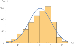
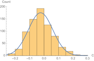
Figure 15: Distribution of the measured $\hat{x}_{1},\hat{c}$. A gaussian with matching mean and variance is superimposed. The approximate standard deviation of these distributions are $\sigma_{x1}\approx 0.99$ and $\sigma_{c}\approx 0.084$. These numbers are guiding, and play absolutely no role in the fitting procedure.

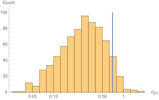
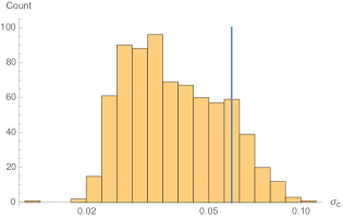
Figure 16: Distributions in logarithmic bins, of the square root of the diagonal elements of the covariance matrix for the correction parameters $x_{1},c$. These errors are to be compared with the variance of the distribution in Fig. 15. It is immediately obvious that we cannot neglect these errors when constructing the likelihood function. Indeed this looks a bit like the example Unequal errors on measurements in Sec. 2.5 — we have some intrinsic distribution which we contaminate with experimental uncertainties, so the total error is the intrinsic error and the experimental error added in quadrature. Where the two errors would be approximately equal (taken as simply the numbers quoted below Fig. 15 divided by $\sqrt{2}$) is marked by the blue line.

5.2   A statistical model of calibrated standard candles

As stated in Sec. 4.2, the corrected SN distance modulus is taken to be

$$\mu_{\text{SN}}=m_{B}^{*}-(M-\alpha x_{1}+\beta c),$$ (5.2.1)

Now we take it to be the true values that obey this relation. Writing down the likelihood for the dataset $(\hat{m}^{*}_{B1},\hat{x}_{11},\hat{c}_{1},\dots)$ is then straight forward. With a hat on observed values, we have

$$\mathcal{L}=p[(\hat{m}^{*}_{B},\hat{x}_{1},\hat{c})|\theta]=\int p[(\hat{m}^{*}_{B},\hat{x}_{1},\hat{c})|(M,x_{1},c),\theta]\ p[(M,x_{1},c)|\theta]\text{d}M\text{d}x_{1}\text{d}c$$ (5.2.2)

Here I have simply used Eq. (2.1.6) to integrate out my ignorance of the true values of the observables. I stress that $p[(M,x_{1},c)|\theta]$ is my simple model of the distribution of the correction parameters — not a (Bayesian) prior. What we need now is just the two expressions for the pdfs in this equation.

Inspired by Fig. 15 we will take the intrinsic distribution of all the parameters $M,x_{1},c$ to be independent, gaussian, and redshift independent, giving us the following pdf,

$$p[(M,x_{1},c)|\theta]=p(M|\theta)p(x_{1}|\theta)p(c|\theta),\quad\text{where:}$$ (5.2.3)

$$p(M|\theta)=(2\pi\sigma_{M_{0}}^{2})^{-1/2}\exp\left\{-\left[\left({M-M_{0}}\right)/\sigma_{M_{0}}\right]^{2}/2\right\},$$

$$p(x_{1}|\theta)=(2\pi\sigma_{x_{0}}^{2})^{-1/2}\exp\left\{-\left[\left({x_{1}-x_{0}}\right)/\sigma_{x_{0}}\right]^{2}/2\right\},$$

$$p(c|\theta)=(2\pi\sigma_{c_{0}}^{2})^{-1/2}\exp\left\{-\left[\left({c-c_{0}}\right)/\sigma_{c_{0}}\right]^{2}/2\right\}.$$

All the 6 parameters $\{M_{0},\sigma_{M_{0}},x_{0},\sigma_{x_{0}},c_{0},\sigma_{c_{0}}\}$ are fitted along with the cosmological parameters, since we have no theoretical model for what they should be. To simplify our calculations, we write this in terms of a vector $Y=\{M_{1},x_{11},c_{1},\dots M_{N},x_{1N},c_{N}\}$, the corresponding zero-points $Y_{0}$, and the covariance matrix $\Sigma_{l}=\text{diag}(\sigma_{M_{0}}^{2},\sigma_{x0}^{2},\sigma_{c0}^{2},\dots)$,

$$p[(M,x_{1},c)|\theta]=p[Y|Y_{0},\theta]={|2\pi\Sigma_{l}|}^{-1/2}\exp\left[-(Y-Y_{0})\Sigma_{l}^{-1}(Y-Y_{0})^{\text{T}}/2\right].$$ (5.2.4)

Note that this gaussian approximation is just the simplest reasonable model for these data. Introducing skewness or other such distributions may obviously lead to higher likelihoods. The main point here is that we desperately need some model, and we have no theoretical motivation for any one over another — we merely pick the simplest one.

Taking the experimental errors, statistical as well as systematic, to be described by gaussians as well, gives us the following pdf

$$p(\hat{X}|X,\theta)={|2\pi\Sigma_{\text{d}}|}^{-1/2}\exp\left[-(\hat{X}-X)\Sigma_{\text{d}}^{-1}(\hat{X}-X)^{\text{T}}/2\right],$$ (5.2.5)

where $X=\{m^{*}_{B1},x_{11},c_{1},\dots\}$, $\hat{X}$ is the observed $X$, and $\Sigma_{\text{d}}$ is the estimated experimental covariance matrix. To combine the two, we write

$$\hat{X} -X=(\hat{Z}A^{-1}-Y)A\hskip 28.45274pt\text{where}$$ (5.2.6)

$$\hat{Z} =\{\hat{m}^{*}_{B1}-\mu_{C1},\hat{x}_{11},\hat{c}_{1},\dots\},$$

$$A =\begin{pmatrix}1&0&0&\\ -\alpha&1&0&0\\ \beta&0&1&\\ &0&&\ddots\end{pmatrix},$$

where the 3-by-3 block repeats all the way down, and all other elements are zero. Hence $p[\hat{X}|X,\theta]=p[\hat{Z}|Y,\theta]$ and we get for the likelihood

$$\mathcal{L} =\int p[\hat{Z}|Y,\theta]\ p[Y|Y_{0},\theta]\text{d}Y$$ (5.2.7)

$$={|2\pi\Sigma_{\text{d}}|}^{-1/2}{|2\pi\Sigma_{l}|}^{-1/2}\int\text{d}Y$$

$$\phantom{=}\times\exp\left(-(Y-Y_{0})\Sigma_{l}^{-1}(Y-Y_{0})^{\text{T}}/2\right)$$

$$\phantom{=}\times\exp\left(-(Y-\hat{Z}A^{-1})A\Sigma_{d}^{-1}A^{\text{T}}(Y-\hat{Z}A^{-1})^{\text{T}}/2\right)$$

$$={|2\pi(\Sigma_{\text{d}}+A^{\text{T}}\Sigma_{l}A)|}^{-1/2}$$ (5.2.8)

$$\phantom{=}\times\exp\left[-(\hat{Z}-Y_{0}A)(\Sigma_{\text{d}}+A^{\text{T}}\Sigma_{l}A)^{-1}(\hat{Z}-Y_{0}A)^{\text{T}}/2\right].$$

The gaussian form of the integrand makes this integral very simple. Remember that this likelihood reflects not just our calibration of the SNe, but also the modelling of the correction parameters. From this likelihood we will find the MLE and derive confidence limits on both cosmological quantities, $\Omega_{m},\Omega_{\Lambda}$, but are also able to place constraints on the absolute magnitude scatter, the correction coefficients and the distributions of correction parameters. All these tell us about how good our model is and how well our candles are calibrated — how standard they really are.

5.3   Results of the main fit

In this section I will present the main result of the work — the MLE and confidence regions of our fit to the latest, greatest catalogue of SNe to date. Tab. 1 presents the best fits under specific constraints. The parameters are described in the previous section. In particular we see that the calibration brings the intrinsic (or at least unaccounted-for) variation to $0.108$ mag. We also get out the variances of the correction parameter distribution, which are relatively independent of the other parameters. Compared to the numbers quoted in Fig. 15 we see that the effect of experimental uncertainties is most pronounced in the colour correction, $c$, which might have been anticipated from Fig. 16.

Table 1: MLE under specific constraints, marked in boldface. $\Delta\chi^{2}$ here is short for $-2\log\mathcal{L}/\mathcal{L}_{\text{max}}$. ($-2\log\mathcal{L}_{\text{max}}=-214.97$)

Constraint $\Delta\chi^{2}$ $\Omega_{\text{m}}$ $\Omega_{\Lambda}$ $\alpha$ $x_{0}$ $\sigma_{x_{0}}$ $\beta$ $c_{0}$ $\sigma_{c_{0}}$ $M_{0}$ $\sigma_{M_{0}}$ None (best fit) $\mathbf{0}$ 0.341 0.569 0.134 0.038 0.932 3.059 -0.016 0.071 -19.052 0.108 Flat geometry 0.147 0.376 $\mathbf{0.624}$ 0.135 0.039 0.932 3.060 -0.016 0.071 -19.055 0.108 Empty universe 11.9 $\mathbf{0.000}$ $\mathbf{0.000}$ 0.133 0.034 0.932 3.051 -0.015 0.071 -19.014 0.109 Non-accelerating 11.0 0.068 $\mathbf{0.034}$ 0.132 0.033 0.931 3.045 -0.013 0.071 -19.006 0.109 Matter-less universe 10.4 $\mathbf{0.000}$ 0.094 0.134 0.036 0.932 3.059 -0.017 0.071 -19.032 0.109 Einstein-deSitter 221.97 $\mathbf{1.000}$ $\mathbf{0.000}$ 0.123 0.014 0.927 3.039 0.009 0.072 -18.839 0.125

In the spirit of cosmology, Fig. 17 presents the $1,2,$ and $3\sigma$ contours of the $\Omega_{m},\Omega_{\Lambda}$ profile likelihood and the $1$ and $2\sigma$ contours of the full likelihood, projected to the $\Omega_{m},\Omega_{\Lambda}$-plane (see Fig. 5 for how the two differ).

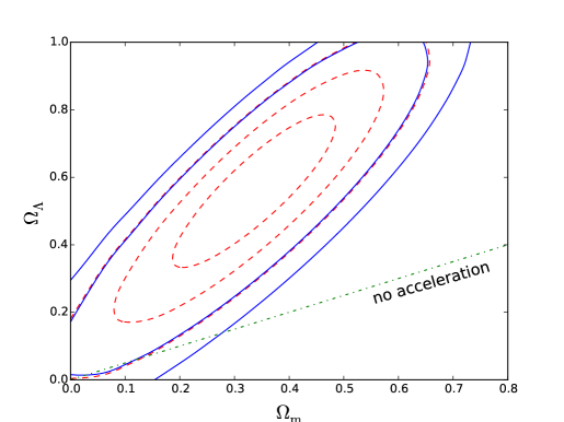
Figure 17: Contour plot of the profile likelihood in the $\Omega_{\text{m}},\Omega_{\Lambda}$ plane. 1, 2 and 3$\sigma$ contours, regarding all other parameters as nuisance parameters, are shown as red dashed lines. Blue lines mark the $1$ and $2\sigma$ 10D contours projected on to the plane (see Fig. 5 — the 2D contours describe the confidence in only $a_{\omega}$, while the 10D are the joint contour of $a_{\bot}$ and $a_{\omega}$, but only shown in $a_{\omega}$ space because of the dimensional limitations of paper).

From this figure, and the tabulated numbers, we see in particular that the non-accelerating universe is excluded at about $3\sigma$ — not overwhelming evidence. The Hubble plot we find is presented in Figs. 18 and 19.

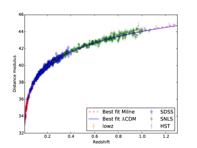
Figure 18: Comparison of data and model. The measured distance magnitudes, $\hat{\mu_{\text{SN}}}=\hat{m}^{*}_{B}-M_{0}+\alpha\hat{x}_{1}-\beta\hat{c}$ with different markers depending on the survey. The expected value in two cosmological models are also plotted. $\Lambda$CDM is the best fit accelerating universe, and Milne is an empty universe expanding with constant velocity. The error bars are the square root of the diagonal elements of $\Sigma_{l}+A^{\text{T}-1}\Sigma_{\text{d}}A^{-1}$, and include both experimental uncertainties and intrinsic dispersion. These error bars are therefore mildly correlated.

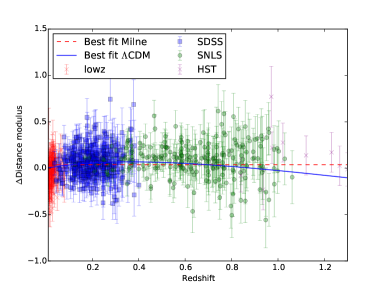
Figure 19: As Fig. 18, but with the Milne model subtracted. The Milne model plotted has had its Hubble constant corrected by changing the zero point slightly to correct for the change in $M_{0}$ — see the discussion following Eq. (4.3).

Now we want to assess how good the fit is. We simply put in gaussians as our model before, now we want to see how well this actually describes the data, along with a determination of how well the statistical approximations we do are — this is not a linear model, yet we use Wilks’ theorem to find confidence regions. In Fig. 20 are the pulls, defined as the residual, normalised to the combined expected error,

$$\text{pull}=(\hat{Z}-Y_{0}A)U^{-1},$$ (5.3.1)

where $U$ is the upper triangular Cholesky factor of the estimated covariance matrix, ie. $U^{T}U=\Sigma_{\text{d}}+A^{\text{T}}\Sigma_{l}A$. We see from the figure that while it is not a perfect description, neither is it obviously invalid. Performing a series of goodness-of-fit tests of the pull distribution to a normal distribution, we get the p-values in Tab. 2. All four tests here are looking at the cumulative distribution function in different ways. Looking at more targeted tests may give radically different answers. In particular the skewness (the third moment) is off, which might have been anticipated already from the distribution of $x_{1}$.

Figure 20: Pull distribution of the best fit model. Pulls are defined as described in Eq. (5.3.1). According to our very simple model, everything should be gaussian. Therefore we superimpose a normalised gaussian with the expected Poisson noise ($1/\sqrt{N}$).

Table 2: p-values from testing the hypothesis that the pull distribution follows a normal distribution, $\mathcal{N}(0,1)$.

Test	statistic	p-value
Anderson-Darling	2.528	0.0479
Cramér-von Mises	0.454	0.0522
Kolmogorov-Smirnov	0.0244	0.1389
Kuiper	0.0329	0.1231

We also perform a simple MC test to check that the confidence levels we set by Wilks’ theorem are good. To do so, we simulate $10^{4}$ datasets, assuming the model to be correct and taking the best fit parameters of the actual data as the model. We keep the z-values, but draw new $M,x_{1},c$ values from the predicted distributions. For every one of these datasets we find the best fit parameters, and in particular the maximum likelihood. Wilks’ theorem now states that the distribution of the quantity $-2\log\mathcal{L}_{\text{true}}/\mathcal{L}_{\text{max}}$ is a $\chi^{2}$ with $10$ degrees of freedom, where $\mathcal{L}_{\text{true}}$ is the likelihood of the true parameters. The distribution from MC and the analytic curve are plotted in Fig. 21. We see that Wilks’ theorem holds true to very high precision, and so we can indeed trust the confidence levels set by the likelihood ratio.

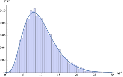
Figure 21: Distribution of the MC likelihood ratio as defined in the text. The expected $\chi^{2}$ distribution is superimposed. The excellent agreement between the two reinforces our trust in Wilks’ theorem.

5.4   Older analyses

To emphasise the strength of the present analysis, it is instructive to look at the exact differences between this and previous analyses. The previous analyses are mainly in two categories: a likelihood based one, which I argue is not a good fit, and a residual based one, which in particular is not a likelihood maximisation, and as such, what we learned in Chap. 2 no longer applies. Let us first take a look at these other methods and then return to a brief comparison with the proposed approach.

5.4.1   Residual based method

This method is the most prominent method used in analyses using the SALT method (or other methods like it) of lightcurve fitting, see eg. [78, 79, 82, 83, 84, 2]. The exact procedure varies slightly, but the main point is that one considers the quantity, which is sometimes called a $\chi^{2}$, but for pedagogical purposes I will simply call it $f$,

$$f= (m_{B}^{*}-M+\alpha x_{1}-\beta c-\mu)[\text{diag}(\sigma_{int}^{2})+C(\alpha,\beta)]^{-1}(m_{B}^{*}-M+\alpha x_{1}-\beta c-\mu)$$

$$\approx \sum\frac{\Delta\mu^{2}}{\sigma_{\mu}^{2}+\sigma_{int}^{2}}$$ (5.4.1)

where I have written out explicitly the term $\sigma_{int}$ in the covariance matrix $C$, which I write schematically as $\sigma_{\mu,i}^{2}=\sum_{ab}(\Sigma_{d,i})_{ab}r_{a}r_{b}$, where $r=(1,\alpha,-\beta)$ mixes in the relevant covariances of $x_{1},c$, and $\Sigma_{d}$ is the covariance matrix as used in the previous section. The newest version of this type of analysis tries to determine independently the $\sigma_{int}$ ([78]), while most other analyses have done something curious. First the $f$ is minimised with some plausible value of $\sigma_{int}$ inserted — typically a guess based on previous analyses. When the minimum is found, one then adjusts the $\sigma_{int}$ such that $f$ is equal to the number of degrees of freedom, say $N$. As we saw in Sec. 2.4.2 this is indeed reminiscent of fitting the unknown intrinsic error (the degree to which SNe are standard candles). But, as I stress in Sec. 2.5, not even the maximum likelihood estimate satisfies this exactly, when the errors on the datapoints are unequal. When the $f$ has now been fixed, the minimum might have moved slightly, so the procedure is iterated until convergence.

The most alarming thing is now, that confidence regions are put in place by Wilks’ theorem — even though as we just saw, this method is not derived from a likelihood, and as such using Wilks’ theorem is manifestly nonsense. However, as we will see, since the guess $f$ is an educated one, the limits one sets this way are not completely off.

5.4.2   Simple likelihood

It has been realised, that the previous method was indeed not derived from a likelihood, see [85, 86, 87, 88]. If $f$ is to be interpreted as something like $-2\log\mathcal{L}$, then we have to impose a normalisation, namely $\int\mathcal{L}\ d\text{(data)}=1$. Taking just the $m_{B}^{*}$ as the data, we see that the previous expression (5.4.1) should come from a likelihood, which takes the form

$$\mathcal{L}_{w}=\prod(2\pi[\sigma_{\mu}^{2}+\sigma_{int}^{2}])^{-1/2}\exp\left(-\frac{1}{2}\frac{\Delta\mu^{2}}{\sigma_{\mu}^{2}+\sigma_{int}^{2}}\right)$$ (5.4.2)

Now we can perform a rigorous likelihood maximisation, and construct confidence regions using Wilks’ theorem. But let’s first look closer at the likelihood we have constructed. As just stated, the way I constructed this was by regarding the integral as going over only the $m_{B}^{*}$. But there is no reason why $m_{B}^{*}$ should enjoy a privileged status compared to $x_{1},c$. It is immediate that trying to integrate over these datapoints will give infinity. So let’s see where we went wrong. To do so, we need to go back to the basics of constructing the likelihood, Eq. (5.2.2). Now put in flat distributions of $x_{1},c$, ie. instead of all gaussians, we now take

$$p(x_{1}|\theta)\propto 1$$

$$p(c|\theta)\propto 1$$ (5.4.3)

where in principle we need some compact support for these distributions to have a finite (unit) normalisation of the likelihood. Putting these distributions into Eq. (5.2.2), with the gaussian measurement errors and $p(M|\theta)$, we have, using the notation of the last section

$$\mathcal{L}_{w} \propto\frac{1}{\sqrt{|2\pi\Sigma_{d}|}}\int\exp\left[-\frac{1}{2}(\hat{X}-X)\Sigma_{d}^{-1}(\hat{X}-X)^{\text{T}}\right]\ dx_{1}\ dc$$

$$\times(2\pi\sigma_{M_{0}}^{2})^{-1/2}\exp\left\{-\left[\left({M-M_{0}}\right)/\sigma_{M_{0}}\right]^{2}/2\right\}\ dM$$ (5.4.4)

Performing first the $x_{1},c$ integrals simply mixes in the uncertainties and swaps $\hat{x}_{1},\hat{c}$ for $x_{1},c$ in $\hat{X}$. We end with, writing for simplicity just a diagonal covariance matrix,

$$\mathcal{L}_{w} \propto\int\prod_{i}\frac{1}{\sqrt{2\pi\sum_{ab}(\Sigma_{i})_{ab}r_{a}r_{b}}}\exp\left[-\frac{1}{2}\frac{[\hat{m}_{Bi}^{*}-(\mu(z_{i})+M-\alpha\hat{x}_{1i}+\beta\hat{c}_{i})]^{2}}{\sum_{ab}(\Sigma_{i})_{ab}r_{a}r_{b}}\right]$$

$$\times(2\pi\sigma_{int}^{2})^{-1/2}\exp\left\{-\left[\left({M-M_{0}}\right)/\sigma_{int}\right]^{2}/2\right\}\ dM$$ (5.4.5)

The error $\sum_{ab}(\Sigma_{i})_{ab}r_{a}r_{b}$ here is what we schematically called $\sigma_{\mu}^{2}$ before. Performing the $M$ integral now simply adds the $\sigma_{int}$ error and swaps $M$ for $M_{0}$ in the residual, which gives us the expected expression, given in Eq. (5.4.2) — up to a constant, which in principle is infinite. Putting in compact support of the $x_{1},c$ distributions complicates the integrals, but provided the limits are far away from the interesting region, the results will be almost the same. I won’t go into details about fitting these limits. The main point is that now we know exactly how this likelihood comes about, and so can say confidently that it is wrong, as we see quite clearly from Fig. 15, that we have no reason to believe the distributions of $x_{1},c$ are flat in the full range of the variables. One can of course impose narrow uniform distributions, but this will still include two extra parameters in the fit, just as the gaussian distributions do — there is no such thing as a free distribution.

5.4.3   Comparison with the present analysis

We have already seen how the naive likelihood based method compares to the present analysis. For the present purposes, let us rewrite the likelihood of Eq. (5.2.8) as

$$\mathcal{L} ={|2\pi(\Sigma_{\text{d}}+A^{\text{T}}\Sigma_{l}A)|}^{-1/2}$$ (5.4.6)

$$\phantom{=}\times\exp\left[-(\hat{Z}A^{-1}-Y_{0})(A^{T-1}\Sigma_{\text{d}}A^{-1}+\Sigma_{l})^{-1}(\hat{Z}A^{-1}-Y_{0})^{\text{T}}/2\right]$$

Taking for simplicity $\Sigma_{\text{d}}$ to be diagonal, we see that the combination of every third term in the expansion of the sum looks just like Eq. (5.4.1), notice the form of the residual here is

$$\hat{Z}A^{-1}-Y_{0}=(m_{B}^{*}-M_{0}+\alpha\hat{x}_{1}-\beta\hat{c}-\mu,\hat{x}_{1}-x_{10},\hat{c}-c_{0},\dots)$$ (5.4.7)

This means we are more or less fitting the same expressions we were before. The important thing, which has been left out of the other analyses are the terms linking residuals in $\hat{x}_{1},\hat{c}$ to those of $\hat{m}_{B}^{*}$ — the off-diagonal terms of $A^{T-1}\Sigma_{\text{d}}A^{-1}+\Sigma_{l}$. Since these analyses did not consider residuals of these terms, they obviously cannot include these corrections.

Now, that is not to say that the residual based method will give a wrong result. We just need to show it by some other means than for the MLE. In particular, since we cannot do the calculation analytically, we will have to show it by simulations. To do such a simulation though, we have to assume a distribution from which we draw the values of $x_{1}$ and $c$. To show how well the two methods should agree, I reuse the MC from Sec. 5.3 and now do both a fit with our MLE method and the residual based method. As a slight correction to the method, I use for the $\sigma_{\text{int}}$ term in the residual method the value I find from the MLE. Now, for every simulated dataset, I plot the difference in the obtained parameters in Fig. 22. This MC study is then compared to the obtained values of the actual dataset. Fitting the original dataset by the residual method, our best fit is

$$\{\Omega_{m},\Omega_{\Lambda},\alpha,\beta,M_{0}\}=\{0.200,0.591,0.134,3.08,-19.07\}$$ (5.4.8)

Figure 22: Correlations between MLE and residual method parameters, for the relevant parameters. Plotted is MLE$-$residual estimate. The dashed ellipses show approximate $1,2,3\sigma$ 2d profile contours. The blue markers show the value obtained from the real data. We see that in particular the $\Omega_{m},\Omega_{\Lambda}$ point is off. In total, there are $9945$ simulated datasets plotted.

First of all, notice that the two methods actually agree on average! This is somewhat surprising, but certainly possible. This just means that within this model the two methods agree, more or less — to the degree of spread in the figure. However, looking at the value of the real dataset, we see that it doesn’t quite agree. To put this into numbers, I first calculate the sample covariance of the MC values, $\hat{\mathcal{I}}$. Seeing the distribution of MC points as an estimate of the pdf, $\hat{\mathcal{I}}$ is the covariance of the 5d approximate gaussian distribution. We can now calculate a $\chi^{2}$ of the difference we see in the real data, as

$$\Delta\chi^{2}=\Delta\text{parameters}\cdot\hat{\mathcal{I}}^{-1}\cdot\Delta\text{parameters}\approx 22.73,$$ (5.4.9)

which for a $\chi^{2}$ distribution with 5 degrees of freedom is about $3.6\sigma$. That means, taking into consideration both fits, it is rather unlikely that they would differ by this much, if the gaussian model is correct. This fit is explicitly carried out with gaussian distributions — even for the residual method, which superficially completely disregards this information.

It is important to realise that any result obtained by the residual based method can only be validated by a MC study. This does by no means forbid it be a good estimator. What is dangerous though, is that one cannot extract from this the parameters of the underlying distributions, and so we lose the ability to eg. plot Fig. 20 in this framework. We lose the ability to assess the model of correction parameter which I emphasise, we must assume to validate the method, whether we like it or not. In particular, doing the MLE method, we have made only completely standard assumptions.

Conclusion

In this thesis I have presented in detail my knowledge of fitting cosmological parameters with supernovae. I analysed the latest large compilation of supernovae and found a result in significant contrast to the canonical result. In particular, a non-accelerating universe is only excluded at $3\sigma$ by supernovae alone. This is not to say that supernovae prefer this universe — the best fit point of this very simple model is still with a significant dark energy contribution! What we have done is to state explicitly all assumptions that are usually made. These assumptions will surely change, even in the near future. Preliminary work such as [89, 90] suggests using more and more contrived versions of the residuals based method due to selection effects, and a very recent study proposes two populations of supernovae [91]. I have in this analysis not made any such assumptions or speculations. The result I present has standard assumptions and models — only we need to state this explicitly, because we have to write down a likelihood.

This effort, I think, has two obvious products. First of all, we now have well defined confidence regions, readily compared to other analyses. We know at all times exactly what we are fitting and modelling, because we are forced to write all this down. Secondly, it gives an avenue to further exploration of the correction parameter distributions. As stated before, it is hardly believable that the distributions should be exactly gaussian, or that there is no evolution of supernovae during the evolution of the universe. The method presented here is very easily capable of dealing with this issue.

List of Figures

1. 1 Poisson distribution
2. 2 Binomial distribution
3. 3 $\chi^{2}$ distribution
4. 4 Biased coin exclusion by p-value
5. 5 Illustration of distinction between confidence region of parameters in subspaces and the full space
6. 6 $\pi$ by MC
7. 7 Error on $\pi$ by MC
8. 8 Distinction between known and unknown errors
9. 9 Distribution of obtained $\chi^{2}$s
10. 10 Straight lines curve in curved space
11. 11 Lightcurves of SN 2007af
12. 12 Plot of the original Phillips’ relation
13. 13 Distribution of SNe on the sky
14. 14 Redshift distribution of SNe
15. 15 Distribution of measured SN correction parameters
16. 16 Distribution of estimated errors on correction parameters
17. 17 Contour plot of fit to cosmological parameters
18. 18 Hubble plot
19. 19 Hubble residual plot
20. 20 Pull distribution
21. 21 Likelihood ratio distribution from MC
22. 22 MLE-residual method correlation

References

Nielsen
et al. [2015]Nielsen, J. T., Guffanti, A., andSarkar, S. 2015.
Marginal evidence for cosmic acceleration from Type Ia supernovae,
arXiv:[1506.01354].
Riess
et al. [1998]Riess, A. G.et al. 1998.
Observational evidence from supernovae for an accelerating universe
and a cosmological constant.
Astron.J.116,
1009–1038,
arXiv:[astro-ph/9805201].
Cyburt
et al. [2008]Cyburt, R. H., Fields, B. D., andOlive, K. A. 2008.
An Update on the big bang nucleosynthesis prediction for Li-7: The
problem worsens.
JCAP0811, 012,
arXiv:[0808.2818].
Hui and
Greene [2006]Hui, L.andGreene, P. B. 2006.
Correlated Fluctuations in Luminosity Distance and the (Surprising)
Importance of Peculiar Motion in Supernova Surveys.
Phys.Rev.D73, 123526,
arXiv:[astro-ph/0512159].
Kogut et al. [1993]Kogut, A., Lineweaver, C., Smoot, G. F., Bennett, C.,
Banday, A., et al. 1993.
Dipole anisotropy in the COBE DMR first year sky maps.
Astrophys.J.419, 1,
arXiv:[astro-ph/9312056].
Feindt et al. [2013]Feindt, U., Kerschhaggl, M., Kowalski, M., Aldering,
G., Antilogus, P., et al. 2013.
Measuring cosmic bulk flows with Type Ia Supernovae from the Nearby
Supernova Factory.
Astron.Astrophys.560, A90,
arXiv:[1310.4184].
Davis et al. [2011]Davis, T. M., Hui, L., Frieman, J. A., Haugbolle, T.,
Kessler, R., et al. 2011.
The effect of peculiar velocities on supernova cosmology.
Astrophys.J.741, 67,
arXiv:[1012.2912].
Weinberg [1989]Weinberg, S. 1989.
The Cosmological Constant Problem.
Rev.Mod.Phys.61, 1–23.
Velten
et al. [2014]Velten, H., vom Marttens, R., andZimdahl, W. 2014.
Aspects of the cosmological “coincidence problem”.
Eur.Phys.J.C74, 11, 3160,
arXiv:[1410.2509].
Koksma and
Prokopec [2011]Koksma, J. F.andProkopec, T. 2011.
The Cosmological Constant and Lorentz Invariance of the Vacuum
State, arXiv:[1105.6296].
Starobinsky [1980]Starobinsky, A. A. 1980.
A New Type of Isotropic Cosmological Models Without Singularity.
Phys.Lett.B91, 99–102.
Bertotti
et al. [2003]Bertotti, B., Iess, L., andTortora, P. 2003.
A test of general relativity using radio links with the Cassini
spacecraft.
Nature425, 374.
Buchert
et al. [2006]Buchert, T., Larena, J., andAlimi, J.-M. 2006.
Correspondence between kinematical backreaction and scalar field
cosmologies: The ‘Morphon field’.
Class.Quant.Grav.23, 6379–6408,
arXiv:[gr-qc/0606020].
Garcia-Bellido
and Haugboelle [2008]Garcia-Bellido, J.andHaugboelle, T. 2008.
Looking the void in the eyes - the kSZ effect in LTB models.
JCAP0809, 016,
arXiv:[0807.1326].
Bull
et al. [2012]Bull, P., Clifton, T., andFerreira, P. G. 2012.
The kSZ effect as a test of general radial inhomogeneity in LTB
cosmology.
Phys.Rev.D85, 024002,
arXiv:[1108.2222].
Celerier [2012]Celerier, M.-N. 2012.
Some clarifications about Lemaître-Tolman models of the Universe
used to deal with the dark energy problem.
Astron.Astrophys.543, A71,
arXiv:[1108.1373].
Krasinski et al. [2010]Krasinski, A., Hellaby, C., Bolejko, K., andCelerier, M.-N. 2010.
Imitating accelerated expansion of the Universe by matter
inhomogeneities: Corrections of some misunderstandings.
Gen.Rel.Grav.42, 2453–2475,
arXiv:[0903.4070].
Bolejko and
Sussman [2011]Bolejko, K.andSussman, R. A. 2011.
Cosmic spherical void via coarse-graining and averaging
non-spherical structures.
Phys.Lett.B697, 265–270,
arXiv:[1008.3420].
Szekeres [1975]Szekeres, P. 1975.
A Class of Inhomogeneous Cosmological Models.
Commun.Math.Phys.41, 55.
Bolejko and
Celerier [2010]Bolejko, K.andCelerier, M.-N. 2010.
Szekeres Swiss-Cheese model and supernova observations.
Phys.Rev.D82, 103510,
arXiv:[1005.2584].
Biswas and
Notari [2008]Biswas, T.andNotari, A. 2008.
Swiss-Cheese Inhomogeneous Cosmology and the Dark Energy Problem.
JCAP0806, 021,
arXiv:[astro-ph/0702555].
Kashlinsky et al. [2009]Kashlinsky, A., Atrio-Barandela, F., Kocevski, D., andEbeling, H. 2009.
A measurement of large-scale peculiar velocities of clusters of
galaxies: results and cosmological implications.
Astrophys.J.686, L49–L52,
arXiv:[0809.3734].
Watkins
et al. [2009]Watkins, R., Feldman, H. A., andHudson, M. J. 2009.
Consistently Large Cosmic Flows on Scales of 100 Mpc/h: a Challenge
for the Standard LCDM Cosmology.
Mon.Not.Roy.Astron.Soc.392, 743–756,
arXiv:[0809.4041].
Foley et al. [2013]Foley, R. J., Challis, P., Chornock, R., Ganeshalingam,
M., Li, W., et al. 2013.
Type Iax Supernovae: A New Class of Stellar Explosion.
Astrophys.J.767, 57,
arXiv:[1212.2209].
Clocchiatti [2011]Clocchiatti, A. 2011.
Type Ia Supernovae and the discovery of the Cosmic Acceleration,
arXiv:[1112.0706].
Chandrasekhar [1931]Chandrasekhar, S. 1931.
The Maximum Mass of Ideal White Dwarfs.
Astrophysical
Journal74, 81.
Dilday et al. [2012]Dilday, B., Howell, D., Cenko, S., Silverman, J., Nugent, P., et al. 2012.
PTF11kx: A Type-Ia Supernova with a Symbiotic Nova Progenitor.
Science337, 942, arXiv:[1207.1306].
Mazzali et al. [2007]Mazzali, P. A., Ropke, F. K., Benetti, S., andHillebrandt, W. 2007.
A Common Explosion Mechanism for Type Ia Supernovae.
Science315, 825,
arXiv:[astro-ph/0702351].
Karpenka [2015]Karpenka, N. 2015.
The supernova cosmology cookbook: Bayesian numerical recipes,
arXiv:[1503.03844].
Johnson and
Morgan [1953]Johnson, H.andMorgan, W. 1953.
Fundamental stellar photometry for standards of spectral type on the
revised system of the Yerkes spectral atlas.
Astrophys.J.117, 313.
Phillips [1993]Phillips, M. 1993.
The absolute magnitudes of Type IA supernovae.
Astrophys.J.413, L105–L108.
Tripp [1998]Tripp, R. 1998.
A Two-parameter luminosity correction for type Ia supernovae.
Astron.Astrophys.331, 815–820.
Kelly et al. [2010]Kelly, P. L., Hicken, M., Burke, D. L., Mandel, K. S.,
andKirshner, R. P. 2010.
Hubble Residuals of Nearby Type Ia Supernovae Are Correlated with
Host Galaxy Masses.
Astrophys.J.715, 743–756,
arXiv:[0912.0929].
Hayden et al. [2013]Hayden, B. T., Gupta, R. R., Garnavich, P. M., Mannucci,
F., Nichol, R. C., et al. 2013.
The Fundamental Metallicity Relation Reduces Type Ia SN Hubble
Residuals More Than Host Mass Alone.
Astrophys.J.764, 191,
arXiv:[1212.4848].
Riess
et al. [1996]Riess, A. G., Press, W. H., andKirshner, R. P. 1996.
A Precise distance indicator: Type Ia supernova multicolor light
curve shapes.
Astrophys.J.473, 88,
arXiv:[astro-ph/9604143].
Jha
et al. [2007]Jha, S., Riess, A. G., andKirshner, R. P. 2007.
Improved Distances to Type Ia Supernovae with Multicolor Light Curve
Shapes: MLCS2k2.
Astrophys.J.659, 122–148,
arXiv:[astro-ph/0612666].
Oke and
Sandage [1968]Oke, J. B.andSandage, A. 1968.
Energy Distributions, K Corrections, and the Stebbins-Whitford
Effect for Giant Elliptical Galaxies.
Astrophysical
Journal154, 21.
Schneider
et al. [2006]Schneider, P., Kochanek, C., andWambsganss, J. 2006.
Gravitational Lensing: Strong, Weak and Micro.
Springer-Verlag Berlin Heidelberg.
Kantowski
et al. [1995]Kantowski, R., Vaughan, T., andBranch, D. 1995.
The Effects of inhomogeneities on evaluating the deceleration
parameter q(0).
Astrophys.J.447, 35–42,
arXiv:[astro-ph/9511108].
Frieman [1996]Frieman, J. A. 1996.
Weak lensing and the measurement of q(0) from type Ia supernovae.
Comments Astrophys.18, 323,
arXiv:[astro-ph/9608068].
Gunnarsson et al. [2006]Gunnarsson, C., Dahlen, T., Goobar, A., Jonsson, J.,
andMortsell, E. 2006.
Corrections for gravitational lensing of supernovae: Better than
average?
Astrophys.J.640, 417–427,
arXiv:[astro-ph/0506764].
Jonsson et al. [2010]Jonsson, J., Sullivan, M., Hook, I., Basa, S., Carlberg, R., et al. 2010.
Constraining dark matter halo properties using lensed SNLS
supernovae.
Mon.Not.Roy.Astron.Soc.405, 535,
arXiv:[1002.1374].
Holz and
Linder [2005]Holz, D. E.andLinder, E. V. 2005.
Safety in numbers: Gravitational lensing degradation of the
luminosity distance-redshift relation.
Astrophys.J.631, 678–688,
arXiv:[astro-ph/0412173].
Betoule
et al. [2014]Betoule, M.et al. 2014.
Improved cosmological constraints from a joint analysis of the
SDSS-II and SNLS supernova samples.
Astron.Astrophys.568, A22,
arXiv:[1401.4064].
Conley
et al. [2011]Conley, A.et al. 2011.
Supernova Constraints and Systematic Uncertainties from the First 3
Years of the Supernova Legacy Survey.
Astrophys.J.Suppl.192, 1,
arXiv:[1104.1443].
Lyons [2013]Lyons, L. 2013.
Discovering the Significance of 5 sigma,
arXiv:[1310.1284].
Kowalski
et al. [2008]Kowalski, M.et al. 2008.
Improved Cosmological Constraints from New, Old and Combined
Supernova Datasets.
Astrophys.J.686, 749–778,
arXiv:[0804.4142].
Amanullah et al. [2010]Amanullah, R., Lidman, C., Rubin, D., Aldering, G.,
Astier, P., et al. 2010.
Spectra and Light Curves of Six Type Ia Supernovae at 0.511 z
1.12 and the Union2 Compilation.
Astrophys.J.716, 712–738,
arXiv:[1004.1711].
Wei
et al. [2015]Wei, J.-J., Wu, X.-F., Melia, F., andMaier,
R. S. 2015.
A Comparative Analysis of the Supernova Legacy Survey Sample with
CDM and the Universe.
Astron.J.149, 102,
arXiv:[1501.02838].
Marriner
et al. [2011]Marriner, J., Bernstein, J. P., Kessler, R., Lampeitl,
H., Miquel, R., Mosher, J., Nichol, R. C., Sako, M.,
andSmith, M. 2011.
A More General Model for the Intrinsic Scatter in Type Ia Supernova
Distance Moduli.
Astrophys.
J.740, 72,
arXiv:[1107.4631].
Kessler
et al. [2013]Kessler, R.et al. 2013.
Testing Models of Intrinsic Brightness Variations in Type Ia
Supernovae, and their Impact on Measuring Cosmological Parameters.
Astrophys.
J.764, 48,
arXiv:[1209.2482].
Milne
et al. [2015]Milne, P. A., Foley, R. J., Brown, P. J., andNarayan, G. 2015.
The Changing Fractions of Type ia Supernova Nuv–optical Subclasses
With Redshift.
Astrophys.J.803, 1, 20,
arXiv:[1408.1706].
Figure 4: p-value, given by Eq. (2.4.34), of different outcomes from tossing a coin times for different values of as labeled in the legend. This tests the hypothesis that the coin is fair.
Figure 5: Illustration of confidence regions for two parameters with . The dashed contour shows the confidence region of both parameters, while the dotted lines are the boundaries of the confidence interval, taking to be a nuisance parameter. As shown, these dotted lines mark the extreme for which any gives . The number is the solution to the equation . For higher dimensions, one could also give the boundaries of the joint contour in lower dimensions — here the boundary would be at instead of . It is important though, to remember the difference in meaning. The bigger one also contains information on the other parameter, while the small one take all but as nuisance parameters.
Figure 6: Example of MC integration. Each point is drawn at random. In this case, . This means the confidence interval for the integral is approximately , compared to the true value, , we see that this is indeed a reasonable estimate.
Figure 7: Errors from the computation of by MC integration. We see that all the errors are of expected magnitude (notice that it is plotted on log-log axes). For every , I perform MC simulations, simply to show the intrinsic variability in the estimate.