Collider Phenomenology of the 3-3-1 Model

Abstract

We study collider phenomenology of the so-called 331 model with $SU(3)_{C}\otimes SU(3)_{L}\otimes U(1)_{X}$ gauge structure at the large hadron collider, including single and double Higgs boson productions, Higgs boson rare decay, $Z^{\prime}$ boson production, new charged gauge boson pair production, and heavy quark pair production. We discuss all the possible collider signatures of new particle productions. Four benchmark 331 models, $\beta=\pm\sqrt{3}$ and $\beta=\pm 1/\sqrt{3}$, are studied in this work.

1 Introduction

The 331 model is a simple extension of the SM based on the gauge group $SU(3)_{C}\times SU(3)_{L}\times U(1)_{X}$ Frampton (1992); Pisano and Pleitez (1992). There are different versions Dias and Pleitez (2004); Dias et al. (2003); Diaz et al. (2005); Dias et al. (2005a); Dias (2005); Dias et al. (2005b, c, 2011); Ochoa and Martinez (2005) of this model which can be characterized by a parameter called $\beta$. Models with different $\beta$ have new particles with different electric charges. But in general, they all have the same features. i) Unlike the SM that anomaly cancellation is fulfilled within each generation, the gauger anomaly is cancelled in the 331 model when considering all the generations. In particular, the number of triplets must be equal to the number of anti-triplets in fermion sector, due to the nontrivial $SU(3)$ gauge structure. The number of generations $N$ must be a multiple of three. On the other hand, in order to ensure QCD an asymptotic free theory, $N$ has to be smaller than six. So the number of generations $N$ is equal to three. That explains why the SM has three generations. ii) One of the three quark generations is different from the other two, making sure that the anomaly is free, which leads to tree-level Flavour Changing Neutral Current (FCNC) through a new neutral gauge boson $Z^{\prime}$ or the mixing of $Z$ and $Z^{\prime}$. And if we choose the third generation of quark as a different one, the heavy top quark mass may be explained. iii) Peccei-Quinn (PQ) symmetry Peccei and Quinn (1977) which can solve the strong CP problem is a natural result of gauge invariance in the 331 model Dias and Pleitez (2004); Dias et al. (2003). Thus PQ symmetry does not suffer from quantum corrections, which means it is not a classical symmetry but a quantum-level one. iiii) With the extension of gauge group, particles in the 331 model are richer than the SM. For instance, there will be three more gauge bosons, three more heavy quarks or leptons and six more Higgs scalars, which gives rise to very rich phenomenology at the LHC.

The 331 model has already been studied in many aspects. For the collider physics, the research of the SM Higgs boson Ninh and Long (2005), charged Higgs boson Okada et al. (2016a); Martinez and Ochoa (2012); Montalvo et al. (2012); Alves et al. (2011); Cieza Montalvo et al. (2008a, b, c); Soa et al. (2007); Van Soa and Le Thuy (2006); Cieza Montalvo et al. (2006), $Z^{\prime}$ Salazar et al. (2015); Coutinho et al. (2013); Martinez and Ochoa (2009); Ramirez Barreto et al. (2007, 2006); Salazar et al. (2015), exotic quark do Amaral Coutinho et al. (1999); Cabarcas et al. (2008) have already been done by many people. For the neutrino physics, people have studied how to generate the small neutrino mass in different versions of the 331 model Okada et al. (2016b); Boucenna et al. (2014); Benavides et al. (2015); Boucenna et al. (2015a); Ky and Van (2005). The usual way to generate the neutrino mass is through seesaw mechanism, loop induced process or high dimensional operator. A recent review of neutrino mass mechanisms in the 331 model can be found in Pires (2014). For the fermion mass mixing, different flavor symmetries including $D_{4}$ Vien and Long (2015a); Vien (2014); Vien and Long (2013), $S_{3}$ Cárcamo Hernández et al. (2015); Vien and Long (2014a); Cárcamo Hernández et al. (2013); Dong et al. (2012), $A_{4}$ Cárcamo Hernández and Martinez (2016); Vien and Long (2015b); Dong et al. (2010), $S_{4}$ Vien et al. (2015); Dong et al. (2011), $T_{7}$ Cárcamo Hernández and Martinez (2015); Vien and Long (2014b) and $\Delta_{27}$ Vien et al. (2016); Cárcamo Hernández et al. (2016) have been introduced to explain the fermion mass mixing pattern. In the dark matter aspect, there is a residual $Z_{2}$ symmetry Mizukoshi et al. (2011) after spontaneously symmetry breaking (SSB). The lightest particle in the $Z_{2}$-odd sector will be a dark matter candidate. Researches related to this aspect can be found in Ref. de S. Pires et al. (2016); Dong et al. (2015); Cogollo et al. (2014); Dong et al. (2014, 2013). Since there will be tree-level FCNC processes through $Z^{\prime}$ or neutral scalars, it is necessary to consider the constraints from $B$, $D$ and $K$ mesons Buras and De Fazio (2016a, b); Dong and Ngan (2015); Correia and Pleitez (2015); Machado et al. (2013); Buras et al. (2014a); De Fazio (2013); Cogollo et al. (2012); Benavides et al. (2009); Promberger et al. (2007); Rodriguez and Sher (2004). Lepton flavor violation process can be generated because of introducing the third component of lepton fields Fonseca and Hirsch (2016); Machado et al. (2016); Boucenna et al. (2015b); Hue et al. (2016); Hua and Yue (2014); Van Soa et al. (2009). New contributions to the electron and neutron electric dipole moment (EDM) De Conto and Pleitez (2016a); De Conto and Pleitez (2015) and muon $g-2$ De Conto and Pleitez (2016b); Binh et al. (2015); Kelso et al. (2014a, b) through new charged scalars and charged gauge bosons have also been studied.

In this work, we consider different versions of the 331 model, namely $\beta=\pm\sqrt{3},\pm 1/\sqrt{3}$. For simplicity, we do not consider FCNC and the mixing of $Z$ and $Z^{\prime}$ since they are too small to affect the processes of interest to us. Detailed discussions of the FCNC interactions in the $331$ model can be found in Refs. Buras et al. (2014b); Rebello Teles (2013); Cabarcas et al. (2012); Carcamo Hernandez et al. (2006).

The paper is organized as follows. In Sec. 2 we introduce the $331$ model briefly. In Sec. 3, we discuss the Higgs boson phenomenology in the 331 model. We derive constraints on the parameter space of the 331 model from the single Higgs boson measurements and then discuss the Higgs rare decay, $\sigma(pp\to h\to Z\gamma)$, and di-Higgs boson production $\sigma(pp\to hh)$ at the LHC. We study the production and decay of the new particles ($Z^{\prime},~{}V,~{}Y,~{}D,~{}S,~{}T$) in this model and give the possible collider signature of those particles in Sec. 4, 5 and 6. In the last section, we will make a conclusion. In Appendix A, we list the Feynman rules of the interaction vertices in unitary gauge in the 331 model. Appendix B is used to give a detailed expression of the rotation matrix for the neutral scalars. The loop functions in the loop-induced decay width of the Higgs boson is shown in Appendix C.

2 The Model

The 331 model has been studied in details in Ref. Buras et al. (2013). In this section we briefly review the model and present the masses of new physics resonances. All the Feynman rules of the interaction vertices in unitary gauge among the new scalar sector, the new gauge bosons, the new fermions and the SM particles can be found in Appendix A. Three-point couplings of one gauge boson to two scalars ($VSS$) are listed in Table LABEL:1gauge-2scalars. Three-point couplings of two gauge bosons to one scalar ($VVS$) are listed in Table LABEL:2gauges-1scalar. Four-point couplings of two gauge bosons to two scalars ($VVSS$) are listed in Table LABEL:2gauges-2scalars. Gauge boson self-couplings are listed in Table LABEL:gauges. Gauge boson-fermion couplings are listed in Table LABEL:gauge-fermion. Scalar-fermion couplings are listed in Table LABEL:scalar-fermion.

2.1 Higgs Sector

The symmetry breaking pattern of the 331 model is

$$SU(3)_{L}\times U(1)_{X}\rightarrow SU(2)_{L}\times U(1)_{Y}\rightarrow U(1)_{Q},$$ (1)

which is realized by introducing three Higgs triplets $\rho$, $\eta$ and $\chi$

$$\rho=\left(\begin{array}[]{c}\rho^{+}\\ \rho^{0}\\ \rho^{-Q_{V}}\\ \end{array}\right)\quad\eta=\left(\begin{array}[]{c}\eta^{0}\\ \eta^{-}\\ \eta^{-Q_{Y}}\\ \end{array}\right)\quad\chi=\left(\begin{array}[]{c}\chi^{Q_{Y}}\\ \chi^{Q_{V}}\\ \chi^{0}\\ \end{array}\right),$$ (2)

where $Q_{V}$ and $Q_{Y}$ are the undetermined electric charges of the corresponding Higgs fields. The vacuum expectation values (vevs) of $\rho$, $\eta$ and $\chi$ are chosen as follows:

$$\left<\rho\right>=\frac{1}{\sqrt{2}}\left(\begin{array}[]{c}0\\ v_{1}\\ 0\\ \end{array}\right),\quad\left<\eta\right>=\frac{1}{\sqrt{2}}\left(\begin{array}[]{c}v_{2}\\ 0\\ 0\\ \end{array}\right),\quad\left<\chi\right>=\frac{1}{\sqrt{2}}\left(\begin{array}[]{c}0\\ 0\\ v_{3}\\ \end{array}\right).$$ (3)

At the first step of the symmetry breaking, $\chi$ is introduced to break $SU(3)_{L}\times U(1)_{X}$ to $SU(2)_{L}\times U(1)_{Y}$ at a very large scale $v_{3}$, typically at $\,{\rm TeV}$ scale. At the second step, we use $\rho$ and $\eta$ to break $SU(2)_{L}\times U(1)_{Y}$ down to the residual $U(1)_{Q}$ electromagnetic symmetry at about the weak scale, i.e. $v_{1}\sim v_{2}\sim m_{W}$. Thus, we have $v_{3}$ $\gg$ $v_{1,2}$, named as the “decoupling limit”. The symmetry breaking pattern is shown in Fig. 1.

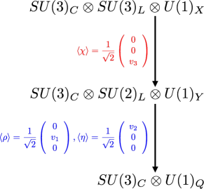
Figure 1: The symmetry breaking pattern of the 331 model.

The hypercharge generator is obtained by a linear combination of $X$ and $T^{8}$,

$$Y=\beta T^{8}+X,$$ (4)

where $T^{8}$ is diagonal generator of $SU(3)_{L}$ and $X$ is the generator of $U(1)_{X}$. That leads to the electric charge generator as

$$Q=T^{3}+\beta T^{8}+X.$$ (5)

The $X$ quantum numbers of the three Higgs triplets can be fixed by the electric charge generator as follows:

$$X_{\rho}=\frac{1}{2}-\frac{\beta}{2\sqrt{3}},\quad X_{\eta}=-\frac{1}{2}-\frac{\beta}{2\sqrt{3}},\quad X_{\chi}=\frac{\beta}{\sqrt{3}},$$ (6)

which give rise to the $Q_{Y}$ and $Q_{V}$ of those scalars in Eq. (2) as follows:

$$Q_{Y}=\frac{\sqrt{3}}{2}\beta+\frac{1}{2},\quad Q_{V}=\frac{\sqrt{3}}{2}\beta-\frac{1}{2}.$$ (7)

The Lagrangian of the Higgs sector are

$${\cal L}_{Higgs}=(D_{\mu}\rho)^{\dagger}(D^{\mu}\rho)+(D_{\mu}\eta)^{\dagger}(D^{\mu}\eta)+(D_{\mu}\chi)^{\dagger}(D^{\mu}\chi)-V_{Higgs},$$ (8)

with the Higgs potential

$$V_{Higgs} = \mu_{1}^{2}(\rho^{\dagger}\rho)+\mu_{2}^{2}(\eta^{\dagger}\eta)+\mu_{3}^{2}(\chi^{\dagger}\chi)+\lambda_{1}(\rho^{\dagger}\rho)^{2}+\lambda_{2}(\eta^{\dagger}\eta)^{2}+\lambda_{3}(\chi^{\dagger}\chi)^{2}$$ (9)

$$+ \lambda_{12}(\rho^{\dagger}\rho)(\eta^{\dagger}\eta)+\lambda_{13}(\rho^{\dagger}\rho)(\chi^{\dagger}\chi)+\lambda_{23}(\eta^{\dagger}\eta)(\chi^{\dagger}\chi)$$

$$+ \lambda^{\prime}_{12}(\rho^{\dagger}\eta)(\eta^{\dagger}\rho)+\lambda^{\prime}_{13}(\rho^{\dagger}\chi)(\chi^{\dagger}\rho)+\lambda^{\prime}_{23}(\eta^{\dagger}\chi)(\chi^{\dagger}\eta)$$

$$+ \sqrt{2}f(\epsilon_{ijk}\rho^{i}\eta^{j}\chi^{k}+h.c.),$$

where the $\lambda^{(\prime)}_{i(j)}$’s denote the dimensionless parameter while the $\mu_{i}$ and $f$ are mass-dimensional parameters. For simplicity, we assume that $f$ is proportional to $v_{3}$, $f=kv_{3}$ with $k\sim O(1)$, such that the model has no other scale.

2.1.1 Neutral scalars

The neutral scalar fields can be written in terms of their real and imaginary components explicitly

$$\rho^{0}={1\over\sqrt{2}}(\xi_{\rho}+i\zeta_{\rho}),\quad\eta^{0}={1\over\sqrt{2}}(\xi_{\eta}+i\zeta_{\eta}),\quad\chi^{0}={1\over\sqrt{2}}(\xi_{\chi}+i\zeta_{\chi}).$$ (10)

When the real components of those scalars develop the vacuum expectation values, the Higgs potential gives rise to a mass matrix of those read components as following

$$M_{H}^{2}=\left(\begin{array}[]{ccc}2\lambda_{1}v_{1}^{2}+\frac{fv_{2}v_{3}}{v_{1}}&-fv_{3}+v_{1}v_{2}\lambda_{12}&-fv_{2}+v_{1}v_{3}\lambda_{13}\\ -fv_{3}+v_{1}v_{2}\lambda_{12}&2\lambda_{2}v_{2}^{2}+\frac{fv_{1}v_{3}}{v_{2}}&-fv_{1}+v_{2}v_{3}\lambda_{23}\\ -fv_{2}+v_{1}v_{3}\lambda_{13}&-fv_{1}+v_{2}v_{3}\lambda_{23}&2\lambda_{3}v_{3}^{2}+\frac{fv_{1}v_{2}}{v_{3}}\\ \end{array}\right).$$ (11)

Three CP-even scalars emerge after the symmetry breaking as the eigenstates of the mass matrix in Eq. (11) and one scalar is identified as the SM Higgs boson ($h$). The other two scalars are named as $H_{1}$ and $H_{2}$. Even though the masses of the three scalars can be solved analytically by diagonalizing the mass matrix, the expressions are too complicated to show here. For simplicity, we expand the CP-even scalar masses in the decoupling limit, $v_{3}\gg v_{1,2}$, which yields three mass eigenvalues at the lowest order as following

$$m_{h}^{2}=\frac{2\left(\lambda_{1}v_{1}^{4}+\lambda_{12}v_{1}^{2}v_{2}^{2}+\lambda_{2}v_{2}^{4}\right)}{v^{2}},\quad M_{H_{2}}^{2}=\frac{v^{2}}{v_{1}v_{2}}fv_{3},\quad M_{H_{3}}^{2}=2\lambda_{3}v_{3}^{2},$$ (12)

where $v^{2}\equiv v_{1}^{2}+v_{2}^{2}$. As to be shown soon, we require

$$v=\sqrt{v_{1}^{2}+v_{2}^{2}}=246~{}{\rm GeV}.$$ (13)

in order to obtain the correct mass of the $W$-boson. The three neutral scalars $h$, $H_{2}$ and $H_{3}$ are related with the weak eigenstates by a rotation matrix $U$

$$\left(\begin{array}[]{c}h\\ H_{2}\\ H_{3}\\ \end{array}\right)=\left(\begin{array}[]{c c c}U_{11}&U_{12}&U_{13}\\ U_{21}&U_{22}&U_{23}\\ U_{31}&U_{32}&U_{33}\\ \end{array}\right)^{\dagger}\left(\begin{array}[]{c}\xi_{\rho}\\ \xi_{\eta}\\ \xi_{\chi}\\ \end{array}\right).$$ (14)

The rotation matrix can also be analytically solved in terms of those three eigenvalues. In this work we focus on the three matrix element in the first column and explore the phenomenology of the Higgs boson. One can expand the matrix elements in the decoupling limit $v_{3}\gg v_{1,2}$. To the lowest order, the results are

$$U_{11}=c_{12}+\frac{g_{11}(v)}{v_{3}^{2}},\quad U_{21}=s_{12}+\frac{g_{21}(v)}{v_{3}^{2}},\quad U_{31}=\frac{g_{31}(v)}{v_{3}},$$ (15)

where we have defined

$$s_{12}=\frac{v_{2}}{v},\quad c_{12}=\frac{v_{1}}{v}$$ (16)

and $g_{i1}(v)$ are functions independent of $v_{3}$. The detailed expression of $g_{i1}(v_{1})$ is given in Appendix B.

For the imaginary part of the neutral scalars, the mass mixing matrix is

$$M_{H^{\prime}}^{2}=\left(\begin{array}[]{ccc}v_{2}v_{3}/v_{1}&v_{3}&v_{2}\\ v_{3}&v_{1}v_{3}/v_{2}&v_{1}\\ v_{2}&v_{1}&v_{1}v_{2}/v_{3}\\ \end{array}\right)f.$$ (17)

The three mass eigenvalues are

$$M_{H_{0}}^{2}=\frac{f\left(v_{1}^{2}v_{2}^{2}+v_{3}^{2}v_{2}^{2}+v_{1}^{2}v_{3}^{2}\right)}{v_{1}v_{2}v_{3}},\quad M_{G_{Z}}^{2}=0,\quad M_{G_{Z^{\prime}}}^{2}=0.$$ (18)

Here, $H_{0}$ refers to the CP-odd Higgs boson, while $G_{Z}$ and $G_{Z^{\prime}}$ represent the goldstone bosons eaten by gauge bosons $Z$ and $Z^{\prime}$ respectively. The mass eigenstates are linked with the weak eigenstates by the following rotation matrix $O$

$$\left(\begin{array}[]{c}H_{0}\\ G_{Z}\\ G_{Z^{\prime}}\\ \end{array}\right)=\left(\begin{array}[]{ccc}O_{11}&O_{12}&O_{13}\\ O_{21}&O_{22}&O_{23}\\ O_{31}&O_{32}&O_{33}\\ \end{array}\right)^{\dagger}\left(\begin{array}[]{c}\zeta_{\rho}\\ \zeta_{\eta}\\ \zeta_{\chi}\\ \end{array}\right).$$ (19)

See Appendix B for detailed expressions of $O_{ij}$’s. In the decoupling limit, we obtain

$$O_{11}=O_{22}=s_{12},\quad O_{21}=-O_{12}=c_{12},\quad O_{i3}=O_{3i}=0,\quad O_{33}=1.$$ (20)

2.1.2 Charged scalars

In addtion to the neutral scalars mentioned above, there are three kinds of charged scalars whose electric charges are $\pm 1$, $\pm Q_{Y}$ and $\pm Q_{V}$. The mass mixing matrix of charge $\pm 1$ is

$$M_{\pm 1}^{2}=\left(\begin{array}[]{ccc}\dfrac{1}{2}\lambda^{\prime}_{12}v_{2}^{2}+\dfrac{fv_{3}v_{2}}{v_{1}}&{}{}\hfil&-fv_{3}-\dfrac{1}{2}v_{1}v_{2}\lambda^{\prime}_{12}\\ -fv_{3}-\dfrac{1}{2}v_{1}v_{2}\lambda^{\prime}_{12}&{}{}\hfil&\dfrac{1}{2}\lambda^{\prime}_{12}v_{1}^{2}+\dfrac{fv_{3}v_{1}}{v_{2}}\\ \end{array}\right),$$ (21)

with two mass eigenvalues

$$M_{G^{\pm}}^{2}=0,\quad M_{H^{\pm}}^{2}=\frac{2fv_{3}+\lambda^{\prime}_{12}v_{1}v_{2}}{2v_{1}v_{2}}v^{2}.$$ (22)

The $H^{\pm}$ scalars are the physical states with electric charge $\pm 1$, and $G^{\pm}$ are the goldstone bosons eaten by $W^{\pm}$. The rotation matrix from weak eigenstates to mass eigenstates is

$$\left(\begin{array}[]{c}H^{\pm}\\ G^{\pm}\\ \end{array}\right)=\left(\begin{array}[]{cc}c_{12}&-s_{12}\\ s_{12}&c_{12}\\ \end{array}\right)\left(\begin{array}[]{c}\eta^{\pm}\\ \rho^{\pm}\\ \end{array}\right),$$ (23)

The mass mixing matrix of charge $\pm Q_{Y}$ is

$$M_{\pm Q_{Y}}^{2}=\left(\begin{array}[]{ccc}\dfrac{1}{2}\lambda^{\prime}_{23}v_{3}^{2}+\dfrac{fv_{1}v_{3}}{v_{2}}&{}{}\hfil&-fv_{1}-\dfrac{1}{2}v_{2}v_{3}\lambda^{\prime}_{23}\\ -fv_{1}-\dfrac{1}{2}v_{2}v_{3}\lambda^{\prime}_{23}&{}{}\hfil&\dfrac{1}{2}\lambda^{\prime}_{23}v_{2}^{2}+\dfrac{fv_{1}v_{2}}{v_{3}}\\ \end{array}\right),$$ (24)

with the mass eigenvalues

$$M_{G^{\pm Q_{Y}}}^{2}=0,\quad M_{H^{\pm Q_{Y}}}^{2}=\frac{2fv_{1}+\lambda^{\prime}_{23}v_{2}v_{3}}{2v_{2}v_{3}}(v_{2}^{2}+v_{3}^{2}).$$ (25)

The $H^{\pm Q_{Y}}$ scalars stand for the physical states with electric charge $\pm Q_{Y}$ while $G^{\pm Q_{Y}}$ are the goldstone bosons eaten by new gauge bosons $Y^{\pm Q_{Y}}$’s. The rotation matrix from weak eigenstates to mass eigenstates is

$$\left(\begin{array}[]{c}H^{\pm Q_{Y}}\\ G^{\pm Q_{Y}}\\ \end{array}\right)=\left(\begin{array}[]{cc}c_{23}&-s_{23}\\ s_{23}&c_{23}\\ \end{array}\right)\left(\begin{array}[]{c}\chi^{\pm Q_{Y}}\\ \eta^{\pm Q_{Y}}\\ \end{array}\right),$$ (26)

where we define

$$s_{23}=\frac{v_{3}}{\sqrt{v_{2}^{2}+v_{3}^{2}}},\quad c_{23}=\frac{v_{2}}{\sqrt{v_{2}^{2}+v_{3}^{2}}}.$$ (27)

As for the charged scalars with electric charge $\pm Q_{V}$, the mass mixing matrix is

$$M_{\pm Q_{V}}^{2}=\left(\begin{array}[]{ccc}\dfrac{1}{2}\lambda^{\prime}_{13}v_{3}^{2}+\dfrac{fv_{2}v_{3}}{v_{1}}&{}{}\hfil&-fv_{2}-\dfrac{1}{2}v_{1}v_{3}\lambda^{\prime}_{13}\\ -fv_{2}-\dfrac{1}{2}v_{1}v_{3}\lambda^{\prime}_{13}&{}{}\hfil&\dfrac{1}{2}\lambda^{\prime}_{13}v_{1}^{2}+\dfrac{fv_{2}v_{1}}{v_{3}}\\ \end{array}\right),$$ (28)

with two mass eigenvalues

$$M_{G^{\pm Q_{V}}}^{2}=0,\quad M_{H^{\pm Q_{V}}}^{2}=\frac{2fv_{2}+\lambda^{\prime}_{13}v_{1}v_{3}}{2v_{1}v_{3}}(v_{1}^{2}+v_{3}^{2}).$$ (29)

Here, $H^{\pm Q_{V}}$ represent the physical states with electric charge $\pm Q_{V}$ while $G^{\pm Q_{V}}$’s are the goldstone bosons eaten by new gauge bosons $V^{\pm Q_{V}}$’s. The rotation matrix from weak eigenstates to mass eigenstates are

$$\left(\begin{array}[]{c}H^{\pm Q_{V}}\\ G^{\pm Q_{V}}\\ \end{array}\right)=\left(\begin{array}[]{cc}c_{13}&-s_{13}\\ s_{13}&c_{13}\\ \end{array}\right)\left(\begin{array}[]{c}\chi^{\pm Q_{V}}\\ \rho^{\pm Q_{V}}\\ \end{array}\right),$$ (30)

where we define

$$s_{13}=\frac{v_{3}}{\sqrt{v_{1}^{2}+v_{3}^{2}}},\quad c_{13}=\frac{v_{1}}{\sqrt{v_{1}^{2}+v_{3}^{2}}}.$$ (31)

2.2 Gauge Sector

The Lagrangian of the gauge sector is

$${\cal L}_{Gauge}=-\frac{1}{4}F_{\mu\nu}F^{\mu\nu}-\frac{1}{4}B_{\mu\nu}B^{\mu\nu},$$ (32)

where $F_{\mu\nu}$ and $B_{\mu\nu}$ are field strength tensors of $SU(3)_{L}$ and $U(1)_{X}$

$$F_{\mu\nu}=\partial_{\mu}W^{i}_{\nu}-\partial_{\nu}W^{i}_{\mu},\quad B_{\mu\nu}=\partial_{\mu}X_{\nu}-\partial_{\nu}X_{\mu}.$$ (33)

Here, $W^{i}_{\mu}$ and $X_{\mu}$ denotes the gauge fields of $SU(3)_{L}$ and $U(1)_{X}$, respectively, where the index $i$ runs from 1 to 8.

After the spontaneous symmetry breaking (SSB), gauge bosons obtain their masses from the kinetic terms of the Higgs fields

$${\cal L}_{Higgs}^{kinetic}=(D_{\mu}\rho)^{\dagger}(D^{\mu}\rho)+(D_{\mu}\eta)^{\dagger}(D^{\mu}\eta)+(D_{\mu}\chi)^{\dagger}(D^{\mu}\chi).$$ (34)

We explicitly write out the specific terms responsible for the masses of the gauge bosons

$${\cal L}_{Gauge}^{mass} = \left<\chi\right>^{\dagger}G_{\mu}^{\dagger}G^{\mu}\left<\chi\right>+\left<\rho\right>^{\dagger}G_{\mu}^{\dagger}G^{\mu}\left<\rho\right>+\left<\eta\right>^{\dagger}G_{\mu}^{\dagger}G^{\mu}\left<\eta\right>$$ (39)

$$= (\left<\chi\right>+\left<\rho\right>+\left<\eta\right>)^{\dagger}G_{\mu}^{\dagger}G^{\mu}(\left<\chi\right>+\left<\rho\right>+\left<\eta\right>)$$

$$= \frac{1}{2}\left(\begin{array}[]{ccc}v_{2}&v_{1}&v_{3}\\ \end{array}\right)G_{\mu}^{\dagger}G^{\mu}\left(\begin{array}[]{c}v_{2}\\ v_{1}\\ v_{3}\\ \end{array}\right),$$

where

$$G_{\mu} =gW^{i}_{\mu}T^{i}+g_{X}XX_{\mu}T^{9}$$

$$= {1\over 2}\left(\begin{array}[]{ccc}g(W_{\mu}^{3}+{1\over\sqrt{3}}W_{\mu}^{8})+2g_{X}XX_{\mu}&\sqrt{2}gW_{\mu}^{+}&\sqrt{2}gY_{\mu}^{+Q_{Y}}\\ \sqrt{2}gW_{\mu}^{-}&-g(W_{\mu}^{3}-{1\over\sqrt{3}}W_{\mu}^{8})+2g_{X}X_{\mu}&\sqrt{2}gV_{\mu}^{+Q_{V}}\\ \sqrt{2}gY_{\mu}^{-Q_{Y}}&\sqrt{2}gV_{\mu}^{-Q_{V}}&-{2\over\sqrt{3}}gW_{\mu}^{8}+2g_{X}XX_{\mu}\end{array}\right).$$

In the above equation, $g$ and $g_{X}$ are coupling constants of $SU(3)_{L}$ and $U(1)_{X}$ respectively. $2T^{i}$ are eight Gell-Mann Matrices. $T^{9}$ is just the Identity matrix. $X$ is the $U(1)_{X}$ quantum number of some specific Higgs fields. We also define the mass eigenstates of the charged gauge bosons as follows

$$W^{\pm}_{\mu}=\frac{1}{\sqrt{2}}(W^{1}_{\mu}\mp iW^{2}_{\mu}),\quad Y^{\pm Q_{Y}}_{\mu}=\frac{1}{\sqrt{2}}(W^{4}_{\mu}\mp iW^{5}_{\mu}),\quad V^{\pm Q_{V}}_{\mu}=\frac{1}{\sqrt{2}}(W^{6}_{\mu}\mp iW^{7}_{\mu}).$$ (43)

Inserting Eq. (2.2) into (39) and also using the $X$ quantum numbers given in E.q (6), one can get the mass terms of gauge bosons as follows

$${\cal L}_{Gauge}^{mass} = \frac{1}{4}g^{2}v^{2}W_{\mu}^{+}W^{\mu,-}+\frac{1}{4}g^{2}(v_{2}^{2}+v_{3}^{2})Y_{\mu}^{Q_{Y}}Y^{\mu,-Q_{Y}}+\frac{1}{4}g^{2}(v_{1}^{2}+v_{3}^{2})V_{\mu}^{Q_{V}}V^{\mu,-Q_{V}}$$ (44)

$$+ ~{}\frac{1}{6}v_{3}^{2}(-gW_{\mu}^{8}+\beta g_{X}X_{\mu})^{2}+\frac{1}{8}v_{1}^{2}\left[-gW_{\mu}^{3}+\frac{1}{\sqrt{3}}gW_{\mu}^{8}+\big{(}1-\frac{\beta}{\sqrt{3}}\big{)}g_{X}X_{\mu})\right]^{2}$$

$$+ ~{}\frac{1}{8}v_{2}^{2}\left[gW_{\mu}^{3}+\frac{1}{\sqrt{3}}gW_{\mu}^{8}-(1+\frac{\beta}{\sqrt{3}})g_{X}X_{\mu})\right]^{2}.$$

The masses of the charged gauge bosons are given by

$$M^{2}_{W^{\pm}}=\frac{g^{2}}{4}v^{2},\quad M^{2}_{Y^{\pm Q_{Y}}}=\frac{g^{2}}{4}(v_{3}^{2}+v_{2}^{2}),\quad M^{2}_{V^{\pm Q_{V}}}=\frac{g^{2}}{4}(v_{3}^{2}+v_{1}^{2}),$$ (45)

where $v$ is the vacuum expectation value of $246~{}{\rm GeV}$ in the SM.

The $3\times 3$ mass mixing matrix of the neutral gauge bosons is

$$M_{NG}^{2}=\left(\begin{array}[]{ccc}A&\quad B&\quad C\\ B&\quad g^{2}v^{2}/8&\quad g^{2}\left(v_{2}^{2}-v_{1}^{2}\right)/8\sqrt{3}\\ C&\quad g^{2}\left(v_{2}^{2}-v_{1}^{2}\right)/8\sqrt{3}&\quad g^{2}\left(v^{2}+4v_{3}^{2}\right)/24\\ \end{array}\right),$$ (46)

with

$$A = \frac{1}{24}g_{x}^{2}\left[\left(\beta^{2}-2\sqrt{3}\beta+3\right)v_{1}^{2}+\left(\beta^{2}+2\sqrt{3}\beta+3\right)v_{2}^{2}+4\beta^{2}v_{3}^{2}\right],$$ (47)

$$B = \frac{1}{24}gg_{x}\left[\left(\sqrt{3}\beta-3\right)v_{1}^{2}-\left(\sqrt{3}\beta+3\right)v_{2}^{2}\right],$$ (48)

$$C = \frac{1}{24}gg_{x}\left[\left(\sqrt{3}-\beta\right)v_{1}^{2}-\left(\beta+\sqrt{3}\right)v_{2}^{2}-4\beta v_{3}^{2}\right].$$ (49)

The three eigenvalues of the above matrix can be solved analytically. One zero eigenvalue corresponds to the massless photon, the other two eigenvalues correspond to the masses of the $Z$ and $Z^{\prime}$ bosons. In the decoupling limit $v_{3}\gg v_{1,2}$, the term $\frac{1}{6}v_{3}^{2}(-gW_{\mu}^{8}+\beta g_{X}X_{\mu})^{2}$ can be considered as the mass term of $Z^{\prime}_{\mu}$ approximately. Hence, the $Z^{\prime}_{\mu}$ field is

$$Z^{\prime}_{\mu}=-s_{331}W^{8}_{\mu}+c_{331}X_{\mu},$$ (50)

where

$$s_{331}=\frac{g}{\sqrt{g^{2}+\beta^{2}g_{X}^{2}}},\quad c_{331}=\frac{\beta g_{X}}{\sqrt{g^{2}+\beta^{2}g_{X}^{2}}}.$$ (51)

The state orthogonal to $Z^{\prime}_{\mu}$,

$$B_{\mu}=c_{331}W^{8}_{\mu}+s_{331}X_{\mu},$$ (52)

is the gauge field of $U(1)_{Y}$. From Eq. (50) and (52), one can deduce $W^{8}_{\mu}$ and $X_{\mu}$ in terms of $Z^{\prime}_{\mu}$ and $B_{\mu}$

$$W^{8}_{\mu}=-s_{331}Z^{\prime}_{\mu}+c_{331}B_{\mu},\quad X_{\mu}=c_{331}Z^{\prime}_{\mu}+s_{331}B_{\mu}.$$ (53)

Substituting the above two equations into Eq. (44) and neglecting the mixing term of $Z^{\prime}_{\mu}$ with other fields, one obtains

$${\cal L}_{Gauge}^{mass}\supset\frac{1}{6}(g^{2}+\beta^{2}g_{X}^{2})v_{3}^{2}Z_{\mu}^{\prime 2}+\frac{1}{8}v^{2}(gW_{\mu}^{3}-g_{Y}B_{\mu})^{2}+\frac{\left(g^{4}+2\beta^{2}g^{2}g_{X}^{2}+\beta^{2}\left(\beta^{2}+3\right)g_{X}^{4}\right)}{12\left(g^{2}+\beta^{2}g_{X}^{2}\right)}v^{2}Z_{\mu}^{\prime 2},$$ (54)

where

$$g_{Y}=\frac{gg_{X}}{\sqrt{g^{2}+\beta^{2}g_{X}^{2}}},$$ (55)

denotes the coupling constant of $U(1)_{Y}$. The $Z_{\mu}$ field is

$$Z_{\mu}=\frac{1}{\sqrt{g^{2}+g^{2}_{Y}}}(gW^{3}_{\mu}-g_{Y}B_{\mu}),$$ (56)

where we define the Weinberg angle as following

$$s_{W}=\frac{g_{Y}}{\sqrt{g^{2}+g_{Y}^{2}}},\quad c_{W}=\frac{g}{\sqrt{g^{2}+g_{Y}^{2}}}.$$ (57)

The masses of the neutral gauge bosons $Z_{\mu}$ and $Z^{\prime}_{\mu}$ in terms of $g$, $s_{W}$ and $c_{W}$ are

$$m_{Z}^{2} = \frac{g^{2}}{4c_{W}^{2}}v^{2},$$ (58)

$$M_{Z^{\prime}}^{2} = \frac{g^{2}c_{W}^{2}}{3\left(1-\left(\beta^{2}+1\right)s_{W}^{2}\right)}v_{3}^{2}+\frac{g^{2}\left(-2\sqrt{3}\beta c_{W}^{2}s_{W}^{2}+c_{W}^{4}+3\beta^{2}s_{W}^{4}\right)}{12c_{W}^{2}\left(1-\left(\beta^{2}+1\right)s_{W}^{2}\right)}v_{1}^{2}$$ (59)

$$+ \frac{g^{2}\left(2\sqrt{3}\beta c_{W}^{2}s_{W}^{2}+c_{W}^{4}+3\beta^{2}s_{W}^{4}\right)}{12c_{W}^{2}\left(1-\left(\beta^{2}+1\right)s_{W}^{2}\right)}v_{2}^{2}.$$

2.3 Fermion Sector

The Lagrangian of the fermion section is

$${\cal L}_{\rm Fermion}=\bar{\psi}^{\alpha}iD_{\mu}\gamma^{\mu}\psi^{\alpha},$$ (60)

where the superscript “$\alpha$” denotes the fermion flavor. The covariant derivative is defined as follows

$$D_{\mu}=\partial_{\mu}-igW^{i}_{\mu}T^{i}-ig_{X}X_{\mu}.$$ (61)

It is useful to write down the covariant derivatives acting on the fermion fields with different representations:

• triplet $\psi_{L}$ $D_{\mu}\psi_{L}=\partial_{\mu}\psi_{L}-igW^{i}_{\mu}T^{i}\psi_{L}-ig_{X}XX_{\mu}\psi_{L}$;

• anti-triplet $\bar{\psi}_{L}$ $D_{\mu}\bar{\psi}_{L}=\partial_{\mu}\bar{\psi}_{L}+igW^{i}_{\mu}(T^{i})^{T}\bar{\psi}_{L}-ig_{X}XX_{\mu}\bar{\psi}_{L}$;

• singlet $\psi_{R}$ $D_{\mu}\psi_{R}=\partial_{\mu}\psi_{R}-ig_{X}XX_{\mu}\psi_{R}$,

where $X$ is the fermions under $U(1)_{X}$. In this work the quark fields of the first and second genrations are required to be in the triplet representation of the $SU(3)_{L}$ group while the third generation quarks are in the anti-triplet representation. Therefore we can write the quark fields as follows:

$$q_{1L}=\left(\begin{array}[]{c}u\\ d\\ D\\ \end{array}\right)_{L},\quad q_{2L}=\left(\begin{array}[]{c}c\\ s\\ S\\ \end{array}\right)_{L},\quad q_{3L}=\left(\begin{array}[]{c}b\\ -t\\ T\\ \end{array}\right)_{L}.$$ (62)

Note that the $t$ and $b$ assignments are different from the SM as a result of requiring $q_{3L}$ being an anti-triplet. The extra minus sign in front of $t$ is to ensure generating the same Feynman vertices as those in the SM. The new heavy quarks are denoted as $D$, $S$ and $T$ with electric charges

$$Q_{D}=Q_{S}=\frac{1}{6}-\frac{\sqrt{3}}{2}\beta,\quad\quad Q_{T}=\frac{1}{6}+\frac{\sqrt{3}}{2}\beta.$$ (63)

All the lepton fields of the three generations are all treated as anti-triplets to guarantee the gauge anomaly cancellation, which requires equal numbers of triplets and anti-triplets. The lepton fields are given by

$$l_{1L}=\left(\begin{array}[]{c}e\\ -\nu_{e}\\ E_{e}\\ \end{array}\right)_{L},\quad l_{2L}=\left(\begin{array}[]{c}\mu\\ -\nu_{\mu}\\ E_{\mu}\\ \end{array}\right)_{L},\quad l_{3L}=\left(\begin{array}[]{c}\tau\\ -\nu_{\tau}\\ E_{\tau}\\ \end{array}\right)_{L},$$ (64)

which exhibit the following electron charges

$$Q_{E_{\ell}}=-\frac{1}{2}+\frac{\sqrt{3}}{2}\beta,\quad\ell=e,\mu,\tau.$$ (65)

Figure 2 shows the gauge interaction between the fermion triplet or anti-triplet field and the gauge bosons ($W$, $Y$ and $V$), where the “$\cdot$” symbol denotes some specific matter field. This is also applicable to the scalar triplets.

Figure 2: The gauge interaction of any triplet or anti-triplet field.

2.4 Yukawa Sector

The Lagrangian of the Yukawa sector is

$${\cal L}_{Yuk}={\cal L}^{q}_{Yuk}+{\cal L}^{l}_{Yuk},$$ (66)

where ${\cal L}^{q}_{Yuk}$ and ${\cal L}^{l}_{Yuk}$ are the Lagrangians for quarks and leptons as follows:

$$-{\cal L}^{q}_{Yuk} = y^{u}_{ij}\bar{q}_{iL}\eta u_{jR}+y^{u}_{3j}\bar{q}_{3L}\rho^{*}u_{jR}+y^{d}_{ij}\bar{q}_{iL}\rho d_{jR}+y^{d}_{3j}\bar{q}_{3L}\eta^{*}d_{jR}$$ (67)

$$+ y^{J}_{ik}\bar{q}_{iL}\chi J_{kR}+y^{J}_{33}\bar{q}_{3L}\chi^{*}J_{3R}+h.c.,$$

$$-{\cal L}^{l}_{Yuk} = y^{e}_{mn}\bar{l}_{mL}\eta^{*}e_{nR}+y^{E}_{mn}\bar{l}_{mL}\chi^{*}E_{nR}+h.c..$$ (68)

Here, the $i$ ($k$) index runs from 1 to 2 while the $j$ ($m$, $n$) runs from 1 to 3, respectively. The $J_{kR}$ refers to the right-handed heavy quarks $D$ and $S$ while the $J_{3R}$ denotes the right-handed quark $T$. Also, the $E_{nR}$ represents the right-handed heavy leptons $E_{e}$, $E_{\mu}$ and $E_{\tau}$. All the fermions become massive after spontaneously symmetry breaking.

The mass eigenstates (labelled with the superscript $\prime$) can be related with the weak eigenstates by unitary matrices

$$\left(\begin{array}[]{c}u\\ c\\ t\\ \end{array}\right)^{\prime}_{L}=U^{-1}_{L}\left(\begin{array}[]{c}u\\ c\\ t\\ \end{array}\right)_{L},\quad\left(\begin{array}[]{c}d\\ s\\ b\\ \end{array}\right)^{\prime}_{L}=V^{-1}_{L}\left(\begin{array}[]{c}d\\ s\\ b\\ \end{array}\right)_{L},$$ (69)

from which one can define the Cabibbo–Kobayashi–Maskawa (CKM) matrix as

$$V_{\rm CKM}=U_{L}^{\dagger}V_{L}.$$ (70)

We only introduce the rotation matrix of the left-handed quarks in the SM. The rotation matrices of the right-handed fermions can be absorbed by fermion fields redefinition due to their features of the gauge-singlet and the universality of the fermion-gauge couplings. The lack of the right-handed neutrinos makes it possible for the left-handed neutrinos to have the same rotation matrix as the left-handed electron (muon, tau), which leads to the similar CKM matrix equals to the Identity matrix. Besides, we have made an assumption that the third member of every fermion triplet or anti-triplet is already in its mass eigenstate Buras et al. (2013) such that we no longer need introduce their rotation matrix.

It is worth mentioning that the unitary matrices $U_{L}$ and the $V_{L}$ each individual have the physics meaning in the 331 model. That is owing to the non-universality couplings of the left-handed quarks with the $Z^{\prime}$ boson, originating from the different representations among the three SM left-handed quark flavors.

2.5 Electric Charge and Mass Spectrum in the 331 model

In this section, we summarize the electric charge and mass spectrum of the new particles in the 331 model. The electric charges of the new gauge bosons $Y$ and $V$ are $\pm(\sqrt{3}\beta+1)/2$ and $\pm(\sqrt{3}\beta-1)/2$ respectively. If we assume that they are integers, $\beta$ will be restricted to some specific numbers which are

$$\beta=\pm\frac{n}{\sqrt{3}},~{}~{}n=1,3,5,\cdots.$$ (71)

To ensure $M_{Z^{\prime}}^{2}\approx(c_{W}gv_{3})^{2}/[3(1-(1+\beta^{2})s_{W}^{2})]$ being positive definite, $\beta$ must satisfy

$$\beta^{2}<\frac{1-s_{W}^{2}}{s_{W}^{2}},$$ (72)

which further fix $n=1$ or 3, leading to $\beta=\pm\sqrt{3}$, $\pm 1/\sqrt{3}$. Table 1 shows the electric charges of the new particles in the 331 model for those four different choices of $\beta$.

Table 1: Electric charges of the new particles for different choices of $\beta$.

particles	$Q(\beta)$	$\beta=-\frac{1}{\sqrt{3}}$	$\beta=\frac{1}{\sqrt{3}}$	$\beta=-\sqrt{3}$	$\beta=\sqrt{3}$
$D,S$	$\frac{1}{6}-\frac{\sqrt{3}\beta}{2}$	$\frac{2}{3}$	$-\frac{1}{3}$	$\frac{5}{3}$	$-\frac{4}{3}$
$T$	$\frac{1}{6}+\frac{\sqrt{3}\beta}{2}$	$-\frac{1}{3}$	$\frac{2}{3}$	$-\frac{4}{3}$	$\frac{5}{3}$
$E_{\ell}$	$-\frac{1}{2}+\frac{\sqrt{3}\beta}{2}$	$-1$	$0$	$-2$	$1$
$V$	$-\frac{1}{2}+\frac{\sqrt{3}\beta}{2}$	$-1$	$0$	$-2$	$1$
$Y$	$\frac{1}{2}+\frac{\sqrt{3}\beta}{2}$	$0$	$1$	$-1$	$2$
$H^{\pm Q_{V}}$	$-\frac{1}{2}+\frac{\sqrt{3}\beta}{2}$	$-1$	$0$	$-2$	$1$
$H^{\pm Q_{Y}}$	$\frac{1}{2}+\frac{\sqrt{3}\beta}{2}$	$0$	$1$	$-1$	$2$
$H^{\pm}$	$1$	$1$	$1$	$1$	$1$

The mass spectrum of all the new particles introduced in the 331 model in the decoupling limit $v_{3}\gg v_{1,2}$. The scalar masses are given by

• Neutral Scalars

  $$m_{h}^{2}=\frac{2\left(\lambda_{1}v_{1}^{4}+\lambda_{12}v_{1}^{2}v_{2}^{2}+\lambda_{2}v_{2}^{4}\right)}{v^{2}}, M_{H_{2}}^{2}=\frac{v^{2}}{v_{1}v_{2}}fv_{3},$$ (73)

  $$M_{H_{3}}^{2}=2\lambda_{3}v_{3}^{2}, M^{2}_{H_{0}}=(\frac{v_{1}v_{2}}{v_{3}}+\frac{v_{1}v_{3}}{v_{2}}+\frac{v_{2}v_{3}}{v_{1}})f.$$ (74)

• Charged Scalars

  $$M^{2}_{H^{\pm}} = \frac{2fv_{3}+\lambda^{\prime}_{12}v_{1}v_{2}}{2v_{1}v_{2}}v^{2},$$ (75)

  $$M^{2}_{H^{\pm Q_{Y}}} = \frac{2fv_{1}+\lambda^{\prime}_{23}v_{2}v_{3}}{2v_{2}v_{3}}(v_{2}^{2}+v_{3}^{2}),$$ (76)

  $$M^{2}_{H^{\pm Q_{V}}} = \frac{2fv_{2}+\lambda^{\prime}_{13}v_{1}v_{3}}{2v_{1}v_{3}}(v_{1}^{2}+v_{3}^{2}).$$ (77)

In the above neutral scalars, $h$, $H_{2}$ and $H_{3}$ are the CP-even eigenstates, while $H_{0}$ is the CP-odd eigenstate. Owing to the residue $SU(2)$ symmetry after the first step of spontaneously symmetry breaking at the high energy scale $v_{3}$, the masses of the $H^{\pm}$, $H_{2}$ and $H_{0}$ scalars are nearly degenerate, i.e.

$$M_{H^{\pm}}^{2}\approx M_{H_{2}}^{2}\approx M_{H_{0}}^{2}\approx\frac{fv_{3}}{v_{1}v_{2}}(v_{1}^{2}+v_{2}^{2}).$$ (78)

The gauge boson masses are

$$M^{2}_{Z}=\frac{1}{4c_{W}^{2}}g^{2}v^{2},\quad~{}~{}M^{2}_{Z^{\prime}}=\frac{c^{2}_{W}g^{2}v_{3}^{2}}{3\left[1-(1+\beta^{2})s^{2}_{W}\right]},$$ (79)

$$M^{2}_{W^{\pm}}=\frac{1}{4}g^{2}v^{2},\qquad M^{2}_{Y^{\pm Q_{Y}}}=\frac{1}{4}g^{2}(v_{3}^{2}+v_{2}^{2}),\qquad M^{2}_{V^{\pm Q_{V}}}=\frac{1}{4}g^{2}(v_{3}^{2}+v_{1}^{2}).$$ (80)

where $c_{W}\equiv\cos\theta_{w}$ and $s_{W}\equiv\sin\theta_{w}$. Note that $M_{Y^{\pm Q_{Y}}}$ and $M_{V^{\pm Q_{V}}}$ are very close in the decoupling limit but not equal. The mass splitting should obey the following inequality

$$\big{|}M^{2}_{Y^{\pm Q_{Y}}}-M^{2}_{V^{\pm Q_{V}}}\big{|}<M_{W^{\pm}}^{2},$$ (81)

which means that $\big{|}M_{Y^{\pm Q_{Y}}}-M_{V^{\pm Q_{V}}}\big{|}$ is typically a few  GeV. The relation between the mass of $Z^{\prime}$ and the mass of $Y^{\pm Q_{Y}}$ or $V^{\pm Q_{V}}$ is

$$M_{Z^{\prime}}^{2}=\frac{4c_{W}^{2}}{3\left[1-(1+\beta^{2})s_{W}^{2}\right]}M_{Y(V)^{\pm Q_{Y(V)}}}^{2}+{\cal O}(v_{1}^{2}).$$ (82)

As the heavy fermion masses arise from Yukawa interaction, there’s no restriction on them.

2.6 Residual $Z_{2}$ symmetry, dark matter and long-lived particles

As pointed out in Ref. Mizukoshi et al. (2011), after the SSB, there is a residual global symmetry $U(1)_{G}$ which ensures the lightest neutral particle to be dark matter (DM) candidate. However, the lightest new particle could be charged for some $\beta$ values. Such a lightest charged particle is stable and not allowed by the well measured DM relic abundance. One can assume that the lightest charged particle decays eventually through high dimensional operators induced by unknown interactions at a much higher energy scale. In many new physics models such a lightest charged particle are long-lived. We name it as a long-lived particle (LLP). Those long-lived charged particles have a very interesting collider signature in high energy collision Aaboud et al. (2016); Aad et al. (2015); Chatrchyan et al. (2013).

Here we introduce a simple “$Z_{2}$” symmetry to help understanding the stability of the lightest particle of the charged gauge bosons $(W,V,Y)$. The charged gauge bosons correspond to the raising and lowering operators made by non-Cartan generators. Define the raising and lowering operators as

$$I_{\pm}=T_{1}\pm iT_{2},\qquad V_{\pm}=T_{4}\pm iT_{5},\qquad U_{\pm}=T_{6}\pm iT_{7}.$$ (83)

The communication relations

$$[I_{+},V_{-}]=-U_{-},~{}[I_{+},U_{+}]=V_{+},~{}[U_{+},V_{-}]=T_{-},$$ (84)

and their hermitian conjugation tell us that the $W$ boson has to couple to a $V$ boson and a $Y$ boson. Hence, in the triple gauge boson interaction, one can assign $Z_{2}$-even quantum number to one gauge boson while $Z_{2}$-odd quantum number to the other two gauge bosons. For $W$, $Y$ and $V$ bosons, we take the following $Z_{2}$ quantum number assignment

$$Z_{2}\left(W\right)=+,\qquad Z_{2}\left(Y,~{}V\right)=-.$$ (85)

We further require the gauge bosons associated with the Cartan generators exhibit the $Z_{2}$-even quantum number, i.e.

$$Z_{2}\left(\gamma,~{}Z_{\mu},~{}Z^{\prime}_{\mu}\right)=+.$$ (86)

In terms of the fermions, the upper two components in the fermion triplets are SM fermions ($f_{SM}$) which must be $Z_{2}$-even. Therefore, the lowest component, i.e. new heavy fermions, is $Z_{2}$-odd because another $Z_{2}$-odd gauge boson can connect the lowest component to one of the upper two components. As a result, we have the $Z_{2}$ assignment of fermions as follows

$$Z_{2}\left(f_{SM}\right)=+,\qquad Z_{2}\left(E_{\ell},~{}D,~{}S,~{}T\right)=-,$$ (87)

where $f_{SM}$ denote all the SM fermions. For the case of the scalars, the charged scalar whose electric charge is the same as the charged gauge boson will share the same $Z_{2}$ quantum number due to the Goldstone Equivalence Theorem. Therefore, we have

$$Z_{2}\left(h,~{}H_{2},~{}H_{3},~{}H_{0}\right)=+,\qquad Z_{2}\left(H^{\pm Q_{Y}},~{}H^{\pm Q_{V}}\right)=-.$$ (88)

There are totally 14 $Z_{2}$-odd particles from (85), (87) and (88).

Since the DM candidate is an electrically neutral particle in the $Z_{2}$-odd sector. There are only two choices of $\beta$ that can have such a neutral particle:

• $\beta=-1/\sqrt{3}$ ($Q_{Y}=0$): the DM candidate is $Y$ or $H^{Q_{Y}}$;

• $\beta=+1/\sqrt{3}$ ($Q_{V}=Q_{E}=0$): the DM candiate is $V$, $H^{Q_{V}}$ or $E_{\ell}$.

The detailed study on the dark matter is beyond the scope of the current paper, a recent review on this aspect can be found in Rodrigues da Silva (2014).

In the case of $\beta=\pm\sqrt{3}$, there will a charged LLP. In general there are many possibilities for LLP. But among them, the so-called $R$-hadron Aad et al. (2013) is more interesting. In this case, one of the three heavy quarks will be the lightest particle in the $Z_{2}$-odd sector. This heavy quark, say $D$ without any loss of generality, can pick up another light quark, say $u$ quark, in the vacuum to form a hadronic bound state $D\bar{u}$. In Table 2, we display all the possible $R$-hadron state with integer electric charge and only considering the first generation light quark component. The lightest $R$-hadron will be stable because there’s no other thing it can decay into. For the sake of comparison, we also list the $R$-hadron state for $\beta=\pm\frac{1}{\sqrt{3}}$. Differently, they can decay to DM and another SM meson (pion, Kaon, D-meson and B-meson).

Table 2: $R$-hadrons with integer electric charge formed wth the first generation light quark.

$\beta=-\sqrt{3}$	$(D\bar{u})^{+},~{}(D\bar{d})^{++},~{}(S\bar{u})^{+},~{}(S\bar{d})^{++},~{}(T\bar{u})^{--},~{}(T\bar{d})^{-}$
$\beta=\sqrt{3}$	$(D\bar{u})^{--},~{}(D\bar{d})^{-},~{}(S\bar{u})^{--},~{}(S\bar{d})^{-},~{}(T\bar{u})^{+},~{}(T\bar{d})^{++}$
$\beta=-\frac{1}{\sqrt{3}}$	$(D\bar{u})^{0},~{}(D\bar{d})^{+},~{}(S\bar{u})^{0},~{}(S\bar{d})^{+},~{}(T\bar{u})^{-},~{}(T\bar{d})^{0}$
$\beta=\frac{1}{\sqrt{3}}$	$(D\bar{u})^{-},~{}(D\bar{d})^{0},~{}(S\bar{u})^{-},~{}(S\bar{d})^{0},~{}(T\bar{u})^{0},~{}(T\bar{d})^{+}$

3 Higgs boson Phenomenology

There are three scalar triplets responsible for spontaneously symmetry braking in the 331 model. In general, there will be tree-level FCNC and the couplings of the 125 GeV Higgs boson to the fermions and gauge bosons are also modified. New neutral and charged scalars appears after symmetry breaking and exhibit collider signatures very different from other NP models Okada et al. (2016a). In this work, we focus on the deviation of 125 GeV Higgs boson couplings to the fermions and gauge bosons and further assume the FCNC via the Higgs boson is negligible. We first use the recent measurements of the Higgs boson couplings at the LHC to constrain the parameter space of the 331 model and then discuss how much the production $pp\to h\to Z\gamma$ and di-Higgs production $pp\to hh$ will be affected in the allowed parameter space.

3.1 Constraints from the single Higgs boson production

In the 331 model, the scalar mixing modifies the couplings of the Higgs boson to the SM fermions and gauge bosons. The loop-induced couplings will also be affected by new particles. Below we first review the modification of Higgs couplings in the model and then explore their impacts on the Higgs boson production at the LHC.

As the three generations of fermions are in different representations of $SU(3)_{L}$ group, the Higgs couplings to the SM fermions are different from those in the SM. For example, the masses of the first and second generations and the third generation arises from different origins. Therefore, the Yukawa interaction and the mass matrix of the quark sector can not be diagonalized simultaneously, inevitably leading to FCNC process. We assume no mixing between the first two generations and the third generation to forbid the FCNC processes that are severely constrained by low energy data. The Yukawa interaction related to the Higgs boson and the mass of up-type quarks is given by

$$\mathcal{L}_{Yuk}^{h}=\frac{1}{\sqrt{2}}\overline{(\begin{array}[]{ccc}u&c&t\end{array})}_{L}\left(\begin{array}[]{ccccc}y_{11}^{u}(U_{21}h+v_{2})&{}\hfil&y_{12}^{u}(U_{21}h+v_{2})&{}\hfil&0\\ y_{21}^{u}(U_{21}h+v_{2})&{}\hfil&y_{22}^{u}(U_{21}h+v_{2})&{}\hfil&0\\ 0&{}\hfil&0&{}\hfil&y_{33}^{u}(U_{11}h+v_{1})\end{array}\right)\left(\begin{array}[]{c}u\\ c\\ t\end{array}\right)_{R}.$$ (89)

The Yukawa couplings are now easy to read

$$y_{huu}=\frac{U_{21}v}{v_{2}}\left(\frac{m_{u}}{v}\right),\quad\quad y_{hcc}=\frac{U_{21}v}{v_{2}}\left(\frac{m_{c}}{v}\right),\quad\quad y_{htt}=\frac{U_{11}v}{v_{1}}\left(\frac{m_{t}}{v}\right).$$ (90)

In the decoupling limit,

$$U_{21}=\frac{v_{2}}{v},\qquad U_{11}=\frac{v_{1}}{v}.$$ (91)

Therefore, the Yukawa couplings are exactly the same as the SM values, e.g. $m_{q}/v$. The same statement also works for the down-type quarks. For the lepton Yukawa couplings, there is no need to make assumptions on the mixing pattern simply because all the leptons are in the same representation of $SU(3)_{L}$ group. The Yukawa couplings of the down type quarks and leptons read as follows:

$$y_{hdd}=\frac{U_{11}v}{v_{1}}\left(\frac{m_{d}}{v}\right), y_{hss}=\frac{U_{11}v}{v_{1}}\left(\frac{m_{s}}{v}\right), y_{hbb}=\frac{U_{21}v}{v_{2}}\left(\frac{m_{b}}{v}\right),$$

$$y_{hee}=\frac{U_{21}v}{v_{2}}\left(\frac{m_{e}}{v}\right), y_{h\mu\mu}=\frac{U_{21}v}{v_{2}}\left(\frac{m_{\mu}}{v}\right), y_{h\tau\tau}=\frac{U_{21}v}{v_{2}}\left(\frac{m_{\tau}}{v}\right).$$

Again, as expected, the couplings shown above approach to the SM values in the decoupling limit.

It is more straightforward to obtain the couplings of the Higgs boson to the SM gauge bosons. From Eq. (39), we obtain

$$\mathcal{L}_{gauge}^{h} = \frac{g^{2}}{4}W_{\mu}^{+}W^{\mu,-}\left[\left(U_{11}h+v_{1}\right)^{2}+\left(U_{21}h+v_{2}\right)^{2}\right]$$ (92)

$$+ \frac{g^{2}}{8c_{W}}Z_{\mu}Z^{\mu}\left[\left(U_{11}h+v_{1}\right)^{2}+\left(U_{21}h+v_{2}\right)^{2}\right].$$

It gives rise to the $HWW$ and $HZZ$ couplings,

$$g_{hWW}=\frac{U_{11}v_{1}+U_{21}v_{2}}{v}\left(\frac{2m_{W}^{2}}{v}g_{\mu\nu}\right),\qquad g_{hZZ}=\frac{U_{11}v_{1}+U_{21}v_{2}}{v}\left(\frac{2m_{Z}^{2}}{v}g_{\mu\nu}\right),$$ (93)

which approach the SM coupling $\dfrac{2m^{2}}{v}g_{\mu\nu}$ in the decoupling limit.

In addition to above tree-level Higgs couplings, there are three loop-induced Higgs couplings ($g_{hgg}$, $g_{h\gamma\gamma}$ and $g_{hZ\gamma}$) that play an important role in the Higgs-boson phenomenology. They will be affected by the mixing of the scalars and new particles inside the loop.

First, consider the Higgs-gluon-gluon anomalous coupling $g_{hgg}$. In addition to the top-quark loop, the $g_{hgg}$ coupling receives additional contributions from heavy quark ($J=D,S,T$) loops. It yields

$$g_{hgg}=\frac{\omega_{hgg}}{\dfrac{1}{v}A_{1/2}^{h}(\tau_{t})}g_{hgg}^{\rm SM},$$ (94)

where $g_{hgg}^{\rm SM}$ denotes the $hgg$ anomalous coupling in the SM and

$$\omega_{hgg}=\frac{U_{11}}{v_{1}}A_{1/2}^{h}(\tau_{t})+\sum\limits_{J=D,S,T}\frac{U_{31}}{v_{3}}A_{1/2}^{h}(\tau_{J}),$$ (95)

with $\tau_{i}=m_{h}^{2}/4m_{i}^{2}$ where $m_{i}$ is the mass of the particle propagating inside the triangle loop. The function $A_{1/2}^{h}(\tau)$ is given in Appendix C.

Next, consider the $h\gamma\gamma$ and $hZ\gamma$ anomalous couplings. Both couplings are induced by the loop effects of heavy quarks ($J$), heavy leptons ($E=E_{e},E_{\mu},E_{\tau}$), charged gauge bosons ($V$ and $Y$) and charged scalars ($H^{\pm}$, $H^{Q_{V}}$, $H^{Q_{Y}}$). The contribution from the charged scalars will be highly suppressed by its mass and is neglected in our work. The $g_{h\gamma\gamma}$ couplings is

$$g_{h\gamma\gamma}=\frac{\omega_{h\gamma\gamma}}{3\left[\dfrac{4}{9v}A_{1/2}^{h}(\tau_{t})\right]+\dfrac{1}{v}A_{1}^{h}(\tau_{W})}g_{h\gamma\gamma}^{SM},$$ (96)

where $g_{h\gamma\gamma}^{\rm SM}$ denotes the $h\gamma\gamma$ anomalous coupling in the SM and

$$\omega_{h\gamma\gamma} = 3\bigg{[}\frac{4U_{11}}{9v_{1}}A_{1/2}^{h}(\tau_{t})+\sum\limits_{J=D,S,T}\frac{Q_{J}^{2}U_{31}}{v_{3}}A_{1/2}^{h}(\tau_{J})\bigg{]}$$

$$+ \sum\limits_{E=E_{e},E_{\mu},E_{\tau}}\frac{Q_{E}^{2}U_{31}}{v_{3}}A_{1/2}^{h}(\tau_{E})+\frac{v_{1}U_{11}+v_{2}U_{21}}{v^{2}}A_{1}^{h}(\tau_{W})$$

$$+ \frac{Q_{Y}^{2}(v_{2}U_{21}+v_{3}U_{31})}{v_{2}^{2}+v_{3}^{2}}A_{1}^{h}(\tau_{Y})+\frac{Q_{V}^{2}(v_{1}U_{11}+v_{3}U_{31})}{v_{1}^{2}+v_{3}^{2}}A_{1}^{h}(\tau_{V}).$$ (98)

The function $A_{1}^{h}(\tau)$ can be found in Appendix C. The $hZ\gamma$ anomalous coupling is

$$g_{hZ\gamma}=\frac{\omega_{hZ\gamma}}{3\bigg{[}\dfrac{2\hat{v}_{t}}{3vc_{W}}A_{1/2}^{h}(\tau_{t},\lambda_{t})\bigg{]}+\dfrac{1}{v}A_{1}^{h}(\tau_{W},\lambda_{W})}g_{hZ\gamma}^{\rm SM},$$ (99)

where $g_{hZ\gamma}^{\rm SM}$ denotes the $hZ\gamma$ anomalous coupling in the SM and

$$\omega_{hZ\gamma} = 3\bigg{[}\frac{2U_{11}\hat{v}_{t}}{3v_{1}c_{W}}A_{1/2}^{h}(\tau_{t},\lambda_{t})+\sum\limits_{J=D,S,T}\frac{Q_{J}U_{31}\hat{v}_{J}}{v_{3}c_{W}}A_{1/2}^{h}(\tau_{J},\lambda_{J})\bigg{]}$$

$$+ \sum\limits_{E=E_{e},E_{\mu},E_{\tau}}\frac{Q_{E}U_{31}\hat{v}_{E}}{v_{3}c_{W}}A_{1/2}^{h}(\tau_{E},\lambda_{E})+\frac{v_{1}U_{11}+v_{2}U_{21}}{v^{2}}A_{1}^{h}(\tau_{W},\lambda_{W})$$

$$+ \frac{Q_{Y}(v_{2}U_{21}+v_{3}U_{31})}{v_{2}^{2}+v_{3}^{2}}\frac{1-(\sqrt{3}\beta+1)s_{W}^{2}}{2c_{W}^{2}}A_{1}^{h}(\tau_{Y},\lambda_{Y})$$

$$+ \frac{Q_{V}(v_{1}U_{11}+v_{3}U_{31})}{v_{1}^{2}+v_{3}^{2}}\frac{(1-\sqrt{3}\beta)s_{W}^{2}-1}{2c_{W}^{2}}A_{1}^{h}(\tau_{V},\lambda_{V}),$$ (101)

with $\hat{v}_{f}=2I_{f}^{3}-4Q_{f}s_{W}^{2}$ as usual. The functions $A_{1/2}^{h}(\tau,\lambda)$ and $A_{1}^{h}(\tau,\lambda)$ can be found in Appendix C.

Obviously, the deviation of the Higgs boson couplings highly depends on many parameters, e.g. the symmetry breaking scale ($v_{1,2,3}$), the mixing in the scalar sector, and the mass of new particles in the loop. However, the number of parameters can be greatly reduced when new particles inside the loop are much heavier than the Higgs-boson mass. The loop functions have a nice decoupling behavior when $\tau\to 0$, e.g.

$$A_{1/2}^{h}(\tau)\to 4/3,\qquad A_{1}^{h}(\tau)\to-7.$$ (102)

Thus, when the new particles inside the loop are very heavy, the loop functions do not depend on the masses of new particles. As the masses of new particles are quite heavy in the decoupling limit $v_{3}\gg v_{1,2}$ of our interest, one can approximate the full loop functions by their constance limits. Besides, from the unitarity of the mixing matrix $U$ and the $W$ boson mass, we obtain two conditions: $\sum_{i=1,2,3}U_{i1}^{2}=1$ and $\sum_{i}v_{i}^{2}=v^{2}$. Therefore, we end up with only four independent parameters which are chosen to be $v_{1}$, $v_{3}$, $U_{11}$ and $U_{21}$. Apparently, the constraints on the parameters will be weakened when $v_{3}$ increases. Below we fix a few values of $v_{3}$ and then scan other three parameters with respect to recent data from the ATLAS and CMS collaborations ATLAS and Collaborations (2015). The ATLAS and CMS collaborations have combined their global fitting results of the Higgs boson effective couplings divided by the SM value which are parameterized as $\kappa_{i}$

$$\kappa_{W}=0.91^{+0.10}_{-0.10}\quad \kappa_{Z}=1.03^{+0.11}_{-0.11}\quad \kappa_{t}=1.43^{+0.23}_{-0.22}\quad \kappa_{\tau}=0.88^{+0.13}_{-0.12}$$

$$\kappa_{b}=0.60^{+0.18}_{-0.18}\quad \kappa_{g}=0.81^{+0.11}_{-0.10}\quad \kappa_{\gamma}=0.92^{+0.11}_{-0.10}$$

Taking the Higgs precision data into account, we perform a global scan to derive the constraints on the parameters of the 331 model.

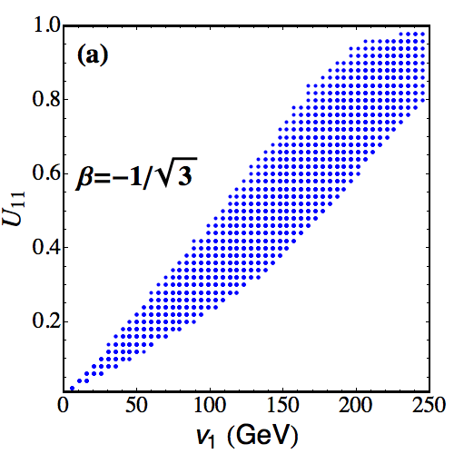
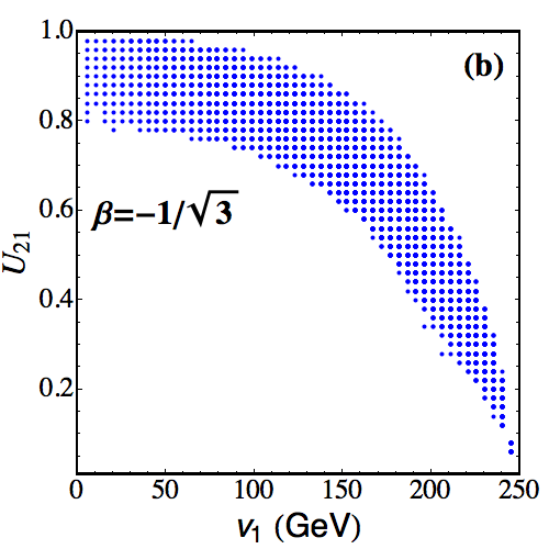
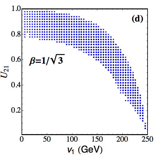
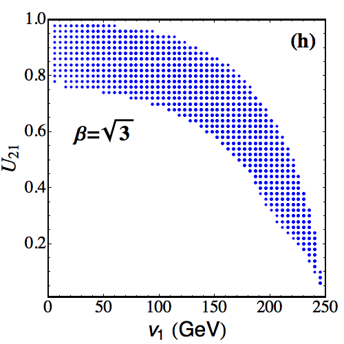
Figure 3: The allowed parameter space in the plane of $v_{1}-U_{11}$ and $v_{1}-U_{21}$ for $v_{3}=2~{}{\rm TeV}$ at the 95% confidence level: (a,b) $\beta=-1/\sqrt{3}$, (c,d) $\beta=+1/\sqrt{3}$, (e,f) $\beta=-\sqrt{3}$, and (g,h) $\beta=+\sqrt{3}$.

Figure 3 displays the 95% confidence level allowed regions for $v_{3}=2{~{}\rm TeV}$, respectively, with different choices of $\beta$: (a,b) $\beta=-1/\sqrt{3}$, (c,d) $\beta=+1/\sqrt{3}$, (e,f) $\beta=-\sqrt{3}$, and (g,h) $\beta=+\sqrt{3}$. First, we note that the allowed parameter space is not sensitive to $\beta$. Even though the electronic charges of new resonances depend on the value of $\beta$, the loop effects of those new resonances are suppressed by the large value of $v_{3}$, yielding a less sensitive dependence on $\beta$.

Second, the $U_{11}$ parameter depends mainly linearly on $v_{1}$ in the decoupling limit, i.e. $U_{11}\simeq v_{1}/v$; see Eq. (15). The dependence of $U_{21}$ on $v_{1}$ is in the form of $\sqrt{1-v_{1}^{2}/v^{2}}$; see Fig. 3. The bands of allowed parameter space are mainly from the $\kappa_{\gamma}$ data, of which the $W$-boson contribution dominates. The $W$-boson contribution to the $H\gamma\gamma$ anomalous coupling, $\frac{v_{1}U_{11}+v_{2}U_{21}}{v^{2}}A_{1}^{h}(\tau_{W})$, is close to the SM value, i.e. $(v_{1}U_{11}+v_{2}U_{21})/v^{2}\sim 1$. Together with the condition $v_{1}^{2}+v_{2}^{2}=v^{2}$, it yields the bands shown in Fig. 3, which clearly demonstrates the competition between $v_{1}$ and $v_{2}$.

3.2 $pp\to h\to Z\gamma$ channel

With the parameter regions allowed by the Higgs boson signal strength, we can give the prediction of $\sigma(pp\to h\to Z\gamma)$ in the 331 model. The $Z\gamma$ decay mode is complementary to the $\gamma\gamma$ mode as the $Z\gamma$ is sensitive to the weak eigenstate particles inside the loop while the $\gamma\gamma$ mode just probes charged particles inside the loop. Combining both $Z\gamma$ and $\gamma\gamma$ modes would help deciphering the nature of the Higgs boson Cao et al. (2016, 2015).

The signal strength relative to the SM expectation,

$$R_{Z\gamma}\equiv\frac{\sigma(pp\to h\to Z\gamma)}{\sigma(pp\to h\to Z\gamma)_{\rm SM}}=\left(\frac{g_{hZ\gamma}}{g_{hZ\gamma}^{\rm SM}}\right)^{2},$$ (103)

is shown in Fig. 4 as a function of $v_{1}$ with fixed $v_{3}=2{\rm~{}TeV}$. The signal strength $R_{Z\gamma}$ is not sensitive to either $\beta$ or $v_{1}$. The $R_{Z\gamma}$ can be enhanced as large as $\sim 1.2$. The cancellation between the contribution of the new fermions and gauge bosons can also reduce the signal strength. For example, we observe that the signal strength are typically larger than $\sim 0.6$ for $\beta=\pm 1/\sqrt{3}$ while larger than $\sim 0.5$ for $\beta=\pm\sqrt{3}$. If the $Z\gamma$ mode is found to be suppressed sizably, say $R_{Z\gamma}<0.6$, then one can exclude the option of $\beta=\pm 1/\sqrt{3}$.

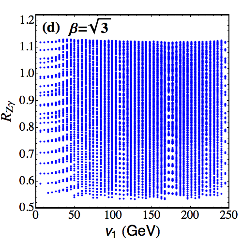
Figure 4: The signal strength $R_{Z\gamma}$ as a function of $v_{1}$ for different choices of $\beta$ and $v_{3}=2{~{}\rm TeV}$ in the parameter space allowed by single Higgs boson measurements at 95% confidence level.

3.3 Higgs-boson pair production

Figure 5: The triangle and box Feynman diagram of double Higgs boson production in the SM.

The double Higgs boson production has drawn a lot of attentions because it is the golden channel to directly measure the triple Higgs-boson self-interaction in the SM, and therefore, tests the electroweak symmetry breaking mechanism. As the Higgs boson does not carry any color, they are produced in pair through the triangle loop and box loop shown in Fig. 5. The production rate in the SM is small mainly due to the large cancellation between the triangle and box diagrams which can be easily understood from the low energy theorem Shifman et al. (1979); Kniehl and Spira (1995). At the LHC with an center of mass energy of $14{~{}\rm TeV}$, the production cross section is about $40~{}{\rm fb}$, which cannot be measured owing to the small branching ratio of the Higgs boson decay and large SM backgrounds Shao et al. (2013). However, in new physics models, the Higgs trilinear coupling can significantly deviate from the SM value. It then could enhance the di-Higgs production make it testable at the LHC. Therefore, it is important to study how large can the cross section of the double Higgs boson production be considering all the constraints from the single Higgs boson measurements.

The squared amplitude of $gg\to hh$ in the SM is given by Dawson et al. (2015)

$$|{\cal M}|^{2}_{\rm SM}=\frac{\alpha_{s}^{2}\hat{s}^{2}}{\pi^{2}v^{4}}\bigg{[}\bigg{|}{3m_{h}^{2}\over{\hat{s}}-m_{h}^{2}}F_{\bigtriangleup}+F_{\Box}\bigg{|}^{2}+\left|G_{\Box}\right|^{2}\bigg{]},$$ (104)

where $F_{\bigtriangleup}\equiv F_{\bigtriangleup}({\hat{s}},{\hat{t}},m_{h}^{2},m_{t}^{2})$, $F_{\Box}\equiv F_{\Box}({\hat{s}},{\hat{t}},m_{h}^{2},m_{t}^{2})$ and $G_{\Box}\equiv G_{\Box}({\hat{s}},{\hat{t}},m_{h}^{2},m_{t}^{2})$ are the form factors Plehn et al. (1996) with $\hat{s}$ and $\hat{t}$ the canonical Mandelstam variables. $G_{\Box}$ represents the $d$-wave contribution, which is negligible Dawson et al. (2013). In the large $m_{t}$ limit, $F_{\bigtriangleup}\to+2/3$ and $F_{\Box}\to-2/3$, therefore, they tend to cancel around the energy threshold of Higgs boson pairs, say $\sqrt{\hat{s}}\sim 4m_{h}^{2}$. In the 331 model, the top Yukawa coupling and Higgs trilinear coupling are

$$y_{htt} = \frac{U_{11}v}{v_{1}}\left(\frac{m_{t}}{v}\right)\equiv c_{t}\left(\frac{m_{t}}{v}\right)\equiv c_{t}y_{htt}^{\rm SM},$$ (105)

$$\lambda_{hhh} = \left(1+\frac{kv_{1}v_{2}U_{31}^{2}}{m_{h}^{2}}\right)\frac{3m_{h}^{2}}{v}\equiv c_{3}\frac{3m_{h}^{2}}{v}=c_{3}\lambda_{hhh}^{\rm SM}.$$ (106)

Therefore, the squared amplitude of $gg\to hh$ is

$$|{\cal M}|^{2}=\frac{\alpha_{s}^{2}\hat{s}^{2}}{\pi^{2}v^{4}}\bigg{[}\bigg{|}{3m_{h}^{2}\over{\hat{s}}-m_{h}^{2}}c_{3}c_{t}F_{\bigtriangleup}+c_{t}^{2}F_{\Box}\bigg{|}^{2}+\left|c_{t}^{2}G_{\Box}\right|^{2}\bigg{]}.$$ (107)

Again, we consider the signal strength relative to the SM expectation $R_{hh}$ defined as following:

$$R_{hh}=\frac{\sigma(pp\to hh)}{\sigma(pp\to hh)_{SM}}.$$ (108)

Figure 6 displays the signal strength $R_{hh}$ as a function of $v_{1}$ in the parameter space allowed by the single Higgs production measurement at the 95% confidence level. Similar to the case of $R_{Z\gamma}$, the signal strength $R_{hh}$ is not sensitive to $\beta$. That is simply because the di-Higgs production is mainly from the QCD, Yukawa and Higgs trilinear coupling, which is not sensitive to $\beta$ at all. The loop corrections from new quarks inside the triangle and box diagrams could enhance $R_{hh}$ and the maximum of $R_{hh}$ is around 3. Unfortunately, it is still not enough to observe the $hh$ pair production with such an enhancement at the high luminosity LHC with an integrate luminosity of $3000{\rm~{}fb^{-1}}$ Collaboration (2014); for example, the red line in Fig. 6 represents the $5\sigma$ discovery potential of the HL-LHC. The future hadron-hadron circular collider (FCC-hh) or the super proton-proton collider (SppC), designed to operate at the energy of 100 TeV, can easily probe most of the parameter space through the $hh$ pair production Bicer et al. (2014); Group (2015). It is shown that the di-Higgs signal can be discovered if $R_{hh}>0.07$, which covers also entire parameter space of the 331 model.

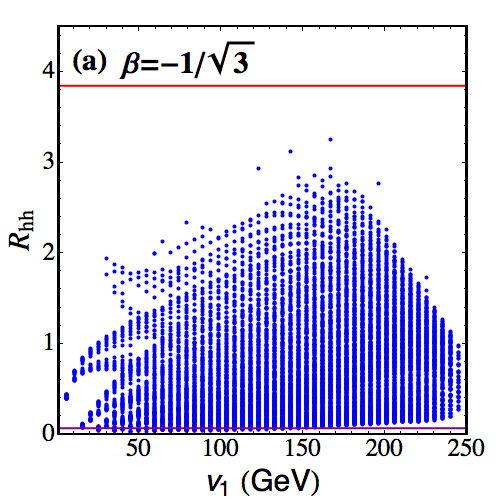
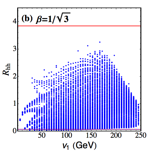
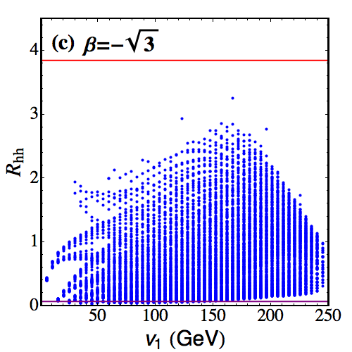
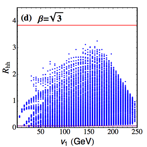
Figure 6: The signal strength $R_{hh}$ as a function of $v_{1}$ for different choices of $\beta$ and $v_{3}=2{~{}\rm TeV}$ in the parameter space allowed by single Higgs boson measurements at the 95% confidence level. The red line is the 5$\sigma$ discovery limit for the HL-LHC. While the purple line shows the discovery potential of the di-Higgs signal at the 100 TeV FCC-hh or SppC with an integrated luminosity 6 and 30 ab^-1, respectively.

4 Phenomenology of $Z^{\prime}$

The 331 model consists of new fermions, gauge bosons and scalars, which yields very rich collider phenomenologies. In this section we first examine the phenomenology of new neural gauge boson $Z^{\prime}$ at the LHC and then discuss other resonances after.

4.1 Production of the $Z^{\prime}$ boson

At the LHC the $Z^{\prime}$ boson is produced singly through quark annihilation processes. The interaction of the $Z^{\prime}$ boson to the fermion $f$ is

$$\mathcal{L}_{f}=Z^{\prime}_{\mu}\,\bar{f}\,\gamma^{\mu}(g_{L}P_{L}+g_{R}P_{R})f,$$ (109)

where $P_{L,R}=(1\mp\gamma_{5})/2$ are the usual chirality projectors. Without loss of generality we assume $V_{L}=V_{\rm CKM}$ and the rotation matrix of up-type quark $U_{L}$ being the Identity matrix. Therefore, the couplings of $Z^{\prime}$-boson to fermions, $g_{L}$ and $g_{R}$, depends only on $\beta$. The relevant Feynman rules are given in Appendix A.

At the LHC, the cross section of $pp\to Z^{\prime}\to XY$ is

$$\sigma_{pp\to V^{\prime}\to\bar{f}f^{\prime}}=\sum_{\{ij\}}\int_{\tau_{0}}^{1}\frac{d\,\tau}{\tau}\cdot\frac{1}{s}\frac{d\,\mathcal{L}_{ij}}{d\,\tau}\cdot[\hat{s}\,\hat{\sigma}_{ij\to V^{\prime}\to\bar{f}f^{\prime}}(\hat{s})]\,,$$ (110)

where $X$ and $Y$ denote the decay products of the $Z^{\prime}$ boson, $\sqrt{s}$ is the total energy of the incoming proton-proton beam, $\sqrt{\hat{s}}$ is the partonic center-of-mass (c.m.) energy and $\tau\equiv\hat{s}/s$. The lower limit of $\tau$ variable is determined by the kinematics threshold of the $Z^{\prime}$ production, i.e. $\tau_{0}=M_{Z^{\prime}}^{2}/s$. The parton luminosity $\frac{1}{s}\frac{d\,\mathcal{L}_{ij}}{d\,\tau}$ is defined as

$$\frac{1}{s}\frac{d\,\mathcal{L}_{ij}}{d\,\tau}=\frac{1}{1+\delta_{ij}}\frac{1}{s}\int_{\tau}^{1}\frac{d\,x}{x}[f_{i}^{(a)}(x)f_{j}^{(b)}(\tau/x)+f_{j}^{(a)}(x)f_{i}^{(b)}(\tau/x)]\,,$$ (111)

where $i$ and $j$ denote the initial state partons and $f_{i}^{(a)}(x)$ is the parton distribution of the parton $i$ inside the hadron $a$ with a momentum fraction of $x=p_{i}/p_{a}$. Using the narrow width approximation (NWA) one can factorize the $pp\to Z^{\prime}\to XY$ process into the $Z^{\prime}$ production and the $Z^{\prime}$ decay,

$$\sigma_{pp\to Z^{\prime}\to XY}=\left(\sum_{\{ij\}}\int_{\tau_{0}}^{1}\frac{d\,\tau}{\tau}\cdot\frac{1}{s}\frac{d\,\mathcal{L}_{ij}}{d\,\tau}\cdot[\hat{s}\,\hat{\sigma}_{ij\to Z^{\prime}}(\hat{s})]\right)\,\times{\rm Br}(Z^{\prime}\to XY),$$ (112)

where the branching ratio (Br) is defined as ${\rm Br}(Z^{\prime}\to XY)=\Gamma(Z^{\prime}\to XY)/\Gamma_{\rm tot}.$ As to be shown later, the decay width of $Z^{\prime}$ boson in most of the allowed parameter space are much smaller than their masses, which validates the NWA adapted in this work. The partonic cross section of the $Z^{\prime}$ production is

$$\hat{\sigma}_{ij\to V^{\prime}}(\hat{s})=\frac{\pi}{6\hat{s}}(g_{L}^{2}+g_{R}^{2})\delta(1-\hat{\tau}),$$ (113)

where $\hat{\tau}\equiv M_{Z^{\prime}}^{2}/\hat{s}$.

We use MadGraph5_aMC@NLO Alwall et al. (2014) to calculate the $Z^{\prime}$ production cross section. The FeynRules Alloul et al. (2014) package is used to generate the 331 model files. Figure 7 displays the $Z^{\prime}$ production cross sections as a function of $M_{Z^{\prime}}$ for different choices of $\beta$. We also plot the $Z^{\prime}$ production cross section in the Sequential Standard Model (SSM) as a reference. The $Z^{\prime}$ boson can be copiously produced at the 8 TeV and 14 TeV LHC. Note that the cross sections of $\beta=\pm\sqrt{3}$ are about one order of magnitude larger than the cross sections of $\beta=\pm 1/\sqrt{3}$. That is due to the large enhancements of the $g_{L}$ and $g_{R}$ couplings for $\beta=\pm\sqrt{3}$, e.g.

$$\beta=+\sqrt{3} : g_{L}^{u,d}\sim-0.37~{},~{}g_{R}^{u}\sim+0.59~{},~{}g_{R}^{d}=-0.30~{},$$ (114)

$$\beta=-\sqrt{3} : g_{L}^{u,d}\sim-0.66~{},~{}g_{R}^{u}\sim-0.59~{},~{}g_{R}^{d}=+0.30~{},$$ (115)

$$\beta=+\tfrac{1}{\sqrt{3}} : g_{L}^{u,d}\sim-0.18~{},~{}g_{R}^{u}\sim+0.08~{},~{}g_{R}^{d}=-0.04~{},$$ (116)

$$\beta=-\tfrac{1}{\sqrt{3}} : g_{L}^{u,d}\sim-0.22~{},~{}g_{R}^{u}\sim-0.08~{},~{}g_{R}^{d}=+0.04~{}.$$ (117)

That leads to an enhancement factor $\sim 10$ in the $Z^{\prime}$ production cross section in the case of $\beta=\pm\sqrt{3}$.

Figure 7: The production cross sections of the $Z^{\prime}$ boson as a function of $M_{Z^{\prime}}$ for different choices of $\beta$ at the 8 TeV LHC (a) and the 14 TeV LHC (b). For comparison we also plots the production cross section of a sequential $Z^{\prime}$ boson (SSM).

4.2 Decay of the $Z^{\prime}$ boson

Now consider the $Z^{\prime}$ boson decay. The decay channels can be classified into four categories. First, it can decay to a pair of fermion and anti-fermion. Second, it can decay into a pair of gauge boson, owing to non-abelian interaction. To be more specific, it could decay to $YY$ and $VV$ pairs, but cannot decay into a pair of $WW$ bosons. It is due to $SU(3)$ gauge group, whose structure constant $f^{128}=0$. The decay mode $Z^{\prime}\to ZZ$ is also forbidden by CP symmetry of the 331 model. Third, it may decay into a pair of Higgs bosons. The case can be further classified into two subcategories: one is charged Higgs boson pairs in the final states, the other involves one CP-even Higgs boson and one CP-odd Higgs boson. Last, the $Z^{\prime}$ may decay into a pair of gauge boson and Higgs boson as well.

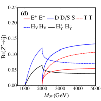
Figure 8: Decay branching ratios of $Z^{\prime}$ with respect to $M_{Z^{\prime}}$. (a) and (b) correspond to $\beta=-1/\sqrt{3}$, while (c) and (d) correspond to $\beta=+1/\sqrt{3}$. (a) and (c) include the SM particles, while (b) and (d) include the 331 model particles. Here we use a different notation of the charged scalar, where the electric charge is expressed apparently and a subscript is added to represent the corresponding charged scalar. The heavy fermion masses are chosen to be $1000\,{\rm GeV}$, and the charged Higgs boson masses are chosen to be $500\,{\rm GeV}$.

Figures 8 and 9 display the branching ratio of different decay modes of the $Z^{\prime}$ boson as a function of $M_{Z^{\prime}}$ in different 331 models. The branching ratio depends on many parameters. A global fitting has to be carried out to fully understand the model parameter space, but for illustration, we choose $v_{1}=200\,{\rm GeV}$ and fix $M_{H^{\pm Q_{V}}}=1.3\,{\rm TeV}$ and $M_{H^{\pm Q_{Y}}}=1.4\,{\rm TeV}$ in this work by tuning $\lambda_{13}$ and $\lambda_{23}$ for different $v_{1}$ and $v_{3}$. We drop those decay modes with a branching ratio less than 1 percent. For example, the decay modes involving the $H^{\pm}$, $H_{2}$ and $H_{0}$ scalars will be highly suppressed, e.g. $Z^{\prime}\to H^{+}H^{-}$, $Z^{\prime}\to hH_{0}$, $Z^{\prime}\to H_{3}H_{0}$, $Z^{\prime}\to H_{2}H_{0}$, and $Z^{\prime}\to ZH_{2}$, etc. That is owing to the fact that the nearly degenerate masses of $H^{\pm}$, $H_{2}$ and $H_{0}$ is slightly smaller or even larger than $M_{Z^{\prime}}$, which leads to a large suppression from the phase space. Also, the decay modes involving one $Z$ boson and one neutral Higgs boson are highly suppressed by the small coupling, e.g. $Z^{\prime}\to Zh$ and $Z^{\prime}\to ZH_{3}$, etc.

Note that the specific value of $v_{1}$ is not important. The $v_{1}$ will affect both the mass of $V$ or $Y$ and the couplings of $ZH^{+Q_{V}}H^{-Q_{V}}$ and $ZH^{+Q_{Y}}H^{-QY}$, however, its effect is overwhelmed by $v_{3}$. As a consequence, the branching ratios alter less than 1 percent while varying $v_{1}$, and therefore, we just consider one value of $v_{1}$ throughout this work.

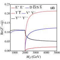
Figure 9: Decay branching ratios of $Z^{\prime}$ with respect to $M_{Z^{\prime}}$. (a) and (b) correspond to $\beta=-\sqrt{3}$, while (c) and (d) correspond to $\beta=\sqrt{3}$. (a) and (c) include the SM particles, while (b) and (d) include the 331 model particles. The heavy fermions’ masses are chosen to be $1000\,{\rm GeV}$, and the charged Gauge bosons’ masses are determined by $Z^{\prime}$ mass (82).

Different 331 models share a few common features of the branching ratio of $Z^{\prime}$-boson decay, as depicted in Figs. 8 and 9. First, the decay of $Z^{\prime}$ boson into a pair of the SM fermions dominate for a light $Z^{\prime}$ boson. It is worth mentioning that the decay of the $Z^{\prime}$ boson into a pair of neutrinos, $Z^{\prime}\to\nu_{l}\bar{\nu}_{l}$, is absent in the case of $\beta=\sqrt{3}$ as the coupling is zero. Second, for a $Z^{\prime}$ boson in the medium mass region, the decay modes of the $Z^{\prime}$ boson into heavy leptons, heavy quarks and heavy charged Higgs bosons, if allowed kinematically, will contribute sizably and compete with those light SM fermion modes. Third, when $M_{Z^{\prime}}$ is very large, we can ignore the masses of decay products. The heavy quarks is the predominant decay channel of the $Z^{\prime}$ boson. All the decay branching ratios of $Z^{\prime}\to E_{\ell}E_{\ell}$ ($\ell=e,\mu,\tau$) are identical, and so do the $Z^{\prime}\to DD$ and $Z^{\prime}\to SS$ channels. The decay of $Z^{\prime}\to TT$ deviates from the $Z^{\prime}\to DD/SS$ channels since the $T$ quark lives in the anti-triplet representation of the $SU(3)_{L}$ group. Owing to the same reason, the branching ratio of the $Z^{\prime}\to t\bar{t}$ channel is not identical to that of $Z^{\prime}\to u\bar{u}(c\bar{c})$. Similarly, the decay of $Z^{\prime}\to b\bar{b}$ is also not identical to the decay of $Z^{\prime}\to d\bar{d}(s\bar{s})$.

Note that $M_{Z^{\prime}}>2M_{V(Y)}$ for $\beta=\pm\sqrt{3}$ and $M_{Z^{\prime}}<2M_{V(Y)}$ for $\beta=\pm 1/\sqrt{3}$. As a consequence, the $Z^{\prime}\to VV(YY)$ channel only opens for $\beta=\pm\sqrt{3}$. We plot the branching ratio of the $Z^{\prime}\to H^{+Q_{V(Y)}}H^{-Q_{V(Y)}}$ mode for $\beta=\pm 1/\sqrt{3}$ but not for $\beta=\pm\sqrt{3}$; see the blue and red dotted curves in Fig. 8. Note that it is not because the partial decay width of $Z^{\prime}\to H^{+Q_{V(Y)}}H^{-Q_{V(Y)}}$ is small or absent for $\beta=\pm\sqrt{3}$; on the contrary, the partial width is larger in the case of $\beta=\pm\sqrt{3}$ than in the case of $\beta=\pm 1/\sqrt{3}$. However, the total width of the $Z^{\prime}$ also increases dramatically for $\beta=\pm\sqrt{3}$ such that the branching ratio of $Z^{\prime}\to H^{+Q_{V(Y)}}H^{-Q_{V(Y)}}$ mode is highly suppressed. As a consequence, it is difficult to detect the $Z^{\prime}$ through a pair of $H^{\pm Q_{V(Y)}}$ scalar in the case of $\beta=\pm\sqrt{3}$.

Figure 10 plots the total width of the $Z^{\prime}$ as a function of $M_{Z^{\prime}}$ in different 331 models with the masses of new physics particles specified above. The total width of $Z^{\prime}$ boson varies greatly for different $\beta$’s. For example, the $Z^{\prime}$ boson exhibits a narrow width for $\beta=\pm 1/\sqrt{3}$; while the width of $Z^{\prime}$ boson for $\beta=\pm\sqrt{3}$ is much broader than the case of $\beta=\pm 1/\sqrt{3}$. Of course the decay width depends on whether or not the decay channels involving new physics particles. For illustration, we also plot the sum of partial widths of the $Z^{\prime}$ decaying into a pair of SM fermions in Fig. 10, depicted by the dashed curves. One should treat the dashed curve as the lower limit of the $Z^{\prime}$-boson width. It is clear that, owing to the large couplings of $Z^{\prime}$ boson to SM fermions for $\beta=\pm\sqrt{3}$, the $Z^{\prime}$ boson in the $\beta=\pm\sqrt{3}$ models exhibit much larger width than in the $\beta=\pm 1/\sqrt{3}$ models.

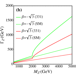
Figure 10: Total width of $Z^{\prime}$ with respect to $M_{Z^{\prime}}$ in different versions of the 331 model. (a) and (b) correspond to $\beta=\pm 1/\sqrt{3}$ and $\beta=\pm\sqrt{3}$ respectively. The solid lines represent the total width including all the decay modes. While the dashed lines stand for the total width that the $Z^{\prime}$ boson decays only the SM fermions, which is a lowest limit of the real total width.

4.3 $M_{Z^{\prime}}$ constraint from the dilepton search at the LHC

The constraint on $M_{Z^{\prime}}$ is obtained from the Drell-Yan channel $pp\to Z^{\prime}\to e^{+}e^{-}/\mu^{+}\mu^{-}$ at the LHC. Ref. Salazar et al. (2015) studied the constraint on $M_{Z^{\prime}}$ in different 331 models from the dilepton signal using the 8 TeV LHC data Aad et al. (2014) and obtained a typical bound of $M_{Z^{\prime}}\gtrsim 3$ TeV. In this work we consider the recent negative result of dilepton searches at the 14 TeV LHC collaboration (2016) to set a constraint on $M_{Z^{\prime}}$ in the 331 models. The cross sections of $pp\to Z^{\prime}\to\ell^{+}\ell^{-}$ ($\ell=e,\mu$) are plotted in Fig. 11 as a function of $M_{Z^{\prime}}$. The exclusion limit on $\sigma(pp\to Z^{\prime}\to\ell^{+}\ell^{-})$ is also shown; see the black curve. Two scenarios of $Z^{\prime}$ decay is considered. First, we consider the case that the $Z^{\prime}$ boson decays only into a pair of SM fermions, therefore, $\sigma(pp\to Z^{\prime}\to\ell^{+}\ell^{-})$ is maximumly enhanced and that leads to stronger constraints on $M_{Z^{\prime}}$. For example, it yields $M_{Z^{\prime}}\gtrsim 4.4$ TeV for $\beta=-1/\sqrt{3}$ and $M_{Z^{\prime}}\gtrsim 4$ TeV for $\beta=+1/\sqrt{3}$, respectively; see Fig. 11(a). For $\beta=\pm\sqrt{3}$, the $Z^{\prime}$ boson with a mass smaller than 5 TeV is completely excluded. Second, we allow the $Z^{\prime}$ boson can also decay into a pair of heavy fermions and fix all the heavy fermion masses to be 1 TeV. The cross section $\sigma(pp\to Z^{\prime}\to\ell^{+}\ell^{-})$ is slightly smaller than the first case; see Fig. 11 (b). That yields a slightly weakened bound on $M_{Z^{\prime}}$: $M_{Z^{\prime}}\gtrsim 4.2~{}{\rm TeV}$ for $\beta=-1/\sqrt{3}$ and $M_{Z^{\prime}}\gtrsim 3.6~{}{\rm TeV}$ for $\beta=+1/\sqrt{3}$, respectively. Again, a $Z^{\prime}$ boson with mass less than 5 TeV in the $\beta=\pm\sqrt{3}$ models is already ruled out.

Figure 11: Constraint on $M_{Z^{\prime}}$ in different versions of 331 model, where the black line shows the 95% C.L. limit on the $Z^{\prime}$ production cross section times branching ratio to two leptons as a function of $M_{Z^{\prime}}$ from collaboration (2016). (a) is assuming $Z^{\prime}$ only decays to SM fermions, while (b) assumes $Z^{\prime}$ can also decay to the heavy fermions with fermion’s masses all set to be 1 TeV.

We choose two benchmark masses of the $Z^{\prime}$ boson in the study: $M_{Z^{\prime}}=4~{}{\rm TeV}$ in the $\beta=\pm 1/\sqrt{3}$ models and $6~{}{\rm TeV}$ in the $\beta=\pm\sqrt{3}$ models, to respect the current LHC bounds. For simplicity, we consider the $Z^{\prime}$ boson decaying only into the SM fermions.

4.4 Search for $Z^{\prime}$ through $A_{FB}$ at the LHC

The width of $Z^{\prime}$ boson is very broad when $\beta=\pm\sqrt{3}$ due to its large couplings with the fermions. It is hard to probe such a broad resonance through the usual bump search. For illustration, Fig. 12 plots the invariant mass distribution of the charged-lepton pair $m_{\ell\ell}$, which is equal to the center of mass energy of the hard scattering $\sqrt{\hat{s}}$ at the tree level, in the process of $pp\to\gamma/Z/Z^{\prime}\to\ell^{+}\ell^{-}$ for both $\beta=\pm\sqrt{3}$ and $\beta=\pm 1/\sqrt{3}$ models at the 14 TeV LHC: (a) $M_{Z^{\prime}}=4~{}{\rm TeV}$ and (b) $M_{Z^{\prime}}=6~{}{\rm TeV}$. The $Z^{\prime}$ bosons in the $\beta=\pm 1/\sqrt{3}$ models (purple and blue curves) appear as a peak on top of the SM background (black curve), but the $Z^{\prime}$ bosons in the $\beta=\pm\sqrt{3}$ models (green and red curves) display a very broad bump on top of the SM background. It is very hard to detect such a non-resonance shape experimentally. In addition, the distribution will be distorted by the detector effects which make the detection more challenging.

Fortunately, the so-called Forward-Backward Asymmetry ($A_{\rm FB}$) of the charged lepton provides us a powerful tool to probe a “fat” $Z^{\prime}$ boson at the LHC Accomando et al. (2016). The $A_{\rm FB}$ of the charged lepton is defined as the difference of the fractions that the charged lepton appears in the forward and backward regimes of the detector, i.e.

$$A_{FB}(\hat{s})=\frac{\sigma_{F}(\hat{s})-\sigma_{B}(\hat{s})}{\sigma_{F}(\hat{s})+\sigma_{B}(\hat{s})},$$ (118)

where $\hat{s}$ is the lepton pair invariant mass squared, $\sigma_{F}$ and $\sigma_{B}$ are the cross section of the charged lepton in the forward and backward regimes, respectively. We call the charged lepton in the forward region when its polar angle with respect to the quark direction is from 0 to $\pi/2$ in the center-of-mass-frame of the di-lepton system, and in the backward region when the angle is from $\pi/2$ to $\pi$.

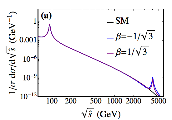
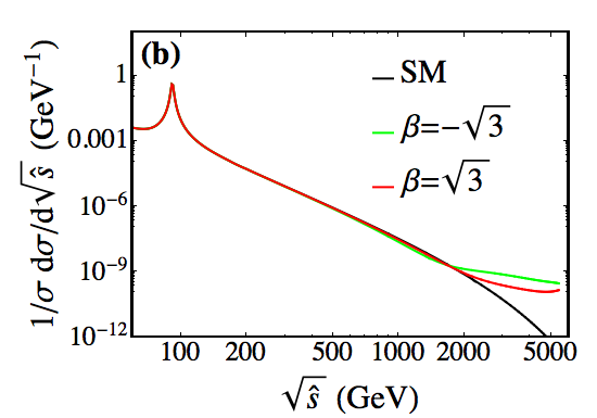
Figure 12: Invariant mass ($m_{\ell^{+}\ell^{-}}$) distribution of lepton pair in the process of $pp\to\gamma/Z/Z^{\prime}\to\ell^{+}\ell^{-}$ at the 14 TeV LHC in the SM (black) and various 331 model: (a) $M_{Z^{\prime}}=4\,{\rm TeV}$ and (b) $M_{Z^{\prime}}=6\,{\rm TeV}$. The $Z^{\prime}$ boson decaying into a pair of the SM fermions is understood.

At the partonic level the $A_{\rm FB}$ is given by

$$A_{FB}(\hat{s})=\frac{3}{4}\times\frac{\sum_{i,j=1}^{N}C_{A}^{ij}P_{ij}(\hat{s})}{\sum_{i,j=1}^{N}C_{S}^{ij}P_{ij}(\hat{s})},$$ (119)

where $N$ stands for the numbers of gauge bosons involved involved in the process, $C_{A}^{ij}$ ($C_{S}^{ij}$) denotes the parity antisymmetric (symmetric) coefficient, respectively. Both coefficients are a function of the chiral gauge couplings of the $i$-boson to the quark ($q_{L/R}^{i}$ ) and lepton ($l_{L/R}^{i}$), which are listed as follows:

$$C_{A}^{ij} = (q_{L}^{i}q_{L}^{j}-q_{R}^{i}q_{R}^{j})(l_{L}^{i}l_{L}^{j}-l_{R}^{i}l_{R}^{j}),$$ (120)

$$C_{S}^{ij} = (q_{L}^{i}q_{L}^{j}+q_{R}^{i}q_{R}^{j})(l_{L}^{i}l_{L}^{j}+l_{R}^{i}l_{R}^{j}).$$ (121)

The $\hat{s}$ dependent variable $P_{ij}(\hat{s})$ arises from the propagators of gauge bosons involved in the process

$$P_{ij}(\hat{s})=\frac{(\hat{s}-M_{i}^{2})(\hat{s}-M_{j}^{2})+M_{i}M_{j}\Gamma_{i}\Gamma_{j}}{[(\hat{s}-M_{i}^{2})^{2}+M_{i}^{2}\Gamma_{i}^{2}][(\hat{s}-M_{j}^{2})^{2}+M_{j}^{2}\Gamma_{j}^{2}]},$$ (122)

where $M_{i}$ and $\Gamma_{i}$ is the mass and width of the $i$-boson, respectively.

Figure 13 shows the $A_{\rm FB}$ distribution as a function of $\sqrt{\hat{s}}$ in the SM and the two benchmark 331 models: (a) $M_{Z^{\prime}}=4~{}{\rm TeV}$ in the $\beta=\pm 1/\sqrt{3}$ models and (b) 6 TeV in the $\beta=\sqrt{3}$ models. The black (red, green, purple, blue) curve denotes the SM ($\beta=+\sqrt{3}$, $\beta=-\sqrt{3}$, $\beta=+1/\sqrt{3}$, $\beta=-1/\sqrt{3}$), respectively. When $\sqrt{\hat{s}}$ is larger than 200 GeV, the $A_{\rm FB}$ approaches 0.6 in the SM as there is no other heavier gauge bosons. But if there is a $Z^{\prime}$ boson, the $A_{\rm FB}$ can deviate from the SM prediction. The deviation depends on the $Z^{\prime}$ boson mass, width and its couplings to the SM fermions.

Figure 13: $A_{FB}$ distribution versus the lepton pair invariant mass $\sqrt{\hat{s}}=m_{\ell^{+}\ell^{-}}$ in the SM and various 331 models at the 14 TeV LHC for (a) $M_{Z^{\prime}}=4\,{\rm TeV}$ and (b) $M_{Z^{\prime}}=6\,{\rm TeV}$ respectively. The width of $Z^{\prime}$ is chosen to be the lowest limit shown in Fig. 10.

In the $\beta=\pm 1/\sqrt{3}$, owing to the narrow width of the $Z^{\prime}$ boson, large deviations occur around $M_{Z^{\prime}}=4~{}{\rm TeV}$; see Fig. 13(a). Thanks to the large width of $Z^{\prime}$ in the $\beta=\pm\sqrt{3}$ models, the $A_{\rm FB}$ can be affected at a energy scale far below $M_{Z^{\prime}}$; see Fig. 13(b). The large deviations occur around half of $M_{Z^{\prime}}$. The $A_{FB}$ distribution has the advantage searching for or excluding a broad resonance even in the case that the collider energy is not enough to see those “fat” resonances directly. We note that, owing to the interference effect between the $Z$ boson and $Z^{\prime}$, the sign of $\beta$ plays an important role in the $A_{\rm FB}$ distributions, which can be used to distinguish different 331 models when collecting enough data.

5 Phenomenology of the $V$ and $Y$ bosons

In this section we study the phenomenology of two unconventional gauge bosons in the 331 models, $V$ and $Y$, at the LHC.

Figure 14: Feynman diagrams for $V(Y)$-pair production, where $q$ stands for SM quarks. In the t-channel diagram $(d)$, we have neglected the flavor mixing in the quark sector and only considered the dominant contribution from $u$ and $d$ quark.

5.1 Production of $V$ and $Y$ bosons

As shown in Fig. 2, the $V$ and $Y$ bosons connect the SM fermions and the exotic fermions that are added to fill the $SU(3)$ (anti)fundamental representation, therefore, the $V$ and $Y$ bosons cannot be produced singly through the Drell-Yan channel as the $Z^{\prime}$ boson. Figure 14 displays a few production channels of $V$ or $Y$ bosons. They can be produced in pair through $V$-$V$-$\gamma/Z/Z^{\prime}$ and $Y$-$Y$-$\gamma/Z/Z^{\prime}$ triple gauge boson interactions (a,b,c) and through the $t$-channel diagram involving a heavy quark (d). They can also be produced in association with a heavy quark production or association with a heavy charged scalar production, e.g. $dg\to DV$ or $ug\to DY$. In the work we focus on the $VV$ and $YY$ pair productions and will study the associated production elsewhere Cao and Zhang (2016).

Figure 15: Inclusive cross sections of $VV$ and $YY$ pair productions as a function of $M_{V}$ and $M_{Y}$ in the 331 models at the 8 TeV LHC (a, c) and 14 TeV LHC (b, d), respectively, where we have set all the heavy quark masses to be 500 GeV. The width of $Z^{\prime}$ is chosen to be the lowest limit shown in Fig. 10.

Figure 15 displays the cross section of $VV$ pair production at the 8 TeV (a) and 14 TeV LHC (b) and $YY$ pair production at the 8 TeV (c) and 14 TeV (d). The cross section of $VV(YY)$ productions depends mainly on the absolute value of $\beta$. The cross sections in the $\beta=\pm\sqrt{3}$ models are larger than those in the $\beta=\pm 1/\sqrt{3}$ models. As mentioned above, the gauge couplings of $Z^{\prime}$ to the SM quarks in the $\beta=\pm\sqrt{3}$ model is larger than the couplings in the $\beta=\pm 1/\sqrt{3}$ models. That yields an enhancement factor of $\sim 10$ to the $VV$ pair production in the case of $\beta=\pm\sqrt{3}$. Another enhancement factor originates from the Breit-Wigner resonance effects. Since $M_{Z^{\prime}}\sim 3M_{V(Y)}$ for $\beta=\sqrt{3}$, the $Z^{\prime}$ propagator in Fig. 14(c) can be produced on mass shell and then exhibit a large Breit-Wigner enhancement. On the other hand, $M_{Z^{\prime}}\sim 1.2M_{V(Y)}$ for $\beta=\pm 1/\sqrt{3}$, therefore, the $Z^{\prime}$ propagator can never be shell, yielding a big suppression in the cross section.

The $YY$ pair production is very similar to the $VV$ pair production. Its production rate is slightly more than the rate of $VV$ pair for the same value of $\beta$. The difference arises from Fig. 14(d), where $V$-pair can only be produced from $d$ quark initial state, while $Y$-pair from $u$ quark initial state due to the $SU(3)$ gauge symmetry. As the parton distribution function of $u$-quarks is larger than that of $d$-quarks, it yields $\sigma(pp\to YY)\gtrsim\sigma(pp\to VV)$.

5.1.1 Unitarity analysis of $u\bar{u}\to YY$ scattering

As a gauge invariant set, the unitarity of the $VV$ or $YY$ pair production process must be maintained considering all the four diagrams. Since the $\beta$ dependence comes only from Fig. 14 (a)-(c). The bad high energy behavior that depends on $\beta$ must disappear within Fig. 14 (a)-(c). A simple example is to consider the amplitude of $u(p_{1})\bar{u}(p_{2})\to Y(p_{3})Y(p_{4})$. We can expand the amplitude into four terms $A^{\gamma}$, $A^{Z}$, $A^{Z^{\prime}}$ and $A^{D}$ given by

$$A^{\gamma} = \frac{g_{\gamma YY}g_{\gamma uu}}{s}\bar{v}(p_{2})\{(-\not\not{p}_{3}+\not\not{p_{4}})\varepsilon^{\ast}(p_{3})\cdot\varepsilon^{\ast}(p_{4})$$

$$-2p_{4}\cdot\varepsilon^{\ast}(p_{3})\not{\varepsilon^{\ast}(p_{4})}+2p_{3}\cdot\varepsilon^{\ast}(p_{4})\not{\varepsilon^{\ast}(p_{3})}\}u(p_{1})\,,$$

$$A^{Z} = \frac{g_{ZYY}}{s-m_{Z}^{2}}\bar{v}(p_{2})\{(-\not\not{p_{3}}+\not\not{p_{4}})\varepsilon^{\ast}(p_{3})\cdot\varepsilon^{\ast}(p_{4})$$

$$-2p_{4}\cdot\varepsilon^{\ast}(p_{3})\not{\varepsilon^{\ast}(p_{4})}+2p_{3}\cdot\varepsilon^{\ast}(p_{4})\not{\varepsilon^{\ast}(p_{3})}\}(g_{L}^{Zuu}+g_{R}^{Zuu})u(p_{1})\,,$$

$$A^{Z^{\prime}} = \frac{g_{Z^{\prime}YY}}{s-m_{Z^{\prime}}^{2}}\bar{v}(p_{2})\{(-\not\not{p_{3}}+\not\not{p_{4}})\varepsilon^{\ast}(p_{3})\cdot\varepsilon^{\ast}(p_{4})$$

$$-2p_{4}\cdot\varepsilon^{\ast}(p_{3})\not{\varepsilon^{\ast}(p_{4})}+2p_{3}\cdot\varepsilon^{\ast}(p_{4})\not{\varepsilon^{\ast}(p_{3})}\}(g_{L}^{Z^{\prime}uu}+g_{R}^{Z^{\prime}uu})u(p_{1})\,,$$

$$A^{D} = -\frac{g_{YDu}}{t-M_{D}^{2}}\bar{v}(p_{2})\not{\varepsilon}^{\ast}(p_{4})P_{L}(\not\not{t}-M_{D})\not{\epsilon^{\ast}(p_{3})}P_{L}u(p_{1})\,,$$

where the related couplings can be found in Appendix A. In the center-of-mass frame of $YY$, the 4-momenta of the particles can be chosen to be

$$p_{1} = (E,0,0,E),~{}~{}p_{2}=(E,0,0,-E),$$

$$p_{3} = (E,\,p\sin\theta,0,p\cos\theta),~{}~{}p_{4}=(E,-p\sin\theta,0,-p\cos\theta)\,,$$

where $E$ is the energy of incoming and outgoing particles, $p$ is the momentum of outgoing heavy gauge bosons and $\theta$ is the scattering angle. In order to check its high energy behavior, we consider the case that both of the outgoing heavy gauge boson $Y$ are longitudinally polarized. Since the incoming fermion $u$ and anti-fermion $\bar{u}$ have opposite helicities, the helicity amplitudes of s-channel and t-channel processes can be easily found to be

$$A^{\gamma}(-+) = g_{\gamma YY}g_{\gamma uu}\frac{4Ep(p^{2}-3E^{2})}{sM_{V}^{2}}\sin\theta\,,$$

$$A^{Z}(-+) = g_{ZYY}g_{Zuu}\frac{4Ep(p^{2}-3E^{2})}{(s-m_{Z}^{2})M_{V}^{2}}\sin\theta\,,$$

$$A^{Z^{\prime}}(-+) = g_{Z^{\prime}YY}g_{Z^{\prime}uu}\frac{4Ep(p^{2}-3E^{2})}{(s-M_{Z^{\prime}}^{2})M_{V}^{2}}\sin\theta\,,$$

$$A^{D}(-+) = g_{YDu}^{2}\frac{2E(2E^{3}\cos\theta+p^{3}-3pE^{2})}{(t-M_{D}^{2})M_{V}^{2}}\sin\theta\,,$$

where $(-+)$ are the helicities of $(u\,\bar{u})$, the Mandelstam variables $s\equiv(p_{1}+p_{2})^{2}$ and $t\equiv(p_{1}-p_{3})^{2}$. As we take the high energy limit, i.e. $\sqrt{s}\gg M_{X}$ ($X=Z$, $Z^{\prime}$ and $D$), each amplitude behaves as follows:

$$A^{\gamma}(-+) = \frac{8(\sqrt{3}\beta+1)e^{2}}{3M_{V}^{2}}s,~{}~{}$$ (123)

$$A^{Z}(-+) = \frac{2[1-(\sqrt{3}\beta+1)s_{W}^{2}](3-4s_{W}^{2})e^{2}}{3s_{W}^{2}c_{W}^{2}M_{V}^{2}}s,~{}~{}$$ (124)

$$A^{Z^{\prime}}(-+) = -\frac{2\sqrt{3}[(\beta+\sqrt{3})s_{W}^{2}-\sqrt{3}]e^{2}}{3s_{W}^{2}c_{W}^{2}M_{V}^{2}}s,~{}~{}$$ (125)

$$A^{D}(-+) = -\frac{4e^{2}}{s_{W}^{2}M_{V}^{2}}s.$$ (126)

It turns out by summing over the Eq. (123)-(125), one cancels out all the $\beta$ dependent terms and leaves only a term $4e^{2}s/s_{W}^{2}M_{V}^{2}$ which exactly cancels Eq. (126).

5.2 Decay of the $V$ and $Y$ bosons

Now we firstly consider the $V$ boson and study its decay branching ratio. The result can be easily applied to the $Y$ boson. The decay modes of the $V$ bosons can be classified into three categories according to the final state particles. In the first class the $V$ boson decays into a SM fermion and a new heavy fermion. In the second class the $V$ boson decays into a SM gauge boson and a new charged scalar. In the third class the $V$ boson decays into a pair of two scalars.

The decay width of the $V$ boson into a pair of fermions is

$$\Gamma(V\to fF) = \frac{N_{c}g^{2}}{96\pi M_{V}^{5}}\Big{(}2M_{V}^{4}-M_{F}^{4}-m_{f}^{4}-M_{V}^{2}m_{f}^{2}-M_{V}^{2}M_{F}^{2}+2M_{F}^{2}m_{f}^{2}\Big{)}$$ (127)

$$\times \lambda^{1/2}\left(M_{V}^{2},m_{f}^{2},M_{F}^{2}\right)$$

where $f$ and $F$ represent the SM and 331 fermion, respectively, $N_{c}=1$ for leptons and $N_{c}=3$ for quarks, and the kinematical function $\lambda$ is defined as $\lambda(x,y,z)=(x-y-z)^{2}-4yz$. Note that the anomaly cancellation condition requires $V\to tT$, therefore, the $tT$ mode is different from the $dD$ and $sS$ modes. Figures 16(a) and 16(b) display the branching ratio of the $V$ boson as a function of $M_{V}$ for different choices of $v_{1}$ and $v_{2}$ parameters. We choose the masses of charged scalars to be 500 GeV while the masses of heavy quarks as 1000 GeV.

Figure 16: Decay branching ratios of $V(Y)$ boson versus $M_{V}(M_{Y})$ for different choices of $v_{1,2}$ parameters: (a,c) $v_{1}=v_{2}=174{~{}\rm GeV}$; (b,d) $v_{1}=200{~{}\rm GeV}$ and $v_{2}=143~{}{\rm GeV}$. The mass of charged scalars is chosen to be 500 GeV and the mass of heavy quarks is 1000 GeV.

The decay width of the $V$ boson into a SM gauge boson and a new charged scalar is

$$\Gamma(V\to U_{i}H^{Q_{i}}) = \frac{\delta_{i}g^{4}\left(v_{3}c_{i3}+v_{i}s_{i3}\right)^{2}}{3072\pi M_{V}^{5}c_{W}^{2}m_{U_{i}}^{2}}\Big{(}M_{V}^{4}+M_{H^{Q_{i}}}^{4}+10M_{V}^{2}m_{U_{i}}^{2}+m_{U_{i}}^{4}$$ (128)

$$- 2M_{V}^{2}M_{H^{Q_{i}}}^{2}-2M_{H^{Q_{i}}}^{2}m_{U_{i}}^{2}\Big{)}\times\lambda^{1/2}\left(M_{V}^{2},m_{U_{i}}^{2},M_{H^{Q_{i}}}^{2}\right)$$

where $U_{1}=Z$, $U_{2}=W$, $Q_{1}=Q_{V}$, $Q_{2}=Q_{Y}$, $\delta_{1}=1$, $\delta_{2}=2$. We learn from Eqs. (27) and (31) that $\left(v_{3}c_{i3}+v_{i}s_{i3}\right)^{2}=(v_{i}v_{3})^{2}/(v_{i}^{2}+v_{3}^{2})\sim v_{i}^{2}$, therefore, ${\rm Br}(V\to ZH^{Q_{V}})$ depends on $v_{1}^{2}$ while ${\rm Br}(V\to WH^{Q_{Y}})$ on $2v_{2}^{2}$. Choosing different $v_{1}$ and $v_{2}$ would change the breaking ratio pattern dramatically. For example, ${\rm Br}(V\to WH^{Q_{Y}})\simeq 2{\rm Br}(V\to ZH^{Q_{V}})$ for choosing $v_{1}=v_{2}=174{~{}\rm GeV}$; see Fig. 16(a). On the other hand, choosing $v_{1}=200~{}{\rm GeV}$ and $v_{2}=143~{}{\rm GeV}$ yields ${\rm Br}(V\to WH^{Q_{Y}})<2{\rm Br}(V\to ZH^{Q_{V}})$ shown in Fig. 16(b).

The $V$ boson can also decay into a pair of scalars, e.g. $V\to hH^{Q_{V}}$, $V\to H_{0,2,3}H^{Q_{V}}$ and $V\to H^{\pm}H^{Q_{Y}}$, if kinematically allowed. If we neglect the small mixing of $\xi_{\chi}$ with $\xi_{\rho}$ and $\xi_{\eta}$, the decay mode $V\to H_{3}H^{Q_{V}}$ is absent. In addition, the decay modes $V\to H_{2}H^{Q_{V}}$, $V\to H_{0}H^{Q_{V}}$ and $V\to H^{\pm}H^{Q_{Y}}$ will be suppressed by the phase space factor. Therefore we only consider $V\to hH^{Q_{V}}$ for a light $V$ boson. The partial decay width is

$$\Gamma(V\to hH^{Q_{V}}) = \frac{g^{2}U_{11}^{2}s_{13}^{2}}{192\pi M_{V}^{5}}\Big{(}M_{V}^{4}+M_{H^{Q_{V}}}^{4}+m_{h}^{4}-2M_{V}^{2}M_{H^{Q_{V}}}^{2}-2M_{V}^{2}m_{h}^{2}-2M_{H^{Q_{V}}}^{2}m_{h}^{2}\Big{)}$$ (129)

$$\times \lambda^{1/2}\left(M_{V}^{2},m_{h}^{2},M_{H^{Q_{V}}}^{2}\right),$$

where the approximation of $U_{11}\sim v_{1}/v$ is used to simplify the calculation. Comparing Eqs. 128 and 129, we note that $\Gamma(V\to hH^{Q_{V}})\sim\Gamma(V\to ZH^{Q_{V}})$ when $M_{V}\gg m_{h},m_{Z}$, which is a consequence of the Equivalence Theorem. While $M_{V}$ is not too large, the contribution from the transverse mode of $Z$ can be important and leads to $\Gamma(V\to ZH^{Q_{V}})>\Gamma(V\to hH^{Q_{V}})$.

Figures 16(c) and 16(d) shows the decay branching ratio of the $Y$ boson, which is similar to that of $V$ with the only difference is about the $v_{1}$ dependence of the second and third category.

5.3 Collider signatures of the $V$ and $Y$ bosons

Now consider the phenomenology of the $VV$ and $YY$ pair production. As mentioned above, there will be a DM candidate or LLP in the 331 models, depending on $\beta$. Table 3 shows the possible DM candidate or LLP in different 331 models. We will discuss collider signatures of $VV$ and $YY$ pair productions.

Note that the $V$ and $Y$ bosons are almost degenerate and $\big{|}M_{Y^{\pm Q_{Y}}}-M_{V^{\pm Q_{V}}}\big{|}\ll m_{W}$; see Eq. (81). If the $Y$ boson is the lightest particle, then the $V$ boson can only decay into a $Y$ boson and an off-shell $W$ boson which will further decay into a pair of the SM fermions. It is indeed a three-body decay, i.e. $V\to YW^{*}\to Yq\bar{q}^{\prime}$ or $V\to YW^{*}\to Y\ell^{+}\nu$. The SM quarks and charged leptons in $V$ boson decay tend to fail the experimental cuts simply because they are not energetic. The same conclusion also applies to the case of the $V$ boson being the lightest particle. If other particle is the DM candidate, then the $V$ and $Y$ bosons decay in the way as shown in Fig. (16).

Table 3: Collider signatures of $VV$ ($YY$) pair productions for $\beta=\pm 1/\sqrt{3}$ and DM candidate, where the star symbol in the superscript denotes the particle being off-shell.

	DM candidate	Production channel	Collider signature
$\beta=-\frac{1}{\sqrt{3}}$	$Y$	$VV$	$W^{*+}W^{*-}+{E\!\!\!\!/}_{T}$
		$YY+j(\gamma)$	$j/\gamma+{E\!\!\!\!/}_{T}$
	$H^{Q_{Y}}$	$VV$	$WW+{E\!\!\!\!/}_{T}$
		$YY$	$ZZ/hh/Zh+{E\!\!\!\!/}_{T}$
$\beta=\frac{1}{\sqrt{3}}$	$V$	$VV+j(\gamma)$	$j/\gamma+{E\!\!\!\!/}_{T}$
		$YY$	$W^{*+}W^{*-}+{E\!\!\!\!/}_{T}$
	$H^{Q_{V}}$	$VV$	$ZZ/hh/Zh+{E\!\!\!\!/}_{T}$
		$YY$	$WW+{E\!\!\!\!/}_{T}$
	$E_{\ell}$	$VV$	$j/\gamma+{E\!\!\!\!/}_{T}$
		$YY$	$\ell^{+}\ell^{-}+{E\!\!\!\!/}_{T}$

For $\beta=-1/\sqrt{3}$, either the $Y$ boson or the $H^{Q_{Y}}$ scalar can be a DM candidate. First, consider the $Y$ boson as the DM candidate. The $VV$ pair signal event are produced via

$$pp\to VV\to YYW^{*+}W^{*-}\to YYjjjj,~{}YYjj\ell^{\pm}\nu,~{}YY\ell^{+}\ell^{-}\nu\bar{\nu},$$ (130)

where $j$ denotes the QCD jet, $\ell^{\pm}$ the charged leptons, and the star symbol in the superscript denotes the particle being off-shell. As the DM candidate $Y$ boson and neutrinos are not detectable, we end up with a collider signature of

$$jjjj+\not{\!\!{\rm E}}_{T},~{}jj\ell^{+}+\not{\!\!{\rm E}}_{T},~{}\ell^{+}\ell^{-}+\not{\!\!{\rm E}}_{T}.$$ (131)

The $YY$ pair can also be produced through the electroweak interaction, but it is not detectable. In order to trigger the $YY$ pair event, we require additional jet or photon radiation from the initial quark, yielding the so-called mono-jet or mono-photon event as following

$$pp\to YY+\gamma(j)\to\gamma(j)+\not{\!\!{\rm E}}_{T}.$$ (132)

Second, consider the case that the $H^{Q_{Y}}$ scalar is the DM candidate. The $V$ boson can decay into a $H^{Q_{Y}}$ scalar and an on-shell $W$ boson as the mass difference of $V$ and $H^{Q_{Y}}$ can be quite large. Hence, the signal event of $VV$ pairs are produced via

$$pp\to VV \to H^{Q_{Y}}H^{Q_{Y}}W^{+}W^{-}$$ (133)

$$\to H^{Q_{Y}}H^{Q_{Y}}+jjjj,~{}H^{Q_{Y}}H^{Q_{Y}}+jj\ell^{\pm}\nu,~{}H^{Q_{Y}}H^{Q_{Y}}+\ell^{+}\ell^{-}\nu\bar{\nu},$$

yielding collider signature of

$$jjjj+\not{\!\!{\rm E}}_{T},~{}jj\ell^{+}+\not{\!\!{\rm E}}_{T},~{}\ell^{+}\ell^{-}+\not{\!\!{\rm E}}_{T}.$$ (134)

The event topology is similar to the previous case, but now the jets and charged leptons are much energetic as they arise from on-shell $W$ bosons. For the $YY$ pair production, the signal processes are

$$pp\to YY \to H^{Q_{Y}}H^{Q_{Y}}ZZ,~{}H^{Q_{Y}}H^{Q_{Y}}hh,~{}H^{Q_{Y}}H^{Q_{Y}}Zh,$$ (135)

with the subsequent decays of $Z\to jj/\ell^{+}\ell^{-}/\nu\bar{\nu}$ and $h\to b\bar{b}$. That yields very rich collider phenomenology.

The collider signature of $\beta=+1/\sqrt{3}$ is similar to that of $\beta=-1/\sqrt{3}$. However, there is one more DM candidate, new charge neutral leptons ($E_{\ell}$). The $Y$ boson decays into a $E_{\ell}$ lepton and a $\ell^{+}$ lepton, therefore, the $YY$ pair production yields a collider signature of

$$pp\to YY\to E_{\ell}\bar{E}_{\ell}\ell^{+}\ell^{-}\to\ell^{+}\ell^{-}+\not{\!\!{\rm E}}_{T}.$$ (136)

On the other hand, the $V$ boson decays into a $E_{\ell}$ lepton and a neutrino, both of which are invisible in the detector. In such a case one has to rely on the mono-jet or mono-photon from the initial state radiation to trigger the event. It yields a collider signature of

$$pp\to VV+j(\gamma)\to E_{\ell}\nu\bar{E}_{\ell}\nu+j(\gamma)\to j(\gamma)+\not{\!\!{\rm E}}_{T}.$$ (137)

Table 3 summarizes the possible DM candidates and the corresponding interesting collider signature of $VV$ and $YY$ pair productions in the $\beta=\pm 1/\sqrt{3}$ models.

Table 4: Collider signature of $VV$ ($YY$) pair production for $\beta=\pm\sqrt{3}$ and lightest particle, where $R_{h}$ denotes $R$-hadron and can be found in Table 2.

	Lightest particle	Production channel	Collider signature
$\beta=\pm\sqrt{3}$	$D(S)$	$VV$	$R_{h}R_{h}+2j$
		$YY$	$R_{h}R_{h}+2j$
	$T$	$VV$	$R_{h}R_{h}+t\bar{t}$
		$YY$	$R_{h}R_{h}+b\bar{b}$

In the $\beta=\pm\sqrt{3}$ models, there is no DM candidate but long-live charged particles (LLPs). It leads to quite interesting phenomenology at colliders. For example, consider one of the new heavy quarks ($D,S,T$) as the LLP. If it has a mean lifetime longer than the typical hadronization time scale, the LLP might form QCD bound states with partons (quarks and/or gluons) in analogy with the ordinary hadrons. Such an exotic phenomenon is usually referred as $R$-hadron as it is often used in searches of $R$-parity violating or splitting supersymmetry models. Searches for a long-lived gluino, stop or sbottom have been carried out by both the ATLAS and CMS collaborations Beringer et al. (2012). Table 2 lists many kinds of $R$-hadrons for different LLPs in the $\beta=\pm\sqrt{3}$ models. Needless to say, the normal case would be that only one of them will be long-lived enough to form $R$-hadrons.

Depending on its lifetime and hadronization models, an $R$-hadron generates very diverse signature that are experimentally accessible, e.g. by the secondary vertex, or energy loss, charge exchanges, etc. In Table 4, we list possible collider signatures of $VV$ ($YY$) pair production consisting of $R$-hadrons.

6 Phenomenology of Heavy quarks

6.1 Production of Heavy quarks

At the LHC, heavy quarks can be produced in pair or singly in the 331 models. Figure 17 displays three kinds of processes of heavy quark productions. First, heavy quarks can be produced in pair through the QCD interaction which is the predominant production channel of heavy quarks; see Figs. 17(a, b, c). Second, heavy quark can also be produced in association with a heavy gauge boson; see Figs. 17(d, e). Third, heavy quarks can be produced in pair through electroweak interaction. Different from the QCD channel, the electroweak channel can produced two heavy quarks with different flavors; see Figs. 17(f, g).

Figure 17: Representative Feynman diagrams for heavy quark $J=D,S,T$ production: (a, b, c) pair production through the QCD interaction (a, b, c); (d) and (e) single production associated with another heavy gauge boson; (f, g) pair production through the electroweak interation.

The $V$-$J$-$q$ and $Y$-$J$-$q$ couplings are both equal to $g/\sqrt{2}$ which can be neglected comparing to QCD coupling $g_{s}$. Hence, the single heavy quark production is less important, compared to the QCD induced heavy quark pair production. Similarly, the diagram (f) gives rise to the smallest production rate. However, the diagram (g) is different from others. The couplings of $Z^{\prime}$ to the heavy quarks could be large, therefore, the electroweak process through a $Z^{\prime}$ boson is not negligible. Hereafter we consider the heavy quark pair production through the QCD interaction and the $Z^{\prime}$ mediated electroweak process.

There is no interference between the QCD channel and the $Z^{\prime}$ channel. We consider them separately below. Figure 18 displays the cross sections of heavy quark pair productions via the QCD interactions. Owing to the large coupling of the QCD interaction, the heavy quark pair can be produced copiously at the 8 TeV and 14 TeV. Figure 19 shows the production cross sections of $T\bar{T}$ pairs (a, b) and $D\bar{D}/S\bar{S}$ pairs (c, d) through a $Z^{\prime}$ mediation in the 331 models, respectively, where we fix $M_{Z^{\prime}}=1\,{\rm TeV}$. The production cross section is negligible for $\beta=\pm 1/\sqrt{3}$, but it can be comparable with the QCD channel for $\beta=\pm\sqrt{3}$, thanks to the large electroweak couplings of $Z^{\prime}$ to both the SM quarks and heavy quarks.

Figure 18: The cross section of the $J\bar{J}$ ($J=D,S,T$) pair production through the QCD interaction as a function of $M_{J}$ at the 8 TeV and the 14 TeV LHC.

Figure 19: The cross section of the $T\bar{T}$ pair production (a, b) and $D\bar{D}/S\bar{S}$ pair production (c, d) through the electroweak interaction in the 331 model at the 8 TeV LHC and the 14 TeV LHC, respectively. Here, we choose $M_{Z^{\prime}}=1\,{\rm TeV}$ for which the $Z^{\prime}$ can decay only into the SM fermions.

6.2 Decay of heavy quarks

The decay modes of heavy quarks can be classified into two categories according to final state particles. One mode, named as gauge-boson mode, involves a new gauge boson and a SM quark. The other mode involves a 331 charged Higgs boson and a SM quark, named as charged Higgs mode. We take $T$ quark as an example to illustrate its decay branching ratio.

Figure 20: Decay branching ratios of $T$ with respect to $M_{T}$ for (a) $M_{V,Y}=1000\,{\rm GeV}$ and $M_{H^{Q_{V}}}=500\,{\rm GeV}$ and (b) $M_{V,Y}=1000\,{\rm GeV}$ and $M_{H^{Q_{V}}}=2000\,{\rm GeV}$; decay branching ratios of $D/S$ with respect to $M_{D/S}$ for $M_{V}=M_{Y}=1000\,{\rm GeV}$.

The partial decay width of $T$ quark in the gauge-boson mode is

$$\Gamma(T\to q_{i}U_{i}) = \frac{g^{2}}{64\pi M_{T}^{3}M_{U_{i}}^{2}}\left[\left(M_{T}^{2}-m_{q_{i}}^{2}\right)^{2}+m_{q_{i}}^{2}M_{U_{i}}^{2}+M_{T}^{2}M_{U_{i}}^{2}-2M_{U_{i}}^{4}\right]$$

$$\times \lambda^{1/2}\left(M_{T}^{2},m_{q_{i}}^{2},M_{U_{i}}^{2}\right)$$

where $q_{1}=t$, $q_{2}=b$, $U_{1}=V$ and $U_{2}=Y$, respectively. We learn from Eq. $\eqref{deltaM_VY}$ that $|M_{Y}-M_{V}|\ll m_{W}$ and one can ignore the mass difference of $Y$ and $V$ bosons. As a result, $\Gamma(T\to bY)>\Gamma(T\to tV)$ for a light $T$-quark owing to the phase space suppression from the top-quark. For a heavy $T$ quark, $\Gamma(T\to bY)\simeq\Gamma(T\to tV)$.

In the charge-Higgs mode, the partial decay width of $T$ quark is

$$\Gamma(T\to q_{i}H^{Q_{i}}) = \frac{1}{16\pi M_{T}^{3}}\left[\left(M_{T}^{2}-M_{H^{Q_{i}}}^{2}+m_{q_{i}}^{2}\right)\left(\frac{c_{i3}^{2}M_{T}^{2}}{v_{3}^{2}}+\frac{s_{i3}^{2}m_{q_{i}}^{2}}{v_{i}^{2}}\right)+\frac{4M_{T}^{2}m_{q_{i}}^{2}s_{i3}c_{i3}}{v_{i}v_{3}}\right]$$ (139)

$$\times \lambda^{1/2}\left(M_{T}^{2},m_{q_{i}}^{2},M_{H^{Q_{i}}}^{2}\right),$$

where $q_{1}=t$, $q_{2}=b$, $Q_{1}=Q_{V}$ and $Q_{2}=Q_{Y}$. In the limit $v_{3}\gg v_{1}$, $c_{i3}\to 0$ and $s_{i3}\to 1$, yielding the partial width proportional to the SM quark mass. Therefore, in all mass region of $T$, $\Gamma(T\to tH^{Q_{V}})\gg\Gamma(T\to bH^{Q_{Y}})$ and we can neglect the $bH^{Q_{Y}}$ mode.

The decay modes compete with each other, and their effects highly rely on the choice of $M_{V}$, $M_{Y}$ and $H^{Q_{V}}$. For a heavy $T$ quark, $\Gamma(T\to q_{i}U_{i})$ is enhanced by $M_{T}^{2}/M_{U_{i}}^{2}$, which can be understood from the Goldstone equivalence theorem, however, such an enhancement is absent for a light $T$ quark such that $\Gamma(T\to q_{i}U_{i})$ and $\Gamma(T\to tH^{Q_{V}})$ are comparable. Figure 20 displays the branching ratio of $T$ quark versus $M_{T}$ for two benchmark scenarios: (a) $M_{V,Y}=1000~{}{\rm GeV}$, $M_{H^{Q_{V}}}=500~{}{\rm GeV}$, and (b) $M_{V,Y}=1000\,{\rm GeV}$, $M_{H^{Q_{V}}}=2000\,{\rm GeV}$. In the first benchmark scenario, as the gauge-boson modes are forbidden or highly suppressed by the phase space, a light $T$ quark mainly decays into a pair of $t$ and $H^{Q_{V}}$; see Fig. 20(a). In the second scenario, the charge-Higgs mode is forbidden in the light $T$ quark decay, therefore, the gauge-boson mode dominates.

Consider the $D$ and $S$ quarks. The charge-Higgs mode is negligible, therefore, the $D$ quark decays into either $uY$ or $dV$ pairs at half of the time, so does the $S$ quark. See Fig. 20.

6.3 Searching for Heavy quarks at the LHC

Heavy quark pair production have a very rich collider phenomenology. As a colored object, the heavy quark cannot be the DM candidate. There are a DM candidate or LLP in the decay products of heavy quarks. Table 5 shows the possible DM candidate, production channel and the corresponding collider signature in the $\beta=\pm 1/\sqrt{3}$ models.

6.3.1 $D\bar{D}$ ($S\bar{S}$) pair production

Consider the $D\bar{D}$ pair production. The result is also valid to the $S\bar{S}$ pair production. The $D$ quark decays into $uY$ or $dV$ pairs at half of the time. First, consider the case that the $Y$ boson is the DM candidate in the $\beta=-1/\sqrt{3}$ model. The $D$ quark exhibit two decay chains as follows:

$$D \to uY,$$

$$D \to dV\to dYW^{*}\to dYjj,~{}dY\ell^{\pm}\nu.$$ (140)

Owing the degeneracy of $M_{V}$ and $M_{Y}$, the charged leptons or jets in the decay chain of $D\to dV$ are often too soft to pass experimental cuts and contribute to missing transverse momentum in analogy with the DM candidate $Y$ and neutrinos. Hence, both decay chains of $D$ quark can be treated as the $D$ quark decays into a quark and an invisible particle. Hereafter, we will not distinguish the two chains and treat the $D$ quark completely decays into a quark and a DM candidate (an invisible particle). Consequently, the $D\bar{D}$ pair exhibit a collider signature of

$$pp\to D\bar{D}\to jj+\not{\!\!{\rm E}}_{T}.$$ (141)

The same result also holds for the case of the $V$ boson being the DM candidate in the $\beta=+1/\sqrt{3}$ model.

Second, consider $H^{Q_{Y}}$ as the DM candidate. In the $\beta=-1/\sqrt{3}$ model, the cascade decay chains of the $D$ quark are given as follows:

$$D \to uY\to u+ZH^{Q_{Y}},~{}u+hH^{Q_{Y}},$$

$$D \to dV\to d+WH^{Q_{Y}}.$$ (142)

Therefore, the $D\bar{D}$ pair have rich collider signatures as follows:

$$pp\to D\bar{D} \to u\bar{u}YY,~{}u\bar{d}YV,~{}d\bar{d}VV$$ (143)

$$\to u\bar{u}+ZZH^{Q_{Y}}H^{Q_{Y}},~{}u\bar{u}+hhH^{Q_{Y}}H^{Q_{Y}},~{}u\bar{u}+ZhH^{Q_{Y}}H^{Q_{Y}},$$

$$u\bar{d}+ZWH^{Q_{Y}}H^{Q_{Y}},u\bar{d}+hWH^{Q_{Y}}H^{Q_{Y}}+h.c.$$

$$d\bar{d}+WWH^{Q_{Y}}H^{Q_{Y}}.$$

The $\beta=+1/\sqrt{3}$ model with $H^{Q_{V}}$ being the DM candidate also has exactly the same signatures.

Third, consider the $E_{\ell}$ lepton as the DM candidate in the $\beta=+1/\sqrt{3}$ model. The decay chains of the $D$ quark are

$$D \to uY\to u\ell^{+}E_{\ell},$$

$$D \to dV\to d\nu E_{\ell}.$$ (144)

That yields the following collider signatures of the $D\bar{D}$ pair

$$pp\to D\bar{D} \to u\bar{u}Y^{Q_{Y}}Y^{-Q_{Y}},~{}u\bar{d}Y^{Q_{Y}}V^{-Q_{V}},~{}\bar{u}dY^{-Q_{Y}}V^{Q_{V}},~{}d\bar{d}V^{Q_{V}}V^{-Q_{V}}$$ (145)

$$\to u\bar{u}\ell^{+}\ell^{-}E_{\ell}\bar{E}_{\ell},~{}u\bar{d}\ell^{+}\nu E_{\ell}\bar{E}_{\ell},~{}\bar{u}d\ell^{-}\bar{\nu}E_{\ell}\bar{E}_{\ell},~{}d\bar{d}\nu\bar{\nu}E_{\ell}\bar{E}_{\ell},$$

$$\to jj\ell^{+}\ell^{-}+\not{\!\!{\rm E}}_{T},~{}jj\ell^{+}+\not{\!\!{\rm E}}_{T},~{}jj\ell^{-}+\not{\!\!{\rm E}}_{T},~{}jj+\not{\!\!{\rm E}}_{T}.$$

Last, consider the $\beta=\pm\sqrt{3}$ models which have no DM candidate but LLP. Likewise, we focus on the $R$-hadron phenomenon. Table 6 display the LLP candiate in the model and the corresponding signature of heavy quark pair production.

If the $D$ quark is the LLP, the $D\bar{D}$ pair contribute to two $R$-hadrons in the detector. On the other hand, the $S\bar{S}$ pair have a rather long decay chain as following:

$$pp\to S\bar{S} \to c\bar{c}~{}Y^{Q_{Y}}Y^{-Q_{Y}}\to c\bar{c}u\bar{u}D\bar{D},$$ (146)

yielding a signature of $jjjj+\not{\!\!{\rm E}}_{T}$. If the $T$ quark is the LLP, the $D$ quark decay chains are

$$D\to uY\to ubT,~{}~{}D\to dV\to dtT.$$ (147)

Therefore, the $D\bar{D}$ pair events are produced via

$$pp\to D\bar{D} \to u\bar{u}b\bar{b}T\bar{T},~{}u\bar{d}b\bar{t}T\bar{T},~{}d\bar{u}\bar{b}tT\bar{T},~{}d\bar{d}t\bar{t}T\bar{T}$$ (148)

$$\to jj+R_{h}R^{\prime}_{h}+t\bar{t}/b\bar{b}/t\bar{b}/\bar{t}b.$$

6.3.2 $T\bar{T}$ pair production

The $T\bar{T}$ pair production is different from the $D\bar{D}$ and $S\bar{S}$ pair production. The $T$ quark decay into $bY$ and $tV$. First, consider the case that the $Y$ boson is the DM candidate in the $\beta=-1/\sqrt{3}$ model. The $T\bar{T}$ pair events are produced via

$$pp\to T\bar{T} \to b\bar{b}YY\to b\bar{b}+\not{\!\!{\rm E}}_{T}.$$ (149)

In the $\beta=+1/\sqrt{3}$ model with the $V$ boson being the DM candidate, the $T\bar{T}$ pair production has the following signature

$$pp\to T\bar{T}\to t\bar{t}VV\to t\bar{t}+\not{\!\!{\rm E}}_{T}.$$ (150)

Table 5: DM candidate in the $\beta(\pm 1/\sqrt{3})$ models and collider signature of $DD$ ($SS$, $TT$) pair production.

	DM candidate	Production	Collider signature
$\beta=-\frac{1}{\sqrt{3}}$	$Y$	$DD$, $SS$	$2j+{E\!\!\!\!/}_{T}$
		$TT$	$b\bar{b}+{E\!\!\!\!/}_{T}$
	$H^{Q_{Y}}$	$DD$, $SS$	$2j+WW/2Z/2h/WZ/Wh/Zh+{E\!\!\!\!/}_{T}$
		$TT$	$t\bar{t}+WW+{E\!\!\!\!/}_{T},~{}b\bar{b}+2Z/2h/Zh+{E\!\!\!\!/}_{T}$,
			$t\bar{b}/\bar{t}b+WZ/Wh+{E\!\!\!\!/}_{T}$
$\beta=+\frac{1}{\sqrt{3}}$	$V$	$DD$, $SS$	$2j+{E\!\!\!\!/}_{T}$
		$TT$	$t\bar{t}+{E\!\!\!\!/}_{T}$
	$H^{Q_{V}}$	$DD$, $SS$	$2j+WW/2Z/2h/WZ/Wh/Zh+{E\!\!\!\!/}_{T}$
		$TT$	$t\bar{t}+{E\!\!\!\!/}_{T},~{}b\bar{b}+WW+{E\!\!\!\!/}_{T}$,
			$t\bar{t}+2Z/2h/Zh/Z/h+{E\!\!\!\!/}_{T}$,
			$t\bar{b}/\bar{t}b+WZ/Wh/W+{E\!\!\!\!/}_{T}$
	$E_{\ell}$	$DD$, $SS$	$2j+{E\!\!\!\!/}_{T},~{}2j+\ell^{+}\ell^{-}+{E\!\!\!\!/}_{T}$, $2j+\ell^{\pm}+\not{\!\!{\rm E}}_{T}$
		$TT$	$t\bar{t}+{E\!\!\!\!/}_{T},~{}b\bar{b}+\ell^{+}\ell^{-}+{E\!\!\!\!/}_{T}$, $t\bar{b}\ell^{-}(\bar{t}b\ell^{+})+\not{\!\!{\rm E}}_{T}$

Second, consider $H^{Q_{Y}}$ as the DM candidate. In the $\beta=-1/\sqrt{3}$ model, the cascade decay chains of the $T$ quark are

$$T \to tV,~{}~{}V\to WH^{Q_{Y}},$$

$$T \to bY,~{}~{}Y\to Z(h)H^{Q_{Y}},$$

$$T \to tH^{Q_{V}},~{}~{}H^{Q_{V}}\to WH^{Q_{Y}}.$$ (151)

That yields the following signature of the $T\bar{T}$ pair production:

$$pp\to T\bar{T} \to t\bar{t}VV,~{}b\bar{b}YY,~{}t\bar{b}VY,~{}t\bar{t}VH^{-Q_{V}}$$ (152)

$$\to t\bar{t}+WWH^{Q_{Y}}H^{Q_{Y}},~{}b\bar{b}+hhH^{Q_{Y}}H^{Q_{Y}},~{}b\bar{b}+ZZH^{Q_{Y}}H^{Q_{Y}},~{}b\bar{b}+ZhH^{Q_{Y}}H^{Q_{Y}},$$

$$t\bar{b}+WZH^{Q_{Y}}H^{Q_{Y}},~{}t\bar{b}+WhH^{Q_{Y}}H^{Q_{Y}}$$

$$\to t\bar{t}+WW+\not{\!\!{\rm E}}_{T},~{}b\bar{b}+hh/ZZ/Zh+\not{\!\!{\rm E}}_{T},~{}t\bar{b}/\bar{t}b+WZ/Wh+\not{\!\!{\rm E}}_{T}.$$

Note that the $\beta=+1/\sqrt{3}$ model with $H^{Q_{V}}$ being the DM candidate exhibits similar signatures. In such a case the decay chains of $T$ quark are

$$T\to tV,~{}V\to hH^{Q_{V}},ZH^{Q_{V}}$$

$$T\to bY,~{}Y\to WH^{Q_{V}},$$

$$T\to tH^{Q_{V}},$$ (153)

which give rise to the signature of $T\bar{T}$ pair production as follows:

$$pp\to T\bar{T} \to t\bar{t}H^{Q_{V}}H^{Q_{V}},~{}b\bar{b}YY,~{}t\bar{t}VV,t\bar{t}VH^{Q_{V}},t\bar{b}VY+h.c.$$

$$\to t\bar{t}+H^{Q_{V}}H^{Q_{V}},b\bar{b}WW+H^{Q_{V}}H^{Q_{V}},~{}t\bar{b}WZ/Wh/Z/h+H^{Q_{V}}H^{Q_{V}},$$

$$t\bar{t}ZZ/Zh/hh/Z/h+H^{Q_{V}}H^{Q_{V}}$$

$$\to t\bar{t}+\not{\!\!{\rm E}}_{T},~{}b\bar{b}+\not{\!\!{\rm E}}_{T},~{}t\bar{b}/b\bar{t}+WZ/Wh/Z/h+\not{\!\!{\rm E}}_{T},t\bar{t}+ZZ/Zh/hh/Z/h+\not{\!\!{\rm E}}_{T}.$$

Third, consider the $E_{\ell}$ lepton as the DM candidate in the $\beta=+1/\sqrt{3}$ model. The decay chains of the $T$ quark are

$$T \to tV\to t\nu E_{\ell},$$

$$T \to bY\to b\ell^{+}E_{\ell}.$$ (154)

That yields the following collider signatures of the $T\bar{T}$ pair

$$pp\to T\bar{T} \to t\bar{t}E_{\ell}\bar{E}_{\ell}\nu\bar{\nu},~{}b\bar{b}\ell^{+}\ell^{-}E_{\ell}\bar{E}_{\ell},~{}t\bar{b}\ell^{-}\bar{\nu}E_{\ell}\bar{E}_{\ell},~{}~{}\bar{t}b\ell^{+}\nu E_{\ell}\bar{E}_{\ell},$$ (155)

$$\to t\bar{t}+\not{\!\!{\rm E}}_{T},b\bar{b}\ell^{+}\ell^{-}+\not{\!\!{\rm E}}_{T},t\bar{b}+\ell^{-}+\not{\!\!{\rm E}}_{T},\bar{t}b+\ell^{+}+\not{\!\!{\rm E}}_{T}.$$

Last but not the least, consider the $\beta=\pm\sqrt{3}$ models which only have the lightest charged particle. Likewise, we focus on the $R$-hadron phenomenon. Table 6 display the LLP candiate in the model and the corresponding signature of heavy quark pair production. If the $T$ quark is the LLP, the $T\bar{T}$ pair contribute to two $R$-hadrons in the detector. If the $D$ quark is the LLP, the $T\bar{T}$ pair have a rather long decay chain as following:

$$pp\to T\bar{T} \to t\bar{t}~{}V^{Q_{V}}V^{-Q_{V}},~{}b\bar{b}Y^{Q_{Y}}Y^{-Q_{Y}}$$ (156)

$$\to t\bar{t}d\bar{d}+D\bar{D},~{}b\bar{b}u\bar{u}+D\bar{D}$$

$$\to t\bar{t}+jj+R_{h}R_{h},~{}b\bar{b}+jj+R_{h}R_{h}.$$

Table 6: The LLP candidate in the $\beta=\pm\sqrt{3}$ models and collider signature of $DD$, $SS$, $TT$ pair productions, where $R_{h}$ labels $R$-hadron shown in Table 2.

	Lightest particle	Production process	Collider signature
$\beta=\pm\sqrt{3}$	$D(S)$	$DD(SS)$	$R_{h}R_{h}$
		$S(D)$-pair	$R_{h}R_{h}+4j$
		$T$-pair	$R_{h}R_{h}+2j+t\bar{t}/b\bar{b}$
	$T$	$D,~{}S$-pair	$R_{h}R_{h}+2j+t\bar{t}/b\bar{b}/t\bar{b}/\bar{t}b$
		$T$-pair	$R_{h}R_{h}$

7 Conclusions

In this work, we have studied the different versions of the so-called 331 model based on the gauge group $SU(3)_{C}\otimes SU(3)_{L}\otimes U(1)_{X}$. The spontaneous symmetry breaking is realized by three Higgs triplets with two steps. Assuming the energy scale of the first step is much higher than the electroweak scale, the 331 model restores to the SM at the low energy scale. Based on the different breaking pattern at the first step, the 331 model is characterized by the parameter $\beta$. The deviation of the SM-like couplings will be modified by a suppressing factor $1/v_{3}$. Specifically, we calculate all the tree-level and loop-induced effective couplings of the Higgs boson to the SM particles, which has a natural decoupling limit at $v_{3}\gg v_{1},v_{2}$. The latest global fit data of the Higgs boson couplings is used to set constraints on the model parameters, namely, the symmetry breaking scale $v_{1}$, the scalar mixing $U_{11}$, $U_{21}$. As a result, $v_{1}$ tends to be at the vicinity of $150{~{}\rm GeV}$, $U_{11}$ and $U_{21}$ are close to 0.7. The allowed 95% confidence level region depends much on $v_{3}$, but not quite on $\beta$. With the allowed region, we make a prediction on $R_{Z\gamma}$. The largest value of $R_{Z\gamma}$ can only achieve to 1.2 for $\beta=\pm\sqrt{3}$, while most parameter space yields $R_{Z\gamma}<1$. We also predict the double Higgs production rate within the allowed single Higgs parameter spaces. The production rate can be enhanced by a factor of 3 maximally, but it is still undetectable at the 14 TeV LHC with an integrated luminosity of $3000{~{}\rm fb^{-1}}$. On the other hand, a future 100 TeV $pp$-collider can cover the entire parameter space.

Because of the residual “$Z_{2}$” symmetry after spontaneously symmetry breaking, the lightest new physics particle can be a dark matter candidate or a long-lived charged particle, depending on $\beta$. The $Y$ and $H^{Q_{Y}}$ are suitable for the DM candidate for $\beta=-1/\sqrt{3}$ while $V$, $H^{Q_{V}}$ and $E_{\ell}$ could be the DM candidate for $\beta=+1/\sqrt{3}$. In the $\beta=\pm\sqrt{3}$ models, there is a lightest charged particle which is absolutely stable or long-lived. If the long-live charged particle has a mean lifetime longer than the typical hadronization time scale, they might form QCD bound states with partons (quarks and/or gluons) in analogy with the ordinary hadrons. It is usually named as $R$-hadron. We list out all the possible $R$-hadrons in the 331 models.

Due to the extension of the gauge symmetry, there are additional gauge bosons $Z^{\prime}$, $V$, $Y$ and quarks $D$, $S$, $T$. We have studied their productions and decays at the 8 TeV and 14 TeV LHC. In the case of $Z^{\prime}$, the production rate and decay mode both depend much on $\beta$. The rate is much larger than SSM’s for $\beta=\pm\sqrt{3}$, while much smaller than SSM’s for $\beta=\pm 1/\sqrt{3}$. The $Z^{\prime}$ predominantly decays into $D\bar{D}/S\bar{S}$ pairs for $\beta=+1/\sqrt{3}$ and $-\sqrt{3}$ and into $T\bar{T}$ for $\beta=-1/\sqrt{3}$ and $\sqrt{3}$. Since the couplings of $Z^{\prime}$ to SM fermions are large for $\beta=\pm\sqrt{3}$, the decay width of $Z^{\prime}$ can be as large as 10%$M_{Z^{\prime}}$, which could lead to significant interference effects. We study the Forward Backward Asymmetry ($A_{FB}$) of the lepton pair in the $Z^{\prime}$ production through the Drell-Yan channel.

We also study the production of $VV$ and $YY$ pair at the 8 TeV and 14 TeV LHC. We note that the dominant decay mode of $V$ and $Y$ bosons is fermion pair if kinematically allowed. The $W/Z/h$ plus scalar modes are also important, especially when the fermion mode is forbidden. Based on the production and decay of $V(Y)$, we summarize the different collider signatures in various 331 models.

Finally, we examine heavy quark ($D$, $S$ and $T$) productions. The heavy quark can be produced in pair either through the QCD interaction or mediated by a heavy $Z^{\prime}$ boson. The two processes are comparable in the $\beta=\pm\sqrt{3}$ models, owing to the large coupling of $Z^{\prime}$ to the SM quarks. The dominant decay mode of $D$ quark is a $dV$ or $uY$ while the $S$ quark mainly decays into $sV$ or $cY$ pair. The $T$ quark can decay into $tV$, $bY$ and $tH^{Q_{V}}$ pairs. We explicitly list all the possible collider signatures of heavy quark pair productions in the 331 models. A detailed collider simulation including the SM backgrounds and realistic detector effects is in progress and will be presented elsewhere.

Appendix A Feynman rules interaction vertices

For the convenience of further phenomenological exploration, we list the Feynman rules of the interaction vertices in unitary gauge among the new scalar sector, the new gauge bosons, the new fermions and the SM particles. All particles are the mass eigenstates. In the Feynman rules, all particles are assumed to be outgoing, and we adopt the convention Feynman rule $=i\mathcal{L}$. Furthermore, we define

$$a_{0}=\sqrt{1-\left(1+\beta^{2}\right)s_{W}^{2}},\qquad a_{\pm}=\sqrt{3}\beta\pm 1,\qquad b_{\pm}=\sqrt{3}\beta\pm 2.$$ (157)

A.1 Gauge Boson-Scalar Couplings

a. Three-point vertices in Tables LABEL:1gauge-2scalars, LABEL:2gauges-1scalar.

Table 7: Three-point couplings of one gauge boson to two scalars ($VSS$). All particles are the mass eigenstates. The momenta are assigned according to $V_{\mu}S_{1}(p_{1})S_{2}(p_{2})$.

particles	vertices
$AH^{+Q_{V}}H^{-Q_{V}}$	$-\frac{ie\left(p_{1}-p_{2}\right)^{\mu}a_{-}}{2}$
$AH^{+}H^{-}$	$ie\left(p_{1}-p_{2}\right)^{\mu}$
$V^{+Q_{V}}H^{-Q_{V}}h$	$-\frac{e\left(p_{1}-p_{2}\right)^{\mu}\left(s_{13}U_{11}-U_{31}c_{13}\right)}{2s_{W}}$
$V^{+Q_{V}}H^{-Q_{V}}H_{0}$	$-\frac{ie\left(p_{1}-p_{2}\right)^{\mu}\left(O_{31}c_{13}+s_{13}O_{11}\right)}{2s_{W}}$
$V^{+Q_{V}}H^{-Q_{V}}H_{2}$	$-\frac{e\left(p_{1}-p_{2}\right)^{\mu}\left(s_{13}U_{12}-U_{32}c_{13}\right)}{2s_{W}}$
$V^{+Q_{V}}H^{-Q_{V}}H_{3}$	$-\frac{e\left(p_{1}-p_{2}\right)^{\mu}\left(s_{13}U_{13}-U_{33}c_{13}\right)}{2s_{W}}$
$V^{+Q_{V}}H^{-}H^{-Q_{Y}}$	$-\frac{ie\left(p_{1}-p_{2}\right)^{\mu}c_{12}s_{23}}{2s_{W}}$
$W^{+}H^{-}h$	$-\frac{e\left(p_{1}-p_{2}\right)^{\mu}\left(s_{12}U_{11}-U_{21}c_{12}\right)}{2s_{W}}$
$W^{+}H^{-}H_{0}$	$-\frac{ie\left(p_{1}-p_{2}\right)^{\mu}\left(O_{21}c_{12}+s_{12}O_{11}\right)}{2s_{W}}$
$W^{+}H^{-}H_{2}$	$-\frac{e\left(p_{1}-p_{2}\right)^{\mu}\left(s_{12}U_{12}-U_{22}c_{12}\right)}{2s_{W}}$
$W^{+}H^{-}H_{3}$	$-\frac{e\left(p_{1}-p_{2}\right)^{\mu}\left(s_{12}U_{13}-U_{23}c_{12}\right)}{2s_{W}}$
$W^{+}H^{-Q_{V}}H^{-Q_{Y}}$	$\frac{ie\left(p_{1}-p_{2}\right)^{\mu}c_{23}c_{13}}{\sqrt{2}s_{W}}$
$Y^{+Q_{Y}}H^{-Q_{Y}}h$	$-\frac{e\left(p_{1}-p_{2}\right)^{\mu}\left(s_{23}U_{21}-U_{31}c_{23}\right)}{2s_{W}}$
$Y^{+Q_{Y}}H^{-Q_{Y}}H_{0}$	$-\frac{ie\left(p_{1}-p_{2}\right)^{\mu}\left(O_{31}c_{23}+s_{23}O_{21}\right)}{2s_{W}}$
$Y^{+Q_{Y}}H^{-Q_{Y}}H_{2}$	$-\frac{e\left(p_{1}-p_{2}\right)^{\mu}\left(s_{23}U_{22}-U_{32}c_{23}\right)}{2s_{W}}$
$Y^{+Q_{Y}}H^{-Q_{Y}}H_{3}$	$-\frac{e\left(p_{1}-p_{2}\right)^{\mu}\left(s_{23}U_{23}-U_{33}c_{23}\right)}{2s_{W}}$
$Y^{+Q_{Y}}H^{-Q_{V}}H^{+}$	$-\frac{ie\left(p_{1}-p_{2}\right)^{\mu}s_{12}s_{13}}{\sqrt{2}s_{W}}$
$ZhH_{0}$	$-\frac{e\left(p_{1}-p_{2}\right)^{\mu}\left(O_{11}U_{11}-O_{21}U_{21}\right)}{2c_{W}s_{W}}$
$ZH_{2}H_{0}$	$\frac{e\left(p_{1}-p_{2}\right)^{\mu}\left(O_{11}U_{12}-O_{21}U_{22}\right)}{2c_{W}s_{W}}$
$ZH_{3}H_{0}$	$\frac{e\left(p_{1}-p_{2}\right)^{\mu}\left(O_{11}U_{13}-O_{21}U_{23}\right)}{2c_{W}s_{W}}$
$ZH^{+Q_{V}}H^{-Q_{V}}$	$\frac{ie\left(p_{1}-p_{2}\right)^{\mu}\left[c_{13}^{2}\left(1+a_{-}s_{W}^{2}\right)+a_{-}s_{13}^{2}s_{W}^{2}\right]}{2c_{W}s_{W}}$
$ZH^{+}H^{-}$	$\frac{ie\left(p_{1}-p_{2}\right)^{\mu}\left(c_{W}^{2}-s_{W}^{2}\right)}{2c_{W}s_{W}}$
$ZH^{+Q_{Y}}H^{-Q_{Y}}$	$\frac{ie\left(p_{1}-p_{2}\right)^{\mu}\left[c_{23}^{2}\left(a_{+}s_{W}^{2}-1\right)+a_{+}s_{23}^{2}s_{W}^{2}\right]}{2c_{W}s_{W}}$
$Z^{\prime}hH_{0}$	$\frac{e\left(p_{1}-p_{2}\right)^{\mu}\left[\left(a_{+}s_{W}^{2}-1\right)O_{11}U_{11}-\left(a_{-}s_{W}^{2}+1\right)O_{21}U_{21}-2\left(s_{W}^{2}-1\right)O_{31}U_{31}\right]}{2\sqrt{3}c_{W}s_{W}a_{0}}$
$Z^{\prime}H_{2}H_{0}$	$\frac{e\left(p_{1}-p_{2}\right)^{\mu}\left[\left(a_{+}s_{W}^{2}-1\right)O_{11}U_{12}-\left(a_{-}s_{W}^{2}+1\right)O_{21}U_{22}-2\left(s_{W}^{2}-1\right)O_{31}U_{32}\right]}{2\sqrt{3}c_{W}s_{W}a_{0}}$
$Z^{\prime}H_{3}H_{0}$	$\frac{e\left(p_{1}-p_{2}\right)^{\mu}\left[\left(a_{+}s_{W}^{2}-1\right)O_{11}U_{13}-\left(a_{-}s_{W}^{2}+1\right)O_{21}U_{23}-2\left(s_{W}^{2}-1\right)O_{31}U_{33}\right]}{2\sqrt{3}c_{W}s_{W}a_{0}}$
$Z^{\prime}H^{+Q_{V}}H^{-Q_{V}}$	$-\frac{ie\left(p_{1}-p_{2}\right)^{\mu}\left[c_{13}^{2}\left(\left(a_{+}a_{-}+2\right)s_{W}^{2}-1\right)+s_{13}^{2}\left(\left(a_{+}^{2}-a_{-}^{2}\right)s_{W}^{2}-2\right)\right]}{2\sqrt{3}c_{W}s_{W}a_{0}}$
$Z^{\prime}H^{+}H^{-}$	$\frac{ie\left(p_{1}-p_{2}\right)^{\mu}\left[c_{12}^{2}\left(1+a_{-}s_{W}^{2}\right)+s_{12}^{2}\left(a_{+}s_{W}^{2}-1\right)\right]}{2\sqrt{3}c_{W}s_{W}a_{0}}$
$Z^{\prime}H^{+Q_{Y}}H^{-Q_{Y}}$	$-\frac{ie\left(p_{1}-p_{2}\right)^{\mu}\left[c_{23}^{2}\left(\left(a_{+}a_{-}+2\right)s_{W}^{2}-1\right)+s_{23}^{2}\left(\left(a_{+}^{2}-a_{-}^{2}\right)s_{W}^{2}-2\right)\right]}{2\sqrt{3}c_{W}s_{W}a_{0}}$

Table 8: Three-point couplings of two gauge bosons to one scalar ($VVS$).

particles	vertices
$V^{+Q_{V}}V^{-Q_{V}}h$	$\frac{ie^{2}g_{\mu\nu}\left(v_{1}U_{11}+v_{3}U_{31}\right)}{2s_{W}^{2}}$
$V^{+Q_{V}}V^{-Q_{V}}H_{2}$	$\frac{ie^{2}g_{\mu\nu}\left(v_{1}U_{12}+v_{3}U_{32}\right)}{2s_{W}^{2}}$
$V^{+Q_{V}}V^{-Q_{V}}H_{3}$	$\frac{ie^{2}g_{\mu\nu}\left(v_{1}U_{13}+v_{3}U_{33}\right)}{2s_{W}^{2}}$
$AW^{+}H^{-}$	$\frac{e^{2}g_{\mu\nu}\left(v_{2}c_{12}-v_{1}s_{12}\right)}{2s_{W}}$
$W^{+}V^{-Q_{V}}H^{-Q_{Y}}$	$\frac{e^{2}g_{\mu\nu}\left(v_{3}c_{23}+v_{2}s_{23}\right)}{2\sqrt{2}s_{w}^{2}}$
$W^{+}W^{-}h$	$\frac{ie^{2}g_{\mu\nu}\left(v_{1}U_{11}+v_{2}U_{21}\right)}{2s_{W}^{2}}$
$W^{+}W^{-}H_{2}$	$\frac{ie^{2}g_{\mu\nu}\left(v_{1}U_{12}+v_{2}U_{22}\right)}{2s_{W}^{2}}$
$W^{+}W^{-}H_{3}$	$\frac{ie^{2}g_{\mu\nu}\left(v_{1}U_{13}+v_{2}U_{23}\right)}{2s_{W}^{2}}$
$AY^{+Q_{Y}}H^{-Q_{Y}}$	$\frac{a_{+}e^{2}g_{\mu\nu}\left(v_{2}s_{23}-v_{3}c_{23}\right)}{4s_{W}}$
$Y^{+Q_{Y}}V^{-Q_{V}}H^{+}$	$\frac{e^{2}g_{\mu\nu}\left(v_{2}c_{12}+v_{1}s_{12}\right)}{2\sqrt{2}s_{W}^{2}}$
$W^{+}Y^{+Q_{Y}}H^{-Q_{V}}$	$-\frac{e^{2}g_{\mu\nu}\left(v_{3}c_{13}+v_{1}s_{13}\right)}{2\sqrt{2}s_{w}^{2}}$
$Y^{+Q_{Y}}Y^{-Q_{Y}}h$	$\frac{ie^{2}g_{\mu\nu}\left(v_{2}U_{21}+v_{3}U_{31}\right)}{2s_{W}^{2}}$
$Y^{+Q_{Y}}Y^{-Q_{Y}}H_{2}$	$\frac{ie^{2}g_{\mu\nu}\left(v_{2}U_{22}+v_{3}U_{32}\right)}{2s_{W}^{2}}$
$Y^{+Q_{Y}}Y^{-Q_{Y}}H_{3}$	$\frac{ie^{2}g_{\mu\nu}\left(v_{2}U_{23}+v_{3}U_{33}\right)}{2s_{W}^{2}}$
$ZV^{+Q_{V}}H^{-Q_{V}}$	$\frac{e^{2}g_{\mu\nu}\left[c_{W}^{2}\left(v_{3}c_{13}+v_{1}s_{13}\right)+s_{W}^{2}\left(\left(a_{-}+1\right)v_{3}c_{13}-b_{-}v_{1}s_{13}\right)\right]}{4c_{W}s_{W}^{2}}$
$ZY^{+Q_{Y}}H^{-Q_{Y}}$	$-\frac{e^{2}g_{\mu\nu}\left[c_{W}^{2}\left(v_{3}c_{23}+v_{2}s_{23}\right)+s_{W}^{2}\left(b_{+}v_{2}s_{23}-\left(a_{-}+1\right)v_{3}c_{23}\right)\right]}{4c_{W}s_{W}^{2}}$
$ZZh$	$\frac{ie^{2}g_{\mu\nu}\left(v_{1}U_{11}+v_{2}U_{21}\right)}{2c_{W}^{2}s_{W}^{2}}$
$ZZH_{2}$	$\frac{ie^{2}g_{\mu\nu}\left(v_{1}U_{12}+v_{2}U_{22}\right)}{2c_{W}^{2}s_{W}^{2}}$
$ZZH_{3}$	$\frac{ie^{2}g_{\mu\nu}\left(v_{1}U_{13}+v_{2}U_{23}\right)}{2c_{W}^{2}s_{W}^{2}}$
$Z^{\prime}V^{+Q_{V}}H^{-Q_{V}}$	$\frac{e^{2}g_{\mu\nu}\left[-v_{3}c_{13}\left(a_{+}a_{-}s_{W}^{2}+1\right)+v_{1}s_{13}\left(a_{-}^{2}s_{W}^{2}-1\right)\right]}{4\sqrt{3}c_{W}s_{W}^{2}a_{0}}$
$Z^{\prime}W^{+}H^{-}$	$\frac{e^{2}g_{\mu\nu}\left[v_{2}c_{12}\left(1+a_{-}s_{W}^{2}\right)+v_{1}s_{12}\left(1-a_{+}s_{W}^{2}\right)\right]}{2\sqrt{3}c_{W}s_{W}^{2}a_{0}}$
$Z^{\prime}Y^{+Q_{Y}}H^{-Q_{Y}}$	$\frac{e^{2}g_{\mu\nu}\left[-v_{3}c_{23}\left(a_{+}a_{-}s_{W}^{2}+1\right)+v_{2}s_{23}\left(a_{-}^{2}s_{W}^{2}-1\right)\right]}{4\sqrt{3}c_{W}s_{W}^{2}a_{0}}$
$ZZ^{\prime}h$	$-\frac{ie^{2}g_{\mu\nu}\left[v_{1}U_{11}\left(a_{+}s_{W}^{2}-1\right)+v_{2}U_{21}\left(1+a_{-}s_{W}^{2}\right)\right]}{2\sqrt{3}c_{W}^{2}s_{W}^{2}a_{0}}$
$ZZ^{\prime}H_{2}$	$-\frac{ie^{2}g_{\mu\nu}\left[v_{1}U_{12}\left(a_{+}s_{W}^{2}-1\right)+v_{2}U_{22}\left(1+a_{-}s_{W}^{2}\right)\right]}{2\sqrt{3}c_{W}^{2}s_{W}^{2}a_{0}}$
$ZZ^{\prime}H_{3}$	$-\frac{ie^{2}g_{\mu\nu}\left[v_{1}U_{13}\left(a_{+}s_{W}^{2}-1\right)+v_{2}U_{23}\left(1+a_{-}s_{W}^{2}\right)\right]}{2\sqrt{3}c_{W}^{2}s_{W}^{2}a_{0}}$
$Z^{\prime}Z^{\prime}h$	$\frac{ie^{2}g_{\mu\nu}\left[v_{1}U_{11}\left(a_{+}s_{W}^{2}-1\right)^{2}+v_{2}U_{21}\left(a_{-}s_{W}^{2}+1\right)^{2}+4v_{3}\left(s_{W}^{2}-1\right)^{2}U_{31}\right]}{6c_{W}^{2}s_{W}^{2}a_{0}^{2}}$
$Z^{\prime}Z^{\prime}H_{2}$	$\frac{ie^{2}g_{\mu\nu}\left[v_{1}U_{12}\left(a_{+}s_{W}^{2}-1\right)^{2}+v_{2}U_{22}\left(a_{-}s_{W}^{2}+1\right)^{2}+4v_{3}\left(s_{W}^{2}-1\right)^{2}U_{32}\right]}{6c_{W}^{2}s_{W}^{2}a_{0}^{2}}$
$Z^{\prime}Z^{\prime}H_{3}$	$\frac{ie^{2}g_{\mu\nu}\left[v_{1}U_{13}\left(a_{+}s_{W}^{2}-1\right)^{2}+v_{2}U_{23}\left(a_{-}s_{W}^{2}+1\right)^{2}+4v_{3}\left(s_{W}^{2}-1\right)^{2}U_{33}\right]}{6c_{W}^{2}s_{W}^{2}a_{0}^{2}}$

b. Four-point vertices in Table LABEL:2gauges-2scalars.

Table 9: Four-point couplings of two gauge bosons to two scalars.

particles	vertices
$AAH^{+Q_{Y}}H^{-Q_{Y}}$	$\frac{ia_{+}^{2}e^{2}\eta_{\mu\nu}}{2}$
$AAH^{+}H^{-}$	$2ie^{2}g_{\mu\nu}$
$AAH^{+Q_{V}}H^{-Q_{V}}$	$\frac{ia_{-}^{2}e^{2}\eta_{\mu\nu}}{2}$
$AV^{+Q_{V}}H^{-}H^{-Q_{Y}}$	$\frac{i\sqrt{3}a_{+}e^{2}g_{\mu\nu}s_{23}c_{12}}{2\sqrt{2}s_{W}}$
$AV^{+Q_{V}}H_{0}H^{-Q_{V}}$	$\frac{ia_{-}e^{2}g_{\mu\nu}\left(c_{13}O_{31}+s_{13}O_{11}\right)}{4s_{W}}$
$AV^{+Q_{V}}hH^{-Q_{V}}$	$\frac{a_{-}e^{2}g_{\mu\nu}\left(s_{13}U_{11}-c_{13}U_{31}\right)}{4s_{W}}$
$AV^{+Q_{V}}H_{2}H^{-Q_{V}}$	$\frac{a_{-}e^{2}g_{\mu\nu}\left(s_{13}U_{12}-c_{13}U_{32}\right)}{4s_{W}}$
$AV^{+Q_{V}}H_{3}H^{-Q_{V}}$	$\frac{a_{-}e^{2}g_{\mu\nu}\left(s_{13}U_{13}-c_{13}U_{33}\right)}{4s_{W}}$
$V^{+Q_{V}}V^{-Q_{V}}H^{+Q_{Y}}H^{-Q_{Y}}$	$\frac{ie^{2}g_{\mu\nu}s_{23}^{2}}{2s_{W}^{2}}$
$V^{+Q_{V}}V^{-Q_{V}}H^{+}H^{-}$	$\frac{ie^{2}g_{\mu\nu}c_{12}^{2}}{2s_{W}^{2}}$
$V^{+Q_{V}}V^{-Q_{V}}H^{+Q_{V}}H^{-Q_{V}}$	$\frac{ie^{2}g_{\mu\nu}}{2s_{W}^{2}}$
$V^{+Q_{V}}V^{-Q_{V}}H_{0}H_{0}$	$\frac{ie^{2}g_{\mu\nu}\left[\left(O_{11}\right)^{2}+\left(O_{31}\right)^{2}\right]}{2s_{W}^{2}}$
$V^{+Q_{V}}V^{-Q_{V}}hh$	$\frac{ie^{2}g_{\mu\nu}\left[\left(U_{11}\right)^{2}+\left(U_{31}\right)^{2}\right]}{2s_{W}^{2}}$
$V^{+Q_{V}}V^{-Q_{V}}hH_{2}$	$\frac{ie^{2}g_{\mu\nu}\left[U_{11}U_{12}+U_{31}U_{32}\right]}{2s_{W}^{2}}$
$V^{+Q_{V}}V^{-Q_{V}}H_{2}H_{2}$	$\frac{ie^{2}g_{\mu\nu}\left[\left(U_{12}\right)^{2}+\left(U_{32}\right)^{2}\right]}{2s_{W}^{2}}$
$V^{+Q_{V}}V^{-Q_{V}}hH_{3}$	$\frac{ie^{2}g_{\mu\nu}\left[U_{11}U_{13}+U_{31}U_{33}\right]}{2s_{W}^{2}}$
$V^{+Q_{V}}V^{-Q_{V}}H_{2}H_{3}$	$\frac{ie^{2}g_{\mu\nu}\left[U_{12}U_{13}+U_{32}U_{33}\right]}{2s_{W}^{2}}$
$V^{+Q_{V}}V^{-Q_{V}}H_{3}H_{3}$	$\frac{ie^{2}g_{\mu\nu}\left[\left(U_{13}\right)^{2}+\left(U_{33}\right)^{2}\right]}{2s_{W}^{2}}$
$AW^{+}H^{-Q_{Y}}H^{-Q_{V}}$	$\frac{i(a_{-}+1)e^{2}g_{\mu\nu}c_{23}c_{13}}{\sqrt{2}s_{W}}$
$AW^{+}H_{0}H^{-}$	$-\frac{ie^{2}g_{\mu\nu}\left(c_{12}O_{21}+s_{12}O_{11}\right)}{2s_{W}}$
$AW^{+}hH^{-}$	$\frac{e^{2}g_{\mu\nu}\left(c_{12}U_{21}-s_{12}U_{11}\right)}{2s_{W}}$
$AW^{+}H_{2}H^{-}$	$\frac{e^{2}g_{\mu\nu}\left(c_{12}U_{22}-s_{12}U_{12}\right)}{2s_{W}}$
$AW^{+}H_{3}H^{-}$	$\frac{e^{2}g_{\mu\nu}\left(c_{12}U_{23}-s_{12}U_{13}\right)}{2s_{W}}$
$W^{+}V^{-Q_{V}}H^{+Q_{V}}H^{-}$	$\frac{ie^{2}g_{\mu\nu}s_{12}s_{13}}{2s_{W}^{2}}$
$W^{+}V^{-Q_{V}}H_{0}H^{-Q_{Y}}$	$-\frac{ie^{2}g_{\mu\nu}\left(s_{23}O_{21}-c_{23}O_{31}\right)}{2\sqrt{2}s_{W}^{2}}$
$W^{+}V^{-Q_{V}}hH^{-Q_{Y}}$	$\frac{e^{2}g_{\mu\nu}\left(c_{23}U_{31}+s_{23}U_{21}\right)}{2\sqrt{2}s_{W}^{2}}$
$W^{+}V^{-Q_{V}}H_{2}H^{-Q_{Y}}$	$\frac{e^{2}g_{\mu\nu}\left(c_{23}U_{32}+s_{23}U_{22}\right)}{2\sqrt{2}s_{W}^{2}}$
$W^{+}V^{-Q_{V}}H_{3}H^{-Q_{Y}}$	$\frac{e^{2}g_{\mu\nu}\left(c_{23}U_{33}+s_{23}U_{23}\right)}{2\sqrt{2}s_{W}^{2}}$
$W^{+}W^{-}H^{+Q_{Y}}H^{-Q_{Y}}$	$\frac{ie^{2}g_{\mu\nu}c_{23}^{2}}{2s_{W}^{2}}$
$W^{+}W^{-}H^{+}H^{-}$	$\frac{ie^{2}g_{\mu\nu}}{2s_{W}^{2}}$
$W^{+}W^{-}H^{+Q_{V}}H^{-Q_{V}}$	$\frac{ie^{2}g_{\mu\nu}c_{13}^{2}}{2s_{W}^{2}}$
$W^{+}W^{-}H_{0}H_{0}$	$\frac{ie^{2}g_{\mu\nu}\left[\left(O_{11}\right)^{2}+\left(O_{21}\right)^{2}\right]}{2s_{W}^{2}}$
$W^{+}W^{-}hh$	$\frac{ie^{2}g_{\mu\nu}\left[\left(U_{11}\right)^{2}+\left(U_{21}\right)^{2}\right]}{2s_{W}^{2}}$
$W^{+}W^{-}hH_{2}$	$\frac{ie^{2}g_{\mu\nu}\left[U_{11}U_{12}+U_{21}U_{22}\right]}{2s_{W}^{2}}$
$W^{+}W^{-}H_{2}H_{2}$	$\frac{ie^{2}g_{\mu\nu}\left[\left(U_{12}\right)^{2}+\left(U_{22}\right)^{2}\right]}{2s_{W}^{2}}$
$W^{+}W^{-}hH_{3}$	$\frac{ie^{2}g_{\mu\nu}\left[U_{11}U_{13}+U_{21}U_{23}\right]}{2s_{W}^{2}}$
$W^{+}W^{-}H_{2}H_{3}$	$\frac{ie^{2}g_{\mu\nu}\left[U_{12}U_{13}+U_{22}U_{23}\right]}{2s_{W}^{2}}$
$W^{+}W^{-}H_{3}H_{3}$	$\frac{ie^{2}g_{\mu\nu}\left[\left(U_{13}\right)^{2}+\left(U_{23}\right)^{2}\right]}{2s_{W}^{2}}$
$AY^{+Q_{Y}}H^{+}H^{-Q_{V}}$	$-\frac{i\left(b_{-}-1\right)e^{2}g_{\mu\nu}s_{12}s_{13}}{2\sqrt{2}s_{W}}$
$AY^{+Q_{Y}}H_{0}H^{-Q_{Y}}$	$\frac{ia_{+}e^{2}g_{\mu\nu}\left(c_{23}O_{31}+s_{23}O_{21}\right)}{4s_{W}}$
$AY^{+Q_{Y}}hH^{-Q_{Y}}$	$\frac{a_{+}e^{2}g_{\mu\nu}\left(s_{23}U_{21}-c_{23}U_{31}\right)}{4s_{W}}$
$AY^{+Q_{Y}}H_{2}H^{-Q_{Y}}$	$\frac{a_{+}e^{2}g_{\mu\nu}\left(s_{23}U_{22}-c_{23}U_{32}\right)}{4s_{W}}$
$AY^{+Q_{Y}}H_{3}H^{-Q_{Y}}$	$\frac{a_{+}e^{2}g_{\mu\nu}\left(s_{23}U_{23}-c_{23}U_{33}\right)}{4s_{W}}$
$W^{+}Y^{+Q_{Y}}H^{-}H^{-Q_{Y}}$	$-\frac{ie^{2}g_{\mu\nu}s_{23}c_{12}}{2s_{W}^{2}}$
$W^{+}Y^{+Q_{Y}}H_{0}H^{-Q_{V}}$	$-\frac{ie^{2}g_{\mu\nu}\left(s_{13}O_{11}-c_{13}O_{31}\right)}{2\sqrt{2}s_{W}^{2}}$
$W^{+}Y^{+Q_{Y}}hH^{-Q_{V}}$	$-\frac{e^{2}g_{\mu\nu}\left(c_{13}U_{31}+s_{13}U_{11}\right)}{2\sqrt{2}s_{W}^{2}}$
$W^{+}Y^{+Q_{Y}}H_{2}H^{-Q_{V}}$	$-\frac{e^{2}g_{\mu\nu}\left(c_{13}U_{32}+s_{13}U_{12}\right)}{2\sqrt{2}s_{W}^{2}}$
$W^{+}Y^{+Q_{Y}}H_{3}H^{-Q_{V}}$	$-\frac{e^{2}g_{\mu\nu}\left(c_{13}U_{33}+s_{13}U_{13}\right)}{2\sqrt{2}s_{W}^{2}}$
$V^{+Q_{V}}Y^{-Q_{Y}}H^{-Q_{Y}}H^{-Q_{V}}$	$\frac{ie^{2}g_{\mu\nu}c_{23}c_{13}}{2s_{W}^{2}}$
$V^{+Q_{V}}Y^{-Q_{Y}}H_{0}H^{-}$	$-\frac{ie^{2}g_{\mu\nu}\left(s_{12}O_{11}-c_{12}O_{21}\right)}{2\sqrt{2}s_{W}^{2}}$
$V^{+Q_{V}}Y^{-Q_{Y}}hH^{-}$	$-\frac{e^{2}g_{\mu\nu}\left(c_{12}U_{21}+s_{12}U_{11}\right)}{2\sqrt{2}s_{W}^{2}}$
$V^{+Q_{V}}Y^{-Q_{Y}}H_{2}H^{-}$	$-\frac{e^{2}g_{\mu\nu}\left(c_{12}U_{22}+s_{12}U_{12}\right)}{2\sqrt{2}s_{W}^{2}}$
$V^{+Q_{V}}Y^{-Q_{Y}}H_{3}H^{-}$	$-\frac{e^{2}g_{\mu\nu}\left(c_{12}U_{23}+s_{12}U_{13}\right)}{2\sqrt{2}s_{W}^{2}}$
$Y^{+Q_{Y}}Y^{-Q_{Y}}H^{+Q_{Y}}H^{-Q_{Y}}$	$\frac{ie^{2}g_{\mu\nu}}{2s_{W}^{2}}$
$Y^{+Q_{Y}}Y^{-Q_{Y}}H^{+}H^{-}$	$\frac{ie^{2}g_{\mu\nu}s_{12}^{2}}{2s_{W}^{2}}$
$Y^{+Q_{Y}}Y^{-Q_{Y}}H^{+Q_{V}}H^{-Q_{V}}$	$\frac{ie^{2}g_{\mu\nu}s_{13}^{2}}{2s_{W}^{2}}$
$Y^{+Q_{Y}}Y^{-Q_{Y}}H_{0}H_{0}$	$\frac{ie^{2}g_{\mu\nu}\left[\left(O_{21}\right)^{2}+\left(O_{31}\right)^{2}\right]}{2s_{W}^{2}}$
$Y^{+Q_{Y}}Y^{-Q_{Y}}hh$	$\frac{ie^{2}g_{\mu\nu}\left[\left(U_{21}\right)^{2}+\left(U_{31}\right)^{2}\right]}{2s_{W}^{2}}$
$Y^{+Q_{Y}}Y^{-Q_{Y}}hH_{2}$	$\frac{ie^{2}g_{\mu\nu}\left[U_{21}U_{22}+U_{31}U_{32}\right]}{2s_{W}^{2}}$
$Y^{+Q_{Y}}Y^{-Q_{Y}}H_{2}H_{2}$	$\frac{ie^{2}g_{\mu\nu}\left[\left(U_{22}\right)^{2}+\left(U_{32}\right)^{2}\right]}{2s_{W}^{2}}$
$Y^{+Q_{Y}}Y^{-Q_{Y}}hH_{3}$	$\frac{ie^{2}g_{\mu\nu}\left(U_{21}U_{23}+U_{31}U_{33}\right)}{2s_{W}^{2}}$
$Y^{+Q_{Y}}Y^{-Q_{Y}}H_{2}H_{3}$	$\frac{ie^{2}g_{\mu\nu}\left(U_{22}U_{23}+U_{32}U_{33}\right)}{2s_{W}^{2}}$
$Y^{+Q_{Y}}Y^{-Q_{Y}}H_{3}H_{3}$	$\frac{ie^{2}g_{\mu\nu}\left[\left(U_{23}\right)^{2}+\left(U_{33}\right)^{2}\right]}{2s_{W}^{2}}$
$AZH^{+Q_{Y}}H^{-Q_{Y}}$	$-\frac{ie^{2}g_{\mu\nu}\left(a_{+}^{2}s_{W}^{2}-a_{+}c_{23}^{2}\right)}{2c_{W}s_{W}}$
$AZH^{+}H^{-}$	$\frac{ie^{2}g_{\mu\nu}\left(c_{W}^{2}-s_{W}^{2}\right)}{c_{W}s_{W}}$
$AZH^{+Q_{V}}H^{-Q_{V}}$	$-\frac{ie^{2}g_{\mu\nu}\left(a_{-}^{2}s_{W}^{2}+a_{-}c_{13}^{2}\right)}{2c_{W}s_{W}}$
$V^{+Q_{V}}ZH^{-}H^{-Q_{Y}}$	$\frac{ie^{2}g_{\mu\nu}s_{23}c_{12}\left(c_{W}^{2}-b_{+}s_{W}^{2}\right)}{2\sqrt{2}c_{W}s_{W}^{2}}$
$V^{+Q_{V}}ZH_{0}H^{-Q_{V}}$	$\frac{ie^{2}g_{\mu\nu}\left[c_{W}^{2}\left(s_{13}O_{11}-c_{13}O_{31}\right)-s_{W}^{2}\left((a_{-}+1)c_{13}O_{31}+b_{-}s_{13}O_{11}\right)\right]}{4c_{W}s_{W}^{2}}$
$V^{+Q_{V}}ZhH^{-Q_{V}}$	$\frac{e^{2}g_{\mu\nu}\left[c_{W}^{2}\left(c_{13}U_{31}+s_{13}U_{11}\right)+s_{W}^{2}\left((a_{-}+1)c_{13}U_{31}-b_{-}s_{13}U_{11}\right)\right]}{4c_{W}s_{W}^{2}}$
$V^{+Q_{V}}ZH_{2}H^{-Q_{V}}$	$\frac{e^{2}g_{\mu\nu}\left[c_{W}^{2}\left(c_{13}U_{32}+s_{13}U_{12}\right)+s_{W}^{2}\left((a_{-}+1)c_{13}U_{32}-b_{-}s_{13}U_{12}\right)\right]}{4c_{W}s_{W}^{2}}$
$V^{+Q_{V}}ZH_{3}H^{-Q_{V}}$	$\frac{e^{2}g_{\mu\nu}\left[c_{W}^{2}\left(c_{13}U_{33}+s_{13}U_{13}\right)+s_{W}^{2}\left((a_{-}+1)c_{13}U_{33}-b_{-}s_{13}U_{13}\right)\right]}{4c_{W}s_{W}^{2}}$
$W^{+}ZH^{-Q_{Y}}H^{-Q_{V}}$	$-\frac{i(a_{-}+1)e^{2}g_{\mu\nu}c_{23}c_{13}}{\sqrt{2}c_{W}}$
$W^{+}ZH_{0}H^{-}$	$\frac{ie^{2}g_{\mu\nu}\left(O_{21}c_{12}+s_{12}O_{11}\right)}{2c_{W}}$
$W^{+}ZhH^{-}$	$\frac{e^{2}g_{\mu\nu}\left(s_{12}U_{11}-U_{21}c_{12}\right)}{2c_{W}}$
$W^{+}ZH_{2}H^{-}$	$\frac{e^{2}g_{\mu\nu}\left(s_{12}U_{12}-U_{22}c_{12}\right)}{2c_{W}}$
$W^{+}ZH_{3}H^{-}$	$\frac{e^{2}g_{\mu\nu}\left(s_{12}U_{13}-U_{23}c_{12}\right)}{2c_{W}}$
$Y^{+Q_{Y}}ZH^{+}H^{-Q_{V}}$	$\frac{ie^{2}g_{\mu\nu}s_{12}s_{13}\left(c_{W}^{2}+b_{-}s_{W}^{2}\right)}{2\sqrt{2}c_{W}s_{W}^{2}}$
$Y^{+Q_{Y}}ZH_{0}H^{-Q_{Y}}$	$-\frac{ie^{2}g_{\mu\nu}\left[c_{W}^{2}\left(s_{23}O_{21}-c_{23}O_{31}\right)+s_{W}^{2}\left((a_{-}+1)c_{23}O_{31}+b_{+}s_{23}O_{21}\right)\right]}{4c_{W}s_{W}^{2}}$
$Y^{+Q_{Y}}ZhH^{-Q_{Y}}$	$-\frac{e^{2}g_{\mu\nu}\left[c_{W}^{2}\left(c_{23}U_{31}+s_{23}U_{21}\right)+s_{W}^{2}\left(b_{+}s_{23}U_{21}-(a_{-}+1)c_{23}U_{31}\right)\right]}{4c_{W}s_{W}^{2}}$
$Y^{+Q_{Y}}ZH_{2}H^{-Q_{Y}}$	$-\frac{e^{2}g_{\mu\nu}\left[c_{W}^{2}\left(c_{23}U_{32}+s_{23}U_{22}\right)+s_{W}^{2}\left(b_{+}s_{23}U_{22}-(a_{-}+1)c_{23}U_{32}\right)\right]}{4c_{W}s_{W}^{2}}$
$Y^{+Q_{Y}}ZH_{3}H^{-Q_{Y}}$	$-\frac{e^{2}g_{\mu\nu}\left[c_{W}^{2}\left(c_{23}U_{33}+s_{23}U_{23}\right)+s_{W}^{2}\left(b_{+}s_{23}U_{23}-(a_{-}+1)c_{23}U_{33}\right)\right]}{4c_{W}s_{W}^{2}}$
$ZZH^{+Q_{Y}}H^{-Q_{Y}}$	$\frac{ie^{2}g_{\mu\nu}\left(a_{+}^{2}s_{W}^{4}-2c_{23}^{2}a_{+}s_{W}^{2}+c_{23}^{2}\right)}{2c_{W}^{2}s_{W}^{2}}$
$ZZH^{+}H^{-}$	$\frac{ie^{2}g_{\mu\nu}\left(c_{W}^{2}-s_{W}^{2}\right)^{2}}{2c_{W}^{2}s_{W}^{2}}$
$ZZH^{+Q_{V}}H^{-Q_{V}}$	$\frac{ie^{2}g_{\mu\nu}\left(a_{-}^{2}s_{W}^{4}+2c_{13}^{2}a_{-}s_{W}^{2}+c_{13}^{2}\right)}{2c_{W}^{2}s_{W}^{2}}$
$ZZH_{0}H_{0}$	$\frac{ie^{2}g_{\mu\nu}\left[\left(O_{11}\right)^{2}+\left(O_{21}\right)^{2}\right]}{2c_{W}^{2}s_{W}^{2}}$
$ZZhh$	$\frac{ie^{2}g_{\mu\nu}\left[\left(U_{11}\right)^{2}+\left(U_{21}\right)^{2}\right]}{2c_{W}^{2}s_{W}^{2}}$
$ZZhH_{2}$	$\frac{ie^{2}g_{\mu\nu}\left[U_{11}U_{12}+U_{21}U_{22}\right]}{2c_{W}^{2}s_{W}^{2}}$
$ZZH_{2}H_{2}$	$\frac{ie^{2}g_{\mu\nu}\left[\left(U_{12}\right)^{2}+\left(U_{22}\right)^{2}\right]}{2c_{W}^{2}s_{W}^{2}}$
$ZZhH_{3}$	$\frac{ie^{2}g_{\mu\nu}\left(U_{11}U_{13}+U_{21}U_{23}\right)}{2c_{W}^{2}s_{W}^{2}}$
$ZZH_{2}H_{3}$	$\frac{ie^{2}g_{\mu\nu}\left(U_{12}U_{13}+U_{22}U_{23}\right)}{2c_{W}^{2}s_{W}^{2}}$
$ZZH_{3}H_{3}$	$\frac{ie^{2}g_{\mu\nu}\left[\left(U_{13}\right)^{2}+\left(U_{23}\right)^{2}\right]}{2c_{W}^{2}s_{W}^{2}}$
$AZ^{\prime}H^{+Q_{Y}}H^{-Q_{Y}}$	$\frac{ie^{2}g_{\mu\nu}\left[a_{+}\left(\left(a_{+}a_{-}+2\right)s_{W}^{2}-1\right)+s_{23}^{2}\left(a_{+}^{2}s_{W}^{2}-a_{+}\right)\right]}{2\sqrt{3}c_{W}s_{W}a_{0}}$
$AZ^{\prime}H^{+}H^{-}$	$\frac{ie^{2}g_{\mu\nu}\left(1+a_{-}s_{W}^{2}+2s_{12}^{2}c_{W}^{2}\right)}{\sqrt{3}c_{W}s_{W}a_{0}}$
$AZ^{\prime}H^{+Q_{V}}H^{-Q_{V}}$	$\frac{ie^{2}g_{\mu\nu}\left[a_{-}\left(1-\left(a_{+}a_{-}+2\right)s_{W}^{2}\right)+s_{13}^{2}\left(a_{-}+a_{-}^{2}s_{W}^{2}\right)\right]}{2\sqrt{3}c_{W}s_{W}a_{0}}$
$V^{+Q_{V}}Z^{\prime}H^{-}H^{-Q_{Y}}$	$\frac{ie^{2}g_{\mu\nu}s_{23}c_{12}\left(a_{+}^{2}s_{W}^{2}-1\right)}{2\sqrt{6}c_{W}s_{W}^{2}a_{0}}$
$V^{+Q_{V}}Z^{\prime}H_{0}H^{-Q_{V}}$	$\frac{ie^{2}g_{\mu\nu}\left[c_{13}O_{31}\left(a_{+}a_{-}s_{W}^{2}+1\right)+s_{13}O_{11}\left(a_{-}^{2}s_{W}^{2}-1\right)\right]}{4\sqrt{3}c_{W}s_{W}^{2}a_{0}}$
$V^{+Q_{V}}Z^{\prime}hH^{-Q_{V}}$	$\frac{e^{2}g_{\mu\nu}\left[c_{13}U_{31}\left(1-a_{+}a_{-}s_{W}^{2}\right)+s_{13}U_{11}\left(a_{-}^{2}s_{W}^{2}-1\right)\right]}{4\sqrt{3}c_{W}s_{W}^{2}a_{0}}$
$V^{+Q_{V}}Z^{\prime}H_{2}H^{-Q_{V}}$	$\frac{e^{2}g_{\mu\nu}\left[c_{13}U_{32}\left(1-a_{+}a_{-}s_{W}^{2}\right)+s_{13}U_{12}\left(a_{-}^{2}s_{W}^{2}-1\right)\right]}{4\sqrt{3}c_{W}s_{W}^{2}a_{0}}$
$V^{+Q_{V}}Z^{\prime}H_{3}H^{-Q_{V}}$	$\frac{e^{2}g_{\mu\nu}\left[c_{13}U_{33}\left(1-a_{+}a_{-}s_{W}^{2}\right)+s_{13}U_{13}\left(a_{-}^{2}s_{W}^{2}-1\right)\right]}{4\sqrt{3}c_{W}s_{W}^{2}a_{0}}$
$W^{+}Z^{\prime}H^{-Q_{Y}}H^{-Q_{V}}$	$\frac{ie^{2}g_{\mu\nu}c_{23}c_{13}\left(\left(a_{+}a_{-}+2\right)s_{W}^{2}-1\right)}{\sqrt{6}c_{W}s_{W}^{2}a_{0}}$
$W^{+}Z^{\prime}H_{0}H^{-}$	$-\frac{ie^{2}g_{\mu\nu}\left[c_{12}O_{21}\left(1+a_{-}s_{W}^{2}\right)+s_{12}O_{11}\left(a_{+}s_{W}^{2}-1\right)\right]}{2\sqrt{3}c_{W}s_{W}^{2}a_{0}}$
$W^{+}Z^{\prime}hH^{-}$	$\frac{e^{2}g_{\mu\nu}\left[c_{12}U_{21}\left(1+a_{-}s_{W}^{2}\right)+s_{12}U_{11}\left(1-a_{+}s_{W}^{2}\right)\right]}{2\sqrt{3}c_{W}s_{W}^{2}a_{0}}$
$W^{+}Z^{\prime}H_{2}H^{-}$	$\frac{e^{2}g_{\mu\nu}\left[c_{12}U_{22}\left(1+a_{-}s_{W}^{2}\right)+s_{12}U_{12}\left(1-a_{+}s_{W}^{2}\right)\right]}{2\sqrt{3}c_{W}s_{W}^{2}a_{0}}$
$W^{+}Z^{\prime}H_{3}H^{-}$	$\frac{e^{2}g_{\mu\nu}\left[c_{12}U_{23}\left(1+a_{-}s_{W}^{2}\right)+s_{12}U_{13}\left(1-a_{+}s_{W}^{2}\right)\right]}{2\sqrt{3}c_{W}s_{W}^{2}a_{0}}$
$Y^{+Q_{Y}}Z^{\prime}H^{+}H^{-Q_{V}}$	$-\frac{ie^{2}g_{\mu\nu}s_{12}s_{13}\left(a_{-}^{2}s_{W}^{2}-1\right)}{2\sqrt{6}c_{W}s_{W}^{2}a_{0}}$
$Y^{+Q_{Y}}Z^{\prime}H_{0}H^{-Q_{Y}}$	$\frac{ie^{2}g_{\mu\nu}\left[c_{23}O_{31}\left(a_{+}a_{-}s_{W}^{2}+1\right)+s_{23}O_{21}\left(a_{+}^{2}s_{W}^{2}-1\right)\right]}{4\sqrt{3}c_{W}s_{W}^{2}a_{0}}$
$Y^{+Q_{Y}}Z^{\prime}hH^{-Q_{Y}}$	$-\frac{e^{2}g_{\mu\nu}\left[c_{23}U_{31}\left(a_{+}a_{-}s_{W}^{2}+1\right)-s_{23}U_{21}\left(a_{+}^{2}s_{W}^{2}-1\right)\right]}{4\sqrt{3}c_{W}s_{W}^{2}a_{0}}$
$Y^{+Q_{Y}}Z^{\prime}H_{2}H^{-Q_{Y}}$	$-\frac{e^{2}g_{\mu\nu}\left[c_{23}U_{32}\left(a_{+}a_{-}s_{W}^{2}+1\right)-s_{23}U_{22}\left(a_{+}^{2}s_{W}^{2}-1\right)\right]}{4\sqrt{3}c_{W}s_{W}^{2}a_{0}}$
$Y^{+Q_{Y}}Z^{\prime}H_{3}H^{-Q_{Y}}$	$-\frac{e^{2}g_{\mu\nu}\left[c_{23}U_{33}\left(a_{+}a_{-}s_{W}^{2}+1\right)-s_{23}U_{23}\left(a_{+}^{2}s_{W}^{2}-1\right)\right]}{4\sqrt{3}c_{W}s_{W}^{2}a_{0}}$
$ZZ^{\prime}H^{+Q_{Y}}H^{-Q_{Y}}$	$-\frac{ie^{2}g_{\mu\nu}\left[s_{23}^{2}s_{W}^{2}\left(a_{+}\left(a_{-}b_{+}+4\right)s_{W}^{2}-2a_{+}\right)-c_{23}^{2}\left(\left(a_{+}a_{-}+2\right)s_{W}^{2}-1\right)\left(1-a_{+}s_{W}^{2}\right)\right]}{2\sqrt{3}c_{W}^{2}s_{W}^{2}a_{0}}$
$ZZ^{\prime}H^{+}H^{-}$	$\frac{ie^{2}g_{\mu\nu}\left(c_{W}^{2}-s_{W}^{2}\right)\left[c_{12}^{2}\left(1+a_{-}s_{W}^{2}\right)+s_{12}^{2}\left(a_{+}s_{W}^{2}-1\right)\right]}{2\sqrt{3}c_{W}^{2}s_{W}^{2}a_{0}}$
$ZZ^{\prime}H^{+Q_{V}}H^{-Q_{V}}$	$-\frac{ie^{2}g_{\mu\nu}\left[c_{13}^{2}\left(\left(a_{+}a_{-}+2\right)s_{W}^{2}-1\right)\left(1+a_{-}s_{W}^{2}\right)+s_{13}^{2}s_{W}^{2}\left(-2a_{-}+a_{-}\left(a_{+}b_{-}+4\right)s_{W}^{2}\right)\right]}{6c_{W}^{2}s_{W}^{2}a_{0}}$
$ZZ^{\prime}H_{0}H_{0}$	$-\frac{ie^{2}g_{\mu\nu}\left[\left(O_{11}\right)^{2}\left(a_{+}s_{W}^{2}-1\right)+\left(O_{21}\right)^{2}\left(1+a_{-}s_{W}^{2}\right)\right]}{2\sqrt{3}c_{W}^{2}s_{W}^{2}a_{0}}$
$ZZ^{\prime}hh$	$-\frac{ie^{2}g_{\mu\nu}\left[\left(U_{11}\right)^{2}\left(a_{+}s_{W}^{2}-1\right)+\left(U_{21}\right)^{2}\left(1+a_{-}s_{W}^{2}\right)\right]}{2\sqrt{3}c_{W}^{2}s_{W}^{2}a_{0}}$
$ZZ^{\prime}hH_{2}$	$-\frac{ie^{2}g_{\mu\nu}\left[U_{11}U_{12}\left(a_{+}s_{W}^{2}-1\right)+U_{21}U_{22}\left(1+a_{-}s_{W}^{2}\right)\right]}{2\sqrt{3}c_{W}^{2}s_{W}^{2}a_{0}}$
$ZZ^{\prime}H_{2}H_{2}$	$-\frac{ie^{2}g_{\mu\nu}\left[\left(U_{12}\right)^{2}\left(a_{+}s_{W}^{2}-1\right)+\left(U_{22}\right)^{2}\left(1+a_{-}s_{W}^{2}\right)\right]}{2\sqrt{3}c_{W}^{2}s_{W}^{2}a_{0}}$
$ZZ^{\prime}hH_{3}$	$-\frac{ie^{2}g_{\mu\nu}\left[U_{11}U_{13}\left(a_{+}s_{W}^{2}-1\right)+U_{21}U_{23}\left(1+a_{-}s_{W}^{2}\right)\right]}{2\sqrt{3}c_{W}^{2}s_{W}^{2}a_{0}}$
$ZZ^{\prime}H_{2}H_{3}$	$-\frac{ie^{2}g_{\mu\nu}\left[U_{12}U_{13}\left(a_{+}s_{W}^{2}-1\right)+U_{22}U_{23}\left(1+a_{-}s_{W}^{2}\right)\right]}{2\sqrt{3}c_{W}^{2}s_{W}^{2}a_{0}}$
$ZZ^{\prime}H_{3}H_{3}$	$-\frac{ie^{2}g_{\mu\nu}\left[\left(U_{13}\right)^{2}\left(a_{+}s_{W}^{2}-1\right)+\left(U_{23}\right)^{2}\left(1+a_{-}s_{W}^{2}\right)\right]}{2\sqrt{3}c_{W}^{2}s_{W}^{2}a_{0}}$
$Z^{\prime}Z^{\prime}H^{+Q_{Y}}H^{-Q_{Y}}$	$\frac{ie^{2}g_{\mu\nu}\left[c_{23}^{2}\left(\left(a_{+}a_{-}+2\right)s_{W}^{2}-1\right)^{2}+s_{23}^{2}\left(\left(a_{-}b_{+}+4\right)s_{W}^{2}-2\right)^{2}\right]}{6c_{W}^{2}s_{W}^{2}a_{0}^{2}}$
$Z^{\prime}Z^{\prime}H^{+}H^{-}$	$\frac{ie^{2}g_{\mu\nu}\left[c_{12}^{2}\left(a_{-}s_{W}^{2}\right)^{2}+s_{12}^{2}\left(a_{+}s_{W}^{2}\right)^{2}\right]}{6c_{W}^{2}s_{W}^{2}a_{0}^{2}}$
$Z^{\prime}Z^{\prime}H^{+Q_{V}}H^{-Q_{V}}$	$\frac{ie^{2}g_{\mu\nu}\left[c_{13}^{2}\left(\left(a_{+}a_{-}+2\right)s_{W}^{2}-1\right)^{2}+s_{13}^{2}\left(\left(a_{+}b_{-}+4\right)s_{W}^{2}-2\right)^{2}\right]}{6c_{W}^{2}s_{W}^{2}a_{0}^{2}}$
$Z^{\prime}Z^{\prime}H_{0}H_{0}$	$\frac{ie^{2}g_{\mu\nu}\left[\left(O_{11}\right)^{2}\left(a_{+}s_{W}^{2}-1\right)^{2}+\left(O_{21}\right)^{2}\left(a_{-}s_{W}^{2}+1\right)^{2}+\left(4c_{W}^{4}\left(O_{31}\right)^{2}\right)\right]}{6c_{W}^{2}s_{W}^{2}a_{0}^{2}}$
$Z^{\prime}Z^{\prime}hh$	$\frac{ie^{2}g_{\mu\nu}\left[\left(U_{11}\right)^{2}\left(a_{+}s_{W}^{2}-1\right)^{2}+\left(U_{21}\right)^{2}\left(a_{-}s_{W}^{2}+1\right)^{2}+\left(4c_{W}^{4}\left(U_{31}\right)^{2}\right)\right]}{6c_{W}^{2}s_{W}^{2}a_{0}^{2}}$
$Z^{\prime}Z^{\prime}hH_{2}$	$\frac{ie^{2}g_{\mu\nu}\left[U_{11}U_{12}\left(a_{+}s_{W}^{2}-1\right)^{2}+U_{21}U_{22}\left(a_{-}s_{W}^{2}+1\right)^{2}+\left(4c_{W}^{4}U_{31}U_{32}\right)\right]}{6c_{W}^{2}s_{W}^{2}a_{0}^{2}}$
$Z^{\prime}Z^{\prime}H_{2}H_{2}$	$\frac{ie^{2}g_{\mu\nu}\left[\left(U_{12}\right)^{2}\left(a_{+}s_{W}^{2}-1\right)^{2}+\left(U_{22}\right)^{2}\left(a_{-}s_{W}^{2}+1\right)^{2}+\left(4c_{W}^{4}\left(U_{32}\right)^{2}\right)\right]}{6c_{W}^{2}s_{W}^{2}a_{0}^{2}}$
$Z^{\prime}Z^{\prime}hH_{3}$	$\frac{ie^{2}g_{\mu\nu}\left[U_{11}U_{13}\left(a_{+}s_{W}^{2}-1\right)^{2}+U_{21}U_{23}\left(a_{-}s_{W}^{2}+1\right)^{2}+\left(4c_{W}^{4}U_{31}U_{33}\right)\right]}{6c_{W}^{2}s_{W}^{2}a_{0}^{2}}$
$Z^{\prime}Z^{\prime}H_{2}H_{3}$	$\frac{ie^{2}g_{\mu\nu}\left[U_{12}U_{13}\left(a_{+}s_{W}^{2}-1\right)^{2}+U_{22}U_{23}\left(a_{-}s_{W}^{2}+1\right)^{2}+\left(4c_{W}^{4}U_{32}U_{33}\right)\right]}{6c_{W}^{2}s_{W}^{2}a_{0}^{2}}$
$Z^{\prime}Z^{\prime}H_{3}H_{3}$	$\frac{ie^{2}g_{\mu\nu}\left[\left(U_{13}\right)^{2}\left(a_{+}s_{W}^{2}-1\right)^{2}+\left(U_{23}\right)^{2}\left(a_{-}s_{W}^{2}+1\right)^{2}+\left(4c_{W}^{4}\left(U_{33}\right)^{2}\right)\right]}{6c_{W}^{2}s_{W}^{2}a_{0}^{2}}$

A.2 Gauge Boson Self-couplings

The gauge boson self-couplings are given here, with all momenta out-going. The three-point and four point couplings take the following form

$$V_{1}^{\mu}(k_{1})V_{2}^{\nu}(k_{2})V_{3}^{\rho}(k_{3}) g_{V_{1}V_{2}V_{3}}\left[\left(k_{1}-k_{2}\right)^{\rho}\eta_{\mu,\nu}+\left(k_{2}-k_{3}\right)^{\mu}\eta_{\nu,\rho}+\left(k_{3}-k_{1}\right)^{\nu}\eta_{\mu,\rho}\right],$$

$$V_{1}^{\mu}V_{2}^{\nu}V_{3}^{\rho}V_{4}^{\sigma} g_{V_{1}V_{2}V_{3}V_{4}}^{1}(\eta_{\mu,\sigma}\eta_{\nu,\rho}+\eta_{\mu,\rho}\eta_{\nu,\sigma}-2\eta_{\mu,\nu}\eta_{\rho,\sigma}),$$

$$V_{1}^{\mu}V_{2}^{\nu}V_{3}^{\rho}V_{4}^{\sigma} g_{V_{1}V_{2}V_{3}V_{4}}^{2}[\left(3-\left(a_{+}+2\right)s_{W}^{2}\right)\eta_{\mu,\sigma}\eta_{\nu,\rho}+2\left(a_{-}+1\right)s_{W}^{2}\eta_{\mu,\rho}\eta_{\nu,\sigma}$$

$$-\left(3+\left(a_{-}-2\right)s_{W}^{2}\right)\eta_{\mu,\nu}\eta_{\rho,\sigma}],$$

$$V_{1}^{\mu}V_{2}^{\nu}V_{3}^{\rho}V_{4}^{\sigma} g_{V_{1}V_{2}V_{3}V_{4}}^{3}[\left(\sqrt{3}\beta-3\right)\eta_{\mu,\sigma}\eta_{\nu,\rho}-2\sqrt{3}\beta\eta_{\mu,\rho}\eta_{\nu,\sigma}$$ (158)

$$+\left(\sqrt{3}\beta+3\right)\eta_{\mu,\nu}\eta_{\rho,\sigma}].$$

The coefficients $g_{V_{1}V_{2}V_{3}}$, $g_{V_{1}V_{2}V_{3}V_{4}}^{1}$, $g_{V_{1}V_{2}V_{3}V_{4}}^{2}$ and $g_{V_{1}V_{2}V_{3}V_{4}}^{3}$ are given in Table LABEL:gauges.

Table 10: Gauge boson self-couplings.

particles	$g_{V_{1}V_{2}V_{3}}$	particles	$g_{V_{1}V_{2}V_{3}}$
$AV^{+Q_{V}}V^{-Q_{V}}$	$\frac{1}{2}ia_{-}e$	$AY^{+Q_{Y}}Y^{-Q_{Y}}$	$\frac{1}{2}ia_{+}e$
$AWW$	$-ie$	$ZV^{+Q_{V}}V^{-Q_{V}}$	$-\frac{ie\left(1+a_{-}s_{W}^{2}\right)}{2c_{W}s_{W}}$
$ZY^{+Q_{Y}}Y^{-Q_{Y}}$	$\frac{ie\left(1-a_{+}s_{W}^{2}\right)}{2c_{W}s_{W}}$	$ZWW$	$-\frac{iec_{W}}{s_{W}}$
$Z^{\prime}V^{+Q_{V}}V^{-Q_{V}}$	$-\frac{i\sqrt{3}ea_{0}}{2c_{W}s_{W}}$	$Z^{\prime}Y^{+Q_{Y}}Y^{-Q_{Y}}$	$-\frac{i\sqrt{3}ea_{0}}{2c_{W}s_{W}}$
$V^{-Q_{V}}W^{+}Y^{+Q_{Y}}$	$\frac{ie}{\sqrt{2}s_{W}}$	$V^{+Q_{V}}W^{-}Y^{-Q_{Y}}$	$-\frac{ie}{\sqrt{2}s_{W}}$
particles	$g_{V_{1}V_{2}V_{3}V_{4}}^{1}$	particles	$g_{V_{1}V_{2}V_{3}V_{4}}^{1}$
$AAV^{+Q_{V}}V^{-Q_{V}}$	$\frac{ie^{2}a_{-}^{2}}{4}$	$V^{+Q_{V}}V^{+Q_{V}}V^{-Q_{V}}V^{-Q_{V}}$	$-\frac{ie^{2}}{s_{W}^{2}}$
$AAWW$	$ie^{2}$	$W^{+}WWW^{-}$	$-\frac{ie^{2}}{s_{W}^{2}}$
$AAY^{+Q_{Y}}Y^{-Q_{Y}}$	$\frac{ie^{2}a_{+}^{2}}{4}$	$Y^{+Q_{Y}}Y^{+Q_{Y}}Y^{-Q_{Y}}Y^{-Q_{Y}}$	$-\frac{ie^{2}}{s_{W}^{2}}$
$V^{+Q_{V}}V^{-Q_{V}}ZZ$	$\frac{ie^{2}\left(1+a_{-}s_{W}^{2}\right)^{2}}{4c_{W}^{2}s_{W}^{2}}$	$WWZZ$	$\frac{ie^{2}c_{W}^{2}}{s_{W}^{2}}$
$Y^{+Q_{Y}}Y^{-Q_{Y}}ZZ$	$\frac{ie^{2}\left(-1+a_{+}s_{W}^{2}\right)^{2}}{4c_{W}^{2}s_{W}^{2}}$	$V^{+Q_{V}}V^{-Q_{V}}ZZ^{\prime}$	$\frac{ie^{2}\sqrt{3}a_{0}\left(1+a_{-}s_{W}^{2}\right)}{4c_{W}^{2}s_{W}^{2}}$
$Y^{+Q_{Y}}Y^{-Q_{Y}}ZZ^{\prime}$	$-\frac{ie^{2}\sqrt{3}a_{0}\left(1-a_{+}s_{W}^{2}\right)}{4c_{W}^{2}s_{W}^{2}}$	$V^{+Q_{V}}V^{-Q_{V}}Z^{\prime}Z^{\prime}$	$\frac{3ie^{2}a_{0}^{2}}{4c_{W}^{2}s_{W}^{2}}$
$Y^{+Q_{Y}}Y^{-Q_{Y}}Z^{\prime}Z^{\prime}$	$\frac{3ie^{2}a_{0}^{2}}{4c_{W}^{2}s_{W}^{2}}$	$AZ^{\prime}Y^{-Q_{Y}}Y^{+Q_{Y}}$	$-\frac{i\sqrt{3}a_{+}e^{2}a_{0}}{4c_{W}s_{W}}$
$W^{+}Y^{-Q_{Y}}Y^{+Q_{Y}}W^{-}$	$-\frac{ie^{2}}{2s_{W}^{2}}$	$AZW^{-}W^{+}$	$\frac{ie^{2}c_{W}}{s_{W}}$
$AZV^{-Q_{V}}V^{+Q_{V}}$	$-\frac{ie^{2}\left(a_{-}+a_{-}^{2}s_{W}^{2}\right)}{4c_{W}s_{W}}$	$AZY^{-Q_{Y}}Y^{+Q_{Y}}$	$\frac{ie^{2}\left(a_{+}-a_{+}^{2}s_{W}^{2}\right)}{4c_{W}s_{W}}$
$AZ^{\prime}V^{-Q_{V}}V^{+Q_{V}}$	$-\frac{i\sqrt{3}a_{-}e^{2}a_{0}}{4c_{W}s_{W}}$	$V^{+Q_{V}}W^{+}V^{-Q_{V}}W^{-}$	$-\frac{ie^{2}}{2s_{W}^{2}}$
$V^{+Q_{V}}Y^{+Q_{Y}}V^{-Q_{V}}Y^{-Q_{Y}}$	$-\frac{ie^{2}}{2s_{W}^{2}}$	$V^{-Q_{V}}Y^{+Q_{Y}}W^{+}Z^{\prime}$	$-\frac{i\sqrt{\frac{3}{2}}e^{2}a_{0}}{2c_{W}s_{W}^{2}}$
particles	$g_{V_{1}V_{2}V_{3}V_{4}}^{2}$	particles	$g_{V_{1}V_{2}V_{3}V_{4}}^{3}$
$V^{-Q_{V}}W^{+}Y^{+Q_{Y}}Z$	$\frac{ie^{2}}{2\sqrt{2}c_{W}s_{W}^{2}}$	$AV^{-Q_{V}}W^{+}Y^{+Q_{Y}}$	$\frac{ie^{2}}{2\sqrt{2}s_{W}}$

A.3 Gauge Boson-Fermion Couplings

The couplings between gauge bosons and fermions are given in Table LABEL:gauge-fermion. The vertices are $g_{L}\gamma^{\mu}P_{L}+g_{R}\gamma^{\mu}P_{R}$, where $P_{R}=(1+\gamma^{5})/2$ and $P_{L}=(1-\gamma^{5})/2$ are the projection operators.

Table 11: Gauge boson-fermion couplings.

particles	$g_{L}$	$g_{R}$
$\bar{e}E_{e}Y^{+Q_{Y}},\bar{\mu}E_{\mu}Y^{+Q_{Y}},\bar{\tau}E_{\tau}Y^{+Q_{Y}}$	$-\frac{ie}{\sqrt{2}s_{W}}$	0
$\bar{D}uY^{+Q_{Y}},\bar{S}cY^{+Q_{Y}},\bar{t}TV^{+Q_{V}}$	$-\frac{ie}{\sqrt{2}s_{W}}$	0
$\bar{D}dV^{+Q_{V}},\bar{S}sV^{+Q_{V}},\bar{T}bY^{-Q_{Y}}$	$-\frac{ieV_{ud}}{\sqrt{2}s_{W}},-\frac{ieV_{cs}}{\sqrt{2}s_{W}},-\frac{ieV_{tb}}{\sqrt{2}s_{W}}$	0
$\bar{v}_{e}E_{e}V^{+Q_{V}},\bar{v}_{\mu}E_{\mu}V^{+Q_{V}},\bar{v}_{\tau}E_{\tau}V^{+Q_{V}}$	$-\frac{ie}{\sqrt{2}s_{W}}$	0
$\bar{e}eZ^{\prime},\bar{\mu}\mu Z^{\prime},\bar{\tau}\tau Z^{\prime}$	$-\frac{ie\left(a_{+}s_{W}^{2}-1\right)}{2\sqrt{3}c_{W}s_{W}a_{0}}$	$-\frac{i\beta es_{W}}{c_{W}a_{0}}$
$\bar{v}_{e}v_{e}Z^{\prime},\bar{v}_{\mu}v_{\mu}Z^{\prime},\bar{v}_{\tau}v_{\tau}Z^{\prime}$	$-\frac{ie\left(a_{+}s_{W}^{2}-1\right)}{2\sqrt{3}c_{W}s_{W}a_{0}}$	$0$
$\bar{u}uZ^{\prime},\bar{c}cZ^{\prime}$	$\frac{ie\left[\left(\beta+\sqrt{3}\right)s_{W}^{2}-\sqrt{3}\right]}{6c_{W}s_{W}a_{0}}$	$\frac{2i\beta es_{W}}{3c_{W}a_{0}}$
$\bar{t}tZ^{\prime}$	$\frac{ie\left[\left(\beta-\sqrt{3}\right)s_{W}^{2}+\sqrt{3}\right]}{6c_{W}s_{W}a_{0}}$	$\frac{2i\beta es_{W}}{3c_{W}a_{0}}$
$\bar{d}dZ^{\prime},\bar{s}sZ^{\prime}$	$\frac{ie\left[\left(\beta+\sqrt{3}\right)s_{W}^{2}-\sqrt{3}\right]}{6c_{W}s_{W}a_{0}}$	$-\frac{i\beta es_{W}}{3c_{W}a_{0}}$
$\bar{b}bZ^{\prime}$	$\frac{ie\left[\left(\beta-\sqrt{3}\right)s_{W}^{2}+\sqrt{3}\right]}{6c_{W}s_{W}a_{0}}$	$-\frac{i\beta es_{W}}{3c_{W}a_{0}}$
$\bar{D}DA,\bar{S}SA$	$-\frac{i\left(3\sqrt{3}\beta-1\right)e}{6}$	$-\frac{i\left(3\sqrt{3}\beta-1\right)e}{6}$
$\bar{T}TA$	$\frac{i\left(3\sqrt{3}\beta+1\right)e}{6}$	$\frac{i\left(3\sqrt{3}\beta+1\right)e}{6}$
$\bar{D}DZ,\bar{S}SZ$	$\frac{i\left(3\sqrt{3}\beta-1\right)es_{W}}{6c_{W}}$	$\frac{i\left(3\sqrt{3}\beta-1\right)es_{W}}{6c_{W}}$
$\bar{T}TZ$	$-\frac{i\left(3\sqrt{3}\beta+1\right)es_{W}}{6c_{W}}$	$-\frac{i\left(3\sqrt{3}\beta+1\right)es_{W}}{6c_{W}}$
$\bar{D}DZ^{\prime},\bar{S}SZ^{\prime}$	$-\frac{ie\left(\left(3\sqrt{3}\beta^{2}-\beta+2\sqrt{3}\right)s_{W}^{2}-2\sqrt{3}\right)}{6c_{W}s_{W}a_{0}}$	$-\frac{i\beta\left(3\sqrt{3}\beta-1\right)es_{W}}{6c_{W}a_{0}}$
$\bar{T}TZ^{\prime}$	$\frac{ie\left(\left(3\sqrt{3}\beta^{2}+\beta+2\sqrt{3}\right)s_{W}^{2}-2\sqrt{3}\right)}{6c_{W}s_{W}a_{0}}$	$\frac{i\beta\left(3\sqrt{3}\beta+1\right)es_{W}}{6c_{W}a_{0}}$
$\bar{E}_{e}E_{e}A,\bar{E}_{\mu}E_{\mu}A,\bar{E}_{\tau}E_{\tau}A$	$\frac{ia_{-}e}{2}$	$\frac{ia_{-}e}{2}$
$\bar{E}_{e}E_{e}Z,\bar{E}_{\mu}E_{\mu}Z,\bar{E}_{\tau}E_{\tau}Z$	$-\frac{ia_{-}es_{W}}{2c_{W}}$	$-\frac{ia_{-}es_{W}}{2c_{W}}$
$\bar{E}_{e}E_{e}Z^{\prime},\bar{E}_{\mu}E_{\mu}Z^{\prime},\bar{E}_{\tau}E_{\tau}Z^{\prime}$	$\frac{ie\left[\left(a_{-}^{2}+1\right)s_{W}^{2}-2\right]}{2\sqrt{3}c_{W}s_{W}a_{0}}$	$\frac{i\sqrt{3}\beta^{2}es_{W}}{2c_{W}a_{0}}$

A.4 Scalar-Fermion Couplings

The couplings between scalars and fermions are given in Table LABEL:scalar-fermion, where we only include the flavor-diagonal interactions.

Table 12: Scalar-fermion couplings.

particles	vertices
$H_{0}\bar{E}_{\ell}E_{\ell}$	$\frac{O_{31}M_{E_{\ell}}}{v_{3}}$
$h\bar{E}_{\ell}E_{\ell}$	$-i\frac{U_{31}M_{E_{\ell}}}{v_{3}}$
$H_{2}\bar{E}_{\ell}E_{\ell}$	$-i\frac{U_{32}M_{E_{\ell}}}{v_{3}}$
$H_{3}\bar{E}_{\ell}E_{\ell}$	$-i\frac{U_{33}M_{E_{\ell}}}{v_{3}}$
$H_{0}\bar{\ell}\ell$	$\frac{O_{21}m_{\ell}}{v_{2}}$
$h\bar{\ell}\ell$	$-i\frac{U_{21}m_{\ell}}{v_{2}}$
$H_{2}\bar{\ell}\ell$	$-i\frac{U_{22}m_{\ell}}{v_{2}}$
$H_{3}\bar{\ell}\ell$	$-i\frac{U_{23}m_{\ell}}{v_{2}}$
$H^{+}\bar{\nu_{\ell}}\ell$	$\frac{\sqrt{2}m_{\ell}c_{12}}{v_{2}}P_{R}$
$H^{+Q_{V}}\bar{E}_{\ell}\nu_{\ell}$	$-\frac{\sqrt{2}c_{13}M_{E_{\ell}}}{v_{3}}P_{L}$
$H^{-Q_{Y}}\bar{E_{\ell}}\ell$	$-\sqrt{2}\left(\frac{s_{23}m_{\ell}}{v_{2}}P_{L}+\frac{c_{23}M_{E_{\ell}}}{v_{3}}P_{R}\right)$
$H_{0}\bar{u}u$	$\frac{O_{21}m_{u}}{v_{2}}$
$h\bar{u}u$	$-\frac{iU_{21}m_{u}}{v_{2}}$
$H_{2}\bar{u}u$	$-\frac{iU_{22}m_{u}}{v_{2}}$
$H_{3}\bar{u}u$	$-\frac{iU_{23}m_{u}}{v_{2}}$
$H_{0}\bar{d}d$	$\frac{O_{11}m_{u}}{v_{1}}$
$h\bar{d}d$	$-\frac{iU_{11}m_{u}}{v_{1}}$
$H_{2}\bar{d}d$	$-\frac{iU_{12}m_{u}}{v_{1}}$
$H_{3}\bar{d}d$	$-\frac{iU_{13}m_{u}}{v_{1}}$
$H^{+}\bar{u}(\bar{c})d(s)$	$-\sqrt{2}V_{\text{u(c)d(s)}}\left(\frac{c_{12}m_{u(c)}}{v_{2}}P_{L}+\frac{s_{12}m_{d(s)}}{v_{1}}P_{R}\right)$
$H^{-Q_{V}}\bar{D}(\bar{S})d(s)$	$-\sqrt{2}V_{\text{u(c)d(s)}}\left(\frac{c_{13}M_{D(S)}}{v_{3}}P_{L}+\frac{s_{13}m_{d(s)}}{v_{1}}P_{R}\right)$
$H^{+Q_{Y}}\bar{u}(\bar{c})D(S)$	$\sqrt{2}\left(\frac{s_{23}m_{u(c)}}{v_{2}}P_{L}+\frac{c_{23}M_{D(S)}}{v_{3}}P_{R}\right)$
$H_{0}\bar{t}t$	$\frac{O_{11}m_{u}}{v_{1}}$
$h\bar{t}t$	$-i\frac{U_{11}m_{u}}{v_{1}}$
$H_{2}\bar{t}t$	$-i\frac{U_{12}m_{u}}{v_{1}}$
$H_{3}\bar{t}t$	$-i\frac{U_{13}m_{u}}{v_{1}}$
$H_{0}\bar{b}b$	$\frac{O_{21}m_{b}}{v_{2}}$
$h\bar{b}b$	$-i\frac{U_{21}m_{b}}{v_{2}}$
$H_{2}\bar{b}b$	$-i\frac{U_{22}m_{b}}{v_{2}}$
$H_{3}\bar{b}b$	$-i\frac{U_{23}m_{b}}{v_{2}}$
$H^{+}\bar{t}b$	$\sqrt{2}V_{\text{tb}}\left(\frac{s_{12}m_{t}}{v_{1}}P_{L}+\frac{c_{12}m_{b}}{v_{2}}P_{R}\right)$
$H^{-Q_{V}}\bar{t}T$	$\sqrt{2}\left(\frac{s_{13}m_{t}}{v_{1}}P_{L}+\frac{c_{13}M_{T}}{v_{3}}P_{R}\right)$
$H^{+Q_{Y}}\bar{T}b$	$\sqrt{2}V_{\text{tb}}\left(\frac{c_{23}M_{T}}{v_{3}}P_{L}+\frac{s_{23}m_{b}}{v_{2}}P_{R}\right)$

Appendix B The rotation matrix for the neutral scalars

B.1 The functions $g_{i1}(v)$ in the CP-even scalar mixing matrix

$$g_{11}(v) = -\frac{v_{1}v_{2}^{2}\left(-2kv_{2}v_{1}+3\lambda_{13}v_{1}^{2}+\lambda_{23}v_{2}^{2}\right)}{2\lambda_{3}v^{3}}-\frac{2\lambda_{1}v_{2}v_{1}^{4}+\lambda_{12}v_{2}^{3}v_{1}^{2}}{kv^{3}}$$

$$- \frac{v_{1}\left(-2kv_{2}v_{1}+\lambda_{13}v_{1}^{2}+\lambda_{23}v_{2}^{2}\right)^{2}}{8\lambda_{3}^{2}v^{3}}+\frac{\lambda_{13}v_{1}^{2}v_{2}\left(\lambda_{13}v_{1}^{2}+\lambda_{23}v_{2}^{2}\right)}{2k\lambda_{3}v^{3}},$$

$$g_{21}(v) = -\frac{v_{2}\left(-2kv_{2}v_{1}+\lambda_{13}v_{1}^{2}+\lambda_{23}v_{2}^{2}\right)^{2}}{8\lambda_{3}^{2}v^{3}}-\frac{v_{2}^{3}\left(-2kv_{2}v_{1}+3\lambda_{13}v_{1}^{2}+\lambda_{23}v_{2}^{2}\right)}{2\lambda_{3}v^{3}}$$ (160)

$$+ \frac{-2kv^{2}v_{1}+2kv_{1}^{3}+\lambda_{23}v^{2}v_{2}+\left(3\lambda_{13}-\lambda_{23}\right)v_{2}v_{1}^{2}}{2\lambda_{3}v}$$

$$+ \frac{v_{1}v_{2}^{2}\left(\left(\lambda_{13}^{2}-4\lambda_{1}\lambda_{3}\right)v_{1}^{2}+\left(\lambda_{13}\lambda_{23}-2\lambda_{3}\lambda_{12}\right)v_{2}^{2}\right)}{2k\lambda_{3}v^{3}}$$

$$+ \frac{v_{1}\left(-\lambda_{13}\lambda_{23}v^{2}+2\lambda_{3}\lambda_{12}v_{2}^{2}+\left(4\lambda_{1}\lambda_{3}+\lambda_{13}\left(\lambda_{23}-\lambda_{13}\right)\right)v_{1}^{2}\right)}{2k\lambda_{3}v},$$

$$g_{31}(v) = \frac{kv_{1}v_{2}}{\lambda_{3}v}-\frac{\lambda_{13}v_{1}^{2}+\lambda_{23}v_{2}^{2}}{2\lambda_{3}v}.$$ (161)

B.2 The CP-odd scalar mixing matrix $O$

$O$ is defined as

$$O=\left(\begin{array}[]{ccc}O_{11}&O_{12}&O_{13}\\ O_{21}&O_{22}&O_{23}\\ O_{31}&O_{32}&O_{33}\\ \end{array}\right)$$ (162)

with

$$O_{11}=\frac{v_{2}v_{3}}{\sqrt{v_{1}^{2}v_{2}^{2}+v^{2}v_{3}^{2}}}, O_{12}=-\frac{v_{1}v_{3}^{2}}{\sqrt{\left(v_{1}^{2}+v_{3}^{2}\right)\left(v_{1}^{2}v_{2}^{2}+v^{2}v_{3}^{2}\right)}}, O_{13}=-\frac{v_{1}}{\sqrt{v_{1}^{2}+v_{3}^{2}}},$$

$$O_{21}=\frac{v_{1}v_{3}}{\sqrt{v_{1}^{2}v_{2}^{2}+v^{2}v_{3}^{2}}}, O_{22}=v_{2}\sqrt{\frac{v_{1}^{2}+v_{3}^{2}}{v_{1}^{2}v_{2}^{2}+v^{2}v_{3}^{2}}}, O_{23}=0,$$

$$O_{31}=\frac{v_{1}v_{2}}{\sqrt{v_{1}^{2}v_{2}^{2}+v^{2}v_{3}^{2}}}, O_{32}=\frac{v_{1}^{2}v_{3}}{\sqrt{\left(v_{1}^{2}+v_{3}^{2}\right)\left(v_{1}^{2}v_{2}^{2}+v^{2}v_{3}^{2}\right)}}, O_{33}=\frac{v_{3}}{\sqrt{v_{1}^{2}+v_{3}^{2}}}.$$

Appendix C The loop functions in the loop-induced decay width of the Higgs boson

The function $A_{1/2}^{h}(\tau)$ is given by

$$A_{1/2}^{h}(\tau)=2[\tau+(\tau-1)f(\tau)]\tau^{-2},$$ (163)

where the function $f(\tau)$ is defined as

$$f(\tau)=\begin{cases}\arcsin^{2}{\sqrt{\tau}}&\mbox{$\tau\leq$ 1}\\ -\frac{1}{4}\bigg{[}\log{\frac{1+\sqrt{1-\tau^{-1}}}{1-\sqrt{1-\tau^{-1}}}-i\pi}\bigg{]}^{2}&\mbox{$\tau>$ 1}\end{cases}.$$ (164)

The function $A_{1}^{h}(\tau)$ is given by

$$A_{1}^{h}(\tau)=-[2\tau^{2}+3\tau+3(2\tau-1)f(\tau)]\tau^{-2}.$$ (165)

The functions $A_{1/2}^{h}(\tau,\lambda)$ and $A_{1}^{h}(\tau,\lambda)$ are defined as

$$A_{1/2}^{h}(\tau,\lambda) = I_{1}(\tau,\lambda)-I_{2}(\tau,\lambda)$$ (166)

$$A_{1}^{h}(\tau,\lambda) = c_{W}\left\{4\left(3-\frac{s_{W}^{2}}{c_{W}^{2}}\right)I_{2}(\tau,\lambda)+\left[\left(1+\frac{2}{\tau}\right)\frac{s_{W}^{2}}{c_{W}^{2}}-\left(5+\frac{2}{\tau}\right)\right]I_{1}(\tau,\lambda)\right\}.$$

The functions $I_{1}$ and $I_{2}$ are given by

$$I_{1}(\tau,\lambda) = \frac{\tau\lambda}{2(\tau-\lambda)}+\frac{\tau^{2}\lambda^{2}}{2(\tau-\lambda)^{2}}[f(\tau^{-1})-f(\lambda^{-1})]+\frac{\tau^{2}\lambda}{(\tau-\lambda)^{2}}[g(\tau^{-1})-g(\lambda^{-1})]$$

$$I_{2}(\tau,\lambda) = -\frac{\tau\lambda}{2(\tau-\lambda)}[f(\tau^{-1})-f(\lambda^{-1})],$$ (167)

where the function $g(\tau)$ can be expressed as

$$g(\tau)=\begin{cases}\sqrt{\tau^{-1}-1}\arcsin{\sqrt{\tau}}&\mbox{$\tau\geq$ 1}\\ \frac{\sqrt{1-\tau^{-1}}}{2}\bigg{[}\log{\frac{1+\sqrt{1-\tau^{-1}}}{1-\sqrt{1-\tau^{-1}}}-i\pi}\bigg{]}^{2}&\mbox{$\tau<$ 1}\end{cases}.$$ (168)

References

- Frampton (1992) P. H. Frampton, Phys. Rev. Lett. 69, 2889 (1992).
- Pisano and Pleitez (1992) F. Pisano and V. Pleitez, Phys. Rev. D46, 410 (1992), hep-ph/9206242.
- Dias and Pleitez (2004) A. G. Dias and V. Pleitez, Phys. Rev. D69, 077702 (2004), hep-ph/0308037.
- Dias et al. (2003) A. G. Dias, C. A. de S. Pires, and P. S. R. da Silva, Phys. Rev. D68, 115009 (2003), hep-ph/0309058.
- Diaz et al. (2005) R. A. Diaz, R. Martinez, and F. Ochoa, Phys. Rev. D72, 035018 (2005), hep-ph/0411263.
- Dias et al. (2005a) A. G. Dias, R. Martinez, and V. Pleitez, Eur. Phys. J. C39, 101 (2005a), hep-ph/0407141.
- Dias (2005) A. G. Dias, Phys. Rev. D71, 015009 (2005), hep-ph/0412163.
- Dias et al. (2005b) A. G. Dias, A. Doff, C. A. de S. Pires, and P. S. Rodrigues da Silva, Phys. Rev. D72, 035006 (2005b), hep-ph/0503014.
- Dias et al. (2005c) A. G. Dias, C. A. de S. Pires, and P. S. Rodrigues da Silva, Phys. Lett. B628, 85 (2005c), hep-ph/0508186.
- Dias et al. (2011) A. G. Dias, C. A. de S. Pires, and P. S. R. da Silva, Phys. Rev. D84, 053011 (2011), 1107.0739.
- Ochoa and Martinez (2005) F. Ochoa and R. Martinez, Phys. Rev. D72, 035010 (2005), hep-ph/0505027.
- Peccei and Quinn (1977) R. D. Peccei and H. R. Quinn, Phys. Rev. Lett. 38, 1440 (1977).
- Ninh and Long (2005) L. D. Ninh and H. N. Long, Phys. Rev. D72, 075004 (2005), hep-ph/0507069.
- Okada et al. (2016a) H. Okada, N. Okada, Y. Orikasa, and K. Yagyu, Phys. Rev. D94, 015002 (2016a), 1604.01948.
- Martinez and Ochoa (2012) R. Martinez and F. Ochoa, Phys. Rev. D86, 065030 (2012), 1208.4085.
- Montalvo et al. (2012) J. E. C. Montalvo, G. H. R. Ulloa, and M. D. Tonasse, Eur. Phys. J. C72, 2210 (2012), 1205.3822.
- Alves et al. (2011) A. Alves, E. R. Barreto, and A. G. Dias, Phys. Rev. D84, 075013 (2011), 1105.4849.
- Cieza Montalvo et al. (2008a) J. E. Cieza Montalvo, N. V. Cortez, and M. D. Tonasse, in Proceedings, 2nd International Workshop on Prospects for charged Higgs discovery at colliders (CHARGED 2008) (2008a), 0812.4000, URL http://inspirehep.net/record/805888/files/arXiv:0812.4000.pdf.
- Cieza Montalvo et al. (2008b) J. E. Cieza Montalvo, N. V. Cortez, and M. D. Tonasse, Phys. Rev. D78, 116003 (2008b), 0804.0618.
- Cieza Montalvo et al. (2008c) J. E. Cieza Montalvo, N. V. Cortez, and M. D. Tonasse, Phys. Rev. D77, 095015 (2008c), 0804.0033.
- Soa et al. (2007) D. V. Soa, D. L. Thuy, L. N. Thuc, and T. T. Huong, J. Exp. Theor. Phys. 105, 1107 (2007).
- Van Soa and Le Thuy (2006) D. Van Soa and D. Le Thuy (2006), hep-ph/0610297.
- Cieza Montalvo et al. (2006) J. E. Cieza Montalvo, N. V. Cortez, J. Sa Borges, and M. D. Tonasse, Nucl. Phys. B756, 1 (2006), [Erratum: Nucl. Phys.B796,422(2008)], hep-ph/0606243.
- Salazar et al. (2015) C. Salazar, R. H. Benavides, W. A. Ponce, and E. Rojas, JHEP 07, 096 (2015), 1503.03519.
- Coutinho et al. (2013) Y. A. Coutinho, V. Salustino Guimarães, and A. A. Nepomuceno, Phys. Rev. D87, 115014 (2013), 1304.7907.
- Martinez and Ochoa (2009) R. Martinez and F. Ochoa, Phys. Rev. D80, 075020 (2009), 0909.1121.
- Ramirez Barreto et al. (2007) E. Ramirez Barreto, Y. do Amaral Coutinho, and J. Sa Borges, Eur. Phys. J. C50, 909 (2007), hep-ph/0703099.
- Ramirez Barreto et al. (2006) E. Ramirez Barreto, Y. do Amaral Coutinho, and J. Sa Borges (2006), hep-ph/0605098.
- do Amaral Coutinho et al. (1999) Y. do Amaral Coutinho, P. P. Queiroz Filho, and M. D. Tonasse, Phys. Rev. D60, 115001 (1999), hep-ph/9907553.
- Cabarcas et al. (2008) J. M. Cabarcas, D. Gomez Dumm, and R. Martinez, Eur. Phys. J. C58, 569 (2008), 0809.0821.
- Okada et al. (2016b) H. Okada, N. Okada, and Y. Orikasa, Phys. Rev. D93, 073006 (2016b), 1504.01204.
- Boucenna et al. (2014) S. M. Boucenna, S. Morisi, and J. W. F. Valle, Phys. Rev. D90, 013005 (2014), 1405.2332.
- Benavides et al. (2015) R. H. Benavides, L. N. Epele, H. Fanchiotti, C. G. Canal, and W. A. Ponce, Adv. High Energy Phys. 2015, 813129 (2015), 1503.01686.
- Boucenna et al. (2015a) S. M. Boucenna, R. M. Fonseca, F. Gonzalez-Canales, and J. W. F. Valle, Phys. Rev. D91, 031702 (2015a), 1411.0566.
- Ky and Van (2005) N. A. Ky and N. T. H. Van, Phys. Rev. D72, 115017 (2005), hep-ph/0512096.
- Pires (2014) C. A. d. S. Pires (2014), 1412.1002.
- Vien and Long (2015a) V. V. Vien and H. N. Long, J. Korean Phys. Soc. 66, 1809 (2015a), 1408.4333.
- Vien (2014) V. V. Vien, Mod. Phys. Lett. A29, 1450122 (2014).
- Vien and Long (2013) V. V. Vien and H. N. Long, Int. J. Mod. Phys. A28, 1350159 (2013), 1312.5034.
- Cárcamo Hernández et al. (2015) A. E. Cárcamo Hernández, R. Martinez, and J. Nisperuza, Eur. Phys. J. C75, 72 (2015), 1401.0937.
- Vien and Long (2014a) V. V. Vien and H. N. Long, Zh. Eksp. Teor. Fiz. 145, 991 (2014a), [J. Exp. Theor. Phys.118,no.6,869(2014)], 1404.6119.
- Cárcamo Hernández et al. (2013) A. E. Cárcamo Hernández, R. Martínez, and F. Ochoa (2013), 1309.6567.
- Dong et al. (2012) P. V. Dong, H. N. Long, C. H. Nam, and V. V. Vien, Phys. Rev. D85, 053001 (2012), 1111.6360.
- Cárcamo Hernández and Martinez (2016) A. E. Cárcamo Hernández and R. Martinez, Nucl. Phys. B905, 337 (2016), 1501.05937.
- Vien and Long (2015b) V. V. Vien and H. N. Long, Int. J. Mod. Phys. A30, 1550117 (2015b), 1405.4665.
- Dong et al. (2010) P. V. Dong, L. T. Hue, H. N. Long, and D. V. Soa, Phys. Rev. D81, 053004 (2010), 1001.4625.
- Vien et al. (2015) V. V. Vien, H. N. Long, and D. P. Khoi, Int. J. Mod. Phys. A30, 1550102 (2015), 1506.06063.
- Dong et al. (2011) P. V. Dong, H. N. Long, D. V. Soa, and V. V. Vien, Eur. Phys. J. C71, 1544 (2011), 1009.2328.
- Cárcamo Hernández and Martinez (2015) A. E. Cárcamo Hernández and R. Martinez, PoS PLANCK2015, 023 (2015), 1511.07997.
- Vien and Long (2014b) V. V. Vien and H. N. Long, JHEP 04, 133 (2014b), 1402.1256.
- Vien et al. (2016) V. V. Vien, A. E. Cárcamo Hernández, and H. N. Long (2016), 1601.03300.
- Cárcamo Hernández et al. (2016) A. E. Cárcamo Hernández, H. N. Long, and V. V. Vien, Eur. Phys. J. C76, 242 (2016), 1601.05062.
- Mizukoshi et al. (2011) J. K. Mizukoshi, C. A. de S. Pires, F. S. Queiroz, and P. S. Rodrigues da Silva, Phys. Rev. D83, 065024 (2011), 1010.4097.
- de S. Pires et al. (2016) C. A. de S. Pires, P. S. Rodrigues da Silva, A. C. O. Santos, and C. Siqueira (2016), 1606.01853.
- Dong et al. (2015) P. V. Dong, C. S. Kim, D. V. Soa, and N. T. Thuy, Phys. Rev. D91, 115019 (2015), 1501.04385.
- Cogollo et al. (2014) D. Cogollo, A. X. Gonzalez-Morales, F. S. Queiroz, and P. R. Teles, JCAP 1411, 002 (2014), 1402.3271.
- Dong et al. (2014) P. V. Dong, N. T. K. Ngan, and D. V. Soa, Phys. Rev. D90, 075019 (2014), 1407.3839.
- Dong et al. (2013) P. V. Dong, T. P. Nguyen, and D. V. Soa, Phys. Rev. D88, 095014 (2013), 1308.4097.
- Buras and De Fazio (2016a) A. J. Buras and F. De Fazio, JHEP 08, 115 (2016a), 1604.02344.
- Buras and De Fazio (2016b) A. J. Buras and F. De Fazio, JHEP 03, 010 (2016b), 1512.02869.
- Dong and Ngan (2015) P. V. Dong and N. T. K. Ngan (2015), 1512.09073.
- Correia and Pleitez (2015) F. C. Correia and V. Pleitez, Phys. Rev. D92, 113006 (2015), 1508.07319.
- Machado et al. (2013) A. C. B. Machado, J. C. Montero, and V. Pleitez, Phys. Rev. D88, 113002 (2013), 1305.1921.
- Buras et al. (2014a) A. J. Buras, F. De Fazio, and J. Girrbach, JHEP 02, 112 (2014a), 1311.6729.
- De Fazio (2013) F. De Fazio, PoS EPS-HEP2013, 339 (2013), 1310.4614.
- Cogollo et al. (2012) D. Cogollo, A. V. de Andrade, F. S. Queiroz, and P. Rebello Teles, Eur. Phys. J. C72, 2029 (2012), 1201.1268.
- Benavides et al. (2009) R. H. Benavides, Y. Giraldo, and W. A. Ponce, Phys. Rev. D80, 113009 (2009), 0911.3568.
- Promberger et al. (2007) C. Promberger, S. Schatt, and F. Schwab, Phys. Rev. D75, 115007 (2007), hep-ph/0702169.
- Rodriguez and Sher (2004) J. A. Rodriguez and M. Sher, Phys. Rev. D70, 117702 (2004), hep-ph/0407248.
- Fonseca and Hirsch (2016) R. M. Fonseca and M. Hirsch (2016), 1607.06328.
- Machado et al. (2016) A. C. B. Machado, J. Montaño, and V. Pleitez (2016), 1604.08539.
- Boucenna et al. (2015b) S. M. Boucenna, J. W. F. Valle, and A. Vicente, Phys. Rev. D92, 053001 (2015b), 1502.07546.
- Hue et al. (2016) L. T. Hue, H. N. Long, T. T. Thuc, and T. Phong Nguyen, Nucl. Phys. B907, 37 (2016), 1512.03266.
- Hua and Yue (2014) T. Hua and C.-X. Yue, Commun. Theor. Phys. 62, 388 (2014).
- Van Soa et al. (2009) D. Van Soa, P. V. Dong, T. T. Huong, and H. N. Long, J. Exp. Theor. Phys. 108, 757 (2009), 0805.4456.
- De Conto and Pleitez (2016a) G. De Conto and V. Pleitez (2016a), 1606.01747.
- De Conto and Pleitez (2015) G. De Conto and V. Pleitez, Phys. Rev. D91, 015006 (2015), 1408.6551.
- De Conto and Pleitez (2016b) G. De Conto and V. Pleitez (2016b), 1603.09691.
- Binh et al. (2015) D. T. Binh, D. T. Huong, and H. N. Long, Zh. Eksp. Teor. Fiz. 148, 1115 (2015), [J. Exp. Theor. Phys.121,no.6,976(2015)], 1504.03510.
- Kelso et al. (2014a) C. Kelso, H. N. Long, R. Martinez, and F. S. Queiroz, Phys. Rev. D90, 113011 (2014a), 1408.6203.
- Kelso et al. (2014b) C. Kelso, P. R. D. Pinheiro, F. S. Queiroz, and W. Shepherd, Eur. Phys. J. C74, 2808 (2014b), 1312.0051.
- Buras et al. (2014b) A. J. Buras, F. De Fazio, and J. Girrbach-Noe, JHEP 08, 039 (2014b), 1405.3850.
- Rebello Teles (2013) P. Rebello Teles, Ph.D. thesis, ABC Federal U. (2013), 1303.0553, URL http://inspirehep.net/record/1222327/files/arXiv:1303.0553.pdf.
- Cabarcas et al. (2012) J. M. Cabarcas, J. Duarte, and J.-A. Rodriguez, Adv. High Energy Phys. 2012, 657582 (2012), 1111.0315.
- Carcamo Hernandez et al. (2006) A. E. Carcamo Hernandez, R. Martinez, and F. Ochoa, Phys. Rev. D73, 035007 (2006), hep-ph/0510421.
- Buras et al. (2013) A. J. Buras, F. De Fazio, J. Girrbach, and M. V. Carlucci, JHEP 02, 023 (2013), 1211.1237.
- Aaboud et al. (2016) M. Aaboud et al. (ATLAS), Phys. Lett. B760, 647 (2016), 1606.05129.
- Aad et al. (2015) G. Aad et al. (ATLAS), JHEP 01, 068 (2015), 1411.6795.
- Chatrchyan et al. (2013) S. Chatrchyan et al. (CMS), JHEP 07, 122 (2013), 1305.0491.
- Rodrigues da Silva (2014) P. S. Rodrigues da Silva (2014), 1412.8633.
- Aad et al. (2013) G. Aad et al. (ATLAS), Phys. Rev. D88, 112003 (2013), 1310.6584.
- ATLAS and Collaborations (2015) T. ATLAS and C. Collaborations (2015).
- Cao et al. (2016) Q.-H. Cao, Y. Liu, K.-P. Xie, B. Yan, and D.-M. Zhang, Phys. Rev. D93, 075030 (2016), 1512.08441.
- Cao et al. (2015) Q.-H. Cao, Y. Liu, K.-P. Xie, B. Yan, and D.-M. Zhang (2015), 1512.05542.
- Shifman et al. (1979) M. A. Shifman, A. I. Vainshtein, M. B. Voloshin, and V. I. Zakharov, Sov. J. Nucl. Phys. 30, 711 (1979), [Yad. Fiz.30,1368(1979)].
- Kniehl and Spira (1995) B. A. Kniehl and M. Spira, Z. Phys. C69, 77 (1995), hep-ph/9505225.
- Shao et al. (2013) D. Y. Shao, C. S. Li, H. T. Li, and J. Wang, JHEP 07, 169 (2013), 1301.1245.
- Dawson et al. (2015) S. Dawson, A. Ismail, and I. Low, Phys. Rev. D91, 115008 (2015), 1504.05596.
- Plehn et al. (1996) T. Plehn, M. Spira, and P. M. Zerwas, Nucl. Phys. B479, 46 (1996), [Erratum: Nucl. Phys.B531,655(1998)], hep-ph/9603205.
- Dawson et al. (2013) S. Dawson, E. Furlan, and I. Lewis, Phys. Rev. D87, 014007 (2013), 1210.6663.
- Collaboration (2014) A. Collaboration, Tech. Rep. ATL-PHYS-PUB-2014-019, CERN, Geneva (2014).
- Bicer et al. (2014) M. Bicer et al. (TLEP Design Study Working Group), JHEP 01, 164 (2014), 1308.6176.
- Group (2015) C.-S. S. Group (2015).
- Alwall et al. (2014) J. Alwall, R. Frederix, S. Frixione, V. Hirschi, F. Maltoni, O. Mattelaer, H. S. Shao, T. Stelzer, P. Torrielli, and M. Zaro, JHEP 07, 079 (2014), 1405.0301.
- Alloul et al. (2014) A. Alloul, N. D. Christensen, C. Degrande, C. Duhr, and B. Fuks, Comput. Phys. Commun. 185, 2250 (2014), 1310.1921.
- Aad et al. (2014) G. Aad et al. (ATLAS), Phys. Rev. D90, 052005 (2014), 1405.4123.
- collaboration (2016) T. A. collaboration (ATLAS) (2016).
- Accomando et al. (2016) E. Accomando, A. Belyaev, J. Fiaschi, K. Mimasu, S. Moretti, and C. Shepherd-Themistocleous, JHEP 01, 127 (2016), 1503.02672.
- Cao and Zhang (2016) Q.-H. Cao and D.-M. Zhang (2016), inpreparation.
- Beringer et al. (2012) J. Beringer et al. (Particle Data Group), Phys. Rev. D86, 010001 (2012).