Flavor-changing neutral currents in the minimal 3-3-1 model revisited

Abstract

We study a few $\Delta F=2$ and $\Delta F=1$ flavor changing neutral current processes in the minimal 3-3-1 model by considering, besides the neutral vector bosons $Z^{\prime}$, the effects due to one $CP$-even and one $CP$-odd scalars. We find that there are processes in which the interference among all the neutral bosons is constructive or destructive, and in others the interference is negligible. We first obtain numerical values for all the unitary matrices that rotate the left- and right-handed quarks and give the correct mass of all the quarks in each charge sector and the Cabibbo-Kobayashi-Maskawa (CKM) mixing matrix.

I Introduction

The so called 3-3-1 models, with gauge symmetry $SU(3)_{C}\otimes SU(3)_{L}\otimes U(1)_{X}$, are interesting extensions of the standard model (SM). The main feature of these models is that, by choosing appropriately the representation content, the triangle anomalies cancel out and the number of families has to be a multiple of three, moreover because of the asymptotic freedom this number is just three 331 ; 331pt ; mpp . In particular, the minimal version of this class of models (m3-3-1 for short) 331 has other interesting predictions: it explains why $\sin^{2}\theta_{W}<1/4$ is observed and at the same time, when $sin^{2}\theta_{W}=1/4$ it implies the existence of a Landau-like pole at energies of the order of few TeVs dias1 ; the existence of this Landau-like pole also stabilizes the electroweak scale avoiding the hierarchy problem dias2 ; the model allows the quantization of electric charge independently of the nature of the massive neutrinos pires ; dong ; it also has an almost automatic Peccei-Quinn symmetry, if the trilinear term in the scalar potential becomes a dynamical degree of freedom axion331 ; and there are also new sources of CP violation with which allow to obtain $\epsilon$ and $\epsilon^{\prime}/\epsilon$ even without the CKM phase i.e., if we put $\delta=0$ cpv331 . And, probably it could explain CP violation in the $B\bar{B}$ mesons as well. One important feature, that distinguishes the model from any other one, is the prediction of extra singly charged and doubly charged gauge boson bileptons dion and also exotic charged quarks, while the lepton sector is the same as that of the SM. Right-handed neutrinos are optional in the model. They are not needed neither to generate light active neutrinos nor the Pontecorvo-Maki-Nakagawa-Sakata (PMNS) mixing matrix. Those exotic charged particles may have effect on the two photon decay of the SM-like Higgs scalar alves .

A common feature of all 3-3-1 models is that two of the quark triplets transform differently from the third one, and this implies flavor changing neutral currents (FCNC) at tree level, mediated by the extra neutral vector boson, $Z^{\prime}$,  liu1 ; liu2 ; outras and also by neutral scalar and pseudoscalar fields. However, in these models it is not straightforward to put constraints on the $Z^{\prime}$ boson mass from the analysis of the FCNC processes because the relevant observables depend on unknown unitary matrices that are needed to diagonalize the quark mass matrices. Those matrices, here denoted by $V^{U,D}_{L,R}$, survive in some parts of the Lagrangian, in addition to their combination appearing in the CKM matrix, here defined as $V_{CKM}=V^{U}_{L}V^{D\dagger}_{L}$.

A possibility, as in promberger1 , is not to attempt to place lower bounds on the $Z^{\prime}$ mass, but rather set its mass at several fixed values and try to obtain some information about the structure of the $V^{U,D}_{L,R}$ matrices. Moreover, usually it is considered that the dominant contribution, by far, to FCNC is the one mediated by the $Z^{\prime}$, since the contributions of the (pseudo)scalars are assumed to be negligible. Notwithstanding, we show here that this is not the most general case and there is a range of the parameters that allows interference between the $Z^{\prime}$ and, at least, one neutral scalar which we assume as being the SM-like Higgs with a mass around 125 GeV cmsatlas and, at least, one pseudoscalar field. At the LHC energies heavy (pseudo)scalars may interfere with the $Z^{\prime}$ near the resonance but this will be considered elsewhere.

Our analysis implies in a new range of the parameters of 3-3-1 models that have not been taken into account yet godfrey ; promberger1 ; buras12 . Another difference of our analysis from those in the literature is that we first calculate the quark masses and all the unitary matrices appearing in the model, $V^{U,D}_{L,R}$, and which appear, besides the usual combination $V_{CKM}$ in the charged currents with $W^{\pm}$, in the Yukawa interactions. Then, we calculate the contributions of the $Z^{\prime}$ and the neutral (pseudo)scalar to FCNC processes. Here we will not consider CP violation.

We would like to emphasize that the values for the matrices $V^{U,D}_{L,R}$ should be valid at the energy scale of the m3-3-1 model, say $\mu=\mu_{331}$. However since we do not know this energy we use instead $\mu=M_{Z}$. We also assume that as in the standard model, the CKM matrix elements do not change with the energy but this has to be prove in the 3-3-1 model, and probably it is not the case but its computation is beyond the scope of the present work. Hence, our results should be considered only as a first illustration of the sort of analysis that have to be down in most of the extensions of the SM.

The outline of the paper is the following. In the Sec. II we show how to obtain the $V^{U,D}_{L,R}$ matrices by using the known quark masses and the CKM mixing matrix. In Sec. III we show the FCNC processes arising at the tree level in the m3-3-1 model: those related to the $Z^{\prime}$ in Subsec. III.1, and those related to neutral (psudo)scalars in Subsec. III.2. Neutral processes with $\Delta F=2$ are considered in Sec. IV: in Sec. IV.1 we consider the $\Delta M_{K}$ and in Sec. IV.2 the $\Delta M_{B}$ mass differences. Then, in Sec. V, we show the conditions under which the Yukawa interaction of the neutral scalar with mass of 125 GeV has the same coupling to the top quark as in the SM, implying that the Higgs production mechanism is, for all practical purposes, the same in both models. $\Delta F=1$ processes are considered in Sec. VI. The last section is devoted to our conclusions.

II Quark masses and mixing matrices in the minimal 3-3-1 model

In the 3-3-1 models of Refs. 331 ; 331pt , the left-handed quark fields are chosen to form two anti-triplets $Q^{\prime}_{mL}=(d_{m},\,-u_{m},j_{m})_{L}^{T}\sim({\bf 3}^{*},-1/3);\;m=1,2$; and a triplet $Q^{\prime}_{3L}=(u_{3},\,d_{3},\,J)_{L}^{T}\sim({\bf 3},2/3)$. The right-handed ones are in singlets: $u_{\alpha R}\sim({\bf 1},2/3)$, $d_{\alpha R}\sim({\bf 1},-1/3),\,\alpha=1,2,3$, $j_{mR}\sim({\bf 1},-4/3)$, and $J_{R}\sim({\bf 1},5/3)$. The scalar sector, that couples to quarks, is composed by three triplets: $\eta=(\eta^{0},\,\eta^{-}_{1},\,\eta^{+}_{2})^{T}\sim({\bf 3},0)$, $\rho=(\rho^{+},\,\rho^{0},\,\rho^{++})^{T}\sim({\bf 3},1)$ and $\chi=(\chi^{-},\,\chi^{--},\,\chi^{0})^{T}\sim({\bf 3},-1)$. Above, the numbers between parenthesis means the transformation properties under $SU(3)_{L}$ and $U(1)_{X}$, respectively.

The model also needs a scalar sextet that gives mass to the charged leptons and neutrinos. However, it is also possible to obtain these masses considering only the three triplets above and non-renormalizable interactions, for details see Ref. mpp2 . Here the effects of the sextet are in the leptonic vertex of semi-leptonic meson decays, see Sec. VI.

With the fields above, the Yukawa interactions using the quark symmetry eigenstates are

$$-\mathcal{L}_{Y}=\bar{Q^{\prime}}_{mL}[G_{m\alpha}U^{\prime}_{\alpha R}\rho^{*}+\tilde{G}_{m\alpha}D^{\,\prime}_{\alpha R}\eta^{*}]+\bar{Q^{\prime}}_{3L}[F_{3\alpha}U^{\prime}_{\alpha R}\eta+\tilde{F}_{3\alpha}D^{\,\prime}_{\alpha R}\rho]+H.c.$$ (1)

From Eq.(1) we obtain the following mass matrices in the basis $U^{\prime}_{L(R)}~{}=~{}(-u_{1},-u_{2},u_{3})_{L(R)}$ and $D^{\prime}_{L(R)}=(d_{1},d_{2},d_{3})_{L(R)}$,

$$M^{U}=\left(\begin{array}[]{ccc}rG_{11}&rG_{12}&rG_{13}\\ rG_{21}&rG_{22}&rG_{23}\\ F_{31}&F_{32}&F_{33}\end{array}\right)|v_{\eta}|,\;\;M^{D}=\left(\begin{array}[]{ccc}r^{-1}\tilde{G}_{11}&r^{-1}\tilde{G}_{12}&r^{-1}\tilde{G}_{13}\\ r^{-1}\tilde{G}_{21}&r^{-1}\tilde{G}_{22}&r^{-1}\tilde{G}_{23}\\ \tilde{F}_{31}&\tilde{F}_{32}&\tilde{F}_{33}\end{array}\right)|v_{\rho}|.$$ (8)

By choosing $|v_{\rho}|=54$ GeV and $|v_{\eta}|=240$ GeV, $r=|v_{\rho}|/|v_{\eta}|=0.225$, the mixing between $Z$ and $Z^{\prime}$ vanishes independently of the value of $|v_{\chi}|$ (see the next section and Ref. newp for details). For simplicity we will consider all vacuum expectation values (VEVs) and Yukawa couplings as being real numbers.

The symmetry eigenstates $U^{\prime}_{L,R},D^{\,\prime}_{L,R}$ and the mass eigenstates $U_{L,R},D_{L,R}$ (unprimed fields) are related by $U^{\prime}_{L,R}=(V^{U}_{L,R})^{\dagger}U_{L,R}$ and $D^{\,\prime}_{L,R}=(V^{D}_{L,R})^{\dagger}D_{L,R}$, where $V^{U,D}_{L,R}$ are unitary matrices such that $V_{L}^{U}M^{U}V_{R}^{U\dagger}=\hat{M}^{U}$ and $V_{L}^{D}M^{D}V_{R}^{D\dagger}=\hat{M}^{D}$, where $\hat{M}^{U}=diag(m_{u},m_{c},m_{t})$ and $\hat{M}^{D}=diag(m_{d},m_{s},m_{b})$. The notation in these matrices is

$$V^{D}_{L}=\left(\begin{array}[]{ccc}(V^{D}_{L})_{dd}&(V^{D}_{L})_{ds}&(V^{D}_{L})_{db}\\ (V^{D}_{L})_{sd}&(V^{D}_{L})_{ss}&(V^{D}_{L})_{sb}\\ (V^{D}_{L})_{bd}&(V^{D}_{L})_{bs}&(V^{D}_{L})_{bb}\end{array}\right),$$ (9)

for instance, and similarly for $V^{D}_{R}$ and $V^{U}_{L,R}$.

In order to obtain these four unitary matrices we have to solve the matrix equations:

$$V^{q}_{L}M^{q}M^{q\,\dagger}V^{q\dagger}_{L}=V^{q}_{R}M^{q\,\dagger}M^{q}V^{q\,\dagger}_{R}=(\hat{M}^{q})^{2},\quad q=U,D.$$ (10)

Solving numerically Eqs. (10) we find the matrices $V^{U,D}_{L,R}$, which give the correct quark mass square values and, at the same time, the Cabibbo–Kobayashi–Maskawa quark mixing matrix (here defined as $V_{CKM}=V_{L}^{U}V_{L}^{D\dagger}$). We get:

$$V^{U}_{L}=\left(\begin{array}[]{ccc}-0.00032&0.07163&-0.99743\\ 0.00433&-0.99742&-0.07163\\ 0.99999&0.00434&-0.00001\\ \end{array}\right),$$ (14)

$$V^{D}_{L}\!\!=\!\!\left(\begin{array}[]{ccc}0.00273\to 0.00562&(0.03\to 0.03682)&-(0.99952\to 0.99953)\\ -(0.19700\to 0.22293)&-(0.97436\to 0.97993)&-0.03052\\ 0.97483\to 0.98039&-(0.19708\to 0.22291)&-(0.00415\to 0.00418)\\ \end{array}\right),$$ (18)

and the CKM matrix

$$|V_{CKM}|=\left(\begin{array}[]{ccc}0.97385\to 0.97952&0.20134\to 0.22714&0.00021\to 0.00399\\ 0.20116\to 0.22679&0.97307\to 0.97869&0.04116\to 0.04118\\ 0.00849\to 0.01324&0.03919\to 0.04028&0.99914\to 0.99915\\ \end{array}\right),$$ (19)

which is in agreement with the data pdg . In the same way we obtain the $V^{U,D}_{R}$ matrices:

$$V^{U}_{R}=\left(\begin{array}[]{ccc}-0.45440&0.82278&-0.34139\\ 0.13857&-0.31329&-0.93949\\ 0.87996&0.47421&-0.02834\\ \end{array}\right),$$ (23)

$$V^{D}_{R}\!\!=\!\!\left(\begin{array}[]{ccc}-(0.000178\to 0.000185)&(0.005968\to 0.005984)&-0.999982\\ -(0.32512\to 0.32559)&-(0.94549\to 0.94566)&-(0.00558\to 0.00560)\\ 0.94551\to 0.94567&-(0.32511\to 0.32558)&-(0.00211-0.00212)\\ \end{array}\right).$$ (27)

The values for the coupling constants in Eq. (8), which give the numerical values for the matrix entries in Eqs. (18)-(27), are: $G_{11}=1.08,G_{12}=2.97,G_{13}=0.09,G_{21}=0.0681,G_{22}=0.2169,G_{23}=0.1\times 10^{-2}$, $F_{31}=9\times 10^{-6},F_{32}=6\times 10^{-6},F_{33}=1.2\times 10^{-5}$, $\tilde{G}_{11}=0.0119,\tilde{G}_{12}=6\times 10^{-5},\tilde{G}_{13}=2.3\times 10^{-5},\tilde{G}_{21}=(3.62-6.62)\times 10^{-4},\tilde{G}_{22}=2.13\times 10^{-4},\tilde{G}_{23}=7\times 10^{-5}$, $\tilde{F}_{31}=2.2\times 10^{-4},\tilde{F}_{32}=1.95\times 10^{-4},\tilde{F}_{33}=1.312\times 10^{-4}$. With the values above we obtain from Eq. (10) the masses at the $Z$ pole (in GeV): $m_{u}=0.00175,m_{c}=0.6194,m_{t}=171.163$, and $m_{d}=(33.6-39.3)\times 10^{-4},m_{s}=(0.0544-0.0547),m_{b}=(2.8537-2.8574)$ which are in agreement with the values given in Ref. massas . For the sake of simplicity, we are only allowing the $d$-type quark masses to vary within the 3$\sigma$ experimental error range. These results are valid for the models in Refs.˜331 ; 331pt but other 3-3-1 models can be similarly studied.

III Neutral current interactions

It is usually considered that 3-3-1 models reduce to the SM only at high energies. If $v_{\chi}$ is the VEV that breaks the 3-3-1 symmetry down to the 3-2-1 one, then $v_{\chi}\gg~{}v_{SM}~{}=~{}(1/\sqrt{2}G_{F})^{1/2}\approx 246$ GeV. In this limit the lightest neutral vector boson, $Z_{1}$, whose mass is $M_{Z_{1}}$, has for all practical purposes the same couplings with fermions of the SM $Z$, since in this case the mixing among $Z$ and $Z^{\prime}$ is less than $10^{-3}$ outras . This mixing is small due to the existence of an approximate $SU(2)_{L+R}$ custodial global symmetry, see Ref. newp .

However, there is another solution which also reproduces the SM model couplings for the lightest neutral vector boson, $Z_{1}$, without imposing $v_{\chi}\gg v_{SM}$ at the very star. This is a non trivial solution that implies that $Z$ and $Z^{\prime}$ do not mix, at the tree level, independently of the value of $v_{\chi}$ as it was shown in Ref. newp . There, it is defined the $\rho_{1}$–parameter as $\rho_{1}=c_{W}^{2}M_{Z_{1}}^{2}/M_{W}^{2}$, where $M_{Z_{1}}$ has a complicate dependence on all the VEVs and $\sin^{2}\theta_{W}$. In general $\rho_{1}\leq 1$ since $M_{Z_{1}}\leq M_{Z}$. In the SM context it is defined $\rho_{0}=c^{2}_{W}M^{2}_{Z}/M^{2}_{W}$. We define the SM limit of the 3-3-1 model, at the tree level, imposing the condition $\rho_{1}=\rho_{0}=1$. We find that this condition is satisfied in two cases: first, the usual one when $v_{\chi}\to\infty$. A second non trivial solution for satisfying this condition can be found by solving for $v_{\rho}=\sqrt{2}\langle\rho^{0}\rangle$, given the solution $\bar{v}_{\rho}^{2}=[(1-4s_{W}^{2})/2c_{W}^{2}]\bar{v}_{SM}^{2}$, where $\bar{v}_{\rho}=v_{\rho}/v_{\chi}$, and $\bar{v}_{SM}=v_{SM}/v_{\chi}$. As $v_{\rho}$ and $v_{\eta}$ ($v_{\eta}=\sqrt{2}\langle\eta^{0}\rangle)$ are constrained by $v_{SM}$ as $v_{\rho}^{2}+v_{\eta}^{2}=v_{SM}^{2}$, in order to give the correct mass to $M_{W}$, we find $\bar{v}_{\eta}^{2}=[(1+2s_{W}^{2})/2c_{W}^{2}]\bar{v}_{SM}^{2}$, where $\bar{v}_{\eta}=v_{\eta}/v_{\chi}$. It implies that the VEVs of the triplets $\eta$ and $\rho$ must have the values considered in the previous section i.e., $|v_{\rho}|=54$ GeV and $|v_{\eta}|=240$ GeV, while leaving $v_{\chi}$ completely free, and it may be even of the order of the electroweak scale, unless there are constraints coming from specific experimental data. This justify the values for these VEVs used in Eqs. (8) and (10).

The nontrivial solution above is in fact the SM limit of the 3-3-1 model: When the expressions of $\bar{v}_{\rho}$ and $\bar{v}_{\eta}$ are used in the full expression of $M_{Z_{1}}$, we obtain that $M_{Z_{1}}=M_{Z}$. This also happens with the couplings of $Z_{1}$ to the known fermions, denoted generically by $i$, say $g^{Z_{1},\;i}_{V,A}$, which in this model are also complicated functions of all VEVs and $\sin^{2}\theta_{W}$. It is found that they are exactly the same as the respective couplings of the SM’s $Z$, $g^{Z_{1},\;i}_{V,A}\to g^{Z\,SM,\,i}_{V,A}$. Moreover, this SM limit is obtained regardless the $v_{\chi}$ scale, since it factorizes in both sides of the relations defining $\bar{v}_{\rho}$. In any case the $Z^{\prime}$, with a mass that depends mainly on $v_{\chi}$9 may be lighter than we thought before if $v_{\chi}\stackrel{{\scriptstyle>}}{{\sim}}v_{SM}$. From this SM limit it results that $M_{Z_{1}}\equiv M_{Z}$,   $Z_{1}\equiv Z$, and $Z_{2}\equiv Z^{\prime}$, and there is no mixing at all between $Z$ and $Z^{\prime}$ at the tree level. See Refs. newp for details.

A light $Z^{\prime}$ is then a theoretical possibility. However, the phenomenology of FCNC may impose strong lower bounds on $M_{Z^{\prime}}$. Here we will consider FCNC processes induced by both, $Z^{\prime}$ and neutral scalars and pseudoscalars. In some of these processes there is non-negligible interference among all neutral particle contributions and, depending on a given range of the parameters, the interference may be constructive or destructive. This sort of interference happens when at least one neutral scalars, with mass of the order of the 125 GeV and/or a pseudoscalar with a mass larger than the scalar one are considered. The (pseudo)scalars have to be included since their interactions with quarks are not proportional to the quark masses. In the next subsections we show explicitly the quark neutral current interactions which induce FCNC, for both the $Z^{\prime}$ and scalar fields.

III.1 Neutral currents mediated by the $Z^{\prime}$

As it is well known liu1 ; liu2 ; outras , the neutral vector boson $Z^{\prime}$ induces FCNC at the tree level. In fact, its interactions to quarks are given by the Lagrangian

$$\mathcal{L}_{Z^{\prime}} = -\frac{g}{2\cos\theta_{W}}\sum_{q=U,D}[\bar{q}_{L}\gamma^{\mu}K^{q}_{L}q_{L}+\bar{q}_{R}\gamma^{\mu}K^{q}_{R}q_{R}]Z^{\prime}_{\mu},$$ (28)

where we have defined

$$K^{q}_{L}=V^{q}_{L}Y^{q}_{L}V^{q\dagger}_{L},\;\;K^{q}_{R}=V^{q}_{R}Y^{q}_{R}V^{q\dagger}_{R},\;\;q=U,D;$$ (29)

with $V^{U,D}_{L,R}$ given in Eqs. (18) and (27) and

$$Y^{U}_{L}=Y^{D}_{L}=-\frac{1}{2\sqrt{3}h(x)}\textrm{diag}\,[-2(1-2x),-2(1-2x),1]$$ (30)

and

$$Y^{U}_{R}=-\frac{4x}{\sqrt{3}h(x)}\,\textbf{1}_{3\times 3},\quad Y^{D}_{R}=\frac{2x}{\sqrt{3}h(x)}\textbf{1}_{3\times 3}$$ (31)

and $h(x)\equiv(1-4x)^{1/2},\;x=\sin^{2}\theta_{W}$. See Ref. dpp .

Using the matrices in Eqs. (18), (30) and (31) we obtain for the $K^{q}_{L}$ defined in Eqs. (29)

$$K^{U}_{L}\approx\left(\begin{array}[]{ccc}-1.04793&-0.08905&-0.00004\\ -0.08905&1.12718&-10^{-6}\\ -0.00004&-10^{-6}&1.13088\end{array}\right),$$ (35)

$$K^{D}_{L}\approx\left(\begin{array}[]{ccc}-1.05154&-0.00140&-0.00826\\ -0.00140&1.13082&-5\cdot 10^{-6}\\ -0.00826&-5\cdot 10^{-6}&1.13078\end{array}\right).$$ (39)

Since $Y^{U,D}_{R}$ are proportional to the identity matrix, there are no FCNCs in the right-handed currents coupled to the $Z^{\prime}$, and using the matrices in Eqs. (27) we obtain $K^{U}_{R}\approx-1.94465\,\textbf{1}_{3\times 3}$ and $K^{D}_{R}\approx 0.97232\,\textbf{1}_{3\times 3}$.

III.2 Neutral currents mediated by scalars and pseudoscalars

As we said before, there are also FCNCs at the tree level in the scalar sector. From Eq. (1) we obtain the following neutral scalar-quark interactions

$$-\mathcal{L}_{qqh}=\sum_{q=U,D}\overline{q}_{L}\mathcal{K}^{q}q_{R}+\textrm{mass terms}+H.c.,$$ (40)

where we have defined $\mathcal{K}^{U}=V^{U}_{L}\mathcal{Z}^{U}V^{U\dagger}_{R}$ and $\mathcal{K}^{D}=V^{D}_{L}\mathcal{Z}^{D}V^{D\dagger}_{R}$ and we have arranged, for simplicity, the interactions in matrix form (in the quark mass eigenstates basis):

$$\mathcal{Z}^{U}=\left(\begin{array}[]{ccc}G_{11}\rho^{0}&G_{12}\rho^{0}&G_{13}\rho^{0}\\ G_{21}\rho^{0}&G_{22}\rho^{0}&G_{23}\rho^{0}\\ F_{31}\eta^{0}&F_{32}\eta^{0}&F_{33}\eta^{0}\end{array}\right),\;\;\mathcal{Z}^{D}=\left(\begin{array}[]{ccc}\tilde{G}_{11}\eta^{0}&\tilde{G}_{12}\eta^{0}&\tilde{G}_{13}\eta^{0}\\ \tilde{G}_{21}\eta^{0}&\tilde{G}_{22}\eta^{0}&\tilde{G}_{23}\eta^{0}\\ \tilde{F}_{31}\rho^{0}&\tilde{F}_{32}\rho^{0}&\tilde{F}_{33}\rho^{0}\end{array}\right),$$ (47)

where $\eta^{0}$ and $\rho^{0}$ are still symmetry eigenstates. These neutral symmetry eigenstates may be written as $\sqrt{2}x^{0}=\textrm{Re}\,x^{0}+i\textrm{Im}\,x^{0}$, with $x^{0}=\eta^{0},\rho^{0}$, and their relations to mass eigenstates are defined as $\textrm{Re}\,\eta^{0}=\sum_{i}U_{\eta i}h^{0}_{i},\;\textrm{Re}\,\rho^{0}=\sum_{i}U_{\rho i}h^{0}_{i}$. The real scalars $h^{0}_{i}$ are mass eigenstates with mass $m_{i}$, and similarly for the imaginary part pseudoscalar fields, $\textrm{Im}\,\eta^{0}=\sum_{i}V_{\eta i}A^{0}_{i}$ and $\textrm{Im}\,\rho^{0}=\sum_{i}V_{\rho i}A^{0}_{i}$, with $A^{0}_{i}$ including two Goldstone bosons and at least one $CP$-odd mass eigenstate. The physical $CP$-odd pseudoscalars have a mass denoted $m_{A_{i}}$. Notice that, besides the matrices $U_{\eta 1}$ and $U_{\rho 1}$, the matrices $V^{U,D}_{L,R}$ survive in the interactions given in Eqs. (40) and (47).

Using in Eq. (47) the values of $G,F,\tilde{G},\tilde{F}$ written below Eq. (27), and the matrices $V^{D}_{L}$ and $V^{D}_{R}$, given in Eqs. (18) and (27), respectively, the matrix $\mathcal{K}^{D}$ in Eq. (40) is given by

$$\mathcal{K}^{D}\approx\left(\begin{array}[]{ccc}10^{-4}\rho^{0}-10^{-6}\eta^{0}&10^{-4}\rho^{0}-10^{-5}\eta^{0}&-10^{-4}\rho^{0}+10^{-5}\eta^{0}\\ 10^{-6}\rho^{0}+10^{-4}\eta^{0}&10^{-5}\rho^{0}+10^{-3}\eta^{0}&-10^{-6}\rho^{0}+10^{-2}\eta^{0}\\ 10^{-6}\rho^{0}-10^{-5}\eta^{0}&10^{-6}\rho^{0}-10^{-3}\eta^{0}&-10^{-6}\rho^{0}+0.011\eta^{0}\end{array}\right),$$ (51)

where we have shown only the order of magnitude of each entry. As many multi-Higgs extensions of the SM, in the m3-3-1 model there are other scalars that mix with the SM-like Higgs boson. These scenarios may be tested experimentally if the couplings of the 125 GeV Higgs are measured gupta ; holdom .

In the present model the interaction vertex $h^{0}_{1}VV$, $V=W,Z$ include all the scalar components of the neutral scalars and pseudoscalars which couple to the known quarks and leptons i.e., this vertex is proportional to $y_{V}(\sum_{i}U_{i1})$, $i=\eta,\rho,\sigma_{2},\sigma_{1}$ where $\sigma_{1}$ and $\sigma_{2}$ denote the neutral components in the scalar sextet, and $y_{V}$ is the respective vertex in the SM. If $\sum_{i}U_{i1}\stackrel{{\scriptstyle<}}{{\sim}}1$ we can have agreement with the SM strength. On the other hand, the interactions with fermions have additional reducing factors given by the numbers $\mathcal{K}^{U,D}_{q_{1}q_{2}}$ in Eq. (51) and (82) below. In this case the strength of the couplings are given, for instance, by the matrix elements of $\mathcal{K}^{D}$, in Eq. (51), with $\eta^{0}\to U_{\eta 1}h^{0}_{1}$ and $\rho^{0}\to U_{\rho 1}h^{0}_{1}$. We will denote $\mathcal{K}^{Dx}_{q_{1}q_{2}}=\mathcal{\bar{K}}^{D}_{q_{1}q_{2}}U_{x1},\;x=\eta,\rho$, where $\mathcal{\bar{K}}^{D}_{q_{1}q_{2}}$ denotes the number in the respective entries in $\mathcal{K}^{D}$, and similarly with the pseudoscalar $A^{0}_{1}$, although the latter one has no counterpart in the SM. Notice that in the present model, the diagonal elements are $(\mathcal{K}^{D\rho})_{dd}\approx 10^{-4}U_{\rho 1}$, $(\mathcal{K}^{D\eta})_{ss}\approx 10^{-3}U_{\eta 1}$, and $(\mathcal{K}^{D\eta})_{bb}\approx 1.1\times 10^{-2}U_{\eta 1}$.

In the SM, the neutral scalar has only diagonal interaction to a fermion $f$: $y_{f}=\frac{m_{f}\sqrt{2}}{v}$, hence we have the following Yukawa couplings $y_{d}=2.8\times 10^{-5}$, $y_{s}=5.5\times 10^{-4}$ and $y_{b}=2.7\times 10^{-2}$. Hence, since $|U_{x1}|\leq 1$, for $x=\eta,\rho$, we see that the quarks $d$ and $s$ can have the same numerical Yukawa couplings as in the SM, but this is not the case for the $b$-quark since $(\mathcal{K}^{D\eta})_{bb}\stackrel{{\scriptstyle<}}{{\sim}}y_{b}$ even if $|U_{\eta 1}|=1$. We recall that this happens at the energy scale $\mu=M_{Z}$ and, it is not obvious that in this model these couplings do not change enough between this energy and 125 GeV.

Notwithstanding, at present we have to compare this value not with the SM one but with the measured value and the respective errors. Denoting $y_{bbh}=y_{b}(1+\Delta_{b})$ experimental data still allow $1.04\times 10^{-2}<y_{hhb}<4.6\times 10^{-2}$ plehn and we see that $y_{bbh}$ is still compatible with the value of $(\mathcal{K}^{D\eta})_{bb}$ above. Recently, the first indication of the $H\to bb$ decay at the LHC has been obtained by the CMS collaboration. It has an excess of $2.1\sigma$ relative to that of the SM Higgs boson cmsbbar . On the other hand, fermiophobic scalars have been excluded in the mass ranges 110.0 – 118.0 GeV and 119.5 – 121.0 GeV atlas but, in fact, the important coupling of a Higgs with mass of the order of 125 GeV is that with the $t$-quark, see also Sec. V. The present model corresponds under the $SU(2)_{L}\otimes U(1)_{Y}$ subgroup, to a model with three-Higgs doublets $Y=+1$, a neutral scalar singlet $Y=0$, and a non-Hermitian triplet $Y=2$ which couples to leptons. The latter Higgs with $Y=2$ belongs to a $SU(3)$ sextet. We will consider only the two triplets which couple to quarks and assume that one of the scalar mass eigenstates has a mass consistent with the recent results from LHC, $m_{1}=125$ GeV cmsatlas and a pseudoscalar with mass $m_{A}$. We use some FCNC processes to get constraints on $M_{Z^{\prime}}$, $U_{x1}$, $V_{x1}$ ($x=\eta,\rho$) and $m_{A}$.

IV $\Delta F=2$ processes

In 3-3-1 models, $\Delta F=2$ transitions ($F=S,B,C$) at tree and loop level arise. In this section we will consider only the strange and beauty cases. The $D_{0}-\bar{D}^{0}$ will be consider in Sec. V. The main contributions to these processes are those at the tree level and they are mediated by $Z^{\prime}$ and neutral (pseudo-)scalars.

IV.1 $\Delta M_{K}$

In the SM context, the $\Delta M_{K}$ mass difference in the neutral kaon system is given by $\Delta M^{SM}_{K}=\zeta^{SM}_{sd}\langle\bar{K}^{0}|(\bar{s}d)^{2}_{V-A}|K^{0}\rangle$ where, using only the $c$-quark contribution, we have

$$\zeta^{SM}_{sd}=\frac{G^{2}_{F}m^{2}_{c}}{16\pi^{2}}\,[(V_{CKM})^{*}_{cd}(V_{CKM})_{cs}]^{2}\approx 10^{-14}\,\textrm{GeV}^{-2},$$ (52)

and we have neglected QCD corrections and in the vacuum insertion approximation we have $\langle\bar{K}^{0}|(\bar{s}d)^{2}_{V-A}|K^{0}\rangle=\frac{1}{3}M_{K}f^{2}_{K}$ branco .

Let us consider first the contributions of the extra neutral vector boson. From Eq. (28), the effective $Z^{\prime}$ interaction Hamiltonian inducing the $K^{0}\to\bar{K}^{0}$ transition, at the tree level, is given by

$$\mathcal{H}^{\Delta S=2}_{eff}|_{Z^{\prime}}=\frac{g^{2}}{4c^{2}_{W}M^{2}_{Z^{\prime}}}[\bar{s}_{L}(K^{D}_{L})_{sd}\gamma^{\mu}d_{L}]^{2},$$ (53)

and we obtain the following extra contribution to $\Delta M_{K}$

$$\Delta M_{K}|_{Z^{\prime}}=2\textrm{Re}\,\langle\bar{K}^{0}|\mathcal{H}^{\Delta S=2}_{eff}|_{Z^{\prime}}|K^{0}\rangle=\textrm{Re}\,\zeta^{Z^{\prime}}_{sd}\,\langle\bar{K}^{0}|(\bar{s}d)^{2}_{V-A}|K^{0}\rangle$$ (54)

where

$$\textrm{Re}\,\zeta^{Z^{\prime}}_{sd}=\textrm{Re}\,\frac{G_{F}}{2\sqrt{2}c^{2}_{W}}\,\frac{M^{2}_{W}}{M^{2}_{Z^{\prime}}}\;[(K^{D}_{L})_{ds}]^{2}\,=\,\frac{M^{2}_{W}}{M^{2}_{Z^{\prime}}}\,10^{-11}\,\textrm{GeV}^{-2},$$ (55)

since, from Eq. (39), we have $(K^{d}_{L})_{sd}=-1.4\times 10^{-3}$. If this were the only contribution to $\Delta M_{K}$, and imposing $\zeta^{Z^{\prime}}_{sd}<\zeta^{SM}_{sd}$, we must have that $M_{Z^{\prime}}>2.5$ TeV.

Next, let us consider the scalar contributions to $\Delta M_{K}$. From Eq. (40), the scalar interactions between the $d$ and $s$ quarks mediated by $h^{0}_{i}$ are given by

$$-\mathcal{L}_{dsh} = \frac{1}{\sqrt{2}}\sum_{i}[(I^{i}_{K})_{ds}\bar{s_{L}}d_{R}h^{0}_{i}+(I^{i*}_{K})_{sd}\bar{d}_{L}s_{R}h^{0}_{i}+H.c.]$$ (56)

$$= \frac{1}{2\sqrt{2}}\sum_{i}[(I^{i+}_{K})_{ds}(\bar{d}s)+(I^{i-}_{K})_{ds}(\bar{d}\gamma_{5}s)]h^{0}_{i}+H.c.,$$

where, $(I^{i}_{K})_{q_{1}q_{2}}=(\mathcal{K}^{D})_{q_{1}q_{2}}U_{xi}$ with $x=\eta,\rho$ and $q_{1},q_{2}=d,s$ for the real scalars and quarks, respectively; $i$ run over the neutral scalar mass eigenstates and the matrix $\mathcal{K}^{D}$ is defined in (51) and in the second line of (56) we have defined $(I^{i\pm}_{K})_{ds}=(I^{i}_{K})_{ds}\pm(I^{i*}_{K})_{sd}$. For $CP$-odd fields the Lagrangian is similar to that in (56), but with $h^{0}_{i}\to A^{0}_{i}$ and $(I^{i}_{K})_{q_{1}q_{2}}\to(I^{i}_{K})^{A}_{q_{1}q_{2}}=(\mathcal{K}^{D})_{q_{1}q_{2}}V_{xi}$. For the definition of $U_{xi}$ and $V_{xi}$ see the discussion below Eq. (47). Then, using the numbers in Eq. (51), we have

$$(I^{i}_{K})_{ds}\approx 10^{-4}U_{\rho i}-10^{-5}U_{\eta i},\quad(I^{i}_{K})_{sd}\approx 10^{-6}U_{\rho i}+10^{-4}U_{\eta i}.$$ (57)

For the pseudoscalar contributions $(I^{i}_{K})^{A}$ are the same as in Eq. (57) but with $U_{\eta i}\to V_{\eta i}$ and $U_{\rho i}\to V_{\rho i}$.

The effective Hamiltonian induced by Eq. (56), and the respective contribution of the pseudoscalar $A^{0}_{1}$ to the $K^{0}\leftrightarrow\bar{K}^{0}$ transition is:

$$\mathcal{H}^{\Delta S=2}_{eff}|_{h+A} = \sum_{i}\frac{1}{8m^{2}_{i}}[(I^{i+}_{K})^{2}_{ds}(\bar{s}d)^{2}+(I^{i-}_{K})^{2}_{ds}(\bar{s}\gamma_{5}d)^{2}]$$ (58)

$$- \sum_{i}\frac{1}{8m^{2}_{A}}[[(I^{i+}_{K})^{A}_{ds}]^{2}(\bar{s}d)^{2}+[(I^{i-}_{K})^{A}_{ds}]^{2}(\bar{s}\gamma_{5}d)^{2}.$$

Defining as usual

$$\Delta M_{K}|_{h,A}=2\langle\bar{K}^{0}|\mathcal{H}^{\Delta S=2}_{eff}|_{h,A}|K^{0}\rangle=\textrm{Re}\zeta^{h,A}_{sd}\langle\bar{K}^{0}|(\bar{s}d)^{2}_{V-A}|K^{0}\rangle,$$ (59)

and using the matrix elements branco :

$$\langle\bar{K}^{0}|(\bar{s}d)(\bar{s}d)|K^{0}\rangle=-\frac{1}{4}\left[1-\frac{M^{2}_{K}}{(m_{s}+m_{d})^{2}}\right]\langle\bar{K}^{0}|(\bar{s}d)^{2}_{V-A}|K^{0}\rangle,$$

$$\langle\bar{K}^{0}|(\bar{s}\gamma_{5}d)(\bar{s}\gamma_{5}d)|K^{0}\rangle=\frac{1}{4}\left[1-11\frac{M^{2}_{K}}{(m_{s}+m_{d})^{2}}\right]\langle\bar{K}^{0}|(\bar{s}d)^{2}_{V-A}|K^{0}\rangle,$$ (60)

we find

$$\textrm{Re}\zeta^{h}_{ds}\!\!=\!\!\textrm{Re}\sum_{i}\frac{1}{32m^{2}_{i}}\left(-(I^{i+}_{K})^{2}_{ds}\left[1\!\!-\!\!\frac{M^{2}_{K}}{(m_{s}+m_{d})^{2}}\right]\!\!+\!\!(I^{i-}_{K})^{2}_{ds}\left[1\!\!-\!\!\frac{11M^{2}_{K}}{(m_{s}+m_{d})^{2}}\right]\right)\textrm{GeV}^{-2},$$ (61)

and

$$(I^{i\pm}_{K})^{2}_{ds}\approx[(10U^{*}_{\rho i}-2U^{*}_{\eta i})U^{*}_{\rho i}\pm(10U^{*}_{\rho i}-U^{*}_{\eta i})U_{\eta i}+10(U_{\eta i})^{2}]\times 10^{-9}.$$ (62)

Then, Eq. (61) becomes

$$\textrm{Re}\zeta^{h}_{ds}=\textrm{Re}\sum_{i}\frac{1}{32m^{2}_{i}}[24[(10U^{*}_{\rho i}-2U^{*}_{\eta i})U^{*}_{\rho i}+(10U^{*}_{\rho i}-U^{*}_{\eta i})U_{\eta i}+10(U_{\eta i})^{2}]$$

$$-272[(10U^{*}_{\rho i}-2U^{*}_{\eta i})U^{*}_{\rho i}-(10U^{*}_{\rho i}-U^{*}_{\eta i})U_{\eta i}+10(U_{\eta i})^{2}]\times\,10^{-9}\,\textrm{GeV}^{-2}.$$ (63)

We have similar expressions for the pseudoscalar contributions by making, in Eq. (63), $I^{i\pm}_{K}\to(I^{i\pm})^{A}_{K}$, with $U_{\eta 1}\to V_{\eta 1}$, $U_{\rho 1}\to V_{\rho 1}$ and $m_{i}\to m_{Ai}$. Thus, the $\Delta M_{K}$ in the present model includes $Z^{\prime}$ and neutral scalar and pseudoscalar contributions,

$$\Delta M_{K}|_{331}\approx\Delta M^{SM}_{K}+\Delta M_{K}|^{Z^{\prime}}+\Delta M_{K}|^{h}+\Delta M_{K}|^{A}\equiv\zeta_{331}\langle\bar{K}^{0}|(\bar{s}d)^{2}_{V-A}|K^{0}\rangle,$$ (64)

with $\zeta_{331}=\zeta^{SM}_{ds}+\zeta^{Z^{\prime}}_{ds}+\zeta^{h}_{ds}+\zeta^{A}_{ds}$, and we impose that $\zeta^{Z^{\prime}}_{ds}+\zeta^{h}_{ds}+\zeta^{A}_{ds}<\zeta^{SM}_{ds}$, hence

$$\textrm{Re}\,(\zeta^{Z^{\prime}}_{ds}+\zeta^{h}_{ds}+\zeta^{A}_{ds})<10^{-14}\,\textrm{GeV}^{-2}.$$ (65)

Using Eqs. (55) and (63) in Eq. (65), and assuming that only one of the SM-like neutral Higgs (pseudo)scalar contribute, say $h^{0}_{1}$ and $A^{0}_{1}$ (the others are considered too heavy and their contributions can be neglected), Eq. (65) becomes

$$10^{-2}\,\frac{M^{2}_{W}}{M^{2}_{Z^{\prime}}}\,+\textrm{Re}\frac{1}{32m^{2}_{1}}\left\{24([(10U^{*}_{\rho 1}-2U^{*}_{\eta 1})U^{*}_{\rho 1}+(10U^{*}_{\rho 1}-U^{*}_{\eta 1})U_{\eta 1}+10(U_{\eta 1})^{2}\right.$$

$$\left.-272[(10U^{*}_{\rho 1}-2U^{*}_{\eta 1})U^{*}_{\rho 1}-(10U^{*}_{\rho 1}-U^{*}_{\eta 1})U_{\eta 1}+10(U_{\eta 1})^{2}]\right\}-\mathcal{A}<10^{-5}\,\textrm{GeV}^{-2},$$ (66)

where $\mathcal{A}$ is the amplitude induced by the pseudoscalar $A^{0}_{1}$, which is similar to the scalar one in Eq. (66) but with $m_{1}\to m_{A}$, $U_{\eta 1}\to V_{\eta 1}$ and $U_{\rho 1}\to V_{\rho 1}$. Once we are considering a SM-like neutral scalar its mass $m_{1}$ is fixed in 125 GeV and $m_{A}$ is free. Hence, in Eq. (66) the only free parameters are the masses of $Z^{\prime}$ and $A^{0}_{1}$, and the matrix elements $U_{\eta 1},U_{\rho 1}$ and $V_{\eta 1},V_{\rho 1}$.

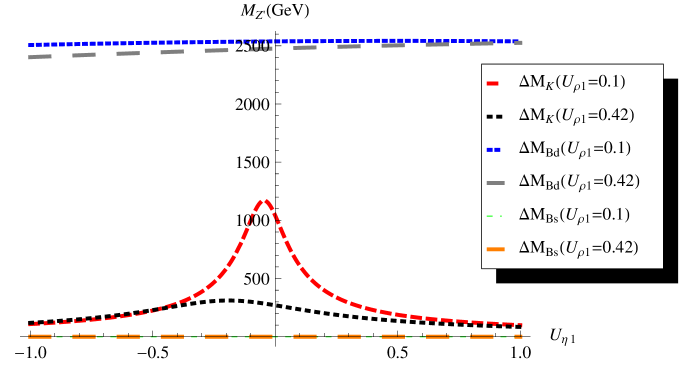
Figure 1: $Z^{\prime}$ mass values satisfying Eq. (66) and Eq. (78), simultaneously, but not including the pseudoscalar contribution, for a fixed value of the element $U_{\rho 1}$ ($U_{\eta 1}$), and the other $U_{\eta 1}$ ($U_{\rho 1}$) running in the range $[-1,1]$.

Fist, we will not consider in (66) the pseudoscalar $A^{0}_{1}$, assuming that $U_{\eta 1}$ and $U_{\rho 1}$ are real and within the interval $[-1,1]$. Next, we will keep $U_{\rho 1}$ fixed and varying $U_{\eta 1}$, we obtain the corresponding $Z^{\prime}$ mass which satisfies Eq. (66) that runs from GeVs to few TeVs. See the curves in Figs. 1-3 and discussion in Sec. VII.

In the next subsection we will consider FCNC processes as in the previous one but now involving the $b$ quark.

IV.2 $\Delta M_{B}$

We can also consider the $B^{0}_{d}-\bar{B}^{0}_{d}$ mass difference, $\Delta M^{SM}_{B}=\zeta^{SM}_{bd}\langle\bar{B}^{0}|(\bar{s}d)^{2}_{V-A}|B^{0}\rangle$ where $\langle\bar{B}^{0}|(\bar{b}d)^{2}_{V-A}|B^{0}\rangle=M_{B}f^{2}_{B}/3$ buras , and, as before, we factorized the model independent factors

$$\zeta^{SM}_{bd}=\frac{G^{2}_{F}M^{2}_{W}}{12\pi^{2}}\,S_{0}(x_{t})[(V_{CKM})^{*}_{td}(V_{CKM})_{tb}]^{2}\approx 1.0329\times 10^{-12}\,\textrm{GeV}^{-2},$$ (67)

where $x_{t}=m^{2}_{t}/M^{2}_{W}$ and we have used $S_{0}(x)\approx 0.784x_{t}^{0.76}$ schneider .

From Eqs. (28)-(31) the effective Hamiltonian contributing to the $B^{0}_{d}\leftrightarrow\bar{B}^{0}_{d}$ transition is given by

$$\mathcal{H}^{\Delta B=2}_{eff}|_{Z^{\prime}}=\frac{g^{2}}{4c^{2}_{W}M^{2}_{Z^{\prime}}}[\bar{b}_{L}(K^{D}_{L})_{bd}\gamma^{\mu}d_{L}]^{2},$$ (68)

and we obtain the following extra contributions to $\Delta M_{B_{d}}$, using here and below, appropriate matrix elements as in Eq. (60) for the kaon system,

$$\Delta M_{B_{d}}|_{Z^{\prime}}=2\textrm{Re}\,\langle\bar{B}^{0}|\mathcal{H}^{\Delta B=2}_{eff}|_{Z^{\prime}}|B^{0}\rangle=\textrm{Re}\,\zeta^{Z^{\prime}}_{bd}\,\langle\bar{B}^{0}|(\bar{b}d)^{2}_{V-A}|B^{0}\rangle$$ (69)

where, and we have not considered the QCD corrections and the bag parameter $B_{B}=1$. We obtain

$$\textrm{Re}\,\zeta^{Z^{\prime}}_{bd}=\textrm{Re}\,\frac{G_{F}}{2\sqrt{2}c^{2}_{W}}\,\frac{M^{2}_{W}}{M^{2}_{Z^{\prime}}}\;[(K^{D}_{L})_{bd}]^{2}\,=10^{-9}\,\frac{M^{2}_{W}}{M^{2}_{Z^{\prime}}}\,\textrm{GeV}^{-2},$$ (70)

where we have used (39), i.e., $(K^{D}_{L})_{bd}=-8.3\times 10^{-3}$.

Similarly we have the scalar contributions in the $B^{0}_{q}-\bar{B}^{0}_{q}$ system ($q=d,s$). From Eqs. (40) and (51) the scalar interactions between the $b$, $d$ quarks mediated by the scalars $h^{0}_{i}$ are given by

$$-\mathcal{L}_{bqh} = \frac{1}{\sqrt{2}}\sum_{i}[(I^{i}_{B_{d}})_{bq}\bar{b}_{L}d_{R}+(I^{\prime i}_{B_{d}})_{bq}\bar{d}_{L}b_{R}]h^{0}_{i}+H.c.$$ (71)

$$= \frac{1}{2\sqrt{2}}\sum_{i}[(I^{i+}_{B_{d}})_{bq}(\bar{b}d)+(I^{i-}_{B_{d}})_{bq}(\bar{b}\gamma_{5}d)]h^{0}_{i}+H.c.,$$

where $(I^{i}_{B_{d}})_{q_{1}q_{2}}=(\mathcal{K}^{D})_{q_{1}q_{2}}U_{\alpha i};\;\alpha=\eta,\rho;\;q_{i},q_{2}=b,d$. The respective entries of the matrix $\mathcal{K}^{D}$ can be obtained from Eq. (51). We have defined $(I^{i\pm}_{B})_{bq}=(I^{\prime i}_{B_{d}})_{bq}\pm(I^{i*}_{B_{d}})_{qb}$. For the case when $q=d$ we obtain

$$(I^{i}_{B_{d}})_{bd}\approx 10^{-6}U_{\rho i}-10^{-5}U_{\eta i},\,\,(I^{i}_{B_{d}})_{db}\approx-10^{-4}U_{\rho i}+10^{-5}U_{\eta i}.$$ (72)

The contributions of the pseudoscalar fields are similar to those of the scalar $h^{0}_{i}$ but making $h^{0}_{1}\to A^{0}_{i}$ in (71), and $U_{\eta i}\to V_{\eta i}$ and $U_{\rho i}\to V_{\rho i}$ in Eq. (72).

The effective Hamiltonian induced by (71), contributing to the $B^{0}_{d}\leftrightarrow\bar{B}^{0}_{d}$ transitions is:

$$\mathcal{H}^{\Delta B=2}_{eff}|_{h+A} = \sum_{i}\frac{1}{8m^{2}_{i}}[(I^{i+}_{B})^{2}_{bq}(\bar{b}q)^{2}+(I^{i-}_{B})^{2}_{bq}(\bar{b}\gamma_{5}q)^{2}]$$ (73)

$$- \sum_{i}\frac{1}{8m^{2}_{A}}[[(I^{i+}_{B})^{A}_{bq}]^{2}(\bar{b}q)^{2}+[(I^{i-}_{B})^{A}_{bq}]^{2}(\bar{b}\gamma_{5}q)^{2}].$$

and, as usual we define

$$\Delta M_{B_{d}}|_{h,A}=2\textrm{Re}\langle\bar{B}^{0}|\mathcal{H}^{\Delta B=2}_{eff}|_{h}|B^{0}\rangle=\textrm{Re}\zeta^{h}_{bd}\,\langle\bar{B}^{0}|(\bar{b}d)^{2}_{V-A}|B^{0}\rangle$$ (74)

where

$$\textrm{Re}\,\zeta^{h}_{bd}=\textrm{Re}\sum_{i}\frac{1}{32m^{2}_{i}}\left[0.6(I^{i+}_{B_{d}})^{2}_{bd}-16.5(I^{i-}_{B_{d}})^{2}_{bd}\right]\,\textrm{GeV}^{-2},$$ (75)

and

$$(I^{i\pm}_{B_{d}})^{2}_{bd}=[(U_{\rho i}-0.2U^{*}_{\eta i})U_{\rho i}\pm 0.2U_{\eta i}U_{\rho i}]\times 10^{-8},$$ (76)

then

$$\textrm{Re}\,\zeta^{h}_{bd}=\textrm{Re}\sum_{i}\frac{1}{32m_{i}^{2}}\{0.6((U_{\rho i}-0.2U^{*}_{\eta i})U_{\rho i}+0.2U_{\eta i}U_{\rho i}))$$

$$-16.5((U_{\rho i}-0.2U^{*}_{\eta i})U_{\rho i}-0.2U_{\eta i}U_{\rho i})\}\times 10^{-8}.$$ (77)

Assuming that only one of the scalars contribute in (61), we obtain a constraint on the contributions of $Z^{\prime}$, one scalar $h^{0}_{1}$ and one pseudoscalar $A^{0}_{1}$ to $\Delta M_{B}$, like that in Eq. (66) for the kaon system:

$$10^{-1}\,\frac{M^{2}_{W}}{M^{2}_{Z^{\prime}}}\,+\frac{1}{32m^{2}_{1}}\{0.6[(U_{\rho 1}-0.2U^{*}_{\eta 1})U_{\rho 1}+0.2U_{\eta 1}U_{\rho 1}]$$

$$-16.5[(U_{\rho 1}-0.2U^{*}_{\eta 1})U_{\rho 1}-0.2U_{\eta 1}U_{\rho 1}]-\mathcal{A}^{\prime}\}\,<10^{-4}\,\textrm{GeV}^{-2}.$$ (78)

where $\mathcal{A}^{\prime}$ is the pseudoscalar contribution which is also similar to that of the scalar one in (77) but with $m_{1}\to m_{A}$ and $U_{\eta 1}\to V_{\eta 1}$ and $U_{\rho 1}\to V_{\rho 1}$. The analysis of the $B_{s}-\bar{B}_{s}$ system follows the same procedure.

As can be seen from Figs. 1,2 and 4, the constraints coming from $B_{d}-\bar{B}_{d}$ are stronger than those in the $K^{0}-\bar{K}^{0}$ and $B_{s}-\bar{B}_{s}$. Moreover, in the $B_{d}$ system the interference of $Z^{\prime}$ with the pseudoscalar is what matters, although this is not as important as in the kaon system. See Sec. VII for discussions. We will see in the next section that the interference is more dramatic in the $\Delta M_{D}$ case.

V What Higgs boson is this?

We have assumed that the mass of the lightest scalar is equal to that of the resonance found at LHC cmsatlas . We see from Fig. 1 that the values of the $M_{Z^{\prime}}$ allowed by $\Delta F=2$ processes depend on $U_{\rho 1}$ and $U_{\eta 1}$ matrix elements in the neutral scalar sector. The other factor denoted by $\mathcal{\bar{K}}^{Ux}_{q_{1}q_{2}}$, have already been fixed. Assuming that the production processes are the same of the SM (new sources should be suppressed by the masses of the extra particles of the model), the neutral scalar $h^{0}_{1}$, must couple to fermions, at least to the top quark, with a similar strength to that in the SM, in order to have a compatible Higgs boson production rate. The latter point is important since the new resonance discovery at LHC cmsatlas is still compatible with the SM expectation and it has couplings to fermion and vector bosons compatible with the SM Higgs giardino . In $d$-type quark sector we have already seen that only the $b$-quark has a coupling to that resonance that can be smaller than the SM one.

From Eqs. (40) and (47), the $u$-type quark-neutral-scalar couplings are

$$\mathcal{K}^{U}\approx\left(\begin{array}[]{ccc}0.0099\rho^{0}-10^{-6}\eta^{0}&0.00340\rho^{0}-10^{-5}\eta^{0}&0.0109\rho^{0}-10^{-5}\eta^{0}\\ -0.13846\rho^{0}+10^{-7}\eta^{0}&0.0556\rho^{0}+10^{-6}\eta^{0}&-0.1521\rho^{0}-10^{-6}\eta^{0}\\ 1.9228\rho^{0}-10^{-11}\eta^{0}&0.8656\rho^{0}-10^{-10}\eta^{0}&2.3569\rho^{0}-10^{-10}\eta^{0}\end{array}\right).$$ (82)

V.1 $\Delta M_{D}$

Let us now consider a $\Delta C=2$ process: the mass difference between charmed neutral mesons, $\Delta M_{D}$. We use the numbers in Eqs. (39) and (82) for the transition $D^{0}\leftrightarrow\bar{D}^{0}$. $(K^{U}_{L})_{uc}\sim 8.9\times 10^{-2}$, and $(I^{1\pm})_{uc}=[0.0034\mp 0.138]U_{\rho 1}$, that is $(I^{1+})_{uc}=-0.057$ and $(I^{1-})_{uc}=0.06$. Hence, We obtain

$$\Delta M_{D}=\left(1.3\frac{M^{2}_{W}}{M^{2}_{Z^{\prime}}}-4.05\right)\times 10^{-9}\;\textrm{GeV},$$ (83)

and we see that $M_{Z^{\prime}}>43$ GeV gives agreement with the experimental value already, but with the $Z^{\prime}$ alone we would obtain $M_{Z^{\prime}}>27$ TeV.

V.2 Higgs-$u$-quark couplings

The Yukawa couplings in the SM are $y_{u}=1.3\times 10^{-5}$, $y_{c}=7.3\times 10^{-3}$ and $y_{t}=0.997$. In the present model these values correspond to the diagonal entries in the matrix (82). From the latter, we see that the couplings of the $u,c$-quarks are dominated by the neutral scalar $\rho^{0}$, and it may be compatible with the SM values depending of the values of $U_{\rho 1}$. From Eq. (82) we see that the larger coupling of $h^{0}_{1}$ is with the top quark and can be numerically equal to the coupling in the SM, if $U_{\rho 1}=0.42$ regardless the value of $U_{\eta 1}$, i.e., $(\mathcal{\bar{K}}^{U\rho})_{tt}U_{\rho 1}=\sqrt{2}m_{t}/v\sim 0.9974$. In this case we have that $(\mathcal{\bar{K}}^{U\rho})_{uu}U_{\rho 1}=0.0042$ and $(\mathcal{\bar{K}}^{U\rho})_{cc}U_{\rho 1}=0.0233$. These values are larger than the respective ones in the SM. However this is not a problem by now. With the present data it is not possible to measure $y_{c}$ directly.

Nevertheless this may not be the full history. In 3-3-1 models there are extra heavy quarks, and hence, the gluon fusion can produce the SM-like Higgs throughout new diagrams involving the extra quarks. These exotic quarks are singlet non-quiral quarks under the gauge symmetry of the SM. However, they are quiral quarks under the 3-3-1 symmetry and couple to the neutral scalar $\chi^{0}$, which is a singlet under the SM gauge symmetries and has a projection on the SM-like neutral scalar given by $U_{\chi 1}$. Hence, $gg\to h^{0}_{1}$ may have contributions from these exotic quarks that are proportional to $U^{2}_{\chi 1}$, but independent of the exotic quark masses, they would be smaller than $U_{\eta 1}$, and $U_{\rho 1}$ since the $\chi^{0}$ must have its main projection on a heavy neutral scalar. These parameters together can still mimic the SM Higgs production unless the exotic quarks are too heavy, or $U_{\chi 1}$ is very small, as we are assuming here. However, if the exotic quarks are not too heavy, or $U_{\chi 1}$ is larger than we thought, these quarks will contribute significantly to the $h^{0}_{1}$ production but, since at the same time the rates will be reduced, it is possible that some observables do not change. In the latter case we could consider $U_{\rho 1}$ again as a free parameter and the $h^{0}_{1}$ does not necessarily is the SM-like Higgs. It can be one of the extra Higgs in the model i.e., it is not the resonance that was discovered at LHC.

As we said before, the couplings of the 125 GeV Higgs boson to $W$, $Z$ and fermions may have strength that can be smaller than the respective couplings in the SM gupta since these couplings are modify by the matrix elements like $U_{\eta 1}$ and $U_{\rho 1}$. However, the Yukawa couplings, see as in Eqs. (51) and (82), may be larger or smaller than the SM couplings flavour . For instance, top quark decay $t\to c\,h^{0}_{1}$ is now possible, and written the respective couplings by $\bar{c}(a+i\gamma_{5}b)t$, we have from Eq. (78) that $a=[(\mathcal{K}^{U})_{ct}+(\mathcal{K}^{U})^{*}_{tc}](U_{\rho 1}/2)$ and $b=[(\mathcal{K}^{U})_{ct}-(\mathcal{K}^{U})^{*}_{tc}](U_{\rho 1}/2)$. Using the numerical values in Eq. (78) we see that $a\approx 0.15$ and $b\approx 0.21$. The value of $(a+b)/2\approx 0.18$ may be considered consistent with the recent upper limit for the coupling of the vertex $\bar{c}th^{0}_{1}$ obtained by the ATLAS: $a<0.17$ atlasnote . Having fixed the values of $U_{\rho 1}$ and allowing $U_{\eta 1}$ to run over the range $[-0.2,0.2]$ and the other numbers in Eq. (82) we do not have any freedom with the $\Delta M_{D}$ observable. In this case the interference between the neutral scalar and the $Z^{\prime}$ contributions are more dramatic: only the $Z^{\prime}$ implies $M_{Z^{\prime}}>27$ TeV and the scalar contributions alone give a large contribution: both, however, imply $M_{Z^{\prime}}>42.5$ GeV. Here we have not consider the pseudoscalar contributions to $\Delta M_{D}$. Once again we would like to emphasize that all of this is at $\mu=M_{Z}$.

In the next section we consider the $|\Delta F|=1$ forbidden processes.

VI $\Delta F=1$ processes

Concerning the $|\Delta F|=1,\;F=S,B$ processes, we consider as an illustration the leptonic decays of neutral mesons, $M^{0}$, i.e., $M^{0}\to l^{+}l^{\prime-}$, with $l,l^{\prime}=e,\mu$; and $M^{0}$ an strange or a beauty meson. We recall that these processes, at the tree level, involve only one vertex in the quark sector and the $Z^{\prime}$ has natural flavor conservation in the lepton sector. When a (pseudo)scalar is exchanged, the other vertex involves the interactions of the charged leptons that do not conserve the lepton flavor. This is parameterized by the arbitrary matrix $U_{ll^{\prime}}$ as discussed below.

In the m3-3-1 model the partial width of the decay $M^{0}(q_{1}\bar{q}_{2})\to l^{+}l^{\prime-}$, where $M^{0}=K,B_{d,s}$ has contributions at tree level which, are given by

$$\mathcal{B}^{331}_{M\to l^{+}l^{\prime-}}\! = \!\left\{\frac{G_{F}M^{2}_{W}}{16\sqrt{2}c^{2}_{W}}|(K^{D}_{L})_{q_{1}q_{2}}|^{2}\frac{f^{2}_{M}M^{2}_{M}m^{2}_{l}}{M^{4}_{Z^{\prime}}}\!+\!\frac{M^{6}_{M}f^{2}_{M}}{2(m_{q_{1}}\!+\!m_{q_{2}})^{2}}\left[\left|\frac{(I_{M})_{q_{1}q_{2}}U_{ll^{\prime}}}{m^{4}_{h_{1}}}\right|^{2}+\left|\frac{(I_{M})^{A}_{q_{1}q_{2}}U^{A}_{ll^{\prime}}}{m^{4}_{A}}\right|^{2}\right]\right.$$ (84)

$$- \!\left.\frac{(\sqrt{2}G_{F}M^{2}_{W})^{\frac{1}{2}}}{64c_{W}}\frac{M^{4}_{M}f^{2}_{M}m_{l}}{(m_{q_{1}}\!+\!m_{q_{2}})M^{2}_{Z^{\prime}}M^{2}_{h_{1}}}(K^{D}_{L})_{q_{1}q_{2}}(I_{M})^{*}_{q_{1}q_{2}}U^{*}_{ll^{\prime}}\right\}\frac{(1\!-\!\frac{4m^{2}_{l}}{M^{2}_{M}})^{\frac{3}{2}}\tau_{M}}{16\pi M_{M}},$$

where $\tau_{M}$ is the meson $M^{0}$ half-life, $M_{M}$ its mass and we have used the meson matrix elements

$$\langle 0|\bar{q}_{f}\gamma_{\mu}\gamma_{5}q_{i}|M^{0}\rangle=if_{M}p^{\mu}_{M},\quad\langle 0|\bar{q}_{f}\gamma_{5}q_{i}|M^{0}\rangle=-if_{M}\,\frac{M^{2}_{M}}{m_{q_{f}}+m_{q_{i}}},$$ (85)

and $p_{M}=p_{1}+p_{2}$.

The matrix $U_{ll^{\prime}}$ in (84) arises as follows. The three lepton generations transform under the 3-3-1 symmetry as $\Psi_{a}=(\nu_{a}\,l_{a}\,l^{c})^{T}_{L}\sim(1,\textbf{3},0)$ and we do not introduce right-handed neutrinos. The Yukawa interactions in the lepton sector are:

$$-\mathcal{L}_{\nu lH}=\epsilon_{ijk}\overline{(\Psi_{ia})^{c}}G^{\eta}_{ab}\Psi_{jb}\eta_{k}+\overline{(\Psi_{ia})^{c}}G^{S}_{ab}\Psi_{jb}S^{*}_{jk}+H.c.,$$ (86)

where $a,b$ are generations indices, $i,j,k$ are $SU(3)$ indices, and $G^{\eta}$ ($G^{S})$ is a antisymmetric (symmetric) matrix. In Eq. (86), $\eta$ is the same triplet which couples to quarks and $S$ is a sextet, $S\sim(1,\textbf{6},0)$ which does not couple to quarks. Under $SU(2)_{L}\otimes U(1)_{Y}$ the sextet transform as $S=\textbf{1}+\textbf{2}+\textbf{3}$, and we see that there is a doublet and a non-Hermitian triplet which gives mass to charged leptons and active left-handed neutrinos, respectively. However, although the sextet is enough to give to neutrinos a Majorana mass and a Dirac mass to the charged leptons, it does not give a $PMNS$ matrix $V_{PMNS}=U^{l\dagger}_{L}U^{\nu}_{L}$, since when only the sextet is the source of lepton masses we have that $U^{l}_{L}=U^{\nu}$. Hence the interaction with the $\eta$ triplet is mandatory. In this case the mass matrices of the neutrinos and charge leptons are

$$-\mathcal{L}^{\nu}_{M}=\overline{(\nu_{aL})^{c}}G^{S}_{ab}\nu_{bL}\frac{v_{\sigma_{1}}}{\sqrt{2}}+H.c.,\quad\mathcal{L}^{l}_{M}=\bar{l}_{iaL}\left[G^{\eta}_{ab}\frac{v_{\eta}}{\sqrt{2}}+G^{S}_{ab}\frac{v_{\sigma_{2}}}{\sqrt{2}}\right]l_{jbR}+H.c.,$$ (87)

where $\sigma^{0}_{1}$ and $\sigma^{0}_{2}$ are the neutral component of the triplet and doublet in the sextet, respectively. In terms of the mass eigenstates we have $Re\,\sigma^{0}_{1}=\sum_{i}U_{Si}h^{0}_{i}$, $Re\,\sigma^{0}_{2}=\sum_{i}U_{Di}h^{0}_{i}$, $Im\,\sigma^{0}_{1}=\sum_{i}V_{Si}h^{0}_{i}$ and $Im\,\sigma^{0}_{2}=\sum_{i}V_{Di}h^{0}_{i}$.

We have $M^{\nu}_{ab}=G^{S}_{ab}\frac{v_{\sigma_{1}}}{\sqrt{2}}$ and $M^{l}_{ab}=G^{\eta}_{ab}\frac{v_{\eta}}{\sqrt{2}}+G^{S}_{ab}\frac{v_{\sigma_{2}}}{\sqrt{2}}$. These mass matrices are diagonalized as follows: $\hat{M}^{\nu}=U^{\nu T}_{L}M^{\nu}U^{\nu}_{L}$ and $\hat{M}^{l}=U^{l}_{L}M^{l}U^{\dagger}_{R}$ and the relation between symmetry eigenstates (primed) and mass (unprimed) fields are $l^{\prime}_{L,R}=U^{l}_{L,R}l_{L,R}$ and $\nu^{\prime}_{L}=U^{\nu}_{L}\nu_{L}$, where $l^{\prime}_{L,R}=(e^{\prime},\mu^{\prime},\tau^{\prime})^{T}_{L,R}$, $l_{L,R}=(e,\mu,\tau)^{T}_{L,R}$ and $\nu^{\prime}_{L}=(\nu_{e}\,\nu_{\mu}\,\nu_{\tau})^{T}_{L}$ and $\nu_{L}=(\nu_{1}\,\nu_{2}\,\nu_{3})_{L}$.

The interactions of the neutral scalars and pseudo-scalars with the leptons are

$$-\mathcal{L}_{leptons} = \sum_{i,n=1,2,3}\overline{(\nu_{nL})^{c}}\nu_{nL}\frac{\sqrt{2}m_{\nu_{n}}}{v_{\sigma_{1}}}(U_{Si}h^{0}_{i}+iV_{Si}A^{0}_{i})$$ (88)

$$+ \sum_{i,l,l^{\prime}}\bar{l}_{L}U^{l\dagger}_{L}\{[G^{\eta}_{ll^{\prime}}U_{\eta i}+G^{S}_{ll^{\prime}}U_{Si}]h^{0}_{i}+i[G^{\eta}_{ll^{\prime}}V_{\eta i}+G^{S}_{ll^{\prime}}V_{Di}]A^{0}_{i})\}U^{l}_{R}l^{\prime}_{R}+H.c.$$

where $l,l^{\prime}=e,\mu,\tau$. For one scalar $h^{0}_{1}$ and one pseudoscalar $A^{0}_{1}$ we have

$$U_{ll^{\prime}}=U^{l\dagger}_{L}[G^{\eta}_{ll^{\prime}}U_{\eta 1}+G^{S}_{ll^{\prime}}U_{D1}]U^{l}_{R},\quad U^{A}_{ll^{\prime}}=U^{l\dagger}_{L}[G^{\eta}_{ll^{\prime}}V_{\eta 1}+G^{S}_{ll^{\prime}}V_{D1}]U^{l}_{R},$$ (89)

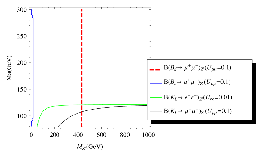
Figure 11: Considering the meson semi-leptonic decays including now the contribution of the pseudo scalar, the allowed region for the $Z^{\prime}$ and the pseudoscalar $A^{0}_{1}$ masses, for a fixed value of $U_{\eta 1}=V_{\eta 1}=0.1$ and $U_{\rho 1}=V_{\rho 1}=0.42$. The allowed region is always to the right and bounded by the curves and the biggest constrain came from $K_{L}\rightarrow\mu^{+}\mu^{-}$.

respectively. To be consistent with our previous analysis $U_{D1}$ and $V_{D1}$ have to be smaller than the other entries of the $U$ and $V$ matrices and can be neglected. It is the arbitrary matrix in Eq. (89) which appears in Eq. (84). Notice that it is sum of two products involving four matrices each. The FCNC effects in the charged lepton sector can be avoided only by fine tuning as $G^{\eta}_{e\mu}\frac{v_{\eta}}{2}+G^{S}_{e\mu}\frac{v_{\sigma_{2}}}{2}=0$, etc. Otherwise, we have processes like $l\to l^{\prime}\gamma$, $l\to\bar{l}^{\prime}l^{\prime}l^{\prime\prime}$ , where $l=\mu,\tau$ and $l^{\prime},l^{\prime\prime}=e,\mu$. For instance, experimentally it is found $\mathcal{B}_{\mu\to e+\gamma}<5.7\times 10^{-13}$ meg , a value still well above the SM prediction $\sim 10^{-52}$ cheng . In the present model this decay occurs at the 1-loop level too. On the other hand decays like $\mu^{+}\to e^{+}e^{-}e^{+}$. with branching ratio $<10^{12}$ sindrum occurs at the tree level mediated by neutral scalars, in particular by the $h^{0}_{1}$. The branching ratio of this decay in the m3-3-1 model is proportional to $(1/G^{2}_{F}m^{4}_{1})|U_{ee}U_{e\mu}|^{2}\sim 3\times 10^{-3}|U_{e\mu}|^{2}$ and constrains mainly the non-diagonal matrix element $U_{e\mu}$ which we recall is the arbitrary matrix defined in Eq. (89). Since $U_{ee}<10^{-2}$ with the larger values corresponding to the case when we consider also the pseudoscalar (see Fig. 11), we have that $|U_{e\mu}|^{2}<10^{-5}$. We can see from the definition of the $U$ matrix in Eq. (89) that it is not a too-strong constraint since this matrix is the sum of the two products of four matrices with two of them being ($G^{\eta},G^{S}$) arbitrary ones. Decays like $h^{0}_{1}\to\mu^{+}\tau^{-}$ can be observable at the LHC blankenburg . More details on this will appear elsewhere.

It worth to call to the attention that the m3-3-1 does not need the introduction of singlet right-handed neutrinos for having massive (light) active Majorana neutrinos and also accommodated the PMNS mixing matrix. If we add right-handed neutrinos and avoid, by an appropriate symmetry, the coupling of $\eta$ to leptons we have $M^{\nu}_{ab}=G^{\eta}_{ab}\frac{v_{\eta}}{\sqrt{2}}+G^{S}_{ab}\frac{v_{\sigma_{1}}}{\sqrt{2}}$ and $M^{l}_{ab}=G^{S}_{ab}\frac{v_{\sigma_{2}}}{\sqrt{2}}$ and the FCNC arise in the neutrino sector. I n the most general case FCNC occur in both sectors. The 3-3-1 model with right-handed neutrinos transforming non-trivially under $SU(3)_{L}$ was first put forward by Montero et al., in Ref. mpp . Anyway, if sterile right-handed neutrinos (with respect to the SM interactions) do exist, they can be accommodated in an $SU(4)_{L}\otimes U(1)_{X^{\prime}}$ model, see Ref. pp94 . Summarizing, the m3-3-1 model ought to have FCNC in the scalar-charged lepton interactions if no right-handed neutrinos (transforming as singlets under $SU(3)_{L}$) are added to the matter content of the model.

Now, we are able to discuss leptonic decay of neutral mesons.

VI.1 $K_{L}\to l^{+}l^{-}$

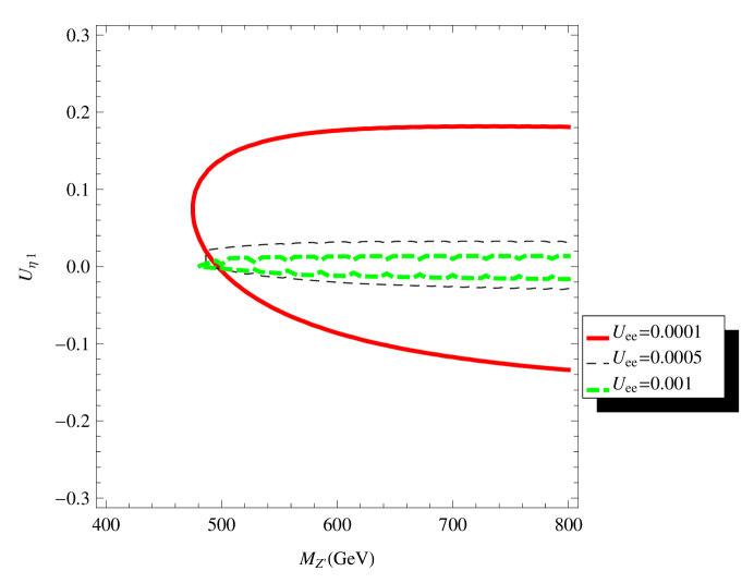
Figure 6: Same as Fig. 5 but now showing the dependence on $U_{ee}$. The red (continuos) line is with $U_{ee}=10^{-4}$, $U_{ee}=5\times 10^{-4}$ black (thin dashed) line and $U_{ee}=10^{-3}$ green (thick green) line. The allowed region is always to the right and bounded by the curves.

The experimental data are $\mathcal{B}_{K_{L}\to e^{+}e^{-}}<10^{-12}$ and $\mathcal{B}_{K_{L}\to\mu^{+}\mu^{-}}=(6.84\pm 0.11)\times 10^{-9}$ pdg . Using $q_{1}=s$ and $q_{2}=d$, $M_{M}=M_{K}$, $f_{M}=f_{K}$, we obtain from Eq. (84) that the decay into electrons imposes a strong bond on the values of $U_{\eta 1}$ but not on $M_{Z^{\prime}}$. This is shown in Figs. 5 for $K_{L}\to e^{+}e^{-}$ decay. We have an additional free parameter, $U_{ee}$, that weakens this bonds, see Fig. 6. For the $K_{L}\to\mu^{+}\mu^{-}$ decay see Fig. 7. On the other hand, the bound from the two muon decay on the $Z^{\prime}$ mass it is less restrictive than $K_{L}\to e^{+}e^{-}$. See also the discussion in Sec. VII.

VI.2 $B_{s,d}\to\mu^{+}\mu^{-}$

Next we consider $\Delta B=1$ processes. Recently, it has been observed the branching ratio $\mathcal{B}_{B^{0}_{s}\to\mu^{+}\mu^{-}}=3.2\times 10^{-9}$ and $\mathcal{B}_{B^{0}_{d}\to\mu^{+}\mu^{-}}=8\times 10^{-10}$ lhcb . In Both cases there is not constraint in $U_{\mu\mu}$, however, $U_{\eta 1}$ has the biggest constraint from the $\mathcal{B}_{B^{0}_{d}\to\mu^{+}\mu^{-}}$ decay, as can be seen in Fig. 8 (the solid gray curve), being the allowed interval around $[-0.5,0.5]$. The constraint on $M_{Z^{\prime}}$, for both cases, is weaker than those coming from the other processes. In fact, these decays allow a rather light $Z^{\prime}$ as is shown in Fig. 9. In the latter figure we show also the constraint coming from the $K_{L}$ decays and $\Delta M_{K}$.

VII Results

Here we will discuss in more details the constraints on the $Z^{\prime}$ mass taking into account both the scalar and pseudoscalar contributions to the processes discussed above. First, let us consider the $\Delta M_{M},\;M=K,B_{d,s}$ cases. In each case we first consider only the scalar $h^{0}_{1}$ contribution by considering the pseudoscalar very heavy ($m_{A}\to\infty$), in practice we have used $m_{A}=100$ TeV when we want to decouple the pseudoscalar $A^{0}_{1}$ from Eqs. (66), (78) and (84). For the sake of simplicity we consider that the mixing matrix elements in the scalar and pseudoscalar sector have the same numerical values, i..e, $U_{\eta 1}=V_{\eta 1}$ and $U_{\rho 1}=V_{\rho 1}$. We are also assuming that the other scalars and pseudoscalars in the model, even if their projections on $h^{0}_{1},A^{0}_{1}$ are large, are heavy enough to give no observable effects in the processes considered above. It implies that even if we use $U_{\rho 1}=V_{\rho 1}=0.42$, $U_{\eta 1}$ and $V_{\eta 1}$ are still free parameters but we will consider them to be equal, i..e, $U_{\eta 1}=V_{\eta 1}$, just for simplicity. We would like to recall that all our results are consequences of the mixing matrices $V^{U,D}_{L,R}$ obtained in Sec. II.

The scalar contribution (when the pseudoscalar is considered too heavy) to the $\Delta M_{M}$ mass differences are shown in Fig. 1. In this figure we show the values of $M_{Z^{\prime}}$, as a function of $U_{\rho 1}$ ($U_{\eta 1}$) for fixed $U_{\eta 1}$ ($U_{\rho 1}$), which are allowed by solving simultaneously Eqs. (66) and (78). In principle, both $U_{\rho 1}$ and $U_{\eta 1}$ are allowed to vary in the interval $(-1,1)$. We see from this figure that a large range for the $Z^{\prime}$ mass values is allowed by $K$-mesons but not by the $B_{s}$ and $B_{d}$ mesons. Notice also that under our conditions in Sec. II, $\Delta M_{B_{s}}$ does not constrain $m_{Z^{\prime}}$ at all. However, $\Delta M_{B_{d}}$ does: $m_{Z^{\prime}}>2.5$ TeV. On the other hand, by demanding that $\rho^{0}$ be equivalent to the SM Higgs implies, from Eq. (82), $U_{\rho 1}=0.42$, see Sec. V. In this case, the only variable is $U_{\eta 1}$, and the $Z^{\prime}$ mass can still be of the order of the electroweak scale or even lower. Fig. 2 shown the same as Fig. 1 but now with $U_{\rho 1}=0.42$. There is negative interference in the $K$ mesons system between the $Z^{\prime}$ and $h^{0}_{1}$ amplitudes: without the scalar contribution $\Delta M_{K}$ implies also $m_{Z^{\prime}}>2.5$ TeV. In the $B_{d,s}$ systems the interference is not important. If we allow the $A^{0}_{1}$’s mass to be a free parameter, we show in Figs. 3 and 4 the effects of this pseudoscalar in the $K$ and $B_{d,s}$ systems. Those figures show the allowed values for the masses $m_{A}$ and $m_{Z^{\prime}}$. For obtaining Figs. 3 and 4 we have assumed that $U_{\eta 1}=V_{\eta 1}$ and $U_{\rho 1}=V_{\rho 1}=0.42$. Notice that now there is negative interference between $Z^{\prime}$ and the pseudoscalar, $A^{0}_{1}$, implying a smaller lower bound on $m_{Z^{\prime}}$ in the $B_{d}$ system: $m_{Z^{\prime}}>2.3$ TeV. In the case os the $B_{s}$ system the scalar and pseudoscalar are not important and the constraint on the $Z^{\prime}$ mass is weaker than in the other mesons.

From Fig. 5 we see that in the case of $K_{L}\to e^{+}e^{-}$ decay, the interference between $Z^{\prime}$ and $h^{0}_{1}$ is constructive, assuming the contribution of the $A^{0}_{1}$ negligible. We use Eq. (84) with $l=l^{\prime}=e$ and $M^{0}=K$. The value of the $M_{Z^{\prime}}$ mass change, from 440 GeV when only the $Z^{\prime}$ contribution is consider, to 460 GeV when both the $Z^{\prime}$ and $h^{0}_{1}$ contribution are taken into account. The pseudoscalar contribution is omitted in this figure. The figure shows the allowed values for $M_{Z^{\prime}}$ and $U_{\eta 1}$, for fixed $U_{ee}=10^{-4}$, see Eq. (89), by this decay. The red (dashed) vertical line is the contribution of $Z^{\prime}$ only and the allowed range is to the right of the curve. The minimal value allowed by this decay is around 445 GeV. The blue (dashed) horizontal lines are the contributions of the scalar only and the allowed range for $U_{\eta 1}$, i.e., $-0.2<U_{\eta 1}<0.2$ for any value of $M_{Z^{\prime}}$. The total contribution is given by the green (continuous) curve and the allowed region is inside that curve, and the minimal value for $M_{Z^{\prime}}$ has moved to 500 GeV. Fig. 6 shows the total contribution (the green curve in Fig. 5) for several values of $U_{ee}$. Notice that $U_{\eta 1}$ is constrained, $|U_{\eta 1}|<0.2$.

For the decay $K_{L}\to\mu\mu$ we use Eq. (84) with $l=l^{\prime}=\mu$ and $M=K$. In Fig. 7, as in Fig. 5, the red (solid) vertical line is the contribution of the $Z^{\prime}$ only and the lower bound on the $Z^{\prime}$ mass is around 705 GeV. As can be seen from Fig. 8, the scalar contribution does not constrain $U_{\eta 1}$. The total contribution is given by the blue (dashed) curved line and $M_{Z^{\prime}}>740$ GeV. Notice from Fig. 7 that this decay has a destructively interference for $0.01<U_{\eta 1}<0.1$ and constructive for $U_{\eta 1}$ outside this region. Finally, see from Fig. 8 that the decay $B_{s}\to\mu\mu$ does not constrain these parameters anymore. In Fig. 9 we summarize all constraint when only $Z^{\prime}$ and $h^{0}_{1}$ are considered.

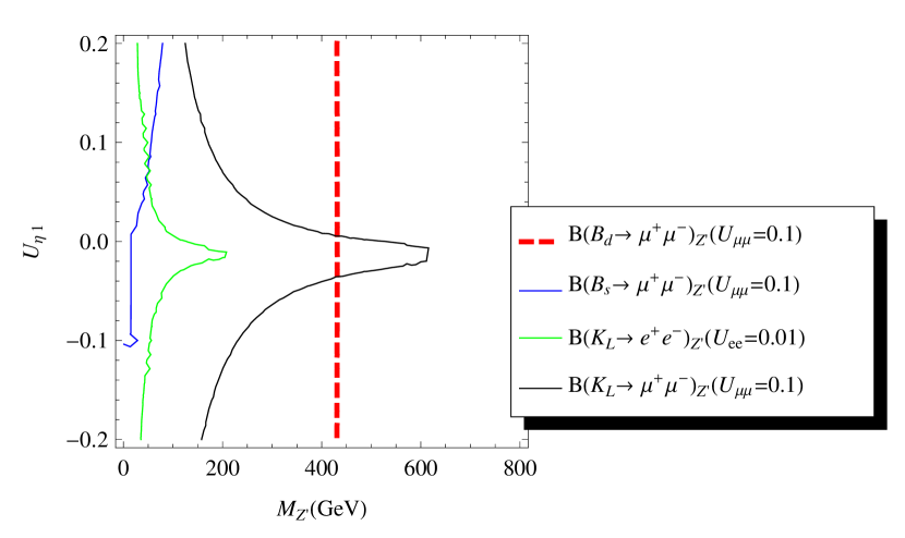
Figure 10: Here we consider the contribution of the pseudoscalar to the semi-leptonic decays. We are assuming that $U_{\eta 1}=V_{\eta 1}$ and $U_{\rho 1}=V_{\rho 1}$ which implies $U_{ee}=U^{A}_{ee}$ and $U_{\mu\mu}=U^{A}_{\mu\mu}$ in Eq. (84). The allowed region for the $Z^{\prime}$ mass and $U_{\eta 1}$ for fixed values to the pseudo scalar mass at $m_{A}=80$ GeV. The allowed region is always to the right and bounded by the curves and the biggest constraint comes from $K_{L}\to\mu^{+}\mu^{-}$.

The pseudoscalar effects in the leptonic meson decays are shown in Figs. 10 and 11 under the assumption that $U_{ll^{\prime}}=U^{A}_{ll^{\prime}}$ in Eq. (84), i.e., that $V_{\eta 1}=U_{\eta 1}$ and $V_{\rho 1}=U_{\rho 1}=0.42$ in Eq. (89). From the latter equation we see that this is not the more general case but we used it just for the sake of simplicity.

When the nontrivial SM limit discussed in Sec. III is satisfied, $Z$ and $Z^{\prime}$ decouple i.e., the respective mixing angle, say $\theta$, is zero at the tree level. In this case, the masses of the neutral vector bosons are given by

$$M^{2}_{1}=\frac{g^{2}}{4c^{2}_{W}}v^{2}_{W}\equiv M^{2}_{Z},\quad M^{2}_{2}=\frac{g^{2}}{2c^{2}_{W}}\frac{(1-2s^{2}_{W})(4+\bar{v}^{2}_{W})+s^{4}_{W}(4-\bar{v}^{4}_{W})}{1-4s^{2}_{W}}v^{2}_{\chi}\equiv M^{2}_{Z^{\prime}},$$ (90)

where $v^{2}_{W}=v^{2}_{\eta}+v^{2}_{\rho}+2v^{2}_{S}$, $\bar{v}_{W}=v_{W}/v_{\chi}$, and $v_{S}$ is the VEV of the sextet that we can neglect here. A lower limit of 2.3 TeV for $M_{Z^{\prime}}$ implies $v_{\chi}>1.6$ TeV, from Eq. (90). On the other hand, since the mass of the charged vector bosons, $W^{\pm}_{\mu},V^{\pm}_{\mu},U^{\pm\pm}_{\mu}$, are given by

$$M^{2}_{W}=\frac{g^{2}}{4}v^{2}_{W},\quad M^{2}_{V}=\frac{g^{2}}{4}(v^{2}_{\eta}+2v^{2}_{S}+v^{2}_{\chi}),\quad M^{2}_{U}=\frac{g^{2}}{4}(v^{2}_{\rho}+2v^{2}_{S}+v^{2}_{\chi}),$$ (91)

with $v_{\chi}>1.6$ TeV we have $M_{V}>532$ GeV and $M_{U}>527$ GeV, using $g^{2}=4\pi\alpha(Z)$. These values satisfy the upper bound newp

$$\frac{\sqrt{M^{2}_{V}-M^{2}_{U}}}{M_{W}}\leq\sqrt{3}\tan\theta_{W},$$ (92)

and not $M_{V}=M_{U}$, as is the case when we assume $v_{\chi}\gg v_{\eta},v_{\rho}$ from the very start. Notice that the exotic charged quarks, which masses are of the form $m_{j}=g_{j}v_{\chi}/\sqrt{2}$, may have masses of the order of 200-300 GeV for reasonable values of the dimensionless Yukawa couplings $g_{j}$.

VIII Conclusions

Here we have considered constraints coming from FCNC processes, $\Delta M_{K,B,D},K_{L}\to ee,\mu\mu$ and $B_{d,s}\to\mu\mu$, on the mass of the $Z^{\prime}$ neutral vector boson in the m3-3-1 model, taken into account, besides the $Z^{\prime}$, the contributions of the lightest scalar field, $h^{0}_{1}$, which we assume having a mass of 125 GeV, and a pseudoscalar with arbitrary mass, $m_{A}$. We first calculated all entries of the $V^{U,D}_{L,R}$ matrices which modified the Yukawa couplings in the quarks sector. Next, the matrix elements that relate the symmetry and mass eigenstates in the (pseudo)scalar sector, ($V_{\eta 1},V_{\rho 1}$) $U_{\eta 1},U_{\rho 1}$, are fixed by imposing the agreement with the measured mass differences and branching ratios, on the assumption that $V_{\eta 1}=U_{\eta 1}$ and $V_{\rho 1}=U_{\rho 1}$. We also have assumed that, the couplings of the scalar $h^{0}_{1}$ to the top quark were numerically equal to the coupling of the Higgs and the top quark in the SM and that the production mechanism was, for all practical purposes, the same of the Higgs of the SM as it was discussed in Sec. V. In most multi-Higgs models the couplings of $h^{0}_{1}$ to other fermions and to $W$ and $Z$ are not all full strength (i.e., the SM ones) because of the mixing among all the scalar fields (for an exception see Ref. flavour ). In the present model, some of these couplings may be larger and other smaller than the respective SM values, at least at $\mu=M_{Z}$.

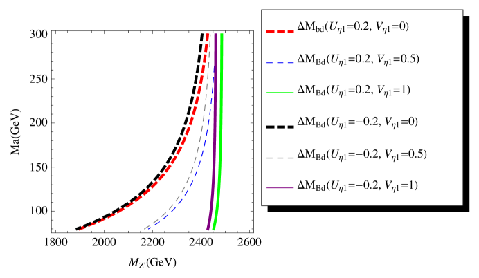
Figure 12: Same as Fig. 4 but now considering $V_{\eta 1}$ and $V_{\rho 1}$ independently of $V_{\eta 1}$ and $V_{\rho 1}$. Notice that the lower limit is smaller than in Fig. 4.

The amplitude of some of the neutral scalars interfere some times destructively, as in $\Delta M_{K,D}$, and some times constructively, as in the $K_{L}\to ll$ decay. If only $Z^{\prime}$ is considered, the lower bound on $M_{Z^{\prime}}$ from $\Delta M_{K}$ is $M_{Z^{\prime}}>2.5$ TeV and $>27$ TeV in $\Delta M_{D}$. When the neutral scalar is considered as well, the constraint is weaker allowing a rather light $Z^{\prime}$, see Secs. IV.1, IV.2 and V.1. The strongest constraint on the $Z^{\prime}$ mass comes from $\Delta B_{d}$, which is insensible to the scalar contributions and implies $m_{Z^{\prime}}>2.5$ TeV, but when one pseudoscalar is considered it becomes $m_{Z^{\prime}}>2.3$ TeV if the the pseudoscalar has a mass of around 180 GeV and under the conditions defined above. However, the latter upper limit depends on the conditions $V_{\eta 1}=U_{\eta 1}$ and $V_{\rho 1}=U_{\rho 1}$. If this is not the case, i.e., if $V_{\eta 1}$ and $V_{\rho 1}$ are considered free parameters, a smaller bound on the $Z^{\prime}$ mass is obtained: $M_{Z^{\prime}}>1.8$ TeV as can be seen in Fig. 12, which implies $v_{\chi}>1.27$ TeV, $M_{V}>412$ GeV, and $M_{U}>419$ GeV. The leptonic kaon decay into two leptons implies a lower bound for this mass of 740 GeV, see Sec VI for discussions.

A final remark is in order here. From Eqs. (40), (51) and (82), we see that the constraints depend on the matrix elements of $V^{q}_{L,R}$ given in Eqs. (18) and (27). These matrices have to diagonalize the quark mass matrices and hence they depend on the input parameters $G,G,\tilde{G},\tilde{F}$ and VEVs, in these mass matrices In this work we found a set of parameters that is compatible with the quark masses, at $\mu=M_{Z}$, and the CKM matrix. There could exist a different set, i.e., a different quark mass matrix, showing the same compatibility, which will be diagonalized by different $V^{q}_{L,R}$ matrices and, therefore, resulting in different values for the $Z^{\prime}$ mass constraint. The set we found is show below Eq.(27). We tried to find a different one without success. It seems that finding another set is not a trivial task, but it can, in principle, exist. There may be solutions with a heavy $Z^{\prime}$ when there is no destructive interference in the $\Delta M_{K}$ amplitude but there is in $\Delta M_{B_{d}}$, and so on. The main result of our work is shown that the interference between $Z^{\prime}$ and (pseudo)scalar fields exist in some range of the parameters. Hence, the effects considered here may be at work in $Z^{\prime}$-searches at the LHC as well but the interference will be with heavy (pseudo)scalars, different from $h^{0}_{1}$.

It is well known that the magnetic dipole transitions $b\to s+\gamma$, or $b\to d+\gamma$, have branching ratios of the order of $10^{-4}$ and are in agreement with the SM predictions babar . For a recent analysis see Ref. promberger2 . In the present model this sort of decays and CP violation also arise at the one-loop order through penguin and box diagrams. However, in the present case there are contributions of the singly and doubly charged scalars, exotic quarks, and singly and doubly charged vector bosons present in the model. The same happen with the $\Delta F=2$ processes since there are box diagrams involving singly and doubly charged scalar and vector bosons and exotic quarks as well. These contributions to $|\Delta F|=1,2$ will be considered elsewhere.

The search for a $Z^{\prime}$-like resonance has been done at the LHC. However, as in previous searches, the results are usually obtained in the context of a given model. For instance, in a top color assisted spontaneous symmetry breaking scenario this sort of (leptophobic) resonance has been excluded for $M_{Z^{\prime}}<1.3$ TeV, if $\Gamma_{Z^{\prime}}=0.012M_{Z^{\prime}}$, and $M_{Z^{\prime}}<1.9$ TeV, if $\Gamma_{Z^{\prime}}=0.10M_{Z^{\prime}}$ zprimecms . Notwithstanding, the application of these bounds to the model considered here is not straightforward and has to be done in a separate work.

Last but not least, we would like to say that the m3-3-1 solution that we have presented here can be falsifiable in the near future: When the strength of the $VVh^{0}_{1},\;V=W,Z$ where measured, given at least upper limits for $U_{\eta 1}$ and $U_{\rho 1}$, then we can check if all the couplings of the 125 GeV Higgs boson with the gauge bosons and all the fermions, when measured with sufficient precision, agree or not with those in Eqs. (51) and (82) when $\eta^{0}$ and $\rho^{0}$ are projected on $h^{0}_{1}$.

Figure 2: Same as Fig. 1 but now with $U_{\rho 1}=0.42$ (the value that ensures that the coupling of $h_{1}^{0}$ with the top quark is equal to the SM), and $U_{\eta 1}$ running in the interval $[-1,1]$.

Figure 3: Considering Eq. (66) with the contribution of the pseudoscalar. The allowed region for the $Z^{\prime}$ mass and the pseudoscalar mass $M_{a}$ were obtained by setting values for $U_{\eta 1}=V_{\eta 1}$. The smallest value to the $Z^{\prime}$ mass is when $U_{\eta 1}=V_{\eta 1}=0.2$ and the biggest when $U_{\eta 1}=V_{\eta 1}=-0.2$.

Figure 4: Considering the Eq. (78) with the contributions of the pseudoscalar. The allowed region for the $Z^{\prime}$ mass and the pseudoscalar mass $M_{a}$ were obtained by setting values for $U_{\eta 1}=V_{\eta 1}$. The smallest value to the $Z^{\prime}$ mass is when $U_{\eta 1}=V_{\eta 1}=-0.2$ and the biggest when $U_{\eta 1}=V_{\eta 1}=0.2$.

Figure 5: Allowed region for $M_{Z^{\prime}}$ and $U_{\eta 1}$, for fixed $U_{ee}=10^{-4}$ by the $K_{L}\to ee$ decay, using the Eq. (84), with $l=l^{\prime}=e$ and $M=K$). The red (dashed) vertical line is the contribution of $Z^{\prime}$ only, and the allowed range is to the right of the curve. The region within the blue (dashed) horizontal lines is the allowed region for the scalar contribution only. The total contribution is given by the green (continuous) curve and the allowed region is the area within this curve. Notice that we are not considering the pseudoscalar yet.

Figure 7: Constraints on $M_{Z^{\prime}}$ and $U_{\eta 1}$ from the $K_{L}\to\mu\mu$ decay fixed $U_{\mu\mu}=0.01$, using Eq. (84) with $l=l^{\prime}=\mu$ and $M=K$. The allowed regions are those to the right of the curves, for $M_{Z^{\prime}}$ and $U_{\eta 1}$. The red (solid) vertical line is the contributions of the $Z^{\prime}$ only. The blue (dashed) curved line is the total contribution to the decay. We consider only the $Z^{\prime}$ and the scalar contributions.

Figure 8: Same as Fig. 7 but now for $B_{d}\rightarrow\mu^{+}\mu^{-}$ and $B_{s}\rightarrow\mu^{+}\mu^{-}$ decays.

Figure 9: This figure summarizes all the previous results for $K^{0}-\bar{K}^{0}$, $B^{0}-\bar{B}^{0}$ mass differences and the $K^{0}$, $B_{s}$ and $B_{d}$ decays.

- (1) F. Pisano and V. Pleitez, Phys. Rev. D 46, 410, (1992); P. H. Frampton, Phys. Rev. Lett. 69, 2889, (1992); R. Foot, O. F. Hernandez, F. Pisano, and V. Pleitez, Phys. Rev. D 47, 4158, (1993).
- (2) V. Pleitez and M. D. Tonasse, Phys. Rev. D 48, 2353 (1993).
- (3) J. C. Montero, F. Pisano, and V. Pleitez, Phys. Rev. D 47, 2918 (1993); R. Foot, H. N. Long and T. A. Tran, Phys. Rev. D 50, R34 (1994); H. N. Long, Phys. Rev. D 53, 437 (1996).
- (4) A. G. Dias, R. Martinez, and V. Pleitez, Eur. Phys. J. C39, 101 (2005).
- (5) A. G. Dias and V. Pleitez, Phys. Rev. D80, 056007 (2009).
- (6) C. A. de S. Pires and O. P. Ravinez, Phys. Rev. D 58, 035008 (1998)
- (7) P.V. Dong, and H. N. Long, Int. J. Mod. Phys. A21, 6677 (2006), hep-ph/0507155.
- (8) P. B. Pal, Phys. Rev. D 52, 1659, (1995); A. G. Dias and V. Pleitez, Phys. Rev. D 69, 077702 (2004).
- (9) J. C. Montero, C. C. Nishi, V. Pleitez, O. Ravinez, and M. C. Rodriguez, Phys. Rev. D 73, 016003 (2006).
- (10) B. Dion, T. Gregoire, D. London, L. Marleau and H. Nadeau, Phys. Rev. D 59, 075006 (1999).
- (11) A. Alves, E. Ramirez Barreto, A. G. Dias, C.A.de S. Pires, F. S. Queiroz, P.S. Rodrigues da Silva, Phys.Rev. D84, 115004 (2011).
- (12) J. T. Liu, Phys. Rev. D 50, 542 (1994).
- (13) J. T. Liu and D. Ng, Phys. Rev. D 50, 548 (1994).
- (14) P. Jain and S. D. Joglekar, Phys. Lett. B407, 151 (1997); J. A. Rodriguez and M. Sher, Phys.Rev. D 70, 117702 (2004); A. Carcamo, R. Martinez, and F. Ochoa, Phys. Rev. D73, 035007 (2006) R. Martinez and F. Ochoa, Phys. Rev. D 80, 075020 (2009); J. D. Duenas, N. Gutierrez, R. Martinez R, and F. Ochoa, Eur. Phys. J. C 60, 653 (2009); R. H. Benavides, Y. Giraldo, and W. A. Ponce, Phys. Rev. D 80 113009 (2009); A. Flores-Tlalpa, J. Montano, F. Ramirez-Zavaleta, J. J. Toscano, Phys. Rev. D 80, 077301 (2009); E. R. Barreto, Y. A. Coutinho, and J. S. Borges, Phys. Lett. 689 36 (2010); J. M. Cabarcas, D. G Dumm, and R. Martinez, Jour. Phys. G 37, 045001 (2010). J. M. Cabarcas, J. Duarte, J. A. Rodriguez, Adv. High Energy Phys. 2012 657582 (2012).
- (15) C. Promberger, S. Schatt, and F. Schwab, Phys. Rev. D75, 115007 (2007).
- (16) CMS Collaboration, ibid B716, 30 (2012); ATLAS Collaboration, Phys. Lett. B710, 49 (2012).
- (17) S. Godfrey and T. A.W. Martin, Phys. Rev. Lett. 101, 151803 (2008).
- (18) A. J. Buras, F. De Fazio, J. Girrbacha, M. V. Carluccia, JHEP 02, 023 (2013), arXiv:1211.1237.
- (19) J. C. Montero,C. A. de S. Pires, and V. Pleitez, Phys. Rev. D 66, 113003 (2002).
- (20) A. G. Dias, J. C. Montero, and V. Pleitez, Phys. Lett. B637, 85 (2006); Phys. Rev. D 73, 113004 (2006).
- (21) J. Beringer et al. (Particle Data Group), Phys. Rev. D 86, 010001 (2012).
- (22) Z. Z. Xing, H. Zhang, and S. Zhou, Phys. Rev. D 77 113016 (2008).
- (23) D. G. Dumm, F. Pisano, and V. Pleitez, Mod. Phys. Lett. A09, 1609 (1994).
- (24) R. S. Gupta, H. Rzehak, and J. D. Wells, Phys. Rev. D Phys. Rev. D 86, 095001 2012); R. Killick, K. Kumar, and H. E. Logan, Phys. Rev. D 88, 033015 (2013).
- (25) B. Holdom, arXiv:1306.1564.
- (26) T. Plehn and M. Rauch, Eur. Phys. Lett. 100, 11002 (2012).
- (27) CMS Collaboration, arXiv:1310.3687.
- (28) ATLAS Collaboration, Eur. Phys. J. C72, 2157 (2012), arXiv:1205.0701.
- (29) G. Castelo Branco, L. Lavoura, and J. P. Silva, CP Violation, Claredon Press, Oxford (1999); M. Ciuchini et al., JHEP 10, 008 (1998).
- (30) A. J. Buras, W. Slominski, and H. Stger, Nucl. Phys. B245, 369 (1984).
- (31) O. Schenider, in pdg , p. 1066, and references therein.
- (32) P. P. Giardino, K. Kannike, I. Massima, M. Raidal, and A. Strumia, arXiv:1303.3570.
- (33) An exception of the reduction of the SM-like Higgs’s couplings when there are several Higgs multiplets is an extension of the SM with three Higgs doublets with an symmetry. In that model the SM-like Higgs doublet does not mixes with the other two (inert) doublets and, for this reason and an appropriate vacuum alignment, all its couplings are exactly the same, at the tree level, as in the SM. for details see, A. C. B. Machado and V. Pleitez, arXiv:1205.0995.
- (34) ATLAS Collaboration, ATLAS-CONF-2013-081.
- (35) MEG Collaboration, Phys. Rev. Lett. 110. 201801 (2013), arXiv:1303.0754.
- (36) C.-H. Cheng, B. Echenard, and D. G. Hitlin, arXiv:1309.7679.
- (37) SINDRUM Collaboration, Nucl. Phys. B299, 1 (1988).
- (38) G. Blankenburg, J. Ellis, and G. Isidori, Phys. Lett. B712, 386 (2012).
- (39) F. Pisano and V. Pleitez, Phys. Rev. D51, 3865 (1995).
- (40) LHCb Collaboration, Phys. Rev. Lett. 110, 021801 (2013).
- (41) BaBar Collaboration, Phys. Rev. D 86. 112008 (2012) and references therein.
- (42) J. Agrawal, P. H. Frampton, and J. T. Liu, Int. J. Mod. Phys. A11, 2263 (1996); C. Promberger, S. Schatt, F. Schwab, and S. Uhlig, Phys. Rev. D77, 115022 (2008).
- (43) CMS Collaboration, Phys. Rev. D 87, 072002 (2013), arXiv:1211.3338.