FLAVOUR(267104)-ERC-70
BARI-TH/14-689
- Mixing and -Mediated FCNCs
in
Models
Andrzej J. Burasa,b, Fulvia De Fazioc and
Jennifer Girrbach-Noea,b
aTUM Institute for Advanced Study, Lichtenbergstr. 2a, D-85747 Garching, Germany
bPhysik Department, Technische Universität München,
James-Franck-Straße,
D-85747 Garching, Germany
cIstituto Nazionale di Fisica Nucleare, Sezione di Bari, Via Orabona 4,
I-70126 Bari, Italy
Abstract
Most of the existing analyses of flavour changing neutral current processes (FCNC) in the 331 models, based on the gauge group , are fully dominated by tree-level exchanges of a new heavy neutral gauge boson . However, due to the mixing also corresponding contributions from boson are present. As the mixing is estimated generally in models to be at most , the latter contributions are usually neglected. The paucity of relevant parameters in 331 models allows to check whether this neglect is really justified in these concrete models. We calculate the impact of these contributions on processes and rare , and decays for different values of a parameter , which distinguishes between various 331 models and for different fermion representations under the group. We find a general expression for the mixing in terms , , and , familiar from 2 Higgs Doublet models, that differs from the one quoted in the literature. We study in particular the models with with which have recently been investigated by us in the context of new data on and . We find that these new contributions can indeed be neglected in the case of transitions and decays, like , where they are suppressed by the small vectorial coupling to charged leptons. However, the contributions of tree-level exchanges to decays sensitive to axial-vector couplings, like and , and those with neutrinos in the final state, like transitions, and cannot be generally neglected with size of contributions depending on , and . We analyze how our recent results on FCNCs in 331 models, in particular correlations between various observables, are modified by these new contributions. As a byproduct we analyze for the first time the ratio in these models including both and contributions. Our analysis of electroweak precision observables within 331 models demonstrates transparently that the interplay of NP effects in electroweak precision observables and those in flavour observables could allow in the future to identify the favourite 331 model.
1 Introduction
An interesting class of dynamical models are the 331 models based on the gauge group [1, 2]. Detailed analyses of FCNC processes in these models have been presented by us in [3, 4]. Selection of earlier analyses of various aspects of these models related to flavour physics can be found in [5, 6, 7, 8, 9, 10, 11, 12, 13, 14, 15]. For other variants of 331 models see [16, 17, 18]. We briefly recall here only a few aspects of these models relevant for the analysis in this paper. As will be discussed in section 2.2, fermion representations under transformations can be chosen in several ways. However, requirement of anomaly cancelation and asymptotic freedom of QCD imposes that, for example, if two quark generations transform as triplets, the remaining one should be an antitriplet. An interesting relation connects the electric charge to the generators of and the generator of : , introducing the parameter that plays a key role in this class of models.
Having an enlarged gauge group with respect to the SM, a number of new gauge bosons is present, whose charge depend on the value of . However, independently of it, a new neutral gauge boson is always present and can mediate FCNC at tree level in the quark sector. The Higgs sector is also enlarged. In particular, three Higgs triplets are present. Among these, two give masses to up and down type quarks, and the relative size of their vacuum expectation values will be important for our subsequent discussion. We shall introduce them later in Section 2. Finally, also new heavy fermions are predicted to exist, but they do not play any role in our study and we shall not consider them any longer.
The nice feature of these models is a small number of free parameters which is lower than present in general scenarios with left-handed flavour violating couplings to quarks considered in [19, 20]. This allows to find certain correlations between different meson systems which is not possible in the general case. Indeed the strength of the relevant couplings to down-quarks is governed in these models by two mixing parameters, two CP-violating phases and the parameter which defines a given 331 model up to the choice of fermion representations [8, 14] and determines the charges of new heavy fermions and gauge bosons as we have already mentioned above.
Thus for a given and there are only four free parameters to our disposal. In particular for a given , the diagonal couplings of to quarks and leptons are fixed. Knowing these couplings simplifies the analysis significantly, increasing simultaneously the predictive power of the theory.
In [3] the relevant couplings have been presented for arbitrary and in [4] a particular set of models with
| (1) |
has been analyzed. We have demonstrated that
- •
- •
-
•
The model with , advocated in particular in [26] in the context of anomalies, has several problems originating in the presence of a Landau singularity for . The same problem is found in the case . Therefore we will not consider them here.
We would like to emphasize here that these results have been obtained by assigning the fermions to specific fermion representations under and that even for a given the results listed above can change if the choice of representations is different. While it is known that the phenomenology of 331 models depends on the choice of fermion representations [8, 14] we recall some aspects of it below as this freedom has interesting consequences in the context of our analysis. Moreover, it clarifies certain differences between the analyses in [8, 14] and [3, 4]111We thank R. Martinez and F. Ochoa for discussions on this point..
However, our previous analyses and to our knowledge all analyses of FCNC processes in 331 models neglected contributions from tree-level boson exchanges. Such contributions can be generated in 331 models by the mixing but were expected to be very small as according to general analyses [27, 28] this mixing should be at most of . In the absence of this mixing the couplings remain for a given electric quark charge flavour universal and in contrast to gauge boson, there are no FCNCs mediated by boson at tree-level.
The goal of the present paper is to investigate, whether the neglect of boson FCNCs generated by mixing in the 331 models in question is really justified. It will turn out that this is not always the case and we will investigate what is the impact of these new contributions on our results in [4]. Fortunately it will turn out that the determination of the allowed ranges for the parameters of the 331 models through processes is unaffected by these new contributions. The same applies to our analysis of the anomalies in . On the other hand in other decays considered by us contributions can be as large as contributions so that for certain parameters and models the two contributions can cancel each other.
At this point we would like to emphasize that even if 331 models would not survive future flavour precision tests, they offer a very powerful laboratory to study not only correlations between various flavour observables but also between flavour observables and electroweak precision observables. One of the goals of our paper is to exhibit these correlations transparently.
Our paper is organized as follows. In Section 2 we summarize some aspects of 331 models and present the general expression for the mixing that differs from the one quoted in the literature [8, 14]. We also analyze for which processes and for which values of the resulting FCNCs mediated by boson are relevant. We will frequently refer to our previous papers [3, 4], where all the details on the models considered can be found. In particular in the Appendix A in [4] a compendium of all couplings and couplings including their numerical values can be found. We will not repeat this compendium here but we will use it extensively in order to find out already in this section where the neglect of flavour violating exchanges is justified and where they have to be taken into account. In Section 3 we show how our results in [3, 4] are modified through the inclusion of contributions. In Section 4 we present for the first time the analysis of in 331 models and its correlation with rare decays. In Section 5 we reconsider the effects of mixing in electroweak precision observables and discuss correlations between flavour and electroweak precision observables in 331 models in question. We conclude in Section 6.
2 Mixing in 331 Models
2.1 Basic Formulae for Mixing
Among the new heavy particles in 331 models the most important role in flavour physics is played by a new boson originating in the additional factor in the extended gauge group. The electroweak symmetry breaking is discussed in several papers quoted above and we will not repeat it here. It suffices to state that after the mass eigenstates for the SM fields, the photon and the boson have been constructed through appropriate rotation, there remains still small mixing between and so that the heavy mass eigenstates are really
| (2) |
As is estimated to be at most this mixing is usually neglected in FCNC processes so that the two mass eigenstates are simply and . Consequently only has flavour violating couplings in the mass eigenstate basis for quarks as a result of different transformation properties of the third generation under the extended gauge group. The flavour violating couplings of are parametrized by complex couplings with in the present paper.
When the small but non-vanishing mixing represented by is taken into account, not only the flavour violating couplings of the mass eigenstate to quarks are generated but also its flavour diagonal couplings to SM fermions differ from the ones of the SM boson. Explicitly we have for
| (3) |
where in order not to modify the notation in flavour violating observables relative to our previous papers we will still use for and for with masses and , respectively. The small shifts in the masses of these gauge bosons relative to the case are irrelevant in flavour violating processes.
For flavour diagonal couplings to fermions (generically denoted with ) we have with
| (4) |
| (5) |
In the calculations of flavour violating effects we can neglect the mixing effects in these couplings so that we can simply set
| (6) |
as in our previous papers, but in the discussion of electroweak precision tests in Section 5 we have to keep mixing effects in (4). Following [29] in this case we will use for the modified diagonal couplings to fermions
| (7) |
The second term in this equation allows then as we will see in the course of our analysis to select by means of electroweak precision observables the favourite 331 models.
Now the flavour violating couplings to quarks, for the three meson systems , and ,
| (8) |
depend on the elements of a mixing matrix . Being proportional to , and , respectively, they depend only on four new parameters (explicit formulae are given in [3]):
| (9) |
Here and are positive definite and in the range . Therefore for fixed and , the contributions to all processes analyzed by us depend only on these parameters implying very strong correlations between NP contributions to various observables. Indeed, the system involves only the parameters and while the system depends on and . Moreover, stringent correlations between observables in sectors and in the kaon sector are found since kaon physics depends on , and . A very constraining feature of this models is that the diagonal couplings of to quarks and leptons are fixed for a given , except for a weak dependence on due to running of .
As the mass and flavour diagonal -couplings to all SM fermions are known, the model is also predictive after the inclusion of mixing, although one additional parameter, , enters the game. This mixing has been calculated in [8] in terms of the and gauge couplings and the relevant vacuum expectations values but for our purposes it is useful to express it in terms of measurable quantities and . Repeating this calculation we find an important expression
| (10) |
where
| (11) |
and
| (12) |
with given in terms of the vacuum expectation values of two Higgs triplets and as follows
| (13) |
As the Higgs system responsible for the breakdown of the SM group has the structure of a two Higgs doublet model and the triplets and are responsible for the masses of up-quarks and down-quarks respectively one can express the parameter in terms of the usual where we introduced a bar to distinguish the usual angle from the parameter in 331 models. We have then
| (14) |
Thus for the parameter which simplifies the formula for relating uniquely its sign to the sign of . On the other hand in the large limit we find and in the low limit one has .
We have emphasized in [4] that the couplings should be evaluated at and this implies that the entering these couplings should be evaluated at . In evaluating by means of (3) such -couplings should be used. However, as the mixing is generated in the process of the SM electroweak symmetry breaking, in evaluating by means of (10) and subsequently by means of (3) the value of at should be used.
Our result for differs from the one that one would obtain from the formula given in [8, 14] by expressing it in terms of , , and . We find opposite overall sign and the factor in front of the parameter that is missing in [8, 14]222The authors of these papers confirm our findings [30].. The difference in sign is important for the interference between NP contributions from and exchanges and consequently for the pattern of NP effects. It is also crucial for the interplay of flavour physics with electroweak precision tests and should also have an impact on the analyses of mixing effects in [8, 14, 9]. But these correlations depend also on the value of and we will see this explicitly below.
The expression in (10) tells us indeed that is very small but one should remember that the propagator suppression of FCNC transitions in the case of is by a factor of stronger than in the case of at the amplitude level. Therefore we should make a closer look at the values of and couplings to leptons as functions of and and compare them with the known couplings to fermions in order to decide whether boson contributions to FCNC processes can be neglected or not. However first we have to elaborate on the choice of fermion representations.
2.2 Choice of Fermion Representations
As already emphasized in [8, 14] the choice of does not uniquely specify the phenomenology of the 331 model considered which further depends on the choice of fermion representations under . Here we discuss some aspects of this dependence that are relevant for our study.
Our choice of representations in [3, 4] under can be summarized as follows. The first two generations of quarks are put into triplets () while the third one into the antitriplet :
| (24) |
The corresponding right handed quarks are singlets. The anomaly cancellation then requires that leptons are put into antitriplets:
| (34) |
We refer to this choice as .
On the other hand in [8, 14] the triplets and antitriplets are interchanged relative to our choice. That is the first two quark generations are in antitriplets while the third one in a triplet. Therefore leptons are also in triplets. We call this fermion assignment 333In [8, 14] still two other quark assignments are discussed in which the first or the second quark generation transforms differently under than the remaining two. But we find the ones listed above more natural due to large top quark mass and we do not discuss these two additional possibilities..
The important two features to be remembered for our discussion below is that for a given :
-
•
The expression for in (10) is independent of whether or is used.
-
•
On the other hand as evident from the comparison of our compendium for couplings to fermions in [4] with Table 4 of [14] the signs in front of in these couplings are changed when going from to . This property can be derived from the action of the relevant operator on triplet and antitriplet. See formulae in Section 2 of [3].
These observations have the following important phenomenological implications given here first without FCNCs due to boson:
-
•
In scenario the models with and are useful for the explanation of the anomalies in because with representations the coupling is large. On the other hand the models with and having significant coupling provide interesting NP effects in .
-
•
In scenario the situation is reversed. The models with and are useful for the explanation of the anomalies in while the ones with and for .
-
•
While these two scenarios cannot be distinguished by flavour observables when only contributions are considered they can be distinguished when boson contributions are taken into account. This originates in the fact that the entering the couplings in (3) does depend on the sign of but does not depend on whether scenario or scenario is considered. In other words the invariance in flavour observables under the transformations
(35) present in the absence of mixing is broken by this mixing. We will see this explicitly in our numerical analysis below.
-
•
As a particular sign of could be favoured by flavour conserving observables, in particular electroweak precision tests, this feature allows in principle to determine whether the representation or is favoured by nature. We will see this explicitly in Section 5.
2.3 Processes
In the models considered only SM operator (i.e. that change flavour quantum number by two units, as for example in neutral meson mixing) in each meson system is present and the effects of NP in all transitions can be compactly summarized by generally flavour dependent shifts in the SM one loop function that is flavour independent. However due to the relation (3) the flavour dependence of the shifts due to and contributions is the same. Consequently for all meson systems the ratio of the shifts in due to and is given universally as follows:
| (36) |
As in all four models considered by us, it follows that contributions to all transitions can be neglected. This is good news: the determination of the allowed values of the new parameters (9) by means of processes remains unmodified relative to our analyses in [3, 4].
2.4 Processes
It should be noted that in processes the flavour violating coupling of enters twice which resulted in dependence in the amplitudes. However, in amplitudes (implying a change by one unit of flavour quantum number, as in weak decays) it appears only once, whereas the dependence on the mass of the exchanged gauge boson remains unchanged. Again the flavour dependence in the vertex involving quarks is the same for and and as the operators in each systems are also the same, the ratio of the amplitudes and takes a very simple form:
| (37) |
where and stands either for charged leptons or neutrinos in the final state. The remarkable property of this formula is its independence on . Consequently the ratios with known couplings to leptons are only functions of and of the parameter or equivalently . In addition they depend on whether the representation or is considered.
The ratios give us the information on the importance of contributions relatively to contributions but in order to get the full picture, in particular in view of the dependence of NP effects on the choice of fermion representations, it is useful to consider the quantities
| (38) |
which will directly enter the phenomenological expressions.
In Table 1 we show the values of , and relevant for the couplings , and in scenario for fermion representations for the four values of and two values of . The corresponding results for scenario are given in Table 2 and for and in Table 3. In these tables we fix TeV, as we do in our numerical analysis.
In Fig. 1 we show as a function of for different values of . The values and correspond to and , respectively.
| 0.731 | 0.386 | 0.001 | ||
| 0.407 | 0.258 | 0.130 | 0.082 | |
| 0.001 | 0.386 | 0.731 | ||
We observe the following features:
-
•
In the case of decays involving the coupling the contributions from boson can be neglected due its small vectorial coupling to charged leptons. The large values of for in the case of and in the case of do not imply large contribution of boson as in this case contribution is negligible. This is good news. The explanation of anomalies with contributions presented in [4] remains basically unmodified.
-
•
But in the case of , and decays with neutrinos in the final state, like transitions, and contributions cannot be generally neglected but the size of the additional contributions depends on and .
- •
-
•
Finally, we emphasize that the pattern of NP effects is governed by the sign of in (10).
In the next section we will investigate these new contributions numerically.
3 Contributions to Observables
3.1 Preliminaries
The inclusion of flavour violating effects from in the observables analyzed in [4] amounts to replacing the shifts due to NP in SM one-loop functions, given in the formulae (22)-(27) in that paper, by the following ones.
Defining
| (39) |
one has for decays with governed by the function
| (40) |
and for
| (41) |
Similarly for transitions governed by the function one finds
| (42) |
and for and
| (43) |
The corrections from NP to the Wilson coefficients and that weight the semileptonic operators in the effective hamiltonian relevant for transitions and used in the recent literature are given as follows
| (44) | ||||
| (45) |
As seen in these equations involves leptonic vector coupling of while the axial-vector one. is crucial for , for and both coefficients are relevant for .
3.2 Numerical Results for Decays


Before presenting our results we recall the present SM value for [31]
| (46) |
where we have also shown the latest average of the results from LHCb and CMS [23, 24, 25]. The agreement of the SM prediction with the data for in (46) is remarkable, although the rather large experimental error still allows for sizable NP contributions with the ones suppressing the branching ratio relative to its SM value being favoured.
As far as the anomalies in [21, 22] are concerned a number of analyses, of which we only quote three [32, 33, 34], indicate that . Thus in the plots presented below the results with
| (47) |
are favoured by the present data.
The results for various observables in 331 models with fermion representations have been presented in Figs. 5-17 in [4]. The present analysis shows how the latter results are modified when boson contributions are included and when the fermion representations are considered instead of .
First of all taking into account that the contributions can be neglected in all transitions and in the coefficient the results in Figs. 7 and 8 in [4] remain basically unchanged as they involve only observables and . On the other hand in the processes in which NP is governed by the shifts in (40)–(43) and we find that modifications can be sizable, in particular when two observables taking part in the correlation are affected by contributions in a rather different manner.
In order to have appropriate comparison with the results in [4] we use the same treatment of CKM parameters and hadronic uncertainties as in the latter paper so that the difference between various correlations are only due to differences in NP contributions. For this reason we do not list the input parameters that can be found in Table 3 of that paper.
The colour coding in the plots presented in this subsection is as follows:
-
•
The results of [4] and those new ones in fermion representations that include only contributions are presented in black.
-
•
The results that include both and contributions are given in colours that distinguish between the values of .
-
•
As for a given the contributions from boson depend on , we show the results for in light colours, for in darker colours and for in gray colours.
-
•
Finally we show the results for the four different values in question and the fermion representations and .
The results of this extensive numerical analysis are shown in Figs. 2–6. While with the comments just made these figures are self-explanatory, we would like to emphasize the most interesting features in them:
- •
-
•
From the present perspective, ignoring at first the constraints from electroweak precision observables, the most interesting model is the one with and fermion representations considered also by us in [4]. It allows to bring the theory closer to the data on and than it is possible in the remaining models. In particular the inclusion of boson contributions allows to suppress by below its SM value, which is not possible if only contributions are present. But this suppression is only significant for and is clearly visible for . On the other hand for there is a destructive interference between and so that in this case NP effects in turn out to be small.
-
•
On the other hand if anomaly disappeared but future more precise data would definitely show that is significantly below its SM value, other models, in particular the one with but fermion representations , would be favoured. Further tests would come from future measurements of decays with neutrinos in the final state.
- •
-
•
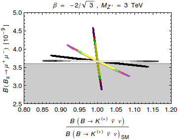
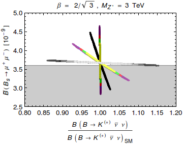
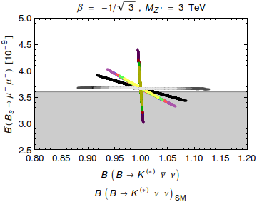
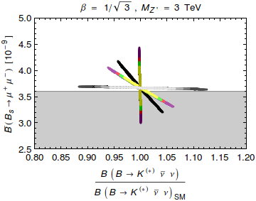
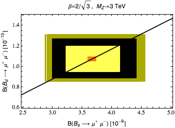
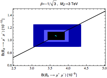
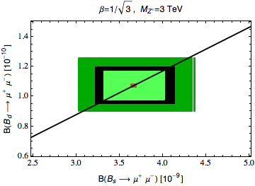
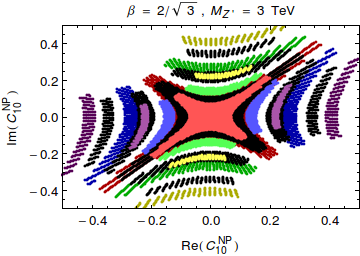
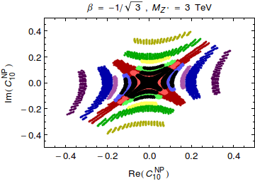
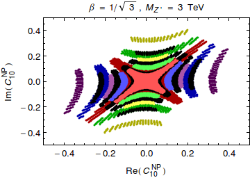
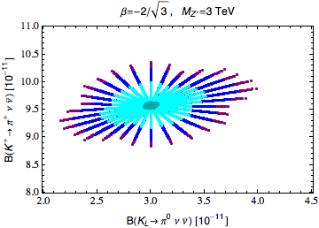
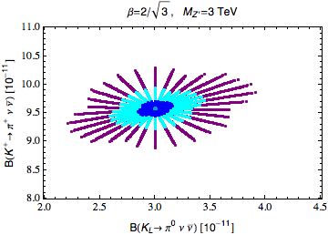
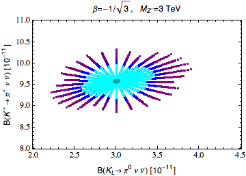
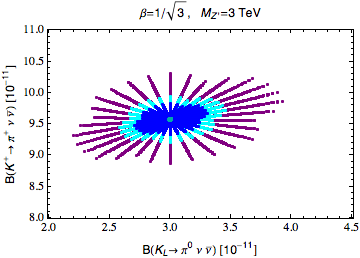
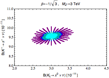
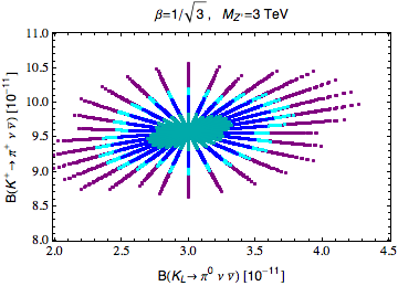
There is no specific correlations between the branching ratios for and decays and this implies significant departures from CMFV relation between their branching ratios. We show as an example in Fig. 6 the results for values of and fermion representations . The case without mixing, that is pure contributions, represented by the black regions allows to see that the presence of boson contributions in both decays represented by departure from these areas can be significant as could be deduced from previous results.
-
•
As seen in Fig. 7 boson contributions have significant effect on the size of CP violation in that originates from a non-vanishing imaginary part of , in constrast to that is real. As the tests of CP-violating effects in this decay are in the distant future we only show the results for in this case.
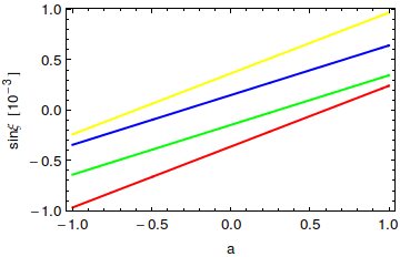
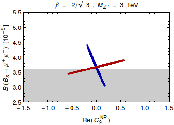
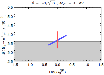
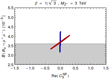
Finally, we look at the decay and its correlation with . The interest in the analysis of this decay lies in the fact that in contrast to and that in 331 models are sensitive only to and , respectively, the branching ratio for depends on both coefficients. Moreover, lattice calculations of the relevant form factors are making significant progress here [35, 36] and the importance of this decay will increase in the future.
Neglecting the interference between NP contributions the formula for the differential branching ratio confined to large region ()444This formula is based on [33] and a recent update. Straub, private communication. reduces in 331 models in units of to
| (48) |
The relevant Wilson coefficients are given in (44) and (45). This formula describes triple correlation between , and which constitutes an important test for the models in question. In the absence of mixing this triple correlation involving the rate for at large can be found in Fig. 13 in [4] for the case of representations.
The error on the first SM term is estimated to be [35, 36]. This should be compared with the LHCb result [37]
| (49) |
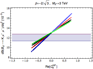
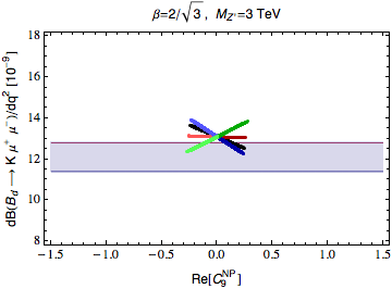
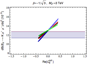
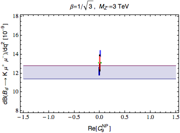
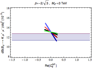
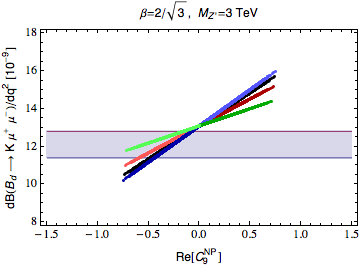
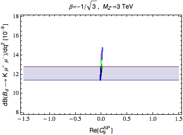
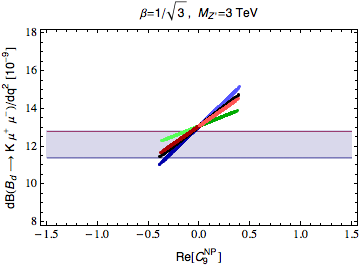
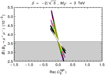
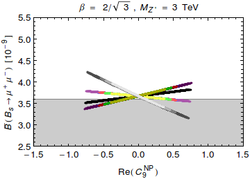
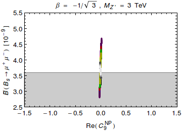
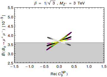
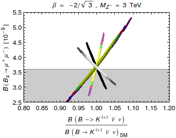
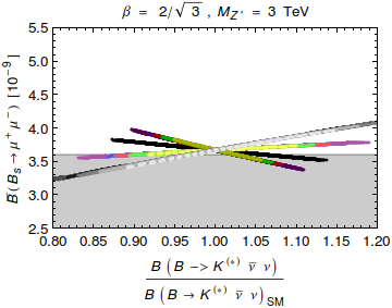
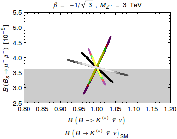
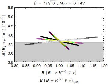
In Fig. 8 we generalize this result to include mixing and in Fig. 9 we present corresponding results for . As in the case of Figs. 2 and 3 we obtain straight lines with slopes depending on the values of and . The case of no mixing is again shown by black lines. In these plots the colour coding is:
| (50) |
with lighter colours showing when is enhanced and with darker ones when it is suppressed with respect to the SM prediction.
There are two striking differences between these results an those in Figs. 2– 5. The effects of mixing in Figs. 8 and 9 are significantly smaller and consequently the symmetry in (35) is less broken.
At this point we would like to emphasize that all the results described until now do not take into account the constraints from electroweak precision tests. In Section 5 we will analyze which lines in Figs. 2– 5, 8 and 9 survive the latter tests and which not. In any case with , as demonstrated in [4], the bounds from LEP-II and LHC are satisied.
3.3 Numerical Results for Rare Decays
In our recent paper [38] we have reemphasized the strong dependence of rare decay branching ratios on the values of the elements of the CKM matrix and . This dependence is particularly strong in the case of as seen in Table 3 of that paper. While in [38] we have studied six scenarios for and in 331 models most of these scenarios are ruled out by . In fact as already pointed out in [3] NP effects in are rather small when constraints from mixing are taken into account. Therefore the 331 models can only be made consistent with data on for values of and for which the SM prediction for is rather close to this data. Then only scenarios and in [38]
| (51) | ||||
| (52) |
survive the constraint in 331 models as then for central values of remaining parameters and , respectively. This is close to the experimental value so that there is no problem in fitting the data.

Now in [4] and in the analysis of decays in the present paper we have used the values
| (53) |
which implies that is rather close to the choice above and as it also allows to satisfy the constraint, we will use these values for rare decays and .
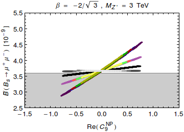
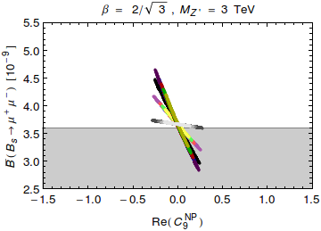
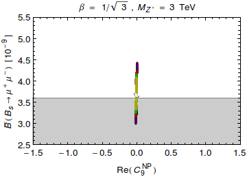
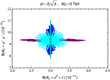
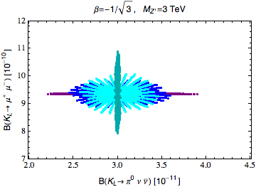
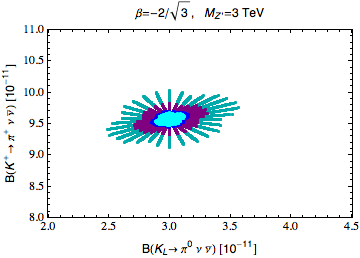
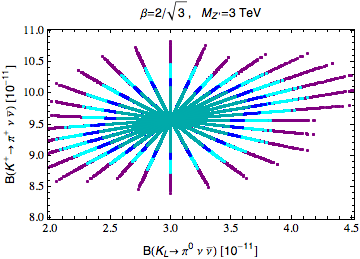
In Figs. 10 and 11 we show various correlations between rare decay branching ratios for the four 331 models considered for the case, three values of and the case without mixing which represents sole contributions. While these plots are self-explanatory, in particular when considered simultaneously with Table 1, we would like to emphasize a number of most important features in them. These are:
-
•
A rather striking feature is the cancellation of and contributions to the branching ratios for and for so that in this case one obtains basically the SM prediction independently of the value of . On the contrary in the case of for and in particular for negative NP effects are enhanced through mixing. This difference between decays with neutrino and muons in the final state has been also seen in the case of decays.
-
•
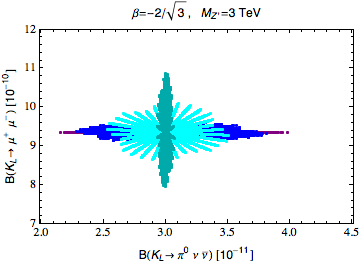
A different behaviour is observed for . In the case of and for models with and there is a destructive interference between and contributions decreasing somewhat NP effects due to exchange alone. For and , on the other hand, the corresponding interference is constructive and NP effects are increased. On the contrary the effects of mixing for in are rather small.
-
•
For NP effects in and increase but they basically disappear in the case .
-
•
On the whole NP effects except for the case of and are rather small and it will be difficult to distinguish them from SM expectations unless parametric uncertainties decrease by much and experimental data will be very precise.
Considering the case of representations one can deduce from Table 2 that the symmetry in (35) is significantly broken in rare decays but the size of NP effects is similar to the case. As an example we show in Fig. 12 the correlation between the branching ratios for and for . In particular for and NP effects are significant.
But the main message from our analysis of rare and decays is that neglecting contributions in decays governed by axial vector couplings to muons or left-handed couplings to neutrinos is not justified and observing significant NP effects in would imply and only small effects in and . On the other hand confirming SM predictions for to high degree would in 331 models for still allow for modest by significant departures from SM expectations for these decays and imply for 331 models .
Again the results just described do not take into account the constraints from electroweak precision tests and it will be interesting to see in Section 5 the impact of the latter tests on them.
4 The Ratio
4.1 Preliminaries
Recently we have presented a new analysis of within the SM and models with tree-level and boson exchanges [38]. Several of the formulae presented in that paper can be directly used in the context of the 331 models and consequently our presentation will be rather brief. In 331 models we have
| (54) |
where the formula for the SM contribution, an update of the original one in [39], is given in (53) of [38].
4.2 Contribution
This case is simple as the only thing to be done is to introduce shifts in the functions , and that enter the SM model contribution to . Using the results of Section 7 in [38] together with the relation (3) we find
| (55) |
where and . Replacing then the functions , and by
| (56) |
in the formula (53) for in [38] allows to take automatically the first two contributions in (54) in 331 models into account.
4.3 Contribution
Using the general formulae for the flavour diagonal couplings to quarks in [3, 4] we find that in LO as far as penguin operators are concerned the only non-vanishing Wilson coefficients at are the ones of the known QCD penguin operator , the known electroweak penguin operator as well as of the operator
| (57) |
which is present due to different couplings of to the third generation of quarks. Their coefficients are given in 331 models as follows
| (58) |
| (59) |
| (60) |
with defined in (11). We recall that these results are valid for fermion representation . For one just has to reverse the sign in front of according to the rules outlined in Section 2.2.
The coefficients of these three operators at are of the same order. Yet, when QCD renormalization group effects are included and the size of hadronic matrix elements relevant for are taken into account we find that the and contributions can be neglected leaving the left-right electroweak penguin operators
| (61) |
as the only relevant operators in contribution to in 331 models. However, even if at LO the Wilson coefficient of vanishes at , at used in our numerical analysis of its Wilson coefficient is of the same order as . Indeed the relevant one-loop anomalous dimension matrix in the basis is given by
| (62) |
Performing the renormalization group evolution from to we find using explicit formulae in [38]
| (63) |
Due to the large element in the matrix (62) and the large anomalous dimension of the operator represented by the element in (62), the two coefficients are comparable in size. But the matrix element is colour suppressed which is not the case of and within a good approximation we can neglect the contributions of . In summary, it is sufficient to keep only contributions in in 331 models.
The relevant isospin amplitude in decays necessary to calculate contribution to is given as follows
| (64) |
where [38]
| (65) |
with from lattice QCD [40].
In our numerical analysis we will use for the quark masses the values from FLAG 2013 [41]
| (66) |
Then at the nominal value we have
| (67) |
The final expression for contributions is given by
| (68) |
where [42]
| (69) |
In evaluating (68) we use, as in the case of the SM, the experimental values for and :
| (70) |
As NP contributions to , both due to and , are dominated by the operator , the ratio of these contributions depends with high accuracy simply on the ratio of in these two contributions. This allows then to derive a simple relation
| (71) |
where ()
| (72) |
This expression is valid for fermion representation . For for a given one should just remove the overall minus sign in this expression as the in front of the parenthesis enters the coupling. The expression in the parenthesis comes from mixing and is independent of the fermion representation. The factor summarizes the difference in renormalization group effects for and contributions. QCD renormalization of gives alone and additional small suppression comes from the running of electroweak parameters. We list the values of in the last row of Tables 1-3. Evidently dominates NP contributions to implying that mixing effects are small in this ratio. The two exceptions are the case of and and the case of and for which contribution reaches of the one.
4.4 Numerical Analysis of
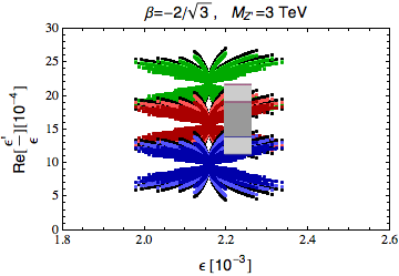

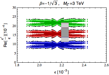
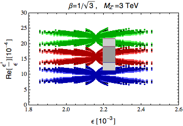


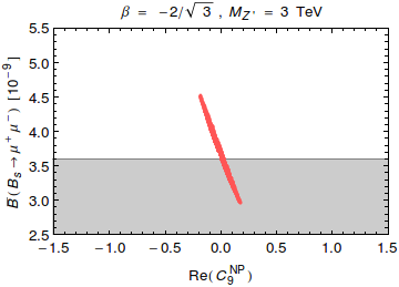
In Fig. 13 we show versus . We make the following observations:
-
•
331 models for all values of are consistent with the data for provided represented by red colour.
- •
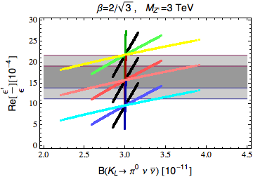
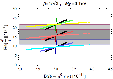
In Fig. 14 we show versus for fermion representations . We observe that the correlation between these two observables is very strict as is linear in the imaginary parts of the flavour violating and couplings and NP contribution to is dominated by the interference of the SM and NP amplitude. Consequently is also linear in these couplings. Two interesting features of these plots should be emphasized
-
•
while for negative the ratio decreases with increasing , for positive it increases with increasing . The latter property is rather rarly found in other extensions of the SM.
-
•
The effects of mixing are clearly visible, in particular for . They originate dominantly in the ones present in .
-
•
As already known from Fig. 13 the agreement of the theory and the data is best for .
5 Electroweak Precision Observables
5.1 Preliminaries
The modifications of the boson couplings due to mixing in 331 models can be tested through electroweak precision measurements at LEP-I and SLD and such an analysis can be found in [9] and recently in [43]. As our formula for differs from the one used in these papers we want to analyze the impact of mixing on most important electroweak precision observables (EWPO) and study their dependence on , and the choice of fermion representations. Thus our next goal is to construct three tables for the shifts of a number of EWPO relative to SM predictions. This will eventually allow us to investigate the correlations between NP effects in EWPO and flavour observables. In these tables we will set . As the shifts in question are inversely proportional to it is straight forward to find out what happens for other values of .
Transparent analyses of the effects of mixing in EWPO can be found in [44, 29, 45]. We will follow here the general analysis in [29] and to this end it is useful to note that our couplings of a given fermion to and differ from the couplings and used in that paper by an overall factor:
| (73) |
| (74) |
For couplings we then have
| (75) |
where is the third component of the weak isospin of the fermion and its electric charge. Our effective couplings in (7) are then related to the analogously defined ones in [29] simply as follows
| (76) |
Due to the mixing the parameter, defined by
| (77) |
receives tree-level contribution which for is given by [44, 29, 45]
| (78) |
This shift is strictly positive and . Consequently it is of the same order as the mixing effects in the effective couplings in (7) so that it has to be taken into account. On the other hand we conclude on the basis of [46] that in 331 models studied by us the oblique contributions involving new heavy charged gauge bosons, scalars and fermions can be neglected when their masses are in the few TeV regime. Consequently the shift in due to NP in these models is dominated by given above.
Keeping fixed as input parameters , and , the effective Weinberg angle in (77) is modified due to the shift in as follows [44, 29]
| (79) |
It should be noted that this shift is strictly negative and this property is valid for any model. Yet, as we will see below, this does not mean that the shift in the so-called effective is negative in any model as the contributions to couplings that are proportional to are clearly model dependent. Some aspects of this dependence has been already analyzed in the context of 331 models in [43]. Our improved formula for in (10) and the gained insight on the correlations between mixing and FCNCs processes allows us to have another look at this issue thereby also generalizing the analysis in [43].
Next denoting a given observable by the shift due to mixing can be linearized in and as follows [29, 45]
| (80) |
Here the coefficients are universal and depend only on the SM parameters and couplings. On the other hand depend on the diagonal -couplings in (7). Direct contributions to EWPO are negligible.
We will list the general formulae for the coefficients and below but rather then giving numerical values for them as done in [29] we will calculate the shifts in EWPO for different values of , and the fermion representations and for . To this end we will proceed as follows
-
•
We will calculate a number of EWPO as functions of the effective diagonal -couplings in (7) in 331 models using tree-level formulae. In doing this one should remember that in addition to the direct contribution of to the effective couplings leading to the second term in (80) also the shift in entering the vector coupling has to be taken into account. That is in the coupling to a fermion one should make additional replacement:
(81) with given in (79). This contribution to the shift is represented by the first term (80).
-
•
Denoting the result for a given observable calculated in this manner by we can simply calculate the shift due to NP by subtracting the pure SM contributions at tree level:
(82) As the mixing effects are very small the higher order terms generated by this numerical procedure are tiny and consequently one would obtain quite generally very similar results by using the linearized form in (80) as done in [29, 45]. Moreover as stressed in [29] in certain models such a linearized expression could not be sufficiently precise and using (82) from the start takes such effects into account.
-
•
For the SM contributions we will use the most recent values for EWPO that include electroweak radiative corrections. Even if the interference terms between SM and NP contributions will not include these corrections, this procedure is justified in view of the smallness of NP effects in 331 models considered by us.
-
•
Comparing SM results with the data we will be able to identify the pattern of deviations from SM predictions and see for which values of , and fermion representations the 331 models can improve the agreement of the theory with the data and what does this imply for our analysis of flavour violating effects.
5.2 Basic Formulae for EWPO
The tree level formula for the partial widths is given by
| (83) |
with for quarks and for leptons. The additional overall factor relative to formula (2.8) in [29] takes into account the difference in the definitions of the vector and axial-vector couplings summarized above. Defining next we have
| (84) |
While we do not distinguish between for quark contributions and contributions from lighter quarks as such effects are taken into account in the full SM contribution, we separate NP quark contribution to from the one of and as transformation properties of the third generation of quarks under are different compared to the the first two generations. See the Lagrangian (63) in [3]. This difference has to be taken into account in all observables involving the quark.
Of interest are then the ratios and the peak cross sections defined as follows
| (85) |
Note that the definition of differs from the one of and . For the asymmetries we have
| (86) |
and for the forward-backward asymmetry
| (87) |
We would like to warn the reader that similar to [29] our vector and axial-vector couplings for and are defined in terms of left-handed and right-handed ones as follows:
| (88) |
Consequently the axial-vector couplings differ by sign from the ones used in PDG. This implies that also asymmetries differ by sign from PDG and in Table 7 when quoting PDG values we adjusted their definition to our.
From these formulae it is straightforward to derive general analytical formulae for the coefficients and in (80), valid in any model. We first find in the case of the partial width
| (89) |
where the second term in is the universal correction from the shift in in the overall factor in (83).
In the case of the asymmetry the corresponding expressions read
| (90) |
Our results in (89) and (90 agree with the ones one would derive from formulae (6.5)-(6.6) and (7.4)-(7.7) in [44] by dividing them by and , respectively.
For and we find respectively
| (91) |
and
| (92) |
In these formulae and are just tree-level SM contributions.
We observe that indeed the coefficients depend only on SM couplings and the first term in (80) feels the presence of only through , while the second one has additional dependence on the diagonal couplings. While these formulae allow an easy comparison with the analyses in [44, 29, 45], in numerical calculations it is easier to use directly (82).
5.3 Numerical Results
| 1.149(4.408) | 0.226(1.714) | 0.0713( 0.255) | 0.670(-0.0455) | |
| (LEP) | ||||
| 0.0919(1.715) | 0.0554( 1.018) | |||
| (LEP) | 13.04(27.57) | 13.26(18.14) | 13.77(15.41) | 14.74(15.06) |
| (LEP) | 13.59(15.72) | 14.78(16.20) | 23.03(19.37) | 48.97(28.94) |
|---|---|---|---|---|
| Quantity | Input Data | SMfit | Pull |
|---|---|---|---|
| [nbarn] | |||
In Tables 4-6 we list the shifts in a number of observables as functions of , for the fermion representations and . In Table 7 we summarize SM predictions for these observables, the corresponding data and the pulls as presented after Higgs discovery in [47].
In what follows it will be useful to denote by MI, with a given I=1,..24, a particular 331 model in which , and fermion representations are fixed. The index I numbers the column in Tables 4-6 corresponding to a given model in order of its appearance. Thus we deal with 24 models that we specify in Table 8 to make their identification easier. For instance M5 denotes the model with , and .
| MI | scen. | MI | scen. | MI | scen. | ||||||
|---|---|---|---|---|---|---|---|---|---|---|---|
| M1 | 1 | M9 | 1 | M17 | 0.2 | ||||||
| M2 | 5 | M10 | 5 | M18 | 0.2 | ||||||
| M3 | 1 | M11 | 1 | M19 | 0.2 | ||||||
| M4 | 5 | M12 | 5 | M20 | 0.2 | ||||||
| M5 | 1 | M13 | 1 | M21 | 0.2 | ||||||
| M6 | 5 | M14 | 5 | M22 | 0.2 | ||||||
| M7 | 1 | M15 | 1 | M23 | 0.2 | ||||||
| M8 | 5 | M16 | 5 | M24 | 0.2 |
In order to judge the quality of a given model and compare it with the performance of the SM we define for each observable the pulls and as follows
| (93) |
The pulls are the usual ones and their values are given in the last column in Table 7. In principle in order to calculate such pulls for every 331 model MI considered by us we would have to repeat the fit of [47] for all models including also other observables that are sensitive to new charged gauge bosons. Such an analysis is clearly beyond the scope of our paper. As are fixed in a given MI, that is do not introduce new parameters, we expect that such a simplified procedure should give us a correct, even if rough, picture of what is going on.
In order to identify favourite 331 models, as far as electroweak observables are concerned, we define the measures
| (94) |
The first SM value is based on Table 7 using the average of LEP and SLD values for while the one in the parentheses is obtained by using as curiosity only the LEP value. The values of for 331 models are given in Tables 4-6. The models with smallest are favoured, while the ones with with largest disfavoured.
Inspecting these results we make first the following observations when the average of LEP and SLD values for is used.
-
•
All models give small contributions to and and consequently agree with the data.
-
•
All models give rather small contributions to and consequently cannot remove the small pull present in the SM. Moreover, M21 and M23 soften the agreement of the theory with data.
-
•
The sizable discrepancy of the SM with the data on cannot be removed in any model. It can be softened by in M2 and M10 and visibly increased in models M21-M24.
We concentrate then our discussion on the remaining observables, where NP effects turn out to be larger. We find
-
•
In most models NP effects in are small in agreement with data. Deviations larger than are only found in M2, M10 and M23.
-
•
In the case of the agreement with data is significantly improved in the case of M1, M2, M4, M9, M10, M12 but worsened visibly in M7, M15 and all models with , that is M17-M24.
-
•
Interestingly in the case of all the models with improve the agreement of the theory with data and this also applies to M7 and M15, while the remaining models slightly worsen the agreement.
-
•
On the contrary in the case of and the models with and are performing much better than the ones with . Moreover they perform better than the SM. However, this depends, as discussed below, whether one takes into account the SLD value for or not.
-
•
Concerning and the favourite models listed below introduce only a very small shift to the SM values not improving the status of the theory, while several models, in particular M2, M4, M7, M10, M12, M21 and M23 worsen the agreement with the data. This is also the case of two favoured models below, M14 and M16 but they compensate it through better results for than obtained within the SM.
The final verdict is given by the values of in Tables 4-6. We observe that seven 331 models have . These are in the order of increasing
| (95) |
with the first five performing better than the SM while the last two having basically the same . The models with odd index I correspond to and the ones with even one to . We list the pulls in these seven models in Table 9.
| Pull |
|
|
|
|
|
|
|
|||||||||||||||||||||
|---|---|---|---|---|---|---|---|---|---|---|---|---|---|---|---|---|---|---|---|---|---|---|---|---|---|---|---|---|
| 0.099 | 0.338 | 0.271 | 0.546 | 0.164 | 0.204 | 0.055 | ||||||||||||||||||||||
| 1.216 | 1.187 | 1.490 | 1.352 | 1.389 | 0.831 | 0.920 | ||||||||||||||||||||||
| 0.067 | 0.067 | 0.075 | 0.071 | 0.072 | 0.056 | 0.059 | ||||||||||||||||||||||
| 0.979 | 0.987 | 0.901 | 0.941 | 0.930 | 1.088 | 1.063 | ||||||||||||||||||||||
| 2.682 | 2.706 | 2.463 | 2.574 | 2.545 | 2.991 | 2.919 | ||||||||||||||||||||||
| 0.053 | 0.063 | 0.058 | 0.071 | 0.052 | 0.064 | 0.060 | ||||||||||||||||||||||
As seen in this table all favoured models improve the agreement of the theory with data on . This is in particular the case of M9 and this fact is primarily responsible why M9 wins the competition as it does reasonably well for other observables. We also observe that all favoured models, except M8, improve the agreement of theory with data on and . However the models M14 and M16 which perform best in this respect are not the top models as they perform worse than the first ones on other observables which basically do not provide any improvements on these asymmetries. The reason is that M14 and M16 experience difficulties with and , as stated above, making the agreement of the theory with data to be worse than in the SM.
Yet, as discussed below, our analysis confirms the general findings of Richard [43] that in 331 models the departure of the data on and from their SM values is correlated within 331 models with the anomaly, even if the model M2 which he studied is basically excluded by other electroweak data when correct expression for is used. This is in particular the case of and . Otherwise this model is interesting as it removes the discrepancy of the SM with the data on .
An important result of our analysis is the weak performance of models with , although the models M17-M20 cannot be excluded. The models which definitely have difficulties with electroweak precision data are
| (96) |
Looking at these results we conclude that from the point of view of electroweak precision tests the following combinations of the values of , and fermion representations are favoured.
-
•
Three models with and for . For this is M3 with and for M9 and M11 for and , respectively.
-
•
Four models with and for . For these are M6 and M8 for and , respectively and analogously M14 and M16 in the case for .
It should be emphasized that all these seven models pass the present electroweak tests for as well as the SM or in five cases even better than it. Even if the models with perform slightly better than the ones with it is not possible on the basis of alone to identify the winner among them. On the other hand one day this should be possible on the basis of the Table 9 once various questions related to measurements at LEP and SLD will be clarified. As demonstrated below flavour physics can offer definite help in this context.
In the latter context it is interesting to observe that if the LEP result for would be the true one five models on the list of favourites in (95) would remain
| (97) |
with the first three performing better than the SM. M14 and M16 are not present anymore on this list because they favoured SLD result. Instead M13 and in particular M17 with are among favourites. As we will discuss below M17 has a unique property among the favourites as far as flavour physics is concerned.
5.4 The issue of
In testing the SM one can define by using SM tree-level expression for . This parameter is most precisely extracted from the data on and but also from . Unfortunately the determinations of from these observables are really not in agreement with each other. On one hand in the case of we have [48, 43]
| (98) |
and from forward-backward asymmetries and one finds respectively
| (99) |
This implies roughly discrepancy between the two most precise determinations. The resulting values from all data as given in Table 7 are
| (100) |
Consequently there is some preference for the positive shift in relative to the best SM value.
Until now we did not look at in 331 models and calculated , , and other observables directly to judge the quality of a given model on the basis of them. But it is instructive to calculate the shift of due to NP contributions for 24 models considered by us using the operative definition [48]
| (101) |
where in the effective vector couplings the shift (81) has to be included. An extensive discussion of can be found in [48] where further references can be found. See also [43]. In writing (101) we have adjusted the sign in the formula (8.3) in [48] to our definition of the axial-vector coupling.
The shift in in 331 models comes first from the shift of which as seen in (79) is negative in 331 models and in any model. But in addition to this shift, which comes from and affects only vector couplings, both vector and axial-vector couplings receive modifications from the mixing with , that is the shifts in the couplings proportional to and involving couplings.
The result of this exercise is given in the last rows in Tables 4-6. The striking feature is that out of 24 models 19 give a negative shift of , while only 7 a positive one. These are M8, M13, M15, M17 and M19.
It is not surprising that M8, M13 and M17 perform here so well as they are on the list of LEP favourites in (97). What is remarkable that M8 is the only among our favourite models in (95) that gives a positive shift of . But this shift being is totally negligible. Yet, this model similar to all models with positive shift is fully compatible with the experimental value in (100).
We also note that models M14 and M16 on our list of favourites give
| (102) |
where we have added the corresponding shifts to the SM value in (100). These values are within from the central value of from the SLD.
We also confirm qualitatively the finding in [43] that the model M2 provides a shift that results in close to the SLD result. We find and for and , respectively. For the SLD result can be well reproduced. However, this model has problems with other observables as we have seen above.
While we do not think that just looking at offers a fully transparent test of a given extension of the SM, the rather different values of this parameter extracted from different observables calls for future improved measurements of EWPO which hopefully one day will be possible at a future ILC. This, as stressed in [43], could offer powerful tests of 331 models.
5.5 Implications for Flavour Physics
Our analysis of EWPO identified a group of seven models among 24 considered by us and the question arises whether flavour physics could distinguish between them. As we will now discuss our analysis in previous sections demonstrates this rather clearly and having the plots presented there we can summarize how the seven models in question could be distinguished by flavour observables in the coming flavour precision era.
Let us first summarize the main message from our analysis of EWPO which is related to the fact that the values are disfavoured:
-
•
Significant NP effects in and decays to neutrinos seem rather unlikely, even if the branching ratio for could still be modified by . In turn due to the correlation with also NP effects in this ratio are predicted to be small implying that in order to agree with data. On the other hand as discussed in our recent paper [38] the required precise value of this parameter depends on the values of and .
-
•
The most interesting NP effects are found in and and we will confine the discussion of the favourite models in (95) to these decays.
The selection of favourite models and the comments just made imply that it is sufficient to look at Figs. 2 and 3 for and , respectively. The results for the seven favourite models can be found there with only the results in the upper left panel in Fig. 2 being disfavoured. In the remaining seven panels in these two figures, the results for our favourite models are simply identified by selecting the line (lighter colours) in the case of and the line (darker colours) in the case of . The main implications for rare decays are then as follows:
-
•
A significant suppression of and significant negative shift in cannot take place simultaneously. This would be possible in M2 but this model belongs to disfavoured ones by our EWPO analysis.
-
•
For softening the anomaly the most interesting is the model M16, that is the model with , and . See upper right panel in Fig. 3. The usual statements present in the literature [26, 4, 43] that the 331 models with negative are most powerful in this case apply to representations. But as our analysis shows the model M2 with considered by us in [4] is disfavoured by the EWPO analysis.
- •
-
•
The remaining four models, in fact the four top models on our list of favourites in (95), do not provide any explanation of anomaly but are interesting for decays. These are M6, M8, M9 and M11, the first two with and the last two with fermion representation. The differences between these models as far as is concerned are most transparently seen in Figs. 4 and 5 from which we conclude that the strongest suppression of the rate for can be achieved in M8 and M9. M8 result is shown in the right upper panels in Figs. 2 and 4 and M9 result in the left upper panels of in Figs. 3 and 5. In fact these two models are the two leaders on the list of favourites in (95). The suppression of the rate is smaller in M6 and M11 as seen in lower right and lower left panels in Figs. 2 and 3, respectively.
We observe that flavour physics can clearly distinguish between the favourite models selected by EWPO analysis. We summarize it in Fig. 15, where only the results in the seven favourite models are shown. If the anomaly will persist the winner will be M16 which is represented in this figure by the dark red line in the upper right panel. If it disappears but suppression of the rate for will be required the winners will be M8 and M9, the blue and red lines in the upper right and upper left panel in Fig. 15, respectively. It is interesting that the combination of future flavour data and EWPO tests can rather clearly indentify one or two favourite 331 models among 24 cases considered by us.
An interesting situation would also arise if the LEP result for would turn out to be the correct one. In this case M14 and M16 are no longer among favourites as seen in (97) and are replaced by M13 and M17. M13 is a good replacement for M14 as it also allows moderate softening of the anomaly as seen in the right lower panel in Fig. 3. But more interesting is M17. Indeed as seen in the upper left panel in Fig. 2 for (gray line) the anomaly can be softened as much as it was possible in the case of M16. But as seen in the upper left panel in Fig. 10 (purple line) in this model with representations also significant NP effects in are possible. Smaller NP effects, as seen in Fig. 12, are found in the case of but is not among the favourite models anyway. All this again shows an important interplay between flavour observables and electroweak precision tests.
6 Summary and Conclusions
In this paper we have addressed the question whether in 331 models the FCNCs due to tree-level exchanges generated through mixing could play any significant role in flavour physics. Actually it is known from the flavour analyses of Randall-Sundrum models with custodial protection (RSc) [49, 50], that while processes are governed by heavy Kaluza-Klein gauge bosons with and without colour, NP contributions in processes are governed by induced right-handed flavour-violating couplings.
Here we analyzed several 331 models which have a much smaller number of parameters than RSc and this allows to see more transparently various NP effects than in the latter scenario. As our basic formula for the in 331 model differs from the one found in the literature [8, 14, 43] we have reconsidered some aspects of constraints from EWPO. Moreover we have identified for the first time various correlations between flavour and electroweak physics that depend on the parameters of 331 model, in particular, , , and the fermion representations.
As far as flavour physics is concerned our main findings are as follows:
-
•
NP contributions to transitions and decays like are governed by tree-level exchanges. Therefore for these processes our analysis in [4] remains unchanged. But as we summarize below our analysis of EWPO casts some shadow on some of these models.
-
•
On the other hand for decays contributions can be important. We find that for these contributions interfere constructively with contributions enhancing NP effects, while for low contributions practically cancel the ones from . Similar dependence on is found for .
-
•
Similarly boson tree-level contributions to and decays with neutrinos in the final state can be relevant but in this case the dependence is opposite to the one found for . We find that for these contributions practically cancel the ones from but for low contributions interfere constructively with contributions enhancing NP effects. In particular as seen in Figs. 10 and 11 in the case of NP effects can amount to at the level of the branching ratio when the constraints from EWPO are not taken into account.
- •
-
•
Our analysis of is to our knowledge the first one in 331 models. Including both and contributions we find that the former dominate. But NP effects are not large and in order to fit the data is favoured.
-
•
We also find a strict correlation between and . The interesting feature here, as seen in Fig. 14, is the decrease of with increasing for negative and its increase with increasing for positive .
- •
As far as electroweak physics is concerned our main findings are as follows:
-
•
Seven among 24 combinations of , and fermion representation or provide better or equally good description of the electroweak precision data compared with the SM. However, none of these models allows for the explanation of the departures of and from the SM but several of them improve significantly the agreement of the theory with the average of SLD and LEP data for .
-
•
Among these models none of them allows to simultaneously suppress the rate for and soften the anomaly.
-
•
On the other there are few models which either suppress the rate for or soften the anomaly.
-
•
None of these models allows significant NP effects in and decays with neutrinos in the final state although departures by relative to the SM prediction for the rate of are still possible.
-
•
Assuming that the LEP result for is the correct one, we have found that in this case NP effects in are larger than when both LEP and SLD results are taken into account.
Our analysis shows that the interplay of flavour physics and EWPO tests can significantly constrain NP models, in particular those with not too many free parameters. We are looking forward to coming years in order to see whether the 331 models will survive improved flavour data and in particular whether will be discovered at the LHC. The correlations presented by us should allow to monitor transparently future developments in the data.
Acknowledgements
We would like to thank Christoph Niehoff and David Straub for asking us about the size of tree-level contributions to FCNC processes in 331 models. We also thank Guido Altarelli, Jernej Kamenik, Ulrich Nierste, Francois Richard, R. Martinez and F. Ochoa for interesting discussions. This research was done and financed in the context of the ERC Advanced Grant project “FLAVOUR”(267104) and was partially supported by the DFG cluster of excellence “Origin and Structure of the Universe”.
References
- [1] F. Pisano and V. Pleitez, An SU(3) x U(1) model for electroweak interactions, Phys.Rev. D46 (1992) 410–417, [hep-ph/9206242].
- [2] P. H. Frampton, Chiral dilepton model and the flavor question, Phys. Rev. Lett. 69 (1992) 2889–2891.
- [3] A. J. Buras, F. De Fazio, J. Girrbach, and M. V. Carlucci, The Anatomy of Quark Flavour Observables in 331 Models in the Flavour Precision Era, JHEP 1302 (2013) 023, [arXiv:1211.1237].
- [4] A. J. Buras, F. De Fazio, and J. Girrbach, 331 models facing new data, JHEP 1402 (2014) 112, [arXiv:1311.6729].
- [5] D. Ng, The Electroweak theory of SU(3) x U(1), Phys.Rev. D49 (1994) 4805–4811, [hep-ph/9212284].
- [6] R. A. Diaz, R. Martinez, and F. Ochoa, The Scalar sector of the SU(3)(c) x SU(3)(L) x U(1)(X) model, Phys.Rev. D69 (2004) 095009, [hep-ph/0309280].
- [7] J. T. Liu and D. Ng, Lepton flavor changing processes and CP violation in the 331 model, Phys.Rev. D50 (1994) 548–557, [hep-ph/9401228].
- [8] R. A. Diaz, R. Martinez, and F. Ochoa, SU(3)(c) x SU(3)(L) x U(1)(X) models for beta arbitrary and families with mirror fermions, Phys.Rev. D72 (2005) 035018, [hep-ph/0411263].
- [9] F. Ochoa and R. Martinez, mixing in models with beta arbitrary, hep-ph/0508082.
- [10] J. T. Liu, Generation nonuniversality and flavor changing neutral currents in the 331 model, Phys.Rev. D50 (1994) 542–547, [hep-ph/9312312].
- [11] J. A. Rodriguez and M. Sher, FCNC and rare B decays in 3-3-1 models, Phys.Rev. D70 (2004) 117702, [hep-ph/0407248].
- [12] C. Promberger, S. Schatt, and F. Schwab, Flavor Changing Neutral Current Effects and CP Violation in the Minimal 3-3-1 Model, Phys.Rev. D75 (2007) 115007, [hep-ph/0702169].
- [13] J. Agrawal, P. H. Frampton, and J. T. Liu, The Decay in the 3-3-1 model, Int.J.Mod.Phys. A11 (1996) 2263–2280, [hep-ph/9502353].
- [14] A. Carcamo Hernandez, R. Martinez, and F. Ochoa, Z and Z’ decays with and without FCNC in 331 models, Phys.Rev. D73 (2006) 035007, [hep-ph/0510421].
- [15] C. Promberger, S. Schatt, F. Schwab, and S. Uhlig, Bounding the Minimal 331 Model through the Decay , Phys.Rev. D77 (2008) 115022, [arXiv:0802.0949].
- [16] M. Singer, J. Valle, and J. Schechter, Canonical Neutral Current Predictions From the Weak Electromagnetic Gauge Group SU(3) X (1), Phys.Rev. D22 (1980) 738.
- [17] J. Valle and M. Singer, Lepton Number Violation With Quasi Dirac Neutrinos, Phys.Rev. D28 (1983) 540.
- [18] S. M. Boucenna, S. Morisi, and J. W. F. Valle, Radiative neutrino mass in 331 scheme, arXiv:1405.2332.
- [19] A. J. Buras, F. De Fazio, and J. Girrbach, The Anatomy of Z’ and Z with Flavour Changing Neutral Currents in the Flavour Precision Era, JHEP 1302 (2013) 116, [arXiv:1211.1896].
- [20] A. J. Buras and J. Girrbach, Left-handed Z’ and Z FCNC quark couplings facing new data, JHEP 1312 (2013) 009, [arXiv:1309.2466].
- [21] LHCb Collaboration Collaboration, R. Aaij et. al., Differential branching fraction and angular analysis of the decay , JHEP 1308 (2013) 131, [arXiv:1304.6325].
- [22] LHCb collaboration Collaboration, R. Aaij et. al., Measurement of form-factor independent observables in the decay , Phys.Rev.Lett. 111 (2013) 191801, [arXiv:1308.1707].
- [23] LHCb collaboration Collaboration, R. Aaij et. al., Measurement of the branching fraction and search for decays at the LHCb experiment, Phys.Rev.Lett. 111 (2013) 101805, [arXiv:1307.5024].
- [24] CMS Collaboration Collaboration, S. Chatrchyan et. al., Measurement of the branching fraction and search for with the CMS Experiment, Phys.Rev.Lett. 111 (2013) 101804, [arXiv:1307.5025].
- [25] Combination of results on the rare decays from the cms and lhcb experiments, Tech. Rep. CMS-PAS-BPH-13-007, CERN, Geneva, 2013.
- [26] R. Gauld, F. Goertz, and U. Haisch, An explicit Z’-boson explanation of the anomaly, JHEP 1401 (2014) 069, [arXiv:1310.1082].
- [27] P. Langacker, The Physics of Heavy Gauge Bosons, Rev.Mod.Phys. 81 (2009) 1199–1228, [arXiv:0801.1345].
- [28] J. Erler, P. Langacker, S. Munir, and E. Rojas, Improved Constraints on Z-prime Bosons from Electroweak Precision Data, JHEP 0908 (2009) 017, [arXiv:0906.2435].
- [29] G. Altarelli, N. Di Bartolomeo, F. Feruglio, R. Gatto, and M. L. Mangano, R(b), R(c) and jet distributions at the Tevatron in a model with an extra vector boson, Phys.Lett. B375 (1996) 292–300, [hep-ph/9601324].
- [30] R. Martinez and F. Ochoa, Constraints on 3-3-1 models with electroweak Z pole observables and Z’ search at LHC, arXiv:1405.4566.
- [31] C. Bobeth, M. Gorbahn, T. Hermann, M. Misiak, E. Stamou, et. al., in the Standard Model, arXiv:1311.0903.
- [32] S. Descotes-Genon, J. Matias, and J. Virto, Understanding the Anomaly, Phys. Rev. D 88, 074002 (2013) [arXiv:1307.5683].
- [33] W. Altmannshofer and D. M. Straub, New physics in ?, arXiv:1308.1501.
- [34] F. Beaujean, C. Bobeth, and D. van Dyk, Comprehensive Bayesian Analysis of Rare (Semi)leptonic and Radiative B Decays, arXiv:1310.2478.
- [35] C. Bouchard, G. P. Lepage, C. Monahan, H. Na, and J. Shigemitsu, Standard Model predictions for with form factors from lattice QCD, Phys. Rev. Lett. 111, 162002 (2013) [arXiv:1306.0434].
- [36] C. Bouchard, G. P. Lepage, C. Monahan, H. Na, and J. Shigemitsu, Rare decay form factors from lattice QCD, Phys. Rev. D 88, 054509 (2013) 054509, [arXiv:1306.2384].
- [37] M. Patel, “Latest rare decays results from lhcb.” Talk given at Moriond-Electroweak, 16th March 2014.
- [38] A. J. Buras, F. De Fazio, and J. Girrbach, Rule, and in Z’(Z) and G’ Models with FCNC Quark Couplings, arXiv:1404.3824.
- [39] A. J. Buras and M. Jamin, at the nlo: 10 years later, JHEP 01 (2004) 048, [hep-ph/0306217].
- [40] T. Blum, P. Boyle, N. Christ, N. Garron, E. Goode, et. al., Lattice determination of the Decay Amplitude , Phys.Rev. D86 (2012) 074513, [arXiv:1206.5142].
- [41] S. Aoki, Y. Aoki, C. Bernard, T. Blum, G. Colangelo, et. al., Review of lattice results concerning low energy particle physics, arXiv:1310.8555.
- [42] V. Cirigliano, A. Pich, G. Ecker, and H. Neufeld, Isospin violation in , Phys.Rev.Lett. 91 (2003) 162001, [hep-ph/0307030].
- [43] F. Richard, A interpretation of data and consequences for high energy colliders, arXiv:1312.2467.
- [44] G. Altarelli, R. Casalbuoni, D. Dominici, F. Feruglio, and R. Gatto, Testing for Heavier Vector Bosons in at Peak: A Comparative Study of Different Models, Nucl.Phys. B342 (1990) 15–60.
- [45] P. Chiappetta, J. Layssac, F. Renard, and C. Verzegnassi, Hadrophilic Z-prime: A Bridge from LEP-1, SLC and CDF to LEP-2 anomalies, Phys.Rev. D54 (1996) 789–797, [hep-ph/9601306].
- [46] H. N. Long and T. Inami, S, T, U parameters in SU(3)(C) x SU(3)(L) x U(1) model with right-handed neutrinos, Phys.Rev. D61 (2000) 075002, [hep-ph/9902475].
- [47] M. Baak, M. Goebel, J. Haller, A. Hoecker, D. Kennedy, et. al., The Electroweak Fit of the Standard Model after the Discovery of a New Boson at the LHC, Eur.Phys.J. C72 (2012) 2205, [arXiv:1209.2716].
- [48] R. Tenchini and C. Verzegnassi, The physics of the Z and W bosons, .
- [49] M. Blanke, A. J. Buras, B. Duling, K. Gemmler, and S. Gori, Rare K and B Decays in a Warped Extra Dimension with Custodial Protection, JHEP 03 (2009) 108, [arXiv:0812.3803].
- [50] M. Bauer, S. Casagrande, U. Haisch, and M. Neubert, Flavor Physics in the Randall-Sundrum Model: II. Tree-Level Weak-Interaction Processes, JHEP 1009 (2010) 017, [arXiv:0912.1625].