Lepton flavor violating decays of Standard-Model-like Higgs in 3-3-1 model with neutral lepton

Abstract

The one loop contribution to the lepton flavor violating decay $h^{0}\rightarrow\mu\tau$ of the SM-like neutral Higgs (LFVHD) in the 3-3-1 model with neutral lepton is calculated using the unitary gauge. We have checked in detail that the total contribution is exactly finite, and the divergent cancellations happen separately in two parts of active neutrinos and exotic heavy leptons. By numerical investigation, we have indicated that the one-loop contribution of the active neutrinos is very suppressed while that of exotic leptons is rather large. The branching ratio of the LFVHD strongly depends on the Yukawa couplings between exotic leptons and $SU(3)_{L}$ Higgs triplets. This ratio can reach $10^{-5}$ providing large Yukawa couplings and constructive correlations of the $SU(3)_{L}$ scale ($v_{3}$) and the charged Higgs masses. The branching ratio decreases rapidly with the small Yukawa couplings and large $v_{3}$.

I Introduction

The observation the Higgs boson with mass around 125.09 GeV by experiments at the Large Hadron Collider (LHC) higgsdicovery1 ; higgsdicovery2 ; h2ga1 ; h2ga2 ; comHiggs again confirms the very success of the Standard Model (SM) at low energies of below few hundred GeV. But the SM must be extended to solve many well-known problems, at least the question of neutrino masses and neutrino oscillations which have been experimentally confirmed nnpro . Neutrino oscillation is a clear evidence of lepton flavor violation in the neutral lepton sector which may give loop contributions to the rare lepton flavor violating (LFV) decays of charged leptons, $Z$ and SM-like Higgs bosons. Therefore, these are the promoting subjects of new physics which have been hunted by recent experiments exLFVl ; exLFVz ; exLFVh . Especially, the latest experimental results of LFVHD have been reported recently by CMS and ATLAS. Defining Br$(h^{0}\rightarrow\mu\tau)\equiv\mathrm{Br}(h^{0}\rightarrow\mu^{+}\tau^{-})+\mathrm{Br}(h^{0}\rightarrow\mu^{-}\tau^{+})$, the upper bound Br$(h^{0}\rightarrow\mu\tau)<1.5\times 10^{-2}$ at 95% C.L. was announced by CMS, in agreement with $1.85\times 10^{-2}$ at 95% C.L. from ATLAS. These sensitivities are not far from the recent theoretical prediction and is hoped to be improved soon, as discussed in MainHll .

The LFVHD of the neutral Higgses have been investigated widely in the well-known models beyond the SM LFVgeneral ; FHgauge ; MainHll , including the supersymmetric (SUSY) models Anna1 ; LFVHSUSY331 ; massInsert1 . The SUSY versions usually predict large branching ratio of LFVHD which can reach $10^{-4}$ or higher, even up to $10^{-2}$ in recent investigation Anna1 , provided the two following requirements: new LFV sources from sleptons and the large $\tan\beta$-ratio of two vacuum expectation values (vev) of two neutral Higgses. At least it is true for the LFVHD $h^{0}\rightarrow\mu\tau$ under the restrict of the recent upper bound of Br$(\tau\rightarrow\mu\gamma)<10^{-8}$extmga2 . In the non-SUSY $SU(2)_{L}\times U(1)_{Y}$ models beyond the SM such as the seesaw or general two Higgs doublet (THDM), the LFVHD still depends on the LFV decay of $\tau$ lepton. The reason is that the LFVHD is strongly affected by Yukawa couplings of leptons while the $SU(2)_{L}\times U(1)_{Y}$ contains only small Yukawa couplings of normal charged leptons and active neutrinos. Therefore, many of non-SUSY versions predict the suppressed signal of LFVHD.

Based on the extension of the $SU(2)_{L}\times U(1)_{Y}$ gauge symmetry of the SM to the $SU(3)_{L}\times U(1)_{X}$, there is a class of models called 3-3-1 models which inherit new LFV sources. Firstly, the particle spectra include new charged gauge bosons and charged Higgses, normally carrying two units of lepton number. Secondly, the third components of the lepton (anti-) triplets may be normal charged leptons pisanom331 ; framton or new leptons prtests331 ; newHeavyL ; newLihgtL ; 331custodial ; snu331 with non-zero lepton numbers. These new leptons can mix among one to another to create new LFV changing currents, except the case of normal charged leptons. The most interesting models for LFVHD are the ones with new heavy leptons corresponding to new Yukawa couplings that affect strongly to the LFVHD through the loop contributions. This property is different from the models based on the gauge symmetry of the SM including the SUSY versions. In the 3-3-1 models, if the new particles and the $SU(3)_{L}$ scale are larger than few hundred GeVs, the one-loop contributions to the LFV decays of $\tau$ always satisfy the recent experimental bound lfv331 . While this region of parameter space, even at the TeV values of the $SU(3)_{L}$ scale, favors the large branching ratios of LFVHD. The one-loop contributions on LFV processes in SUSY versions of 3-3-1 models were given in tLFV331 ; LFVHSUSY331 , but the non-SUSY contributions were not mentioned.

The 3-3-1 models were first investigated from interest of the simplest expansion of the $SU(2)_{L}$ gauge symmetry and the simplest lepton sector pisanom331 . They then became more attractive by a clue of answering the flavor question coming from the requirement of anomaly cancellation for $SU(3)_{L}\times U(1)_{X}$ gauge symmetry framton . The violation of the lepton number is a natural property of these models, leading to the natural presence of the LFV processes and neutrino oscillations. Many versions of 3-3-1 models have been constructed for explaining other unsolved questions in the SM limit: solving the strong CP problem CP331 with Peccei-Quinn symmetry PQ331 ; allowing the electric charge quantization echarge331 ,… More interesting, the neutral heavy leptons or neutral Higgses can play roles of candidates of dark matter (DM) snu331 . Besides, the models with neutral leptons are still interesting for investigation of precision tests prtests331 .

From the above reasons, this work will pay attention to the LFVHD of the 3-3-1 with left-handed heavy neutral leptons or neutrinos (3-3-1LHN) snu331 . It is then easy to predict which specific 3-3-1 models can give large signals of LFVHD. As we will see, the 3-3-1 models usually contain new heavy neutral Higgses, including both CP-even and odd ones. But the recent lower bound of the $SU(3)_{L}$ scale is few TeV, resulting the same order of these Higgs masses. At recent collision energies of experiments, the opportunity to observe these heavy neutral Higgses seems rare. We therefore concentrate only on the SM-like Higgs.

Our work is arranged as follows. The section II will pay attention on the formula of branching ratio of LFVHD which can be also applied for new neutral CP-even Higgses, listing the Feynman rules and the needed form factors to calculate the amplitudes for general 3-3-1 models. In the section III, the model constructed in snu331 will be improved including adding new LFV couplings; imposing a custodial symmetry on the Higgs potential to cancel large flavor neutral changing currents in the Higgs sector and simplify the Higgs self-interactions. From this both masses and mass eigenvectors of even-CP neutral Higgses are found exactly at the tree level. The section IV represents numerical results of LFVHD, where the most interesting region of the parameter space will be chosen based on the latest experimental results relating to lower bounds of new gauge bosons and charged Higgses. We concentrate on the roles of Yukawa couplings of exotic neutral leptons, the charged Higgses and the $SU(3)_{L}$ scale. We summarize our main results in the conclusion section. The appendices show notations of Passarino-Veltman functions, the detail of calculating one-loop contributions to LFVHD amplitude in the 3-3-1LHN and the divergent cancellation.

II Formulas for decay rates of neutral Higgses

For studying the LFVHD, namely $h^{0}\rightarrow\tau^{\pm}\mu^{\mp}$, we consider the general form of the corresponding LFV effective Lagrangian as follows

$$-\mathcal{L}^{LFV}=h^{0}\left(\Delta_{L}\overline{\mu}P_{L}\tau+\Delta_{R}\overline{\mu}P_{R}\tau\right)+\mathrm{h.c.},$$ (1)

where $\Delta_{L,R}$ are scalar factors arisen from the loop contributions. In the unitary gauge, the one-loop diagrams contributing to $\Delta_{L,R}$ are listed in the figure 1. They can be applied for the models beyond the SM where the particle contents include only Higgses, fermions and gauge bosons.

Figure 1: Feynman diagrams contributing to the $H^{0}\rightarrow\mu^{\pm}\tau^{\mp}$ decay in the unitary gauge, where $H^{0}$ is an arbitrary even-CP neutral Higgs in the 3-3-1 models, including the SM-like one.

The amplitude decay is MainHll :

$$i\mathcal{M}=-i\bar{u}_{1}\left(\Delta_{L}P_{L}+\Delta_{R}P_{R}\right)v_{2},$$ (2)

where $u_{1}\equiv u_{1}(p_{1},s_{1})$ and $v_{2}\equiv v_{2}(p_{2},s_{2})$ are respective Dirac spinors of the $\mu$ and $\tau$. The partial width of the decays is

$$\Gamma(h^{0}\rightarrow\mu\tau) \equiv \Gamma(h^{0}\rightarrow\mu^{-}\tau^{+})+\Gamma(h^{0}\rightarrow\mu^{+}\tau^{-})$$ (3)

$$= \frac{1}{8\pi m_{h^{0}}}\times\sqrt{\left[1-\left(\frac{m_{1}+m_{2}}{m_{h^{0}}}\right)^{2}\right]\left[1-\left(\frac{m_{1}-m_{2}}{m_{h^{0}}}\right)^{2}\right]}$$

$$\times \left[\frac{}{}\left(m^{2}_{h^{0}}-m^{2}_{1}-m^{2}_{2}\right)\left(|\Delta_{L}|^{2}+|\Delta_{R}|^{2}\right)-4m_{1}m_{2}\mathrm{Re}\left(\Delta_{L}\Delta^{*}_{R}\right)\right],$$

where $m_{h^{0}}$, $m_{1}$ and $m_{2}$ are the masses of the neutral Higgs $h^{0}$, muon and tauon, respectively. They satisfy the on-shell conditions for external particles, namely $p^{2}_{i}=m_{i}^{2}$ (i=1,2) and $p_{0}^{2}\equiv(p_{1}+p_{2})^{2}=m^{2}_{h^{0}}$.

In the unitary gauge, the relevant Feynman rules for the LFV decay of $h^{0}\rightarrow l^{\pm}_{1}l^{\mp}_{2}$ are represented in the figure 2.

Figure 2: Feynman rules for the $h^{0}\rightarrow\mu^{\pm}\tau^{\mp}$ in the unitary gauge, where all momenta are incoming

For each diagram, there is a corresponding generic function expressing its contribution to the LFVHD. These functions are defined as

$$E^{FVV}_{L}(m_{F},m_{V}) = m_{V}m_{1}\left\{\frac{1}{2m_{V}^{4}}\left[m_{F}^{2}(b^{(1)}_{1}-b^{(1)}_{0}-b^{(2)}_{0})\right.\right.$$

$$- \left.\left.m_{2}^{2}b^{(2)}_{1}+\left(2m_{V}^{2}+m^{2}_{h^{0}}\right)m_{F}^{2}\left(C_{0}-C_{1}\right)\right]\right.$$ (4)

$$\left.-\left(2+\frac{m_{1}^{2}-m_{2}^{2}}{m_{V}^{2}}\right)C_{1}+\left(\frac{m_{1}^{2}-m^{2}_{h^{0}}}{m_{V}^{2}}+\frac{m_{2}^{2}m^{2}_{h^{0}}}{2m_{V}^{4}}\right)C_{2}\right\},$$

$$E^{FVV}_{R}(m_{F},m_{V}) = m_{V}m_{2}\left\{\frac{1}{2m_{V}^{4}}\left[-m_{F}^{2}\left(b^{(2)}_{1}+b^{(1)}_{0}+b^{(2)}_{0}\right)\right.\right.$$ (5)

$$+ \left.\left.m_{1}^{2}b^{(1)}_{1}+(2m_{V}^{2}+m^{2}_{h^{0}})m_{F}^{2}(C_{0}+C_{2})\right]\right.$$

$$\left.+\left(2+\frac{-m_{1}^{2}+m_{2}^{2}}{m_{V}^{2}}\right)C_{2}-\left(\frac{m_{2}^{2}-m^{2}_{h^{0}}}{m_{V}^{2}}+\frac{m_{1}^{2}m^{2}_{h^{0}}}{m_{V}^{4}}\right)C_{1}\right\},$$

$$E^{FVH}_{L}(a_{1},a_{2},v_{1},v_{2},m_{F},m_{V},m_{H})$$ (7)

$$= m_{1}\left\{-\frac{a_{2}}{v_{2}}\frac{m_{F}^{2}}{m_{V}^{2}}\left(b^{(1)}_{1}-b^{(1)}_{0}\right)+\frac{a_{1}}{v_{1}}m_{2}^{2}\left[2C_{1}-\left(1+\frac{m^{2}_{h}-m^{2}_{h^{0}}}{m_{V}^{2}}\right)C_{2}\right]\right.$$

$$\left.+\frac{a_{2}}{v_{2}}m_{F}^{2}\left[C_{0}+C_{1}+\frac{m^{2}_{h}-m^{2}_{h^{0}}}{m_{V}^{2}}\left(C_{0}-C_{1}\right)\right]\right\},$$

$$E^{FVH}_{R}a_{1},a_{2},v_{1},v_{2},m_{F},m_{V},m_{H})$$

$$= m_{2}\left\{\frac{a_{1}}{v_{1}}\left[\frac{m_{1}^{2}b^{(1)}_{1}-m_{F}^{2}b^{(1)}_{0}}{m_{V}^{2}}+\left(\frac{}{}m_{F}^{2}C_{0}-m_{1}^{2}C_{1}+2m_{2}^{2}C_{2}\right.\right.\right.$$

$$\left.\left.+2(m^{2}_{h^{0}}-m_{2}^{2})C_{1}-\frac{m^{2}_{h}-m^{2}_{h^{0}}}{m_{V}^{2}}\left(m^{2}_{F}C_{0}-m_{1}^{2}C_{1}\right)\right)\right]$$

$$+\left.\frac{a_{2}}{v_{2}}m_{F}^{2}\left(-2C_{0}-C_{2}+\frac{m^{2}_{h}-m^{2}_{h^{0}}}{m_{V}^{2}}C_{2}\right)\right\},$$

$$E^{FHV}_{L}(a_{1},a_{2},v_{1},v_{2},m_{F},m_{H},m_{V})$$ (9)

$$= m_{1}\left\{\frac{a_{1}}{v_{1}}\left[\frac{-m_{2}^{2}b^{(2)}_{1}-m_{F}^{2}b^{(2)}_{0}}{m_{V}^{2}}+\left(\frac{}{}m_{F}^{2}C_{0}-2m_{1}^{2}C_{1}+m_{2}^{2}C_{2}\right.\right.\right.$$

$$\left.\left.-2(m^{2}_{h^{0}}-m_{1}^{2})C_{2}-\frac{m^{2}_{h}-m^{2}_{h^{0}}}{m_{V}^{2}}\left(m^{2}_{F}C_{0}+m_{2}^{2}C_{2}\right)\right)\right]$$

$$\left.+\frac{a_{2}}{v_{2}}m_{F}^{2}\left(-2C_{0}+C_{1}-\frac{m^{2}_{h}-m^{2}_{h^{0}}}{m_{V}^{2}}C_{1}\right)\right\},$$

$$E^{FHV}_{R}(a_{1},a_{2},v_{1},v_{2},m_{F},m_{H},m_{V})$$

$$= m_{2}\left\{\frac{a_{2}}{v_{2}}\frac{m_{F}^{2}}{m_{V}^{2}}\left(b^{(2)}_{1}+b^{(2)}_{0}\right)+\frac{a_{1}}{v_{1}}m_{1}^{2}\left[-2C_{2}+\left(1+\frac{m^{2}_{h}-m^{2}_{h^{0}}}{m_{V}^{2}}\right)C_{1}\right]\right.$$

$$\left.+\frac{a_{2}}{v_{2}}m_{F}^{2}\left[C_{0}-C_{2}+\frac{m^{2}_{h}-m^{2}_{h^{0}}}{m_{V}^{2}}\left(C_{0}+C_{2}\right)\right]\right\}.$$

$$E^{FHH}_{L}(a_{1},a_{2},v_{1},v_{2},m_{F},m_{H}) = m_{1}v_{2}\left[\frac{a_{1}a_{2}}{v_{1}v_{2}}m_{F}^{2}C_{0}-\frac{a^{2}_{1}}{v^{2}_{1}}m_{2}^{2}C_{2}+\frac{a^{2}_{2}}{v^{2}_{2}}m_{F}^{2}C_{1}\right],$$

$$E^{FHH}_{R}(a_{1},a_{2},v_{1},v_{2}) = m_{2}v_{2}\left[\frac{a_{1}a_{2}}{v_{1}v_{2}}m_{F}^{2}C_{0}+\frac{a^{2}_{1}}{v^{2}_{1}}m_{1}^{2}C_{1}-\frac{a^{2}_{2}}{v^{2}_{2}}m_{F}^{2}C_{2}\right],$$

$$E^{VFF}_{L}(m_{V},m_{F}) = \frac{m_{1}m^{2}_{F}}{m_{V}}$$

$$\times \left[\frac{1}{m_{V}^{2}}\left(b^{(12)}_{0}+b^{(1)}_{1}-(m_{1}^{2}+m_{2}^{2}-2m_{F}^{2})C_{1}\right)-C_{0}+4C_{1}\right],$$

$$E^{VFF}_{R}(m_{V},m_{F}) = \frac{m_{2}m^{2}_{F}}{m_{V}}$$

$$\times \left[\frac{1}{m_{V}^{2}}\left(b^{(12)}_{0}-b^{(2)}_{1}+(m_{1}^{2}+m_{2}^{2}-2m_{F}^{2})C_{2}\right)-C_{0}-4C_{2}\right],$$

$$E^{HFF}_{L}(a_{1},a_{2},v_{1},v_{2}) = \frac{m_{1}m^{2}_{F}}{v_{2}}$$

$$\times \left[\dfrac{a_{1}a_{2}}{v_{1}v_{2}}b^{(12)}_{0}+\frac{a_{1}^{2}}{v_{1}^{2}}m_{2}^{2}(2C_{2}+C_{0})+\frac{a_{2}^{2}}{v_{2}^{2}}m_{F}^{2}(C_{0}-2C_{1})\right.$$

$$+ \left.\frac{a_{1}a_{2}}{v_{1}v_{2}}\left(\frac{}{}2m_{2}^{2}C_{2}-(m_{1}^{2}+m_{2}^{2})C_{1}+(m_{F}^{2}+m^{2}_{h}+m_{2}^{2})C_{0}\right)\right],$$

$$E^{HFF}_{R}(a_{1},a_{2},v_{1},v_{2}) = \frac{m_{2}m^{2}_{F}}{v_{2}}$$

$$\times \left[\dfrac{a_{1}a_{2}}{v_{1}v_{2}}b^{(12)}_{0}+\dfrac{a_{1}^{2}}{v_{1}^{2}}m_{1}^{2}(C_{0}-2C_{1})+\frac{a_{2}^{2}}{v_{2}^{2}}m_{F}^{2}(C_{0}+2C_{2})\right.$$

$$+ \left.\frac{a_{1}a_{2}}{v_{1}v_{2}}\left(\frac{}{}-2m_{1}^{2}C_{1}+(m_{1}^{2}+m_{2}^{2})C_{2}+(m_{F}^{2}+m^{2}_{h}+m_{1}^{2})C_{0}\right)\right],$$

$$E^{FV}_{L}(m_{F},m_{V}) = \frac{-m_{1}m_{2}^{2}}{m_{V}(m_{1}^{2}-m_{2}^{2})}\left[\left(2+\frac{m_{F}^{2}}{m_{V}^{2}}\right)\left(b^{(1)}_{1}+b^{(2)}_{1}\right)\right.$$ (16)

$$+ \left.\frac{m_{1}^{2}b^{(1)}_{1}+m_{2}^{2}b^{(2)}_{1}}{m_{V}^{2}}-\frac{2m_{F}^{2}}{m_{V}^{2}}\left(b^{(1)}_{0}-b^{(2)}_{0}\right)\right],$$

$$E^{FV}_{R}(m_{F},m_{V}) = \frac{m_{1}}{m_{2}}E^{FV}_{L},$$ (17)

$$E^{FH}_{L}(a_{1},a_{2},v_{1},v_{2}) = \frac{m_{1}}{v_{1}(m_{1}^{2}-m_{2}^{2})}\left[m^{2}_{2}\left(m^{2}_{1}\frac{a_{1}^{2}}{v_{1}^{2}}+m^{2}_{F}\frac{a^{2}_{2}}{v^{2}_{2}}\right)\left(b_{1}^{(1)}+b_{1}^{(2)}\right)\right.$$ (18)

$$\left.\hskip 51.21504pt+m^{2}_{F}\frac{a_{1}a_{2}}{v_{1}v_{2}}\left(2m^{2}_{2}b_{0}^{(1)}-(m^{2}_{1}+m^{2}_{2})b_{0}^{(2)}\right)\right],$$

$$E^{FH}_{R}(a_{1},a_{2},v_{1},v_{2}) = \frac{m_{2}}{v_{1}(m_{1}^{2}-m_{2}^{2})}\left[m^{2}_{1}\left(m^{2}_{2}\frac{a_{1}^{2}}{v_{1}^{2}}+m^{2}_{F}\frac{a^{2}_{2}}{v^{2}_{2}}\right)\left(b_{1}^{(1)}+b_{1}^{(2)}\right)\right.$$ (19)

$$\left.\hskip 51.21504pt+m^{2}_{F}\frac{a_{1}a_{2}}{v_{1}v_{2}}\left(-2m^{2}_{1}b_{0}^{(2)}+(m^{2}_{1}+m^{2}_{2})b_{0}^{(1)}\right)\right].$$

The notations are introduced as follows. All the $b-$ and $C-$ functions are defined in the appendix A, where $C-$ functions are well-known as Passarino-Veltman (PV) functions of one-loop three points and $b$-functions are the finite parts of the two-point functions. For convenience, $m_{e_{a}}$ and $m_{e_{b}}$ in the Feynman rules are denoted as $m_{1},m_{2}$, corresponding to the masses of the final leptons in the LFV decays $h^{0}\rightarrow l_{1}^{-}l_{2}^{+}$. Other parameters are masses of the neutral Higgs $m_{h^{0}}$, and the virtual particles in the loops, including gauge boson mass $m_{V}$, charged Higgs mass $m_{h}$ and fermion masses $m_{F}$. Specially, the masses of the virtual fermions are denoted as $m_{a}\equiv m_{F}$ for convenience. The parameters $a_{1},a_{2},v_{1}$ and $v_{2}$ given in the Feynman rules in the figure 2, where $v_{1},v_{2}$ are VEVs giving masses for normal and exotic leptons/active neutrinos; $a_{1},a_{2}$ relate the mixing parameters of the charged Higgses coupling with these leptons.

The set of the form factors (4-19) was calculated in details in the appendix B which we find them consistent with calculations using Form form . These form factors are simpler than those calculated in the appendix because they contain only terms contributing to the final amplitude of the LFVHD. The excluded terms are come from the two reasons: i) those do not contain the neutral leptons in the loop so they vanish after summing all virtual leptons, reflecting the GIM mechanism; ii) the divergent terms defined by (130). The second is true only when the final contribution is assumed to be finite. This is right for the models having no tree level LFV couplings of $\mu-\tau$. The 3-3-1 LHN model we will consider in this work satisfies this condition and the divergent cancellation is checked precisely in the appendix B. Another remark is that the divergent term (130) contains a conventional choice of $\ln\mu^{2}/m_{h}^{2}$ in which $m_{h}$ can be replaced by an arbitrary fixed scale. We find that only the contributions of the diagram 1d) and sum of two diagrams 1g) and 1h) are finite.

Now the form factors $\Delta_{L,R}$ can be written as the sum of all $E_{L,R}$ functions. The one loop contributions to the LFV decays such as $\Delta_{L,R}$ are finite without using any renormalization procedure to cancel divergences. In addition, $\Delta_{L,R}$ do not depend on the $\mu$ parameter arising from the dimensional regularization method used to derive all above scalar $E_{L,R}$ functions in this work. But in general contributions from the separate diagrams in the figure 1 do contain the divergences and therefore the particular finite parts $E_{L,R}$ do depend on $\mu$, so it will be nonsense for computing separate contributions.

Using the Feynman- ’t Hooft gauge, similar expressions of the LFVHD amplitudes as functions of PV-function were introduced in FHgauge ; MainHll . They were applied for LFVHD in the seesaw models, where there are no new contributions from new physical charged Higgses or new gauge bosons. The contributions in this case correspond to those of only four diagrams a), e) g) and h) in the figure 1 of this work. So choosing the unitary gauge is more advantageous for calculating LFVHD predicted by models having complicated particle spectra.

There is another simple analytic expressions given details in massInsert1 , updated from previous works massInsert2 . It can be applied for not only SUSY models but also the models predicting new heavy scales including 3-3-1 models. The point is that this treatment uses the $C$-functions with approximation of zero-external momentums of the two charged leptons, i.e. $p_{1}^{2}=p_{2}^{2}=0$. Unlike the case of LFV decays of $\tau\rightarrow\mu\gamma$, the LFVHD contains a large external momentum of neutral Higgs: $2p_{1}.p_{2}\simeq|(p_{1}\pm p_{2})^{2}|=m_{h}^{2}\sim\mathcal{O}([100\mathrm{GeV}]^{2})$, which should be included in the $C$-functions, as discussed in the appendix A. This is consistent with discussion on $C$-functions given in bardin .

III 3-3-1 model with new neutral lepton

In this section we will review a particular 3-3-1 model used to investigate the LFVHD, namely the 3-3-1LHN snu331 . We will keep most of all ingredients shown in ref. snu331 , while add two new assumptions: i) in order to appear the LFV effects, we assume that apart from the oscillation of the active neutrinos, there also exists the maximal mixing in the new lepton sector; ii) The Higgs potential satisfies a custodial symmetry shown in 331custodial to avoid large loop contributions of the Higgses to precision tests such as $\rho$-parameter and flavor neutral changing currents. More interesting, the latter results a very simple Higgs potential in the sense that many independent Higgs self-couplings are reduced and the squared mass matrix of the neutral Higgses can be solved exactly at the tree level. The following will review the needed ingredients for calculating the LFV decay of $h^{0}\rightarrow l_{i}^{+}l_{j}^{-}$.

III.1 Particle content

• Fermion. In each family, all left-handed leptons are included in the $SU(3)_{L}$ triplets while right-handed ones are always singlets,

  $$L^{\prime}_{a}=\left(\begin{array}[]{c}\nu^{\prime}_{a}\\ e^{\prime}_{a}\\ N^{\prime}_{a}\\ \end{array}\right)_{L}\sim\left(1,3,-\frac{1}{3}\right),\hskip 14.22636pte^{\prime}_{aR}\sim(1,1,-1),\hskip 14.22636ptN^{\prime}_{aR}\sim(1,1,0),$$ (23)

  where the numbers in the parentheses are the respective representations of the $SU(3)_{C}$, $SU(2)_{L}$ and $U(1)_{X}$ gauge groups. The prime denotes the lepton in the flavor basis. Recall that as one of the assumption in snu331 , the active neutrinos have no right-handed components and their Majorana masses are generated from the effective dimension-five operators. There is no mixing among active neutrinos and exotic neutral leptons.

• Gauge boson. The $SU(3)_{L}\times U(1)_{X}$ includes 8 gauge bosons $W^{a}_{\mu}$ (a=1,8) of the $SU(3)_{L}$ and the $X_{\mu}$ of the $U(1)_{X}$, corresponding to eight $SU(3)_{L}$ generators $T^{a}$ and a $U(1)_{X}$ generator $T^{9}$. The respective covariant derivative is

  $$D_{\mu}\equiv\partial_{\mu}-ig_{3}W^{a}_{\mu}T^{a}-g_{1}T^{9}XX_{\mu}.$$ (24)

  Denote the Gell-Mann matrices as $\lambda_{a}$, we have $T^{a}=\frac{1}{2}\lambda_{a},-\frac{1}{2}\lambda_{a}^{T}$ or $0$ depending on the triplet, antitriplet or singlet representation of the $SU(3)_{L}$ that $T^{a}$ acts on. The $T^{9}$ is defined as $T^{9}=\frac{1}{\sqrt{6}}$ and $X$ is the $U(1)_{X}$ charge of the field it acts on.

• Higgs. The model includes three Higgs triplets,

  $$\rho=\left(\begin{array}[]{c}\rho_{1}^{+}\\ \rho^{0}\\ \rho_{2}^{+}\\ \end{array}\right)\sim\left(1,3,\frac{2}{3}\right),\hskip 14.22636pt\eta=\left(\begin{array}[]{c}\eta_{1}^{0}\\ \eta^{-}\\ \eta_{2}^{0}\\ \end{array}\right),\;\chi=\left(\begin{array}[]{c}\chi_{1}^{0}\\ \chi^{-}\\ \chi_{2}^{0}\\ \end{array}\right)\sim\left(1,3,-\frac{1}{3}\right).$$ (34)

  As normal, the 3-3-1 model has two breaking steps: $SU(3)_{L}\times U(1)_{X}\overbrace{\rightarrow}^{\langle\chi\rangle}$ $SU(2)_{L}\times U(1)_{Y}\overbrace{\rightarrow}^{\langle\rho\rangle,\langle\eta\rangle}U(1)_{Q}$, leading to the limit $|\langle\chi\rangle|\gg|\langle\rho\rangle|,~{}|\langle\eta\rangle|$. The non-zero $U(1)_{G}$ charged field $\eta_{2}^{0}$ and $\chi_{1}^{0}$ have zero vacuum expectation (vev) values: $\langle\eta_{2}^{0}\rangle=\langle\chi_{1}^{0}\rangle=0$, i.e

  $$\eta^{0}_{2}\equiv\frac{S^{\prime}_{2}+iA^{\prime}_{2}}{\sqrt{2}},\hskip 14.22636pt\chi^{0}_{1}\equiv\frac{S_{3}+iA_{3}}{\sqrt{2}}.$$ (35)

  Others neutral Higgs components can be written as

  $$\rho^{0}=\frac{1}{\sqrt{2}}\left(v_{1}+S_{1}+iA_{1}\right),\;\eta^{0}_{1}=\frac{1}{\sqrt{2}}\left(v_{2}+S_{2}+iA_{2}\right),\;\chi_{2}^{0}=\frac{1}{\sqrt{2}}\left(v_{3}+S^{\prime}_{3}+iA^{\prime}_{3}\right).$$ (36)

  As shown in ref. 331custodial , after the first breaking step, the corresponding Higgs potential of the 3-3-1 model should keep a custodial symmetry to avoid large FCNCs as well as the large deviation of $\rho$-parameter value obtained from experiment. This only involves to the $\rho$ and $\eta$ Higgs scalars which generate non-zero vevs in the second breaking step. Applying the Higgs potential satisfying the custodial symmetry given in THcus , we obtain a Higgs potential of the form,

  $$\mathcal{V} = \mu^{2}_{1}\left(\rho^{\dagger}\rho+\eta^{\dagger}\eta\right)+\mu^{2}_{2}\chi^{\dagger}\chi+\lambda_{1}\left[\rho^{\dagger}\rho+\eta^{\dagger}\eta\right]^{2}+\lambda_{2}\left(\chi^{\dagger}\chi\right)^{2}$$ (37)

  $$+ \lambda_{12}\left(\rho^{\dagger}\rho+\eta^{\dagger}\eta\right)\left(\chi^{\dagger}\chi\right)-\sqrt{2}f\left(\epsilon_{ijk}\rho^{i}\eta^{i}\chi^{k}+\mathrm{h.c.}\right),$$

  where $f$ is assumed to be real. Minimizing this potential leads to $v_{1}=v_{2}$ and two additional conditions,

  $$\mu_{1}^{2}+2\lambda_{1}v_{1}^{2}+\frac{1}{2}\lambda_{12}v_{3}^{2} = fv_{3},$$

  $$\mu_{2}^{2}+\lambda_{2}v_{3}^{2}+\lambda_{12}v_{1}^{2} = \frac{fv_{1}^{2}}{v_{3}}.$$ (38)

  We stress that if the custodial symmetry is kept in this 3-3-1 model, the model automatically satisfies most of the conditions assumed in ref. snu331 for purpose of simplifying or reducing independent parameters in the Higgs potential. For this work, which especially concentrates on the neutral Higgses, the most important consequence is that all of the mass basis of Higgses, including the neutral, can be found exactly without reduction of the number of Higgs multiplets.

In the following, we just pay attention to those used directly in this work, i.e. the mass spectra of leptons, gauge bosons and Higgses. Other parts have been mentioned in snu331 .

III.2 Mass spectra

III.2.1 Leptons

We use the Yukawa terms shown in snu331 for generating masses of charged leptons, active neutrinos and heavy neutral leptons, namely

$$-\mathcal{L}^{Y}_{\mathrm{lepton}}=y^{e}_{ab}\overline{L^{\prime}_{a}}\rho e^{\prime}_{bR}+y^{N}_{ab}\overline{L^{\prime}_{a}}\chi N^{\prime}_{bR}+\frac{y^{\nu}_{ab}}{\Lambda}\left(\overline{(L^{\prime}_{a})^{c}}\eta^{*}\right)\left(\eta^{\dagger}L^{\prime}_{b}\right)+\mathrm{h.c.},$$ (39)

where the notation $(L^{\prime})^{c}_{a}=((\nu^{\prime}_{aL})^{c},\;(e^{\prime}_{aL})^{c},\;(N^{\prime}_{aL})^{c}\;)^{T}\equiv(\nu^{\prime c}_{aR},\;e^{\prime c}_{aR},\;N^{\prime c}_{aR}\;)^{T}$ implies that $\psi^{c}_{R}\equiv P_{R}\psi^{c}=(\psi_{L})^{c}$ with $\psi$ and $\psi^{c}\equiv C\overline{\psi}^{T}$ being the Dirac spinor and its charge conjugation, respectively. The $\Lambda$ is some high energy scale. Remind that $\psi_{L}=P_{L}\psi,\;\psi_{R}=P_{R}\psi$ where $P_{R,L}\equiv\frac{1\pm\gamma_{5}}{2}$ are the right- and left-chiral operators. The corresponding mass terms are

$$-\mathcal{L}^{Y}_{\mathrm{lepton}}=\left[\frac{y^{e}_{ab}v_{1}}{\sqrt{2}}\overline{e^{\prime}_{aL}}e^{\prime}_{bR}+\frac{y^{N}_{ab}v_{3}}{\sqrt{2}}\overline{N_{aL}}N^{\prime}_{bR}+\mathrm{h.c.}\right]+\frac{y^{\nu}_{ab}v^{2}_{2}}{2\Lambda}\left[(\overline{\nu^{\prime c}_{aR}}\nu^{\prime}_{bL})+\mathrm{h.c.}\right].$$ (40)

This means that the active neutrinos are pure Majorana spinors corresponding to the mass matrix $(M_{\nu})_{ab}\equiv\frac{y^{\nu}_{ab}v^{2}_{2}}{\Lambda}$. This matrix can be proved to be symmetric neutrinomass (chapter 4), therefore the mass eigenstates can be found by a single rotation expressed by a mixing matrix $U$ that satisfies $U^{\dagger}M_{\nu}U=\mathrm{diagonal}(m_{\nu_{1}},\;m_{\nu_{2}},\;m_{\nu_{3}})$, where $m_{\nu_{i}}$ (i=1,2,3) are mass eigenvalues of the active neutrinos.

Now we define transformations between the flavor basis $\{e^{\prime}_{aL,R},~{}\nu^{\prime}_{aL},~{}N^{\prime}_{aL,R}\}$ and the mass basis $\{e_{aL,R},~{}\nu_{aL},~{}N_{aL,R}\}$:

$$e^{\prime-}_{aL}=e^{-}_{aL},~{}~{}e^{\prime-}_{aR}=e^{-}_{aR},\;\nu^{\prime}_{aL}=U_{ab}\nu_{bL},\;N^{\prime}_{aL}=V^{L}_{ab}N_{bL},\quad N^{\prime}_{aR}=V^{R}_{ab}N_{bR},$$ (41)

where $V^{L}_{ab},~{}U^{L}_{ab}$ and $V^{R}_{ab}$ are transformations between flavor and mass bases of leptons. Here unprimed fields denote the mass eigenstates. Remind that $\nu^{\prime c}_{aR}=(\nu^{\prime}_{aL})^{c}=U_{ab}\nu^{c}_{aR}$. The four-spinors representing the active neutrinos are $\nu^{c}_{a}=\nu_{a}\equiv(\nu_{aL},\;\nu^{c}_{aR})^{T}$, resulting the following equalities: $\nu_{aL}=P_{L}\nu^{c}_{a}=P_{L}\nu_{a}$ and $\nu^{c}_{aR}=P_{R}\nu^{c}_{a}=P_{R}\nu_{a}$. The upper bounds of recent experiments for the LFV processes in the normal charged leptons are very suppressed exLFVl , therefore suggest that the two flavor and mass bases of charged leptons should be the same.

The relations between the mass matrices of leptons in two flavor and mass bases are

$$m_{e_{a}} = \frac{v_{1}}{\sqrt{2}}y^{e}_{a},\hskip 14.22636pty^{e}_{ab}=y^{e}_{a}\delta_{ab},\hskip 14.22636pta,b=1,2,3,$$

$$\frac{v_{2}^{2}}{\Lambda}U^{\dagger}Y^{\nu}U = \mathrm{Diagonal}(m_{\nu_{1}},~{}m_{\nu_{2}},~{}m_{\nu_{3}}),$$

$$\frac{v_{3}}{\sqrt{2}}V^{L\dagger}Y^{N}V^{R} = \mathrm{Diagonal}(m_{N_{1}},~{}m_{N_{2}},~{}m_{N_{3}}),$$ (42)

where $Y^{\nu}$ and $Y^{N}$ are Yukawa matrices defined as $(Y^{\nu})_{ab}=y^{\nu}_{ab}$ and $(Y^{N})_{ab}=y^{N}_{ab}$.

The Yukawa interactions between leptons and Higgses can be written according to the lepton mass eigenstates,

$$-\mathcal{L}^{Y}_{\mathrm{lepton}} = \frac{m_{e_{b}}}{v_{1}}\sqrt{2}\left[\rho^{0}_{1}\bar{e}_{b}P_{R}e_{b}+U^{*}_{ba}\bar{\nu}_{a}P_{R}e_{b}\rho_{1}^{+}+V^{L*}_{ba}\overline{N}_{a}P_{R}e_{b}\rho_{2}^{+}+\mathrm{h.c.}\right]$$ (43)

$$+\frac{m_{N_{a}}}{v_{3}}\sqrt{2}\left[\chi^{0}_{2}\bar{N}_{a}P_{R}N_{a}+V^{L}_{ba}\bar{e}_{b}P_{R}N_{a}\chi^{-}+\mathrm{h.c.}\right]$$

$$+\frac{m_{\nu_{a}}}{v_{2}}\left[S_{2}\overline{\nu_{a}}P_{L}\nu_{b}+\frac{1}{\sqrt{2}}\eta^{+}\left(U^{*}_{ba}\overline{\nu_{a}}P_{L}e_{b}+U_{ba}\overline{e^{c}_{b}}P_{L}\nu_{a}\right)+\mathrm{h.c.}\right],$$

where we have used the Marojana property of the active neutrinos: $\nu^{c}_{a}=\nu_{a}$ with $a=1,2,3$. In addition, using the equality $\overline{e^{c}_{b}}P_{L}\nu_{a}=\overline{\nu_{a}}P_{L}e_{b}$ for this case the term relating with $\eta^{\pm}$ in the last line of (43) is reduced to $\sqrt{2}\eta^{+}\overline{\nu_{a}}P_{L}e_{b}$.

III.2.2 Gauge bosons

It is simpler to write the charged gauge bosons in the form of $W^{a}T^{a}$ with $T^{a}$ being the gamma matrices, namely

$$W^{a}_{\mu}T^{a}=\frac{1}{\sqrt{2}}\left(\begin{array}[]{ccc}0&W^{+}_{\mu}&U^{0}_{\mu}\\ W^{-}_{\mu}&0&V^{-}_{\mu}\\ U^{0*}_{\mu}&V^{+}_{\mu}&0\\ \end{array}\right).$$ (47)

The masses of these gauge bosons are:

$$m_{W}^{2}=\frac{g^{2}v^{2}}{4},\hskip 14.22636ptm^{2}_{U}=m^{2}_{V}=\frac{g^{2}}{4}\left(v^{2}_{3}+\frac{v^{2}}{2}\right),$$ (48)

where we have used the relation $v_{1}=v_{2}=\frac{v}{\sqrt{2}}$ and the matching condition of the $W$ boson mass in 3-3-1 model with that of the SM.

The covariant derivatives of the leptons contain the lepton-lepton-gauge boson couplings, namely

$$\mathcal{L}^{D}_{\mathrm{lepton}} = i\overline{L^{\prime}_{a}}\gamma^{\mu}D_{\mu}L^{\prime}_{a}$$ (49)

$$\rightarrow \frac{g}{\sqrt{2}}\left[U^{*}_{ba}\overline{\nu_{a}}\gamma^{\mu}P_{L}e_{b}W^{+}_{\mu}+U_{ab}\overline{e_{b}}\gamma^{\mu}P_{L}\nu_{a}W^{-}_{\mu}\right.$$

$$+ \left.V^{L*}_{ba}\overline{N_{a}}\gamma^{\mu}P_{L}e_{b}V^{+}_{\mu}+V^{L}_{ab}\overline{e_{b}}\gamma^{\mu}P_{L}N_{a}V^{-}_{\mu}\right].$$

III.2.3 Higgs bosons

• Singly charged Higgses. There are two Goldstone bosons $G^{\pm}_{W}$ and $G^{\pm}_{V}$ of the respective singly charged gauge bosons $W^{\pm}$ and $V^{\pm}$. Two other massive singly charged Higgses have masses

  $$m^{2}_{H_{1}}=(1+t^{2})fv_{3},\hskip 14.22636ptm^{2}_{H_{2}}=2fv_{3},$$ (50)

  where $t\equiv\frac{v_{1}}{v_{3}}=\frac{v}{v_{3}\sqrt{2}}=\tan{\theta}$. Denoting $s_{\theta}\equiv\sin\theta,~{}c_{\theta}\equiv\cos\theta$, we get some useful relations

  $$m_{W}=\sqrt{2}m_{V}s_{\theta},\hskip 14.22636ptv_{3}=\frac{2m_{V}}{g}c_{\theta},\hskip 14.22636ptv_{1}=v_{2}=\frac{2m_{V}}{g}s_{\theta}.$$ (51)

  The relation between two flavor and mass bases of the singly Higgses are

  $$\left(\begin{array}[]{c}\rho^{\pm}_{1}\\ \eta^{\pm}\\ \end{array}\right)=\frac{1}{\sqrt{2}}\left(\begin{array}[]{cc}-1&1\\ 1&1\\ \end{array}\right)\left(\begin{array}[]{c}G^{\pm}_{W}\\ H_{2}^{\pm}\\ \end{array}\right),\hskip 14.22636pt\left(\begin{array}[]{c}\rho^{\pm}_{2}\\ \chi^{\pm}\\ \end{array}\right)=\left(\begin{array}[]{cc}-s_{\theta}&c_{\theta}\\ c_{\theta}&s_{\theta}\\ \end{array}\right)\left(\begin{array}[]{c}G^{\pm}_{V}\\ H_{1}^{\pm}\\ \end{array}\right).$$ (64)

• CP-odd neutral Higgses. There are three Goldstone bosons $G_{Z},G_{Z^{\prime}}$ and $G^{\prime}_{U^{0}}$, and two massive CP-odd neutral Higgses $H_{A_{1}}$ and $H_{A_{2}}$ with the values of squared masses are

  $$m^{2}_{A_{1}}=m^{2}_{H_{1}}=\frac{(1+t^{2})}{2}m^{2}_{H_{2}},\;m^{2}_{A_{2}}=\frac{(2+t^{2})}{2}m^{2}_{H_{2}}.$$ (65)

  The relations between the two bases are:

  $$\left(\begin{array}[]{c}A_{3}\\ A^{\prime}_{2}\\ \end{array}\right)=\left(\begin{array}[]{cc}c_{\theta}&-s_{\theta}\\ s_{\theta}&c_{\theta}\\ \end{array}\right)\left(\begin{array}[]{c}G_{3}\\ H_{A_{2}}\\ \end{array}\right),\;\left(\begin{array}[]{c}A_{1}\\ A^{\prime}_{3}\\ A_{2}\\ \end{array}\right)\left(\begin{array}[]{ccc}-s_{\theta}&\frac{-c^{2}_{\theta}}{\sqrt{c^{2}_{\theta}+1}}&\frac{c_{\theta}}{\sqrt{c^{2}_{\theta}+1}}\\ c_{\theta}&\frac{-s_{\theta}c_{\theta}}{\sqrt{c^{2}_{\theta}+1}}&\frac{s_{\theta}}{\sqrt{c^{2}_{\theta}+1}}\\ 0&\frac{1}{\sqrt{c^{2}_{\theta}+1}}&\frac{c_{\theta}}{\sqrt{c^{2}_{\theta}+1}}\\ \end{array}\right)\left(\begin{array}[]{c}G_{1}\\ G_{2}\\ H_{A_{1}}\\ \end{array}\right).$$ (81)

  (82)

• CP-even neutral Higgses. Apart from the three exactly massive Higgses shown in the ref. 331custodial , the model predicts one more Goldstone boson $G_{U}$ and another massive Higgs. The masses and egeinstates of these Higgses are

  $$m^{2}_{h^{0}_{1}} = \frac{v_{3}^{2}}{2}\left[4\lambda_{1}t^{2}+2\lambda_{2}+\frac{t^{2}f}{v_{3}}-\sqrt{\Delta}\right],$$

  $$m^{2}_{h^{0}_{2}} = \frac{v_{3}^{2}}{2}\left[4\lambda_{1}t^{2}+2\lambda_{2}+\frac{t^{2}f}{v_{3}}+\sqrt{\Delta}\right],$$

  $$m^{2}_{h^{0}_{3}} = m^{2}_{H^{\pm}_{1}},\;m^{2}_{h^{0}_{4}}=m^{2}_{A_{2}},$$ (83)

  where $\Delta=\left(4\lambda_{1}t^{2}-2\lambda_{2}-\frac{t^{2}f}{v_{3}}\right)^{2}+8t^{2}\left(\lambda_{12}-\frac{f}{v_{3}}\right)^{2}$. The transformations among the flavor and the mass bases are

  $$\left(\begin{array}[]{c}S^{\prime}_{2}\\ S_{3}\\ \end{array}\right)\left(\begin{array}[]{cc}-s_{\theta}&c_{\theta}\\ c_{\theta}&s_{\theta}\\ \end{array}\right)=\left(\begin{array}[]{c}G^{\prime}_{U}\\ h^{0}_{4}\\ \end{array}\right),\;\left(\begin{array}[]{c}S_{2}\\ S_{1}\\ S^{\prime}_{3}\\ \end{array}\right)=\left(\begin{array}[]{ccc}\frac{-c_{\alpha}}{\sqrt{2}}&\frac{s_{\alpha}}{\sqrt{2}}&-\frac{1}{\sqrt{2}}\\ \frac{-c_{\alpha}}{\sqrt{2}}&\frac{s_{\alpha}}{\sqrt{2}}&\frac{1}{\sqrt{2}}\\ s_{\alpha}&c_{\alpha}&0\\ \end{array}\right)\left(\begin{array}[]{c}h^{0}_{1}\\ h^{0}_{2}\\ h^{0}_{3}\\ \end{array}\right),$$ (99)

  where $s_{\alpha}=\sin\alpha$, $c_{\alpha}=\cos\alpha$ defining by

  $$s_{\alpha} = \frac{4\lambda_{1}t^{2}-m^{2}_{h^{0}_{1}}/v_{3}^{2}}{\sqrt{2\left(2\lambda_{1}-f/v_{3}\right)^{2}t^{2}+\left(4\lambda_{1}t^{2}-m^{2}_{h^{0}_{1}}/v_{3}^{2}\right)^{2}}},$$

  $$c_{\alpha} = \frac{\sqrt{2}\left(2\lambda_{1}-f/v_{3}\right)t}{\sqrt{2\left(2\lambda_{1}-f/v_{3}\right)^{2}t^{2}+\left(4\lambda_{1}t^{2}-m^{2}_{h^{0}_{1}}/v_{3}^{2}\right)^{2}}}.$$ (100)

In the limit $t\ll 1$ the expression of the lightest neutral even-CP Higgs is

$$m^{2}_{h^{0}_{1}}\simeq v^{2}_{1}\left[4\lambda_{1}-\frac{(\lambda_{12}-f/v_{3})^{2}}{\lambda_{2}}\right],$$

where both $\lambda_{1}$ and $\lambda_{2}$ must be positive to guarantee the vacuum stability of the potential (37). This Higgs is easily identified with the SM-like Higgs observed by LHC.

III.3 Couplings for LFV decay of the SM-like Higgs and the amplitude

From the detailed discussions on the particle content of the 3-3-1LHN, the couplings of SM-like Higgs needed for calculating LFVHD are collected in the table 1.

Vertex	Coupling	Vertex	Coupling
$\bar{N}_{a}e_{b}H_{1}^{+}$	$-i\sqrt{2}V^{L*}_{ba}\left(\frac{m_{e_{b}}}{v_{1}}c_{\theta}P_{R}+\frac{m_{N_{a}}}{v_{3}}s_{\theta}P_{L}\right)$	$\bar{e}_{a}N_{b}H_{1}^{-}$	$-i\sqrt{2}V^{L}_{ba}\left(\frac{m_{e_{b}}}{v_{1}}c_{\theta}P_{L}+\frac{m_{N_{a}}}{v_{3}}s_{\theta}P_{R}\right)$
$\bar{\nu}_{a}e_{b}H_{2}^{+}$	$-iU^{L*}_{ba}\left(\dfrac{m_{e_{b}}}{v_{1}}P_{R}+\dfrac{m_{\nu_{a}}}{v_{2}}P_{L}\right)$	$\bar{e}_{b}\nu_{a}H_{2}^{-}$	$-iU^{L}_{ab}\left(\dfrac{m_{e_{b}}}{v_{1}}P_{L}+\dfrac{m_{\nu_{a}}}{v_{2}}P_{R}\right)$
$\bar{N}_{a}N_{a}h_{1}^{0}$	$\frac{-im_{N_{a}s_{\alpha}}}{v_{3}}$	$\bar{e}_{a}e_{a}h_{1}^{0}$	$\frac{im_{e_{a}}}{v_{1}}\frac{c_{\alpha}}{\sqrt{2}}$
$\bar{N}_{a}e_{b}V_{\mu}^{+}$	$\frac{ig}{\sqrt{2}}V^{L*}_{ba}\gamma^{\mu}P_{L}$	$\bar{e}_{b}N_{a}V_{\mu}^{-}$	$\frac{ig}{\sqrt{2}}V^{L}_{ab}\gamma^{\mu}P_{L}$
$\bar{\nu}_{a}e_{b}W_{\mu}^{+}$	$\frac{ig}{\sqrt{2}}U^{L*}_{ba}\gamma^{\mu}P_{L}$	$\bar{e}_{b}\nu_{a}W_{\mu}^{-}$	$\frac{ig}{\sqrt{2}}U^{L}_{ab}\gamma^{\mu}P_{L}$
$W^{\mu+}W_{\mu}^{-}h_{1}^{0}$	$-igm_{W}c_{\alpha}$	$V^{\mu+}V_{\mu}^{-}h_{1}^{0}$	$\dfrac{igm_{V}}{\sqrt{2}}(\sqrt{2}s_{\alpha}c_{\theta}-c_{\alpha}s_{\theta})$
$h_{1}^{0}H_{1}^{+}V^{\mu-}$	$\dfrac{ig}{2\sqrt{2}}(c_{\alpha}c_{\theta}+\sqrt{2}s_{\alpha}s_{\theta})(p_{h_{1}^{0}}-p_{H_{1}^{+}})_{\mu}$	$h_{1}^{0}H_{1}^{-}V^{\mu+}$	$\dfrac{ig}{2\sqrt{2}}(c_{\alpha}c_{\theta}+\sqrt{2}s_{\alpha}s_{\theta})(p_{H_{1}^{-}}-p_{h_{1}^{0}})_{\mu}$
$h_{1}^{0}H_{1}^{+}H_{1}^{-}$	$-iv_{3}\lambda_{h^{0}H_{1}H_{1}}$	$h_{1}^{0}H_{2}^{+}H_{2}^{-}$	$-iv_{1}\left[-2\sqrt{2}c_{\alpha}\lambda_{1}+\frac{s_{\alpha}v_{3}\lambda_{12}+s_{\alpha}f}{v_{1}}\right]$
$\bar{\nu}_{a}\nu_{a}h_{1}^{0}$	$\frac{im_{\nu_{a}}}{v_{2}}\frac{c_{\alpha}}{\sqrt{2}}$	$h_{1}^{0}H_{2}^{\pm}W^{\pm}_{\mu}$	0

Table 1: Couplings relating with LFV of SM-like Higgs decays in the 3-3-1LN model, where $\lambda_{h^{0}H_{1}H_{1}}=s_{\alpha}c^{2}_{\theta}\lambda_{12}+2s^{2}_{\theta}\lambda_{2}-\sqrt{2}(2c_{\alpha}c^{2}_{\theta}\lambda_{1}+s^{2}_{\theta}\lambda_{12})t_{\theta}-c_{\theta}s_{\theta}\frac{f}{v_{3}}\sqrt{2}$. Here we only consider the couplings the unitary gauge.

Matching the Feynman rules in the figure 2, we have the specific relations among the vertex parameters and the couplings in the 3-3-1LHN, namely for the exotic leptons

$$a_{1} \rightarrow c_{\theta},\;a_{2}\rightarrow a_{3}=s_{\theta},\;v_{1}=\frac{2m_{V}}{g}s_{\theta},\;v_{2}\rightarrow v_{3}=\frac{2m_{V}}{g}c_{\theta},$$

$$\frac{a_{1}}{v_{1}} = \frac{g}{2m_{V}}\frac{c_{\theta}}{s_{\theta}},\;\frac{a_{3}}{v_{3}}=\frac{g}{2m_{V}}\frac{s_{\theta}}{c_{\theta}},\;\frac{a_{1}a_{3}}{v_{1}v_{3}}=\frac{g^{2}}{4m^{2}_{V}},$$ (101)

and the active neutrinos,

$$a_{1},a_{2}\rightarrow 1,\hskip 14.22636ptv_{1},v_{2}\rightarrow v_{1}=v_{2}=\frac{v}{\sqrt{2}}=\frac{\sqrt{2}m_{W}}{g},\hskip 14.22636pt\frac{a_{1}}{v_{1}}=\frac{a_{2}}{v_{2}}=\frac{g}{\sqrt{2}m_{W}}.$$ (102)

The expression of $\Delta_{L}$ is separated into two parts, namely

$$\Delta^{N}_{L} = \sum_{a}V_{1a}^{L}V_{2a}^{L*}\frac{1}{64\pi^{2}\sqrt{2}}\left[\frac{}{}2g^{3}\left(-c_{\alpha}s_{\theta}+\sqrt{2}s_{\alpha}c_{\theta}\right)\times E^{FVV}_{L}(m_{N_{a}},m_{V})\right.$$ (103)

$$+(-2g^{2})\left(c_{\alpha}c_{\theta}+\sqrt{2}s_{\alpha}s_{\theta}\right)\times E^{FVH}_{L}(a_{1},a_{3},v_{1},v_{3},m_{N_{a}},m_{V},m_{H^{\pm}_{1}})$$

$$+(-2g^{2})\left(c_{\alpha}c_{\theta}+\sqrt{2}s_{\alpha}s_{\theta}\right)\times E^{FHV}_{L}(a_{1},a_{3},v_{1},v_{3},m_{N_{a}},m_{V},m_{H^{\pm}_{1}})$$

$$+\left(-4\sqrt{2}\lambda_{h^{0}H_{1}H_{1}}\right)\times E^{FHH}_{L}(a_{1},a_{2},v_{1},v_{2},m_{\nu_{a}},m_{H^{\pm}_{2}})$$

$$+\frac{g^{3}s_{\alpha}\sqrt{2}}{c_{\theta}}\times E^{VFF}_{L}(m_{V},m_{\nu_{a}})$$

$$+\left(-8\sqrt{2}s_{\alpha}\right)E^{HFF}_{L}(a_{1},a_{3},v_{1},v_{3},m_{\nu_{a}},m_{H^{\pm}_{1}})$$

$$\left.+\frac{-g^{3}c_{\alpha}}{s_{\theta}}\times E^{FV}_{L}(m_{V},m_{N_{a}})\right.$$

$$+\left.8c_{\alpha}\times E^{FH}_{L}(a_{1},a_{3},v_{1},v_{3},m_{N_{a}},m_{H^{\pm}_{1}})\right]$$

from neutral exotic leptons and

$$\Delta^{\nu}_{L} = \sum_{a}U_{1a}U_{2a}^{*}\frac{1}{64\pi^{2}}\left[\frac{}{}\left(-2g^{3}c_{\alpha}\right)E^{FVV}_{L}(m_{\nu_{a}},m_{W})\right.$$ (104)

$$+(-4\lambda_{h^{0}H_{2}H_{2}})\times E^{FHH}_{L}(a_{1},a_{2},v_{1},v_{2},m_{\nu_{a}},m_{H^{\pm}_{2}})$$

$$+\left(-g^{3}c_{\alpha}\right)E^{VFF}_{L}(m_{W},m_{\nu_{a}})$$

$$+(2\sqrt{2}c_{\alpha})E^{HFF}_{L}(a_{1},a_{2},v_{1},v_{2},m_{\nu_{a}},m_{H^{\pm}_{2}})$$

$$\left.+\left(-g^{3}c_{\alpha}\right)E^{FV}_{L}(m_{V},m_{\nu_{a}})\right.$$

$$+\left.(2\sqrt{2}c_{\alpha})E^{FH}_{L}(a_{1},a_{2},v_{1},v_{2},m_{\nu_{a}},m_{H^{\pm}_{2}})\right].$$

Similarly for the $\Delta_{R}$ we have

$$\Delta^{N}_{R}=\Delta^{N}_{L}(E_{L}\rightarrow E_{R}),\hskip 14.22636pt\Delta^{\nu}_{R}=\Delta^{\nu}_{L}(E_{L}\rightarrow E_{R}).$$ (105)

Before going to the numerical calculation we remind that the divergent cancellations in two separate sectors of neutrinos and exotic leptons are presented precisely in the second subsection of the appendix B.

IV Numerical investigation

IV.1 Setup parameters

In the model under consideration, the new parameters we pay attention to are the $SU(3)_{L}$ scale $v_{3}$, the mass of the lightest active neutrino, masses of the three neutral heavy leptons, Higgs masses and mixing parameters of leptons and Higgses. The Higgs part relates with the Higgs self-couplings in the scalar potential: $\lambda_{1},\;\lambda_{2},\;\lambda_{12}$ and $f$. The first two free parameters we choose are the $v_{3}$ and mass of the $H_{2}$ given in (50). Then the $f$ parameter can be determined by

$$f=\frac{m^{2}_{H_{2}}}{2v_{3}}.$$ (106)

Another parameter that can be fixed is the mass of the neutral SM-like Higgs comHiggs with the value of about $m_{h_{1}^{0}}=125.1$ GeV. Note that two Higgs masses $m^{2}_{h^{0}_{1}}$ and $m^{2}_{h^{0}_{2}}$ shown in (83) are roots of the equation $x^{2}+ax+b=0$, where $-a=m^{2}_{h^{0}_{1}}+m^{2}_{h^{0}_{2}}=v_{3}^{2}\left(4\lambda_{1}t^{2}+2\lambda_{2}+t^{2}f/v_{3}\right)$ and $b=m^{2}_{h^{0}_{1}}m^{2}_{h^{0}_{2}}=2v_{1}^{2}v_{3}^{2}\left[2\lambda_{1}\times\left(2\lambda_{2}+t^{2}f/v_{3}\right)-\left(\lambda_{12}-f/v_{3}\right)^{2}\right]$. This means that $m^{4}_{h^{0}_{1}}+a\times m^{2}_{h^{0}_{1}}+b=0$, giving a relation among $\lambda_{2}$, $\lambda_{1}$ and $\lambda_{12}$:

$$\lambda_{2}=\frac{t^{2}_{\theta}}{2}\left(\frac{m^{2}_{h_{1}^{0}}}{v_{1}^{2}}-\frac{m^{2}_{H_{2}}}{2v_{3}^{2}}\right)-\frac{\left(\lambda_{12}-m^{2}_{H_{2}}/2v_{3}^{2}\right)^{2}}{-4\lambda_{1}+m^{2}_{h_{1}^{0}}/v_{1}^{2}}.$$

Because the $\lambda_{1}$, $\lambda_{2}$ and $\lambda_{12}$ are factors of quartic terms in the Higgs potential (37), they must satisfy the unbounded from below (UFB) conditions that guarantee the stability of the vacuums of the considering model. According to the ref. UFBc , these conditions are easily found as follows. Defining $\rho^{\dagger}\rho+\eta^{\dagger}\eta=h_{1}^{2}$ and $\chi^{\dagger}\chi=h_{2}^{2}$, the quartic part of the Higgs potential (37) has form of $V_{4}=\lambda_{1}(h_{1}^{2})^{2}+\lambda_{12}h_{1}^{2}h_{2}^{2}+\lambda_{2}(h_{2}^{2})^{2}$. In the basis $(h_{1}^{2},h^{2}_{2})$ the $V_{4}$ corresponds to the $2\times 2$ matrix that must satisfy the conditionally positive conditions as follows:

$$\lambda_{1}>0,\hskip 14.22636pt\lambda_{2}>0,\hskip 14.22636pt\mathrm{and}\;\frac{\lambda_{12}}{2}+\sqrt{\lambda_{1}\lambda_{2}}\geq 0.$$ (107)

In our calculation, apart from positive $\lambda_{1}$ and $\lambda_{2}$ we will choose $\lambda_{12}>0$ so that all conditions given in (107) are always satisfied.

To identify $h^{0}_{1}$ with the SM Higgs, the $h^{0}_{1}$ must satisfy new constrains from LHC, as discussed in LHCSMh0 . Namely, the mixing angle $\alpha$ of neutral Higgses, defined in (100), should be constrained from the $h^{0}_{1}W^{+}W^{-}$ coupling. Following LHCSMh0 the we can identify that $-c_{\alpha}\equiv 1+\epsilon_{W}$ where $\epsilon_{W}=-0.15\pm 0.14$ is the universal fit for the SM Higgs. This results the constraint of $c_{\alpha}$ as

$$-0.99\leq c_{\alpha}\leq-0.71.$$ (108)

By canceling a factor of $t$ in (100), we have a simpler expression

$$c_{\alpha}=\frac{\sqrt{2}\left(2\lambda_{1}-\frac{m_{H_{2}}^{2}}{2v_{3}^{2}}\right)}{\sqrt{2\left(2\lambda_{1}-\frac{m_{H_{2}}^{2}}{2v_{3}^{2}}\right)^{2}+t^{2}\left(4\lambda_{1}-m^{2}_{h^{0}_{1}}/v_{1}^{2}\right)^{2}}},$$

which shows that $c_{\alpha}<0$ when $m_{H_{2}}>2v_{3}\sqrt{\lambda_{1}}$ and $c_{\alpha}\rightarrow-1$ when $t\ll 1$. The lower constraint of $c_{\alpha}$ in (108) gives a very interesting relation among $\lambda_{1},~{}v_{3}$ and $m_{H_{2}}$, namely $m^{2}_{H_{2}}$ can be written as

$$m^{2}_{H_{2}}=v_{3}^{2}\left[4\lambda_{1}+\left|4\lambda_{1}-\frac{m^{2}_{h^{0}_{1}}}{v_{1}^{2}}\right|\times\frac{\sqrt{2}|c_{\alpha}|}{\sqrt{1-c^{2}_{\alpha}}}\times\frac{v_{1}}{v_{3}}\right].$$ (109)

If the lower constraint in (108) is not considered, $m^{2}_{H_{2}}$ can be arbitrary large when $|c_{\alpha}|\rightarrow 1$. In contrast, the constraint (108) gives a consequence $\frac{\sqrt{2}|c_{\alpha}|}{\sqrt{1-c^{2}_{\alpha}}}\sim\mathcal{O}(1)$. Combining with $m^{2}_{h^{0}_{1}}/v_{1}^{2}\simeq 0.52$, we obtain a rather strict relation $m_{H_{2}}\simeq 2v_{3}\sqrt{\lambda_{1}}$ if $v_{3}\gg v_{1}\simeq 246/\sqrt{2}$ GeV and $\lambda_{1}$ is large enough. On the other hand, this relation will not hold if the custodial symmetry assumed in the Higgs potential (37) is only an approximation. Hence in the numerical calculation, for the general case we will first investigate the LFVHD without the constraint (108). This constraint will be discussed in the final.

Regarding to the parameters of active neutrinos we use the recent results of experiment. In particularly, if the mixing parameters in the active neutrino sector are parameterized by

$$U(\theta_{12},\theta_{13},\theta_{23}) = \left(\begin{array}[]{ccc}1&0&0\\ 0&\cos\theta_{23}&\sin\theta_{23}\\ 0&-\sin\theta_{23}&\cos\theta_{23}\\ \end{array}\right)\left(\begin{array}[]{ccc}\cos\theta_{13}&0&\sin\theta_{13}\\ 0&1&0\\ -\sin\theta_{13}&0&\cos\theta_{13}\\ \end{array}\right)$$ (116)

$$\times \left(\begin{array}[]{ccc}\cos\theta_{12}&\sin\theta_{12}&0\\ -\sin\theta_{12}&\cos\theta_{12}&0\\ 0&0&1\\ \end{array}\right).$$ (120)

Because $U^{L}$ has a small deviation from the well-known neutrino mixing matrix $U^{MNPS}$ so we ignore this deviation numixing . We will use the best-fit values of neutrinos oscillation parameters given in nuosc ,

$$\Delta m^{2}_{21} = 7.60\times 10^{-5}\;\mathrm{eV^{2}},\hskip 14.22636pt\Delta m^{2}_{31}=2.48\times 10^{-3}\;\mathrm{eV^{2}},$$

$$\sin^{2}\theta_{12} = 0.323,\;\sin^{2}\theta_{23}=0.467,\;\sin^{2}\theta_{13}=0.0234,$$ (121)

and mass of the lightest neutrino will be chosen in range $10^{-6}\leq m_{\nu_{1}}\leq 10^{-1}$ eV, or $10^{-15}\leq m_{\nu_{1}}\leq 10^{-10}$ GeV. This range satisfies the condition $\sum_{b}m_{\nu_{b}}\leq 0.5$ eV obtained from the cosmological observable. The remain two neutrino masses are $m^{2}_{\nu_{b}}=m^{2}_{\nu_{1}}+\Delta m^{2}_{\nu_{b1}}$. We note that the above case corresponds to the normal hierarchy of active neutrino masses. In the 3-3-1LHN, the inverted case gives the same result so we do not consider here.

The mixing matrix of the exotic leptons is also parameterized according to (120). In particularly it is unknown and defined as $V^{L}\equiv U^{L}(\theta^{N}_{12},\theta^{N}_{13},\theta^{N}_{23})$. If all $\theta^{N}_{ij}=0$, all contributions from exotic leptons to $\Delta_{L,R}$ will be exactly zero. In the numerical computation, we consider only the cases of maximal mixing in the exotic lepton sector, i.e. each $\theta^{N}_{ij}$ gets only the value of $\pi/4$ or zero. There are three interesting cases: i) $\theta^{N}_{12}=\pi/4$ and $\theta^{N}_{13}=\theta^{N}_{23}=0$; ii) $\theta^{N}_{12}=\theta^{N}_{13}=\theta^{N}_{23}=\pi/4$; and iii) $\theta^{N}_{12}=\theta^{N}_{13}=\pi/4$ and $\theta^{N}_{23}=-\pi/4$. The other cases just change minus signs in the total amplitudes, and do not change the final results of LFVHD branching ratios. For example the mixing matrix of first case is

$$V^{L}=U(\pi/4,0,0)=\left(\begin{array}[]{ccc}\frac{1}{\sqrt{2}}&\frac{1}{\sqrt{2}}&0\\ -\frac{1}{\sqrt{2}}&\frac{1}{\sqrt{2}}&0\\ 0&0&1\\ \end{array}\right).$$ (125)

Our numerical investigation will pay attention to the first case, where the third exotic lepton does not contribute to the LFVHD decays. The two other cases are easily deduced from this investigation.

From the above discussion, we chose the following unknown parameters as free parameters: $v_{3}$, $m_{H_{2}}$, $\lambda_{1},\;\lambda_{12}$, $m_{\nu_{1}}$ and $m_{N_{a}}$ ($a=1,2,3$). The vacuum stability of the potential (37) results the consequence $\lambda_{1,2}>0$. In order to be consistent with the perturbativity property of the theory, we will choose $\lambda_{1},|\lambda_{12}|<\mathcal{O}(1)$. The numerical check shows that the LFVHD branching ratio depends weakly on the changes of these Higgs self-couplings in this range. Therefore we will fix $\lambda_{1}=\lambda_{12}=1$ without loss of generality. These values of $\lambda_{1}$ and $\lambda_{12}$ also satisfy all UFB conditions (107). In addition, the Yukawa couplings in the Yukawa term (39) should have a certain upper bound, for example in order to be consistent with the perturbative unitarity limit Ubound1 . Because the vev $v_{3}$ generates masses for exotic leptons from the Yukawa interactions (40), following MainHll we assume the upper bound of the lepton masses as follows

$$\left|\frac{m_{N_{a}}}{v_{3}}\right|^{2}\leq\left|\frac{y^{N}_{ij}}{\sqrt{2}}\right|^{2}<3\pi.$$ (126)

After investigating the dependence of the LFVHD on the Yukawa couplings through the ratio $\frac{m_{N_{a}}}{v_{3}}$ we will fixed $m_{N_{2}}/v_{3}=0.7$ and 2 corresponding to the two cases of lower and larger than 1 of the Yukawa couplings.

Unlike the assumption in snu331 where $f=v_{3}/2$, we treat $f$ as a free parameter relating with $m_{H_{2}}$ by the equation (106), so the condition of candidates of DM may be changed. We stress that the correlation between $m_{H_{2}}$ and $v_{3}$ is very important to get maximal values of LFVHD branching ratio. The singly charged Higgs bosons have been being searched at LHC, namely the decays $H^{+}\rightarrow c\bar{s}$ or $H^{\pm}\rightarrow WZ$ with ATLAS lowerboundHpm , and decays to fermions with CMS singlyHCMS . The ATLAS gives a lower bound of 1 TeV while that from CMS is about 600 GeV. But in the 3-3-1LHN model, there is no coupling $H_{1}^{\pm}W^{\mp}Z$, while the coupling $H_{2}^{\pm}W^{\mp}Z$ is extremely small when $v_{1}=v_{2}$. In addition, only the $H_{2}$ decay has been searched by CMS so the lower bound of $m_{H_{2}}\geq 600$ GeV should be applied. The value of $m_{H_{2}}$ should also satisfy $\frac{m_{H_{2}}}{v_{3}}\leq\mathcal{O}(1)$, resulting an upper bound depending on the $SU(3)_{L}$ scale.

The value of $v_{3}$ should be consistent with the lower bound of $Z^{\prime}$ mass from experimental searches Zpex , addressing directly for 3-3-1 models prtests331 ; zpbound , where $m_{Z^{\prime}}$ must be above 2.5 TeV. It is enough using an approximate relation of $m_{Z^{\prime}}$ and $v_{3}$: $m_{Z^{\prime}}^{2}\simeq g^{2}v_{3}^{2}c^{2}_{W}/(3-4s^{2}_{W})$ where $s_{W}=\sin\theta_{W}$ and $c_{W}=\cos\theta_{W}$ with $\theta_{W}$ being the Weinberg angle. Then $v_{3}$ should be above 6 TeV. For understanding the qualitative properties of the LFVHD, our investigation will pay attention on the range of $4\mathrm{TeV}<v_{3}<10$ TeV.

To see the correlation between singly charged Higgses, the neutral leptons and the $v_{3}$, the range of $m_{H_{2}}$ will be chosen as $0.5\mathrm{TeV}<m_{H_{2}}<20$ TeV. The default value of $m_{N_{1}}=2$ TeV is used. The value of $m_{N_{2}}$ is chosen later.

The other well-known parameters are fixed PDG2014 : $W$ boson mass $m_{W}=80.385$ GeV, the weak-mixing angle value $s^{2}_{W}=0.231$, the fine-structure constant at the electroweak scale $\alpha=e^{2}/4\pi=1/128$, the total decay width of the SM Higgs $\Gamma_{H}\simeq 4.07$ GeV. The mass of this Higgs is fixed as $m_{H}=125.09$ GeV. These two values are assumed to be the total decay width and mass of the SM-like Higgs considered in this work.

A main point that can distinguish the LFVHD characteristics in the 3-3-1 models with the other well-known models beyond SM, including the seesaw and SUSY models, is the relation of new neutral lepton masses and the Yukawa couplings which directly relate to the LFVHD. In particular, because all neutral leptons in 3-3-1LHN receive masses from the Yukawa terms, so their masses must be bounded from above because of the inequality (126) and a similar one for active neutrinos. This also implies that maximal values of exotic lepton masses depend on the $SU(3)_{L}$ scale $v_{3}$. While in the seesaw models with new singlets right-handed neutrinos, the mass terms of sterile neutrinos are mainly come from the private Majorana mass terms and no new Yukawa couplings appear. So the mass ranges of new sterile neutrinos may be very wide, even if their effects to the Yukawa couplings of the active neutrinos are included MainHll . Similar, in the SUSY models, the appearance of the soft terms leads to the consequence that masses of new superpartners affecting to LFVHD are mainly come from these soft terms. In conclusion, the study of LFVHD in 3-3-1LHN can give some interesting information on Yukawa couplings of exotic leptons and the $SU(3)_{L}$ scale $v_{3}$.

IV.2 Numerical result

If the mixing parameters among all exotic leptons are zero or all of their masses are degenerate, then the contributions to the LFVHD of these exotic leptons are zero, too. Then branching ratio of the LFVHD $h^{0}_{1}\rightarrow\mu\tau$ depends on only active neutrino sector, in which the mixing parameters as well as masses are almost known. The numerical results in this case are shown in the figure 3. The LFVHD does not depend on the value of the lightest active neutrino, but increases very slightly with the increasing of $v_{3}$ and $m_{H_{2}}$. Because both values of $v_{3}$ and $m_{H_{2}}$ are in the TeV scale, the contribution of the active neutrinos is extremely small compared with the recent experimental sensitivity, so we can neglect it in the next calculation.

Figure 3: Branching ratio of LFVHD as function of $m_{\nu_{1}}$ (left panel) or $m_{H_{2}}$ (right panel) where contributions are come from only active neutrinos in the loops.

Now we begin considering the contribution of exotic leptons. Firstly the dependence of the branching ratio of LFVHD on the Yukawa couplings, or the ratio of $m_{N_{2}}/v_{3}$, is shown in the figure 4. The branching ratio enhances rapidly with the increasing of the Yukawa couplings. In addition, the branching ratio is small, below $10^{-6}$, with small $m_{H_{2}}=2$ TeV, and rather large with larger $m_{H_{2}}$. In particular for $m_{H_{2}}=20$ TeV, the branching ratio can reach $10^{-5}$.

Figure 4: Branching ratio of LFVHD as function of $m_{N_{2}}/v_{3}$, which is proportional to Yukawa couplings of exotic leptons, $m_{H_{2}}=2$ (20) TeV in the left (right) panel. The upper green lines correspond to the value of $10^{-4}$.

Both of the largest values in the two panels correspond to the largest values of the Yukawa couplings. The deep wells show the zero values of the LFVHD branching ratio when the two exotic lepton masses are exactly degenerate at the default value of $m_{N_{1}}=2$ TeV. For the small value of $m_{H_{2}}$, the small $v_{3}$ (the black line in the left panel) gives larger BR$(h^{0}_{1}\rightarrow\mu\tau)$. In contrast, the larger values of $m_{H_{2}}$ and $v_{3}$ (the dot-dash line in the right panel) give large BR$(h^{0}_{1}\rightarrow\mu\tau)$. The one more interesting property is that the branching ratio seems to be unchanged with very small values of $m_{N_{2}}$, implies that the small exotic lepton masses give small contribution the to LFVHD. The constant values of LFVHD in the right-hands sides of the wells are from the contributions of $m_{N_{1}}=2$ TeV when $m_{N_{2}}$ is much smaller than $m_{N_{1}}$.

For qualitative estimation, we have checked $\Delta_{L,R}$ as functions of mass parameters as follows. We divide them into two parts: $\Delta_{L,R}=f(m_{H},v_{3},m_{N_{a}})+g(m_{H},v_{3},m_{N_{a}})\times\ln(m^{2}_{N_{a}})$ and consider their behavior when one of the parameters approaches zero or infinity. Note that the logarithm factors are very important because they can give very large contributions even with the very small values of $m_{N_{a}}$. For the exotic lepton masses, there are two interesting properties:

$$\lim_{m_{N_{a}}\rightarrow 0}g(m_{H},v_{3},m_{N_{a}})\ln(m^{2}_{N_{a}})=0\;\mathrm{and}\;\lim_{m_{N_{a}}\rightarrow\infty}g(m_{H},v_{3},m_{N_{a}})\ln(m^{2}_{N_{a}})=\pm\infty,$$ (127)

with the assumption that all other parameters are fixed and the exotic lepton masses do not have any upper bounds. The first limitation explains why small exotic leptons give suppressed contributions to LFVHD. If the upper bound of the Yukawa couplings, namely (126), is applied, the value of the second limitation in (127) becomes zero. In the well-known classes of models such as the models with singlet right-handed neutrinos or the SUSY models, the upper bounds of new lepton masses or superpartner masses do not relate with the vevs of Higgses, because these masses are also come from other sources as the singlet mass terms or the soft terms. So the Br$(h^{0}_{1}\rightarrow\mu\tau)$ increases with increasing of the new mass scales MainHll . Hence the upper bound of the LFVHD will result to the upper bound of these new mass scales. In contrast, in the frame work of the 3-3-1 models, the LFVHD will give much of important information of the Yukawa couplings of the exotic leptons.

As showed in the figure 4, the Br$(h^{0}_{1}\rightarrow\mu\tau)$ depends clearly on $m_{N_{2}}/v_{3}$ whether this ratio is larger or smaller than 1. From now we will consider two fixed values of $m_{N_{2}}/v_{3}=0.7$ and 2, without any inconsistence in the final results.

Figure 5: Branching ratio of LFVHD as function of $m_{H_{2}}$, $m_{N_{2}}/v_{3}=0.7$ (2) in the left (right) panel.

The figure 5 shows the dependence of LFVHD on the mass of $m_{H_{2}}$. The first property we can see is that the LFVHD branching ratio always has an upper bound that decreases with increasing $v_{3}$. In other word, it has an maximal value depending strictly on the constructive correlation of $v_{3}$ and $m_{H_{2}}$. But if the Yukawa couplings are small, this maximum seems never reach the value of $10^{-6}$. The case of the large Yukawa couplings is more interesting because maximal LFVHD can be asymptotic $10^{-5}$, provided that $v_{3}$ is small enough, see the right panel.

Figure 6: Branching ratio of LFVHD as function of $v_{3}$, $m_{N_{2}}/v_{3}=0.7$ (2) in the left (right) panel.

The effects of $v_{3}$ on LFVHD are shown in the figure 6. Again we can see that the maximal values can reach $10^{-7}$ and $10^{-5}$ for respective small and large Yukawa couplings.

Combining both figures 5 and 6, we conclude that the construction correlation of $m_{H_{2}}$ and $v_{3}$ is the necessary condition for maximal peaks and the appearance of vertices are independent with Yukawa couplings. But the maximal values of LFVHD branching ratio depend directly on the amplitudes of the Yukawa couplings and can reach $10^{-5}$.

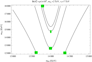
Figure 7: Contour plots of LFVHD as function of $v_{3}$ and $m_{H_{2}}$ in the left (right) panel.

The figure 7 represents some particular regions of the parameter space to get the large values of LFVHD Br$(h^{0}_{1}\rightarrow\mu\tau)$. Especially the values larger than $10^{-5}$ are the maximal values of LFVHD that the 3-3-1LHN can predict when the lower bound of $v_{3}$ is 6 TeV. In addition, the left panel shows the case of $m_{N_{2}}/v_{3}=2$, the parameters satisfying Br$(h^{0}_{1}\rightarrow\mu\tau)\geq 0.5\times 10^{-6}$ is very narrow, implies a very strict relation of $v_{3}$ and $m_{H_{2}}$ if this large amount of the branching ratio is observed. The right panel shows the dependence of Br$(h^{0}_{1}\rightarrow\mu\tau)$ on the Yukawa couplings and $m_{H_{2}}$ with $v_{3}=7$ TeV. Clearly, the maximal peak of LFVHD corresponds to $m_{H_{2}}\simeq 14$ TeV and does not depend on the Yukawa couplings. But the maximal values do, in this case Br$(h^{0}_{1}\rightarrow\mu\tau)\geq 0.5\times 10^{-5}$ if only $m_{N_{2}}\geq 14.5$ TeV. Furthermore, the region having Br$(h^{0}_{1}\rightarrow\mu\tau)\geq 0.5\times 10^{-5}$ opens wider with larger Yukawa couplings.

Finally, we should pay attention to the case satisfying the constraint of universal Higgs fit (108). In the above numerical investigation, we have fixed $\lambda_{1}=1$, which corresponds to $m_{H_{2}}\simeq 2v_{3}\sqrt{\lambda_{1}}=2v_{3}$ satisfying the constraint. It is very interesting that all maximal peaks of LFVHD appearing in the numerical calculations correspond to this relation among $m_{H_{2}},v_{3}$ and $\lambda_{1}$. Therefore the universal Higgs fit confirms more strongly that the 3-3-1LHN predicts the large branching ratios of LFVHD.

V Conclusion

For studying the LFVHD in the 3-3-1LHN model, we have introduced form factors expressing the one-loop contributions corresponding to relevant Feynman diagrams in the unitary gauge. We have checked that the total contribution is finite, all of the divergences appearing in particular diagrams cancel among one to another. Although the above form factors are calculated for the 3-3-1LHN, they can be applied for other 3-3-1 models and in general for many other models beyond the SM with the same class of particles. In numerical investigation the LFVHD in the case of maximal mixing between the first two exotic neutral leptons, we find that the branching ratio Br$(h^{0}_{1}\rightarrow\mu\tau)$ depends the mostly on Yukawa couplings of neutral exotic leptons and the $SU(3)_{L}$ scale $v_{3}$. For small $y^{N}_{ij}\simeq 1$, equivalently $m_{N_{2}}/v_{3}\simeq 0.7$, this branching ratio is always lower than $10^{-6}$, and even that of about $10^{-7}$, the parameter space is very narrow. In contrast, with large Yukwa couplings, for example $y^{N}_{ij}\simeq 2\sqrt{2}$ or $m_{N_{2}}/v_{3}\simeq 2$,the largest LFVHD branching ratio can reach $10^{-5}$ and does not depend on the small values of $m_{N_{1}}$. These largest values do also depend on the charged Higgs masses and the $v_{3}$, thought these seem not as strongly as the Yukawa couplings. The values above $10^{-5}$ can be found in large region of parameter space with small $v_{3}$. With the large $v_{3}$, this region is very small, implying some strict relation between parameters of exotic lepton masses, charged Higgs masses and the $SU(3)_{L}$ scale $v_{3}$. The relation arises from the present of both the custodial symmetry in the Higgs potential and the constraint from the universal fit of the Higgs property observed by LHC. This will give interesting information of the 3-3-1LHN model if the LFVHD branching ratio is discovered by experiments at the value of $10^{-5}$ or larger. Our calculation also indicates that only 3-3-1 models with new heavy leptons, such as newHeavyL , can predict large LFVHD. So when calculating the LFVHD in SUSY versions, the non-SUSY contributions must be included. In contrast, the 3-3-1 models with light leptons newLihgtL give suppressed signals of LFVHD, and the SUSY-contributions in SUSY331 are dominant.

Appendix A Master integrals for one-loop integral calculation

A.1 Master integrals

The calculation in this section relates with one-loop diagrams in the figure 1. We introduce the notations $D_{0}=k^{2}-M_{0}^{2}+i\delta$, $D_{1}=(k-p_{1})^{2}-M_{1}^{2}+i\delta$ and $D_{2}=(k+p_{2})^{2}-M_{2}^{2}+i\delta$, where $\delta$ is infinitesimally a positive real quantity. The scalar integrals are defined as

$$A_{0}(M_{i}) = \frac{\left(2\pi\mu\right)^{4-D}}{i\pi^{2}}\int\frac{d^{D}k}{D_{i}},\hskip 14.22636ptB^{(1)}_{0}\equiv\frac{\left(2\pi\mu\right)^{4-D}}{i\pi^{2}}\int\frac{d^{D}k}{D_{0}D_{1}},$$

$$B^{(2)}_{0} \equiv \frac{\left(2\pi\mu\right)^{4-D}}{i\pi^{2}}\int\frac{d^{D}k}{D_{0}D_{2}},\hskip 14.22636ptB^{(12)}_{0}\equiv\frac{\left(2\pi\mu\right)^{4-D}}{i\pi^{2}}\int\frac{d^{D}k}{D_{1}D_{2}},$$

$$C_{0} \equiv C_{0}(M_{0},M_{1},M_{2})=\frac{1}{i\pi^{2}}\int\frac{d^{4}k}{D_{0}D_{1}D_{2}},$$ (128)

where $i=1,2$. In addition, $D=4-2\epsilon\leq 4$ is the dimension of the integral. The notations $~{}M_{0},~{}M_{1},~{}M_{2}$ are masses of virtual particles in the loops. The momenta satisfy conditions: $p^{2}_{1}=m^{2}_{1},~{}p^{2}_{2}=m^{2}_{2}$, and $(p_{1}+p_{2})^{2}=m^{2}_{h^{0}}$. The tensor integrals are

$$A^{\mu}(p_{i};M_{i}) = \frac{\left(2\pi\mu\right)^{4-D}}{i\pi^{2}}\int\frac{d^{D}k\times k^{\mu}}{D_{i}}=A_{0}(M_{i})p_{i}^{\mu},$$

$$B^{\mu}(p_{i};M_{0},M_{i}) = \frac{\left(2\pi\mu\right)^{4-D}}{i\pi^{2}}\int\frac{d^{D}k\times k^{\mu}}{D_{0}D_{i}}\equiv B^{(i)}_{1}p^{\mu}_{i},$$

$$B^{\mu}(p_{1},p_{2};M_{1},M_{i}) = \frac{\left(2\pi\mu\right)^{4-D}}{i\pi^{2}}\int\frac{d^{D}k\times k^{\mu}}{D_{1}D_{2}}\equiv B^{(12)}_{1}p^{\mu}_{1}+B^{(12)}_{2}p^{\mu}_{2},$$

$$C^{\mu} = C^{\mu}(M_{0},M_{1},M_{2})=\frac{1}{i\pi^{2}}\int\frac{d^{4}k\times k^{\mu}}{D_{0}D_{1}D_{2}}\equiv C_{1}p_{1}^{\mu}+C_{2}p_{2}^{\mu},$$

where $A_{0}$, $B^{(i)}_{0,1}$, $B^{(12)}_{i}$ and $C_{0,1,2}$ are PV- functions. It is well-known that $C_{i}$ is finite while the remains are divergent. We define

$$\Delta_{\epsilon}\equiv\frac{1}{\epsilon}+\ln 4\pi-\gamma_{E}+\ln\frac{\mu^{2}}{m_{h}^{2}},$$ (130)

where $\gamma_{E}$ is the Euler constant and $m_{h}$ is the mass of the neutral Higgs. The divergent parts of the above scalar factors can be determined as

$$\mathrm{Div}[A_{0}(M_{i})] = M_{i}^{2}\Delta_{\epsilon},\hskip 14.22636pt\mathrm{Div}[B^{(i)}_{0}]=\mathrm{Div}[B^{(12)}_{0}]=\Delta_{\epsilon},$$

$$\mathrm{Div}[B^{(1)}_{1}] = \mathrm{Div}[B^{(12)}_{1}]=\frac{1}{2}\Delta_{\epsilon},\hskip 14.22636pt\mathrm{Div}[B^{(2)}_{1}]=\mathrm{Div}[B^{(12)}_{2}]=-\frac{1}{2}\Delta_{\epsilon}.$$ (131)

We remind that the finite parts of the PV-functions such as B-functions depend on the scale of $\mu$ parameter with the same coefficient of the divergent parts.

The analytic formulas of the above PV-functions are:

$$A_{0}(M)=M^{2}\left(\Delta_{\epsilon}+\ln\frac{m_{h}^{2}-i\delta}{M^{2}-i\delta}+1\right)\equiv M^{2}\Delta_{\epsilon}+a_{0}(M),$$ (132)

$$B^{(i)}_{0,1}=\mathrm{Div}[B^{(i)}_{0,1}]+b^{(i)}_{0,1},\hskip 14.22636ptB^{(12)}_{0,1,2}=\mathrm{Div}[B^{(12)}_{0,1,2}]+b^{(12)}_{0,1,2},$$ (133)

where

$$b^{(i)}_{0} = \ln(m_{h}^{2}-i\delta)-\int^{1}_{0}dx\ln\left[x^{2}p_{i}^{2}-x(p_{i}^{2}+M^{2}_{0}-M^{2}_{i})+M_{0}^{2}-i\delta\right],$$

$$b^{(12)}_{0} = \ln(m_{h}^{2}-i\delta)-\int^{1}_{0}dx\ln\left[m_{h}^{2}x^{2}-x(m_{h}^{2}+M^{2}_{1}-M^{2}_{2})+M_{1}^{2}-i\delta\right].$$

The $b^{(1)}_{0}$ can be found in a very simple form in the limit $p_{i}^{2}\rightarrow 0$. The $b_{0}^{(12)}$ is determined by

$$b_{0}^{(12)}=-\sum_{k=1}^{2}\int^{1}_{0}dx\ln(x-x_{k}),$$ (135)

where $x_{k},~{}(k=1,2)$ are solutions of the equation

$$x^{2}-\left(\frac{m_{h}^{2}-M_{1}^{2}+M_{2}^{2}}{m_{h}^{2}}\right)x+\frac{M_{2}^{2}-i\delta}{m_{h}^{2}}=0.$$ (136)

The final expression of $b^{(12)}_{0}$ is

$$b_{0}^{(12)} = \ln\frac{m_{h}^{2}-i\delta}{M_{1}^{2}-i\delta}+2+\sum_{k=1}^{2}x_{k}\ln\left(1-\frac{1}{x_{k}}\right).$$ (137)

The $B^{i}_{1},~{}B^{(12)}_{i}$ are calculated through the $B_{0}$ and $A_{0}$ functions, namely

$$B^{(i)}_{1} = \frac{(-1)^{i-1}}{2m^{2}_{i}}\left[A_{0}(M_{i})-A_{0}(M_{0})+B^{(i)}_{0}(M_{0}^{2}-M_{i}^{2}+m_{i}^{2})\right],$$

$$B^{(12)}_{i} = \frac{1}{2m^{2}_{h}}\left[A_{0}(M_{1})-A_{0}(M_{2})+B^{(12)}_{0}\left(M_{2}^{2}-M_{1}^{2}+(-1)^{i-1}m_{h}^{2}\right)\right].$$

The $C_{i}$ functions can be found through the equation

$$\left(\begin{array}[]{cc}2m^{2}_{1}&m^{2}_{h}-m_{1}^{2}-m_{2}^{2}\\ m^{2}_{h}-m_{1}^{2}-m_{2}^{2}&2m_{2}^{2}\\ \end{array}\right)\left(\begin{array}[]{c}C_{1}\\ C_{2}\\ \end{array}\right)$$ (143)

$$= \left(\begin{array}[]{c}B^{(12)}_{0}-B^{(2)}_{0}+(M_{0}^{2}-M_{1}^{2}+m_{1}^{2})C_{0}\\ -\left[B^{(12)}_{0}-B^{(1)}_{0}+(M_{0}^{2}-M_{2}^{2}+m_{2}^{2})C_{0}\right]\\ \end{array}\right).$$ (146)

The $C_{0}$ function was generally calculated in Hooft , a more explicit explanation was given in Ninhthes . In the limit $p_{1}^{2},p_{2}^{2}\rightarrow 0$, we get the following expression

$$C_{0} = -\int^{1}_{0}dx\int^{1-x}_{0}\frac{dy}{(1-x-y)M_{0}^{2}+xM_{1}^{2}+yM_{2}^{2}-xym_{h}^{2}-i\delta}$$ (147)

$$= \frac{1}{m_{h}^{2}}\int^{1}_{0}\frac{dx}{x-x_{0}}$$

$$\times \left[\ln\frac{m_{h}^{2}-i\delta^{\prime}}{M_{1}^{2}-M_{0}^{2}-i\delta^{\prime}}+\ln(x-x_{1})+\ln(x-x_{2})-\ln(x-x_{3})\right]$$

$$= \frac{1}{m_{h}^{2}}\ln\frac{m_{h}^{2}-i\delta^{\prime}}{M_{1}^{2}-M_{0}^{2}-i\delta^{\prime}}\times\ln\left(1-\frac{1}{x_{0}}\right)$$

$$+ \frac{1}{m_{h}^{2}}\int^{1}_{0}\frac{dx}{x-x_{0}}\left[\ln(x-x_{1})+\ln(x-x_{2})-\ln(x-x_{3})\right],$$

where both $\delta$ and $\delta^{\prime}$ are positive and extremely small, $x_{0}$ and $x_{3}$ are defined as

$$x_{0}=\frac{M_{2}^{2}-M_{0}^{2}}{m_{h}^{2}},\hskip 14.22636ptx_{3}=\frac{-M_{0}^{2}+i\delta}{M_{1}^{2}-M_{0}^{2}},$$ (148)

and $x_{1},x_{2}$ are solutions of the equation (136). The limit of $p_{1}^{2},p_{2}^{2}=0$ will be used in our work, even when the loops contain active neutrinos with masses extremely smaller than these quantities, because of the appearance of heavy virtual particles. The explanation is as follows. The denominator in the first line of (147) has the general form of $D=(1-x-y)M_{0}^{2}+xM_{1}^{2}+yM_{2}^{2}-xym_{h}^{2}-i\delta-(1-x-y)\left[xm_{1}^{2}+ym_{2}^{2}\right]$. Our calculation relates to the two following cases:

• Only $M_{0}$ is the mass of the active neutrino, $M_{0}\ll M_{1},M_{2}$. We have $D=(1-x-y)M_{0}^{2}+xM_{1}^{2}\left[1-(1-x-y)m_{1}^{2}/M_{1}^{2}\right]+yM_{2}^{2}\left[1-(1-x-y)m_{2}^{2}/M_{2}^{2}\right]-xym_{h}^{2}-i\delta\simeq(1-x-y)M_{0}^{2}+xM_{1}^{2}+yM_{2}^{2}-xym_{h}^{2}-i\delta$.

• $M_{1}=M_{2}$ is the mass of the neutrino: $M_{1}=M_{2}\ll M_{0}$. Then we have $D=(1-x-y)M_{0}^{2}\left[1-(xm_{1}^{2}+ym_{2}^{2})/M_{0}^{2}\right]+xM_{1}^{2}+yM_{2}^{2}-xym_{h}^{2}-i\delta\simeq(1-x-y)M_{0}^{2}+xM_{1}^{2}+yM_{2}^{2}-xym_{h}^{2}-i\delta$.

We use the following result given in Hooft

$$R(x_{0},x_{i}) \equiv \int_{0}^{1}\frac{dx}{x-x_{0}}\left[\ln(x-x_{i})-\ln(x_{0}-x_{i})\right]$$ (149)

$$= Li_{2}(\frac{x_{0}}{x_{0}-x_{i}})-Li_{2}(\frac{x_{0}-1}{x_{0}-x_{i}}),$$

where $i=1,2,3$ and $Li_{2}(z)$ is the di-logarithm defined by

$$Li_{2}(z)\equiv\int_{0}^{1}-\frac{dt}{t}\ln(1-tz).$$

We also use the real values of $x_{0}$ to give the result $\eta(-x_{i},\frac{1}{x_{0}-x_{i}})\ln\frac{x_{0}}{x_{0}-x_{i}}=\eta(1-x_{i},\frac{1}{x_{0}-x_{i}})\ln\frac{x_{0}-1}{x_{0}-x_{i}}=0$ for any complex $x_{i}$. Now we introduce the function

$$R_{0}(x_{0},x_{i})\equiv Li_{2}(\frac{x_{0}}{x_{0}-x_{i}})-Li_{2}(\frac{x_{0}-1}{x_{0}-x_{i}}),$$ (150)

leading to

$$\int_{0}^{1}\frac{dx\ln(x-x_{i})}{x-x_{0}}=R_{0}(x_{0},x_{i})+\ln\left(1-\frac{1}{x_{0}}\right)\ln(x_{0}-x_{i}).$$ (151)

Using the following equalities

$$\ln(AB-i\delta)=\ln(A-i\delta^{\prime})+\ln(B-i\delta/A)$$

with any real $A,B$, $\delta,\delta^{\prime}$ positive real and extremely small; and

$$x_{1}x_{2}=\frac{m^{2}_{h}-M_{1}^{2}+M_{2}^{2}}{m_{h}^{2}},\hskip 14.22636ptx_{1}x_{2}=\frac{M_{2}^{2}-i\delta}{m^{2}_{h}},$$

we can prove that

$$\ln\frac{m_{h}^{2}-i\delta^{\prime}}{M_{1}^{2}-M_{0}^{2}-i\delta^{\prime}}+\ln(x_{0}-x_{1})+\ln(x_{0}-x_{2})-\ln(x_{0}-x_{3})=0.$$

This results the very simple expression of $C_{0}$ function

$$C_{0}=\frac{1}{m_{h}^{2}}\left[R_{0}(x_{0},x_{1})+R_{0}(x_{0},x_{2})-R_{0}(x_{0},x_{3})\right],$$ (152)

where $x_{1,2}$ are solutions of the equation (136), and $x_{0,3}$ are given in (148). This result is consistent with that discussed on bardin .

For simplicity in calculation we will also use other approximations of PV-functions where $p_{1}^{2},p_{2}^{2}\rightarrow 0$, namely

$$a_{0}(M) = M^{2}\left(1+\ln\frac{m_{h}^{2}-i\delta}{M^{2}-i\delta}\right),\hskip 14.22636ptb^{(i)}_{0}=1-\ln\frac{M_{i}^{2}}{m_{h}^{2}}+\frac{M_{0}^{2}}{M_{0}^{2}-M_{i}^{2}}\ln\frac{M_{i}^{2}}{M_{0}^{2}},$$

$$b^{(1)}_{1} = -\frac{1}{2}\ln\frac{M_{1}^{2}}{m_{h}^{2}}-\frac{M_{0}^{4}}{2(M_{0}^{2}-M_{1}^{2})^{2}}\ln\frac{M_{0}^{2}}{M_{1}^{2}}+\frac{(M_{0}^{2}-M^{2}_{1})(3M_{0}^{2}-M_{1}^{2})}{4(M_{0}^{2}-M_{1}^{2})^{2}},$$

$$b^{(2)}_{1} = \frac{1}{2}\ln\frac{M_{2}^{2}}{m_{h}^{2}}+\frac{M_{0}^{4}}{2(M_{0}^{2}-M_{2}^{2})^{2}}\ln\frac{M_{0}^{2}}{M_{2}^{2}}-\frac{(M_{0}^{2}-M^{2}_{2})(3M_{0}^{2}-M_{2}^{2})}{4(M_{0}^{2}-M_{2}^{2})^{2}},$$

$$b^{(12)}_{0} = \ln\frac{m_{h}^{2}-i\delta}{M_{1}^{2}-i\delta}+2+\sum_{k=1}^{2}x_{k}\ln\left(1-\frac{1}{x_{k}}\right),$$

where $x_{k}$ is the two solutions of the equation (136),

$$b^{(12)}_{i} = \frac{1}{2m^{2}_{h}}\left[M_{1}^{2}\left(1+\ln\frac{m_{h}^{2}}{M_{1}^{2}}\right)-M_{2}^{2}\left(1+\ln\frac{m_{h}^{2}}{M_{2}^{2}}\right)\right]$$

$$+\frac{b^{(12)}_{0}}{2m^{2}_{h}}\left[M_{2}^{2}-M_{1}^{2}+(-1)^{i-1}m_{h}^{2}\right],$$

$$C_{1} = \frac{1}{m_{h}^{2}}\left[b^{(1)}_{0}-b_{0}^{(12)}+(M_{2}^{2}-M_{0}^{2})C_{0}\right],$$

$$C_{2} = -\frac{1}{m_{h}^{2}}\left[b^{(2)}_{0}-b_{0}^{(12)}+(M_{1}^{2}-M_{0}^{2})C_{0}\right].$$

Appendix B Calculations the one loop contributions

In the first part of this section we will calculate in details the contributions of particular contributions of diagrams shown in the figure 1 which involve with exotic neutral lepton $N_{a}$, $a=1,2,3$. From this we can derive the general functions expressing the contributions of particular diagrams.

B.1 Amplitudes

It is needed to remind that the amplitude will be expressed in terms of the PV-functions, so the integral will be written as

$$\int\frac{d^{4}k}{(2\pi)^{4}}\rightarrow\frac{i}{16\pi^{2}}\times\frac{(2\pi\mu)^{4-D}}{i\pi^{2}}\int d^{4}k,$$

where $\mu$ is a parameter with dimension of mass. This step will be omitted in the below calculation, the final results are simply corrected by adding the factor $i/16\pi^{2}$. As an example in the calculation of contribution from the first diagram, we will point out a class of divergences that automatically vanish by the GIM mechanism. More explicitly for any terms which do not depend on the masses of virtual leptons, they will vanish because of the appearance of the factor $\sum_{a}V^{L}_{1a}V^{L*}_{2a}=0$.

The contribution from diagram 1a) is:

$$i\mathcal{M}_{(a)}^{FVV} = \sum_{a}\int\frac{d^{4}k}{(2\pi)^{4}}\times\bar{u}_{1}\frac{ig}{\sqrt{2}}V_{1a}\gamma^{\mu}P_{L}\frac{1(/\!\!\!k+m_{a})}{D_{0}}\frac{ig}{\sqrt{2}}V^{*}_{2a}\gamma^{\nu}P_{L}v_{2}$$ (153)

$$\times\left[\frac{igm_{V}}{\sqrt{2}}\left(-c_{\alpha}s_{\theta}+\sqrt{2}s_{\alpha}c_{\theta}\right)\right]\frac{-i}{D_{1}}$$

$$\times\left[g_{\mu\alpha}-\frac{(k-p_{1})_{\mu}(k-p_{1})_{\alpha}}{m_{V}^{2}}\right]\frac{-i}{D_{2}}\left[g_{\nu\beta}-\frac{(k+p_{2})_{\nu}(k+p_{2})_{\beta}}{m_{V}^{2}}\right]$$

$$= \sum_{a}V_{1a}V^{*}_{2a}(-1)\frac{g^{3}m_{V}}{2\sqrt{2}}\left(-c_{\alpha}s_{\theta}+\sqrt{2}s_{\alpha}c_{\theta}\right)\times\int\frac{d^{4}k}{(2\pi)^{4}}\frac{\bar{u}_{1}\gamma^{\mu}/\!\!\!k\gamma^{\nu}P_{L}v_{2}}{D_{0}D_{1}D_{2}}$$

$$\times g^{\alpha\beta}\left[g_{\mu\alpha}-\frac{(k-p_{1})_{\mu}(k-p_{1})_{\alpha}}{m^{2}_{V}}\right]\left[g_{\beta\nu}-\frac{(k+p_{2})_{\nu}(k+p_{1})_{\beta}}{m^{2}_{V}}\right]$$

$$\equiv \sum_{a}V_{1a}V^{*}_{2a}(-1)\frac{g^{3}m_{V}}{2\sqrt{2}}\left(-c_{\alpha}s_{\theta}+\sqrt{2}s_{\alpha}c_{\theta}\right)\left[P_{1}+P_{2}+P_{3}\right],$$

where

$$P_{1} = \int\frac{d^{4}k}{(2\pi)^{4}}\frac{\bar{u}_{1}\gamma^{\mu}/\!\!\!k\gamma^{\nu}P_{L}v_{2}}{D_{0}D_{1}D_{2}}g_{\mu\nu}=\int\frac{d^{4}k}{(2\pi)^{4}}\frac{(2-d)\bar{u}_{1}/\!\!\!kP_{L}v_{2}}{D_{0}D_{1}D_{2}}$$ (154)

$$= \bar{u}_{1}P_{L}v_{2}\times m_{1}(-2C_{1})+\bar{u}_{1}P_{L}v_{2}\times m_{2}(2C_{2}),$$

We can see that $P_{1}$ does not contain any divergent terms. The formula of $P_{2}$ is

$$P_{2} = \frac{-1}{m^{2}_{V}}\int\frac{d^{4}k}{(2\pi)^{4}}\frac{\bar{u}_{1}\gamma^{\mu}/\!\!\!k\gamma^{\nu}P_{L}v_{2}}{D_{0}D_{1}D_{2}}\left[(k+p_{2})_{\mu}(k+p_{2})_{\nu}+(k-p_{1})_{\mu}(k-p_{1})_{\nu}\right]$$ (155)

$$= \frac{-1}{m^{2}_{V}}\int\frac{d^{4}k}{(2\pi)^{4}}\left[\frac{\bar{u}_{1}(D_{0}+m^{2}_{a})(/\!\!\!k+2/\!\!\!p_{2})P_{L}v_{2}+\bar{u}_{1}/\!\!\!p_{2}/\!\!\!k/\!\!\!p_{2}P_{L}v_{2}}{D_{0}D_{1}D_{2}}\right.$$

$$+\left.\frac{\bar{u}_{1}(D_{0}+m^{2}_{a})(/\!\!\!k-2/\!\!\!p_{1})P_{L}v_{2}+\bar{u}_{1}/\!\!\!p_{1}/\!\!\!k/\!\!\!p_{1}P_{L}v_{2}}{D_{0}D_{1}D_{2}}\right]$$

$$= \frac{-1}{m^{2}_{V}}\left\{\frac{}{}\bar{u}_{1}P_{L}v_{2}\times m_{1}\left[\frac{}{}2B^{(12)}_{1}(m_{V})-2B^{(12)}_{0}(m_{V})\right.\right.$$

$$\left.\left.-2m_{a}^{2}C_{0}+(2m^{2}_{a}+m^{2}_{1}-m_{2}^{2})C_{1}+(m^{2}_{H_{0}}-m_{1}^{2}-m_{2}^{2})C_{2}\dfrac{}{}\right]\right.$$

$$\left.+\bar{u}_{1}P_{R}v_{2}\times m_{2}\left[\frac{}{}-2B^{(12)}_{2}(m_{V})-2B^{(12)}_{0}(m_{V})\right.\right.$$

$$\left.\left.-2m_{a}^{2}C_{0}-(2m^{2}_{a}-m^{2}_{1}+m^{2}_{2})C_{2}-(m^{2}_{H_{0}}-m_{1}^{2}-m^{2}_{2})C_{1}\frac{}{}\right]\right\}.$$

We can see that the terms like $B^{(12)}_{1}(m_{V}),~{}B^{(12)}_{1}(m_{V})$ and $B^{(12)}_{0}(m_{V})$ do contain divergences but theydo not depend on $m_{a}$ in the loop. Hence these terms will exactly cancel by the GIM mechanism. All of the other are finite.

The contribution from $P_{3}$ is

$$P_{3} = \frac{1}{m^{4}_{V}}\int\frac{d^{4}k}{(2\pi)^{4}}\times\frac{\bar{u}_{1}\gamma^{\mu}/\!\!\!k\gamma^{\nu}P_{L}v_{2}}{D_{0}D_{1}D_{2}}\left[(k-p_{1}).(k+p_{2})(k-p_{1})_{\mu}(k+p_{2})_{\nu}\right]$$ (156)

$$= \frac{1}{2m^{4}_{V}}\int\frac{d^{4}k}{(2\pi)^{4}}\times\left[\frac{\bar{u}_{1}[D_{1}+D_{2}+2m_{V}^{2}-m^{2}_{H_{0}}](D_{0}+m_{a}^{2})(/\!\!\!k+/\!\!\!p_{2}-/\!\!\!p_{1})P_{L}v_{2}}{D_{0}D_{1}D_{2}}\right.$$

$$\left.+m_{1}m_{2}\frac{\bar{u}_{1}[D_{1}+D_{2}+2m_{V}^{2}-m^{2}_{H_{0}}]/\!\!\!kP_{L}v_{2}}{D_{0}D_{1}D_{2}}\right]$$

$$= \frac{1}{2m^{4}_{V}}\left\{\frac{}{}\bar{u}_{1}P_{L}v_{2}\times m_{1}\left[-A_{0}(m_{V})+(2m_{V}^{2}-m^{2}_{H_{0}})\left(B^{(12)}_{1}(m_{V})-B^{(12)}_{0}(m_{V})\right)\right.\right.$$

$$\left.\left.-m_{2}^{2}B^{(2)}_{1}+\mathbf{m^{2}_{a}\left(B^{(1)}_{1}-B^{(1)}_{0}-B^{(2)}_{0}\right)}\right.\right.$$

$$\left.\left.+(2m_{V}^{2}-m^{2}_{H_{0}})\left(\frac{}{}m^{2}_{a}(C_{1}-C_{0})-m_{2}^{2}C_{2}\right)\right]\right.$$

$$\left.+\bar{u}_{1}P_{R}v_{2}\times m_{2}\left[-A_{0}(m_{V})+(2m_{V}^{2}-m^{2}_{H_{0}})\left(-B^{(12)}_{2}(m_{V})-B^{(12)}_{0}(m_{V})\right)\right.\right.$$

$$\left.\left.+m_{1}^{2}B^{(1)}_{1}+\mathbf{m_{a}^{2}\left(-B^{(1)}_{0}-B^{(2)}_{0}-B^{(2)}_{1}\right)}\right.\right.$$

$$\left.\left.+(2m_{V}^{2}-m^{2}_{H_{0}})\left(\frac{}{}m_{1}^{2}C_{1}-m^{2}_{a}(C_{0}+C_{2})\right)\right]\right\}.$$

Again all terms in the first and third lines do not contribute to the amplitude. But the four terms $m_{2}^{2}B^{(2)}_{1},$ $m_{1}^{2}B^{(1)}_{1}$, $m^{2}_{a}\left(B^{(1)}_{1}-B^{(1)}_{0}-B^{(2)}_{0}\right)$ and $m_{a}^{2}\left(-B^{(1)}_{0}-B^{(2)}_{0}-B^{(2)}_{1}\right)$ do contain divergences. The first two terms have divergent parts having the corresponding forms of $(-m_{2}^{2}\Delta_{\epsilon})$ and $m_{1}^{2}\Delta_{\epsilon}$, which do not depend on the masses $m_{a}$ of the virtual leptons. Hence they also vanish by the GIM mechanism. The finite parts of these terms still contribute to the amplitude. The remain two terms include the most dangerous divergent parts. They have factors $m_{a}^{2}$ which can not cancel by the GIM mechanism. We remark them by the bold and will prove later that they finally vanish after summing all diagrams. From now on we can exclude all terms that do not depend on the masses of virtual leptons.

Based on definition $\mathcal{M}=-\left(E^{FVV}_{L}\overline{u_{1}}P_{L}v_{2}+E^{FVV}_{R}\overline{u_{1}}P_{R}v_{2}\right)$, the expression of the total contribution from the diagram 1a) is simply

$$\mathcal{M}_{(a)}^{FVV}=\frac{-g^{3}}{32\pi^{2}\sqrt{2}}\left(-c_{\alpha}s_{\theta}+\sqrt{2}s_{\alpha}c_{\theta}\right)\sum_{a}V_{1a}V^{*}_{2a}\left[\left(\overline{u_{1}}P_{L}v_{2}\right)E^{FVV}_{L}+\left(\overline{u_{1}}P_{R}v_{2}\right)E^{FVV}_{R}\right],$$ (157)

where $E^{FVV}_{L,R}$ is defined in (4) and (5). Here we have added a factor of $\frac{i}{16\pi^{2}}$. All terms being independent on $m_{a}$ will cancel by the factor $\sum_{a}V_{1a}V^{*}_{2a}$. If we assume all other divergences cancel among themselves after summing all of the diagrams, the analytic formulas of $E^{FVV}_{L}$ and $E^{FVV}_{R}$ can be written in terms of the finite parts of PV-functions, i.e $b^{(i)}_{0},b^{(12)}_{0},b^{i}_{1},\;b^{(12)}_{i}$ and $C_{0,1,2}$. The following calculation for the remain diagrams will be done the same as what we have done above. We trace the divergence of each diagram in the bold text.

The contribution from diagram 1b) is:

$$i\mathcal{M}^{FVH}_{(b)} = \sum_{a}\int\frac{d^{4}k}{(2\pi)^{4}}$$ (158)

$$\times \bar{u}_{1}\frac{ig}{\sqrt{2}}V_{1a}\gamma^{\mu}P_{L}\frac{i(/\!\!\!k+m_{a})}{D_{0}}(-i\sqrt{2}V_{2a}^{*})\left(\frac{m_{2}}{v_{1}}a_{1}P_{R}+\frac{m_{a}}{v_{3}}a_{3}P_{L}\right)v_{2}$$

$$\times\frac{ig}{2\sqrt{2}}(-k-2p_{2}-p_{1})^{\alpha}\frac{i}{D_{2}}\frac{-i}{D_{1}}\left[g_{\mu\alpha}-\frac{(k-p_{1})_{\mu}(k-p_{1})_{\alpha}}{m^{2}_{V}}\right]$$

$$= \sum_{a}V_{1a}V^{*}_{2a}\frac{g^{2}}{2\sqrt{2}}(c_{\alpha}c_{\theta}+\sqrt{2}s_{\alpha}s_{\theta})\int$$

$$\times\frac{d^{4}k}{(2\pi)^{4}}\times\frac{\frac{m_{2}}{v_{1}}a_{1}\bar{u}_{1}\gamma^{\mu}/\!\!\!kP_{R}v_{2}+\frac{m^{2}_{a}}{v_{2}}a_{2}\bar{u}_{1}\gamma^{\mu}P_{L}v_{2}}{D_{0}D_{1}D_{2}}$$

$$\times\left[(k+2p_{2}+p_{1})_{\mu}-\frac{(k+2p_{2}+p_{1}).(k-p_{1})(k-p_{1})_{\mu}}{m_{V}^{2}}\right]$$

$$= \sum_{a}V_{1a}V^{*}_{2a}\left[\frac{g^{2}}{2\sqrt{2}}(c_{\alpha}c_{\theta}+\sqrt{2}s_{\alpha}s_{\theta})\right]$$

$$\times\left\{\frac{}{}\bar{u}_{1}P_{L}v_{2}\times\left[\frac{}{}\framebox{$\bf\frac{-m_{1}}{m^{2}_{V}}\frac{m^{2}_{a}}{v_{3}}a_{3}\left(B_{1}^{(1)}-B^{(1)}_{0}\right)$}\right.\right.$$

$$\left.\left.+\frac{m^{2}_{a}}{v_{3}}a_{3}\times m_{1}\left(C_{0}+C_{1}+\frac{(m^{2}_{H_{A}}-m^{2}_{H_{0}})}{m_{V}^{2}}(C_{0}-C_{1})\right)\right.\right.$$

$$\left.\left.+\frac{m_{2}}{v_{1}}a_{1}\times m_{1}m_{2}\left(2C_{1}-C_{2}-\frac{m^{2}_{H_{A}}-m^{2}_{H_{0}}}{m_{V}^{2}}C_{2}\right)\right]\right.$$

$$\left.+\bar{u}_{1}P_{R}v_{2}\times\left[\dfrac{-1}{m_{V}^{2}}\frac{m_{2}}{v_{1}}a_{1}\left(A_{0}(m_{V})+(m^{2}_{H_{A}}-m^{2}_{H_{0}})B_{0}^{(12)}\right)\right.\right.$$

$$\left.\left.+\frac{m_{2}}{v_{1}}a_{1}B_{0}^{(12)}+\frac{m_{1}^{2}}{m_{V}^{2}}\frac{m_{2}}{v_{1}}a_{1}B_{1}^{(1)}-\framebox{$\bf\dfrac{m_{a}^{2}}{m_{V}^{2}}\dfrac{m_{2}}{v_{1}}a_{1}B^{(1)}_{0}(m_{a},m_{V})$}\right.\right.$$

$$\left.\left.+\frac{m_{2}}{v_{1}}a_{1}\left(m_{a}^{2}C_{0}-m^{2}_{1}C_{1}+2m_{2}^{2}C_{2}+2(m^{2}_{H_{0}}-m_{2}^{2})C_{1}\right.\right.\right.$$

$$-\left.\left.\left.\frac{(m^{2}_{H_{A}}-m^{2}_{H_{0}})}{m_{V}^{2}}\left(m_{a}^{2}C_{0}-m_{1}^{2}C_{1}\right)\right)\right.\right.$$

$$\left.\left.+\frac{m_{a}^{2}}{v_{3}}a_{3}\times m_{2}\left(-2C_{0}-C_{2}+\frac{(m^{2}_{H_{A}}-m^{2}_{H_{0}})}{m_{V}^{2}}C_{2}\right)\frac{}{}\right]\right\}.$$

The contribution to the total amplitude is

$$\mathcal{M}_{(b)}^{FVH}=\frac{g^{2}}{32\pi^{2}\sqrt{2}}\left(c_{\alpha}c_{\theta}+\sqrt{2}s_{\alpha}s_{\theta}\right)\sum_{a}V_{1a}V^{*}_{2a}\left[\left(\overline{u_{1}}P_{L}v_{2}\right)E^{FVH}_{L}+\left(\overline{u_{1}}P_{R}v_{2}\right)E^{FVH}_{R}\right],$$ (159)

The contribution from diagram 1c) is:

$$i\mathcal{M}^{FHV}_{(c)} = \sum_{a}\int\frac{d^{4}k}{(2\pi)^{4}}\times\bar{u}_{1}(-i\sqrt{2}V_{1a})\left(\frac{m_{1}}{v_{1}}a_{1}P_{L}+\frac{m_{a}}{v_{3}}a_{3}P_{R}\right)$$ (160)

$$\times\frac{i(/\!\!\!k+m_{a})}{D_{0}}\frac{ig}{\sqrt{2}}V^{*}_{2a}\gamma^{\mu}P_{L}v_{2}\times\frac{ig}{2\sqrt{2}}(c_{\alpha}c_{\theta}+\sqrt{2}s_{\alpha}s_{\theta})(-k+p_{2}+2p_{1})^{\alpha}$$

$$\times \frac{i}{D_{1}}\frac{-i}{D_{2}}\times\left[g_{\mu\alpha}-\frac{(k+p_{2})_{\mu}(k+p_{2})_{\alpha}}{m^{2}_{V}}\right]$$

$$= \sum_{a}V_{1a}V^{*}_{2a}\frac{g^{2}}{2\sqrt{2}}(c_{\alpha}c_{\theta}+\sqrt{2}s_{\alpha}s_{\theta})\int\frac{d^{4}k}{(2\pi)^{4}}$$

$$\times\left[\frac{m_{1}}{v_{1}}a_{1}\frac{\bar{u}_{1}\gamma^{\mu}/\!\!\!kP_{L}v_{2}}{D_{0}D_{1}D_{2}}+\frac{m^{2}_{a}}{v_{3}}a_{3}\frac{\bar{u}_{1}\gamma^{\mu}P_{L}v_{2}}{D_{0}D_{1}D_{2}}\right]$$

$$\times\left[(k-p_{2}-2p_{1})_{\mu}-\frac{(k-p_{2}-2p_{1}).(k+p_{2})(k+p_{2})_{\mu}}{m_{V}^{2}}\right]$$

$$= \sum_{a}V_{1a}V^{*}_{2a}\left[\frac{g^{2}}{2\sqrt{2}}(c_{\alpha}c_{\theta}+\sqrt{2}s_{\alpha}s_{\theta})\right]V_{1a}V^{*}_{2a}$$

$$\times\left\{\frac{}{}\bar{u}_{1}P_{L}v_{2}\times\left[\frac{-1}{m_{V}^{2}}\frac{m_{1}}{v_{1}}a_{1}\left(A_{0}(m_{V})+(m^{2}_{H_{A}}-m^{2}_{H_{0}})B_{0}^{(12)}\right)\right.\right.$$

$$\left.\left.+\frac{m_{1}}{v_{1}}a_{1}B_{0}^{(12)}(m_{V},m_{H_{A}})-\frac{m_{2}^{2}}{m_{V}^{2}}\frac{m_{1}}{v_{1}}a_{1}B^{(2)}_{1}(m_{a},m_{V})\right.\right.$$

$$- \left.\left.\framebox{$\bf\dfrac{m_{a}^{2}}{m_{V}^{2}}\dfrac{m_{1}}{v_{1}}a_{1}B_{0}^{(2)}(m_{a},m_{V})$}\right.\right.$$

$$\left.\left.+\frac{m_{1}}{v_{1}}a_{1}\left(\frac{}{}m_{a}^{2}C_{0}-2m_{1}^{2}C_{1}+m_{2}^{2}C_{2}-2(m^{2}_{H_{0}}-m_{1}^{2})C_{2}\right.\right.\right.$$

$$\left.\left.\left.-\frac{(m^{2}_{H_{A}}-m^{2}_{H_{0}})}{m_{V}^{2}}(m_{2}^{2}C_{2}+m_{a}^{2}C_{0})\right)\right.\right.$$

$$\left.\left.+m_{1}\frac{m_{a}^{2}}{v_{3}}a_{3}\left(-2C_{0}+C_{1}-\frac{(m^{2}_{H_{A}}-m^{2}_{H_{0}})}{m_{V}^{2}}C_{1}\right)\right]\right.$$

$$\left.+\bar{u}_{1}P_{R}v_{2}\left[\frac{}{}\framebox{$\bf\dfrac{m_{2}}{m_{V}^{2}}\dfrac{m_{a}^{2}}{v_{3}}a_{3}\left(B_{1}^{(2)}+B_{0}^{(2)}\right)$}\right.\right.$$

$$\left.\left.+m_{1}m_{2}\frac{m_{1}}{v_{1}}a_{1}\left(C_{1}-2C_{2}+\frac{(m^{2}_{H_{A}}-m^{2}_{H_{0}})}{m_{V}^{2}}C_{1}\right)\right.\right.$$

$$\left.\left.+m_{2}\frac{m_{a}^{2}}{v_{3}}a_{3}\left(C_{0}-C_{2}+\frac{(m^{2}_{H_{A}}-m^{2}_{H_{0}})}{m_{V}^{2}}(C_{0}+C_{2})\right)\frac{}{}\right]\right\}.$$

The contribution to the total amplitude is

$$\mathcal{M}_{(c)}^{FHV}=\frac{g^{2}}{32\pi^{2}\sqrt{2}}\left(c_{\alpha}c_{\theta}+\sqrt{2}s_{\alpha}s_{\theta}\right)\sum_{a}V_{1a}V^{*}_{2a}\left[\left(\overline{u_{1}}P_{L}v_{2}\right)E^{FHV}_{L}+\left(\overline{u_{1}}P_{R}v_{2}\right)E^{FHV}_{R}\right].$$ (161)

The contribution from diagram 1d) is:

$$i\mathcal{M}^{FHH}_{(d)} = \sum_{a}\int\frac{d^{4}k}{(2\pi)^{4}}\times(-iv_{3}\lambda_{h^{0}H_{1}H_{1}})\frac{i}{D_{1}}\frac{i}{D_{2}}\times\bar{u}_{1}(-i\sqrt{2}V_{1a})$$ (162)

$$\times \left(\frac{m_{1}}{v_{1}}a_{1}P_{L}+\frac{m_{a}}{v_{3}}a_{3}P_{R}\right)\frac{i(/\!\!\!k+m_{a})}{D_{0}}(-i\sqrt{2}V^{*}_{2a})\left(\frac{m_{2}}{v_{1}}a_{1}P_{R}+\frac{m_{a}}{v_{3}}a_{3}P_{L}\right)v_{2}$$

$$= \sum_{a}v_{3}\lambda_{h^{0}H_{1}H_{1}}V_{1a}V^{*}_{2a}\int\dfrac{d^{4}k}{(2\pi)^{4}}$$

$$\times \frac{\bar{u}_{1}\left(\frac{m_{1}}{v_{1}}a_{1}P_{L}+\frac{m_{a}}{v_{3}}a_{3}P_{R}\right)(/\!\!\!k+m_{a})\left(\frac{m_{2}}{v_{1}}a_{1}P_{R}+\frac{m_{a}}{v_{3}}a_{3}P_{L}\right)v_{2}}{D_{0}D_{1}D_{2}}$$

$$= \sum_{a}v_{3}\lambda_{h^{0}H_{1}H_{1}}V_{1a}V^{*}_{2a}\int\frac{d^{4}k}{(2\pi)^{4}}$$

$$\times \left[\dfrac{m_{1}m_{2}}{v^{2}_{1}}a_{1}^{2}\dfrac{\bar{u}_{1}/\!\!\!kP_{R}v_{2}}{D_{0}D_{1}D_{2}}+\dfrac{m_{1}m^{2}_{a}}{v_{1}v_{3}}a_{1}a_{3}\frac{\bar{u}_{1}P_{L}v_{2}}{D_{0}D_{1}D_{2}}\right.$$

$$\left.+\frac{m^{2}_{a}}{v^{2}_{3}}a_{3}^{2}\frac{\bar{u}_{1}/\!\!\!kP_{L}v_{2}}{D_{0}D_{1}D_{2}}+\frac{m_{2}m^{2}_{a}}{v_{1}v_{3}}a_{1}a_{3}\frac{\bar{u}_{1}P_{R}v_{2}}{D_{0}D_{1}D_{2}}\right]$$

$$= \sum_{a}v_{3}\lambda_{h^{0}H_{1}H_{1}}V_{1a}V^{*}_{2a}$$

$$\times \left\{\bar{u}_{1}P_{L}v_{2}\times m_{1}\left[\frac{m_{a}^{2}}{v_{1}v_{3}}a_{1}a_{3}C_{0}-\frac{m_{2}^{2}}{v^{2}_{1}}a^{2}_{1}C_{2}+\frac{m_{a}^{2}}{v^{2}_{3}}a^{2}_{3}C_{1}\right]\right.$$

$$\left.+\bar{u}_{1}P_{R}v_{2}\times m_{2}\left[\frac{m_{a}^{2}}{v_{1}v_{3}}a_{1}a_{3}C_{0}+\frac{m_{1}^{2}}{v^{2}_{1}}a^{2}_{1}C_{1}-\frac{m_{a}^{2}}{v^{2}_{3}}a^{2}_{3}C_{2}\right]\frac{}{}\right\}$$

with $\lambda_{h^{0}H_{1}H_{1}}$ shown in the table 1. With the notations of $E^{FHH}_{L}$ and $E^{FHH}_{R}$ defined in (LABEL:EfhhL) and (LABEL:EfhhR), the contribution to the amplitude is

$$\mathcal{M}^{FHH}_{(d)}=\frac{1}{64\pi^{2}\sqrt{2}}\times(4\sqrt{2}\lambda_{h^{0}H_{1}H_{1}})\sum_{a}V_{1a}V^{*}_{2a}\left[\left(\overline{u_{1}}P_{L}v_{2}\right)E^{FHH}_{L}+\left(\overline{u_{1}}P_{R}v_{2}\right)E^{FHH}_{R}\right].$$ (163)

The contribution from diagram 1e) is:

$$i\mathcal{M}^{VFF}_{(e)} = \sum_{a}\int\frac{d^{4}k}{(2\pi)^{4}}\times\bar{u}_{1}\frac{ig}{\sqrt{2}}V_{1a}\gamma^{\mu}P_{L}\frac{i(-/\!\!\!k+/\!\!\!p_{1}+m_{a})}{D_{1}}\left(\frac{-igm_{a}}{2m_{V}}\frac{s_{\alpha}}{c_{\theta}}\right)$$ (164)

$$\times\frac{i(-/\!\!\!k-/\!\!\!p_{2}+m_{a})}{D_{2}}\frac{ig}{\sqrt{2}}V^{*}_{2a}\gamma^{\nu}P_{L}v_{2}\frac{-i}{D_{0}}\left[g_{\mu\nu}-\frac{k_{\mu}k_{\nu}}{m_{V}^{2}}\right]$$

$$= \sum_{a}-\frac{g^{3}m_{a}}{4m_{V}}\frac{s_{\alpha}}{c_{\theta}}V_{1a}V^{*}_{2a}\int\frac{d^{4}k}{(2\pi)^{4}}\left[\frac{(2-d)m_{a}\bar{u}_{1}(-2/\!\!\!k+/\!\!\!p_{1}-/\!\!\!p_{2})P_{L}v_{2}}{D_{0}D_{1}D_{2}}\right.$$

$$\left.-\frac{m_{a}}{m^{2}_{V}}\frac{\bar{u}_{1}/\!\!\!k(-2/\!\!\!k+/\!\!\!p_{1}-/\!\!\!p_{2})/\!\!\!kP_{L}v_{2}}{D_{0}D_{1}D_{2}}\frac{}{}\right]$$

$$= \sum_{a}\left[-\frac{g^{3}m_{a}}{4m_{V}}\frac{s_{\alpha}}{c_{\theta}}\right]V_{1a}V^{*}_{2a}\left\{\frac{}{}\bar{u}_{1}P_{L}v_{2}\times m_{1}m_{a}\left[\frac{}{}\framebox{$\bf\frac{1}{m_{V}^{2}}\left(\dfrac{}{}B^{(12)}_{0}+B^{(1)}_{1}\right)$}\right.\right.$$

$$\left.\left.-\frac{1}{m_{V}^{2}}\left(-m^{2}_{V}C_{0}+(m_{1}^{2}+m_{2}^{2}-2m_{a}^{2})C_{1}\frac{}{}\right)+(2-d)(C_{0}-2C_{1})\right]\right.$$

$$\left.+\bar{u}_{1}P_{R}v_{2}\times m_{2}m_{a}\left[\frac{}{}\framebox{$\bf\frac{1}{m_{V}^{2}}\left(\dfrac{}{}B^{(12)}_{0}-B^{(2)}_{1}\right)$}+(2-d)(C_{0}+2C_{2})\right.\right.$$

$$\left.\left.-\frac{1}{m_{V}^{2}}\left(-m^{2}_{V}C_{0}-(m_{1}^{2}+m_{2}^{2}-2m_{a}^{2})C_{2}\frac{}{}\right)\right]\right\}.$$

The final result is written as

$$\mathcal{M}^{VFF}_{(e)}=\left[-\frac{1}{64\pi^{2}\sqrt{2}}\times\frac{g^{3}s_{\alpha}\sqrt{2}}{c_{\theta}}\right]\sum_{a}V_{1a}V^{*}_{2a}\left[\left(\overline{u_{1}}P_{L}v_{2}\right)E^{VFF}_{L}+\left(\overline{u_{1}}P_{R}v_{2}\right)E^{VFF}_{R}\right],$$ (165)

where $E^{VFF}_{L,R}$ are defined in (LABEL:EvffL) and (LABEL:EvffR).

The contribution from diagram 1f) is

$$i\mathcal{M}^{HFF}_{(f)} = \sum_{a}\int\frac{d^{4}k}{(2\pi)^{4}}\times\bar{u}_{1}(-i\sqrt{2}V_{1a})\left(\frac{m_{1}}{v_{1}}a_{1}P_{L}+\frac{m_{a}}{v_{3}}a_{3}P_{R}\right)$$ (166)

$$\times \frac{i(-/\!\!\!k+/\!\!\!p_{1}+m_{a})}{D_{1}}\left(\frac{-im_{a}s_{\alpha}}{v_{3}}\right)\frac{i(-/\!\!\!k-/\!\!\!p_{2}+m_{a})}{D_{2}}$$

$$\times(-i\sqrt{2}V^{*}_{2a})\left(\frac{m_{2}}{v_{1}}a_{1}P_{R}+\frac{m_{a}}{v_{3}}a_{3}P_{L}\right)v_{2}\times\frac{i}{D_{0}}$$

$$= \sum_{a}V_{1a}V^{*}_{2a}\left[\frac{2m_{a}s_{\alpha}}{v_{3}}\right]\int\frac{d^{4}k}{(2\pi)^{4}}\left[\frac{m_{1}m_{a}}{v_{1}v_{3}}a_{1}a_{3}\frac{\bar{u}_{1}(/\!\!\!k-/\!\!\!p_{1})(/\!\!\!k+/\!\!\!p_{2})P_{L}v_{2}}{D_{0}D_{1}D_{2}}\right.$$

$$\left.+\frac{m_{2}m_{a}}{v_{1}v_{3}}a_{1}a_{3}\frac{\bar{u}_{1}(/\!\!\!k-/\!\!\!p_{1})(/\!\!\!k+/\!\!\!p_{2})P_{R}v_{2}}{D_{0}D_{1}D_{2}}\right.$$

$$\left.+m_{a}\frac{m_{1}m_{2}}{v_{1}^{2}}a^{2}_{1}\frac{\bar{u}_{1}(-2/\!\!\!k-/\!\!\!p_{2}+/\!\!\!p_{1})P_{R}v_{2}}{D_{0}D_{1}D_{2}}\right.$$

$$\left.+\frac{m^{3}_{a}}{v_{3}^{2}}a^{2}_{3}\frac{\bar{u}_{1}(-2/\!\!\!k-/\!\!\!p_{2}+/\!\!\!p_{1})P_{L}v_{2}}{D_{0}D_{1}D_{2}}\right.$$

$$\left.+\frac{m_{1}m^{3}_{a}}{v_{1}v_{3}}a_{1}a_{3}\frac{\bar{u}_{1}P_{L}v_{2}}{D_{0}D_{1}D_{2}}+\frac{m_{2}m^{3}_{a}}{v_{1}v_{3}}a_{1}a_{3}\frac{\bar{u}_{1}P_{R}v_{2}}{D_{0}D_{1}D_{2}}\right]$$

$$= \sum_{a}V_{1a}V^{*}_{2a}\left[\frac{2m_{a}s_{\alpha}}{v_{3}}\right]\left\{\frac{}{}\bar{u}_{1}P_{L}v_{2}\right.$$

$$\left.\times m_{1}m_{a}\left[\frac{}{}\framebox{$\bf\dfrac{a_{1}a_{3}}{v_{1}v_{3}}B^{(12)}_{0}$}+\frac{m_{2}^{2}}{v_{1}^{2}}a_{1}^{2}(2C_{2}+C_{0})+\frac{m_{a}^{2}}{v_{3}^{2}}a_{3}^{2}(C_{0}-2C_{1})\right.\right.$$

$$\left.\left.+\frac{a_{1}a_{3}}{v_{1}v_{3}}\left(2m_{2}^{2}C_{2}-(m_{1}^{2}+m_{2}^{2})C_{1}+(m_{a}^{2}+m^{2}_{H_{A}}+m_{2}^{2})C_{0}\frac{}{}\right)\right]\right.$$

$$\left.+\bar{u}_{1}P_{R}v_{2}m_{2}m_{a}\left[\frac{}{}\framebox{$\bf\dfrac{a_{1}a_{3}}{v_{1}v_{3}}B^{(12)}_{0}$}+\dfrac{m_{1}^{2}}{v_{1}^{2}}a_{1}^{2}(C_{0}-2C_{1})+\frac{m_{a}^{2}}{v_{3}^{2}}a_{3}^{2}(C_{0}+2C_{2})\right.\right.$$

$$\left.\left.+\frac{a_{1}a_{3}}{v_{1}v_{3}}\left(-2m_{1}^{2}C_{1}+(m_{1}^{2}+m_{2}^{2})C_{2}+(m_{a}^{2}+m^{2}_{H_{A}}+m_{1}^{2})C_{0}\frac{}{}\right)\right]\frac{}{}\right\}$$

The final result is written as

$$i\mathcal{M}^{HFF}_{(f)}=\frac{1}{64\pi^{2}\sqrt{2}}\times(8s_{\alpha}\sqrt{2})\sum_{a}V_{1a}V^{*}_{2a}\left[\left(\overline{u_{1}}P_{L}v_{2}\right)E^{HFF}_{L}+\left(\overline{u_{1}}P_{R}v_{2}\right)E^{HFF}_{R}\right],$$ (167)

where $E^{HFF}_{L,R}$ are defined in (LABEL:EhffL) and (LABEL:EhffR).

The contribution from diagram 1g) is:

$$i\mathcal{M}^{(FV)}_{(g)} = \sum_{a}\int\frac{d^{4}k}{(2\pi)^{4}}\times\bar{u}_{1}\left(\frac{ig}{\sqrt{2}}V_{1a}\gamma^{\mu}P_{L}\right)\frac{i(/\!\!\!k+m_{a})}{D_{0}}\left(\frac{ig}{\sqrt{2}}V^{*}_{2a}\gamma^{\nu}P_{L}\right)$$

$$\times\frac{i(/\!\!\!p_{1}+m_{2})}{p_{1}^{2}-m^{2}_{2}}\left(\frac{igm_{2}}{2\sqrt{2}m_{V}}\frac{c_{\alpha}}{s_{\theta}}\right)v_{2}\frac{-i}{D_{1}}\left[g_{\mu\nu}-\frac{(k-p_{1})_{\mu}(k-p_{1})_{\nu}}{m^{2}_{V}}\right]$$

$$= \sum_{a}V_{1a}V^{*}_{2a}\frac{g^{3}}{4\sqrt{2}m_{V}}\frac{m_{2}}{(m_{1}^{2}-m_{2}^{2})}\frac{c_{\alpha}}{s_{\theta}}$$

$$\times\int\frac{d^{4}k}{(2\pi)^{4}}\left[\frac{(2-d)\bar{u}_{1}/\!\!\!k/\!\!\!p_{1}P_{R}v_{2}+(2-d)m_{2}\bar{u}_{1}/\!\!\!kP_{L}v_{2}}{D_{0}D_{1}}\right.$$

$$-\left.\frac{1}{m^{2}_{V}}\frac{\bar{u}_{1}(/\!\!\!k-/\!\!\!p_{1})/\!\!\!k(/\!\!\!k-/\!\!\!p_{1})/\!\!\!p_{1}P_{R}v_{2}}{D_{0}D_{1}}-\frac{m_{2}}{m^{2}_{V}}\frac{\bar{u}_{1}(/\!\!\!k-/\!\!\!p_{1})/\!\!\!k(/\!\!\!k-/\!\!\!p_{1})P_{L}v_{2}}{D_{0}D_{1}}\right]$$

$$= \sum_{a}V_{1a}V^{*}_{2a}\left[\frac{g^{3}}{4\sqrt{2}m_{V}}\frac{m_{2}}{(m_{1}^{2}-m_{2}^{2})}\frac{c_{\alpha}}{s_{\theta}}\right]$$

$$\times\left\{\frac{}{}\bar{u}_{1}P_{L}v_{2}\times m_{1}m_{2}\left[\frac{1}{m^{2}_{V}}A_{0}(m_{V})-\frac{m_{1}^{2}}{m^{2}_{V}}B^{(1)}_{1}\right.\right.$$

$$\left.\left.+(2-d)B^{(1)}_{1}-\framebox{$\bf\frac{1}{m^{2}_{V}}\left(-2m^{2}_{a}B^{(1)}_{0}+m^{2}_{a}B^{(1)}_{1}\frac{}{}\right)$}\frac{}{}\right]\right.$$

$$\left.+\bar{u}_{1}P_{R}v_{2}\times m^{2}_{1}\left[\frac{1}{m^{2}_{V}}A_{0}(m_{V})-\frac{m_{1}^{2}}{m^{2}_{V}}B^{(1)}_{1}+(2-d)B^{(1)}_{1}\right.\right.$$

$$- \left.\left.\framebox{$\bf\frac{1}{m_{V}^{2}}\left(-2m^{2}_{a}B^{(1)}_{0}+m_{a}^{2}B^{(1)}_{1}\right)$}\frac{}{}\right]\right\}$$ (168)

The contribution from diagram 1h) is:

$$i\mathcal{M}^{VF}_{(h)} = \sum_{a}\int\frac{d^{4}k}{(2\pi)^{4}}\times\bar{u}_{1}\left(\frac{igm_{1}}{2\sqrt{2}m_{V}}\frac{c_{\alpha}}{s_{\theta}}\right)\frac{i(-/\!\!\!p_{2}+m_{1})}{p_{2}^{2}-m^{2}_{1}}\left(\frac{ig}{\sqrt{2}}V_{1a}\gamma^{\mu}P_{L}\right)$$ (169)

$$\times\frac{i(/\!\!\!k+m_{a})}{D_{0}}\left(\frac{ig}{\sqrt{2}}V^{*}_{2a}\gamma^{\nu}P_{L}\right)v_{2}\times\frac{-i}{D_{2}}\left[g_{\mu\nu}-\frac{(k+p_{2})_{\mu}(k+p_{2})_{\nu}}{m^{2}_{V}}\right]$$

$$= \sum_{a}\frac{g^{3}}{4\sqrt{2}m_{V}}\frac{m_{1}}{(m_{2}^{2}-m_{1}^{2})}\frac{c_{\alpha}}{s_{\theta}}V_{1a}V^{*}_{2a}$$

$$\times\int\frac{d^{4}k}{(2\pi)^{4}}\left[\frac{-(2-d)\bar{u}_{1}/\!\!\!p_{2}/\!\!\!kP_{L}v_{2}+(2-d)m_{1}\bar{u}_{1}/\!\!\!kP_{L}v_{2}}{D_{0}D_{2}}\right.$$

$$+\left.\frac{1}{m^{2}_{V}}\frac{\bar{u}_{1}/\!\!\!p_{2}(/\!\!\!k+/\!\!\!p_{2})/\!\!\!k(/\!\!\!k+/\!\!\!p_{2})P_{L}v_{2}}{D_{0}D_{2}}-\frac{m_{1}}{m^{2}_{V}}\frac{\bar{u}_{1}(/\!\!\!k+/\!\!\!p_{2})/\!\!\!k(/\!\!\!k+/\!\!\!p_{2})P_{L}v_{2}}{D_{0}D_{2}}\right]$$

$$= \sum_{a}\frac{g^{3}}{4\sqrt{2}m_{V}}\frac{m_{1}}{(m_{2}^{2}-m_{1}^{2})}\frac{c_{\alpha}}{s_{\theta}}V_{1a}V^{*}_{2a}$$

$$\times\int\frac{d^{4}k}{(2\pi)^{4}}\left[(2-d)\bar{u}_{1}\left(\frac{-/\!\!\!p_{2}/\!\!\!k}{D_{0}D_{2}}+\frac{m_{1}/\!\!\!k}{D_{0}D_{2}}\right)P_{L}v_{2}\right.$$

$$\left.+\frac{1}{m_{V}^{2}}\bar{u}_{1}\left(\frac{k^{2}/\!\!\!p_{2}/\!\!\!k+2k^{2}p^{2}_{2}+m^{2}_{2}/\!\!\!k/\!\!\!p_{2}}{D_{0}D_{2}}\right)P_{L}v_{2}\right.$$

$$\left.-\frac{m_{1}}{m_{V}^{2}}\bar{u}_{1}\left(\frac{k^{2}/\!\!\!k+2k^{2}/\!\!\!p_{2}+/\!\!\!p_{2}/\!\!\!k/\!\!\!p_{2}}{D_{0}D_{2}}\right)P_{L}v_{2}\right]$$

$$= \sum_{a}\left[\frac{g^{3}}{4\sqrt{2}m_{V}}\frac{m_{1}}{(m_{2}^{2}-m_{1}^{2})}\frac{c_{\alpha}}{s_{\theta}}\right]V_{1a}V^{*}_{2a}$$

$$\times\left\{\bar{u}_{1}P_{L}v_{2}\times m^{2}_{2}\left[\frac{1}{m^{2}_{V}}A_{0}(m_{V})+\frac{m_{2}^{2}}{m^{2}_{V}}B^{(2)}_{1}-(2-d)B^{(2)}_{1}\right.\right.$$

$$\left.\left.-\framebox{$\bf\frac{1}{m_{V}^{2}}\left(-2m^{2}_{a}B^{(2)}_{0}-m^{2}_{a}B^{(2)}_{1}\right)$}\right]\right.$$

$$\left.+\bar{u}_{1}P_{R}v_{2}\times m_{1}m_{2}\left[\frac{1}{m^{2}_{V}}\frac{}{}A_{0}(m_{V})+\frac{m_{2}^{2}}{m^{2}_{V}}B^{(2)}_{1}-(2-d)B^{(2)}_{1}\right.\right.$$

$$\left.\left.-\framebox{$\bf\frac{1}{m_{V}^{2}}\left(-2m^{2}_{a}B^{(2)}_{0}-m_{a}^{2})B^{(2)}_{1}\right)$}\frac{}{}\right]\right\}$$

The total amplitude from the two diagrams 1g) and 1h) is:

$$i\mathcal{M}^{FV}_{(g+h)} = \sum_{a}\left[\frac{g^{3}}{4\sqrt{2}m_{V}}\frac{c_{\alpha}}{s_{\theta}}\right]V_{1a}V^{*}_{2a}\left\{\frac{}{}\bar{u}_{1}P_{L}v_{2}\times\frac{m_{1}m_{2}^{2}}{(m_{1}^{2}-m_{2}^{2})}\right.$$ (170)

$$\left.\times\left[-2\left(B^{(1)}_{1}+B^{(2)}_{1}\right)-\frac{1}{m_{V}^{2}}\left(m_{1}^{2}B^{(1)}_{1}+m_{2}^{2}B^{(1)}_{1}\right)\right.\right.$$

$$\left.\left.+\framebox{$\bf\frac{m_{a}^{2}}{m_{V}^{2}}\left(2(B^{(1)}_{0}-B^{(2)}_{0})-(B^{(1)}_{1}+B^{(2)}_{1})\right)$}\frac{}{}\right]\right.$$

$$\left.+\bar{u}_{1}P_{R}v_{2}\frac{m_{1}^{2}m_{2}}{m_{1}^{2}-m_{2}^{2}}\left[(2-d)\left(B^{(1)}_{1}+B^{(2)}_{1}\right)-\frac{1}{m_{V}^{2}}\left(m_{1}^{2}B^{(1)}_{1}+m_{2}^{2}B^{(1)}_{1}\right)\right.\right.$$

$$\left.\left.+\framebox{$\bf\frac{m_{a}^{2}}{m_{V}^{2}}\left(2\left(B^{(1)}_{0}-B^{(2)}_{0}\right)-\left(B^{(1)}_{1}+B^{(2)}_{1}\right)\right)$}\frac{}{}\right]\right\}.$$

We note that the divergence part in the above expression is zero. The final result is

$$\mathcal{M}^{FV}_{(g+h)}=\left[\frac{1}{64\pi^{2}\sqrt{2}}\times\frac{g^{3}c_{\alpha}}{s_{\theta}}\right]\sum_{a}V_{1a}V^{*}_{2a}\left[\left(\overline{u_{1}}P_{L}v_{2}\right)E^{FV}_{L}+\left(\overline{u_{1}}P_{R}v_{2}\right)E^{FV}_{R}\right],$$ (171)

where $E^{FV}_{L,R}$ are defined in (16) and (17).

The contribution from the diagram 1i) is:

$$i\mathcal{M}^{FH}_{(i)} = \sum_{a}\int\frac{d^{4}k}{(2\pi)^{4}}\times\bar{u}_{1}(-i\sqrt{2}V_{1a})\left(\frac{m_{1}}{v_{1}}a_{1}P_{L}+\frac{m_{a}}{v_{3}}a_{3}P_{R}\right)\frac{i(/\!\!\!k+m_{a})}{D_{0}}$$

$$\times(-i\sqrt{2}V^{*}_{2a})\left(\frac{m_{2}}{v_{1}}a_{1}P_{R}+\frac{m_{a}}{v_{3}}a_{3}P_{L}\right)\frac{i(/\!\!\!p_{1}+m_{2})}{p_{1}^{2}-m_{2}^{2}}\left(\frac{im_{2}}{v_{1}}\frac{c_{\alpha}}{\sqrt{2}}\right)v_{2}\times\frac{i}{D_{1}}$$

$$= \sum_{a}\left[-\frac{\sqrt{2}c_{\alpha}}{v_{1}}\right]\frac{m_{2}}{m_{1}^{2}-m_{2}^{2}}V_{1a}V^{*}_{2a}$$

$$\times \int\frac{d^{4}k}{(2\pi)^{4}}\times\left[\frac{m_{1}m_{2}}{v^{2}_{1}}a^{2}_{1}\frac{\bar{u}_{1}/\!\!\!k/\!\!\!p_{1}P_{L}v_{2}}{D_{0}D_{1}}+\frac{m_{1}m^{2}_{2}}{v^{2}_{1}}a^{2}_{1}\frac{\bar{u}_{1}/\!\!\!kP_{R}v_{2}}{D_{0}D_{1}}\right.$$

$$\left.+\frac{m_{1}m^{2}_{a}}{v_{1}v_{3}}a_{1}a_{3}\frac{\bar{u}_{1}/\!\!\!p_{1}P_{R}v_{2}}{D_{0}D_{1}}+\frac{m_{1}m_{2}m^{2}_{a}}{v_{1}v_{3}}a_{1}a_{3}\frac{\bar{u}_{1}P_{L}v_{2}}{D_{0}D_{1}}+\frac{m^{2}_{a}}{v^{2}_{3}}a^{2}_{3}\frac{\bar{u}_{1}/\!\!\!k/\!\!\!p_{1}P_{R}v_{2}}{D_{0}D_{1}}\right.$$

$$\left.+\frac{m_{2}m^{2}_{a}}{v^{2}_{3}}a^{2}_{3}\frac{\bar{u}_{1}/\!\!\!kP_{L}v_{2}}{D_{0}D_{1}}+\frac{m_{2}m^{2}_{a}}{v_{1}v_{3}}a_{1}a_{3}\frac{\bar{u}_{1}/\!\!\!p_{1}P_{L}v_{2}}{D_{0}D_{1}}+\frac{m^{2}_{2}m^{2}_{a}}{v_{1}v_{3}}a_{1}a_{3}\frac{\bar{u}_{1}P_{R}v_{2}}{D_{0}D_{1}}\right]$$

$$= \sum_{a}\left[-\frac{\sqrt{2}c_{\alpha}}{v_{1}}\right]\frac{m_{2}}{m_{1}^{2}-m_{2}^{2}}V_{1a}V^{*}_{2a}$$

$$\times\left\{\frac{}{}\bar{u}_{1}P_{L}v_{2}\times m_{1}m_{2}\left[\framebox{$\bf 2m_{a}^{2}\frac{a_{1}a_{3}}{v_{1}v_{3}}B^{(1)}_{0}+m_{a}^{2}\frac{a_{3}^{2}}{v_{3}^{2}}B^{(1)}_{1}$}+\frac{m_{1}^{2}}{v_{1}^{2}}a_{1}^{2}B^{(1)}_{1}\right]\right.$$

$$\left.+\bar{u}_{1}P_{R}v_{2}\left[\frac{}{}\framebox{$\bf m_{a}^{2}\frac{a_{1}a_{3}}{v_{1}v_{3}}(m_{1}^{2}+m_{2}^{2})B^{(1)}_{0}+m_{1}^{2}m_{a}^{2}\frac{a_{3}^{2}}{v_{3}^{2}}B^{(1)}_{1}$}+\frac{m_{1}^{2}m_{2}^{2}}{v_{1}^{2}}a_{1}^{2}B^{(1)}_{1}\frac{}{}\right]\right\}.$$

The contribution from the diagram 1k) is:

$$i\mathcal{M}^{HF}_{(k)} = \sum_{a}\int\frac{d^{4}k}{(2\pi)^{4}}\times\bar{u}_{1}\left(\frac{im_{1}c_{\alpha}}{v_{1}\sqrt{2}}\right)$$

$$\times \frac{i(-/\!\!\!p_{2}+m_{1})}{p_{2}^{2}-m_{1}^{2}}(-i\sqrt{2}V_{1a})\left(\frac{m_{1}}{v_{1}}a_{1}P_{L}+\frac{m_{a}}{v_{3}}a_{3}P_{R}\right)$$

$$\times\frac{i(/\!\!\!k+m_{a})}{D_{0}}(-i\sqrt{2}V^{*}_{2a})\left(\frac{m_{2}}{v_{1}}a_{1}P_{R}+\frac{m_{a}}{v_{3}}a_{3}P_{L}\right)v_{2}\times\frac{i}{D_{2}}$$

$$= \sum_{a}\left(-\frac{i\sqrt{2}c_{\alpha}}{v_{1}}\right)\frac{m_{1}}{m_{2}^{2}-m_{1}^{2}}V_{1a}V^{*}_{2a}$$

$$\times \int\frac{d^{4}k}{(2\pi)^{4}}\times\left[-\frac{m_{1}m_{2}}{v^{2}_{1}}a^{2}_{1}\frac{\bar{u}_{1}/\!\!\!p_{2}/\!\!\!kP_{R}v_{2}}{D_{0}D_{2}}+\frac{m^{2}_{1}m_{2}}{v^{2}_{1}}a^{2}_{1}\frac{\bar{u}_{1}/\!\!\!kP_{R}v_{2}}{D_{0}D_{2}}\right.$$

$$\left.-\frac{m_{1}m_{a}^{2}}{v_{1}v_{3}}a_{1}a_{3}\frac{\bar{u}_{1}/\!\!\!p_{2}P_{L}v_{2}}{D_{0}D_{2}}+\frac{m^{2}_{1}m^{2}_{a}}{v_{1}v_{3}}a_{1}a_{3}\frac{\bar{u}_{1}P_{L}v_{2}}{D_{0}D_{2}}-\frac{m^{2}_{a}}{v^{2}_{3}}a^{2}_{3}\frac{\bar{u}_{1}/\!\!\!p_{2}/\!\!\!kP_{L}v_{2}}{D_{0}D_{2}}\right.$$

$$+\left.\frac{m_{1}m^{2}_{a}}{v^{2}_{3}}a^{2}_{3}\frac{\bar{u}_{1}/\!\!\!kP_{L}v_{2}}{D_{0}D_{2}}-\frac{m_{2}m^{2}_{a}}{v_{1}v_{3}}a_{1}a_{3}\frac{\bar{u}_{1}/\!\!\!p_{2}P_{R}v_{2}}{D_{0}D_{1}}+\frac{m_{1}m_{2}m^{2}_{a}}{v_{1}v_{3}}a_{1}a_{3}\frac{\bar{u}_{1}P_{R}v_{2}}{D_{0}D_{1}}\right]$$

$$= \sum_{a}\left(-\frac{i\sqrt{2}c_{\alpha}}{v_{1}}\right)\frac{m_{1}}{m_{2}^{2}-m_{1}^{2}}V_{1a}V^{*}_{2a}\left\{\frac{}{}\bar{u}_{1}P_{L}v_{2}\left[\frac{}{}\framebox{$\bf\frac{m_{a}^{2}}{v_{1}v_{3}}a_{1}a_{3}(m_{1}^{2}+m_{2}^{2})B^{(2)}_{0}$}\right.\right.$$

$$\left.\left.-\framebox{$\bf\frac{m_{2}^{2}m_{a}^{2}}{v_{3}^{2}}a_{3}^{2}B_{1}^{(2)}$}-\frac{m_{1}^{2}m_{2}^{2}}{v_{1}^{2}}a_{1}^{2}B^{(2)}_{1}\right]\right.$$

$$\left.+\bar{u}_{1}P_{R}v_{2}\times m_{1}m_{2}\left[\frac{}{}\framebox{$\bf 2\frac{m_{a}^{2}}{v_{1}v_{3}}a_{1}a_{3}B_{0}^{(2)}-\frac{m_{a}^{2}}{v_{3}^{2}}a_{3}^{2}B^{(2)}_{1}$}-\frac{m_{2}^{2}}{v_{1}^{2}}a_{1}^{2}B^{(2)}_{1}\frac{}{}\right]\right\}.$$

The total amplitude from the two diagrams 1i) and k) is:

$$i\mathcal{M}^{FH}_{(i+k)} = \sum_{a}V_{1a}V^{*}_{2a}\left[-\frac{i\sqrt{2}c_{\alpha}}{v_{1}}\right]\times\left\{\bar{u}_{1}P_{L}v_{2}\times\frac{m_{1}}{m_{1}^{2}-m_{2}^{2}}\right.$$

$$\left.\times\left[m^{2}_{1}m^{2}_{2}\frac{a_{1}^{2}}{v_{1}^{2}}\left(B_{1}^{(1)}+B_{1}^{(2)}\right)+\framebox{$\bf m^{2}_{a}\frac{a_{1}a_{3}}{v_{1}v_{3}}\left(2m^{2}_{2}B_{0}^{(1)}-(m^{2}_{1}+m^{2}_{2})B_{0}^{(2)}\right)$}\right.\right.$$

$$\left.\left.+\framebox{$\bf m^{2}_{2}m^{2}_{a}\frac{a^{2}_{3}}{v^{2}_{3}}\left(B_{1}^{(1)}+B_{1}^{(2)}\right)$}\frac{}{}\right]+\bar{u}_{1}P_{R}v_{2}\times\frac{m_{2}}{m_{1}^{2}-m_{2}^{2}}\right.$$

$$\times\left.\left[m^{2}_{1}m^{2}_{2}\frac{a_{1}^{2}}{v_{1}^{2}}\left(B_{1}^{(1)}+B_{1}^{(2)}\right)+\framebox{$\bf m^{2}_{1}m^{2}_{a}\frac{a^{2}_{3}}{v^{2}_{3}}\left(B_{1}^{(1)}+B_{1}^{(2)}\right)$}\right.\right.$$

$$\left.\left.+\framebox{$\bf m^{2}_{a}\frac{a_{1}a_{3}}{v_{1}v_{3}}\left(-2m^{2}_{1}B_{0}^{(2)}+(m^{2}_{1}+m^{2}_{2})B_{0}^{(1)}\right)$}\frac{}{}\right]\right\}.$$

The final result is written as

$$\mathcal{M}^{FH}_{(ik)}=\left[-\frac{8c_{\alpha}}{64\pi^{2}\sqrt{2}}\right]\sum_{a}V_{1a}V^{*}_{2a}\left[\left(\overline{u_{1}}P_{L}v_{2}\right)E^{FH}_{L}+\left(\overline{u_{1}}P_{R}v_{2}\right)E^{FH}_{R}\right],$$ (175)

where $E^{FH}_{L,R}$ are defined in (18) and (19). After calculating contributions from all diagrams with virtual neutral leptons $N_{a}$ we can prove that all divergent parts containing the factor $m_{a}^{2}$ will be canceled in the total contribution. The details are shown below. For active neutrinos the calculation is the same.

B.2 Particular calculation for canceling divergence

In this section, for contribution of exotic neutral leptons $N_{a}$ we use the following relations

$$a_{1} \rightarrow c_{\theta},\;a_{2}\rightarrow a_{3}=s_{\theta},\;v_{1}=\frac{2m_{V}}{g}s_{\theta},\;v_{3}=\frac{2m_{V}}{g}c_{\theta},$$

$$\frac{a_{1}}{v_{1}} = \frac{g}{2m_{V}}\frac{c_{\theta}}{s_{\theta}},\;\frac{a_{3}}{v_{3}}=\frac{g}{2m_{V}}\frac{s_{\theta}}{c_{\theta}},\;\frac{a_{1}a_{3}}{v_{1}v_{3}}=\frac{g^{2}}{4m^{2}_{V}}.$$ (176)

And we concentrate on the divergent parts which are bolded in the expressions of the amplitudes calculated above. With the notations of the divergences shown in the appendix A, all of divergent parts are collected as follows,

$$\mathrm{Div}\left[\mathcal{M}_{(a)}^{FVV}\right] = B\times\left[c_{\alpha}\times(-3s_{\theta})+\sqrt{2}s_{\alpha}(3c_{\theta})\right],$$

$$\mathrm{Div}\left[\mathcal{M}_{(b+c)}^{FHV}\right] = B\times\left[c_{\alpha}\times\frac{s^{2}_{\theta}-2c^{2}_{\theta}}{s_{\theta}}+\sqrt{2}s_{\alpha}\times\frac{s^{2}_{\theta}-2c^{2}_{\theta}}{c_{\theta}}\right],$$

$$\mathrm{Div}\left[\mathcal{M}_{(e)}^{VFF}\right] = B\times\sqrt{2}s_{\alpha}\times\frac{-3}{c_{\theta}},$$

$$\mathrm{Div}\left[\mathcal{M}_{(f)}^{HFF}\right] = B\times\sqrt{2}s_{\alpha}\times\frac{2}{c_{\theta}},$$

$$\mathrm{Div}\left[\mathcal{M}^{FV}_{(g)}\right] = \frac{1}{m_{1}^{2}-m_{2}^{2}}\left[m_{2}^{2}B_{L}+m_{1}^{2}B_{R}\right]\times\frac{3c_{\alpha}}{s_{\theta}},$$

$$\mathrm{Div}\left[\mathcal{M}^{FV}_{(h)}\right] = \frac{1}{m_{1}^{2}-m_{2}^{2}}\left[m_{2}^{2}B_{L}+m_{1}^{2}B_{R}\right]\times\frac{-3c_{\alpha}}{s_{\theta}},$$

$$\mathrm{Div}\left[\mathcal{M}_{(i+k)}^{FH}\right] = B\times c_{\alpha}\times\frac{2}{s_{\theta}},$$ (177)

where

$$B = \frac{g^{3}}{128\pi^{2}}\frac{m^{2}_{\nu_{a}}}{m_{W}^{3}}\times\Delta_{\epsilon}\times\left[\bar{u}_{1}P_{L}v_{2}\times m_{1}+\bar{u}_{1}P_{R}v_{2}\times m_{2}\right]$$

$$B_{L} = \frac{g^{3}}{128\pi^{2}}\frac{m^{2}_{\nu_{a}}}{m_{W}^{3}}\times\Delta_{\epsilon}\times\bar{u}_{1}P_{L}v_{2}\times m_{1},\;B_{R}=\frac{g^{3}}{128\pi^{2}}\frac{m^{2}_{\nu_{a}}}{m_{W}^{3}}\times\Delta_{\epsilon}\times\bar{u}_{1}P_{R}v_{2}\times m_{2}.$$

It is easy to see that the sum over all factors is zero. Furthermore, it is interesting to see that the sums of the two parts having factor $c_{\alpha}$ and $\sqrt{2}s_{\alpha}$ independently result the zero values. From (99), the factor $c_{\alpha}$ arises from the contributions of neutral components of $\eta$ and $\rho$, while the $s_{\alpha}$ factor arises from the contribution of $\chi$.

For contribution of the active neutrinos, the two diagrams $(b)$ and $(c)$ of the fig.1 do not give contributions due to absence of the $H^{-}_{2}H^{+}_{2}W$ couplings. Using the following properties

$$a_{1}=1,a_{2}=1,v_{1}=v_{2}=\frac{2m_{W}}{\sqrt{2}g},\;\frac{a_{1}}{v_{1}}=\frac{a_{2}}{v_{2}}=\frac{\sqrt{2}g}{2m_{W}},\;\frac{a_{1}a_{2}}{v_{1}v_{2}}=\frac{g^{2}}{2m^{2}_{W}},$$

we list the non-zero divergent terms of the relevant diagrams as follows

$$\mathrm{Div}\left[\mathcal{M}^{FVV}_{(a)}\right] = \mathcal{B}\times(-3c_{\alpha}),$$

$$\mathrm{Div}\left[\mathcal{M}^{VFF}_{(e)}\right] = \mathcal{B}\times(3c_{\alpha}),$$

$$\mathrm{Div}\left[\mathcal{M}^{HFF}_{(f)}\right] = \mathcal{B}\times(-2c_{\alpha}),$$

$$\mathrm{Div}\left[\mathcal{M}^{FV}_{(g)}\right] = \frac{1}{m_{1}^{2}-m_{2}^{2}}\left[m_{2}^{2}\mathcal{B^{\prime}}_{L}+m_{1}^{2}\mathcal{B^{\prime}}_{R}\right]\times(c_{\alpha}),$$

$$\mathrm{Div}\left[\mathcal{M}^{FV}_{(h)}\right] = \frac{1}{m_{1}^{2}-m_{2}^{2}}\left[m_{2}^{2}\mathcal{B^{\prime}}_{L}+m_{1}^{2}\mathcal{B^{\prime}}_{R}\right]\times(-c_{\alpha}),$$

$$\mathrm{Div}\left[\mathcal{M}^{FH}_{(i)}\right] = \frac{-c_{\alpha}}{m_{1}^{2}-m_{2}^{2}}\left[5m_{2}^{2}\mathcal{B^{\prime}}_{L}+(3m_{1}^{2}+2m_{2}^{2})\mathcal{B^{\prime}}_{R}\right],$$

$$\mathrm{Div}\left[\mathcal{M}^{FH}_{(k)}\right] = \frac{c_{\alpha}}{m_{1}^{2}-m_{2}^{2}}\left[(2m_{1}^{2}+3m_{2}^{2})\mathcal{B^{\prime}}_{L}+5m_{1}^{2}\mathcal{B^{\prime}}_{R}\right],$$

$$\mathrm{Div}\left[\mathcal{M}^{FH}_{(i+k)}\right] = \mathcal{B}\times(2c_{\alpha}),$$

where

$$\mathcal{B} = \frac{g^{3}}{128\pi^{2}}\frac{m^{2}_{\nu_{a}}}{m_{W}^{3}}\times\Delta_{\epsilon}\times\left[\bar{u}_{1}P_{L}v_{2}\times m_{1}+\bar{u}_{1}P_{R}v_{2}\times m_{2}\right]$$

$$\mathcal{B^{\prime}}_{L} = \frac{g^{3}}{128\pi^{2}}\frac{m^{2}_{\nu_{a}}}{m_{W}^{3}}\times\Delta_{\epsilon}\times\bar{u}_{1}P_{L}v_{2}\times m_{1},\;\mathcal{B^{\prime}}_{R}=\frac{g^{3}}{128\pi^{2}}\frac{m^{2}_{\nu_{a}}}{m_{W}^{3}}\times\Delta_{\epsilon}\times\bar{u}_{1}P_{R}v_{2}\times m_{2}.$$

We see again that sum of all divergent terms is zero.

References

• (1) The ATLAS Collaboration, Phys. Lett. B 716, 1 (2012), arXiv:1207.7214.
• (2) The CMS Collaboration, G. Aad et al, Phys. Lett. B 716, 30 (2012), arXiv:1207.7235.
• (3) CMS Collaboration, Eur. Phys. J. C 74, 3076 (2014).
• (4) CMS Collaboration, Eur. Phys. J. C 75, 212 (2015).
• (5) ATLAS and CMS Collaborations, Phys. Rev. Lett. 114, 191803 (2015), arXiv:hep-ex/1503.07589.
• (6) Y. Fukuda, et al., Phys. Rev. Lett. 81, 1562 (1998); S. Fukuda et al. [Super-Kamiokande Collaboration], Phys. Rev. Lett. 85, 3999 (2000) .
• (7) B. Aubert, et al., BABAR Collaboration, Phys. Rev. Lett. 104, 021802 (2010); Belle Collaboration, Phys. Lett. B 687, 139 (2010); J. Adam et al. [MEG Collaboration], arXiv:1303.0754; see also J. Adam et al. [MEG Collaboration], Phys. Rev. Lett. 107, 171801 (2011).
• (8) DELPHI Collaboration, P. Abreu et al., Z. Phys. C 73, 243 (1997); ATLAS Collaboration, Phys. Rev. D 90, 072010 (2014).
• (9) CMS Collaboration, Phys. Lett. B 749, 337 (2015); ATLAS Collaboration, JHEP 1511 (2015) 211, arXiv: hep-ex/1508.03372.
• (10) E. Arganda, M. J. Herrero, X. Marcano and C. Weiland, Phys. Rev. D 91, 015001 (2015).
• (11) S. Kanemura, K. Matsuda, T. Ota, T. Shindou, E. Takasugi and K.Tsumura, Phys. Lett. B 599, 83 (2004), hep-ph/0406316; S. Kanemura, T. Ota and K. Tsumura, Phys. Rev. D 73, 016006 (2006), hep-ph/0505191; G. Blankenburg, J. Ellis and G. Isidori, Phys. Lett. B 712, 386 (2012), arXiv:hep-ph/1202.5704; R. Harnik, J. Kopp and J. Zupan, JHEP 1303, 026 (2013), arXiv: hep-ph/1209.1397; S. Davidson and P. Verdier, Phys. Rev. D 86, 111701 (2012), arXiv: hep-ph/1211.1248; M. Arroyo, J. L. Diaz-Cruz, E. Diaz and J. A. Orduz-Ducuara, arXiv: hep-ph/1306.2343; A. Celis, V. Cirigliano and E. Passemar, Phys. Rev. D 89, 013008 (2014), arXiv: hep-ph/1309.3564; E. Arganda, M. J. Herrero, X. Marcano and C. Weiland, Phys. Rev. D 91, 015001, (2015), arXiv: hep-ph/1405.4300; S. Bressler, A. Dery and A. Efrati, Phys. Rev. D 90, 015025 (2014), arXiv: hep-ph/1405.4545; A. Dery, A. Efrati, Y. Nir, Y. Soreq and V. Susi, Phys. Rev. D 90, 115022 (2014), arXiv: hep-ph/1408.1371; D. Aristizabal Sierra and A. Vicente, Phys. Rev. D 90, 115004 (2014), arXiv: hep-ph/1409.7690; J. Heeck, M. Holthausen, W. Rodejohann and Y. Shimizu, Nucl. Phys. B 896, 281 (2015), arXiv: hep-ph/1412.3671; A. Crivellin, G. DAmbrosio and J. Heeck, Phys. Rev. Lett. 114, 151801 (2015), arXiv: hep-ph/1501.00993; I. Dorner, S. Fajfer, A. Greljo, J. F. Kamenik, N. Konik and I. Niandic, JHEP 1506, 108 (2015), arXiv: hep-ph/1502.07784; A. Crivellin, G. DAmbrosio and J. Heeck, Phys. Rev. D 91, 075006 (2015), arXiv: hep-ph/1503.03477; D. Das and A. Kundu, Phys. Rev. D 92, 015009 (2015), arXiv: hep-ph/1504.01125; C. X. Yue, C. Pang and Y. C. Guo, J. Phys. G 42, 075003 (2015), arXiv: hep-ph/1505.02209; X. G. He, J. Tandean and Y. J. Zheng, JHEP 1509, 093 (2015), arXiv: hep-ph/1507.02673; J. L. Diaz-Cruz and J. J. Toscano, Phys. Rev. D 62, 116005 (2000), arXiv: hep-ph/9910233; J. L. Diaz-Cruz, JHEP 0305, 036 (2003) arXiv: hep-ph/0207030]; L. D . Lima, C. S. Machado, R. D. Matheus, L. A. F. D. Prado, JHEP 1511, 074 (2015), arXiv: hep-ph/1501.06923; I. d. M. Varzielas, O. Fischer, V. Maurer, JHEP 1508, 080 (2015); W. Altmannshofer, S. Gori, A. L. Kagan, L. Silvestrini, J. Zupan, Phys. Rev. D 93, 031301 (2016), arXiv: hep-ph/1507.07927.
• (12) E. Arganda, A. M. Curiel, M. J. Herrero, D. Temes, Phys. Rev. D 71, 035011 (2005), arxiv: hep-ph/0407302.
• (13) A. Brignoble, A. Rossi, Phys. Lett. B 66, 217 (2003), arXiv:hep-ph/0304081; A. Brignole, A. Rossi, Nucl. Phys. B 701, 53 (2004), arXiv:hep-ph/0404211; M. Arana-Catania, E. Arganda, M. J. Herrero, JHEP 1309, 160 (2013), JHEP 1510, 192 (2015); E. Arganda, M. J. Herrero, X. Marcano, C. Weiland, Phys. Rev. D 93, 055010 (2016) , arXiv: hep-ph/1508.04623.
• (14) P. T. Giang, L. T. Hue, D. T. Huong and H. N. Long, Nucl. Phys. B 864 (2012) 85, [arXiv:1204.2902(hep-ph)]; D. T. Binh, L. T. Hue, D. T. Huong, H. N. Long, Eur. Phys. J. C 74 (2014) 2851, [arXiv:1308.3085(hep-ph)].
• (15) E. Arganda, M. J. Herrero, R. Morales and A. Szynkman, JHEP 1603, 055 (2016), arxiv: hep-ph/1510.04685.
• (16) Belle Collaboration, Phys. Lett. B 687, 139 (2010).
• (17) F. Pisano, V. Pleitez, Phys. Rev. D 46, 410 (1992).
• (18) P. H. Frampton, Phys. Rev. Lett. 69, 2889 (1992).
• (19) A. J. Buras, F. D. Fazio, J. Girrbach, JHEP 1402, 112 (2014).
• (20) H. N. Long, T. Inami, Phys. Rev. D 61, 075002 (2000); V. Pleitez, M. D. Tonasse, Phys. Rev. D 48, 2353 (1993).
• (21) D. Chang, H. N. Long, Phys. Rev. D 73 (2006) 053006, [arXiv: hep-ph/0603098]; H. N. Long, Phys. Rev. D 53 (1996) 437, [arXiv: hep-ph/9504274] ; R. Foot, H. N. Long, Tuan A. Tran, Phys. Rev. D 50 (1994) R34, [arXiv: hep-ph/9402243].
• (22) L. T. Hue, L. D. Ninh, Mod. Phys. Lett. A 31, 1650062 (2016), arXiv: hep/ph-1510.00302.
• (23) J. K. Mizukoshi, C. A. de S. Pires, F. S. Queiroz, P. S. Rodrigues da Silva, Phys. Rev. D 83, 065024 (2011).
• (24) L. T. Hue, N. T. T. Dat, L. D. Ninh, H. N. Long and N. T. Phong, T. T. Thuc, in progress.
• (25) L. T. Hue, D. T. Huong, H. N. Long, Nucl. Phys. B 873 (2013) 207, [arXiv:1301.4652 (hep-ph)].
• (26) P. B. Pal, Phys.Rev. D 52, 1659 (1995).
• (27) R. D. Peccei, H. R. Quinn, Phys. Rev. Lett. 38, 1440 (1977).
• (28) F. Pisano, Mod. Phys. Lett. A 11, 2639 (1996).
• (29) J. A. M. Vermaseren, ”New features of FORM ”, arxiv: math-ph/0010025.
• (30) L. J. Hall, V. A. Kostelecky and S. Raby, Nucl. Phys. B 267, 415 (1986); F. Gabbiani, E. Gabrielli, A. Masiero and L. Silvestrini, Nucl. Phys. B 477, 321 (1996), arXiv:hep-ph/9604387; M. Misiak, S. Pokorski and J. Rosiek, Adv. Ser. Direct. High Energy Phys. 15, 795 (1998), arXiv: hep-ph/9703442.
• (31) D. Y. Bardin, G. Passarino, ”The Standard Model in the making: Precision study of the electroweak interations”, Clarendon Press-Oxford, 1999.
• (32) A. Pomarol, R. Vega, Nucl. Phys. B 413, 3 (1994), arXiv: hep-ph/9305272.
• (33) R. N. Mohapatra and P. B. Pal, ”Massive neutrino in Physics and astrophysics”, World Scientific lecture notes in Physics, Vol. 72, third edition, World Scientific Publishing Co. Pte. Ltd.
• (34) A. Ibarra, E. Molinaro, S. T. Petcov, JHEP 1009, 108 (2010).
• (35) D. V. Forero, M. Tortola and J. W. F. Valle, Phys. Rev. D 90, 093006 (2014).
• (36) B. W. Lee, C. Quigg, H. B. Thacker , Phys. Rev. D 16, 1519 (1977) ; M. Chanowitz, M. Furman, and I. Hinchliffe, Nucl. Phys. B 153, 402 (1979); W. J. Marciano, G. Valencia, S. Willenbrock, Phys. Rev. D 40, 1725 (1989), M. S. Chanowitz, M. A. Furman, I. Hinchliffe, Phys. Lett. B 78, 285 (1978).
• (37) ATLAS Collaboration, Eur. Phys. J. C 73, 2465 (2013), arxiv: hep-ex/1302.3694; ATLAS Collaboration, Phys. Rev. Lett. 114, 231801 (2015), arxiv: hep-ex/1503.04233.
• (38) CMS Collaboration, JHEP 1511, 018 (2015), arxiv: hep-ex/1508.07774.
• (39) ATLAS Collaboration, Phys. Rev. D 90, 052005 (2014), arxiv: hep-ex/1405.4123; JHEP 1507, 157 (2015), arxiv: hep-ex/1502.07177; CMS Collaboration, JHEP 1504, 025 (2015), arXiv:hep-ex/1412.6302.
• (40) F. Richard, ”A Z-prime interpretation of $B_{d}\rightarrow K^{*}\mu^{+}\mu^{-}$ data and consequences for high energy colliders”, arXiv:hep-ph/1312.2467; C. Salazar, R. H. Benavides, W. A. Poncea and E. Rojas, JHEP 1507, 096 (2015), arxiv: hep-ph/1503.03519.
• (41) K. A. Olive et al. (Particle Data Group), Chinese Physics C 38, 090001 (2014).
• (42) K. Kannike, Eur. Phys. J. C72, 2093 (2012) , arXiv: hep-ph/1205.3781.
• (43) P. P. Giardino, K. Kannike, I. Masina, M. Raidal, A. Strumia, JHEP 1405, 046 (2014).
• (44) D. T. Huong, L. T. Hue, M. C. Rodriguez, H. N. Long, Nucl. Phys. B 870 (2013) 293, [arXiv:1210.6776(hep-ph)]; P. V. Dong, D. T. Huong, M. C. Rodriguez, H. N. Long, Nucl. Phys. B 772 (2007) 150, [arXiv: hep-ph/0701137]; L. T. Hue, D. T. Huong, H .N. Long, H. T. Hung, N. H. Thao, Prog. Theor. Exp. Phys. 113B05 (2015), arXiv:1404.5038 [hep-ph]; J. G. Ferreira, C. A. de S. Pires, P. S. Rodrigues da Silva, A. Sampieri, Phys. Rev. D 88 (2013) 105013.
• (45) G. ’t Hooft and M. Veltman, Nucl. Phys. B 153, 365 (1979).
• (46) L. D. Ninh, ”One-Loop Yukawa Corrections to the Process $pp\rightarrow b\bar{b}H$ in the Standard Model at the LHC: Landau Singularities”, PhD thesis, eprint: arXiv: hep-ph/0810.4078.