Double Higgs production at the 14 TeV LHC and the 100 TeV $pp$-collider

Abstract

We consider effective Higgs boson couplings, including both the CP-even and CP-odd couplings, that affect Higgs boson pair production in this study. Through the partial wave analysis, we find that the process $gg\to hh$ is dominated by the $s$-wave component even at a 100 TeV $pp$-collider. Making use of the $s$-wave kinematics, we propose a cut efficiency function to mimic the collider simulation and obtain the potential of measuring Higgs effective couplings at the 14 TeV LHC with an integrated luminosity of $3000~{}{\rm fb}^{-1}$ and at a 100 TeV $pp$-collider. Analytical expressions of the $2\sigma$ exclusion limits at the LHC and the $5\sigma$ discovery bands at the 100 TeV machine are given.

I Introduction

Double Higgs boson production is important to measure the trilinear Higgs coupling in order to determine the structure of the Higgs potential Glover and van der Bij (1988); Baur et al. (2003, 2004); Dolan et al. (2012); Baglio et al. (2013); Papaefstathiou et al. (2013); Barger et al. (2014); Barr et al. (2014); Yao (2013); Ferreira de Lima et al. (2014); Li et al. (2015). In addition to the trilinear Higgs coupling, the gluon-initiated process $gg\to hh$ also involves the coupling of Higgs boson to top quarks. Besides, in composite Higgs models Agashe et al. (2005); Contino et al. (2007) and Little Higgs models Arkani-Hamed et al. (2001, 2002), the contact interactions $hh\bar{t}_{L}t_{R}+h.c.$ and $h(h)gg$ are naturally predicted. So far no new particle beyond the standard model (SM) is observed yet. It is natural to adopt the effective field theory (EFT) Buchmuller and Wyler (1986); Grzadkowski et al. (2010); Contino et al. (2013) approach to study the double Higgs production. In this paper, we extend the previous studies Pierce et al. (2007); Contino et al. (2012); Chen and Low (2014); Goertz et al. (2015); Azatov et al. (2015); Dawson et al. (2015), which focus on the CP-even Higgs effective couplings, and include all the possible CP-odd Higgs effective couplings. The general effective Lagrangian of interest to us is Chen and Low (2014); Goertz et al. (2015); Azatov et al. (2015); Dawson et al. (2015)

$$\mathcal{L}_{\rm{eff}} =-\frac{m_{t}}{v}\bar{t}(c_{t}+i\tilde{c}_{t}\gamma_{5})th-\frac{m_{t}}{2v^{2}}\bar{t}(c_{2t}+i\tilde{c}_{2t}\gamma_{5})th^{2}+\frac{\alpha_{s}h}{12\pi v}(c_{g}G_{\mu\nu}^{A}G^{A,\mu\nu}+\tilde{c}_{g}G_{\mu\nu}^{A}\tilde{G}^{A,\mu\nu})$$

$$+\frac{\alpha_{s}h^{2}}{24\pi v^{2}}(c_{2g}G_{\mu\nu}^{A}G^{A,\mu\nu}+\tilde{c}_{2g}G_{\mu\nu}^{A}\tilde{G}^{{A,}\mu\nu})-c_{3h}\frac{m_{h}^{2}}{2v}h^{3},$$ (1)

where $m_{t}$ is the top quark mass, $v$ is the vacuum expectation value, $\alpha_{s}$ is the strong coupling constant and $G_{\mu\nu}^{A}(\equiv\partial_{\mu}G_{\nu}^{A}-\partial_{\nu}G_{\mu}^{A}-g_{s}f^{ABC}G^{{A}}_{\mu}G^{{A}}_{{\nu}})$ is the field strength of gluon and its dual is defined as $\tilde{G}^{{A,}\mu\nu}=\frac{1}{2}\varepsilon^{\mu\nu\rho\sigma}G^{{A}}_{\rho\sigma}$ with $\varepsilon^{0123}=1$. The terms of $c_{t}$, $c_{2t}$, $c_{g}$, $c_{2g}$ and $c_{3h}$ describe the CP-even interactions while the terms of $\tilde{c}_{t}$, $\tilde{c}_{2t}$, $\tilde{c}_{g}$ and $\tilde{c}_{2g}$ represent the CP-odd interactions. In the SM $c_{t}=1$ and $c_{3h}=1$ while all other coefficients vanish at the tree level. It is worth mentioning that the $c_{g}$ and $c_{2g}$ terms in the above interaction might be correlated in a given NP model. For example, $c_{g}=c_{2g}$ when both terms arise from the same dimension-6 operator $\mathcal{O}_{HG}=H^{{\dagger}}HG_{\mu\nu}^{A}G^{{A,}\mu\nu}$ where $H$ denotes the Higgs doublet. Similarly, $\tilde{c}_{g}=\tilde{c}_{2g}$ when they are from the operator $\tilde{\mathcal{O}}_{HG}=H^{{\dagger}}HG_{\mu\nu}^{A}\tilde{G}^{{A,}\mu\nu}$ Buchmuller and Wyler (1986); Grzadkowski et al. (2010); Contino et al. (2013) .

The remainder of this paper is organized as follows. In Sec. II, we present expressions of the single Higgs production amplitude under the Lagrangian in Eq. (I) and obtain constraints from current Higgs signal strength measurements and electric dipole moments (EDMs). In Sec. III.1 and III.2, we give the expression of the amplitude in the double Higgs production and perform partial wave analysis to show this process is dominated by the $s$-wave component, respectively. We obtain a cut efficiency function based on the $s$-wave dominant feature of the amplitude in Sec. IV.1. Then we use the cut efficiency function to mimic the collider simulation to get the $m_{hh}$ distribution in Sec. IV.2 and the cross section before and after the selection cuts at the HL-LHC and a 100 TeV $pp$-collider in Sec. IV.3. The correlation and sensitivity of the Higgs effective couplings at the HL-LHC and a 100 TeV $pp$-collider is investigated in Sec. IV.4 and Sec. IV.5, respectively. Finally, we conclude in Sec. V.

II Constraints from Single Higgs measurements and Electric Dipole Moments

The effective couplings $c_{t},\tilde{c}_{t}$, $c_{g},\tilde{c}_{g}$ in Eq. (I) which are related to the double Higgs production also contribute to the single Higgs production and decay processes. Therefore, we consider the current constraints from the single Higgs measurements at the 7 TeV, 8 TeV and 13 TeV LHC as well as the low energy experiments.

The partonic amplitude of the single Higgs procution $g^{{a,\mu}}(p_{{1}})g^{{b,\nu}}(p_{{2}})\to h$ at the leading order (LO) is

$$\mathcal{M}_{h}=-\frac{\alpha_{s}\hat{s}\delta^{ab}}{4\pi v}[(c_{t}F_{\triangle}+\frac{2}{3}c_{g})A^{\mu\nu}-(\tilde{c}_{t}F_{\triangle}^{(1)}+\frac{2}{3}\tilde{c}_{g})C^{\mu\nu}]\epsilon^{{a}}_{\mu}(p_{{1}})\epsilon^{{b}}_{\nu}(p_{{2}}),$$ (2)

where $\hat{s}=(p_{{1}}+p_{{2}})^{2}={m_{h}}^{2}$, $\alpha_{s}=g_{s}^{2}/(4\pi)$ and $\text{Tr}(t^{a}t^{b})=\delta^{ab}{{/2}}$. The form factors $F_{\triangle}$ and $F_{\triangle}^{(1)}$ can be expressed in terms of piecewise function Djouadi (2008a, b)

$$F_{\triangle}=\tau_{t}[1+(1-\tau_{t})f(\tau_{t})],\quad F_{\triangle}^{(1)}=-\tau_{t}f(\tau_{t}),$$ (3)

where $\tau_{t}=4m_{t}^{2}/{m_{h}}^{2}$ and

$$f(\tau)=\begin{cases}\arcsin^{2}\displaystyle{\left(\frac{1}{\sqrt{\tau}}\right)}&\tau\geq 1,\\ \displaystyle{-\frac{1}{4}\left[\log\left(\frac{1+\sqrt{1-\tau}}{1-\sqrt{1-\tau}}\right)-i\pi\right]^{2}}&\tau<1.\end{cases}$$ (4)

In the large $m_{t}$ limit Plehn et al. (1996), we have

$$F_{\triangle}=\frac{2}{3}+\mathcal{O}(\hat{s}/m_{t}^{2}),\quad F_{\triangle}^{(1)}=-1+\mathcal{O}(\hat{s}/m_{t}^{2}).$$ (5)

The Lorentz structures $A^{\mu\nu}$ and $C^{\mu\nu}$ are defined as

$$A^{\mu\nu}=g^{\mu\nu}-\frac{p_{{1}}^{\nu}p_{{2}}^{\mu}}{p_{{1}}\cdot p_{{2}}},\quad C^{\mu\nu}=\frac{p_{{1}\rho}p_{{2}\sigma}}{p_{{1}}\cdot p_{{2}}}\varepsilon^{\mu\nu\rho\sigma}.$$ (6)

The single Higgs production cross section and partial decay width in the NP model, normalized to the SM values, are

$$\kappa^{2}_{g}=\frac{\sigma(gg\to h)}{\sigma(gg\to h)_{\rm{SM}}}=\frac{|c_{t}F_{\triangle}+\frac{2}{3}c_{g}|^{2}+|\tilde{c}_{t}F_{\triangle}^{(1)}+\frac{2}{3}\tilde{c}_{g}|^{2}}{|F_{\triangle}|^{2}},$$ (7)

and

$$\kappa^{2}_{\gamma}=\frac{\Gamma(h\to\gamma\gamma)}{\Gamma(h\to\gamma\gamma)_{\rm{SM}}}=\frac{|F_{1}(\tau_{W})+\frac{4}{3}c_{t}F_{\triangle}|^{2}+|\frac{4}{3}\tilde{c}_{t}F_{\triangle}^{(1)}|^{2}}{|F_{1}(\tau_{W})+\frac{4}{3}F_{\triangle}|^{2}},$$ (8)

respectively known as the $\kappa$-framework Andersen et al. (2013), where the $hWW$ coupling is assumed to be the SM value. The form factor $F_{1}(\tau_{W})$ is defined as Djouadi (2008a)

$$F_{1}(\tau_{W})=-\frac{1}{2}[2+3\tau_{W}+3\tau_{W}(2-\tau_{W})f(\tau_{W})],\ \tau_{W}\equiv 4m_{W}^{2}/{m_{h}}^{2}.$$ (9)

The current bound on $(\kappa_{\gamma},\kappa_{g})$ from the combination of the ATLAS and CMS results at the 7 and 8 TeV LHC is shown in Refs. The ATLAS and CMS Collaborations (2015); CMS Collaboration (2015a); Aad et al. (2016). Note that the 13 TeV LHC data does not give a stronger constraint CMS Collaboration (2016a); The ATLAS collaboration (2016)

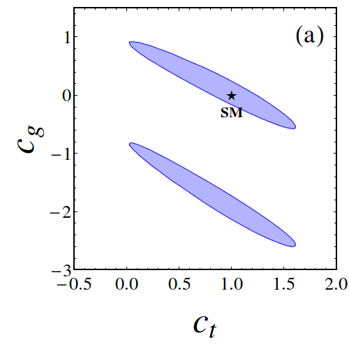
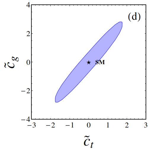
Figure 1: The current constraints at $95\%$ CL on $(c_{t},c_{g})$, $(c_{g},\tilde{c}_{g})$, $(c_{t},\tilde{c}_{t})$, $(\tilde{c}_{t},\tilde{c}_{g})$, $(c_{g},\tilde{c}_{t})$ and $(c_{t},\tilde{c}_{g})$. In each case, we consider only two couplings and set others to be the SM values.

In Fig. 1, we display the allowed regions of the effective couplings by the current single Higgs measurements at the LHC at $95\%$ confidence level (CL), which are shown in blue bands. Only two effective couplings vary in each plot while other couplings are set to be the SM values. Scenario $(c_{t},c_{g})$ shows two isolated bands, since the constraint from $\kappa_{g}^{2}$ is proportional to $|c_{t}F_{\triangle}+\frac{2}{3}c_{g}|^{2}$, which can be simplified as $|c_{g}+c_{t}|^{2}$ in the infinite $m_{t}$ limit. Therefore, there are two degenerate regions satisfying the constraints, $c_{g}+c_{t}\sim\pm 1$. Besides, the lower and upper limits of $c_{t}$ come from the constraint of $\kappa_{\gamma}^{2}$. So $c_{t}$ cannot be too small or large, otherwise $\Gamma(h\to\gamma\gamma)$ will be too large. The constraint on scenario $(c_{g},\tilde{c}_{g})$ comes only from $\kappa_{g}^{2}$, which is $|c_{g}+1|^{2}+|\tilde{c}_{g}|^{2}$ in the infinite $m_{t}$ limit. It’s obvious that in order to satisfy the single Higgs measurements, the allowed parameter space must be a ring. In scenario $(c_{t},\tilde{c}_{t})$, we have to consider both constraints on $\kappa_{g}^{2}$ and $\kappa_{\gamma}^{2}$. In the infinite $m_{t}$ limit, $\kappa_{g}^{2}$ is approximated to be $|c_{t}|^{2}+\frac{9}{4}|\tilde{c}_{t}^{2}|$. The allowed region from this constraint is an elliptical ring. The constraint on $\kappa_{\gamma}^{2}$ will further reject the $c_{t}\lesssim 0$ region. In scenario $(\tilde{c}_{t},\tilde{c}_{g})$, $\kappa_{g}^{2}\sim 1+|\tilde{c}_{g}-\frac{3}{2}\tilde{c}_{t}|^{2}$ in the infinite $m_{t}$ limit. The constraint on $\kappa_{g}^{2}$ will lead to $\tilde{c}_{g}\sim\frac{3}{2}\tilde{c}_{t}$, and $\kappa_{\gamma}^{2}$ will give lower and upper limits on $\tilde{c}_{t}$. The correlation in this scenario is different from scenario $(c_{t},c_{g})$ due to the relative minus sign between $F_{\triangle}$ and $F_{\triangle}^{(1)}$. Similar to scenario $(c_{g},\tilde{c}_{g})$ the allowed region is a ring in scenario $(c_{g},\tilde{c}_{t})$ as a fact of $\kappa_{g}^{2}\sim|c_{g}+1|^{2}+\frac{9}{4}|\tilde{c}_{t}|^{2}$. In principle, $\kappa_{\gamma}^{2}$ will further give a constraint on $\tilde{c}_{t}$. But it turns out that the constraint from $\kappa_{\gamma}^{2}$ is not so strong such that the region allowed by $\kappa_{g}^{2}$ satisfies the $\kappa_{\gamma}^{2}$ constraint. The situation of scenario $(c_{t},\tilde{c}_{g})$ is also similar to scenario $(c_{t},\tilde{c}_{t})$. In the infinite $m_{t}$ limit, we have $\kappa_{g}^{2}\sim|c_{t}|^{2}+|\tilde{c}_{g}|^{2}$.

On the other hand, the individual constraints on $c_{t}$, $\tilde{c}_{t}$, $c_{g}$ and $\tilde{c}_{g}$ at $95\%$ CL from the single Higgs measurements are

$$c_{t}\in[0.839,1.24],\ \tilde{c}_{t}\in[-0.345,0.186],\ c_{g}\in{[-2.134,-1.731]\cup[-0.161,0.242]},\ \tilde{c}_{g}\in[-0.279,0.517].$$ (10)

Apart from the LHC measurements, the CP-odd couplings are also constrained by the electric dipole moments of electron, neutron and mercury atom (Hg) Brod et al. (2013); Chien et al. (2015),

$$|\tilde{c}_{t}|<0.01,\ |\tilde{c}_{g}|<0.05.$$ (11)

III Double Higgs production

III.1 Amplitude

In this section, we will discuss the amplitude of double Higgs production via gluon fusion $gg\to hh$. The LO partonic amplitude of $g^{{a,\mu}}(p_{{1}})g^{{b,\nu}}(p_{{2}})\to h(p_{{3}})h(p_{{4}})$ with the effective Lagrangian in Eq. (I) is

$$\mathcal{M}_{hh} = \biggl{[}c_{t}^{2}\mathcal{M}_{\Box}^{SM}+\tilde{c}_{t}^{2}\mathcal{M}_{\Box}^{(1)}+c_{t}\tilde{c}_{t}\mathcal{M}_{\Box}^{(2)}+c_{t}c_{3h}\mathcal{M}_{\triangle}^{SM}+\tilde{c}_{t}c_{3h}\mathcal{M}_{\triangle}^{(1)}+c_{2t}\mathcal{M}_{\triangle}^{(2)}+\tilde{c}_{2t}\mathcal{M}_{\triangle}^{(3)}$$ (12)

$$~{}~{}+c_{g}c_{3h}\mathcal{M}_{g}^{(1)}+c_{g}\mathcal{M}_{g}^{(2)}+\tilde{c}_{g}c_{3h}\mathcal{M}_{g}^{(3)}+\tilde{c}_{g}\mathcal{M}_{g}^{(4)}\biggr{]}\epsilon^{{a}}_{\mu}(p_{{1}})\epsilon^{{b}}_{\nu}(p_{{2}})\delta^{ab},$$

where $a$ and $b$ in the superscript denote the color index of gluons,

$$\mathcal{M}_{\Box}^{SM}=-\frac{\alpha_{s}\hat{s}}{4\pi v^{2}}(F_{\Box}A^{\mu\nu}+G_{\Box}B^{\mu\nu}),$$

$$\mathcal{M}_{\Box}^{(1)}=-\frac{\alpha_{s}\hat{s}}{4\pi v^{2}}(F_{\Box}^{(1)}A^{\mu\nu}+G_{\Box}^{(1)}B^{\mu\nu}), \mathcal{M}_{\Box}^{(2)}=\frac{\alpha_{s}\hat{s}}{4\pi v^{2}}F_{\Box}^{(2)}C^{\mu\nu},$$

$$\mathcal{M}_{\triangle}^{SM}=-\frac{\alpha_{s}\hat{s}}{4\pi v^{2}}\frac{{m_{h}}^{2}}{\hat{s}-{m_{h}}^{2}}F_{\triangle}A^{\mu\nu}, \mathcal{M}_{\triangle}^{(1)}=\frac{\alpha_{s}\hat{s}}{4\pi v^{2}}\frac{3m_{H}^{2}}{\hat{s}-{m_{h}}f^{2}}F_{\triangle}^{(1)}C^{\mu\nu},$$

$$\mathcal{M}_{\triangle}^{(2)}=-\frac{\alpha_{s}\hat{s}}{4\pi v^{2}}F_{\triangle}A^{\mu\nu}, \mathcal{M}_{\triangle}^{(3)}=\frac{\alpha_{s}\hat{s}}{4\pi v^{2}}F_{\triangle}^{(1)}C^{\mu\nu},$$

$$\mathcal{M}_{g}^{(1)}=-\frac{\alpha_{s}\hat{s}}{4\pi v^{2}}\frac{3{m_{h}}^{2}}{\hat{s}-{m_{h}}^{2}}\frac{2}{3}A^{\mu\nu}, \mathcal{M}_{g}^{(2)}=-\frac{\alpha_{s}\hat{s}}{4\pi v^{2}}\frac{2}{3}A^{\mu\nu},$$

$$\mathcal{M}_{g}^{(3)}=\frac{\alpha_{s}\hat{s}}{4\pi v^{2}}\frac{3{m_{h}}^{2}}{\hat{s}-{m_{h}}^{2}}\frac{2}{3}C^{\mu\nu}, \mathcal{M}_{g}^{(4)}=\frac{\alpha_{s}\hat{s}}{4\pi v^{2}}\frac{2}{3}C^{\mu\nu}.$$ (13)

Here the Mandelstam variables of the partonic process are defined as

$$\hat{s}=(p_{{1}}+p_{{2}})^{2},\ \hat{t}=(p_{{1}}-p_{{3}})^{2},\ \hat{u}=(p_{{2}}-p_{{3}})^{2}.$$ (14)

The Lorentz structures $A^{\mu\nu}$ and $C^{\mu\nu}$ are defined in Eqs. (6) while $B^{\mu\nu}$ is Glover and van der Bij (1988); Plehn et al. (1996)

$$B^{\mu\nu} = g^{\mu\nu}+\frac{p_{{3}}^{2}p_{{1}}^{\nu}p_{{2}}^{\mu}}{p_{T}^{2}p_{{1}}\cdot p_{{2}}}-\frac{2p_{{2}}\cdot p_{{3}}p_{{1}}^{\nu}p_{{3}}^{\mu}}{p_{T}^{2}p_{{1}}\cdot p_{{2}}}-\frac{2p_{{1}}\cdot p_{{3}}p_{{2}}^{\mu}p_{{3}}^{\nu}}{p_{T}^{2}p_{{1}}\cdot p_{{2}}}+\frac{2p_{{3}}^{\mu}p_{{3}}^{\nu}}{p_{T}^{2}},$$ (15)

with $p_{T}^{2}=(\hat{u}\hat{t}-{m_{h}}^{4})/\hat{s}$. It can be easily verified that $A^{\mu\nu}A_{\mu\nu}=B^{\mu\nu}B_{\mu\nu}=C^{\mu\nu}C_{\mu\nu}=2$ and $A^{\mu\nu}B_{\mu\nu}=B^{\mu\nu}C_{\mu\nu}=A^{\mu\nu}C_{\mu\nu}=0$. Therefore we can expand the amplitude in terms of those tensor structures as follows

$$\mathcal{M}_{hh} = -\frac{\alpha_{s}\hat{s}\delta^{ab}}{4\pi v^{2}}\epsilon_{\mu}(p_{a})\epsilon_{\nu}(p_{b})\{[c_{t}^{2}F_{\Box}+\tilde{c}_{t}^{2}F_{\Box}^{(1)}+\frac{3{m_{h}}^{2}}{\hat{s}-{m_{h}}^{2}}c_{3h}(c_{t}F_{\triangle}+\frac{2}{3}c_{g})+\frac{2}{3}c_{g}+c_{2t}F_{\triangle}]A^{\mu\nu}$$ (16)

$$+ (c_{t}^{2}G_{\Box}+\tilde{c}_{t}^{2}G_{\Box}^{(1)})B^{\mu\nu}-[c_{t}\tilde{c}_{t}F_{\Box}^{(2)}+\frac{3{m_{h}}^{2}}{\hat{s}-{m_{h}}^{2}}c_{3h}(\tilde{c}_{t}F_{\triangle}^{(1)}+\frac{2}{3}\tilde{c}_{g})+\frac{2}{3}\tilde{c}_{g}+\tilde{c}_{2t}F_{\triangle}^{(1)}]C^{\mu\nu}\}.$$

The expressions of the form factors $F_{\Box}$, $G_{\Box}$, $F_{\Box}^{(1)}$, $G_{\Box}^{(1)}$, $F_{\Box}^{(2)}$, $F_{\triangle}$ and $F_{\triangle}^{(1)}$ can be found in Appendix A. In the large $m_{t}$ limit Plehn et al. (1996), we have

$$\begin{split}F_{\Box}&=-\frac{2}{3}+\mathcal{O}(\hat{s}/m_{t}^{2}),\qquad G_{\Box}=\mathcal{O}(\hat{s}/m_{t}^{2}),\qquad F_{\triangle}=\frac{2}{3}+\mathcal{O}(\hat{s}/m_{t}^{2}),\\ F_{\Box}^{(1)}&=\frac{2}{3}+\mathcal{O}(\hat{s}/m_{t}^{2}),\qquad F_{\Box}^{(2)}=2+\mathcal{O}(\hat{s}/m_{t}^{2}),\qquad G_{\Box}^{(1)}=\mathcal{O}(\hat{s}/m_{t}^{2}),\qquad F_{\triangle}^{(1)}=-1+\mathcal{O}(\hat{s}/m_{t}^{2}),\\ \end{split}$$ (17)

which can be obtained from the low energy theorem (LET) Shifman et al. (1979); Kniehl and Spira (1995).

Figure 2 shows the $\sqrt{\hat{s}}$-dependence of each form factor, where we have chosen two specific values of $\theta$ which is defined as the scattering angle of the initial gluon and final Higgs boson. Numerically, the $F$ form factors are always larger than the $G$ form factors around the threshold region $\sqrt{\hat{s}}\sim 400$ GeV, where the dominant cross section arises. Unlike the $G$ form factors, the $F$ form factors is insensitive to $\theta$. Thus the partonic cross section is dominated by the $s$-wave around the threshold region. To evaluate the $s$-wave and $d$-wave contributions at a large $\sqrt{\hat{s}}$, it is necessary to perform a partial wave analysis.

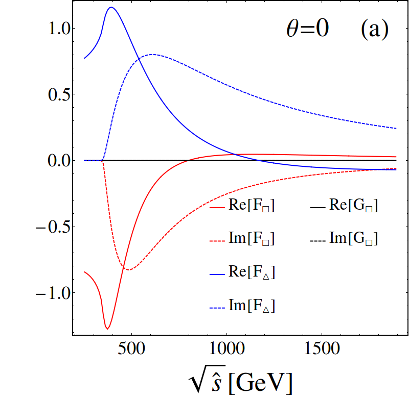
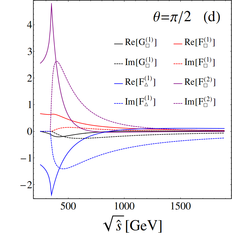
Figure 2: The form factors dependence on the partonic c.m. energy $\sqrt{\hat{s}}$, where we have chosen the scattering angle $\theta=0$ and $\pi/2$.

III.2 Partial wave analysis

The amplitude in the partial wave expansion is given by

$$\mathcal{M}_{hh}(\hat{s},\theta)=\sum_{\ell=0,2}(2\ell+1)\mathcal{M}_{\ell}(\hat{s})P_{\ell}(\cos\theta),$$ (18)

where $P_{\ell}(x)$ are the Legendre polynomials satisfy ing the orthogonal relation $\displaystyle{\int_{-1}^{1}dxP_{\ell}(x)P_{\ell^{\prime}}(x)=\frac{2}{(2\ell+1)}\delta_{\ell\ell^{\prime}}}$. The $s$-wave and $d$-wave components of the amplitude are proportional to $P_{0}(x)$ and $P_{2}(x)$ respectively, which are

$$\mathcal{M}_{0}(\hat{s}) = \frac{1}{2}\int_{-1}^{1}d\cos\theta\mathcal{M}_{hh}(\hat{s},\theta)P_{0}(\cos\theta),$$ (19)

$$\mathcal{M}_{2}(\hat{s}) = \frac{1}{2}\int_{-1}^{1}d\cos\theta\mathcal{M}_{hh}(\hat{s},\theta)P_{2}(\cos\theta).$$ (20)

Now the partonic level differential cross section with respect to $\cos\theta$ can be expanded into three terms

$$\frac{d\hat{\sigma}_{hh}(\hat{s})}{d\cos\theta}=\hat{\sigma}_{0}(\hat{s})+\hat{\sigma}_{2}(\hat{s})P_{2}(\cos\theta)^{2}+\hat{\sigma}_{\text{int}}{(\hat{s})}P_{2}(\cos\theta),$$ (21)

where the first and the second terms denote the $s$-wave and $d$-wave contributions, respectively. The third term, which arises from the interference of the $s$-wave and $d$-wave components of the amplitude, vanishes after integrating over $\cos\theta$. $\hat{\sigma}_{0}(\hat{s})$, $\hat{\sigma}_{2}(\hat{s})$ and $\hat{\sigma}_{\text{int}}{(\hat{s})}$ can be obtained numerically. The angular dependence of the form factors can be clearly revealed by choosing different combinations of ($c_{t},\tilde{c}_{t}$). In Fig. 3, we show the three terms in Eq. (21) with $\sqrt{\hat{s}}=400~{}\rm GeV,1000~{}\rm GeV$ for different $(c_{t},\tilde{c}_{t})$, where we fix other Higgs effective couplings to be the SM values and normalize the three terms to the total cross sections. Since the $s$-wave has no angular dependence, the distributions in Figs. 3(a) and (d) are flat. The $d$-wave and the interference contributions have nontrival angular dependences, which are reflected in Figs. 3(b, e) and (c, f), respectively. From the distributions, the $d$-wave and the interference contributions are comparable for $\sqrt{\hat{s}}=400~{}\rm GeV$ and $1000~{}\rm GeV$. This is because the imaginary (real) parts of the form factors at $\sqrt{\hat{s}}=400~{}(1000)~{}\rm GeV$ are small such that the interference contribution is suppressed. While increasing the $\sqrt{\hat{s}}$ from 400 GeV to 1000 GeV, the fractions of the $d$-wave and the interference contributions grow almost one order of magnitude. However, their contributions are still overwhelmed by the $s$-wave. So the $d$-wave and the interference contributions to $\cos\theta$ distributions at the hadron level, such as transverse momentum or rapidity distributions, are small. Figure 4 shows the $s$ and $d$-wave contributions to the total cross sections after integrating over $\cos\theta$. It is clear that the $d$-wave contributions are at most of $10\%$ of the total cross sections. As a result, the invariant mass distributions at the hadron level are dominated by the $s$-wave.

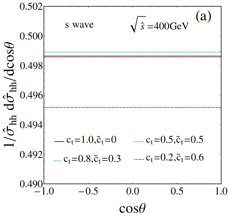
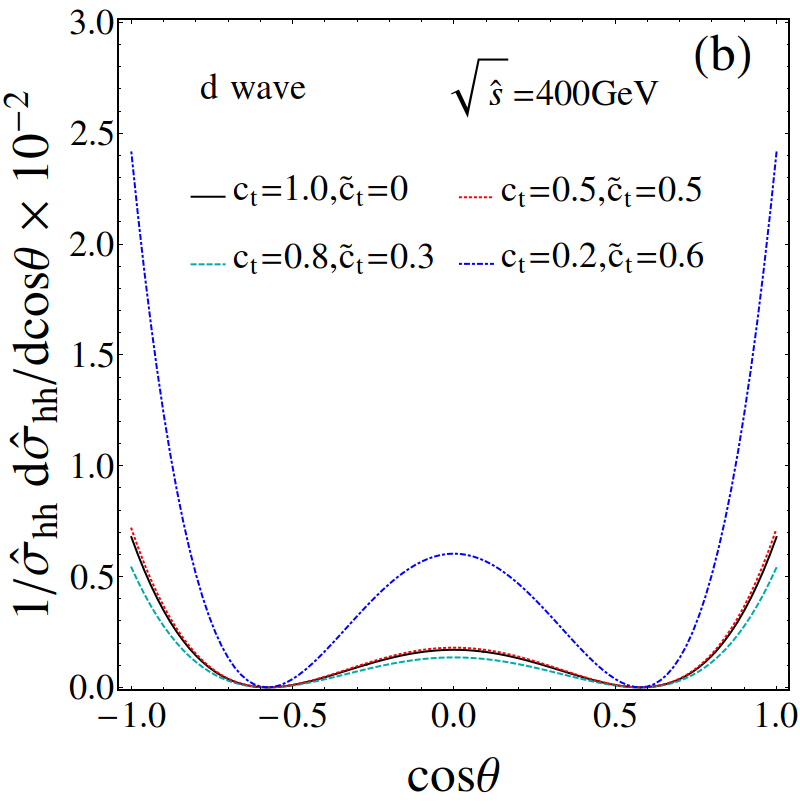
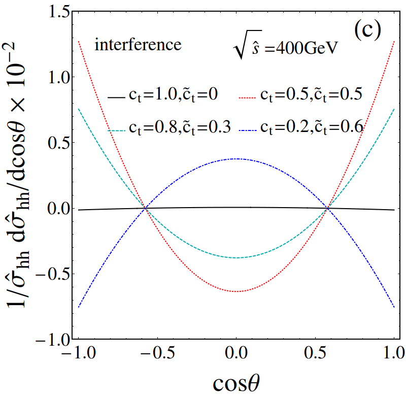
Figure 3: $\cos\theta$ distributions from the $s$-wave and $d$-wave contributions at $\sqrt{s}=400~{}\text{GeV},1000~{}\text{GeV}$. The black (solid), cyan (dashed), red (dot-dashed) and blue (dotted) lines correspond to $(c_{t},\tilde{c}_{t})=(1,0)$, $(0.8,0.3)$, $(0.5,0.5)$, $(0.2,0.6)$, respectively.

Figure 4: Fractions of the $s$-wave and $d$-wave contributions to the partonic cross section as a function of $\sqrt{\hat{s}}$ for different $c_{t}$ and $\tilde{c}_{t}$.

To be concrete, we show the $s$-wave and $d$-wave contributions to the total cross section at the hadron level,

$$\sigma_{0} =\int_{\tau_{0}}^{1}d\tau\int_{\tau}^{1}\frac{dx}{x}f_{g}(x;\mu_{F}^{2})f_{g}(\frac{\tau}{x};\mu_{F}^{2})\int_{-1}^{1}d\cos\theta\hat{\sigma}_{0}({\tau s})P_{0}(\cos\theta)^{2},$$ (22)

$$\sigma_{2} =\int_{\tau_{0}}^{1}d\tau\int_{\tau}^{1}\frac{dx}{x}f_{g}(x;\mu_{F}^{2})f_{g}(\frac{\tau}{x};\mu_{F}^{2})\int_{-1}^{1}d\cos\theta\hat{\sigma}_{2}({\tau s})P_{2}(\cos\theta)^{2},$$ (23)

where $\tau_{0}=4{m_{h}}^{2}/s$, $f_{g}$’s are the PDF functions of the initial gluons, and $\mu_{F}$ is the factorization scale. The hadronic cross sections can be expanded as follows,

$$\frac{\sigma_{0}}{\sigma^{SM}_{hh}} =a_{1}c_{t}^{4}+a_{2}c_{t}^{3}+a_{3}c_{t}^{2}\tilde{c}_{t}^{2}+a_{4}c_{t}^{2}+a_{5}c_{t}\tilde{c}_{t}^{2}+a_{6}\tilde{c}_{t}^{4}+a_{7}\tilde{c}_{t}^{2}{,}$$ (24)

$$\frac{\sigma_{2}}{\sigma^{SM}_{hh}} =b_{1}c_{t}^{4}+b_{2}c_{t}^{3}+b_{3}c_{t}^{2}\tilde{c}_{t}^{2}+b_{4}c_{t}^{2}+b_{5}c_{t}\tilde{c}_{t}^{2}+b_{6}\tilde{c}_{t}^{4}+b_{7}\tilde{c}_{t}^{2},$$ (25)

where $\sigma^{SM}_{hh}$ denotes the hadronic cross section of $gg\to hh$ in the SM, which has been calculated at the LO Eboli et al. (1987); Glover and van der Bij (1988); Plehn et al. (1996), NLO Dawson et al. (1998); Grigo et al. (2013); Frederix et al. (2014); Maltoni et al. (2014); Borowka et al. (2016a, b); Kerner (2016), NLL Ferrera and Pires (2016), NNLO de Florian and Mazzitelli (2013a, b); Grigo et al. (2014, 2015); Degrassi et al. (2016); de Florian et al. (2016); Hoff (2016) and NNLL Shao et al. (2013); de Florian and Mazzitelli (2015). The coefficients of the expansions are displayed in Table 1. Total cross sections at the 14 TeV LHC and the 100 TeV $pp$-collider are dominated by the $s$-wave component. Besides, the fractions of the $s$-wave contribution at the 100 TeV $pp$-collider are smaller than the fractions at the 14 TeV LHC, while the fractions of the $d$-wave contribution at the 100 TeV $pp$-collider are larger than the fractions at the 14 TeV LHC.

Table 1: The coefficients $a_{i}$ and $b_{i}$ at $\sqrt{s}=14~{}\rm TeV$ and 100 TeV.

$\sqrt{s}$	$a_{1}$	$a_{2}$	$a_{3}$	$a_{4}$	$a_{5}$	$a_{6}$	$a_{7}$
$14~{}\rm TeV$	2.069	-1.351	13.858	0.276	-6.219	0.706	0.861
$100~{}\rm TeV$	1.891	-1.108	11.280	0.208	-4.795	0.663	0.634
$\sqrt{s}$	$b_{1}$	$b_{2}$	$b_{3}$	$b_{4}$	$b_{5}$	$b_{6}$	$b_{7}$
$14~{}\rm TeV$	0.006	0	0.020	0	-0.136	0.013	0
$100~{}\rm TeV$	0.009	0	0.027	0	-0.137	0.017	0

From the above partial wave analysis, we draw a few conclusions, which do not rely on the Higgs effective couplings.

1. The $d$-wave contributions to the $\cos\theta$ distributions at the hadron level, such as transverse momentum or rapidity distributions, are always small;

2. The $d$-wave contributions to the invariant mass distributions at the hadron level are small;

3. The $d$-wave contributions to the total cross sections are small.

Therefore, it is justified that the double Higgs production is dominated by the $s$-wave.

IV Collider simulation

In Table 2 we collect references of the searches of double Higgs production at the 8 TeV and the 13 TeV LHC as well as the projected analyses at HL-LHC and 100 TeV $pp$-collider in the final states $b\bar{b}\gamma\gamma$, $b\bar{b}b\bar{b}$, $b\bar{b}\tau^{+}\tau^{-}$, $b\bar{b}W^{+}W^{-}$, $\gamma\gamma W^{+}W^{-}$ and $b\bar{b}VV(V=W,Z)$. Although $b\bar{b}b\bar{b}$ channel has the largest cross section, the QCD background is hard to control. On the other hand, the $b\bar{b}\gamma\gamma$ channel, despite of its small decay branching ratio, exhibits clear collider signature. Therefore, it has been studied extensively in the literature Baur et al. (2004); Contino et al. (2012); Baglio et al. (2013); Chen and Low (2014); Azatov et al. (2015); Cao et al. (2015). In this study, we focus our attention on the $b\bar{b}\gamma\gamma$ channel and use the cut efficiency function $\mathcal{A}(m_{hh})$ to mimic the detector effects in different NP scenarios. At the 14 TeV HL-LHC, we follow the analysis done by the ATLAS Collaboration ATLAS Collaboration (2015a) and adopt the cut efficiency function in Ref. Cao et al. (2015). At the 100 TeV $pp$-collider, we follow the projected analysis done by the 100 TeV group Contino et al. (2016). In the rest of this section, we will first derive cut efficiency function of $gg\to hh\to b\bar{b}\gamma\gamma$ at the 100 TeV $pp$-collider, then we will discuss the correlations and sensitivities of Higgs effective couplings.

Table 2: Searches of double Higgs production at the $8~{}\rm{TeV}$ and $13~{}\rm TeV$ by the ATLAS and CMS Collaborations, as well as the projected analysis at the $14~{}\rm{TeV}$ High-Luminosity LHC (HL-LHC) and the $100~{}\rm TeV$ $pp$-collider.

		$b\bar{b}\gamma\gamma$	$b\bar{b}b\bar{b}$	$b\bar{b}\tau^{+}\tau^{-}$	$\gamma\gamma W^{+}W^{-}$	$b\bar{b}VV$
$8~{}\rm{TeV}$	ATLAS	Aad et al. (2015a, b)	Aad et al. (2015c, b)	Aad et al. (2015b)	Aad et al. (2015b)	-
$8~{}\rm{TeV}$	CMS	CMS Collaboration (2014)	Khachatryan et al. (2015a)	CMS Collaboration (2016b)Khachatryan et al. (2016)	-	-
$13~{}\rm{TeV}$	ATLAS	The ATLAS Collaboration (2016)	Aaboud et al. (2016)	-	-	-
$13~{}\rm{TeV}$	CMS	CMS Collaboration (2016c)	CMS Collaboration (2016d)CMS Collaboration (2016e)	CMS Collaboration (2016f)CMS Collaboration (2016g)CMS Collaboration (2016h)CMS Collaboration (2016i)	-	CMS Collaboration (2016j)CMS Collaboration (2016k)
$14~{}\rm{TeV}$ HL-LHC	ATLAS	ATLAS Collaboration (2015a)	-	ATLAS Collaboration (2015b)	-	-
$14~{}\rm{TeV}$ HL-LHC	CMS	CMS Collaboration (2015b)	-	CMS Collaboration (2015b)	CMS Collaboration (2015b)	-
$100~{}\rm{TeV}$ $pp$-collider	Contino, et. al.	Contino et al. (2016)	Contino et al. (2016)	Contino et al. (2016)	Contino et al. (2016)	Contino et al. (2016)

IV.1 Cut efficiency function

The Born level differential cross section of double Higgs production can be written as

$$\frac{d^{2}\sigma}{dm_{hh}d\eta}=\frac{1}{2S}\int dx_{1}dx_{2}H\left(\hat{s},\hat{\eta},\mu_{r},\{\theta_{NP}\}\right)f_{g/p}\left(x_{1},\mu_{f}\right)f_{g/p}\left(x_{2},\mu_{f}\right)\delta\left(x_{1}x_{2}S-\hat{s}\right)\det\left[\frac{\partial\left(\hat{s},\hat{\eta}\right)}{\partial\left(m_{hh},\eta\right)}\right],$$ (26)

where $H$ is the hard scattering cross section depending on the center of mass energy (c.m.) square $\hat{s}$ and Higgs boson pseudo-rapidity $\hat{\eta}$ in the c.m. frame, $S$ is the collision energy of the hadron collider, $\mu_{f}$ is the factorization scale, $f_{i/j}$ is the parton distribution function (PDF) of parton $i$ from $j$, $m_{hh}$ is the invariant mass of Higgs boson pair in the lab frame, $\eta$ ($\hat{\eta}$) is the pseudo-rapidity of Higgs boson in the lab frame (c.m. frame), $\{\theta_{NP}\}$ are the parameters from the new physics model. We do not write the parameters ${m_{h}}^{2}$ and $m_{t}^{2}$ explicitly, the azimuthal angle has been integrated out.

We know that $\hat{s}=m_{hh}^{2}$ at the Born level. The Jacobian determinant is $2m_{hh}|\partial\hat{\eta}/\partial\eta|$, and

$$\frac{d^{2}\sigma}{dm_{hh}d\eta} = \frac{m_{hh}}{S}\int dx_{1}dx_{2}\left|\frac{\partial\hat{\eta}}{\partial\eta}\right|H\left(m_{hh},\hat{\eta}\left(m_{hh},\eta,\frac{x_{1}}{x_{2}}\right),\mu_{r}\right)f_{g/p}\left(x_{1},\mu_{f}\right)f_{g/p}\left(x_{2},\mu_{f}\right)\delta\left(x_{1}x_{2}S-m_{hh}^{2}\right)$$ (27)

$$= \int^{1}_{m_{hh}^{2}/S}\frac{m_{hh}dx_{1}}{x_{1}S^{2}}H\left(m_{hh},\hat{\eta}\left(m_{hh},\eta,\frac{x_{1}^{2}S}{m_{hh}^{2}}\right),\mu_{r}\right)f_{g/p}\left(x_{1},\mu_{f}\right)f_{g/p}\left(\frac{m_{hh}^{2}}{x_{1}S},\mu_{f}\right)\left|\frac{\partial\hat{\eta}}{\partial\eta}\right|.$$

The $\eta$ and $\hat{\eta}$ are related by

$$\eta=-\frac{1}{2}\log\left[\frac{\sqrt{\Delta^{2}+4x_{1}x_{2}\beta^{2}{\text{sech}}^{2}\hat{\eta}}-\Delta}{\sqrt{\Delta^{2}+4x_{1}x_{2}\beta^{2}{\text{sech}}^{2}\hat{\eta}}+\Delta}\right],$$ (28)

where

$$\beta\equiv \displaystyle\sqrt{1-\frac{4m_{h}^{2}}{m_{hh}^{2}}},\ \Delta\equiv \left(x_{1}-x_{2}\right)+\left(x_{1}+x_{2}\right)\beta\tanh\hat{\eta}.$$ (29)

Thus

$$\frac{\partial\hat{\eta}}{\partial\eta}=\frac{\sqrt{\Delta^{2}+4x_{1}x_{2}\beta^{2}{\text{sech}}^{2}\hat{\eta}}}{\left(x_{1}+x_{2}\right)\beta+\left(x_{1}-x_{2}\right)\tanh\hat{\eta}},$$ (30)

For gluon-fusion initial state, the main contribution comes from the small-$x$ region with $x_{1}\sim x_{2}$. In that limit, it is a good approximation that $\hat{\eta}=\eta$.

Owing to the scalar feature of Higgs boson, the kinematics of Higgs boson decay products is mainly controlled by the Higgs kinematics, e.g. $p_{T}$ and $\eta$ of the Higgs boson. Thus the cut efficiency depends on the $p_{\text{T}}$ and $\eta$ distributions of Higgs bosons. The transverse momentum of Higgs boson is

$$p_{\text{T}}=\frac{\sqrt{\hat{s}}}{2}\beta{\text{sech}}\hat{\eta}=\frac{m_{hh}}{2}\beta{\text{sech}}\left[\hat{\eta}\left(m_{hh},\eta_{1},\frac{x_{1}^{2}S}{m_{hh}^{2}}\right)\right].$$ (31)

Denote $\epsilon\left(p_{\text{T}},\eta_{1},\eta_{2}\right)$ to be the differential cut efficiency function. The pseudo-rapidity $\eta_{2}$ is determined by $\hat{\eta}$, $m_{hh}$ and $x_{1}$. Therefore, $\epsilon$ is a function of $m_{hh}$, $x_{1}$ and $\eta$ (which is just $\eta_{1}$).

The hard scattering function, $H$, is generically $\eta$-dependent. Fortunately, for the SM-like double Higgs production induced by the effective Lagrangian given in Eq. (I), higher partial wave components are highly suppressed. Therefore, we can treat $\{\theta_{NP}\}$ as $\hat{\eta}$-independent. Then the amplitude square will be $\hat{\eta}$-independent. Under such assumptions, the differential cross section can be factorized as following,

$$\frac{d^{2}\sigma}{dm_{hh}d\eta} = \frac{m_{hh}}{S^{2}}H\left(m_{hh},\mu_{r}\right)\int^{1}_{m_{hh}^{2}/S}\frac{dx_{1}}{x_{1}}f_{g/p}\left(x_{1},\mu_{f}\right)f_{g/p}\left(\frac{m_{hh}^{2}}{x_{1}S},\mu_{f}\right)\left|\frac{\partial\hat{\eta}}{\partial\eta}\right|_{m_{hh},\eta,x_{1}}.$$ (32)

Integrating the pseudo-rapidity out, we have

$$\frac{d\sigma}{dm_{hh}} = \frac{m_{hh}}{S^{2}}H\left(m_{hh},\mu_{r}\right)\int^{1}_{m_{hh}^{2}/S}\frac{dx_{1}}{x_{1}}f_{g/p}\left(\frac{m_{hh}^{2}}{x_{1}S},\mu_{f}\right)f_{g/p}\left(x_{1},\mu_{f}\right)\int d\eta\left|\frac{\partial\hat{\eta}}{\partial\eta}\right|_{m_{hh},\eta,x_{1}}$$ (33)

$$\equiv \frac{m_{hh}}{S^{2}}H\left(m_{hh},\mu_{r}\right)\Sigma\left(m_{hh},S,\mu_{f}\right).$$

We can also write down the differential cross section after kinematic cuts used by experimental groups,

$$\frac{d\sigma_{\text{after~{}cuts}}}{dm_{hh}} = \int d\tilde{m}_{hh}\frac{\tilde{m}_{hh}}{S^{2}}H\left(\tilde{m}_{hh},\mu_{r}\right)\int^{1}_{\tilde{m}_{hh}^{2}/S}\frac{dx_{1}}{x_{1}}f_{g/p}\left(\frac{\tilde{m}_{hh}^{2}}{x_{1}S},\mu_{f}\right)f_{g/p}\left(x_{1},\mu_{f}\right)$$ (34)

$$\times\int d\eta\left|\frac{\partial\hat{\eta}}{\partial\eta}\right|_{\tilde{m}_{hh},\eta,x_{1}}\epsilon\left(m_{hh},\tilde{m}_{hh},x_{1},\eta\right),$$

where $m_{hh}$ is the invariant mass of the Higgs-pair system measured in the experiment, $\tilde{m}_{hh}$ is the real invariant mass of the Higgs-pair system of the same event, which is introduced to describe the finite energy smearing effect. For an ideal detector, we have

$$\epsilon\left(m_{hh},\tilde{m}_{hh},x_{1},\eta\right)=\epsilon\left(m_{hh},x_{1},\eta\right)\delta\left(\tilde{m}_{hh}-m_{hh}\right),$$ (35)

which will be broken by finite energy smearing effect. Due to the cut effect, in general

$$\epsilon\left(m_{hh},\tilde{m}_{hh},x_{1},\eta\right)\neq\epsilon\left(\tilde{m}_{hh},m_{hh},x_{1},\eta\right).$$ (36)

To investigate the inclusive result, one can integrate $m_{hh}$ and have

$$\sigma_{\text{after~{}cuts}} = \int dm_{hh}d\tilde{m}_{hh}\frac{\tilde{m}_{hh}}{S^{2}}H\left(\tilde{m}_{hh},\mu_{r}\right)\int^{1}_{\tilde{m}_{hh}^{2}/S}\frac{dx_{1}}{x_{1}}f_{g/p}\left(\frac{\tilde{m}_{hh}^{2}}{x_{1}S},\mu_{f}\right)f_{g/p}\left(x_{1},\mu_{f}\right)$$ (37)

$$\times\int d\eta\left|\frac{\partial\hat{\eta}}{\partial\eta}\right|_{\tilde{m}_{hh},\eta,x_{1}}\epsilon\left(m_{hh},\tilde{m}_{hh},x_{1},\eta\right).$$

Define

$$\tilde{\Sigma}\left(\tilde{m}_{hh},S,\mu_{f}\right) \equiv \int dm_{hh}\int^{1}_{\tilde{m}_{hh}^{2}/S}\frac{dx_{1}}{x_{1}}f_{g/p}\left(\frac{\tilde{m}_{hh}^{2}}{x_{1}S},\mu_{f}\right)f_{g/p}\left(x_{1},\mu_{f}\right)$$ (38)

$$\times\int d\eta\left|\frac{\partial\hat{\eta}}{\partial\eta}\right|_{\tilde{m}_{hh},\eta,x_{1}}\epsilon\left(m_{hh},\tilde{m}_{hh},x_{1},\eta\right),$$

we obtain

$$\sigma_{\text{after~{}cuts}}=\int d\tilde{m}_{hh}\frac{\tilde{m}_{hh}}{S^{2}}H\left(\tilde{m}_{hh},\mu_{r}\right)\tilde{\Sigma}\left(\tilde{m}_{hh},S,\mu_{f}\right).$$ (39)

Then it is natural to define a differential cut efficiency as

$${\mathcal{A}}\left(m_{hh},S,\mu_{f}\right)=\frac{\tilde{\Sigma}\left(m_{hh},S,\mu_{f}\right)}{\Sigma\left(m_{hh},S,\mu_{f}\right)}.$$ (40)

Such a differential cut acceptance function only depends on the collision energy and the detail of the PDF. When the new physics contribution is dominated by the $s$-wave, one can calculate the total cross section after cuts by a convolution of the differential cross section of of $m_{hh}$ and the differential cut acceptance function ${\mathcal{A}}(m_{hh},S,\mu_{f})$. Hence we obtain the master formula for our study as following

$$\sigma_{\text{after~{}cuts}} = \int d\tilde{m}_{hh}\frac{\tilde{m}_{hh}}{S^{2}}H\left(\tilde{m}_{hh},\mu_{r}\right)\tilde{\Sigma}\left(\tilde{m}_{hh},S,\mu_{f}\right)$$ (41)

$$= \int\frac{m_{hh}dm_{hh}}{S^{2}}H\left(m_{hh},\mu_{r}\right)\tilde{\Sigma}\left(m_{hh},S,\mu_{f}\right)$$

$$= \int\frac{m_{hh}dm_{hh}}{S^{2}}H\left(m_{hh},\mu_{r}\right)\Sigma\left(m_{hh},S,\mu_{f}\right){\mathcal{A}}\left(m_{hh},S,\mu_{f}\right)$$

$$= \int dm_{hh}\frac{d\sigma}{dm_{hh}}{\mathcal{A}}\left(m_{hh},S,\mu_{f}\right).$$

Equation (40) also tells us how to calculate the integral kernel ${\mathcal{A}}$ practically. It can be calculated by generating $s$-wave events with fixed $m_{hh}$ and counting the fraction of the events which pass the cuts. It is worth emphasizing that without the integration of $m_{hh}$, the result is not exactly the differential distribution due to the finite invariant mass smearing effect. However, when the smearing effect is not too large, it is a good approximation to mimic the differential distribution after cut as following

$$\left(\frac{d\sigma}{dm_{hh}}\right)_{\text{after cuts}}=\frac{d\sigma}{dm_{hh}}{\mathcal{A}}\left(m_{hh},S,\mu_{f}\right).$$ (42)

As to be shown soon, this approximation works well for the Higgs boson pair production. Thus we will use this approximation to illustrate the differential cross section in our work.

At the 100 TeV $pp$-collider, we can also use this analytical function to include all the detector effects as we did for 14 TeV LHC in Cao et al. (2015). We follow the strategy in the 100 TeV report Contino et al. (2016). The main backgrounds consist of $b\bar{b}\gamma\gamma$, $b\bar{b}j\gamma$, $jj\gamma\gamma$, $b\bar{b}h(\gamma\gamma)$ and $t\bar{t}h(\gamma\gamma)$. The cuts used are

$$\gamma~{}\text{isolation}~{}R=0.4,\ \text{jets: anti-kt, parameter}~{}R=0.4,\ \Delta R_{bb}<3.5~{},~{}\Delta R_{\gamma\gamma}<3.5,$$

$$p_{T}^{b_{1}}>60~{}{\rm{GeV}},~{}p_{T}^{b_{2}}>35~{}{\rm{GeV}},~{}|\eta^{b}|<4.5,\ p_{T}^{\gamma_{1}}>60~{}{\rm GeV},~{}p_{T}^{\gamma_{2}}>35~{}{\rm GeV},~{}|\eta^{\gamma}|<4.5,$$

$$p_{T}(bb)>100~{}{\rm GeV},p_{T}(\gamma\gamma)>100~{}{\rm GeV},\ 100{~{}\text{GeV}}<m_{b\bar{b}}<150{~{}\text{GeV}},\ {120.5}{~{}\text{GeV}}<m_{\gamma\gamma}<{129.5}{~{}\text{GeV}},$$ (43)

where $b_{1}$ ($b_{2}$) and $\gamma_{1}$ ($\gamma_{2}$) represent the leading (subleading) ${b}$-jet and photon, respectively. The ${b}$-tagging probability and faking rates are

$$p_{b\to b}=0.75,~{}p_{c\to b}=0.1,~{}p_{j\to b}=0.01.$$ (44)

The light-jet-to-photon faking probability is parametrized via

$$p_{j\to\gamma}=\alpha\exp(-p_{T,j}/\beta)~{},\alpha=0.01~{},\beta=30~{}\rm{GeV}.$$ (45)

The photon identification efficiency is

$$\epsilon_{\gamma}(p_{T})=\begin{cases}95\%,&~{}\text{for}~{}|\eta|<1.5,\\ 90\%,&~{}\text{for}~{}1.4<|\eta|<4,\\ 80\%,&~{}\text{for}~{}4<|\eta|<6.\end{cases}$$ (46)

To get the cut efficiency function, we generate partonic level $pp\to hh\to b\bar{b}\gamma\gamma$ events with MadGraph5_aMC@NLO event generator Alwall et al. (2014) with CT14 PDF Dulat et al. (2015). As we are interested only in the $s$-wave component, the default SM with trilinear Higgs coupling is enough. The events are generated with fixed $m_{hh}$ for each 10 GeV interval. The detector effects are mimicked with Gaussian smearing effects with the parameters given in Contino et al. (2016).

Figure 5: The cut efficiency function at the 100 TeV $pp$-collider.

We show the cut efficiency function for the 100 TeV $pp$-collider in Fig. 5. The structures in the figure can be easily understood as follows. For the “peak” structure, the boost factor of the Higgs boson is $\gamma\simeq 5$ around the crossing point. The angular distance between the Higgs decay products, i.e. $\Delta R\equiv\sqrt{(\Delta\eta)^{2}+(\Delta\phi)^{2}}$ is approximated by $\Delta R\simeq 2/\gamma\simeq 0.4$. So crossing this point, the typical $\Delta R$ of the $b\bar{b}$ system and the $\gamma\gamma$ system will become smaller. The signal events are likely to fail the $\Delta R$ cuts to yield a smaller cut efficiency. We would like to estimate the result analytically with some approximations. Let us define the 4-momenta of the partons (photons) in the Higgs rest frame with the $z$-direction defined by the Higgs 3-momentum in the lab frame. Then the exact result of the $\Delta R$ is

$$\Delta R^{2} =\arccos^{2}\biggl{\{}\biggl{[}4r^{2}\beta_{T}^{2}+\left(1-z^{2}\right)\left(\beta_{T}^{2}-\cos^{2}\phi-\sin^{2}\phi\tanh^{2}\eta\right)-z^{2}~{}\text{sech}^{2}\eta$$

$$+2z\sin\phi\tanh\eta\times\sqrt{\left(1-z^{2}\right)\left(\beta_{T}^{2}+~{}\text{sech}^{2}\eta\right)}\biggr{]}$$

$$\times\biggl{[}\left(1-z^{2}\right)\cos^{2}\phi+\biggl{(}\sqrt{1+4r^{2}}\beta_{T}-\sqrt{1-z^{2}}\sin\phi\tanh\eta+z\sqrt{\beta_{T}^{2}+~{}\text{sech}^{2}\eta}\biggr{)}^{2}\biggr{]}^{-\frac{1}{2}}$$

$$\times\biggl{[}\left(1-z^{2}\right)\cos^{2}\phi+\biggl{(}\sqrt{1+4r^{2}}\beta_{T}+\sqrt{1-z^{2}}\sin\phi\tanh\eta-z\sqrt{\beta_{T}^{2}+~{}\text{sech}^{2}\eta}\biggr{)}^{2}\biggr{]}^{-\frac{1}{2}}\biggr{\}}$$

$$+\biggl{\{}~{}\text{arcsinh}\biggl{\{}\biggl{[}\sinh\eta\left(\sqrt{1+4r^{2}}\beta_{T}+z\sqrt{\beta^{2}_{T}+~{}\text{sech}^{2}\eta}\right)+\sin\phi~{}\text{sech}\eta\sqrt{1-z^{2}}\biggr{]}$$

$$\times\biggl{[}\left(1-z^{2}\right)\cos^{2}\phi+\biggl{(}\sqrt{1+4r^{2}}\beta_{T}-\sqrt{1-z^{2}}\sin\phi\tanh\eta+z\sqrt{\beta_{T}^{2}+~{}\text{sech}^{2}\eta}\biggr{)}^{2}\biggr{]}^{-\frac{1}{2}}\biggr{\}}$$

$$+~{}\text{arcsinh}\biggl{\{}\biggl{[}\sinh\eta\left(-\sqrt{1+4r^{2}}\beta_{T}+z\sqrt{\beta^{2}_{T}+~{}\text{sech}^{2}\eta}\right)+\sin\phi~{}\text{sech}\eta\sqrt{1-z^{2}}\biggr{]}$$

$$\times\biggl{[}\left(1-z^{2}\right)\cos^{2}\phi+\biggl{(}\sqrt{1+4r^{2}}\beta_{T}+\sqrt{1-z^{2}}\sin\phi\tanh\eta-z\sqrt{\beta_{T}^{2}+~{}\text{sech}^{2}\eta}\biggr{)}^{2}\biggr{]}^{-\frac{1}{2}}\biggr{\}}\biggl{\}}^{2},$$ (47)

where $\beta_{T}\equiv p_{\text{T}}/m_{h}$ is the ratio between the transverse momentum and the mass of the Higgs boson in the lab frame, $r=m/m_{h}$ is the mass ratio between the final state particle and the Higgs boson, which is 0 for photon and $m_{b}/m_{h}$ for bottom quark, $\eta$ is the pseudo-rapidity of the Higgs boson in the lab frame, $z\equiv\cos\theta$ is the cosine value of the polar angle of one parton in the Higgs rest frame, $\phi$ is the azimuthal angle of one parton in the Higgs rest frame. In the highly boost region, $\beta_{T}\gg 1$, and

$$\Delta R=\arccos\left[1-\frac{2}{1+\left(1-z^{2}\right)\beta_{T}^{2}}\right]$$ (48)

is a good approximation for the massless final state particle. To pass the $\Delta R$ cuts, we need to solve this equation. The solutions are

$$z_{\pm}=\pm\sqrt{\frac{1-\beta_{T}^{-2}-\left(1+\beta_{T}^{-2}\right)\cos\Delta R}{1-\cos\Delta R}}.$$ (49)

The region allowed by the cut is $[-1,z_{-}]\cup[z_{+},1]$. This is a hint that we can fit the high invariant mass tail with the function

$$\mathcal{A}\left(m_{hh}\right)=c_{1}\left[1-\sqrt{\frac{m_{hh}^{2}\left(1-\cos\Delta R\right)-8\left(m_{h}-\delta m_{h}\right)^{2}}{\left(1-\cos\Delta R\right)\left(m_{hh}^{2}-4\left(m_{h}-\delta m_{h}\right)^{2}\right)}}\right]^{\gamma_{c}},$$ (50)

where $\Delta R=0.4$ is the angular distance cut, the parameter $\gamma_{c}$ and $\delta m$ reflect the energy resolution effect and the invariant mass cut effect, $c$ is a normalization constant.

For massive final state particle, we have

$$\Delta R=\arccos\left[\frac{\left(1-z^{2}+r^{2}\right)\beta_{T}^{2}-1}{\sqrt{\left[\left(1-z^{2}+r^{2}\right)\beta_{T}^{2}-1\right]^{2}+4\left(1-z^{2}\right)\left(1+4r^{2}\right)\beta_{T}^{2}}}\right].$$ (51)

The moving direction of a massive particle can be flipped by a Lorentz boost. For a very large $\beta_{T}>1/r$, $z\to\pm 1$, we have $\Delta R=0$. In this case, the region allowed by the cut is $[z_{-2},z_{-1}]\cup[z_{+1},z_{+2}]$ and could be $\varnothing$. However, because $m_{b}\ll m_{h}$, this will be only a tiny correction at very high $m_{hh}$ region ($p_{\text{T,cut}}^{h}>3.3$ TeV) and could be neglected.

The behavior of the cut efficiency function in the low invariant mass region can be understood as follows. The $p_{\text{T}}$ cuts on the Higgs bosons require the Higgs bosons have a large $p_{\text{T}}$, which means that the energy of the Higgs bosons must be larger than $\sqrt{m_{H}^{2}+p_{\text{T,cut}}^{2}}\simeq 160$ GeV. This is the reason why the events with $m_{hh}<320$ GeV have a very tiny (close to 0) cut acceptance. It is easy to know that the integration region of the polar angle in the c.m. frame is

$$\left[-\sqrt{1-\frac{4(p_{{\text{T,cut}}}^{h})^{2}}{m_{hh}^{2}-4m_{h}^{2}}},\sqrt{1-\frac{4(p_{{\text{T,cut}}}^{h})^{2}}{m_{hh}^{2}-4m_{h}^{2}}}\right].$$ (52)

This is a hint that we could fit the low invariant mass region with

$$\mathcal{A}\left(m_{hh}\right)=a_{1}\left[1-\frac{4(p_{{\text{T,cut}}}^{h})^{2}}{m_{hh}^{2}-4\left(m_{h}-\delta m_{2}\right)^{2}}\right]^{\beta_{a}}\left(\frac{2m_{h}}{m_{hh}}\right)^{\beta_{b}}\left[1+a_{2}\left(\frac{2m_{h}}{m_{hh}}\right)\log\left(\frac{2m_{h}}{m_{hh}}\right)\right],$$ (53)

where $p_{{\text{T,cut}}}^{h}=100$ GeV.

Finally, we obtain the analytic function $\mathcal{A}({m}_{hh},s,\mu_{F})$ at the 100 TeV $pp$-collider in the following form

$$\mathcal{A}\left({m}_{hh}\right)=\begin{cases}c_{1}\left[1-\sqrt{\dfrac{{m}_{hh}^{2}\left(1-\cos\Delta R_{0}\right)-8\left({m_{h}}-\delta m_{1}\right)^{2}}{\left(1-\cos\Delta R_{0}\right)\left({m}_{hh}^{2}-4\left({m_{h}}-\delta m_{1}\right)^{2}\right)}}\right]^{\gamma_{c}},&{m}_{hh}>M^{(t)}_{hh},\\ c_{2}\left[1-\displaystyle\frac{4(p_{{\text{T,cut}}}^{h})^{2}}{{m}_{hh}^{2}-4\left({m_{h}}-\delta m_{2}\right)^{2}}\right]^{\beta_{a}}\left(\dfrac{{2m_{h}}}{{m}_{hh}}\right)^{\beta_{b}}\left[1+\beta_{c}\left(\dfrac{{2m_{h}}}{{m}_{hh}}\right)\log\left(\dfrac{{2m_{h}}}{{m}_{hh}}\right)\right],&319.9{~{}\text{GeV}}<{m}_{hh}<M^{(t)}_{hh},\\ 0,&{m}_{hh}<319.9{~{}\text{GeV}}.\end{cases}$$ (54)

where the fitting parameters $\delta m_{1}=\delta m_{2}=0.15~{}\rm GeV$, $\Delta R_{0}=0.4$, $c_{1}={40.30}$, $\gamma_{c}={0.938}$, $c_{2}=8.269$, $\beta_{a}=1.241$, $\beta_{b}=-0.565$, $\beta_{c}=-2.057$, and $M_{hh}^{(t)}=1277.5$GeV, in the low detector performance scenario.

For completeness, we also show the cut efficiency function at the HL-LHC below. The selection cuts used by the ATLAS Collaboration ATLAS Collaboration (2015a) are

$$p_{T}^{b_{1}}>40~{}{\rm{GeV}},~{}p_{T}^{b_{2}}>25~{}{\rm{GeV}},~{}|\eta^{b}|<2.5,$$

$$p_{T}^{\gamma}>30~{}{\rm GeV},~{}|\eta^{\gamma}|<1.37~{}{\rm or}~{}1.52<|\eta^{\gamma}|<2.37,$$

$$\Delta R_{0}<\Delta R_{bb,\gamma\gamma}<2.0~{},~{}\Delta R_{b\gamma}>\Delta R_{0},~{}~{}\Delta R_{0}=0.4~{},$$

$$100{~{}\text{GeV}}<m_{bb}<150{~{}\text{GeV}},~{}p_{T}^{bb}>110{~{}\text{GeV}},$$

$$123{~{}\text{GeV}}<m_{\gamma\gamma}<128{~{}\text{GeV}},~{}p_{T}^{\gamma\gamma}>110{~{}\text{GeV}},$$ (55)

To mimic the detector effects, the final state parton momenta are smeared by a Gaussion distribution. The $b$-tagging efficiency is ATLAS Collaboration (2013a); Cao et al. (2015)

$$\epsilon_{b}\left(p_{T},\eta\right) = 0.135\tanh\left(\frac{p_{T}+50}{75}\right)\tanh\left(\frac{450}{p_{T}+80}\right)\times\big{[}3+e^{-\left(|\eta|-\sqrt{p_{T}/1000}\right)^{2}/1.6}\big{]}e^{-|\eta|^{3}p_{T}/1000}.$$ (56)

and the photon energy resolution and identification efficiency are ATLAS Collaboration (2013b)

$$\sigma\left({\text{GeV}}\right) = 0.3\oplus 0.10\times\sqrt{E({\text{GeV}})}\oplus 0.010\times E({\text{GeV}}),~{}~{}{\text{for}}~{}~{}|\eta|<1.37,$$

$$\sigma\left({\text{GeV}}\right) = 0.3\oplus 0.15\times\sqrt{E({\text{GeV}})}\oplus 0.015\times E({\text{GeV}}),~{}~{}{\text{for}}~{}~{}1.52<|\eta|<2.37,$$ (57)

and

$$\epsilon_{\gamma}\left(p_{T}\right)=0.76-1.98\exp\left(-\frac{p_{T}}{16.1{\text{GeV}}}\right),$$ (58)

respectively.

After fitting the Monte Carlos simulation results with all the detector effects, we obtain the following cut efficiency function with $p_{\rm T,cut}^{h}=110~{}{\rm GeV}$, which is slightly different from the function of the 100 TeV machine,

$$\mathcal{A}\left(M_{hh}\right)=\begin{cases}c_{1}\left[1-\sqrt{\dfrac{M_{hh}^{2}\left(1-\cos\Delta R_{0}\right)-8\left(m_{H}-\delta m_{1}\right)^{2}}{\left(1-\cos\Delta R_{0}\right)\left(M_{hh}^{2}-4\left(m_{H}-\delta m_{1}\right)^{2}\right)}}\right]^{\gamma_{c}},&M_{hh}>M^{(t)}_{hh},\\ c_{2}\left[1-\displaystyle\frac{4(p_{\rm T,cut}^{h})^{2}}{M_{hh}^{2}-4\left(m_{H}-\delta m_{2}\right)^{2}}\right]^{\beta_{a}}\left(\dfrac{M_{hh}}{\sqrt{s}}\right)^{\beta_{b}}\left[1+\beta_{c}\left(\dfrac{M_{hh}}{\sqrt{s}}\right)\log\left(\dfrac{2M_{hh}}{\sqrt{s}}\right)\right],&329.3{~{}\text{GeV}}<M_{hh}<M^{(t)}_{hh},\\ 0,&M_{hh}<329.3{~{}\text{GeV}}.\end{cases}$$ (59)

The fitting parameters are $c_{1}=1.1378$, $c_{2}=11.02$, $\delta m_{1}=50~{}\rm GeV$, $\gamma_{c}=1.675$, $\delta m_{2}=2.5~{}\rm GeV$, $\beta_{a}=1.13$, $\beta_{b}=1.48$, $\beta_{c}=4.88$, $\Delta R_{0}=0.4$ and $M_{hh}^{t}=1260~{}{\rm GeV}$ Cao et al. (2015).

IV.2 The $m_{hh}$ distribution

Once knowing the cut efficiency function $\mathcal{A}(m_{hh})$, one can calculate numbers of events of Higgs boson pair production after a series of kinematic cuts listed in Eq. (43) or Eq. (55) using the master formula shown in Eq. (41). That requires knowledge of the inclusive $m_{hh}$ distribution. Below we examine the impact of various effective couplings on the $m_{hh}$ distribution before and after imposing experimental cuts.

Figure 6 displays the $m_{hh}$ distributions in the double Higgs production with CP-violating $htt$ and $h(h)gg$ couplings before and after the selection cuts at the 14 TeV LHC and at a future 100 TeV $pp$-collider, respectively. We derive the $m_{hh}$ distribution after cuts by convoluting the inclusive distribution with the cut efficiency function as stated in Eq. (42). Two combinations of Higgs effective couplings, $(c_{t},\tilde{c}_{t})$ and $(c_{g},\tilde{c}_{g})$, are considered. We fix all the other effective couplings as the SM values while varying the two effective couplings in each combination. We choose a few benchmark couplings listed as follows:

$$(c_{t},\tilde{c}_{t}) = (1,~{}0),~{}~{}(~{}0.8,~{}0.3),~{}~{}(~{}~{}0.5,~{}0.5),~{}~{}~{}~{}(~{}0.2,0.6),$$

$$(c_{g},\tilde{c}_{g}) = (0,~{}0),~{}~{}(-2.0,~{}0),~{}~{}~{}(-1,~{}1),~{}~{}~{}~{}~{}~{}~{}~{}(-0.3,0.6),$$ (60)

which are well consistent with the measurements of single Higgs production at the LHC Run-I.

For the case of $(c_{t},\tilde{c}_{t})$, the invariant mass distribution of Higgs boson pairs peaks around 400 GeV in the SM, i.e. $(c_{t},\tilde{c}_{t})=(1,0)$; see the black-solid curves in Figs. 6(a) and (b). Other values of $c_{t}$ and $\tilde{c}_{t}$ shift the peak to small $m_{hh}$ regions both at the 14 TeV and at the 100 TeV. It can be understood as follows. In the SM, a large cancellation between $F_{\Box}$ and $F_{\triangle}\times 3m_{h}^{2}/(\hat{s}-m_{h}^{2})$ occurs near the threshold $m_{hh}\sim 2m_{h}\approx 250~{}{\rm GeV}$ Shifman et al. (1979); Kniehl and Spira (1995). However, the cancellation is spoiled when the $c_{t}$ coupling deviates sizably from the SM value $c_{t}=1$. That shifts the peak position. In addition, the contribution from $\tilde{c}_{t}(c_{t}F_{\Box}^{(2)}+F_{\triangle}^{(1)}\times 3m_{h}^{2}/(\hat{s}-m_{h}^{2}))$ increases dramatically with $\tilde{c}_{t}$. Therefore, a large $\tilde{c}_{t}$, e.g. $(c_{t},\tilde{c}_{t})=(0.2,0.6)$, distorts the smooth $m_{hh}$ distribution; see the blue curves in Figs 6(a) and (b). We notice that the $m_{hh}$ distributions do not change much when increasing the collider energy from 14 TeV to 100 TeV. The $m_{hh}$ distributions in the small $m_{hh}$ region is sensitive to $c_{t}$ and $\tilde{c}_{t}$ before imposing any cuts. Different choices of $c_{t}$ and $\tilde{c}_{t}$ couplings yield distinct distributions. Unfortunately, the differences in low $m_{hh}$ region are washed out once imposing a hard $p_{T}$ cut on the Higgs boson in order to disentangle the signal out of huge SM background at the 14 TeV LHC and the 100 TeV $pp$-collider. Figures 6(e) and (f) show the $m_{hh}$ distributions after the selection cuts given in Eq. (55). After cuts all the curves are quite similar. If NP models only modify the $c_{t}$ and $\tilde{c}_{t}$ coupling, then it is difficult to discriminate the NP models through the $m_{hh}$ distributions.

We also show the $m_{hh}$ distributions for various combinations of $(c_{g},\tilde{c}_{g})$ in Fig. 6. The $c_{g}$ and $\tilde{c}_{g}$ couplings introduce a momentum dependence to the double Higgs production, and they are expected to play an important role in large $m_{hh}$ region. In the small $m_{hh}$ region, the invariant mass distributions are distorted at the 14 TeV and 100 TeV colliders, owing to the weaker cancellation when $c_{g}<0$. In the high $m_{hh}$ regions, say $m_{hh}\gtrsim 400~{}\text{GeV}$, the distributions are distinctly different, especially at the 100 TeV collider. See Figs. 6(c) and (d). It is because, unlike the $F$ form factors, the contributions from $h(h)gg$ interaction, which are proportional to $c_{g}$ and $\tilde{c}_{g}$, do not decrease in the large $m_{hh}$ region. More importantly, the differences of the $m_{hh}$ distributions remain even after imposing the selection cuts; see Figs. 6(g) and (h). As a consequence, it is possible to discriminate different NP models that modify $c_{g}$ and $\tilde{c}_{g}$ through the $m_{hh}$ distributions.

Next, we will discuss the correlation and sensitivity of the Higgs effective couplings in the scattering of $gg\to hh\to b\bar{b}\gamma\gamma$ at the 14 TeV LHC and the 100 TeV $pp$-collider.

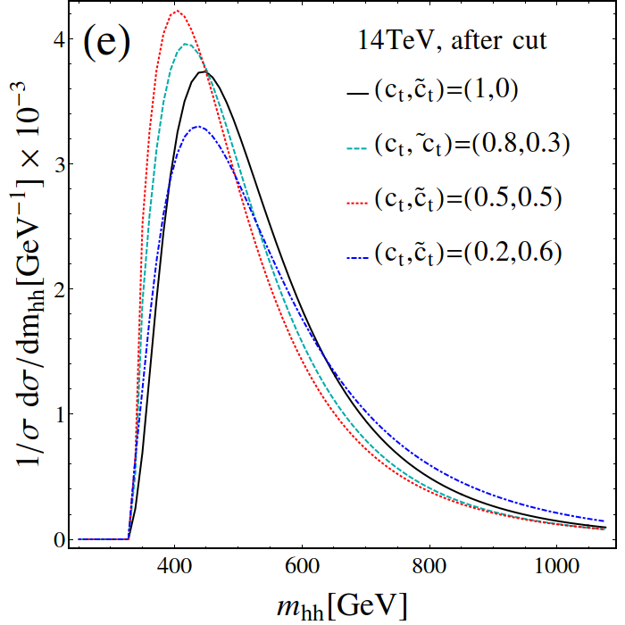
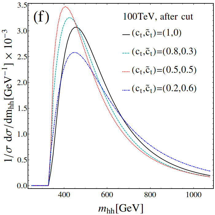
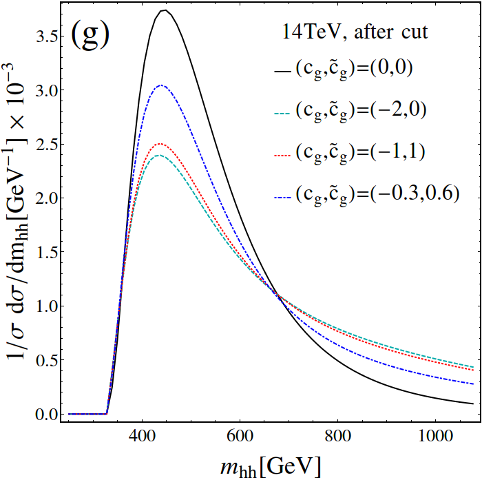
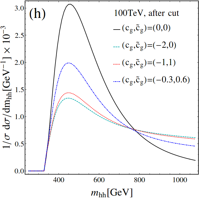
Figure 6: $m_{hh}$ distributions in the double Higgs production with CP-violating $htt$ and $h(h)gg$ couplings at the $14~{}\rm TeV$ LHC and the $100~{}\rm TeV$ $pp$-collider before (top row) and after the kinematic cuts (bottom row). The black (solid), green (dashed), red (dotdashed) and blue (dotted) lines in the upper panel correspond to $(c_{t},\tilde{c}_{t})=(1,0)$, $(0.8,0.3)$, $(0.5,0.5)$, $(0.2,0.6)$, respectively. While the black (solid), green blue (dashed), red (dotdashed) and blue (dotted) lines in the lower panel correspond to $(c_{g},\tilde{c}_{g})=(0,0),(-2,0),(-1,1),(-0.3,0.6)$, respectively.

IV.3 Signal strength and Higgs effective couplings

With the help of the cut efficiency function, we can easily obtain the total cross section of any NP described by the Higgs effective couplings after the selection cuts. Making use of the narrow width of the Higgs boson, the signal strength of the signal process, $pp\to hh\to b\bar{b}\gamma\gamma$, can be factorized as follows

$${\frac{\sigma(pp\to hh\to b\bar{b}\gamma\gamma)}{\sigma_{SM}(pp\to hh\to b\bar{b}\gamma\gamma)}} =\frac{\sigma_{hh}(pp\to hh)}{\sigma_{hh}^{SM}(pp\to hh)}\times\frac{\text{Br}(h\to b\bar{b})}{\text{Br}(h\to b\bar{b})_{SM}}\times\frac{\text{Br}(h\to\gamma\gamma)}{\text{Br}(h\to\gamma\gamma)_{SM}}\equiv\mu_{hh}\times\mu_{b\bar{b}}\times\mu_{\gamma\gamma},$$ (61)

where $\mu_{hh,b\bar{b},\gamma\gamma}$ denote the signal strength of the cross section of double Higgs production, of the branching ratio of $h\to b\bar{b}$ decay, of the branching ratio of $h\to\gamma\gamma$ decay, defined as follows:

$$\mu_{hh}\equiv\frac{\sigma_{hh}}{\sigma_{hh}^{SM}},\quad\mu_{b\bar{b}}\equiv\frac{\text{Br}(h\to b\bar{b})}{\text{Br}(h\to b\bar{b})_{SM}},\quad\mu_{\gamma\gamma}\equiv\frac{\text{Br}(h\to\gamma\gamma)}{\text{Br}(h\to\gamma\gamma)_{SM}}.$$ (62)

The dependence of $\mu_{hh}$ on the effective couplings is

$$\mu_{hh} =A_{1}c_{3h}^{2}c_{g}^{2}+A_{2}c_{3h}^{2}c_{g}c_{t}+A_{3}c_{3h}^{2}c_{t}^{2}+A_{4}c_{3h}c_{g}^{2}+A_{5}c_{3h}c_{g}c_{t}^{2}+A_{6}c_{3h}c_{g}c_{t}+A_{7}c_{3h}c_{g}\tilde{c}_{t}^{2}$$

$$+A_{8}c_{3h}c_{t}^{3}+A_{9}c_{3h}c_{t}\tilde{c}_{t}^{2}+A_{10}c_{g}^{2}+A_{11}c_{g}c_{t}^{2}+A_{12}c_{g}\tilde{c}_{t}^{2}+A_{13}c_{t}^{4}+A_{14}c_{t}^{2}\tilde{c}_{t}^{2}+A_{15}\tilde{c}_{t}^{4}$$

$$+A_{16}c_{3h}^{2}\tilde{c}_{g}^{2}+A_{17}c_{3h}^{2}\tilde{c}_{g}\tilde{c}_{t}+A_{18}c_{3h}^{2}\tilde{c}_{t}^{2}+A_{19}c_{3h}\tilde{c}_{g}^{2}+A_{20}c_{3h}\tilde{c}_{g}c_{t}\tilde{c}_{t}+A_{21}c_{3h}\tilde{c}_{g}\tilde{c}_{t}$$

$$+A_{22}\tilde{c}_{g}^{2}+A_{23}\tilde{c}_{g}c_{t}\tilde{c}_{t}+A_{24}c_{2t}^{2}+A_{25}c_{2t}c_{3h}c_{g}+A_{26}c_{2t}c_{3h}c_{t}+A_{27}c_{2t}c_{g}+A_{28}c_{2t}c_{t}^{2}$$

$$+A_{29}c_{2t}\tilde{c}_{t}^{2}+A_{30}c_{t}\tilde{c}_{t}\tilde{c}_{2t}+A_{31}c_{3h}\tilde{c}_{t}\tilde{c}_{2t}+A_{32}c_{3h}\tilde{c}_{g}\tilde{c}_{2t}+A_{33}\tilde{c}_{2t}^{2}+A_{34}\tilde{c}_{g}\tilde{c}_{2t}.$$ (63)

The product of $\mu_{b\bar{b}}$ and $\mu_{\gamma\gamma}$ is

$$\mu_{b\bar{b}}\times\mu_{\gamma\gamma} =\frac{\Gamma(h\to\gamma\gamma)}{\Gamma(h\to\gamma\gamma)_{SM}}\left(\frac{\Gamma_{tot}^{SM}}{\Gamma_{tot}}\right)^{2}=\frac{\kappa_{\gamma}^{2}}{\left[1+(\kappa_{g}^{2}-1)\text{BR}_{g}^{SM}+(\kappa_{\gamma}^{2}-1)\text{BR}_{\gamma}^{SM}\right]^{2}}$$ (64)

where we assume the Yukawa coupling of bottom quarks is not altered by NP effects. The $\kappa_{g}$ and $\kappa_{\gamma}$ couplings are defined in Eqs. (7) and (8). The SM branching ratios are $\text{BR}_{g}^{SM}\equiv\text{BR}(h\to gg)_{SM}=8.187\%$ and $\text{BR}_{\gamma}^{SM}\equiv\text{BR}(h\to\gamma\gamma)_{SM}=0.227\%$ Patrignani et al. (2016).

The values of the coefficients $A$’s are listed in Table 3 at the 14 TeV LHC and the 100 TeV $pp$-collider, before imposing any cuts (top panel) and after the series of cuts defined in Eq. 43 (bottom panel). The values of those coefficients at the 14 TeV LHC without any cut agree exactly with those values given in Ref. Azatov et al. (2015). We notice that the $A_{10,12,22,24}$ coefficients are larger at the 100 TeV $pp$-collider than at the 14 TeV LHC. Those coefficients correspond to the couplings of $c_{g}^{2}$, $c_{g}\tilde{c}_{t}^{2}$, $\tilde{c}_{g}^{2}$ and $c_{2t}^{2}$, which modify the $h(h)gg$ and $hhtt$ interactions and contribute significantly to the double Higgs production at the large $m_{hh}$ region.

Table 3: The cross sections of $gg\to hh\to b\bar{b}\gamma\gamma$ in terms of the Higgs effective couplings at the 14 TeV LHC and 100 TeV $pp$-collider before (top panel) and after (bottom panel) the selection cuts.

$\sqrt{s}$	$A_{1}$	$A_{2}$	$A_{3}$	$A_{4}$	$A_{5}$	$A_{6}$	$A_{7}$	$A_{8}$	$A_{9}$	$A_{10}$	$A_{11}$	$A_{12}$
$14~{}\rm TeV$	0.138	0.370	0.276	0.640	-0.766	0.821	0.535	-1.35	-6.22	1.37	-1.82	1.58
$100~{}\rm TeV$	0.101	0.267	0.208	0.592	-0.569	0.658	0.425	-1.11	-4.79	3.32	-1.30	1.67
$\sqrt{s}$	$A_{13}$	$A_{14}$	$A_{15}$	$A_{16}$	$A_{17}$	$A_{18}$	$A_{19}$	$A_{20}$	$A_{21}$	$A_{22}$	$A_{23}$	$A_{24}$
$14~{}\rm TeV$	2.07	13.9	0.719	0.138	-0.611	0.861	0.640	2.13	-1.24	1.37	4.64	2.55
$100~{}\rm TeV$	1.90	11.3	0.680	0.101	-0.428	0.634	0.592	1.53	-0.928	3.32	3.51	2.90
$\sqrt{s}$	$A_{25}$	$A_{26}$	$A_{27}$	$A_{28}$	$A_{29}$	$A_{30}$	$A_{31}$	$A_{32}$	$A_{33}$	$A_{34}$
$14~{}\rm TeV$	0.821	1.39	2.44	-4.24	2.30	-18.8	4.04	-1.24	6.19	-3.02
$100~{}\rm TeV$	0.658	1.21	2.06	-4.13	2.16	-16.3	3.28	-0.928	6.10	-2.08
$\sqrt{s}$	$A_{1}$	$A_{2}$	$A_{3}$	$A_{4}$	$A_{5}$	$A_{6}$	$A_{7}$	$A_{8}$	$A_{9}$	$A_{10}$	$A_{11}$	$A_{12}$
$14~{}\rm TeV$	0.0369	0.0975	0.0993	0.406	-0.264	0.410	0.239	-0.739	-2.46	1.80	-0.888	1.42
$100~{}\rm TeV$	0.0347	0.0846	0.0880	0.465	-0.215	0.372	0.229	-0.671	-2.14	3.20	-0.531	1.67
$\sqrt{s}$	$A_{13}$	$A_{14}$	$A_{15}$	$A_{16}$	$A_{17}$	$A_{18}$	$A_{19}$	$A_{20}$	$A_{21}$	$A_{22}$	$A_{23}$	$A_{24}$
$14~{}\rm TeV$	1.64	7.18	0.517	0.0369	-0.120	0.257	0.406	0.517	-0.428	1.80	1.76	2.85
$100~{}\rm TeV$	1.58	6.46	0.806	0.0347	-0.102	0.222	0.465	0.435	-0.361	3.20	1.43	3.33
$\sqrt{s}$	$A_{25}$	$A_{26}$	$A_{27}$	$A_{28}$	$A_{29}$	$A_{30}$	$A_{31}$	$A_{32}$	$A_{33}$	$A_{34}$
$14~{}\rm TeV$	0.410	0.920	2.11	-3.79	1.91	-12.2	2.04	-0.428	5.28	-1.64
$100~{}\rm TeV$	0.372	0.889	1.96	-3.87	1.92	-11.6	1.88	-0.361	5.68	-1.10

Equipped with the inclusive $m_{hh}$ distributions and cut efficiency function, we are ready to explore the sensitivity of the HL-LHC and 100 TeV $pp$-collider on the Higgs effective couplings. The expected discovery significance and the exclusion limit can be evaluated with Cowan et al. (2011)

$$Z_{0} = \sqrt{2\left[(n_{s}+n_{b})\log\frac{n_{s}+n_{b}}{n_{b}}-n_{s}\right]},$$ (65)

$$Z_{\mu} = \sqrt{-2\left(n_{b}\log\frac{n_{s}+n_{b}}{n_{b}}-n_{s}\right)},$$ (66)

respectively, where $n_{s}$ and $n_{b}$ denote the numbers of the signal and background events. The signal and background events in the SM at the 14 TeV HL-LHC with an integrated luminosity $\mathcal{L}=3000~{}\rm fb^{-1}$  ATLAS Collaboration (2015a) and the 100 TeV $pp$-collider with $\mathcal{L}=30~{}\rm ab^{-1}$ Contino et al. (2016) are

$${\rm 14~{}TeV} : n_{s}=8.4,\qquad n_{b}=47,$$

$${\rm 100~{}TeV} : n_{s}=12061,~{}~{}n_{b}=27118.$$ (67)

IV.4 Sensitivity to Higgs effective couplings at the HL-LHC

Figures 7, 8 and 9 show the $2\sigma$ exclusion (red curves) and $5\sigma$ discovery (purple curves) contours for the double Higgs production at the 14 TeV LHC with an integrated luminosity $\mathcal{L}=3000~{}\rm fb^{-1}$, named as high luminosity LHC (HL-LHC). Throughout this study we vary only two effective couplings at a time. The blue regions denote the parameter space that is allowed by the current single Higgs measurements. The pair production of the SM Higgs bosons is expected to be observed at the HL-LHC at only $1.3\sigma$ confidence level ATLAS Collaboration (2015a). Even though it is less promising to detect the double Higgs event, one can set an $2\sigma$ exclusion limit on the NP. On the other hand, if this process is discovered at the $5\sigma$ confidence level, it is a clear evidence of NP. We also show the $5\sigma$ discovery contours below.

In general, the shapes of the $2\sigma$ and $5\sigma$ boundary are similar. The large distortion occurs around the corners of the correlation contour of $c_{g}$ and $\tilde{c}_{g}$. The large $c_{g}$ and $\tilde{c}_{g}$ couplings could increase the total width of Higgs boson sizably; see Eq. (64). The enlarged width inevitably reduces the branching ratio of Higgs boson decaying into a pair of bottom quarks or photons and then reduces the discovery potential of Higgs pair events, especially in the region of $c_{g}\gtrsim 2$ or $|\tilde{c}_{g}|\gtrsim 2$. In order to compensate the reduction of branching ratio, the double Higgs production rate has to be dramatically enhanced to reach a $5\sigma$ discovery.

Figure 7 shows the sensitivity of the HL-LHC to a few combinations of effective couplings that can affect the single Higgs signal strength simultaneously. In the scenario $(c_{t},c_{g})$, one can use the double Higgs production to exclude the degenerate parameter space in the lower band allowed by the single Higgs measurements Cao et al. (2015), but only a portion of the upper band consisting of the SM is excluded; see the red curve. In the scenarios of $(c_{g},\tilde{c}_{g})$, $(\tilde{c}_{t},\tilde{c}_{g})$ and $(c_{g},\tilde{c}_{t})$, the parameter space away from the SM can be excluded; see Figs. 7(b), (d) and (e). That is mainly owing to the different correlations of effective couplings in single Higgs productions and double Higgs productions. For example, consider $(\tilde{c}_{g},\tilde{c}_{t})$. The double Higgs production rate is proportional to $(\tilde{c}_{t}+\tfrac{4}{3}\tilde{c}_{g})^{2}$ while the single Higgs production rate proportional to $(-\tilde{c}_{t}+\tfrac{2}{3}\tilde{c}_{g})^{2}$; see Eqs. (16) and (7). That yields the different slopes of the blue band and red (purple) curves. Unfortunately, the double Higgs process has less sensitivity to the parameter space in the scenarios of $(c_{t},\tilde{c}_{t})$ and $(c_{t},\tilde{c}_{g})$; see Figs. 7(c) and (f).

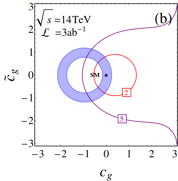
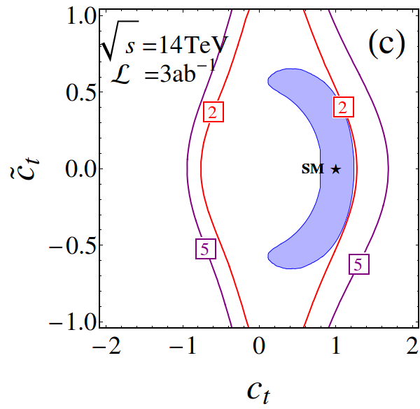
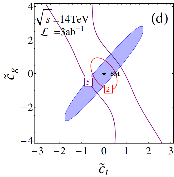
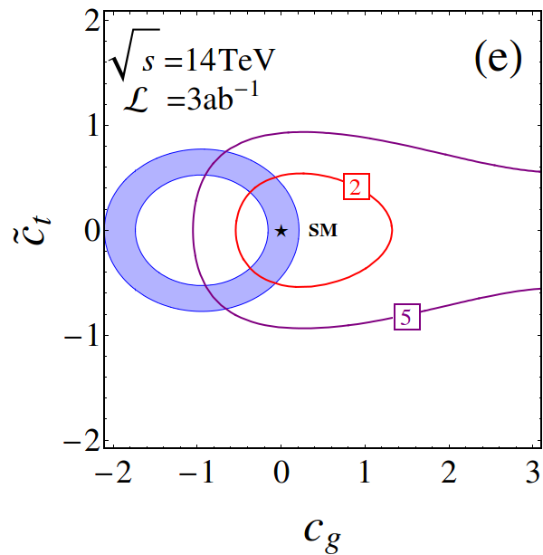
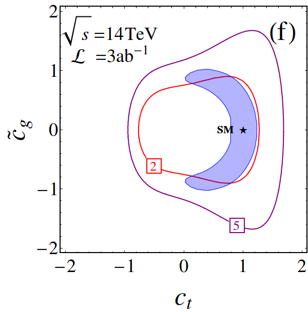
Figure 7: Contours of $2\sigma$ exclusion (red curves) and $5\sigma$ discovery (purple curves) for different combinations of Higgs effective couplings at the HL-LHC. The blue regions represent the $95\%$ CL constraints at the 7 and 8 TeV LHC.

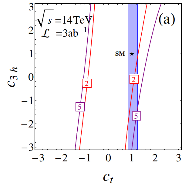
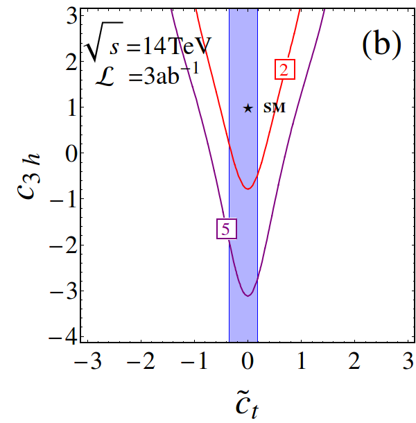
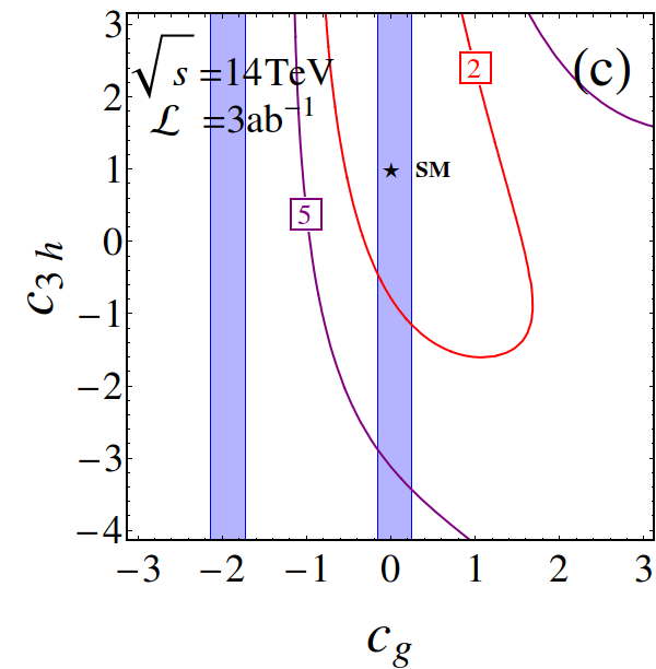
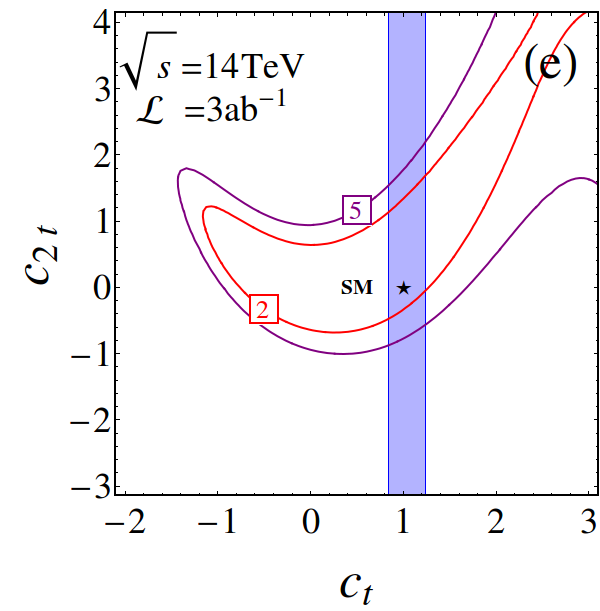
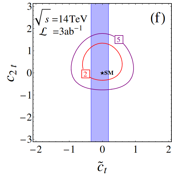
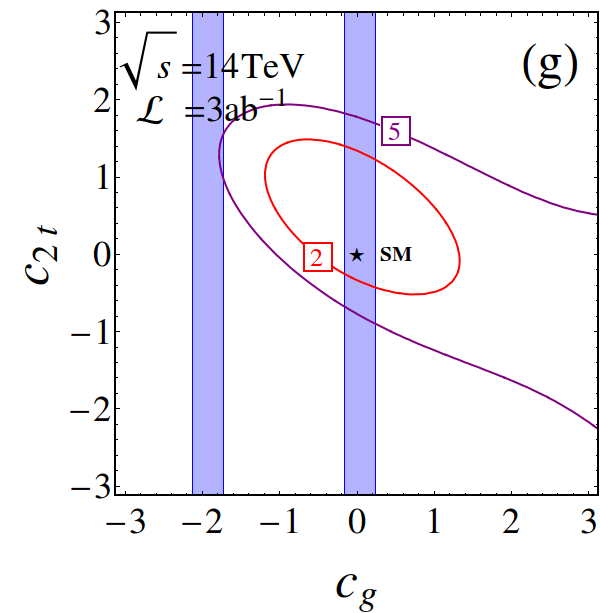
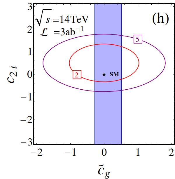
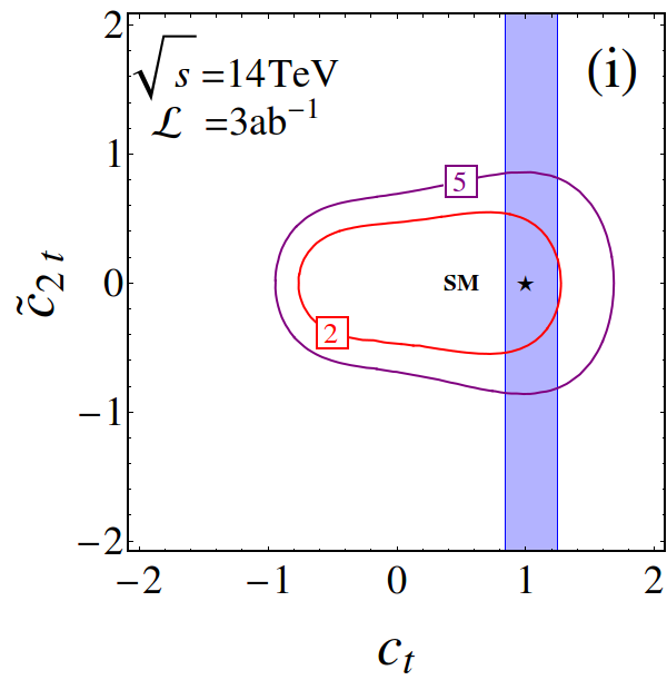
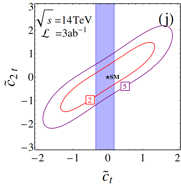
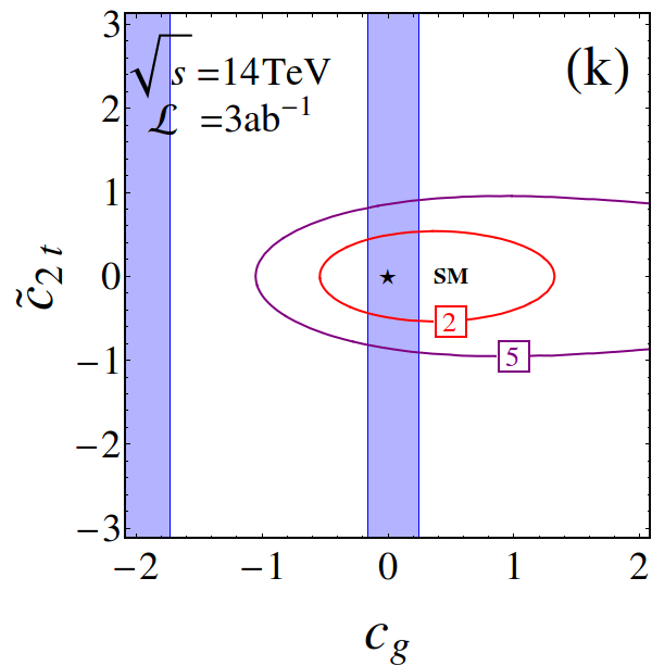
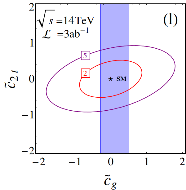
Figure 8: Contours of $2\sigma$ exclusion (red curves) and $5\sigma$ discovery (purple curves) for different combinations of Higgs effective couplings at the HL-LHC. The blue regions represent the $95\%$ CL constraints at the 7 and 8 TeV LHC.

Not all the effective couplings affect the single Higgs production and Higgs boson decay. We separate the effective couplings into two categories: couplings sensitive to single Higgs production, say $c_{t,g}$ and $\tilde{c}_{t,g}$, and others. Figure 8 shows the correlation among $c_{t,g}$ ($\tilde{c}_{t,g}$) and others effective couplings. Plots in the first row in Fig. 8 show the correlations between $c_{3h}$ and $c_{t},\tilde{c}_{t},c_{g},\tilde{c}_{g}$, respectively. The sign of $c_{3h}$ coupling is important as it could alter the cancellation between the triangle diagram and the box diagram in the SM. A negative $c_{3h}$ leads to an enhancement of the double Higgs production, easily yielding a $5\sigma$ discovery. On the other hand, the $2\sigma$ exclusion limit demands the $c_{3h}$ being not too negatively large when $c_{t}=1$; see Figs. 8(b), (c) and (d). The tension is slightly alleviated in $(c_{3h},c_{t})$; it requires $c_{3h}>-2$ if the double Higgs event is not observed at the HL-LHC; see Fig. 8(a). There is no stringent bound on $c_{3h}$ from top, indicating that the double Higgs production is not sensitive to the quartic term in the Higgs potential if the coefficient is positive. It has been pointed out in the comprehensive study in Ref. Azatov et al. (2015) which considers the CP-conserving operators. Our study shows the conclusion also holds for a CP-violating model.

Plots in the second (third) row of Fig. 8 show the correlations between $c_{2t}(\tilde{c}_{2t})$ and $c_{t},\tilde{c}_{t},c_{g},\tilde{c}_{g}$, respectively. If the NP model generates a sizable $c_{2t}$, then it is very promising to see its effects in the Higgs boson pair productions in both CP-conserving and CP-violating models; see the purple curves. Similar to the case of $c_{3h}$, the cancellation between $F_{\triangle}$ and $F_{\Box}$ also imposes a bound on $c_{2t}$ from bottom. Unlike the $c_{3h}$, the $c_{t}$ coupling is also bounded from top. If no deviation is observed in the double Higgs production, then one can impose a bound on $c_{2t}$ ($\tilde{c}_{2t}$), together with constraints obtained from the single Higgs production, as follows:

$$(c_{t},c_{2t}):-0.469\lesssim c_{2t}\lesssim 1.69, (c_{t},\tilde{c}_{2t}):-0.545\lesssim\tilde{c}_{2t}\lesssim 0.542,$$

$$(\tilde{c}_{t},c_{2t}):-0.339\lesssim c_{2t}\lesssim 1.34, (\tilde{c}_{t},\tilde{c}_{2t}):-0.817\lesssim\tilde{c}_{2t}\lesssim 0.671,$$

$$(c_{g},c_{2t}):-0.429\lesssim c_{2t}\lesssim 1.40, (c_{g},\tilde{c}_{2t}):-0.546\lesssim\tilde{c}_{2t}\lesssim 0.529,$$

$$(\tilde{c}_{g},c_{2t}):-0.339\lesssim c_{2t}\lesssim 1.34, (\tilde{c}_{g},\tilde{c}_{2t}):-0.519\lesssim\tilde{c}_{2t}\lesssim 0.516~{}.$$ (68)

It is worth mentioning that the degenerate parameter spaces in $c_{g}$, i.e. the two blue bands in Figs. 8 (c), (g) and (k), can be fully resolved at the HL-LHC.

Figure 9 shows the correlations among effective couplings ($c_{2t}$, $\tilde{c}_{2t}$ and $c_{3h}$) that do not affect the single Higgs production. The three couplings are completely free. They are constrained only by double Higgs production at the HL-LHC. If the NP effects are hidden in the three couplings, then one is not able to probe the NP effects no matter how accurately one measures the single Higgs boson production. The double Higgs production is sensitive to both magnitude and sign of the $c_{3h}$ coupling. If $c_{3h}$ is the only non-zero effective coupling, then null results of Higgs pair searches will require $c_{3h}>-1$. Including $c_{2t}$ completely relax the constraint on $c_{3h}$; see Fig. 9(a). It is owing to the interference between $c_{3h}F_{\triangle}$ and $c_{2t}F_{\triangle}$ terms in Eq. (16). As a result, a large negative $c_{3h}$ is still allowed. The $\tilde{c}_{2t}$ coupling, which does not interfere with $c_{3h}$, has no strong impact on $c_{3h}$. The $c_{2t}$ and $\tilde{c}_{2t}$ do not interfere and result in the symmetric eclipse bound.

Finally, we list analytical expressions of all the $2\sigma$ exclusion limits below:

$$(c_{t},c_{g}):\ 2.25c_{g}^{2}+c_{g}(0.508-1.15c_{t})c_{t}+1.64c_{t}^{4}-0.739c_{t}^{3}+0.0993c_{t}^{2}-1.00<1.28~{},$$

$$(c_{g},\tilde{c}_{g}):\ 2.25c_{g}^{2}-0.645c_{g}+2.25\tilde{c}_{g}^{2}<1.28~{},$$

$$(c_{t},\tilde{c}_{t}):1.64c_{t}^{4}-0.739c_{t}^{3}+c_{t}^{2}(7.18\tilde{c}_{t}^{2}+0.0993)-2.46c_{t}\tilde{c}_{t}^{2}+0.571\tilde{c}_{t}^{4}+0.257\tilde{c}_{t}^{2}-1.00<1.28~{},$$

$$(\tilde{c}_{t},\tilde{c}_{g}):\ 2.25\tilde{c}_{g}^{2}+1.72\tilde{c}_{g}\tilde{c}_{t}+0.571\tilde{c}_{t}^{4}+4.97\tilde{c}_{t}^{2}<1.28~{},$$

$$(c_{g},\tilde{c}_{t}):\ 2.25c_{g}^{2}+c_{g}(1.65\tilde{c}_{t}^{2}-0.645)+0.571\tilde{c}_{t}^{4}+4.97\tilde{c}_{t}^{2}<1.28~{},$$

$$(c_{t},\tilde{c}_{g}):\ 2.25\tilde{c}_{g}^{2}+1.64c_{t}^{4}-0.739c_{t}^{3}+0.0993c_{t}^{2}-1.00<1.28~{},$$

$$(c_{t},c_{3h}):\ 0.0993c_{3h}^{2}c_{t}^{2}-0.739c_{3h}c_{t}^{3}+1.64c_{t}^{4}-1.00<1.28~{},$$

$$(\tilde{c}_{t},c_{3h}):\ c_{3h}^{2}(0.257\tilde{c}_{t}^{2}+0.0993)+c_{3h}(-2.46\tilde{c}_{t}^{2}-0.739)+0.571\tilde{c}_{t}^{4}+7.18\tilde{c}_{t}^{2}+0.639<1.28~{},$$

$$(c_{g},c_{3h}):\ c_{3h}^{2}(0.0369c_{g}^{2}+0.0975c_{g}+0.0993)+c_{3h}(0.406c_{g}^{2}+0.146c_{g}-0.739)+1.80c_{g}^{2}-0.888c_{g}+0.639<1.28~{},$$

$$(\tilde{c}_{g},c_{3h}):\ c_{3h}^{2}(0.0369\tilde{c}_{g}^{2}+0.0993)+c_{3h}(0.406\tilde{c}_{g}^{2}-0.739)+1.80\tilde{c}_{g}^{2}+0.639<1.28~{},$$

$$(c_{t},c_{2t}):\ 2.85c_{2t}^{2}+c_{2t}(0.920-3.79c_{t})c_{t}+1.64c_{t}^{4}-0.739c_{t}^{3}+0.0993c_{t}^{2}-1.00<1.28~{},$$

$$(\tilde{c}_{t},c_{2t}):\ 2.85c_{2t}^{2}+c_{2t}(1.91\tilde{c}_{t}^{2}-2.87)+0.571\tilde{c}_{t}^{4}+4.97\tilde{c}_{t}^{2}<1.28~{},$$

$$(c_{g},c_{2t}):\ 2.85c_{2t}^{2}+c_{2t}(2.52c_{g}-2.87)+2.25c_{g}^{2}-0.645c_{g}<1.28~{},$$

$$(\tilde{c}_{g},c_{2t}):\ 2.85c_{2t}^{2}-2.87c_{2t}+2.25\tilde{c}_{g}^{2}<1.28~{},$$

$$(c_{t},\tilde{c}_{2t}):\ 5.28\tilde{c}_{2t}^{2}+1.64c_{t}^{4}-0.739c_{t}^{3}+0.0993c_{t}^{2}-1.00<1.28~{},$$

$$(\tilde{c}_{t},\tilde{c}_{2t}):\ 5.28\tilde{c}_{2t}^{2}-10.2\tilde{c}_{2t}\tilde{c}_{t}+0.571\tilde{c}_{t}^{4}+4.97\tilde{c}_{t}^{2}<1.28~{},$$

$$(c_{g},\tilde{c}_{2t}):\ 5.28\tilde{c}_{2t}^{2}+2.25c_{g}^{2}-0.645c_{g}<1.28~{},$$

$$(\tilde{c}_{g},\tilde{c}_{2t}):\ 5.28\tilde{c}_{2t}^{2}-2.07\tilde{c}_{2t}\tilde{c}_{g}+2.25\tilde{c}_{g}^{2}<1.28~{},$$

$$(c_{3h},c_{2t}):\ 2.85c_{2t}^{2}+c_{2t}(0.920c_{3h}-3.79)+0.0993c_{3h}^{2}-0.739c_{3h}+0.639<1.28~{},$$

$$(c_{3h},\tilde{c}_{2t}):\ 5.28\tilde{c}_{2t}^{2}+0.0993c_{3h}^{2}-0.739c_{3h}+0.639<1.28~{},$$

$$(c_{2t},\tilde{c}_{2t}):\ 2.85c_{2t}^{2}-2.87c_{2t}+5.28\tilde{c}_{2t}^{2}<1.28~{}.$$ (69)

Effective couplings violating the above inequalities can be excluded at the HL-LHC.

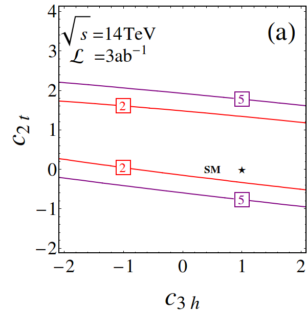
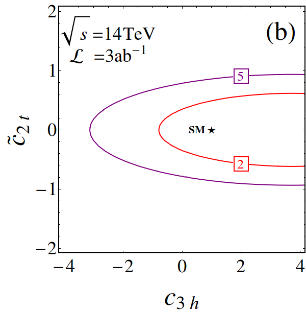
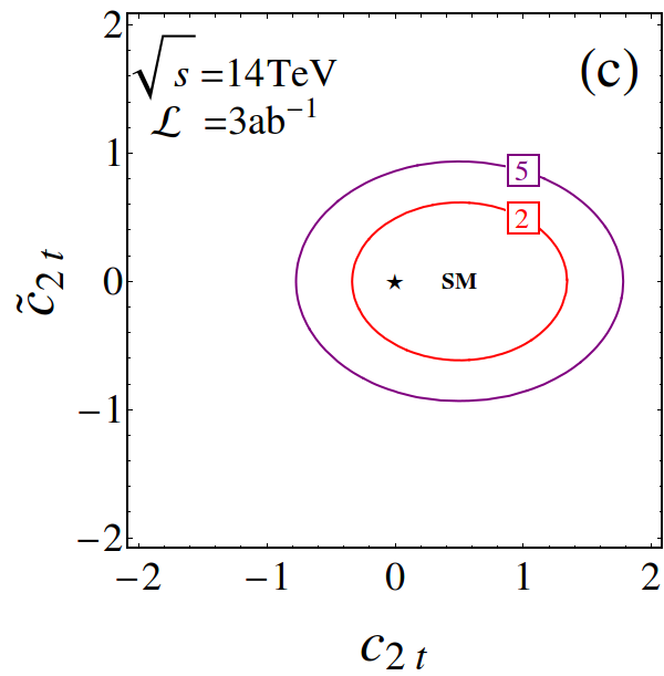
Figure 9: Contours of $2\sigma$ exclusion (red curves) and $5\sigma$ discovery (purple curves) for different combinations of Higgs effective couplings at the HL-LHC.

IV.5 Sensitivity to Higgs effective couplings at a future 100 TeV $pp$-collider

Now we study the potential of a future 100 TeV $pp$-collider on Higgs effective couplings. It is shown that increasing the collider energy improves the sensitivity significantly Azatov et al. (2015); Contino et al. (2016). Our simulation shows that the performance at the 100 TeV machine with an integrated luminosity of $10~{}\rm fb^{-1}$ is comparable to that at the HL-LHC. Moreover, the $gg\to hh\to b\bar{b}\gamma\gamma$ process can be discovered with $\mathcal{L}=256~{}\rm fb^{-1}$ at the 100 TeV $pp$-collider. Accumulating more luminosity enables us to discover NP effects in the double Higgs productions through $b\bar{b}\gamma\gamma$ channel.

As it is guaranteed to observe the Higgs pair signal in the SM at the 100 TeV machine, we focus on the NP searches hereafter. Figures 10-13 display the $5\sigma$ contours of discovering NP with an integrated luminosity of $30~{}\rm ab^{-1}$. The SM process $gg\to hh\to b\bar{b}\gamma\gamma$ is recognized as a background. The regions with the significance $Z_{0}<5$ are depicted with magenta curves. Outside of those magenta regions, the NP is expected to be observed. Again the constraints from the current single Higgs measurements are denoted in blue regions. We also include the EDM constraints on the CP-odd couplings $\tilde{c}_{t}$ and $\tilde{c}_{g}$; see the grey bands. The EDM constraints are very strigent on $\tilde{c}_{t}$ or $\tilde{c}_{g}$. The double Higgs production provides an alternative way to check $\tilde{c}_{t}$ and $\tilde{c}_{g}$. If the Higgs pair signal in the NP model is discovered in the parameter space outside the EDM bound, then additional CP-violating interaction has to be included to respect the EDM constraint.

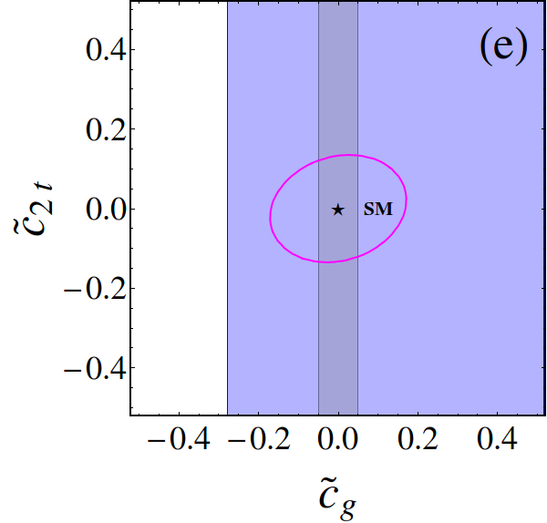
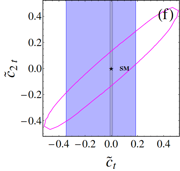
Figure 10: $5\sigma$ discovery contours for different combinations of Higgs effective couplings at the 100 TeV $pp$-collider with the integrated luminosity $\mathcal{L}=30~{}\rm ab^{-1}$. The blue regions represent the $95\%$ CL constraints at the 7 and 8 TeV LHC.

We classify those figures into four categories according to the shapes of the boundary of $5\sigma$ discovery region. All the discovery regions in Fig. 10 are in a shape of ellipse; see the magenta curve. The parameter outside those ellipses can be discovered at more than $5\sigma$ confidence level. In the parameter space that is close to the SM, the modification of the decay branching ratios $\mu_{\gamma\gamma}$ and $\mu_{b\bar{b}}$ can be ignored. We obtain analytic expressions corresponding to the $5\sigma$ discovery of NP effects as follows:

$$(c_{g},\tilde{c}_{g}):~{}~{}3.70c_{g}^{2}-0.290c_{g}+3.70\tilde{c}_{g}^{2}\geq 0.1~{},$$

$$(\tilde{c}_{g},\tilde{c}_{t}):~{}~{}3.70\tilde{c}_{g}^{2}+1.40\tilde{c}_{g}\tilde{c}_{t}+0.806\tilde{c}_{t}^{4}+4.54\tilde{c}_{t}^{2}\geq 0.1~{},$$

$$(c_{g},\tilde{c}_{t}):~{}~{}3.70c_{g}^{2}+c_{g}(1.90\tilde{c}_{t}^{2}-0.290)+0.806\tilde{c}_{t}^{4}+4.54\tilde{c}_{t}^{2}\geq 0.1~{},$$

$$(c_{g},\tilde{c}_{2t}):\ 5.68\tilde{c}_{2t}^{2}+3.70c_{g}^{2}-0.290c_{g}\geq 0.1~{},$$

$$(\tilde{c}_{g},\tilde{c}_{2t}):\ 5.68\tilde{c}_{2t}^{2}-1.46\tilde{c}_{2t}\tilde{c}_{g}+3.70\tilde{c}_{g}^{2}\geq 0.1~{},$$

$$(\tilde{c}_{t},\tilde{c}_{2t}):\ 5.68\tilde{c}_{2t}^{2}-9.73\tilde{c}_{2t}\tilde{c}_{t}+0.806\tilde{c}_{t}^{4}+4.54\tilde{c}_{t}^{2}\geq 0.1~{}.$$ (70)

The analytical expressions of one effective coupling can be derived from the above inequalities by setting the other coupling to be zero. The $5\sigma$ curve in $(\tilde{c}_{t},\tilde{c}_{2t})$ is stretched as a result of the significant interference effect between $\tilde{c}_{t}F_{\Box}^{(2)}$ and $\tilde{c}_{2t}F_{\triangle}^{(1)}$.

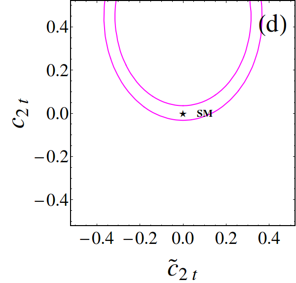
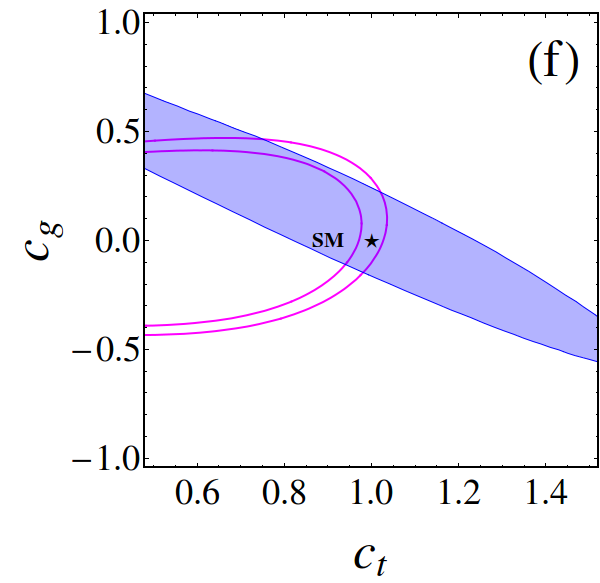
Figure 11: $5\sigma$ discovery contours for different combinations of Higgs effective couplings at the 100 TeV $pp$-collider with the integrated luminosity $\mathcal{L}=30~{}\rm ab^{-1}$. The blue regions represent the $95\%$ CL constraints at the 7 and 8 TeV LHC.

Figure 11 displays the correlation among effective couplings, of which the $5\sigma$ discovery boundary exhibits a ring type shape. Most of parameter space allowed by the single Higgs production can be covered by double Higgs production. The parameter outside the $5\sigma$ band produces more Higgs pair events, while the parameter inside the band reduces Higgs pair events. The bands of discovery potential at a confidence level less than $5\sigma$ are listed as follows:

$$(c_{g},c_{2t}):\ ~{}-0.1<3.33c_{2t}^{2}+c_{2t}(2.33c_{g}-2.98)+3.70c_{g}^{2}-0.290c_{g}<0.1,$$

$$(\tilde{c}_{g},c_{2t}):\ ~{}-0.1<3.33c_{2t}^{2}-2.98c_{2t}+3.70\tilde{c}_{g}^{2}<0.1,$$

$$(\tilde{c}_{t},c_{2t}):\ ~{}-0.1<3.33c_{2t}^{2}+c_{2t}(1.92\tilde{c}_{t}^{2}-2.98)+0.806\tilde{c}_{t}^{4}+4.54\tilde{c}_{t}^{2}<0.1,$$

$$(\tilde{c}_{2t},c_{2t}):\ -0.1<3.33c_{2t}^{2}-2.98c_{2t}+5.68\tilde{c}_{2t}^{2}<0.1,$$

$$(c_{t},\tilde{c}_{2t}):\ ~{}-0.1<5.68\tilde{c}_{2t}^{2}+1.58c_{t}^{4}-0.671c_{t}^{3}+0.0880c_{t}^{2}-1.00<0.1,$$

$$(c_{t},c_{g}):\ ~{}-0.1<3.70c_{g}^{2}+c_{g}(0.457-0.746c_{t})c_{t}+1.58c_{t}^{4}-0.671c_{t}^{3}+0.0880c_{t}^{2}-1.00<0.1,$$

$$(c_{t},\tilde{c}_{t}):\ ~{}-0.1<1.58c_{t}^{4}-0.671c_{t}^{3}+c_{t}^{2}(6.46\tilde{c}_{t}^{2}+0.0880)-2.14c_{t}\tilde{c}_{t}^{2}+0.806\tilde{c}_{t}^{4}+0.222\tilde{c}_{t}^{2}-1.00<0.1,$$

$$(c_{t},\tilde{c}_{g}):\ ~{}-0.1<3.70\tilde{c}_{g}^{2}+1.58c_{t}^{4}-0.671c_{t}^{3}+0.0880c_{t}^{2}-1.00<0.1~{}.$$ (71)

Couplings violating the above inequalities lead to a discovery of Higgs pair signal in the NP model.

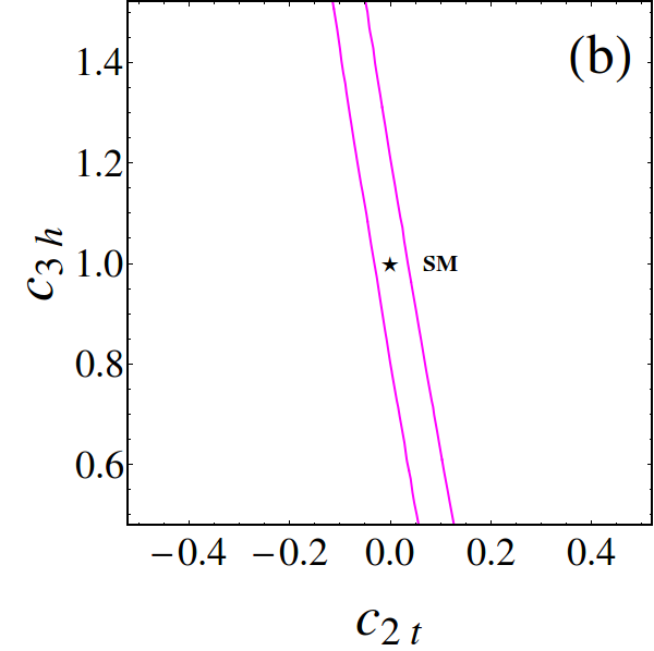
Figure 12: $5\sigma$ discovery contours for different combinations of Higgs effective couplings at the 100 TeV $pp$-collider with the integrated luminosity $\mathcal{L}=30~{}\rm ab^{-1}$. The blue regions represent the $95\%$ CL constraints at the 7 and 8 TeV LHC.

Figure 12 displays the $5\sigma$ contour with a line shape. We notice that, owing to the insensitivity to $c_{3h}$, the $5\sigma$ discovery band in $(c_{t},c_{3h})$ and $(c_{2t},c_{3h})$ appears as a vertical line. The $5\sigma$ band in $(c_{t},c_{2t})$ is determined by the cancellation among $c_{t}^{2}F_{\Box}$ and $c_{2t}F_{\triangle}$ terms. The bands of discovery potential at a confidence level less than $5\sigma$ are

$$(c_{t},c_{3h}):\ ~{}-0.1<0.0880c_{3h}^{2}c_{t}^{2}-0.671c_{3h}c_{t}^{3}+1.58c_{t}^{4}-1.00<0.1,$$

$$(c_{2t},c_{3h}):\ -0.1<3.33c_{2t}^{2}+c_{2t}(0.889c_{3h}-3.87)+0.0880c_{3h}^{2}-0.671c_{3h}+0.583<0.1,$$

$$(c_{t},c_{2t}):\ ~{}-0.1<3.33c_{2t}^{2}+c_{2t}(0.889-3.87c_{t})c_{t}+1.58c_{t}^{4}-0.671c_{t}^{3}+0.0880c_{t}^{2}-1.00<0.1~{}.$$ (72)

Finally, we plot in Fig. 13 the $5\sigma$ contour with a irregular shape. The bands of discovery potential at a confidence level less than $5\sigma$ are

$$(\tilde{c}_{t},c_{3h}):\ -0.1<c_{3h}^{2}(0.222\tilde{c}_{t}^{2}+0.0880)+c_{3h}(-2.14\tilde{c}_{t}^{2}-0.671)+0.806\tilde{c}_{t}^{4}+6.46\tilde{c}_{t}^{2}+0.583<0.1~{},$$

$$(c_{g},c_{3h}):\ -0.1<c_{3h}^{2}(0.0347c_{g}^{2}+0.0846c_{g}+0.0880)+c_{3h}(0.465c_{g}^{2}+0.157c_{g}-0.671)+3.20c_{g}^{2}-0.531c_{g}+0.583<0.1~{},$$

$$(\tilde{c}_{g},c_{3h}):\ -0.1<c_{3h}^{2}(0.0347\tilde{c}_{g}^{2}+0.0880)+c_{3h}(0.465\tilde{c}_{g}^{2}-0.671)+3.20\tilde{c}_{g}^{2}+0.583<0.1~{},$$

$$(\tilde{c}_{2t},c_{3h}):\ -0.1<5.68\tilde{c}_{2t}^{2}+0.0880c_{3h}^{2}-0.671c_{3h}+0.583<0.1~{}.$$ (73)

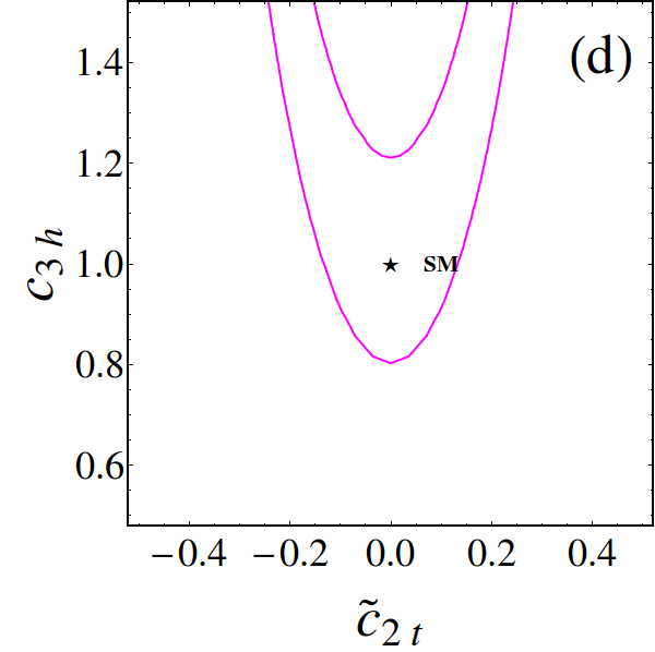
Figure 13: $5\sigma$ discovery contours for different combinations of Higgs effective couplings at the 100 TeV $pp$-collider with the integrated luminosity $\mathcal{L}=30~{}\rm ab^{-1}$. The blue regions represent the $95\%$ CL constraints at the 7 and 8 TeV LHC.

V Conclusions

We considered effective Higgs boson couplings that affect the double Higgs production. For generality we included both CP-even and CP-odd effective couplings. Some of the effective couplings are loosely constrained by the single Higgs measurements at the 7 TeV and the 8 TeV LHC. The correlations of those effective couplings are different in single and double Higgs productions, therefore, one can probe those effective couplings by combining both the single and double Higgs productions. We examined the impact of the effective couplings on double Higgs production at the high luminosity LHC with an integrated luminosity of $3000~{}{\rm fb}^{-1}$ and at a future $pp$-collider operating at an energy of 100 TeV with an integrated luminosity of $30~{}\rm{ab}^{-1}$.

The amplitude of the double Higgs production depends on several form factors. From partial wave analysis, we found that the double Higgs production is still dominated by the $s$-wave component even at the 100 $pp$-collider. Making use of the $s$-wave dominant feature, we propose a universal cut efficiency function $\mathcal{A}({m}_{hh})$ to mimic the experimental cuts and detector effects. Convoluting inclusive distribution of the invariant mass of Higgs pair with the cut efficiency function gives rise to the signal events after experimental cuts. We followed the analysis in Refs.ATLAS Collaboration (2015a); Contino et al. (2016) to derive the cut efficiency functions at the 14 TeV LHC and the 100 TeV $pp$-collider. Using the cut efficiency functions, we obtain the differential cross sections of $m_{hh}$ and total cross sections of $gg\to hh\to b\bar{b}\gamma\gamma$ after kinematics cuts. From there we obtained the potential of probing those effective couplings at the 14 TeV HL-LHC and at the 100 TeV $pp$-collider.

We varied two effective couplings at a time and fixed other couplings to be the SM values. With the tremendously high luminosity, the HL-LHC could cover a lot of parameter space, which could yield a $5\sigma$ discovery. Negative results of Higgs pair searches also exclude a vast amount of parameter spaces. There are two islands in the parameter space of $(c_{t},c_{g})$, $(c_{g},c_{3h})$, $(c_{g},c_{2t})$ and $(c_{g},\tilde{c}_{2t})$, which cannot be resolved by the single Higgs production. The double Higgs production could exclude the island that does not consist of the SM. We also presented the analytical expressions of those $2\sigma$ exclusion limits in the parameter space.

We found that the double Higgs production can be discovered in the process $gg\to hh\to b\bar{b}\gamma\gamma$ at the 100 TeV $pp$-collider with an integrated luminosity of $256~{}{\rm fb}^{-1}$. We thus focused on searching for Higgs effective couplings at the 100 TeV machine with $\mathcal{L}=30~{}\rm{ab}^{-1}$ and treat the SM double Higgs production as a background. Thanks to the large center of mass energy, the 100 TeV $pp$-collider could cover almost entire parameter space of effective couplings, except $c_{3h}$ which is not sensitive to the Higgs pair production. Finally, we listed analytical expressions of the $5\sigma$ discovery bands which, together with the analytical expressions of the $2\sigma$ exclusion limits at the HL-LHC, is useful to probe new physics models.

Appendix A The expressions of form factors

In this appendix, we collect the explicit expressions of the form factors in the single and double Higgs productions,

$$F_{\Box} = \frac{2m_{t}^{2}}{\hat{s}}\{m_{t}^{2}(8m_{t}^{2}-\hat{s}-2m_{h}^{2})(D_{0}^{t}+D_{0}^{u}+D_{0}^{tu})+p_{T}^{2}(4m_{t}^{2}-m_{h}^{2})D_{0}^{tu}$$ (74)

$$+2+4m_{t}^{2}C_{0}^{s}+\frac{2}{\hat{s}}(m_{h}^{2}-4m_{t}^{2})[(\hat{t}-m_{h}^{2})C_{0}^{t}+(\hat{u}-m_{h}^{2})C_{0}^{u}]\},$$

$$G_{\Box} = \frac{m_{t}^{2}}{\hat{s}}\{2(8m_{t}^{2}+\hat{s}-2m_{h}^{2})[m_{t}^{2}(D_{0}^{t}+D_{0}^{u}+D_{0}^{tu})-C_{0}^{sm}]-2[\hat{s}C_{0}^{s}+(\hat{t}-m_{h}^{2})C_{0}^{t}+(\hat{u}-m_{h}^{2})C_{0}^{u}]$$ (75)

$$+\frac{1}{\hat{s}p_{T}^{2}}[\hat{s}\hat{u}(8\hat{u}m_{t}^{2}-\hat{u}^{2}-m_{h}^{4})D_{0}^{u}+\hat{s}\hat{t}(8\hat{t}m_{t}^{2}-\hat{t}^{2}-m_{h}^{4})D_{0}^{t}+(8m_{t}^{2}+\hat{s}-m_{h}^{2})$$

$$[\hat{s}(\hat{s}-2m_{h}^{2})C_{0}^{s}+\hat{s}(\hat{s}-4m_{h}^{2})C_{0}^{sm}+2\hat{t}(m_{h}^{2}-\hat{t})C_{0}^{t}+2\hat{u}(m_{h}^{2}-\hat{u})C_{0}^{u}]]\},$$

$$F_{\Box}^{(1)} = \frac{2m_{t}^{2}}{\hat{s}^{2}}\{m_{h}^{2}(2\hat{t}C_{0}^{t}+2\hat{u}C_{0}^{u}-\hat{t}\hat{u}D_{0}^{tu})-2m_{h}^{4}(C_{0}^{t}+C_{0}^{u})+m_{h}^{6}D_{0}^{tu}$$ (76)

$$+\hat{s}[2+m_{t}^{2}[4C_{0}^{s}-(D_{0}^{t}+D_{0}^{u}+D_{0}^{tu})(\hat{t}+\hat{u})]]\}$$

$$G_{\Box}^{(1)} = \frac{m_{t}^{2}}{2\hat{s}}\{\frac{2}{m_{h}^{4}-\hat{t}\hat{u}}[-\hat{s}(2m_{h}^{4}+\hat{t}^{2}+\hat{u}^{2})C_{0}^{s}+2(m_{h}^{2}-\hat{t})(m_{h}^{4}+\hat{t}^{2})C_{0}^{t}+2(m_{h}^{2}-\hat{u})(m_{h}^{4}+\hat{u}^{2})C_{0}^{u}$$ (77)

$$-(\hat{t}+\hat{u})(2m_{h}^{4}-\hat{t}^{2}-\hat{u}^{2})C_{0}^{sm}+\hat{s}\hat{t}(\hat{t}^{2}+m_{h}^{4})D_{0}^{t}+\hat{s}\hat{u}(\hat{u}^{2}+m_{h}^{4})D_{0}^{u}]$$

$$-4m_{t}^{2}(\hat{t}+\hat{u})(D_{0}^{t}+D_{0}^{u}+D_{0}^{tu})\},$$

$$F_{\Box}^{(2)} = 4m_{t}^{4}(D_{0}^{t}+D_{0}^{u}+D_{0}^{tu}),$$ (78)

$$F_{\triangle} = \frac{2m_{t}^{2}}{\hat{s}}[2+(4m_{t}^{2}-s)C_{0}^{s}],$$ (79)

$$F_{\triangle}^{(1)} = 2m_{t}^{2}C_{0}^{s}.$$ (80)

In the above we have the conventions Shao et al. (2013)

$$C_{0}^{s} = C_{0}(0,0,\hat{s},m_{t}^{2},m_{t}^{2},m_{t}^{2}),\ C_{0}^{t}=C_{0}(0,\hat{t},m_{h}^{2},m_{t}^{2},m_{t}^{2},m_{t}^{2}),$$

$$C_{0}^{u} = C_{0}(0,\hat{u},m_{h}^{2},m_{t}^{2},m_{t}^{2},m_{t}^{2}),\ C_{0}^{sm}=C_{0}(m_{h}^{2},\hat{s},m_{h}^{2},m_{t}^{2},m_{t}^{2},m_{t}^{2})$$

$$D_{0}^{t} = D_{0}(m_{h}^{2},0,0,m_{h}^{2},\hat{t},\hat{s},m_{t}^{2},m_{t}^{2},m_{t}^{2},m_{t}^{2}),$$

$$D_{0}^{u} = D_{0}(m_{h}^{2},0,0,m_{h}^{2},\hat{u},\hat{s},m_{t}^{2},m_{t}^{2},m_{t}^{2},m_{t}^{2}),$$

$$D_{0}^{tu} = D_{0}(m_{h}^{2},0,m_{h}^{2},0,\hat{t},\hat{u},m_{t}^{2},m_{t}^{2},m_{t}^{2},m_{t}^{2}),$$ (81)

and the definitions of the scalar Passarino-Veltman functions are as follows Denner (1993)

$$C_{0}(p_{1}^{2},p_{2}^{2},(p_{1}+p_{2})^{2},m_{1}^{2},m_{2}^{2},m_{3}^{2})$$ (82)

$$= \frac{(2\pi\mu)^{4-D}}{i\pi^{2}}\int d^{D}q\frac{1}{(q^{2}-m_{1}^{2})[(q+p_{1})^{2}-m_{2}^{2}][(q+p_{1}+p_{2})^{2}-m_{3}^{2}]},$$

$$D_{0}(p_{1}^{2},p_{2}^{2},p_{3}^{2},p_{4}^{2},(p_{1}+p_{2})^{2},(p_{2}+p_{3})^{2},m_{1}^{2},m_{2}^{2},m_{3}^{2},m_{4}^{2})$$

$$= \frac{(2\pi\mu)^{4-D}}{i\pi^{2}}\int d^{D}q\frac{1}{(q^{2}-m_{1}^{2})[(q+p_{1})^{2}-m_{2}^{2}][(q+p_{1}+p_{2})^{2}-m_{3}^{2}][(q+p_{1}+p_{2}+p_{3})^{2}-m_{4}^{2}]},$$

where $\mu$ is the renormalization scale and $D$ is the space-time dimension.

References

- Glover and van der Bij (1988) E. W. N. Glover and J. J. van der Bij, Nucl. Phys. B309, 282 (1988).
- Baur et al. (2003) U. Baur, T. Plehn, and D. L. Rainwater, Phys. Rev. D68, 033001 (2003), eprint hep-ph/0304015.
- Baur et al. (2004) U. Baur, T. Plehn, and D. L. Rainwater, Phys. Rev. D69, 053004 (2004), eprint hep-ph/0310056.
- Dolan et al. (2012) M. J. Dolan, C. Englert, and M. Spannowsky, JHEP 10, 112 (2012), eprint 1206.5001.
- Baglio et al. (2013) J. Baglio, A. Djouadi, R. Gröber, M. M. Mühlleitner, J. Quevillon, and M. Spira, JHEP 04, 151 (2013), eprint 1212.5581.
- Papaefstathiou et al. (2013) A. Papaefstathiou, L. L. Yang, and J. Zurita, Phys. Rev. D87, 011301 (2013), eprint 1209.1489.
- Barger et al. (2014) V. Barger, L. L. Everett, C. B. Jackson, and G. Shaughnessy, Phys. Lett. B728, 433 (2014), eprint 1311.2931.
- Barr et al. (2014) A. J. Barr, M. J. Dolan, C. Englert, and M. Spannowsky, Phys. Lett. B728, 308 (2014), eprint 1309.6318.
- Yao (2013) W. Yao, in Community Summer Study 2013: Snowmass on the Mississippi (CSS2013) Minneapolis, MN, USA, July 29-August 6, 2013 (2013), eprint 1308.6302, URL https://inspirehep.net/record/1251544/files/arXiv:1308.6302.pdf.
- Ferreira de Lima et al. (2014) D. E. Ferreira de Lima, A. Papaefstathiou, and M. Spannowsky, JHEP 08, 030 (2014), eprint 1404.7139.
- Li et al. (2015) Q. Li, Z. Li, Q.-S. Yan, and X. Zhao, Phys. Rev. D92, 014015 (2015), eprint 1503.07611.
- Agashe et al. (2005) K. Agashe, R. Contino, and A. Pomarol, Nucl. Phys. B719, 165 (2005), eprint hep-ph/0412089.
- Contino et al. (2007) R. Contino, L. Da Rold, and A. Pomarol, Phys. Rev. D75, 055014 (2007), eprint hep-ph/0612048.
- Arkani-Hamed et al. (2001) N. Arkani-Hamed, A. G. Cohen, and H. Georgi, Phys. Lett. B513, 232 (2001), eprint hep-ph/0105239.
- Arkani-Hamed et al. (2002) N. Arkani-Hamed, A. G. Cohen, E. Katz, and A. E. Nelson, JHEP 07, 034 (2002), eprint hep-ph/0206021.
- Buchmuller and Wyler (1986) W. Buchmuller and D. Wyler, Nucl. Phys. B268, 621 (1986).
- Grzadkowski et al. (2010) B. Grzadkowski, M. Iskrzynski, M. Misiak, and J. Rosiek, JHEP 10, 085 (2010), eprint 1008.4884.
- Contino et al. (2013) R. Contino, M. Ghezzi, C. Grojean, M. Muhlleitner, and M. Spira, JHEP 07, 035 (2013), eprint 1303.3876.
- Pierce et al. (2007) A. Pierce, J. Thaler, and L.-T. Wang, JHEP 05, 070 (2007), eprint hep-ph/0609049.
- Contino et al. (2012) R. Contino, M. Ghezzi, M. Moretti, G. Panico, F. Piccinini, and A. Wulzer, JHEP 08, 154 (2012), eprint 1205.5444.
- Chen and Low (2014) C.-R. Chen and I. Low, Phys. Rev. D90, 013018 (2014), eprint 1405.7040.
- Goertz et al. (2015) F. Goertz, A. Papaefstathiou, L. L. Yang, and J. Zurita, JHEP 04, 167 (2015), eprint 1410.3471.
- Azatov et al. (2015) A. Azatov, R. Contino, G. Panico, and M. Son, Phys. Rev. D92, 035001 (2015), eprint 1502.00539.
- Dawson et al. (2015) S. Dawson, A. Ismail, and I. Low, Phys. Rev. D91, 115008 (2015), eprint 1504.05596.
- Peccei and Quinn (1977) R. D. Peccei and H. R. Quinn, Phys. Rev. Lett. 38, 1440 (1977).
- Djouadi (2008a) A. Djouadi, Phys. Rept. 457, 1 (2008a), eprint hep-ph/0503172.
- Djouadi (2008b) A. Djouadi, Phys. Rept. 459, 1 (2008b), eprint hep-ph/0503173.
- Plehn et al. (1996) T. Plehn, M. Spira, and P. M. Zerwas, Nucl. Phys. B479, 46 (1996), [Erratum: Nucl. Phys.B531,655(1998)], eprint hep-ph/9603205.
- Andersen et al. (2013) J. R. Andersen et al. (LHC Higgs Cross Section Working Group) (2013), eprint 1307.1347.
- The ATLAS and CMS Collaborations (2015) The ATLAS and CMS Collaborations, Tech. Rep. ATLAS-CONF-2015-044 (2015).
- CMS Collaboration (2015a) CMS Collaboration (CMS), Tech. Rep. CMS-PAS-HIG-15-002 (2015a).
- Aad et al. (2016) G. Aad et al. (ATLAS, CMS), JHEP 08, 045 (2016), eprint 1606.02266.
- CMS Collaboration (2016a) CMS Collaboration (CMS), Tech. Rep. CMS-PAS-HIG-16-020 (2016a).
- The ATLAS collaboration (2016) The ATLAS collaboration (ATLAS), Tech. Rep. ATLAS-CONF-2016-067 (2016).
- Brod et al. (2013) J. Brod, U. Haisch, and J. Zupan, JHEP 11, 180 (2013), eprint 1310.1385.
- Chien et al. (2015) Y. T. Chien, V. Cirigliano, W. Dekens, J. de Vries, and E. Mereghetti (2015), eprint 1510.00725.
- Shifman et al. (1979) M. A. Shifman, A. I. Vainshtein, M. B. Voloshin, and V. I. Zakharov, Sov. J. Nucl. Phys. 30, 711 (1979), [Yad. Fiz.30,1368(1979)].
- Kniehl and Spira (1995) B. A. Kniehl and M. Spira, Z. Phys. C69, 77 (1995), eprint hep-ph/9505225.
- Eboli et al. (1987) O. J. P. Eboli, G. C. Marques, S. F. Novaes, and A. A. Natale, Phys. Lett. B197, 269 (1987).
- Dawson et al. (1998) S. Dawson, S. Dittmaier, and M. Spira, Phys. Rev. D58, 115012 (1998), eprint hep-ph/9805244.
- Grigo et al. (2013) J. Grigo, J. Hoff, K. Melnikov, and M. Steinhauser, Nucl. Phys. B875, 1 (2013), eprint 1305.7340.
- Frederix et al. (2014) R. Frederix, S. Frixione, V. Hirschi, F. Maltoni, O. Mattelaer, P. Torrielli, E. Vryonidou, and M. Zaro, Phys. Lett. B732, 142 (2014), eprint 1401.7340.
- Maltoni et al. (2014) F. Maltoni, E. Vryonidou, and M. Zaro, JHEP 11, 079 (2014), eprint 1408.6542.
- Borowka et al. (2016a) S. Borowka, N. Greiner, G. Heinrich, S. Jones, M. Kerner, J. Schlenk, U. Schubert, and T. Zirke, Phys. Rev. Lett. 117, 012001 (2016a), [Erratum: Phys. Rev. Lett.117,no.7,079901(2016)], eprint 1604.06447.
- Borowka et al. (2016b) S. Borowka, N. Greiner, G. Heinrich, S. P. Jones, M. Kerner, J. Schlenk, and T. Zirke (2016b), eprint 1608.04798.
- Kerner (2016) M. Kerner, PoS LL2016, 023 (2016), eprint 1608.03851.
- Ferrera and Pires (2016) G. Ferrera and J. Pires (2016), eprint 1609.01691.
- de Florian and Mazzitelli (2013a) D. de Florian and J. Mazzitelli, Phys. Lett. B724, 306 (2013a), eprint 1305.5206.
- de Florian and Mazzitelli (2013b) D. de Florian and J. Mazzitelli, Phys. Rev. Lett. 111, 201801 (2013b), eprint 1309.6594.
- Grigo et al. (2014) J. Grigo, K. Melnikov, and M. Steinhauser, Nucl. Phys. B888, 17 (2014), eprint 1408.2422.
- Grigo et al. (2015) J. Grigo, J. Hoff, and M. Steinhauser, Nucl. Phys. B900, 412 (2015), eprint 1508.00909.
- Degrassi et al. (2016) G. Degrassi, P. P. Giardino, and R. Gröber, Eur. Phys. J. C76, 411 (2016), eprint 1603.00385.
- de Florian et al. (2016) D. de Florian, M. Grazzini, C. Hanga, S. Kallweit, J. M. Lindert, P. Maierhöfer, J. Mazzitelli, and D. Rathlev, JHEP 09, 151 (2016), eprint 1606.09519.
- Hoff (2016) J. Hoff, PoS LL2016, 024 (2016), eprint 1606.05847.
- Shao et al. (2013) D. Y. Shao, C. S. Li, H. T. Li, and J. Wang, JHEP 07, 169 (2013), eprint 1301.1245.
- de Florian and Mazzitelli (2015) D. de Florian and J. Mazzitelli, JHEP 09, 053 (2015), eprint 1505.07122.
- Cao et al. (2015) Q.-H. Cao, B. Yan, D.-M. Zhang, and H. Zhang (2015), eprint 1508.06512.
- ATLAS Collaboration (2015a) ATLAS Collaboration, Tech. Rep. ATL-PHYS-PUB-2014-019 (2015a).
- Contino et al. (2016) R. Contino et al. (2016), eprint 1606.09408.
- Aad et al. (2015a) G. Aad et al. (ATLAS), Phys. Rev. Lett. 114, 081802 (2015a), eprint 1406.5053.
- Aad et al. (2015b) G. Aad et al. (ATLAS), Phys. Rev. D92, 092004 (2015b), eprint 1509.04670.
- Aad et al. (2015c) G. Aad et al. (ATLAS), Eur. Phys. J. C75, 412 (2015c), eprint 1506.00285.
- CMS Collaboration (2014) CMS Collaboration, Tech. Rep. CMS-PAS-HIG-13-032 (2014).
- Khachatryan et al. (2015a) V. Khachatryan et al. (CMS), Phys. Lett. B749, 560 (2015a), eprint 1503.04114.
- CMS Collaboration (2016b) CMS Collaboration (CMS), Tech. Rep. CMS-PAS-HIG-15-013 (2016b).
- Khachatryan et al. (2016) V. Khachatryan et al. (CMS), Phys. Lett. B755, 217 (2016), eprint 1510.01181.
- The ATLAS Collaboration (2016) The ATLAS Collaboration, Tech. Rep. ATLAS-CONF-2016-004 (2016).
- Aaboud et al. (2016) M. Aaboud et al. (ATLAS), Phys. Rev. D94, 052002 (2016), eprint 1606.04782.
- CMS Collaboration (2016c) CMS Collaboration (CMS), Tech. Rep. CMS-PAS-HIG-16-032 (2016c).
- CMS Collaboration (2016d) CMS Collaboration (CMS), Tech. Rep. CMS-PAS-HIG-16-026 (2016d).
- CMS Collaboration (2016e) CMS Collaboration (CMS), Tech. Rep. CMS-PAS-HIG-16-002 (2016e).
- CMS Collaboration (2016f) CMS Collaboration (CMS), Tech. Rep. CMS-PAS-HIG-16-012 (2016f).
- CMS Collaboration (2016g) CMS Collaboration (CMS), Tech. Rep. CMS-PAS-HIG-16-013 (2016g).
- CMS Collaboration (2016h) CMS Collaboration (CMS), Tech. Rep. CMS-PAS-HIG-16-029 (2016h).
- CMS Collaboration (2016i) CMS Collaboration (CMS), Tech. Rep. CMS-PAS-HIG-16-028 (2016i).
- CMS Collaboration (2016j) CMS Collaboration (CMS), Tech. Rep. CMS-PAS-HIG-16-024 (2016j).
- CMS Collaboration (2016k) CMS Collaboration (CMS), Tech. Rep. CMS-PAS-HIG-16-011 (2016k).
- ATLAS Collaboration (2015b) ATLAS Collaboration, Tech. Rep. ATL-PHYS-PUB-2015-046 (2015b).
- CMS Collaboration (2015b) CMS Collaboration, Tech. Rep. CMS-PAS-FTR-15-002 (2015b).
- Alwall et al. (2014) J. Alwall, R. Frederix, S. Frixione, V. Hirschi, F. Maltoni, O. Mattelaer, H. S. Shao, T. Stelzer, P. Torrielli, and M. Zaro, JHEP 07, 079 (2014), eprint 1405.0301.
- Dulat et al. (2015) S. Dulat, T. J. Hou, J. Gao, M. Guzzi, J. Huston, P. Nadolsky, J. Pumplin, C. Schmidt, D. Stump, and C. P. Yuan (2015), eprint arXiv:1506.07443.
- ATLAS Collaboration (2013a) ATLAS Collaboration, Tech. Rep. ATL-PHYS-PUB-2013-009 (2013a).
- ATLAS Collaboration (2013b) ATLAS Collaboration, Tech. Rep. ATL-PHYS-PUB-2013-004 (2013b).
- Nishiwaki et al. (2014) K. Nishiwaki, S. Niyogi, and A. Shivaji, JHEP 04, 011 (2014), eprint 1309.6907.
- Patrignani et al. (2016) C. Patrignani et al. (Particle Data Group), Chin. Phys. C40, 100001 (2016).
- Cowan et al. (2011) G. Cowan, K. Cranmer, E. Gross, and O. Vitells, Eur. Phys. J. C71, 1554 (2011), [Erratum: Eur. Phys. J.C73,2501(2013)], eprint 1007.1727.
- Aad et al. (2015d) G. Aad et al. (ATLAS), Eur. Phys. J. C75, 335 (2015d), eprint 1503.01060.
- Khachatryan et al. (2015b) V. Khachatryan et al. (CMS), Phys. Rev. D92, 072010 (2015b), eprint 1507.06656.
- Denner (1993) A. Denner, Fortsch. Phys. 41, 307 (1993), eprint 0709.1075.